applied financial econometrics
TRANSCRIPT

Time Series, Volatility & Value-at-Risk Modeling & Causality Analysis
1
Assignment:
TIME SERIES, VOLATILITY & VALUE-AT-RISK MODELLING & CAUSALITY
ANALYSIS
Author: Andreas Poulopoulos Student’s Number: l7110166 Course: Advanced Econometrics Supervisor: Bekiros D. Stelios Department: Accounting & Finance University: Athens University Business and Economics “One of the Great Rules of Economics According to John Green If you are rich, you have to be an idiot not to stay rich. And if you are poor, you have to be really smart to get rich.”
John Green
Time Series, Volatility & Value-at-Risk Modeling & Causality Analysis
2
TABLE OF CONTENTS SECTION I: TIME SERIES ANALYSIS ......................................................................................... 3
Part I ...................................................................................................................................... 3
PART II.................................................................................................................................. 21
Part III .................................................................................................................................. 40
SECTION II VOLATILITY MODELING & VALUE-at-RISK.......................................................... 48
PART I................................................................................................................................... 48
Part II ................................................................................................................................... 74
SECTION III: Causality Analysis ............................................................................................ 80
Part I .................................................................................................................................... 80
PART II.................................................................................................................................. 84
References ........................................................................................................................... 92
APPENDIX 1.......................................................................................................................... 93
APPENDIX 2.......................................................................................................................... 96
APPENDIX 3.......................................................................................................................... 98
Time Series, Volatility & Value-at-Risk Modeling & Causality Analysis
3
SECTION I: TIME SERIES ANALYSIS
PART I
a) Create the plots of the data. Determine whether the currency price series ARE NON-Stationary. Apply the augmented Dickey-Fuller (ADF) test with up to 12 lags with a constant BUT NO Trend in the test equation. Use the Schwartz criterion to determine the optimum lag length in the ADF test (default).Can the null Hypothesis of unit root in the price series be rejected?
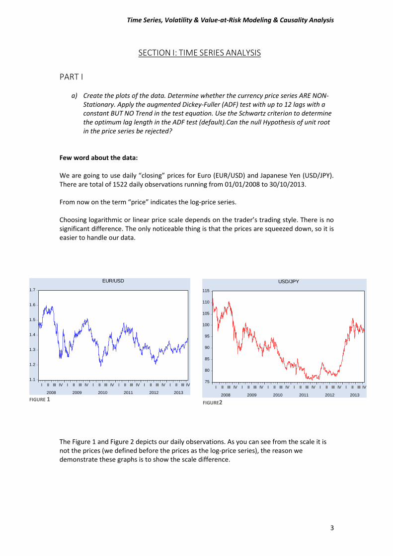
Few word about the data: We are going to use daily “closing” prices for Euro (EUR/USD) and Japanese Yen (USD/JPY). There are total of 1522 daily observations running from 01/01/2008 to 30/10/2013. From now on the term “price” indicates the log-price series. Choosing logarithmic or linear price scale depends on the trader’s trading style. There is no significant difference. The only noticeable thing is that the prices are squeezed down, so it is easier to handle our data.
The Figure 1 and Figure 2 depicts our daily observations. As you can see from the scale it is not the prices (we defined before the prices as the log-price series), the reason we demonstrate these graphs is to show the scale difference.
1.1
1.2
1.3
1.4
1.5
1.6
1.7
I II III IV I II III IV I II III IV I II III IV I II III IV I II III IV
2008 2009 2010 2011 2012 2013
EUR/USD
75
80
85
90
95
100
105
110
115
I II III IV I II III IV I II III IV I II III IV I II III IV I II III IV
2008 2009 2010 2011 2012 2013
USD/JPY
FIGURE 1
FIGURE2
Time Series, Volatility & Value-at-Risk Modeling & Causality Analysis
4
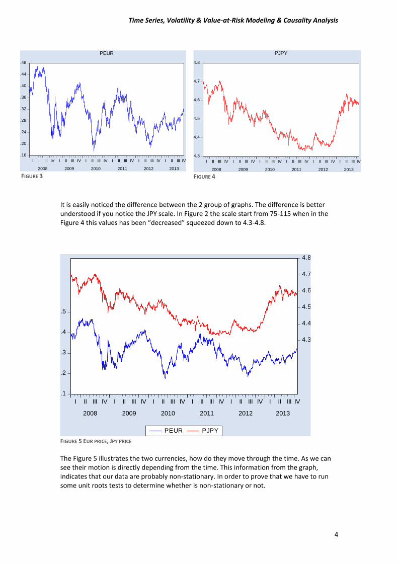
It is easily noticed the difference between the 2 group of graphs. The difference is better understood if you notice the JPY scale. In Figure 2 the scale start from 75-115 when in the Figure 4 this values has been “decreased” squeezed down to 4.3-4.8.
FIGURE 5 EUR PRICE, JPY PRICE
The Figure 5 illustrates the two currencies, how do they move through the time. As we can see their motion is directly depending from the time. This information from the graph, indicates that our data are probably non-stationary. In order to prove that we have to run some unit roots tests to determine whether is non-stationary or not.
.1
.2
.3
.4
.5
4.3
4.4
4.5
4.6
4.7
4.8
I II III IV I II III IV I II III IV I II III IV I II III IV I II III IV
2008 2009 2010 2011 2012 2013
PEUR PJPY
.16
.20
.24
.28
.32
.36
.40
.44
.48
I II III IV I II III IV I II III IV I II III IV I II III IV I II III IV
2008 2009 2010 2011 2012 2013
PEUR
4.3
4.4
4.5
4.6
4.7
4.8
I II III IV I II III IV I II III IV I II III IV I II III IV I II III IV
2008 2009 2010 2011 2012 2013
PJPY
FIGURE 3 FIGURE 4
Time Series, Volatility & Value-at-Risk Modeling & Causality Analysis
5
It would be a great mistake if we analyze our data in this primal stage, without having computed the Unit Root tests. To explain why, if you generate a regression with non-stationary time series data you may have a big R-square, but the whole regression is completely useless and has not any economic importance. So the next step is to apply the Augmented Dickey-Fuller test to our data in order to determine if our data are stationary or not-stationary. Augmented Dickey Fuller (ADF) test. Dickey-Fuller have proposed three specifications for the unit root test. In our project we are going to use the one with a constant but no trend. 𝛥𝑌𝑡 = 𝛾𝑌𝑡−𝑖 + 𝛼 + ∑ 𝛽𝑖 𝛥𝛶𝑡−𝑖 + 휀𝑖 (1.1)
𝛥𝑌𝑡 = (𝑝 − 1)𝑌𝑡−𝑖 + 𝛼 + ∑ 𝛽𝑖 𝛥𝛶𝑡−𝑖 + 휀𝑖 (1.2)
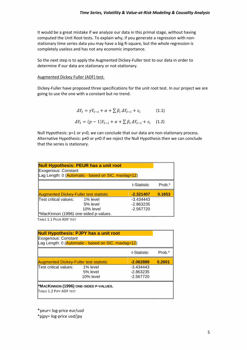
Null Hypothesis: p=1 or γ=0, we can conclude that our data are non-stationary process. Alternative Hypothesis: p≠0 or γ≠0 if we reject the Null Hypothesis then we can conclude that the series is stationary.
Null Hypothesis: PEUR has a unit root Exogenous: Constant Lag Length: 0 (Automatic - based on SIC, maxlag=12)
t-Statistic Prob.* Augmented Dickey-Fuller test statistic -2.321407 0.1653
Test critical values: 1% level -3.434443 5% level -2.863235 10% level -2.567720
*MacKinnon (1996) one-sided p-values.
TABLE 1.1 PEUR ADF TEST
*peur= log-price eur/usd *pjpy= log-price usd/jpy
Null Hypothesis: PJPY has a unit root Exogenous: Constant Lag Length: 0 (Automatic - based on SIC, maxlag=12)
t-Statistic Prob.* Augmented Dickey-Fuller test statistic -2.062889 0.2601
Test critical values: 1% level -3.434443 5% level -2.863235 10% level -2.567720 *MACKINNON (1996) ONE-SIDED P-VALUES.
TABLE 1.2 PJPY ADF TEST
Time Series, Volatility & Value-at-Risk Modeling & Causality Analysis
6
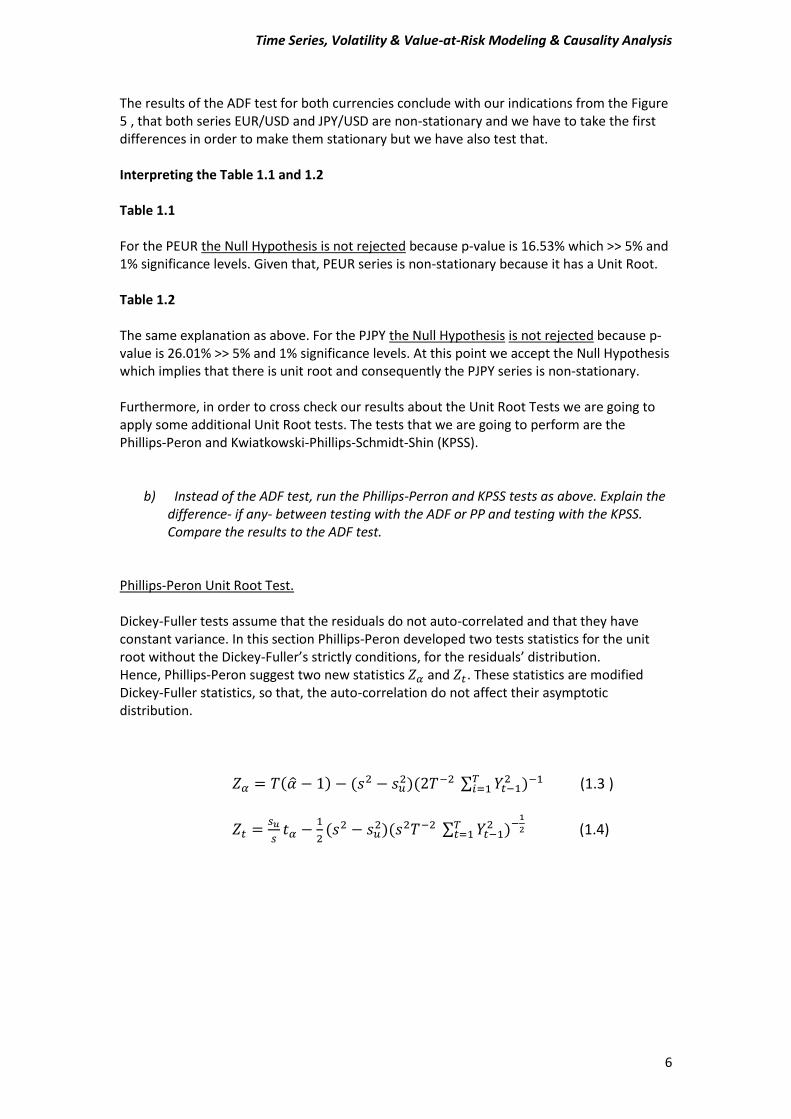
The results of the ADF test for both currencies conclude with our indications from the Figure 5 , that both series EUR/USD and JPY/USD are non-stationary and we have to take the first differences in order to make them stationary but we have also test that. Interpreting the Table 1.1 and 1.2 Table 1.1 For the PEUR the Null Hypothesis is not rejected because p-value is 16.53% which >> 5% and 1% significance levels. Given that, PEUR series is non-stationary because it has a Unit Root. Table 1.2 The same explanation as above. For the PJPY the Null Hypothesis is not rejected because p-value is 26.01% >> 5% and 1% significance levels. At this point we accept the Null Hypothesis which implies that there is unit root and consequently the PJPY series is non-stationary. Furthermore, in order to cross check our results about the Unit Root Tests we are going to apply some additional Unit Root tests. The tests that we are going to perform are the Phillips-Peron and Kwiatkowski-Phillips-Schmidt-Shin (KPSS).
b) Instead of the ADF test, run the Phillips-Perron and KPSS tests as above. Explain the difference- if any- between testing with the ADF or PP and testing with the KPSS. Compare the results to the ADF test.
Phillips-Peron Unit Root Test. Dickey-Fuller tests assume that the residuals do not auto-correlated and that they have constant variance. In this section Phillips-Peron developed two tests statistics for the unit root without the Dickey-Fuller’s strictly conditions, for the residuals’ distribution. Hence, Phillips-Peron suggest two new statistics 𝛧𝛼 and 𝛧𝑡. These statistics are modified Dickey-Fuller statistics, so that, the auto-correlation do not affect their asymptotic distribution.
𝑍𝛼 = 𝛵(�̂� − 1) − (𝑠2 − 𝑠𝑢2)(2𝑇−2 ∑ 𝑌𝑡−1
2 )−1𝑇𝑖=1 (1.3 )
𝑍𝑡 =𝑠𝑢
𝑠𝑡𝛼 −
1
2(𝑠2 − 𝑠𝑢
2)(𝑠2𝑇−2 ∑ 𝑌𝑡−12 )−
1
2𝑇𝑡=1 (1.4)
Time Series, Volatility & Value-at-Risk Modeling & Causality Analysis
7
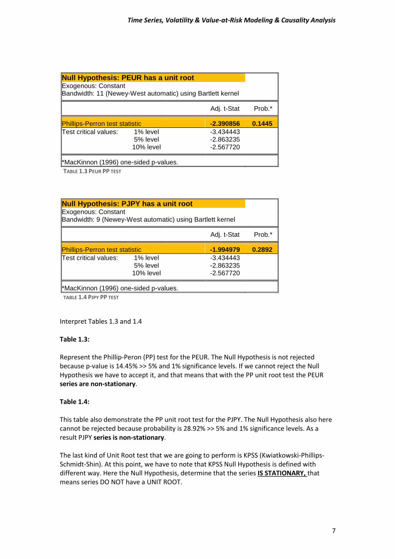
Null Hypothesis: PEUR has a unit root Exogenous: Constant Bandwidth: 11 (Newey-West automatic) using Bartlett kernel
Adj. t-Stat Prob.* Phillips-Perron test statistic -2.390856 0.1445
Test critical values: 1% level -3.434443 5% level -2.863235 10% level -2.567720 *MacKinnon (1996) one-sided p-values.
TABLE 1.3 PEUR PP TEST
Null Hypothesis: PJPY has a unit root Exogenous: Constant Bandwidth: 9 (Newey-West automatic) using Bartlett kernel
Adj. t-Stat Prob.* Phillips-Perron test statistic -1.994979 0.2892
Test critical values: 1% level -3.434443 5% level -2.863235 10% level -2.567720 *MacKinnon (1996) one-sided p-values.
TABLE 1.4 PJPY PP TEST
Interpret Tables 1.3 and 1.4 Table 1.3: Represent the Phillip-Peron (PP) test for the PEUR. The Null Hypothesis is not rejected because p-value is 14.45% >> 5% and 1% significance levels. If we cannot reject the Null Hypothesis we have to accept it, and that means that with the PP unit root test the PEUR series are non-stationary. Table 1.4: This table also demonstrate the PP unit root test for the PJPY. The Null Hypothesis also here cannot be rejected because probability is 28.92% >> 5% and 1% significance levels. As a result PJPY series is non-stationary. The last kind of Unit Root test that we are going to perform is KPSS (Kwiatkowski-Phillips-Schmidt-Shin). At this point, we have to note that KPSS Null Hypothesis is defined with different way. Here the Null Hypothesis, determine that the series IS STATIONARY, that means series DO NOT have a UNIT ROOT.
Time Series, Volatility & Value-at-Risk Modeling & Causality Analysis
8
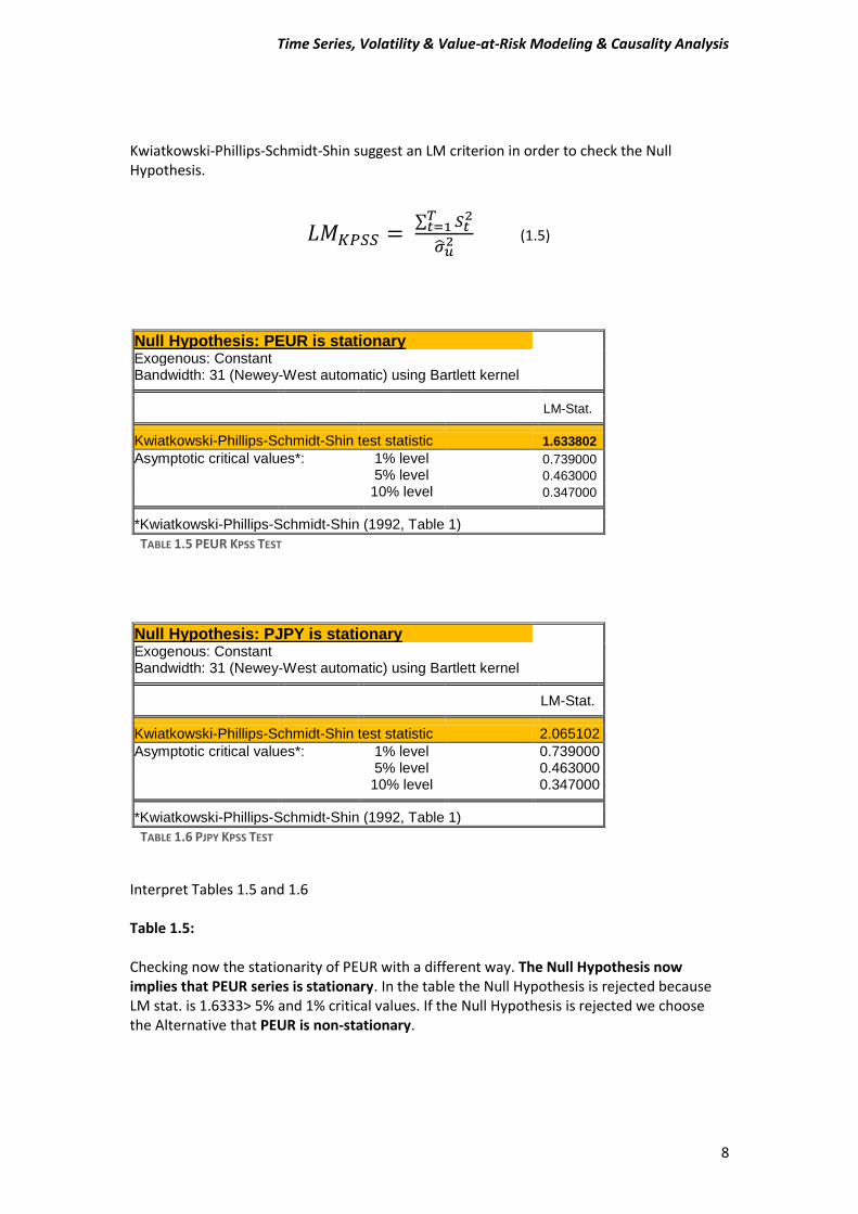
Kwiatkowski-Phillips-Schmidt-Shin suggest an LM criterion in order to check the Null Hypothesis.
𝐿𝑀𝐾𝑃𝑆𝑆 = ∑ 𝑆𝑡
2𝛵𝑡=1
�̂�𝑢2 (1.5)
Null Hypothesis: PEUR is stationary
Exogenous: Constant
Bandwidth: 31 (Newey-West automatic) using Bartlett kernel LM-Stat.
Kwiatkowski-Phillips-Schmidt-Shin test statistic 1.633802
Asymptotic critical values*: 1% level 0.739000
5% level 0.463000
10% level 0.347000
*Kwiatkowski-Phillips-Schmidt-Shin (1992, Table 1)
TABLE 1.5 PEUR KPSS TEST
Null Hypothesis: PJPY is stationary Exogenous: Constant Bandwidth: 31 (Newey-West automatic) using Bartlett kernel
LM-Stat. Kwiatkowski-Phillips-Schmidt-Shin test statistic 2.065102
Asymptotic critical values*: 1% level 0.739000 5% level 0.463000 10% level 0.347000 *Kwiatkowski-Phillips-Schmidt-Shin (1992, Table 1)
TABLE 1.6 PJPY KPSS TEST
Interpret Tables 1.5 and 1.6 Table 1.5: Checking now the stationarity of PEUR with a different way. The Null Hypothesis now implies that PEUR series is stationary. In the table the Null Hypothesis is rejected because LM stat. is 1.6333> 5% and 1% critical values. If the Null Hypothesis is rejected we choose the Alternative that PEUR is non-stationary.
Time Series, Volatility & Value-at-Risk Modeling & Causality Analysis
9
Table 1.6: Same with the previous explanation. The LM stat. for the PJPY series is 2.065102> that 5% and 1% critical values. That means, Null Hypothesis is rejected, that the series is stationary and we accept the Alternative. In other words PJPY is also non-stationary. At this stage we have completed all the diagnostic tests for the existence of Unit Root. In order to overcome the stationarity obstacle, we will take the first differences and we will check again for the existence of unit root. If at the first differences there is not unit root then we can go further to our analysis, otherwise we will have to take the second differences and then to perform again the test for unit root and so on.
Time Series, Volatility & Value-at-Risk Modeling & Causality Analysis
10
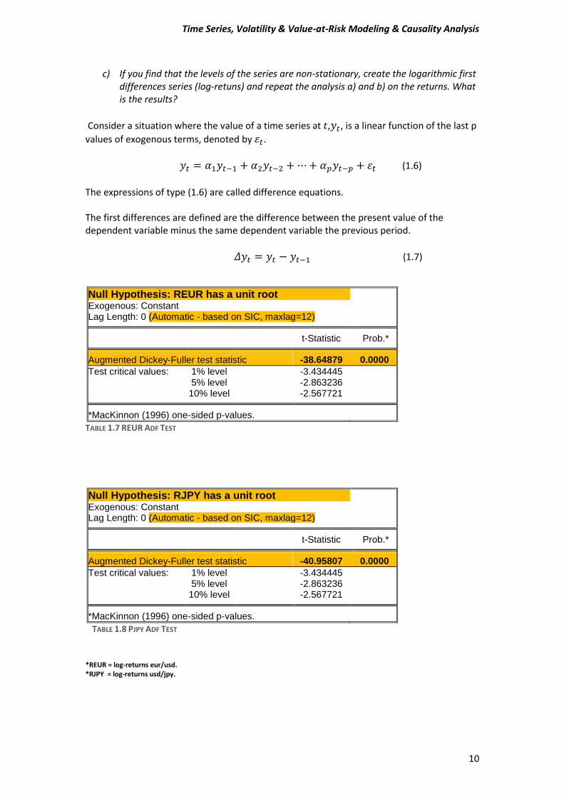
c) If you find that the levels of the series are non-stationary, create the logarithmic first differences series (log-retuns) and repeat the analysis a) and b) on the returns. What is the results?
Consider a situation where the value of a time series at 𝑡,𝑦𝑡, is a linear function of the last p
values of exogenous terms, denoted by 휀𝑡.
𝑦𝑡 = 𝛼1𝑦𝑡−1 + 𝛼2𝑦𝑡−2 + ⋯ + 𝛼𝑝𝑦𝑡−𝑝 + 휀𝑡 (1.6)
The expressions of type (1.6) are called difference equations. The first differences are defined are the difference between the present value of the dependent variable minus the same dependent variable the previous period.
𝛥𝑦𝑡 = 𝑦𝑡 − 𝑦𝑡−1 (1.7)
Null Hypothesis: REUR has a unit root Exogenous: Constant Lag Length: 0 (Automatic - based on SIC, maxlag=12)
t-Statistic Prob.* Augmented Dickey-Fuller test statistic -38.64879 0.0000
Test critical values: 1% level -3.434445 5% level -2.863236 10% level -2.567721 *MacKinnon (1996) one-sided p-values.
TABLE 1.7 REUR ADF TEST
Null Hypothesis: RJPY has a unit root Exogenous: Constant Lag Length: 0 (Automatic - based on SIC, maxlag=12)
t-Statistic Prob.* Augmented Dickey-Fuller test statistic -40.95807 0.0000
Test critical values: 1% level -3.434445 5% level -2.863236 10% level -2.567721 *MacKinnon (1996) one-sided p-values.
TABLE 1.8 PJPY ADF TEST
*REUR = log-returns eur/usd. *RJPY = log-returns usd/jpy.
Time Series, Volatility & Value-at-Risk Modeling & Causality Analysis
11
Interpret Tables 1.7 and 1.8 Table 1.7: After taking the first differences, the Null Hypothesis of the ADF test is rejected, because probability is 0.000. We accept the Alternative, so REUR series is no longer non-stationary because it has not unit root. Table 1.8: Same results also for the RJPY series. The Null Hypothesis is rejected, because probability is 0.000, given that the RJPY series is stationary.
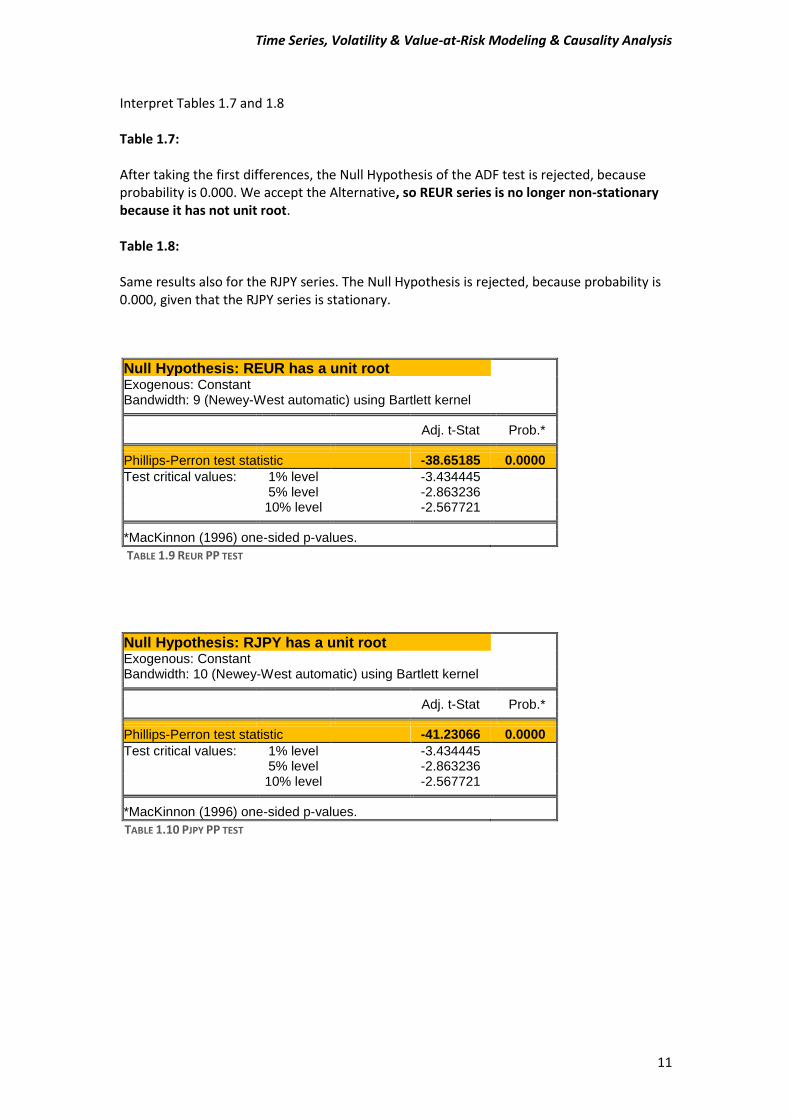
Null Hypothesis: REUR has a unit root Exogenous: Constant Bandwidth: 9 (Newey-West automatic) using Bartlett kernel
Adj. t-Stat Prob.* Phillips-Perron test statistic -38.65185 0.0000
Test critical values: 1% level -3.434445 5% level -2.863236 10% level -2.567721 *MacKinnon (1996) one-sided p-values.
TABLE 1.9 REUR PP TEST
Null Hypothesis: RJPY has a unit root Exogenous: Constant Bandwidth: 10 (Newey-West automatic) using Bartlett kernel
Adj. t-Stat Prob.* Phillips-Perron test statistic -41.23066 0.0000
Test critical values: 1% level -3.434445 5% level -2.863236 10% level -2.567721 *MacKinnon (1996) one-sided p-values.
TABLE 1.10 PJPY PP TEST
Time Series, Volatility & Value-at-Risk Modeling & Causality Analysis
12
Interpreting Tables 1.9 and 1.10 Table 1.9: Philips-Peron proves that the REUR series is stationary, because with probability 0.000 we can reject the Null Hypothesis and to accept the Alternative Hypothesis. Table 1.10 The same output has for the RJPY the Philips-Peron test. The Null Hypothesis of unit root is rejected because the probability is 0.000 and our series is stationary.
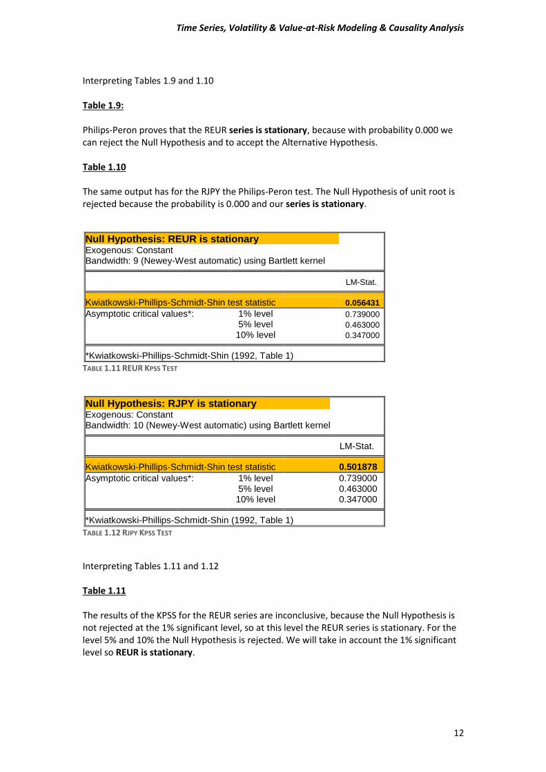
Null Hypothesis: REUR is stationary
Exogenous: Constant
Bandwidth: 9 (Newey-West automatic) using Bartlett kernel LM-Stat.
Kwiatkowski-Phillips-Schmidt-Shin test statistic 0.056431
Asymptotic critical values*: 1% level 0.739000
5% level 0.463000
10% level 0.347000
*Kwiatkowski-Phillips-Schmidt-Shin (1992, Table 1)
TABLE 1.11 REUR KPSS TEST
Null Hypothesis: RJPY is stationary Exogenous: Constant Bandwidth: 10 (Newey-West automatic) using Bartlett kernel
LM-Stat. Kwiatkowski-Phillips-Schmidt-Shin test statistic 0.501878
Asymptotic critical values*: 1% level 0.739000 5% level 0.463000 10% level 0.347000 *Kwiatkowski-Phillips-Schmidt-Shin (1992, Table 1)
TABLE 1.12 RJPY KPSS TEST
Interpreting Tables 1.11 and 1.12 Table 1.11 The results of the KPSS for the REUR series are inconclusive, because the Null Hypothesis is not rejected at the 1% significant level, so at this level the REUR series is stationary. For the level 5% and 10% the Null Hypothesis is rejected. We will take in account the 1% significant level so REUR is stationary.
Time Series, Volatility & Value-at-Risk Modeling & Causality Analysis
13
Table 1.12 The KPSS’s test result are the same for the RJPY series. The Null Hypothesis of stationarity is not rejected only at 1% significance level when at 5% and 10% the Null Hypothesis is rejected.
d) If the levels of the series are non-stationary, test for cointergration between them using the Engle-granger approach on a regression estimation. Would you have expected the series cointergrate? Why or why not? What would this tell you about their long-term relationship?
e) Perform diagnostic analysis on the residuals of the regression equation. Firstly plot
the residuals. Employ the ADF test on the residuals series assuming that up to 12 lags are permitted, and that a constant but not a trend is included in the regression on the level prices. What is the result? Is the Null Hypothesis of unit root rejected? Are the two series cointergrated or not?
We have the variables Y, 𝑋1 𝑋2, … , 𝑋𝑘 and we assume that there is long-turn relationship between them.
𝑌𝑡 = 𝑎𝑜 + 𝑎1𝑋1𝑡 + 𝑎2𝑋2𝑡 + ⋯ + 𝑎𝑘𝑋𝑘𝑡 + 𝑢𝑡 (1.8) We make an assumption that all variables are integrated I(1), so they will be cointergrated if their linear combination:
𝑢𝑡 = 𝑌𝑡 − 𝑎0 − 𝑎1𝑋1𝑡 − 𝑎2𝑋2𝑡 − ⋯ − 𝑎𝑘𝑋𝑘𝑡 (1.9)
Is integrated I(0), meaning that 𝑢𝑡 is a stationary series. The (1.8) equation that we have wrote before can be estimated with the OLS method and it is referred as cointergrating regression or static regression. The test for cointegration existence is relying on the residuals behavior, which have been produce from the OLS method. So if the residuals:
�̂�𝑡 = 𝑌𝑡 − �̂�0 − �̂�1𝑋1𝑡 − �̂�2𝑋2𝑡 − ⋯ − �̂�𝑘𝑋𝑘𝑡 (1.10) is a stationary series that means there is a long-run relationship between the variables. The next task for this project is to run a regression model with the levels of the series. We will run the following regressions 1) PEUR = C (1) + C (2)*PJPY 2) PJPY = C (1) + C (2)*PEUR From the previous diagnostic tests we found that the PEUR (EUR/USD log-prices) and the PJPY (JPY/USD) are non-stationary, which simple means that we cannot run a regression model, but if we do it we will be a spurious regression with no economic importance. BUT, if their residuals are I (0) (stationary), that means the variables of the models (1),(2) are cointergrated or they have long run relationship or equilibrium relationship between them.
Time Series, Volatility & Value-at-Risk Modeling & Causality Analysis
14
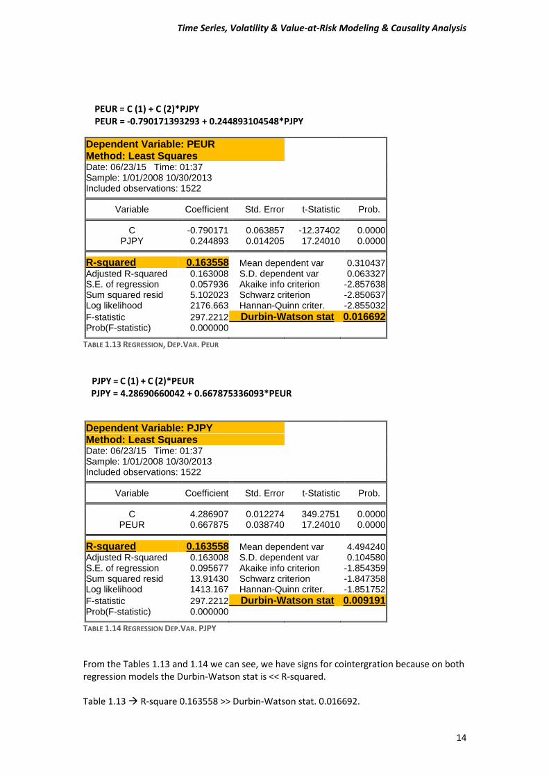
PEUR = C (1) + C (2)*PJPY PEUR = -0.790171393293 + 0.244893104548*PJPY
Dependent Variable: PEUR
Method: Least Squares Date: 06/23/15 Time: 01:37 Sample: 1/01/2008 10/30/2013 Included observations: 1522
Variable Coefficient Std. Error t-Statistic Prob. C -0.790171 0.063857 -12.37402 0.0000
PJPY 0.244893 0.014205 17.24010 0.0000 R-squared 0.163558 Mean dependent var 0.310437
Adjusted R-squared 0.163008 S.D. dependent var 0.063327 S.E. of regression 0.057936 Akaike info criterion -2.857638 Sum squared resid 5.102023 Schwarz criterion -2.850637 Log likelihood 2176.663 Hannan-Quinn criter. -2.855032
F-statistic 297.2212 Durbin-Watson stat 0.016692 Prob(F-statistic) 0.000000
TABLE 1.13 REGRESSION, DEP.VAR. PEUR PJPY = C (1) + C (2)*PEUR
PJPY = 4.28690660042 + 0.667875336093*PEUR
Dependent Variable: PJPY
Method: Least Squares Date: 06/23/15 Time: 01:37 Sample: 1/01/2008 10/30/2013 Included observations: 1522
Variable Coefficient Std. Error t-Statistic Prob. C 4.286907 0.012274 349.2751 0.0000
PEUR 0.667875 0.038740 17.24010 0.0000 R-squared 0.163558 Mean dependent var 4.494240
Adjusted R-squared 0.163008 S.D. dependent var 0.104580 S.E. of regression 0.095677 Akaike info criterion -1.854359 Sum squared resid 13.91430 Schwarz criterion -1.847358 Log likelihood 1413.167 Hannan-Quinn criter. -1.851752
F-statistic 297.2212 Durbin-Watson stat 0.009191 Prob(F-statistic) 0.000000
TABLE 1.14 REGRESSION DEP.VAR. PJPY
From the Tables 1.13 and 1.14 we can see, we have signs for cointergration because on both regression models the Durbin-Watson stat is << R-squared. Table 1.13 R-square 0.163558 >> Durbin-Watson stat. 0.016692.
Time Series, Volatility & Value-at-Risk Modeling & Causality Analysis
15
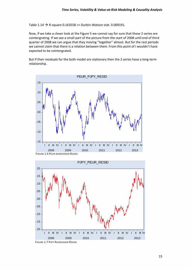
Table 1.14 R-square 0.163558 >> Durbin-Watson stat. 0.009191. Now, if we take a closer look at the Figure 5 we cannot say for sure that these 2 series are cointergrating. If we see a small part of the picture from the start of 2008 until end of third quarter of 2008 we can argue that they moving “together” almost. But for the rest periods we cannot claim that there is a relation between them. From this point of I wouldn’t have expected to be cointergrated. But if their residuals for the both model are stationary then the 2 series have a long-term relationship.
FIGURE 1.6 PEUR REGRESSION RESIDS
-.15
-.10
-.05
.00
.05
.10
.15
I II III IV I II III IV I II III IV I II III IV I II III IV I II III IV
2008 2009 2010 2011 2012 2013
PEUR_PJPY_RESID
-.20
-.15
-.10
-.05
.00
.05
.10
.15
.20
I II III IV I II III IV I II III IV I II III IV I II III IV I II III IV
2008 2009 2010 2011 2012 2013
PJPY_PEUR_RESID
FIGURE 1.7 PJPY REGRESSION RESIDS
Time Series, Volatility & Value-at-Risk Modeling & Causality Analysis
16
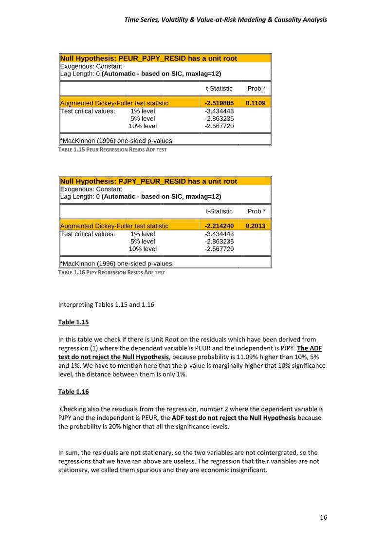
Null Hypothesis: PEUR_PJPY_RESID has a unit root Exogenous: Constant Lag Length: 0 (Automatic - based on SIC, maxlag=12)
t-Statistic Prob.* Augmented Dickey-Fuller test statistic -2.519885 0.1109
Test critical values: 1% level -3.434443 5% level -2.863235 10% level -2.567720 *MacKinnon (1996) one-sided p-values.
TABLE 1.15 PEUR REGRESSION RESIDS ADF TEST
Null Hypothesis: PJPY_PEUR_RESID has a unit root Exogenous: Constant Lag Length: 0 (Automatic - based on SIC, maxlag=12)
t-Statistic Prob.* Augmented Dickey-Fuller test statistic -2.214240 0.2013
Test critical values: 1% level -3.434443 5% level -2.863235 10% level -2.567720 *MacKinnon (1996) one-sided p-values.
TABLE 1.16 PJPY REGRESSION RESIDS ADF TEST
Interpreting Tables 1.15 and 1.16 Table 1.15 In this table we check if there is Unit Root on the residuals which have been derived from regression (1) where the dependent variable is PEUR and the independent is PJPY. The ADF test do not reject the Null Hypothesis, because probability is 11.09% higher than 10%, 5% and 1%. We have to mention here that the p-value is marginally higher that 10% significance level, the distance between them is only 1%. Table 1.16 Checking also the residuals from the regression, number 2 where the dependent variable is PJPY and the independent is PEUR, the ADF test do not reject the Null Hypothesis because the probability is 20% higher that all the significance levels. In sum, the residuals are not stationary, so the two variables are not cointergrated, so the regressions that we have ran above are useless. The regression that their variables are not stationary, we called them spurious and they are economic insignificant.
Time Series, Volatility & Value-at-Risk Modeling & Causality Analysis
17
f) Based on the results of the previous question e), a pure first difference equation model or an error correction model (ECM) is appropriate in order to capture the long-run relationship between the series as well as the short-run relationship? Then, estimate the ECM or the pure first difference equation model based on the results of question e) and describe the cointergration relationship based on the Engle-Granger approach, or the short-run relationship between the variables.
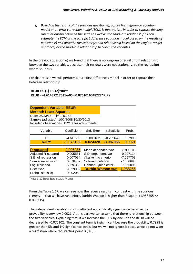
In the previous question e) we found that there is no long-run or equilibrium relationship between the two variables, because their residuals were not stationary, so the regression where spurious. For that reason we will perform a pure first differences model in order to capture their between relationship. REUR = C (1) + C (2)*RJPY REUR = -4.61437217621e-05 - 0.0751016048227*RJPY
Dependent Variable: REUR
Method: Least Squares Date: 06/23/15 Time: 01:48 Sample (adjusted): 1/02/2008 10/30/2013 Included observations: 1521 after adjustments
Variable Coefficient Std. Error t-Statistic Prob. C -4.61E-05 0.000182 -0.253649 0.7998
RJPY -0.075102 0.024328 -3.087065 0.0021 R-squared 0.006235 Mean dependent var -3.99E-05
Adjusted R-squared 0.005581 S.D. dependent var 0.007114 S.E. of regression 0.007094 Akaike info criterion -7.057703 Sum squared resid 0.076452 Schwarz criterion -7.050698 Log likelihood 5369.383 Hannan-Quinn criter. -7.055095
F-statistic 9.529969 Durbin-Watson stat 1.988255 Prob(F-statistic) 0.002058
TABLE 1.17 REUR REGRESSION MODEL
From the Table 1.17, we can see now the reverse results in contrast with the spurious regression that we have ran before. Durbin-Watson is higher than R-square (1.988255 >> 0.006235)
The independent variable’s RJPY coefficient is statistically significance because the provability is very low 0.0021. At this part we can assume that there is relationship between the two variables. Explaining that, if we increase the RJPY by one unit the REUR will be decreased by -0.075102. The constant term is insignificant because the probability 0.7998 is greater than 5% and 1% significance levels, but we will not ignore it because we do not want a regression where the starting point is (0,0).
Time Series, Volatility & Value-at-Risk Modeling & Causality Analysis
18
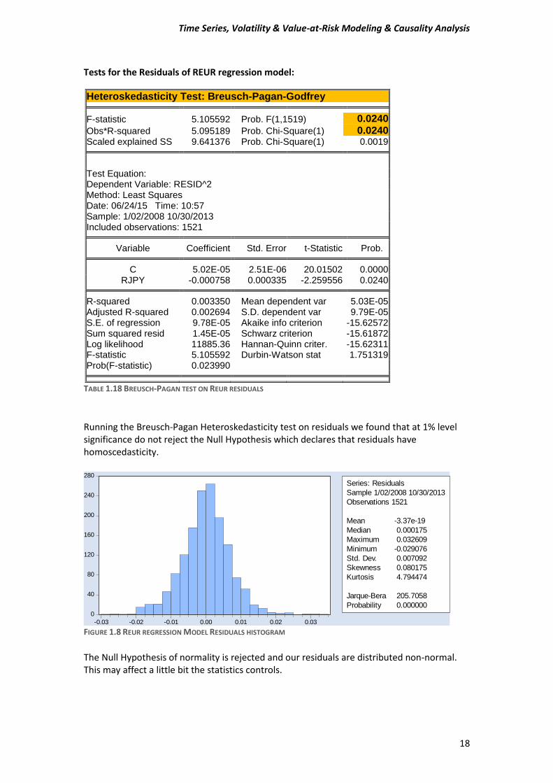
Tests for the Residuals of REUR regression model:
Heteroskedasticity Test: Breusch-Pagan-Godfrey
F-statistic 5.105592 Prob. F(1,1519) 0.0240
Obs*R-squared 5.095189 Prob. Chi-Square(1) 0.0240 Scaled explained SS 9.641376 Prob. Chi-Square(1) 0.0019
Test Equation: Dependent Variable: RESID^2 Method: Least Squares Date: 06/24/15 Time: 10:57 Sample: 1/02/2008 10/30/2013 Included observations: 1521
Variable Coefficient Std. Error t-Statistic Prob. C 5.02E-05 2.51E-06 20.01502 0.0000
RJPY -0.000758 0.000335 -2.259556 0.0240 R-squared 0.003350 Mean dependent var 5.03E-05
Adjusted R-squared 0.002694 S.D. dependent var 9.79E-05 S.E. of regression 9.78E-05 Akaike info criterion -15.62572 Sum squared resid 1.45E-05 Schwarz criterion -15.61872 Log likelihood 11885.36 Hannan-Quinn criter. -15.62311 F-statistic 5.105592 Durbin-Watson stat 1.751319 Prob(F-statistic) 0.023990
TABLE 1.18 BREUSCH-PAGAN TEST ON REUR RESIDUALS
Running the Breusch-Pagan Heteroskedasticity test on residuals we found that at 1% level significance do not reject the Null Hypothesis which declares that residuals have homoscedasticity.
FIGURE 1.8 REUR REGRESSION MODEL RESIDUALS HISTOGRAM
The Null Hypothesis of normality is rejected and our residuals are distributed non-normal. This may affect a little bit the statistics controls.
0
40
80
120
160
200
240
280
-0.03 -0.02 -0.01 0.00 0.01 0.02 0.03
Series: Residuals
Sample 1/02/2008 10/30/2013
Observations 1521
Mean -3.37e-19
Median 0.000175
Maximum 0.032609
Minimum -0.029076
Std. Dev. 0.007092
Skewness 0.080175
Kurtosis 4.794474
Jarque-Bera 205.7058
Probability 0.000000
Time Series, Volatility & Value-at-Risk Modeling & Causality Analysis
19
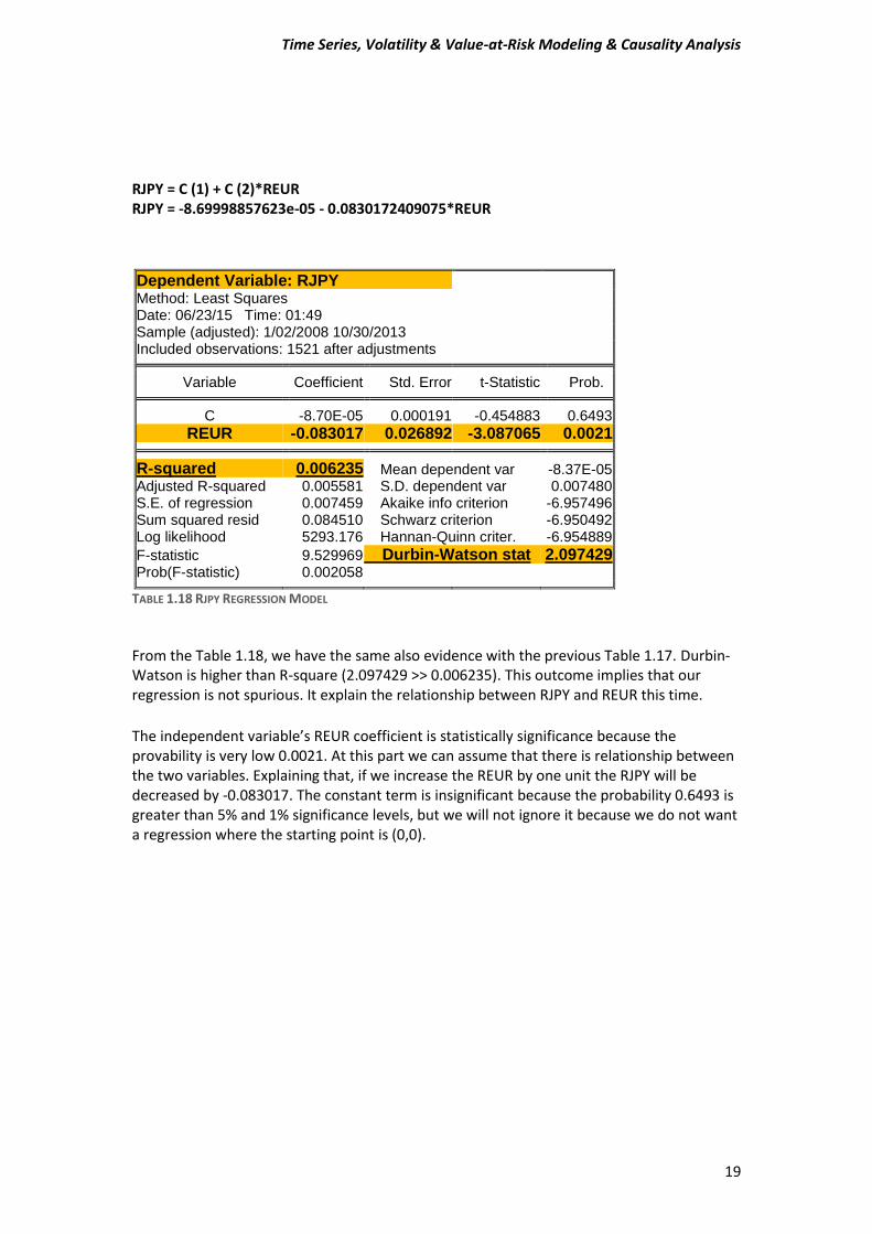
RJPY = C (1) + C (2)*REUR RJPY = -8.69998857623e-05 - 0.0830172409075*REUR
Dependent Variable: RJPY Method: Least Squares Date: 06/23/15 Time: 01:49 Sample (adjusted): 1/02/2008 10/30/2013 Included observations: 1521 after adjustments
Variable Coefficient Std. Error t-Statistic Prob. C -8.70E-05 0.000191 -0.454883 0.6493
REUR -0.083017 0.026892 -3.087065 0.0021 R-squared 0.006235 Mean dependent var -8.37E-05
Adjusted R-squared 0.005581 S.D. dependent var 0.007480 S.E. of regression 0.007459 Akaike info criterion -6.957496 Sum squared resid 0.084510 Schwarz criterion -6.950492 Log likelihood 5293.176 Hannan-Quinn criter. -6.954889
F-statistic 9.529969 Durbin-Watson stat 2.097429 Prob(F-statistic) 0.002058
TABLE 1.18 RJPY REGRESSION MODEL
From the Table 1.18, we have the same also evidence with the previous Table 1.17. Durbin-Watson is higher than R-square (2.097429 >> 0.006235). This outcome implies that our regression is not spurious. It explain the relationship between RJPY and REUR this time.
The independent variable’s REUR coefficient is statistically significance because the provability is very low 0.0021. At this part we can assume that there is relationship between the two variables. Explaining that, if we increase the REUR by one unit the RJPY will be decreased by -0.083017. The constant term is insignificant because the probability 0.6493 is greater than 5% and 1% significance levels, but we will not ignore it because we do not want a regression where the starting point is (0,0).
Time Series, Volatility & Value-at-Risk Modeling & Causality Analysis
20
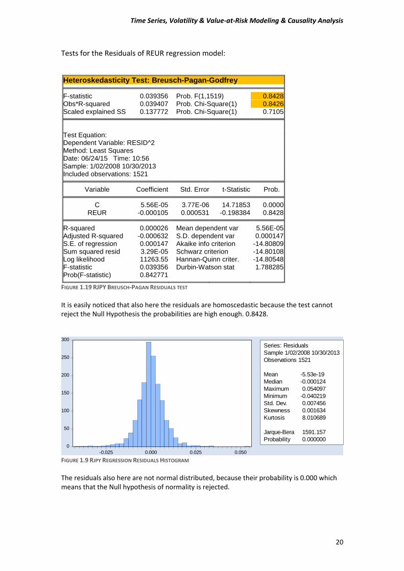
Tests for the Residuals of REUR regression model:
Heteroskedasticity Test: Breusch-Pagan-Godfrey
F-statistic 0.039356 Prob. F(1,1519) 0.8428
Obs*R-squared 0.039407 Prob. Chi-Square(1) 0.8426 Scaled explained SS 0.137772 Prob. Chi-Square(1) 0.7105
Test Equation: Dependent Variable: RESID^2 Method: Least Squares Date: 06/24/15 Time: 10:56 Sample: 1/02/2008 10/30/2013 Included observations: 1521
Variable Coefficient Std. Error t-Statistic Prob. C 5.56E-05 3.77E-06 14.71853 0.0000
REUR -0.000105 0.000531 -0.198384 0.8428 R-squared 0.000026 Mean dependent var 5.56E-05
Adjusted R-squared -0.000632 S.D. dependent var 0.000147 S.E. of regression 0.000147 Akaike info criterion -14.80809 Sum squared resid 3.29E-05 Schwarz criterion -14.80108 Log likelihood 11263.55 Hannan-Quinn criter. -14.80548 F-statistic 0.039356 Durbin-Watson stat 1.788285 Prob(F-statistic) 0.842771
FIGURE 1.19 RJPY BREUSCH-PAGAN RESIDUALS TEST
It is easily noticed that also here the residuals are homoscedastic because the test cannot reject the Null Hypothesis the probabilities are high enough. 0.8428.
FIGURE 1.9 RJPY REGRESSION RESIDUALS HISTOGRAM
The residuals also here are not normal distributed, because their probability is 0.000 which means that the Null hypothesis of normality is rejected.
0
50
100
150
200
250
300
-0.025 0.000 0.025 0.050
Series: Residuals
Sample 1/02/2008 10/30/2013
Observations 1521
Mean -5.53e-19
Median -0.000124
Maximum 0.054097
Minimum -0.040219
Std. Dev. 0.007456
Skewness 0.001634
Kurtosis 8.010689
Jarque-Bera 1591.157
Probability 0.000000
Time Series, Volatility & Value-at-Risk Modeling & Causality Analysis
21
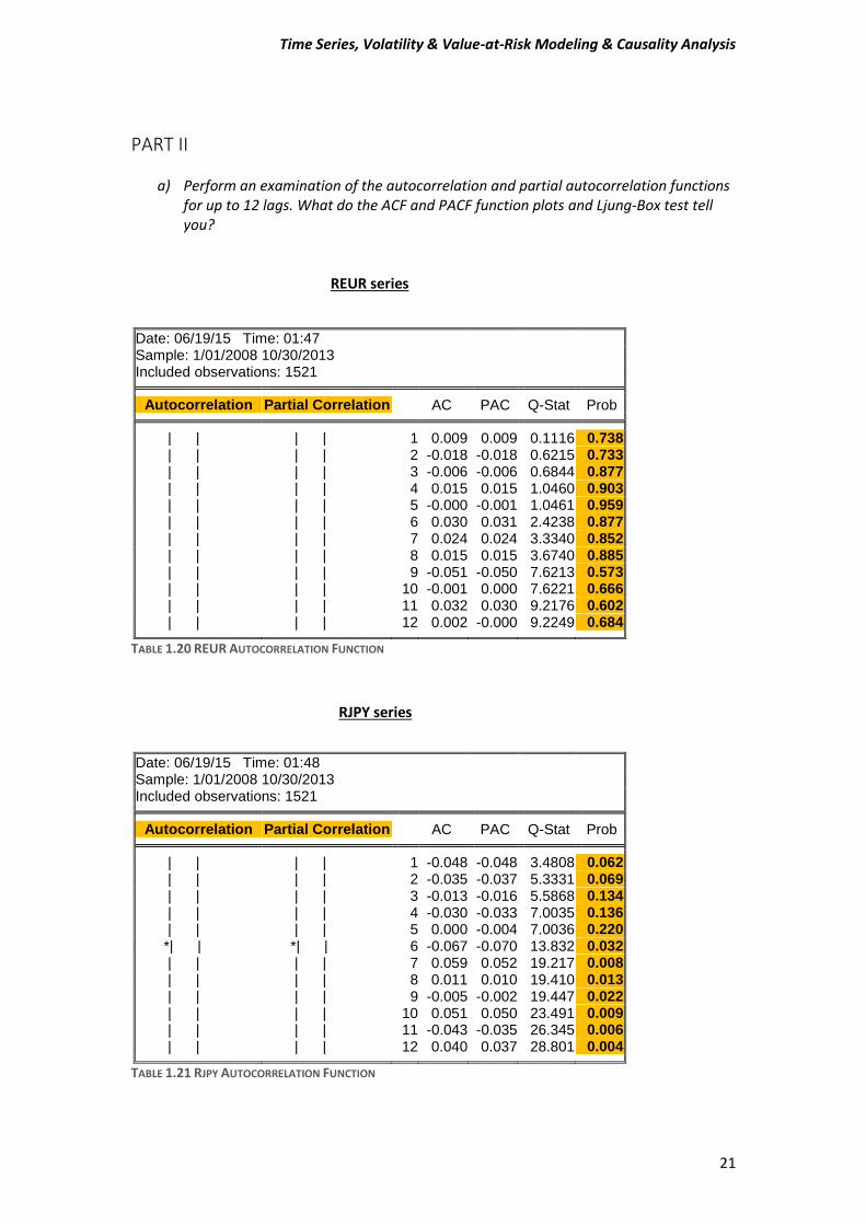
PART II
a) Perform an examination of the autocorrelation and partial autocorrelation functions for up to 12 lags. What do the ACF and PACF function plots and Ljung-Box test tell you?
REUR series
Date: 06/19/15 Time: 01:47 Sample: 1/01/2008 10/30/2013 Included observations: 1521
Autocorrelation Partial Correlation AC PAC Q-Stat Prob | | | | 1 0.009 0.009 0.1116 0.738
| | | | 2 -0.018 -0.018 0.6215 0.733 | | | | 3 -0.006 -0.006 0.6844 0.877 | | | | 4 0.015 0.015 1.0460 0.903 | | | | 5 -0.000 -0.001 1.0461 0.959 | | | | 6 0.030 0.031 2.4238 0.877 | | | | 7 0.024 0.024 3.3340 0.852 | | | | 8 0.015 0.015 3.6740 0.885 | | | | 9 -0.051 -0.050 7.6213 0.573 | | | | 10 -0.001 0.000 7.6221 0.666 | | | | 11 0.032 0.030 9.2176 0.602 | | | | 12 0.002 -0.000 9.2249 0.684
TABLE 1.20 REUR AUTOCORRELATION FUNCTION
RJPY series
Date: 06/19/15 Time: 01:48 Sample: 1/01/2008 10/30/2013 Included observations: 1521
Autocorrelation Partial Correlation AC PAC Q-Stat Prob | | | | 1 -0.048 -0.048 3.4808 0.062
| | | | 2 -0.035 -0.037 5.3331 0.069 | | | | 3 -0.013 -0.016 5.5868 0.134 | | | | 4 -0.030 -0.033 7.0035 0.136 | | | | 5 0.000 -0.004 7.0036 0.220 *| | *| | 6 -0.067 -0.070 13.832 0.032 | | | | 7 0.059 0.052 19.217 0.008 | | | | 8 0.011 0.010 19.410 0.013 | | | | 9 -0.005 -0.002 19.447 0.022 | | | | 10 0.051 0.050 23.491 0.009 | | | | 11 -0.043 -0.035 26.345 0.006 | | | | 12 0.040 0.037 28.801 0.004
TABLE 1.21 RJPY AUTOCORRELATION FUNCTION
Time Series, Volatility & Value-at-Risk Modeling & Causality Analysis
22
Interpret Table 1.20 and 1.21 Table 1.20: That we can notice here is that all coefficient of ACF and PACF are statistically insignificant. Moreover the values of the coefficients are very low almost close to zero. In other words that means that between them there is no correlation. From this point we can assume with no safety that probably REUR series is an ARMA (0, 0). Table 1.21: In contrast with the REUR series, RJPY series ACF and PACF are insignificant for the first 5 lags because their probability is higher than 10%. It is worthy to mention that the coefficient for the lag 6 are significant, and if we continue to then next lags, the probability is less than 5% which means that the series has autocorrelation. Also here the coefficients values are very low close to zero. The results here are inconclusive. The Ljung-Box test which is a modified approach, which came from the Box-Pierce test, it tests jointly the significance of autocorrelation coefficients through the residuals control.
Null Hypothesis: 𝜌1 = 𝜌2 = ⋯ = 𝜌𝑚 = 0 Ljung-Box statistic is defined as:
𝑄𝐿𝐵 = 𝑇(𝑇 + 2) ∑�̂�𝑠
2
𝑇−𝑠𝑚𝑠=1 (1.11)
Testing now with Ljung-Box statistic for the Table 1.20 the last lag number 12 the 𝑄𝐿𝐵 Do not reject the Null Hypothesis because the probability is 68.4% is high enough. That means the REUR series has no serial autocorrelation.
For the Table 1.21 the results are different. The 𝑄𝐿𝐵 reject the Null Hypothesis and accept
the alternative that the RJPY series has autocorrelation. This happens because at lag 12 the
probability of 𝑄𝐿𝐵 is less that 1% and that implies the rejection of the Null Hypothesis.
Time Series, Volatility & Value-at-Risk Modeling & Causality Analysis
23
b) Suppose that ARMA models from order (0, 0) to (2, 2) are plausible for the two currency return series. Use the information criteria AIC and SBIC for each ARMA model order from (0, 0) to (2, 2). Which models do the criteria select i.e., which model for the AIC and which for the SBIC for each return series (four models in total)? Compare the results of the information criteria to the results from ACF and PACF question a)
Representing the equations for AR (p) MA (p) and ARMA (p, q) AR (p)
𝑌𝑡 = 𝛼0 + 𝛼1𝑌𝑡−1 + 𝛼2𝑌𝑡−2 + ⋯ + 𝛼𝑝𝑌𝑡−𝑝 + 휀𝑡 (1.12)
MA (q)
𝑌𝑡 = 𝜇 + 휀𝑡 + 𝜃1휀𝑡−1 + 𝜃2휀𝑡−2 + ⋯ + 𝜃𝑝휀𝑡−𝑞 (1.13)
ARMA (p, q)
𝑌𝑡 = 𝛿 + 𝛼1𝑌𝑡−1 + 𝛼2𝑌𝑡−2 + ⋯ + 𝛼𝑝𝑌𝑡−𝑝 + 휀𝑡 + 𝜃1휀𝑡−1 + 𝜃2휀𝑡−2 +
⋯ + 𝜃𝑝휀𝑡−𝑞 (1.14)
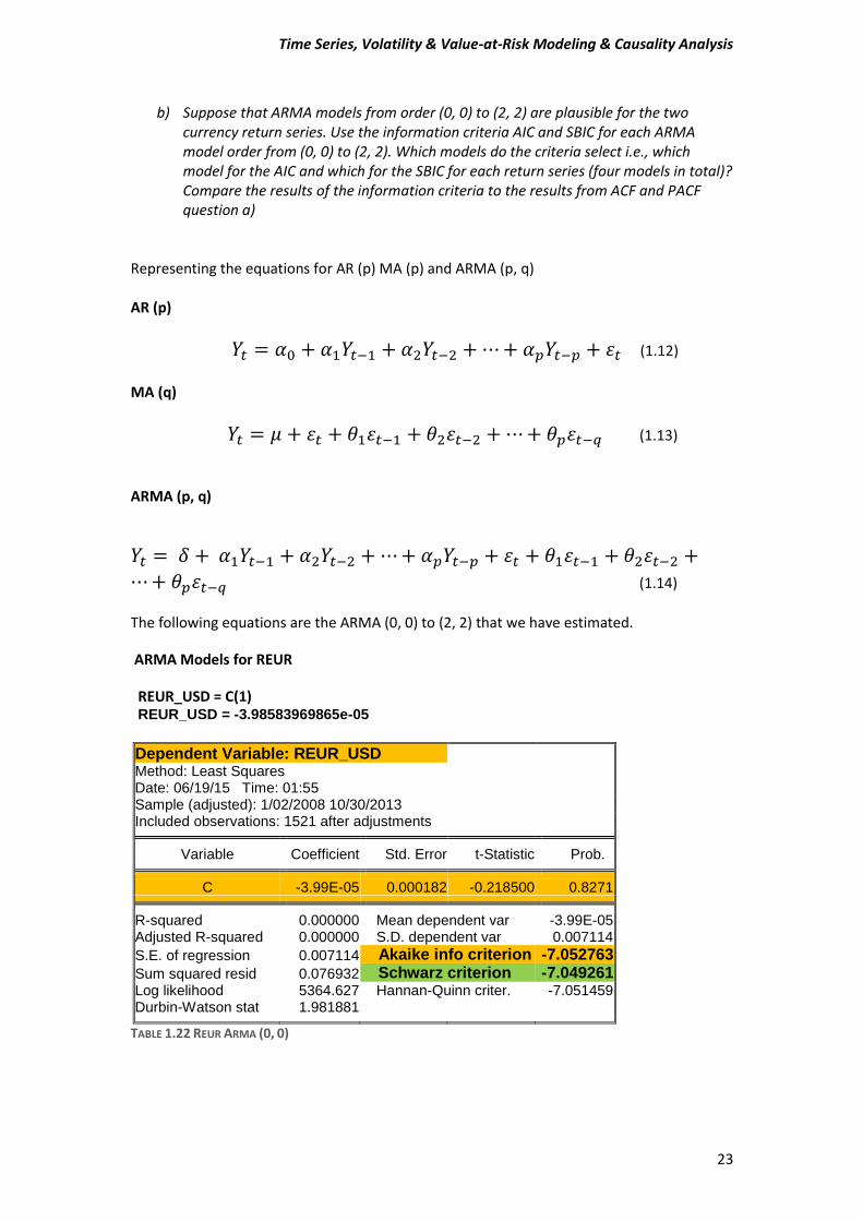
The following equations are the ARMA (0, 0) to (2, 2) that we have estimated.
ARMA Models for REUR
REUR_USD = C(1) REUR_USD = -3.98583969865e-05
Dependent Variable: REUR_USD Method: Least Squares Date: 06/19/15 Time: 01:55 Sample (adjusted): 1/02/2008 10/30/2013 Included observations: 1521 after adjustments
Variable Coefficient Std. Error t-Statistic Prob. C -3.99E-05 0.000182 -0.218500 0.8271 R-squared 0.000000 Mean dependent var -3.99E-05
Adjusted R-squared 0.000000 S.D. dependent var 0.007114
S.E. of regression 0.007114 Akaike info criterion -7.052763
Sum squared resid 0.076932 Schwarz criterion -7.049261 Log likelihood 5364.627 Hannan-Quinn criter. -7.051459 Durbin-Watson stat 1.981881
TABLE 1.22 REUR ARMA (0, 0)
Time Series, Volatility & Value-at-Risk Modeling & Causality Analysis
24
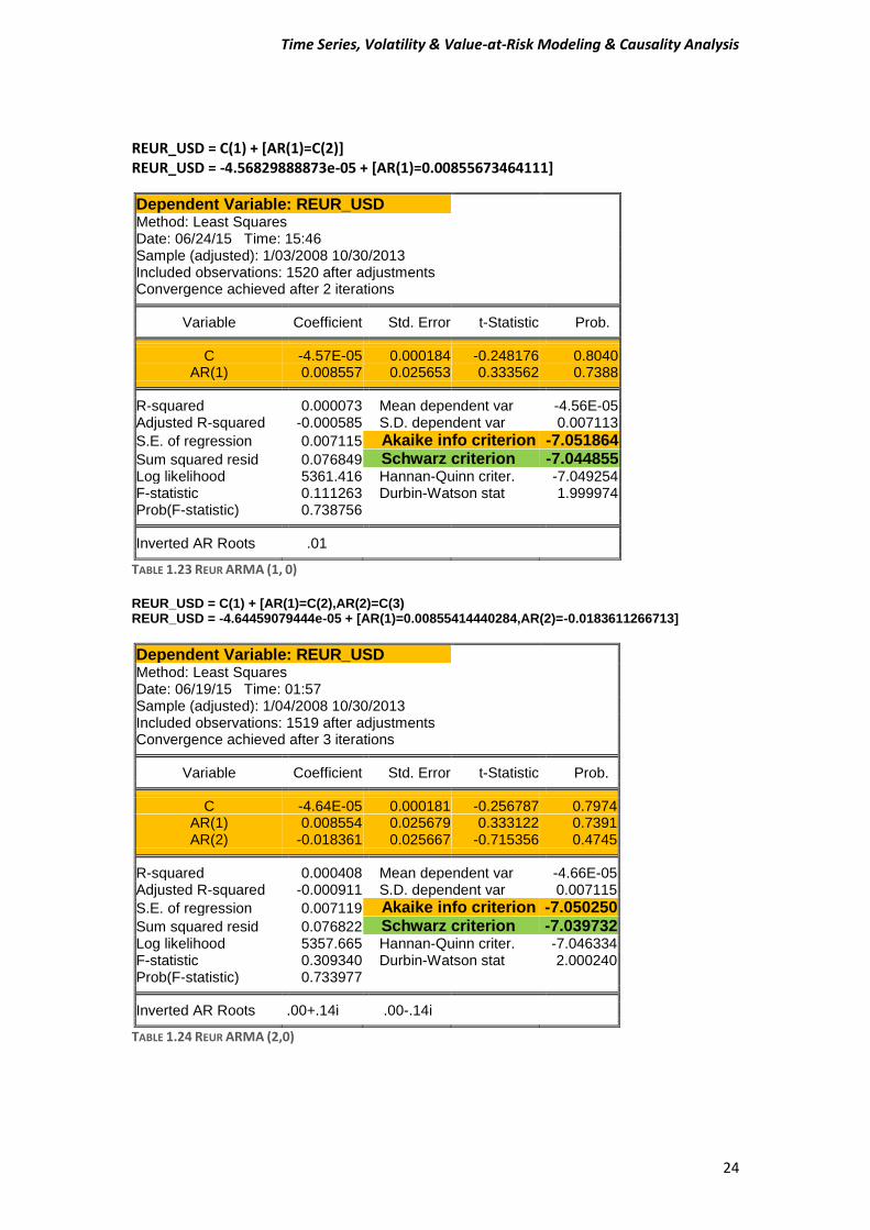
REUR_USD = C(1) + [AR(1)=C(2)] REUR_USD = -4.56829888873e-05 + [AR(1)=0.00855673464111]
Dependent Variable: REUR_USD Method: Least Squares Date: 06/24/15 Time: 15:46 Sample (adjusted): 1/03/2008 10/30/2013 Included observations: 1520 after adjustments Convergence achieved after 2 iterations
Variable Coefficient Std. Error t-Statistic Prob. C -4.57E-05 0.000184 -0.248176 0.8040
AR(1) 0.008557 0.025653 0.333562 0.7388 R-squared 0.000073 Mean dependent var -4.56E-05
Adjusted R-squared -0.000585 S.D. dependent var 0.007113
S.E. of regression 0.007115 Akaike info criterion -7.051864
Sum squared resid 0.076849 Schwarz criterion -7.044855 Log likelihood 5361.416 Hannan-Quinn criter. -7.049254 F-statistic 0.111263 Durbin-Watson stat 1.999974 Prob(F-statistic) 0.738756
Inverted AR Roots .01
TABLE 1.23 REUR ARMA (1, 0)
REUR_USD = C(1) + [AR(1)=C(2),AR(2)=C(3) REUR_USD = -4.64459079444e-05 + [AR(1)=0.00855414440284,AR(2)=-0.0183611266713]
Dependent Variable: REUR_USD Method: Least Squares Date: 06/19/15 Time: 01:57 Sample (adjusted): 1/04/2008 10/30/2013 Included observations: 1519 after adjustments Convergence achieved after 3 iterations
Variable Coefficient Std. Error t-Statistic Prob. C -4.64E-05 0.000181 -0.256787 0.7974
AR(1) 0.008554 0.025679 0.333122 0.7391 AR(2) -0.018361 0.025667 -0.715356 0.4745
R-squared 0.000408 Mean dependent var -4.66E-05
Adjusted R-squared -0.000911 S.D. dependent var 0.007115
S.E. of regression 0.007119 Akaike info criterion -7.050250
Sum squared resid 0.076822 Schwarz criterion -7.039732 Log likelihood 5357.665 Hannan-Quinn criter. -7.046334 F-statistic 0.309340 Durbin-Watson stat 2.000240 Prob(F-statistic) 0.733977
Inverted AR Roots .00+.14i .00-.14i
TABLE 1.24 REUR ARMA (2,0)
Time Series, Volatility & Value-at-Risk Modeling & Causality Analysis
25
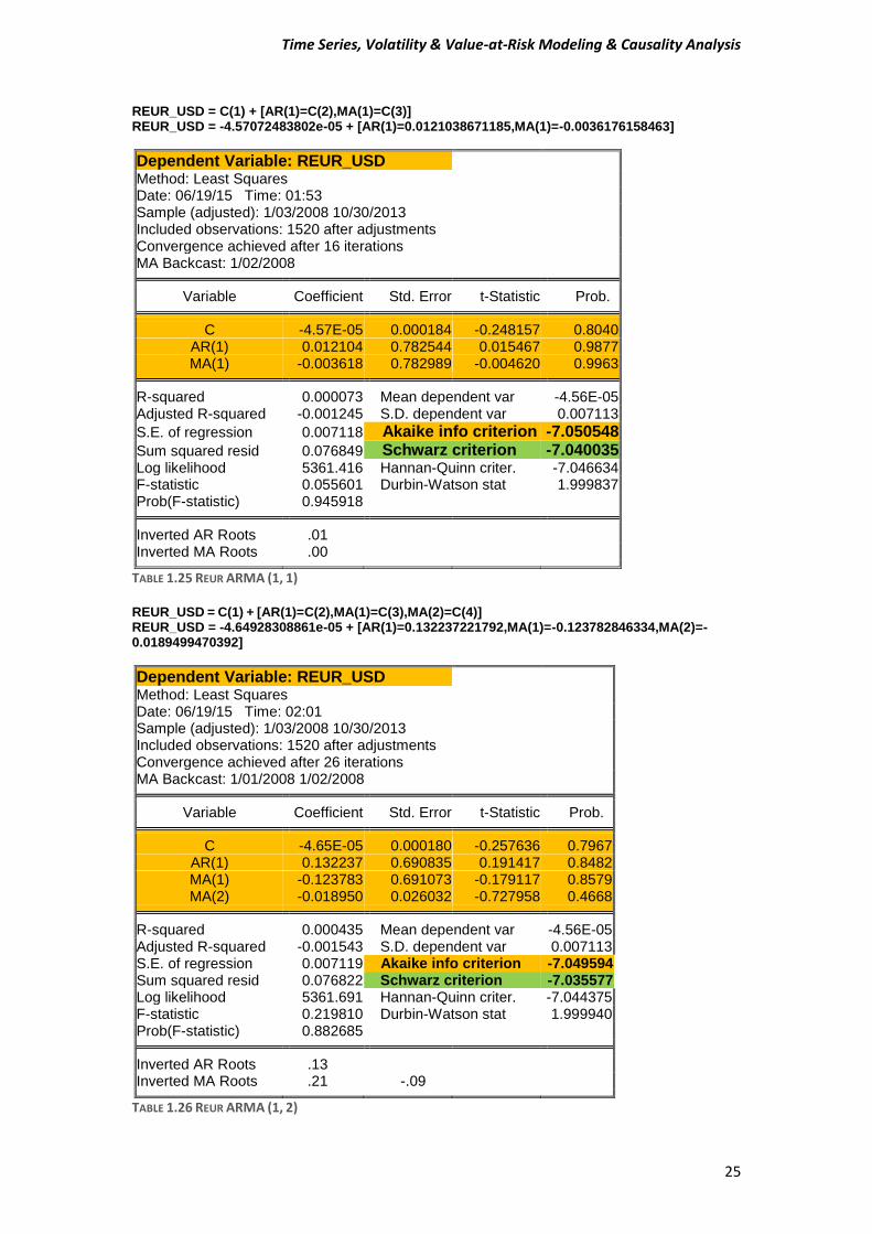
REUR_USD = C(1) + [AR(1)=C(2),MA(1)=C(3)] REUR_USD = -4.57072483802e-05 + [AR(1)=0.0121038671185,MA(1)=-0.0036176158463]
Dependent Variable: REUR_USD Method: Least Squares Date: 06/19/15 Time: 01:53 Sample (adjusted): 1/03/2008 10/30/2013 Included observations: 1520 after adjustments Convergence achieved after 16 iterations MA Backcast: 1/02/2008
Variable Coefficient Std. Error t-Statistic Prob. C -4.57E-05 0.000184 -0.248157 0.8040
AR(1) 0.012104 0.782544 0.015467 0.9877 MA(1) -0.003618 0.782989 -0.004620 0.9963
R-squared 0.000073 Mean dependent var -4.56E-05
Adjusted R-squared -0.001245 S.D. dependent var 0.007113
S.E. of regression 0.007118 Akaike info criterion -7.050548
Sum squared resid 0.076849 Schwarz criterion -7.040035 Log likelihood 5361.416 Hannan-Quinn criter. -7.046634 F-statistic 0.055601 Durbin-Watson stat 1.999837 Prob(F-statistic) 0.945918
Inverted AR Roots .01
Inverted MA Roots .00
TABLE 1.25 REUR ARMA (1, 1) REUR_USD = C(1) + [AR(1)=C(2),MA(1)=C(3),MA(2)=C(4)] REUR_USD = -4.64928308861e-05 + [AR(1)=0.132237221792,MA(1)=-0.123782846334,MA(2)=-0.0189499470392]
Dependent Variable: REUR_USD Method: Least Squares Date: 06/19/15 Time: 02:01 Sample (adjusted): 1/03/2008 10/30/2013 Included observations: 1520 after adjustments Convergence achieved after 26 iterations MA Backcast: 1/01/2008 1/02/2008
Variable Coefficient Std. Error t-Statistic Prob. C -4.65E-05 0.000180 -0.257636 0.7967
AR(1) 0.132237 0.690835 0.191417 0.8482 MA(1) -0.123783 0.691073 -0.179117 0.8579 MA(2) -0.018950 0.026032 -0.727958 0.4668
R-squared 0.000435 Mean dependent var -4.56E-05
Adjusted R-squared -0.001543 S.D. dependent var 0.007113 S.E. of regression 0.007119 Akaike info criterion -7.049594 Sum squared resid 0.076822 Schwarz criterion -7.035577 Log likelihood 5361.691 Hannan-Quinn criter. -7.044375 F-statistic 0.219810 Durbin-Watson stat 1.999940 Prob(F-statistic) 0.882685
Inverted AR Roots .13
Inverted MA Roots .21 -.09
TABLE 1.26 REUR ARMA (1, 2)
Time Series, Volatility & Value-at-Risk Modeling & Causality Analysis
26
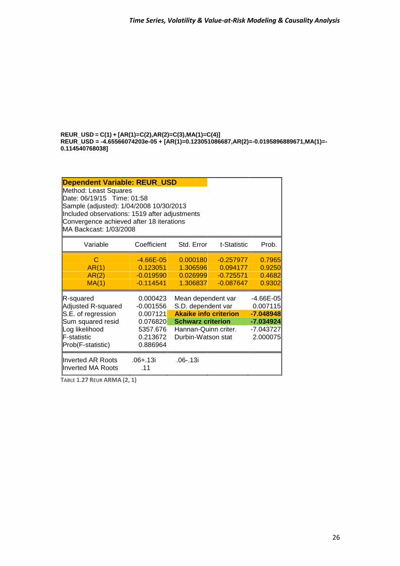
REUR_USD = C(1) + [AR(1)=C(2),AR(2)=C(3),MA(1)=C(4)] REUR_USD = -4.65566074203e-05 + [AR(1)=0.123051086687,AR(2)=-0.0195896889671,MA(1)=-0.114540768038]
Dependent Variable: REUR_USD Method: Least Squares Date: 06/19/15 Time: 01:58 Sample (adjusted): 1/04/2008 10/30/2013 Included observations: 1519 after adjustments Convergence achieved after 18 iterations MA Backcast: 1/03/2008
Variable Coefficient Std. Error t-Statistic Prob. C -4.66E-05 0.000180 -0.257977 0.7965
AR(1) 0.123051 1.306596 0.094177 0.9250 AR(2) -0.019590 0.026999 -0.725571 0.4682 MA(1) -0.114541 1.306837 -0.087647 0.9302
R-squared 0.000423 Mean dependent var -4.66E-05
Adjusted R-squared -0.001556 S.D. dependent var 0.007115 S.E. of regression 0.007121 Akaike info criterion -7.048948 Sum squared resid 0.076820 Schwarz criterion -7.034924 Log likelihood 5357.676 Hannan-Quinn criter. -7.043727 F-statistic 0.213672 Durbin-Watson stat 2.000075 Prob(F-statistic) 0.886964
Inverted AR Roots .06+.13i .06-.13i
Inverted MA Roots .11
TABLE 1.27 REUR ARMA (2, 1)
Time Series, Volatility & Value-at-Risk Modeling & Causality Analysis
27
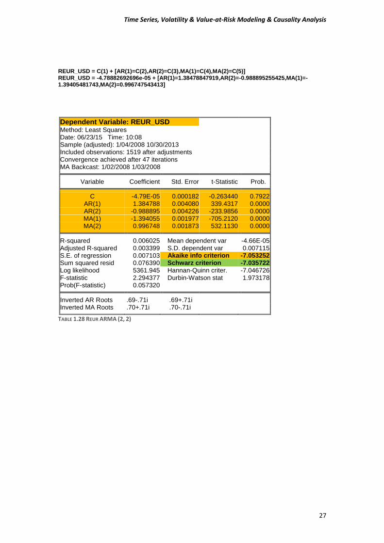
REUR_USD = C(1) + [AR(1)=C(2),AR(2)=C(3),MA(1)=C(4),MA(2)=C(5)] REUR_USD = -4.78882692696e-05 + [AR(1)=1.38478847919,AR(2)=-0.988895255425,MA(1)=-1.39405481743,MA(2)=0.996747543413]
Dependent Variable: REUR_USD Method: Least Squares Date: 06/23/15 Time: 10:08 Sample (adjusted): 1/04/2008 10/30/2013 Included observations: 1519 after adjustments Convergence achieved after 47 iterations MA Backcast: 1/02/2008 1/03/2008
Variable Coefficient Std. Error t-Statistic Prob. C -4.79E-05 0.000182 -0.263440 0.7922
AR(1) 1.384788 0.004080 339.4317 0.0000 AR(2) -0.988895 0.004226 -233.9856 0.0000 MA(1) -1.394055 0.001977 -705.2120 0.0000 MA(2) 0.996748 0.001873 532.1130 0.0000
R-squared 0.006025 Mean dependent var -4.66E-05
Adjusted R-squared 0.003399 S.D. dependent var 0.007115 S.E. of regression 0.007103 Akaike info criterion -7.053252 Sum squared resid 0.076390 Schwarz criterion -7.035722 Log likelihood 5361.945 Hannan-Quinn criter. -7.046726 F-statistic 2.294377 Durbin-Watson stat 1.973178 Prob(F-statistic) 0.057320
Inverted AR Roots .69-.71i .69+.71i
Inverted MA Roots .70+.71i .70-.71i
TABLE 1.28 REUR ARMA (2, 2)
Time Series, Volatility & Value-at-Risk Modeling & Causality Analysis
28
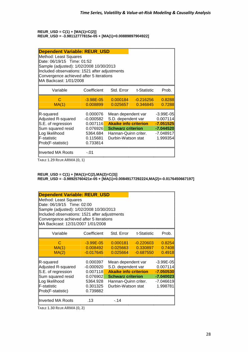
REUR_USD = C(1) + [MA(1)=C(2)] REUR_USD = -3.98112777815e-05 + [MA(1)=0.00889897904922]
Dependent Variable: REUR_USD Method: Least Squares Date: 06/19/15 Time: 01:52 Sample (adjusted): 1/02/2008 10/30/2013 Included observations: 1521 after adjustments Convergence achieved after 5 iterations MA Backcast: 1/01/2008
Variable Coefficient Std. Error t-Statistic Prob. C -3.98E-05 0.000184 -0.216256 0.8288
MA(1) 0.008899 0.025657 0.346845 0.7288 R-squared 0.000076 Mean dependent var -3.99E-05
Adjusted R-squared -0.000582 S.D. dependent var 0.007114 S.E. of regression 0.007116 Akaike info criterion -7.051525 Sum squared resid 0.076926 Schwarz criterion -7.044520 Log likelihood 5364.684 Hannan-Quinn criter. -7.048917 F-statistic 0.115681 Durbin-Watson stat 1.999354 Prob(F-statistic) 0.733814
Inverted MA Roots -.01
TABLE 1.29 REUR ARMA (0, 1)
REUR_USD = C(1) + [MA(1)=C(2),MA(2)=C(3)] REUR_USD = -3.98925760421e-05 + [MA(1)=0.00849177292224,MA(2)=-0.0176450667197]
Dependent Variable: REUR_USD Method: Least Squares Date: 06/19/15 Time: 02:00 Sample (adjusted): 1/02/2008 10/30/2013 Included observations: 1521 after adjustments Convergence achieved after 5 iterations MA Backcast: 12/31/2007 1/01/2008
Variable Coefficient Std. Error t-Statistic Prob. C -3.99E-05 0.000181 -0.220603 0.8254
MA(1) 0.008492 0.025663 0.330897 0.7408 MA(2) -0.017645 0.025664 -0.687550 0.4918
R-squared 0.000397 Mean dependent var -3.99E-05
Adjusted R-squared -0.000920 S.D. dependent var 0.007114 S.E. of regression 0.007118 Akaike info criterion -7.050530 Sum squared resid 0.076902 Schwarz criterion -7.040023 Log likelihood 5364.928 Hannan-Quinn criter. -7.046619 F-statistic 0.301325 Durbin-Watson stat 1.998781 Prob(F-statistic) 0.739882
Inverted MA Roots .13 -.14
TABLE 1.30 REUR ARMA (0, 2)
Time Series, Volatility & Value-at-Risk Modeling & Causality Analysis
29
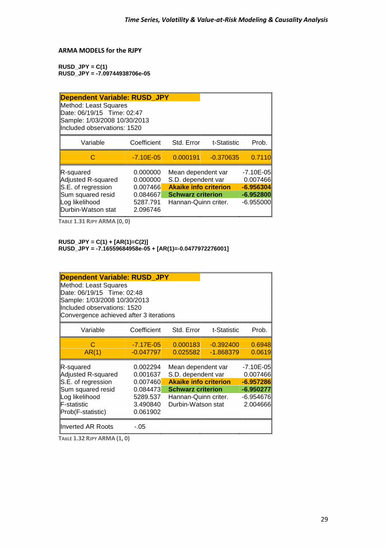
ARMA MODELS for the RJPY RUSD_JPY = C(1) RUSD_JPY = -7.09744938706e-05
Dependent Variable: RUSD_JPY Method: Least Squares Date: 06/19/15 Time: 02:47 Sample: 1/03/2008 10/30/2013 Included observations: 1520
Variable Coefficient Std. Error t-Statistic Prob. C -7.10E-05 0.000191 -0.370635 0.7110 R-squared 0.000000 Mean dependent var -7.10E-05
Adjusted R-squared 0.000000 S.D. dependent var 0.007466 S.E. of regression 0.007466 Akaike info criterion -6.956304 Sum squared resid 0.084667 Schwarz criterion -6.952800 Log likelihood 5287.791 Hannan-Quinn criter. -6.955000 Durbin-Watson stat 2.096746
TABLE 1.31 RJPY ARMA (0, 0) RUSD_JPY = C(1) + [AR(1)=C(2)] RUSD_JPY = -7.16559684958e-05 + [AR(1)=-0.0477972276001]
Dependent Variable: RUSD_JPY Method: Least Squares Date: 06/19/15 Time: 02:48 Sample: 1/03/2008 10/30/2013 Included observations: 1520 Convergence achieved after 3 iterations
Variable Coefficient Std. Error t-Statistic Prob. C -7.17E-05 0.000183 -0.392400 0.6948
AR(1) -0.047797 0.025582 -1.868379 0.0619 R-squared 0.002294 Mean dependent var -7.10E-05
Adjusted R-squared 0.001637 S.D. dependent var 0.007466 S.E. of regression 0.007460 Akaike info criterion -6.957286 Sum squared resid 0.084473 Schwarz criterion -6.950277 Log likelihood 5289.537 Hannan-Quinn criter. -6.954676 F-statistic 3.490840 Durbin-Watson stat 2.004666 Prob(F-statistic) 0.061902
Inverted AR Roots -.05
TABLE 1.32 RJPY ARMA (1, 0)
Time Series, Volatility & Value-at-Risk Modeling & Causality Analysis
30
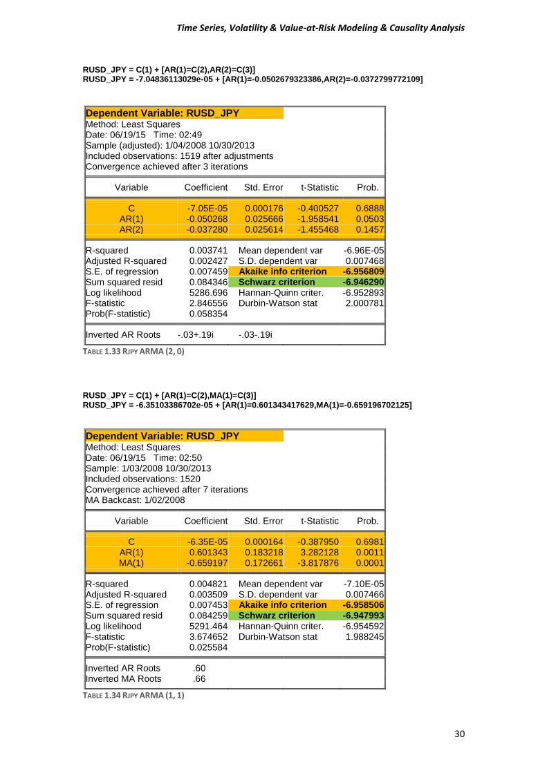
RUSD_JPY = C(1) + [AR(1)=C(2),AR(2)=C(3)] RUSD_JPY = -7.04836113029e-05 + [AR(1)=-0.0502679323386,AR(2)=-0.0372799772109]
Dependent Variable: RUSD_JPY Method: Least Squares Date: 06/19/15 Time: 02:49 Sample (adjusted): 1/04/2008 10/30/2013 Included observations: 1519 after adjustments Convergence achieved after 3 iterations
Variable Coefficient Std. Error t-Statistic Prob. C -7.05E-05 0.000176 -0.400527 0.6888
AR(1) -0.050268 0.025666 -1.958541 0.0503 AR(2) -0.037280 0.025614 -1.455468 0.1457
R-squared 0.003741 Mean dependent var -6.96E-05
Adjusted R-squared 0.002427 S.D. dependent var 0.007468 S.E. of regression 0.007459 Akaike info criterion -6.956809 Sum squared resid 0.084346 Schwarz criterion -6.946290 Log likelihood 5286.696 Hannan-Quinn criter. -6.952893 F-statistic 2.846556 Durbin-Watson stat 2.000781 Prob(F-statistic) 0.058354
Inverted AR Roots -.03+.19i -.03-.19i
TABLE 1.33 RJPY ARMA (2, 0)
RUSD_JPY = C(1) + [AR(1)=C(2),MA(1)=C(3)] RUSD_JPY = -6.35103386702e-05 + [AR(1)=0.601343417629,MA(1)=-0.659196702125]
Dependent Variable: RUSD_JPY Method: Least Squares Date: 06/19/15 Time: 02:50 Sample: 1/03/2008 10/30/2013 Included observations: 1520 Convergence achieved after 7 iterations MA Backcast: 1/02/2008
Variable Coefficient Std. Error t-Statistic Prob. C -6.35E-05 0.000164 -0.387950 0.6981
AR(1) 0.601343 0.183218 3.282128 0.0011 MA(1) -0.659197 0.172661 -3.817876 0.0001
R-squared 0.004821 Mean dependent var -7.10E-05
Adjusted R-squared 0.003509 S.D. dependent var 0.007466 S.E. of regression 0.007453 Akaike info criterion -6.958506 Sum squared resid 0.084259 Schwarz criterion -6.947993 Log likelihood 5291.464 Hannan-Quinn criter. -6.954592 F-statistic 3.674652 Durbin-Watson stat 1.988245 Prob(F-statistic) 0.025584
Inverted AR Roots .60
Inverted MA Roots .66
TABLE 1.34 RJPY ARMA (1, 1)
Time Series, Volatility & Value-at-Risk Modeling & Causality Analysis
31
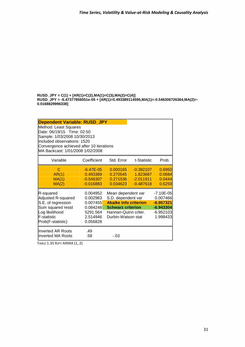
RUSD_JPY = C(1) + [AR(1)=C(2),MA(1)=C(3),MA(2)=C(4)] RUSD_JPY = -6.47377856051e-05 + [AR(1)=0.493389114595,MA(1)=-0.546306726364,MA(2)=-0.0168829996338]
Dependent Variable: RUSD_JPY Method: Least Squares Date: 06/19/15 Time: 02:50 Sample: 1/03/2008 10/30/2013 Included observations: 1520 Convergence achieved after 10 iterations MA Backcast: 1/01/2008 1/02/2008
Variable Coefficient Std. Error t-Statistic Prob. C -6.47E-05 0.000165 -0.392107 0.6950
AR(1) 0.493389 0.270545 1.823687 0.0684 MA(1) -0.546307 0.271536 -2.011911 0.0444 MA(2) -0.016883 0.034623 -0.487618 0.6259
R-squared 0.004952 Mean dependent var -7.10E-05
Adjusted R-squared 0.002983 S.D. dependent var 0.007466 S.E. of regression 0.007455 Akaike info criterion -6.957321 Sum squared resid 0.084248 Schwarz criterion -6.943304 Log likelihood 5291.564 Hannan-Quinn criter. -6.952103 F-statistic 2.514946 Durbin-Watson stat 1.998433 Prob(F-statistic) 0.056828
Inverted AR Roots .49
Inverted MA Roots .58 -.03
TABLE 1.35 RJPY ARMA (1, 2)
Time Series, Volatility & Value-at-Risk Modeling & Causality Analysis
32
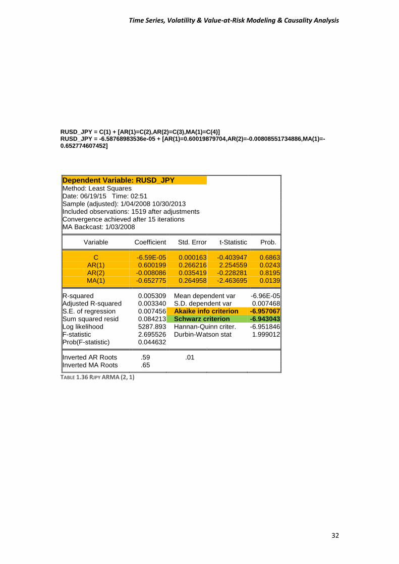
RUSD_JPY = C(1) + [AR(1)=C(2),AR(2)=C(3),MA(1)=C(4)] RUSD_JPY = -6.58768983536e-05 + [AR(1)=0.60019879704,AR(2)=-0.00808551734886,MA(1)=-0.652774607452]
Dependent Variable: RUSD_JPY Method: Least Squares Date: 06/19/15 Time: 02:51 Sample (adjusted): 1/04/2008 10/30/2013 Included observations: 1519 after adjustments Convergence achieved after 15 iterations MA Backcast: 1/03/2008
Variable Coefficient Std. Error t-Statistic Prob. C -6.59E-05 0.000163 -0.403947 0.6863
AR(1) 0.600199 0.266216 2.254559 0.0243 AR(2) -0.008086 0.035419 -0.228281 0.8195 MA(1) -0.652775 0.264958 -2.463695 0.0139
R-squared 0.005309 Mean dependent var -6.96E-05
Adjusted R-squared 0.003340 S.D. dependent var 0.007468 S.E. of regression 0.007456 Akaike info criterion -6.957067 Sum squared resid 0.084213 Schwarz criterion -6.943043 Log likelihood 5287.893 Hannan-Quinn criter. -6.951846 F-statistic 2.695526 Durbin-Watson stat 1.999012 Prob(F-statistic) 0.044632
Inverted AR Roots .59 .01
Inverted MA Roots .65
TABLE 1.36 RJPY ARMA (2, 1)
Time Series, Volatility & Value-at-Risk Modeling & Causality Analysis
33
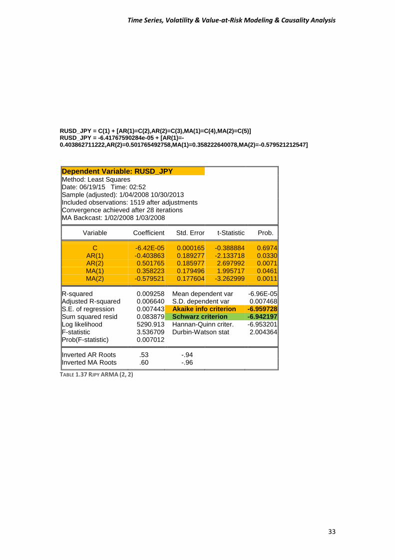
RUSD_JPY = C(1) + [AR(1)=C(2),AR(2)=C(3),MA(1)=C(4),MA(2)=C(5)] RUSD_JPY = -6.41767590284e-05 + [AR(1)=-0.403862711222,AR(2)=0.501765492758,MA(1)=0.358222640078,MA(2)=-0.579521212547]
Dependent Variable: RUSD_JPY Method: Least Squares Date: 06/19/15 Time: 02:52 Sample (adjusted): 1/04/2008 10/30/2013 Included observations: 1519 after adjustments Convergence achieved after 28 iterations MA Backcast: 1/02/2008 1/03/2008
Variable Coefficient Std. Error t-Statistic Prob. C -6.42E-05 0.000165 -0.388884 0.6974
AR(1) -0.403863 0.189277 -2.133718 0.0330 AR(2) 0.501765 0.185977 2.697992 0.0071 MA(1) 0.358223 0.179496 1.995717 0.0461 MA(2) -0.579521 0.177604 -3.262999 0.0011
R-squared 0.009258 Mean dependent var -6.96E-05
Adjusted R-squared 0.006640 S.D. dependent var 0.007468 S.E. of regression 0.007443 Akaike info criterion -6.959728 Sum squared resid 0.083879 Schwarz criterion -6.942197 Log likelihood 5290.913 Hannan-Quinn criter. -6.953201 F-statistic 3.536709 Durbin-Watson stat 2.004364 Prob(F-statistic) 0.007012
Inverted AR Roots .53 -.94
Inverted MA Roots .60 -.96
TABLE 1.37 RJPY ARMA (2, 2)
Time Series, Volatility & Value-at-Risk Modeling & Causality Analysis
34
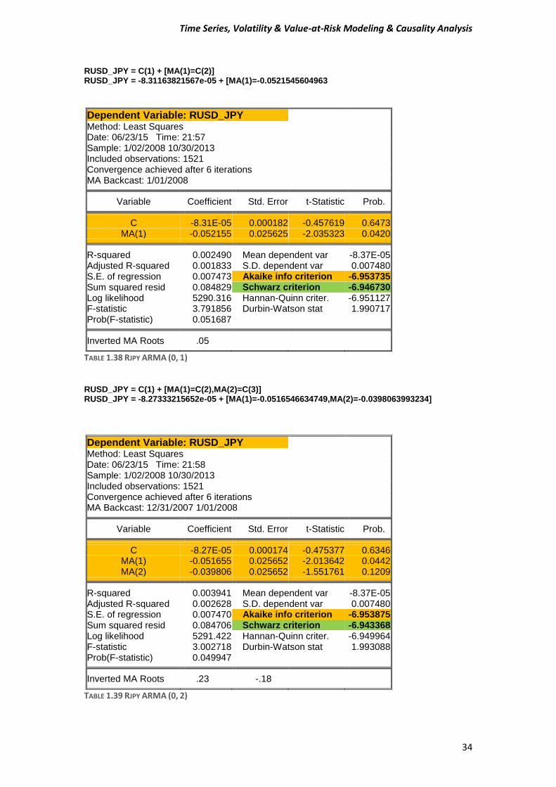
RUSD_JPY = C(1) + [MA(1)=C(2)] RUSD_JPY = -8.31163821567e-05 + [MA(1)=-0.0521545604963
Dependent Variable: RUSD_JPY Method: Least Squares Date: 06/23/15 Time: 21:57 Sample: 1/02/2008 10/30/2013 Included observations: 1521 Convergence achieved after 6 iterations MA Backcast: 1/01/2008
Variable Coefficient Std. Error t-Statistic Prob. C -8.31E-05 0.000182 -0.457619 0.6473
MA(1) -0.052155 0.025625 -2.035323 0.0420 R-squared 0.002490 Mean dependent var -8.37E-05
Adjusted R-squared 0.001833 S.D. dependent var 0.007480 S.E. of regression 0.007473 Akaike info criterion -6.953735 Sum squared resid 0.084829 Schwarz criterion -6.946730 Log likelihood 5290.316 Hannan-Quinn criter. -6.951127 F-statistic 3.791856 Durbin-Watson stat 1.990717 Prob(F-statistic) 0.051687
Inverted MA Roots .05
TABLE 1.38 RJPY ARMA (0, 1) RUSD_JPY = C(1) + [MA(1)=C(2),MA(2)=C(3)] RUSD_JPY = -8.27333215652e-05 + [MA(1)=-0.0516546634749,MA(2)=-0.0398063993234]
Dependent Variable: RUSD_JPY Method: Least Squares Date: 06/23/15 Time: 21:58 Sample: 1/02/2008 10/30/2013 Included observations: 1521 Convergence achieved after 6 iterations MA Backcast: 12/31/2007 1/01/2008
Variable Coefficient Std. Error t-Statistic Prob. C -8.27E-05 0.000174 -0.475377 0.6346
MA(1) -0.051655 0.025652 -2.013642 0.0442 MA(2) -0.039806 0.025652 -1.551761 0.1209
R-squared 0.003941 Mean dependent var -8.37E-05
Adjusted R-squared 0.002628 S.D. dependent var 0.007480 S.E. of regression 0.007470 Akaike info criterion -6.953875 Sum squared resid 0.084706 Schwarz criterion -6.943368 Log likelihood 5291.422 Hannan-Quinn criter. -6.949964 F-statistic 3.002718 Durbin-Watson stat 1.993088 Prob(F-statistic) 0.049947
Inverted MA Roots .23 -.18
TABLE 1.39 RJPY ARMA (0, 2)
Time Series, Volatility & Value-at-Risk Modeling & Causality Analysis
35
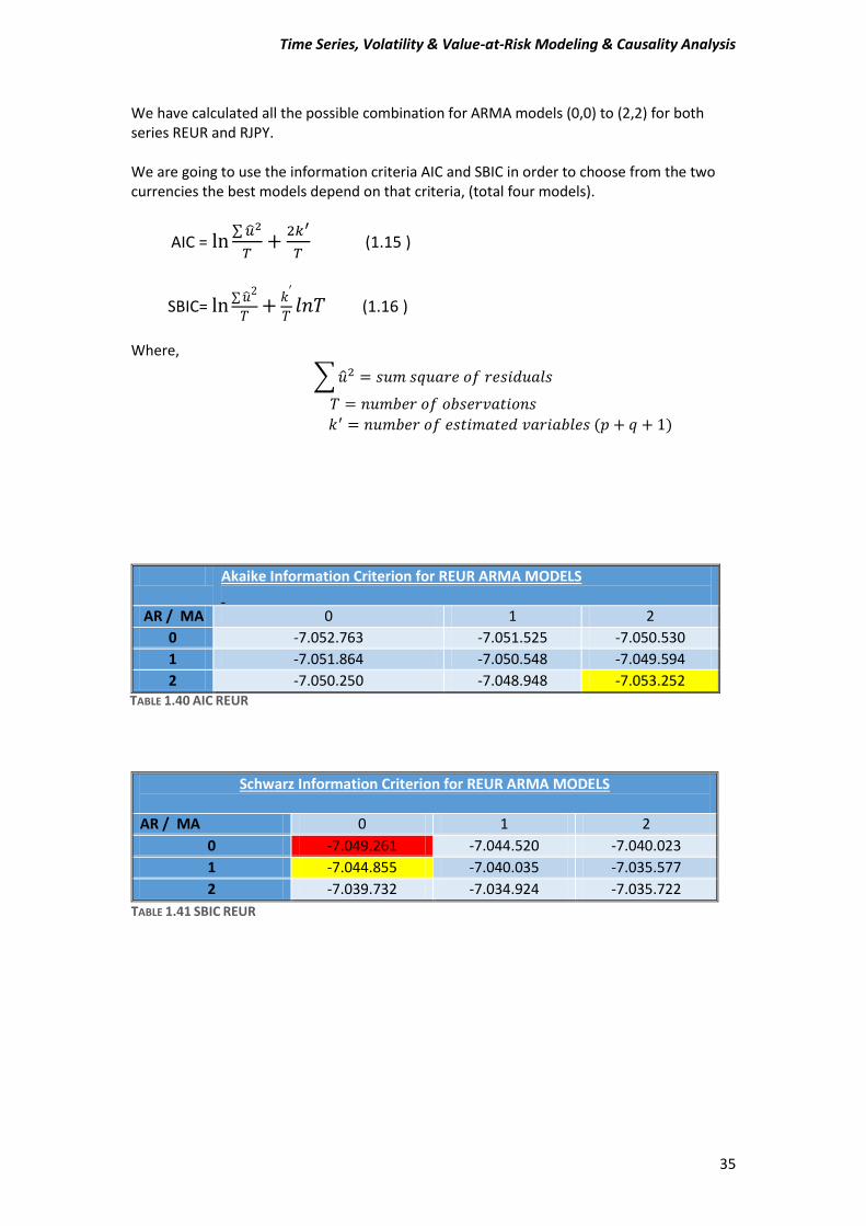
We have calculated all the possible combination for ARMA models (0,0) to (2,2) for both series REUR and RJPY. We are going to use the information criteria AIC and SBIC in order to choose from the two currencies the best models depend on that criteria, (total four models).
AIC = ln∑ 𝑢2
𝑇+
2𝑘′
𝑇 (1.15 )
SBIC= ln∑ �̂�2
𝑇+
𝑘′
𝑇𝑙𝑛𝑇 (1.16 )
Where,
∑ �̂�2 = 𝑠𝑢𝑚 𝑠𝑞𝑢𝑎𝑟𝑒 𝑜𝑓 𝑟𝑒𝑠𝑖𝑑𝑢𝑎𝑙𝑠
𝑇 = 𝑛𝑢𝑚𝑏𝑒𝑟 𝑜𝑓 𝑜𝑏𝑠𝑒𝑟𝑣𝑎𝑡𝑖𝑜𝑛𝑠
𝑘′ = 𝑛𝑢𝑚𝑏𝑒𝑟 𝑜𝑓 𝑒𝑠𝑡𝑖𝑚𝑎𝑡𝑒𝑑 𝑣𝑎𝑟𝑖𝑎𝑏𝑙𝑒𝑠 (𝑝 + 𝑞 + 1)
Schwarz Information Criterion for REUR ARMA MODELS
AR / MA 0 1 2
0 -7.049.261 -7.044.520 -7.040.023
1 -7.044.855 -7.040.035 -7.035.577
2 -7.039.732 -7.034.924 -7.035.722
TABLE 1.41 SBIC REUR
Akaike Information Criterion for REUR ARMA MODELS
AR / MA 0 1 2
0 -7.052.763 -7.051.525 -7.050.530
1 -7.051.864 -7.050.548 -7.049.594
2 -7.050.250 -7.048.948 -7.053.252 TABLE 1.40 AIC REUR
Time Series, Volatility & Value-at-Risk Modeling & Causality Analysis
36
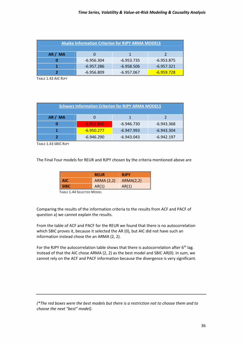
Akaike Information Criterion for RJPY ARMA MODELS
AR / MA 0 1 2
0 -6.956.304 -6.953.735 -6.953.875
1 -6.957.286 -6.958.506 -6.957.321
2 -6.956.809 -6.957.067 -6.959.728
TABLE 1.42 AIC RJPY
Schwarz Information Criterion for RJPY ARMA MODELS
AR / MA 0 1 2
0 -6.952.800 -6.946.730 -6.943.368
1 -6.950.277 -6.947.993 -6.943.304
2 -6.946.290 -6.943.043 -6.942.197
TABLE 1.43 SBIC RJPY
The Final Four models for REUR and RJPY chosen by the criteria mentioned above are Comparing the results of the information criteria to the results from ACF and PACF of question a) we cannot explain the results. From the table of ACF and PACF for the REUR we found that there is no autocorrelation which SBIC proves it, because it selected the AR (0), but AIC did not have such an information instead chose the an ARMA (2, 2). For the RJPY the autocorrelation table shows that there is autocorrelation after 6th lag. Instead of that the AIC chose ARMA (2, 2) as the best model and SBIC AR(0). In sum, we cannot rely on the ACF and PACF information because the divergence is very significant.
(*The red boxes were the best models but there is a restriction not to choose them and to choose the next “best” model).
REUR RJPY
AIC ARMA (2,2) ARMA(2,2)
SIBC AR(1) AR(1) TABLE 1.44 SELECTED MODEL
Time Series, Volatility & Value-at-Risk Modeling & Causality Analysis
37
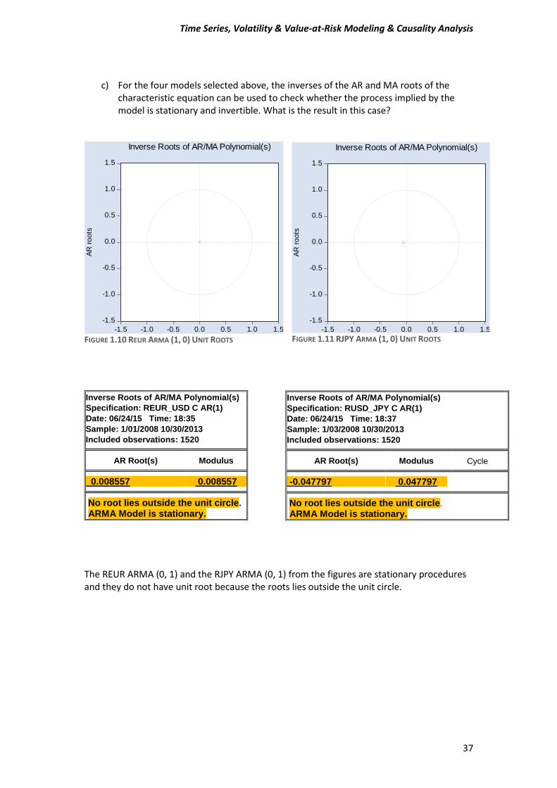
c) For the four models selected above, the inverses of the AR and MA roots of the
characteristic equation can be used to check whether the process implied by the model is stationary and invertible. What is the result in this case?
Inverse Roots of AR/MA Polynomial(s)
Specification: REUR_USD C AR(1)
Date: 06/24/15 Time: 18:35
Sample: 1/01/2008 10/30/2013
Included observations: 1520 AR Root(s) Modulus 0.008557 0.008557 No root lies outside the unit circle.
ARMA Model is stationary.
The REUR ARMA (0, 1) and the RJPY ARMA (0, 1) from the figures are stationary procedures and they do not have unit root because the roots lies outside the unit circle.
Inverse Roots of AR/MA Polynomial(s)
Specification: RUSD_JPY C AR(1)
Date: 06/24/15 Time: 18:37
Sample: 1/03/2008 10/30/2013
Included observations: 1520 AR Root(s) Modulus Cycle -0.047797 0.047797 No root lies outside the unit circle.
ARMA Model is stationary.
-1.5
-1.0
-0.5
0.0
0.5
1.0
1.5
-1.5 -1.0 -0.5 0.0 0.5 1.0 1.5
AR
ro
ots
Inverse Roots of AR/MA Polynomial(s)
-1.5
-1.0
-0.5
0.0
0.5
1.0
1.5
-1.5 -1.0 -0.5 0.0 0.5 1.0 1.5
AR
ro
ots
Inverse Roots of AR/MA Polynomial(s)
FIGURE 1.10 REUR ARMA (1, 0) UNIT ROOTS FIGURE 1.11 RJPY ARMA (1, 0) UNIT ROOTS
Time Series, Volatility & Value-at-Risk Modeling & Causality Analysis
38
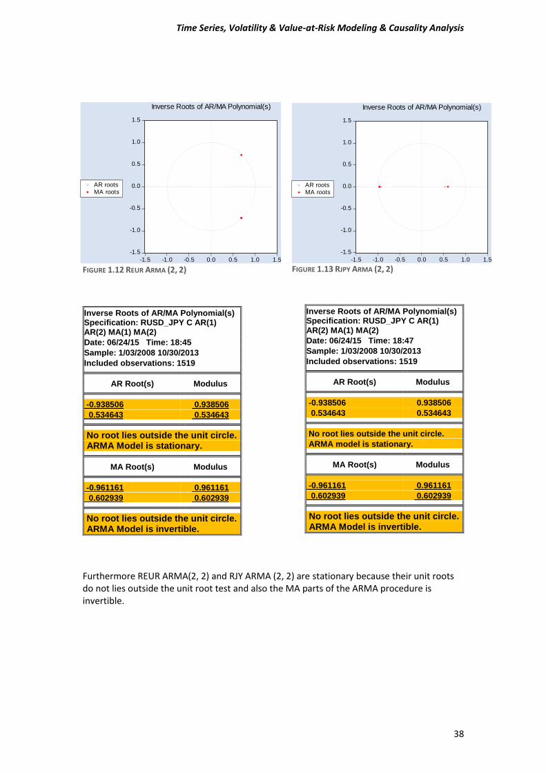
Furthermore REUR ARMA(2, 2) and RJY ARMA (2, 2) are stationary because their unit roots do not lies outside the unit root test and also the MA parts of the ARMA procedure is invertible.
Inverse Roots of AR/MA Polynomial(s) Specification: RUSD_JPY C AR(1) AR(2) MA(1) MA(2)
Date: 06/24/15 Time: 18:45
Sample: 1/03/2008 10/30/2013
Included observations: 1519 AR Root(s) Modulus -0.938506 0.938506
0.534643 0.534643 No root lies outside the unit circle.
ARMA Model is stationary. MA Root(s) Modulus -0.961161 0.961161
0.602939 0.602939 No root lies outside the unit circle.
ARMA Model is invertible.
Inverse Roots of AR/MA Polynomial(s) Specification: RUSD_JPY C AR(1) AR(2) MA(1) MA(2)
Date: 06/24/15 Time: 18:47
Sample: 1/03/2008 10/30/2013
Included observations: 1519 AR Root(s) Modulus -0.938506 0.938506
0.534643 0.534643 No root lies outside the unit circle.
ARMA model is stationary. MA Root(s) Modulus -0.961161 0.961161
0.602939 0.602939 No root lies outside the unit circle.
ARMA Model is invertible.
-1.5
-1.0
-0.5
0.0
0.5
1.0
1.5
-1.5 -1.0 -0.5 0.0 0.5 1.0 1.5
AR roots
MA roots
Inverse Roots of AR/MA Polynomial(s)
-1.5
-1.0
-0.5
0.0
0.5
1.0
1.5
-1.5 -1.0 -0.5 0.0 0.5 1.0 1.5
AR roots
MA roots
Inverse Roots of AR/MA Polynomial(s)
FIGURE 1.12 REUR ARMA (2, 2) FIGURE 1.13 RJPY ARMA (2, 2)
Time Series, Volatility & Value-at-Risk Modeling & Causality Analysis
39
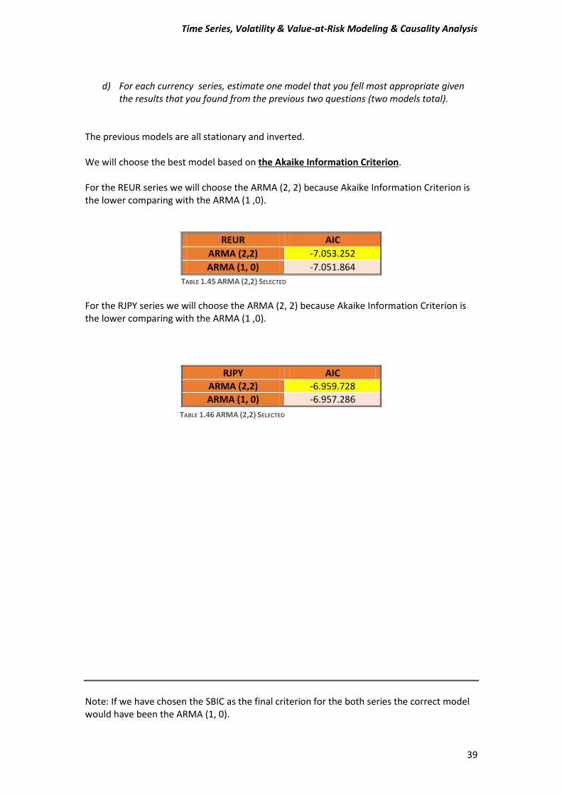
d) For each currency series, estimate one model that you fell most appropriate given
the results that you found from the previous two questions (two models total). The previous models are all stationary and inverted. We will choose the best model based on the Akaike Information Criterion. For the REUR series we will choose the ARMA (2, 2) because Akaike Information Criterion is the lower comparing with the ARMA (1 ,0).
For the RJPY series we will choose the ARMA (2, 2) because Akaike Information Criterion is the lower comparing with the ARMA (1 ,0).
Note: If we have chosen the SBIC as the final criterion for the both series the correct model would have been the ARMA (1, 0).
REUR AIC
ARMA (2,2) -7.053.252
ARMA (1, 0) -7.051.864
TABLE 1.45 ARMA (2,2) SELECTED
RJPY AIC
ARMA (2,2) -6.959.728
ARMA (1, 0) -6.957.286
TABLE 1.46 ARMA (2,2) SELECTED
Time Series, Volatility & Value-at-Risk Modeling & Causality Analysis
40
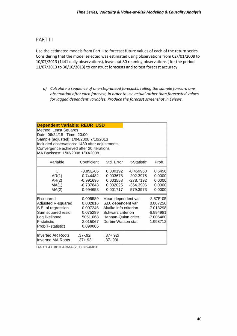
PART III Use the estimated models from Part II to forecast future values of each of the return series. Considering that the model selected was estimated using observations from 02//01/2008 to 10/07/2013 (1441 daily observations), leave out 80 reaming observations ( for the period 11/07/2013 to 30/10/2013) to construct forecasts and to test forecast accuracy.
a) Calculate a sequence of one-step-ahead forecasts, rolling the sample forward one observation after each forecast, in order to use actual rather than forecasted values for lagged dependent variables. Produce the forecast screenshot in Eviews.
Dependent Variable: REUR_USD
Method: Least Squares Date: 06/24/15 Time: 20:00 Sample (adjusted): 1/04/2008 7/10/2013 Included observations: 1439 after adjustments Convergence achieved after 20 iterations MA Backcast: 1/02/2008 1/03/2008
Variable Coefficient Std. Error t-Statistic Prob. C -8.85E-05 0.000192 -0.459960 0.6456
AR(1) 0.744482 0.003678 202.3975 0.0000 AR(2) -0.991695 0.003558 -278.7192 0.0000 MA(1) -0.737843 0.002025 -364.3906 0.0000 MA(2) 0.994653 0.001717 579.3973 0.0000
R-squared 0.005589 Mean dependent var -8.87E-05
Adjusted R-squared 0.002816 S.D. dependent var 0.007256 S.E. of regression 0.007246 Akaike info criterion -7.013298 Sum squared resid 0.075289 Schwarz criterion -6.994981 Log likelihood 5051.068 Hannan-Quinn criter. -7.006460 F-statistic 2.015067 Durbin-Watson stat 1.998712 Prob(F-statistic) 0.090005
Inverted AR Roots .37-.92i .37+.92i
Inverted MA Roots .37+.93i .37-.93i
TABLE 1.47 REUR ARMA (2, 2) IN SAMPLE
Time Series, Volatility & Value-at-Risk Modeling & Causality Analysis
41
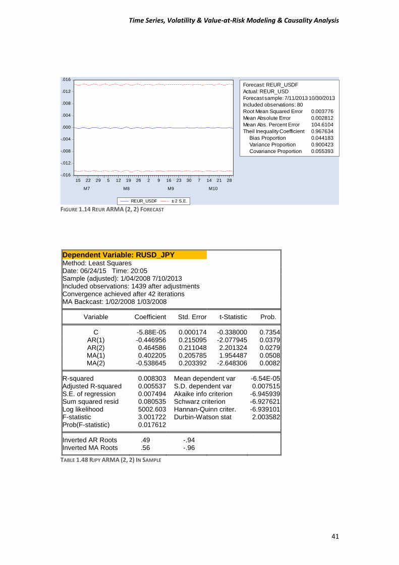
FIGURE 1.14 REUR ARMA (2, 2) FORECAST
Dependent Variable: RUSD_JPY
Method: Least Squares Date: 06/24/15 Time: 20:05 Sample (adjusted): 1/04/2008 7/10/2013 Included observations: 1439 after adjustments Convergence achieved after 42 iterations MA Backcast: 1/02/2008 1/03/2008
Variable Coefficient Std. Error t-Statistic Prob. C -5.88E-05 0.000174 -0.338000 0.7354
AR(1) -0.446956 0.215095 -2.077945 0.0379 AR(2) 0.464586 0.211048 2.201324 0.0279 MA(1) 0.402205 0.205785 1.954487 0.0508 MA(2) -0.538645 0.203392 -2.648306 0.0082
R-squared 0.008303 Mean dependent var -6.54E-05
Adjusted R-squared 0.005537 S.D. dependent var 0.007515 S.E. of regression 0.007494 Akaike info criterion -6.945939 Sum squared resid 0.080535 Schwarz criterion -6.927621 Log likelihood 5002.603 Hannan-Quinn criter. -6.939101 F-statistic 3.001722 Durbin-Watson stat 2.003582 Prob(F-statistic) 0.017612
Inverted AR Roots .49 -.94
Inverted MA Roots .56 -.96
TABLE 1.48 RJPY ARMA (2, 2) IN SAMPLE
-.016
-.012
-.008
-.004
.000
.004
.008
.012
.016
15 22 29 5 12 19 26 2 9 16 23 30 7 14 21 28
M7 M8 M9 M10
REUR_USDF ± 2 S.E.
Forecast: REUR_USDF
Actual: REUR_USD
Forecast sample: 7/11/2013 10/30/2013
Included observations: 80
Root Mean Squared Error 0.003776
Mean Absolute Error 0.002812
Mean Abs. Percent Error 104.6104
Theil Inequality Coefficient 0.967634
Bias Proportion 0.044183
Variance Proportion 0.900423
Covariance Proportion 0.055393
Time Series, Volatility & Value-at-Risk Modeling & Causality Analysis
42
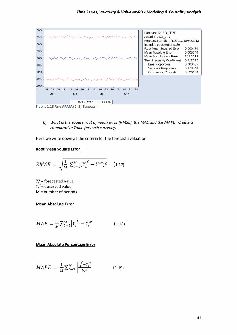
FIGURE 1.15 RJPY ARMA (2, 2) FORECAST
b) What is the square root of mean error (RMSE), the MAE and the MAPE? Create a comparative Table for each currency.
Here we write down all the criteria for the forecast evaluation. Root Mean Square Error
𝑅𝑀𝑆𝐸 = √1
𝑀 ∑ (𝑌𝑡
𝑓− 𝑌𝑡
𝛼)2𝑀𝑡=1 (1.17)
𝑌𝑡
𝑓= forecasted value
𝑌𝑡𝛼= observed value
M = number of periods
Mean Absolute Error
𝑀𝐴𝐸 =1
𝑀∑ |𝑌𝑡
𝑓− 𝑌𝑡
𝛼|𝑀𝑡=1 (1.18)
Mean Absolute Percentage Error
𝑀𝐴𝑃𝐸 = 1
𝑀∑ |
𝑌𝑡𝑓
−𝑌𝑡𝛼
𝑌𝑡𝛼 |𝑀
𝑡=1 (1.19)
-.020
-.015
-.010
-.005
.000
.005
.010
.015
.020
15 22 29 5 12 19 26 2 9 16 23 30 7 14 21 28
M7 M8 M9 M10
RUSD_JPYF ± 2 S.E.
Forecast: RUSD_JPYF
Actual: RUSD_JPY
Forecast sample: 7/11/2013 10/30/2013
Included observations: 80
Root Mean Squared Error 0.006470
Mean Absolute Error 0.005140
Mean Abs. Percent Error 101.1219
Theil Inequality Coefficient 0.912072
Bias Proportion 0.000405
Variance Proportion 0.873446
Covariance Proportion 0.126150
Time Series, Volatility & Value-at-Risk Modeling & Causality Analysis
43
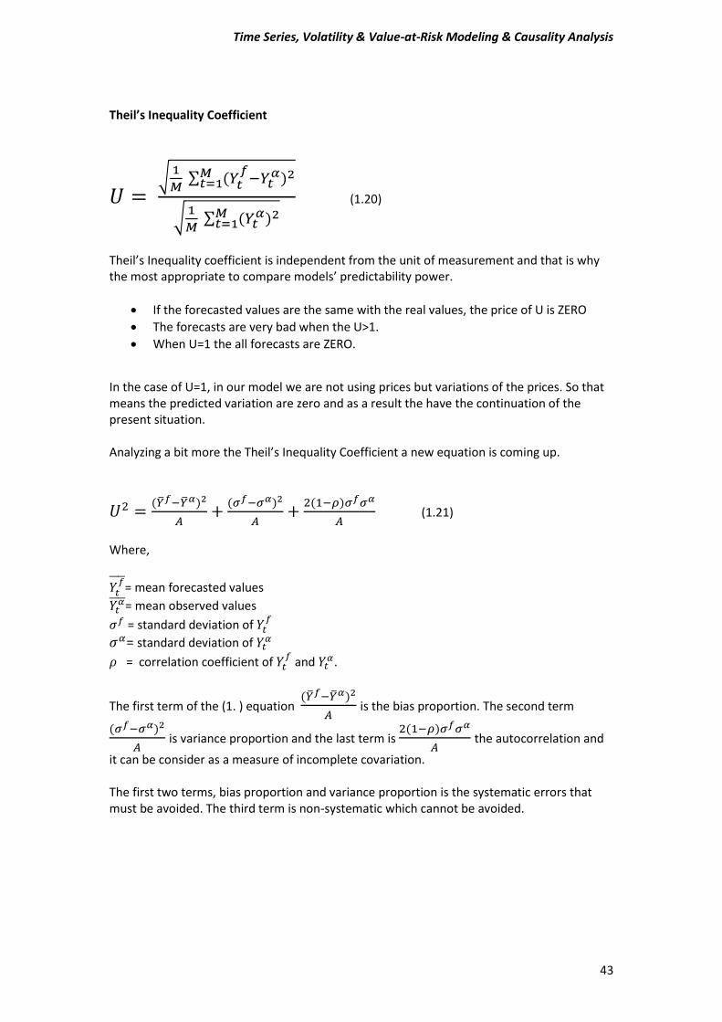
Theil’s Inequality Coefficient
𝑈 = √
1
𝑀 ∑ (𝑌𝑡
𝑓−𝑌𝑡
𝛼)2𝑀𝑡=1
√1
𝑀 ∑ (𝑌𝑡
𝛼)2𝑀𝑡=1
(1.20)
Theil’s Inequality coefficient is independent from the unit of measurement and that is why the most appropriate to compare models’ predictability power.
If the forecasted values are the same with the real values, the price of U is ZERO
The forecasts are very bad when the U>1.
When U=1 the all forecasts are ZERO.
In the case of U=1, in our model we are not using prices but variations of the prices. So that means the predicted variation are zero and as a result the have the continuation of the present situation. Analyzing a bit more the Theil’s Inequality Coefficient a new equation is coming up.
𝑈2 =(�̅�𝑓−�̅�𝛼)2
𝛢+
(𝜎𝑓−𝜎𝛼)2
𝛢+
2(1−𝜌)𝜎𝑓𝜎𝛼
𝛢 (1.21)
Where,
𝑌𝑡𝑓̅̅̅̅
= mean forecasted values
𝑌𝑡𝛼̅̅ ̅̅ = mean observed values
𝜎𝑓 = standard deviation of 𝑌𝑡𝑓
𝜎𝛼= standard deviation of 𝑌𝑡𝛼
𝜌 = correlation coefficient of 𝑌𝑡𝑓
and 𝑌𝑡𝛼.
The first term of the (1. ) equation (�̅�𝑓−�̅�𝛼)2
𝛢 is the bias proportion. The second term
(𝜎𝑓−𝜎𝛼)2
𝛢 is variance proportion and the last term is
2(1−𝜌)𝜎𝑓𝜎𝛼
𝛢 the autocorrelation and
it can be consider as a measure of incomplete covariation. The first two terms, bias proportion and variance proportion is the systematic errors that must be avoided. The third term is non-systematic which cannot be avoided.
Time Series, Volatility & Value-at-Risk Modeling & Causality Analysis
44
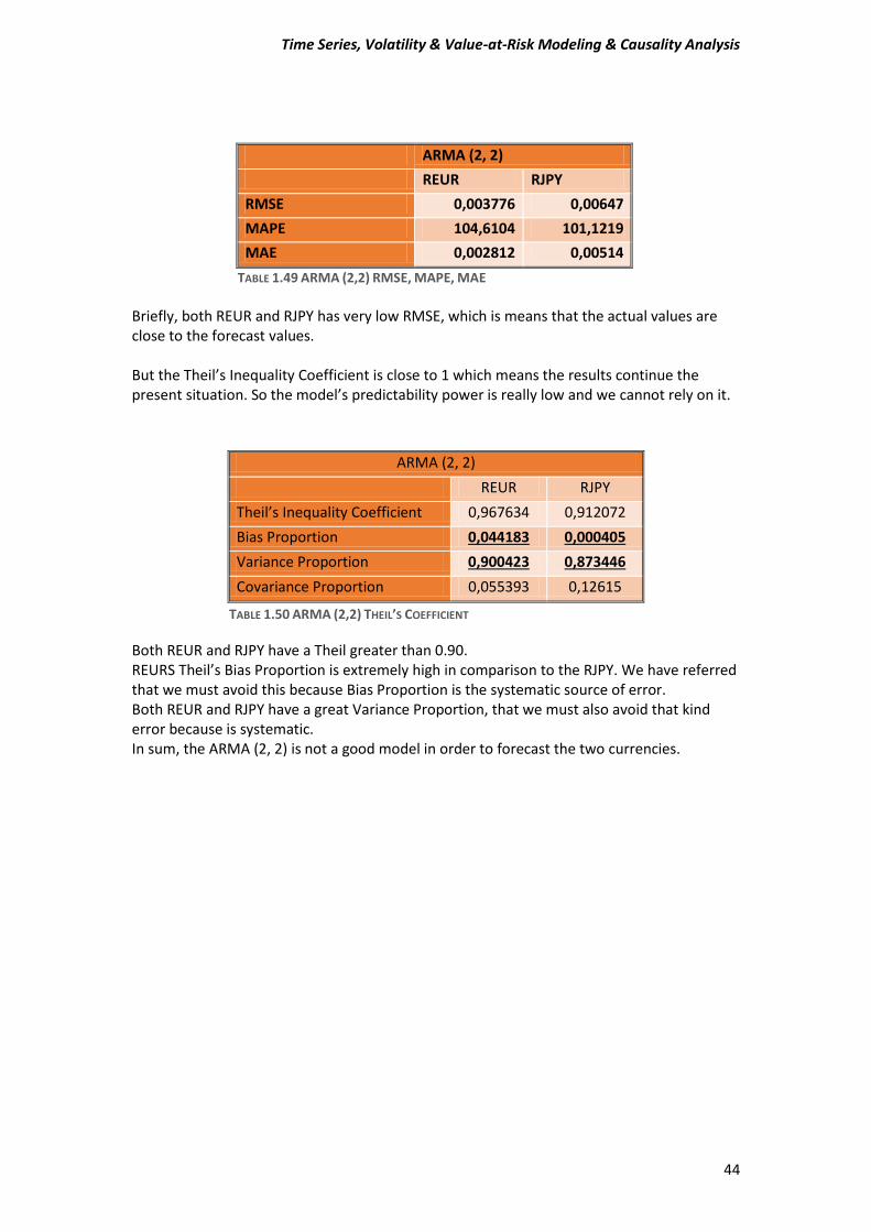
ARMA (2, 2)
REUR RJPY
RMSE 0,003776 0,00647
MAPE 104,6104 101,1219
MAE 0,002812 0,00514
TABLE 1.49 ARMA (2,2) RMSE, MAPE, MAE
Briefly, both REUR and RJPY has very low RMSE, which is means that the actual values are close to the forecast values. But the Theil’s Inequality Coefficient is close to 1 which means the results continue the present situation. So the model’s predictability power is really low and we cannot rely on it. Both REUR and RJPY have a Theil greater than 0.90. REURS Theil’s Bias Proportion is extremely high in comparison to the RJPY. We have referred that we must avoid this because Bias Proportion is the systematic source of error. Both REUR and RJPY have a great Variance Proportion, that we must also avoid that kind error because is systematic. In sum, the ARMA (2, 2) is not a good model in order to forecast the two currencies.
ARMA (2, 2)
REUR RJPY
Theil’s Inequality Coefficient 0,967634 0,912072
Bias Proportion 0,044183 0,000405
Variance Proportion 0,900423 0,873446
Covariance Proportion 0,055393 0,12615
TABLE 1.50 ARMA (2,2) THEIL’S COEFFICIENT
Time Series, Volatility & Value-at-Risk Modeling & Causality Analysis
45
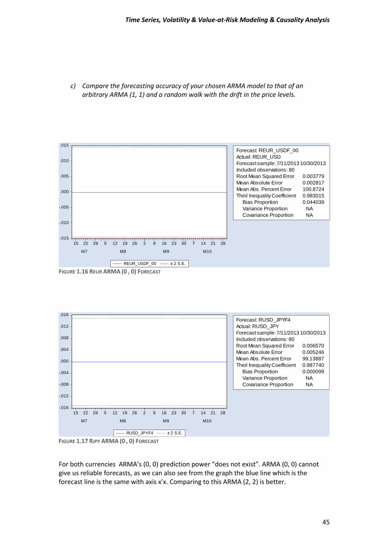
c) Compare the forecasting accuracy of your chosen ARMA model to that of an arbitrary ARMA (1, 1) and a random walk with the drift in the price levels.
FIGURE 1.16 REUR ARMA (0 , 0) FORECAST
For both currencies ARMA’s (0, 0) prediction power “does not exist”. ARMA (0, 0) cannot give us reliable forecasts, as we can also see from the graph the blue line which is the forecast line is the same with axis x’x. Comparing to this ARMA (2, 2) is better.
-.015
-.010
-.005
.000
.005
.010
.015
15 22 29 5 12 19 26 2 9 16 23 30 7 14 21 28
M7 M8 M9 M10
REUR_USDF_00 ± 2 S.E.
Forecast: REUR_USDF_00
Actual: REUR_USD
Forecast sample: 7/11/2013 10/30/2013
Included observations: 80
Root Mean Squared Error 0.003779
Mean Absolute Error 0.002817
Mean Abs. Percent Error 100.8724
Theil Inequality Coefficient 0.983015
Bias Proportion 0.044039
Variance Proportion NA
Covariance Proportion NA
-.016
-.012
-.008
-.004
.000
.004
.008
.012
.016
15 22 29 5 12 19 26 2 9 16 23 30 7 14 21 28
M7 M8 M9 M10
RUSD_JPYF4 ± 2 S.E.
Forecast: RUSD_JPYF4
Actual: RUSD_JPY
Forecast sample: 7/11/2013 10/30/2013
Included observations: 80
Root Mean Squared Error 0.006570
Mean Absolute Error 0.005246
Mean Abs. Percent Error 99.13887
Theil Inequality Coefficient 0.987740
Bias Proportion 0.000099
Variance Proportion NA
Covariance Proportion NA
FIGURE 1.17 RJPY ARMA (0 , 0) FORECAST
Time Series, Volatility & Value-at-Risk Modeling & Causality Analysis
46
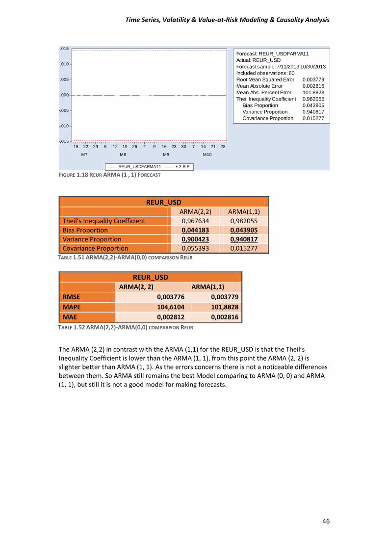
FIGURE 1.18 REUR ARMA (1 , 1) FORECAST
The ARMA (2,2) in contrast with the ARMA (1,1) for the REUR_USD is that the Theil’s Inequality Coefficient is lower than the ARMA (1, 1), from this point the ARMA (2, 2) is slighter better than ARMA (1, 1). As the errors concerns there is not a noticeable differences between them. So ARMA still remains the best Model comparing to ARMA (0, 0) and ARMA (1, 1), but still it is not a good model for making forecasts.
-.015
-.010
-.005
.000
.005
.010
.015
15 22 29 5 12 19 26 2 9 16 23 30 7 14 21 28
M7 M8 M9 M10
REUR_USDFARMA11 ± 2 S.E.
Forecast: REUR_USDFARMA11
Actual: REUR_USD
Forecast sample: 7/11/2013 10/30/2013
Included observations: 80
Root Mean Squared Error 0.003779
Mean Absolute Error 0.002816
Mean Abs. Percent Error 101.8828
Theil Inequality Coefficient 0.982055
Bias Proportion 0.043905
Variance Proportion 0.940817
Covariance Proportion 0.015277
REUR_USD ARMA(2,2) ARMA(1,1)
Theil’s Inequality Coefficient 0,967634 0,982055
Bias Proportion 0,044183 0,043905
Variance Proportion 0,900423 0,940817
Covariance Proportion 0,055393 0,015277 TABLE 1.51 ARMA(2,2)-ARMA(0,0) COMPARISON REUR
REUR_USD
ARMA(2, 2) ARMA(1,1)
RMSE 0,003776 0,003779
MAPE 104,6104 101,8828
MAE 0,002812 0,002816
TABLE 1.52 ARMA(2,2)-ARMA(0,0) COMPARISON REUR
Time Series, Volatility & Value-at-Risk Modeling & Causality Analysis
47
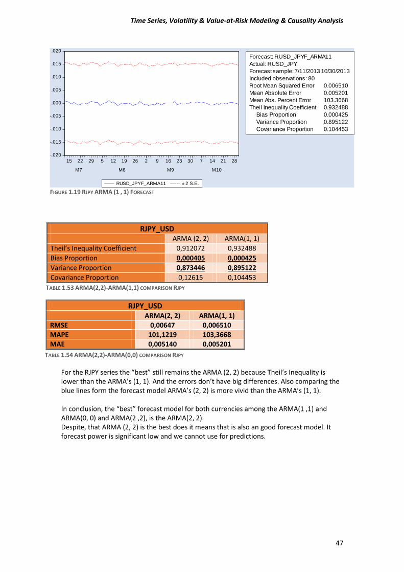
For the RJPY series the “best” still remains the ARMA (2, 2) because Theil’s Inequality is lower than the ARMA’s (1, 1). And the errors don’t have big differences. Also comparing the blue lines form the forecast model ARMA’s (2, 2) is more vivid than the ARMA’s (1, 1). In conclusion, the “best” forecast model for both currencies among the ARMA(1 ,1) and ARMA(0, 0) and ARMA(2 ,2), is the ARMA(2, 2). Despite, that ARMA (2, 2) is the best does it means that is also an good forecast model. It forecast power is significant low and we cannot use for predictions.
RJPY_USD
ARMA (2, 2) ARMA(1, 1)
Theil’s Inequality Coefficient 0,912072 0,932488
Bias Proportion 0,000405 0,000425
Variance Proportion 0,873446 0,895122
Covariance Proportion 0,12615 0,104453
TABLE 1.53 ARMA(2,2)-ARMA(1,1) COMPARISON RJPY
RJPY_USD
ARMA(2, 2) ARMA(1, 1)
RMSE 0,00647 0,006510
MAPE 101,1219 103,3668
MAE 0,005140 0,005201
TABLE 1.54 ARMA(2,2)-ARMA(0,0) COMPARISON RJPY
-.020
-.015
-.010
-.005
.000
.005
.010
.015
.020
15 22 29 5 12 19 26 2 9 16 23 30 7 14 21 28
M7 M8 M9 M10
RUSD_JPYF_ARMA11 ± 2 S.E.
Forecast: RUSD_JPYF_ARMA11
Actual: RUSD_JPY
Forecast sample: 7/11/2013 10/30/2013
Included observations: 80
Root Mean Squared Error 0.006510
Mean Absolute Error 0.005201
Mean Abs. Percent Error 103.3668
Theil Inequality Coefficient 0.932488
Bias Proportion 0.000425
Variance Proportion 0.895122
Covariance Proportion 0.104453
FIGURE 1.19 RJPY ARMA (1 , 1) FORECAST
Time Series, Volatility & Value-at-Risk Modeling & Causality Analysis
48
SECTION II VOLATILITY MODELING & VALUE-AT-RISK
PART I
A) Before estimating a GARCH-type model, test for ARCH effects in stock returns. Compute the Engle test for ARCH effects to make sure that this class of models is appropriate for the data. Estimate an ARMA (1, 1) model and then test or the presence of ARCH in the residuals. Use five lags for the tests and comment on the Engle ARCH test (F- and x^2 version) for the presence of ARCH in each of the stock market returns.
ARCH rank (p) MODEL
𝜎𝑡2 = 𝛼0 + 𝛼1𝑢𝑡−1
2 + 𝛼2𝑢𝑡−22 + ⋯ + 𝛼𝑝𝑢𝑡−𝑝
2 (2.1)
Now the function (2.1) can be generalized, thus the conditional variance 𝜎𝑡2 to be an
additional a function of itself with time lag. To be more specific: GARCH rank (p) MODEL
𝜎𝑡2 = 𝛼0 + 𝛼1𝑢𝑡−1
2 + 𝛼2𝑢𝑡−22 + ⋯ + 𝛼𝑝𝑢𝑡−𝑝
2 + 𝛾1𝜎𝑡−12 + ⋯ + 𝛾𝑞𝜎𝑡−𝑞
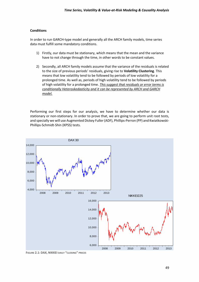
2 (2.2) The function (2.2) is known as Generalized Autoregressive Conditional Heteroskedasticity or GARCH model. So here we have to estimate a GARCH-type model for our data. Few words for our data We are going to use daily “closing” prices of the DAX/German Stock Index and the NIKKEI225/Japanese index series. There are total of 1523 observations running from 31/12/2007 to 30/10/2013. DAX_30= Deutcher Aktien-Indice as we know is a German Stock Index. It is traded on the Frankfurt Stock Exchange which is the biggest stock exchange in Germany. DAX measures the development of the 30 largest and best-performing companies on the German equities market and represents around 80% of the market capitalization in Germany. NIKKEI 225 It is a price-weighted index consisting of 225 prominent stocks on the Tokyo Stock Exchange. The Nikkei has been calculated since 1950 and its direction is considered an indicator of the state of the Japanese economy.
Time Series, Volatility & Value-at-Risk Modeling & Causality Analysis
49
Conditions In order to run GARCH-type model and generally all the ARCH family models, time series data must fulfill some mandatory conditions.
1) Firstly, our data must be stationary, which means that the mean and the variance have to not change through the time, in other words to be constant values.
2) Secondly, all ARCH family models assume that the variance of the residuals is related to the size of previous periods’ residuals, giving rise to Volatility Clustering. This means that low volatility tend to be followed by periods of low volatility for a prolonged time. As well as, periods of high volatility tend to be followed by periods of high volatility for a prolonged time. This suggest that residuals or error terms is conditionally Heteroskedasticity and it can be represented by ARCH and GARCH model.
Performing our first steps for our analysis, we have to determine whether our data is stationary or non-stationary. In order to prove that, we are going to perform unit root tests, and specially we will use Augmented Dickey Fuller (ADF), Phillips-Perron (PP) and Kwiatkowski-Phillips-Schmidt-Shin (KPSS) tests.
4,000
6,000
8,000
10,000
12,000
14,000
2008 2009 2010 2011 2012 2013
DAX 30
6,000
8,000
10,000
12,000
14,000
16,000
2008 2009 2010 2011 2012 2013
NIKKEI225
FIGURE 2.1: DAX, NIKKEI DAILY “CLOSING” PRICES
Time Series, Volatility & Value-at-Risk Modeling & Causality Analysis
50
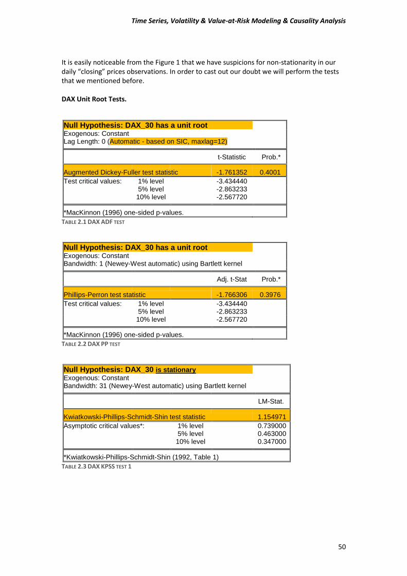
It is easily noticeable from the Figure 1 that we have suspicions for non-stationarity in our daily “closing” prices observations. In order to cast out our doubt we will perform the tests that we mentioned before. DAX Unit Root Tests.
Null Hypothesis: DAX_30 has a unit root Exogenous: Constant Lag Length: 0 (Automatic - based on SIC, maxlag=12)
t-Statistic Prob.*
Augmented Dickey-Fuller test statistic -1.761352 0.4001
Test critical values: 1% level -3.434440 5% level -2.863233 10% level -2.567720 *MacKinnon (1996) one-sided p-values.
TABLE 2.1 DAX ADF TEST
Null Hypothesis: DAX_30 has a unit root
Exogenous: Constant
Bandwidth: 1 (Newey-West automatic) using Bartlett kernel Adj. t-Stat Prob.*
Phillips-Perron test statistic -1.766306 0.3976
Test critical values: 1% level -3.434440 5% level -2.863233 10% level -2.567720
*MacKinnon (1996) one-sided p-values.
TABLE 2.2 DAX PP TEST
Null Hypothesis: DAX_30 is stationary
Exogenous: Constant
Bandwidth: 31 (Newey-West automatic) using Bartlett kernel LM-Stat.
Kwiatkowski-Phillips-Schmidt-Shin test statistic 1.154971
Asymptotic critical values*: 1% level 0.739000 5% level 0.463000 10% level 0.347000
*Kwiatkowski-Phillips-Schmidt-Shin (1992, Table 1)
TABLE 2.3 DAX KPSS TEST 1
Time Series, Volatility & Value-at-Risk Modeling & Causality Analysis
51
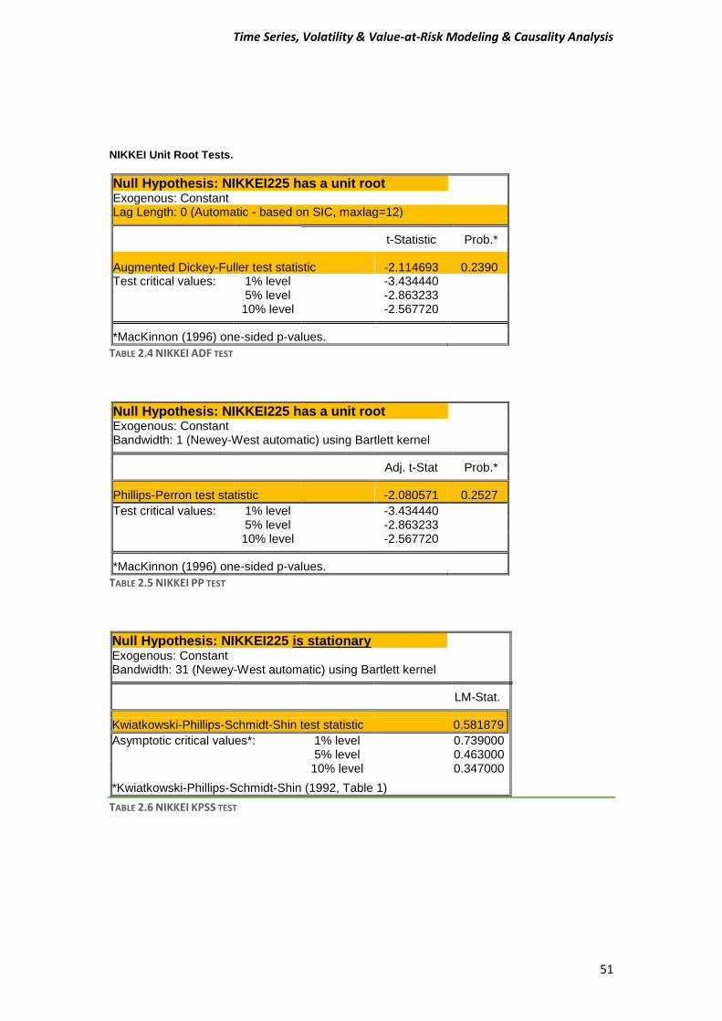
NIKKEI Unit Root Tests.
Null Hypothesis: NIKKEI225 has a unit root Exogenous: Constant Lag Length: 0 (Automatic - based on SIC, maxlag=12)
t-Statistic Prob.*
Augmented Dickey-Fuller test statistic -2.114693 0.2390 Test critical values: 1% level -3.434440
5% level -2.863233 10% level -2.567720 *MacKinnon (1996) one-sided p-values.
TABLE 2.4 NIKKEI ADF TEST
Null Hypothesis: NIKKEI225 has a unit root Exogenous: Constant Bandwidth: 1 (Newey-West automatic) using Bartlett kernel
Adj. t-Stat Prob.*
Phillips-Perron test statistic -2.080571 0.2527
Test critical values: 1% level -3.434440 5% level -2.863233 10% level -2.567720 *MacKinnon (1996) one-sided p-values.
TABLE 2.5 NIKKEI PP TEST
Null Hypothesis: NIKKEI225 is stationary
Exogenous: Constant
Bandwidth: 31 (Newey-West automatic) using Bartlett kernel LM-Stat.
Kwiatkowski-Phillips-Schmidt-Shin test statistic 0.581879
Asymptotic critical values*: 1% level 0.739000 5% level 0.463000 10% level 0.347000
*Kwiatkowski-Phillips-Schmidt-Shin (1992, Table 1)
TABLE 2.6 NIKKEI KPSS TEST
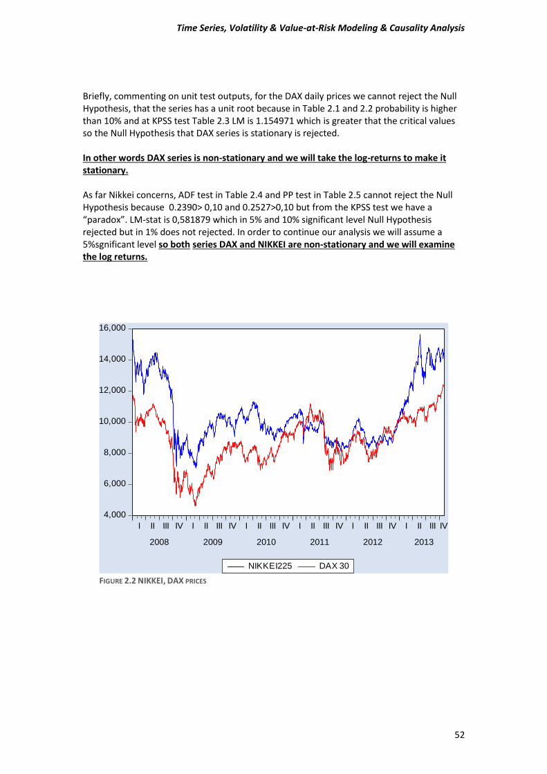
Time Series, Volatility & Value-at-Risk Modeling & Causality Analysis
52
Briefly, commenting on unit test outputs, for the DAX daily prices we cannot reject the Null Hypothesis, that the series has a unit root because in Table 2.1 and 2.2 probability is higher than 10% and at KPSS test Table 2.3 LM is 1.154971 which is greater that the critical values so the Null Hypothesis that DAX series is stationary is rejected. In other words DAX series is non-stationary and we will take the log-returns to make it stationary. As far Nikkei concerns, ADF test in Table 2.4 and PP test in Table 2.5 cannot reject the Null Hypothesis because 0.2390> 0,10 and 0.2527>0,10 but from the KPSS test we have a “paradox”. LM-stat is 0,581879 which in 5% and 10% significant level Null Hypothesis rejected but in 1% does not rejected. In order to continue our analysis we will assume a 5%sgnificant level so both series DAX and NIKKEI are non-stationary and we will examine the log returns.
4,000
6,000
8,000
10,000
12,000
14,000
16,000
I II III IV I II III IV I II III IV I II III IV I II III IV I II III IV
2008 2009 2010 2011 2012 2013
NIKKEI225 DAX 30
FIGURE 2.2 NIKKEI, DAX PRICES
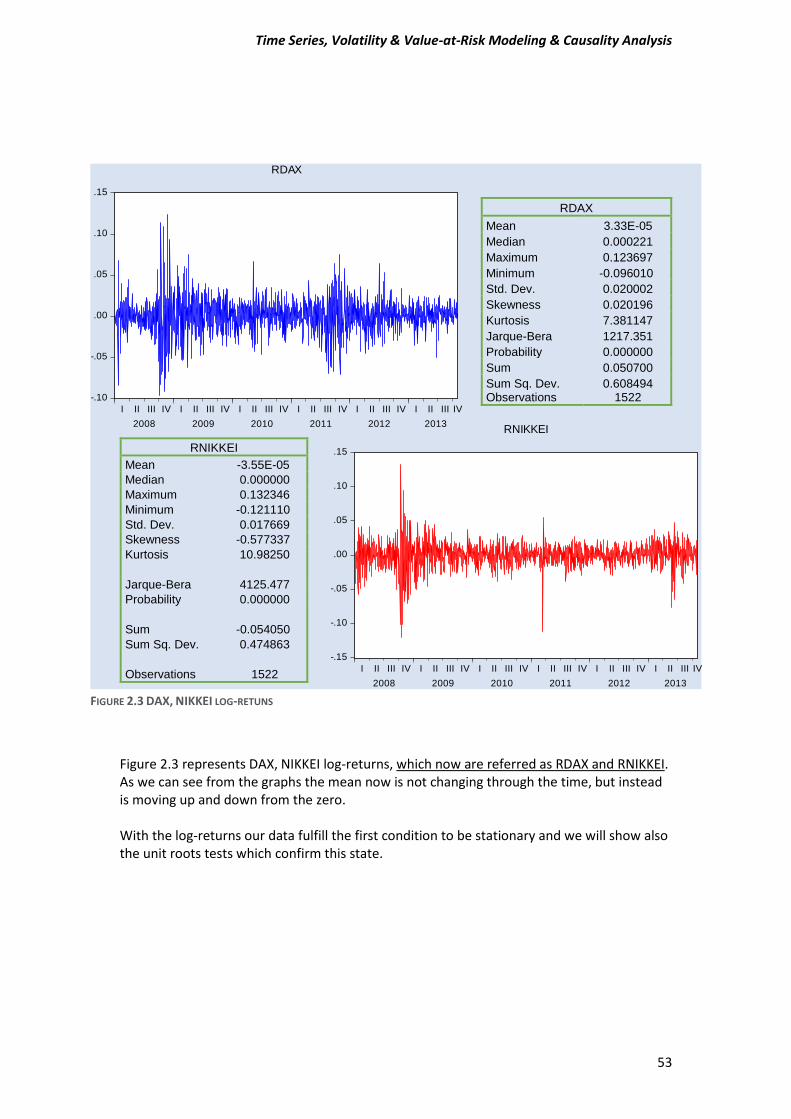
Time Series, Volatility & Value-at-Risk Modeling & Causality Analysis
53
-.10
-.05
.00
.05
.10
.15
I II III IV I II III IV I II III IV I II III IV I II III IV I II III IV
2008 2009 2010 2011 2012 2013
RDAX
-.15
-.10
-.05
.00
.05
.10
.15
I II III IV I II III IV I II III IV I II III IV I II III IV I II III IV
2008 2009 2010 2011 2012 2013
RNIKKEI
Figure 2.3 represents DAX, NIKKEI log-returns, which now are referred as RDAX and RNIKKEI. As we can see from the graphs the mean now is not changing through the time, but instead is moving up and down from the zero. With the log-returns our data fulfill the first condition to be stationary and we will show also the unit roots tests which confirm this state.
RDAX
Mean 3.33E-05
Median 0.000221
Maximum 0.123697
Minimum -0.096010
Std. Dev. 0.020002
Skewness 0.020196
Kurtosis 7.381147
Jarque-Bera 1217.351
Probability 0.000000
Sum 0.050700
Sum Sq. Dev. 0.608494 Observations 1522
RNIKKEI
Mean -3.55E-05
Median 0.000000
Maximum 0.132346
Minimum -0.121110
Std. Dev. 0.017669
Skewness -0.577337
Kurtosis 10.98250
Jarque-Bera 4125.477
Probability 0.000000
Sum -0.054050
Sum Sq. Dev. 0.474863
Observations 1522
FIGURE 2.3 DAX, NIKKEI LOG-RETUNS
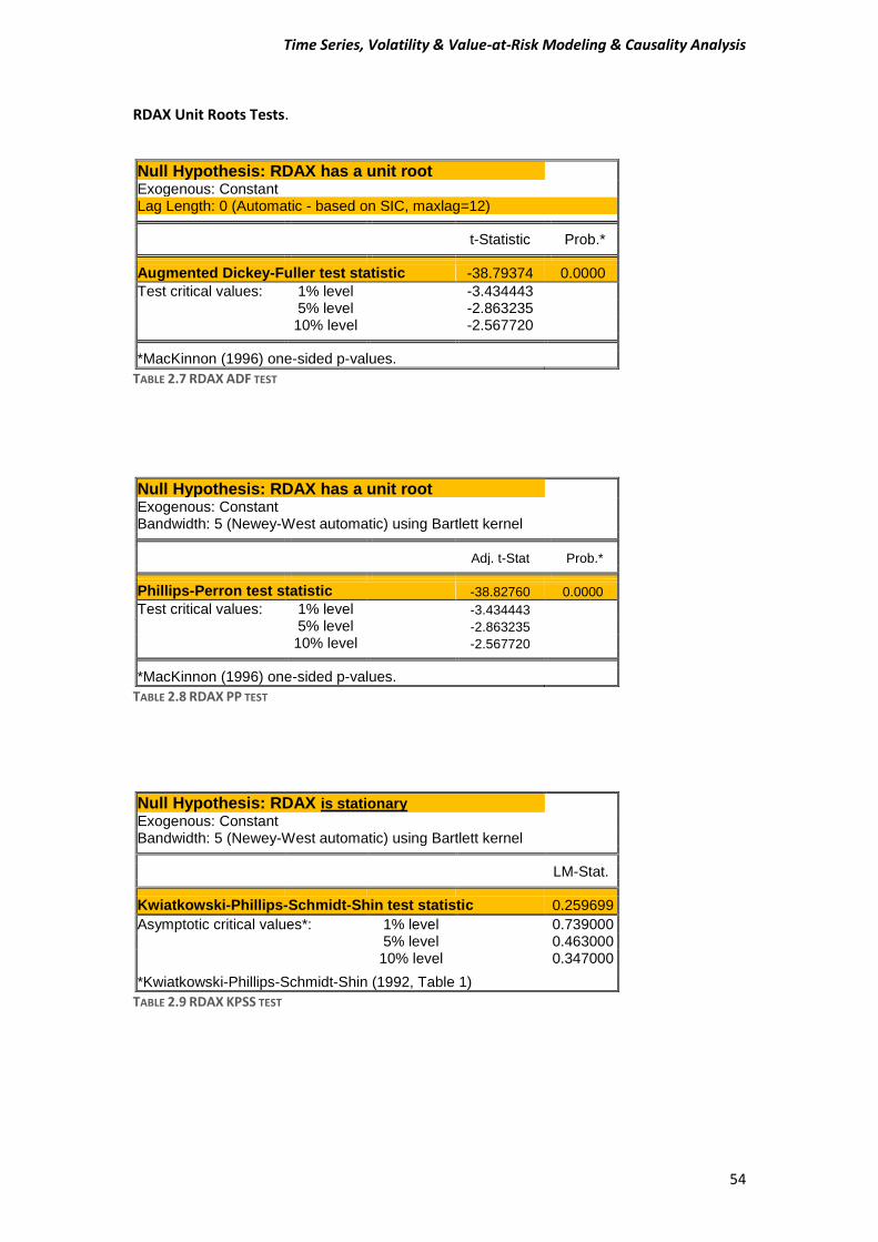
Time Series, Volatility & Value-at-Risk Modeling & Causality Analysis
54
RDAX Unit Roots Tests.
Null Hypothesis: RDAX has a unit root Exogenous: Constant Lag Length: 0 (Automatic - based on SIC, maxlag=12)
t-Statistic Prob.* Augmented Dickey-Fuller test statistic -38.79374 0.0000
Test critical values: 1% level -3.434443 5% level -2.863235 10% level -2.567720 *MacKinnon (1996) one-sided p-values.
TABLE 2.7 RDAX ADF TEST
Null Hypothesis: RDAX has a unit root
Exogenous: Constant
Bandwidth: 5 (Newey-West automatic) using Bartlett kernel Adj. t-Stat Prob.*
Phillips-Perron test statistic -38.82760 0.0000
Test critical values: 1% level -3.434443
5% level -2.863235
10% level -2.567720
*MacKinnon (1996) one-sided p-values.
TABLE 2.8 RDAX PP TEST
Null Hypothesis: RDAX is stationary Exogenous: Constant Bandwidth: 5 (Newey-West automatic) using Bartlett kernel
LM-Stat.
Kwiatkowski-Phillips-Schmidt-Shin test statistic 0.259699
Asymptotic critical values*: 1% level 0.739000 5% level 0.463000 10% level 0.347000 *Kwiatkowski-Phillips-Schmidt-Shin (1992, Table 1)
TABLE 2.9 RDAX KPSS TEST
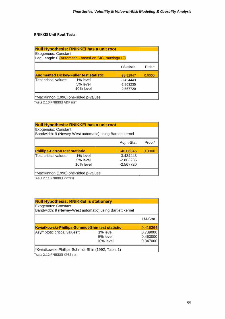
Time Series, Volatility & Value-at-Risk Modeling & Causality Analysis
55
RNIKKEI Unit Root Tests.
Null Hypothesis: RNIKKEI has a unit root
Exogenous: Constant
Lag Length: 0 (Automatic - based on SIC, maxlag=12) t-Statistic Prob.*
Augmented Dickey-Fuller test statistic -39.92947 0.0000
Test critical values: 1% level -3.434443
5% level -2.863235
10% level -2.567720
*MacKinnon (1996) one-sided p-values.
TABLE 2.10 RNIKKEI ADF TEST
Null Hypothesis: RNIKKEI has a unit root Exogenous: Constant Bandwidth: 9 (Newey-West automatic) using Bartlett kernel
Adj. t-Stat Prob.* Phillips-Perron test statistic -40.06845 0.0000
Test critical values: 1% level -3.434443 5% level -2.863235 10% level -2.567720 *MacKinnon (1996) one-sided p-values.
TABLE 2.11 RNIKKEI PP TEST
Null Hypothesis: RNIKKEI is stationary Exogenous: Constant Bandwidth: 9 (Newey-West automatic) using Bartlett kernel
LM-Stat. Kwiatkowski-Phillips-Schmidt-Shin test statistic 0.416364
Asymptotic critical values*: 1% level 0.739000 5% level 0.463000 10% level 0.347000 *Kwiatkowski-Phillips-Schmidt-Shin (1992, Table 1)
TABLE 2.12 RNIKKEI KPSS TEST
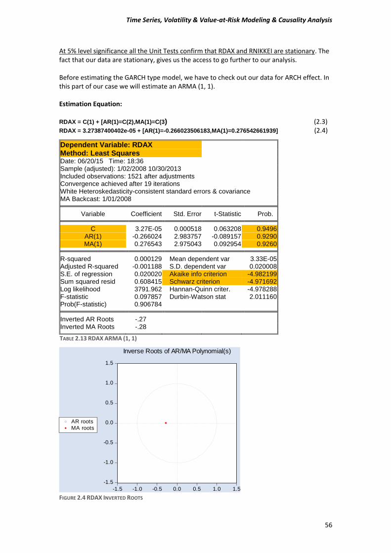
Time Series, Volatility & Value-at-Risk Modeling & Causality Analysis
56
-1.5
-1.0
-0.5
0.0
0.5
1.0
1.5
-1.5 -1.0 -0.5 0.0 0.5 1.0 1.5
AR roots
MA roots
Inverse Roots of AR/MA Polynomial(s)
FIGURE 2.4 RDAX INVERTED ROOTS
At 5% level significance all the Unit Tests confirm that RDAX and RNIKKEI are stationary. The fact that our data are stationary, gives us the access to go further to our analysis. Before estimating the GARCH type model, we have to check out our data for ARCH effect. In this part of our case we will estimate an ARMA (1, 1). Estimation Equation: RDAX = C(1) + [AR(1)=C(2),MA(1)=C(3) (2.3) RDAX = 3.27387400402e-05 + [AR(1)=-0.266023506183,MA(1)=0.276542661939] (2.4)
Dependent Variable: RDAX
Method: Least Squares Date: 06/20/15 Time: 18:36 Sample (adjusted): 1/02/2008 10/30/2013 Included observations: 1521 after adjustments Convergence achieved after 19 iterations White Heteroskedasticity-consistent standard errors & covariance MA Backcast: 1/01/2008
Variable Coefficient Std. Error t-Statistic Prob. C 3.27E-05 0.000518 0.063208 0.9496
AR(1) -0.266024 2.983757 -0.089157 0.9290 MA(1) 0.276543 2.975043 0.092954 0.9260
R-squared 0.000129 Mean dependent var 3.33E-05
Adjusted R-squared -0.001188 S.D. dependent var 0.020008 S.E. of regression 0.020020 Akaike info criterion -4.982199 Sum squared resid 0.608415 Schwarz criterion -4.971692 Log likelihood 3791.962 Hannan-Quinn criter. -4.978288 F-statistic 0.097857 Durbin-Watson stat 2.011160 Prob(F-statistic) 0.906784
Inverted AR Roots -.27
Inverted MA Roots -.28
TABLE 2.13 RDAX ARMA (1, 1)
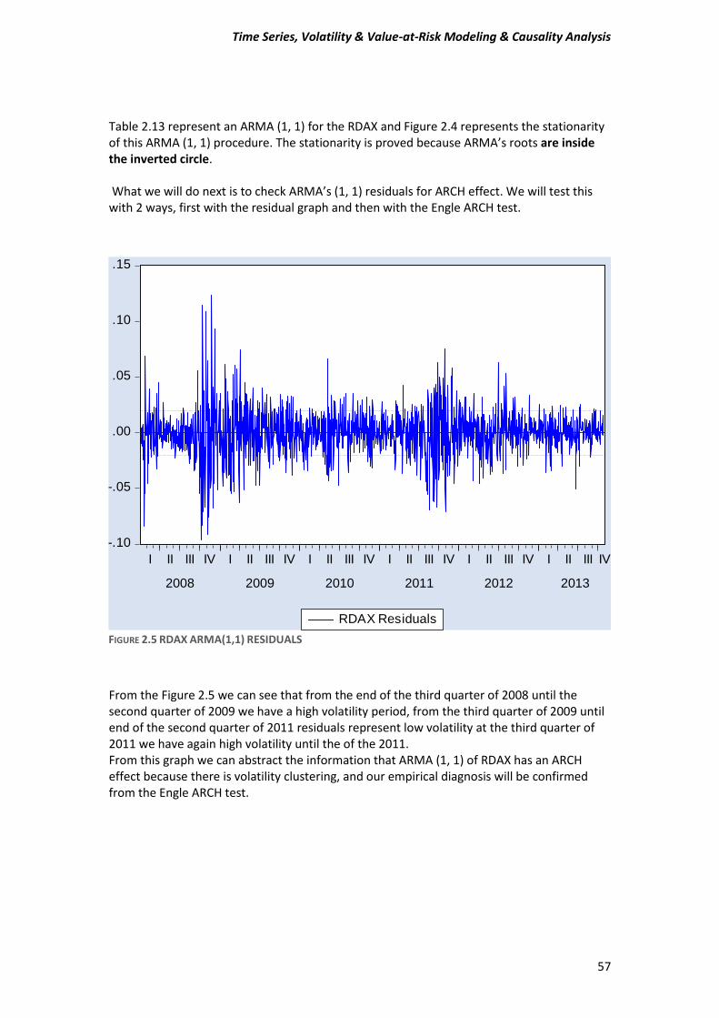
Time Series, Volatility & Value-at-Risk Modeling & Causality Analysis
57
Table 2.13 represent an ARMA (1, 1) for the RDAX and Figure 2.4 represents the stationarity of this ARMA (1, 1) procedure. The stationarity is proved because ARMA’s roots are inside the inverted circle. What we will do next is to check ARMA’s (1, 1) residuals for ARCH effect. We will test this with 2 ways, first with the residual graph and then with the Engle ARCH test.
From the Figure 2.5 we can see that from the end of the third quarter of 2008 until the second quarter of 2009 we have a high volatility period, from the third quarter of 2009 until end of the second quarter of 2011 residuals represent low volatility at the third quarter of 2011 we have again high volatility until the of the 2011. From this graph we can abstract the information that ARMA (1, 1) of RDAX has an ARCH effect because there is volatility clustering, and our empirical diagnosis will be confirmed from the Engle ARCH test.
-.10
-.05
.00
.05
.10
.15
I II III IV I II III IV I II III IV I II III IV I II III IV I II III IV
2008 2009 2010 2011 2012 2013
RDAX Residuals
FIGURE 2.5 RDAX ARMA(1,1) RESIDUALS
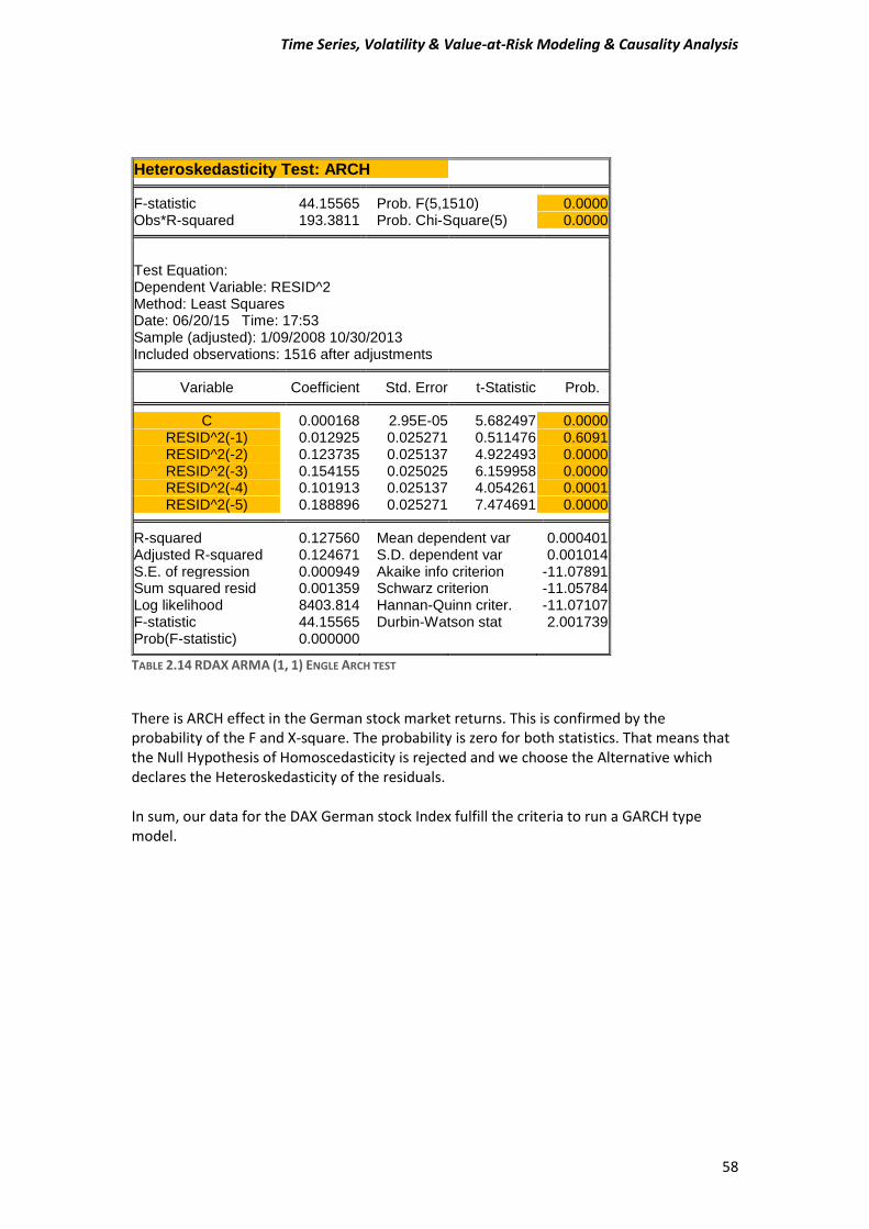
Time Series, Volatility & Value-at-Risk Modeling & Causality Analysis
58
Heteroskedasticity Test: ARCH F-statistic 44.15565 Prob. F(5,1510) 0.0000
Obs*R-squared 193.3811 Prob. Chi-Square(5) 0.0000
Test Equation: Dependent Variable: RESID^2 Method: Least Squares Date: 06/20/15 Time: 17:53 Sample (adjusted): 1/09/2008 10/30/2013 Included observations: 1516 after adjustments
Variable Coefficient Std. Error t-Statistic Prob. C 0.000168 2.95E-05 5.682497 0.0000
RESID^2(-1) 0.012925 0.025271 0.511476 0.6091 RESID^2(-2) 0.123735 0.025137 4.922493 0.0000 RESID^2(-3) 0.154155 0.025025 6.159958 0.0000 RESID^2(-4) 0.101913 0.025137 4.054261 0.0001 RESID^2(-5) 0.188896 0.025271 7.474691 0.0000
R-squared 0.127560 Mean dependent var 0.000401
Adjusted R-squared 0.124671 S.D. dependent var 0.001014 S.E. of regression 0.000949 Akaike info criterion -11.07891 Sum squared resid 0.001359 Schwarz criterion -11.05784 Log likelihood 8403.814 Hannan-Quinn criter. -11.07107 F-statistic 44.15565 Durbin-Watson stat 2.001739 Prob(F-statistic) 0.000000
TABLE 2.14 RDAX ARMA (1, 1) ENGLE ARCH TEST
There is ARCH effect in the German stock market returns. This is confirmed by the probability of the F and X-square. The probability is zero for both statistics. That means that the Null Hypothesis of Homoscedasticity is rejected and we choose the Alternative which declares the Heteroskedasticity of the residuals. In sum, our data for the DAX German stock Index fulfill the criteria to run a GARCH type model.
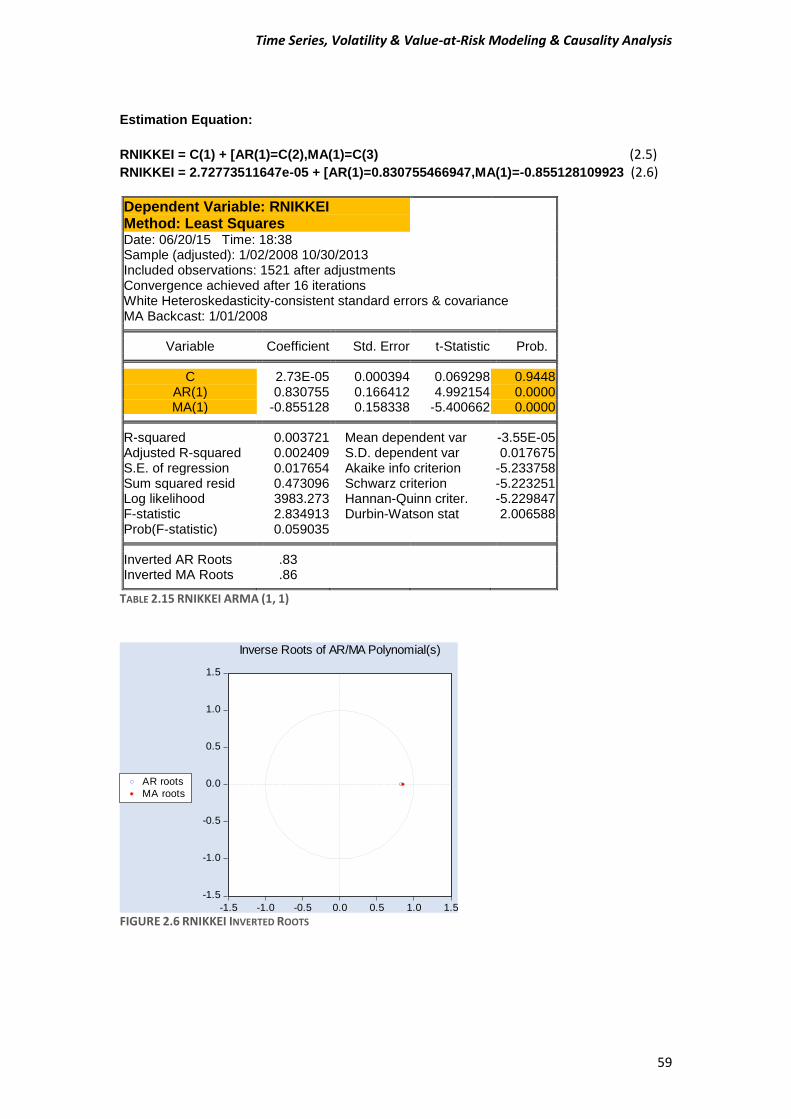
Time Series, Volatility & Value-at-Risk Modeling & Causality Analysis
59
Estimation Equation: RNIKKEI = C(1) + [AR(1)=C(2),MA(1)=C(3) (2.5) RNIKKEI = 2.72773511647e-05 + [AR(1)=0.830755466947,MA(1)=-0.855128109923 (2.6)
Dependent Variable: RNIKKEI
Method: Least Squares Date: 06/20/15 Time: 18:38 Sample (adjusted): 1/02/2008 10/30/2013 Included observations: 1521 after adjustments Convergence achieved after 16 iterations White Heteroskedasticity-consistent standard errors & covariance MA Backcast: 1/01/2008
Variable Coefficient Std. Error t-Statistic Prob. C 2.73E-05 0.000394 0.069298 0.9448
AR(1) 0.830755 0.166412 4.992154 0.0000 MA(1) -0.855128 0.158338 -5.400662 0.0000
R-squared 0.003721 Mean dependent var -3.55E-05
Adjusted R-squared 0.002409 S.D. dependent var 0.017675 S.E. of regression 0.017654 Akaike info criterion -5.233758 Sum squared resid 0.473096 Schwarz criterion -5.223251 Log likelihood 3983.273 Hannan-Quinn criter. -5.229847 F-statistic 2.834913 Durbin-Watson stat 2.006588 Prob(F-statistic) 0.059035
Inverted AR Roots .83
Inverted MA Roots .86
TABLE 2.15 RNIKKEI ARMA (1, 1)
-1.5
-1.0
-0.5
0.0
0.5
1.0
1.5
-1.5 -1.0 -0.5 0.0 0.5 1.0 1.5
AR roots
MA roots
Inverse Roots of AR/MA Polynomial(s)
FIGURE 2.6 RNIKKEI INVERTED ROOTS
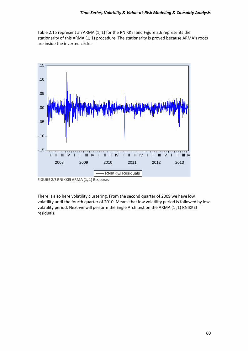
Time Series, Volatility & Value-at-Risk Modeling & Causality Analysis
60
Table 2.15 represent an ARMA (1, 1) for the RNIKKEI and Figure 2.6 represents the stationarity of this ARMA (1, 1) procedure. The stationarity is proved because ARMA’s roots are inside the inverted circle.
FIGURE 2.7 RNIKKEI ARMA (1, 1) RESIDUALS
There is also here volatility clustering. From the second quarter of 2009 we have low volatility until the fourth quarter of 2010. Means that low volatility period is followed by low volatility period. Next we will perform the Engle Arch test on the ARMA (1 ,1) RNIKKEI residuals.
-.15
-.10
-.05
.00
.05
.10
.15
I II III IV I II III IV I II III IV I II III IV I II III IV I II III IV
2008 2009 2010 2011 2012 2013
RNIKKEI Residuals
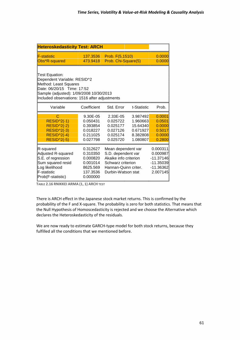
Time Series, Volatility & Value-at-Risk Modeling & Causality Analysis
61
Heteroskedasticity Test: ARCH F-statistic 137.3536 Prob. F(5,1510) 0.0000
Obs*R-squared 473.9418 Prob. Chi-Square(5) 0.0000
Test Equation: Dependent Variable: RESID^2 Method: Least Squares Date: 06/20/15 Time: 17:52 Sample (adjusted): 1/09/2008 10/30/2013 Included observations: 1516 after adjustments
Variable Coefficient Std. Error t-Statistic Prob. C 9.30E-05 2.33E-05 3.987492 0.0001
RESID^2(-1) 0.050431 0.025722 1.960663 0.0501 RESID^2(-2) 0.393854 0.025177 15.64340 0.0000 RESID^2(-3) 0.018227 0.027126 0.671927 0.5017 RESID^2(-4) 0.211025 0.025174 8.382808 0.0000 RESID^2(-5) 0.027798 0.025720 1.080807 0.2800
R-squared 0.312627 Mean dependent var 0.000311
Adjusted R-squared 0.310350 S.D. dependent var 0.000987 S.E. of regression 0.000820 Akaike info criterion -11.37146 Sum squared resid 0.001014 Schwarz criterion -11.35039 Log likelihood 8625.569 Hannan-Quinn criter. -11.36362 F-statistic 137.3536 Durbin-Watson stat 2.007145 Prob(F-statistic) 0.000000
TABLE 2.16 RNIKKEI ARMA (1, 1) ARCH TEST
There is ARCH effect in the Japanese stock market returns. This is confirmed by the probability of the F and X-square. The probability is zero for both statistics. That means that the Null Hypothesis of Homoscedasticity is rejected and we choose the Alternative which declares the Heteroskedasticity of the residuals. We are now ready to estimate GARCH-type model for both stock returns, because they fulfilled all the conditions that we mentioned before.
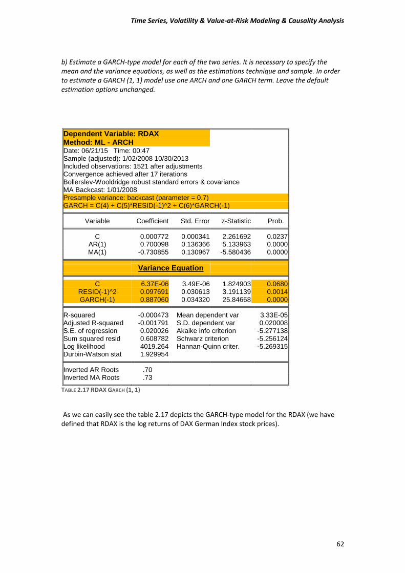
Time Series, Volatility & Value-at-Risk Modeling & Causality Analysis
62
b) Estimate a GARCH-type model for each of the two series. It is necessary to specify the mean and the variance equations, as well as the estimations technique and sample. In order to estimate a GARCH (1, 1) model use one ARCH and one GARCH term. Leave the default estimation options unchanged.
Dependent Variable: RDAX
Method: ML - ARCH Date: 06/21/15 Time: 00:47 Sample (adjusted): 1/02/2008 10/30/2013 Included observations: 1521 after adjustments Convergence achieved after 17 iterations Bollerslev-Wooldridge robust standard errors & covariance MA Backcast: 1/01/2008 Presample variance: backcast (parameter = 0.7) GARCH = C(4) + C(5)*RESID(-1)^2 + C(6)*GARCH(-1)
Variable Coefficient Std. Error z-Statistic Prob. C 0.000772 0.000341 2.261692 0.0237
AR(1) 0.700098 0.136366 5.133963 0.0000 MA(1) -0.730855 0.130967 -5.580436 0.0000
Variance Equation C 6.37E-06 3.49E-06 1.824903 0.0680
RESID(-1)^2 0.097691 0.030613 3.191139 0.0014 GARCH(-1) 0.887060 0.034320 25.84668 0.0000
R-squared -0.000473 Mean dependent var 3.33E-05
Adjusted R-squared -0.001791 S.D. dependent var 0.020008 S.E. of regression 0.020026 Akaike info criterion -5.277138 Sum squared resid 0.608782 Schwarz criterion -5.256124 Log likelihood 4019.264 Hannan-Quinn criter. -5.269315 Durbin-Watson stat 1.929954
Inverted AR Roots .70
Inverted MA Roots .73
TABLE 2.17 RDAX GARCH (1, 1)
As we can easily see the table 2.17 depicts the GARCH-type model for the RDAX (we have defined that RDAX is the log returns of DAX German Index stock prices).
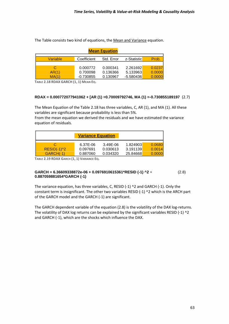
Time Series, Volatility & Value-at-Risk Modeling & Causality Analysis
63
The Table consists two kind of equations, the Mean and Variance equation.
Mean Equation
Variable Coefficient Std. Error z-Statistic Prob.
C 0.000772 0.000341 2.261692 0.0237
AR(1) 0.700098 0.136366 5.133963 0.0000 MA(1) -0.730855 0.130967 -5.580436 0.0000
TABLE 2.18 RDAX GARCH (1, 1) MEAN EQ.
RDAX = 0.000772077941062 + [AR (1) =0.70009792746, MA (1) =-0.730855189197 (2.7) The Mean Equation of the Table 2.18 has three variables, C, AR (1), and MA (1). All these variables are significant because probability is less than 5%. From the mean equation we derived the residuals and we have estimated the variance equation of residuals.
Variance Equation C 6.37E-06 3.49E-06 1.824903 0.0680
RESID(-1)^2 0.097691 0.030613 3.191139 0.0014 GARCH(-1) 0.887060 0.034320 25.84668 0.0000
TABLE 2.19 RDAX GARCH (1, 1) VARIANCE EQ. GARCH = 6.36609338872e-06 + 0.0976910615361*RESID (-1) ^2 + (2.8) 0.887059881654*GARCH (-1) The variance equation, has three variables, C, RESID (-1) ^2 and GARCH (-1). Only the constant term is insignificant. The other two variables RESID (-1) ^2 which is the ARCH part of the GARCH model and the GARCH (-1) are significant. The GARCH dependent variable of the equation (2.8) is the volatility of the DAX log-returns. The volatility of DAX log returns can be explained by the significant variables RESID (-1) ^2 and GARCH (-1), which are the shocks which influence the DAX.
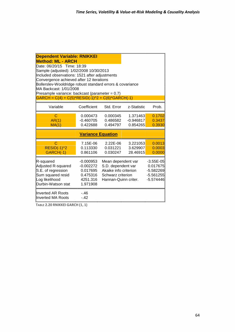
Time Series, Volatility & Value-at-Risk Modeling & Causality Analysis
64
Dependent Variable: RNIKKEI
Method: ML - ARCH Date: 06/20/15 Time: 18:39 Sample (adjusted): 1/02/2008 10/30/2013 Included observations: 1521 after adjustments Convergence achieved after 12 iterations Bollerslev-Wooldridge robust standard errors & covariance MA Backcast: 1/01/2008 Presample variance: backcast (parameter = 0.7) GARCH = C(4) + C(5)*RESID(-1)^2 + C(6)*GARCH(-1)
Variable Coefficient Std. Error z-Statistic Prob. C 0.000473 0.000345 1.371463 0.1702
AR(1) -0.460705 0.486582 -0.946817 0.3437 MA(1) 0.422688 0.494797 0.854265 0.3930
Variance Equation C 7.15E-06 2.22E-06 3.221053 0.0013
RESID(-1)^2 0.113330 0.031221 3.629907 0.0003 GARCH(-1) 0.861106 0.030247 28.46915 0.0000
R-squared -0.000953 Mean dependent var -3.55E-05
Adjusted R-squared -0.002272 S.D. dependent var 0.017675 S.E. of regression 0.017695 Akaike info criterion -5.582269 Sum squared resid 0.475316 Schwarz criterion -5.561255 Log likelihood 4251.316 Hannan-Quinn criter. -5.574446 Durbin-Watson stat 1.971908
Inverted AR Roots -.46
Inverted MA Roots -.42
TABLE 2.20 RNIKKEI GARCH (1, 1)
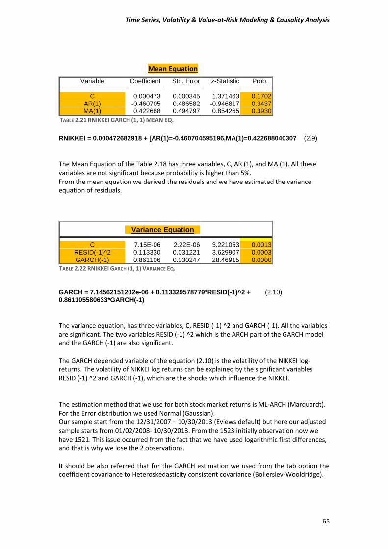
Time Series, Volatility & Value-at-Risk Modeling & Causality Analysis
65
Mean Equation
RNIKKEI = 0.000472682918 + [AR(1)=-0.460704595196,MA(1)=0.422688040307 (2.9)
The Mean Equation of the Table 2.18 has three variables, C, AR (1), and MA (1). All these variables are not significant because probability is higher than 5%. From the mean equation we derived the residuals and we have estimated the variance equation of residuals.
GARCH = 7.14562151202e-06 + 0.113329578779*RESID(-1)^2 + (2.10) 0.861105580633*GARCH(-1) The variance equation, has three variables, C, RESID (-1) ^2 and GARCH (-1). All the variables are significant. The two variables RESID (-1) ^2 which is the ARCH part of the GARCH model and the GARCH (-1) are also significant. The GARCH depended variable of the equation (2.10) is the volatility of the NIKKEI log-returns. The volatility of NIKKEI log returns can be explained by the significant variables RESID (-1) ^2 and GARCH (-1), which are the shocks which influence the NIKKEI. The estimation method that we use for both stock market returns is ML-ARCH (Marquardt). For the Error distribution we used Normal (Gaussian). Our sample start from the 12/31/2007 – 10/30/2013 (Eviews default) but here our adjusted sample starts from 01/02/2008- 10/30/2013. From the 1523 initially observation now we have 1521. This issue occurred from the fact that we have used logarithmic first differences, and that is why we lose the 2 observations. It should be also referred that for the GARCH estimation we used from the tab option the coefficient covariance to Heteroskedasticity consistent covariance (Bollerslev-Wooldridge).
Variable Coefficient Std. Error z-Statistic Prob. C 0.000473 0.000345 1.371463 0.1702
AR(1) -0.460705 0.486582 -0.946817 0.3437 MA(1) 0.422688 0.494797 0.854265 0.3930
TABLE 2.21 RNIKKEI GARCH (1, 1) MEAN EQ.
Variance Equation C 7.15E-06 2.22E-06 3.221053 0.0013
RESID(-1)^2 0.113330 0.031221 3.629907 0.0003 GARCH(-1) 0.861106 0.030247 28.46915 0.0000
TABLE 2.22 RNIKKEI GARCH (1, 1) VARIANCE EQ.
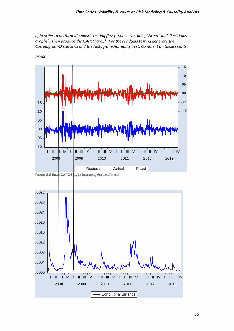
Time Series, Volatility & Value-at-Risk Modeling & Causality Analysis
66
c) In order to perform diagnostic testing first produce “Actual”, “Fitted” and “Residuals graphs”. Then produce the GARCH graph. For the residuals testing generate the Correlogram-Q statistics and the Histogram-Normality Test. Comment on these results. RDAX
FIGURE 2.8 RDAX GARCH (1, 1) RESIDUAL, ACTUAL, FITTED
-.10
-.05
.00
.05
.10
.15
-.10
-.05
.00
.05
.10
.15
I II III IV I II III IV I II III IV I II III IV I II III IV I II III IV
2008 2009 2010 2011 2012 2013
Residual Actual Fitted
.0000
.0004
.0008
.0012
.0016
.0020
.0024
.0028
.0032
I II III IV I II III IV I II III IV I II III IV I II III IV I II III IV
2008 2009 2010 2011 2012 2013
Conditional variance
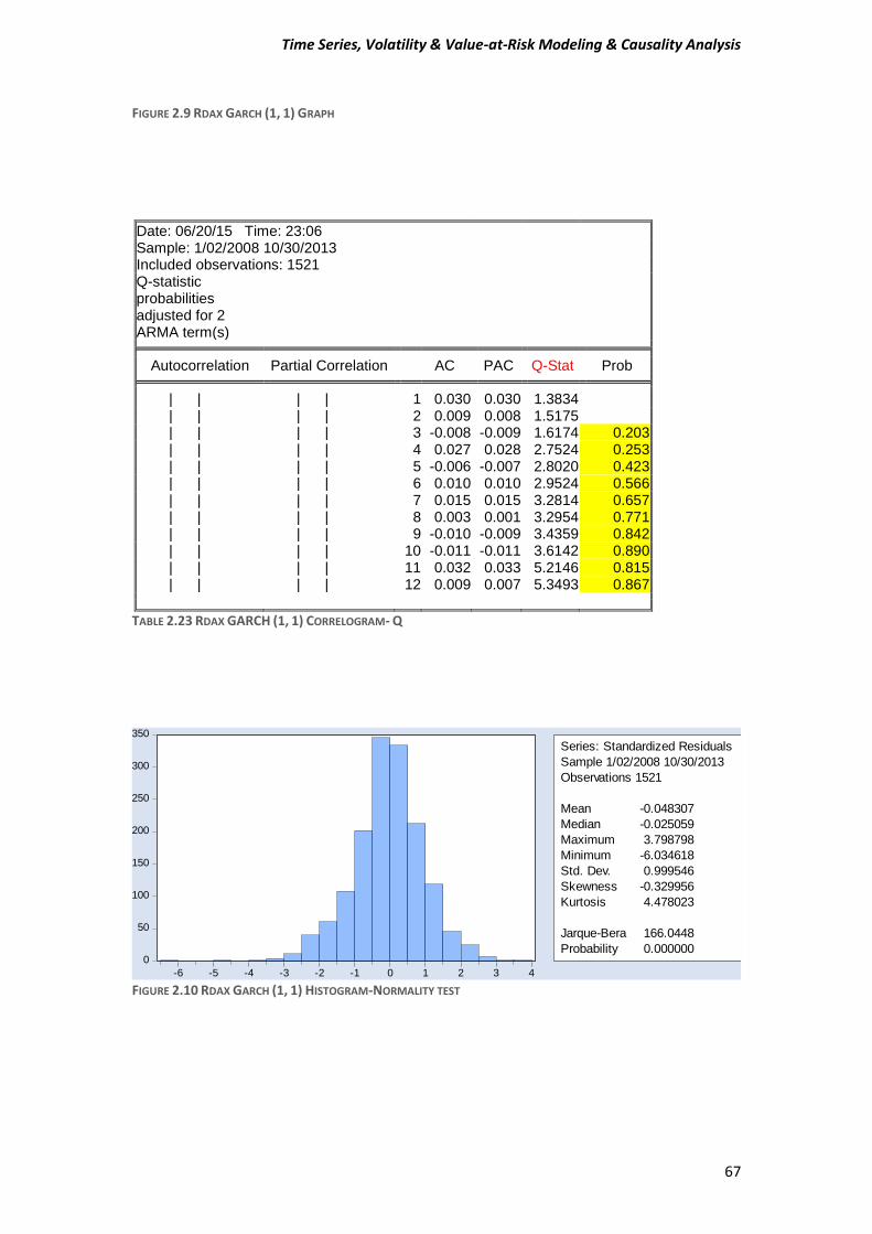
Time Series, Volatility & Value-at-Risk Modeling & Causality Analysis
67
FIGURE 2.9 RDAX GARCH (1, 1) GRAPH
Date: 06/20/15 Time: 23:06 Sample: 1/02/2008 10/30/2013 Included observations: 1521 Q-statistic probabilities adjusted for 2 ARMA term(s)
Autocorrelation Partial Correlation AC PAC Q-Stat Prob | | | | 1 0.030 0.030 1.3834
| | | | 2 0.009 0.008 1.5175 | | | | 3 -0.008 -0.009 1.6174 0.203 | | | | 4 0.027 0.028 2.7524 0.253 | | | | 5 -0.006 -0.007 2.8020 0.423 | | | | 6 0.010 0.010 2.9524 0.566 | | | | 7 0.015 0.015 3.2814 0.657 | | | | 8 0.003 0.001 3.2954 0.771 | | | | 9 -0.010 -0.009 3.4359 0.842 | | | | 10 -0.011 -0.011 3.6142 0.890 | | | | 11 0.032 0.033 5.2146 0.815 | | | | 12 0.009 0.007 5.3493 0.867
TABLE 2.23 RDAX GARCH (1, 1) CORRELOGRAM- Q
FIGURE 2.10 RDAX GARCH (1, 1) HISTOGRAM-NORMALITY TEST
0
50
100
150
200
250
300
350
-6 -5 -4 -3 -2 -1 0 1 2 3 4
Series: Standardized Residuals
Sample 1/02/2008 10/30/2013
Observations 1521
Mean -0.048307
Median -0.025059
Maximum 3.798798
Minimum -6.034618
Std. Dev. 0.999546
Skewness -0.329956
Kurtosis 4.478023
Jarque-Bera 166.0448
Probability 0.000000
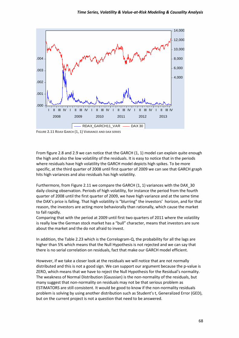
Time Series, Volatility & Value-at-Risk Modeling & Causality Analysis
68
FIGURE 2.11 RDAX GARCH (1, 1) VARIANCE AND DAX SERIES
From figure 2.8 and 2.9 we can notice that the GARCH (1, 1) model can explain quite enough the high and also the low volatility of the residuals. It is easy to notice that in the periods where residuals have high volatility the GARCH model depicts high spikes. To be more specific, at the third quarter of 2008 until first quarter of 2009 we can see that GARCH graph hits high variances and also residuals has high volatility. Furthermore, from Figure 2.11 we compare the GARCH (1, 1) variances with the DAX_30 daily closing observation. Periods of high volatility, for instance the period from the fourth quarter of 2008 until the first quarter of 2009, we have high variance and at the same time the DAX’s price is falling. That high volatility is “blurring” the investors’ horizon, and for that reason, the investors are acting more behaviorally than rationally, which cause the market to fall rapidly. Comparing that with the period at 2009 until first two quarters of 2011 where the volatility is really low the German stock market has a “bull” character, means that investors are sure about the market and the do not afraid to invest. In addition, the Table 2.23 which is the Correlogram-Q, the probability for all the lags are higher than 5% which means that the Null Hypothesis is not rejected and we can say that there is no serial correlation on residuals, fact that make our GARCH model efficient. However, if we take a closer look at the residuals we will notice that are not normally distributed and this is not a good sign. We can support our argument because the p-value is ZERO, which means that we have to reject the Null Hypothesis for the Residual’s normality. The weakness of Normal Distribution (Gaussian) is the non-normality of the residuals, but many suggest that non-normality on residuals may not be that serious problem as ESTIMATORS are still consistent. It would be good to know if the non-normality residuals problem is solving by using another distribution such as Student’s t, Generalized Error (GED), but on the current project is not a question that need to be answered.
.000
.001
.002
.003
.004
4,000
6,000
8,000
10,000
12,000
14,000
I II III IV I II III IV I II III IV I II III IV I II III IV I II III IV
2008 2009 2010 2011 2012 2013
RDAX_GARCH11_VAR DAX 30
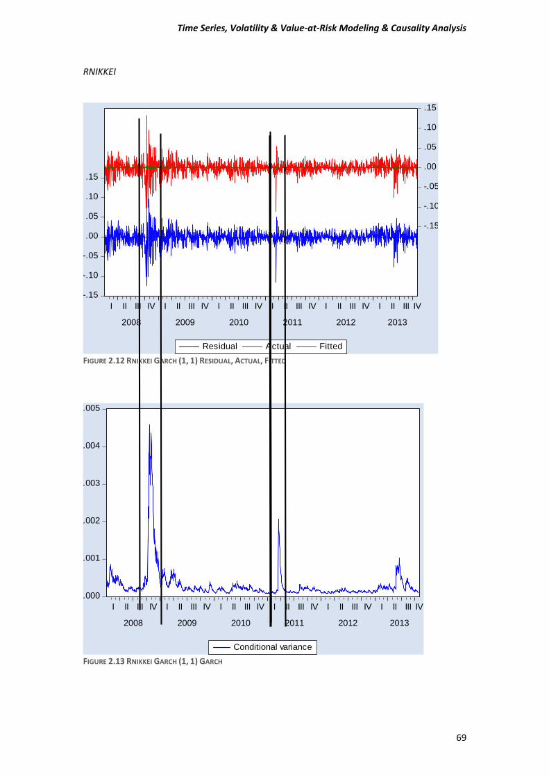
Time Series, Volatility & Value-at-Risk Modeling & Causality Analysis
69
RNIKKEI
FIGURE 2.12 RNIKKEI GARCH (1, 1) RESIDUAL, ACTUAL, FITTED
FIGURE 2.13 RNIKKEI GARCH (1, 1) GARCH
-.15
-.10
-.05
.00
.05
.10
.15
-.15
-.10
-.05
.00
.05
.10
.15
I II III IV I II III IV I II III IV I II III IV I II III IV I II III IV
2008 2009 2010 2011 2012 2013
Residual Actual Fitted
.000
.001
.002
.003
.004
.005
I II III IV I II III IV I II III IV I II III IV I II III IV I II III IV
2008 2009 2010 2011 2012 2013
Conditional variance
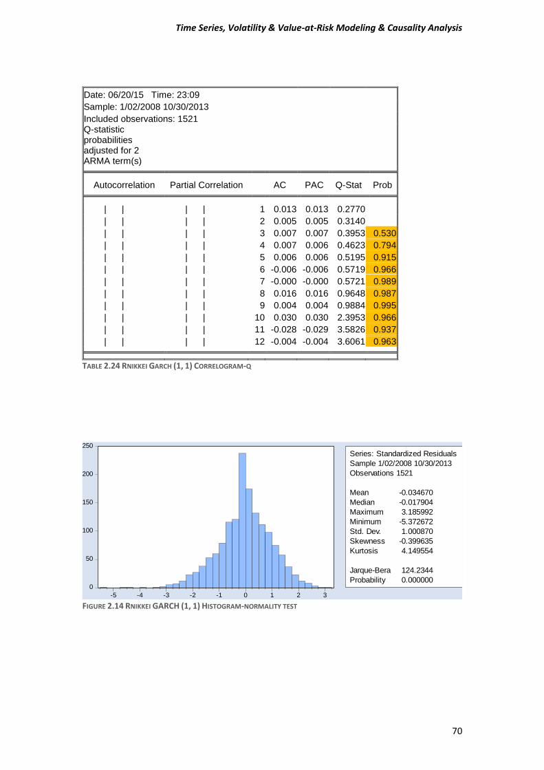
Time Series, Volatility & Value-at-Risk Modeling & Causality Analysis
70
FIGURE 2.14 RNIKKEI GARCH (1, 1) HISTOGRAM-NORMALITY TEST
0
50
100
150
200
250
-5 -4 -3 -2 -1 0 1 2 3
Series: Standardized Residuals
Sample 1/02/2008 10/30/2013
Observations 1521
Mean -0.034670
Median -0.017904
Maximum 3.185992
Minimum -5.372672
Std. Dev. 1.000870
Skewness -0.399635
Kurtosis 4.149554
Jarque-Bera 124.2344
Probability 0.000000
Date: 06/20/15 Time: 23:09
Sample: 1/02/2008 10/30/2013
Included observations: 1521 Q-statistic probabilities adjusted for 2 ARMA term(s)
Autocorrelation Partial Correlation AC PAC Q-Stat Prob
| | | | 1 0.013 0.013 0.2770
| | | | 2 0.005 0.005 0.3140
| | | | 3 0.007 0.007 0.3953 0.530
| | | | 4 0.007 0.006 0.4623 0.794
| | | | 5 0.006 0.006 0.5195 0.915
| | | | 6 -0.006 -0.006 0.5719 0.966
| | | | 7 -0.000 -0.000 0.5721 0.989
| | | | 8 0.016 0.016 0.9648 0.987
| | | | 9 0.004 0.004 0.9884 0.995
| | | | 10 0.030 0.030 2.3953 0.966
| | | | 11 -0.028 -0.029 3.5826 0.937
| | | | 12 -0.004 -0.004 3.6061 0.963
TABLE 2.24 RNIKKEI GARCH (1, 1) CORRELOGRAM-Q
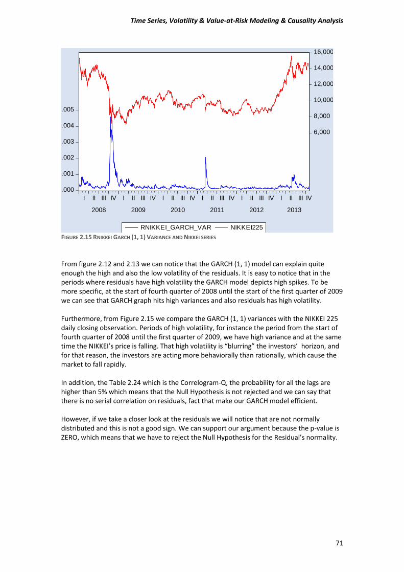
Time Series, Volatility & Value-at-Risk Modeling & Causality Analysis
71
FIGURE 2.15 RNIKKEI GARCH (1, 1) VARIANCE AND NIKKEI SERIES
From figure 2.12 and 2.13 we can notice that the GARCH (1, 1) model can explain quite enough the high and also the low volatility of the residuals. It is easy to notice that in the periods where residuals have high volatility the GARCH model depicts high spikes. To be more specific, at the start of fourth quarter of 2008 until the start of the first quarter of 2009 we can see that GARCH graph hits high variances and also residuals has high volatility. Furthermore, from Figure 2.15 we compare the GARCH (1, 1) variances with the NIKKEI 225 daily closing observation. Periods of high volatility, for instance the period from the start of fourth quarter of 2008 until the first quarter of 2009, we have high variance and at the same time the NIKKEI’s price is falling. That high volatility is “blurring” the investors’ horizon, and for that reason, the investors are acting more behaviorally than rationally, which cause the market to fall rapidly. In addition, the Table 2.24 which is the Correlogram-Q, the probability for all the lags are higher than 5% which means that the Null Hypothesis is not rejected and we can say that there is no serial correlation on residuals, fact that make our GARCH model efficient. However, if we take a closer look at the residuals we will notice that are not normally distributed and this is not a good sign. We can support our argument because the p-value is ZERO, which means that we have to reject the Null Hypothesis for the Residual’s normality.
.000
.001
.002
.003
.004
.005
6,000
8,000
10,000
12,000
14,000
16,000
I II III IV I II III IV I II III IV I II III IV I II III IV I II III IV
2008 2009 2010 2011 2012 2013
RNIKKEI_GARCH_VAR NIKKEI225
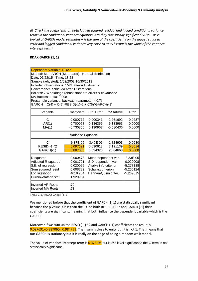
Time Series, Volatility & Value-at-Risk Modeling & Causality Analysis
72
d) Check the coefficients on both lagged squared residual and lagged conditional variance terms in the conditional variance equation. Are they statistically significant? Also – as is typical of GARCH model estimates – is the sum of the coefficients on the lagged squared error and lagged conditional variance very close to unity? What is the value of the variance intercept term? RDAX GARCH (1, 1) Dependent Variable: RDAX Method: ML - ARCH (Marquardt) - Normal distribution Date: 06/22/15 Time: 18:28 Sample (adjusted): 1/02/2008 10/30/2013 Included observations: 1521 after adjustments Convergence achieved after 17 iterations Bollerslev-Wooldridge robust standard errors & covariance MA Backcast: 1/01/2008 Presample variance: backcast (parameter = 0.7) GARCH = C(4) + C(5)*RESID(-1)^2 + C(6)*GARCH(-1)
Variable Coefficient Std. Error z-Statistic Prob. C 0.000772 0.000341 2.261692 0.0237
AR(1) 0.700098 0.136366 5.133963 0.0000 MA(1) -0.730855 0.130967 -5.580436 0.0000
Variance Equation C 6.37E-06 3.49E-06 1.824903 0.0680
RESID(-1)^2 0.097691 0.030613 3.191139 0.0014 GARCH(-1) 0.887060 0.034320 25.84668 0.0000
R-squared -0.000473 Mean dependent var 3.33E-05
Adjusted R-squared -0.001791 S.D. dependent var 0.020008 S.E. of regression 0.020026 Akaike info criterion -5.277138 Sum squared resid 0.608782 Schwarz criterion -5.256124 Log likelihood 4019.264 Hannan-Quinn criter. -5.269315 Durbin-Watson stat 1.929954
Inverted AR Roots .70
Inverted MA Roots .73
TABLE 2.17 RDAX GARCH (1, 1)
We mentioned before that the coefficient of GARCH (1, 1) are statistically significant because the p-value is less than the 5% so both RESID (-1) ^2 and GARCH (-1) their coefficients are significant, meaning that both influence the dependent variable which is the GARCH. Moreover if we sum up the RESID (-1) ^2 and GARCH (-1) coefficients the result is 0.097691+0.887060= 0.984751. Their sum is close to unity but it is not 1. That means that our GARCH is stationary but it is really on the edge of being a random walk model. The value of variance intercept term is 6.37E-06 but is 5% level significance the C term is not
statistically significant.
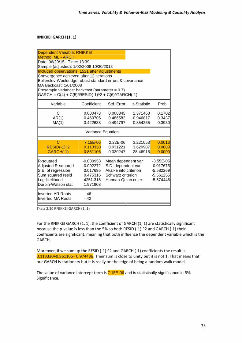
Time Series, Volatility & Value-at-Risk Modeling & Causality Analysis
73
RNIKKEI GARCH (1, 1)
Dependent Variable: RNIKKEI Method: ML - ARCH Date: 06/20/15 Time: 18:39 Sample (adjusted): 1/02/2008 10/30/2013 Included observations: 1521 after adjustments Convergence achieved after 12 iterations Bollerslev-Wooldridge robust standard errors & covariance MA Backcast: 1/01/2008 Presample variance: backcast (parameter = 0.7) GARCH = C(4) + C(5)*RESID(-1)^2 + C(6)*GARCH(-1)
Variable Coefficient Std. Error z-Statistic Prob. C 0.000473 0.000345 1.371463 0.1702
AR(1) -0.460705 0.486582 -0.946817 0.3437 MA(1) 0.422688 0.494797 0.854265 0.3930
Variance Equation
C 7.15E-06 2.22E-06 3.221053 0.0013 RESID(-1)^2 0.113330 0.031221 3.629907 0.0003 GARCH(-1) 0.861106 0.030247 28.46915 0.0000
R-squared -0.000953 Mean dependent var -3.55E-05
Adjusted R-squared -0.002272 S.D. dependent var 0.017675 S.E. of regression 0.017695 Akaike info criterion -5.582269 Sum squared resid 0.475316 Schwarz criterion -5.561255 Log likelihood 4251.316 Hannan-Quinn criter. -5.574446 Durbin-Watson stat 1.971908
Inverted AR Roots -.46
Inverted MA Roots -.42
TABLE 2.20 RNIKKEI GARCH (1, 1)
For the RNIKKEI GARCH (1, 1), the coefficient of GARCH (1, 1) are statistically significant because the p-value is less than the 5% so both RESID (-1) ^2 and GARCH (-1) their coefficients are significant, meaning that both influence the dependent variable which is the GARCH. Moreover, if we sum up the RESID (-1) ^2 and GARCH (-1) coefficients the result is 0.113330+0.861106= 0.974436. Their sum is close to unity but it is not 1. That means that our GARCH is stationary but it is really on the edge of being a random walk model. The value of variance intercept term is 7.15E-06 and is statistically significance in 5% Significance.
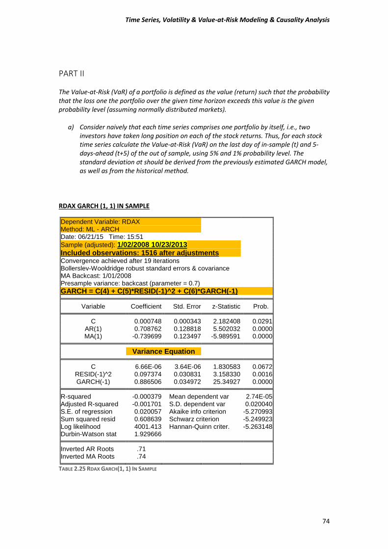
Time Series, Volatility & Value-at-Risk Modeling & Causality Analysis
74
PART II The Value-at-Risk (VaR) of a portfolio is defined as the value (return) such that the probability that the loss one the portfolio over the given time horizon exceeds this value is the given probability level (assuming normally distributed markets).
a) Consider naively that each time series comprises one portfolio by itself, i.e., two investors have taken long position on each of the stock returns. Thus, for each stock time series calculate the Value-at-Risk (VaR) on the last day of in-sample (t) and 5-days-ahead (t+5) of the out of sample, using 5% and 1% probability level. The standard deviation σt should be derived from the previously estimated GARCH model, as well as from the historical method.
RDAX GARCH (1, 1) IN SAMPLE
Dependent Variable: RDAX Method: ML - ARCH Date: 06/21/15 Time: 15:51
Sample (adjusted): 1/02/2008 10/23/2013
Included observations: 1516 after adjustments Convergence achieved after 19 iterations Bollerslev-Wooldridge robust standard errors & covariance MA Backcast: 1/01/2008 Presample variance: backcast (parameter = 0.7)
GARCH = C(4) + C(5)*RESID(-1)^2 + C(6)*GARCH(-1) Variable Coefficient Std. Error z-Statistic Prob. C 0.000748 0.000343 2.182408 0.0291
AR(1) 0.708762 0.128818 5.502032 0.0000 MA(1) -0.739699 0.123497 -5.989591 0.0000
Variance Equation C 6.66E-06 3.64E-06 1.830583 0.0672
RESID(-1)^2 0.097374 0.030831 3.158330 0.0016 GARCH(-1) 0.886506 0.034972 25.34927 0.0000
R-squared -0.000379 Mean dependent var 2.74E-05
Adjusted R-squared -0.001701 S.D. dependent var 0.020040 S.E. of regression 0.020057 Akaike info criterion -5.270993 Sum squared resid 0.608639 Schwarz criterion -5.249923 Log likelihood 4001.413 Hannan-Quinn criter. -5.263148 Durbin-Watson stat 1.929666
Inverted AR Roots .71
Inverted MA Roots .74
TABLE 2.25 RDAX GARCH(1, 1) IN SAMPLE
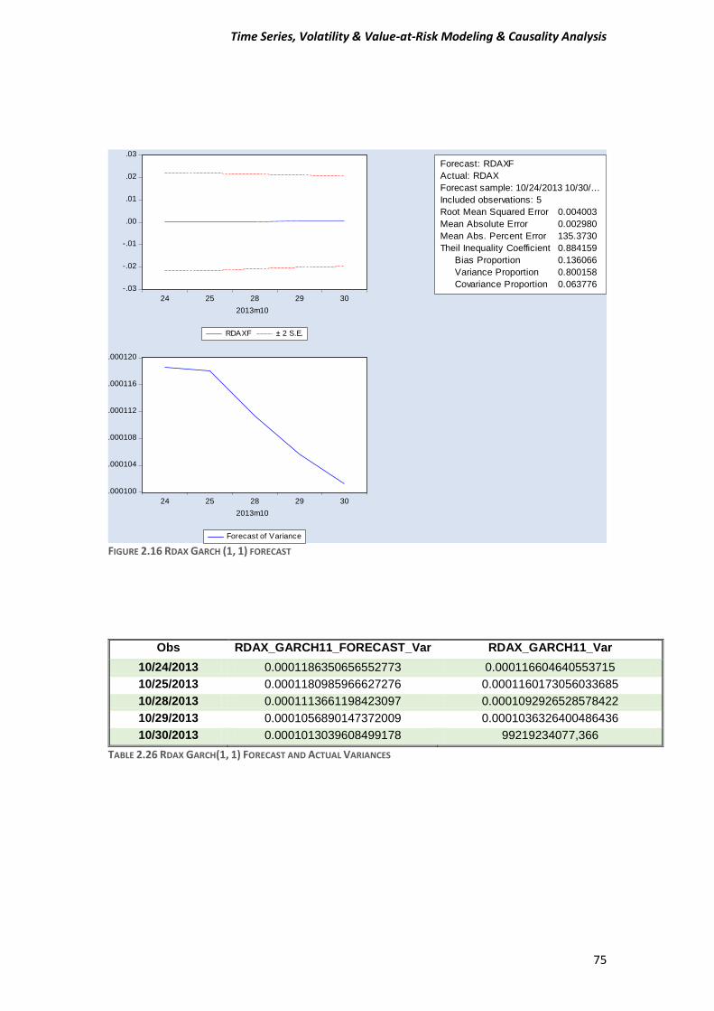
Time Series, Volatility & Value-at-Risk Modeling & Causality Analysis
75
FIGURE 2.16 RDAX GARCH (1, 1) FORECAST
Obs RDAX_GARCH11_FORECAST_Var RDAX_GARCH11_Var
10/24/2013 0.0001186350656552773 0.000116604640553715
10/25/2013 0.0001180985966627276 0.0001160173056033685
10/28/2013 0.0001113661198423097 0.0001092926528578422
10/29/2013 0.0001056890147372009 0.0001036326400486436
10/30/2013 0.0001013039608499178 99219234077,366
TABLE 2.26 RDAX GARCH(1, 1) FORECAST AND ACTUAL VARIANCES
-.03
-.02
-.01
.00
.01
.02
.03
24 25 28 29 30
2013m10
RDAXF ± 2 S.E.
Forecast: RDAXF
Actual: RDAX
Forecast sample: 10/24/2013 10/30/...
Included observations: 5
Root Mean Squared Error 0.004003
Mean Absolute Error 0.002980
Mean Abs. Percent Error 135.3730
Theil Inequality Coefficient 0.884159
Bias Proportion 0.136066
Variance Proportion 0.800158
Covariance Proportion 0.063776
.000100
.000104
.000108
.000112
.000116
.000120
24 25 28 29 30
2013m10
Forecast of Variance
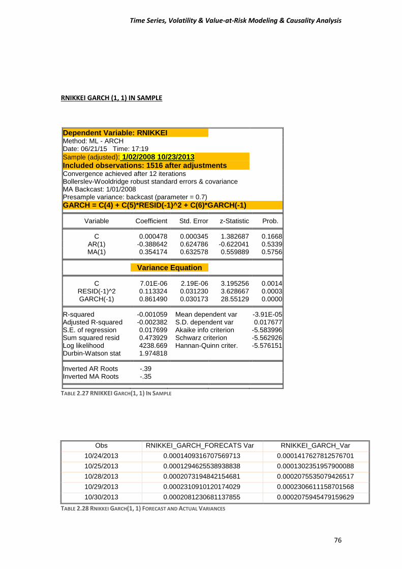
Time Series, Volatility & Value-at-Risk Modeling & Causality Analysis
76
RNIKKEI GARCH (1, 1) IN SAMPLE
Dependent Variable: RNIKKEI Method: ML - ARCH Date: 06/21/15 Time: 17:19
Sample (adjusted): 1/02/2008 10/23/2013
Included observations: 1516 after adjustments Convergence achieved after 12 iterations Bollerslev-Wooldridge robust standard errors & covariance MA Backcast: 1/01/2008 Presample variance: backcast (parameter = 0.7)
GARCH = C(4) + C(5)*RESID(-1)^2 + C(6)*GARCH(-1) Variable Coefficient Std. Error z-Statistic Prob. C 0.000478 0.000345 1.382687 0.1668
AR(1) -0.388642 0.624786 -0.622041 0.5339 MA(1) 0.354174 0.632578 0.559889 0.5756
Variance Equation C 7.01E-06 2.19E-06 3.195256 0.0014
RESID(-1)^2 0.113324 0.031230 3.628667 0.0003 GARCH(-1) 0.861490 0.030173 28.55129 0.0000
R-squared -0.001059 Mean dependent var -3.91E-05
Adjusted R-squared -0.002382 S.D. dependent var 0.017677 S.E. of regression 0.017699 Akaike info criterion -5.583996 Sum squared resid 0.473929 Schwarz criterion -5.562926 Log likelihood 4238.669 Hannan-Quinn criter. -5.576151 Durbin-Watson stat 1.974818
Inverted AR Roots -.39
Inverted MA Roots -.35
TABLE 2.27 RNIKKEI GARCH(1, 1) IN SAMPLE
Obs RNIKKEI_GARCH_FORECATS Var RNIKKEI_GARCH_Var
10/24/2013 0.0001409316707569713 0.0001417627812576701
10/25/2013 0.0001294625538938838 0.0001302351957900088
10/28/2013 0.0002073194842154681 0.0002075535079426517
10/29/2013 0.0002310910120174029 0.0002306611158701568
10/30/2013 0.0002081230681137855 0.0002075945479159629
TABLE 2.28 RNIKKEI GARCH(1, 1) FORECAST AND ACTUAL VARIANCES
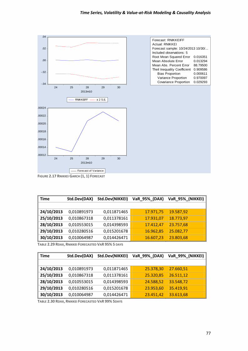
Time Series, Volatility & Value-at-Risk Modeling & Causality Analysis
77
FIGURE 2.17 RNIKKEI GARCH (1, 1) FORECAST
Time Std.Dev(DAX) Std.Dev(NIKKEI) VaR_95%_(DAX) VaR_95%_(NIKKEI)
24/10/2013 0,010891973 0,011871465 17.971,75 19.587,92
25/10/2013 0,010867318 0,011378161 17.931,07 18.773,97
28/10/2013 0,010553015 0,014398593 17.412,47 23.757,68
29/10/2013 0,010280516 0,015201678 16.962,85 25.082,77
30/10/2013 0,010064987 0,014426471 16.607,23 23.803,68
TABLE 2.29 RDAX, RNIKKEI FORECASTED VAR 95% 5 DAYS
Time Std.Dev(DAX) Std.Dev(NIKKEI) VaR_99%_(DAX) VaR_99%_(NIKKEI)
24/10/2013 0,010891973 0,011871465 25.378,30 27.660,51
25/10/2013 0,010867318 0,011378161 25.320,85 26.511,12
28/10/2013 0,010553015 0,014398593 24.588,52 33.548,72
29/10/2013 0,010280516 0,015201678 23.953,60 35.419,91
30/10/2013 0,010064987 0,014426471 23.451,42 33.613,68
TABLE 2.30 RDAX, RNIKKEI FORECASTED VAR 99% 5DAYS
-.04
-.02
.00
.02
.04
24 25 28 29 30
2013m10
RNIKKEIFF ± 2 S.E.
Forecast: RNIKKEIFF
Actual: RNIKKEI
Forecast sample: 10/24/2013 10/30/...
Included observations: 5
Root Mean Squared Error 0.016351
Mean Absolute Error 0.013294
Mean Abs. Percent Error 88.79500
Theil Inequality Coefficient 0.909586
Bias Proportion 0.000611
Variance Proportion 0.970097
Covariance Proportion 0.029293
.00012
.00014
.00016
.00018
.00020
.00022
.00024
24 25 28 29 30
2013m10
Forecast of Variance
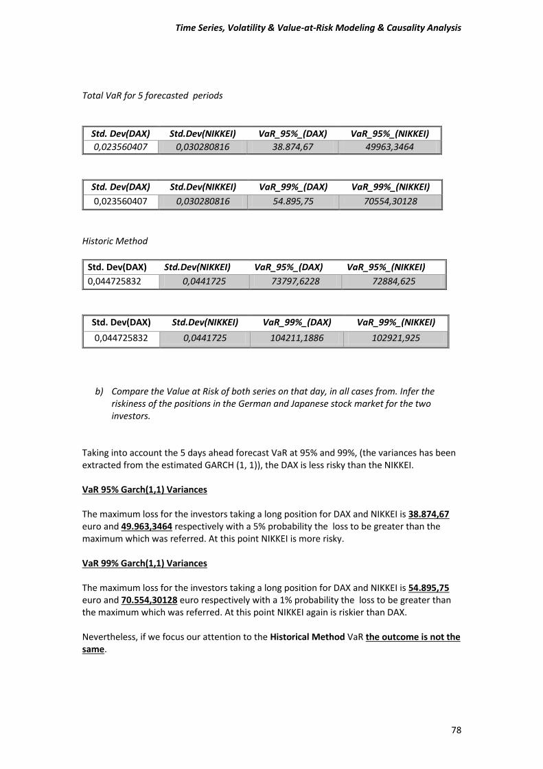
Time Series, Volatility & Value-at-Risk Modeling & Causality Analysis
78
Total VaR for 5 forecasted periods
Std. Dev(DAX) Std.Dev(NIKKEI) VaR_95%_(DAX) VaR_95%_(NIKKEI)
0,023560407 0,030280816 38.874,67 49963,3464
Std. Dev(DAX) Std.Dev(NIKKEI) VaR_99%_(DAX) VaR_99%_(NIKKEI)
0,023560407 0,030280816 54.895,75 70554,30128
Historic Method
Std. Dev(DAX) Std.Dev(NIKKEI) VaR_95%_(DAX) VaR_95%_(NIKKEI)
0,044725832 0,0441725 73797,6228 72884,625
Std. Dev(DAX) Std.Dev(NIKKEI) VaR_99%_(DAX) VaR_99%_(NIKKEI)
0,044725832 0,0441725 104211,1886 102921,925
b) Compare the Value at Risk of both series on that day, in all cases from. Infer the riskiness of the positions in the German and Japanese stock market for the two investors.
Taking into account the 5 days ahead forecast VaR at 95% and 99%, (the variances has been extracted from the estimated GARCH (1, 1)), the DAX is less risky than the NIKKEI. VaR 95% Garch(1,1) Variances The maximum loss for the investors taking a long position for DAX and NIKKEI is 38.874,67 euro and 49.963,3464 respectively with a 5% probability the loss to be greater than the maximum which was referred. At this point NIKKEI is more risky. VaR 99% Garch(1,1) Variances The maximum loss for the investors taking a long position for DAX and NIKKEI is 54.895,75 euro and 70.554,30128 euro respectively with a 1% probability the loss to be greater than the maximum which was referred. At this point NIKKEI again is riskier than DAX. Nevertheless, if we focus our attention to the Historical Method VaR the outcome is not the same.
Time Series, Volatility & Value-at-Risk Modeling & Causality Analysis
79
VaR 95% Historical Method Relying now on the historical method the DAX Value-at-Risk is 73.797,6228 euro when the NIKKEI’s Value-at-Risk is calculated at 72.884,625 less than the DAX. Meaning that there is a 5% the loss to be greater than the calculated VaR. In this particular situation DAX is riskier than the NIKKEI. But can we rely on this outcome? VaR 99% Historical Method Checking also the VaR at 99% significance level, NIKKEI’s VaR is still lower than the DAX’s because 102.921,25 is lower than 104.211,1886. In conclusion, if one of the investor chooses to invest based on the historical Method VaR and the other chooses with the GARCH (1,1) variances, one of the two will definitely loss a big portion of his portfolio value. And probably will be the first one because his analysis is based on an average variance when the other’s is based on a daily variance fluctuations. The variance is not standard, but it is changing through the time so we must take into consideration the variance’s changes in order to predict and to invest without having any loss.
*The VaR calculation = 𝑉𝑎𝑅 = 𝑎𝜎𝑊𝑜 a = the significance level 1% = 2,33 and 5% = 1,65. σ = standard deviation Wo= portfolio value, here we assuming a portfolio 1.000.000. euro
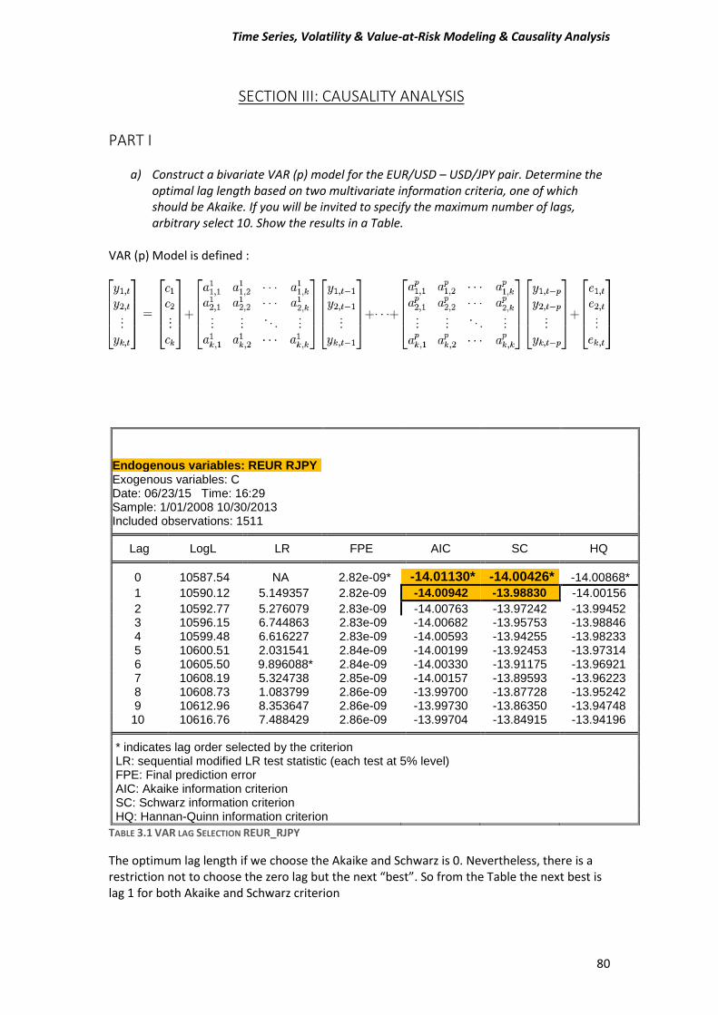
Time Series, Volatility & Value-at-Risk Modeling & Causality Analysis
80
SECTION III: CAUSALITY ANALYSIS
PART I
a) Construct a bivariate VAR (p) model for the EUR/USD – USD/JPY pair. Determine the optimal lag length based on two multivariate information criteria, one of which should be Akaike. If you will be invited to specify the maximum number of lags, arbitrary select 10. Show the results in a Table.
VAR (p) Model is defined :
Endogenous variables: REUR RJPY Exogenous variables: C Date: 06/23/15 Time: 16:29 Sample: 1/01/2008 10/30/2013 Included observations: 1511
Lag LogL LR FPE AIC SC HQ 0 10587.54 NA 2.82e-09* -14.01130* -14.00426* -14.00868*
1 10590.12 5.149357 2.82e-09 -14.00942 -13.98830 -14.00156
2 10592.77 5.276079 2.83e-09 -14.00763 -13.97242 -13.99452 3 10596.15 6.744863 2.83e-09 -14.00682 -13.95753 -13.98846 4 10599.48 6.616227 2.83e-09 -14.00593 -13.94255 -13.98233 5 10600.51 2.031541 2.84e-09 -14.00199 -13.92453 -13.97314 6 10605.50 9.896088* 2.84e-09 -14.00330 -13.91175 -13.96921 7 10608.19 5.324738 2.85e-09 -14.00157 -13.89593 -13.96223 8 10608.73 1.083799 2.86e-09 -13.99700 -13.87728 -13.95242 9 10612.96 8.353647 2.86e-09 -13.99730 -13.86350 -13.94748 10 10616.76 7.488429 2.86e-09 -13.99704 -13.84915 -13.94196 * indicates lag order selected by the criterion
LR: sequential modified LR test statistic (each test at 5% level) FPE: Final prediction error AIC: Akaike information criterion SC: Schwarz information criterion HQ: Hannan-Quinn information criterion
TABLE 3.1 VAR LAG SELECTION REUR_RJPY
The optimum lag length if we choose the Akaike and Schwarz is 0. Nevertheless, there is a restriction not to choose the zero lag but the next “best”. So from the Table the next best is lag 1 for both Akaike and Schwarz criterion
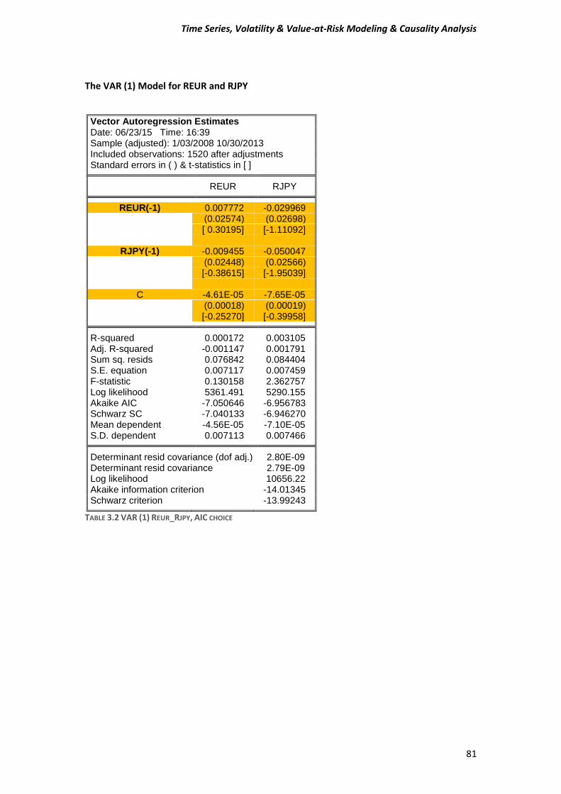
Time Series, Volatility & Value-at-Risk Modeling & Causality Analysis
81
The VAR (1) Model for REUR and RJPY
Vector Autoregression Estimates Date: 06/23/15 Time: 16:39 Sample (adjusted): 1/03/2008 10/30/2013 Included observations: 1520 after adjustments Standard errors in ( ) & t-statistics in [ ]
REUR RJPY REUR(-1) 0.007772 -0.029969 (0.02574) (0.02698) [ 0.30195] [-1.11092]
RJPY(-1) -0.009455 -0.050047 (0.02448) (0.02566) [-0.38615] [-1.95039]
C -4.61E-05 -7.65E-05 (0.00018) (0.00019) [-0.25270] [-0.39958] R-squared 0.000172 0.003105
Adj. R-squared -0.001147 0.001791 Sum sq. resids 0.076842 0.084404 S.E. equation 0.007117 0.007459 F-statistic 0.130158 2.362757 Log likelihood 5361.491 5290.155 Akaike AIC -7.050646 -6.956783 Schwarz SC -7.040133 -6.946270 Mean dependent -4.56E-05 -7.10E-05 S.D. dependent 0.007113 0.007466
Determinant resid covariance (dof adj.) 2.80E-09
Determinant resid covariance 2.79E-09 Log likelihood 10656.22 Akaike information criterion -14.01345 Schwarz criterion -13.99243
TABLE 3.2 VAR (1) REUR_RJPY, AIC CHOICE
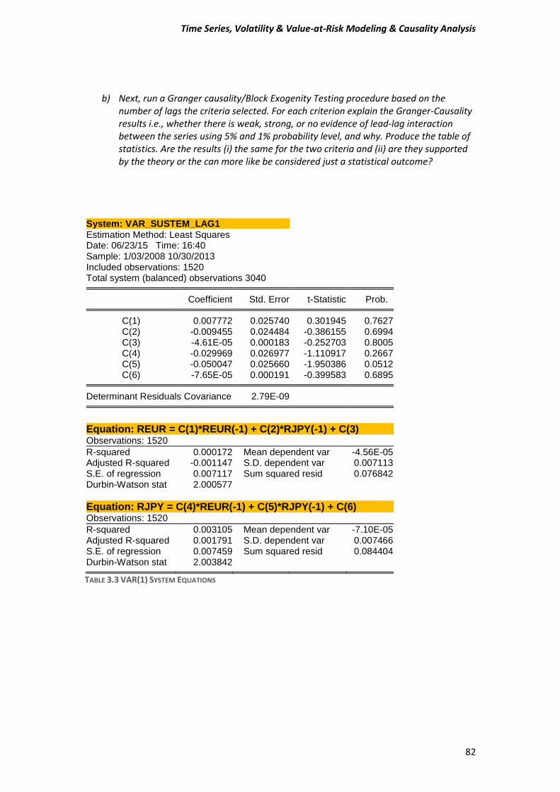
Time Series, Volatility & Value-at-Risk Modeling & Causality Analysis
82
b) Next, run a Granger causality/Block Exogenity Testing procedure based on the number of lags the criteria selected. For each criterion explain the Granger-Causality results i.e., whether there is weak, strong, or no evidence of lead-lag interaction between the series using 5% and 1% probability level, and why. Produce the table of statistics. Are the results (i) the same for the two criteria and (ii) are they supported by the theory or the can more like be considered just a statistical outcome?
System: VAR_SUSTEM_LAG1 Estimation Method: Least Squares Date: 06/23/15 Time: 16:40 Sample: 1/03/2008 10/30/2013 Included observations: 1520 Total system (balanced) observations 3040
Coefficient Std. Error t-Statistic Prob. C(1) 0.007772 0.025740 0.301945 0.7627
C(2) -0.009455 0.024484 -0.386155 0.6994 C(3) -4.61E-05 0.000183 -0.252703 0.8005 C(4) -0.029969 0.026977 -1.110917 0.2667 C(5) -0.050047 0.025660 -1.950386 0.0512 C(6) -7.65E-05 0.000191 -0.399583 0.6895
Determinant Residuals Covariance 2.79E-09
Equation: REUR = C(1)*REUR(-1) + C(2)*RJPY(-1) + C(3) Observations: 1520
R-squared 0.000172 Mean dependent var -4.56E-05 Adjusted R-squared -0.001147 S.D. dependent var 0.007113 S.E. of regression 0.007117 Sum squared resid 0.076842 Durbin-Watson stat 2.000577
Equation: RJPY = C(4)*REUR(-1) + C(5)*RJPY(-1) + C(6) Observations: 1520
R-squared 0.003105 Mean dependent var -7.10E-05 Adjusted R-squared 0.001791 S.D. dependent var 0.007466 S.E. of regression 0.007459 Sum squared resid 0.084404 Durbin-Watson stat 2.003842
TABLE 3.3 VAR(1) SYSTEM EQUATIONS
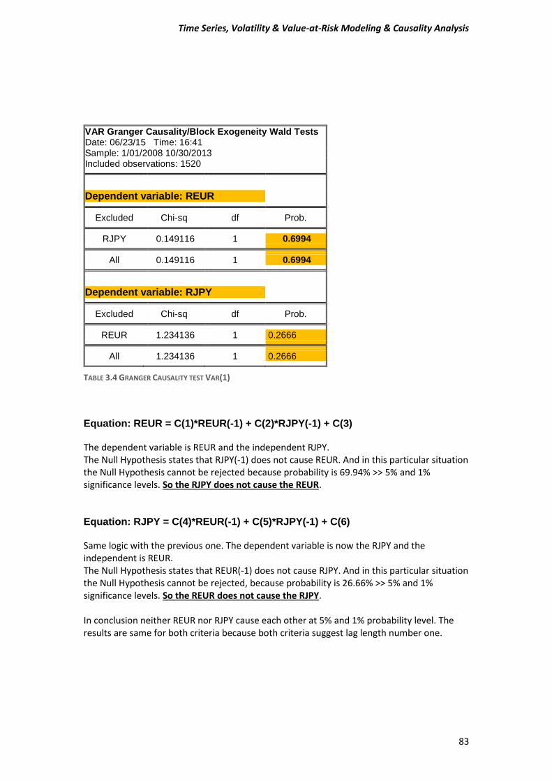
Time Series, Volatility & Value-at-Risk Modeling & Causality Analysis
83
TABLE 3.4 GRANGER CAUSALITY TEST VAR(1)
Equation: REUR = C(1)*REUR(-1) + C(2)*RJPY(-1) + C(3)
The dependent variable is REUR and the independent RJPY. The Null Hypothesis states that RJPY(-1) does not cause REUR. And in this particular situation the Null Hypothesis cannot be rejected because probability is 69.94% >> 5% and 1% significance levels. So the RJPY does not cause the REUR. Equation: RJPY = C(4)*REUR(-1) + C(5)*RJPY(-1) + C(6) Same logic with the previous one. The dependent variable is now the RJPY and the independent is REUR. The Null Hypothesis states that REUR(-1) does not cause RJPY. And in this particular situation the Null Hypothesis cannot be rejected, because probability is 26.66% >> 5% and 1% significance levels. So the REUR does not cause the RJPY. In conclusion neither REUR nor RJPY cause each other at 5% and 1% probability level. The results are same for both criteria because both criteria suggest lag length number one.
VAR Granger Causality/Block Exogeneity Wald Tests
Date: 06/23/15 Time: 16:41 Sample: 1/01/2008 10/30/2013 Included observations: 1520
Dependent variable: REUR Excluded Chi-sq df Prob. RJPY 0.149116 1 0.6994 All 0.149116 1 0.6994
Dependent variable: RJPY Excluded Chi-sq df Prob. REUR 1.234136 1 0.2666 All 1.234136 1 0.2666
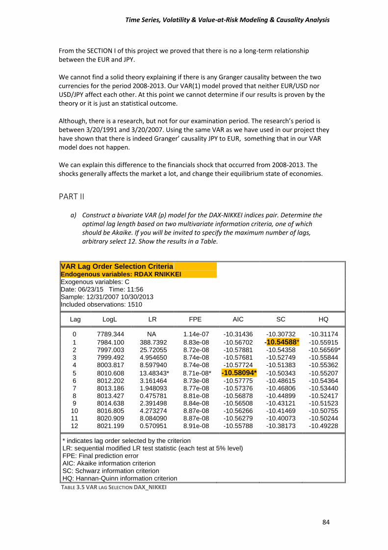
Time Series, Volatility & Value-at-Risk Modeling & Causality Analysis
84
From the SECTION I of this project we proved that there is no a long-term relationship between the EUR and JPY. We cannot find a solid theory explaining if there is any Granger causality between the two currencies for the period 2008-2013. Our VAR(1) model proved that neither EUR/USD nor USD/JPY affect each other. At this point we cannot determine if our results is proven by the theory or it is just an statistical outcome. Although, there is a research, but not for our examination period. The research’s period is between 3/20/1991 and 3/20/2007. Using the same VAR as we have used in our project they have shown that there is indeed Granger’ causality JPY to EUR, something that in our VAR model does not happen. We can explain this difference to the financials shock that occurred from 2008-2013. The shocks generally affects the market a lot, and change their equilibrium state of economies.
PART II
a) Construct a bivariate VAR (p) model for the DAX-NIKKEI indices pair. Determine the optimal lag length based on two multivariate information criteria, one of which should be Akaike. If you will be invited to specify the maximum number of lags, arbitrary select 12. Show the results in a Table.
VAR Lag Order Selection Criteria Endogenous variables: RDAX RNIKKEI Exogenous variables: C Date: 06/23/15 Time: 11:56 Sample: 12/31/2007 10/30/2013 Included observations: 1510
Lag LogL LR FPE AIC SC HQ 0 7789.344 NA 1.14e-07 -10.31436 -10.30732 -10.31174
1 7984.100 388.7392 8.83e-08 -10.56702 -10.54588* -10.55915 2 7997.003 25.72055 8.72e-08 -10.57881 -10.54358 -10.56569* 3 7999.492 4.954650 8.74e-08 -10.57681 -10.52749 -10.55844 4 8003.817 8.597940 8.74e-08 -10.57724 -10.51383 -10.55362
5 8010.608 13.48343* 8.71e-08* -10.58094* -10.50343 -10.55207 6 8012.202 3.161464 8.73e-08 -10.57775 -10.48615 -10.54364 7 8013.186 1.948093 8.77e-08 -10.57376 -10.46806 -10.53440 8 8013.427 0.475781 8.81e-08 -10.56878 -10.44899 -10.52417 9 8014.638 2.391498 8.84e-08 -10.56508 -10.43121 -10.51523 10 8016.805 4.273274 8.87e-08 -10.56266 -10.41469 -10.50755 11 8020.909 8.084090 8.87e-08 -10.56279 -10.40073 -10.50244 12 8021.199 0.570951 8.91e-08 -10.55788 -10.38173 -10.49228 * indicates lag order selected by the criterion
LR: sequential modified LR test statistic (each test at 5% level) FPE: Final prediction error AIC: Akaike information criterion SC: Schwarz information criterion HQ: Hannan-Quinn information criterion
TABLE 3.5 VAR LAG SELECTION DAX_NIKKEI
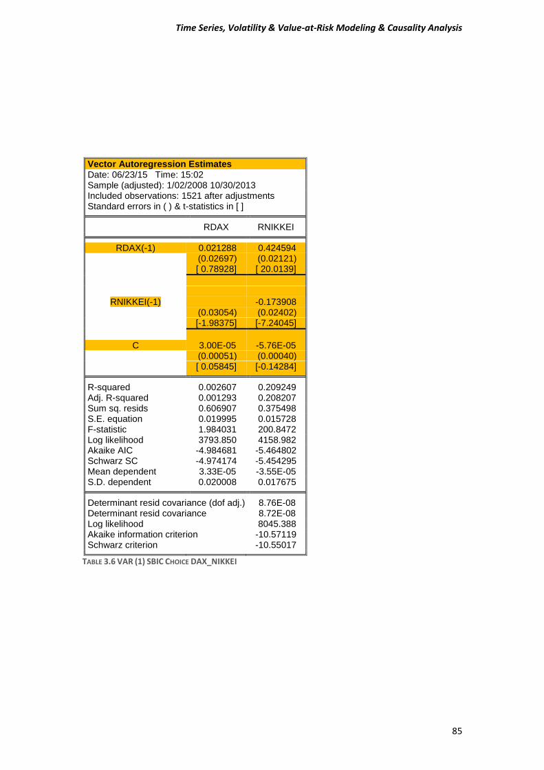
Time Series, Volatility & Value-at-Risk Modeling & Causality Analysis
85
Vector Autoregression Estimates Date: 06/23/15 Time: 15:02 Sample (adjusted): 1/02/2008 10/30/2013 Included observations: 1521 after adjustments Standard errors in ( ) & t-statistics in [ ]
RDAX RNIKKEI RDAX(-1) 0.021288 0.424594 (0.02697) (0.02121) [ 0.78928] [ 20.0139]
RNIKKEI(-1) -0.173908
(0.03054) (0.02402) [-1.98375] [-7.24045]
C 3.00E-05 -5.76E-05 (0.00051) (0.00040) [ 0.05845] [-0.14284] R-squared 0.002607 0.209249
Adj. R-squared 0.001293 0.208207 Sum sq. resids 0.606907 0.375498 S.E. equation 0.019995 0.015728 F-statistic 1.984031 200.8472 Log likelihood 3793.850 4158.982 Akaike AIC -4.984681 -5.464802 Schwarz SC -4.974174 -5.454295 Mean dependent 3.33E-05 -3.55E-05 S.D. dependent 0.020008 0.017675
Determinant resid covariance (dof adj.) 8.76E-08
Determinant resid covariance 8.72E-08 Log likelihood 8045.388 Akaike information criterion -10.57119 Schwarz criterion -10.55017
TABLE 3.6 VAR (1) SBIC CHOICE DAX_NIKKEI
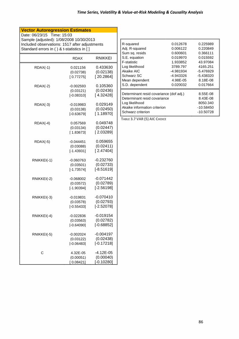
Time Series, Volatility & Value-at-Risk Modeling & Causality Analysis
86
TABLE 3.7 VAR (5) AIC CHOICE
Vector Autoregression Estimates
Date: 06/23/15 Time: 15:03 Sample (adjusted): 1/08/2008 10/30/2013 Included observations: 1517 after adjustments Standard errors in ( ) & t-statistics in [ ]
RDAX RNIKKEI RDAX(-1) 0.021156 0.433630
(0.02738) (0.02138)
[ 0.77275] [ 20.2864]
RDAX(-2) -0.002593 0.105360
(0.03121) (0.02436)
[-0.08310] [ 4.32428]
RDAX(-3) -0.019983 0.029149
(0.03138) (0.02450)
[-0.63679] [ 1.18970]
RDAX(-4) 0.057569 0.049748
(0.03134) (0.02447)
[ 1.83673] [ 2.03289]
RDAX(-5) -0.044451 0.059655
(0.03088) (0.02411)
[-1.43931] [ 2.47404]
RNIKKEI(-1) -0.060763 -0.232760
(0.03501) (0.02733)
[-1.73574] [-8.51619]
RNIKKEI(-2) -0.068002 -0.071442
(0.03572) (0.02789)
[-1.90394] [-2.56198]
RNIKKEI(-3) -0.019831 -0.070410
(0.03578) (0.02793)
[-0.55433] [-2.52078]
RNIKKEI(-4) -0.022836 -0.019154
(0.03563) (0.02782)
[-0.64090] [-0.68852]
RNIKKEI(-5) -0.002024 -0.004197
(0.03122) (0.02438)
[-0.06483] [-0.17218]
C 4.32E-05 -4.12E-05
(0.00051) (0.00040)
[ 0.08421] [-0.10280]
R-squared 0.012678 0.225989
Adj. R-squared 0.006122 0.220849
Sum sq. resids 0.600601 0.366111
S.E. equation 0.019970 0.015592
F-statistic 1.933852 43.97084
Log likelihood 3789.797 4165.251
Akaike AIC -4.981934 -5.476929
Schwarz SC -4.943326 -5.438320
Mean dependent 4.98E-05 8.18E-08
S.D. dependent 0.020032 0.017664 Determinant resid covariance (dof adj.) 8.55E-08
Determinant resid covariance 8.43E-08
Log likelihood 8050.340
Akaike information criterion -10.58450
Schwarz criterion -10.50728
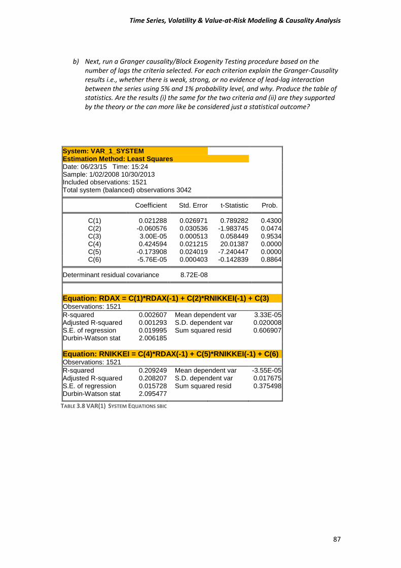
Time Series, Volatility & Value-at-Risk Modeling & Causality Analysis
87
b) Next, run a Granger causality/Block Exogenity Testing procedure based on the
number of lags the criteria selected. For each criterion explain the Granger-Causality results i.e., whether there is weak, strong, or no evidence of lead-lag interaction between the series using 5% and 1% probability level, and why. Produce the table of statistics. Are the results (i) the same for the two criteria and (ii) are they supported by the theory or the can more like be considered just a statistical outcome?
System: VAR_1_SYSTEM Estimation Method: Least Squares Date: 06/23/15 Time: 15:24 Sample: 1/02/2008 10/30/2013 Included observations: 1521 Total system (balanced) observations 3042
Coefficient Std. Error t-Statistic Prob. C(1) 0.021288 0.026971 0.789282 0.4300
C(2) -0.060576 0.030536 -1.983745 0.0474 C(3) 3.00E-05 0.000513 0.058449 0.9534 C(4) 0.424594 0.021215 20.01387 0.0000 C(5) -0.173908 0.024019 -7.240447 0.0000 C(6) -5.76E-05 0.000403 -0.142839 0.8864
Determinant residual covariance 8.72E-08
Equation: RDAX = C(1)*RDAX(-1) + C(2)*RNIKKEI(-1) + C(3) Observations: 1521
R-squared 0.002607 Mean dependent var 3.33E-05 Adjusted R-squared 0.001293 S.D. dependent var 0.020008 S.E. of regression 0.019995 Sum squared resid 0.606907 Durbin-Watson stat 2.006185
Equation: RNIKKEI = C(4)*RDAX(-1) + C(5)*RNIKKEI(-1) + C(6) Observations: 1521
R-squared 0.209249 Mean dependent var -3.55E-05 Adjusted R-squared 0.208207 S.D. dependent var 0.017675 S.E. of regression 0.015728 Sum squared resid 0.375498 Durbin-Watson stat 2.095477
TABLE 3.8 VAR(1) SYSTEM EQUATIONS SBIC
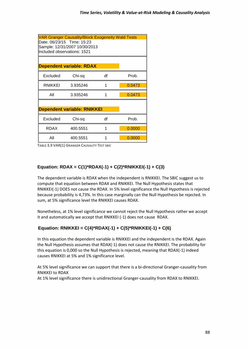
Time Series, Volatility & Value-at-Risk Modeling & Causality Analysis
88
VAR Granger Causality/Block Exogeneity Wald Tests Date: 06/23/15 Time: 15:23 Sample: 12/31/2007 10/30/2013 Included observations: 1521
Dependent variable: RDAX Excluded Chi-sq df Prob. RNIKKEI 3.935246 1 0.0473 All 3.935246 1 0.0473
Dependent variable: RNIKKEI Excluded Chi-sq df Prob. RDAX 400.5551 1 0.0000 All 400.5551 1 0.0000
TABLE 3.9 VAR(1) GRANGER CAUSALITY TEST SBIC
Equation: RDAX = C(1)*RDAX(-1) + C(2)*RNIKKEI(-1) + C(3) The dependent variable is RDAX when the independent is RNIKKEI. The SBIC suggest us to compute that equation between RDAX and RNIKKEI. The Null Hypothesis states that RNIKKEI(-1) DOES not cause the RDAX. In 5% level significance the Null Hypothesis is rejected because probability is 4,73%. In this case marginally can the Null Hypothesis be rejected. In sum, at 5% significance level the RNIKKEI causes RDAX. Nonetheless, at 1% level significance we cannot reject the Null Hypothesis rather we accept it and automatically we accept that RNIKKEI (-1) does not cause RDAX. Equation: RNIKKEI = C(4)*RDAX(-1) + C(5)*RNIKKEI(-1) + C(6) In this equation the dependent variable is RNIKKEI and the independent is the RDAX. Again the Null Hypothesis assumes that RDAX(-1) does not cause the RNIKKEI. The probability for this equation is 0,000 so the Null Hypothesis is rejected, meaning that RDAX(-1) indeed causes RNIKKEI at 5% and 1% significance level. At 5% level significance we can support that there is a bi-directional Granger-causality from RNIKKEI to RDAX At 1% level significance there is unidirectional Granger-causality from RDAX to RNIKKEI.
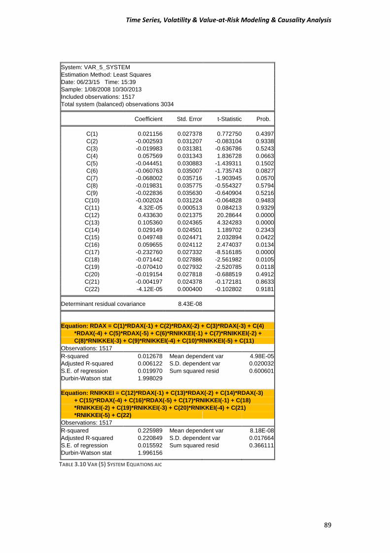
Time Series, Volatility & Value-at-Risk Modeling & Causality Analysis
89
System: VAR_5_SYSTEM
Estimation Method: Least Squares
Date: 06/23/15 Time: 15:39
Sample: 1/08/2008 10/30/2013
Included observations: 1517
Total system (balanced) observations 3034 Coefficient Std. Error t-Statistic Prob. C(1) 0.021156 0.027378 0.772750 0.4397
C(2) -0.002593 0.031207 -0.083104 0.9338
C(3) -0.019983 0.031381 -0.636786 0.5243
C(4) 0.057569 0.031343 1.836728 0.0663
C(5) -0.044451 0.030883 -1.439311 0.1502
C(6) -0.060763 0.035007 -1.735743 0.0827
C(7) -0.068002 0.035716 -1.903945 0.0570
C(8) -0.019831 0.035775 -0.554327 0.5794
C(9) -0.022836 0.035630 -0.640904 0.5216
C(10) -0.002024 0.031224 -0.064828 0.9483
C(11) 4.32E-05 0.000513 0.084213 0.9329
C(12) 0.433630 0.021375 20.28644 0.0000
C(13) 0.105360 0.024365 4.324283 0.0000
C(14) 0.029149 0.024501 1.189702 0.2343
C(15) 0.049748 0.024471 2.032894 0.0422
C(16) 0.059655 0.024112 2.474037 0.0134
C(17) -0.232760 0.027332 -8.516185 0.0000
C(18) -0.071442 0.027886 -2.561982 0.0105
C(19) -0.070410 0.027932 -2.520785 0.0118
C(20) -0.019154 0.027818 -0.688519 0.4912
C(21) -0.004197 0.024378 -0.172181 0.8633
C(22) -4.12E-05 0.000400 -0.102802 0.9181 Determinant residual covariance 8.43E-08
Equation: RDAX = C(1)*RDAX(-1) + C(2)*RDAX(-2) + C(3)*RDAX(-3) + C(4)
*RDAX(-4) + C(5)*RDAX(-5) + C(6)*RNIKKEI(-1) + C(7)*RNIKKEI(-2) +
C(8)*RNIKKEI(-3) + C(9)*RNIKKEI(-4) + C(10)*RNIKKEI(-5) + C(11)
Observations: 1517
R-squared 0.012678 Mean dependent var 4.98E-05
Adjusted R-squared 0.006122 S.D. dependent var 0.020032
S.E. of regression 0.019970 Sum squared resid 0.600601
Durbin-Watson stat 1.998029
Equation: RNIKKEI = C(12)*RDAX(-1) + C(13)*RDAX(-2) + C(14)*RDAX(-3)
+ C(15)*RDAX(-4) + C(16)*RDAX(-5) + C(17)*RNIKKEI(-1) + C(18)
*RNIKKEI(-2) + C(19)*RNIKKEI(-3) + C(20)*RNIKKEI(-4) + C(21)
*RNIKKEI(-5) + C(22)
Observations: 1517
R-squared 0.225989 Mean dependent var 8.18E-08
Adjusted R-squared 0.220849 S.D. dependent var 0.017664
S.E. of regression 0.015592 Sum squared resid 0.366111
Durbin-Watson stat 1.996156
TABLE 3.10 VAR (5) SYSTEM EQUATIONS AIC
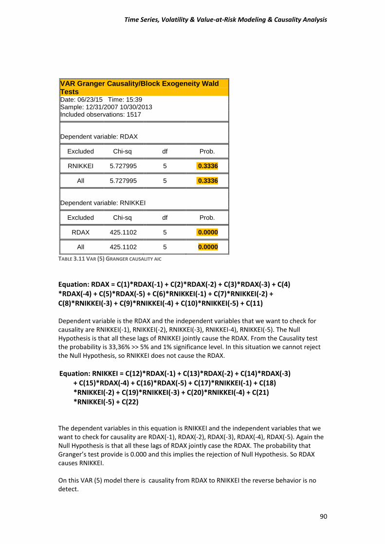
Time Series, Volatility & Value-at-Risk Modeling & Causality Analysis
90
VAR Granger Causality/Block Exogeneity Wald Tests
Date: 06/23/15 Time: 15:39 Sample: 12/31/2007 10/30/2013 Included observations: 1517
Dependent variable: RDAX Excluded Chi-sq df Prob. RNIKKEI 5.727995 5 0.3336 All 5.727995 5 0.3336
Dependent variable: RNIKKEI Excluded Chi-sq df Prob. RDAX 425.1102 5 0.0000 All 425.1102 5 0.0000
TABLE 3.11 VAR (5) GRANGER CAUSALITY AIC
Equation: RDAX = C(1)*RDAX(-1) + C(2)*RDAX(-2) + C(3)*RDAX(-3) + C(4) *RDAX(-4) + C(5)*RDAX(-5) + C(6)*RNIKKEI(-1) + C(7)*RNIKKEI(-2) + C(8)*RNIKKEI(-3) + C(9)*RNIKKEI(-4) + C(10)*RNIKKEI(-5) + C(11) Dependent variable is the RDAX and the independent variables that we want to check for causality are RNIKKEI(-1), RNIKKEI(-2), RNIKKEI(-3), RNIKKEI-4), RNIKKEI(-5). The Null Hypothesis is that all these lags of RNIKKEI jointly cause the RDAX. From the Causality test the probability is 33,36% >> 5% and 1% significance level. In this situation we cannot reject the Null Hypothesis, so RNIKKEI does not cause the RDAX.
Equation: RNIKKEI = C(12)*RDAX(-1) + C(13)*RDAX(-2) + C(14)*RDAX(-3) + C(15)*RDAX(-4) + C(16)*RDAX(-5) + C(17)*RNIKKEI(-1) + C(18) *RNIKKEI(-2) + C(19)*RNIKKEI(-3) + C(20)*RNIKKEI(-4) + C(21) *RNIKKEI(-5) + C(22) The dependent variables in this equation is RNIKKEI and the independent variables that we want to check for causality are RDAX(-1), RDAX(-2), RDAX(-3), RDAX(-4), RDAX(-5). Again the Null Hypothesis is that all these lags of RDAX jointly case the RDAX. The probability that Granger’s test provide is 0.000 and this implies the rejection of Null Hypothesis. So RDAX causes RNIKKEI. On this VAR (5) model there is causality from RDAX to RNIKKEI the reverse behavior is no detect.
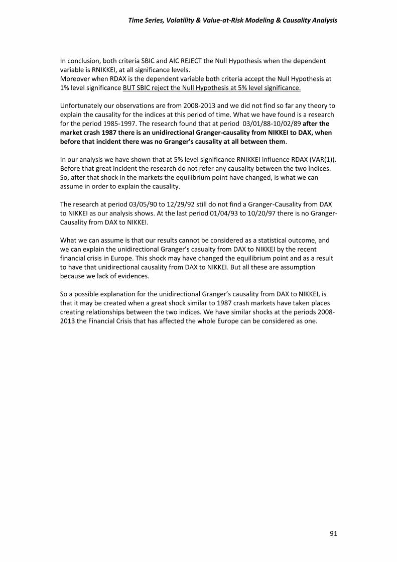
Time Series, Volatility & Value-at-Risk Modeling & Causality Analysis
91
In conclusion, both criteria SBIC and AIC REJECT the Null Hypothesis when the dependent variable is RNIKKEI, at all significance levels. Moreover when RDAX is the dependent variable both criteria accept the Null Hypothesis at 1% level significance BUT SBIC reject the Null Hypothesis at 5% level significance. Unfortunately our observations are from 2008-2013 and we did not find so far any theory to explain the causality for the indices at this period of time. What we have found is a research for the period 1985-1997. The research found that at period 03/01/88-10/02/89 after the market crash 1987 there is an unidirectional Granger-causality from NIKKEI to DAX, when before that incident there was no Granger’s causality at all between them. In our analysis we have shown that at 5% level significance RNIKKEI influence RDAX (VAR(1)). Before that great incident the research do not refer any causality between the two indices. So, after that shock in the markets the equilibrium point have changed, is what we can assume in order to explain the causality. The research at period 03/05/90 to 12/29/92 still do not find a Granger-Causality from DAX to NIKKEI as our analysis shows. At the last period 01/04/93 to 10/20/97 there is no Granger-Causality from DAX to NIKKEI. What we can assume is that our results cannot be considered as a statistical outcome, and we can explain the unidirectional Granger’s casualty from DAX to NIKKEI by the recent financial crisis in Europe. This shock may have changed the equilibrium point and as a result to have that unidirectional causality from DAX to NIKKEI. But all these are assumption because we lack of evidences. So a possible explanation for the unidirectional Granger’s causality from DAX to NIKKEI, is that it may be created when a great shock similar to 1987 crash markets have taken places creating relationships between the two indices. We have similar shocks at the periods 2008-2013 the Financial Crisis that has affected the whole Europe can be considered as one.

Time Series, Volatility & Value-at-Risk Modeling & Causality Analysis
92
REFERENCES ARIMASel (2010) http://www.eviews.com/Addins/addins.shtml Γ.Κ. Χρήστου (2007), Εισαγωγή στην Οικονομετρία, Τόμος Α’ & Β’, Gutenberg. Fabozzi Frank J., Focardi Sergio M., Jasic Teo, Mittnik Stefan, Rachiev Svetlozar T (2007)., “Financial Econometrics” From Basics to Advanced Modeling Techniques, Wiley Finance. Moslem Peymany(2009), A simple Eviews Program for ARMA selection, http://papers.ssrn.com/sol3/papers.cfm?abstract_id=1523045 Robert Dornau, Shock Around the Clock- On the Causal Relations Between International Stock Markets, the Strength of Causality and the Intensity of Shock Transmission. An Econometric Analysis. http://ftp.zew.de/pub/zew-docs/dp/dp1398.pdf Stelios D. Bekiros, Cees G.H. Diks (2008), The nonlinear dynamic relationship of exchange
rates: Parametric and nonparametric causality tests, doi:10.1016/j.jmacro.2008.04.001,
Journal of Macroeconomics. Yang Fan (2011), Are international stock market correlated? Comparing NIKKEI, Dow Jones, and DAX in the periods of 1991-2000 and 2001-2010, Jonkoping International Business School. Yoshihiro Kitamura (2012), Informational linkages among the major currencies in the EBS market: Evidence from the spot rates of the Euro, Yen and Swiss franc, pp (17-26),
doi:10.1016/j.japwor.2011.12.003, Japan and World Economy.
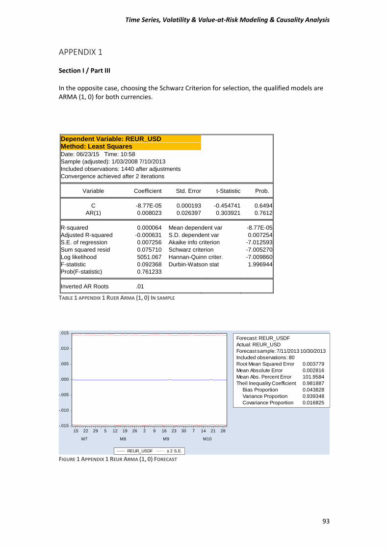
Time Series, Volatility & Value-at-Risk Modeling & Causality Analysis
93
APPENDIX 1 Section I / Part III In the opposite case, choosing the Schwarz Criterion for selection, the qualified models are ARMA (1, 0) for both currencies.
Dependent Variable: REUR_USD
Method: Least Squares
Date: 06/23/15 Time: 10:58
Sample (adjusted): 1/03/2008 7/10/2013
Included observations: 1440 after adjustments
Convergence achieved after 2 iterations Variable Coefficient Std. Error t-Statistic Prob. C -8.77E-05 0.000193 -0.454741 0.6494
AR(1) 0.008023 0.026397 0.303921 0.7612 R-squared 0.000064 Mean dependent var -8.77E-05
Adjusted R-squared -0.000631 S.D. dependent var 0.007254
S.E. of regression 0.007256 Akaike info criterion -7.012593
Sum squared resid 0.075710 Schwarz criterion -7.005270
Log likelihood 5051.067 Hannan-Quinn criter. -7.009860
F-statistic 0.092368 Durbin-Watson stat 1.996944
Prob(F-statistic) 0.761233 Inverted AR Roots .01
TABLE 1 APPENDIX 1 RUER ARMA (1, 0) IN SAMPLE
FIGURE 1 APPENDIX 1 REUR ARMA (1, 0) FORECAST
-.015
-.010
-.005
.000
.005
.010
.015
15 22 29 5 12 19 26 2 9 16 23 30 7 14 21 28
M7 M8 M9 M10
REUR_USDF ± 2 S.E.
Forecast: REUR_USDF
Actual: REUR_USD
Forecast sample: 7/11/2013 10/30/2013
Included observations: 80
Root Mean Squared Error 0.003779
Mean Absolute Error 0.002816
Mean Abs. Percent Error 101.9584
Theil Inequality Coefficient 0.981887
Bias Proportion 0.043828
Variance Proportion 0.939348
Covariance Proportion 0.016825
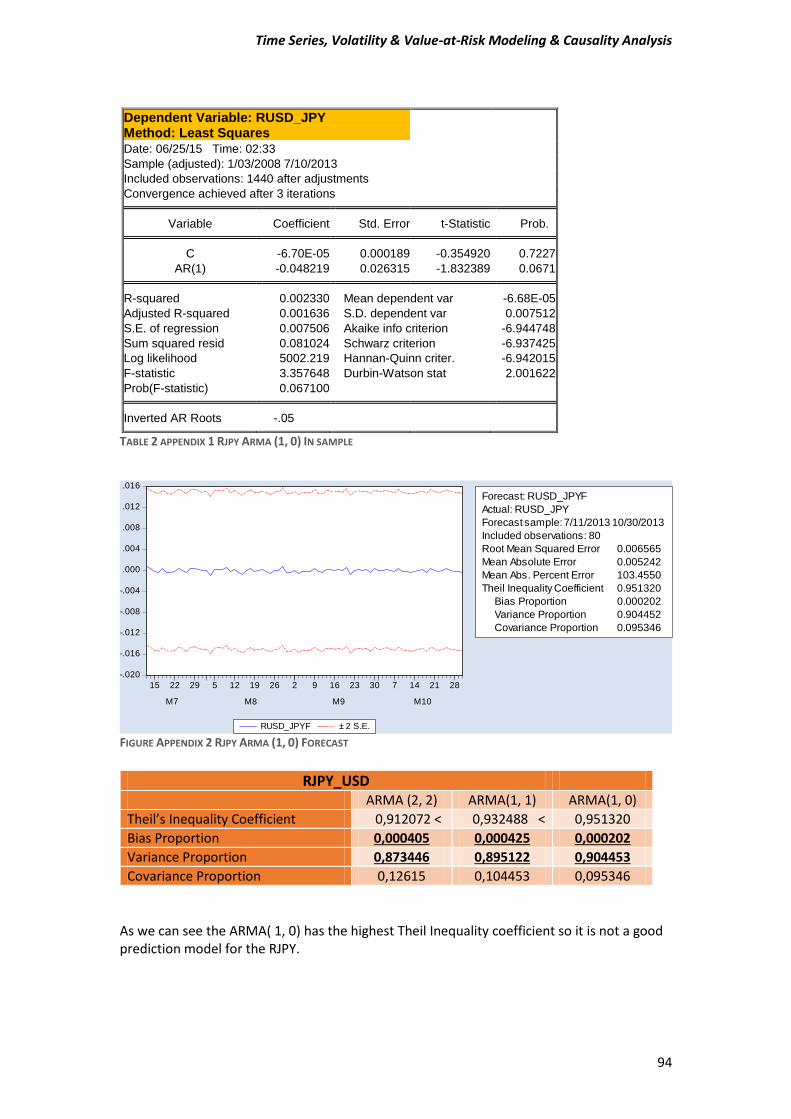
Time Series, Volatility & Value-at-Risk Modeling & Causality Analysis
94
Dependent Variable: RUSD_JPY
Method: Least Squares
Date: 06/25/15 Time: 02:33
Sample (adjusted): 1/03/2008 7/10/2013
Included observations: 1440 after adjustments
Convergence achieved after 3 iterations Variable Coefficient Std. Error t-Statistic Prob. C -6.70E-05 0.000189 -0.354920 0.7227
AR(1) -0.048219 0.026315 -1.832389 0.0671 R-squared 0.002330 Mean dependent var -6.68E-05
Adjusted R-squared 0.001636 S.D. dependent var 0.007512
S.E. of regression 0.007506 Akaike info criterion -6.944748
Sum squared resid 0.081024 Schwarz criterion -6.937425
Log likelihood 5002.219 Hannan-Quinn criter. -6.942015
F-statistic 3.357648 Durbin-Watson stat 2.001622
Prob(F-statistic) 0.067100 Inverted AR Roots -.05
TABLE 2 APPENDIX 1 RJPY ARMA (1, 0) IN SAMPLE
FIGURE APPENDIX 2 RJPY ARMA (1, 0) FORECAST
As we can see the ARMA( 1, 0) has the highest Theil Inequality coefficient so it is not a good prediction model for the RJPY.
-.020
-.016
-.012
-.008
-.004
.000
.004
.008
.012
.016
15 22 29 5 12 19 26 2 9 16 23 30 7 14 21 28
M7 M8 M9 M10
RUSD_JPYF ± 2 S.E.
Forecast: RUSD_JPYF
Actual: RUSD_JPY
Forecast sample: 7/11/2013 10/30/2013
Included observations: 80
Root Mean Squared Error 0.006565
Mean Absolute Error 0.005242
Mean Abs. Percent Error 103.4550
Theil Inequality Coefficient 0.951320
Bias Proportion 0.000202
Variance Proportion 0.904452
Covariance Proportion 0.095346
RJPY_USD ARMA (2, 2) ARMA(1, 1) ARMA(1, 0)
Theil’s Inequality Coefficient 0,912072 < 0,932488 < 0,951320
Bias Proportion 0,000405 0,000425 0,000202
Variance Proportion 0,873446 0,895122 0,904453
Covariance Proportion 0,12615 0,104453 0,095346
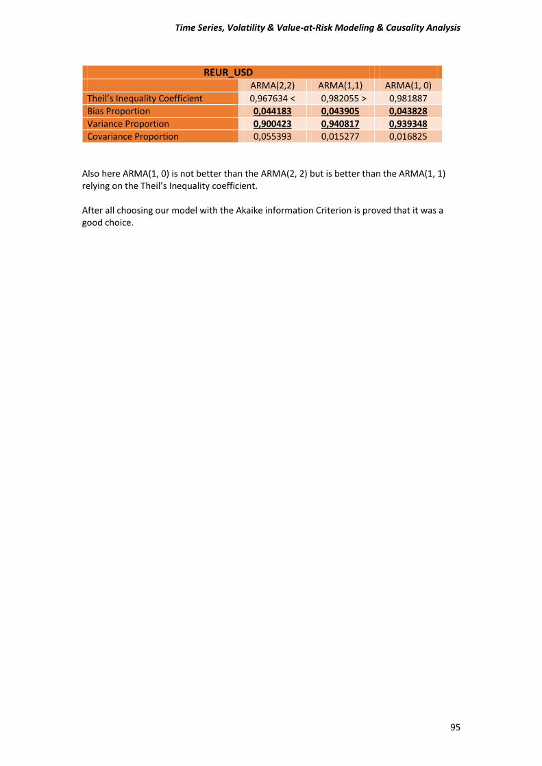
Time Series, Volatility & Value-at-Risk Modeling & Causality Analysis
95
Also here ARMA(1, 0) is not better than the ARMA(2, 2) but is better than the ARMA(1, 1) relying on the Theil’s Inequality coefficient. After all choosing our model with the Akaike information Criterion is proved that it was a good choice.
REUR_USD ARMA(2,2) ARMA(1,1) ARMA(1, 0)
Theil’s Inequality Coefficient 0,967634 < 0,982055 > 0,981887
Bias Proportion 0,044183 0,043905 0,043828
Variance Proportion 0,900423 0,940817 0,939348
Covariance Proportion 0,055393 0,015277 0,016825
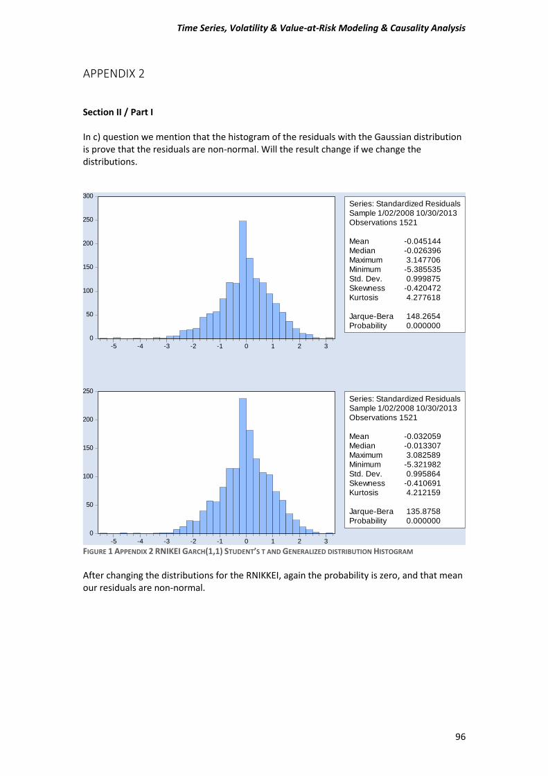
Time Series, Volatility & Value-at-Risk Modeling & Causality Analysis
96
APPENDIX 2 Section II / Part I In c) question we mention that the histogram of the residuals with the Gaussian distribution is prove that the residuals are non-normal. Will the result change if we change the distributions.
FIGURE 1 APPENDIX 2 RNIKEI GARCH(1,1) STUDENT’S T AND GENERALIZED DISTRIBUTION HISTOGRAM After changing the distributions for the RNIKKEI, again the probability is zero, and that mean our residuals are non-normal.
0
50
100
150
200
250
300
-5 -4 -3 -2 -1 0 1 2 3
Series: Standardized Residuals
Sample 1/02/2008 10/30/2013
Observations 1521
Mean -0.045144
Median -0.026396
Maximum 3.147706
Minimum -5.385535
Std. Dev. 0.999875
Skewness -0.420472
Kurtosis 4.277618
Jarque-Bera 148.2654
Probability 0.000000
0
50
100
150
200
250
-5 -4 -3 -2 -1 0 1 2 3
Series: Standardized Residuals
Sample 1/02/2008 10/30/2013
Observations 1521
Mean -0.032059
Median -0.013307
Maximum 3.082589
Minimum -5.321982
Std. Dev. 0.995864
Skewness -0.410691
Kurtosis 4.212159
Jarque-Bera 135.8758
Probability 0.000000
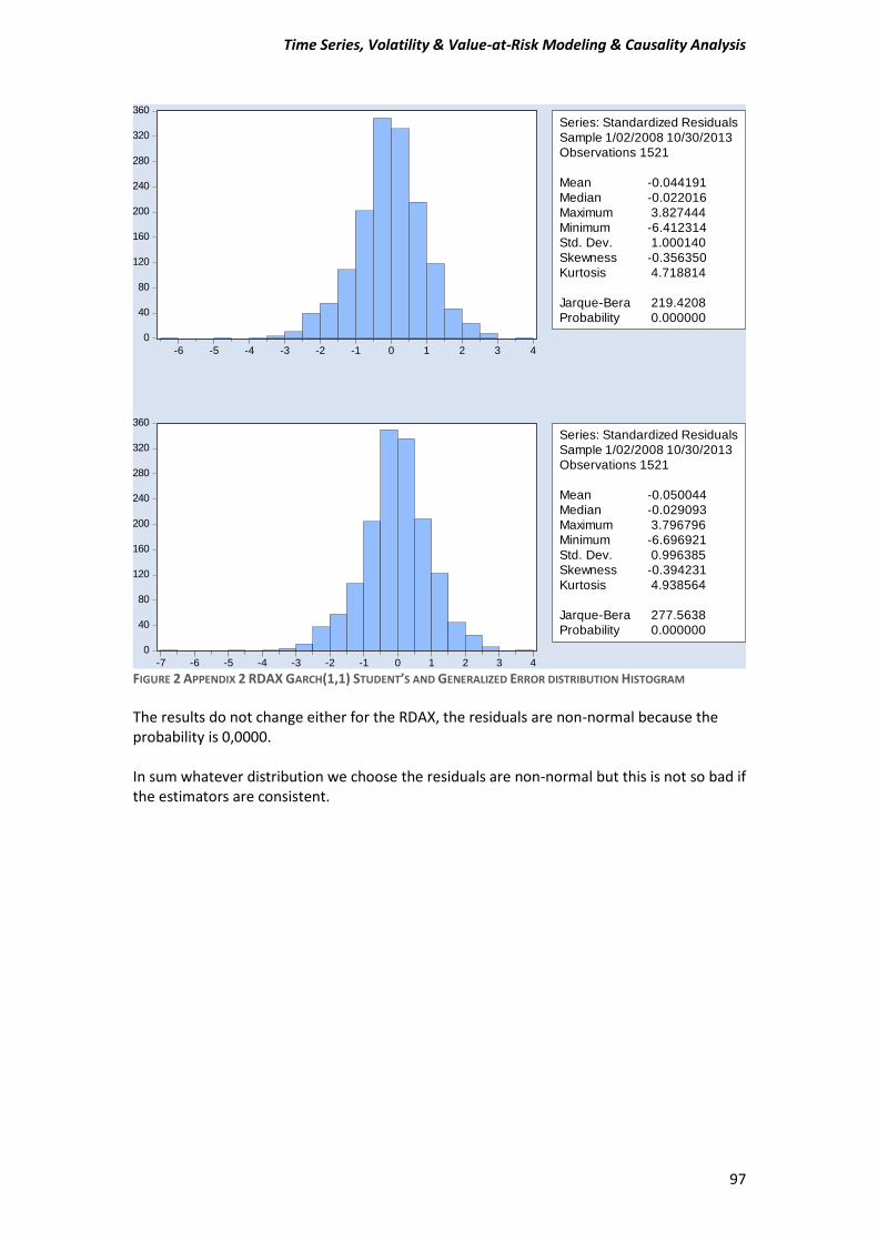
Time Series, Volatility & Value-at-Risk Modeling & Causality Analysis
97
FIGURE 2 APPENDIX 2 RDAX GARCH(1,1) STUDENT’S AND GENERALIZED ERROR DISTRIBUTION HISTOGRAM
The results do not change either for the RDAX, the residuals are non-normal because the probability is 0,0000. In sum whatever distribution we choose the residuals are non-normal but this is not so bad if the estimators are consistent.
0
40
80
120
160
200
240
280
320
360
-6 -5 -4 -3 -2 -1 0 1 2 3 4
Series: Standardized Residuals
Sample 1/02/2008 10/30/2013
Observations 1521
Mean -0.044191
Median -0.022016
Maximum 3.827444
Minimum -6.412314
Std. Dev. 1.000140
Skewness -0.356350
Kurtosis 4.718814
Jarque-Bera 219.4208
Probability 0.000000
0
40
80
120
160
200
240
280
320
360
-7 -6 -5 -4 -3 -2 -1 0 1 2 3 4
Series: Standardized Residuals
Sample 1/02/2008 10/30/2013
Observations 1521
Mean -0.050044
Median -0.029093
Maximum 3.796796
Minimum -6.696921
Std. Dev. 0.996385
Skewness -0.394231
Kurtosis 4.938564
Jarque-Bera 277.5638
Probability 0.000000
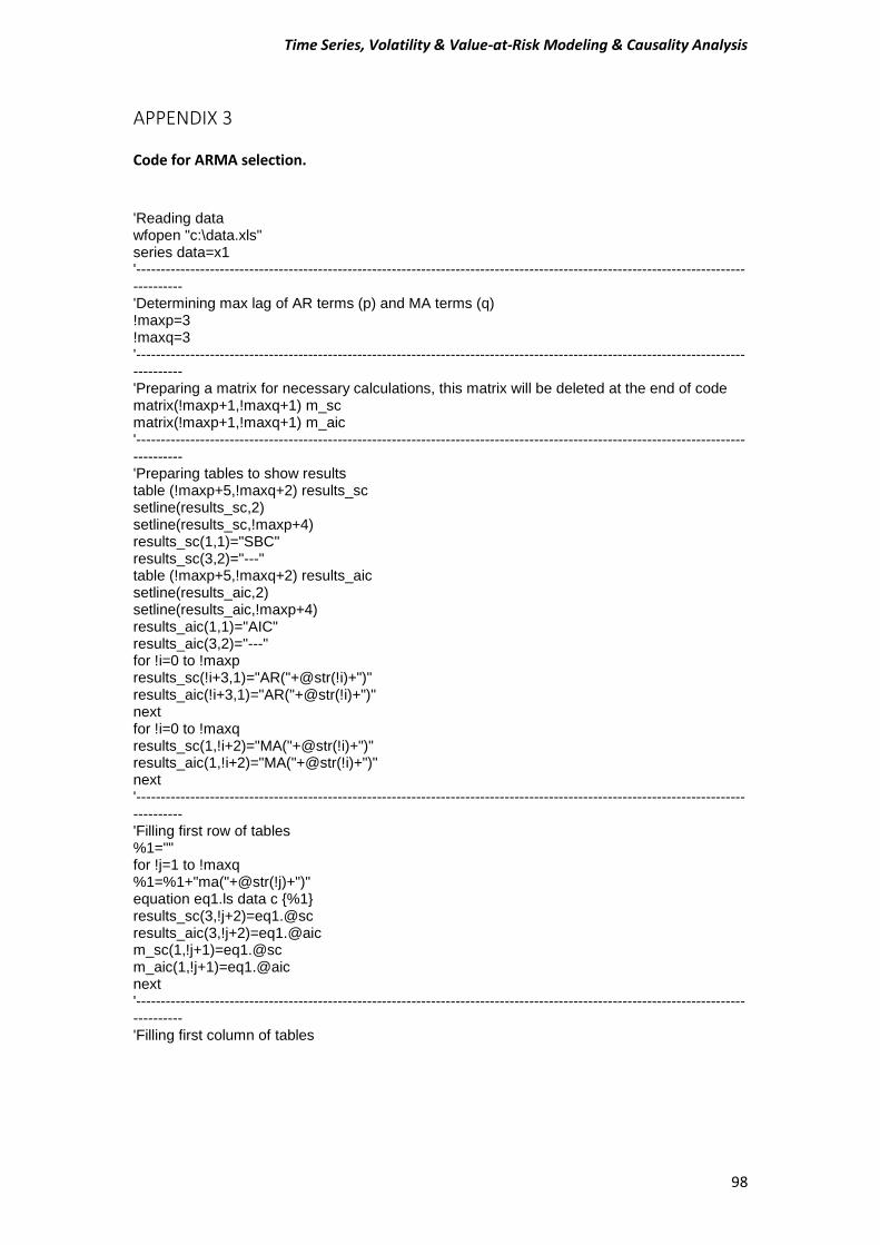
Time Series, Volatility & Value-at-Risk Modeling & Causality Analysis
98
APPENDIX 3 Code for ARMA selection. 'Reading data wfopen "c:\data.xls" series data=x1 '-------------------------------------------------------------------------------------------------------------------------------------- 'Determining max lag of AR terms (p) and MA terms (q) !maxp=3 !maxq=3 '-------------------------------------------------------------------------------------------------------------------------------------- 'Preparing a matrix for necessary calculations, this matrix will be deleted at the end of code matrix(!maxp+1,!maxq+1) m_sc matrix(!maxp+1,!maxq+1) m_aic '-------------------------------------------------------------------------------------------------------------------------------------- 'Preparing tables to show results table (!maxp+5,!maxq+2) results_sc setline(results_sc,2) setline(results_sc,!maxp+4) results_sc(1,1)="SBC" results_sc(3,2)="---" table (!maxp+5,!maxq+2) results_aic setline(results_aic,2) setline(results_aic,!maxp+4) results_aic(1,1)="AIC" results_aic(3,2)="---" for !i=0 to !maxp results_sc(!i+3,1)="AR("+@str(!i)+")" results_aic(!i+3,1)="AR("+@str(!i)+")" next for !i=0 to !maxq results_sc(1,!i+2)="MA("+@str(!i)+")" results_aic(1,!i+2)="MA("+@str(!i)+")" next '-------------------------------------------------------------------------------------------------------------------------------------- 'Filling first row of tables %1="" for !j=1 to !maxq %1=%1+"ma("+@str(!j)+")" equation eq1.ls data c {%1} results_sc(3,!j+2)=eq1.@sc results_aic(3,!j+2)=eq1.@aic m_sc(1,!j+1)=eq1.@sc m_aic(1,!j+1)=eq1.@aic next '-------------------------------------------------------------------------------------------------------------------------------------- 'Filling first column of tables
Time Series, Volatility & Value-at-Risk Modeling & Causality Analysis
99
%2="" for !k=1 to !maxp %2=%2+"ar("+@str(!k)+")" equation eq2.ls data c {%2} results_sc(!k+3,2)=eq2.@sc results_aic(!k+3,2)=eq2.@aic m_sc(!k+1,1)=eq2.@sc m_aic(!k+1,1)=eq2.@aic next '-------------------------------------------------------------------------------------------------------------------------------------- 'Filling other parts of tables %3="" for !p=1 to !maxp %3=%3+"ar("+@str(!p)+")" %4="" for !q=1 to !maxq %4=%4+"ma("+@str(!q)+")" %5=%3+%4 equation eq.ls data c {%5} results_sc(!p+3,!q+2)=eq.@sc results_aic(!p+3,!q+2)=eq.@aic m_sc(!p+1,!q+1)=eq.@sc m_aic(!p+1,!q+1)=eq.@aic next next '-------------------------------------------------------------------------------------------------------------------------------------- 'Determining the bestmodel !pq=@max(m_sc) m_sc(1,1)=!pq !pq=@max(m_aic) m_aic(1,1)=!pq !maxpp=!maxp+1 !maxqq=!maxq+1 !pq=@min(m_sc) for !pp=1 to !maxpp for !qq=1 to !maxqq if m_sc(!pp,!qq)=!pq then !finalp=!pp-1 !finalq=!qq-1 endif next next results_sc(!maxp+5,1)="Best Model Is ARMA("+@str(!finalp)+","+@str(!finalq)+")" !pq=@min(m_aic) for !pp=1 to !maxpp for !qq=1 to !maxqq if m_aic(!pp,!qq)=!pq then !finalp=!pp-1 !finalq=!qq-1 endif next next results_aic(!maxp+5,1)="Best Model Is ARMA("+@str(!finalp)+","+@str(!finalq)+")" '-------------------------------------------------------------------------------------------------------------------------------------- 'Deleting excess data delete eq eq1 eq2 m_sc m_aic

Time Series, Volatility & Value-at-Risk Modeling & Causality Analysis
100
'-------------------------------------------------------------------------------------------------------------------------------------- 'Showing results show results_sc show results_aic
In additions, for the ARMA selection model, also used an Add-In which is called ARIMASEL. The Add-in was abstracted from the http://www.eviews.com/Addins/addins.shtml .