echT PressScienceComputers, Materials & ContinuaDOI:10.32604/cmc.2021.016893

Article

Enhanced Accuracy for Motor Imagery Detection Using Deep Learning for BCI

Ayesha Sarwar1, Kashif Javed1, Muhammad Jawad Khan1, Saddaf Rubab1,Oh-Young Song2,* and Usman Tariq3

1National University of Sciences and Technology (NUST), Islamabad, 44000, Pakistan2Department of Software, Sejong University, Seoul, Gwangjin-gu, Korea

3College of Computer Engineering and Sciences, Prince Sattam bin Abdulaziz University, Al-Kharj, 11942, Saudi Arabia*Corresponding Author: Oh-Young Song. Email: oysong@sejong.ac.kr

Received: 14 January 2021; Accepted: 01 March 2021

Abstract: Brain-Computer Interface (BCI) is a system that provides a linkbetween the brain of humans and the hardware directly. The recorded braindata is converted directly to the machine that can be used to control externaldevices. There are four major components of the BCI system: acquiring sig-nals, preprocessing of acquired signals, features extraction, and classification.In traditional machine learning algorithms, the accuracy is insignificant andnot up to the mark for the classification of multi-class motor imagery data.The major reason for this is, features are selected manually, and we are notable to get those features that give higher accuracy results. In this study, motorimagery (MI) signals have been classified using different deep learning algo-rithms. We have explored two different methods: Artificial Neural Network(ANN) and Long Short-Term Memory (LSTM). We test the classificationaccuracy on two datasets: BCI competition III-dataset IIIa and BCI com-petition IV-dataset IIa. The outcome proved that deep learning algorithmsprovide greater accuracy results than traditional machine learning algorithms.Amongst the deep learning classifiers, LSTMoutperforms the ANN and giveshigher classification accuracy of 96.2%.

Keywords: Brain-computer interface; motor imagery; artificial neuralnetwork; long-short term memory; classification

1 Introduction

Brain-Computer Interface (BCI) is a developing field of exploration that seeks to upgradethe effectiveness and level of computer applications centered on the human. A Brain-ComputerInterface based on Motor Imagery (MI) offers ways to express your thoughts to an externalsystem without any vocal communication. For the last two to three decades BCI has gainedresearcher’s attention and extensive work is done in this field [1–3]. There are many applicationsof BCI like medicine, education, games, entertainment, and human-computer interaction [4–6].BCI systems based on motor imagery signals have received a lot of heed in the field of assistivetechnology. There are two major application categories where MI-based systems are majorly usedi.e., for motor action replacement or as a recovery system for motor action recovery.

This work is licensed under a Creative Commons Attribution 4.0 International License,which permits unrestricted use, distribution, and reproduction in any medium, providedthe original work is properly cited.

3826 CMC, 2021, vol.68, no.3

A BCI framework contains the following components: signal acquiring, signal processingextraction of features, and classification [7]. In Fig. 1, the key components of a BCI system areshown. Whereas, the electrical activity of the brain is recorded in the first part by conducting anexperiment or performing some voluntary tasks. Brain signals may be obtained either by invasiveor non-invasive approaches. The positioning of electrodes is on the surface of the brain for signalacquisition purposes in the invasive process while in a non-invasive procedure signals are acquiredwithout performing any surgical intervention. With an invasive method, the acquired signal is ofbetter quality, but we prefer the non-invasive method due to its ease of use and implementation.Electroencephalogram (EEG) is one of the most commonly used methods of signal acquiringbecause of its non-invasive nature, cheapness, and ease of usage. A German psychiatrist HansBerger for the first time recorded the EEG signals in 1924. EEG is a technique in which electricalimpulses from the brain are measured by putting a series of electrodes on the human brain’ssurface. The brain signals gather through EEG are then pre-processed. The feature extraction isthe next important step after the pre-processing of signals. Different types of features can beremoved from pre-processed signals by adopting different feature extraction methods. The featuresthat have been extracted are then given to the classifier for its training. Based on feature values,the trained classifier classifies the human intended actions into one of the predefined classes. Theselection of desirable features to obtain the necessary classification results is one of the mainchallenges in the BCI study.

Figure 1: Major components of the BCI system

In traditional machine learning algorithms, the accuracy achieved for the classification ofmulti-class motor imagery data is insignificant and not up to the mark. The major reason isas features are selected manually, and we are not able to get those features that provide highaccuracy results. To overcome this challenge, we proposed an efficient deep learning algorithm.Our contribution included in this article is as follow:

(1) A deep learning approach that can be used to manually extract features for the motorimagery signals. The network learns to extract features while training and we just have tofeed the signals dataset to the network.

(2) By deploying Artificial Neural Network (ANN) and Long Short-Term Memory (LSTM)deep learning algorithms for extracting motor imagery-based features.

2 Related Work

Enhanced accuracy for motor imagery detection is a challenging research area in the field ofdeep learning (DL). For achieving the best accuracy results the desired features are unknown inmost of the studies [8]. In the traditional machine learning approach, the features are extractedmanually and fed to train the classifier, and we are not able to get those features that provide

CMC, 2021, vol.68, no.3 3827

high accuracy results. Many traditional machine algorithms have already been implemented forthe classification of brain signals like support vector machine (SVM) [9], multilayer perceptron(MLP) [10], linear discriminant analysis (LDA) [11].

In another study [8], traditional classifiers like k-NN, SVM, MLP were applied for theclassification of signals; the accuracies achieved were not significant enough. In a recent study [12]on EEG data for the classification of motor imagery comparison of traditional and deep learningclassifiers was made, the results showed higher accuracies for deep learning classifiers. In our work,we deal with the classification component from brain-computer interface systems with a majorfocus on deep learning algorithms. In past studies [8], deep learning algorithms have providedbetter accuracy results in contrast to machine learning algorithms. [13,14] presents different casestudies related to machine learning and deep neural networking models. In the deep learningapproach, there is no need to manually obtain features from pre-processed signals, the networkitself learns to extract the features while training and we just have to feed the dataset to thenetwork. In our study, we analyzed the performance of an artificial neural network (ANN) [15–17]and recurrent neural network (RNN) [18]. Moreover, we implemented long short-term memory(LSTM) [19] in the recurrent neural network. LSTM outperforms ANN and provides higheraccuracy results with 96.2%.

During the last decade, a variety of publications have been reported for the classification ofmulti-class datasets that make use of deep learning [13,14,20,21]. Steady-State Visually EvokedPotential (SSVEP) was used for the classification of EEG based signals in a study [22]. In thiswork, the subjects were introduced to visual cues at a particular frequency. The accuracy achievedwas 97% but the used criteria for reliability rejection was the problem, which resulted in therejection of a large number of samples resulting in average results. For the classification of data inBCI applications, different approaches have been used like learning vector quantization (LVQ) [23]and CNN [24]. In another study [25], RNN is used for the classification of motor imagery EEG-based data set the accuracy achieved was 79.6% and wavelet filter was used. In a recent work [26],CNN-LSTM based deep learning classifier was used and the maximum test accuracy was targetedat 86.8%. EEG signals were extracted using low cost and invasive headbands in the study.

The next Section 3 summaries the detail of the datasets used in this work, their time paradigmfor the collection of raw data from the experiment, and pre-processing steps applied to the rawdataset. After datasets, there is an explanation of both the architectures used in this work. Thedetailed accuracy results of both the datasets using different architectures and window sizes alongwith their accuracy and loss graphs are presented in Section 4. Conclusions and discussion aredescribed in Section 5.

3 Methods

In this section, we have discussed all the datasets used in this work, their preprocessing. Thedatasets involved in the BCI dataset and preprocessing include competition III, dataset IIIa andBCI competition IV, dataset IIa. There is a discussion on the time paradigm and steps involvedin the preprocessing of both datasets. Afterward, we have discussed the methodology that hasbeen used in this study. We worked on two algorithms i.e., Artificial Neural Network (ANN) andLong-Short Term Memory (LSTM) for the classification of the datasets. The details are discussedlater in this section.

3828 CMC, 2021, vol.68, no.3

3.1 BCI Dataset and PreprocessingThere are two MI-based four-class datasets used in this work. Both the datasets consist of

multiple subjects. The four-class motor imagery corresponds to the MI movement i.e., the righthand, left hand, tongue, and feet. The first dataset used is the IIIa dataset [27] from the thirdcompetition of BCI and it comprises 3 subjects. The second dataset IIa [28,29] is from the fourthBCI competition and it consists of 9 subjects. Both the datasets used in this work were availablepublicly by the Graz University of Technology. Based on a visual cue shown to the participants,all the subjected were asked to carry out four unalike imagery tasks during the experiment. In thenext section, there is a detail of both the datasets used, their design.

3.1.1 BCI Competition III, Dataset IIIa1) Paradigm

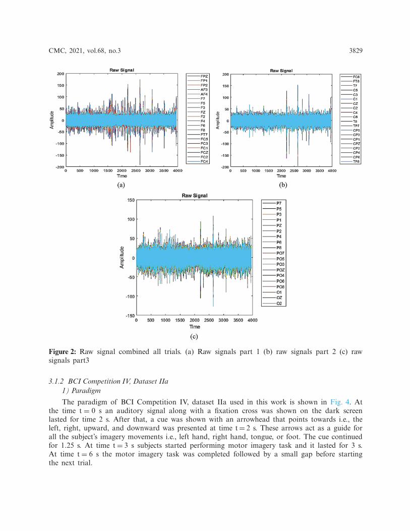
The experiment starts with the subject sitting on a relaxing chair. According to a cue, imagerymovements i.e.„ left hand, right hand, tongue, and foot were asked to perform. The cues wereshown randomly. There were 6 runs and each run contained 40 trials. Each trial comprises of8 s in total. The first 2 s were blank and quiet, at time = 2 s a cue (beep sound) indicates thestart of a trial. An arrow symbol was displayed at time t= 3 s for 1s, which points towards theleft, right, up, or down. In the meanwhile, the participants were trained to imagine the left hand,the right hand, feet, and tongue imagery. This process of imagery ends at t= 7 s until the crossdisappeared. Subject 1 of this experiment K3 consisted of a total of 9 runs, which result in 360trials in total for K3. There were 90 trials for each class. From these 360 trials, 180 trials werefor training and 180 for evaluation purposes. For subject 2 (K6) and subject 3 (L1), there weresix runs each, leading to 240 trials for each subject. For subjects K6 and L1, there were 60 trialseach. Data from training and assessment comprises of 120 trials each (30 trials for each class).Fig. 2, shows the raw signal for a single subject. It includes all the trial data of a subject. Eachcolor in the figure represents a channel or electrode placement on the scalp. In Fig. 2a first 20channels are presented in different colors and in the same way in Figs. 2b and 2c remaining 21–40and 41–60 channels are represented respectively. The labels are described in Tab. 1.

2) Pre-processing

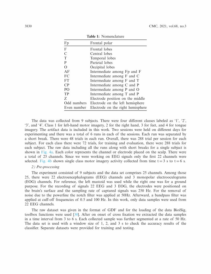
A 64-channel electroencephalogram (EEG) amplifier from Neuroscan was used to record datafor all the subjects. The left mastoid was used as a reference, and the ground was used for the rightone. For the recording of signals, there were 60 electrodes based on EEG that were positioned onthe surface of the brain. The EEG signals captured were tested at 250 Hz. For removing noisedue to the power line after filtering the signals at 50 Hz, a notch filter was used. The raw andfiltered signals are shown in Fig. 3. The raw signal for the single electrode is shown in Fig. 3dand after applying the filter the resultant signal is shown in Fig. 3e.

The trials with artifacts were also included. Trig value in data tells about the start of eachtrial and Class Label gave information about the classes that were labeled as “1” as the left hand,“2” as the right hand, “3” as the tongue, and “4” as the foot. For our work data of the firstthree seconds is removed and data from time t= 3 s till time t= 7 s is collected where the motorimagery movement occurs. Figs. 3a–3c there is a display of channels of single-trial of one class.The trial includes a 4 s motor imagery activity part. A sample of size 4s with 60 channels iscollected. Each sample is segmented further with a sampling rate of 50 Hz.

CMC, 2021, vol.68, no.3 3829

Figure 2: Raw signal combined all trials. (a) Raw signals part 1 (b) raw signals part 2 (c) rawsignals part3

3.1.2 BCI Competition IV, Dataset IIa1) Paradigm

The paradigm of BCI Competition IV, dataset IIa used in this work is shown in Fig. 4. Atthe time t = 0 s an auditory signal along with a fixation cross was shown on the dark screenlasted for time 2 s. After that, a cue was shown with an arrowhead that points towards i.e., theleft, right, upward, and downward was presented at time t= 2 s. These arrows act as a guide forall the subject’s imagery movements i.e., left hand, right hand, tongue, or foot. The cue continuedfor 1.25 s. At time t= 3 s subjects started performing motor imagery task and it lasted for 3 s.At time t = 6 s the motor imagery task was completed followed by a small gap before startingthe next trial.

3830 CMC, 2021, vol.68, no.3

Table 1: Nomenclature

Fp Frontal polar

F Frontal lobesC Central lobesT Temporal lobesP Parietal lobesO Occipital lobesAF Intermediate among Fp and FFC Intermediate among F and CFT Intermediate among F and TCP Intermediate among C and PPO Intermediate among P and OTP Intermediate among T and PZ Electrode position on the middleOdd numbers Electrode on the left hemisphereEven number Electrode on the right hemisphere

The data was collected from 9 subjects. There were four different classes labeled as ‘1’, ‘2’,‘3’, and ‘4’. Class 1 for left-hand motor imagery, 2 for the right hand, 3 for feet, and 4 for tongueimagery. The artifact data is included in this work. Two sessions were held on different days forexperimenting and there was a total of 6 runs in each of the sessions. Each run was separated bya short break. There were 48 trials in each run. Overall, there was 288 trial per session for eachsubject. For each class there were 72 trials, for training and evaluation, there were 288 trials foreach subject. The raw data including all the runs along with short breaks for a single subject isshown in Fig. 4a. Each color represents the channel or electrode placed on the scalp. There werea total of 25 channels. Since we were working on EEG signals only the first 22 channels wereselected. Fig. 4b shown single class motor imagery activity collected from time t= 3 s to t= 6 s.

2) Pre-processing

The experiment consisted of 9 subjects and the data set comprises 25 channels. Among those25, there were 22 electroencephalograms (EEG) channels and 3 monopolar electrooculograms(EOG) channels. For reference, the left mastoid was used while the right one was for a groundpurpose. For the recording of signals 22 EEG and 3 EOG, the electrodes were positioned onthe brain’s surface and the sampling rate of captured signals was 250 Hz. For the removal ofnoise due to the powerline the notch filter was applied at 50Hz. Afterward, a bandpass filter wasapplied at cuff-off frequencies of 0.5 and 100 Hz. In this work, only data samples were used from22 EEG channels.

The raw dataset was given in the format of GDF and for the loading of the data BioiSig,toolbox functions were used [30]. After on onset of cross fixation we extracted the data samplesin a time interval from 3 to 6 s. Each collected sample was further segmented at a rate of 50 Hz.The data set is used with a window size of 1, 2, and 3 s to check the accuracy results of theclassifier. Separate datasets were provided for training and testing.

CMC, 2021, vol.68, no.3 3831

Figure 3: Raw and Filtered Signals. (a) Single class trial part 1 (b) single class trial part 2 (c)single class trial part 3 (d) raw signal (e) filtered signal

3832 CMC, 2021, vol.68, no.3

Figure 4: Raw data. (a) Raw data of all trials (b) single trial data

3.2 Adopted MethodologyThe methodology that was adopted for this work is shown in Fig. 5. Data acquisition and

data preprocessing have been discussed in the previous section. After gathering the preprocessedsignals the next step is choosing the architecture. In this work, we have used ANN and LSTMarchitecture for the classification of motor imagery datasets. After selecting the appropriate archi-tecture we trained the model. Then the test datasets were passes to the trained model to get theaccuracy results for both the architectures. The architectures used in this work and the accuracyresults are discussed in later sections.

3.3 Deep Learning MethodIn deep neural networks, several layers of neurons are arranged over each other. The per-

formance of the network can be improved by adding hidden layers to the network [31]. As thenumber of layers increases the complexity of the network increases. The major advantage of deeplearning algorithms is there is no need to manually extract features which is a challenging taskin the machine learning method. We just have to feed the dataset to the network it automaticallylearns the features. In this work we use two methods; we worked on ANN and RNN withLSTM architecture.

3.3.1 Artificial Neural Network (ANN)The ANN is a feed-forward network consisted of various layers [32]. Backpropagation is used

to update the weights. The architecture comprises 10 layers. There are the following different typesof layers in this architecture: an input layer, a ReLU layer, and fully connected dense layers.The network has an input layer that is then converted to a one-dimensional array and connectedto eight fully connected dense hidden layers. In each hidden layer, the neurons depend on theinputs of the input layer. In these layers, input and output are linked through a learnable weight.Each connected layer is also passed through non-linear activation functions such as ReLU. Thefinal layer typically has the same number of nodes as the number of classes the input datamust be classified into. The last layer’s activation function is chosen very carefully and is usuallydifferent from previous fully connected layers. One of the most commonly used layers is SoftMax,which normalizes the results between 0 and 1 based on the probability of each class. Typically,

CMC, 2021, vol.68, no.3 3833

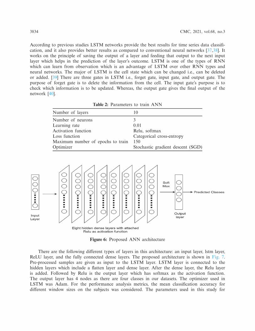
neural networks are updates by stochastic gradient descent. The training algorithm was chosenas stochastic gradient descent (SGD). The size of the batch was set to 64 and the layers. Allthe hyperparameters like the number of neurons, learning rate, weights, optimizer, and batch sizewere chosen empirically with repeated network training for achieving optimized accuracy results.The accuracy results are greatly affected by the selection of hyper-parameters [33] and the hyper-parameters used in this study are shown in Tab. 2. It is convenient to adjust the training iterationsfreely [34]. Apart from hyperparameters mentioned, Bayesian optimization can also be utilizedto improve the overall performance of the system. In our work, the model was trained on 150epochs. For this specific study, the learning rate selected was 0.01. A larger learning rate causesdivergence in the network inversely, the smaller the learning rate network convergence will beslow. For the performance analysis metrics, the mean classification accuracy for different windowsizes on the subjects was considered. A deep learning approach was used as we do not need tomanually extract features for the motor imagery signals. The network learns to extract featureswhile training and we just have to feed the signals dataset to the network. As in CNN and RNN,more data inputs or features are required to achieve the better accuracy as compared to ANN.However, the proposed method has employed deep learning approach using ANN as it does notrequire to extract many features. The architecture used in this study is shown in Fig. 6.

Figure 5: Flow chart for adopted methodology

3.3.2 Long Short-Term Memory (LSTM)The other Architecture that we are using for exploring the classification of EEG signals

is long short-term memory (LSTM). It is one of the types of recurrent neural networks. TheRecurrent Neural networks were initially represented by Schmidhuber’s research group [35,36].

3834 CMC, 2021, vol.68, no.3

According to previous studies LSTM networks provide the best results for time series data classifi-cation, and it also provides better results as compared to conventional neural networks [37,38]. Itworks on the principle of saving the output of a layer and feeding that output to the next inputlayer which helps in the prediction of the layer’s outcome. LSTM is one of the types of RNNwhich can learn from observation which is an advantage of LSTM over other RNN types andneural networks. The major of LSTM is the cell state which can be changed i.e., can be deletedor added. [39] There are three gates in LSTM i.e., forget gate, input gate, and output gate. Thepurpose of forget gate is to delete the information from the cell. The input gate’s purpose is tocheck which information is to be updated. Whereas, the output gate gives the final output of thenetwork [40].

Table 2: Parameters to train ANN

Number of layers 10

Number of neurons 3Learning rate 0.01Activation function Relu, softmaxLoss function Categorical cross-entropyMaximum number of epochs to train 150Optimizer Stochastic gradient descent (SGD)

Figure 6: Proposed ANN architecture

There are the following different types of layers in this architecture: an input layer, lstm layer,ReLU layer, and the fully connected dense layers. The proposed architecture is shown in Fig. 7.Pre-processed samples are given as input to the LSTM layer. LSTM layer is connected to thehidden layers which include a flatten layer and dense layer. After the dense layer, the Relu layeris added. Followed by Relu is the output layer which has softmax as the activation function.The output layer has 4 nodes as there are four classes in our datasets. The optimizer used inLSTM was Adam. For the performance analysis metrics, the mean classification accuracy fordifferent window sizes on the subjects was considered. The parameters used in this study for

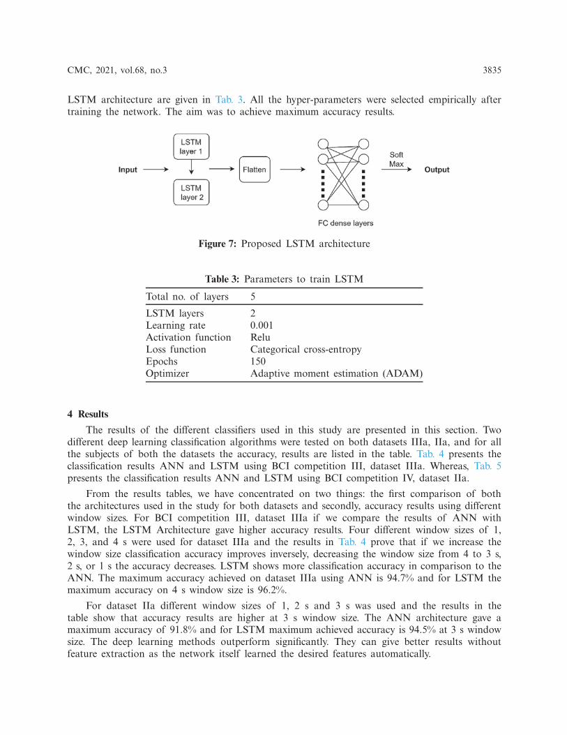
CMC, 2021, vol.68, no.3 3835

LSTM architecture are given in Tab. 3. All the hyper-parameters were selected empirically aftertraining the network. The aim was to achieve maximum accuracy results.

Figure 7: Proposed LSTM architecture

Table 3: Parameters to train LSTM

Total no. of layers 5

LSTM layers 2Learning rate 0.001Activation function ReluLoss function Categorical cross-entropyEpochs 150Optimizer Adaptive moment estimation (ADAM)

4 Results

The results of the different classifiers used in this study are presented in this section. Twodifferent deep learning classification algorithms were tested on both datasets IIIa, IIa, and for allthe subjects of both the datasets the accuracy, results are listed in the table. Tab. 4 presents theclassification results ANN and LSTM using BCI competition III, dataset IIIa. Whereas, Tab. 5presents the classification results ANN and LSTM using BCI competition IV, dataset IIa.

From the results tables, we have concentrated on two things: the first comparison of boththe architectures used in the study for both datasets and secondly, accuracy results using differentwindow sizes. For BCI competition III, dataset IIIa if we compare the results of ANN withLSTM, the LSTM Architecture gave higher accuracy results. Four different window sizes of 1,2, 3, and 4 s were used for dataset IIIa and the results in Tab. 4 prove that if we increase thewindow size classification accuracy improves inversely, decreasing the window size from 4 to 3 s,2 s, or 1 s the accuracy decreases. LSTM shows more classification accuracy in comparison to theANN. The maximum accuracy achieved on dataset IIIa using ANN is 94.7% and for LSTM themaximum accuracy on 4 s window size is 96.2%.

For dataset IIa different window sizes of 1, 2 s and 3 s was used and the results in thetable show that accuracy results are higher at 3 s window size. The ANN architecture gave amaximum accuracy of 91.8% and for LSTM maximum achieved accuracy is 94.5% at 3 s windowsize. The deep learning methods outperform significantly. They can give better results withoutfeature extraction as the network itself learned the desired features automatically.

3836 CMC, 2021, vol.68, no.3

Table 4: Classification accuracies for dataset IIIa using different window sizes

Architecture Window size (s) K3 K6 L1 Average

ANN 4 0.961 0.941 0.946 0.947ANN 3 0.933 0.921 0.929 0.927ANN 2 0.920 0.911 0.915 0.915ANN 1 0.851 0.820 0.842 0.831LSTM 4 0.960 0.961 0.952 0.962LSTM 3 0.947 0.948 0.955 0.949LSTM 2 0.921 0.920 0.929 0.925LSTM 1 0.880 0.870 0.876 0.870

Table 5: Classification accuracies for dataset IIa using different window sizes

Architecture Windowsize (s) A1 A2 A3 A4 A5 A6 A7 A8 A9 Accuracy

LSTM 3 .947 .933 .949 .945 .946 .947 .949 .948 .947 .945LSTM 2 .921 .915 .923 .918 .920 .919 .923 .921 .911 .919LSTM 1 .845 .838 .847 .840 .843 .841 .844 .845 .838 .842ANN 3 .919 .916 .920 .919 .920 .917 .922 .919 .918 .918ANN 2 .867 .859 .871 .865 .866 .878 .873 .876 .865 .868ANN 1 .828 .817 .825 .823 .824 .826 .827 .826 .819 .823

Accuracy and loss plots for the datasets for ANN are shown in Figs. 8a, 8b, and for LSTMin Figs. 9a and 9b. Accuracy plots show that’s as the number of epochs increases the training andtest accuracy increases and after a certain number of epochs it increases to its maximum value.The green color shows the training accuracy while blue shows the test accuracy. For loss plots inFigs. 8b and 9b loss value decrease as the training, iterations are increasing, and after a certainepoch, loss reaches its minimum value.

Figure 8: Accuracy and loss graphs for ANN: (a) Accuracy graph for ANN (b) loss graphfor ANN

CMC, 2021, vol.68, no.3 3837

Figure 9: Accuracy and loss graphs for LSTM: (a) Accuracy graph for LSTM (b) accuracy andloss graph for LSTM

5 Discussion and Conclusions

We have explored the classification algorithms for four-class motor imagery-based EEG sig-nals. The target of the work was to critically analyze and assess the efficiency of the machine anddeep learning technique. Two publicly available motor imagery datasets comprising of a total of 13subjects and 4 classes were used to train, validate, and test the deep learning models. The datasetswere in the form of electrical signals, before training the model, the data was pre-processed.ANN and LSTM, a machine and deep learning classifier, respectively have been used to classifywaste collections. Classification accuracies have been reported to test the performance of both theclassifiers. The effect of choosing different window sizes is also evaluated. The results show thatincreasing the window size has a better effect on classification accuracy.

For dataset IIIa, BCI competition III a comparison Tab. 6 is shown below according to astudy [41]. For accuracy results for this dataset, our proposed LSTM gives the performance havingan accuracy of 0.962. The second best method is ANN that gives an accuracy of 0.947. Thealgorithm with the least accuracy is LDA. For dataset IIa, BCI competition IV the results aresimilar to the previous dataset, LSTM attains the performance with an average accuracy rateof 0.945 and ANN classifier with an average accuracy of 0.918 whereas, KNN gives the lowestaverage accuracy of 0.679 percent.

Apart from manual feature extraction, machine learning algorithms tend to generalize thecomplicated data patterns and therefore resulted in poor performance when we increase the num-ber of classes. Most of the previous studies worked on binary classes using traditional machinelearning algorithms. But when we discuss the classification of two mental tasks the achievedaccuracy was 87% using the conventional ML algorithm SVM [42]. In the same study, 87.2%accuracy was achieved using SVM on two different brain signals.

The results showed that the LSTM outperforms ANN in classifying the datasets. For datasetIIIa, the accuracy results of ANN ranges from 83.0 to 94.7% for four different window sizes,and for LSTM it ranges from 87.1 to 96.2% for a window size of 1 to 4 s. For dataset IIa, the

3838 CMC, 2021, vol.68, no.3

accuracy for ANN ranges from 82.3 to 91.8%, and for LSTM it ranges from 84.2% to 94.5% fora window size of 1 to 3 s.

Table 6: Comparison of deep learning algorithms on BCI competition III, dataset IIIa, and BCIcompetition IV, dataset IIa

Approach Year Dataset Average accuracy

LDA 2018 BCI IIIa 0.803KNN 2018 BCI IIIa 0.786SVM 2018 BCI IIIa 0.793NB 2018 BCI IIIa 0.810FLS 2018 BCI IIIa 0.865ANN (proposed) 2020 BCI IIIa 0.947LSTM (proposed) 2020 BCI IIIa 0.962LDA 2018 BCI IIa 0.712KNN 2018 BCI IIa 0.679SVM 2018 BCI IIa 0.712NB 2018 BCI IIa 0.704FLS 2018 BCI IIa 0.726ANN (proposed) 2020 BCI IIa 0.918LSTM (proposed) 2020 BCI IIa 0.945

In future work, increasing the dataset may have better effects on accuracy. Similarly, we canfocus on developing efficient algorithms that can work for noisy signals.

Acknowledgement: This research work was supported by National University of Sciences andTechnology, Pakistan.

Funding Statement: This research was financially supported in part by the Ministry of Trade,Industry and Energy (MOTIE) and Korea Institute for Advancement of Technology (KIAT)through the International Cooperative R&D program. (Project No. P0016038) and in part bythe MSIT (Ministry of Science and ICT), Korea, under the ITRC (Information TechnologyResearch Center) support program (IITP-2021-2016-0-00312) supervised by the IITP (Institute forInformation & communications Technology Planning & Evaluation).

Conflicts of Interest: The authors declare that they have no conflicts of interest to report regardingthe present study.

References[1] L. F. Nicolas-Alonso and J. Gomez-Gil, “Brain-computer interfaces, a review,” Sensors, vol. 12, no. 2,

pp. 1211–1279, 2012.[2] C. G. Coogan and H. Bin, “Brain-computer interface control in a virtual reality environment and

applications for the internet of things,” IEEE Access, vol. 6, pp. 10840–10849, 2018.[3] R. A. Ramadan and A. V. Vasilakos, “Brain-computer interface: Control signals review,” Neurocomput-

ing, vol. 223, no. 1, pp. 26–44, 2017.[4] J. van Erp, F. Lotte and M. Tangermann, “Brain-computer no interfaces: Beyond medical applications,”

Computer, vol. 45, no. 4, pp. 26–34, 2012.

CMC, 2021, vol.68, no.3 3839

[5] G. Z. Yang, J. Bellingham, P. E. Dupont, P. Fischer, L. Floridi et al., “The grand challenges of sciencerobotics,” Sci. Robot, vol. 3, no. 14, pp. eaar7650, 2018.

[6] M. Ahn, M. Lee, J. Choi and S. C. Jun, “A review of brain-computer interface games and an opinionsurvey from researchers, developers, and users,” Sensors, vol. 14, no. 8, pp. 14601–14633, 2014.

[7] S. N. Abdulkadesr, A. Aria and M.-S. M. Mostafa, “Brain-computer interfacing: Applications andchallenges,” Egyptian Informatics Journal, vol. 16, no. 2, pp. 213–230, 2015.

[8] J. Thomas, T. Maszczyk, N. Sinha, T. Kluge and J. Dauwels, “Deep learning-based classification forbrain-computer interfaces,” in 2017 IEEE Int. Conf. on System,Man, andCybernetics, Banff, AB, pp. 234–239, 2017.

[9] M. A. Hearst, S. T. Dumais, E. Osuna, J. Platt and B. Scholkopf, “Support vector machines,” IEEEIntelligent Systems and Their Applications, vol. 13, no. 4, pp. 18–28, 1998.

[10] H. Ramchoun, M. Amine, J. Idrissi, Y. Ghanou and M. Ettaouil, “Multilayer perception: Architectureoptimization and training,” IJIMAL, vol. 4, no. 1, pp. 26–30, 2016.

[11] D. F. Morrison, “Multivariate analysis, overview,” 2005. [Online]. Available: https://onlinelibrary.wiley.com/doi/abs/10.1002/0470011815.b2a13047.

[12] X. An, D. Kuang, X. Guo, Y. Zhao and L. He, “A deep learning method for classification of EEGdata based on motor imagery,” in D. S. Huang, D. S. Huang, K. Han, M. Gromiha (eds.), IntelligentComputing in Bioinformatics, vol. 8590, 2014.

[13] T. Reddy, S. Bhattacharya, P. K. Maddikunta, S. Hakak, W. Z. Khan et al., “Antlion re-sampling baseddeep neural network model for classification of imbalanced multimodal stroke dataset,” Multimed ToolsAppl., vol. 9, pp. 1–25, 2020.

[14] C. Iwendi, S. Khan, J. H. Anajemba, A. K. Bashir and F. Noor, “Realizing an efficient IoMT-assistedpatient diet recommendation system through machine learning model,” IEEE Access, vol. 8, pp. 28462–28474, 2020.

[15] J. Yang, H. Singh and E. L. Hines, “Channel selection and classification of electroencephalogramsignals: An artificial neural network and genetic algorithm-based approach,” Artificial Intelligence inMedicine, vol. 55, no. 2, pp. 117–126, 2012.

[16] J. M. Aguilar, J. Castillo and D. Elias, “EEG signals processing based on fractal dimension featuresand classified by neural network and support vector machine in motor imagery for a BCI,” VI LatinAmerican Congress on Biomedical Engineering, vol. 49, pp. 615–618, 2014.

[17] M. Serdar Bascil, A. Y. Tenseli and F. Temurtas, “Multichannel EEG signal feature extraction and pat-tern recognition on horizontal mental imagination task of 1-D cursor movement for the brain-computerinterface,” Australasian Physical & Engineering Science in Medicine, vol. 38, no. 2, pp. 229–223, 2015.

[18] R. J. Williams and D. Zipser, “A learning algorithm for continually running fully recurrent neuralnetworks,” Neural Computation, vol. 1, no. 2, pp. 270–280, 1989.

[19] S. Hochreiter and J. Schmidhuber, “Long short-term memory,” Neural Computation, vol. 9, no. 8,pp. 1735–1780, 1997.

[20] J. Dihong, Y. Lu, M. A. Yu and W. Yuanyuan, “Robust sleep stage classification with single-channelEEG signals using multimodal decomposition and HMM-based refinement,” Expert Systems withApplications, vol. 121, pp. 188–203, 2019.

[21] D. Ravi, “Deep Learning for health Informatics,” IEEE J. Biomed. Heal. Informatics, vol. 21, no. 1,pp. 4–21, 2017.

[22] M. Srirangan, R. K. Tripathy and R. B. Pachori, “Time-frequency domain deep convolutional neuralnetwork for the classification of focal and non-focal EEG signals,” IEEE Sensors Journal, vol. 20, no. 6,pp. 3078–3086, 2019.

[23] E. C. Djamal, M. Y. Abdullah and F. Renaldi, “Brain computer interface game controlling usingfast fourier transform and learning vector quantization,” Journal of Telecommunication, Electronic andComputer Engineering, vol. 9, no. 2–5, pp. 71–74, 2017.

[24] J. Liu, Y. Cheng and W. Zhang, “Deep learning EEG response representation for brain computerinterface,” in Chinese Control Conf., pp. 3518–3523, 2015.

3840 CMC, 2021, vol.68, no.3

[25] E. C. Djamal and R. D. Putra, “Brain-computer interface of focus and motor imagery using waveletand recurrent neural networks,” TELKOMNIKA Telecommunication Computing Electronics and Control,vol. 18, no. 4, pp. 2748–2756, 2020.

[26] F. M. Garcia-Moreno, M. Bermudez-Edo, M. J. Rodríguez-Fórtiz and J. L. Garrido, “A CNN-LSTMdeep learning classifier for motor imagery EEG detection using a low-invasive and low-cost BCIheadband,” in 16th Int. Conf. on Intelligent Environments, Madrid, Spain, pp. 84–91, 2020.

[27] B. Blankertz, “The BCL competition III: Validating alternative approach to actual BCI problems,”IEEE Trans. Neural Syst Rehabil. Eng, vol. 14, no. 2, pp. 153–159, 2006.

[28] M. Tangemment, “Review of the BCI competition IV,” Frontiers Neurosci, vol. 6, pp. 55, 2012.[29] K. K. Ang, Z. Y. Chin, C. Wang, C. Guan and H. Zhang, “Filter bank common spatial pattern

algorithm on BCI competition IV datasets 2a and 2b,” Frontiers Neurosci, vol. 6, pp. 39, 2012.[30] L. F. Nicolas-Alonso and J. Gomez-Gil, “Brain-computer interface, a review,” Sensors, vol. 12, no. 2,

pp. 1211–1279, 2012.[31] D. S. Kermany, M. Goldbaum, W. Cai, C. Valentim, H. Liang et al., “Identifying medical diagnoses

and treatable diseases by image-based deep learning,” Cell, vol. 172, no. 5, pp. 1122–1131, 2018.[32] F. Lotte, L. Bougrain, A. Cichocki, M. Clerc, M. Congedo et al., “A review of a classification

algorithm for EEG-based brain-computer interface: A 10-year update,” J. Neural Eng., vol. 15, no. 3,pp. 31005, 2018.

[33] L. N. Smith, “Cyclical learning rates for training neural networks,” in IEEE Winter Conf. on theApplication of Computer Vision , Santa Rosa, CA, pp. 464–472, 2017.

[34] Y. Bengio, “Practical recommendation for gradient-based training of deep architecture,” inG. Montavon, G. B. Orr, K. R. Muller (eds.), Neural Networks: Tricks of the Trade. Lecture Notes inComputer Science, vol. 7700. Berlin, Heidelberg: Springer, 2012.

[35] J. Schmidhuber and S. Hochreiter, “Long short-term memory,” Neural Computation, vol. 9, no. 8,pp. 1735–1780, 1997.

[36] L. C. Schudlo and T. Chau, “Dynamic topographical pattern classification of multichannel prefrontalNIRS signals,” II: Online Differentiation of Mental Arithmetic and Rest. J Neural Eng., vol. 11, pp. 1741–2560, 2013.

[37] A. Graves, M. Liwick, S. Fernandez, R. Bertolami, H. Bunke et al., “A Novel connection systems forunconstrained handwriting recognition,” IEEE Trans. Part. Anal. Mach. Intel, vol. 31, no. 5, pp. 855–868, 2009.

[38] A. Graves, A. R. Mohamed and G. Hinton, “Speech recognition with deep recurrent neural networks,”in ICASSP IEEE Int. Conf. in Acoustics, Speech and Signals Processing, Vancouver, BC, pp. 6645–6649, 2013.

[39] K. Greff, R. K. Srivastava, J. Koutunik, B. R. Steunebrink and J. Schmidhuber, “LSTM: A searchspace odyssey,” IEEE Trans. Neural Network. Learn. Syst, vol. 28, pp. 2222–2232, 2016.

[40] Y. Luan and S. Lin, “Research on text classification based on CNN and LSTM,” in IEEE Int. Conf.on Artificial Intelligence and Computer Application, Dalian, pp. 352–355, 2019.

[41] T. Nguyen, I. Hettiarachchi, A. Khatami, L. Gordon-Brown, C. P. Lim et al., “Classification ofmulti-class BCI data by common spatial pattern and fuzzy Systems,” IEEE Access, vol. 6, pp. 27873–27884, 2018.

[42] N. Naseer and K. S. Hong, “Classification of functional near-infrared spectroscopy signals correspond-ing to right-and left-wrist motor imagery for development of a brain-computer interface,” NeurosciLetter, vol. 553, pp. 84–89, 2013.