uas imagery for high accuracy - kasurveys.com · uas imagery for high accuracy ... that the...

Keystone Aerial Surveys, Inc. 9800 Ashton Rd.

Philadelphia, PA 19114 www.kasurveys.com

1 | P a g e

UAS Imagery for High Accuracy

By Keystone Aerial Surveys, Inc.: David Day, Wes Weaver, Lucas Wilsing

Unmanned Aerial Vehicles (UAV, UAS, Drones) will soon be flying all around us for enjoyment, film

making, mapping and performing tasks deemed too dangerous or impossible to achieve previously. With

the release of the FAA Part 107 rules for small UAS, the use of commercial drones will rapidly increase in

the fall of 2016 through 2017. The massive number of UAVs and sensors currently available and soon to

be released will help drive prices down for high quality vehicles and sensors. In 2015, Forbes reported

that the economic impact of the commercial UAS sector on the US to be $2.3 billion in 2015 and rise to

over $5 billion by 2016 (McCarthy, 2015). Much of this will be seen in the sale of UAV and sensors for

UAVs.

In May of 2016, the NPD Group, Inc. reported that sales through April of 2016 had tripled for the same

period the previous year. The group estimated $200 million in sales for the period (Shen, 2016). With

the introduction of the new Part 107 rule, the sales totals are sure to expand even further. The Federal

Aviation Administration (FAA) forecasts that the number of commercial drones will increase from 0.6

million to 2.7 million by 2020 with the markets of Aerial Photography, Inspection and Agriculture

accounting for 83% of the commercial space (Federal Aviation Administration, 2016). These are all

markets that include geospatial services.

Regulations

There are many parts to the new Part 107 rules enacted by the FAA on August 29th, 2016 that are

targeted to general safe usage and industries other than the geospatial industry. However, several affect

the use of drones for geospatial work:

Commercial drone operators must have a Remote Pilot’s Certificate with small UAS rating. This

will allow non-pilots to take an exam confirming their understanding of basic aerodynamics,

airspace, chart reading, etc. The Certificate will need to be renewed every two years.

Operations must not be over persons not directly involved in the operation – including in

moving vehicles. This makes operations for road and bridge mapping difficult, but not

impossible and has a limiting effect on fixed wing UAS operations in areas were turns could take

the aircraft over roads.

Operations must be during daylight hours, but can be up to 30 minutes before sunrise and after

sunset.

All operations must be within line of sight (without aid) of the Remote Pilot and the Pilot may

not fly more than one UAV. This will limit the area a UAS can cover in a single mission from a

single location, thus making large area collections more expensive.

A visual observer is not required. This reduces costs greatly and allows many operations to be

incredibly inexpensive compared to manned aviation and ground survey techniques.

UAS may only work in Class G airspace and can only fly in Classes B, C, D and E with permission

from ATC. While this opens up massive amounts of airspace as compared to 333 exemptions,

the process for obtaining permission from ATC (taking up to 90 days) will limit on-demand

flights.



2 | P a g e

Waivers may be requested for nearly all of the Part 107 restrictions. These include Beyond Visual Line of

Sight operations and operations over persons, the two most important limitations in geospatial

acquisition.

With the likelihood of products and services which in the past have been performed by

photogrammetrists, surveyors, or engineers now being performed by end users, an evaluation of the

threat to the industry and currently accepted conventions should be performed by each institution. For

Keystone Aerial Surveys, Inc. (Keystone), this effort led to a determination that there is a need to

differentiate its services by its professionalism (re: insurance, training, etc.), safety, knowledge of ever

changing rules, and the ability to create products with assured accuracy. In pursuit of consistently

providing accurate products, Keystone embarked on an ambitious project to obtain multiple datasets of

the same location for comparison and study. The following document details the planning, execution

and findings of this testing.

Equipment

Keystone used its fixed wing, single engine Cessna 210 to acquire the airborne imagery using an

UltraCam Falcon Prime (now called Falcon Mark II). The UCFp is a large format camera from Vexcel Corp.

that captures RGB and NIR simultaneously with high accuracy GPS/IMU positioning. The Falcon has a

focal length of 100mm, a pixel size of 5 microns and a frame size of 17,310 x 11,310 pixels. For the LiDAR

acquisition, Keystone’s fleet of Cessna 310’s

was tapped and the aircraft was fitted with a

Teledyne Optech Galaxy airborne laser terrain

mapper (ALTM). This sensor has a dynamic

field of view (0-60 degrees) and multi-pulse

setting. The Galaxy also has the ability to

record up to 8 returns and intensity

measurements per pulse.

For the unmanned systems, two platforms where used for data acquisition. The Altavian Nova F6500 is a

fixed wing aircraft with a wing span of 9 ft. The aircraft weighs 15lbs with its payload and battery with a

time aloft of over one hour. The aircraft has a max altitude of 10,000 ft. and a max speed of 70 mph. The

F6500 is equipped with a Canon EOS Rebel SL1 camera with

a 20mm Focal Length lens. It is a 22- megapixel camera with

a 51843 X 3456 pixel frame. The camera has been modified

for acquisition of both RGB and CIR (though not

simultaneously). By changing filters and white balance

settings, the camera can be set to capture RGB in one flight

and CIR in the next.

Figure 1: Cessna 210

Figure 2: Altavian Nova F6500 in Flight



3 | P a g e

One of Keystone’s rotorcraft UAS was used on the project,

the SteadiDrone Mavrik X8. The Mavrik is an octoquad

multirotor UAS. Octoquad is a term meaning that the UAS

has four arms and eight motors with two motors on each

arm (with one motor on top and one motor below). It has a

max takeoff weight of 18kg, max speed of 20 m/s with a

time aloft of approximately 10 minutes with a large payload

and closer to 20 min with a lighter payload. The Sony A7R

camera was mounted to the UAV, which is a substantial

payload of 2.5 kg, but is an excellent mapping camera. It is a 36-megapixel camera with a 7360 x 4912 -

pixel frame and a Zeiss 35mm f/2.8 lens. The combination of large footprint and quality optics makes

this a good choice for photogrammetry despite the short flight times.

Flight Area

In order to comply fully with the Section 333 rules in place at the time, Keystone used a farm in Eastern

Pennsylvania for a test location. AGA farms is located in Perkasie, PA which is approximately 26 miles

from Keystone’s office by air (15 minutes) and 34 miles by car (1 hour in morning traffic). The entire

farm is approximately 98 acres with the specific area of interest within the farm being 10.6 acres. The

crops grown on the farm include pumpkins, corn and Christmas trees with terrain consisting of

undulating bare crop land and some tree cover.

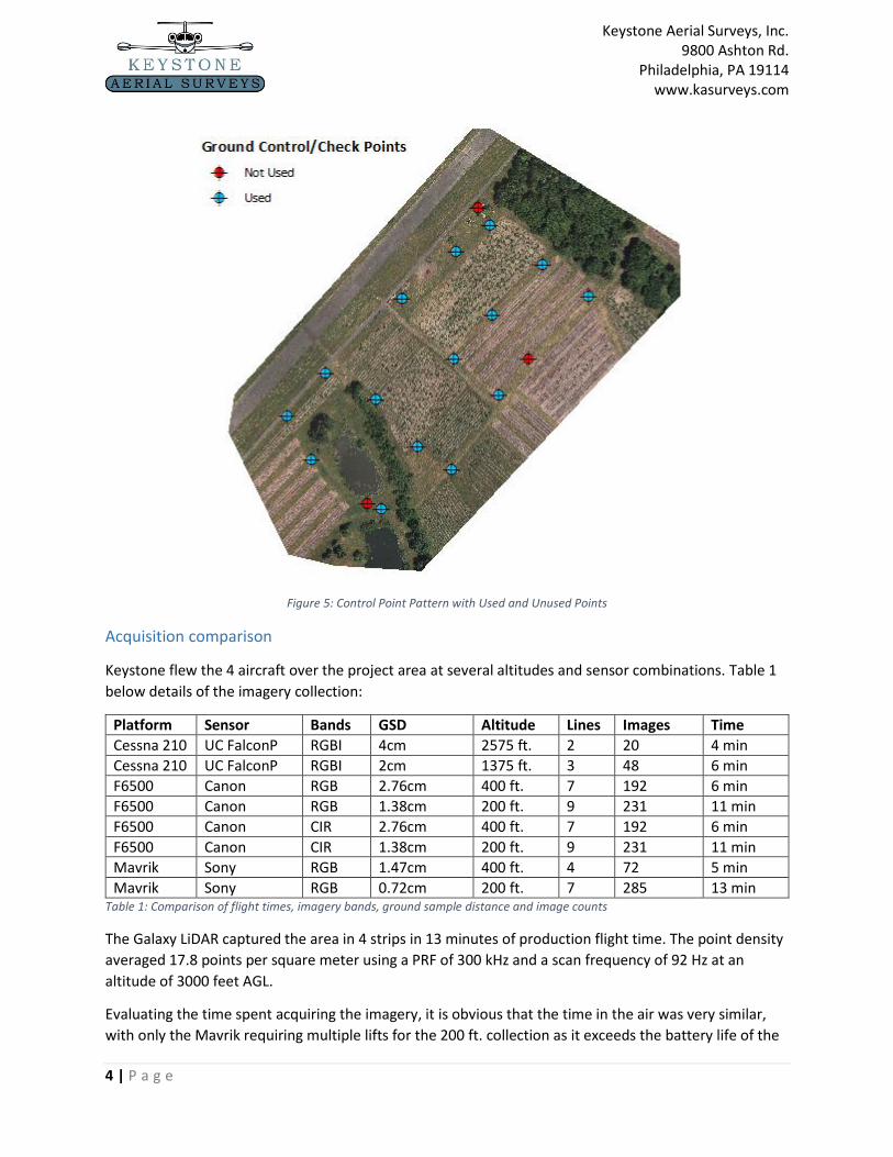
Control Layout

Before the flight day was scheduled, a team from Keystone

placed 18 control points throughout the test area in a

regular pattern. These were aluminum strips arranged in an

X pattern and painted white with a ground station GPS unit

used to record each location. The locations were processed

via the Online Positioning User Service (OPUS) to within an

accuracy of <3 cm. Keystone does not perform land survey

work as part of its business and so repurposed its base

station equipment for the task in order to minimize the

already substantial cost of this operation.

After using the control within the project, it was

determined that 3 points were incorrect and they were

removed from the solution, however this left Keystone with

1.4 control points per acre over the AOI. This excessive

control layout was designed to allow the processors to

experiment with varying amounts and location of control

while still having a significant amount left for check points.

Figure 3: SteadiDrone Mavrik X8 with Sony Camera

Figure 4: Control Point Installation and Measurement



4 | P a g e

Figure 5: Control Point Pattern with Used and Unused Points

Acquisition comparison

Keystone flew the 4 aircraft over the project area at several altitudes and sensor combinations. Table 1

below details of the imagery collection:

Platform Sensor Bands GSD Altitude Lines Images Time

Cessna 210 UC FalconP RGBI 4cm 2575 ft. 2 20 4 min

Cessna 210 UC FalconP RGBI 2cm 1375 ft. 3 48 6 min

F6500 Canon RGB 2.76cm 400 ft. 7 192 6 min

F6500 Canon RGB 1.38cm 200 ft. 9 231 11 min

F6500 Canon CIR 2.76cm 400 ft. 7 192 6 min

F6500 Canon CIR 1.38cm 200 ft. 9 231 11 min

Mavrik Sony RGB 1.47cm 400 ft. 4 72 5 min

Mavrik Sony RGB 0.72cm 200 ft. 7 285 13 min Table 1: Comparison of flight times, imagery bands, ground sample distance and image counts

The Galaxy LiDAR captured the area in 4 strips in 13 minutes of production flight time. The point density

averaged 17.8 points per square meter using a PRF of 300 kHz and a scan frequency of 92 Hz at an

altitude of 3000 feet AGL.

Evaluating the time spent acquiring the imagery, it is obvious that the time in the air was very similar,

with only the Mavrik requiring multiple lifts for the 200 ft. collection as it exceeds the battery life of the



5 | P a g e

aircraft. The total time required for a production flight for the manned aircraft would include time in

preparation and post flight for two crew members, but very little time on station. The total time for the

manned operation would be approximately 2 hours using 40 minutes for flight and 40 minutes of

preparation on either side of the flight. For the UAS, due to time spent in transit and setup on site, the

operation to collect just one type of imagery at one altitude would be 3.3 hours for one pilot.

The cost comparison of the two products is something that should be evaluated at this stage as well.

Assuming that the products produced are of similar quality, would the costs be similar or is the UAS

more cost effective? In the situation described here, the costs of acquisition for a manned aircraft

would likely be approximately $1300, while the UAS would be in the $600 range. However, if the project

where just 2 hours more driving from Keystone’s office, the price of the manned aircraft flight would

increase slightly, while the UAS costs could double (if an overnight stay is involved). More importantly, if

the project where in the same location but covered a large 1000-acre property, the UAS could need

multiple days to acquire the site to allow for movement to better visual viewing locations and battery

replenishment, yet the manned aircraft would be able to accomplish the task in just a few hours. The

costs of the manned aircraft are similar or less than UAS in this scenario and would provide far less

imagery to process.

Aerial Triangulation (AT)

Keystone used Pix4dmapper Pro for the initial UAS imagery processing. The UAS workflow in Mapper

Pro consists of importing the images and the navigation information from either the Exif data embedded

in the image or from an external file. At this point a rapid processing is done to tie the images together

in relative space. All points to be used are then measured and set as either control or check points and a

full AT is performed. After checking the results and making adjustments as needed, a full point cloud and

other deliverables are made. For the purpose of comparison to the Falcon imagery, projects using

various control point amounts were run: 2 control with 13 check, 3 control with 12 check and 5 control

with 10 check.

Detailed in table 2 below are some of the quality reporting elements from the point matching, bundle

adjustment and camera calibration performed by Pix4D for the UAS flights under various altitudes and

control patterns. Of interest is the camera optimization field, which is the percentage of change of the

lens focal length calculated and used by the software in order to optimize the solution. As can be seen

by the amount of adjustments made to the focal length, the Principal Point x and Principal Point y,

although the percentages remain small and within parameters, the values themselves vary. The amount

of change for the Sony is smaller, but varied while the Canon has a larger but more stable parameter

adjustment. This is likely due to lens factors such as stability, heat and vibrations. The average amount

of 3D points generated per image is very consistent between GCP configurations, but varies based on

sensor and altitude.



6 | P a g e

Camera Altitude GCPs Camera Optimization

Focal Shift (mm)

PP X shift (mm)

PP Y shift (mm)

Average 3D points per image

Canon 200 2 4.86% 0.973 0.012 0.121 5518

Canon 200 3 4.85% 0.971 0.013 0.122 5551

Canon 200 5 4.83% 0.968 0.012 0.123 5531

Canon 400 2 4.82% 0.964 0.005 0.139 10620

Canon 400 3 4.81% 0.960 0.006 0.141 10588

Canon 400 5 4.78% 0.957 0.005 0.141 10626

Sony 200 2 3.48% 0.626 -0.019 -0.066 9786

Sony 200 3 3.21% 0.546 -0.007 -0.073 9786

Sony 200 5 3.29% 0.579 -0.011 -0.068 9784

Sony 400 2 0.29% -0.104 -0.098 0.029 12214

Sony 400 3 0.38% -0.136 -0.071 0.400 13082

Sony 400 5 0.06% -0.022 -0.081 -0.001 12211 Table 2: Automatic camera calibration results for UAS datasets in Pix4Dmapper Pro

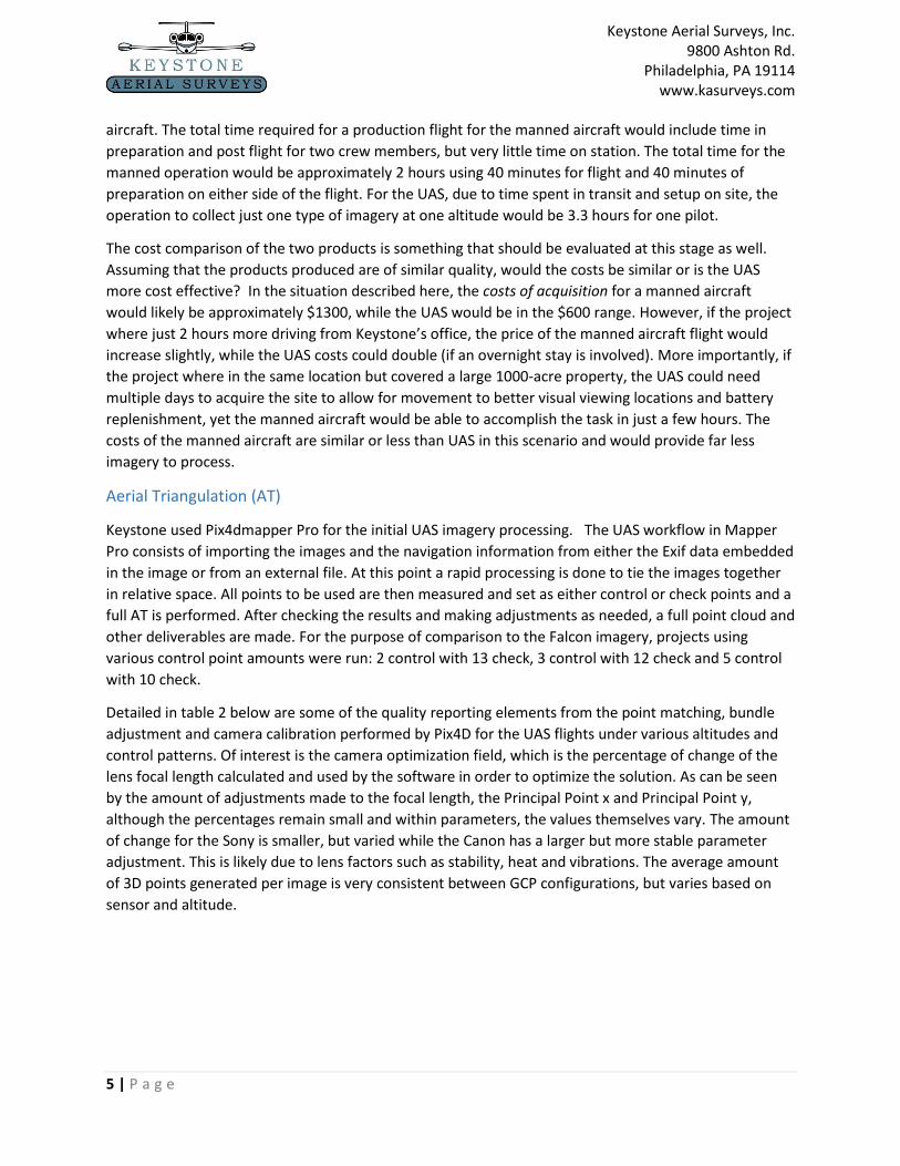
For the large format camera imagery, a standard Photogrammetric workflow using the INPHO suite and

the same control\check patterns were implemented. Below, in Table 3, is a comparison of the AT results

from the UAS mounted cameras with the results from the UltraCam Falcon and how they relate to

ASPRS accuracy standards. It is evident that the Sony performs poorly in Z at the lower altitudes with

limited control while the large format sensor performs best at all altitudes. However, Figure 7 highlights

that all of the UAS sensors generate 7cm or better vertical classification in the ASPRS accuracy

specification making the data acceptable for creating 1 foot contours, with the Sony producing height

and XY accuracies comparable to the UltraCam Falcon.

DX in cm DY in cm DZ in cm

Flight 2GCP RMSE

3GCP RMSE

5GCP RMSE

2GCP RMSE

3GCP RMSE

5GCP RMSE

2GCP RMSE

3GCP RMSE

5GCP RMSE

Sony 200ft 5.141 2.722 2.695 3.199 2.031 2.302 37.619 20.686 3.939

Sony 400ft 2.555 1.866 1.398 2.848 1.449 1.532 19.233 21.539 6.116

Canon 200ft 4.875 3.211 2.739 4.726 4.456 2.916 21.369 20.770 6.995

Canon 400ft 3.021 1.825 1.283 1.323 0.857 1.351 10.011 12.296 5.314

UCFp 1387ft 1.900 1.668 1.000 1.700 1.400 0.700 4.100 2.700 2.900

UCFp 2560ft 2.200 1.200 1.200 2.000 2.100 1.300 3.800 3.700 3.500 Table 3: Comparison of RMSE of AT of UAS Datasets



7 | P a g e

Figure 6: RMSE expressed in pixel size

Figure 7: RMSE expressed in ASPRS accuracy standards

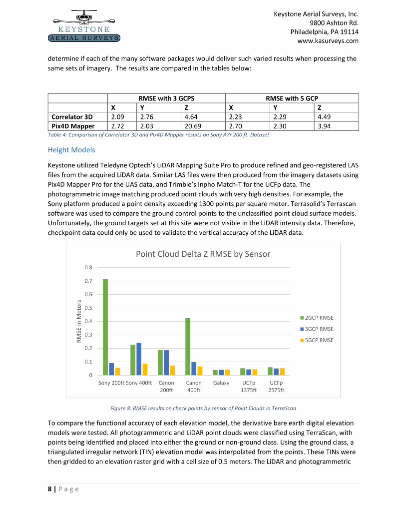
Due to the poor results in RMSE from the height measurements from the Sony and Altavian tests at 200

ft. with only 2 or 3 GCPs, Keystone used another software package to determine if better results could

be achieved. Simactive Correlator 3D was used to process the Sony A7r imagery with 3 and 5 GCPs.

The result for the 3 GCP test was vastly superior and produced a solid solution. However, the result

from the 5 GCPS test demonstrated only slight improvement and the RMSE in Z was actually inferior to

the Mapper Pro residuals. This clearly shows the differences in the algorithms of these two packages

create different results with the same GCP and image combinations. Further study should be made to

0

1

2

3

4

5

6

Sony 200ft Sony 400ft Canon 200ft Canon 400ft UCFp 1387ft UCFp 2560ft

RMSE Using 5 GCPs Expressed in Pixels

DX DY DZ

0.0

1.0

2.0

3.0

4.0

5.0

6.0

7.0

8.0

Sony 200ft Sony 400ft Canon 200ft Canon 400ft UCFp 1387ft UCFp 2560ft

ASPRS Accuracy Classification for Sets Using 5 GCPs

RMSEr RMSEz



8 | P a g e

determine if each of the many software packages would deliver such varied results when processing the

same sets of imagery. The results are compared in the tables below:

RMSE with 3 GCPS RMSE with 5 GCP

X Y Z X Y Z

Correlator 3D 2.09 2.76 4.64 2.23 2.29 4.49

Pix4D Mapper 2.72 2.03 20.69 2.70 2.30 3.94 Table 4: Comparison of Correlator 3D and Pix4D Mapper results on Sony A7r 200 ft. Dataset

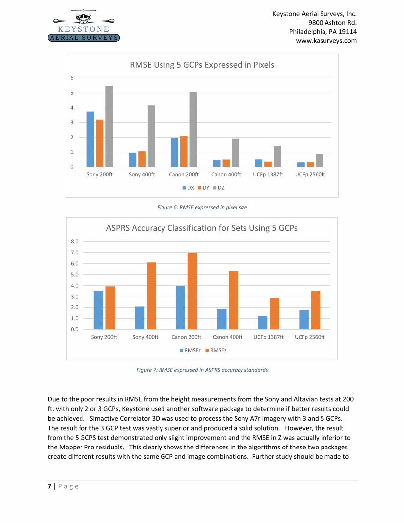
Height Models

Keystone utilized Teledyne Optech’s LiDAR Mapping Suite Pro to produce refined and geo-registered LAS

files from the acquired LiDAR data. Similar LAS files were then produced from the imagery datasets using

Pix4D Mapper Pro for the UAS data, and Trimble’s Inpho Match-T for the UCFp data. The

photogrammetric image matching produced point clouds with very high densities. For example, the

Sony platform produced a point density exceeding 1300 points per square meter. Terrasolid’s Terrascan

software was used to compare the ground control points to the unclassified point cloud surface models.

Unfortunately, the ground targets set at this site were not visible in the LiDAR intensity data. Therefore,

checkpoint data could only be used to validate the vertical accuracy of the LiDAR data.

Figure 8: RMSE results on check points by sensor of Point Clouds in TerraScan

To compare the functional accuracy of each elevation model, the derivative bare earth digital elevation

models were tested. All photogrammetric and LiDAR point clouds were classified using TerraScan, with

points being identified and placed into either the ground or non-ground class. Using the ground class, a

triangulated irregular network (TIN) elevation model was interpolated from the points. These TINs were

then gridded to an elevation raster grid with a cell size of 0.5 meters. The LiDAR and photogrammetric

0

0.1

0.2

0.3

0.4

0.5

0.6

0.7

0.8

Sony 200ft Sony 400ft Canon200ft

Canon400ft

Galaxy UCFp1375ft

UCFp2575ft

RM

SE in

Met

ers

Point Cloud Delta Z RMSE by Sensor

2GCP RMSE

3GCP RMSE

5GCP RMSE



9 | P a g e

DEMs were then compared to the checkpoints using QT Modeler. Results from the DEM are in Figure 9

below and point cloud control reporting can be seen in Figure 8 above.

Figure 9:RMSE results on check points by sensor of DEM in QT Modeler

In order to visualize the relative deviations between the models and the above error, it was decided to

compare the photogrammetric bare earth models to the LiDAR bare earth classification. This decision

was made for a number of reasons, notably because LiDAR is considered an industry standard in

elevation modeling and in this testing the LiDAR data consistently showed accurate results in Z when

compared to the check points. For testing and visualization purposes, a custom Python script using

ArcGIS 10.4’s ArcPy library was written to procedurally subtract each photogrammetric DEM from the

LiDAR DEM. The results of this calculation is a difference grid showing the deviation between the model

and the LiDAR model. These visualizations allow the analyst to see where high deviations are spatially

located throughout the project area. In these models, it should be noted that differences in the

classification removal of ground obstructions such as water, trees and shrubs have caused larger errors

to be evident in the southern end of the project area. This demonstrates a fundamental weakness of

photogrammetric models when compared to LiDAR: while LiDAR can “penetrate” tree canopy and

return some ground points, image matching generally cannot and must be interpolated across areas of

vegetation.

0

0.1

0.2

0.3

0.4

0.5

0.6

0.7

0.8

Sony 200ft Sony 400ft Canon200ft

Canon400ft

Galaxy UCFp1375ft

UCFp2575ft

RM

SE in

Met

ers

DEM Delta Z RMSE by Sensor

2GCP RMSE

3GCP RMSE

5GCP RMSE



10 | P a g e

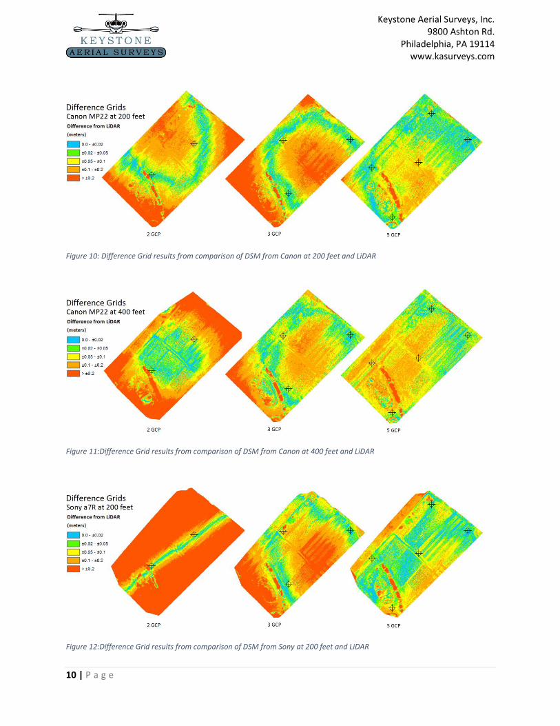
Figure 10: Difference Grid results from comparison of DSM from Canon at 200 feet and LiDAR

Figure 11:Difference Grid results from comparison of DSM from Canon at 400 feet and LiDAR

Figure 12:Difference Grid results from comparison of DSM from Sony at 200 feet and LiDAR



11 | P a g e

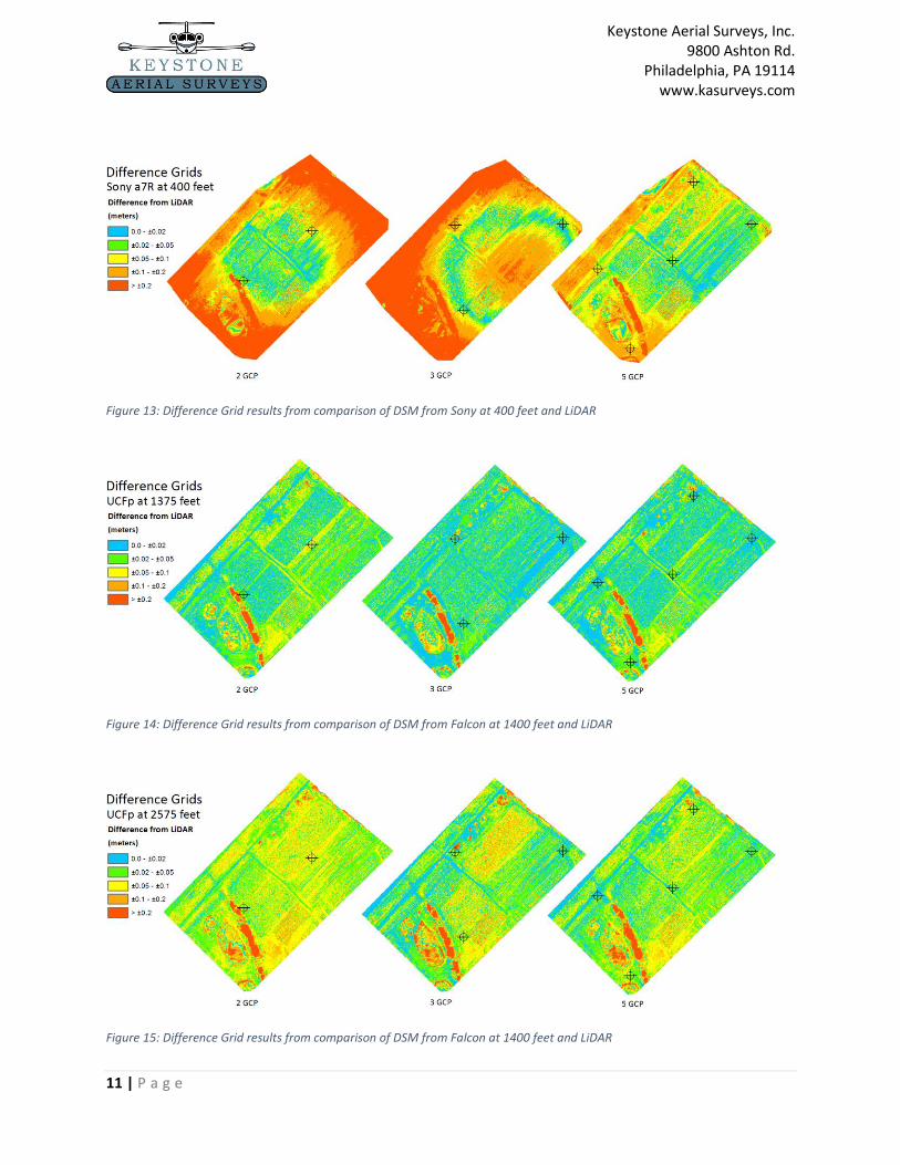
Figure 13: Difference Grid results from comparison of DSM from Sony at 400 feet and LiDAR

Figure 14: Difference Grid results from comparison of DSM from Falcon at 1400 feet and LiDAR

Figure 15: Difference Grid results from comparison of DSM from Falcon at 1400 feet and LiDAR



12 | P a g e

A number of conclusions can be drawn from these results. Perhaps most strikingly, the introduction of a

third ground control point dramatically increases the reliability of the results from the low altitude Sony

and the high altitude Canon when compared to the 2 GCP flight. This was reflected in the AT results and

the implications of these high residuals are apparent in the product. This is of no particular surprise;

neither the Mavrik nor Altavian platforms have high accuracy GPS/IMU sensors onboard, as is the case

with the UCFp and Galaxy LiDAR. While it was possible to use the telemetry data recorded during flight

to determine photo locations from the systems for each exposure center, these are not survey quality.

Two control points alone placed the model on a single axis about which it the model was rotated by the

algorithms in order to achieve the best results. This can be seen most obviously in the Sony 200ft 2 GCP

difference grid. The deviation is similar to the LiDAR only in a streak through the center of the project,

forming a line tracing the path of the ground control. The other ends of the project are either above or

below the actual terrain. The Canon 400ft flight had a similar but unique error pattern, with the center

of the model showing low deviation and the outside edges showing very high deviation. This could

indicate systematic errors present in the camera calibration, and the error could possibly be due to high

radial distortion causing warping of the model. More testing needs to be done here, but the issue

became less apparent as more control was added.

The addition of a third ground control point at minimum seems to be the best practice. However, five

ground control points consistently produced the best results with the UAS cameras. There was a small

increase in error (less than 2cm) when using 5 ground control points with the UCFp datasets. The team

attributed this to compounding error between the onboard GPS/IMU sensors and the existent error in

the ground control (<3 cm). Over a larger area or with higher accuracy ground control points, it is likely

that a result with a consistent RMSE of around 1 to 2 cm would be possible. It is interesting that while

the UltraCam Falcon Prime performed the best under all conditions, the smaller sensors were able to

nearly match the results when five ground control point are employed. The accuracies achieved here

may be more than suitable for a large number of applications, reinforcing the use of UAS and non-metric

cameras as a legitimate tool in many situations.

Normalized Difference Vegetation Index

One of the most common tools used in precision agriculture is the Normalized Difference Vegetation

Index (NDVI) which allows agronomists and growers to evaluate the health of many crops at all stages of

the growing season. In most use cases, strong absolute accuracy is not a necessity, since large areas of

extensive fields are targeted when applying fertilization, insecticides and other prescriptive measures

for a stressed crop. The index is created using the Near Infrared band (750-1040 nm) and visible red

band (620-750nm). The subtraction of the NIR from the visible divided by the addition of the NIR and

visible creates a pixel map with values between -1 and 1 for the entire image (Compton, 1979).

Keystone, using the CIR imagery collected from the Altavian mounted Canon MP22 camera, generated

an orthomosaic of the AOI. From the orthomosaic an NDVI map was created. The same procedure was

performed using the UltraCam Falcon 2cm GSD data with the results of a subset of the AOI is compared

below.



13 | P a g e

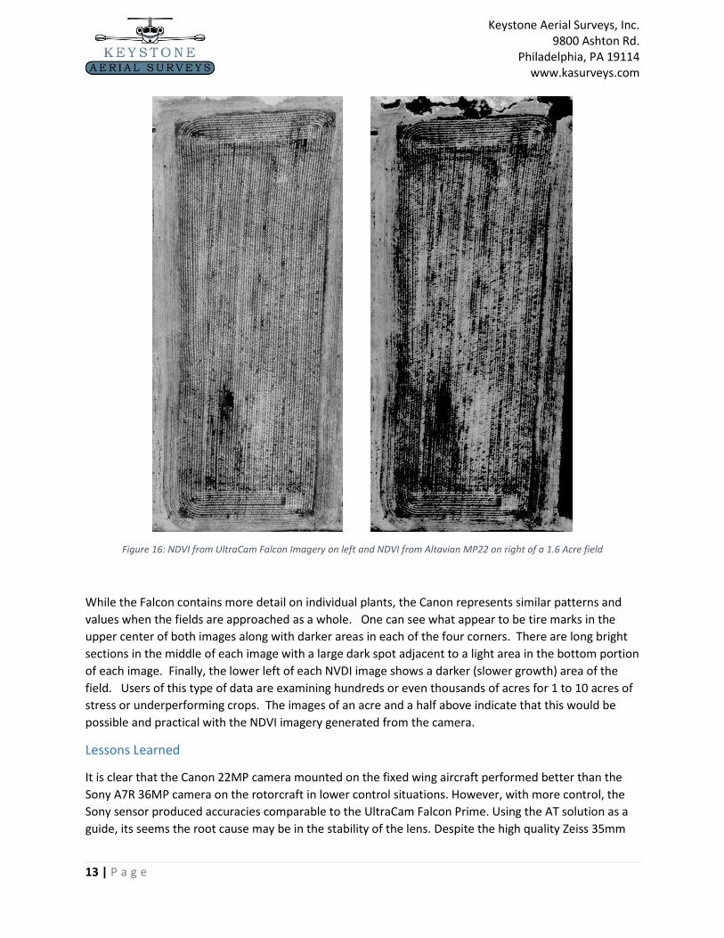
Figure 16: NDVI from UltraCam Falcon Imagery on left and NDVI from Altavian MP22 on right of a 1.6 Acre field

While the Falcon contains more detail on individual plants, the Canon represents similar patterns and

values when the fields are approached as a whole. One can see what appear to be tire marks in the

upper center of both images along with darker areas in each of the four corners. There are long bright

sections in the middle of each image with a large dark spot adjacent to a light area in the bottom portion

of each image. Finally, the lower left of each NVDI image shows a darker (slower growth) area of the

field. Users of this type of data are examining hundreds or even thousands of acres for 1 to 10 acres of

stress or underperforming crops. The images of an acre and a half above indicate that this would be

possible and practical with the NDVI imagery generated from the camera.

Lessons Learned

It is clear that the Canon 22MP camera mounted on the fixed wing aircraft performed better than the

Sony A7R 36MP camera on the rotorcraft in lower control situations. However, with more control, the

Sony sensor produced accuracies comparable to the UltraCam Falcon Prime. Using the AT solution as a

guide, its seems the root cause may be in the stability of the lens. Despite the high quality Zeiss 35mm



14 | P a g e

lens on the Sony A7R, the adjustments performed by the software would suggest an instability in the

lens, manifesting in poorer correlation, especially in Z. Whereas the Canon camera lens system has been

modified by the UAS manufacturer, resulting in a more stable lens system and more predictable results.

In the case of the Zeiss lens, the situation of less control caused the errors to manifest without the

ability to be systematically corrected.

In aerial triangulation, each camera performed better at the larger pixel sizes, especially the smaller

sensors, suggesting that the increase in the image amount compounded the level of tie point

uncertainty between control points and reduced the overall quality. It is also possible the very high

resolution images resulted in fewer obvious ground features and more image uniformity, resulting in

more false-positive tie points. While this was the case in triangulation, the higher resolution imagery

resulted in better residuals in Z when comparing the check points to both bare earth and surface model

products. This suggests a consideration of the end product must be undertaken before a survey is

conducted. The user must weigh the advantages of a higher relative AT accuracy with lower resolution

data versus higher resolution, rich imagery and high absolute accuracy in Z. This will largely be decided

by the final data application.

Continued development

Keystone is actively integrating and testing IMU and GPS/GNSS solutions that could further reduce the

number of GCPs necessary in all but the highest accuracy requirement products. The use of high quality

GNSS has greatly changed the landscape of traditional photogrammetry from large format cameras and

will most certainly do the same for UAS imagery. Adding the high frequency data collection of an IMU to

the solution will further the algorithms possible in post-production and in the bundle adjustment\self-

calibration routines.

Summary

Keystone found that with the proper control of a UAS solution a quality product can be generated for

almost any solution. Despite pricing considerations and the effects of many more images per acre, the

UAS imagery solution seems to be a viable solution in many circumstances. This is especially true when

tools that will reduce the reliance on GCPs become available and mapping sensors are purpose built for

UAS imagery capture.



15 | P a g e

Works Cited Compton, TJ. (1979). Red and photographic infrared linear combinations for monitoring vegetation.

Remote sensing of Environment, 8(2), 127-150. Retrieved from

http://ntrs.nasa.gov/archive/nasa/casi.ntrs.nasa.gov/19780024582.pdf

Federal Aviation Administration. (2016). FAA Aerospace Forecast: Fiscal Years 2016-2036. FAA. Retrieved

from http://www.faa.gov/data_research/aviation/aerospace_forecasts/

McCarthy, N. (2015, 10 19). Forbes Business. Retrieved from Forbes:

http://www.forbes.com/sites/niallmccarthy/2015/10/19/the-commercial-drone-sector-is-set-

to-contribute-billions-to-the-u-s-economy-infographic/#667016b47505

Shen, L. (2016, 5 25). Drone Sales Have Tripled in the Last Year. Retrieved from Fortune:

http://fortune.com/2016/05/25/drones-ndp-revenue/

uas imagery for high accuracy - kasurveys.com · uas imagery for high accuracy ... that the...

Documents