energy partition in the large-scale ocean circulation and...

Deep-Sea Research, 1974, Vol. 21, pp. 499 to 528. Pergmnon Press. Printed in Great Britain.

Energy partition in the large-scale ocean circulation and the production of mid-ocean eddies

A. E. GILL,* J. S. A. GREEN t and A. J. SIMMONS~

(Received 14 June 1973; in revised form 8 November 1973; accepted 8 November 1973)

Abstract--It is shown that the available potential energy in the large-scale mean ocean circulation, excluding the boundary layers, is of order ( BI a) s times the kinetic energy, where B is the basin dimension and a == c / f is the internal radius of deformation (c is the speed oflong internal waves andfthe Corinlis parameter). This ratio is of order 1000. The Sverdrup solution for a two-layer ocean is examined, and the rate of input of energy by the wind estimated. In the steady-state model, this energy is lost to the western boundary layer. It is then shown that potential energy available in the mean circulation can be converted into eddy energy by baroclinic instability. The stability properties depend only on the mean density field, and calculations are made for a number of cases. Maximum growth rates are obtained for eddies with wavelength of about 200 kin, typical e-folding times being about 80 days. These eddies have sj~,nificant velocities only in the surface layers. Secondary maxima in the growth rate curves are found for eddies with wavelengths of 300-500 km, e-folding times being 120 days or more. These eddies have sit, nificant velocities in deep water, their structure being something like that of the first baroclinlc mode.

In the models examined, the conversion of available potential energy took place in the upper 400 m, and the rate of conversion can be related to the maximum eddy velocity. If it is supposed that eddies grow to such a size that mean energy is lust to eddies as fast as it is supplied by the large-scale wind field, then the larger eddies would have maximum velocities of about 0.08 m s -1 and the smaller surface trapped eddies would have maximum velocities of about 0.14 m s-L Observations indicate the existence of eddies of this strength, and with wavelength and periods of the same order as given by the baroclinic instability calculations.

1. INTRODUCTION

OVER THE past century, a picture of the mean circulation of the ocean has been built up from temperature and salinity measurements (DEFA~r, 1961). The mean currents (see Fig. I) are only a few centimeters per second except in special regions of con- centrated currents like the Gulf Stream. However, direct measurements of currents have shown that the kinetic energy in time-dependent currents is greater than the kinetic energy of the mean currents and that currents of 0-I m s - I are commonly observed. The first direct current measurements over a long period (14 months) in mid-ocean were made in 1959 and 1960 in a region 5000 m deep about 250 km west of Bermuda. These measurements have been reported and discussed by CREASE (1962) and SWALLOW (1971). It appears that the eddies observed have wavelengths (PHILLIPS, 1966) of 300--400 km and periods (SWALLOW, 1971) of 50--100 days.

The U.S.S.R. POLYGON experiment (BR~HOVSKIKH, F~]n~OV, FOMIN, KOSHLYAKOV and YAMPOLSKY, 1971) has documented the progress of such an eddy in great detail. Observations were made using an array of current meters spread over a 200-kin square. The measurements indicate (KOSHLYAKOV and GRACHEV, 1973) that an eddy of elliptic shape (semi-axes 200 and 90 km) moved through the array at

*Department of Applied Mathematics and Theoretical Physics, University of Cambridge, Silver Street, Cambridge CB3 9EW, England.

tDepartment of Meteorology, Imperial College, London, England. ~Depertment of Geophysics, University of Reading, Reading, England.

499

500 A.E. GILL, J. S. A. GREEN and A. J. SIMMONS

0.04-0.06 m s -1. To give an impression of the scale involved, an ellipse of these d imensions is d rawn in Fig. 1 at the site of the P O L Y G O N experiment . This cor responds to a wavelength of about 360 km and a per iod of abou t 120 days. F igure 2 shows a progressive vector d iagram of currents a t 1000 m dur ing the experiment . Clearly, the current at any given t ime is little related to the long- term mean. Compare , for instance, the 10-day mean currents for the per iods 20th-30th Apr i l and the 20th-30th June. In both per iods the mean current was over 0.1 m s -1 but the direct ions were

=)(jo )OC" 9C ~' 8 0 " 70 " 6 0 " 5 0 * 4 0 ° 3~ ° 2 0 ) @ C @ K~* 2C P 3 0 " 4 0 " 5 0 °

(la)

Fig. I. Mean dynamic topography in the Atlantic Ocean (from DEFANT, 1961, Figs. 271,272) for (a) the ocean surface and (b) the 100=db surface. Contours are in dynamic crn. An ellipse with the dimensions of the eddy observed in the POLYGON experiment has been supcrimposeA in the

appropriate position.

coo. ~0 e 4 0 ' ~o • 2 o • I ~ W o - 10-o

Energy partition in the large-scale ocean circulation and the production of mid-ocean eddies 501

Eo-

oe

N

o, S

~ - ~ - ~ - z o , io - w o" i o - o

( l b )

totally different. On the other hand, the average current over the whole 6-month period of the experiment was similar to that deduced by Defant from temperature and salinity data.

An impression of how the eddies may be distributed in the horizontal at a particular time comes from measurements (Fig. 3) of sound velocity at 800 m made by BECKERLE (1972) (see also BECKERLE and La CASCE, 1973). The sound velocity is related to density so the contours indicate vertical shear. The arrows indicate the direction of motion for the layers above 800 m relative to those below.

I000 m

• ,o.v ~ '~_v

~,lV ~ IO.IV N

"v'I I ~ -30 .V I S

50 CM/SEC

30.VII.~20.VIt

Fig. 2. A progressive vector diagram of currents at 1000 m obtained in the POLYGON experiment (from BREKHOVSrdKH, FEDEROV, FOMIN, KOSHLYAKOV and YAMI'OLSKY, 1971, Fig. 4).

502 A.E. GILL, J. S. A. GREEN and A. J. Sn~tMONS

35 ~

f/ ./

• l

~o ° : " . .. j - , ,d" ,,,:;,:, / • . ~. . . . . "~,~, ,

[

' ~ SOUND VELOCITY CONTOURS (reelers/see f " [)E PTH 8 0 0 meters

ATLANTIS I I - 2 2 JUNE-AUG 1966

.'" ~.~o ~

r494

80 ° 75 ° 70 ° 65 ° 60 °

Fig. 3. Contours of sound velocity of 800 m in the Sargasso Sea (from BECKERLE, 1972). The sound velocity field is related to the density field and hence current shear. The arrows show the

direction of this shear.

The large eddies also appear as 'noise' on closely spaced hydrographic sections like those shown in the Atlantic Ocean Atlas of FUGLIS~V_m (1960) (a section from this atlas is reproduced in Fig. 6 below). The time taken to make a section is short compared with the period of an eddy and the station spacing (typically 100 km) is just small enough to indicate the presence of eddies without adequately resolving them. On the other hand, SECKVL (1968) reports a series of measurements between l0 and 26°N in the Pacific with 50-kin spacing, and this does appear adequate to resolve the most energetic eddies. WYRTKI (1967) has calculated the structure function for the depth of various isothermal surfaces, and finds a peak value at 250 kin, corresponding to a wavelength of about 500 kin. The amplitude of the displacement is about 50 m, and the 17 months of record (see SECr~L, 1968, Fig. 6C) appears to cover about 3 periods.

Further evidence of the presence of these energetic eddies may be found in the long time-series of temperature records obtained by the Panulirus at a station near Bermuda. The low frequency spectrum of the temperature at different depths is given by WUNSCH (1972b) and reproduced in Fig. 4. Most of the temperature variance comes from periods between 40 and 200 days. A similar feature is seen in the spectrum of dynamic height relative to 1500 db (WUNSCH, 1972a, Fig. 19).

Given that such eddies exist, the question is raised about the source of their energy.


2° I .o

I'0

o.e,

¢=

Fig. 4.

from Wunsch (1972) Doys Hours

756 200 42 20 12"42

. . . "...'~

, i i , , , + , I , : L , , t , , l , + , , ~ , , + . ' , ~ ÷ + l ~ . ~ " k . . . ~ e ~ e a l - l l ' k ' l l l W , ~ ' l " l " 4 + + ~ ' ~

0 10- 4 iO-3 iO-2 iO-I iO o l

Frequency (CPH|

The temperature spectrum q~f) at a depth of 500-600 m at the Panulirus station near Bermuda (from WVNSCH, 1972b, Fig. 2b). The temperature variancef~,(f) is plotted as a function

of frequency f

We will examine the partition of energy in the main oceanic gyres and show that most of the energy is stored as potential energy. Further, there is sufficient energy available to produce eddies of the observed strength if the potential energy of the mean flow is converted into eddy energy. Conversion of energy can take place by baroclinic instability, and a model of this process is examined. For the examples considered, substantial transfer of energy is found to occur only in the top 400 m. The most unstable disturbances are confined to the surface layers and have wavelengths of 100-250 km and e-folding times of 80-100 days. Longer waves (wavelength 300-500 kin) are also unstable but with e-folding times of 120-200 days. These waves have vertical structure similar to that of the first baroclinic mode and their stability properties arc strongly affected by bottom topography. The unstable disturbances examined were found to travel westwards with propagation speeds close to the maximum mean velocity, i.e. 4-5 km days -1. This corresponds to periods of 25-60 days for the short waves and 60-100 days for the long waves.

2. E N E R G Y P A R T I T I O N IN T H E M A I N O C E A N I C G Y R E S

The purpose of this section is to show, for a simple two-layer model of the ocean, that the potential energy stored in the main ocean gyres exceeds the kinetic energy by the large factor (B/a) ~, where B is the horizontal scale of the gyre and a is the (internal) radius of deformation. This is, in fact, a rather general property of quasi-gvostrophic flows (see Appendix). For the main oceanic gyres, B is of order 1000 km while a (at mid latitudes) is of order 30 kin, so the potential energy is of order 1000 times the kinetic. In particular, as STOMMEL (1965, p. 148) remarks, 'there is an immense store of available potential energy in the deep warm-water mass in the Sargasso Sea, more than a thousand times the kinetic energy of all the currents in the North Atlantic'. This fact is of great importance when considering possible sources of energy for the energetic eddies referred to in the introduction.

504 A.E. GILL) J. S. A. GREEN and A. J. SIMMONS

To demonstrate the result, consider the case of geostrophic flow in a two-layer ocean, the lower layer of which is at rest (c.f. STOMMEL, 1965, Chapter 8). This gives a reasonable order-of-magnitude approximation to the wind-driven flow in the main oceanic gyres, since the main currents are confined to the upper part of the ocean. In this section, orders of magnitude of the potential and kinetic energy will be compared. In the next section, more specific calculations will be made for the 'Sverdrup' solution for an ocean gyre.

Let x, y, z be co-ordinates such that x increases eastwards, y northwards and z upwards, and let u, v, w be the corresponding velocity components. Suppose the ocean surface is defined by

= = , l ( x , y ) ,

and the interface between the upper fluid (of density pl) and the lower fluid (of density p2) is given by

z = --h(x ,y) .

Then if g is the gravitational acceleration, the hydrostatic relation gives for the pressure, p,

{ o l g ( ~ -- z) for --h < z < '/ p = (2.1)

p l g ( ~ + h ) - - p 2 g ( h + z ) f o r z < - /7 .

I f the lower layer is motionless, p must be constant on horizontal surfaces so

g~q = Fl(z) + g 'h ,

where

g ' = (p2 -- pl)g/Pz.

Therefore, the pressure in the upper layer is given by

p/p , = g'h + F2(z),

where FI and F2 are functions of z only. The velocities in the upper layer are given in terms of h through the geostrophic relation

-- fv = --Px/p1 = --g'hx (2.2)

f u - : --Py/ pI ~--- - -g 'hy,

except in a thin Ekman layer adjacent to the surface. The average kinetic and potential energy can now be estimated for a gyre with

east-west scale L and north-south scale B with B < L. The overbar will be used to define the average over the main part of the gyre, e.g.

h = I f h dx dy/I I dx dr,.

The integration is confined to the region where the variations are on the large scales L and B and excludes the region of strong boundary currents. The average kinetic energy, T, per unit area is given by

T : ½Plh(u 2 + v z) : ½plg'h(hx 2 + hv2)/f 2. (2.3)


The available potential energy, V, is defined as the change in potential energy obtained by flattening the interface. The average value 17 per unit area is given by

D = ½ptg'[h 2 - - (h)2]. (2.4)

Now let

h = h + h', (2.5)

where h' is assumed to be either small compared with h or else the same order of magnitude. It follows that, in order of magnitude,

T ,.., plg'Zh h '2 /B~f 2 (2.6)

17 ~ rag' h'2. (2.7)

The ratio

where

~/T ,,, B~/a ~, (2.8)

a = ( g ' h ) t / f = c ' / f (2.9)

is the (internal) radius of deformation and c' the speed of long internal waves. Hence the result that the potential energy exceeds the kinetic energy by the factor (B/a) 2.

3. ENERGETICS OF SVERDRUP FLOW

(a) Es t ima te s o f the mean k ine t ic and mean po ten t ia l energy densit ies

Specific results are easily calculated for the wind-driven Sverdrup flow (see STOM~L, 1965, Chapters 7 and 11) in a two-layer ocean. Suppose the line x = 0 lies to the east of the western boundary region and the eastern boundary is at x = L. Suppose there is an eastward wind stress given by

sin ( y / B ) .

The divergence of the Ekman transport driven by this stress results in a vertical velocity,

W~.k -- --(r/fBpl) cos (y/B) (3.1)

just below the Ekman layer and this drives the geostrophic flow which satisfies (2.2). It has been assumed that B is small compared with the radius of the Earth. The flow can be calculated by using the continuity equation for the part of the upper layer which excludes the Ekman layer, namely

(hu)x + (hv)v + W~k = O. (3.2)

By eliminating u, v in favour o fh in (2.2) and (3.2) and using the condition of zero transport across x = L, there results

h 2 = ho 2 + ( 2 f i / p l g ' B f l ) (L - - x ) cos ( y / B ) , (3.3)

where h0 is a constant and fl = d f /dy . With the further assumption that h' ~ h, and hense that h' ~ h0, the mean energies

can be calculated. Averages will be taken over the region 0 < x < L and over one period

506 A.E. GILL, J. S. A. GIVEN and A. J. SIMMONS

in the y-direction. For small h', it follows from (3.3) that

h - ho + ( fr /mg'hoBfl) (L -- x) cos (y/B)

- [(fi'/plg'hoB/3) (L -- x) cos (y/B)]2/(2ho), (3.4)

and so

h ~ ho - [fTL/plg'hoB~]2](12ho). (3.5)

It follows that

and

17 : [f~.L/hoB~]2/(12 plg') , (3.6)

I ' ---: [r/B/3] 2 [(L 2 + 3B2)/B2]/(12plho). (3.7)

It will be observed that for L >> B,

~/7": (B/a)2. (3.8) For the following values in S.I. units; r : 0.1 N m - 2 , f - - 10 -4 s -1, p l : = 103 kg m -3, / 3 : 2 × 10 - l x m - i s - a , c ' = 3 m s - l ( g ' = 0 . 0 2 m s -2 ,h = 500m), B : 10 era , L = 5 × 10 e m, one obtains

h'max = 250 m, :r : 100 J m -2, I 7 .... 105 J m -2.

The value of 7' corresponds to mean currents in the upper layer of 0.02 m s -1.

(b) Rate o f input o f energy into the Sverdrup f low

Now that the partition of energy within the Sverdrup flow has been calculated, we go on to calculate the rates of input and output of energy. The relevant energy equation is obtained by multiplying the first of (2.2) by plhU, the second of (2.2) by plhv, equation (3.2) by plg'h and adding all three. The result is

0 : --plg'(uh2)~ -- pxg ' (vhZ)v - plg'hw~k.

Integrating over the region, this becomes

0 : plg'[Suh 2 dy]x= 0 -- pig' ~ hwEk dx dy. (3.9)

The second term represents the rate of input of energy into the Sverdrup flow by the working of pressure forces at the base of the Ekman layer, i.e. this is the rate of input of energy to the region below the Ekman layer which results from the action of the wind. This is balanced by the first term representing the output of energy which is lost to the western boundary region. The average rate, ~, of input can be calculated using (3.1) and (3.4), viz.

t~ : plg'hWEk -- T2L/4plhoB2/3 - 10 -3 Wm -2. (3.10)

A summary of the results is given schematically in Fig. 5. This number is important when we consider possible instabilities of the Sverdrup region, for instabilities imply transfer of some of the energy of the mean flow into eddy energy. Obviously, the rate of transfer of energy to eddies cannot be greater than the rate of supply of energy to the mean state by the wind.

The rate of energy input to the mean flow can be compared with the energy con- tained in the mean flow. The ratio

17/1~ -- L/3/3a z ~ 3 yr (3.11)


,Energy fed in by wind is of overoge rote R (NI0"SWm -2)

h

Fig. 5. A sketch showing the energy budget for the Sverdrup solution in a two-layer ocean in which the lower layer is at rest. The sketch shows the position of the interface, the energy transfer across the surface, the energy transfer to the western boundary current and energy stored. The expressions for R, Fand fare given in the text. The estimates are based on values given in the text.

is the time it would take to build up the mean flow at the mean rate of input if the energy of the mean flow were suddenly removed.

4. MAXIMUM POSSIBLE S T R E N G T H OF E D D I E S

Suppose now, that, by some mechanism as yet undefined, energy from the mean flow described above is converted into eddies. How strong can the eddies be ? Clearly, there is little kinetic energy available for the eddies to draw on, but there is a considerable store of potential energy. To find the maximum possible average strength of eddies, we can calculate the average energy, P-~day, if all the energy in the mean flow were converted into eddies. In this case

~eddy = /7, (4.1)

i.e. the average eddy energy equals the average available energy. Let the wave number of the eddy be k. I f k -1 is greater than the radius of deformation, then the eddy energy is mostly potential energy, Fedd~, so

/Teddy -~- ff--addF = /7. (4.2)

The average kinetic energy, Teddy, is less by a factor (ka) 2, so

~eddF = (ka)~ /7 = (kB) z •. (4.3)

Thus the eddy kinetic energy can be much larger than the mean kinetic energy if their scale is less than that of the mean flow. For instance, if k-1 = 100 km and B = 1000 kin,

508 A . E . GILL, J. S. A. GREEN and A. J. SIMMONS

the eddy kinetic energy could be 100 times bigger, viz. 0-2 m s - t compared with 0.02 m s -1 for the mean flow.

A pictorial interpretation of this result can be given in terms of the two-layer model in which the average potential energy is proportional to the mean square displacement of the interface whereas the average kinetic energy is proportional to the mean square slope of the interface. For the mean flow the interface has a small slope because the scale is large. If the potential energy of the mean flow is converted into eddies, the mean square displacement of the interface is unchanged but the mean square slope is greatly increased if the scale of the eddies is small compared with the scale of the mean flow.

An impression of how much energy is in the larger eddies and how much is in the mean flow can be obtained from examining oceanographic sections. For instance, the temperature section at 50°W (Fig. 6) from FUGLISTER (1960) shows that the thermocline (8-16°C) between 25 and 35°N slopes down to the north, dropping about 140 m in this distance. (Between 15 and 35°N, the same isotherms descend about 400 m.) The wiggles on these isotherms represent displacements of ±25 m, i.e. the displacements due to eddies are rather less than the displacements in the mean flow. This indicates that the

potential energy (which is proportional to h '2) of the eddies is 15-20 ".,~ of that available in the mean flow over the 10 ° interval (25-35°N), and a much smaller fraction (a few per cent) of the energy available over the 20 ° interval.

I f the thermocline slopes from north to south, the baroclinic eddies can extract most energy when they have a large north-south scale and the proportion of this which is kinetic energy is largest when they have a small east-west scale. The impression from the Fuglister section is that the eddies have the energy obtainable by extracting that available in a north-south distance of order 500 km.

5. C O N V E R S I O N OF A V A I L A B L E E N E R G Y TO E D D Y E N E R G Y

Although there is a vast store of potential energy available in the mean circulation of the ocean, it is not obvious that this can easily be drawn on to form eddies. In fact, the constraints imposed by the rotation of the Earth make the energy conversion rather difficult. However, the analyses of CrtARNEY (1947) and EADY (1949) have shown that this energy conversion can take place in the atmosphere. G~EN (1970) has shown that the observed structure of atmospheric eddies, as represented by their transfer properties, is consistent with perturbation theory. Moreover, the eddy intensity and the magnitude of the transfer is consistent with the conversion of available potential energy into eddy kinetic energy. SCHULMAN (1967) has made calculations for an ocean circulation with a rather weak thermocline and found unstable eddies with an e-folding time of about a year, but he felt that stronger growth would occur with a more realistic mean circulation. The remainder of this paper will be devoted to examining the stability of different mean flow profiles. The results are quite sensitive to the profiles taken, and for that reason a variety of profiles will be considered.

We consider small disturbances to a mean state in which the density p varies with both depth and horizontal position. The horizontal scale, k -1, of the perturbation is assumed to be small compared with the horizontal scale of the density variations, so that locally the perturbation can be considered to be a superposition of plane wave solutions, and the only properties of the mean field on which the solution depends are the variations of # and of its horizontal gradient with depth. The perturbed motion is

Fig. 6. The meridional temperature section at 5O”W, from FUGLISTER (1960).

[facing p. SOS1


assumed to be quasi-geostrophic and hydrostatic, in which case (see, for example, GREEN, 1960, or CHARNEY and STERN, 1962) a disturbance stream function ~ can be introduced, which, for a plane wave, has the form

~(x , z , t ) = R e { ¢ ( z ) e ~ ( z -e t ) }, (5.1)

the x-axis being chosen to be in the direction of phase propagation. The perturbation pressure, p, the perturbation density, a, and the perturbation velocity components, u, v, w are given in terms of ~k by

p - - - po f¢

U ~ - - ~ b y

v = ~ z (5.2)

g a = - - po f~b z

NZw = --f(~bzt + OCzz- Oz~bx),

where p0 is a representative value of the density and the equation satisfied by the complex amplitude, ¢, of the stream function is

( U - - c) {[ ( fZ /NZ) $dz -- kZ¢} + Qua/' = 0, (5.3) where

Qv = j8 - - [ ( f2 /N~) Oz]:. (5.4)

In the above equation, O is the component of the current in the x-direction and so is related to the y-derivative of p by the equation

f U z = gPv/Po. (5.5)

Also, the function N ( z ) which appears in the equations is the Brunt-Viiisiilii frequency, defined by

N ~ = - -gpz /po , (5.6)

and fl is the y-component of the gradient o f f Since the mean density gradients in the ocean are mainly in the north-south direction, the disturbances which can most easily draw on the potential energy available are those which travel in the east-west direction. Therefore, in the examples, the x-axis is normally chosen as pointing eastwards, in which case fl has its usual meaning.

The boundary conditions are those of no normal flow. At the surface z = 0, this condition is w = 0, which in terms of ¢, gives

$z/¢ = Oz l (O - - c) at z = 0. (5.7)

The boundary condition at the bottom z = - - H is

$z/¢ = (Oz + N ~ H y / f ) [ ( O - - c) at z = - -H. (5.8)

For given wavenumber, k, the equations and boundary conditions define an eigenvalue problem for c. A complex c with positive imaginary part implies the existence of a mode which grows with time, and the flow U(z) is then said to be baroclinically unstable. For the case of a flat bottom (Hv = 0), necessary conditions for instability are (GREEN, 1960; CBARNEY and Slw_.RN, 1962) that either

(i) Qv change sign in - - H < z < 0,

510 A.E. GILL, J. S. A. GRI~N and A. J. SIMMONS

or (ii) the sign of Qu be opposite to that of Oz at z = 0, or (iii) the sign of Qv be the same as that of 0z at z = -- H. A trivial modification of the argument shows that, for the general case, the last condition should be

(iii) the sign of Qv be the same as that of 0z + N2Hy]fat z = - H . The above conditions can be exploited to show that some profiles are stable. When the necessary conditions are satisfied, however, a detailed stability analysis is required to show if the flow is in fact unstable, and, when it is, to find the growth rates, etc.

From the way the positive quantity N ~ appears in (5.3), it can be seen that minor details in the form of the profile N2(z) are not critical. In the calculations reported here, the profile

NZlf ~ = 10 4 e z/a (5.9)

has been used, with d = 900 m. This should model the reduction of N 2 with depth in the deep layers reasonably well. The effect of a reduction of N 2 near the surface was calculated for one ease only, and the results are given later.

The values ~ = 2 × 10 -11 m -1 s -x and H = 4500 m have been used throughout. The critical profile for stability considerations is that of Qy (which depends on Oz) and so is [see (ii) above] the sign of Oz at the surface. Now Oz is proportional [see (5.5)] to the horizontal density gradient, so a major factor affecting stability is the way in which the horizontal density gradient varies with depth. In fact, substituting (5.5) and (5.6) in (5.4),

Qv = [3 + f(Pu/Pz)z, (5.10)

and depends on the slope Pv[#z oftbe isopycnals. It will be found that when this slope is uniform, only westward currents are unstable, which corresponds to having denser water toward the equator. However, at the surface, the denser water is normally toward the poles, so the slope of the isopycnals can reverse near the surface (see Fig. 6).

In order to examine the effects of such a reversal, we will examine the stability of the profiles shown in Fig. 7. In all cases, the maximum velocity is 0.05 m s -1 Profile [1] has the same exponential form as in (5.9), namely

O(z) = UoeJ a, (5.11)

with U0 = --0-05 m s -t. This corresponds to a uniform slope of the isopycnals. The value of the slope depends on f , and is 0.8 × 10 -a at 30 ° and 1-1 × 10 -a at 20 ° latitude. These values are about 60 ~o of the maximum values observed in the section shown in Fig. 6.

The other profiles shown in Fig. 7 are given by

U(z) = Uo ~la _ U1 ~la. (5.12)

The maximum velocity of Um,x ----- -0"05 m s -1 is achieved at a depth z = --zraax, and so the profiles are completely specified by the choices of a and Zmax. a is 100 m for profiles [2], [3] and 400 m for profiles [4], [5]. Zmx is zero for profiles [2], [4] and 100 m for profiles [3], [5]. Thus, for profiles [2] and [4], the slope oftbe isopyenals becomes zero at the surface. For profile [2], the change in slope is rapid while for profile [4] it is slow. For profiles [3] and [5] the slope of the isopycnals reverses at 100 m. The change in slope is rapid for profile [3] and slow for profile [5].


(cms- '} I 2 3 4 5 4 5

I O I 2 3 ,4 5

Fig. 7. Mean velocity profiles O(z) for which a stability analysis has been carried out. For clarity, profiles [4] and [5] have been displaced to the right and profile [1] is drawn twice. Note that the scale of z is limited to less than half the total depth. The mean currents below 2000 m are very small.

The necessary condition for instability can now be applied. For profile [1], since the isopycnals have uniform slope

Q~ = ~, (5.13)

i.e. is independent ofz . Thus the necessary condition can only be satisfied if Oz has the appropriate sign at the boundaries. Oz is so small at the lower boundary that only a weak instability can occur when this has the appropriate sign. Otherwise, instability can only occur when U0 < 0 so that Oz has the opposite sign to Qv at the surface. This corresponds to a westward current with isopycnals sloping upwards towards the equator.

For the remaining profiles, Qy is close to ~ near the bottom and departs from/3 by increasing amounts as the surface is approached. The surface value is given by

Qy = f1-4- 10 -4 (Umax/ad) e z~'~la.

If Umax is negative (westward currents), Qy changes sign if

a e -zm*xl~ < --10 --4 Umx/~d ~- 278 m,

which does happen for the two profiles with a = 100 m but not for the profiles with a ---- 400 m. Thus profile [4] must be stable. Profile [5] could only be unstable if Um,x were positive (an eastward current) so that Oz at the surface would have the opposite sign to Qu. However, Oz has such a small value that [fan instability occurred it would be very weak. Thus the stability analysis is only carried out for profiles [1], [2] and [3] with westward flow.


It is important to note that the stability problem requires only a knowledge of the mean density field. This is because only velocities relative to a reference level appear in the equations and boundary conditions. If 0 is changed by a constant (i.e. an amount independent of depth), (5.3), (5.4), (5.7) and (5.8) show that the only effect is to change the wave speed Cr by the same amount. The growth rate is unaffected. It is, therefore, possible to use the density data available in data banks to divide the ocean into regions with different baroclinic stability properties e.g. categories such as 'stable', 'weakly unstable' and 'strongly unstable'. Perhaps experience with a relatively small number of mean profiles would allow a crude classification like this to be made. The necessary condition for instability would allow some areas to be classified as stable without detailed analysis. The results discussed in the next section show that the density structure in the top 400 m can strongly affect the stability, and so conditions can change seasonally. Since e-folding times are 3 months or more, it would be necessary to assess what the average effect over a whole year would be using the stability properties for each individual season.

6. STABILITY RESULTS FOR C O N T I N U O U S PROFILES

Numerical solutions were obtained for the profiles [1]-[3] by taking an initial guess for c which determines, by (5.7), the value of ~bz/~ at z = 0. Then (5.3) was inte- grated to find the value of ~z/~b at z ---- - - H and this was compared with the value given by (5.8). The exact value of c was subsequently obtained by iteration.

Figure 8 shows the growth rate, kc~, and wave speed, cr, as functions of k for the exponential profile [1]. cr and c~ are the real and imaginary parts of c. For the case of a flat bottom, the wave speed was found to vary only a little, with values ranging from 44-50 mm s-L This corresponds to a 'steering level', i.e. the level at which 0 equals cr, somewhere between the surface and a depth of 100 m. Results are shown for three different values of the non-dimensional bottom slope [see (5.8)]

s : ( N ~ / f ( l z ) ~ = _ n H v = (#z /~v)~=_nHv, (6.1)

namely s = - - 10, s = 0 and s = 10. s is negative when the bottom slopes the same way as the isopycnals. The value s = 10 corresponds to a bottom slope of 0.6 × 10 -a when f = 10-4 S-1.

For wavenumbers above 0.03 km -x, the stability characteristics are practically independent of s. The minimum e-folding time of 80 days is achieved for a wave length of 190 km. For smaller k, the growth rate curves all show a secondary maximum, but the value and position of this maximum are strongly dependent on s. For s -- 0, it occurs at a wavelength of 330 km, where the e-folding time is 120 days.

An indication of the way in which the value ofs affects stability comes from the third alternative of the necessary conditions for instability, namely that Qu has the same sign as Oz (1 + s). For profile [1], westward currents (Oz < 0) are destabilized only when s < -- 1, i.e. when the bottom slopes up towards the equator. This seems consistent with the result (Fig. 8) that the negative s case is the most unstable for small k. For eastward currents (Oz > 0), the necessary condition is satisfied when s > --1. Presumably the most favourable conditions for instability are obtained when s is large and positive. This also corresponds to the bottom sloping upwards towards the equator.


'4 S ~ 4

m 2

e- (3.

i I I I . , =

• o l 0 2 O3 0 4 "05 k(km"l)

~ ' 0 1 2 I0

~ ' 0 0 8

~'004

S=O - - - S=IO . . . . . s . - i o

/ I \I "(31 "02 "03 04 "05

Wovenumbcr k(km "I)

Fig. 8. Phase speed, c,, and growth rate, kc, as functions of wavenumber k for the exponential profile Ill. Values are shown for three values of the non-dimensional bottom slope s = 0 4- 10. s is

the bottom slope divided by the slope of the isopycnals at the bottom.

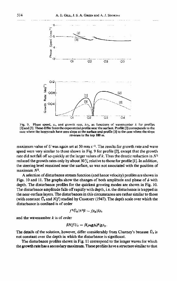
The wave speeds and growth rates for profiles [2] and [3] are shown in Fig. 9. The main feature is that the growth rates are generally smaller. Typical e-folding times are 30-40% larger for profile [2] than profile [1], while the e-folding times for profile [3] are typically double those for profile [1]. In other words, reducing the slope of the isopycnals near the surface reduces the growth rate, and reversal of the slope of the isopycnals at the surface reduces the growth rate still further. Thus changes in the conditions in the top 100 or 200 m can make large changes in the stability properties. Such changes do occur with the progression of the seasons (which h aw a time scale comparable with the e-folding time) so seasonal changes will have important effects on thegrowth of disturbances. The wave speeds again are close to the maximum velocity of 50 m m s -1 and can even be greater. PEDLOSKY (1964, p. 211) has shown that this is possible when the t-effect is important.

One further calculation was made in which N 2 was substantially reduced near the surface, so the maximum value was at 800 m. Below 800 m, N/fwas the same as for the other profiles, i.e. as given by (5.9). However, between 800 and 200 m, N/ f changed approximately linearly from 63 at 800 m to 35 at 200 m, and remained approximately constant at this value to the surface. This corresponds to a reduction o f N 9- at the surface by a factor of 8 relative to the other cases. The slope of the i sopycnals was kept constant, so Q~ - fl as for profile [1]. This implies a reduction of shear near the surface. The

514 A . E . GILL, J. S. A. G m N and A. J. SIMMONS

-6 F T

[21

[ '

m -4!

0. -3 [ . . . . . . . . . . . . . . . . . . . . . . . . . . . ~ - . . . . . . . . . . . . . . . . . . . . . . 01 0 2 0 3 03

012 l- . . . . . . . . . . . . . . . . . . . . . . . . . . . . . . .

0 i

t9 L.. 1- Ol 0 2 0 3 0 4

Fig. 9. Phase speed, Cr, and growth rate, kc,, as functions of wavenumber k for profiles [2] and [3]. These differ f rom the exponential profile near the surface. Profile [2] corresponds to the case where the isopyenals have zero slope at the surface and profile [3] to the case where the slope

rever~-'s in the top I00 m.

maximum value of U was again set at 50 mm s -1. The results for growth rate and wave speed were very similar to those shown in Fig. 9 for profile [2], except that the growth rate did not fall off so quickly at the larger values of k. Thus the drastic reduction in N z reduced the growth rates only by about 30 ~ relative to those for profile [1]. In addition, the steering level remained near the surface, so was not associated with the position of maximum N 2.

A selection of disturbance stream function (and hence velocity) profiles are shown in Figs. 10 and 1 I. The graphs show the changes of both amplitude and phase of ~ with depth. The disturbance profiles for the quickest growing modes are shown in Fig. 10. The disturbance amplitude falls off rapidly with depth, i.e. the disturbance is trapped in the near-surface layers. The disturbances in this circumstance are rather similar to those (with constant Oz and N/f) studied by CrL~NnY (1947). The depth scale over which the disturbance is confined is of order

fzOz/N2# = f#y/##z

and the wavenumber k is of order

[3N/fUz = [3(pogpz)t/g#y.

The details of the solution, however, differ considerably from Charney's because Oz is not constant over the depth in which the disturbance is significant.

The disturbance profiles shown in Fig. 11 correspond to the longer waves for which the growth rate has a secondary maximum. These profiles have a structure similar to that


Amplitude Phase

0 5 I 0 ° - 6 0 °

lO00m /

I500m ~

.- [ l ] , [2 ] , [3 ]

Fig. 10. Disturbance velocity profiles for the most rapidly growing disturbances, showing the amplitude and the phase. The amplitude is shown relative to its maximum value, and the phase relative to the value at the bottom. Only values for the top 2000 m are shown, as the amplitude is very small below this depth. The wavenumbers of th¢ disturbances are [1] 0.033 kra-l ,

[2] 0.0285 km -1 and [3] 0.0275 kra -1.

of the first baroclinic mode (which is the disturbance profile in the absence of shear). The amplitude has a minimum value at a depth of about 1000 kin, with a phase change of 180 ° between levels a few hundred meters above and below. Thus at any given time, the velocity profile shows a change in sign at depth of about 1000 kin. Because the amplitude of this disturbance is significant in deep water, the properties of the disturbance are significantly affected by bottom topography, as Fig. 8 demonstrates.

7. ESTIMATES OF THE ENERGY CONVERSION RATES AND BUOYANCY FLUXES

The previous calculations allow estimates to be made of the rates at which available potential energy is converted into eddy energy provided the amplitude of the eddies is known. This can then be compared with the estimate of Section 3 of the rate at which available potential energy is being created by the large-scale wind field. One can also calculate the north-south buoyancy flux produced by the eddies. Before doing this, an interesting fact emerges as to the sign of this transfer. Because of the effect of ~ on the stability, the most favourable conditions for instability are found where the isopycnals


lO00m

2000m

3000m

Ampl i tude Phase

0 . 5 I 0 ° - 9 0 ° -180 ° - 2 7 0 °

[2 Ils=_lo ,,, A [I] s - o

4000m

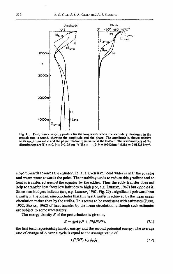
Fig. 11. Disturbance velocity profiles for the long waves where the secondary maximum in the growth rate is found, showing the amplitude and the phase. The amplitude is shown relative to its maximum value and the phase relative to its value at the bottom. The wavenambers of the disturbances are [1] s = 0, k = 0.0195 km -1 ; [1] s = -- 10, k = 0.012 krn -1 ; [2] k ---- 0.01825 km -1.

slope upwards towards the equator, i.e. at a given level, cold water is near the equator and warm water towards the poles. The instability tends to reduce this gradient and so heat is transferred toward the equator by the eddies. Thus the eddy transfer does not help to transfer heat f rom low latitudes to high (see, e.g. LORENZ, 1967) but opposes it. Since heat budgets indicate (see, e.g. L o ~ N z , 1967, Fig. 29) a significant poleward heat transfer in the ocean, one concludes that this heat transfer is achieved by the mean ocean circulation rather than by the eddies. This seems to be consistent with estimates (JUNO, 1952; BRYAN, 1962) o f heat transfer by the mean circulation, al though such estimates are subject to some uncertainty.

The energy density E o f the perturbation is given by

E---- ½po(#= z q- f~bzZlN2), (7.1)

the first term representing kinetic energy and the second potential energy. The average rate o f change o f E over a cycle is equal to the average value o f

(fs/Nz) O, ~bx~b~. (7.2)

Energy part i t ion in the large-scale ocean circulation and the product ion of mid-ocean eddies 517

Expressing ~ in terms of its amplitude A(z) and phase 0(z), i.e.

@ = Ae ~°, (7.3)

(5.1) gives

@ = A(z) exp(kc~t) cos [k(x -- crt) + O(z)], (7.4)

so the average value of (7.2) over a cycle is

½Po(f/N) 20z kOz [A exp(kc~0] 2. (7.5)

Figure 12 shows how this quantity varies with z in selected cases. In all cases considered, nearly all the energy transfer takes place in the top 400 m. Integrating over the depth, one can calculate the rate, Rtrsns, of energy transfer for a given value of

Vmax = maxz [kA exp(kcd)].

The transfer rate is given by

Rtrsns = BVnmx 2, (7.6)

where

B = ½POf°n k -1 ( f / N ) 2 OzOz(A/Am,,x) ~ dz , (7 .7)

and values o r b are given for various cases in Table 1. The values are in S.I. units so that if Vm~x is given in m s -1, Rtrans is obtained in W m -2. Note that for a given value of Vmax, the larger eddies transfer two or three times as much energy as the smaller eddies.

[I]s= o • 0 0 0 2 . 0 0 0 4

SOOm

IO00m ' -

k = '033 km "l [ I ]s . o k = "OI95km -I

• 0 0 0 4 " 0 0 0 8

SOOm

IO00m

[2 ] k = . 0 2 8 5 km "!

' 0 0 0 2 ' 0 0 0 4

Z Z l '

5 0 0 m 500m

lO00m lOOOm L

[3 | k - - 0 2 7 5 k m -s

• 0008 "0016 d

Fig. 12. The rate o f conversion o f available potential energy to eddy energy, shown as a funct ion o f depth. The scale is chosen so that the integral with respect to depth (in m) gives B in W m -4 s e. The cases shown are [1] s = 0, k = 0.033 km -1, [1] s = 0, k = 0.0195 km -x, [2] k = 0"0285 kin -1,

[3] k = 0"0275 km -1,


Table 1. Values of various quantities at the primary and secondary growth rate maxima. I f B is multiplied by the square of the maximum disturbance velocity, Vmax, it gives the rate of transfer of available potential energy to eddy energy in W m -2. The values ofvmax shown are those which make this rate o f transfer equal to 10 -3 W m -2, the estimated rate at which the wind puts energy into the mean flow. I f D is multiplied by vmax (in m s - i) it gives the rate of heat transport by the eddies in gigawatts/m (GW m-i) . The last column gives the equatorward heat transport so obtained (in M W m -a) when the values Of Vmax in

column 6 are used.

Profile s Wave- Growth B Vmax D Heat number rate transport (kin -1) (day -1) (W rn-~ s 2) (m s -1) (GW m -a s ~) (MW m -x)

[1] 0 0.033 0"0121 0.048 0.144 -- I "74 36"1 [2] 0 0 " 0 2 8 5 0.0086 0.054 0.136 --2.43 44.9 [3] 0 0.0275 0.0058 0"088 0.106 --5'41 6.1 [1] 0 0 " 0 1 9 5 0.0084 0-147 0.082 -5'30 35.6 [2] 0 0.0183 0.0063 0"143 0.084 --5.76 40.6 [3] 0 0 " 0 1 7 4 0.0042 0'186 0-073 - 1 "34 7"1 [1] 10 0 " 0 0 8 9 0.0008 0.092 0.104 -3"33 36.0 [1] --10 0"012 0.0049 0"159 0-079 -5 '74 35'8

Values o f Vmax required to transfer energy at a given rate can now be calculated. Table 1 shows the values o f Vmax obtained if energy is removed by the eddies at the same rate as it is supplied by the wind, i.e. 10 -3 W m -2 if (3.10) is a reasonable estimate. This gives values o f Vmax of about 0-08 m s - i for the larger eddies. This is of the same order as the observed values o f Vmax indicating that removal o f available potential energy by baroclinic eddies is important in the ocean. Alternatively, if one expects eddies to remove available potential energy at a rate comparable to the rate at which it is built up by the large-scale wind patterns, then one would expect to find eddies with maximum velocities like those shown in the table. I f the small and the large eddies contribute equally, then one would expect the velocity field below 1500 m to be dominated by the large eddies with velocity profiles like those shown in Fig. 11. Wavelengths would be 300-500 km and velocities in the deep water o f order 0.05 m s -1. In the upper 500 m, one would expect the velocity field to be dominated by the smaller eddies with velocity profiles like those shown in Fig. 10. Wavelengths would be about 200 km and the maximum velocities around 0.14 m s -i . The evidence quoted in Section 1 supports this picture at least for the deeper layers.

The rate, ntrans o f heat transfer, per unit length, across a latitude circle can be estimated in a si~nilar fashion if the density variations are assumed to result mainly f rom temperature variations. This rate is given by

H~rans = Dvmax 2, (7.8)

where

D -- ½po ~°_ R (cpfO~/~gk) (A/Amax) 2 dz. (7.9)

Some values o f D are listed in Table 1. The values are given in S.I. units assuming that p0 -- 10 3 kg m -3, f = 10 -a s - i , cp = 4.2 × 10 z J kg-I (oc)-a and that a = 2-1 × 10 -4 (°C) -1. The last column gives the equatorward heat transport in W m -1 if Vmax is given the value shown in the sixth column of the table. Typical values are

Energy partition in the large-scale ocean circulation and the production of mid-ocean ¢~ldies 519

between 0.3 × l0 s and 0.4 × 10 s W m -1. These values can be compared with the maximum poleward transfer of heat in the ocean. The value obtained from Fig. 29 of LORENZ (1967) is about 0.8 × l0 s W m -1. A more recent estimate (VoNOER HAAR and OORT, 1973) gives 1-6 × l0 s W m -1.

8. D I S T I N G U I S H I N G FEATURES OF B A R O C L I N I C A L L Y

UNSTABLE DISTURBANCES

One would like to be able to determine from field observations if the baroclinic instability mechanism is important in the ocean, as it undoubtedly is in the atmosphere (GravEN, 1970). To do this, one needs to be able to distinguish unstable waves from other waves, such as baroclinic planetary waves which are not exchanging energy with the environment. The best way of making such a distinction would be to measure the amount of energy exchange taking place from long-term correlations between density perturbation and velocity perturbations. Failing this, one asks if there is any other distinguishing feature of the baroclinically unstable disturbance? The velocities of propagation are not greatly different from those of baroclinic Rossby waves, and the vertical structure of the longer waves is similar to that of the baroclinic Rossby waves. The one point of difference which may allow a distinction to be made is the change o f phase with depth in the layers in which the energy transfer is taking place. In our model, this was always the top 400 m, and thephase increases downwards where energy is being fed to the disturbance. For the plane wave solution (7.4), the velocity v at a fixed point (x --- 0, for example) is given by

v = kA(z )exp(kc~t )cos [--kcrt q- O(z)]. (8.1)

Since Cr is negative and 0 increases downwards, the phase velocity is upwards and this upward phase propagation can be seen in Fig. 13 where profiles are drawn at different times. To detect such phase changes will necessitate some form of processing of the records to remove the higher frequency parts of the spectrum e.g. by time averaging to obtain successive pictures like those shown in Fig. 13, or by Fourier analysis to determine the phase as a function of frequency and depth. The indications from our analysis are that the large phase changes will occur in the top 400 m, so perhaps special attention should be paid to this region. (For a given area, the stability analysis based on the observed mean density field would indicate where phase changes are most likely to occur.)

L. Fomin (private communication) has some evidence from the POLYGON experiment which may be indicative of such phase changes. He has plotted the hodograph of a 20-day average velocity as a function of depth, the result being reproduced in Fig. 14. Such a result cannot be explained by a single plane wave disturbance, but a superposition of waves may give a picture with features like those found in Fig. 14. For instance, a simple superposition gives a stream function of the form

4J = Re {~(z) exp[ii(x -- ct)]} sin my, (8.2)

with k 2 = l S q- mL Using (5.1) and (7.3), one finds the velocity components at a fixed point and time (for example x ----- t = 0) given by

u = - -mA(z ) cos O(z) cos my (8.3)

J v = --lA(z) sin O(z) sin my.


~ t = O G3t = e/4 ~,at =~/2 c~,)t =3~4 G3t=~

,oooL :2 (a)

~t=o ~ t ="/4 ~ t = ~ 2

/

~ t =3~4 COt =fr

2 o o o m

(b)

Fig. 13. Disturbance velocity profiles at intervals of ~ of a period for the exponential mean profile [1] with s ---- 0 (flat bottom) (a) corresponds to the most unstable (short-wave) disturbance whose amplitude and phase is shown in Fig. 10, and (b) to the secondary maximum in the growth

rate i.e. the long-wave disturbance whose amplitude and phase is shown in Fig. 11,


O I

Fig. 14.

N Io 20

I I

c r n s e ¢ - I

_ _ 1 2 5

A hodograph of 20-day average currents as a function of depth as found in the POLYGON experiment (Fomin, private communication).

I f the phase 0 did not vary with z, the hodograph would be a straight line. There is no preferred direction of rotation in (8.3), for under the transformationy ~ --y, v ~ --v, and the direction of rotation is reversed.

9. A TWO-LAYER MODEL

Before studying the continuously stratified model, we did some calculations for a two-layer model. This exhibits a baroclinic instability which may be compared with the low wavenumber instability of the continuously stratified case. The model consists of two layers each of constant density p~ but of variable depth H~. The suffix i takes the value 1 for the upper layer and 2 for the lower layer. The total depth H = / / 1 + H~. The motion is assumed to be quasi-geostrophic, so that potential vorticity is conserved in each layer. Such models have been considered by PHmLn'S (1951), who considered the case//1 =/- /2, and PEDLOS~Y (1964), who found some general properties for disturbances in a channel. The disturbance is assumed to vary on a scale small compared with the mean circulation, so that the mean potential vorticity gradient can be taken as a constant. A frame of reference moving with the mean velocity of the lower layer is used.

A disturbance with a given wavenumber, k*, will be considered, and the x-axis will be chosen to be in the direction of k*. Thus disturbance quantities are proportional to e x p [ i k * ( x - - c't)] and the disturbance velocity is therefore in the y-direction. It follows that only changes in the mean potential vorticity in this direction are of dynamical significance, so only the y-derivatives off , / - /1 and H appear in the equations. It is


convenient to define the non-dimensional quantities

t~ ---'- H l f y / f , ft : - - n l y , g : - - - a l l y , a ---- H 1 / H 2 (9.1)

k2 : g(pz - - pl) Hi(k*) 2 d - - p.z f c *

p 2 f 2 g(pz -- Pl)"

(Note that ~ is a non-dimensional component of gradJ; not the magnitude of grad f.) Then, the equivalent equation to (5.3), i.e. the one expressing conservation of potential vorficity, is

,/,~1(4,2 - 4,~) = k2 - (1~, + a)!(a - 6) } (9.2) a~1/¢~ = - k ~ - ( ~ ~- ~ - a a ) / d . •

The non-dimensional potential vorticity gradient [c.f. (5.4)] is

{ /~ 4:- ti in the upper layer

/~ ÷ g -- a~ in the lower layer.

Elimination of 4,1/¢2 from (9.2) gives a quadratic equation for d, namely

[(1 -+- k 2) d q-/] -- kM] (kzd q-/~ + g) ÷ 3(d -- a) (kzd - kza ÷ / ] ) = 0, (9.3)

and solutions for d can be written down explicitly. When the solutions are complex (? ---- ~r + id0, growing disturbances are possible and the growth rate

~ fc& (9.4)

is given by [2~(1 q-- ~2 _~ a)~]2 --- 48/~z(~ q_/J) (~z~ q_ g) _ [j~4 a ÷ (1 ÷ k z) g ÷ (1 ÷ 8) ~]]2

= 4 a ( ~ + / ~ ) (aa - g - ~) (9 .5) - [k4a + (1 + ~2)~ + (I + a) ~ - 2a(a + ~)]2.

For fixed k, a, the contours of constant growth rate are ellipses in the/~, g plane whose envelope is the wedge-shaped region,

(~ la) + 1 > o "( (9.6)

(l~la) + (~la) - a < o,

agreeing with a result of P~DLOSKY (1964) that the potential vorticity gradients must have opposite signs in the two layers.

In the limit as a---> 0 (a is small in oceanographic applications) the ellipses of constant growth rate collapse into points allowing a simple representation of the solution. When

== 0, the roots of (9.3) are real, being

6 . . . . (t~ -}- g)ffcz, (9.7.)

representing a barotropic Rossby wave, and

e = (--/~ + kza)/(l + k2), (9.8)

representing a divergent baroclinic Rossby wave. Growth can only occur when the above two roots almost coincide, and the growth rate is then of order a~. For given


~/fi and ~/~, the max imum value o f o/~ can be found. This maximum value is given parametrically in terms of d and k 2 by

1 + ~ - - " (9.9)

By (9.7) and (9.8), the curves o f constant ~/t~ and k s in the 8/t~, 8/t~ plane are straight lines, so that maximum growth rate can be calculated readily by drawing these lines and then using the expression (9.9) for ~,. The results o f this calculation are shown in Fig. 15. The maximum value o f oz in the whole plane is

O'max 2 = ¼8t~ 2, (9 .10)

this being achieved when

k ---- 0, $ = ½t~, /~ = --½t~, d = ½t~. (9.11)

In Fig. 15, contours o f ~ are shown as percentages o f *mx.

to ~" O °"

\

^

I

o

o

B-

Fig. 15. Phase speed ~, wavenumber k and growth rate o (expressed as a percentage of Omax) of the unstable disturbances for a two-layer model in the limit as 6 --+ 0, i.e. as the depth of the lower layer tends to infinity./] is the gradient of the Coriolis parameter along the wave crests, and s the bottom slope in the same direction. The quantities are made non-dimensional as described in the

text.


10. COMPARISON OF THE TWO-LAYER MODEL WITH THE

CONTINUOUSLY STRATIFIED MODEL

The two-layer model readily gives results for the whole range of parameters/~/t~ and g[a whereas the continuously stratified model has been solved for only a few point values of these parameters. Thus the two-layer model would be extremely useful if it could give a reasonable estimate of the stability properties for the continuously stratified case. However, the change in properties for the latter case when changes are made in a thin region near the surface indicate that this is not likely to be the case. We will make the comparison for the exponential profile in the case of zero bottom slope (g = 0) and find that judicious choice of the parameters can lead to good estimates of certain properties of the low wavenumber instability. The agreement, however, relies rather heavily on choosing the parameters to make the results agree, and even when this is done the stability curve obtained is very different from the one obtained for the continuous case.

Take the case g -- 0, with the x-axis eastwards and/~ a fixed positive value. Then (9.5) shows that instability can only occur for westward currents (a < 0) in agreement with the result for continuous profiles. Furthermore, instability can occur only when ]ul is above a threshold value, equal to/~, i.e. it is necessary (9.1) that

H l v / H 1 > f v / f . (10.l)

For a latitude of 30 °, this requires the slope of the interface to be more than 1.2 × 10 -4 if HI = 900 m, above 0.8 × 10 -4 if H1 ----- 600 m, and above 0.4 × 10 -4 if HI = 300 m. If we equate H l v to the slope (0.8 × 10 -4 at 30 ° latitude) of the isopycnals in the continuous case, we see that the two-layer model will be stable if we choose HI = d == 900 m, the e-folding scale for the exponential profile. To get instability at all, it is necessary to choose//1 less than 600 m. Suppose a choice is made so that

q = - - ~[~ = 6 0 0 [ H x > 1. (10.2)

Then the small 8 analysis shows that instability will occur only when k is within a distance of order M of the value which simultaneously satisfies (9.7) and (9.8), namely

k = q-t. (10.3)

The corresponding value of ~ given by (9.9) is

-~ =: 8tq! ~q' -- 1 i ' . /~ \q t + 1! (10.4)

These results show that the wavenumber at which the instability occurs is not very sensitive to the value of q, but the value of cr is.

For quantitative comparison, it is necessary to choose not only H1 but the density difference between the layers. One way of doing this is to make the radius of deformation for the two-layer model the same as the radius of deformation, a = 56 km, for the continuous model, i.e.

g ( p 2 - - Pl) H I ( a f ) e . (10.5)

p2(l + 8)

Then the scale for ~ is (t !- ~)-~ a -1 ~_ 0.017 km -~ and the scale for ~ is (l !_ ~)-t (fla)-I ~ 0.10 days -1. To give reasonable growth rates, a value of


//1 = ½d = 450 m is about right. Then q = 4/3 and (10.4) gives a growth rate of about 0-01 days -1. Figure 16 shows the complete stability curve calculated from (9.5), i.e. without making the small 8 approximation, for this case.

Thus reasonable values of the growth rate can be obtained, but only by choosing parameters to make it so. Even then, the two-layer model only gives instability over a narrow range of wavenumbers, whereas the continuous model is unstable for a wide range of wavenumbers. The instability which gave the largest growth rates, i.e. the one for the surface trapped mode, cannot be represented by the two-layer model at all. The reason for the inability of the two-layer model to approximate the continuous one is probably because the energy conversion in the former case can only take place at the interface. In the continuous model, the energy conversion took place near the surface, and that is perhaps why a rather small value of / /1 was necessary to give a reasonable

Growth Rote

-01 doy "l -O.I

o.s ~ i ~

'01 km "! .02 km -2 Wavenumber

Fig. 16. The growth rate ¢ as a function of wavenumber ~ for the two-layer model when 8 = 0.1, --- 0 and d ---- -4~/3. Dimensional values correspond to a choice described in the text.

growth rate. But choosing a small value o f / / 1 means that the disturbance velocity structure will not be well represented and so, among other things, effects of bottom topography will not be well modelled. The values ofs = -- 10 and q- 10 in the continuous case correspond to ~/~ = 1 and -- I, respectively, in the two-layer model. From Fig. 15, ~/t~ = 1 gives stable solutions while $/~ = --1 gives weaker growth and shorter unstable waves. This seems to have little to do with the results (Fig. 8) for the continuous case when s = --10 and s ---- -kl0.

]I. DISCUSSION

The observations discussed in Section 1 indicate eddies with wavelengths and periods of the larger eddies given by the baroclinic instability calculations, so it seems reasonable to suppose that the observed eddies are produced by this process. Their source of energy, therefore, is the available potential energy of the large-scale mean circulation, which can be produced (Section 3) by the action oftbe large-scale mean wind field. In addition, the eddies are strong enough to remove energy from the mean circulation at a rate comparable to the rate at which this energy is supplied by the wind.


This suggests that the strength of the observed eddies is limited by the rate at which energy can be supplied to the ocean by the large-scale wind field.

The baroclinic instability theory also indicates that eddies with smaller horizontal dimensions can be found in the surface layers. These require higher horizontal resolution for their detection, and have shorter periods since their phase velocities are similar to those of the larger eddies. If tbey contribute to energy transfer at the same rate as the larger eddies, their maximum velocities would be nearly twice as great.

The baroclinic stability properties depend on the large-scale density field of the ocean which is well known for most of the ocean. Our calculations give an indication of what to expect but have been done for only a few cases. It would be worthwhile to carry out such calculations for various parts of the ocean using the observed density structure, so that the properties of the unstable waves in these regions would be known.

The calculations of Section 7 indicate that eddies can remove available potential energy from the mean circulation as fast as it is supplied by the wind. This implies that to model the ocean circulation correctly, account will need to be taken of the eddies in some way, e.g. by using sufficient resolution to incorporate the eddies or by para- meterizing their effect in a suitable way (c.f. GREEN, 1970). Studies of finite amplitude unstable waves (c.f. I~OLOSKY, 1970) may help in this respect.

Identification of the eddies observationally requires information over a long period of time and with high horizontal resolution, requiring an array of sensors. However, there are certain features which may be detectable using a single mooring with good vertical resolution in the upper layers, with suitable filtering of the signals. As discussed in Section 7, the unstable waves show characteristic phase changes with depth, which may be detectable from velocity measurements only. A more difficult measure- ment which also can be made from a single mooring is to estimate the rate of energy conversion using (7.2). This requires an estimate of the correlation, at low frequencies, between velocity and density fluctuations, and a knowledge of the mean horizontal density gradient.

The combination of the observational information now available with the estimates of energy transfer rates based on the calculation in this paper shows that mid-ocean eddies can play an important role in the general circulation of the ocean. Future observational and model studies should aim to clarify this role in detail for different parts of the ocean.

REFERENCES

BEC~RLE J. C. (1972) Eddy circulation in the Sargasso Sea. Rapport et procds-verbaux des rdunions. Conseil permanent international pour l'exploration de lamer, 162, 264-275.

BECr~E J. C. and E. O. LA CASCE (1973) Eddy patterns from horizontal sound velocity variations in the main thermocline between Burmuda and the Bahamas. Deep-Sea Research, 20, 673-675.

B~KHOVSKIKH L. M., K. N. F~D~OV, L. M. Forums, K. N. KOSHLYAKOV and A. D. YAMPOLSK¥ (1971) Large scale multi-buoy experiment in the Tropical Atlantic. Deep-Sca Research, 18, 1189-1206.

BRYAN K. (1962) Measurements of meridional heat transport by ocean currents. Journal of Geophysical Research, 67, 3403-3414.

C H ~ Y J. G. (1947) The dynamics of long waves in a baroclinic westerly current. Journal of Meteorology, 4, 135-163.

CHAR~Y J. G. and M. E. STERN (1962) On the stability of internal baroclinic jets in a rotating atmosphere. Journal of the Atmospheric Sciences, 19, 159-172.


C ~ E J. (1962) Velocity measurements in the deep water of the Western North Atlantic. Journal of Geophysical Research, 67, 3173-3176.

DEFANT A. (1961) Physical oceanography, V ol. 1, Pergamon Press. EADY E. T. (1949) Long waves and cyclone waves. Tellus, 1, 33-52. Fu~tzsa~R F. C. (1960) Atlantic Ocean atlas of temperature and salinity profiles and data from

the International Geophysical Year of 1957-1958. Woods Hole Oceanographic Institution, Woods Hole, Massachusetts, 209 pp.

G R i N J. S. A. (1960) A problem in baroclinic stability. Quarterly Journalofthe Royal Meteoro- logical Society, 86, 237-251.

G~EN J. S. A. (1970) Transfer properties of the large-scale eddies and the general circulation of the atmosphere. Quarterly Journal of the Royal Meteorological Society, 96, 157-185.

JtJNO G. H. (1952) Note on the meridional transport of energy by the oceans. Journal of Marine Research, 11, 2.

KOSHLYAKOV M. N. and Y. M. G~CI-IFV (1973) Meso-scale currents at a hydrophysical polygon in the tropical Atlantic. Deep-Sea Research, 20, 507-526.

LOI~NZ E. N. (1967) The nature and theory of the general circulation of the atmosphere, World Meteorological Organization, 161 pp.

PEDLOSI~Y J. (1964) The stability of currents in the atmosphere and the ocean. Part I. Journalof the Atmospheric Sciences, 21,201-219.

PEI~t~SICY J. (1970) Finite amplitude baroclinic waves. Journal of the Atmospheric Sciences, 27, 15-30.

PHmtaPs N. A. (1951) A simple three-dimensional model for the study of large scale extra tropical flow patterns. Journal of Meteorology, 8, 381-394.

PmLUPS N. A. (1966) l.arge-scale eddy motion in the Western Atlantic. Journal of Geophysical Research, 71, 3883-3891.

SCHUt~AN E. E. (1967) The baroclinic instability of a mid-ocean circulation. Tellus, 19, 292-305.

S E c r ~ G. R. (1968) A time sequence oceanographic investigation in the North Pacific trade wind zone. Transactions of the American Geophysical Union, 49, 377-387.

Sror,~mL H. (1965) The Gulf Stream, Cambridge University Press. SWALtOW J. C. (1971) The Aries current measurements in the Western North Atlantic. Philo-

sophical Transactions of the Royal Society A, 270, 451--460. TA~.OI~ G. I. (1936) The oscillations of the atmosphere. Proceedings of the Royal Society A,

156, 318-326. Vor,~m~ H~a~ T. H. and A. H. OORT (1973) New estimate of annual poleward energy transport

by Northern Hemisphere oceans. Journal of Physical Oceanography, 3, 169-172. WUNSCH C. (1972a) Bermuda sea level in relation to tides, weather and baroclinie fluctuations.

Reviews of Geophysics and Space Physics, 10, 1--49. WtrNscrI C. (1972b) The spectrum from two years to two minutes of temperature fluctuations

in the main thermocline at Bermuda. Deep-Sea Research, 19, 577-594. WYRTrd K. (1967) The speetrurn of ocean turbulence over distances between 40 and I000 kin.

Deutsche hydrographische Zeitschrift, 20, 176-196.

APPENDIX

The relationship between kinetic energy and potential energy for quasi-geostrophic motion Equation (7.1) gives the expressions for the kinetic energy density (first term on the right-hand side)

and the potential energy density (second term on the fight-hand side). The horizontal variations of may be expressed as a sum of Fourier components, and the vertical variations as a sum of orthogoual normal modes (c.f. TAYLOR, 1936). Each term in this double expansion has the form

= e ~)" ÷~,(z), (AI)

where the normal mode profile #s(z) satisfies the equation

dldz[(f21N 2) d~,/dz] + ~nla~ 9 -~ O. (A2)

The eigenvalue, a,,, in this equation is the Rossby radius of deformation for the particular mode in question, and the boundary conditions are

d~n/dz .~ 0 at z ---- 0, - -H. (A3)

The contribution of the term (AI) to the energy density per unit area is obtained by integrating (7.1)

528 A.E. GILL, J. S. A. Ga.EEN and A. J. SIMMONS

over the depth. The kinetic energy per unit area is thus

½9o/¢ ~ j'° a ~,.~(z)dz, (A4)

and the potential energy per unit area is

½Po fo (fZ/N2)(d~n/dz) zOz.

Multiplying (A2) by ~n and integrating over the depth, using the boundary conditions (A3), shows that the above expression is equal to

½,ooaa -2 S°a ~n2(z) dz. (A5)

Comparison of (A4) and (A5) shows that the kinetic energy in wavenumber k and mode n is (kan) ~ times the potential energy in the same component.

energy partition in the large-scale ocean circulation and...

Documents