elsevier modelling of power plant dynamics and

ELSEVIER

Modelling of power plant dynamics and uncertainties for robust control synthesis *

Chen-Kuo Weng, Asok Ray and Xiaowen Dai

Mechanical Engineering Department, The Pennsylvania State University, University Park

This paper presents modelling of plant dynamics and uncertainties as needed for robust control synthesis of electric power generation systems under wide-range operations. Based on the fundamental laws of physics and lumped-parameter approximation, a nonlinear time-invariant model is developed in the state-space setting for a fossil fueled generating unit having the rated load capacity of 525 MW. The modelling objective is to evaluate the overall plant performance and component interactions with suficient accuracy for control synthesis rather than to describe the microscopic details occurring within individual components of the plant. Uncertainties in plant modelling, resulting from the conceivable sources, are then identified and quantified. These uncertainties and the desired plant performance specifications are, in turn, represented by appropriate transfer matrices in the setting of H,-based structured singular value (p). The results of simulation experiments demonstrate that a robust feedforward-feedback control policy satisfies the specified performance requirements of power ramp up and down in the range of 40-100% load under nominal conditions of load following operations.

Keywords: power plant dynamics, modelling of uncertainties, robust control, structured singular value synthesis

1. Introduction

With recent advances in computer technology, complex dynamic processes such as fossil and nuclear power plants can be modelled and simulated with sufficient accuracy for performance analysis, prediction of failure and accident scenarios, and control systems synthesis. In lieu of the actual plant data, mathematical models of computational fluid dynamics (CFD) type’,’ can be utilized for the design of plant components. Three-dimensional CFD models, which are generally complex and computation-intensive, are needed for detailed analysis of physical phenomena such as the aeroelasticity of gas turbine blades. As a relatively less accurate (and less computation intensive) alternative, TRAC type models3 have been applied to perform safety analysis of nuclear power plants. However, these models are still too complex for control systems

Address reprint requests to Dr. Ray at the Department of Mechanical Engineering, The Pennsylvania State University, 137 Reber Building, University Park, PA 16802-1412, U.S.A.

Received 16 May 1995; accepted 2 November 1995. * The work presented in this paper was supported by the National

Science Foundation under Research Grant No. ECS-9216386 and by

Electric Power Research Institute under Contract No. EPRI-RP8030-05.

synthesis where the dynamics of the plant (i.e., the process to be controlled) need to be represented as initial value problems in a relatively low dimensional state-space setting. However, model-based control synthesis algorithms are heavily dependent on the accuracy of the plant model. For modern robust control synthesis such as those using the H--based structured singular value (~1 techniques,4 the problem of modelling is projected as (i) formulation of a (relatively low order) nominal linear time-invariant plant model and (ii) representation of modelling uncertainties (i.e., the discrepancies between the nominal plant model and the actual plant dynamics) and performance specifications as stable linear time-invariant models. Based on these models, control laws are optimally synthesized with a trade-off between robust stability and performance. In this approach, the achievable performance and robustness of the control laws are primarily determined by the specifications of uncertainties and performance. Inaccurate models will lead to the loss of robustness which will result in the loss of performance and may even cause instability. Con- sequently, the synthesis of control laws based on inaccurate nominal models will be more conservative and result in degraded system performance.

Robust control laws are synthesized to meet the specifications of performance and stability robustness. However, no mathematical model can exactly describe a physical process; no matter how detailed the model is, there will always be modelling errors due to unmodelled dynamics

Appl. Math. Modelling 1996, Vol. 20, July 0 1996 by Elsevier Science Inc. 655 Avenue of the Americas, New York, NY 10010

0307-904X/96/$15.00 SSDI 0307-904X(95)00169-7

Power plant dynamics and uncertainties: C.-K. Weng et al.

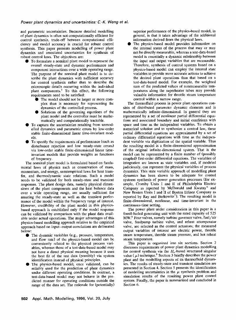
and parametric uncertainties. Because detailed modelling of plant dynamics is often not computationally efficient for control synthesis, trade-off between computational efficiency and model accuracy is crucial for robust control synthesis. This paper presents modelling of power plant dynamics and associated uncertainties for synthesis of robust control laws. The objectives are:

0 To formulate a nominal plant model to represent the overall steady-state and dynamic performance and component interactions over a wide operating range. The purpose of the nominal plant model is to describe the plant dynamics with sufficient accuracy for control synthesis rather than to describe the microscopic details occurring within the individual plant components.5 To this effect, the following requirements need to be satisfied:

0 The model should not be larger or more complex than is necessary for representing the dynamics of the controlled process.

0 Solutions of the governing equations of the plant model and the controller must be mathematically and computationally tractable.

0 To capture the uncertainties resulting from unmodelled dynamics and parametric errors by low-order stable finite-dimensional linear time-invariant models.

0 To specify the requirements of performance (such as disturbance rejection and low steady-state errors) via low-order stable finite-dimensional linear time- invariant models that provide weights as functions of frequency.

The nominal plant model is formulated based on fundamental laws of physics such as conservation of mass, momentum, and energy, semiempirical laws for heat transfer, and thermodynamic state relations. Such a model needs to be validated for both steady-state and transient responses. The plant design data, namely physical dimensions of the plant components and the heat balance data over a wide operating range, are usually sufficient for assuring the steady-state as well as the transient performance of the model within the frequency range of interest. However, credibility of the plant model in this physics- based approach is established only if the model response can be validated by comparison with the plant data avail- able under actual operations. The major advantages of this physics-based modelling approach relative to the empirical approach based on input-output correlations are delineated below:

0 The dynamic variables (e.g., pressure, temperature, and flow rate) of the physics-based model can be conveniently related to the physical process variables, whereas those of a test-data-based model may not have a direct physical meaning because it uses the best fit of the test data (possibly) via system identification instead of physical principles.

0 The physics-based model, once validated, can be reliably used for the prediction of plant dynamics under different operating conditions. In contrast, a test-data-based model may not behave in the predicted manner for operating conditions outside the range of the data set. The rationale for (potentially)

502 Appt. Math. Modelling, 1996, Vol. 20, July

superior performance of the physics-based model, in general, is that it takes advantage of the additional information derived from the physical laws.

0 The physics-based model provides information on the internal states of the process that may or may not be directly measurable, whereas a test-data-based model is essentially a dynamic relationship between the input and output variables that are measurable. Therefore, synthesis of control systems based on a physics-based model can employ the internal state variables to provide more accurate actions to achieve the desired plant operations than that based on a test-data-based model. For example, the weighted sum of the predicted values of nonmeasurable temperatures along the superheater tubes may provide valuable information for throttle steam temperature control within a narrow range.

The thermofluid process in power plant operations consists of distributed parameter dynamic elements and is mathematically infinite-dimensional. In general they are represented by a set of nonlinear partial differential equations and associated boundary and initial conditions with space and time as the independent variables. To obtain a numerical solution and to synthesize a control law, these partial differential equations are approximated by a set of ordinary differential equations with time as the independent variable via digitization of the spatial variable. Thus the resulting model is a finite-dimensional approximation of the original infinite-dimensional system. That is the model can be represented by a finite number of (possibly coupled) first-order differential equations. The variables of integration are known as state variables and, if modeled judiciously, can represent the physical variables of process dynamics. This state variable approach of modelling plant dynamics has been shown to be adequate for control systems synthesis of power generation processes (for example, Cromby Units I and II of Philadelphia Electric Company as reported by McDonald and Kwatny6 and New Boston Units I and II of Boston Edison Company as reported by Ray and Berkowitz’). The resulting model is finite-dimensional, nonlinear, and time-invariant in the continuous-time setting.

The power plant under consideration in this paper is a fossil-fueled generating unit with the rated capacity of 525 MW.8 Four valves, namely turbine governor valve, fuel/air valve, feedpump turbine valve, and reheat attemperator valve, are selected as the control actuators; the measured output variables of interest are electric power, throttle steam temperature, throttle steam pressure, and hot reheat steam temperature.

This paper is organized into six sections. Section 2 discusses requirements of power plant dynamics modelling for control synthesis via the &-based structured singular value (p) technique.’ Section 3 briefly describes the power plant and the modelling aspects of its thermofluid dynamics. The results of steady-state and transient simulation are presented in Section 4. Section 5 presents the identification of modelling uncertainties in the p synthesis problem and simulation results of the resulting power plant control system. Finally, the paper is summarized and concluded in Section 6.


2. Modelling requirements for p control synthesis

The problem of robust control synthesis via &-based structured singular value (p) is generally formulated in terms of the models of the nominal plant, the associated uncertainties in plant modelling, external disturbances, and the performance specifications4 Figure I shows the basic structure of a feedback control loop. A general configuration of robust control techniques, such as H, and CL, is presented in Figure 2 where G represents the nominal plant, K is the controller, A approximates the uncertainties, w is the perturbation input, z is the perturbation output, d is the exogenous input signal, e is the performance variables, u is the control input, and y is the measured plant output. Figure 3 shows how the plant perturbations, A(s), interact with the finite-dimensional, linear, time-invariant control system, M(s), which includes the nominal plant, G(s), and the controller, K(S), within a closed loop. The input to the closed loop control system, M(s), consists of all exogenous signals w that include the reference command(s) to be tracked, actuator and plant disturbances, and sensor noise. The output z of the control system M(s) consists of all plant variables needed for specifying the stability and performance crite- ria. In the definition of the structured singular value E_L~[M(.s,)] of the transfer matrix, M(s), at a given sO, the underlying uncertainty A(s) belongs to a set of matrices, A(s), which is prescribed to have a block diagonal structure with the three characteristics type of each block, total number of blocks, and dimension of each block.

In general, there are two types of blocks: repeated scalar blocks and full blocks. Let two nonnegative integers, S and F, represent the number of repeated scalar blocks and the number of full blocks, respectively. Two sets of positive integers, r,, r2,. . . , rs and m,, m2,. . . , mF are used to represent the dimensions of these blocks such that the ith repeated scalar block is SiZ, , where Z, is the ri X ri identity matrix and ai E C, and the jth full block belongs to C”‘J~“‘J, where Cm’” is the set of m X n complex matrices.

For any ME C”‘“, is defined as”.

its structured singular value Pi

1

Ph(~) E inf{(T(A): AE_~, det(Z-MA) =0} -

0 VAE_d, det(Z-MA) #O

(1)

Figure 1. Structure of the basic feedback loop system.

W 2

d -e

II- Y

Figure 2. General representation of a perturbed control system.

If the uncertainties arecharacterized in the additive form, then the actual plant G(S) and the nominal plant G(S) are related as

G(s) =G(s) +A(s) (4

where A(s) is the additive uncertainty that represents the possible discrepancy between the actual plant G(s) and the nominal plant G(S). The uncertainties can also be charac- terized in other forms such as

C(s) =G(s)[Z+A(s)]

input multiplicative uncertainty (3)

G(S) = [z+A(s)]G(s)

output multiplicative uncertainty (4)

The specification of the uncertainties A(s) consists of two components, namely the weighting function Wde,(~) and the normalized perturbation matrix A,,,(s) with unity H, norm (i.e., II A,,,(s) II 33 = supW (T[ A(jw)] < 1). Therefore, A(s) can be expressed as

In equation (2) the uncertainty A(s) is used to describe the discrepancy between the actual plant, G(S), and the nominal plant model, G(S). All such possible discrepancies between I?(S) and G(s) must be covered_by A(s). As a result, the larger the discrepancy between G(s) and G(s), the larger A( s> is. However, as A(s) is made larger, the design becomes more conservative with possible degrada- tion in the system performance but a more accurate G(S)

A

M

Figure3. Interconnection of perturbation model and the closed loop control system.

Appl. Math. Modelling, 1996, Vol. 20, July 503

Power plant dynamics and uncertainties: C-K. Weng et al.

will make A(s) smaller and the design will be less conservative. However, since most robust control synthesis ap- proached are linear techniques, the nonlinear plant dynamics cannot be described over an operating region by a linearized model G(s). Moreover, a very accurate model can be too complex to be directly useful for control synthesis. A major assumption of the p synthesis proce- dure is that the pertu@ation A(s) must be allowable; that is, the actual plant, G(s), and the nominal plant model, G(s), have the same unstable poles. In other words, A(s) should neither introduce any unstable poles into the system “_or cause any unstable pole-zero cancellation in forming G(s). The perturbation A(s) cannot include any unstable pole(s). Consequently, it is required that every unstable poles of the linearized plant must be included in the nominal plant model G(s).

3. Description of the power plant

A schematic diagram of plant operations is given in Fig- ure 4. At the full load condition, the power output is 525 MW. The plant maintains the throttle steam condition of pressure at 2,415 psi and temperature at 950°F and the hot reheat steam temperature at 1,OOO”F. The design and thermodynamic characteristics of this plant are largely similar to those of a high temperature gas-cooled reactor nuclear plant”*” with the following major exceptions: the nuclear reactor is replaced by a fossil-fueled furnace; and the helium circulating turbine, located between the high pressure turbine exhaust header and the cold reheat header, is eliminated. Therefore, the high pressure turbines discharge directly into the cold reheat header. A brief description of plant operation is given below.

ATV

CP

FAV

FP

GN

HT

LP

PTV

SG

I I

Figure 4. Schematic diagram of the fossil power plant.

Figure 5. Model solution diagram.

A pair of turbine sets, each consisting of a high pressure, an intermediate pressure, and a low pressure turbine on the same shaft, drives the respective synchronous generators which are electrically coupled to the power system grid. A single furnace serves to generate both superheat and reheat steam. The steam generator set consists of six identical units, each of which contains a main steam generator and a reheater. The six main steam generators receive compressed feedwater from the feedwater header and discharge superheated steam into the main steam header which in turn drives a pair of high pressure turbines. Exhaust steam from the pair of high pressure turbines is discharged into the cold reheat header which feeds the six reheaters. The superheated steam from all reheaters is mixed in the hot reheat header which in turn feeds a pair of intermediate pressure turbines. Exhaust steam from each intermediate pressure turbine is fed into the respective low pressure turbine, feedpump turbine, and deaerator. A train of feedwater heaters is fed by the bled steam from each low pressure turbine which in turn discharges low-quality low-pressure steam into its respective condenser. The con- densed steam from each condenser is pumped into the respective deaerator via a train of low pressure heaters which are modelled as a single heater. Warm feedwater from each deaerator is further pressurized by the respective pair of feedpumps which is driven by its own turbine. The feedpump turbine discharges into the respective condenser. All four feedpumps discharge into the feedwater header which supply the six main steam generators and the associated reheat attemperators.

Figure 5 shows a solution diagram to organize the model equations. Each block in this diagram represents a physical component or a group of components. The lines interconnecting the blocks indicate directions of information flow or model causality. The diagram also determines how the individual component models mathematically in-

504 Appl. Math. Modelling, 1996, Vol. 20, July


Table 1. List of state variables

State variables Symbol Unit

Steam density at main steam generator discharge Specific steam enthalpy at main steam generator discharge Steam density at high pressure turbine throttle Steam density at reheater inlet Specific steam enthalpy at high pressure turbine exhaust Average specific steam enthalpy at reheater Average tube wall temperature in reheater at mean radius Steam density at hot reheat header Specific steam enthalpy at hot reheat header Saturated water temperature in the lumped heater shell Specific enthalpy of saturated water in deaerator storage Steam pressure at intermediate pressure turbine extraction Steam pressure at low pressure turbine lumped extraction Feedwater flowrate Feedwater pump-turbine shaft speed Specific enthalpy of feedwater at main steam generator inlet Economizer length in main steam generator Economizer-evaporator length in main steam generator Average tube wall temperature in economizer at mean radius Average tube wall temperature in evaporator at mean radius Average tube wall temperature in superheater at mean radius Average specific internal energy of steam in superheater Average gas temperature in the furnace Attemperator spray water flowrate Normalized governor valve area Normalized feed pump turbine control valve area Normalized fuel/air valve area

RSX HSX RHS RHX HHX HRH TRHM RHR HHR THTS HDA PIP PLP WFP NFP HSGI LSGl3 LSG15 TSGZM TSG4M TSGGM USG6 TGAS WATSD AGV APT AFAV

Ibm/ft3 BTU/lbm Ibm/ft3 Ibm/ft3 BTU/lbm BTU/lbm “F Ibm/ft3 BTU/lbm “F BTU/lbm psia psia Ibm/sec radlsec BTU/lbm ft ft “F “F “F BTU/lbm “F Ibm/sec

terface with each other and ensures consistent causality for the complete set of equations defining the physical process of the power plant. Following the plant configuration in Figure 5 the task of plant modelling is accomplished in two steps: modeling of individual components or groups of components; formulation of an overall plant model by appropriate interconnection of the individual component models. Step 1 includes determination of steady-state solutions and component eigenvalues at various operating

Table 2. Nomenclature of process parameters

Process UNIT Symbol Parameters

Normalized valve area

Efficiency Steam flow

rate Gas flow rate Enthalpy Power Constant Length Speed Intermediate

variable Pressure Heat Density Entropy Temperature Internal energy Water flow rate Torque

Ibm/sec

Ibm/sec BTU/lbm

MW

ft radlsec

psia BTU

Ibm/ft3 BTU/lbm

“F BTU/lbm Ibm/sec

A

E F

G H J K

N 0

P Q R S T U W X

points. Steady-state solutions of individual models are verified with design data, and the eigenvalues are exam- ined for frequency range. Step 2 incorporates the sequen-

Table 3. Nomenclature of plant components

Plant Component Symbol

Attemperator Attemperator valve Condensor Deaerator Fuel/air valve Fossil-fueled furnace Feedwater pump Feedwater header

including trim valve Governor valve Electrical generator High pressure turbine Hot reheat header Main steam header Low pressure feedwater

heater High pressure turbine

exhaust Intermediate pressure

turbine Low pressure turbine Feedwater pump

turbine pump turbine valve Reheater Reheat turbine Main steam generator Main steam generator

discharge

ATS ATV CD DA

FAV FF FP FH

GV GN HP HR HS HT

HX

IP

LP PT

PTV RH RT SG sx



tial interconnection of component models according to the model solution diagram shown in Figure 5.

4. Steady-state and transient response of the model

Table 1 lists the 27 state variables of the model that represent the plant dynamics. The nomenclature of variables and plant components are listed in Tables 2 and 3, respectively. The following major assumptions were made to formulate the plant dynamic model:

0 uniform one-dimensional fluid flow over any cross- section;

l spatial discretization of a distributed parameter process via lumped parameter approximation;

l negligible axial heat transfer in the gas/air, water/steam, and tube wall material;

0 negligible compressibility and flow inertia in the gas/air path; and

l negligible pressure drop due to velocity and gravita- tional head in the gas/air and steam paths.

The steady-state values of eight different load operating points are listed in Table 4. To examine the dynamic characteristics of the nonlinear model, a series of transients were simulated for a step decrease in each of the control input variables. Typical results at 100% load are presented in Figures 6-9. In each case one of the valve areas was decreased by 5%. Dynamic responses were observed for a period of 300 sec. The step decrease was applied at time equal to 20 set to ensure the plant was at an equilibrium condition before the disturbance was applied. Simulation results, shown in Figures 6-9, are discussed below.

The equations of the plant dynamic model are listed in Weng (1994),3 and are not presented in this paper because of space limitation.

(i) Step decrease in the governor valve: The transient response for a step change in the governor valve stem position from 100 to 95% load is shown in Figure 6. Initially, due to the decrease in the steam path area, the flow through the governor valve to the impulse stage of the high pressure turbine is reduced, which causes the drop of electrical power output. Reduced valve area also in-

Table4. Steady-state plant data at different load levels

Load 100% 90% 80% 70% 60% 50% 40% 35%

State variables RSX 3.52585 HSX 1426.26 RHS 3.31702 RHX 1.38711 HHX 1337.71 HRH 1440.81 TRHM 1050.61 RHR 0.585647 HHR 1520.40 THTS 298.655 HDA 326.988 PIP 154.400 PLP 74.3271 WFP 1003.35 NFP 500.429 HSGI 338.365 LSGIS 178.401 LSG15 262.510 TSGZM 592.113 TSG4M 713.840 TSGGM 865.739 USG6 1176.73 TGAS 860.731 WATSD 0.999545 AGV 0.891929 APT 0.474311 AFAV 0.918688

Input variables AGVR 1.00150 APTR 0.474311 AFAR 0.918688 AATR 0.198509

Output variables THS 949.986 THR 999.990 PHS 2414.98 JGN 525.001

3.49068 3.45796 3.42850 3.39795 3.37614 3.35568 3.32788 1426.24 1426.27 1426.19 1426.91 1426.56 1426.61 1429.93

3.31703 3.31689 3.31714 3.31359 3.31513 3.31472 3.29594 1.26469 1.13973 1.01235 0.881119 0.748960 0.613758 0.542008

1338.69 1339.55 1340.16 1341.03 1341.02 1340.99 1342.91 1441.95 1443.06 1444.02 1445.42 1445.99 1446.71 1449.37 1044.23 1037.44 1029.91 1022.68 1013.08 1002.71 1001.58

0.533921 0.481018 0.427036 0.371329 0.315345 0.258128 0.227636 1521.66 292.803 320.064 141.332 68.1937

916.255 485.429 331.103 177.079 264.456 585.338 708.182 864.602 1179.31 853.339

2.13787 0.653481 0.465756 0.838304

1522.97 286.299

312.387 127.811 61.8151

826.950 471.511 323.183 176.036 266.273 578.521 702.705 863.411 1181.67 845.363

2.93809 0.510879 0.468948

1524.20 279.005 303.793 113.843 55.1907

735.441 458.884 314.462 175.302 268.002 571.595 697.398 862.048 1183.73 836.657

3.41002 0.409769 0.485884 0.673222 0.756542

1526.01 270.687 293.994 99.3655 48.2883

641.225 447.797 304.687 174.844 269.476 564.500 692.294 861.034 1185.97 826.977

3.58422 0.330272 0.522070 0.588218

1527.03 261.137 282.714 84.5661 41.1909

545.507 438.514 293.620 174.834 271.065 557.047 687.343 859.169 1187.38 816.096

3.51019 0.264665 0.591478

1528.33 249.796 269.189 69.3634 33.8625 447.593 431.255 280.568 175.228 272.510 549.000 682.591 857.281 1188.75 803.469

3.25026 0.207271 0.738670 0.412807 0.501443

1531.56 243.030 260.978 61.4483 30.0374

396.648 428.390 272.736 175.320 272.653 544.551 680.284 858.211 1191.24 796.114

3.01702 0.180168 0.893792 0.367732

0.894700 0.802300 0.707800 0.600000 0.488600 0.403300 0.371600 0.465756 0.468948 0.485884 0.522070 0.591478 0.738670 0.893792 0.638304 0.756542 0.673222 0.588218 0.501443 0.412807 0.367732 0.422893 0.577840 0.665151 0.691329 0.667782 0.608248 0.559284

949.956 949.997 949.880 950.934 950.412 950.480 955.235

999.937 999.922 999.713 1000.56 999.8 999.692 1004.48

2414.91 2414.93 2414.79 2415.21 2414.8 2414.79 2414.89

472.493 419.993 367.459 315.141 262.527 210.016 184.438



Tlmc e4 nm (ICC,

Figure 9. Transient response for a step decrease in the attemperator valve (AATR).

Figure 6. Transient response for a step decrease in the gover- nor valve (AGVR).

duces higher throttle steam pressure upstream of the valve. The throttle steam temperature rises because of the reduced water/steam flow and continued heat input at the previous rate. The increased steam temperature and pressure result in better turbine efficiency which causes an increase in the electrical power output and a higher reheat steam temperature.

(ii> Step decrease in the feedpump turbine valve: The transient response for a 5% step decrease in the feedpump turbine valve area from the initial full load condition is shown in Figure 7. As the feedpump speed decreases, the throttle steam pressure drops due to lower feedpump pressure. As the feedwater flow rate is reduced and the heat input remains unchanged, both the throttle steam and hot reheat steam temperatures increase. The electrical power output eventually increases due to improved thermodynamic efficiency resulting from higher steam temperatures. However, initially there is a small dip in electrical power output due to a rapid decrease in the throttle steam pressure.

(iii) Step decrease in the furnace valve: Figure 8 shows the response for a 5% step decrease in the furnace valve area. With less heat input, each of pressure, temperature, and electrical power output settles to a lower value as the feedwater flow rate remains approximately constant.

(iv> Step decrease in the attemperator valve: The response for a 5% step decrease in the attemperator valve area is shown in Figure 9. With less attemperator flow, reheat steam temperature increases. Less attemperator flow also implies a small increase in the feedwater flow through the main steam generator. Therefore, the throttle steam temperature slightly decreases, and the throttle steam pressure enjoys a small (about 1 psi) increase. Since the pressure dynamics is faster than the temperature dynamics, the electrical output initially increases due to a higher reheat steam temperature but subsequently settles down to a smaller value due to the lower thermodynamic efficiency resulting from reduced throttle and hot reheat steam temperatures.

;:;i !ipi 0 100 2w 300 Cl 1w 200 300

TIN MC) Tlrn (xc)

Figure 7. Transient response for a step decrease in the Feed- pump turbine valve (APTR).

Figure 8. Transient response for a step decrease in the fuel/air valve (AFAR).



5. Synthesis and simulation of the control system

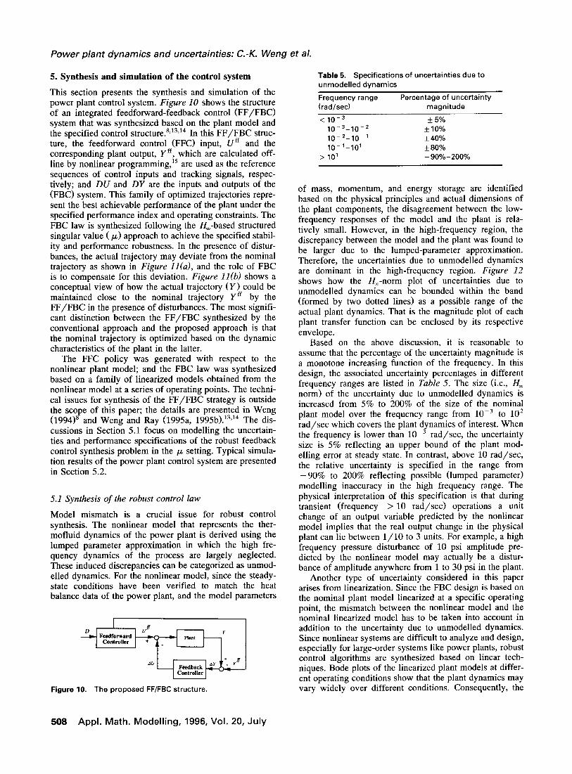
This section presents the synthesis and simulation of the power plant control system. Figure 10 shows the structure of an integrated feedforward-feedback control (FF/FBC) system that was synthesized based on the plant model and the specified control structure.8~‘3~‘4 In this FF/FBC structure, the feedforward control (FFC) input, Uff and the corresponding plant output, Y ff, which are calculated off- line by nonlinear programming,15 are used as the reference sequences of control inputs and tracking signals, respectively; and DU and DY are the inputs and outputs of the (FBC) system. This family of optimized trajectories represent the best achievable performance of the plant under the specified performance index and operating constraints. The FBC law is synthesized following the &-based structured singular value ( /.L) approach to achieve the specified stability and performance robustness. In the presence of disturbances, the actual trajectory may deviate from the nominal trajectory as shown in Figure 11(u), and the role of FBC is to compensate for this deviation. Figure 11(b) shows a conceptual view of how the actual trajectory (Y) could be maintained close to the nominal trajectory Yff by the FF/FBC in the presence of disturbances. The most signifi- cant distinction between the FF/FBC synthesized by the conventional approach and the proposed approach is that the nominal trajectory is optimized based on the dynamic characteristics of the plant in the latter.

The FFC policy was generated with respect to the nonlinear plant model; and the FBC law was synthesized based on a family of linearized models obtained from the nonlinear model at a series of operating points. The techni- cal issues for synthesis of the FF/FBC strategy is outside the scope of this paper; the details are presented in Weng (1994j8 and Weng and Ray (1995a, 1995b).13,14 The dis- cussions in Section 5.1 focus on modelling the uncertainties and performance specifications of the robust feedback control synthesis problem in the p setting. Typical simulation results of the power plant control system are presented in Section 5.2.

5.1 Synthesis of the robust control law

Model mismatch is a crucial issue for robust control synthesis. The nonlinear model that represents the thermofluid dynamics of the power plant is derived using the lumped parameter approximation in which the high frequency dynamics of the process are largely neglected. These induced discrepancies can be categorized as unmodelled dynamics. For the nonlinear model, since the steady- state conditions have been verified to match the heat balance data of the power plant, and the model parameters

1 I

Figure 10. The proposed FF/FBC structure.

Table 5. Specifications of uncertainties due to unmodelled dynamics

Frequency range Percentage of uncertainty (rad/sec) magnitude

< 10-3 f 5% 10-3-10-* *lo% lo-*-IOV’ f 40% lo-‘-lo’ +80%

> IO’ -9O%-200%

of mass, momentum, and energy storage are identified based on the physical principles and actual dimensions of the plant components, the disagreement between the low- frequency responses of the model and the plant is relatively small. However, in the high-frequency region, the discrepancy between the model and the plant was found to be larger due to the lumped-parameter approximation. Therefore, the uncertainties due to unmodelled dynamics are dominant in the high-frequency region. Figure 12 shows how the &-norm plot of uncertainties due to unmodelled dynamics can be bounded within the band (formed by two dotted lines) as a possible range of the actual plant dynamics. That is the magnitude plot of each plant transfer function can be enclosed by its respective envelope.

Based on the above discussion, it is reasonable to assume that the percentage of the uncertainty magnitude is a monotone increasing function of the frequency. In this design, the associated uncertainty percentages in different frequency ranges are listed in Table 5. The size (i.e., H, norm> of the uncertainty due to unmodelled dynamics is increased from 5% to 200% of the size of the nominal plant model over the frequency range from 10m3 to lo* rad/sec which covers the plant dynamics of interest. When the frequency is lower than 10e3 rad/sec, the uncertainty size is 5% reflecting an upper bound of the plant modelling error at steady state. In contrast, above 10 rad/sec, the relative uncertainty is specified in the range from -90% to 200% reflecting possible (lumped parameter) modelling inaccuracy in the high frequency range. The physical interpretation of this specification is that during transient (frequency > 10 rad/sec) operations a unit change of an output variable predicted by the nonlinear model implies that the real output change in the physical plant can lie between l/10 to 3 units. For example, a high frequency pressure disturbance of 10 psi amplitude predicted by the nonlinear model may actually be a disturbance of amplitude anywhere from 1 to 30 psi in the plant.

Another type of uncertainty considered in this paper arises from linearization. Since the FBC design is based on the nominal plant model linearized at a specific operating point, the mismatch between the nonlinear model and the nominal linearized model has to be taken into account in addition to the uncertainty due to unmodelled dynamics. Since nonlinear systems are difficult to analyze and design, especially for large-order systems like power plants, robust control algorithms are synthesized based on linear techniques. Bode plots of the linearized plant models at different operating conditions show that the plant dynamics may vary widely over different conditions, Consequently, the



(a) Nominal trajectory (b) Nominal trajectory

Actual trajectory Actual trajectory

Time Time Figure Il. (a) Plant trajectory under FFC. (b) Plant trajectory under FFC/FBC.

uncertainties due to linearization cannot be neglected for robust control analysis and synthesis over a wide operating range. Figure 13 shows a typical envelope of the Bode magnitude plots of a family of transfer functions within which the linearized models are located.

5.2 Simulation results

The FFC policy and the FBC law were combined to formulate an integrated FF/FBC system.8V13,14*16 Under nominal conditions, i.e., no perturbation and uncertainties, the simulation results of the FF/FBC system for power decrease are shown in Figures 14 15 for the transient responses of the plant output and input variables, respectively. Figure 14 shows that, during the first 360 set for which the FFC was synthesized, there is no deviation between the actual trajectory and the optimal trajectory because no perturbation is injected into the nominal plant model. Therefore, during this period of 360 set, the FBC was inactive. However, after 360 set, the FFC inputs are held at the final values of the FFC sequence, which may not be identical to the steady-state control inputs corresponding to the terminal load. This is equivalent to injec- tion of a disturbance at the plant input starting from the instant of 360 sec. Now it becomes the responsibility of the FBC to maneuver and maintain the plant at the desired equilibrium point. The control system regulated deviations from the desired outputs and reached the steady state after

Envelope of the Plant Model plus Uncertainties

Frequency (radkec)

Figure 12. Y-norm Plot of uncertainty due to unmodeled dy- Figure 13. namics. THR.

N 15 min. The steady-state errors at outputs were observed to be urns < 2”F, ~~~~ < 3”F, cpHS < 6 psi, and cJoN < 1 MW. Similar results for power ramp up are shown in Figures 16 and 17.

In order to examine the performance of the control systems under perturbations, two types of parametric disturbances were injected. First, the time constant of each valve was made to be 1.5 times larger, that is 50% error in the dynamic response of each actuator. Physically this means that the movements of the valve actuators are 50% slower than those predicted by the model. Second, efficiency of the high pressure turbines, intermediate pressure turbines, and feedpumps were all reduced by 5%, that is 5% modelling error in these components. The variations in valve dynamics represent the uncertainties in modelling of the dynamic behavior. Since the impact of errors in time constants die out as the system approaches the steady state, this uncertainty primarily affects the high frequency components of the transient responses. On the other hand, a change in the turbine or pump efficiency influences the plant transients at all frequencies and has a strong bearing on both the steady-state and transient performance. The simulation results of the FFC system alone (i.e., with no feedback action) under plant perturbations are shown in Figure 18 in which solid lines represent the perturbed response and dotted lines represent the nominal FFC trajectories. The outputs are seen to deviate from the original respective optimized trajectories due to the injected perturbations. The variations in temperatures and pressure vio-

loot I lfl 10.' lo.’ IO” IO’ IO2 IO3

Frequency (radkec)

Bode plot of the transfer function from AGVR to

APP~. Math. Modelling, 1996, Vol. 20, July 509


Figure 16. Plant output responses of the FF/FBC system for power increase at lO%/min.

Figure 14. Plant output responses of the FF/FBC system for power decrease at lO%/min.

late the specified constraints under the FFC alone. This implies that the throttle steam and hot reheat steam temperatures could not be maintained within the desired ranges without a robust feedback controller.

A major feature of the FF/FBC structure is that, in addition to the coarse control provided by FFC, FBC

compensates for the deviations from the desired plant output trajectory by fine-tuning the control inputs. Pertur- bations, identical to those injected into the FFC system, were applied to the FF/FBC system to examine its robustness. Figures 19 and 20, respectively, show the input and output responses of the FF/FBC system for the first 360

I I I

Figure 17. Control input responses of the FWFBC system for power decrease at lO%/min.

Figure 15. Control input responses of the FF/FBC system for power decrease at lO%/min.



Figure 18. Plant output responses of the FFC system under perturbations.

set, under these perturbations where the perturbed responses and the nominal trajectories are represented by dotted lines and solid lines, respectively. It is seen in Figure 19 that the control inputs were automatically ad- justed by FBC to compensate for the deviations. As a result, the perturbations, the plant response closely fol-

1%

--------_

5 OS- ----.__

- Penurbcd system kSpo”Y ;

Figure 19. Control input responses of the FF/FBC system under perturbations.

Figure 20. Plant output responses of the FF/FBC system under perturbations.

lowed the nominal optimized trajectory as seen in Figure 20.

6. Summary and conclusions

This paper presents the interactions between robust control synthesis and modelling of plant dynamics and uncertainties in the context of wide-range operations of power generation systems. This concept is illustrated by an integrated FF/FBC policy that was synthesized based on models of the power plant dynamics, uncertainties, and performance specifications for load following operations of a 525 MW fossil-fueled generating unit. In the FF/FBC configuration, an optimal feedforward control policy was formulated based upon the nonlinear plant model, and the robust feedback control law was synthesized based on a family of linear models that were generated via linearization of the nonlinear model at a series of operating points. To this effect, a 27th order nonlinear time-invariant plant model was developed in the state-space setting based on fundamental laws of physics and lumped-parameter approximation. The requirements of modelling power plant dynamics for &-based structured singular value ( p) synthesis were taken into consideration to achieve a trade-off between modelling accuracy and computational economy. Conceivable sources of modelling uncertainties stemming from model derivation were identified. These uncertainties and the desired plant performance specifications were, in turn, represented by appropriate transfer matrices in the setting of /_L The results of simulation experiments show that the FF/FBC system satisfies the specified performance requirements of power ramp up and down in the range of 40-100% load under nominal conditions of load following operations.



It is concluded that, for robust control synthesis of large-scale systems, the plant dynamic model and identification of the modelling uncertainties and performance specifications should be simultaneously conducted because these tasks are strongly interrelated. For example, modelling uncertainties can often be reduced at the expense of the size and complexity of the plant model which makes the synthesis and implementation of the control system difficult. However, an overly simplified plant model may not be adequate to meet the performance specifications because the robust control law will have to be made sufficiently conservative to account for the modelling uncertainties.

Nomenclature

HW

EFD W

:

e

U

Y A(s) M(s)

G(s) K(s) S F

I,

w-norm Hardy space structured singular value computational fluid dynamics perturbation input perturbation output exogenous input signal performance variable control input measured plant output plant perturbations finite-dimensional, linear time-invariant control system nominal plant controller the number of repeated scalar blocks the number of full blocks the ri X ri identity matrix

lrnx n C the set of m X n complex matrices &(s) the weighting function Ye the nominal trajectory Y actual trajectory E steady-state error

References

1.

2.

3.

4.

5.

6.

7.

8.

9.

10.

11.

12.

13.

14.

15.

16.

Facchiano, A. Applications of computational fluid dynamics modeling in the design of industrial combustion systems, Combustion Modeling And Burner Replacement Strategies. ASME, Fuels And Combustion Technologies Division, Boston, 1990 Sloan, D. G. and Sturgess, G. J. Modeling of local extinction in turbulent flames. Proceedings of the International Gas Turbine and Aeroengine Congress and Exposition, Hague, Netherlands, 1994 TRAC-BDl-MODI: An Advanced Based Estimate Computer Pro- gram for Building Water Reactor Transient Analysis. Vol. 1, TRAC- BDl-MOD1 Users Manual, 1992 Packard, A. and Doyle, J. C. The complex structured singular value. Automatica 1993, 29, 71-109 Ray, A. Dynamic modelling of once-through steam generator for solar applications. Appt. Math. Modelling 1980, 417-423 McDonald, J. P and Kwanty, H. G. Design and analysis of boiler- turbine-generator controls using optimal linear regulator theory. IEEE Trans. Automat. Control 1973, AC-U(3), 202-209 Ray, A. and Berkowitz, D. A. Digital simulation of a commercial scale high temperature gas-cooled reactor (HTGR) steam power plant. ASME J. Dynamic Sys. Measure. Control 1979, December. 284-289 Weng, C. -K. Robust wide range control of electric power plants. Ph.D. Thesis, Pennsylvania State University, 1994 Zhou, K., Doyle, J., and Glover, K. Robust and Optimal Control. Prentice-Hall, New York, 1995 Doyle, J. C., Wall, J. E., and Stein, G. Performance and robustness analysis for structured uncertainty. Proceedings of the IEEE Confer- ence on Decision and Control, Orlando, FL, 1982 Ray, A. Mathematical modeling and digital simulation of a commercial scale high temperature gas-cooled reactor (HTGR) steam power plant. Ph. D. Thesis, Northeastern University, Boston, MA, 1976 Ray, A. and Bowman, H. F. Design of a practical controller for a commercial scale fossil power plant. IEEE Trans. Nucl. Sci., 1978, August, 1068-1077 Weng, C. -K. and Ray, A. Robust wide range control of electric power plants, IEEE Trans. Control Syst. Tech., in press Ray, A. and Weng, C. -K. Robust wide range control of steam-electric power plants. Electric Power Research Institute Report under Contract no. EPRI 8030-5, 1995 Gill, P. E., Murray, W., Saunders, M. A., and Wright, M. H. User’s Guide for NPSOL (Version 4.0): A Fortran Package for Nonlinear Programming. Stanford University, Stanford, CT, 1986 Weng, C. -K., Edwards, R. M., and Ray, A. Robust wide-range control of nuclear reactors by using the feedforward-feedback concept. Trans. Nucl. Sci. Eng., 117, 177-185


elsevier modelling of power plant dynamics and

Documents