modelling salt dynamics on the river murray floodplain in ... · 1.4 project aims 7 2 groundwater...
TRANSCRIPT

Modelling salt dynamics on the River Murray floodplain in South Australia:
Modelling approaches
EDITOR
Juliette Woods
CONTRIBUTORS
Flinders University: Juliette Woods, Tariq Laattoe
CSIRO: Peter Cook, Robert Bridgart, Dennis Gonzalez, Trevor Pickett, David Rassam, Chris Turnadge
DEWNR: Matt Gibbs, Chris Li, Carl Purczel, Virginia Riches, Linda Vears
Goyder Institute for Water Research
Technical Report Series No. 15/10
www.goyderinstitute.org

Goyder Institute for Water Research Technical Report Series ISSN: 1839-2725
The Goyder Institute for Water Research is a partnership between the South Australian Government through the Department of Environment, Water and Natural Resources, CSIRO, Flinders University, the University of Adelaide and the University of South Australia. The Institute will enhance the South Australian Government’s capacity to develop and deliver science-based policy solutions in water management. It brings together the best scientists and researchers across Australia to provide expert and independent scientific advice to inform good government water policy and identify future threats and opportunities to water security.
The following Associate organisations contributed to this report:
Enquires should be addressed to: Goyder Institute for Water Research
Level 1, Torrens Building 220 Victoria Square, Adelaide, SA, 5000 tel: 08-8303 8952 e-mail: [email protected]
Citation Woods, J (ed.) 2015, Modelling salt dynamics on the River Murray floodplain in South Australia: Modelling approaches, Goyder Institute for Water Research Technical Report Series No. 2015/10, Adelaide, South Australia Copyright © 2015 Flinders University. To the extent permitted by law, all rights are reserved and no part of this publication covered by copyright may be reproduced or copied in any form or by any means except with the written permission of Flinders University. Disclaimer The Participants advise that the information contained in this publication comprises general statements based on scientific research and does not warrant or represent the completeness of any information or material in this publication.

Goyder Technical report 2015/10 ii
Acknowledgements
This project was funded by the Goyder Institute for Water Research and supported by the SA Department of Environment,
Water and Natural Resources (DEWNR) and the National Centre for Groundwater Research and Training (NCGRT).
The project scope was developed by the project team with input from Judith Kirk (DEWNR), Neil Power (DEWNR/Goyder), Wei
Yan (DEWNR), Kate Holland (CSIRO), Glen Walker (CSIRO), and Paul Dalby (In Fusion Consulting).
The Project Management Team for the project consisted of: Juliette Woods and Tariq Laattoe of Flinders University, Kate
Holland and Peter Cook of CSIRO, and Wei Yan, Matt Gibbs, Linda Vears, and Graham Green of DEWNR.
The Policy Advisory Committee for this project was chaired by Judith Kirk with Linda Vears as Executive Officer, both from
DEWNR. Other members were Danni Oliver of the Goyder Institute, Okke Batelaan of Flinders University, and Tony Herbert,
Chris Wright, Dragana Zulfic, Tumi Bjornsson and Whendee Young of DEWNR.
Many people contributed data, reports and discussion. Our thanks to Sina Alaghmand (University of South Australia & Monash
University), Nathan Clisby (DEWNR), Ed Collingham (formerly of SA Water), Russell Crosbie (CSIRO), Rebecca Doble (CSIRO),
Peter Forward (SA Water), Matt Gibbs (DEWNR), Graham Green (DEWNR), Huade Guan (Flinders), Hugo Gutierrez-Jurado
(Flinders), Tony Herbert (DEWNR), Jarrod Kath (University of Canberra), Chris Li (DEWNR), Matt Miles (DEWNR), Leanne Morgan
(Flinders), Tim Munday (CSIRO), Bob Newman (CMC Consulting), Ian Overton (CSIRO), Dan Partington (Flinders University),
Barry Porter (formerly of SA Water), Leike van Roosmalen (DEWNR), David Thompson (DEWNR), Chris Turnadge (CSIRO), Linda
Vears (DEWNR), and Wei Yan (DEWNR).
The following people contributed to Workshop 2: Steve Barnett (DEWNR), Okke Batelaan (Flinders), Kittiya Bushaway (DEWNR),
Alison Charles (AWE), Matt Gibbs (DEWNR), Graham Green (DEWNR), Nikki Harrington (Flinders), Kate Holland (CSIRO), Chris Li
(DEWNR), Dan McCullough (DEWNR), Hugh Middlemis (HydroGeoLogic), Leanne Morgan (Flinders), Dan Partington (Flinders),
Carl Purczel (DEWNR), Lieke van Roosmalen (DEWNR), and Linda Vears (DEWNR).
The principal external reviewers were Glen Walker (NCGRT) and Anthony Knapton (CloudGMS). Danni Oliver provided
comments on the May 2015 draft.
Le Dang (AWE) assisted with some figures and report compilation.
Amanda Nixon of Flinders University and Jason Tan of eResearch SA arranged collaborative data storage.
Nikki Harrington of Flinders University provided sound advice.

Goyder Technical report 2015/10 iii
Contents
1 Introduction 1
1.1 Study area and scientific context 1 1.2 Policy context 3 1.3 Current SA government models of River Murray hydrology and hydrogeology 3 1.3.1 Groundwater models 3
1.3.2 Surface water models 4
1.3.3 Need for improved capabilities 5
1.4 Project aims 7
2 Groundwater modelling approaches 9
2.1 Exemplar floodplain models 9 2.1.1 The Chowilla floodplain model 9
2.1.2 The Murtho climate sequence model 12
2.1.3 The Lindsay-Walpolla (EM4) floodplain model 13
2.1.4 The Shahse River Valley model 16
2.1.5 The Clarks Floodplain MODFLOW model 17
2.1.6 The Clarks Floodplain HydroGeoSphere model 20
2.1.7 Cross sectional Chowilla floodplain inundation model 21
2.2 Groundwater model platforms 24 2.2.1 Software 24
2.2.2 Single model, multi model and integrated model approaches 25
2.3 Modeling processes 26 2.3.1 Regional inflows 26
2.3.2 Evaporation and transpiration 26
2.3.3 River level change 28
2.3.4 Inundation Recharge (includes flood and artificial watering) 29
2.3.5 Evaporation from surface waters (includes interaction with wetlands) 32
2.3.6 Processes not modelled 33
2.4 Data requirements and availability for floodplain groundwater modelling 34 2.5 Discussion 46 2.5.1 Monitoring recommendations 46
2.5.2 Groundwater modelling priorities 47
3 Surface water modeling approaches 49
3.1 Introduction 49 3.2 Hydrodynamic Models 49 3.2.1 1D and Quasi 2D Hydrodynamic Approaches 49

Goyder Technical report 2015/10 iv
3.2.2 1D Hydrodynamic River Model and 2D Floodplain Reservoir Model 50
3.2.3 Full 2D Hydrodynamic Approaches 52
3.2.4 Hydrologic Models 53
3.3 Combining Hydrodynamic and Hydrologic Models 55 3.4 Discussion 57
4 Groundwater model trials 59
4.1 Model Conceptualisation 60 4.1.1 Hydrogeology 61
4.1.2 Surface Water 65
4.1.3 Base case conceptualisations 65
4.2 Base Model Construction, Validation and Initial Findings 66 4.2.1 Model code 66
4.2.2 Domain and Grid 66
4.2.3 Initial conditions and stress periods 66
4.2.4 Model Layers 67
4.2.5 Hydraulic Parameters 69
4.2.6 Boundary Conditions 71
4.2.7 Validation of Base Models 75
4.2.8 Findings from Base Models 79
4.3 Scenarios 80 4.3.1 River Scenarios 80
4.3.2 Evapotranspiration Scenarios 86
4.3.3 Inundation Scenarios 89
4.4 Scenario Results and Discussion 92 4.4.1 Scenario 1 - River Scenario 94
4.4.2 Scenario 2- Evapotranspiration Scenario 100
4.4.3 Scenario 3 - Inundation Scenario 106
4.5 Discussion 120
5 Surface water model development 122
5.1 Introduction 122 5.2 Theory 123 5.2.1 Introduction 123
5.2.2 Pressure Response 124
5.2.3 Transport Response 126
5.2.4 Mass Balance Correction 126
5.2.5 Regional Groundwater Flow 127

Goyder Technical report 2015/10 v
5.3 Implementation 127 5.3.1 Outline 127
5.3.2 Formulation 128
5.3.3 Example 1: Separate pressure and transport peaks 130
5.3.4 Example 2: Draining wetland model 139
5.3.5 Example 3: Coupled river model 150
5.3.6 Summary 156
5.4 Floodplain Groundwater Velocity and Travel Times 156 5.4.1 Outline 156
5.4.2 Formulation 157
5.4.3 Example 159
5.4.4 Summary 164
5.5 Discussion and conclusions 164
6 Conclusions and recommendations 166
6.1 Conclusions 166 6.2 Recommendations 167 6.2.1 Data and monitoring to support conceptual understanding and numerical models 167
6.2.2 MODFLOW modelling of saline floodplains 168
6.2.3 Further modelling 169
7 References 172

Goyder Technical report 2015/10 vi
List of figures
Figure 1-1 Extent and location of DEWNR’s groundwater models for the SA MDB ............................................................................................. 6 Figure 1-2 Location of the SA Murray Basin area ................................................................................................................................................................. 8 Figure 2-1 Conceptual model of the groundwater responses during and post flooding of the Chowilla floodplain ......................... 11 Figure 2-2 Information layers combined to define the model recharge zones (Source: Aquaterra) ........................................................... 11 Figure 2-3 Bore transects used to provide head measurements for calibration of the EM4 model (Source: Aquaterra, 2009) ...... 14 Figure 2-4 AEM slices identify flush zones and gaining reaches (Source: Aquaterra) ....................................................................................... 14 Figure 2-5 The spatially-distributed floodplain inundation recharge rates applied to the EM4 model (Source: Aquaterra) ........... 15 Figure 2-6 Conceptualisation of discharge and recharge in Doble et al. (2005) .................................................................................................. 18 Figure 2-7 Groundwater flux vs depth for various scenarios (Source: Doble et al. 2005) ................................................................................ 19 Figure 2-8 Maximum ET and recharge rates applied to Clark's Floodplain (Source: Alaghmand et al., 2014) ....................................... 20 Figure 2-9 Boundary conditions for the HydroGeoSphere model of Clark's Floodplain (Source: Alaghmand et al., 2014) .............. 21 Figure 2-10 Model grid and peizometric transects for the cross-sectional Chowilla model (Source: Jolly et al., 1998) ..................... 23 Figure 2-11 Comparison of the ET and ETS1 evapotranspiration functions (Source: Aquaterra) ................................................................. 27 Figure 2-12 Evapotranspiration zones in the EM4 model (Source: Aquaterra, 2009) ........................................................................................ 28 Figure 2-13 Example of FIM flood predictions ................................................................................................................................................................... 30 Figure 2-14 AEM slices and soil map used to produce the spatially-distributed recharge values for the EM4 model (Source:
Aquaterra) .......................................................................................................................................................................................................................................... 32 Figure 3-1 Quasi-2D approach to floodplain modelling, whereby the floodplain is simulated as branches of the main river
channel (Source: Huang et al., 2007). ..................................................................................................................................................................................... 50 Figure 3-2 Location of river reaches, cross-section and floodplain units (grey shaded regions) on the Purus River Basin, Brazil
(Source: Paiva et al., 2011). .......................................................................................................................................................................................................... 51 Figure 3-3 Wetting and drying process of floodplain elements of the raster model of Paz et al. (2011). Zf is floodplain elevation,
Za is water level, ha is surface water depth, hsub is water depth of soil reservoir, hres is the available volume of soil reservoir,
which has a maximum capacity equal to Hsmax. .................................................................................................................................................................. 51 Figure 3-4 Hysteretic relationship between river flow rate and floodplain inundation area, observed for the Koondrook
Perricoota Forest. Inundation area is higher for the same river flow rate on the falling limb of the flood (Source: Tuteja &
Shaikh, 2009). .................................................................................................................................................................................................................................... 53 Figure 3-5 Comparison of BIGMOD simulated salinity at Morgan with observation data for the period 1975 – 1999 (Source:
Telfer et al., 2012). ........................................................................................................................................................................................................................... 55 Figure 3-6 Relationship between modelled and observed inundation extent in a section of the Murrumbidgee River floodplain,
Yanga National Park, NSW (Source: Mackay et al., 2011). ............................................................................................................................................. 56 Figure 3-7 Comparison of the effect of grid cell size on simulation of inundation extent of the Murrumbidgee River in Yanga
National Park, NSW using a hydrodynamic model. Simulated floodplain inundation is much greater using a 20 m grid cell (blue
areas) than using a coarser 80 m grid (red and purple areas). (Purple areas are inundated in both models, and green areas are
uninundated.) (Source: Mackay et al., 2011). ....................................................................................................................................................................... 56 Figure 4-1 Model study area ...................................................................................................................................................................................................... 60 Figure 4-2 Simplified Floodplain Hydrogeology................................................................................................................................................................ 64 Figure 4-3 Goyder Floodplain Model Conceptualisation ((a): Broad Floodplain and (b): Broad Floodplain plus Highland) ............. 65 Figure 4-4 Surface Elevation Contours Case A and B ...................................................................................................................................................... 68 Figure 4-5 Surface Elevation Contours Case C ................................................................................................................................................................... 68 Figure 4-6 Thickness of Coonambidgal at Pike Floodplain based on existing bore data ................................................................................ 69 Figure 4-7 General Head Boundary Locations .................................................................................................................................................................... 71 Figure 4-8 Case A River position .............................................................................................................................................................................................. 74 Figure 4-9 Case B River position ............................................................................................................................................................................................... 74 Figure 4-10 Case C River position ............................................................................................................................................................................................ 75 Figure 4-11 Actual evapotranspiration out and groundwater level for Case A with lock ................................................................................ 77 Figure 4-12 Actual evapotranspiration out and groundwater level for Case A without lock ......................................................................... 78 Figure 4-13 Comparison of MODFLOW variants when simulating wetting of the Coonambidgal. ............................................................. 79 Figure 4-14 Measured River Level Data Upstream and Downstream of Lock 5 ................................................................................................... 81 Figure 4-15 River levels at different timesteps ................................................................................................................................................................... 85 Figure 4-16 Grid refinement around river ............................................................................................................................................................................ 86

Goyder Technical report 2015/10 vii
Figure 4-17 Potential evapotranspiration varies over time ........................................................................................................................................... 87 Figure 4-18 Spatial distribution of evapotranspiration .................................................................................................................................................. 88 Figure 4-19 ETS function used in Scenario 2G .................................................................................................................................................................... 89 Figure 4-20 Inundation at 16.0 m AHD for Case A with lock ...................................................................................................................................... 90 Figure 4-21 Inundation at 16.0 m AHD for Case A without lock................................................................................................................................. 91 Figure 4-22 Inundation at 16.0 m AHD for Case A with lock overlain on spatial distribution of inundation rate ................................ 91 Figure 4-23 Observation bores in models without a lock .............................................................................................................................................. 93 Figure 4-24 Observation bores in models with a lock ..................................................................................................................................................... 93 Figure 4-25 Hydrograph for Case A without lock ............................................................................................................................................................. 94 Figure 4-26 Net river condition for model A without a lock. ....................................................................................................................................... 94 Figure 4-27 Cumulative salt load for model A without lock. ........................................................................................................................................ 95 Figure 4-28 Downstream Lock 5 stage elevation for December 1996. .................................................................................................................... 96 Figure 4-29 Water balance for Scenario 1 model B without lock December 1996. ............................................................................................ 96 Figure 4-30 Cumulative salt load to river for model A with lock. Solute transport results are labelled with ST prefix. See
appendix for other modelled results. ..................................................................................................................................................................................... 97 Figure 4-31 Net river condition for model C with lock displaying large rapid gaining fluxes. See appendix for other modelled
results. .................................................................................................................................................................................................................................................. 98 Figure 4-32 Cumulative salt load to River with reservoir cell model ......................................................................................................................... 98 Figure 4-33 Net river condition for model C with a lock and reservoir cells ......................................................................................................... 99 Figure 4-34 Water Balance at 1996 for Case A with a lock ......................................................................................................................................... 101 Figure 4-35 Water Balance at 1996 for Case C without a lock ................................................................................................................................... 101 Figure 4-36 Comparison between linear ET curve and ETS curve with theoretic water table ...................................................................... 102 Figure 4-37 River Condition at 1996 for Case A with a lock ....................................................................................................................................... 103 Figure 4-38 River Condition at 1996 for Case C without a lock ................................................................................................................................ 103 Figure 4-39 Cumulative Salt Load for Case A with a lock, based on flow model .............................................................................................. 104 Figure 4-40 Cumulative Salt Load for Case A with a lock, based on solute model ........................................................................................... 104 Figure 4-41 Cumulative Salt Load for Case C without a lock, based on flow model ........................................................................................ 105 Figure 4-42 Cumulative Salt Load for Case C without a lock, based on solute model .................................................................................... 105 Figure 4-43 Hydrographs for Case A with a Lock ............................................................................................................................................................ 106 Figure 4-44 Hydrographs for Case C without a Lock ..................................................................................................................................................... 106 Figure 4-45 Water balance for Case A with lock under wet conditions. ................................................................................................................ 107 Figure 4-46 Water balance for Case A with lock under dry conditions ................................................................................................................. 107 Figure 4-47 Water balance for Case C without lock under wet conditions .......................................................................................................... 108 Figure 4-48 Water balance for Case C without lock under dry conditions ........................................................................................................... 108 Figure 4-49 River Condition for Case A with Lock .......................................................................................................................................................... 109 Figure 4-50 River Condition for Case C without Lock ................................................................................................................................................... 109 Figure 4-51 Cumulative Salt Load for Case A with a lock, based on flow model .............................................................................................. 110 Figure 4-52 Cumulative Salt Load for Case C without a lock, based on flow model ........................................................................................ 110 Figure 4-53 Cumulative Salt Load for Case A with a lock, based on solute model ........................................................................................... 111 Figure 4-54 Cumulative Salt Load for Case C without a lock, based on solute model .................................................................................... 111 Figure 4-55 Hydrographs for Case A with a Lock – near river, downstream of Lock ....................................................................................... 112 Figure 4-56 Hydrographs for Case C without a Lock – approximately 1 km from the river ......................................................................... 112 Figure 4-57 Watertable for Case A with a Lock at December 1996, Scenario 3A. ............................................................................................. 113 Figure 4-58 Evapotranspiration for Case A with a Lock at December 1996, Scenario 3A .............................................................................. 113 Figure 4-59 River boundary flux for Case A with a Lock at December 1996, Scenario 3A............................................................................. 115 Figure 4-60 Watertable for Case C with a Lock at December 1996, Scenario 3A .............................................................................................. 115 Figure 4-61 Evapotranspiration for Case C with a Lock at December 1996, Scenario 3A .............................................................................. 116 Figure 4-62 River boundary flux for Case C with a Lock at December 1996, Scenario 3A ............................................................................. 116 Figure 4-63 Watertable for Case A with a Lock at December 2006, Scenario 3A .............................................................................................. 117 Figure 4-64 Evapotranspiration for Case A with a Lock at December 2006, Scenario 3A .............................................................................. 117 Figure 4-65 River boundary flux for Case A with a Lock at December 2006, Scenario 3A............................................................................. 118 Figure 4-66 Watertable for Case C with a Lock at December 2006, Scenario 3A .............................................................................................. 118 Figure 4-67 Evapotranspiration for Case C with a Lock at December 2006, Scenario 3A .............................................................................. 119 Figure 4-68 River boundary flux for Case C with a Lock at December 2006, Scenario 3A ............................................................................. 119

Goyder Technical report 2015/10 viii
Figure 5-1 Conceptual model of the River Murray floodplain (Source: Holland et al., 2005). The red arrow indicates the flow and
transport pathway which is the focus of this chapter. ................................................................................................................................................... 123 Figure 5-3 Change in flow of water to the river following a short recharge pulse of 1 m
3 at a distance of 100 m from the river
(D= 10 m2/day). Both instantaneous (Equation 5-1; blue line) and cumulative (Equation 5-2; red line) fluxes are shown. ............ 125
Figure 5-4 Conceptual model of river and connected wetland. Surface water flow from the river to the wetland occurs when the
river stage exceeds the sill level and the wetland water level. Return flow from the wetland to the river occurs when the wetland
level exceeds both the sill level and the river level. Evaporation and infiltration remove water from the wetland and concentrate
salt. The distance from the river bank to the centre of the wetland (x) and the area of the wetland (A) are key model
parameters. ...................................................................................................................................................................................................................................... 128 Figure 5-5 Conceptual model used to investigate separate pressure and transport responses simulated using the modified
version of Source ........................................................................................................................................................................................................................... 130 Figure 5-6 (a) Water mass fluxes, (b) solute mass fluxes and (c) solute concentrations of water exiting the wetland (blue) and
groundwater (red). Note that the time scale is expanded for (a). ............................................................................................................................ 132 Figure 5-7 Sensitivity of (a) water mass flux, (b) solute mass flux, and (c) solute concentration of groundwater discharge to
changes in aquifer hydraulic conductivity. Note that the time scale is expanded for (a). ............................................................................. 133 Figure 5-8 Sensitivity of (a) water mass flux, (b) solute mass flux, and (c) solute concentration of groundwater discharge to
changes in aquifer thickness. Note that the time scale is expanded for (a). ........................................................................................................ 134 Figure 5-9 Sensitivity of (a) water mass flux, (b) solute mass flux, and (c) solute concentration of discharge to changes in aquifer
porosity. Note that the time scale is expanded for (a). ................................................................................................................................................. 135 Figure 5-10 Sensitivity of (a) water mass flux, (b) solute mass flux, and (c) solute concentration of groundwater discharge to
changes in aquifer specific yield. Note that the time scale is expanded for (a). ................................................................................................ 136 Figure 5-11 Sensitivity of (a) water mass flux, (b) solute mass flux, and (c) solute concentration of groundwater discharge to
changes in groundwater hydraulic gradient. Note that the time scale is expanded for (a). ......................................................................... 137 Figure 5-12 Sensitivity of (a) water mass flux, (b) solute mass flux, and (c) solute concentration of groundwater discharge to
changes in aquifer solute dispersivity. Note that the time scale is expanded for (a). ...................................................................................... 138 Figure 5-13 Solute mass (blue) and solute concentration (red) discharged from groundwater for scenario featuring high
specified groundwater concentration. ................................................................................................................................................................................. 139 Figure 5-14 Conceptual model used to test the performance of the modified Source software code (a) when realistic parameter
values were specified and (b) when regional groundwater flow was represented. .......................................................................................... 140 Figure 5-15 (a) Water mass fluxes, (b) solute mass fluxes and (c) solute concentrations of water exiting the wetland (blue),
groundwater link (red) and groundwater link 2 (green). Note that the time scale is compressed for (c). .............................................. 142 Figure 5-16 Sensitivity of (a) water mass flux, (b) solute mass flux, and (c) solute concentration of groundwater discharge to
changes in aquifer hydraulic conductivity. Note that the time scale is compressed for (c). ......................................................................... 144 Figure 5-17 Sensitivity of (a) water mass flux, (b) solute mass flux, and (c) solute concentration of groundwater discharge to
changes in aquifer thickness. Note that the time scale is compressed for (c). ................................................................................................... 145 Figure 5-18 Sensitivity of (a) water mass flux, (b) solute mass flux, and (c) solute concentration of discharge to changes in
aquifer porosity. Note that the time scale is compressed for (c). ............................................................................................................................. 146 Figure 5-19 Sensitivity of (a) water mass flux, (b) solute mass flux, and (c) solute concentration of groundwater discharge to
changes in aquifer specific yield. Note that the time scale is compressed for (c). ............................................................................................ 147 Figure 5-20 Sensitivity of (a) water mass flux, (b) solute mass flux, and (c) solute concentration of groundwater discharge to
changes in groundwater hydraulic gradient. Note that the time scale is compressed for (c)...................................................................... 148 Figure 5-21 Sensitivity of (a) water mass flux, (b) solute mass flux, and (c) solute concentration of groundwater discharge to
changes in aquifer solute dispersivity. Note that the time scale is compressed for (c). ................................................................................. 149 Figure 5-22 Conceptual model used to represent river–wetland–groundwater interactions for testing of the modified version of
Source ................................................................................................................................................................................................................................................ 150 Figure 5-23 Fluxes of water (a) entering the model at the river inflow node, (b) diverted to the wetland storage node via the
wetlands hydraulic connector (WHC) node, and (c) flowing downstream from the WHC node. ............................................................... 153 Figure 5-24 (a) Water mass fluxes, (b) solute mass fluxes and (c) solute concentrations of water exiting the wetland (blue) and
the groundwater domain (red). Note that the time scale is compressed for (c). ............................................................................................... 154 Figure 5-25 Wetland salt mass storage ............................................................................................................................................................................... 155 Figure 5-26 Schematic representation of groundwater flow from a wetland to a river. The wetland leakage flux is qw, and the
flux to the river is vb. Both quantities have units of L2/T, and represent fluxes per metre length of river. .......................................... 158
Figure 5-27 River and wetland levels, flow rate between the river and the wetland and leakage rate beneath the wetland for a
sill height of 16 m. The leakage rates form the input flux for the groundwater flow module in each of the different models. ... 160

Goyder Technical report 2015/10 ix
Figure 5-28 Salt flux leaking beneath the wetland, and salt flux to the river under three different groundwater flowpath
conceptualisations. Note that y-axis scales are logarithmic. ...................................................................................................................................... 161 Figure 5-29 Salt flux leaking beneath the wetland , and salt flux to the river under three different groundwater flowpath
conceptualisations. This figure contains the same data as Figure 26, except that salt flux is shown using a linear scale. Because
of this, some of the smaller salt fluxes are not visible on this figure. ..................................................................................................................... 162 Figure 5-30 Water and salt flux beneath the wetland for a single filling and draining event ...................................................................... 162 Figure 5-31 Salt flux leaking beneath the wetland, and salt flux to the river under four different groundwater flowpath
conceptualisations. The travel time of leakage is shown for each of the models, for two particular leakage events. Salt flux to
the river is not shown for the first 25,000 days, due to model warm-up (i.e. equilibration of initial conditions). ............................... 163

Goyder Technical report 2015/10 x
List of tables
Table 2-1 Data requirements for a floodplain groundwater model .......................................................................................................................... 35 Table 4-1 Hydraulic parameters from previous studies .................................................................................................................................................. 63 Table 4-2 Goyder Floodplain Model – Base Model Conceptualisations .................................................................................................................. 65 Table 4-3 Hydraulic Parameters used in the Goyder Floodplain Model .................................................................................................................. 70 Table 4-4 Solute transport model parameters ................................................................................................................................................................... 71 Table 4-5 General Head Boundaries ....................................................................................................................................................................................... 72 Table 4-6 Model constraint results for models without locks ...................................................................................................................................... 76 Table 4-7 Model constraint results for models with locks ............................................................................................................................................. 76 Table 4-8 River Scenarios............................................................................................................................................................................................................. 82 Table 4-9 Reservoir Scenarios .................................................................................................................................................................................................... 83 Table 4-10 Temporal discretisation rules for river boundary scenarios ................................................................................................................... 84 Table 4-11 Evapotranspiration Scenario Outline ............................................................................................................................................................... 87 Table 4-12 Inundation Scenarios .............................................................................................................................................................................................. 89 Table 5-1 List of symbols used ................................................................................................................................................................................................ 129 Table 5-2 Model parameter values. ....................................................................................................................................................................................... 130 Table 5-3 Model parameter values ........................................................................................................................................................................................ 140 Table 5-4 Model parameter values. ....................................................................................................................................................................................... 152 Table 5-5 List of groundwater parameters for different models .............................................................................................................................. 159 Table 6-1 Preliminary recommendations for MODFLOW modelling of SA River Murray floodplains ...................................................... 168 Table 6-2 Recommendations for further work using the MODFLOW model of Chapter 4 ........................................................................... 169 Table 6-3 Recommendations for groundwater modelling using other models and model platforms .................................................... 170 Table 6-4 Recommendations for Source model .............................................................................................................................................................. 171

Goyder Technical report 2015/10
Executive summary
The River Murray is the principal river of the western Murray Basin in southeastern Australia. It is highly unusual as it is a major
river system that flows through an extensive landscape with highly saline groundwater. The river is naturally prone to salinity,
and this propensity has increased over the past century due to the construction of river locks and the introduction of large-
scale land clearance and irrigation. River flow volumes and river level variability have been reduced, while the watertable has
risen. The overall impact has been to degrade riverine ecosystems and increase river and floodplain salinity.
Management of the lower River Murray floodplain requires a detailed understanding of its hydrological and hydrogeological
processes, including those which mobilise or store salt. The Basin Plan increases State obligations to manage and report on
salinity and water quality targets for the River Murray. A major outcome of the Basin Plan is to deliver environmental flows to
help protect and restore River Murray wetlands and floodplains. To do so effectively, SA must understand the short-term
movement of water and salt within the floodplain landscape, under present conditions and under various management options
for delivering environmental water.
Much research has been undertaken to monitor, conceptualise and simulate the dynamics of floodplain salinity. However, there
is currently no consistent and comprehensive approach to modelling the interaction of surface water and groundwater in the
lower River Murray floodplains. To address this need, in 2014 the Goyder Institute for Water Research commissioned the study
Modelling salt dynamics on the River Murray floodplain in South Australia, a collaborative research project with contributions
from Flinders University, CSIRO Land and Water, and the Department of Environment, Water and Natural Resources (DEWNR).
The study area consists of the floodplains of the River Murray in South Australia, from the Border to Morgan, within the South
Australian part of the Murray Basin. Due to the breadth of the review required, feedback was sought from a wide range of
experts and stakeholders.
The companion report, Modelling salt dynamics on the River Murray floodplain in South Australia: Conceptual model, data review
and salinity risk approaches (Woods, 2015a), documents the resulting conceptual model, data review, and salinity risk
methodology discussion. This report documents the literature review and testing of modelling approaches. A third report
contains the Appendices (Woods, 2015b).
Review of current approaches to groundwater modelling
Physically-based numerical groundwater models of floodplains or floodplain processes in Australia have been developed
predominantly with the industry standard groundwater model MODFLOW and in some cases its solute transport counterpart
MT3DMS. Other models have also been utilized on occasion such as SUTRA. There are a growing number of hydrologic models
that are capable of simulating integrated surface and sub-surface flow, such as HydroGeoSphere and MIKE SHE, but these have
rarely been used to simulate saline floodplains.
The majority of DEWNR’s groundwater models of the SA River Murray were developed to meet the requirements of the Basin
Salinity Management Strategy, and therefore focus on the long-term impacts of land use change and salt interception schemes
on River Murray salinity. With the exception of the Chowilla model, they are not designed to simulate floodplain processes in
any detail.
A literature review identified seven existing groundwater models of saline floodplains which include potentially useful
modelling approaches. These are the Chowilla floodplain model (Yan et al., 2004; RPS Aquaterra, 2012), the Murtho SIS climate
sequence model (AWE, 2010), the Lindsay-Walpolla (EM4) model (Aquaterra, 2009), the Shashe River Valley model (Bauer et al.,
2006), the Clarks floodplain MODFLOW model (Doble et al., 2005), the Clarks floodplain HydroGeoSphere model (Alaghmand,
2014) and the cross sectional Chowilla floodplain inundation model (Jolly et al., 1998).
The models differ in how they simulate floodplain processes. Evaporation, transpiration and recharge may be modelled as a
combined function or as separate functions. A variety of different assumptions have been used to describe the
evapotranspiration rate as a function of depth to water. Zones for ET and recharge may be defined based on vegetation, soil
type, groundwater salinity, surface water model calculations of inundation area, and/or AEM data. Rates may be sourced from
soil properties or unsaturated zone simulations. River level change may be averaged over different time periods and simulated
using different MODFLOW boundary conditions. The models rarely simulate unsaturated zone processes directly or the impact
of density differences due to salinity gradients.

Goyder Technical report 2015/10 i
Groundwater models can be informed by a large number of different types of data. Monitoring programs to support
conceptual understanding and numerical groundwater models should depend on the aims of the project, budget and time.
Review of current approaches to surface water modelling
Surface water models include one and two-dimensional hydrodynamic models and hydrologic models. Many hydrodynamic
river models rely on the one-dimensional solution to the Saint-Venant equation, or one of its simpler approximations for flow
in the river. To model the floodplains, a quasi two-dimensional approach can be applied, in which the flooded areas are
modelled as separate 1D river branches. Other models use a 1D hydrodynamic model for the main river channel, and a
reservoir approach for the river floodplain. More complex models simulate river flows across floodplains using full two-
dimensional solution to the river hydrodynamic equations. In contrast, hydrologic models use hydrologic routing approach to
calculate flow, and rating curves are used to determine the relationship between river depth and flow rate. BIGMOD, IQQM,
REALM and Source are also examples of hydrologic models. These types of models typically have short run times, and so are
suitable for simulating large systems.
Hydrologic river models are frequently used to examine how changes in river management will impact on flows and salt loads.
However, these river models do not include many important groundwater processes, or they include them only in highly
simplified manner.
Trials of groundwater model approaches
MODFLOW with MT3DMS was selected as the groundwater modelling platform for reasons both conceptual and pragmatic.
MODFLOW is capable of simulating the key floodplain processes and is also currently DEWNR’s preferred groundwater
modelling platform. Given the short project timeframe and immediate need for groundwater modelling recommendations, it
was preferable to build on DEWNR’s existing capabilities rather than introduce a new groundwater modelling platform at this
stage.
A simplified MODFLOW/MT3DMS model of the SA River Murray floodplain was used to test different approaches to simulating
three key processes: river level change (i.e. river-groundwater interaction), evapotranspiration, and recharge from floodplain
inundation. Numerical experiments were performed to explore how process representation affects model outputs. Both
groundwater flow and solute transport were simulated. The model is designed to represent generic conditions for the SA River
Murray floodplain in the study area; where variations exist, the model uses parameters representative of Pike floodplain. Six
base case models were developed, to cover a range of hydrogeological conditions. The river may have losing, throughflow or
gaining conditions at low flow; there may be a river lock (i.e. change in weirpool height) in the centre of the floodplain, or there
may be no lock. MODFLOW version, temporal discretisation, parameter sensitivity and process representation were explored.
MODFLOW2000 had numerical difficulties in simulating groundwater flow in the clay Coonambidgal Formation.
MODFLOW2005 with the NWT solver and UPW package has a revised “rewetting” algorithm and was able to simulate
groundwater flow in the Coonambidgal.
The numerical experiments show that using yearly averages of river stage and/or ET does not capture seasonal and climactic
variations in potentiometric head. Monthly and sub-monthly stress periods do capture this behaviour. However, flux between
river and groundwater is very sensitive to stress period length, particularly cumulative flux, so sub-monthly stress periods are
preferable when flux is a key output.
Model results were sensitive to small changes in the representation of ET. ET parameters controlled whether a river was under
gaining or losing conditions in low flow periods. Changes in extinction depth and rate altered the amplitude of hydrographs,
while spatially-varying ET zones also altered the phase/timing of peaks and troughs in potentiometric head. A curved function
of ET with respect to depth to water had lower overall actual ET rates than a linear function with the same extinction depth and
maximum ET rate. Topographic detail also strongly influenced ET.
Freshening of groundwater by river water lowers groundwater salinity near the river, so a constant-salinity calculation may
overestimate the salt flux in a dynamic river system.
Trials of surface water model approaches

Goyder Technical report 2015/10 ii
This project has developed some simple routines for calculating salt loads to the river resulting from infiltration beneath
inundated floodplain areas. These routines have been developed for possible inclusion in river hydrologic models that are used
for water management purposes, and have been coded into a trial version of the Source river model. Although further testing
of these routines is required before they are used for river management, initial testing results are been very positive. The
inclusion of floodplain salt transport routines in a regional river flow model would allow the interaction between river flow, and
flow regulation and salt loads to be examined.
Discussion and recommendations
MODFLOW and Source are two of a large array of possible choices of models. The choice of model will be influenced by the
model aim, the key processes, and the accuracy with which the different models describe these processes. It will also be
influenced by the time required to construct and run the model, and the ability to carry out the required number of simulations
in the required time period. It will also be influenced by the familiarity of the modeller (and the modeller’s institution) with
different numerical codes.
Current approaches to modelling the lower River Murray and SA floodplains often involve the simulation of a single model
simulating a single hydrological domain, without comparison to models of other domains. For example, the SA Salinity Register
models of groundwater and the DEWNR/MDBA Source models of surface water are developed independently and their results
are not compared to each other. For a region with considerable interaction between groundwater and surface water, one may
also consider a multi-model approach, where separate models of different hydrological domains are co-developed to be
consistent with each other. Discrepancies would identify gaps in conceptual understanding and in data. Another option is to
use a fully-integrated model which simulates multiple domains simultaneously, which would require further data and the
development of expertise in these model platforms.
Recommendations include lists of:
Monitoring tasks which could inform modelling; a subset should be selected based on the model area and aims.
Preliminary recommendations for groundwater modelling of saline floodplains; these are being trialled in Pike
Floodplain model, which is currently under development by DEWNR.
Further scenarios that could be run using the generic floodplain groundwater model.
Further work on groundwater modelling that would require the use of other models and/or model platforms.
Recommendations for further work on Source simulations.

Goyder Technical report 2015/10 1
1 Introduction
Juliette Woods, Linda Vears & Matt Gibbs
The River Murray is the principal river of the western Murray Basin in southeastern Australia. It is highly unusual as
it is a major river system that flows through an extensive landscape with highly saline groundwater. The river is
naturally prone to salinity, and this propensity has increased over the past century due to the construction of river
locks and the introduction of large-scale land clearance and irrigation. River flow volumes and river level
variability have been reduced, while the watertable has risen. The overall impact has been to degrade riverine
ecosystems and increase river and floodplain salinity.
In South Australia (SA), the River Murray provides water for the city of Adelaide, numerous smaller towns,
industry, stock, irrigation, and floodplain ecosystems; hence the management of river salinity is vital for the
economy and the environment. In recent decades, State and Federal governments have invested in research,
engineering works and evidence-based policy to control the salinity. This has been extremely successful, and the
salinity of River Murray water in SA now meets legislative targets even under extreme conditions of drought and
flood. Given this success, the focus of salinity management has widened to include the management of floodplain
salinity, to improve the health of riparian ecosystems.
Management of the lower River Murray floodplain requires a detailed understanding of its hydrological and
hydrogeological processes, including those which mobilise or store salt. Much research has been undertaken to
monitor, conceptualise and simulate the dynamics of floodplain salinity. However, there is currently no consistent
and comprehensive approach to modelling the interaction of surface water and groundwater in the lower River
Murray floodplains.
To address this need, in 2014 the Goyder Institute for Water Research commissioned the study Modelling salt
dynamics on the River Murray floodplain in South Australia, a collaborative research project with contributions
from Flinders University, CSIRO Land and Water, and the Department of Environment, Water and Natural
Resources (DEWNR). The project consisted of two main tasks. Task 1 was a review of data and literature on salinity
risk assessments and floodplain modelling in the lower River Murray. Task 2 developed and tested methods of
simulating the salinity dynamics of the lower River Murray floodplain.
The companion report, Modelling salt dynamics on the River Murray floodplain in South Australia: Conceptual
model, data review and salinity risk approaches (Woods, 2015a), documents the resulting conceptual model, data
review, and salinity risk methodology discussion. This report documents the literature review and testing of
modelling approaches. A third report contains the Appendices (Woods, 2015b).
1.1 Study area and scientific context
The study area consists of the floodplains of the River Murray in South Australia, from the Border to Morgan. This
is within the South Australian part of the Murray Basin (Figure 1-2). Downstream of Morgan, there is little risk of
salinity because groundwater salinities are lower and there is little flow from groundwater to the river. The
Coorong, Lower Lakes and Murray Mouth (CLLMM) region is not included as its hydrology and hydrogeology are
significantly different. While the study area is within South Australia only, similar salinity dynamics exist as far
upstream as Nangiloc-Colignan in New South Wales and Victoria. More broadly, similar dynamics may be seen
for any freshwater river that interacts with saline groundwater. Hence the literature review includes studies of sites
in SA, interstate and overseas.
The SA River Murray lies within the westernmost part of the Murray Basin. The geology and hydrogeology is
summarised in Woods (2015a).

Goyder Technical report 2015/10 2
The dry climate is responsible for the high salinity of the regional groundwater, concentrating the small
proportion of salt in rainfall over tens of thousands of years (Herczeg et al., 2001). The regional groundwater is
typically 20,000 mg/l but can be above 100,000 mg/l (Telfer et al., 2012).
The lower River Murray is a linear oasis within this dry landscape. The river has carved a trench through the upper
sediments of the Murray Basin, dividing the topography into floodplain and “highland”. Within the trench, some
freshwater is provided by rain, but the majority is delivered by the River Murray via surface channels, episodic
flooding, and by freshening groundwater. The freshwater supports a diverse ecosystem, most strikingly the
riparian river red gums and black box eucalypts.
The movement of freshwater and salt within the floodplain is complex. The river brings freshwater from upstream.
Regional groundwater flows into the floodplain sediments, bringing salt. Evapotranspiration concentrates salts in
the soils and groundwater. Flow between the river and floodplain aquifer depends on the gradient between the
river level and the watertable, which changes over time and may reverse due to complicated interacting factors.
Anabranches and wetlands may store and release salt. The system is extremely dynamic, and responds strongly to
climatic conditions such as drought and flood. Woods (2015a) summarises what is known about floodplain
hydrological processes which mobilise or store salt.
The system is further complicated by anthropogenic change. The construction of river locks in the 1920s/1930s
altered the balance between river levels and groundwater levels, and changed some anabranches and wetlands
from ephemeral to permanent while drying out others. Large-scale irrigation withdraws substantial volumes from
the river. Land clearance and irrigation have increased recharge to groundwater, raising the watertable and
mobilising more regional salt to the floodplain. Overall, the impact has been to reduce the volumes of freshwater
flowing into the SA River Murray floodplains while increasing the volumes of saline groundwater flowing in. The
average and peak salinity of the lower River Murray increased and floodplain vegetation was damaged.
Numerous works to control salinity have been undertaken. Some aim to reduce the flow of regional saline
groundwater into the floodplain trench. These include controls on land clearance, the rehabilitation of irrigation
areas to minimise recharge to the watertable, and the construction of Salt Interception Schemes (SIS). Other
works alter the flow of freshwater within the floodplain, using regulators, weir pool manipulation, wetland
management, artificial/environmental watering and pumping from the floodplain aquifer.
Works to control regional long-term salinity have been informed by numerical models, which estimate the
impacts of management options. Regional-scale models of surface water include MSM-BIGMOD and Source.
Regional groundwater models include the SIMRAT rapid assessment tools and the more detailed Salinity Register
MODFLOW models. These models have been developed by or for DEWNR and the Murray Darling Basin
Authority, and are well-tested and comprehensively reviewed. They employ consistent assumptions across the
region.
Floodplain salinity control works have also been modelled, albeit on a case-by-case basis. However, in many
situations the salinity impacts of possible management actions are difficult to quantify due to limited data, the
complexity of the dynamics, and a lack of a standard approach. In these situations, the salinity impacts may
instead be evaluated using a risk assessment method.
There is a need to improve the simulation of salt dynamics in the SA River Murray floodplain. This will improve
our understanding and management of the floodplain and river. There are numerous prior studies to learn from
which can be trialled and evaluated. From this a consistent preliminary approach can be derived and later
improved upon incrementally.
Woods (2015a) concluded that there are several inter-linked challenges in modelling floodplain salt dynamics.
The dynamics are controlled by numerous processes and drivers, many of which interact, and some of which are
poorly understood. The processes and features may not be simulated well by standard codes. The dynamics
impact domains which are usually modelled separately: groundwater, unsaturated zone, surface water, and
atmosphere. Each domain requires specialist expertise and employs assumptions and conceptualisations that may
differ from those used in other domains. Each process will vary spatially, depending on conditions and on

Goyder Technical report 2015/10 3
heterogeneity. Each process will vary over time, some on a daily basis, others seasonally or over much longer
timeframes (Telfer et al., 2012). Finally, there may be insufficient data to characterise the floodplain of interest.
Nevertheless, scientific advances continue to be made and policy changes (Section 1.2) require the improvement
of modelling methods. Quantifying the salinity impacts on the river and floodplain is the primary challenge for
the next generation of SA River Murray groundwater models.
1.2 Policy context
Schedule B to the Murray-Darling Agreement establishes a requirement to identify, assess, report, monitor and
review management actions which cause a significant long term increase in the salinity of the River Murray at
Morgan. These actions must be entered onto the Murray-Darling Basin Salinity Registers.
The Basin Plan expands obligations to manage and report on short term salinity and water quality targets for the
River Murray. All River Operators and Environmental Water Managers must have regard for these targets when
making flow management decisions. Having regard for water quality targets must be done in the context of the
outcomes of the Basin Plan, to deliver environmental flows to help protect and restore River Murray wetlands and
floodplains while maintaining water quality for all water users.
To fulfil these requirements and to provide assistance to policy makers and environmental managers, South
Australia is seeking to improve understanding of the short-term movement of water and salt within the floodplain
landscape, under present flow conditions and under various alternate options for delivering environmental water.
1.3 Current SA government models of River Murray hydrology and
hydrogeology
1.3.1 Groundwater models
The majority of DEWNR’s groundwater models of the SA River Murray were developed to meet the requirements
of the Basin Salinity Management Strategy (BSMS), which is discussed in Section 1.2. The BSMS focuses on the
long-term impacts of land use change and salt interception schemes on River Murray salinity. Estimates of these
salinity impacts are recorded and reported in the BSMS Salinity Registers. Since the BSMS was agreed, South
Australia has developed a series of groundwater models to estimate salinity debits and credits for the Registers.
The models calculate the groundwater flux and salt loads to the floodplain edge and/or the river. The scale and
design of these models is suitable for estimating long-term, regional impacts.
The models are of two types: the rapid assessment tool SIMRAT and a suite of MODFLOW models.
SIMRAT was developed for the Murray-Darling Basin Commission (MDBC) and accredited in 2005 to assess the
salinity impacts of new irrigation (Fuller et al., 2005). It is programmed within a GIS framework, employing
analytical equations and geographically-distributed parameters. It calculates the change in flux and salt load from
the regional aquifers to the edge of the floodplain with the assumption that salt entering the floodplain enters
the river. This consistent and deliberately simple approach can be used in areas where there is a high uncertainty
in the hydrogeological factors which influence groundwater salt flux to the river. It is used in New South Wales
and Victoria as well as South Australia (Woods et al., 2015).
The MODFLOW models are collectively known as the SA Salinity Register models. They cover the following
reaches of the SA River Murray:
Chowilla floodplain, including areas in New South Wales, South Australia and Victoria (Yan et al., 2005)
SA Border to Lock 3, which includes the following sub-models:
o Pike-Murtho (Woods et al., 2014)

Goyder Technical report 2015/10 4
o Berri-Renmark (Yan et al., 2007)
o Loxton-Bookpurnong (Yan et al., 2011)
o Pyap to Kingston (Yan et al., 2008)
Woolpunda (Woods et al., 2013)
Waikerie to Morgan (Yan et al., 2012)
Morgan to Wellington (Yan et al., 2010).
These models have been used to assess impacts of native vegetation clearance, irrigation, improvements in
irrigation practice and infrastructure and the SIS. The Chowilla model has been used to assess the impact of a new
regulator on Chowilla Creek, so is designed somewhat differently. The Salinity Register models calculate the
groundwater flux and salt load to the SA River Murray. Each model is based on detailed hydrogeological
information. They are calibrated against observed potentiometric heads and other outputs are compared against
supplementary data sources, such as geophysics and in-river salinity surveys. Yearly timesteps are used. The grid
size is typically 125 m. River levels and evapotranspiration (ET) generally do not change over time; the exception is
the Chowilla model, which is described in greater detail later in Chapter 2. The models simulate groundwater flow
but not solute transport. DEWNR groundwater models of the SA River Murray are not connected in any way with
surface water models of the SA River Murray (the Chowilla model is again a partial exception).
The models and reports must be reviewed both internally and by external reviewers; if approved, they are said to
be “accredited” by the MDBA. In accordance with Schedule B of the Murray-Darling Basin Agreement, all models
which support salinity impact assessments are required to undergo a review at intervals of no more than 7 years.
The SA Salinity Register models have generally been revised, updated, recalibrated and re-accredited every five
years. As such, they embody the latest hydrogeological information. The SIMRAT model has not been revised
since its inception, although a recent review makes recommendations to improve and update it (Woods et al.,
2015).
DEWNR also develops other MODFLOW models for site investigations. An example is the cross-sectional model
of Clark’s Floodplain in Bookpurnong (Berens et al., 2009).
DEWNR is a government body which needs to make defensible decisions based on reliable software. At present,
DEWNR’s groundwater modelling expertise is concentrated in MODFLOW, but includes MT3DMS, Excel
spreadsheets, GIS, Python and R. MODFLOW remains the primary platform as it is the industry standard: robust,
well-tested, well-supported by its developers and third-party GUI developers, and with an open source code.
Other, more specialist codes generally simulate more complicated physics, solving nonlinear equations which are
prone to numerical instability. As such, DEWNR will continue to use MODFLOW as its first choice in groundwater
model platforms, but may employ other models where the physics requires it.
1.3.2 Surface water models
The Science, Monitoring and Knowledge Branch within DEWNR currently use a wide range of surface water
models of the SA River Murray and environs. Coupled 1D and 2D models are used to represent the floodplain
anabranches of Chowilla Creek, Pike River and Katarapko Creek (e.g. McCullough, 2013). Full 2D hydrodynamic
approaches are used to represent inundation in each weir pool, for example for assessing weir pool raising
scenarios (Macky & Bloss, 2012). Hydrologic models, such as the BIGMOD and Source models of the SA Murray
developed by the MDBA, are regularly used to assess the influence of barrage operations on water levels and
barrage flows based on a flow forecast at the SA border and a range of diversion and loss scenarios.
However, these models either do not simulate salinity impacts at all, or do so in a limited sense. It is possible to
model the transport of salt (advection and dispersion) in the hydrodynamic models, however this has not been
undertaken to date. This approach also requires fixed salt inputs to be applied, surface water – groundwater
interactions are not modelled explicitly currently. For the hydrologic models, salt transport is modelled in the
same way as BIGMOD, an approach which adopts fixed salt inputs and does not provide any predictive capability
to represent the change in river operations or flow delivery scenarios on in river salinity. More and more, river

Goyder Technical report 2015/10 5
operations are being undertaken along the river to enhance environmental outcomes, for example Chowilla
regulator operation and weir pool raisings at Lock 1 and Lock 2. The ability to simulate the potential effect of
these types of operations on river salinity within the models currently used is highly desirable to inform
management decisions.
1.3.3 Need for improved capabilities
The current generation of Salinity Register models are suitable for evaluating long-term, regional-scale impacts
on groundwater salt loads to the SA River Murray. They simulate regional hydrogeological processes, a low-flow
River Murray, and include a simple representation of the floodplain. MDBA reviewers have praised the models,
but note shortcomings of the overall conceptualisation. The omission of river and floodplain dynamics makes it
easier to analyse and interpret the model results, which is desirable given the models’ aim of Salinity Register
accounting, but may lead to systematic biases in calibrated parameters. The model developers and reviewers have
raised this repeatedly in recent years with the MDBA, but the consensus was to continue with the current
conceptualisation until sufficient resources were available to develop and trial a next generation model that
included river and floodplain dynamics.
Another reason for considering floodplain dynamics is that there have been changes in the management of lower
River Murray floodplains. A variety of techniques are being trialled to improve the health and robustness of
floodplain ecosystems. Weirpool manipulation, new regulators, artificial/environmental watering, and floodplain
pumping are being introduced. Examples include: the trials conducted at Bookpurnong in 2006, the Chowilla
regulator, Riverine Recovery Program works, and the seven-year SA Riverland Floodplains Integrated
Infrastructure Program (SARFIIP) which focuses on Pike and Katarapko floodplains. Groundwater models of the
floodplain would assist with the engineering design of such works and with the evaluation of their salinity risks.
Finally, the Murray Darling Basin Plan expands obligations to manage and report on short-term salinity and water
quality targets for the River Murray. The current Salinity Register models are not designed to simulate short-term
impacts.
For these reasons, South Australia is seeking to improve understanding of the short-term movement of water and
salt within the floodplain landscape, under present flow conditions and under various alternate management
options. It is likely that this will require the development of two types of models: rapid assessment tools and
detailed site-specific models. The rapid assessment tools could quickly provide rough estimates of salinity
impacts in areas where there is little data and/or little risk. The detailed, site-specific models could be used to aid
engineering design and to evaluate salinity impacts where risks are higher or where greater detail is needed.

Goyder Technical report 2015/10 6
Figure 1-1 Extent and location of DEWNR’s groundwater models for the SA MDB

Goyder Technical report 2015/10 7
1.4 Project aims
The Basin Plan increases State obligations to manage and report on salinity and water quality targets for the River
Murray. A major outcome of the Basin Plan is to deliver environmental flows to help protect and restore River
Murray wetlands and floodplains. To do so effectively, SA must understand the short-term movement of water
and salt within the floodplain landscape, under present conditions and under various management options for
delivering environmental water. Short-term salinity impacts, both positive and negative, should be calculated in a
way consistent with the requirements of the Basin Plan and Schedule B. Current tools do not simulate the
floodplain in the detail needed.
The project provides foundational knowledge, data and outcomes for existing and emerging environmental
programs, including the Murray Futures Riverine Recovery Program, the South Australian Riverland Floodplain
Integrated Infrastructure Program (SARFIIP) and future salinity management activities.
The companion report (Woods, 2015a) reviews the geology and hydrogeology of the Murray Basin, including
details of the SA floodplains of the study area. It presents a conceptual model based on a literature review of
floodplain salinity dynamics, identifying relevant physical processes, and the natural and anthropogenic drivers
which impact the processes. Woods (2015a) also reviews the available datasets and approaches to salinity risk
assessment.
The key outputs presented in this report are:
Literature review of approaches to simulating the dynamics of saline floodplains. Chapter 2 discusses
models focussed on groundwater dynamics, including a discussion of relevant datasets. Chapter 3
considers modelling approaches that are focussed on the surface water system.
Key floodplain processes are examined to determine how these can be simulated (Chapter 4 and 5). This
includes assessments of the impact on simulation accuracy of different assumptions/simplifications and
data limitations.
MODFLOW and Source pilot models are developed and tested to simulate lower River Murray and
floodplain dynamics in Chapters 4 and 5 respectively.
A works program is developed to prioritise improvements in the modelling required and inform targeted
data collation and scientific studies (Chapter 6).
The Appendices provide the Python and Fortran programs developed as part of this project. A further Appendix
provides results from the groundwater simulations. The modified Source program is not included in the
appendices as the Source program is a proprietary code owned by eWater.
Due to the breadth of the modelling required, feedback was sought from modelling experts and floodplain
management stakeholders. In February 2015, preliminary numerical models were presented to groundwater
modellers at a workshop and were subsequently discussed at a Policy Advisory Committee meeting. Details of
those consulted are provided in the Acknowledgements.
The key overall research outcome is how to represent floodplain processes to inform floodplain and river salinity
management, including estimates of the uncertainty introduced by model assumptions. The outputs will enable
the progressive development of models of the SA River Murray to simulate the impact of environmental actions
on groundwater flow and salinity, including exchanges with the River Murray and freshening of floodplain
aquifers. They will also inform models of other regions where surface water – groundwater interactions are
important.

Goyder Technical report 2015/10 8
Figure 1-2 Location of the SA Murray Basin area

Goyder Technical report 2015/10 9
2 Groundwater modelling approaches
Tariq Laattoe, Juliette Woods, Chris Li & Virginia Riches
To simulate the water and salt dynamics in the River Murray floodplain, we need to understand the geological
context, develop a conceptual model of the floodplain dynamics and review the available data. The companion
report, Woods (2015a), provided this overview and identified key processes as:
1. Regional groundwater inflows
2. Evapotranspiration
3. River level change
4. Floodplain inundation, natural
5. Floodplain inundation, artificial
6. Evaporation from surface water
This chapter identifies methods used in the literature to represent these processes in numerical groundwater
models. Section 2.1 discusses key floodplain groundwater models which include potentially useful modelling
approaches. Section 2.2 considers model software. Section 2.3 considers each key process in turn, and compares
different ways of simulating them. Section 2.4 considers which datasets are potentially useful at the different
stages of numerical model development. Finally, Section 2.5 makes recommendations for testing and adopting
simulation techniques. Some of the recommended techniques are tested in Chapter 4 while others relate to works
that would need to be addressed in parallel and subsequent projects, as discussed in the report
recommendations (Chapter 6).
2.1 Exemplar floodplain models
Exemplar models featured in this section have been selected on the basis of their simulated processes, those
identified as significant factors for salt mobilisation on the floodplains of the Lower Murray. We do not present all
model input parameters as our aim in this section is to highlight unique approaches used in the selected models.
Further details of the models are located in their referenced publications. The selected models are:
1. The Chowilla floodplain model (Yan et al., 2004; RPS Aquaterra, 2012)
2. The Murtho SIS climate sequence model (AWE, 2010)
3. The Lindsay-Walpolla (EM4) model (Aquaterra, 2009)
4. The Shashe River Valley model (Bauer et al., 2006)
5. The Clarks floodplain MODFLOW model (Doble et al., 2005)
6. The Clarks floodplain HydroGeoSphere model (Alaghmand, 2014)
7. Cross sectional Chowilla floodplain inundation model (Jolly et al., 1998)
2.1.1 The Chowilla floodplain model
The Chowilla model is one of the SA Salinity Register models (see Section 1.3) and was developed using
MODFLOW by Yan et al., (2004). The floodplain at Chowilla is well-recognized as a discharge area for regional
saline groundwater to the River Murray during floods. The development of the locks and weirs has increased the
adverse salinity impacts to the floodplain and the water quality of the River, including the anabranch complex.

Goyder Technical report 2015/10 10
Initially, the Chowilla model was similar to the other SA Salinity Register models in that it was used to simulate the
regional aquifer system under low flow River conditions and did not include the simulation of any flooding. The
model has been updated multiple times since its initial development and has been revised to assess the benefits
and impacts of various management schemes proposed to improve floodplain and River health. It is now
considered the benchmark floodplain model in SA. The data density available in the Chowilla region sets this
model apart from any of the other floodplain models considered in this section.
In 2005 to 2006 the model was used for the first time to simulate aquifer hydraulic response to flooding, both
natural floods and floods induced by the proposed Chowilla Regulator (Figure 2-1). The modelled results were
used to estimate groundwater salt load delivery to River and were also used by CSIRO to predict vegetation
health response (Overton, 2005). In 2007, the model was used to simulate aquifer response to flooding from a 30
year River Murray flow hydrograph (Howe et al., 2007). Fundamental model parameters were not altered from
those used in Yan et al. (2004) other than to simulate flooding.
The 2012 update (RPS Aquaterra, 2012) comprised several changes to model input parameters including:
1. Updated LiDAR topography which has resulted in changes to surface topography, flood inundation area,
stream levels and evapotranspiration.
2. Refinements of the groundwater salinity zones based on AEM data.
3. Clarification and documentation of the flood inundation recharge rates.
The model covers an area of approximately 55 km (east-west) by 45 km (north-south) and includes the western
part of Lake Victoria and the entire Chowilla floodplain. Minimum grid size is 76.5 m by 62.5 m on the floodplain
with maximum grid size of 305 m by 250 m near the model edges. It comprises 5 layers, 2 of which are combined
floodplain plus adjacent regional units and the remaining 3 layers form the regional aquifers beneath the
floodplain. Initial development in 2004 featured constant head cells for River and anabranch representation. The
2012 update has replaced these with river cells (a type of head dependent flux hydraulic boundary cell) from
MODFLOW’s River package. Variable streambed conductance for the anabranch creeks has also been
implemented to simulate the effects of increased wetted perimeter with increased water level. Evapotranspiration
rates implemented in the model range from 150 to 250 mm/yr (much less than 1 mm/d) with extinction depths
between 1.5 and 3 m. Potential ET for the area is given at 2,000mm/yr.
Simulating flood response in the Chowilla groundwater model requires estimates of (i) the extent of inundation
for a range of specified flows, (ii) River Murray and creek levels during and after floods, and (iii) recharge rates for
areas under inundation. The first two items were provided by a hydrodynamic model developed by Water
Technology (2009). Recharge rates for inundated areas were mapped to spatial zones provided by CSIRO after
Overton et al. (2005) which are based on soil profiles. The recharge zones ultimately input into the model are a
combination of the inundated area for a specific River flow and the inundation recharge zones (Figure 2-2).
Recharge rates were supplied by Overton et al., (2005) but were significantly lowered during model calibration.

Goyder Technical report 2015/10 11
Figure 2-1 Conceptual model of the groundwater responses during and post flooding of the Chowilla
floodplain
Figure 2-2 Information layers combined to define the model recharge zones (Source: Aquaterra)

Goyder Technical report 2015/10 12
The mean groundwater salinity in both the Chowilla 2007 and Chowilla 2012 models is similar (~25,000 mg/l),
however Chowilla 2007 has a single value applied to the entire model whereas Chowilla 2012 has a spatially
variable salinity based on AEM data (~25,000 mg/l on the western half of the Chowilla floodplain and ~35,000
mg/l on the eastern half). Other notable assumptions and simplifications of the model include:
1. A flat River Murray weir pool (no backwater curves).
2. A simplified River Murray flow hydrograph comprising monthly time steps and 20,000 ML/day flow
magnitude divisions with a river flow of 5,000 ML/day assumed between flood events.
3. Inundation areas and stream levels for flows of 80,000 and 100,000 ML/day are represented by pre-
locking conditions in the hydrodynamic model.
4. Anabranch bed conductance parameter values that increase as the water level in the anabranches
increases (representing increased wetted perimeter).
5. Evapotranspiration from deep-rooted floodplain vegetation in the flush zone represented by an area of
negative recharge.
Notwithstanding the conceptual uncertainties and knowledge gaps outlined above, the good match to measured
groundwater levels and salt loads achieved by the model would indicate that the level of model simplicity that
has been adopted is adequate. Moreover, the simplifying assumptions are all considered to be conservative as
they are inclined to result in over-prediction of salt load to River. However, the time steps dictated by the
simplified hydrograph used for river stage means that short term (sub monthly) events cannot be simulated.
2.1.2 The Murtho climate sequence model
As part of the design of the Murtho SIS, AWE (2010) considered the impact of floodplain processes on SIS
efficiency. A MODFLOW/MT3DMS numerical groundwater flow and solute transport model was constructed
which simulated variable river levels and floodplain inundation. The model illustrates processes of flood recharge
and recession, the impact of drought, and the mixing of fresh and saline groundwaters in the floodplain. ET was
simulated more simply, in that potential ET rates were held constant over time.
The level of the River Murray was simulated over the BSMS Benchmark Period, i.e. from 1975 to 2010, including
floods and droughts. Stress periods were hand-selected to match observed changes in river level, so that periods
of rapid change had shorter stress periods. Stress periods ranged from 11 to 750 days in length. The river level
was calculated for each stress period and each river kilometer based on observations from upstream of each lock
and digitized backwater curves. The river was simulated using reservoir cells. When active, reservoir cells are
identical to river cells except that they interpolate linearly between the level at the start of a stress period to the
end of the stress period, so timesteps within the stress period more accurately reflect changing river levels. The
base of the river was estimated from NanoTEM survey bathymetry data. Riverbed hydraulic conductivity was
determined during calibration.
Overbank flow was also represented using reservoir cells. Each floodplain cell was assigned an elevation, based on
LiDAR data, and a time series of river levels. The river levels assigned to a floodplain cell were those of the closest
river kilometer (a simplification of flood hydrodynamics). A floodplain cell became wet (flooded) whenever the
river level was higher than the elevation. The hydraulic conductivity of the floodplain reservoir cells was 10-3
m/day, representing the resistance of the Coonambidgal Formation.
Solute transport simulation assumed salinities based on the medians of observations. River Murray and flood
waters were fresh (368 mg/l), irrigation recharge 500 mg/l, and the initial regional groundwater salinity was
28,930 mg/l. The groundwater salinity changed over time due to irrigation recharge, flows from the River Murray,
overbank inundation, and ET.
The flow model was calibrated to hydrographs, the solute transport results were compared with geophysics data,
and estimates of salt movement from groundwater to the Murray were compared with independent estimates
from MDBA's BIGMOD model.

Goyder Technical report 2015/10 13
2.1.3 The Lindsay-Walpolla (EM4) floodplain model
[Note at the time of writing this section, no documentation on the EM4 model was made available by the Mallee
Catchment Authority. The details included in this section are based on the contents of conference presentations
by Hugh Middlemis at the GroundWater2010 conference.]
The Eastern Mallee 4 (EM4) model focuses on the Lindsay-Wallpolla floodplain downstream of the confluence
between the Murray and Darling Rivers at Wentworth past Lock 10 to the SA border. The role of the model was to
assist in making management decisions concerning environmental watering options under the MDBA’s program
‘The Living Murray”. The sub-regional scale model was originally developed by Aquaterra in 2008 (Aquaterra,
2009) and further refined in 2010 to obtain detailed information on floodplain salt mobilisation processes. It uses
MODFLOW-Surfact (a modified version of MODFLOW from Schlumberger) operating under Groundwater Vistas.
It is designed as a medium to high complexity model, suitable for floodplain management purposes in terms of
simulating the effects of environmental flows and related surface and groundwater interaction processes. The
model results are used to inform vegetation health assessments, as well as for salinity management.
The Lindsay-Wallpolla floodplain is a data-rich area, which includes LiDAR, AEM depth slices, CSIRO soil recharge
map [to be confirmed], vegetation health mapping, and 75 floodplain bores covering 15 transects perpendicular
to the river (Figure 2-3). These data sources, when combined with a hydrodynamic model, allowed for detailed
representation of floodplain processes.
The model has 100 x 50 m grid cells. Quarterly stress periods are used in which river stage and recharge are
adjusted. River stage is assigned an average level based on pool level, backwater and anabranch levels. Two key
processes that were required to be addressed to successfully model floodplain processes were floodplain
inundation recharge and evapotranspiration.
Floodplain inundation was modelled as follows. Floodplain inundation areas were provided by the hydrodynamic
model for a range of specified river flows. Floodplain inundation recharge rates were based on airborne electro-
magnetic (AEM) data (Figure 2-4). AEM slices at 3 separate horizons were used to assign four salinity index
classes. The product of the index values from each layer at any location is treated as a qualitative indicator of the
rate of recharge. Recharge classes of 1, 3 and 6 mm/day were assigned (Figure 2-5), based on Overton et al.
(2005) (pers com. H.Middlemis, 2014), similar to the Chowilla model, however the exact details are not currently
available. The new recharge rates greatly improved calibration to potentiometric head levels observed during the
more frequent periods of flooding during the mid-1990s.
The EM4 model also features spatially-distributed evapotranspiration rates and extinction depths. These were
developed from the AEM data and also from vegetation health mapping developed by SKM. A greater maximum
evapotranspiration rate was assigned to areas with denser and healthier vegetation, as obtained from analyzing
National Vegetation Change data (NVC) and total dissolved salts (TDS). 14 classes were defined with maximum
rates from 0 to 0.005 m/day implemented via the standard ET package in MODFLOW. This improved the model
capability to match the recession periods for up to 5 years post-flooding.
The AEM slices were also able to provide information on interaction between the groundwater and the River
Murray. The AEM datasets can identify losing and gaining conditions (similar to the NanoTEM) and determine the
location and shape of freshwater lenses around the river. This provides another opportunity to check if the model
replicated what was known about the system. The documents provided also identified that AEM was used to
refine the calculation of salt load to the river in other models in the EM group (the EM2 suite), however no details
of this process was included.

Goyder Technical report 2015/10 14
Figure 2-3 Bore transects used to provide head measurements for calibration of the EM4 model (Source:
Aquaterra, 2009)
Figure 2-4 AEM slices identify flush zones and gaining reaches (Source: Aquaterra)

Goyder Technical report 2015/10 15
Figure 2-5 The spatially-distributed floodplain inundation recharge rates applied to the EM4 model
(Source: Aquaterra)

Goyder Technical report 2015/10 16
2.1.4 The Shahse River Valley model
Bauer et al. (2006) present a model to simulate the formation of a large freshwater lens over centuries. It uses a
modified evapotranspiration package in MODFLOW and SEAWAT. Similarities between the hydrologic settings in
the lower River Murray and the Shashe River Valley make these modifications worthy of consideration for future
modeling projects in SA.
The Shahse River Valley is located in northern Botswana at the south eastern fringe of the Okavango Delta. The
regional climate is semi-arid with annual precipitation of 450 mm/yr. and potential evaporation of 1,500 mm/yr.
The river valley is flooded every year when the Okavango Delta floods. One of the primary features of this river
valley is a large freshwater lens that has been continuously exploited for domestic water supply. Reduced
flooding and increased withdrawals has resulted in a dramatic decline in the water levels and mobilisation of the
saline water (approximately 25 ppt.) from the deep saline aquifer surrounding the freshwater lens.
Similar to the floodplains of the lower River Murray, evaporation and transpiration in the Shashe River Valley are
considered to be key processes that dominate the water budget. Ensuring that the behavior of these processes is
accurately represented in a model is crucial.
Evaporation is mainly a function of depth to watertable, porous media properties and climatic conditions, while
transpiration is a function of many variables including climate vegetation type, vegetation cover, depth to
watertable and water quality. For a solute mass balance, the processes differ in the maximum concentrations
produced. Evaporation can increase dissolved concentrations to an upper limit given the solubility of the salts
while transpiration breaks down at significantly lower concentrations depending on the salt tolerance level of the
plants.
In the standard SEAWAT software, evaporation and transpiration are lumped into a single process in the ET
package described by 3 parameters only. Rmax, the maximum rate of evapotranspiration, S, the water level
elevation (given by the where the rate starts to decline which is usually the topographic surface, and D, the
extinction depth where the rate is zero (Equation 2-1).
(2-1)
The simplest relationship for R between S and D used in most models is linear, as displayed above; however,
recent investigations have shown that in most cases an exponential relationship better approximates the flux
behavior. Through some relatively simple code modifications to the source code of the ET package in MODFLOW
the following change can be implemented:
(2-2)
For the Shashe River valley simulation, this modification was not sufficient to reproduce system behavior and
further modifications were made to separate evaporation from concentration-dependent transpiration. The linear
relationship (Equation 2-1) was used for evaporation while the exponential (Equation 2-2) was used for
transpiration. Transpiration was further modified to have a variable Rmax value dependent on salt concentration
given by the following:
,max
,max
(0)( ) erfc
2 2
T
T
R c cTR c
(2-3))
Where RT,max (0) is the transpiration rate for freshwater (m/day), cT is a threshold concentration(kg/m3) and σ
(kg/m3) is a shape parameter describing the smoothness of the transition. Typical literature values for cT range
max
max
for
1 for
0 for
R R h S
S hR R S D h S
D
R h S D
max .exp for S h
R R h SD

Goyder Technical report 2015/10 17
between 2 and 8 kg/m3 (2,000 to 8,000 mg/l) and for σ between 0.5 and 4 kg/m
3 (500 to 4,000 mg/l). It should be
noted that the form of the reduction function is hypothetical and is selected for mathematical convenience;
notwithstanding, it is qualitatively similar to growth reduction functions commonly used in modeling literature.
Changes were also made to SEAWAT to reflect salt accumulation by evaporation and transpiration. For
evaporation, the uptake of salt into the unsaturated zone will be related to the salinity of the groundwater,
implying that salt will exit the modelled saturated zone. The significance of this effect is not made apparent in the
results. Transpiration from the watertable will remove water but leave some or all the salt behind. In SEAWAT the
respective source terms qE and qT are parameterised the following way.
(2-4))
Where cu,i are the concentrations of the water taken up by evaporation and transpiration (kg/m3) and Δz is the
thickness of the cell from which the flux is drawn. In this manner, if the uptake concentration is equal to the
aquifer concentration (c=cu,i) then no accumulation occurs which is a reasonable approximation for the case of
diffuse uptake of water linked to evaporation. If the uptake concentration is zero (cu=0), all salt is left behind in
the aquifer, which is a reasonable approximation for the case of diffuse uptake of water linked to transpiration.
These changes to the ET package can be made via modifications to the source code and were implemented
because geochemical data used in the calibration process could not be matched without salt accumulation
processes in specific areas. A similar condition exists on the floodplains of the Lower Murray and this approach is
therefore worthy of further investigation when using models that include explicit representation of salinity. While
physically more realistic than a lumped ET function, separation of evaporation and transpiration may only result in
significant effects when simulation times range from decades to centuries.
2.1.5 The Clarks Floodplain MODFLOW model
This floodplain model determines which areas of the floodplain vegetation are most at risk from long-term
salinity (Doble et al., 2005). It is also able to show rates of lateral recharge from the River to vegetation. It
provides a methodology for the spatial comparison of discharge.
Calibration was not included and precise input parameters from field data were not required. The methodology
utilizes existing and tested evapotranspiration theory, and incorporates it into a combined recharge-discharge
relationship that is implemented in MODFLOW. To develop a spatially-variable, depth-dependent function for
recharge-discharge, the model requires spatial information for vegetation, soil and groundwater salinity, as well
as flooding duration and frequency. The function is similar to the segmented evapotranspiration function of the
MODFLOW ETS1 package but also incorporates a recharge component. Its use leads to more accurate long-term
modeling of evapotranspiration and recharge processes. The referenced publication contains a significant amount
of theory that was used to develop the combined recharge discharge relationship. We will present only the
fundamentals and its implementation in MODFLOW in this report.
Clarks Floodplain at Bookpurnong was chosen as the study site, as increased irrigation in the adjacent highland
has led to significant salt accumulation and vegetation dieback on the floodplain. The climate is semi-arid, with
rainfall varying between 200 and 300 mm/yr, and potential evaporation of approximately 1,800 mm/yr. The
floodplain is approximately 5 km wide and features ephemeral creeks and a lagoon at the break of slope to the
highland.
Recharge on the floodplain is predominantly from flooding events where infiltration rates is presumed to
approach a constant value. Recharge is therefore dependent on the vertical conductivity of the soil and the length
of time that the surface is inundated. Equations are provided in Doble et al., (2005) to calculate the recharge from
a single flood event for certain soil parameters. Cumulative effects of multiple floods can therefore be made into
a single function. The final recharge function is therefore able to account for recharge from multiple flood events
without actually simulating the flood itself.
u,
u,
u,
( ) for
0 for
i i
i i
i i
R c cq c c
z
q c c

Goyder Technical report 2015/10 18
A method for calculating cumulative groundwater discharge through plant water uptake is also provided.
Discharge in this method is governed by depth to watertable, soil texture and moisture content, and the ratio
between groundwater chloride concentration and the threshold concentration for plant water uptake. The
functions are combined through simple addition. They are represented conceptually in Figure 2-6. The function
applies a net recharge or discharge to the model depending on whether the groundwater head is above the
ground (maximum evapotranspiration), between the surface and equilibrium depth (point (a): net
evapotranspiration), between the equilibrium depth and extinction depth (point (b): net recharge) or below the
extinction depth (max recharge). The equilibrium point is where recharge and discharge fluxes are equal to zero
in the long term. With this method it is possible to include varying recharge functions such as zero recharge when
the groundwater is at the surface.
Figure 2-6 Conceptualisation of discharge and recharge in Doble et al. (2005)

Goyder Technical report 2015/10 19
Figure 2-7 Groundwater flux vs depth for various scenarios (Source: Doble et al. 2005)
Figure 2-7 gives groundwater flux vs depth relationships for various floodplain vegetation soil and groundwater
scenarios RGZ4 is Red Gums on clayey soil with low salinity groundwater. BBZ3 is Black Box on sandy clay with
moderate salinity groundwater. L Z2 is Lignum on heavy clay with high salinity groundwater. GLZ1 is grassland on
heavy clay with extremely shallow highly saline groundwater. RG FO Z3 is Red Gums with heavy clay flood out
and moderate salinity groundwater.
The maximum ET and recharge rates are given in Figure 2-8.
There may be opportunities for this methodology in floodplain management scenarios featuring artificial
inundation. The ability to simulate an actual flood or flooded area is a significant complication for model
development. Spatial and temporal discretisation of the modelled domain requires careful consideration when
attempting to capture the salt mobilisation processes from inundation scenarios. However, if the purpose of the
model is to determine changes in flux to the River from regulator operations and environmental watering
strategies over longer periods of time, then the combined recharge discharge approach provides a convenient
method to incorporate inundation events into a net long-term spatially distributed flux and in doing so avoids
the complications associated with explicit flood simulation.

Goyder Technical report 2015/10 20
Figure 2-8 Maximum ET and recharge rates applied to Clark's Floodplain (Source: Alaghmand et al., 2014)
2.1.6 The Clarks Floodplain HydroGeoSphere model
The main objective of this modeling investigation was to quantify the impacts of river stage manipulation on
freshening of the shallow floodplain groundwater through bank storage (Alaghmand et al., 2014). Motivation for
the study was to inform policy of the true ecological impact of land management decisions specifically those
involving weir pool manipulations. The study location was Clarks Floodplain, due to the density and abundance of
data available for model input. HydroGeoSphere was identified as the model platform best suited to this study
based on previous bank storage publications. A 3D transient flow and solute transport model was setup and run
for a period of 2,070 days using a maximum time step of 1 day. The model spatial discretisation was based on a
LiDAR Digital Elevation Model of the study site with a 10 m grid resolution and covered 61.3 ha of Clark's
Floodplain from the floodplain break of slope to the River Murray main channel. Unlike the floodplain models
developed with MODFLOW, this investigation included the unsaturated zone and explicit representation of the
Coonambidgal Formation.
Figure 2-9 Boundary conditions for the HydroGeoSphere model of Clark's Floodplain. It also shows the modelled
area and layering in a cross sectional projection along transect 1. Note yellow elements (Figure 2-9b) represent
the Coonambidgal Formation, grey elements the Monoman Formation and purple elements the Upper Loxton
Sands.

Goyder Technical report 2015/10 21
Figure 2-9 Boundary conditions for the HydroGeoSphere model of Clark's Floodplain (Source: Alaghmand
et al., 2014)
The model was manually calibrated to achieve an acceptable match to hydraulic heads observed at the wells and
observed concentration patterns. The calibrated model was then used to run 12 river stage manipulation
scenarios including variation in the size of the stage shift and the duration between manipulations. The model
also simulated watertable drawdown by SIS bores currently located at the study site to determine the extraction
rates necessary to prevent regional saline water from entering the floodplain.
The results of the study showed that raised river level stage at Clarks Floodplain will result in the development of
a shallow freshwater band along the river extending approximately 100 m into the floodplain. The numerical
experiments also showed that watertable lowering had the greatest impact on reducing the salinity of the
floodplain. A follow-up investigation with the model includes floodplain inundation but the results of that study
are in the publication process. One major limitation is that HydroGeoSphere does not simulate the
evapoconcentration of salt in the groundwater or soils.
2.1.7 Cross sectional Chowilla floodplain inundation model
In this study by Jolly et al. (1998), the transport of salt between groundwater and streams was modelled and
compared with available field data. The presence of large density contrasts between the fresher stream water and
the saline groundwater results in density dependent flow behavior. The aim of this study was to use a variable-
density flow and transport model to better understand the processes operating in the transport of saline
groundwater to floodplain streams. The modeling platform SUTRA was selected due to its ability to model
saturated-unsaturated conditions and variable-density flow and transport. Flood simulation also required time-
varying boundary conditions which were relatively easy to implement on SUTRA in comparison to other modeling
platforms at the time. The investigation did not attempt to match observed salt measurements exactly but was
aimed at recreating observed system behavior.

Goyder Technical report 2015/10 22
The model simulates a 2D cross section as displayed in Figure 2-10. A transect of piezometers were installed at
the site and sampled to provide data to constrain the model. The water quality of the piezometers did not change
significantly after the flood except in the piezometers closest to the river and creeks, where salinity fell with the
flood but rose quickly in the following months. A time-varying boundary condition is used to simulate the rise
and fall of the water level in the River Murray in response to flood. Similar boundary conditions were used for
Monoman Creek and Chowilla Creek.

Goyder Technical report 2015/10 23
Figure 2-10 Model grid and peizometric transects for the cross-sectional Chowilla model (Source: Jolly et
al., 1998)

Goyder Technical report 2015/10 24
The simulated flood resulted in overbank flow and inundation recharge. Parameterisation of the clay linings
around each of the creeks was the primary cause for poor matching (shape and timing) of the predicted and
measured heads at the piezometers along the model transect. The initial simulations did not utilize SUTRA’s
ability to model saturated and unsaturated conditions simultaneously. Due to problems with calibration the
model was re-run in the saturated-unsaturated mode with a new mesh. Considerably better matches to both
heads and salinity were obtained when including the unsaturated zone processes.
The model showed that the greatest fluxes of water, and hence salt returning to the creeks from bank storage,
occurred near the base of the creeks. This finding was also suggested by the field data. The results also showed
that the Monoman Creek received greater salt loads from groundwater than Chowilla Creek which had been
previously identified in an MDBC report. Bank storage mixing only accounts for early time salt recession to the
creeks and that the addition of localised recharge on the floodplain is a plausible hypothesis to describe the later
time salt recessions.
2.2 Groundwater model platforms
Physically-based numerical groundwater models of floodplains or floodplain processes in Australia have been
developed predominantly with the industry standard groundwater model MODFLOW (Yan et al., 2004; Doble et
al., 2005; RPS Aquaterra, 2012) and in some cases its solute transport counterpart MT3DMS (e.g. Murtho SIS
climate sequence model). Other models have also been utilized on occasion such as SUTRA (Jolly et al., 1998) and
HydroGeoSphere (Doble et al., 2011; Alaghmand et al., 2014; Alaghmand et al., 2015).
2.2.1 Software
MODFLOW is a 3D finite difference groundwater model developed by the United States Geological Survey (USGS)
(McDonald & Harbaugh, 1988). It is considered the international standard for simulating and predicting
groundwater conditions and groundwater/surface water interactions. Its modular structure allows it to be easily
modified to adapt for a particular application. Its capabilities are expanded using related models, which includes
MT3DMS for solute and SEAWAT for variable-density processes
SUTRA is a finite element model for saturated-unsaturated, variable-density groundwater flow with solute or
energy transport in 2 or 3 dimensions (Voss & Provost, 2010). Simulation is through numerical simulation of a
fluid and solute/energy mass balance equations. From literature reviews it appears to be not as commonly used
at it was two decades ago for variable-density groundwater simulation. This is likely due to the increasing use of
DHI’s FEFLOW and the USGS SEAWAT (MODFLOW/MT3DMS based variable density simulator) by both research
and consulting organisations. One major limitation is that SUTRA does not have adaptive time-stepping, which
leads to difficulties in numerical convergence for some kinds of simulation.
HydroGeoSphere is a 3D control-volume finite element groundwater model capable of solving surface, sub-
surface, solute and energy transport equation simultaneously (Therrien et al., 2010). Surface water flow is
modelled using a 2D depth-averaged flow equation which is the diffusion wave approximation of the Saint
Venant equation for surface water flow. Groundwater is modelled using 3D transient Richards’ Equation allowing
for simultaneous saturated and unsaturated flow simulation. The model is capable of highly detailed fully-coupled
surface and subsurface simulations and therefore lends itself well to floodplain process based modeling
investigations. Implementing its vast array of features requires a greater number of input parameters requiring
greater computational resources and ultimately longer simulation runtimes. Prior to 2013, the model was
effectively public domain making it very popular among research institutions that were able to develop new
versions of the model to suit specific numerical experiments. Its recent transition to a commercial software
package will undoubtedly improve its capabilities but at the same time is likely to limit its uptake. One major
limitation in its use for saline floodplains is that it does not simulate the evapoconcentration of salt; rather, it
presumes that salt is removed as well as water during evapotranspiration.

Goyder Technical report 2015/10 25
Another option is MIKE SHE, which is a further development of the European Hydrological System-SHE. It is a
deterministic, fully distributed and physically based modelling system for describing the major flow processes of
the entire land phase of the hydrological cycle. MIKE SHE solves the partial differential equations for the
processes of overland and channel flow and unsaturated and saturated subsurface flow. The system is completed
by a description of the processes of snow melt, interception, and evapotranspiration. The flow equations are
solved numerically using finite difference methods. In the horizontal plane the catchment is discretised into a
network of grid squares. The river system is modelled with MIKE 11, which includes comprehensive facilities for
modelling complex channel networks, lakes, reservoirs and river structures, such as gates, sluices, and weirs. MIKE
SHE is applicable at spatial scales ranging from a single soil profile for evaluating crop water requirements to
large regions comprising several river catchments. The groundwater simulation is more limited than MODFLOW.
Each of these platforms simulate different processes, with different options regarding process representation and
complexity. As such, each has a different set of possible applications to modelling River Murray floodplain salinity
dynamics. MODFLOW is sufficient where a model’s primary aim is to estimate groundwater fluxes (or salt fluxes, if
used in conjunction with the solute transport code MT3DMS). A variable-density couple flow-and-transport
model, such as SUTRA, is necessary for the accurate simulation of features such as freshwater lenses, where there
are significant variations in groundwater salinity. HydroGeoSphere is suitable for applications involving small or
coarsely-discretised domains where simulation runtimes remain manageable; its fully-integrated approach is
appealing, but the evapoconcentration error limits its application for saline floodplains.
MODFLOW with MT3DMS is selected as the groundwater modeling platform for the remainder of this study for
reasons both conceptual and pragmatic. MODFLOW is one of the codes capable of simulating all the prioritised
processes identified in Woods (2015a). Unlike HydroGeoSphere, the MODFLOW-MT3DMS combination can
simulate evapoconcentration due to ET. MIKE SHE may also be a viable option, but the project aim is to assist
DEWNR modeling capabilities. The timeframe of the project was short, and the need for DEWNR to adopt the
project recommendations was immediate, so it is preferable to build on DEWNR’s existing capabilities in
MODFLOW rather than introduce a new groundwater modeling platform at this stage. That said, it is strongly
recommended that other model platforms be investigated in later projects. A variable-density code will be
needed to investigate the dynamics of freshwater lenses. Means should be explored for simulating interaction
between the unsaturated zone and groundwater, starting with simple unsaturated zone modeling, then
progressing in complexity. The use of fully-integrated models should also be explored.
2.2.2 Single model, multi model and integrated model approaches
Current approaches to modelling the lower River Murray and SA floodplains often involve the simulation of a
single model simulating a single hydrological domain, without comparison to models of other domains. For
example, the SA Salinity Register models of groundwater and the DEWNR/MDBA Source models of surface water
are developed independently and their results are not compared to each other. For a region with considerable
interaction between groundwater and surface water, one may also consider a multi model approach, where
separate models of different hydrological domains are co-developed to be consistent with each other. Another
option is to use a fully integrated model which simulates multiple domains simultaneously.
There are a growing number of hydrologic models that are capable of simulating integrated surface and sub-
surface flow. Indeed, during the past 15 years, significant attention has focussed on the development and testing
of physically-based integrated surface-subsurface hydrological models. Maxwell et al. (2015) recently reviewed
several integrated models and also presented a benchmarking framework to diagnose their performance.
Despite the increasing research focus on integrated hydrologic models, single model and multi model
management approaches are still currently presented in publications for regional, basin and catchment scale case
studies. Sebben et al. (2013) attribute the lack of large scale applications of integrated models to the significant
volume of data required to parameterize them. To the authors’ knowledge, a definitive comparison of data,
financial and time requirements for multi model versus integrated methods is yet to be published.
Multi model approaches generally comprise a suite of models each prioritising different physical processes. This
approach may be considered fit for purpose when the following two conditions are met.

Goyder Technical report 2015/10 26
1. The dominant physical processes are well known and captured within the adopted suite of models
and;
2. The fluxes within and between the models are in agreement and close the water balance.
The first point addresses the capabilities of the model directly. The latter point addresses the often overlooked
aspect of identical internal water balance fluxes represented in more than 1 model of the suite. Ensuring these
fluxes are in agreement is often not considered as it would require significant time investment for calibration,
particularly if the models are developed and maintained by different departments or organisations.
Adopting an integrated model approach over a multi model is then highly predicated on the purpose of the
model. If the purpose is to investigate effects of physical processes then the model’s accuracy in representing
those processes is paramount. If the purpose is for management where conceptual understanding is high then a
model with a simplified representation of fluxes deemed less significant is likely adequate.
2.3 Modeling processes
The current floodplain conceptual model identifies numerous processes describing mobilisation to or from salt
storage locations in the floodplain. For reasons given in Section 2.2 we focus our discussion on the various
approaches used by the MODFLOW family of models in simulating the mobilisation processes. The conceptual
model chapter of Woods (2015a) provides more detail on the processes.
2.3.1 Regional inflows
Regional groundwater flux to the floodplain occurs both laterally and vertically.
Lateral flux depends on the potentiometric head gradient at the boundary between the highland and floodplain.
The flux will therefore vary over time depending on hydrogeological conditions in both the highland and the
floodplain. Highland potentiometric head in the SA MDB depends on the regional hydrogeology (lateral and
vertical flows within the regional aquifers, recharge from land use (native vegetation, land clearance, irrigation),
and engineering works such as SIS.
Vertical flux depends on the potentiometric head gradient between the underlying regional aquifer and the
floodplain aquifer; there is usually an intervening aquitard (an exception occurs west of Loxton, where the
Monoman Formation lies immediately above the Pata Formation, which is a unit of the Murray Group aquifer
system). Changes in the watertable elevation on the floodplain may result in changes to vertical flux between the
Monoman and any underlying regional geologic unit. Increased flux to anabranches and isolated water bodies
may also occur.
A floodplain groundwater model could specify either the potentiometric head or the flux at the highland-
floodplain boundary. In MODFLOW, potentiometric head can be specified using constant head cells or general
head boundary cells. Specified flux boundaries may be implemented using injection or extraction wells in each
boundary cell. As the floodplain model will simulate changes in floodplain potentiometric head, it would be more
accurate to specify a highland potentiometric head so that the gradient can vary over time.
Regional groundwater processes are simulated by DEWNR’s SA Salinity Register models (Section 1.3). As such, the
SA Salinity Register models could be used to provide boundary conditions for a floodplain model. Confidence in
the predictive ability of the Salinity Register Models in SA implies that parameters for hydraulic and solute
boundary conditions are readily available for the development of a site-specific floodplain model.
2.3.2 Evaporation and transpiration
Evapotranspiration is a major sink for groundwater on the floodplain and occurs in areas of shallow watertable
(generally considered to be less than 3 to 4 metres below ground surface). Ensuring that accurate rates are used
in models is imperative due to its prominent role in the water budget of floodplains along the lower River Murray.

Goyder Technical report 2015/10 27
The typical implementation of evaporation and transpiration in MODFLOW is via the ET package which lumps
both processes into a single function. The approach is based on the following assumptions (1) when the
watertable is at or above a specified elevation the loss from the watertable is at the maximum user specified rate
(typically the land surface elevation in the model), (2) when the watertable exceeds a specified depth the rate is
zero (watertable and capilliary fringe are too deep to be affected by negative pore pressure gradients created by
plants roots and evaporation), (3) between these limits evapotranspiration varies linearly with depth.
A single function is not unreasonable in that the majority of cases both evaporation and transpiration result in a
flux out of the modelled domain. The linear form of the function is restrictive and is not considered the best
approximation of evapotranspiration behaviour for the majority of cases. Recent publications have identified that
an exponential function better reflects the behaviour of a combined evaporation and transpiration depth
dependent flux (Shah et al., 2007). O’Grady et al. (2009) summarises published field derived transpiration values
from a significant number of related studies focussing on floodplain vegetation.
Figure 2-11 Comparison of the ET and ETS1 evapotranspiration functions (Source: Aquaterra)
An alternative ET package is available for MODFLOW, which permits segmented functions as opposed to linear
namely the Evapotranspiration Segments (ETS1) package. Figure 2-11 illustrates the linear relationship of the
standard ET package (left) and the segmented approach implemented in the ETS1 package (right). The logic
behind multiple segments is that it allows the user to account for the variations in rooting density and in some
cases the effects of contrasting soil horizons. With multiple segments the user can approximate an exponential
depth dependent function for evapotranspiration however, it should be noted that functions with greater than 3
segments appear to cause instability (pers com. Noel Merrick). Alternatively, one could modify the source code of
the ET package to change the linear relationship to that of an exponential one described in Bauer et al. (2006) in
Section 6.2. Regardless of the package used, an accurate surface elevation data set is also essential as the rate of
flux is governed by a combination of the function and modelled depth to watertable.
For well-defined areas of deep-rooted vegetation, the option of a negative recharge rate also exists. The logic
behind this approach is that depth to the watertable does not play a significant role because plants are drawing
water straight from the watertable. This approach is currently used in the Chowilla Model (RPS Aquaterra, 2012).
The best current approach for defining ET zones requires spatial information on vegetation class, vegetation
health and groundwater salinity. ET rates are then assigned to areas of specific vegetation types based on
literature derived maximum transpiration rates, transpiration salinity thresholds and extinction depths. Figure
2-12 gives an example of detailed ET zones as adopted in the EM4 model, which are based on a combination of
groundwater levels, salinity, vegetation class maps and vegetation health. Maps showing ecohydrological types
for the various floodplains provide a convenient dataset to delineate spatially variable ET rates.

Goyder Technical report 2015/10 28
Figure 2-12 Evapotranspiration zones in the EM4 model (Source: Aquaterra, 2009)
A WAVES model may be used to improve accuracy of inflection points of the segmented functions assigned to
specific vegetation/soil combinations. WAVES is an integrated one-dimensional unsaturated zone model that
simulates energy, water, carbon, and solute balances of the soil-vegetation-atmosphere system on a daily time
step. It also includes water and solute interactions between the soil zone and underlying groundwater. WAVES
predicts the dynamic interactions and feedbacks between processes and hence is well-suited to investigations of
vegetation growth response to climate and transient soil water and salinity status. The results from WAVES
simulations would ensure that evapotranspiration fluxes are physically realistic for a specific location on the
floodplain. The disadvantage to this method is the significant amount of data required as input parameters.
WAVES has been adopted for numerous studies for floodplain vegetation. Slavich et al. (1999) used WAVES to
develop a flood weighted root zone salinity index to assess vegetation health on the floodplain. Overton & Jolly
(2004) used WAVES in a similar study focusing on vegetation health on the Chowilla Floodplain in response to
flooding.
Ground-based direct measurements of evapotranspiration are also possible. Eddy covariance moisture flux towers
are currently considered the most reliable method for measuring evapotranspiration over a footprint of hundreds
to thousands of square meters (Drexler et al., 2004). Ground-based measurements provide a reliable constraint
for model derived evapotranspiration fluxes and if available should be considered integral to the model
development process.
2.3.3 River level change
The River Murray and its changing levels can be simulated in various ways in MODFLOW. In the SA MDB, the river
is always fully connected to the floodplain aquifer system, so it is not necessary to consider the unsaturated zone.
In early versions of the Salinity Register models, the River Murray was simulated using constant head cells set at
river pool level. In later versions, the constant head cells were replaced by river cells, so that the groundwater
level under the river can differ from the river level itself. The river cells are assigned conductance values to
represent the bed sediments. Conductance values are determined during model calibration and are varied as part
of a sensitivity analysis. The river level is held constant in the Salinity Register models, except for the Chowilla
model. Reservoir cells can also be used to represent the River Murray, as in the Murtho climate sequence model.

Goyder Technical report 2015/10 29
Reservoir cells provide greater accuracy as they interpolate the river level between the start and end of a stress
period.
Significant level change in the Murray occurs due to flood and/or managed weir pool manipulation. Levels are
generally monitored just upstream and downstream of a lock. The river level will change between two locks,
following a curve that depends on the river flow rate. For natural floods, River Murray levels can be estimated
from flow rates and published backwater curves, but there is often less information for anabranches. Where weirs
are manipulated at the locks and/or regulators, river levels may be obtained from hydrodynamic models.
Most floodplain models have simulated river level change using stress periods of fixed length, typically monthly,
which may not capture all the dynamics. The Murtho climate sequence model used stress periods based on the
rate of change of the river level, permitting greater detail.
Changes in stage elevation also result in changes to the wetted perimeter of the channel. A representation of this
effect within a MODFLOW model can be accomplished by also altering the flux-limiting river bed conductance of
the river cells.
2.3.4 Inundation Recharge (includes flood and artificial watering)
The standard approach to recharge in MODFLOW is through the Recharge package, which simulates areally-
distributed recharge to the groundwater system. Most commonly, areal recharge occurs as a result of
precipitation and/or irrigation drainage that percolates to the groundwater system. The user needs to specify a
value for recharge flux (in units of length per time) for each surface cell at each stress period. The entered value is
multiplied by the horizontal surface area of the cell to produce a volumetric flux per time to be added (or in some
cases subtracted) from the surficial aquifer. In the Lower Murray, precipitation recharge is negligible. Irrigation
occurs on the floodplain at some locations, such as Lyrup and Renmark, but the flood inundation recharge
represents the primary influx of water through the floodplain surface.
Representation of inundation recharge within a model requires knowledge of the timing and area of indundation
and the rate of recharge. The time period of the inundation should influence the selection of model stress periods
and time steps.
2.3.4.1 Area and timing of inundation
Different approaches have been used to determine the area and timing of floodplain inundation in the lower
River Murray floodplain. The approaches include reservoir cells, aerial imagery (FIM), and hydrodynamic models,
as described below.
The Murtho SIS climate sequence model (AWE, 2010) utilizes reservoir cells to simulate spatially-distributed
recharge. Reservoir cells in MODFLOW were developed to simulate leakage to the underlying aquifer from a
reservoir and behave in a similar manner to River cells in that they are essentially a head controlled flux boundary.
The advantage of reservoir cells assigned to the elevation of the land surface is that it automatically activates
when the reservoir stage is above the land surface. The user has to specify all model cells subject to inundation by
each reservoir, the model layer number to which each active reservoir cell is connected, the land surface elevation
of the reservoir bottom, the vertical hydraulic conductivity and thickness of the reservoir bed. Unlike the River
cells, which have a fixed stage within a stress period the user has to prescribe starting and ending stage for the
reservoir cell. The package uses linear interpolation to calculate the required stage elevation at each time step
within a stress period. The reservoir bed conductance was used to represent the Coonambidgal Formations in the
model. The surficial clay is often excluded from floodplain models of the Lower Murray due to the strong contrast
in hydraulic conductivities between it and the underlying sandy Monoman aquifer, which leads to numerical
instability.
CSIRO developed the River Murray Floodplain Inundation model (FIM), which provides commence to flow figures
for different river flows and weir levels (Overton et al., 2006). Figure 2-13 provides example output of the GIS FIM,

Goyder Technical report 2015/10 30
showing an area around Lock 6 at Chowilla with flood predictions for 60,000 ML/day (dark blue) and 100,000
ML/day (light blue).
The following description of the FIM and its limitations is taken from Holland et al. (2005).
“The FIM is a steady-state model that predicts the extent of flooding from a given flow on the first day
of the flood. It does not consider the effect of antecedent conditions or the effect of flood duration.
Further research on the wetting and drying behaviour of the floodplain and its wetlands needs to be
incorporated into the model to be able to predict time sequences for management scenarios.The FIM is
based on static remote sensing images taken at a range of river flows. As such, the areas of inundation
that are derived from these images represent the flooding behavior under the floodplain and wetland
management conditions at the time of the imagery. Lack of suitable imagery for River Murray flows
above of 102,000 ML/d means that this is the maximum flow that FIM can model. The approximate
floodplain elevations that can be derived from the model can therefore not be determined in areas
which require a flow of greater than 102,000 ML/d for inundation.”
Figure 2-13 Example of FIM flood predictions
The third approach is a complete hydrodynamic model. Some exist for various reaches of the Lower Murray
floodplain; however, some were developed by private companies and are not publically available. The primary
advantage of the hydrodynamic model over that of the FIM is the transient change to inundated areas that may
be obtained when simulating floods, increasing the accuracy of the timing of salt mobilisation processes. A
hydrodynamic model may also make predictions for the impact of new infrastructure, such as regulators, which
the FIM cannot. The model may be run at levels consistent with a hydrograph to establish detailed water level
distributions in the anabranches, wetlands and inundation areas for groundwater recharge. Ensuring that the
surface elevation map used in the hydrodynamic model is consistent with the groundwater model is imperative
for accurate simulation of recharge.
The strengths and weaknesses of the three approaches vary. Hydrodynamic models are more sophisticated and
are presumably more accurate but require significant data input and user expertise. They can simulate conditions
that have not yet occurred, such as new regulators and levee banks. Where a hydrodynamic model is available, a
groundwater model of a floodplain should use it. FIM estimates are available for the whole SA floodplain but are
based on historical observations and so are not suitable for areas with new infrastructure. The reservoir cell

Goyder Technical report 2015/10 31
approach calculates the inundation extent within MODFLOW, but does not account for details of surface water
flow over the land surface such as sills.
2.3.4.2 Inundation recharge rate
The rate of recharge is the final component and arguably the most complex as many different approaches have
been developed and used in various floodplain models. Field studies may reveal a prevalence of preferential
pathways as cracks in the Coonambidgal Formation; however, these have been demonstrated to swell and shut as
they wet through from inundation (Jarwal et al., 1996). Recharge then becomes a function of vertical hydraulic
conductivity, which can be estimated from soils maps. It should be noted that the soils of the lower River Murray
are well understood, particularly the reaches between Locks 3 to 6, and have been described in detail in
publications such as Jolly et al. (1993), Jolly et al. (1996a), Jolly et al. (1996b), Thorburn et al. (1992), Thorburn et al.
(1995), Hollingsworth (1989), Jarwal et al. (1996) and Walker et al. (1994). The soil profiles are similar in nature,
generally consisting of the Coonambidgal Formation overlying the Monoman Sand alluvial aquifer, with the major
variation being thickness and clay content of the upper soil layer.
Overton et al. (2005) divided the Chowilla floodplain into three potential recharge zones with rates between 0.5
and 2 mm/day from soil parameters, remote sensing of vegetation response to flooding, and WAVES numerical
experiments.
The EM4 model (Section 2.1.3) refines the spatial distribution further. Recharge estimates from soil data are
combined with AEM slices showing resistivity at depth (Figure 2-14). It is presumed that where resistivity is low,
highly saline groundwater is present, indicating less recharge. The range of recharge rates provided by the soils
analysis is assigned to zones of indexed salinity with depth.

Goyder Technical report 2015/10 32
Figure 2-14 AEM slices and soil map used to produce the spatially-distributed recharge values for the EM4
model (Source: Aquaterra)
The reservoir cell approach (AWE, 2010) assumes that the inundated floodplain can be simulated as saturated
flow. Recharge is calculated from the vertical gradient between the flood water level and the floodplain aquifer’s
potentiometric head, with a conductance value based on the vertical hydraulic conductivity of the Coonambidgal
Formation.It is unclear whether these methods of estimating recharge produce significantly different rates, or how
reliable they are. This should be investigated in Task 2 of this project.
Datasets comprising River Murray floodplain inundation recharge rates include those used in 1) the Floodplain
Impacts model (Holland et al., 2005), 2) the Bookpurnong Living Murray Pilot Project (Berens et al., 2009), 3)
Chowilla flooding study (Overton & Jolly, 2004). Bramley et al. (2003) also provides infiltration rates through the
Coonambidgal via root channels.
2.3.4.3 Recharge salinity
Solute concentration associated with flood inundation recharge may require further investigation. It is currently
unclear when modelling salt explicitly if neglecting leaching from the unsaturated zone is a valid assumption.
Moreover, the salinity contrast may lead to significant density differences between water present in the floodplain
and the fresher recharged water.
2.3.5 Evaporation from surface waters (includes interaction with wetlands)
This process is often handled by surface water or wetland-specific models however, it is possible to incorporate
the effects into a MODFLOW model. Evaporation from surface waters leads to a loss in fluid and concentration of

Goyder Technical report 2015/10 33
salts in the associated water body. For significantly large gaining surface water bodies that are disconnected from
the River network, this may result in a constant flux of water exiting the floodplain at the maximum potential
evaporation rate. A simple representation of this idealized scenario within MODFLOW would use extraction wells
in each cell where the surface water body is located.
The MODFLOW Lake Package can simulate more complex interactions of surface water features with the
floodplain aquifers. The following description from Merritt and Konikow (2000) describes the function of the Lake
Package and its ability to account for evaporation:
“In the Lake Package, a lake is represented as a volume of space within the model grid which consists of
inactive cells extending downward from the upper surface of the grid. Active model grid cells bordering
this space, representing the adjacent aquifer, exchange water with the lake at a rate determined by the
relative heads and by conductances that are based on grid cell dimensions, hydraulic conductivities of
the aquifer material, and user-specified leakance distributions that represent the resistance to flow
through the material of the lakebed. Parts of the lake may become dry as upper layers of the model are
dewatered, with a concomitant reduction in lake surface area, and may subsequently rewet when
aquifer heads rise. An empirical approximation has been encoded to simulate the rewetting of a lake
that becomes completely dry. The variations of lake stages are determined by independent water
budgets computed for each lake in the model grid. This lake budget process makes the package a
simulator of the response of lake stage to hydraulic stresses applied to the aquifer. Implementation of a
lake water budget requires input of parameters including those representing the rate of lake
atmospheric recharge and evaporation, overland runoff, and the rate of any direct withdrawal from, or
augmentation of, the lake volume.”
Unfortunately the solute transport integration of the Lake package is limited to MOC3D the method of
characteristics solute transport model. Nevertheless, the hydraulic interactions of evaporating surface water
bodies on the Lower Murray floodplains can be represented with this package given sufficient data.
2.3.6 Processes not modelled
Storage and release of salt in the unsaturated zone is generally not included in numerical models of the lower
River Murray floodplain, but some field and numerical investigations have been done. Jolly et al. (1994) presented
field observations of potentiometric head, hydrogeochemistry and soil salt storage before and after a flood. Soil
salinity observations and modelling suggested that diffuse inundation recharge through the Coonambidgal
Formation was minimal. They suggested that the sodic clays present in the Coonambidgal Formation swelled
during inundation, resulting in very low infiltration rates, but that localised recharge could occur remote from the
River, if the Coonambidgal Formation was not present. Akeroyd et al. (1998) also examined pre and post-flood
soil salinity profiles at a different site and concluded the same. Charlesworth et al. (1994) examined the effect of
diffuse versus localised recharge on the Chowilla floodplain with a 2D SUTRA model. Their model included solute
and density effects. The results showed very little difference in solute flux to river between diffuse and localised
recharge. Alaghmand et al. (2014) simulated salt storage in the unsaturated zone in a HydroGeoSphere model of
Clark’s Floodplain and found that 13% of the floodplain salt was stored there.
If it is deemed necessary to incorporate a representation of the unsaturated zone then the Unsaturated-Zone
Flow package (UZF1) for MODFLOW may be used. The package uses a 1D kinematic wave approximation to
Richards Equation which is solved by the method of characteristics simulating vertical flow only. The approach
assumes that unsaturated flow occurs in response to gravity only and ignores negative potential gradients. It also
assumes uniform hydraulic properties and uses the Brooks-Corey function to define the relationship between
unsaturated hydraulic conductivity and water content. It effectively replaces both the ET package and the
Recharge package. The UZF1 package differs from the Recharge package in that it adds water at the land surface
and not directly to the watertable. Infiltration is limited by the saturated hydraulic conductivity. It also differs from
the ET package because losses are first removed from the unsaturated zone and then if demand is not met the
water is removed directly from groundwater when the level is less than the extinction depth. The package also
allows for water to be discharged directly to land surface when the altitude of the watertable exceeds land surface
elevation. Water discharged to land surface as well as infiltration excess may be routed as inflow directly to
Goyder Technical report 2015/10 34
streams or lakes if those packages are active. A recently developed HYDRUS package for MODFLOW is
implemented in a similar fashion to the UZF package and also offers better solute transport options.
Fluid density may alter groundwater flow and solute transport. The density of groundwater in SA MDB floodplains
depends on salinity; their large variation in groundwater salinities means a large variation in fluid density. This is
likely to be important for situations such as simulating a freshwater lens. In these situations, a groundwater code
should be used which can simulate variable-density groundwater flow and transport, e.g. SUTRA, HYDRUS or
SEAWAT. A notable paper specific to freshwater lens behaviour in the SAMDB is Massmann et al. (2006) whose
study identified that a critical salt concentration difference exists, which maximises the salt discharge to a surface
water body. A density invariant approach to modelling freshwater lenses will not account for this if large contrasts
between surface water and groundwater salt concentrations are present.
2.4 Data requirements and availability for floodplain groundwater
modelling
Woods (2015a) provides a list of datasets relevant to SA River Murray floodplain dynamics. Table 2-1 lists the
information required for a detailed groundwater model of a floodplain in the study area.

Goyder Technical report 2015/10 35
Table 2-1 Data requirements for a floodplain groundwater model
Model
phase Model feature Data Usage Availability Goyder Data Review Entry
Construction Ground surface Lidar
Ideal if accurate to the cell size used at the
surface in a model. Important for ET which
is often controlled by depth to water.
Upscaling/downscaling may be an issue.
Available throughout floodplain at good
resolution. River Murray DEM, DEM
Construction
Thickness/extent
of
Coonambidgal
Scout holes,
borelogs
Often excluded from floodplain models
due to numerical issues; however, could be
critical for numerical experiments of flood
recharge.
Few floodplain bores in most areas. Could
revist AEM to interpret.
Waterconnect DB, SA Geodata
DB, SARIGDB?, SA Soils DB
Construction Thickness of
Monoman Borelogs
Essential for providing an accurate
transmissivity of the watertable aquifer in
the floodplain. May also indicate if water
table is within the Coonambidgal, which
has ramifications for ET. Ideally accurate to
the cell size of the surface layer of a
model.
Few floodplain bores in most areas. Could
revist AEM to interpret.
Waterconnect DB, SA Geodata
DB, SARIGDB?
Construction Units below
Monoman Borelogs
Essential for indicating the presence of an
aquitard below the Monoman. Has a
significant effect on the flow dynamic (ie.
lateral vs. vertical) below the Monoman.
Most critical west of Loxton, where the
Booxton aquitard may not be present
Few floodplain bores in most areas. Waterconnect DB, SA Geodata
DB, SARIGDB? SIS DB

Goyder Technical report 2015/10 36
Model
phase Model feature Data Usage Availability Goyder Data Review Entry
Construction
Lateral regional
boundary
conditions, gw
flow
Potentiometric
head in Loxton
Sands near the
floodplain
Used to inform boundary conditions at the
edge of a floodplain model also useful as
calibration in the regional Salinity Register
Models. Critical for estimating regional
groundwater flux into the floodplain.
Reasonable level of interpolated
information in most areas.
Waterconnect DB, SA Geodata
DB, SARIGDB?, SIS DB, Salinity
Register Models
Construction
Lateral regional
boundary
conditions,
solute transport
Salinity in
Loxton Sands
near the
floodplain
Essential if modeling salt explicitly or
including density effects. Can also be used
as a calibration target.
Reasonable level of interpolated
information in most areas.
Waterconnect DB, SA Geodata
DB, SARIGDB?, SIS DB, Salinity
Register Models
Construction
Vertical regional
boundary
conditions, gw
flow
Potentiometric
head in the
Pata Formation
under the
floodplain
Will indicate whether vertical or lateral flux
dominates. Can also be used as a
calibration target.
Very few floodplain bores in most areas.
Waterconnect DB, SA Geodata
DB, SARIG DB?, SIS DB, Salinity
Register Models, Calperum
bores
Construction
Vertical regional
boundary
conditions,
salinity
Salinity in the
Pata Formation
under the
floodplain
Essential if modeling salt explicitly or
including density effects. Can also be used
as a calibration target.
Very few floodplain bores in most areas.
Waterconnect DB, SA Geodata
DB, SARIGDB?, SIS DB,
Calperum bores
Construction Recharge,
rainfall rate
Monthly
rainfall records
Recharge component of a groundwater
model. Available BoM
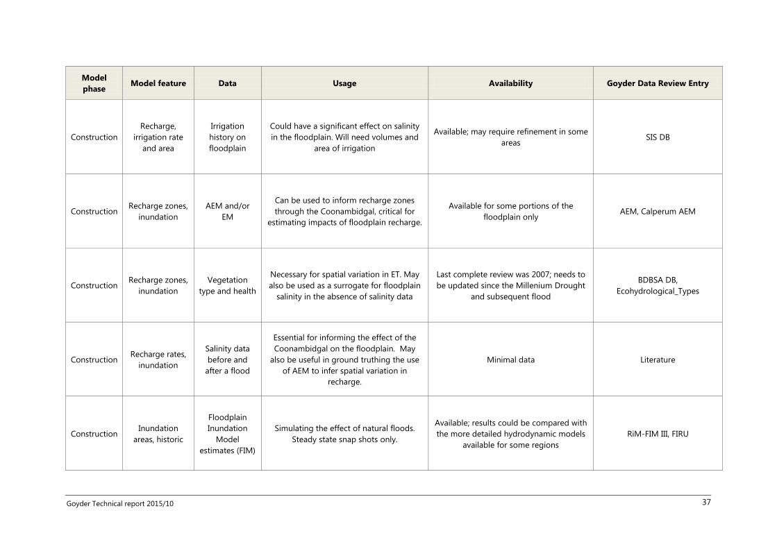
Goyder Technical report 2015/10 37
Model
phase Model feature Data Usage Availability Goyder Data Review Entry
Construction
Recharge,
irrigation rate
and area
Irrigation
history on
floodplain
Could have a significant effect on salinity
in the floodplain. Will need volumes and
area of irrigation
Available; may require refinement in some
areas SIS DB
Construction Recharge zones,
inundation
AEM and/or
EM
Can be used to inform recharge zones
through the Coonambidgal, critical for
estimating impacts of floodplain recharge.
Available for some portions of the
floodplain only AEM, Calperum AEM
Construction Recharge zones,
inundation
Vegetation
type and health
Necessary for spatial variation in ET. May
also be used as a surrogate for floodplain
salinity in the absence of salinity data
Last complete review was 2007; needs to
be updated since the Millenium Drought
and subsequent flood
BDBSA DB,
Ecohydrological_Types
Construction Recharge rates,
inundation
Salinity data
before and
after a flood
Essential for informing the effect of the
Coonambidgal on the floodplain. May
also be useful in ground truthing the use
of AEM to infer spatial variation in
recharge.
Minimal data Literature
Construction Inundation
areas, historic
Floodplain
Inundation
Model
estimates (FIM)
Simulating the effect of natural floods.
Steady state snap shots only.
Available; results could be compared with
the more detailed hydrodynamic models
available for some regions
RiM-FIM III, FIRU

Goyder Technical report 2015/10 38
Model
phase Model feature Data Usage Availability Goyder Data Review Entry
Construction ET rate,
potential
Monthly
potential ET
from BoM
Essential for evapoartion from surface
water bodies and ET Available BoM, CMRSET
Construction ET extinction
depth Root depth?
Possible from spatial distribution of
vegetation types/classes Needs to be developed
BDBSA DB,
Ecohydrological_Types
Construction ET rate curve
with depth
Ecological
literature?
Will inform the function used to describe
ET behaviour. Most recent literatue
suggests that an exponential function be
used
Needs to be developed Literature
Construction River Murray
levels, historic
River levels at
Locks
Informs heads for internal boundary
conditions for floodplain models. Ideal
temporal scale monthly or less.
Available Surface Water Data DB, Hydstra
DB
Construction River Murray
levels, historic
Backwater
curves
Informs heads for internal boundary
conditions for floodplain models. Available for the main channel
Surface Water Data DB, Hydstra
DB

Goyder Technical report 2015/10 39
Model
phase Model feature Data Usage Availability Goyder Data Review Entry
Construction
River Murray
bed
conductance
Heat tracers?
Other
technique?
Essential for internal boundary conditions
where ground and surface water interact. Minimal data
Literature, Calperum Flush
zones
Construction Anabranch
levels, historic
Any
observations?
Informs heads for internal boundary
conditions for floodplain models. Minimal data
Surface Water Data DB, Hydstra
DB (maybe)
Construction Anabranch bed
conductance
Heat tracers?
Other
technique?
Essential for internal boundary conditions
where ground and surface water interact. Minimal data Literature
Construction
Coonambidgal
hydraulic
conductivity
Laboratory
tests?
Necessary if modeling the Coonambidgal
explicitly. Also necessary if incorporating
its effect into ET or flood inundation
models.
Minimal data; some for Bookpurnong and
Chowilla Literature
Construction
Monoman
hydraulic
conductivity
Aquifer tests Necessary as a model input parameter.
Could be calibrated as well. Few aquifer test results
Waterconnect DB, SA Geodata
DB, SARIGDB?, SIS DB

Goyder Technical report 2015/10 40
Model
phase Model feature Data Usage Availability Goyder Data Review Entry
Construction
Monoman
hydraulic
conductivity
Texture from
borelogs Texture indicates the heterogeneity Available for a few locations only SIS DB
Construction Coonambidgal
porosity
Laboratory
tests?
Necessary as a model input parameter.
Need to know if there is change to the
porosity when inundated. Will cause a
significant change to the hydraulics on the
floodplain if it does.
Minimal data SA Soils DB, Literature
Construction Monoman
specific yield Aquifer tests Necessary as a model input parameter. Few aquifer test results
Waterconnect DB, SA Geodata
DB, SARIGDB, SIS DB
Construction Monoman
porosity
Laboratory
tests? Necessary for solute transport simulation Minimal data SA Soils DB; Literature
Construction Monoman
storativity Aquifer tests
Essential groundwater model input
parameter. Few aquifer test results SIS DB; Literature

Goyder Technical report 2015/10 41
Model
phase Model feature Data Usage Availability Goyder Data Review Entry
Construction
Underlying
aquitard vertical
hydraulic
conductivity
Aquifer tests
Essential groundwater model input
parameter. May be a calibrated parameter.
Has a significant effect on the flow
dynamic (i.e. lateral vs. vertical) in the
floodplain. Best if known to within an
order of magnitude.
Few aquifer test results SIS DB; Literature
Construction Dispersivity,
Monoman
Textbook
values? Necessary for solute transport simulation Minimal data Literature
Construction Salinity,
groundwater
Salinographs
from the
Monoman
Formation
Necessary for solute transport simulation Few floodplain bores in most areas. Waterconnect DB
Construction Salinity,
groundwater
Salinity with
depth,
Monoman
Formation
Can be used as a calibration target in a
floodplain salt model. Also can be used to
calibrate an AEM survey.
Minimal data Literature
Construction Salinity,
groundwater
AEM and/or
EM
Useful when modeling salt on the
floodplain explicitly. Could be used for
initial conditions depending on timing of
survey
Available for some portions of the
floodplain only AEM, Calperum AEM

Goyder Technical report 2015/10 42
Model
phase Model feature Data Usage Availability Goyder Data Review Entry
Construction Salinity, initial AEM
Could be used for initial conditions to
provide spatial variation to the salt
concentration on the floodplain depends
on timing of survey
Available for some portions of the
floodplain only AEM, Calperum AEM
Construction SIS Locations and
pumping rates
Essential input for groundwater models
due to significant effect on flux to the
floodplain and river
Available; seek regular updates from SA
Water SIS DB
Construction Salinity,
groundwater
Texture,
salinity,
moisture in
upper soil
profiles, depth
to water
Can be used as a calibration target in a
floodplain salt model. Also can be used to
calibrate an AEM survey.
Available across SA floodplain; CSIRO
smb://144.110.3.110/clw-
share9/floodpl/Floodplain_SA_field_results
FIP Soil Profiles
Calibration Potentiometric
head, Monoman Hydrographs
Useful groundwater models as both
calibration targets and initial conditions Few floodplain bores in most areas.
Waterconnect DB, Surface
Water Data DB, Hydstra
Calibration ET rate
Satellite data of
ET, spatial,
monthly
Large component of the floodplain water
balance so spatial variability and accuracy
important.
Coarse data available; finer resolution
should be developed CMRSET

Goyder Technical report 2015/10 43
Model
phase Model feature Data Usage Availability Goyder Data Review Entry
Calibration ET rate Field
observations
Eddy Covariance Flux Towers are best used
in conjunction with satellite-derived ET.
Other field based measurements may be
useful to observe daily/seasonal variation.
Available 2010-current Calperum Flux Tower
Calibration ET rate
Water balance
plots, soil
profiles, water
potentials
Can be used as a calibration target in a
floodplain salt model. Also can be used to
calibrate an AEM survey.
Available; 2005, 2007-2008 Bookpurnong Floodplain Pilot
Project
Calibration Gaining/losing
river
NanoTEM,
main river
channel
Useful for indicating sections of a reach
that are gaining and/or losing. Can be
used to check hydraulics in a numerical
model. May also be indicative of the bed
hydraulic conductivity.
Available for 2004 and 2012 NanoTEM
Calibration Gaining/losing
anabranches
NanoTEM,
anabranches
Useful for indicating sections of a reach
that are gaining and/or losing. Can be
used to check hydraulics in a numerical
model. May also be indicative of the bed
hydraulic conductivity.
Available for some anabranches NanoTEM
Calibration Salt load to
River Murray Run of River
Effectively base flow conditions and may
indicate reaches that are significant salt
contributors.
Available Salinity Register Models DB

Goyder Technical report 2015/10 44
Model
phase Model feature Data Usage Availability Goyder Data Review Entry
Calibration
Salt load to
River Murray
and
anabranches
Toroidal coil
salinity
Useful for indicating salinity contributions
from anabranches. Also used to partition
flood salt load contributions from specific
floodplains (AWE & CMC 2012)
Available in recent years Waterconnect DB
Calibration Salinity
distribution
AEM and/or
EM See Salinity, groundwater Available AEM, Calperum AEM
Calibration Salinity
distribution
Groundwater
salinity with
depth
See Salinity, groundwater Available AEM, Calperum AEM
Calibration Salinity
distribution
Changes in
vegetation
health
Indicates where has salinity has changed;
part of calibration confirmation Available (2002, 2007, 2009 surveys)
TreeHealth,
TreeHealth2007Katarapko,
TreeHealth2009RiverlandRamsar
Calibration Recharge
distribution
Geochemical
estimates of
recharge
Useful for freshwater lens history and for
constraining model recharge
Part of ARC Linkage study of freshwater
lenses Waterconnect DB? Literature.

Goyder Technical report 2015/10 45
Model
phase Model feature Data Usage Availability Goyder Data Review Entry
Scenarios River Murray
levels, future
Hydrodynamic
model
estimates
Hydrodynamic models provide better
temporal resolution for river stage levels
and inundated area which may affect
floodplain hydraulics and inundation
recharge
Available for Chowilla, Pike and Katfish RiM-FIM III, FIRU
Scenarios Anabranch
levels, future
Hydrodynamic
model
estimates
Available for Chowilla, Pike and Katfish RiM-FIM III, FIRU
Scenarios Inundation
areas, future
Hydrodynamic
model
estimates
Available for Chowilla, Pike and Katfish RiM-FIM III, FIRU
Scenarios SIS
Locations and
pumping
rates/target
levels
Essential input for groundwater models
due to significant effect on flux to the
floodplain and river
Available when SIS designed, SIS bores
and total pump volumes for
2011/12/13/14
SIS DB, SA_SIS_Interim16012014
Scenarios GCS
Locations and
pumping
rates/target
levels
Essential input for groundwater models
due to significant effect on flux to the
floodplain and river
Available when GCS designed

Goyder Technical report 2015/10 46
2.5 Discussion
2.5.1 Monitoring recommendations
Where a detailed model is required of an area’s floodplain salinity dynamics, the modelling should be supported
by a monitoring program. The scope of the program will depend on the aims of the project, budget and time.
Below is a list of monitoring tasks which would inform the modelling. For many of these items, there will be
existing data and infrastructure which should be reviewed before a monitoring plan is developed.
The monitoring program should consider:
Scout holes and bore logs to provide: thickness of the Coonambidgal Formation, thickness of the
Monoman Formation, thickness of the underlying aquitard (if present)
Observation wells in the Monoman Formation, monitoring potentiometric head and salinity
o some wells constructed so that salinity can be observed at different depths within the aquifer
Observation wells in the aquifer below the Monoman Formation monitoring potentiometric head, with
some initial sampling of salinity
Aquifer tests using the observation wells to determine the aquifer properties of the Monoman
Formation and the vertical conductivity (leakage) of the underlying aquitard
Observation wells in the regional watertable aquifer, near the floodplain edge, monitoring
potentiometric head, with some initial sampling of salinity
Aerial and/or land-based electromagnetic surveys, as these indicate the distribution of groundwater
salinity, both laterally and with depth
In-river transient electromagnetic (RTEM, also known as NanoTEM) geophysics surveys of anabranches
to determine where groundwater salt is entering the river
Monitoring of water and salinity levels in anabranches and wetlands to quantify storage and release of
salt
Surveys of vegetation type and health, as these indicate both current and past groundwater conditions.
For example, healthy trees will be found where they have access to freshwater from the surface water
system or groundwater, while dying trees indicate a change for the worse in access to freshwater.
Collate leaf area index (LAI) data; this can capture the nature of vegetation (type and health) and also
soil type (different vegetation types prefer different soils) and is derived from NDVI or LiDAR remote
sensing data
Gather data from weather stations based on the floodplain (particularly those on or near water)
monitoring rainfall and ET; these can be used to ground-truth remotely sensed estimates of AET (e.g.
CMRSET)
Laboratory and field analysis of the hydraulic properties of the Coonambidgal Formation
Consider whether an eddy covariance tower is required to groundtruth CMRSET satellite-derived
estimates of AET
Field estimates of riverbed, anabranch and wetland conductance. Expert opinion should be sought as to
the most appropriate method.

Goyder Technical report 2015/10 47
For areas where a detailed model needs to be calibrated against the results of a trial (e.g. artificial/environmental
watering trial or GCS trial, or possibly a natural flood), include the following at locations where changes in soil
and/or groundwater salinity are anticipated, before and after the trial:
Aerial, land-based and/or in-river electromagnetic surveys
soil salinity sampling
vegetation type and health survey
continuous logging of groundwater levels in key bores
To improve understanding of salinity dynamics in the study area, we recommend the following:
A review of observation well locations and the frequency of potentiometric head and salinity monitoring.
A review of existing AEM data, to identify and prioritise floodplain areas where: (i) no AEM data currently
exists, or (ii) significant changes in salinity are expected to have occurred since the last AEM survey.
Priority should be given to areas where new management works (such as regulators) are proposed.
2.5.2 Groundwater modelling priorities
The primary issues are of modelling method, scale (temporal and spatial), and data requirements. The priority
processes have been identified as follows:
1. Bank storage/river level change with solute transport. Investigate the:
a. Impact of stress period length on model outputs, particularly groundwater salt load to the
River.
b. Impact of using reservoir cells rather than river cells, due to their different interpolation over
time of river levels
c. Impact of fully simulating solute transport on salt load estimates, as compared to using flux
calculations multiplied by fixed salinity values
d. Impact of grid size
2. Evapotranspiration.
a. Compare the methods of representing ET as used in standard Salinity Register models, the
Chowilla model, the EM4 model and the Shahse River Valley model.
b. Compare the salt load estimates made when ET is constant versus when ET varies seasonally.
c. Develop recommendations for modelling ET which depend on the desired level of accuracy and
data availability.
3. Floodplain inundation recharge.
a. Compare the methods of representing inundation recharge used in the Chowilla model, the
EM4 model and the Murtho SIS climate sequence model.
b. Determine impact of spatial and temporal discretisation
c. Develop recommendations for modelling inundation recharge which depend on the desired
level of accuracy and data availability.

Goyder Technical report 2015/10 48
4. Density-dependence. Develop a cross-sectional model to investigate the importance of density in
simulating the interface between fresh river water and saline groundwater, i.e. the extent of a freshwater
lens. The model will require a code capable of simulating variable-density flow and solute transport.
The first three processes are investigated using numerical models in Chapter 4. The fourth process is being
investigated in the ARC-Linkage project, Dynamics and management of riverine freshwater lenses, a collaboration
between Flinders University, Monash University and DEWNR.

Goyder Technical report 2015/10 49
3 Surface water modeling approaches
Peter Cook
3.1 Introduction
There are a very large number of models that have been constructed for simulating river flow, and the interaction
between rivers and their floodplains. These models can be divided into two broad groups – hydrodynamic models
and hydrologic models. In general, hydrodynamic models solve differential equations for conservation of mass
and momentum. They model flow in terms of physical characteristics of the river (such as roughness coefficients).
Hydrologic models use a routing approach based on rating curves to simulate flow using a conceptual reservoir
approach.
This chapter gives a general overview of some of the most common surface water models (with an emphasis on
those models that have been applied in Australia), and a description of their functionality for representing
wetland and river floodplain systems.
3.2 Hydrodynamic Models
There are a large number of hydrodynamic river models, many of which have been used in Australia. For
predicting inundation of river floodplains, three different approaches are possible. In increasing order of
complexity, these are:
1. Quasi 2D Approaches based on 1D Hydrodynamic Modelling
2. Combination of 1D Hydrodynamic Model with a 2D Floodplain Reservoir Model
3. Full 2D Hydrodynamic Modelling
3.2.1 1D and Quasi 2D Hydrodynamic Approaches
The one-dimensional Saint-Venant equation for shallow surface water flow can be written:
1f o
h u u uS S
x g x g t
(3-1)
where Sf is the friction slope, S0 is bed slope, u is velocity, g is gravitational acceleration, x is distance and t is time.
The terms on the right hand side of Equation 3-1 represent bedslope, local inertia (or acceleration), advective
inertia, and pressure differential terms. Often simplifications to these equations are used that neglect different
terms to reduce computational complexity. Thus the diffusive wave approximation neglects the last two terms,
and the kinematic wave approximation neglects the last term.
Many river flow models rely on the one-dimensional solution to the Saint-Venant equation, or one of its simpler
approximations. Both HEC-RAS and MIKE 11 are examples of such models, and solve the full Saint Venant
equations for river flow using implicit finite difference schemes. To model the floodplains, a quasi two-
dimensional approach can be applied, in which the flooded areas are modelled as separate 1D river branches
(Figure 3-1). These are connected to the main river using spills or overflow structures that represent the
embankment elevations between the river bed and the floodplains. Thus, the floodplains are modelled by a
network of fictitious river branches and hydraulic structures. The details of the branching systems used by HEC-
RAS and MIKE11 are discussed in more detail by Villazon & Willems (2009). The approach requires that the
pathways across the floodplain are defined by the modeller in advance. Cross-sections perpendicular to these

Goyder Technical report 2015/10 50
flowpaths are derived from a digital elevation model (DEM), and roughness coefficients can be chosen to
represent the floodplain vegetation. Huang et al. (2007) describe the use of this approach using the DYNHYD
hydrodynamic model for simulating flooding due to breaching of dykes over a nine day period for a 50 km reach
of the Elbe River, Germany.
Figure 3-1 Quasi-2D approach to floodplain modelling, whereby the floodplain is simulated as branches of
the main river channel (Source: Huang et al., 2007).
3.2.2 1D Hydrodynamic River Model and 2D Floodplain Reservoir Model
A number of studies use a 1D hydrodynamic model for the main river channel, and a reservoir approach for the
river floodplain. One of the simpler such approaches is the model developed by Paiva et al. (2011). This approach
uses the full Saint Venant equations for 1D river flow and a simple storage model for the floodplain units. If the
water level in the river exceeds the height of the levee bank, then it spills over and inundates the floodplain.
Floodplain units are identified between river cross-sections, and water flows between the river and the floodplain
but cannot flow between adjacent floodplain units. Thus the water level for each floodplain unit is equal to the
water level in the main channel adjacent to the floodplain unit. Each floodplain unit is thus characterised by
simple water depth – flooded area relationship, and is hydrologically connected to a river segment. The model
was applied to the Purus River basin, one of the subbasins of the Amazon River. Floodplain width in Purus River
basin is approximately 30 km, and approximately 130 floodplain units were defined in the model (Figure 3-2). This
is a simple approach which focuses on water exchange between the river and the floodplain, rather than water
movement within the floodplain itself. The model thus does not represent floodplain hydrodynamics, but can
describe temporal patterns of floodplain inundation and the impact of floodplains on river hydrographs.
Other models use a grid-based approach for the floodplain. The advantage of this approach is that the pathway
of the flood on the floodplain is simulated in the model, and does not need to be pre-defined. One such model is
LISFLOOD-FP (Bates & De Roo, 2000; Wilson et al., 2007), which represents channel flow using the kinematic wave
approximation to the full 1D St Venant Equations, and floodplain flows using a reservoir approach implemented
on a raster grid. The model assumes that flow between floodplain cells, and between the river and floodplain
cells, is simply a function of the difference in free surface water height between those cells. Thus the dimension,
elevation and friction coefficient for each floodplain cell is defined. Each cell is treated as a storage volume, and
water can flow in any direction across the floodplain according to the water surface gradient and the local
topography. Manning’s Equation is used to calculate the flow rate between floodplain cells in each time step of
the model, and the roughness parameter can be adjusted depending upon the type of vegetation cover on the
floodplain.
Bates & De Roo (2000) present an example of the application of the LISFLOOD-FP model to the River Meuse, on
the border between The Netherlands and Belgium. The model covered a 35 km reach of the river, and had 9,639
nodes and 18,939 elements, and was run for a 21 day period to capture inundation from large flood. The model
described by Bates & De Roo (200) did not include direct precipitation onto the floodplain or runoff from upland
areas, or floodplain losses due to evapotranspiration and infiltration, although these could be readily added.

Goyder Technical report 2015/10 51
Subsequently, Wilson et al. (2007) presented an application of the LISFLOOD-FP model to a 13,000 km2 section of
the central Amazon floodplain, Brazil.
Figure 3-2 Location of river reaches, cross-section and floodplain units (grey shaded regions) on the Purus
River Basin, Brazil (Source: Paiva et al., 2011).
Figure 3-3 Wetting and drying process of floodplain elements of the raster model of Paz et al. (2011). Zf is
floodplain elevation, Za is water level, ha is surface water depth, hsub is water depth of soil reservoir, hres is
the available volume of soil reservoir, which has a maximum capacity equal to Hsmax.

Goyder Technical report 2015/10 52
Paz et al. (2011) use a similar approach to examine floodplain inundation in the Upper Paraguay River Basin. The
authors coupled the 1D hydrodynamic model IPH4 with a floodplain raster model based on the LISFLOOD-FP
approach. However, the authors approach differed from the LISFLOOD-FP model in that flow between floodplain
elements was based upon flow through channels, whose width and length could be specified and was not related
to the floodplain element grid size. The model also included a vertical water balance for the floodplain cells.
Surface water only occurred on the floodplain when the soil moisture storage was exceeded. Input to the soil
moisture storage occurred by flow from adjacent floodplain units and as precipitation. Loss occurs by surface
flows and by evapotranspiration, with the evapotranspiration rate dependent upon the soil moisture storage
(Figure 3-3).
3.2.3 Full 2D Hydrodynamic Approaches
River flows across floodplains can also be simulated using full two-dimensional solution to the river
hydrodynamic equations. MIKE 21 is one such program. Variables are defined across a grid, and the model solves
the full time-dependent non-linear equations of continuity and conservation of momentum. MIKE 21 can be used
for simulation of water flow in rivers, lakes, estuaries and coastal areas, as well as across floodplains. Infiltration on
the floodplain can also be simulated using the MIKE 21 HD Infiltration and Leakage module. The MIKE FLOOD
model dynamically couples the one-dimensional MIKE11 river model and the two-dimensional MIKE21 model by
defining linkages between the two models that allow water to move between the 1D and 2D domains.
Critical data for the use of such models is a digital elevation model with sufficient horizontal and vertical
resolution to capture the important topographic features of the floodplain. Model calibration is usually achieved
by adjusting channel and floodplain roughness coefficients, and sometimes also adjusting cross-section and
topographic data, to reproduce recorded hydrographs and observations of floodplain inundation (Wen et al.,
2013). The main advantage of the 2D approach is that it provides velocities and discharges in 2 dimensions. The
path of the floodwave is determined from topographic information, and does not need to be specified a priori.
Tuteja & Shaikh (2009) used the MIKE FLOOD model to simulate surface flows across the Koondrook-Perricoota
Forest to support development of environmental watering plans and engineering design of structural works, and
also compared results from the MIKE FLOOD model (which combines 1D and 2D approaches) with results of
Quasi-2D and 2D approaches. The Koondrook-Perricoota Forest covers an area of 337 km2, and is located north
of the River Murray floodplain between Torrumbarry Weir and Barham. The 2D MIKE 21 model used a grid
resolution of 40 m. However, a comprehensive MIKE 11 model was developed at a fine resolution to capture
inundation dynamics and flow exchange between channels and the floodplains, which could not be adequately
represented by the MIKE 21 floodplain model alone. Thus six floodplain channels were delineated, using 809
cross-sections up to 200 m width and described at 1 m intervals. The models were validated using remote sensing
mapping of inundation areas for 12 images across three historical events (1991, 1993 and 2000), and also
mapped flood extents for the 1946 flood. The authors noted that without including the floodplain channels, the
2D floodplain MIKE 21 model overestimated inundation extent, whereas the Quasi 2D MIKE 11 model
underestimated inundation extent, as observed in satellite imagery and historical records. The authors also
observed that inundation extent had a hysteretic relationship with river flow (Figure 3-4), which reflects water
trapped on the floodplain following peak river flows. The hysteretic relationship was not predicted by the Quasi
2D MIKE 11 model.

Goyder Technical report 2015/10 53
Figure 3-4 Hysteretic relationship between river flow rate and floodplain inundation area, observed for
the Koondrook Perricoota Forest. Inundation area is higher for the same river flow rate on the falling limb
of the flood (Source: Tuteja & Shaikh, 2009).
Chen et al. (2012) used the MIKE FLOOD model to simulate a 500 km2 portion of the Florida Everglades using 400
m x 400 m grid cell, to simulate both flow and solute transport using the conservative chloride ion. They noted
that although the 400 m grid resolution was the best topographic resolution available, it was still too coarse to
capture some of the topographic features that control shallow water flows. They also noted that the ability to
define depth-dependent roughness is important for chloride transport simulations, and this that capability is not
currently available in MIKE21.
3.2.4 Hydrologic Models
River reservoir models use a hydrologic routing approach to calculate flow. Most of these models consider the
river as a series of nodes connected by links. Nodes are points on the river system that have certain operation or
physical processes associated with them. These include gauges, tributary of pumped inflow locations, on-river
storages, diversion points and pumps, wetlands and floodplain detention storages. Water flow and water quality
routing occurs along links which separate the nodes (Simons et al., 1996).
Hydrologic routing relies on the continuity equation. In its simplest form, inflow to the river reach is equal to the
outflow of the reach plus the change in storage.
( ) ( )
SI t O t
t
(3-2)
where I is the inflow to the reach during, O is outflow from the reach; and S is the water storage in the reach.
Reservoir models have the advantage of small computational times, and so they are suitable for inclusion in
decision support systems, and for optimisations and uncertainty analysis, which require many model runs. This
type of model is widely used for river management in Australia, and examples include BIGMOD, REALM, IQQM
and Source.

Goyder Technical report 2015/10 54
The MDBA uses MSM-BIGMOD to model river flow and salinity. The model (Close, 1996; MDBC, 1996, 2002) is
specific to the River Murray system, which is represented as a number of river reaches and branches. MSM is a
monthly simulation model used for modelling flows, operating rules and irrigation demands, and BIGMOD is a
daily flow routing and salinity model that extends from Hume Dam to the barrages at the Murray Mouth.
BIGMOD uses a water balance approach, with the downstream flow of each reach calculated as:
out in hf emq q S d E A L L (3-3)
where qout is the flow out of the reach, qin is flow into the reach, ∆S is the change in reach storage, d is the
distributed diversion, E is the net evaporation rate, A is the reach surface area, Lhf is the high flow losses and Lcm is
the continuous monthly losses. The storage in each reach is a function of the flow rate, which is contained with a
lookup table. A second lookup table contains the relationship between flow rate and travel time for each reach
(Rassam and Werner, 2008).
BIGMOD has been widely used for modelling salinity within the River Murray, and salinity within the model is
calculated based on the water balance. Salinity values are assigned to different particles of water, and their
movement is tracked through the model. Lakes are assumed to be fully mixed, and weirs may either be assumed
to be fully mixed, or can be simulated as part of the river. Salt loads from tributaries and drains are included in
the model, and increases in salinity can also occur due to evaporation, with decreases in salinity due to dilution
from precipitation or inflow of water having lower salinity. The model minimises the difference between simulated
and observed salt concentration in the river by introducing an unaccounted salt inflow. (Negative values indicates
salt outflow.) Unaccounted salt inflow accounts for processes that are not explicitly simulated in the model
(including groundwater inflows), as well as errors introduced by the various model assumptions and
simplifications. Telfer et al. (2012) describe application of the BIGMOD hydrologic model to simulate salinity
within the lower River Murray system. The model simulates both flow and salinity, with excellent fits to
observation data (Figure 3-5). However, very high unaccounted salt inflows are required, representing 35% of the
total salt loads to the river reach from Euston to Morgan over the 39 year period from July 1970 to June 2009. The
unaccounted salt inflows are thought to be derived almost entirely from floodplain sources (Telfer et al., 2012).
REALM and IQQM are river hydrology models developed to simulate the operation and optimisation of water
supply systems. REALM is widely used in Victoria and supported by the Victorian Department of Sustainability and
Environment (DSE), wheras IQQM is preferred in New South Wales. Both models use a node-link approach, and
are able to represent a wide range of river features and operating rules. Mass balance calculations are applied for
off-river storages and wetlands. In particular, IQQM simulates the floodplain as a series of reservoirs (or cells),
each with its own specific depth – area – volume relationship. A water balance is performed for each wetland, with
change in storage equal to the difference between inflows and outflows. Inflows occur due to surface water flows
from adjacent wetlands or from the river, and outflows occur due to evaporation and surface water flows to
adjacent areas. A storage can have inflows and outflows from and to multiple locations, to reflect the complexity
of floodplain topography. Direction of flow on the floodplain can change depending on the size and nature of
inundation extent. In the case of two adjacent cells, flow direction can vary depending upon which cell gets
inundated first.
Source simulates river systems in a similar manner to IQQM, but includes some additional functionality to
represent some simple surface water – groundwater interactions (Welsh et al., 2012). In particular, the impacts of
groundwater pumping and recharge on river – aquifer exchange are included. Simple analytical expressions are
used to estimate the time delay between groundwater pumping and flow to the river, based on the distance of
the bore to the river, and the aquifer diffusivity (Rassam et al., 2009). However, the model does not simulate salt
transport directly. Rather, the salinity is defined by the user, and the model calculates salt loads to the river by
multiplying the groundwater flow rate by the specified salinity.

Goyder Technical report 2015/10 55
Figure 3-5 Comparison of BIGMOD simulated salinity at Morgan with observation data for the period 1975
– 1999 (Source: Telfer et al., 2012).
3.3 Combining Hydrodynamic and Hydrologic Models
A number of studies have attempted to combine the more accurate simulation of hydrodynamic models with the
run-time advantage of hydrologic models. The principle of this approach is to use the hydrodynamic models to
develop relationships between flow and inundation, and to embed this relationship into a hydrologic model. For
example, Mackay et al. (2011) used the MIKE 21 2D hydrodynamic model to determine the relationship between
flow and inundation for a section of the Lower Murrumbidgee River centred on Yanga National Park, near
Balranald, NSW, and used this relationship in an IQQM model. The hydrodynamic model involved a grid size of 20
m to simulate an area of approximately 300 km2. (Comparisons were also made with a hydrodynamic model using
a coarser 80 m grid cell; Figure 3-7) Based on results of the hydrodynamic simulations, the floodplain area was
split up into 38 cells, each with its own water level – discharge relationship (derived from the hydrodynamic
model). Water level – discharge relationships were derived for boundaries between all reservoirs, and between
the reservoir and the river. Many cells had multiple inflow and outflow points, reflecting the complexity of the
floodplain topography. Direction of flow on the floodplain can change depending on the size and nature of
inundation extent. In the case of two adjacent cells, flow direction can vary depending upon which cell gets
inundated first. Following calibration, the results of the IQQM model were compared with inundation extent
mapped using satellite data obtained at 84 discrete time intervals within the period 1988-2006. Although there
were strong correlations between mapped and observed inundation extent, the modelled inundation extent was
consistently lower than observed extent (Figure 3-6). It was found that modelled results better matched observed
results for larger floods than for smaller flood events. (The modelled inundation area is averages 79% of the
observed inundation area in wet years, but only 44% during drier periods.) Areas that were poorly simulated
included those that received flows from other areas of the floodplain, rather than directly from the river.

Goyder Technical report 2015/10 56
Figure 3-6 Relationship between modelled and observed inundation extent in a section of the
Murrumbidgee River floodplain, Yanga National Park, NSW (Source: Mackay et al., 2011).
Figure 3-7 Comparison of the effect of grid cell size on simulation of inundation extent of the
Murrumbidgee River in Yanga National Park, NSW using a hydrodynamic model. Simulated floodplain
inundation is much greater using a 20 m grid cell (blue areas) than using a coarser 80 m grid (red and

Goyder Technical report 2015/10 57
purple areas). (Purple areas are inundated in both models, and green areas are uninundated.) (Source:
Mackay et al., 2011).
A similar approach was used by Wen et al. (2013). These authors developed a spatially distributed 2D
hydrodynamic model for the Macquarie Marshes using the MIKE FLOOD modelling system, and then used this to
prepare IQQM hydrologic model. The hydrodynamic model included almost 500 km of river channels (simulated
in MIKE 11), and 213443 active cells across the floodplain (simulated in MIKE 21). The MIKE FLOOD model was
calibrated against six historic flow events, covering the full range of flow conditions in the marshes. The complex
relationships between flow and inundation apparent from the hydrodynamic model were then simulated with an
IQQM model with 36 storages to represent key wetlands, and a total of 88 inflow pathways to these wetlands. In
IQQM the inflow to each wetland is determined by the river level (or level of another wetland), and this
relationship was derived from the MIKE FLOOD model. The model was used to simulate effect of water extraction
for irrigation on marsh inundation.
3.4 Discussion
The choice of simulation model should be based on an assessment of the key processes that need to be
represented to produce accurate predictions. However, it is also often influenced by practical considerations, such
as model run time. Wen et al. (2013) note that long model run times is the main impediment to the widespread
use of 1D and 2D hydrodynamic models for river and floodplain simulation. Such models often take hours to days
for single simulations, depending on the size of the modelled area, and time period of the simulation and the
spatial and temporal discretisation. For example, Chen et al. (2012) report that MIKE FLOOD modelling of the
Florida Everglades took 70 minutes for one year simulation (on 2.83 GHz Intel® Core(TM)2 Quad CPU), while the
LISFLOOD-FP hydrodynamic model of the Amazon wetlands described by Wilson et al. (2007) took 14 days to run
(3.0 GHz PC). Tuteja and Shaikh (2009) report simulation times of 15-30 minutes for quasi 2D MIKE 11 modelling,
5 – 15 days for 2D MIKE 21 modelling and up to 50 days for combined 1D and 2D MIKE FLOOD modelling of the
Koondrook Perricoota Forest wetlands (Intel Dual-Core PC with 2.13 GHz processor speed and 3.25 GB RAM).
These longer run times can become prohibitive if models are to be incorporated into decision support systems or
used for uncertainty analysis, both of which can require large numbers of model runs. Run time can be reduced
by increasing model cell size, although this can affect model results. If the grid cells are too large, the model will
not accurately simulate smaller floods that inundate only parts of the floodplain. Reservoir models have much
faster run times which allow them to be used in decision support systems and for assessment of multiple
management options. Thus Mackay et al. (2011) report an IQQM runtime for 100 year simulation at daily time
scale of only a few minutes. The longer run times of the hydrodynamic models also means that it is more difficult
to apply these at larger spatial scales, and this is the area where the simpler hydrologic models have their main
advantage.
When using simple models, it is important to understand the assumptions behind them, and consequent errors
that can arise when these assumptions do not hold. The historic driver for many of the hydrologic models (e.g.,
IQQM, REALM) has been the need to manage water allocation and water use associated with irrigation and town
supply (Hameed and Podger, 2001). They were not explicitly designed for management of environmental flows,
and so wetlands were either not represented, or represented so coarsely as to be of little value for simulating
floodplain processes (Wen et al., 2013). However, these models are now being used to simulate floodplain
inundation, and so their accuracy for this purpose needs to be assessed. Examination of the BIGMOD simulation
of lower River Murray salinity reveals that a large fraction of the salt loads into the model are unaccounted salt
inflows, which are essentially a statistical calibration parameter to represent processes that are not explicitly
simulated by the model. The model would therefore not be capable of simulating changes to the processes
affecting this salt inflow.
The Source model has recently been modified to include changes in groundwater flow to the river due to
irrigation (an increase in groundwater flow to the river) or groundwater pumping (which results in a decrease in
groundwater flow to the river). Salt loads are calculated by multiplying the groundwater inflow to the river by a
salinity, which is specified by the user. Thus changes in salt loads to the river due to groundwater pumping or

Goyder Technical report 2015/10 58
irrigation are assumed to be proportional to the change in groundwater flow rate. The model does not simulate
salt transport directly, and so cannot simulate changes in the concentration of groundwater discharging to the
river. However, it is likely that temporal changes in concentration of groundwater discharging to the river occur
due to processes within the floodplain, although the magnitude and significance of these is not yet clear. Thus
flooding of floodplain areas may lead to infiltration of relatively fresh groundwater, which would ultimately
discharge to the river. In between floods, evaporation within the floodplain environment would concentrate salt,
increasing concentrations in the groundwater. Thus the concentration of groundwater discharging to the river
may vary in time depending on the flooding history. None of the current models can simulate this process, even
in a rudimentary form. Although many of the available hydrologic and hydrodynamic surface water models are
also able to simulate water quality (and in particular, salinity), and a few contain simple groundwater flow
representations, none of them are able to simulate leaching of salts beneath the base of floodplains or wetlands,
and the subsequent transport of that salt back into the river. Of course, the importance of these concentration
changes is currently unclear, and analysis of the significance of these processes would be valuable.
Comparison between predictions of simple models and more complex models should precede the decision to use
simple models, but this important step is frequently overlooked. Simple models simplify or omit certain flow or
transport processes, and will be in error if these processes are important. Simpler models also have lower data
requirements than complex models. However, even if the data required by the complex models is not available, it
is still possible to carry out sensitivity analysis for these unknown parameters using the complex models. This
allows the effect of the unknown (or poorly known) parameters on model predictions to be determined. This is
not possible using simple models, and so the effect of simplifying assumptions often cannot be explicitly
determined.
The data required to construct accurate hydrodynamic models of river floodplain and wetland systems includes
surface elevations on a fine resolution across the entire floodplain area, and information on hydraulic properties
(e.g., surface roughness). Within recent years, the availability of accurate digital elevation models has increased,
so that surface elevation data is now often available with a spatial resolution of a few tens of metres and vertical
accuracy of 1 – 2 m. Higher resolution is available using LiDAR systems. Surface roughness data is often obtained
using literature values that relate it to vegetation type and density, but also used as a calibration parameter.
Hydrologic models determine inundation and flooding using volume – area relationships and relationships
between river and wetland level and flow rates between river and wetland (and between individual wetlands or
floodplain elements). Spatially explicit information on precipitation, evaporation and infiltration for the floodplain
is also required where these components are included in the models. However, observations of water level and
discharge and spatially infrequent – flow gauges are usually restricted to the main river channel, and even water
level data is often absent across large floodplain areas. Remote sensing observations of inundation extent do not
completely fill this void, and they are often limited in spatial resolution and temporal coverage (Schumann et al.,
2009). One option is to develop a 2D hydrodynamic model with high spatial resolution to simulate inundation,
and to use the relationships derived from this for hydrodynamic models. When this approach is used, the
calibration of the hydrologic models can only be guaranteed for the range of river flood levels simulated using
the hydrodynamic model from which it was derived.

Goyder Technical report 2015/10 59
4 Groundwater model trials
Virginia Riches, Tariq Laattoe, Juliette Woods & Carl Purczel
The aim is to simulate key floodplain processes and drivers using MODFLOW in a simplified model of the SA River
Murray floodplain. Numerical experiments are performed to explore how process representation affects model
outputs. As such, the model is a “generic model” according to the model classification discussion of the National
Water Commission Groundwater Modelling Guidelines (Barnett et al., 2012):
“These models are developed primarily to understand flow processes and not to provide quantitative
outcomes for any particular aquifer or physical location. They can be considered to provide a high level
of confidence as their accuracy is only limited by the ability of the governing equations to replicate the
physical processes of interest. While they provide high confidence when applied in a general, non-
specific sense, if the results are applied to or assumed to represent a specific site the confidence level
will automatically decrease.”
Generic models are a special case and cannot be easily matched to the Confidence Level Classification of Barnett
et al. (2012).
The primary issues are of modelling method, scale (temporal and spatial), and data requirements. Both
groundwater flow and solute transport are simulated. Base case models are developed, simulating a variety of
floodplain conditions where processes and drivers are constant over time. River level, ET, and groundwater
recharge are homogeneous and do not vary over time. The base case models are calibrated to match reasonable
ranges of groundwater flux to the floodplain, groundwater salt load to the river, and actual ET.
Once the base case models are satisfactory, they are modified to simulate scenarios in which drivers vary over
time. Different parameters and process representations are trialled. The priority processes are:
1. River level change. A MODFLOW/MT3DMS model tests the following, without simulating floodplain
inundation:
a. Impact of temporal discretisation of changes in river level on model outputs, particularly
groundwater salt load to the River.
b. Impact of using reservoir cells rather than river cells, due to their different interpolation over
time of river levels.
c. Impact of fully simulating solute transport on salt load estimates, as compared to using flux
calculations multiplied by fixed salinity values.
d. Impact of grid size.
2. Evapotranspiration. Develop a MODFLOW model to investigate the following:
a. Impact of temporal discretisation of changes in PET on model outputs, particularly ET flux and
river conditions.
b. Sensitivity to ET parameters.
c. Impact of spatial variations in ET.
d. Impact of the shape of the ET function with respect to depth to water.
3. Floodplain inundation recharge. Develop a MODFLOW model to do the following:
a. Compare the impact of floods with and without inundation.
b. Consider the impact of a wetland (backwater) on floodplain dynamics

Goyder Technical report 2015/10 60
The results of the numerical experiments are used to develop recommendations for the simulation of floodplain
salinity processes in the SA MDB.
4.1 Model Conceptualisation
The Goyder Floodplain Model has been designed to represent generic conditions for the SA River Murray
floodplain in the study area (Figure 4-1). However, a range of conditions exists (see the conceptual model
discussion in Woods, 2015a). For example, river conditions may be gaining, throughflow, or losing when the river
has low flow. The floodplain may or may not include a river lock (including a change in weir pool level due to the
construction of the lock). The floodplain may be narrow or wide, and the dominant direction of regional
groundwater flux may be lateral or vertical into the floodplain. For this reason, the Goyder Floodplain Model has
six bases cases representing a variety of conditions encountered in the study area. This is explained in greater
detail below.
Figure 4-1 Model study area
Hydrogeological parameters vary within the study area. The base case parameters are informed by an
amalgamation of data from this area, but are not specific to any one location. Where there is a wide range of
possible parameters, values from the Pike Floodplain have been adopted. Pike Floodplain was selected as it is
currently DEWNR’s highest priority for a numerical groundwater model, owing to the proposed regulator and
salinity management works.
Where there is uncertainty regarding how to simulate a process or driver, the base case and initial scenarios
adopt methods used by the Salinity Register models. The Salinity Register models are currently the most up-to-
date simulations of SA MDB groundwater processes but simulate floodplain processes extremely simply, hence
they provide a starting set of assumptions. It is anticipated that the Salinity Register models will be revised over
time to include improved representation of floodplain processes, based on this study and others.

Goyder Technical report 2015/10 61
The Salinity Register models do not simulate solute transport (Section 1.3.1). Instead, the flux of solute is
determined by assigning a set concentration, based on a background salinity value, to the gained river volume.
This approach is sufficient for Salinity Register purposes, to estimate long-term river salinity impacts from
changes on the highland, and the models have provided a reasonable match to observed salinity trends in the
River Murray. However, solute transport is required to capture short-term, localised salinity impacts on the
floodplain, such as those driven by environmental watering, natural flooding, floodplain pumping or weir-pool
manipulation. Solute transport is included in the Goyder Floodplain models to simulate variation both spatially
and temporally of the groundwater salinity distribution on the floodplain.
4.1.1 Hydrogeology
As the Goyder Floodplain Model is a generic SA MDB floodplain model, the hydrogeology represented in the
model is also generic. At many locations in the study area, the hydrogeology is significantly more varied and
complicated.
The hydrogeology of the floodplains in the lower River Murray is described in detail in Woods (2015a). Within the
incised river trench, sediments consist of the Monoman Formation (a semi-confined aquifer) overlain by the
Coonambidgal Formation (an aquitard). Beneath the Monoman Formation are the regional units: an aquitard such
as the Bookpurnong Formation and the regional aquifer system of the Murray Group (Figure 4-2). The edge of
floodplain (defined by the incised river trench) sits adjacent to a regional aquifer, either the Loxton Sands
Formation or the upper units of the Murray Group, depending on location. For the sake of simplicity, the regional
aquifer laterally adjacent to the floodplain aquifer is referred to as the Loxton Sands in this chapter; however, the
model results are likely to be similar for locations where this aquifer is the upper units of the Murray Group.
The Coonambidgal Formation consists predominately of clay sediments and is known to be of low hydraulic
conductivity at many locations along the lower River Murray. However, it is also fairly variable along the river
channel, ranging from low-permeability clays to sandy clays and clayey silts. It also has a varying thickness, from
absent to up to 10 m thick. The Coonambidgal Formation determines the unconfined to semi-confined nature of
the Monoman Formation.
In terms of floodplain processes, the Coonambidgal Formation is critical in determining how groundwater will
interact with surface processes, such as evapotranspiration, as well as how floodplain inundation becomes
groundwater recharge. It is also in direct connection with the river for much of the floodplain as well as other
surface water features.
The Monoman Formation is considered to be a semi-confined to unconfined aquifer consisting of clean fine to
coarse alluvial sands (Anon, 1989). The thickness of this aquifer also varies across the floodplain, in the order of 10
to 40 m. In some areas it is known to be in direct connection with the river. The salinity of this aquifer ranges from
5,000 to 70,000 mg/l (RPS Aquaterra, 2012).
The Goyder Floodplain Model has two topographic conceptualisations. The first conceptualisation focuses on the
incised river trench only (Figure 4-3 (a)) and includes a broad floodplain on either side of the river. The second
conceptualisation includes a highland area on one side of the river, with the river close to the edge of the
highland (Figure 4-3 (b)).
The Loxton Sands is a regional aquifer that sits on the highland adjacent to the Monoman Formation and
Coonambidgal Formation. It is also a semi-confined to unconfined aquifer consisting of fine to medium sands
with some clay and silt layers. The salinity of the Loxton Sands is similar to the Monoman Formation.
The regional aquitard, where present, separates the overlying Monoman/Loxton Sands and the underlying Murray
Group. For example, the Bookpurnong Formation consists of poorly consolidated silts and clays and can be up to
40 m thick.
The Murray Group is a regionally extensive confined aquifer of varying water quality. It consists of multiple
different formations, which vary in presence/absence throughout the floodplain. These formations also vary in

Goyder Technical report 2015/10 62
hydraulic properties, with some formations being better aquifers than others. This group can be in the order of
100 m thick, depending on location and has a salinity of approximately 20,000 mg/l (Sharley & Huggan, 1995).
As discussed in Woods (2015a), both floodplains and surface water features can be gaining, throughflow or
losing. The majority of floodplains in the study area would be considered gaining floodplains, where groundwater
flows into them.
Table 4-1 Hydraulic parameters from previous studiesprovides a summary of hydraulic parameters for these units
from previous studies and has been used to inform the parameters in the Goyder Floodplain Model.

Goyder Technical report 2015/10 63
Table 4-1 Hydraulic parameters from previous studies
Hydrogeological
Unit
Hydraulic conductivity
(m/day)
Tranmissivity
(m2/day)
Storage (-)
Source
Kh Kv T S(1)
Sy
Woorinen
Formation
- - - - -
Coonambidgal
Formation
- - - - -
Monoman
Formation
2 – 19 - - 4x10⁻⁴
- URS (2000)
REM (2002b)
REM (2002a)
25 - 33 - 500 – 655 5x10⁻³
- AWE (2012a)
AWE (2012b)
4.07 – 536 4.1.1.1.1.1 -
30 – 1800 7.06x10⁻⁷
–
6.47x10⁻²
4.1.1.1.1.2 -
AWE(2011)
Blanchetown Clay - 3x10⁻⁴
- - - REM (2002b)
Loxton Sand
0.3 – 5.8 - 26 – 121 2x10⁻⁴
–
2x10⁻³
0.06-0.13 REM (2002b)
REM (2002a)
REM (2005)
3 – 59 - 79 – 1470 5x10⁻⁶
–
0.275 4.1.1.1.1.3 -
AWE (2012a)
AWE (2012b)
2.59 – 33.4 4.1.1.1.1.4 -
41.5 – 421 2.45x10⁻⁸
–
2.96x10⁻¹
4.1.1.1.1.5 -
AWE(2011)
Lower Loxton Clay
and Shells
- - - - -
Bookpurnong
Formation
- 6x10⁻⁴
– 1.6 - - - REM (2002b)
REM (2002a)
Mu
rray G
rou
p L
imest
on
e
Pata
Formation
0.05 – 0.1 - - 1x10⁻³
(Ss) - REM (2002b)
0.09 – 0.72 1x10⁻³
–
6x10⁻³
4.1.1.1.1.6 -
3.12x10⁻⁵
–
4.91x10⁻⁴
4.1.1.1.1.7 -
AWE(2011)
Winnambool
Formation
- - - - -
Glenforslan
Formation
0.14 – 0.56 3x10⁻³
–
10x10-3
- 1.56x10⁻⁴
–
1.95x10⁻⁴
- AWE (2011)
Mannum
Formation
0.05 – 0.1 - - - - URS (2000)
1.25 – 2.56(2)
62x10-3
–
133x10-3(2)
4.1.1.1.1.8 -
1.48x10⁻⁴
–
2.75x10⁻⁴ (2)
4.1.1.1.1.9 -
AWE (2011)
(1) S is storage coefficient, which is the product of specific storage (1/m) and layer thickness (m), and is
hence dimensionless (2)
Upper Mannum Formation

Goyder Technical report 2015/10 64
Figure 4-2 Simplified Floodplain Hydrogeology

Goyder Technical report 2015/10 65
Figure 4-3 Goyder Floodplain Model Conceptualisation ((a): Broad Floodplain and (b): Broad Floodplain
plus Highland)
4.1.2 Surface Water
Surface water plays a key component in how floodplains behave and interact with the groundwater. Surface water
features are simulated simply within the Goyder Floodplain Model, consisting of the main river channel and a
wetland. The River Murray in the study area may have gaining, throughflow or losing conditions, hence it was
necessary to develop base cases which covered all these possibilities.
4.1.3 Base case conceptualisations
From the discussion above, it was identified that a minimum of three model conceptualisations needed to be
represented in the Goyder Floodplain Model. In addition to the three conceptualisations, the river needed to be
represented as both a river with a lock and a river without a lock. From these combinations, the base models
given in Table 4-2 were developed.
Table 4-2 Goyder Floodplain Model – Base Model Conceptualisations
Case Floodplain River Lock present
Case A – with Lock Gaining Losing Yes
Case A – without Lock Gaining Losing No
Case B – with Lock Gaining Throughflow Yes
Case B – without Lock Gaining Throughflow No
Case C – with Lock Gaining Gaining Yes
Case C – without Lock Gaining Gaining No

Goyder Technical report 2015/10 66
4.2 Base Model Construction, Validation and Initial Findings
4.2.1 Model code
The Goyder Floodplain model has been built in Groundwater Vistas Version 6. Initially, MODFLOW2000
(Harbaugh et al. 2000) was used to simulate groundwater flow, but this led to difficulties with re-wetting that
were resolved by switching to the MODFLOW2005 (Harbaugh, 2005) code using the NWT solver and UPW
package (Niswonger et al., 2005) (Section 4.2.8.2). MODFLOW-USG (Panday et al., 2013) was used to investigate
spatial discretisation of the model domain (Section 4.3.1.3). MODFLOW Surfact (Hydrogeologic, 1996) was used to
investigate re-wetting of the Coonambidgal Formation (Section 4.2.8.2). The NWT automate solver options was
set to moderate and the solver used a head change criteria of 10-5
m, a flux change criteria of 10 m3/day and
maximum outer iterations set to 100.
The MODFLOW-related solute transport code MT3DMS (Zheng & Wang, 1999) was used to simulate solute
transport for almost all flow scenarios. MT3DMS utilizes the flow fields generated during the MODFLOW
simulation to solve the advection-dispersion equation. MT3DMS utilizes an implicit formulation based on
generalized conjugate gradient (GCG) method to solve the dispersion and sink/source terms and a separate
solution scheme for the advection term selected by the user. All simulations utilized the inherently stable third-
order mass-conservative TVD (total variation diminishing) scheme to solve the advection term with the Courant
number criteria restricted to 0.75. The concentration closure criterion for convergence with the GCG solver was
set at 10-9
. Transport step sizes remain fixed for each simulation and are determined internally by the TVD
scheme, which avoids any potential solution oscillation during iteration as well as minimal numerical dispersion.
Sorption was excluded from all solute transport simulations.
4.2.2 Domain and Grid
The model domain for the Goyder Floodplain model is loosely based on the dimensions of the Pike Floodplain
and is 13 km long by 8 km wide. The cell size for the model is 125 m x 125 m, which was chosen based on the cell
sizes used in other models that cover the lower River Murray floodplain (notably the SA Salinity Register Models).
This resulted in a model with 64 rows and 104 columns with a total of 26,624 active cells over 4 layers.
The impact of cell size was investigated and is reported in Section 4.3.1.3.
4.2.3 Initial conditions and stress periods
Initial conditions for the base models set potentiometric head at top of surface, then ran until convergence at
steady state. The heads from the steady state model were then used as initial conditions for the scenario
modelling. Where the scenario changed a key parameter, such as evapotranspiration extinction depth, the base
models were re-run with this parameter change to create a new initial head for that scenario run.
Initial solute distributions for scenario models were obtained by running MT3DMS to a perceived steady state
using the steady state flow field from the relevant MODFLOW base simulation. A difference of less than 0.001% in
the salt flux to river for consecutive months was selected as the metric for perceived steady state.
Evapoconcentration was included in all simulations and resulting in greater concentrations of 35,000 mg/l on the
floodplain. To facilitate better comparison with the current method used to determine salt flux to river all
concentrations exceeding 25,000 mg/l in the Monoman Formation were reduced to 25,000 mg/l for the initial
solute distributions.
All the transient scenarios were run over a 20 year time period, nominally based on the period between 1/1/1992
and 31/12/2011. This time period was selected as it includes both a wet period with significant flooding as well as
an extended dry period. Where appropriate, data from this period has been incorporated into the model. Stress
period length depends on the scenario. Annual, monthly, or sub-monthly stress periods were used.

Goyder Technical report 2015/10 67
4.2.4 Model Layers
The Goyder Floodplain Model has four layers, in line with the hydrogeological conceptualisation outlined
previously (Figure 4-3). Layers 2 to 4 are consistent between model base cases, while layer 1 is consistent between
Cases A and B but modified in Case C.
4.2.4.1 Surface Elevation
The Goyder Floodplain Model, while being designed to represent floodplain conditions, is also a synthetic model,
developed to investigate scenarios as efficiently as possible given the time constraints of the project. These
constraints played a significant role in the synthetic surface elevation developed for the model. The reason for a
synthetic surface elevation was to remove the complicated interaction topography has with floodplain processes.
For example, topography controls surface water flow, evapotranspiration and hence the watertable. By creating a
simplified surface elevation for the model, it was intended that the differences due to processing or modelling
implementation would be easier to interpret.
The synthetic elevation data was loosely based on surface elevations at Pike Floodplain, however it was also
constrained by the need to implement a lock, where the river height varied by approximately 4 m, preferably
without the river sitting above the surface of the model. The river was implemented in layer 2; however, as the
lower layers followed the same gradients as the top layer (e.g. the elevation of the top of layer 2 was the surface
elevation minus 2 m) any gradient in the surface elevation needed to account for this variation in river level.
Surface elevation of the Goyder Floodplain Model has therefore been constructed to have a right to left gradient
of approximately 2%. As shown in Figure 4-4 and Figure 4-5, the elevation in the centre of the model drops from
18 m AHD on the right to 15 m AHD on the left. This gradient allowed for some degree of in-channel river
fluctuation without the river sitting unrealistically above the surface of the model.
The surface elevation has been constructed with the lowest elevation at the horizontal mid-line of the model,
which is flat either side of this mid-line for about 500 m. This area was nominal location of the river and provided
the flexibility to move the river within this zone while still allowing the river to be in the lowest point in the
landscape. From this low point, the surface elevation rises by 6 m to the edge of the model on the north of the
river (not actual north, see Figure 4-4 for nominal direction indicators), and 1 m to the south of the river for Case
A and B (Figure 4-4). Case C built on this configuration, however the area north of the river steeply rose,
representing cliffs, to a height of 18 m above the lowest surface elevation (Figure 4-5).
One other addition was made to the surface elevation to create a wetland area, south of the river. This was
designed to fill and store water during and after inundation events in a simpler version of real world processes.
4.2.4.1 Layer Structure
Layer 1 is representative of the Coonambidgal Formation in Cases A and B and a combination of the
Coonambidgal Formation on the floodplain and the Loxton Sands Formation on the highland in Case C. For Cases
A and B as well as the floodplain area in Case C, layer 1 (Coonambidgal formation) is 2m thick. The thickness was
developed by looking at elevation data of the surface and top of Monoman Formation from the Atlases (AWE,
2009; AWE, 2011; AWE, 2012a; AWE, 2012b; AWE, 2013). This data showed a range of thicknesses (0 to 10 m)
throughout different floodplains and within floodplains. Pike Floodplain was looked at in more detail and
thickness plot was developed for the Coonambidgal Formation in this area (Figure 4-6). This plot showed that a 2
m thickness for the Coonambidgal Formation was a reasonable assumption.

Goyder Technical report 2015/10 68
Figure 4-4 Surface Elevation Contours Case A and B
Figure 4-5 Surface Elevation Contours Case C
North

Goyder Technical report 2015/10 69
Figure 4-6 Thickness of Coonambidgal at Pike Floodplain based on existing bore data
For Case C, the addition of a highland area meant that a section of the model in layer 1 was required to have an
increased thickness. This was based on observed differences in elevation between the floodplain and the highland
area in the Atlases. From this information, an increased thickness of 20 m was used in the highland area of Case C.
Layers 2 to 4 represent the Monoman Formation, regional aquitard, and the Murray Group respectively. Each of
these layers are 20 m thick, which is an approximation based on the data shown in the Atlases. It is acknowledged
that for some floodplains in the study area, these units may vary significantly in thickness. In some cases, the
regional aquitard may be completely absent. However, the Goyder Floodplain Model would require only small
modifications to simulate these locales.
4.2.5 Hydraulic Parameters
Groundwater flow model parameters are summarised in Table 4-3. Most are based on aquifer test results for the
Pike-Murtho region, as summarised in Woods et al. (2014). They are also broadly consistent with regional
parameters values adopted in the Salinity Register models of the Border to Lock 3 (e.g. Woods et al., 2014). The
Coonambidgal Formation hydraulic conductivities are on the lower side of the estimates discussed in Woods
(2015a).
Little data was available for the following parameters:
• Coonambidgal Formation storage and specific yield
• Monoman and Loxton Sands vertical hydraulic conductivity
• Regional aquitard horizontal hydraulic conductivity
• Regional aquitard storage and specific yield
• Murray Group vertical hydraulic conductivity
• Murray Group specific yield

Goyder Technical report 2015/10 70
Table 4-3 Hydraulic Parameters used in the Goyder Floodplain Model
Layer Unit Kx/Ky (m/day) Kz (m/day) S* Sy
1 Coonambidgal 0.05 0.005 0.01 0.02
1 Loxton Sands (Case C only) 3 0.1 0.0001 0.15
2 Monoman Formation 20 0.2 0.0001 0.15
3 Regional Aquitard 0.006 0.0006 0.0001 0.15
4 Regional Aquifer (Murray
Group)
0.5 0.05 0.0001 0.15
*S is Storage coefficient, which is dimensionless
In terms of units where either the horizontal or vertical conductivity was unknown, an assumption was made that
the ration between horizontal and vertical hydraulic conductivity was 10:1 respectively. The only exception to this
was the Monoman Formation aquifer where a ratio of 100:1 was used. This was primarily due to a vertical
hydraulic conductivity of 2 m/day being unusually high, in addition to preventing excessive contrast in vertical
hydraulic conductivity between layers. Because of this the Loxton Sands vertical hydraulic conductivity is slightly
less than the 10:1 ratio would have calculated, since this formation is thought to have a slightly lower hydraulic
conductivities than the Monoman Formation.
There are two other variations in the hydraulic conductivity that are not based on physical parameters but are
employed to reduce model instability. The first variation is a zone of Monoman Sand parameters in layer 1 that sit
directly above the cells hosting the river in layer 2 (Section 4.2.6.2). The second variation is only applicable to Case
C and is a hybrid zone in layer 1, two cells wide, between the Coonambidgal Formation and the Loxton Sands.
The horizontal and vertical hydraulic parameters in this zone are 0.1 and 0.01 m/day respectively and represent a
hybrid of the Coonambidgal Formation and the Loxton Sands parameters. This was used to prevent model
instability that can occur when parameters that differ by orders of magnitude about each other.
The adopted parameters represent a locale where the predominant direction of regional groundwater into the
floodplain is lateral. This is true for the study area east of Hamley Fault (i.e. upstream of Lock 3). To simulate
locales where the predominant inflow direction of the regional flux was upwards, such as Woolpunda, the vertical
hydraulic conductivity of the regional aquitard should be decreased. The regional boundary conditions would also
need to be altered.
Parameters used in the solute simulations are listed in Table 4-4. Diffusion and dispersion parameters are applied
to all layers and hydrostratigraphic units. The value entered for salt diffusion is typical for units of meters and
days (Zheng & Wang, 1999). Dispersivity values are considered suitable for the scale of the problem according to
(Gelhar et al., 1992; Schulze-Makuch, 2005). Values of effective porosity are elevated slightly above field-derived
specific yield values and were found to provide a stable solution with adequate time step size. A reduction in
effective porosity by 0.1 for all geological resulted in unacceptable levels of numerical dispersion evidenced by
excessively large salt concentrations at convergent flow locations.

Goyder Technical report 2015/10 71
Table 4-4 Solute transport model parameters
Parameter Value Unit
Diffusion 8.64e-05 m2/day
Longitudinal Dispersion 65 m
Transverse Dispersion 20 m
Longitudinal Dispersion vertical 6.5 m
Transverse Dispersion vertical 20 m
Effective porosity Coonambidgal 0.35 -
Effective porosity Monoman 0.3 -
Effective porosity aquitard 0.35 -
Effective porosity Murray Group 0.3 -
4.2.6 Boundary Conditions
4.2.6.1 Regional groundwater flow
General head boundaries were used to represent the driving heads at the edge of the floodplain in the Monoman
Formation Aquifer and Murray Group. As such, they were implemented in layers 2 and 4 on the northern and
southern edges of the model (Figure 4-7). Case C has an additional general head boundary in layer 1 representing
the groundwater head in the Loxton Sands at some distance from the floodplain.
Figure 4-7 General Head Boundary Locations

Goyder Technical report 2015/10 72
The general head boundaries, in addition to the river location, were used to drive the representation of the
desired conceptual system. Hence each case has a different configuration of heads, given in Table 4-5.
Table 4-5 General Head Boundaries
GHB Boundary
Location
Case A Case B Case C
L1 North Head N/A N/A L2 elevation* +7m
(13.5 m above River stage**)
L2 North Head L2 elevation* - 2m
(4m above river stage**)
L2 elevation* - 1m
(5m above river stage*)
L2 elevation +7m
(13.5 m above River stage**)
L2 South Head L2 elevation* L2 elevation* L2 elevation** + 1m
L4 North Head surface elevation* + 4m surface elevation* + 4m Same height as Cases A and
B (note topography is
different in the north for this
model).
L4 South Head surface elevation* + 4m surface elevation* + 4m surface elevation* + 4m
*Note: Elevation refers to the elevation at the location of the boundary cell, which is either the northern or
southern edge of the model.
**Note: River stage here refers to the stage in the models without a Lock
For the Monoman Formation (layer 2) a range of groundwater head boundary values were estimated from the
Atlases and chosen based on the ability to represent the system conceptualisation. Due to the use of the
synthetic topography, the head values implemented in the model are related to the relationship between the
head and the river level observed in the Atlases, rather than actual measured head values. This was due to the
head difference between the groundwater and the river being identified as critical for changes in groundwater
system, rather than the difference between topography (at the edge or outside the floodplain) and the
groundwater.
The values used in the model are consistent with differences in measured values between the highland heads and
the river levels for the areas that each of the models are (generically) representing. Generally, for the losing and
throughflow floodplains, the difference between the regional watertable and river level is 2 to 5 m, whereas for a
gaining river situation the difference is in the order of 12 to 15 m. These heads were further constrained by the
model validation process outlined in Section 4.2.7.
For the Murray Group, general head boundary values were based on observed heads in the Murray Group
compared to the elevation of the floodplain. For the Pike floodplain on the southeastern side, the difference
between the elevation across the floodplain edge and the potentiometric head ranges between 3 and 8 m, based
on spot heights of the elevation and the watertable in the Murray Group (AWE, 2012b). The value chosen for the
model is consistent with these observations.
Conductances for boundary conditions are generally not a measured property, but are inferred from hydraulic
conductivities. The conductances used in the Goyder Floodplain Model are 250 m2/day and 60 m
2/day for layer 2
(and layer 1 in Case C) and layer 4 respectively.
This conductance for layer 2 (and layer 1 in Case C) is based on a horizontal hydraulic conductivity of 10 m2/day,
which is a hybrid horizontal hydraulic conductivity representative of the average between the Monoman
Formation and the Loxton Sands Formation. The conductance for layer 4 was calculated based on a horizontal
hydraulic conductivity of 0.5 m2/day, which is consistent with the horizontal hydraulic conductivity used in the
Murray group formation that this boundary sits in.

Goyder Technical report 2015/10 73
The modelled regional flux into the floodplain was found to be broadly consistent with values estimated by
Salinity Register models for the Border to Lock 3 region. West of Lock 3, the predominant regional fluxes are likely
to be upwards rather than lateral.
The salinity of regional groundwater entering the model is 25,000 mg/l in layer 2 and 20,000 mg/l in layer 4, as
these are values typical for the eastern portion of the study area. The GHB boundary condition is of Cauchy type,
that is, flow entering the domain enters with the designated concentration but flow exiting the domain has
model-derived concentration. It should be noted that MT3DMS does not account for diffusion or dispersion
across a Cauchy boundary.
4.2.6.2 River
Depending on location, the River Murray may be situated wholly in the Coonambidgal Formation, wholly in the
Monoman Formation, or within both. Where the River Murray is wholly in the Coonambidgal Formation, the
Coonambidgal Formation is generally thicker than in the other two cases (AWE, 2011). In addition, the further
downstream, the more likely it is to reside in the Monoman Formation.
From this investigation, it was decided that hosting the river in the Monoman Formation was consistent with the
stratigraphy and layer thickness used in the model. An additional consideration was given to the potential for
convergence issues that may occur if a river is hosted in a formation of low hydraulic conductivity, such as the
Coonambidgal Formation. Therefore the river boundary condition was implemented in layer 2 for all cases.
An issue with placing the river in layer 2 was the appropriate parameterisation of the cells above the river in layer
1. Ideally there would be no cells above the river; however, MODFLOW does not have this capability. Initially,
parameters representative of air were used, but this caused numerical instability (this was prior to using
MODFLOW2005 with the NWT solver and UPW package). Monoman Formation parameters were then adopted as
they were considered high enough that they were consistent with the concept of having open space above the
river, but low enough not to cause instability.
The river was constructed as 250 m, or two model cells, wide. This allowed for the inputs/outputs to the river to
be unpacked for both the northern and southern sides of the river. It is also consistent with the approximate
width of the River Murray in the study area.
The location of the river within the model domain varies between cases (Figure 4-8, Figure 4-9, Figure 4-10). In
Case A, the river is in the centre of the model, which allowed the river to be losing as the wide floodplain of either
side of the river lowered groundwater heads via evapotranspiration. Case B has the river further north, reducing
the width of the floodplain to create throughflow river conditions. Case C has the river placed close to the cliffs to
create a gaining river situation.
The depth of the river was based on NanoTem data (Telfer et al., 2004), which show that the river is approximately
5 m deep. While there is variation in this, particularly at the locks, this is consistent with the approach taken in the
Salinity Register models.
River level (river stage in MODFLOW), for the versions of the model which include a lock, was based on the
upstream and downstream pool levels at Lock 5. Pool levels are used for steady-state models and initial
conditions, i.e. 16.3 m AHD upstream and 13.2 m AHD downstream. For the versions of the model without a lock,
river level was set at 2 m below surface elevation. This was based on comparing river level to spot heights nearest
to the river in the Atlases, at locations away from the locks. River levels were held constant in the base case
models but varied over time in some scenarios (Section 4.3.1).
The river was simulated using MODFLOW river cells in most cases. MODFLOW reservoir cells were investigated in
some scenarios (Section 4.3.1.1).
No direct measurements have been made of riverbed conductance. A riverbed conductance of 1,000 m2/day was
used in the model. This is similar to the conductance used in the Salinity Register models for the main river
channel, 1,500 m2/day, but was lowered to minimise numerical instability (Section 4.2.8.3).

Goyder Technical report 2015/10 74
The salinity of the river water is 368 mg/l, based on an average given in (AWE, 2010). Similar to the GHB
boundaries discussed in the previous section, river and reservoir boundary conditions are Cauchy-type and do
not account for diffusion or dispersion across the boundary.
Figure 4-8 Case A River position
Figure 4-9 Case B River position

Goyder Technical report 2015/10 75
Figure 4-10 Case C River position
4.2.6.3 Recharge and Evapotranspiration
Recharge and ET are constant over time and do not vary spatially in the base case models. Recharge due to
inundation is simulated in some scenarios (Section 4.4.3) while ET is varied in others (Section 4.4.2).
Groundwater recharge in the Goyder Floodplain Model is considered to be minimal (recharge due to inundation
will be discussed in Section 4.3.3). As such, a background recharge of 0.1 mm/yr was used, based on estimates of
mallee recharge (Allison et al., 1990). This value is consistent with the background recharge used in the Salinity
Register models. As an initial approximation, recharge is given a salinity of 0 mg/l, which is definitively an
underestimate.
Potential evapotranspiration from groundwater was set at 1100 mm/yr with an extinction depth of 2.5 m. The
standard linear MODFLOW function for ET was adopted for most simulations. This is consistent with the Salinity
Register models, which simulate actual ET within observed ranges (e.g. see Woods et al., 2014). It also allows ET to
impact the Monoman Formation in Layer 2, given that the overlying Coonambidgal Formation layer is 2 m thick.
There is a degree of variation in evapotranspiration extinction depth within the literature and floodplain models,
dependent on vegetation type and other factors. To address this, sensitivity to ET parameters is considered in
Section 4.3.2. The shape of the ET function with respect to depth to water is also investigated in Section 4.3.2.
4.2.7 Validation of Base Models
While the Goyder Floodplain Model is a synthetic model, in that it does not model a specific location, attempts
were made to constrain the groundwater flow models based on the current knowledge of floodplains along the
SA River Murray. The constraints on the system included:
Representing gaining floodplains and river conditions which may be gaining, throughflow, or losing
Actual evapotranspiration out of the model consistent with estimates of floodplain evapotranspiration
(~60 to 80 mm/yr) (Holland et al., 2011).
Salt load to river less than 10 tonnes/day/km (based on Run of River surveys and Salinity Register model
results)

Goyder Technical report 2015/10 76
In addition, as the hydraulic parameters are those of a locale where the majority of the regional flux comes from
the laterally-connected aquifer:
Inflow in general head boundaries in Monoman Formation (and Loxton in Case C) greater than inflow in
general head boundaries in Murray Group
The base case models were run under steady-state conditions and a summary of the results based on these
constraints is given in Table 4-6. In general the models are approximately consistent with the constraints outlined
above. The one exception is the salt load to the river for Case C, which is slightly higher than the 10
tonnes/day/km identified as a constraint.
Table 4-6 Model constraint results for models without locks
Constraint Case A Case B Case C
Representing Conceptualisation Yes Yes Yes
Inflow from Monoman (and Loxton) (m3/day) 84 105 146
Inflow from Murray Group (m3/day) 36 35 17
Actual Evapotranspiration from Model (mm/yr) 57 54 79
Salt Load to River (tonnes/day/km) 0.02 2.7 10.9
These constraints were only applied to the models without locks, with the locks then added to the constrained
models. The effect of the locks can be seen in Table 4-7. There is very little change in the flow from the general
head boundaries, however both the evapotranspiration and the salt load to river increase significantly. The
increase in evapotranspiration comes from the increase in water table upstream of the lock and is driven by the
river level (Figure 4-11 and Figure 4-12).
Table 4-7 Model constraint results for models with locks
Constraint Case A Case B Case C
Inflow from Monoman (and Loxton) (m3/day) 83 104 144
Inflow from Murray Group (m3/day) 36 35 17
Actual Evapotranspiration (mm/yr) 75 70 124
Salt Load to River (tonnes/day/km) 10.4 13.8 10.9

Goyder Technical report 2015/10 77
Figure 4-11 Actual evapotranspiration out and groundwater level for Case A with lock

Goyder Technical report 2015/10 78
Figure 4-12 Actual evapotranspiration out and groundwater level for Case A without lock

Goyder Technical report 2015/10 79
Only the groundwater flow MODFLOW model was tested in this validation phase, so the salt load is calculated as
flux to river multiplied by groundwater salinity of 20,000 mg/l. Interpreting this as an increased salt load may be
misrepresenting the changes that occur due to the addition of the lock. Much of this increased flux is flow around
the lock driven by the change in river water level, and is likely to be relatively fresh. For this reason, it is likely that
the salt loads estimated in Table 4-7 are higher than what might be expected when simulating solute transport.
This is supported by the results discussed in Section 4.4.
4.2.8 Findings from Base Models
4.2.8.1 Topography and river condition
Initially, all the base case models had a Case A topography, with the river distant from the floodplain edge within
a wide floodplain. Under these conditions, and using the standard linear MODFLOW function for ET, it was
extremely difficult to achieve gaining conditions for the River Murray. This was due to ET lowering potentiometric
head in the floodplain aquifer. The location of gaining reaches was reviewed from the NanoTEM surveys (Telfer et
al., 2004) and it was found that they occurred only when the river was close to the edge of the floodplain, or
where there were extremely steep regional potentiometric head gradients nearby. Due to this, the decision was
made to develop Case C topography, where the river lies close to the edge of the floodplain.
4.2.8.2 MODFLOW versions and numerical stability
The Coonambidgal Formation has historically provided a challenge to groundwater models in the SA MDB. The
low permeability of the unit, combined with unsaturated nature of the formation, has resulted in it being
excluded from most regional models as it causes numerical instability. However, as the Goyder Floodplain Model
focuses on floodplain processes and how to model them, it was necessary to include this unit as many of the key
floodplain processes occur within it.
The Salinity Register Models were developed with MODFLOW2000 and was therefore selected as the code for the
initial floodplain model. Initial simulations revealed that MODFLOW2000 was incapable of accurately simulating
the wetting of the Coonambidgal Formation for losing stream conditions in steady-state. The re-wetting function
within this code was employed, but to make the model converge, the re-wetting parameters used between base
cases were inconsistent with each other. In addition, when this code was applied to the initial scenario runs, it was
evident that the re-wetting function did not adequately represent changes in the Coonambidgal Formation under
transient conditions (Figure 4-13).
Figure 4-13 Comparison of MODFLOW variants when simulating wetting of the Coonambidgal.
Following that finding, both MODFLOW Surfact (using the pseudo-soil option) and MODFLOW2005 with the NWT
solver and UPW package were trialled, and a comparison of the different codes is shown in Figure 4-13. This

Goyder Technical report 2015/10 80
figure shows a comparison of these codes for a simulation with a transient river level. Both MODFLOW Surfact
and MODFLOW2005 with NWT are capable of representing fine temporal scale changes in the watertable. Both
codes employ a ‘residual saturation’ method in addressing the issue of dry cells, where any cell that is calculated
as being dry retains a minimal saturated thickness. This allows for the cell to re-wet without the convergence
issues encountered in MODFLOW2000.
One other consideration that was made when selecting the code was the ability of the code to also have a
compatible code to undertake solute transport modelling. Both MODFLOW Surfact and MODFLOW2005 NWT
had this capacity, however MODFLOW Surfact used propriety code that was not available, whereas
MODFLOW2005 used MT3DMS, a commonly used and available USGS code for solute transport. Therefore the
code that was used to run the Goyder Floodplain Model was MODFLOW2005 (including the NWT solver and UPW
package) for the flow modelling and MT3DMS for solute transport modelling.
4.2.8.3 Riverbed conductance and numerical instability
Riverbed conductance was tested in initial sensitivity runs and was found to have some impact on river fluxes,
though not as much as the extinction depth of evapotranspiration. While the model was still being run in
MODFLOW2000, higher riverbed conductances were found to cause a degree of model instability which required
manipulating the re-wetting parameters to address. Hence lower riverbed conductances were selected.
4.3 Scenarios
The scenarios investigate the simulation of changes in river level, evapotranspiration, inundation and solute
transport. The following outlines the construction of each of these scenarios, with the results discussed in the
following section. Many additional scenarios were identified during the course of this project and these have
been outlined in the recommendations for future work in Chapter 6.
4.3.1 River Scenarios
In the base case models, the river is represented by a boundary condition that is constant over time. This is similar
to the method used in the Salinity Register models. The river scenarios assess the impact of time-varying river
levels on the model. The specific time discretisations investigated were:
Yearly average river levels
Monthly average river levels
Sub-monthly average river levels (adaptive time steps)
The river level for the model was based on the daily measured river level upstream and downstream of Lock 5 on
the River Murray. River level elevation data for down and upstream lock 5 were obtained from WaterConnect
(https://www.waterconnect.sa.gov.au), comprising daily recorded stage elevations for a 20 year period from
1/01/1992 to 31/12/2011 (Figure 4-14). The data sets for both up and downstream lock 5 included numerous
gaps, some of which were greater than 7 consecutive days. A Python script was developed (Woods, 2015b;
Appendix A) to read in each data set and fill the gaps in the datasets through linear interpolation to nearest
known neighbour. The script is generic and may be used to fill gaps in any daily dataset; however, care should be
taken if interpolating across a peak or trough in the dataset. The graphs produced by the script highlight where
the filled data has been inserted (Figure 4-14).

Goyder Technical report 2015/10 81
Figure 4-14 Measured River Level Data Upstream and Downstream of Lock 5
For the models with locks, this data was used directly, e.g. the average yearly, monthly or sub monthly level was
calculated based on the measured data then directly input into the model. For the models without a lock, the
river level was essentially synthetic so a different methodology was used.
The river level in the models without a lock was set as 2 m below the surface of the model. Given the topography
of the model, this meant that the river level has a gradient consistent with the east-west gradient in the model. To
capture the variation in river levels represented in the measured data and represent it in the model, the following
methodology was followed:
Calculate the difference between the daily measured river level and the pool level
Calculate the average difference over the appropriate time period (yearly, monthly, sub monthly)
Add that difference to the water levels in each river cell for each time step
This created a time-varying river level that maintained the river level gradient in the base models. The data that
was used for this calculation was the measured river level downstream of Lock 5 as this contained the greatest
variation in river level over time as compared to the water level upstream of Lock 5.
The aforementioned simulations do not include the effects from floods with respect to overbank land inundation.
All model parameters for these simulations are constant with time apart from the river stage. The aim of these

Goyder Technical report 2015/10 82
numerical experiments is to determine the effects of temporal discretisation on the floodplain hydrodynamics. To
facilitate direct comparison, it is necessary to ensure that only within bank effects are modelled despite stage
elevations exceeding adjacent land surface.
The scenarios for evaluating the impact of varying river levels are referred to as Scenario 1A and are outlined in
Table 4-8.
Table 4-8 River Scenarios
Model Name Stress Period Set up With/without Lock Case Based on
S1A_A_L_yr yearly With A
S1A_A_L_mth monthly With A
S1A_A_L_adp1 adaptive - coarse With A
S1A_A_L_adp2 adaptive - fine With A
S1A_A_NL_yr yearly Without A
S1A_A_NL_mth monthly Without A
S1A_A_NL_adp1 adaptive - coarse Without A
S1A_A_NL_adp2 adaptive - fine Without A
S1A_B_L_yr yearly With B
S1A_B_L_mth monthly With B
S1A_B_L_adp1 adaptive - coarse With B
S1A_B_L_adp2 adaptive - fine With B
S1A_B_NL_yr yearly Without B
S1A_B_NL_mth monthly Without B
S1A_B_NL_adp1 adaptive - coarse Without B
S1A_B_NL_adp2 adaptive - fine Without B
S1A_C_L_yr yearly With C
S1A_C_L_mth monthly With C
S1A_C_L_adp1 adaptive - coarse With C
S1A_C_L_adp2 adaptive - fine With C
S1A_C_NL_yr yearly Without C
S1A_C_NL_mth monthly Without C
S1A_C_NL_adp1 adaptive - coarse Without C
S1A_C_NL_adp2 adaptive - fine Without C
4.3.1.1 Reservoir cells
An alternative to the river package in MODFLOW is the reservoir package. It also functions as an internal head-
dependent flux boundary with a flux limit and requires almost identical information to that of the river package.
Differences between the two packages relate to their behaviour within a stress period. For a river cell, all

Goyder Technical report 2015/10 83
parameters are set for a stress period and remain constant for every time step within. A reservoir cell has a
starting stage elevation and a finishing stage elevation set for each stress period. The modelled stage elevation is
then adjusted internally through linear interpolation for each time step within the stress period. River cells
therefore follow a step function with respect to stress periods while the reservoir cells approach a piecewise linear
function as numbers of time steps increase within a stress period. It should be noted that in a stress period with a
single time step, there is no difference between the function of a river and reservoir cell if all input parameters are
identical.
The River Murray in SA may be conceptualized as a sequence of reservoirs as the locks maintain a relatively flat
pool level for each reach. The reservoir package is advantageous when editing temporal stage variation, as all
cells assigned to a specific reservoir will vary as one. This approach does however, make it more difficult to use
backwater curve data, which may have a much as a 1 m/km stage variation during periods of high flow rates. An
approximation involves splitting a reach into 1 km segments, represented as separate reservoirs within the model.
The suggested 1 km split is based on the approximate resolution of the backwater curve data.
Simulations implementing the reservoir cells as a replacement for the river do not simulate solute transport as
MT3DMS does not officially support MODFLOW’s reservoir package. It is nevertheless possible to manipulate the
sink source mixing input file in MT3DMS so as to include the effects of the reservoir cells, however this was not
attempted due to the time constraints placed on modelling.
The scenarios for evaluating the impact of using reservoir cells are referred to as Scenario 1B and are outlined in
Table 4-9.
Table 4-9 Reservoir Scenarios
Model Names Stress Period Set up With/without Lock Case Based on
S1B_A_L_yr yearly With A
S1B_A_L_mth monthly With A
S1B_A_L_adp adaptive With A
S1B_B_L_yr yearly With B
S1B_B_L_mth monthly With B
S1B_B_L_adp adaptive With B
S1B_C_L_yr yearly With C
S1B_C_L_mth monthly With C
S1B_C_L_adp adaptive With C
4.3.1.2 Adaptive time step development for the river and reservoir boundaries
The river represents the most variable boundary condition of a floodplain model. Most groundwater models of
the study area were developed to estimate fluxes to river from regional sources over yearly to decadal time spans,
so river levels were held constant as “average” conditions. The current need for increased resolution of floodplain
groundwater behaviour precludes static stage elevations and raises a question as to the range of spatial and
temporal detail necessary for accurate simulation of floodplain hydrodynamics. Annual and monthly averages can
be readily calculated for the river levels, but an adaptive method for discretising river levels in sub-monthly steps
was also desired.
The intention of reducing the stress periods in the model to a sub-monthly level was to increase the temporal
resolution when the river level changed dramatically. However, a consequence of increasing the stress periods is
that model run time increases significantly. Therefore part of this investigation was to attempt to understand at
what level of discretisation the point of diminishing returns was reached.

Goyder Technical report 2015/10 84
Creating an appropriate data set to investigate this within a groundwater model is a time intensive process and
therefore a Python script (Woods, 2015b, Appendix A) was developed to streamline this process. The advantages
of using a script included establishing a clear and repeatable methodology to base the discretisation on. In
addition, multiple temporal discretisations could be assessed for the number of time steps they produced prior to
being implemented in the model.
The script developed produces a yearly, monthly and sub-monthly adaptive step function. The adaptive step
function is based on user-defined monthly splits for a specific range of differences between maximum and
minimum river level elevation. For example, the user defines a series of rules in the following format, “If difference
between maximum level and minimum level within a month is x, then split the month into y stress periods,” where
greater x leads to greater y. This effectively makes the river package mimic the behaviour of the reservoir package
at the expense of increasing numbers of stress periods.
The generic rules used for the two adaptive river level scenarios were:
Monthly maximum time step
Two day minimum time step
Time steps must be whole days
The specific rules, based on the difference between the maximum and minimum river levels within a month, for
the adaptive river level scenarios are given in Table 4-10. The values were chosen such that the adaptive 1 scheme
increases the discretisation for larger stage fluctuations should therefore provide greater detail for the largest
flood peaks. The adaptive 2 scheme is set such that greater detail is captured in the smaller stage fluctuations.
Table 4-10 Temporal discretisation rules for river boundary scenarios
Within month river level difference
(m)
Level of temporal discretisation (Month divided by)
Scenario - Adaptive 1 Scenario - Adaptive 2
0.1 - 2
0.3 - 3
0.5 2 5
0.6 3 -
0.7 5 14 (~2 day stress periods)
0.8 14 (~2 day stress periods) -
An additional Python script was developed to obtain the piecewise linear function necessary for the reservoir
package. The initial approach was to tag peaks and troughs in the data set and use these for the start and end
stage in each stress period. Numerous small stage fluctuations in the data set, lead to increasingly large numbers
of one or two day stress periods. To minimize the number of stress periods required, the data was processed
through convolution with a Gaussian kernel. Smoothing of the data set with a large window or high pass kernel
(10 days) resulted in unacceptable reduction of the flood peak elevations. Consequently, the data set was split via
a threshold elevation. Days in the dataset where the stage elevation exceeded the threshold were replaced with
the threshold stage elevation value. A high pass convolution was then performed on the modified dataset. This
resulted in significant smoothing of the smaller scale fluctuations in river stage and is tantamount to the adaptive
1 scheme for the river cells, which aims to provide greater detail for large stage fluctuations. Days where stage
height exceeded threshold were then set back to their original values thus maintaining unmodified flood peaks
within the working data set. The peaks, troughs and inflection points of the resulting function were then tagged
to provide the start and end stage for each reservoir stress period. Inflection points were determined via local
second derivatives using a centred finite difference approach (Figure 4-15).

Goyder Technical report 2015/10 85
Figure 4-15 River levels at different timesteps
4.3.1.3 Changes in cell size
MODFLOW-USG was used to investigate the impact of changes in cell size in the vicinity of the river. MODFLOW-
USG is a version of MODFLOW which allows the use of an unstructured grid, allowing grid refinement to occur in
specific areas of interest, without impacting on the model geometry outside of these areas. Scenario 1A, both
with a lock or without a lock, was used as a basis for this scenario. Model cells were refined using quadtree
refinement on and near the river. Quadtree refinement progressively subdivides a model cell into
2^(quadtree_level), for some user-specified quadtree level between 2 and 8. For example, a quadtree level of 2
means a cell will be subdivided into 4 equal cells, while a quadtree level of 4 will result in a cell being subdivided
into 16 equal cells.
For the river scenario, a maximum quadtree level of 4 was applied to the cells hosting the river (yellow zone in the
figure below) resulting in 15.625m x 15.625m cells. Cells either side of the river were refined lower quadtree levels
resulting in a smoothly refined grid. Figure 4-16 shows the quadtree levels used in the model.
The river cell hydraulic conductivity parameter was modified to result in a river cell conductance that was
equivalent to the MODFLOW2005 version of the model. The models were run using the UPW package to maintain
consistency with the MODFLOW2005 models run previously and to avoid potential convergence and stability
problems.
Results from these scenarios show that the modelled water levels are consistent with the equivalent
MODFLOW2005 model. Mass balance calculations indicate that the modelled flux to the river is higher than that
calculated in the MODFLOW2005 model.
Due to time constraints, these results were not investigated further or for models constructed for other scenarios.
However, further developing this work has been included as a recommendation in Chapter 6.

Goyder Technical report 2015/10 86
Blue = 125x125, Light blue = 62.5x62.5, Green = 31.25x31.25, Yellow = 15.625x15.625
Figure 4-16 Grid refinement around river
4.3.2 Evapotranspiration Scenarios
The evapotranspiration scenarios were designed to investigate how various components of evapotranspiration
are represented within groundwater models and the impact on how the model represents floodplain systems. As
such, the scenarios focus on what can be varied within a groundwater model and less on the science
underpinning the values used. This is acknowledged as a limitation of this work and the recommendations in
Chapter 6 attempt to highlight further work that may be undertaken to address this issue.
Evapotranspiration, as with river levels, is commonly modelled as a value that does not change with time. While
there are some models that do vary evapotranspiration in space, it is common for groundwater models of the
study area to have one or two evapotranspiration zones held constant over time. In addition, most MODFLOW
models use the MODFLOW evapotranspiration package, which employs a linear decrease in evapotranspiration
rate with depth to a nominated extinction depth. The scenarios developed were designed to investigate the
impact of this methodology.
The scenarios are outlined in Table 4-11. The evapotranspiration rate used in the model was based on daily
FAO56 evapotranspiration data from the Loxton Research Centre (Station No. 24024). This was averaged over the
appropriate timescale (yearly or monthly) and used as an input to the model. Extinction depth was based on the
depth used in the base model (2.5 m) and varied during scenarios C and D to investigate the sensitivity of the
model output to this parameter.
As the model is synthetic, a synthetic spatial distribution was developed to represent how changes in soil or
vegetation might impact on evapotranspiration. As discussed above, the science to support this distribution was
not investigated in great detail, however an attempt was made to correlate the synthetic distribution with real
world data. This distribution (Figure 4-18) was based on soil and vegetation maps from various floodplains in the
border to Lock 3 area (AWE, 2011; AWE, 2012a; AWE, 2012b). The soil maps showed that clays and large trees
were more prevalent near surface water features, which is a trend that was mimicked in the synthetic distribution
developed. In addition the extinction depth was varied spatially as well, as specified in Figure 4-18. This was done
as part of a sensitivity analysis and not based on any real world data.

Goyder Technical report 2015/10 87
Figure 4-17 Potential evapotranspiration varies over time
Table 4-11 Evapotranspiration Scenario Outline
Scenario name Time scale of
variation
Ext Depth (m) Spatial variation ETS Package
Scenario 2A Yearly 2.5 No No
Scenario 2B Monthly 2.5 No No
Scenario 2C Monthly 2 No No
Scenario 2D Monthly 3 No No
Scenario 2E Monthly 2.5 Yes - ET rate only No
Scenario 2F Monthly 1.5 - 3 Yes - ET rate and depth No
Scenario 2G Monthly 2.5 No Yes

Goyder Technical report 2015/10 88
Figure 4-18 Spatial distribution of evapotranspiration
In addition to the changes made within the MODFLOW ET package (scenarios A to F), a scenario was undertaken
to investigate the impact of using a non-linear relationship evapotranspiration and depth. This was done through
the ETS package and based on a series of equations for this non-linear relationship given in Shah et al. (2007).
This paper provides non-linear relationships between extinction rate and depth for a range of soil types and
vegetation. The curve selected for use in Scenario G was based on the sandy clay with grass cover parameters
outlined in this paper. The justification for this selection was that the soil type needed to be within the clay range
and that the extinction depth (when the evapotranspiration is essentially zero) should be similar to the depth
used in the base model. The second reason was so that results between the scenarios could be more directly
compared without the complication of a different extinction depth. The curve used in the model is given in Figure
4-19.

Goyder Technical report 2015/10 89
Figure 4-19 ETS function used in Scenario 2G
4.3.3 Inundation Scenarios
The initial conceptualisation of the inundation scenarios were to investigate not only the impact of inundation,
but also variations in how the recharge due to inundation is calculated as well as the use of reservoir cells. Due to
time constraints, this was not achievable, however some inundation scenarios were able to be undertaken to
investigate the impact of including inundation.
Inundation was implemented in the model as recharge to groundwater. This is consistent with the methodology
used in the Chowilla Groundwater Model (RPS Aquaterra, 2012). The rates used were also consistent with the
Chowilla Groundwater model. An outline of the scenarios undertaken is given in Table 4-12.
Table 4-12 Inundation Scenarios
Scenario name Stress Periods Inundation Recharge
Rate (mm/day)
Area inundated Spatial
variation
Scenario 3A Monthly 1 Floodplain + Wetland No
Scenario 3B Monthly 1 Wetland only No
Scenario 3C Monthly 0.5 - 2 Floodplain + Wetland Yes
As the model was built with a wetland area, a separate surface water balance model was developed to determine
the area inundated in the wetland, due to flooding. This was a non-iterative, daily spreadsheet model that
accounted for the following inflows and outflows:
Inflows
o Flooding – based on river level
o Rainfall – based on daily measured rainfall at the Loxton Research Centre
Outflows
o Evapotranspiration - based on daily FA056 evapotranspiration at the Loxton Research Centre

Goyder Technical report 2015/10 90
o Overflow – calculated as water in excess of the volume of the wetland
o Loss to groundwater – based on 1mm/day recharge when inundated
These inflows and outflows were calculated based on the area of the wetland inundated at any given point in
time. Flow into the wetland was restricted based on the equation for flow over a broad crested weir. This was
done to prevent the wetland from instantaneously filling in an unrealistic manner. In addition, for the scenarios
with the lock, the assumption was made that any water above bank level upstream of the lock would not cause
inundation, but be redirected to the wetland. This allowed for some difference between the floodplain and
wetland inundation which may be representative of an environmental watering event.
Inundated areas outside of the wetland were based on topography. The average river level for a month was
calculated and areas lower than that contour were inundated. An example of this is shown in Figure 4-20 and
Figure 4-21 below.
A scenario was run where the wetland was the only component inundated. This scenario was designed to be
consistent with the surface water model Source and was intended to be compared to a similar scenario run in that
model.
As well as inundating with a flat rate of 1 mm/day, a third scenario was set up which was variably-inundated
based on the distribution used in the evapotranspiration scenarios. The area inundated was overlaid on this
distribution and the rates of the different areas applied accordingly (Figure 4-22).
Figure 4-20 Inundation at 16.0 m AHD for Case A with lock

Goyder Technical report 2015/10 91
Figure 4-21 Inundation at 16.0 m AHD for Case A without lock
Figure 4-22 Inundation at 16.0 m AHD for Case A with lock overlain on spatial distribution of inundation
rate

Goyder Technical report 2015/10 92
4.4 Scenario Results and Discussion
As outlined in the previous sections, six base models were constructed (Case A, B and C, with and without a lock).
Each scenario was investigated for each of these base models (unless technically unviable, see Section 4.3.1.1). A
suite of results have been produced for each of these runs, including:
Hydrographs
Water balance components over time, specifically:
o Evapotranspiration
o Flux into and out of the northern half of the river
o Flux into and out of the southern half of the river
o Horizontal flux to the cells hosting the river (north and south)
o Vertical flux to the cells hosting the river (north and south)
o Flux between the Coonambidgal Formation (layer 1) and the Monoman Formation (layer 2)
o Flux between the regional aquitard (layer 3) and the Murray Group (layer 4)
o Flux into the Monoman Formation through the general head boundaries
o Flux into the Murray Group through the general head boundaries
o Cumulative flux to river
These results have been compiled in Appendix C of Woods (2105b). The hydrographs are based on a series of 16
observation wells in layers 1 and 2, shown in Figure 4-23 (without lock setup) and Figure 4-24 (with lock setup).
For consistency and brevity, the following discussion of results will focus on the following model outputs:
Cumulative salt load to river
o For flow-only models salt load to river will be calculated as flux to river multiplied by
25,000 mg/l (assumed salinity of the Monoman Formation)
o For flow and solute transport models, this is calculated as flux to river multiplied by
groundwater salinity at the river
Losing or gaining river changes over time
o This is calculated as the difference between river inflows/outflows for the entire length of the
river and is not representative of smaller scale spatial changes
Water balance and salt balance at December 1996
o For yearly models this will be 1996
o For sub monthly models this will be the end of December 1996
Potentiometric surfaces and salinity contours at December 1996
o For yearly models this will be 1996
o For sub monthly models this will be the end of December 1996
Spatial evapotranspiration and river boundary contours at December 1996
o For yearly models this will be 1996
o For sub monthly models this will be the end of December 1996
Water balance and salt balance at December 2006
o For yearly models this will be 2006
o For sub monthly models this will be the end of December 2006
Potentiometric surfaces and salinity contours at December 2006
o For yearly models this will be 2006
o For sub monthly models this will be the end of December 2006
Spatial evapotranspiration and river boundary contours at December 2006
o For yearly models this will be 2006
o For sub monthly models this will be the end of December 2006
These times were chosen as 1996 was a high flow year, preceded by numerous high flow years, while 2006 was a
dry year, preceded by numerous dry years. While some of these figures will be included in the discussion below, a
full set of these figures in included in Appendix C of Woods (2015b).

Goyder Technical report 2015/10 93
Figure 4-23 Observation bores in models without a lock
Figure 4-24 Observation bores in models with a lock

Goyder Technical report 2015/10 94
4.4.1 Scenario 1 - River Scenario
4.4.1.1 River Scenarios without Locks
The rivers in scenarios where a lock is absent have a sloping stage elevation that mimics the slope of the
topography. The downstream lock 5 stage elevation dataset is used for the entire reach, that is, the entire reach in
the model fluctuates as one. Increased losses are expected from the river to the aquifer during floods as a
consequence of stage increase. A greater refinement of the stress period will therefore increase the magnitude of
the loss and also have a greater impact on the adjacent floodplain hydrodynamics.
Potentiometric head in the floodplain aquifer is not strongly altered by the choice of temporal discretisation of
river levels, provided monthly or adaptive stress periods are used. Figure 4-25 provides the results for Case A but
the other cases have similar results.
Figure 4-25 Hydrograph for Case A without lock
Figure 4-26 Net river condition for model A without a lock.

Goyder Technical report 2015/10 95
However, the time discretisation affects flux between the river and groundwater. Figure 4-26 shows the net river
condition for Case A, with other cases showing similar results. Periods of increased loss from rivers coincide with
high river levels.
A yearly discretisation can result in a river that always has net losing stream conditions, even during flood
recession periods. The temporal signal of river level change is, however, captured well by monthly and adaptive
stress period schemes, but the magnitude of the flux variation is better captured with an adaptive approach. This
implies that a monthly discretisation scheme may not be adequate for capturing fluxes attributed to short-term
events. In this instance, an adaptive scheme that increasingly discretises large changes in river stage (adaptive 1
scenario) results in significantly greater fluxes.
The effect of refining temporal discretization is shown most clearly in a comparison of the cumulative salt loads to
river. Figure 4-27 shows the results Scenario A without a lock. Yearly discretisation yields a cumulative salt load
that has a near-constant trend that is only partially modified by changing river levels. The other scenarios show
rapid salt accessions in brief periods after a flood, with slower salt accessions in inter-flood and flood periods.
While the trends are similar for the monthly and adaptive discretisations, the magnitude differs, with the adaptive
methods providing the largest flux.
Figure 4-27 also shows how cumulative salt load depends on whether a constant-concentration approximation is
used or a solute transport calculation. The cumulative salt load for this simulation as calculated using a solute
transport simulation is approximately half of what is estimated when groundwater flux to the river is multiplied by
a constant concentration. In this instance solute transport simulations appear to consistently provide reduced
accessions unless the yearly mean discretisation scheme eliminates all gaining episodes for the entire 20 year
period.
It should be noted that the magnitude of the fluxes are likely underestimated for these simulations due to the
absence of overbank flood inundation during periods of elevated river stage. All the simulations in this scenario
assume within bank stage fluctuation irrespective of adjacent land surface elevation. It is also worth noting that
despite the steady state gaining conditions observed in base model C, it is predominantly a losing river reach with
large gain fluxes following floods.
Figure 4-27 Cumulative salt load for model A without lock.

Goyder Technical report 2015/10 96
December 1996 is considered a wet period with downstream lock 5 river stage receding from a flood (
Figure 4-28). For this instance, the adaptive schemes capture the significant change to river stage while yearly
mean and monthly do not. An examination of the water balance at this point in the simulation (Figure 4-29)
further reinforces the effects of increased temporal discretisation with significant differences observed in fluxes
for adaptive stress period schemes. Adaptive methods capture the gaining conditions associated with a flood
recession in the later part of the month while yearly and monthly schemes display net losing river conditions.
Figure 4-28 Downstream Lock 5 stage elevation for December 1996.
The mass balance figure (Figure 4-29) and others that appear throughout this chapter serve to identify the
sources and sinks of water in the model. A flux labelled as in is effectively a source for the groundwater while
those labelled out are sinks. For example, river out identifies water leaving the groundwater and entering the
river i.e., a gained flux to the river or alternatively, a loss from the aquifer. By combining river in and out we get
the net condition for the river in the model. storage is the change in water stored in the aquifer, ch refers to
flows in and out of constant head boundaries (not used in the model), riv refers to flows in an out of the river, et
is evapotranspiration, and ghb are flows in and out of general head boundaries.
Here, adaptive methods are indicating a net gaining river condition while the yearly and monthly time step
schemes for the same time period indicate losing conditions.

Goyder Technical report 2015/10 97
Figure 4-29 Water balance for Scenario 1 model B without lock December 1996.
4.4.1.2 River Scenarios with Locks
The hydraulic impact of a lock (i.e. a change in weir pool level) on the floodplain results in a freshwater flush zone
where the river loses water into the aquifer along the upper reach and gains groundwater along the lower reach
near the lock. Consequently, a significant groundwater flux volume is gained on the lower lock reach that is a
closer match to river salinity than the surrounding aquifer. Adopting the approach where gained volumes are
assigned a set concentration over-estimates salt accession to the river. This is evidenced in all 3 models with locks
when comparing results between simulations with and without solute transport.
The impact on the floodplain flow regime attributed to a lock is best demonstrated by comparison with an
identical model that excludes it. The cumulative solute flux for a scenario with a lock is significantly greater than
that calculated for an equivalent scenario without a lock (compare Figure 4-27 with Figure 4-30). The impact of
changing river levels is proportionally weaker, so the cumulative flux increases generally linearly with time, rather
than in the stepped fashion seen for the scenarios without a lock.
The temporal discretisation of river levels affects scenarios with locks similarly to those without. Monthly and
adaptive stress periods are sufficient to simulate changes in watertable (see hydrographs in Appendix C).
However, net river condition and cumulative salt load is sensitive to the discretisation.
In models with locks and the adaptive 1 method, which is more suited to large stage variation, displays a reduced
magnitude of net fluxes in comparison to scenarios without a lock. This distinction is most likely due to the
damped upstream lock 5 stage variation over half the river implemented in models with a lock. The rivers in the
models without locks are all simulated entirely using downstream lock 5 dataset, which has significantly larger
stage variation and therefore more suited to the adaptive 1 scheme.
Figure 4-30 shows the cumulative salt load for Scenario A with Lock. The relatively constant rate of salt accession
also demonstrates that the prevailing flow regime dominates and floods appear to have minimal impact on the
total salt gained by the river in the vicinity of a lock.

Goyder Technical report 2015/10 98
Model water balances for December 1996 in all scenario 1 simulations show very similar results with the models
with a lock displaying slightly lower fluxes than the identical model without a lock. For the sake of brevity these
will not be displayed here (see Appendix C in Woods (2015b) for comparisons).
Figure 4-30 Cumulative salt load to river for model A with lock. Solute transport results are labelled with
ST prefix. See appendix for other modelled results.
Figure 4-31 Net river condition for model C with lock displaying large rapid gaining fluxes.
4.4.1.3 Reservoir Scenarios
Reservoir cells were used to replace river cells in the models with locks. Reservoir cells are more difficult to
implement where sloping stages of backwater curve are needed to accurately simulate the river. Another
limitation of reservoir cells is the absence of official support for the package in MT3DMS, precluding its use in the
solute transport simulations.
There is minimal difference between the use of the river and reservoir cells (Figure 4-32). A comparison with the
monthly mean river cell approach produces nearly identical cumulative salt load values. The adaptively-discretised
reservoir method displays some increase to the total flux but the difference less than the adaptive scheme used

Goyder Technical report 2015/10 99
with the river cell models. The yearly stress period scheme also produces similar accessions to that of the river
cell. The net river condition for model C with a lock and reservoir cells (Figure 4-33) shows decreased net flux
variation in comparison to the same model with river cells.
Figure 4-32 Cumulative salt load to River with reservoir cell model
Figure 4-33 Net river condition for model C with a lock and reservoir cells
4.4.1.4 Discussion
It should be noted that magnitudes of stage fluctuation are fixed along each reach in all simulations. In reality
river stage fluctuation is damped as we traverse further downstream. This is evident in the upstream lock 5
dataset (Figure 4-14), which has significantly less stage fluctuation for the same period of time. Backwater curve
data for the various lock reaches of the Murray in SA give some indication as to the reduction in stage fluctuation
along a reach. It is unclear how significant the effect of a river modelled with a backwater curve has on the
floodplain.
The adaptive methods combined with the Python script provide a relatively straightforward method to
developing a stress period setup to enter as much variation for river levels as possible. The stage data is updated
online daily and this represents the maximum resolution possible for stress periods with respect to stage
elevation. The temporal discretisation scheme best suited will depend on the questions asked of the floodplain
model. For example, if a long-term effect on the floodplain is investigated then monthly mean river levels are
likely to be adequate. If simulating drought conditions where there is very little stage fluctuation over significant
periods of time then a yearly mean approach to the stress period setup is also adequate. If the short term effects
of an environmental watering event or a flood is the aim, then an adaptive scheme may be warranted.
Spatial discretisation may have to factor into the choice of temporal scheme as well. One reason for this is the
inclusion of solute transport, which places stability constraints on time steps particularly when mass conservative
solution techniques are implemented in advective flux calculations. The 125 m by 125 m horizontal discretisation
used in Goyder Floodplain Model is well suited to the flow velocities that occur within layer 2. It is currently
unclear how a change in horizontal discretisation will affect cumulative salt accessions as the near-river salinity
currently plays a major role in the concentration of water entering the river.

Goyder Technical report 2015/10 100
If freshwater lenses were investigated then the horizontal spatial discretisation currently implemented will
undoubtedly have to be refined. This ultimately results in longer model run times as the number of nodes
increases and with it the number of time steps necessary to maintain stability.
The current vertical discretisation of 20 m reduces variation in the solute distribution beneath the river and the
vertical gradients. In this model the river and reservoir cells are linked to nodes in layer 2 which places the entry
point for water from the river effectively 12 metres below surface. This has a significant effect on the salinity
distribution adjacent the river in both the vertical and horizontal directions.
Very little change is observed in the solute distribution in layer 2 during the 20 year simulations. This raises
questions as to the significance of the initial solute distributions effect on the cumulative salt load to river. The
initial concentrations were derived using a model with a static river level over a 1000 year period, which is
adequate for a synthetic model. When developing a real world floodplain model field evidence of variation in
solute distribution will be mandatory if a relatively accurate estimate of salinity impact can be attributed to any
one event.
Very little separates the reservoir cells performance from the river cell. Both packages function similarly and have
virtually identical input requirements. The reservoir cell approach does offer some benefits during model
development in the form of reduced user input but the lack of support for solute transport simulation in
MT3DMS makes it a poor replacement for the river cell in this instance.
4.4.2 Scenario 2- Evapotranspiration Scenario
Scenario 2, the evapotranspiration scenarios, covered seven scenarios as discussed in Section 4.3.2, specifically:
Evapotranspiration varying yearly (Scenario 2A)
Evapotranspiration varying monthly (Scenario 2B)
Evapotranspiration varying monthly with a 0.5 m reduction in extinction depth (Scenario 2C)
Evapotranspiration varying monthly with a 0.5 m increase in extinction depth (Scenario 2D)
Spatial varying evapotranspiration rate including monthly variation (Scenario 2E)
Spatial varying evapotranspiration rate and extinction depth, including monthly variation (Scenario 2F)
Evapotranspiration varying monthly, using a non-linear evapotranspiration versus depth function, ETS
curve (Scenario 2G)
The snap shots in time provided in the following sections were taken at December 1996 and December 2006 of
the following:
Water balance
Watertable
Salinity in the surface aquifer
Actual evapotranspiration lost
Flux of water into and out of the river
4.4.2.1 Water Balance, Salt Balance
The dominant components of the water balance (Figure 8.34 and Figure 4-35) for all scenarios are
evapotranspiration out of the floodplain and inflow through the general head boundaries (see p91 for comments
on the labeling of the water balance figures). Evapotranspiration outflow is usually larger than general head
boundary inflow, however for Case C without a lock, the inflow through the general head boundaries is slightly
larger than evapotranspiration. This is due to Case C having a gaining river, and the additional inflow from the
general head boundaries is translated into flow from the floodplain to the river.

Goyder Technical report 2015/10 101
Figure 4-34 Water Balance at 1996 for Case A with a lock
Figure 4-35 Water Balance at 1996 for Case C without a lock
By comparing between the scenarios (Scenario 2A to 2G) the following observations are made:
Increasing the temporal resolution (yearly to monthly) increases the volume of inflows and outflows,
particularly evapotranspiration
Manipulating the extinction depth of the evapotranspiration had a direct and significant impact on the
water balance
o This was more pronounced in models without the lock
o Models with a lock have areas near the lock where watertables are held high due to flow
around the lock. These higher water levels remain accessible to evapotranspiration even under
reduced extinction depth. Hence, changing extinction depth has less of an impact on models
with a lock.
There was minimal difference between the spatially-homogeneous rate and the spatially-varied
evapotranspiration rate (scenario 2B compared to scenario 2E).
Combining the spatial variation of evapotranspiration rate with spatially-varying extinction depth
increased the evapotranspiration compared to both the non-spatially varied scenario and the
evapotranspiration rate varied scenario (scenario 2F compared to scenario 2B and 2E).
-50000
-40000
-30000
-20000
-10000
0
10000
20000
30000
40000
50000
storage in
ch in riv in et in ghb in rch in storage out
ch out riv out et out ghb out rch out total in total out
Flu
x (
KL/
d)
Water balance - Scenario 2 - Basecase A - 1996
Scenario 2A Scenario 2B Scenario 2C Scenario 2D
Scenario 2E Scenario 2F Scenario 2G
-40000
-30000
-20000
-10000
0
10000
20000
30000
40000
storage in
ch in riv in et in ghb in rch in storage out
ch out riv out et out ghb out rch out total in total out
Flu
x (
KL/
d)
Water balance - Scenario 2 - Basecase C - 1996
Scenario 2A Scenario 2B Scenario 2C Scenario 2D
Scenario 2E Scenario 2F Scenario 2G

Goyder Technical report 2015/10 102
o This is consistent with the observation that changing the extinction depth has a significant
impact on the water balance
Changing the evapotranspiration function (scenario 2G) showed the greatest reduction in
evapotranspiration (compared to scenario 2B) out of all the runs in the evapotranspiration scenario,
except for Case B without a lock.
Since the evapotranspiration function in scenario 2G used the same extinction depth as scenario 2B, the critical
factor that influences evapotranspiration is not the extinction depth by itself. If a comparison is made between
the two evapotranspiration curves used in these scenarios (Figure 4-36), then it can be seen that at depths below
0.05 m, the normal linear ET curve will extract more evapotranspiration than the ETS curve used in scenario 2G.
Figure 4-36 Comparison between linear ET curve and ETS curve with theoretic water table
4.4.2.2 River condition and salt load
Changes in evapotranspiration have the capacity to change how the surface water system interacts with the
groundwater (Figure 4-37 and Figure 4-38). For all cases with the lock in place, the river is a losing river under
scenarios 2A (yearly-varying evapotranspiration) and 2B (monthly-varying evapotranspiration). Increasing the
extinction depth (scenario 2D), spatially varying the evapotranspiration rate only (scenario 2E) and then the
extinction depth as well (scenario 2F), all show an increase in the losing condition of the river. This result is
consistent with the hydrographs which showed that these scenarios either lowered the groundwater levels or
made minimal change (scenario 2E) to them. Models where the extinction depth was reduced (scenario 2C) or the
relationship between evapotranspiration rate and depth was non-linear (scenario 2G) showed a move toward a
gaining river, for most if not all of the time.

Goyder Technical report 2015/10 103
Figure 4-37 River Condition at 1996 for Case A with a lock
Figure 4-38 River Condition at 1996 for Case C without a lock
Most models with monthly-varying fluctuations show a seasonal fluctuation in the relationship between the river
and the groundwater. The only exceptions to this is seen in Case C without a lock, with monthly variation
(scenario 2B) and a reduction in extinction depth (scenario 2C). This is also the only scenario where using the non-
linear ETS curve (scenario 2G) is below (less gaining) the monthly varying (using a linear ETS curve)
evapotranspiration (scenario 2B). This is likely caused by a combination of the reduced floodplain width to the
north of the river reducing the area over which evapotranspiration is effective and the differences between the
two evapotranspiration curves at the top of the curve. Figure 4-36 (above) shows a comparison of the two curves:
when the watertable is shallow the non-linear curve is able to extract more evapotranspiration. This then lowers
the watertable to a point where evapotranspiration is less effective, allowing the water table to recover, resulting
in a fluctuating groundwater level. The fluctuating groundwater level causes changes in the relationship between
the river and the groundwater. For the scenarios where the evapotranspiration rate is too low to impact on the

Goyder Technical report 2015/10 104
watertable, no fluctuation occurs and hence no fluctuation in the relationship between the river and the
groundwater.
For all cases, reducing the extinction depth (scenario 2C) and using a non-linear relationship between
evapotranspiration rate and depth (scenario 2G) have significantly greater cumulative salt load to the river
compared to other scenarios. Unlike the Scenario 1, time discretisation appears to have minimal effect on the
cumulative salt load to the river, with little difference between the yearly varying (scenario 2A) and the monthly
variation (scenario 2B) of evapotranspiration rate.
Cumulative salt flux comparisons, between the solute transport model and the cumulative salt load calculated
based on an assumed constant salinity, generally show that the two approaches yield the same trends (Figure
4-39 to Figure 4-42). For models without locks, the cumulative salt loads calculated by two methods are also
similar, however for the models with locks, the solute transport results generally show about a third less salt
entering the river. This is likely due to the flow around the lock, which would be predominately fresh, which would
not be calculated as fresh in the assumed salinity calculations.
Figure 4-39 Cumulative Salt Load for Case A with a lock, based on flow model
Figure 4-40 Cumulative Salt Load for Case A with a lock, based on solute model

Goyder Technical report 2015/10 105
Figure 4-41 Cumulative Salt Load for Case C without a lock, based on flow model
Figure 4-42 Cumulative Salt Load for Case C without a lock, based on solute model
4.4.2.3 Hydrographs
Hydrographs (Appendix C) show the following:
Simulations with monthly time steps show more fluctuation in the groundwater levels than the yearly
simulations
Reducing the extinction depth raises the groundwater level, conversely increasing the extinction depth
reduces the groundwater level
Spatially varying the evapotranspiration rate only had little impact in the groundwater level
o The exception to this was Case C with a lock, where the spatial variation reduced the
groundwater level in the highland area
Spatially-varying the extinction rate and depth generally reduced the groundwater level, often to levels
similar to groundwater levels in the increased extinction depth scenario (scenario 2D). The response to
this scenario was variable between bores, dependent on the changes to evapotranspiration at the bores
location.
Using the ETS function (scenario 2G) resulted in a general rise in groundwater levels. This was less evident further
away from the river in models without locks as well as downstream of the locks in models with locks. The ETS
function also resulted in a greater amplitude of fluctuation in groundwater levels near the river, particularly in the
Coonambidgal Formation (Layer 1); the exception to this was Case C without a lock, where groundwater levels
north of the river were mostly unchanging over time, similar to scenario 2B. This is reasonable for the
groundwater levels in the regional aquifer, where it is expected that the depth to water is greater than the
extinction depth, however it was also seen in the bore closest to the river. It is likely that this is a result of the
evapotranspiration being insufficient on the small area of floodplain between the highland area and the
floodplain to impact on the groundwater level. This is consistent with the results shown in the above section
which indicate that the net river flux shows little variation over time in these scenarios.

Goyder Technical report 2015/10 106
Figure 4-43 Hydrographs for Case A with a Lock
Figure 4-44 Hydrographs for Case C without a Lock
4.4.3 Scenario 3 - Inundation Scenario
Scenario 3, the inundation scenarios, covered three scenarios as discussed in Section 4.3.3, specifically:
Inundation of the floodplain and wetland with a constant rate (Scenario 3A)
Inundation of the wetland only with a constant rate (Scenario 3B)
Inundation of the floodplain and wetland with a varying rate (Scenario 3C)
For comparison, some of the inundation results have been compared to the time-varying river levels (monthly)
without inundation (Scenario 1A).
The snap shots in time provided in the following sections were taken at December 1996 and December 2006 of
the following:
Water balance
Watertable
Salinity in the surface aquifer
Actual evapotranspiration lost
Flux of water into and out of the river
4.4.3.1 Water Balance, Salt Balance
The dominant components of the water balance (Figure 4-45 to Figure 4-48) for all inundation scenarios are:
Inflow from the river (river into the model – riv in)
Inflow from the general head boundaries (larger component in Case B and C); and
Outflow from evapotranspiration on the floodplain (et out).

Goyder Technical report 2015/10 107
See p91 for further explanation of the labels used in water balances figures.
Under wet conditions, models without a lock where floodplain inundation has been applied (Scenario 3A and 3C),
recharge also becomes a dominant water balance component, greater than the inflow from the river or general
head boundaries. For models with a lock, these components remain dominant regardless of whether the
floodplain is inundated or not. This is driven by the relationship between the river level and the topography. For
models without a lock, inundation occurs along the length of the river to the height of the river level. For the
models with a lock, only the area that is topographically less than the downstream river level will be inundated.
This means that the models without a lock are inundated over a greater area and thus have larger recharge.
Under dry conditions, the inflow from the general head boundaries is a significantly greater component of the
water balance than the inflow to the floodplain from the river. As the river condition changes between cases, the
significance of the general head inflow changes. Case A (losing river) has general head inflows approximately
three times larger than the inflow to the floodplain from the river. Case C (gaining river) has general head inflows
approximately eight times larger than the inflow to the floodplain from the river.
Figure 4-45 Water balance for Case A with lock under wet conditions.
Figure 4-46 Water balance for Case A with lock under dry conditions

Goyder Technical report 2015/10 108
Figure 4-47 Water balance for Case C without lock under wet conditions
Figure 4-48 Water balance for Case C without lock under dry conditions
4.4.3.2 River condition and salt load
Inundation does not change the condition of the river over the long term, however, on a short term basis,
inundation impacts the gaining river conditions that occur post flood. This can be seen in the net river condition
figures (Figure 4-49 and Figure 4-50) which show increased flux into the river post flood compared to river
fluctuation only (scenario 1A). While this is seen in both the models with and without a lock, the impact is greater
in the model without a lock, as can be seen in the cumulative salt load to river (Figure 4-51 and Figure 4-52).

Goyder Technical report 2015/10 109
Figure 4-49 River Condition for Case A with Lock
Figure 4-50 River Condition for Case C without Lock

Goyder Technical report 2015/10 110
Figure 4-51 Cumulative Salt Load for Case A with a lock, based on flow model
Figure 4-52 Cumulative Salt Load for Case C without a lock, based on flow model
The only time the river is able to gain salt is under gaining river conditions. By looking at the difference between
models with and without inundation (scenario 3 and scenario 1A), the impact of the floodplain inundation on salt
load to river becomes evident. While the total salt load is greater in the model with the lock, the impact of
inundation is greater in the model without the lock. Case A and B almost double the cumulative salt load to the
river over a 20 year period under inundation, and Case C experiences a 20% increase. It is reasonable to expect
Case C to have less of an increase as it has a large salt load to river prior to adding inundation, due to its design
as a gaining river.
Cumulative salt flux comparisons between the solute transport model and the cumulative salt load calculated
based on an assumed constant salinity and the flow model, show that the two approaches yield the same general
trends, however the solute transport models estimate salt loads which are consistently less than the salt loads
based on the constant-salinity assumptions. In the models with the lock, the solute transport cumulative salt load
was usually less than half the cumulative salt load based on the constant-salinity assumption over a 20 year
period. The difference is less for the models without a lock, indicating that the freshwater input to the system
from inundation is an important component of the overall groundwater input to the river. This clearly
demonstrates the importance of solute transport in a dynamic floodplain environment.

Goyder Technical report 2015/10 111
Figure 4-53 Cumulative Salt Load for Case A with a lock, based on solute model
Figure 4-54 Cumulative Salt Load for Case C without a lock, based on solute model
4.4.3.3 Hydrographs
Hydrographs (Appendix C in Woods, 2015b) for all cases show increased watertable levels during increased flow
and inundation. Increases were greater away from the river, with the exception of Case C where the northern
highland area showed no noticeable change in water level. Floodplain inundation had greatest impact on
increasing watertable level, while the impact of wetland inundation was not evident in observation bores, with the
exception of the South 2 bore in the models with a lock. This bore is located at the northern edge of the wetland
and was the only bore to show a difference in water levels between river level fluctuations only (scenario 1A) and
wetland inundation (scenario 3B). This may indicate a highly-localised impact of wetland inundation.
Vertical groundwater gradients from the Monoman Formation (layer 2) to the Coonambidgial Formation (Layer 1)
were reduced near the river under floodplain inundation. However this gradient increased further away from the
river. For models with a lock this was only the case downstream of the lock.

Goyder Technical report 2015/10 112
Figure 4-55 Hydrographs for Case A with a Lock – near river, downstream of Lock
Figure 4-56 Hydrographs for Case C without a Lock – approximately 1 km from the river
4.4.3.4 Wet and dry conditions
Figure 4-45 to Figure 4-48 show key water balance components during a wet period and a dry period for the
three inundation setups investigated.
Under wet conditions (December 1996) the models show that the river is predominately losing, less so upstream
of the lock for models with a lock. Potentiometric heads are generally higher than under dry conditions. For
models without a lock, increases are most evident near the river, which corresponds to the area under inundation
for these models. For models with a lock, increases are most evident downstream of the lock and around the
wetland, which corresponds to the area under inundation for these models. Heads are lower under wetland-only
inundation (scenario 3B) compared to floodplain and wetland inundation (scenarios 3A and 3C).
Evapotranspiration is up to 3 mm/day (50 m3/day) concentrated on the areas near or being inundated, i.e. near
the river in models without a lock, or downstream of the lock and around the wetland in models with a lock.
Under dry conditions (December 2006) the models show the following: For models without a lock, the river is
predominately neutral (Case A) or gaining (Case B and C). For models with a lock the river is losing above the lock
and gaining below the lock. Groundwater heads are generally lower than under wet conditions, particularly

Goyder Technical report 2015/10 113
downstream of the lock, for models with a lock. Evapotranspiration is up to 0.6 mm/day (10 m3/day) concentrated
on a narrower near river floodplain and wetland area, compared to under wet conditions. Evapotranspiration is up
to 1.5 mm/day (24 m3/day) upstream of the lock (for models with a lock), similar to the same area under wet
conditions. Note all contour and flooded contour plots of have the x and y axis in meters with the units and
descriptions for the flooded regions given as the plot title.
Figure 4-57 Watertable for Case A with a Lock at December 1996, Scenario 3A.
Figure 4-58 Evapotranspiration for Case A with a Lock at December 1996, Scenario 3A

Goyder Technical report 2015/10 114

Goyder Technical report 2015/10 115
Figure 4-59 River boundary flux for Case A with a Lock at December 1996, Scenario 3A
Figure 4-60 Watertable for Case C with a Lock at December 1996, Scenario 3A

Goyder Technical report 2015/10 116
Figure 4-61 Evapotranspiration for Case C with a Lock at December 1996, Scenario 3A
Figure 4-62 River boundary flux for Case C with a Lock at December 1996, Scenario 3A

Goyder Technical report 2015/10 117
Figure 4-63 Watertable for Case A with a Lock at December 2006, Scenario 3A
Figure 4-64 Evapotranspiration for Case A with a Lock at December 2006, Scenario 3A

Goyder Technical report 2015/10 118
Figure 4-65 River boundary flux for Case A with a Lock at December 2006, Scenario 3A
Figure 4-66 Watertable for Case C with a Lock at December 2006, Scenario 3A

Goyder Technical report 2015/10 119
Figure 4-67 Evapotranspiration for Case C with a Lock at December 2006, Scenario 3A
Figure 4-68 River boundary flux for Case C with a Lock at December 2006, Scenario 3A

Goyder Technical report 2015/10 120
4.5 Discussion
Based on the simulations presented in this chapter, we recommend the following when developing a MODFLOW
model of the salinity dynamics in the study area:
Use MODFLOW2005 with the NWT solver and UPW package, as this simulates the wetting and drying of
the Coonambidgal Formation more consistently than earlier versions of MODFLOW. MODFLOW-Surfact
may also be used, but is not compatible with the most-commonly used solute transport code for
MODFLOW, MT3DMS.
Simulate solute transport explicitly, rather than estimating salt transport in groundwater by multiplying
flux by a constant salinity.
Use monthly or sub-monthly stress periods which are shorter during floods, in order to better capture
the behaviour. Appendix A of Woods (2015b) includes a Python code for selecting stress periods based
on river level.
Vary the maximum ET on at least a monthly basis, to capture seasonal changes.
Develop an understanding of how evapotranspiration relates to depth and choose an appropriate
representation of this, which may include using a piecewise linear ET function.
Carefully consider the representation of the surface topography: in a floodplain, minor variations in
elevation have a large impact on ET.
Consider the use of the MODFLOW ET package recently developed by Doble et al. (2015), which uses a
lookup table for recharge with respect to land use, climate, soil, vegetation type, and depth to water,
based on unsaturated zone modelling.
Identify areas of likely higher inundation recharge by examining AEM, vegetation and soil data.
Incorporate outcomes of work done to address conceptual gaps, e.g. revised inundation recharge rates
from unsaturated zone investigations, and constraining the model to match AET observations
Further investigations could be made with the generic models presented here, for example:
Further analyse the results of the simulations conducted so far
Conduct sensitivity analyses to key parameters, including but not limited to:
o Murray Group transmissivity, simulating the full saturated thickness of the Murray Group, rather
than one aquifer unit
o Solute transport parameters such as longitudinal and transverse dispersivity and porosity
o Initial conditions for the salinity
Simulate the circumstance where vertical upwards flow is the predominant source of regional
groundwater flux into the floodplain aquifer, e.g. at Woolpunda, by increasing the potentiometric head
in layer 4 and increasing the vertical hydraulic conductivity of the regional aquitard in layer 3
Consider the use of the 1D unsaturated zone simulation package for MODFLOW as an alternative to
representing inundation as specified recharge
Trial adaptive stress periods for ET, similar to what has been investigated for the representation of
changing river levels. Consider how to select stress periods which are based on both changing river
levels and ET simultaneously.
Trial the use of the stream package for the River Murray, considering whether this a better
representation that would allow easier linking to surface water models such as Source

Goyder Technical report 2015/10 121
Trial a simulation in which the River Murray curves through the landscape
Further investigate the importance of numerical discretisation on model results using versions of
MODFLOW which allow for local grid refinement, e.g. MODFLOW-USG and iMOD
o Horizontal discretisation (area of cells)
o Vertical discretisation of the Monoman Sands aquifer for solute transport simulation, to
represent variations in salinity with aquifer depth
o Disctretisation around a lock
Trial using GSFLOW, USGS’s coupled surface water and groundwater flow model based on MODFLOW
The following model tasks are noted as useful but are out of scope of the present study:
Evaluation of codes and methods that could be used to support a Salinity Risk Framework
Evaluation of codes and methods as rapid assessment tools for salinity impacts
Comparison of MODFLOW model of a floodplain with a HydroGeoSphere or other fully-integrated
model

Goyder Technical report 2015/10 122
5 Surface water model development
Peter Cook, Chris Turnadge, Robert Bridgart, Trevor Pickett and David Rassam
5.1 Introduction
Hydrologic river models are frequently used to examine how changes in river management will impact on flows
and salt loads. However, these river models do not include many important groundwater processes, or they
include them only in highly simplified manner (Chapter 3). Thus, while there is a need to improve the simulation
of salt dynamics in the River Murray floodplain in groundwater models, there is also a need to improve the way
that river models simulate this process. It is acknowledged that predictions from simple hydrologic river models
are likely to be less accurate than predictions from 2D hydrodynamic river-floodplain models or numerical
groundwater models. However, it is clear that these simple river models have an important part in water
management, and will continue to be used.
There is an ongoing debate in the scientific literature concerning the roles of simple and complex models.
Sometimes simple models contain the same processes as complex models, but do not allow for the same degree
of spatial variation in parameters. Often though, simple models do not include all of the processes that are
included in complex models. However, if simple models are chosen, we need to ensure that:
1) The simple models include the important processes
2) Processes in the simple model are included sufficiently accurately
Availability of data should not be a consideration in the choice between simple and complex models. If a process
is important, then it should be included in the model, even though we may not have data for all of the relevant
parameters (Doherty & Simmons, 2013). It is better to assume a value for a model parameter (and then to carry
out sensitivity analysis of model predictions to this assumed value), than to ignore a process completely.
However, it is also sometimes a useful strategy to begin with simple models, and progress to more complex
models only as required. The inability of a simple model to reproduce field data might be a justification for
developing a more complex model (Hill, 2006). This is one of the key advantages of hydrologic river models
(Chapter 3).
This aim of this activity was to develop a simple model of salt transport from a floodplain to a river through a
groundwater system. There are a number of processes which operate within river floodplain environments, and
some of these are discussed in Woods (2015a), and displayed diagrammatically on Figure 5-1. The focus of the
current chapter is only on the pathway indicated in red on Figure 5-1 – the groundwater flow path from the
wetland to the river. Although we also consider regional groundwater flow to the river, we do not consider
possible flow from the river to the wetland, or bank storage exchange. Ideally, the simple model developed in the
chapter would be able to be included in river hydrologic models that are used for water management purposes.
The inclusion of floodplain salt transport routines in a regional river flow model would therefore allow the
interaction between river flow, and flow regulation and salt loads to be examined. Of course, a number of other
processes are important for water management, but we do not specifically consider them here. Although the
approaches considered in this chapter are general and in principle could be incorporated into a number of
different models, in this chapter we used the Source model (Welsh et al., 2012) as a platform for testing the
approach.

Goyder Technical report 2015/10 123
Figure 5-1 Conceptual model of the River Murray floodplain (Source: Holland et al., 2005). The red arrow
indicates the flow and transport pathway which is the focus of this chapter.
5.2 Theory
5.2.1 Introduction
Consider a pipe initially filled with saline water. Freshwater enters the pipe at the one end. Almost immediately,
saline water is pushed out of the other end of the pipe. Sometime later, freshwater emerges out of the pipe.
The same thing happens when infiltration into an aquifer occurs close to a river. Firstly, the increase in pressure
caused by the infiltrating water causes an increase in groundwater flow to the river. This groundwater flow is
water that was already present in the aquifer, analogous to the saline water in the previous example. Sometime
later, the infiltrating water discharges to the river (analogous to the fresh water described above). For
convenience, we refer to the first process as the pressure response, and the second as the transport response.

Goyder Technical report 2015/10 124
Although these two processes are intimately linked, it is sometimes convenient to consider them separately. It is
also convenient to conceptualise the river-wetland-groundwater system in terms of a number of possible end-
member configurations. Thus the wetland could represent a point or it might be long and parallel to the river,
and the leakage rate beneath the wetland might be small or large relative to the regional groundwater flow rate.
How we would represent the interaction between the wetland and the river is slightly different for each of these
cases.
5.2.2 Pressure Response
The change in groundwater discharge rate to a river due to the pressure effect created by a short pulse of
recharge some distance from the river can be expressed:
(5-1)
where qr(t) is the change in discharge to the river (m3/day), Q is the volume of recharge (m
3), x is the distance of
the recharge source (i.e., wetland) from the river (m), D is the aquifer hydraulic diffusivity (m2/day) and t is time
since the recharge pulse (Knight et al., 2005). (Note that D = K b/S, where K is the aquifer hydraulic conductivity, b
is the aquifer thickness and S is the specific yield.) More frequently, the cumulative response function is used:
(5-2)
where Qr(t) is the cumulative change in discharge to the river (m3) (Glover and Balmer, 1954; Knight et al., 2005).
Equation 5-2 also gives the instantaneous change in river discharge for the case of a continual recharge pulse (i.e.,
Figure 5-2 Conceptual diagram of different possible configurations of the river-wetland-groundwater
system, in which regional groundwater flow is directed towards the river. Cases A and C represent long,
thin wetlands that approximately parallel the river, while cases B and D represent smaller, more discrete
wetlands. Broken lines depict approximate groundwater flow lines, depending on whether regional
groundwater flow rates are high (Cases A and B) or low (Cases C and D) relative to wetland leakage rates.

Goyder Technical report 2015/10 125
a step increase in recharge). Equations 5-1 and 5-2 are plotted in Figure 5-3. In this case (x = 100 m, D = 10
m2/day), the peak response occurs after 167 days. Equations 1 and 2 approximately describe the change in flux
with time, irrespective of whether the wetland represents a discrete point or a long river-parallel feature. Of
course, Equations 5-1 and 5-22 assume that the change in recharge occurs at a fixed distance x metres from the
river. Other equations have been developed where the change in recharge occurs over a larger area (Cook et al.,
2003; Knight et al., 2005).
The salt flux to the river arising from this recharge pulse can then be calculated as either:
(5-3)
or:
(5-4)
where mr(t) and Mr(t) are the instantaneous and cumulative salt fluxes to the river (units of g/day and g,
respectively), and are determined from the water flux (Equations 5-1 and 5-2) and the salt concentration in the
groundwater (cg).
Equations 5-1 to 5-4 can be used to determine the change in water flow and salt mass to the river whether
recharge is positive (e.g., an increase in infiltration or recharge) or negative (e.g., a decrease in recharge or
increase in groundwater pumping). They have been most widely used for calculating the effect of groundwater
pumping on rivers, but have also been used for estimating the change in salt load to the river from changes in
dryland recharge (Cook & Connor, 2002; Cook et al., 2003; Wang et al., 2005) and from recharge from irrigation
developments (Miles et al., 2001; Knight et al., 2005).
Figure 5-3 Change in flow of water to the river following a short recharge pulse of 1 m3 at a distance of
100 m from the river (D= 10 m2/day). Both instantaneous (Equation 5-1; blue line) and cumulative
(Equation 5-2; red line) fluxes are shown.

Goyder Technical report 2015/10 126
The problem with using this approach for determining the change in salt load to the river from an increase in
recharge is that the concentration of recharge is not explicitly considered. There is only a single term for
concentration in these equations and this represents the concentration of ambient groundwater. Equations 5-3
and 5-4 thus implicitly assume that the concentration of recharge is the same as the ambient groundwater
concentration. If this is the case, then the mass balance will be correct (i.e., the total salt mass to the river will be
equal to the total salt mass in recharge). Because the travel time for water from the point of recharge to the river
will be longer than the pressure response time, the assumption that the concentration of recharge is equal to the
ambient groundwater concentration is not an important issue if we are only interested in the short-term response
to the change in recharge. However, over longer time periods this approach may not be appropriate. That is, the
short-term response will be determined by the ambient groundwater concentration (i.e., the concentration of
groundwater that was in the aquifer prior to the recharge event), but the long-term response will be determined
by both the salinity of the recharge water and the salinity of the regional groundwater flow.
5.2.3 Transport Response
Different equations can be developed to estimate the movement of water directly (the transport process), and this
approach is required if we wish to explicitly consider the salinity of the recharge water. Consider first the case
where regional groundwater flow is very small, so that the flow to the river is generated principally by the
recharge event. If the recharge event continues over time, then in the case of a long thin wetland parallel to the
river (Case C) the time for the infiltrating water to move to the river is given by:
(5-5)
where ts is the travel time for salt, is the aquifer porosity and H is the increase in watertable due to the recharge
pulse (Welch et al., 2013).1 However, if recharge varies over time, then the travel time will be affected by the
magnitude and distribution of recharge pulses in time, and so it is not possible to obtain such a simple expression
for the travel time.
Alternatively, if the recharge pulse is very small, so that the regional groundwater gradient is not substantially
changed (Cases A and B), then the travel time can be calculated as:
(5-6)
where i is the regional hydraulic gradient.
If we consider steady flow of water between the point of recharge and the river, then the change in mass flux to
the river arising from the recharge event is
(5-7)
where q is the recharge rate c is the concentration of wetland leakage. This equation simply says that the salt flux
to the river is the concentration in recharge water at the time that infiltration occurred, multiplied by the
infiltration rate at that time. Over time, the mass balance implied by Equation 5-7 will be correct (the total salt
mass to the river will be equal to the total salt mass in recharge).
5.2.4 Mass Balance Correction
As noted, with appropriate choice of parameters, the mass balance is correct both for Equations 5-3 to 5-4 and
5-7. In other words, both the pressure equation and the transport equation individually account for all of the salt
load to the river resulting from the increase in recharge. So, while it might appear superficially appealing to use
Equation 5-3 to simulate the salt flux generated by the pressure response, and Equation 5-7 to simulate the
1 This equation results from a 1D solution for transport in a semi-infinite aquifer, following a sudden increase in
head at the boundary (x=0). Derivation of the solution is given in Welch et al. (2013).

Goyder Technical report 2015/10 127
transport of salt, this will lead to a mass balance error, and the salt flux to the river will be double the salt flux in
recharge. There is no simple solution to this problem, as these two approaches were not intended to be used
together. Rather, they simulate part of the process, and are best used when only that part of the process is of
interest.
Here, we trial an approach to represent both the pressure and transport processes within a single framework,
while avoiding the mass balance error. To do this, Equation 5-3 is used to simulate the salt flux generated by the
pressure response. We then use a modified form of Equation 5-7, designed to solve the mass balance problem.
(5-8)
The pressure equation is therefore used to calculate salt loads to the river, and the transport equation simply
modifies this to simulate how salt concentrations change over time. Equation 5-8 is positive if the concentration
in wetland leakage is greater than the ambient groundwater salinity and negative if the concentration in wetland
leakage is less than the ambient groundwater salinity.
5.2.5 Regional Groundwater Flow
The above equations represent the change in water and salt flux to the river due to infiltration processes
occurring on inundated areas of the floodplain. These equations modify the water and salt loads in regional
groundwater flow. These are given simply as:
(5-9)
and
(5-10)
where qg is the regional groundwater flow rate towards the river and cg is its concentration.
5.3 Implementation
5.3.1 Outline
This section develops simple numerical approaches for simulating the flow of water and salt through the
groundwater system. Rather than develop a two-dimensional model of the floodplain, we focus on simple
equations that use bulk parameters, such as areas of inundation, distance of inundated areas from the river, and
average transport parameters. The aim is to apply these approaches for predicting changes in salt loads to the
River Murray from infiltration beneath inundated areas of the river floodplain. Areas of inundation are
represented as discrete wetlands. Although each wetland is represented using simple, average parameter values
(e.g., wetland bed thickness and hydraulic conductivity), in principle, more complex patterns of inundation could
be represented using multiple wetlands.
Equations for calculating the salt flux to the river are applied via the Source model (Welsh et al., 2012). As part of
its contribution to the eWater CRC, CSIRO developed functionality in Source that allows modelling of the water
fluxes between groundwater and surface water in wetlands and floodplains (Jolly et al., 2010; Rassam, 2011). A
logical extension to this work is to develop capability within Source to predict the salinity accessions from
wetlands/floodplains to rivers following overbank flows and environmental watering activities. This will allow salt
generation processes by both groundwater and surface water to be modelled. Here, Equations 5-1 and 5-3 are
used to simulate the water and salt fluxes, respectively, generated by the pressure response caused by wetland
infiltration. The approach used for the transport response is analogous to the use of Equations 5-6 and 5-8,
although a modification is made to also consider dispersion of solutes within the groundwater system. The use of
Equation 5-6 implicitly assumes that the regional groundwater flow rate is large relative to the leakage rate
beneath the wetland, and so the regional hydraulic gradient determines the travel time.

Goyder Technical report 2015/10 128
5.3.2 Formulation
The basic conceptualisation is illustrated in Figure 5-4. A wetland occurs adjacent to (but separated from) the
river. A single channel joins the river and wetland, and is defined by a sill height. Surface water flow from the river
to the wetland occurs when the river stage exceeds the sill level and the wetland water level. Return flow from the
wetland to the river occurs when the wetland level exceeds both the sill level and the river level. Evaporation and
infiltration remove water from the wetland and concentrate salt. The distance from the river bank to the centre of
the wetland (x) and the area of the wetland (A) are key model parameters.
This simple conceptualisation is currently included in the Source model. However, water that infiltrates beneath
the base of the wetland is currently lost to the model. In reality, though, this water (and dissolved salt) may move
towards the river, to ultimately discharge into the river, with consequences for river salinity. We have modified a
version of the Source model to include a groundwater flowpath from the wetland to the river.
Figure 5-4 Conceptual model of river and connected wetland. Surface water flow from the river to the
wetland occurs when the river stage exceeds the sill level and the wetland water level. Return flow from
the wetland to the river occurs when the wetland level exceeds both the sill level and the river level.
Evaporation and infiltration remove water from the wetland and concentrate salt. The distance from the
river bank to the centre of the wetland (x) and the area of the wetland (A) are key model parameters.
In the current Source model, leakage through the wetland bed is given by:
(5-11)
where q(t) is the infiltrative flow rate (m3/day), C is the wetland bed conductance (m
2/day), and h is the water level
in the wetland (m).
The daily time series for q(t) becomes a recharge time series (after a time lag in the unsaturated zone, which is
neglected in this formulation). The length of the recharge time series depends on the initial wetland volume and
the rates of evaporation and infiltration, that is, the time series ends when h becomes zero (the wetland empties).
From Equation 5-1, the discharge resulting from an instantaneous recharge source Q at time t0 is given by:
(5-12)
where qr(t) is the instantaneous river discharge resulting from aquifer recharge sourced from wetland leakage
(m3/day), and Q(t0) is the instantaneous recharge sourced from the wetland bed during the daily time step (m
3). A
convolution approach is adopted to sum the impacts of the daily recharge pulses to yield cumulative discharge to
the river at any time. The salt flux associated with this discharge is simply given by
(5-13)

Goyder Technical report 2015/10 129
where cg is the groundwater salinity adjacent to the river.
Similarly, the salt flux infiltrating through the base of the wetland that discharges to river after a time lag, can be
expressed:
(5-14)
where mr(t) is the daily salt mass arriving at the river resulting from the daily salt pulse that has infiltrated the
wetland bed, v is the groundwater velocity, and Ds is the solute dispersivity (Maloszewski and Zuber, 1982; Zuber,
1986). This equation is essentially the same as Equation 5-7, except that dispersion of solute occurs during flow to
the river. 2
Equations 5-12 and 5-13 represent the pressure response from the infiltration, and Equation 5-14 represents the
transport of salt from wetland to the river. The use of both equations allows us to both simulate the pressure
response, and to explicitly consider how the concentration of salt in groundwater flowing into the river changes
over time. A convolution approach is adopted to sum the impacts of the daily salt load pulses to yield cumulative
salt discharge to the river at any time.
Key parameters required by the model are:
Regional groundwater velocity. (This is determined in the model from the regional hydraulic gradient,
hydraulic conductivity and porosity.)
Wetland area
Evaporation rate from wetland
Wetland bed thickness and conductance
Solute dispersivity
Table 5-1 List of symbols used
Symbol Description Units Symbol Description Units
A Area of wetland L2
b Aquifer thickness L L Leakage rate L/T
c Concentration in wetland M/L3 M Salt mass in the wetland M
cg Ambient groundwater
concentration
M/L3 mr Salt flux to the river M/T
criv Concentration in river M/L3 Mr Salt flux to the river M
C Floodplain bed conductance L2/T
1 q Recharge/leakage rate to aquifer L
3/T
D Hydraulic diffusivity L2/T
1 qr Groundwater discharge to the
river
L3/T
Ds Solute dispersivity L Q Leakage flux beneath wetland L3
E Floodplain evaporation rate L/T Qr Cumulative discharge to the river L3
h Water depth in wetland L S Specific yield -
hc Thickness of wetland bed L V Groundwater velocity L/T
H Change in groundwater level L x Distance of wetland from the
river
L
2 This is essentially the Dispersive Model, described by Maloszewski & Zuber (1982). Further derivation is provided
in this paper.

Goyder Technical report 2015/10 130
Symbol Description Units Symbol Description Units
i Hydraulic gradient -
K Aquifer hydraulic conductivity L/T Aquifer porosity -
Kc Hydraulic conductivity of wetland
bed
L/T
5.3.3 Example 1: Separate pressure and transport peaks
5.3.3.1 Outline
A simple model was developed in order to test the efficacy of the groundwater flow and solute transport
processes added to the Source software. In this example, model parameter and boundary condition values were
manipulated in order to achieve results in which separate pressure and transport responses were readily
identifiable. In practice, these two components of a solute breakthrough curve will typically be combined within a
single groundwater solute response and therefore not readily distinguishable from one another. Note that the
model parameters used in these simulations are not intended to represent the River Murray or any other river -
wetland system.
5.3.3.2 Conceptual model
The model simulates the movement of water and solute from a fully inundated wetland through an aquifer to a
river (Figure 5-5). In Source terminology, this is represented using two nodes (i.e. one storage node and one
gauge node) and one link (i.e. one groundwater routing-type link). A temporal extent of 11 years (i.e. 2000–2011)
was sufficient for model testing purposes.
Figure 5-5 Conceptual model used to investigate separate pressure and transport responses simulated
using the modified version of Source
Table 5-2 Model parameter values.
Model element Parameter Value Units
Wetland storage node bed conductance 100 m2/day
wetland area 106 m
2

Goyder Technical report 2015/10 131
Model element Parameter Value Units
initial water volume 100 ML
initial solute concentration 2,000 mg/l
Groundwater storage link aquifer hydraulic conductivity 10 m/day
aquifer thickness 10 m
aquifer porosity 10 %
aquifer specific yield 0.1 -
hydraulic gradient 5 x 10⁻⁴
-
orthogonal distance to discharge location 100 m
solute dispersivity 0.1 m
solute concentration 1,000 mg/l
The wetland (i.e. storage) node served as the up-gradient boundary condition and featured a maximum (and
initial) volume of 100 ML distributed over an area of 1 km2. This corresponded to a maximum stage height of 10
m. The initial concentration of wetland water was specified as 2,000 mg/l and the bed conductance was specified
as 100 m2/day. The groundwater routing link was parameterised as shown in Table 2, including the initial ambient
groundwater concentration, which was specified as 1,000 mg/l.
5.3.3.1 Results
Modelling results are presented in terms of water mass fluxes, solute mass fluxes, and solute concentrations both
exiting the wetland and entering the river (Figure 5-6). The rate of water infiltration though the base of the
wetland to groundwater commences at 1 ML/day and declines exponentially to zero after approximately one
year. By the end of the first day, the rate of groundwater discharge to the river is approximately 0.1 ML/day. As
the propagation of hydraulic pressure resulting from wetland discharge reaches the far extent of the aquifer, the
rate of groundwater discharge rises to ~0.5 ML/day after approximately one month. The rate of groundwater
discharge declines thereafter.
The rate of solute mass infiltrated though the base of the wetland to groundwater commences at 2 tonnes/day
and declines exponentially to zero after ~1.5 years elapsed. The rate of groundwater solute mass flux to the river
after one day is approximately 0.07 tonnes/day. The solute mass transported by the hydraulic pressure response
can be observed in the peak rate of ~0.6 tonnes/day occurring after approximately one month. This response
persists for approximately 1.5 years. Conversely, increases in solute mass flux due to dispersive transport (i.e. the
transport response) may be observed from the year ~2003 onward. The rate of solute mass flux increases to ~0.1
tonnes/day after ~5.5 years elapsed before decreasing to zero after ~9 years elapsed.
The solute concentration of water exiting the wetland (primary axis) remains constant at 2 g/l until wetland
infiltration ceases at ~4.5 years elapsed. The solute concentration of groundwater discharge (secondary axis) is
calculated by dividing the solute flux by the water flux, and increases from 1 g/l (the concentration of ambient

Goyder Technical report 2015/10 132
groundwater) to a maximum of ~100 g/l after ~6 years before reducing towards 1 g/l by 2011. It is important to
note that the transport solute mass peak is not associated with a water mass peak. The transport equation
simulates a solute flux but does not explicitly simulate a water flux. For this reason, concentrations associated with
the transport peak are not necessarily meaningful. Nevertheless, the concentration anomalies are unlikely to be
observed when river concentrations are considered.
(a)
(b)
(c)
Figure 5-6 (a) Water mass fluxes, (b) solute mass fluxes and (c) solute concentrations of water exiting the
wetland (blue) and groundwater (red). Note that the time scale is expanded for (a).
5.3.3.2 Sensitivity analyses
A simple sensitivity analysis was undertaken to examine how water flux and salt load varied as model parameters
were varied. In the following, each relevant model parameter was increased and decreased by a factor of two.
0.0
0.2
0.4
0.6
0.8
1.0
01/2000 07/2000 01/2001 07/2001 01/2002
wa
ter
flu
x (
ML
/d)
floodplain discharge groundwater discharge
0.0
0.2
0.4
0.6
0.8
1.0
0.0
0.5
1.0
1.5
2.0
2000 2002 2004 2006 2008 2010
so
lute
flu
x (
t/d
)
so
lute
flu
x (
t/d
)
floodplain discharge groundwater discharge
0
20
40
60
80
100
120
0.0
0.5
1.0
1.5
2.0
2.5
2000 2002 2004 2006 2008 2010
so
lute
co
nce
ntr
atio
n (
g/L
)
so
lute
co
nce
ntr
atio
n (
g/L
)

Goyder Technical report 2015/10 133
The sensitivities of water mass fluxes exiting groundwater to parameter variation are presented in terms of water
mass fluxes, solute mass fluxes, and solute concentrations (Figures 5–10).
(a)
(b)
(c)
Figure 5-7 Sensitivity of (a) water mass flux, (b) solute mass flux, and (c) solute concentration of
groundwater discharge to changes in aquifer hydraulic conductivity. Note that the time scale is expanded
for (a).
Both the pressure and transport responses are sensitive to aquifer hydraulic conductivity (Figure 5-7 and
Equations 5-12 and (5-15). (Although K does not explicitly appear in either equation, it is involved in calculation
of the D and v terms in these equations.) Thus changes in aquifer hydraulic conductivity affect the peak water flux
and its arrival time (Figure 5-7a). Both solute mass peaks are affected by hydraulic conductivity, with shorter
response times and larger salt mass peaks produced by greater aquifer hydraulic conductivity values (Figure 5-7b
and c).
0.0
0.2
0.4
0.6
0.8
1.0
01/2000 07/2000 01/2001 07/2001 01/2002
wa
ter
flu
x (
ML
/d)
base case increase_K decrease_K
0.0
0.2
0.4
0.6
0.8
1.0
2000 2002 2004 2006 2008 2010
so
lute
flu
x (
t/d
)
0
50
100
150
200
2000 2002 2004 2006 2008 2010
so
lute
co
nce
ntr
atio
n (
g/L
)

Goyder Technical report 2015/10 134
(a)
(b)
(c)
Figure 5-8 Sensitivity of (a) water mass flux, (b) solute mass flux, and (c) solute concentration of
groundwater discharge to changes in aquifer thickness. Note that the time scale is expanded for (a).
Changes in aquifer thickness affected calculation of aquifer diffusivity (pressure response; Equation 5-12), and so
affect peak water flux (Figure 5-8a) and the arrival time and magnitude of the first solute mass flux (Figure 5-8b -
note the difference at very early times). The second solute mass peak is independent of the aquifer thickness. As
discussed above, solute concentration is simply the ratio of salt mass flux to water flux. Higher concentrations
(Figure 5-8c) are therefore due to lower water mass fluxes (Figure 5-8a).
0.0
0.2
0.4
0.6
0.8
1.0
01/2000 07/2000 01/2001 07/2001 01/2002
wa
ter
flu
x (
ML
/d)
base case increase_b decrease_b
0.0
0.2
0.4
0.6
0.8
1.0
2000 2002 2004 2006 2008 2010
so
lute
flu
x (
t/d
)
0
50
100
150
200
2000 2002 2004 2006 2008 2010
so
lute
co
nce
ntr
atio
n (
g/L
)
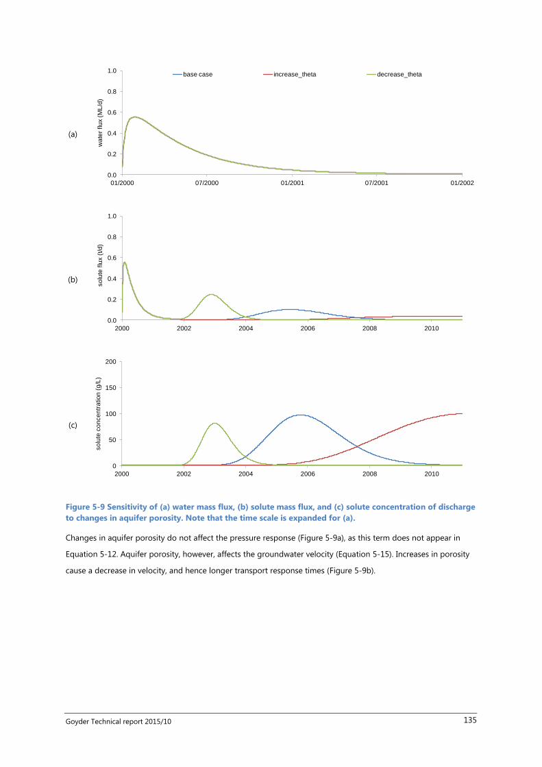
Goyder Technical report 2015/10 135
(a)
(b)
(c)
Figure 5-9 Sensitivity of (a) water mass flux, (b) solute mass flux, and (c) solute concentration of discharge
to changes in aquifer porosity. Note that the time scale is expanded for (a).
Changes in aquifer porosity do not affect the pressure response (Figure 5-9a), as this term does not appear in
Equation 5-12. Aquifer porosity, however, affects the groundwater velocity (Equation 5-15). Increases in porosity
cause a decrease in velocity, and hence longer transport response times (Figure 5-9b).
0.0
0.2
0.4
0.6
0.8
1.0
01/2000 07/2000 01/2001 07/2001 01/2002
wa
ter
flu
x (
ML
/d)
base case increase_theta decrease_theta
0.0
0.2
0.4
0.6
0.8
1.0
2000 2002 2004 2006 2008 2010
so
lute
flu
x (
t/d
)
0
50
100
150
200
2000 2002 2004 2006 2008 2010
so
lute
co
nce
ntr
atio
n (
g/L
)

Goyder Technical report 2015/10 136
(a)
(b)
(c)
Figure 5-10 Sensitivity of (a) water mass flux, (b) solute mass flux, and (c) solute concentration of
groundwater discharge to changes in aquifer specific yield. Note that the time scale is expanded for (a).
Changes in aquifer specific yield affect the pressure response but not the transport response. Aquifer diffusivity is
inversely proportional to specific yield, and so doubling the specific yield produces the same effect as halving
aquifer thickness (compare Figure 5-10 and Figure 5-8).
0.0
0.2
0.4
0.6
0.8
1.0
01/2000 07/2000 01/2001 07/2001 01/2002
wa
ter
flu
x (
ML
/d)
base case increase_Sy decrease_Sy
0.0
0.2
0.4
0.6
0.8
1.0
2000 2002 2004 2006 2008 2010
so
lute
flu
x (
t/d
)
0
50
100
150
200
2000 2002 2004 2006 2008 2010
so
lute
co
nce
ntr
atio
n (
g/L
)

Goyder Technical report 2015/10 137
(a)
(b)
(c)
Figure 5-11 Sensitivity of (a) water mass flux, (b) solute mass flux, and (c) solute concentration of
groundwater discharge to changes in groundwater hydraulic gradient. Note that the time scale is
expanded for (a).
Changes in hydraulic gradient affect the transport response, but not the pressure response (Figure 5-11a and b).
An increase in hydraulic gradient reduces the transport travel time (Figure 5-11b). Doubling hydraulic gradient
has the same effect as halving the porosity (compare Figure 5-11 and Figure 5-9).
Changes in aquifer solute dispersivity affect the transport response, but not the pressure response (Figure 5-12a
and b). Increasing solute dispersivity reduces the salt peak associated with the transport process and reduces the
transport travel time (Figure 5-12b).
0.0
0.2
0.4
0.6
0.8
1.0
01/2000 07/2000 01/2001 07/2001 01/2002
wa
ter
flu
x (
ML
/d)
base case increase_i decrease_i
0.0
0.2
0.4
0.6
0.8
1.0
2000 2002 2004 2006 2008 2010
so
lute
flu
x (
t/d
)
0
50
100
150
200
2000 2002 2004 2006 2008 2010
so
lute
co
nce
ntr
atio
n (
g/L
)

Goyder Technical report 2015/10 138
(a)
(b)
(c)
Figure 5-12 Sensitivity of (a) water mass flux, (b) solute mass flux, and (c) solute concentration of
groundwater discharge to changes in aquifer solute dispersivity. Note that the time scale is expanded for
(a).
5.3.3.3 Potential for negative mass fluxes
The calculation of solute transport by dispersion (Equation 5-15) involves the subtraction of the ambient
groundwater concentration. This raises the possibility for the calculation of negative concentrations and negative
solute fluxes for water discharged to the river. The potential for this problem was examined by assigning an
extremely high specified groundwater concentration (100,000 mg/l) and re-running the model. The solute mass
discharged from groundwater is presented in Figure 5-13.
0.0
0.2
0.4
0.6
0.8
1.0
01/2000 07/2000 01/2001 07/2001 01/2002
wa
ter
flu
x (
ML
/d)
base case increase_Ds decrease_Ds
0.0
0.2
0.4
0.6
0.8
1.0
2000 2002 2004 2006 2008 2010
so
lute
flu
x (
t/d
)
0
50
100
150
200
2000 2002 2004 2006 2008 2010
so
lute
co
nce
ntr
atio
n (
g/L
)

Goyder Technical report 2015/10 139
Figure 5-13 Solute mass (blue) and solute concentration (red) discharged from groundwater for scenario
featuring high specified groundwater concentration.
The high specified groundwater concentration results in the calculation of negative solute mass fluxes. (In fact,
negative values will occur whenever cg > cw.) This may be observed in the reductions in groundwater solute mass
flux and concentration from 2003 to ~2006. These metrics do not return to physically realistic (i.e. nonzero) values
until approximately 5 years have elapsed. Although calculations using Equation (?) do ensure that solute mass
balance will always be preserved, as shown, they do present potential for errors in the calculation of solute mass
fluxes and concentrations in groundwater discharged to a river.
5.3.4 Example 2: Draining wetland model
This example was designed to test the performance of the modified Source software code (a) when realistic
parameter values were specified and (b) when regional groundwater flow was represented.
5.3.4.1 Conceptual model
Compared to the model used previously to identify separate solute breakthrough concentration curves for
groundwater pressure and transport responses, the model used for this example includes some key changes.
First, an additional node and link were added, which enabled the inclusion of an additional specified groundwater
flux at a specified solute concentration. This additional flux represents regional groundwater flow. The
groundwater link parameter values were also changed in order to be more realistic and to be consistent with
values typically used when simulating groundwater–wetland interactions on the lower River Murray. In Source
terminology, this example uses three nodes (i.e. one storage node and two gauge nodes) and two links (i.e. one
groundwater routing-type link [“Groundwater link 1”] and one storage routing-type link [“Groundwater link 2”])
(Figure 5-14). A temporal extent of 51 years (i.e. 2000–2050) was sufficient for model testing purposes.
-10
-8
-6
-4
-2
0
2
-20
0
20
40
60
2000 2002 2004 2006 2008 2010
so
lute
co
nce
ntr
atio
n (
g/L
)
so
lute
flu
x (
t/d
)

Goyder Technical report 2015/10 140
Figure 5-14 Conceptual model used to test the performance of the modified Source software code (a)
when realistic parameter values were specified and (b) when regional groundwater flow was represented.
5.3.4.2 Parameterisation
The wetland (i.e. storage) node served as the up-gradient boundary condition and featured an initial volume
equal to its maximum (and initial) volume of 5,000 ML, distributed over an area of 1 km2. This corresponded to a
maximum stage height of 5 m. The initial concentration of wetland water was specified as 10,000 mg/l and the
bed conductance was specified as 20,000 m2/day. The bed conductance value was manipulated in order to
achieve a maximum linear water flux from the wetland of 0.1 m/day, which is comparable with those measured by
Bramley et al. (2003). An evaporation flux from the wetland was also included, at a rate of 5 mm/day. This value is
consistent with the mean annual evaporation observed at the Loxton Research Centre (http://www.bom.gov.au)
as well as with values observed at Calperum Station (Meyer et al., 2015).
The spatial extent of the wetland was selected arbitrarily, although it is worth noting that fluxes from this area of
floodplain are added to the river at a point. Thus, the calculated fluxes are not associated with any particular
length of river. Rather, different areas of inundation (in terms of square metres of wetland per kilometre of river)
can be simulated either by changing the wetland area or by changing the frequency with which wetlands are
attached to the river.
The groundwater routing link (hereafter “groundwater link 1”) was parameterised as follows. The aquifer
simulated featured hydraulic conductivity = 20 m/day, thickness = 20 m, porosity = 0.3, specific yield = 0.15.
These parameter values are considered representative of the Monoman Formation surficial sand aquifer (Woods
et al., 2014, Woods, 2015a). Other aquifer properties, such as hydraulic gradient = 1 x 10⁻³
, orthogonal distance to
discharge location = 100 m, and solute dispersivity = 1 m, were selected arbitrarily but are considered physically
reasonable. In addition, groundwater was assigned a constant concentration of 10,000 mg/l, which is consistent
with that observed within the floodplain (See Figure 3-25 in Woods (2015a).
For the storage routing-type link located immediately down-gradient of the previously discussed groundwater
link (hereafter “groundwater link 2”), a constant groundwater discharge of 20 m3/day was specified, featuring a
constant concentration of 10,000 mg/l.
All parameter values specified for the model are summarised in Table 5-3.
.
Table 5-3 Model parameter values

Goyder Technical report 2015/10 141
Model element Parameter Value Units
Wetland storage node bed conductance 20,000 m2/day
wetland area 106 m
2
initial water volume 5,000 ML
initial solute concentration 10,000 mg/l
Groundwater storage link aquifer hydraulic conductivity 20 m/day
aquifer thickness 20 m
aquifer porosity 30 %
aquifer specific yield 0.15 -
groundwater hydraulic gradient 1 x 10⁻³
-
orthogonal distance to discharge location 100 m
solute dispersivity 1 m
solute concentration 10,000 mg/l
5.3.4.3 Results
Modelling results are presented in terms of water mass fluxes, solute mass fluxes, and solute concentrations
(Figure 5-15). It should first be noted that, due to the parameter values specified in this test case, separate
pressure and transport responses cannot be distinguished from one another; instead, both responses occur on
similar timescales. The rate of water infiltration though the base of the wetland to groundwater commences at
100 ML/day and declines exponentially to zero after approximately one year elapsed. The rates of discharge from
groundwater links 1 and 2 (which are almost identical) commence at ~10 ML/day. As the propagation of hydraulic
pressure resulting from wetland discharge reaches the far extent of the aquifer, the rate of groundwater discharge
rises to ~55 ML/day at ~3 months elapsed. The rate of groundwater discharge declines exponentially thereafter.
Note that the time series of discharge rate from groundwater link 2 is almost identical to that of groundwater link
1. This is because the specified additional influx due to regional groundwater flow was insignificant (0.02 ML/day)
in comparison to that resulting from wetland infiltration.

Goyder Technical report 2015/10 142
(a)
(b)
(c)
Figure 5-15 (a) Water mass fluxes, (b) solute mass fluxes and (c) solute concentrations of water exiting the
wetland (blue), groundwater link (red) and groundwater link 2 (green). Note that the time scale is
compressed for (c).
The rate of solute mass infiltrated though the base of the wetland to groundwater commences at 1,000
tonnes/day and declines exponentially to zero after ~1 years elapsed. The rates of solute mass flux from both
groundwater links commence at ~200 tonnes/day. The solute mass transported can be observed in the peak rate
of ~550 tonnes/day occurring after less than three months elapsed. This response, which combined both pressure
and transport responses, persists until ~1 year has elapsed.
The solute concentration of water exiting the wetland increased from ~10,000 mg/l to ~25,000 mg/l at ~2.5 years
elapsed, at which time infiltration from the wetland ceases. This increase in wetland solute concentration is due to
evapotranspiration. The solute concentration of discharge from groundwater link 1 increases from 10,000 mg/l to
a maximum of ~35,000 mg/l after ~4 years elapsed. Similarly, the solute concentration of discharge from
0
20
40
60
80
100
01/2000 04/2000 07/2000 10/2000 01/2001
wa
ter
flu
x (
ML
/d)
floodplain discharge groundwater link 1 groundwater link 2
0
200
400
600
800
1000
01/2000 04/2000 07/2000 10/2000 01/2001
so
lute
flu
x (
t/d
)
0
10
20
30
40
50
2000 2002 2004 2006 2008 2010 2012 2014 2016 2018 2020
so
lute
co
nce
ntr
atio
n (
g/L
)

Goyder Technical report 2015/10 143
groundwater link 2 increases from 10,000 mg/l to a maximum of ~25,000 mg/l after ~4 years elapsed. As
discussed above, these high concentrations result from slight differences in the temporal patterns of the pressure
and transport responses to infiltration. This means that water and salt fluxes can occur at different times, resulting
in anomalous concentrations when salt flux is divided by water flux. However, these anomalies are unlikely to be
observed when river concentrations (rather than groundwater discharge concentrations) are considered.
5.3.4.4 Sensitivity analyses
In order to test the sensitivity of the representations of groundwater flow and solute transport to parameter
variation, the one-at-a-time approach was again undertaken (Figure 5-16 – Figure 5-21). For the parameter values
examined, changes in aquifer hydraulic conductivity appear to be nonlinearly related to peak water and solute
fluxes and the arrival times thereof (Figure 5-16a and b). For example, in comparison to the base case scenario,
increases and decreases in hydraulic conductivity result in reductions in both peak water and solute mass fluxes.
Peak solute concentration is positively correlated with aquifer hydraulic conductivity, while the timing of this
response is inversely correlated (Figure 5-16c).

Goyder Technical report 2015/10 144
(a)
(b)
(c)
Figure 5-16 Sensitivity of (a) water mass flux, (b) solute mass flux, and (c) solute concentration of
groundwater discharge to changes in aquifer hydraulic conductivity. Note that the time scale is
compressed for (c).
0
10
20
30
40
50
60
01/2000 04/2000 07/2000 10/2000 01/2001
wa
ter
flu
x (
ML
/d)
base case increase_K decrease_K
0
100
200
300
400
500
600
01/2000 04/2000 07/2000 10/2000 01/2001
so
lute
flu
x (
t/d
)
10
20
30
40
50
2000 2005 2010 2015 2020 2025 2030
so
lute
co
nce
ntr
atio
n (
g/L
)

Goyder Technical report 2015/10 145
(a)
(b)
(c)
Figure 5-17 Sensitivity of (a) water mass flux, (b) solute mass flux, and (c) solute concentration of
groundwater discharge to changes in aquifer thickness. Note that the time scale is compressed for (c).
For the parameter values examined, changes in aquifer thickness appear to be nonlinearly related to peak water
and solute fluxes and the arrival times thereof (Figure 5-17a and b). For example, in comparison to the base case
scenario, increases and decreases in aquifer thickness result in reductions in both peak water and solute fluxes.
Peak solute concentration is positively correlated with aquifer thickness, while the timing of this response is
insensitive to variations in aquifer thickness (Figure 5-17c).
0
10
20
30
40
50
60
01/2000 04/2000 07/2000 10/2000 01/2001
wa
ter
flu
x (
ML
/d)
base case increase_b decrease_b
0
100
200
300
400
500
600
01/2000 04/2000 07/2000 10/2000 01/2001
so
lute
flu
x (
t/d
)
10
20
30
40
50
2000 2005 2010 2015 2020 2025 2030
so
lute
co
nce
ntr
atio
n (
g/L
)

Goyder Technical report 2015/10 146
(a)
(b)
(c)
Figure 5-18 Sensitivity of (a) water mass flux, (b) solute mass flux, and (c) solute concentration of
discharge to changes in aquifer porosity. Note that the time scale is compressed for (c).
Changes in aquifer porosity have minimal effect on both water and solute fluxes and the timing of these
responses (Figure 5-18a and b). Peak solute concentration is inversely correlated with porosity, while the timing of
this response is positively correlated (Figure 5-18c).
0
10
20
30
40
50
60
01/2000 04/2000 07/2000 10/2000 01/2001
wa
ter
flu
x (
ML
/d)
base case increase_theta decrease_theta
0
100
200
300
400
500
600
01/2000 04/2000 07/2000 10/2000 01/2001
so
lute
flu
x (
t/d
)
10
20
30
40
50
2000 2005 2010 2015 2020 2025 2030
so
lute
co
nce
ntr
atio
n (
g/L
)

Goyder Technical report 2015/10 147
(a)
(b)
(c)
Figure 5-19 Sensitivity of (a) water mass flux, (b) solute mass flux, and (c) solute concentration of
groundwater discharge to changes in aquifer specific yield. Note that the time scale is compressed for (c).
For the parameter values examined, changes in aquifer specific yield appear to be nonlinearly related to peak
water and solute fluxes and the arrival times thereof (Figure 5-19a and b). For example, in comparison to the base
case scenario, increases and decreases in specific yield result in reductions in both peak water and solute fluxes.
Peak solute concentration is inversely correlated with specific yield, while the timing of this response appears
insensitive to variations in specific yield (Figure 5-19c).
0
10
20
30
40
50
60
01/2000 04/2000 07/2000 10/2000 01/2001
wa
ter
flu
x (
ML
/d)
base case increase_Sy decrease_Sy
0
100
200
300
400
500
600
01/2000 04/2000 07/2000 10/2000 01/2001
so
lute
flu
x (
t/d
)
10
20
30
40
50
2000 2005 2010 2015 2020 2025 2030
so
lute
co
nce
ntr
atio
n (
g/L
)

Goyder Technical report 2015/10 148
(a)
(b)
(c)
Figure 5-20 Sensitivity of (a) water mass flux, (b) solute mass flux, and (c) solute concentration of
groundwater discharge to changes in groundwater hydraulic gradient. Note that the time scale is
compressed for (c).
Changes in groundwater hydraulic gradient have minimal effect on both water and solute fluxes and the timing of
these responses (Figure 5-20a and b). An increase in peak solute concentration and a reduction in the time
required to reach peak concentration are observed when the hydraulic gradient is increased. Conversely, inverse
trends are observed when the hydraulic gradient is decreased (Figure 5-20c).
0
10
20
30
40
50
60
01/2000 04/2000 07/2000 10/2000 01/2001
wa
ter
flu
x (
ML
/d)
base case increase_i decrease_i
0
100
200
300
400
500
600
01/2000 04/2000 07/2000 10/2000 01/2001
so
lute
flu
x (
t/d
)
10
20
30
40
50
2000 2005 2010 2015 2020 2025 2030
so
lute
co
nce
ntr
atio
n (
g/L
)

Goyder Technical report 2015/10 149
(a)
(b)
(c)
Figure 5-21 Sensitivity of (a) water mass flux, (b) solute mass flux, and (c) solute concentration of
groundwater discharge to changes in aquifer solute dispersivity. Note that the time scale is compressed
for (c).
Changes in aquifer solute dispersivity have minimal effect on both water and solute fluxes and the timing of these
responses (Figure 5-21a and b). Peak solute concentration is inversely correlated with solute dispersivity.
In summary, both water and solute fluxes appear to be insensitive to variations in aquifer porosity, solute
dispersivity and hydraulic gradient. The sensitivity of water and solute fluxes to variations in all other parameters
tested was also very limited. Peak solute concentration was positively correlated with aquifer hydraulic
conductivity and thickness and inversely correlated with porosity, specific yield and solute dispersivity. The timing
of peak solute concentration was inversely correlated with aquifer hydraulic conductivity, positively correlated
with aquifer porosity, and relatively insensitive to all other parameter variation.
0
10
20
30
40
50
60
01/2000 04/2000 07/2000 10/2000 01/2001
wa
ter
flu
x (
ML
/d)
base case increase_Ds decrease_Ds
0
100
200
300
400
500
600
01/2000 04/2000 07/2000 10/2000 01/2001
so
lute
flu
x (
t/d
)
10
20
30
40
50
2000 2005 2010 2015 2020 2025 2030
so
lute
co
nce
ntr
atio
n (
g/L
)

Goyder Technical report 2015/10 150
5.3.5 Example 3: Coupled river model
This example aimed to test the operation of the groundwater flowpath in a model that includes surface flows
between the river and the wetland. The wetland was initially filled with a small volume of highly saline water to
allow the model to develop a residual salt mass in the wetland. After a period of time, overbank flow from the
river to the wetland during a high flow event inundates the wetland and subsequently some of this water
infiltrates the soil and reaches the groundwater. The infiltrated water and solute were then conveyed back to a
downstream section of river via groundwater. The model serves as an example of how the modifications to
SOURCE groundwater functionality may be used to represent river–wetland–groundwater interactions.
5.3.5.1 Conceptual model
The model simulates the movement of water and solute from a river to a wetland via a surface channel, then back
to the river via groundwater (Figure 5-22). In Source terminology, this was represented using five nodes (i.e. one
inflow node, one wetland hydraulic connector node, one storage node, one gauge node, and one confluence
node) and numerous links of various types. A temporal extent of 21 years (i.e. 2000-2021) was sufficient for model
testing purposes.
Figure 5-22 Conceptual model used to represent river–wetland–groundwater interactions for testing of
the modified version of Source
The river inflow node served as the up-gradient boundary condition and featured a constant flow of 5,000
ML/day except for a three month-long period (June to August) of the second year, during which the inflow
increased gradually to a maximum rate of 5,200 ML/day and subsequently declined to return to a rate of 5,000
ML/day. This variation in flow rate was calculated according to a sine function, defined arbitrarily as:
(5-15)
After this period, river inflows were kept at 5,000 ML/day for the remainder of the 21 year simulation. In practice,
a peak flow of 5,200 ML/day on the lower River Murray would not normally be sufficient to instigate overbank

Goyder Technical report 2015/10 151
flow and wetland inundation. However, for the purposes of the present modelling, this increase in flow serves to
initiate flow to, and inundation of, a wetland storage node.
Flow from the river node was directed to a wetland hydraulic connector (WHC) node, which represented the
diversion of water to a wetland located adjacent to the river. The volume of diversion was calculated according to
the hydraulic gradient between the wetland and the river. Inflows to the WHC node were related to river stage
heights through a specified flow versus stage relationship. Essentially, while river flow remained less than 5,200
ML/day, no water was diverted to the wetland. Upon the onset of peak flows, the elevation of water at the WHC
node was increased linearly from zero to a maximum of 5 m for a peak flow rate of 5,200 ML/day. The rate at
which water was conveyed to the wetland was calculated according to a specified stage versus conveyance flux
relationship. For a surface water channel elevation of 5 m, the equivalent rate of water conveyed was specified as
2 m2.5
/s.
The conveyance link was specified as a bidirectional link. This enabled flows to return to the WHC node from the
wetland storage node after the reversal of the hydraulic gradient, which occurred after 24 days of increased river
flows.
The return of infiltrated wetland water to the river via groundwater at a location downstream of the WHC node
was represented by a confluence node.
5.3.5.2 Parameterisation
The wetland storage node featured an initial volume of 1 ML distributed over an area of 1 km2. This corresponded
to an initial stage height of 1 x 10⁻³
m. The initial concentration of wetland water was specified as 100,000 mg/l.
This combination of limited initial stage height and hypersaline initial concentration represents a nearly dry
floodplain in which the evapo-concentration of salt has occurred. Wetland bed conductance was specified as
2000 m2/day. An evaporation flux from the wetland was also included, at a rate of 5 mm/day.
3
The groundwater routing link (hereafter “groundwater link 1”) was parameterised as in Table 5-4. This link
represents flows between the wetland and the river. A constant groundwater concentration is used in the
pressure equation, and this example used a value of 100,000 mg/l.
For the storage routing-type link located immediately down-gradient of the previously discussed groundwater
link (hereafter “groundwater link 2”), a constant groundwater discharge of 0.1 m3/day was specified, also with a
constant concentration of 100,000 mg/l. Groundwater link 2 represents regional groundwater flow to the river.
All other parameter values and initial conditions specified for the model are summarised in Table 5-4.
3 The evaporation routine in Source specifies a depth-area relationship, which allows the floodplain to reduce in
area as the floodplain shrinks. The total evaporation from the floodplain is therefore not constant, but rather is a
function of water depth.

Goyder Technical report 2015/10 152
Table 5-4 Model parameter values.
Model element Parameter Value Units
River inflow node Initial flow rate 5,000 ML/day
Peak flow rate 5,200 ML/day
Solute concentration 500 mg/l
WHC* node maximum average flow 5,200 ML/day
maximum elevation 5 m
Conveyance link maximum modified conveyance 2 m2.5
.s-1
maximum elevation 5 m
Wetland storage node wetland area 106 m
3
initial storage volume 1 ML
bed conductance 2,000 m2/day
initial solute concentration 100,000 mg/l
Groundwater link 1 aquifer hydraulic conductivity 1 m/day
aquifer thickness 20 m
aquifer porosity 10 %
aquifer specific yield 0.15 -
hydraulic gradient 1 x 10⁻³
-
orthogonal distance to discharge location 1,000 m
solute dispersivity 1 m
solute concentration 100,000 mg/l
Groundwater link 2 water flux 0.1 m3/day
solute concentration 100,000 mg/l
*wetlands hydraulic connector

Goyder Technical report 2015/10 153
5.3.5.3 Results
Modelling results are presented in terms of water mass fluxes, solute mass fluxes, and solute concentrations.
Water mass fluxes reported by the model for the first two years are first presented (Figure 5-23).
Model inflow at the river inflow node (Figure 5-23a) remains constant at 5,000 ML/day until 01/06/2001, at which
time it increases gradually to a maximum rate of 5,200 ML/day (on 15/8/2001) before returning to the initial rate
of 5,000 ML/day at 01/09/2001. The diversion of water to the wetland storage node (Figure 5-23b) commences at
01/06/2001 and increases to a maximum rate of 170 ML/day at 07/07/2001.
(a)
(b)
(c)
Figure 5-23 Fluxes of water (a) entering the model at the river inflow node, (b) diverted to the wetland
storage node via the wetlands hydraulic connector (WHC) node, and (c) flowing downstream from the
WHC node.
4950
5000
5050
5100
5150
5200
5250
01/2001 04/2001 07/2001 10/2001 01/2002 04/2002 07/2002 10/2002 01/2003
wa
ter
flu
x (
ML
/d)
river inflow
-100
-50
0
50
100
150
200
01/2001 04/2001 07/2001 10/2001 01/2002 04/2002 07/2002 10/2002 01/2003
wa
ter
flu
x (
ML
/d)
diverted flow
4950
5000
5050
5100
5150
5200
5250
01/2001 04/2001 07/2001 10/2001 01/2002 04/2002 07/2002 10/2002 01/2003
wa
ter
flu
x (
ML
/d)
non-diverted flow

Goyder Technical report 2015/10 154
River flow is diverted to the wetland storage node until 25/07/2001, at which time the hydraulic gradient reverses
and water flows back from the wetland to the river. A maximum return flow rate of 81 ML/day occurs on
17/08/2001 and surface return flow persists until 03/08/2001.
Non-diverted flow (Figure 5-23c) increases initially as river inflows increase, then decreases as diverted flows
increase. Non-diverted flow subsequently increases, reaching a maximum rate of more than 5,200 ML/day. The
additional flow (in excess of river inflow) is derived from return flow from the wetland storage node. Non-diverted
flow subsequently decreases, commensurate with the reduction in river inflows.
(a)
(b)
(c)
Figure 5-24 (a) Water mass fluxes, (b) solute mass fluxes and (c) solute concentrations of water exiting the
wetland (blue) and the groundwater domain (red). Note that the time scale is compressed for (c).
Wetland discharge commences at 2 x 10⁻³
ML/day and gradually declines to ~4 x 10⁻⁴
ML/day on 02/06/2001,
although this is not apparent on the scale used for Figure 5-24a. This represents the infiltration of the initial water
4850
4950
5050
5150
5250
0
2
4
6
8
10
01/2001 04/2001 07/2001 10/2001 01/2002 04/2002 07/2002 10/2002 01/2003
wa
ter
flu
x (
ML
/d)
floodplain discharge river confluence
2450
2500
2550
2600
2650
2700
2750
-10
0
10
20
30
40
50
01/2001 04/2001 07/2001 10/2001 01/2002 04/2002 07/2002 10/2002 01/2003
so
lute
flu
x (
T/d
)
floodplain discharge river confluence
499
500
501
502
503
504
-50000
0
50000
100000
150000
200000
2000 2002 2004 2006 2008 2010 2012 2014 2016 2018 2020
so
lute
co
nce
ntr
atio
n (
mg
/L)
floodplain discharge river confluence

Goyder Technical report 2015/10 155
volume stored on the wetland. Wetland discharge subsequently increases to a maximum rate of ~9.9 ML/day on
31/09/2001 before declining exponentially to zero over the 16 month-long period following peak river flow. Flow
at the river confluence node is almost identical to that observed downstream of the WHC node, which indicates
the insignificant contribution of wetland–groundwater discharge to river flow.
The solute mass flux of wetland discharge commences at ~0.2 tonnes/day and gradually declines to ~0.07
tonnes/day prior to the arrival of diverted river flows (Figure 5-24b). The solute mass flux subsequently increases
to a maximum rate of ~46 tonnes/day on 31/09/2001 before declining exponentially on 12/09/2007. Solute mass
flux dynamics at the river confluence node reflect those of river confluence water fluxes, increasing from 2,500
tonnes/day on 25/07/2001 before declining to ~2,502 tonnes/day by the end of the 21 year-long simulation.
The solute concentration of water exiting the wetland commences at 100,000 mg/l, which is consistent with the
specified initial condition (Figure 5-24c). Due to the effect of evapoconcentration, wetland discharge
concentrations increase to ~168,000 mg/l at 02/06/2001. The concentration then drops to 500 mg/l during the
flooding event. As the wetland dries out, evaporation causes the wetland discharge concentrations to increase to
~83,000 mg/l at 29/06/2015.
In addition to the water flux, solute mass flux and solute concentration of water discharged from the wetland
storage node, the mass of solute stored in the wetland was also reported (Figure 5-25). The initial stored mass of
~100 tonnes decreases to ~34 tonnes prior to the arrival of diverted river flows. The stored solute mass then
increased to a maximum of ~2,500 tonnes on 24/07/2001 before declining exponentially to zero on 17/07/15.
Because Source models leakage as proportional to the water depth, leakage decreases to zero as the water depth
decreases to zero. This causes the wetland to drain much more slowly than would usually be the case.
Figure 5-25 Wetland salt mass storage
In this example, a very shallow initial wetland water depth (1 mm) with high concentration (100,000 mg/l) was
implemented to create an initial salt mass. Because the evaporation rate (5 mm/day) is much greater than the
leakage rate at this water depth, it was expected that the water would evaporate leaving remnant salt that would
be mobilised by the next flooding event. However, this did not eventuate because evaporation decreases with
water depth. (The evaporation routine in Source essentially assumes that the reduction in water volume
represents a reduction in wetland area rather than water depth.) However, as currently implemented, the leakage
routine does not operate in this same manner. This means that the wetland inevitably dries out by leakage rather
than by evaporation, which means that no salt mass is retained in the wetland. The final output of a zero stored
0
500
1000
1500
2000
2500
3000
01/2001 04/2001 07/2001 10/2001 01/2002 04/2002 07/2002 10/2002 01/2003
sto
red
ma
ss (
T)

Goyder Technical report 2015/10 156
salt mass in this example raises questions about the ability of the current routines in Source to accurately account
for the mass of dry salt stored in the surface sediments of a wetland and/or in sediments of the unsaturated zone
beneath a wetland.
5.3.6 Summary
The approach for simulating groundwater flow from the wetland to the river functioned efficiently when coded
into Source. Sensitivity analysis showed that changes in salt load responded to changes in aquifer parameters as
expected from the governing equations. It is important to note, however, that the salt loads calculated from the
model represent fluxes from a small area of floodplain (1 km2) for single inundation events. Although model
parameters are within the range of values measured on the floodplain (Woods, 2015a), converting model fluxes
to mean fluxes per kilometre of river requires consideration of area and frequency of inundation (per kilometre
length of river). This was beyond the scope of the present study, but it is an important next step. However, there
are a number of areas where model improvements could be made, and these improvements should precede any
comparison with field data. In particular:
The routines do have the potential to produce negative salt fluxes to the river. This was demonstrated in
a model simulation where parameters were deliberately chosen to separate the pressure and transport
processes. The problem did not arise in a subsequent model simulation using more realistic model
parameters, chosen to be representative of the lower River Murray and its wetlands. However, it is not
yet clear how often this problem will arise.
The current model appears unable to retain salt mass in the wetland if it dries out between flood events.
It appears that this occurs because the evaporation routine specifies a bathymetric function to reduce
evaporation as wetland volume decreases (simulating a reduction in wetland area). However, this
bathymetry function is not currently used by the leakage routine. This model inconsistency should be
relatively straightforward to fix. However, it currently means that the wetland tends to dry by leakage
rather than by evaporation, and so all of the salt is removed with the leakage.
The model assumes that leakage is proportional to water depth. In reality, however, gravity drainage
should still occur when the water depth is zero. By not including this process, the wetland dries more
slowly than should be the case. Whether this discrepancy is significant for modelling salt fluxes to the
river has yet to be determined.
5.4 Floodplain Groundwater Velocity and Travel Times
5.4.1 Outline
One of the critical parameters used by the above model is the regional groundwater velocity (which is calculated
from the regional groundwater gradient, the aquifer hydraulic conductivity and the porosity). The model assumes
that this velocity is constant, whereas in reality it is likely to change over time due to infiltration events on the
floodplain. Here, we compare the timing of salt loads to the river calculated using a constant velocity with those
calculated by a model that allows the groundwater velocity to be calculated from the wetland leakage. The
approach is directly analogous to flow in a pipe, with the wetland forming one end of the pipe, and discharge to
the river at the other end. Water only moves through the pipe when the wetland is leaking. (At other times the
velocity is zero.) Because the volume of the pipe is fixed, when water enters the upstream end of the pipe through
the base of the wetland, water immediately moves out the other end of the pipe into the river. This represents the
pressure effect. Of course, the model represents the pressure effect as instantaneous, whereas in reality it would
be somewhat delayed. A third model includes vegetation extraction along the flow path. The mechanics of the
three models is described below.

Goyder Technical report 2015/10 157
5.4.2 Formulation
5.4.2.1 Surface Water Module
The main input data for all the models are river stage heights over time. Flow between the river and wetland is
then controlled by a sill height. When water level in the river (or wetland ) exceeds the sill height, then flow
between the two water bodies is calculated using the Manning Equation. (Water flows from the river to the
wetland , when the river stage exceeds the sill height and exceeds the water level in the wetland . Water flows
back from the wetland to the river when the water level in the wetland exceeds the sill height and exceeds the
river stage.) The wetland area is constant, so that changes in the water depth in the wetland are given by
(5-16)
where h is the wetland water depth, Qin is surface flow from the river to the wetland , Qout is surface flow from the
wetland to the river, E is the evaporation rate from the wetland , q is the wetland leakage rate, A is wetland area
and t is time. The river stage is prescribed in the model input file and does not change due to water flow to the
wetland. Similarly, changes in the wetland salt store are given by:
(5-17)
where M is the salt mass in the wetland , c is the solute concentration in the wetland , criv is the concentration in
the river (which is assumed to be constant in time). The salt concentration in the wetland is simply calculated as
the mass divided by the water depth (c=M/h), except that it is constrained by a maximum concentration
(equivalent to the saturation point). Thus when M/h exceeds the saturation point, the salt is assumed to be only
partly dissolved, and partly as precipitated crystals. The model restricts the fluxes to the dissolved part.
The leakage rate beneath the wetland is assumed to be proportional to the water depth, and is given by:
(5-18)
where h is the depth of water in the wetland, hc is the thickness of a low permeability layer at the base of the
wetland, and Kc is the saturated hydraulic conductivity of this layer.4
5.4.2.2 Groundwater Module
Three different models were constructed, all based on slightly different process conceptualisations. The different
conceptualisations lead to different travel times for salt between the wetland and the river. In each case, the salt
mass flux to the river is calculated as
(5-19)
where ts is the salt travel time between the wetland and the river, and CL is the salt concentration of wetland
leakage, and t is time. Note, however, that the travel time is not necessarily a constant value, but can change over
time. The left hand side of Equation 5-19 is the salt flux to the river per unit length of river that parallels the
wetland.
The three models are summarised as:
4 This formulation is slightly different to that used by the Source model. (Compare Equations 5-11 and 5-18.) The
Source model assumes that leakage is proportional to water depth, whereas the Fortran model assumes that
leakage is proportional to (h+hc). The latter approach is more correct, because if the floodplain soil is saturated,
then the floodplain will still drain even though there may be no surface water (Brunner et al., 2009).

Goyder Technical report 2015/10 158
1. Constant velocity model. This model moves infiltration back to the river at a constant velocity, which is
specified. This is the approach used for the transport component of the SOURCE model. The travel time
(ts) of salt between the wetland and the river is therefore given by
(5-20)
where x is the distance between the river and the wetland (see Figure 5-4) and v is the velocity. The salt
flux to the river is then simply calculated using Equation 5-19. The model does not allow the leakage of
water beneath the wetland to affect this velocity. The model is therefore perhaps most appropriate for a
system with a large regional groundwater gradient, where the mean leakage rate beneath the wetland is
small relative to the regional flow rate. This approach does not include a pressure effect, but this may be
unimportant if there is a strong regional hydraulic gradient and the volumes of recharge are small. Of
course, the problem with implementing this model is that the groundwater velocity must be known.
2. Pipe model. This model allows the velocity of water to change in time, based on changes in the wetland
leakage rate. Each parcel of infiltration is essentially pushed by subsequent infiltration. When the
wetland is dry and there is no infiltration, the groundwater velocity is zero. The water velocity is a
function of the infiltration rate beneath the wetland, given by:
(5-21)
where w is the width of the wetland and b is the aquifer thickness (Figure 5-26). The travel time (t’)
between infiltration and discharge for a particle leaking beneath the wetland at time t0 can be calculated
from:
(5-22)
where x is the distance between the wetland and the river and v(t) is the water velocity along the
flowpath.
Figure 5-26 Schematic representation of groundwater flow from a wetland to a river. The wetland leakage
flux is qw, and the flux to the river is vb. Both quantities have units of L2/T, and represent fluxes per
metre length of river.

Goyder Technical report 2015/10 159
3. Pipe Model with Vegetation Extraction. This model moves water towards the river as the single pipe
model, but also allows water to be extracted by vegetation along the flowpath. This reduces the
groundwater velocity. This process also concentrates salt, however the total salt flux does not change –
the discharge is just delayed. The travel time (t’) between infiltration and discharge for a particle leaking
beneath the wetland at time t0 can be calculated as:
(5-23)
where Et is the evapotranspiration rate along the flowpath. (The model actually uses a slightly different
approach, in which x is replaced by x-w/2 if the wetland contains water and x+w/2 if the wetland is dry.
This allows for evapotranspiration to also occur beneath a dry wetland.)
5.4.3 Example
The model was run using historic water level data from Lock 5 as the input. Data from 1 January 1936 till 1 July
2013 was used, during which time the river level varied between 12.55 and 19.46 m. The data was duplicated to
form a sequence of 155 years of daily river stage data for the simulations. Duplication of the data was necessary
because of the long travel times along the groundwater flowpath between the wetland and the river. Other model
parameters are given in
Table 5-5.
Table 5-5 List of groundwater parameters for different models
Symbol Description Value Units
A Area of wetland 100,000 m2
b Aquifer thickness 100 m
criv Concentration in river 500 mg/L
cmax Maximum permissible concentration 200,000 mg/L
E Wetland evaporation rate 0.005 m/day
1Et Evapotranspiration rate 0.001 m/day
hc Thickness of wetland bed 1 m
Kc Hydraulic conductivity of wetland bed 0.02 m/day
2v Groundwater velocity 0.05 m/day
w Width of wetland 100 m
x Distance of wetland from the river 250 m
Aquifer porosity 0.4 -
1 Vegetation model only
2 Constant velocity model only

Goyder Technical report 2015/10 160
Figure 5-27 shows the river level, wetland level, flow rate between the river and wetland and leakage rate beneath
the wetland over half of the simulation period. For these simulations the base of the river was assumed to be at
15 m, and the sill height was 16 m. As can be seen flows from the river to the wetland commences only when the
river level exceeds the sill height of 16 m. Return flow from the wetland to the river (shown as negative flows on
Figure 5-27c) occur when the river level drops below the sill height. Leakage beneath the wetland occurs
whenever the wetland contains water (level above 15 m in this simulation). The leakage rate is proportional to the
depth of water in the wetland.
Figure 5-27 River and wetland levels, flow rate between the river and the wetland and leakage rate
beneath the wetland for a sill height of 16 m. The leakage rates form the input flux for the groundwater
flow module in each of the different models.
The surface water fluxes and leakage rate are the same for all three models. Figure 5-28 and Figure 5-29 show
wetland leakage salt flux (also the same for all three models) and the salt flux to the river for the three different
models. (Figure 5-28 uses a logarithmic scale for salt flux, whereas Figure 5-29 uses a linear scale.) Note that
wetland leakage salt flux for each event is initially high, and then drops, but increases again as the wetland dries
out. This is shown more clearly in Figure 5-30, which highlights the salt leakage from the flood event between
5600 and 5850 days. The initial high rate of salt infiltration is due to salt which was stored within the wetland prior
to the flood event. As flood waters enter the wetland, they bring in relatively fresh water, and so the salt flux
decreases (even though the rate of water leakage may increase). (The water leakage rate peaks at approximately
5650 days in this case.) After 5780 days, both the river and wetland have dropped below the sill height. The
subsequent increase in flux is due to the increase in salinity in the wetland due to evaporation.
The maximum salt flux in wetland leakage over the simulation period is approximately 427 tonnes/day/km, and
these high fluxes tend to occur when the concentration is high and the leakage rate is relatively low. For the
constant velocity model, a constant velocity of 0.05 m/day was specified. The salt flux to the river is therefore
simply equal to the salt leakage flux, delayed by a travel time of 5,000 days. (The wetland distance is 250 m, and

Goyder Technical report 2015/10 161
hence 250 m / 0.05 m/day = 5,000 days.) For the single pipe model, the maximum salt flux to the river is 2,140
tonnes/day/km. The higher salt flux occurs because groundwater velocity is high during leakage events, and so
more saline water is displaced to the river. For the vegetation model, the saline groundwater becomes
concentrated by evapotranspiration, and so this effect is more pronounced, with a maximum salt flux to the river
of 26,600 tonnes/day/km.
For the pipe model, each wetland leakage event is accompanied by a salt discharge to the river. This is the
pressure effect of leakage, which is instantaneous in this model. In fact, the water leakage rate will be equal to the
water flux to the river. However, the salt flux to the river is different to the salt flux in leakage, because the water
may have a different concentration.
Figure 5-28 Salt flux leaking beneath the wetland, and salt flux to the river under three different

Goyder Technical report 2015/10 162
groundwater flowpath conceptualisations. Note that y-axis scales are logarithmic.
Figure 5-29 Salt flux leaking beneath the wetland , and salt flux to the river under three different
groundwater flowpath conceptualisations. This figure contains the same data as Figure 26, except that salt
flux is shown using a linear scale. Because of this, some of the smaller salt fluxes are not visible on this
figure.
Figure 5-30 Water and salt flux beneath the wetland for a single filling and draining event
Figure 5-31 indicates travel times to the river for salt infiltrating in two particular events: one centred around Day
5,070 and a second centred on Day 8,400. As discussed above, travel times for the constant velocity model are
5,000 days in each case, and so this salt arrives at the river in Days 10,070 and 13,400 respectively. For the pipe
model, travel times are much longer. This is because there is no flow towards the river when the wetland is dry.
The travel time for the first event is 13,230 days, and hence it reaches the river on Day 18,300. The travel time for
the second event is 23,630 days, and so it reaches the river on Day 32,030. The first event travels more quickly to
the river, because it is followed by a number of other infiltration events, which push it. In contrast the second
even occurs before a dry period, and so it moves more slowly. The vegetation model has even longer travel times
because extraction of water by the vegetation slows down the water velocity.

Goyder Technical report 2015/10 163
Figure 5-31 Salt flux leaking beneath the wetland, and salt flux to the river under four different groundwater flowpath conceptualisations. The travel time of leakage
is shown for each of the models, for two particular leakage events. Salt flux to the river is not shown for the first 25,000 days, due to model warm-up (i.e.
equilibration of initial conditions).

Goyder Technical report 2015/10 164
5.4.4 Summary
Three different methods of calculating groundwater velocity between a wetland and river were compared. The first
conceptualisation used a constant velocity and resulted in salt fluxes to the river that were unrelated to river flow rates. The
second approach, whereby the groundwater velocity was related to the wetland leakage rate, resulted in salt fluxes to the river
that only occur at times of wetland leakage. This model produced larger peak salt loads to the river than are produced by the
constant velocity model. The model with vegetation extraction of groundwater has the largest peak salt loads and longest
groundwater travel times.
The use of a constant velocity for the movement of salt between the wetland and river is likely to be realistic if the regional
groundwater velocity is high relative to the wetland leakage rate. However, whether this condition is met across all of the River
Murray floodplain areas is unclear. The comparison in this section, shows that salt fluxes and travel times are highly dependent
upon the method used to determine the groundwater velocity. Further analysis of how groundwater velocity changes with time
within river floodplain environments would therefore assist our understanding of salt transport between wetlands and the river.
5.5 Discussion and conclusions
The Source model (Welsh et al., 2012) has been widely promoted as a tool for simulating river flows and dissolved salt
concentrations. The model also includes some limited groundwater functionality, with the capacity to simulate changes in
groundwater flow to the river due to irrigation leakage or groundwater pumping. The current project has developed a simple
approach for including salt transport on river floodplains. Surface water exchange between the river and inundated areas of the
floodplain are simulated using existing surface water routines within the model. The new routines allow flow of water and salt
back to the river through groundwater pathways.
There are two important components to this salt movement. The first is related to the pressure response created by the
groundwater mound caused by leakage of floodwaters into the regional aquifer. The salt flux induced by this pressure
response is unrelated to the salinity of the leakage water. The second component is the transport of the leakage water back to
the river. This transport occurs more slowly, but the salt flux is determined by the concentration of the leakage water. An
approach for simulating both the pressure and transport processes between a wetland and the river was developed and
incorporated into a version of the Source model. The model represents areas of floodplain inundation using wetlands. These
wetlands fill from overbank flows from the river, and dry by surface water return flows, evaporation and leakage. Although each
wetland is represented using simple, average parameter values (e.g., wetland bed thickness and hydraulic conductivity), more
complex patterns of inundation could be represented using multiple wetlands.
A number of simple simulations were performed using the model to test that the model equations were coded correctly and
that the calculated water and salt fluxes to the river were consistent with the conceptual model. However, due to time
constraints within the project, only a relatively small number parameter values were used, and hence further testing is
desirable. Based on the testing carried out to date, a number of observations and areas where the model could be further
improved were noted:
1. The approach has the potential to calculate negative groundwater discharge concentrations under certain conditions.
This was not encountered during the initial simulations, but was demonstrated in a specific simulation where
parameters were deliberately chosen to highlight the problem. It should be pointed out that the problem did not arise
in any model simulations using more realistic model parameters, chosen to be representative of the lower River
Murray and its floodplains. However, it is not yet clear how often this problem will arise, and further analysis is
desirable.
2. The current model routines assume a constant wetland area for calculation of leakage fluxes, but the evaporation
routine used by Source assumes that wetland area varies with floodplain stage. In principle, this problem is
straightforward to fix, but this has not occurred due to time constraints in the current project. As it stands, this
discrepancy between the two routines means that floodplains inevitably dry out by leakage rather than by
evaporation. As a consequence, the floodplain salt mass is completely lost (as leakage) when the floodplain dries out.
This is not realistic, and will probably mean that salt loads to the river will be underestimated.

Goyder Technical report 2015/10 165
3. The approach uses a constant velocity for transport of salt between the wetland and the river. Through a separate set
of simulations using the Fortran code, we have examined the effect of this assumption on travel times and salt fluxes
to the river. Clearly, how the groundwater velocity between the wetland and the river is calculated affects the timing
of salt loads, but it also affects the magnitudes of salt loads to the river. There is a need to further examine
groundwater velocities within floodplain environments, and how these may change with time. This could be
undertaken both by examining results from a 3D numerical groundwater flow and solute transport model of the
floodplain, but also from field studies designed to measure groundwater flow rates.
4. The model calculates flow to the river independent of the river level. It thus permits groundwater discharge to the
river during high river stages. In reality, flow of river water into the aquifer will occur at these times, and groundwater
discharge will not occur until river stage recedes. The impact of this on the simulation results has not been specifically
examined. The GSWIT module in Source models the water fluxes to and from the river that result from stage height
variations. The interaction between this module and the routines developed in this project have not yet been
investigated. This may partially address this issue.
A number of the above issues are perhaps best examined by comparing Source model runs with parallel runs using a numerical
code such as MODFLOW. This work is currently being planned.

Goyder Technical report 2015/10 166
6 Conclusions and recommendations
Juliette Woods, Peter Cook, Tariq Laattoe, Virginia Riches & Dennis Gonzalez
6.1 Conclusions
South Australia is seeking to improve understanding of the short-term movement of water and salt within the floodplain
landscape. Schedule B to the Murray-Darling Agreement establishes a requirement to identify, assess, report, monitor and
review management actions which cause a significant long term increase in the salinity of the River Murray at Morgan: in SA
this has been addressed using the SA Salinity Register models and Source model. However, the Murray Darling Basin Plan
expands obligations to manage and report on short-term salinity and water quality targets for the River Murray. At the same
time, there have been changes in the management of River Murray floodplains and a variety of techniques are being trialled to
improve the health and robustness of floodplain ecosystems. To meet these needs, this project has considered how to
represent floodplain processes to inform floodplain and river salinity management. The outputs will enable the progressive
development of models of the SA River Murray to simulate the impact of environmental actions on groundwater flow and
salinity, including exchanges with the River Murray and freshening of floodplain aquifers. They will also inform models of other
regions where surface water – groundwater interactions are important.
This project has examined the data required to effectively understand and manage floodplain salt loads, and has also examined
two different modelling approaches for quantifying the potential effects on river and floodplain salinity. The approaches were
selected for this project as they would immediately augment existing models and capabilities at the SA Department of the
Environment Water and Natural Resources (DEWNR). The first approach uses a numerical groundwater flow and transport
model (MODFLOW with MT3DMHS). The second approach develops simple routines to estimate salt loads to the river due to
leakage of water beneath inundated areas of the floodplain. These routines are suitable for incorporation into hydrologic river
models, and have been included in a version of the Source model. Some limited testing of the routines has also taken place.
These models represent only two of a large possible choice of modelling approaches. Although MODFLOW is broadly
representative of a range of numerical groundwater models, and Source is representative of a range of similar river models, it is
instructive to consider when we should use these models, and when other models would be preferred. The choice of model will
be influenced by the model aim, what we believe are the most important processes, and the accuracy with which the different
models describe these processes. It will also be influenced by the time required to construct and run the model, and the ability
to carry out the required number of simulations in the required time period. It will also be influenced by the familiarity of the
modeller (and the modeller’s institution) with different numerical codes. This is a complex discussion, and but the following
points are noted:
Current approaches to modelling the lower River Murray and SA floodplains often involve the simulation of a single
model simulating a single hydrological domain, without comparison to models of other domains (e.g. a groundwater
model is developed without comparison to surface water models of the same area). For a region with considerable
interaction between groundwater and surface water, a multi model approach is preferred, where separate models of
different hydrological domains are co-developed to be consistent with each other. Another option is to use a fully
integrated model which simulates multiple domains simultaneously.
MODFLOW is suitable where a model’s primary aim is to estimate groundwater fluxes (or salt fluxes, if used in
conjunction with the solute transport code MT3DMS) over large spatial and temporal scales. It simulates groundwater
flow and transport in a spatially distributed manner throughout the floodplain aquifer, and allows spatial variation in
parameters to be included where these are known. Its modular design and public domain software status has made it
the de facto standard code for most groundwater models. It accounts for the effects of surface water hydraulics
through relatively simple sink/source fluxes, without specifically simulating flow in the river, and so results are
expressed in terms of salt loads rather than river salinities.
A variable-density coupled groundwater flow-and-transport model, such as SEAWAT or SUTRA, is necessary for the
accurate simulation of groundwater features such as freshwater lenses, where there are significant variations in
groundwater salinity.

Goyder Technical report 2015/10 167
The Source model is focussed on predicting impacts on the river, rather than impacts on the floodplain itself. It is
therefore not suitable when most interest is on areas of inundation, salinities within the floodplain, and floodplain
health. It is intended to predict impacts of the floodplain on the river, and not impacts of the river on the floodplain.
The model has fast run times, and so it best suited to large-scale simulations (e.g., whole of River Murray in South
Australia).
Two-dimensional hydrodynamic models have also been widely used for simulating floodplain inundation. These
would be preferred where it is important to accurately simulate the spatial and temporal patterns of floodplain
inundation.
Fully-integrated models such as HydroGeoSphere may be suitable for applications involving small or coarsely-
discretised domains where simulation runtimes remain manageable. The advantage of fully-integrated models is that
they explicitly simulate multiple hydrological domains, including groundwater flow, unsaturated zone flow, and flow
and solute transport in the river. Simulation of the river allows salt flows to the river to alter the salinity of the river,
and hence change the subsequent concentration of river water flowing into the aquifer. However, HydroGeoSphere
does not simulate evapoconcentration, limiting its application for saline floodplains. MIKE SHE is another fully-
integrated option worth investigating.
It is recommended that where multiple models are developed of a region of interest, that consistency is maintained between
the models. For example, a MODFLOW model of groundwater flow may use the results of a 2D hydrodynamic model and an
unsaturated zone model as inputs, while the flux between the river and the floodplain aquifer could be compared with the
results of a Source model. Discrepancies would identify gaps in conceptual understanding and in data.
6.2 Recommendations
The companion report, Modelling salt dynamics on the River Murray floodplain in South Australia: Conceptual model, data review
and salinity risk approaches (Woods, 2015a), provides recommendations regarding the conceptualisation of saline floodplain
dynamics, including some tasks which require modelling. The recommendations address: (i) improving conceptual
understanding using existing datasets and models, (ii) how to address key conceptual gaps, and (iii) the development of a
Salinity Risk Framework. The recommendations provided here are in addition to those of the companion report.
6.2.1 Data and monitoring to support conceptual understanding and numerical models
Where detailed modelling is required of an area’s floodplain salinity dynamics, the modelling should be supported by a
monitoring program. The scope of the program will depend on the aims of the project, budget and time. Section 2.5.1 provides
an exhaustive list of monitoring tasks which would inform the modelling. For many of these items, there will be existing data
and infrastructure which should be reviewed before a monitoring plan is developed. If a preliminary model is available, it can
be used to identify which parameters the model results are most sensitive to, so that these can be prioritised.
This study has also highlighted the importance of understanding how groundwater heads and flow velocities change with time
across the floodplain. The magnitude and timing of salt flows to the river arising from groundwater recharge beneath
inundated wetlands is highly dependent on the groundwater velocity. We currently do not have a good understanding of the
extent to which the groundwater velocity across the floodplain changes due to floodplain recharge events.

Goyder Technical report 2015/10 168
6.2.2 MODFLOW modelling of saline floodplains
The table below provides preliminary recommendations for MODFLOW modelling of salt dynamics in SA River Murray
floodplains. The importance of the recommendations will depend on the model aim. The recommendations are based on the
conceptualisations and parameters adopted for testing in Chapter 4, so the recommendations may not be as applicable in
regions with significantly different hydrogeology. These recommendations are currently guiding the development of DEWNR’s
Pike Floodplain numerical model as part of the SARFIIP Salinity Management Measures.
Table 6-1 Preliminary recommendations for MODFLOW modelling of SA River Murray floodplains
Topic Recommendation Reason
Software selection Use MODFLOW2005 with the NWT solver and
UPW package.
This simulates the wetting and drying of the
Coonambidgal Formation more consistently than
earlier versions of MODFLOW. MODFLOW-Surfact
may also be used, but is not compatible with the
most-commonly used solute transport code for
MODFLOW, MT3DMS. See Section 4.2.8.2.
Solute transport Simulate explicitly, e.g. using MT3DMS, rather
than estimating salt transport in groundwater by
multiplying flux by a constant salinity.
Freshening of groundwater by river water lowers
groundwater salinity near the river, so a constant-
salinity calculation may overestimate the salt flux
in a dynamic river system. See Section 4.4.3.2.
Stress period length If the key model output is potentiometric head
or ET flux, use monthly stress periods.
If the key model output is groundwater flux/salt
to river, use stress periods that change in length
depending on the gradient of the river stage, i.e.
shorter stress periods during periods of high
flow. Woods (2015b) Appendix A includes a
Python code for selecting stress periods based
on river level.
Numerical experiments show that using yearly
averages of river stage and/or ET does not capture
seasonal and climactic variations in potentiometric
head. Monthly and sub-monthly stress periods do
capture this behavior. However, flux between river
and groundwater is very sensitive to stress period
length, so sub-monthly, “adaptive” stress periods
are recommended. See Sections 4.4.1 and 4.3.2.
Evapotranspiration Develop an understanding of how
evapotranspiration relates to depth and choose
an appropriate representation of this, which may
include using a piecewise linear ET function.
The floodplain water balance and river condition
(gaining or losing) are very sensitive to the shape
and parameters of the ET function. At this stage, a
lack of data precludes more specific advice on ET
simulation. See Section 4.3.2.
Topography Use as accurate a representation of surface
topography as possible, within the limits of the
available data. Consider also the computational
time required for simulating fine grids.
ET is sensitive to the depth to water and hence to
the topography. As noted above, the floodplain
water balance and river condition are very
sensitive to ET. See Section 4.3.2.
Flood inundation Identify areas of likely higher inundation
recharge by examining AEM, vegetation and soil
data.
Inundation recharge rates are rarely measured in
the field but may be inferred. See Section 4.4.3.
Overall Incorporate outcomes of work done to address
conceptual gaps.
The details of some key floodplain processes are
still poorly known or quantified. Advances in
knowledge should inform models, e.g. revised
inundation recharge rates from unsaturated zone
investigations, and constraining the model to
match AET observations.

Goyder Technical report 2015/10 169
6.2.3 Further modelling
Floodplain salinity dynamics are extremely complicated. This initial study conducted only the most urgent investigations. Table
6-2 provides suggestions for further scenarios that could be investigated using the MODFLOW model discussed in Chapter 4.
Table 6-3 gives recommendations for groundwater modeling that involve other models and/or codes.

Goyder Technical report 2015/10 170
Table 6-4 provides recommendations to continue the Source modeling work of Chapter 5. Note that further investigation with
both generic models and site-specific models will be part of the SARFIIP Salinity Management Measures.
Table 6-2 Recommendations for further work using the MODFLOW model of Chapter 4
Topic Recommendation Reason
Sensitivity analysis Conduct sensitivity analyses to key parameters,
including but not limited to:
Murray Group transmissivity,
simulating the full saturated thickness
of the Murray Group, rather than one
aquifer unit
Solute transport parameters such as
longitudinal and transverse
dispersivity and porosity
Initial conditions for the salinity
Need to know whether these parameters are
critical to the model results, or if they can be
approximated with minimal data.
Other hydrogeological
situations in the SA MDB
floodplain
Simulate the circumstance where vertical
upwards flow is the predominant source of
regional groundwater flux into the floodplain
aquifer, by increasing the potentiometric head
in layer 4 and increasing the vertical hydraulic
conductivity of the regional aquitard in layer 3.
Need to investigate whether the preliminary
recommendations are applicable for regions
such as Woolpunda and Waikerie.
Stress periods and ET Trial adaptive stress periods for ET, similar to
what has been investigated for the
representation of changing river levels.
Consider how to select stress periods which
are based on both changing river levels and ET
simultaneously.
Floodplain dynamics sensitive to ET.
River boundary condition Trial the use of the stream package for the
River Murray.
The stream package simulates a water balance
for the river, so this may be a better
representation. If successful, it would allow
easier linking to surface water models such as
Source.
Spatial discretization and
floodplain geometry
Consider a scenario with a curving river. The simulations so far indicate minimal
sensitivity to spatial discretization. Need to
determine whether this is an artifact of the
highly simplified floodplain geometry.
Freshwater lenses Use the density-dependent package SEAWAT
to simulate freshwater lenses.
Current model assumes constant salinity with
depth in the floodplain aquifer, whereas data
shows the salinity changes with depth, especially
where there are riverine freshwater lenses.
Table 6-3 Recommendations for groundwater modelling using other models and model platforms
Topic Recommendation Reason
Site-specific model Apply the recommendations of Table 6-1 to a The recommendations are derived from a model

Goyder Technical report 2015/10 171
site-specific model, to see how they work in
practice. (Note that this already is underway,
DEWNR’s development of the Pike Floodplain
model.)
with a highly-simplified floodplain geometry and
parameters. Are the recommendations still valid
for complex site simulations?
Inundation recharge
from natural floods and
artificial/environmental
watering
Trial the use of the 1D unsaturated zone
simulation package for MODFLOW for the
calculation of inundation recharge.
Use results from a LEACHM model of the
unsaturated zone (currently being developed for
SARFIIP) to inform inundation recharge rates and
zones.
Need to explore alternatives to representing
inundation as specified recharge, to improve
accuracy.
Net recharge (recharge
and ET)
Trial the use of the MODFLOW ET package
recently developed by Doble et al. (2015), which
uses a lookup table for recharge with respect to
land use, climate, soil, vegetation type, and
depth to water.
The package is a compromise between fully-
integrated models of the unsaturated and
saturated zones. Unsaturated zone simulations
are run in e.g. LEACHM or WAVES, and the
results summarized in a lookup table that is read
by MODFLOW during a simulation. May improve
the accuracy of the model.
Local grid refinement Trial codes which allow for local grid refinement,
such as MODFLOW-USG and iMOD.
The codes allow a regional-scale model to be
refined at a selected location. This would allow
sub-models to be developed within a regional
model, improving accuracy at a location while
reducing model construction times and
computational times.
Coupled modelling Trial using GSFLOW, USGS’s coupled surface
water and groundwater flow model based on
MODFLOW
A simpler alternative to fully-integrated models.
Fully-integrated
modelling
Trial a fully-integrated model and compare
results with a multi model approach, i.e.
compare results with MODFLOW, Source and
unsaturated zone models
Need to determine what circumstances warrant
a fully-integrated modeling approach.
Rapid assessment tools Evaluation of codes and methods that could be
used to support a Salinity Risk Framework.
Evaluation of codes and methods as rapid
assessment tools for salinity impacts.
Need for a rapid tool to assess salinity impacts,
as it is not always desirable or possible to
develop a detailed MODFLOW model for this.
Source is one possible tool.

Goyder Technical report 2015/10 172
Table 6-4 Recommendations for Source model
Topic Recommendation Reason
Wetland area-stage
relationship
The code should be changed so that the same
area-stage relationship is used for both leakage
and evaporation calculations.
The current model routines assume a constant
wetland area for calculation of leakage fluxes,
but the evaporation routine used by Source
assumes that wetland area varies with floodplain
stage. This means that floodplains inevitably dry
out by leakage rather than by evaporation, and
hence wetland salinities are probably
underestimated.
Groundwater velocity Review and perhaps revise the methodology. The salt transport routine incorporated into the
Source model calculates groundwater flow using
a constant velocity, and this results in salt loads
to the river that are independent of the river
level.
Comparison with
MODFLOW
Run Source and MODFLOW with matching
scenarios for a broad range of input parameters.
Compare salt loads derived from the two
models.
The most efficient means for evaluating some of
the assumptions in the Source model, is by
setting up and running parallel simulations using
Source, and a more complex model such as
MODFLOW. This would provide direct
information on the accuracy of the approaches
used in Source.

Goyder Technical report 2015/10 173
7 References
Akeroyd MD, Tyerman SD, Walker GR and Jolly ID (1998) Impact of Flooding on the Water Use of Semi-arid Riparian Eucalypts.
Journal of Hydrology 206, 104-117.
Alaghmand S, Beecham S, Jolly ID, Holland KL, Woods JA and Hassanli A (2014) Modelling the impacts of river stage
manipulation on a complex river-floodplain system in a semi-arid region. Environmental Modelling & Software 59, 109-126.
Alaghmand S., Beecham S, Woods JA, Holland K, Jolly I, Hassanli A and Nouri H (2015) Injection of fresh river water into a saline
floodplain aquifer as a salt interception measure in a semi-arid environment. Ecological Engineering. 308-322. DOI:
10.1016/j.ecoleng.2014.11.014.
Allison GB, Cook PG, Barnett SR, Walker GR, Jolly ID and Hughes MW (1990) Land Clearance and River Salinisation in the
Western Murray Basin, Australia. Journal of Hydrology 119, 1-20.
Anon (1989) The hydrogeology of the Chowilla floodplain. Status Report.
Aquaterra (2009) Groundwater modelling of The Living Murray Scenarios for Lindsay Island, final report (revision c), prepared
for SKM for the Mallee CMA.
Australian Water Environments (2010) Murtho climate sequence model Stage 4: Flow and solute transport. Prepared for SA
Water.
Australian Water Environments (2011) Loxton Bookpurnong Salt Interception Figure Atlas, June 2011.
Australian Water Environments (2012a) Pike River Salt Interception Figure Atlas, January 2012.
Australian Water Environments (2012b) Murtho Salt Interception Figure Atlas, December 2012.
Australian Water Environments (2013) Waikerie and Woolpunda Salt Interception Scheme Figure Atlas 2013.
Australian Water Environments and CMC (2012) Pike and Katfish Salinity Risk Assessment - Executive Summary. Prepared for
Department for Environment, Water and Natural Resources.
Barnett B, Townley LR, Post V, Evans RD, Hunt RJ, Peeters L, Richardson S, Werner AD, Knapton A and Boronkay A (2012)
Australian groundwater modelling guidelines. Waterlines report, National Water Commission, Canberra
Bates PD and De Roo APJ (2000) A simple raster-based model for flood inundation simulation. Journal of Hydrology 236, 54-
77.
Bauer P, Held RJ, Zimmermann S, Linn F and Kinzelbach W (2006) Coupled Flow and Salinity Transport Modelling in Semi-arid
Environments: The Shashe River Valley, Botswana. Journal of Hydrology 316 (1-4), 163-183.
Berens V, White M, Rammers N, Souter N and Paterson P (2009) Bookpurnong Living Murray Pilot Project: Injection of River
Water into the Floodplain Aquifer to Improve Vegetation Condition. Department of Water, Land and Biodiversity Conservation
DWLBC Report 2009/20, Adelaide.
Berens V, White MG and Souter NJ (2009) Injection of Fresh River Water into a Saline Floodplain Aquifer in an Attempt to
Improve the Condition of River Red Gum ( Eucalyptus Camaldulensis Dehnh.). Hydrological Processes 23, 3464-3473.
Bramley H, Hutson J, Tyerman SD (2003) Floodwater infiltration through root channels on a sodic clay floodplain and the
influence on a local tree species Eucalyptus largiflorens. Plant and Soil 253: 275-286
Brunner P, Cook PG, and Simmons CT (2009) Hydrogeologic controls on disconnection between surface water and
groundwater. Water Resources Research 45, W01422, DOI:10.1029/2008WR006953.
Brunner P, Cook PG, and Simmons CT (2009) Hydrogeologic controls on disconnection between surface water and
groundwater. Water Resources Research 45, W01422, DOI:10.1029/2008WR006953.

Goyder Technical report 2015/10 174
Cartwright I, Weaver TR, Simmons CT, Fifield LK, Lawrence CR, Chisari R and Varley S (2010) Physical Hydrogeology and
Environmental Isotopes to Constrain the Age, Origins, and Stability of a Low-salinity Groundwater Lens Formed by Periodic
River Recharge: Murray Basin, Australia. Journal of Hydrology 380 (1-2), 203-221.
Charlesworth AT, Narayan KA and Simmons CT (1994) Modelling salt accession within the Chowilla Ananbranch and possible
mitigation schemes. CSIRO Division of Water Resources, Canberra.
Chen C, Meselhe E and Waldon M (2012) Assessment of mineral concentration impacts from pumped stormwater on an
Everglades Wetland, Florida, USA – Using a spatially-explicit model. Journal of Hydrology 452-453, 25-39.
Close A (1996) A new daily model of flow and solute transport in the River Murray. Proceedings of the 23rd Hydrology and
Water Resources Symposium, Hobart, 21-24 May, 173-178.
Cook PG and Connor J (2002) REVEG. A model for predicting costs and benefits of recharge reduction strategies in the Mallee
Region of South Australia. CSIRO Land and Water, Tech. Rep. 26/02.
Cook PG, Jolly ID, Walker GR and Robinson NI (2003) From drainage to recharge to discharge: Some timelags in subsurface
hydrology. In Alsharhan AS and Wood WW (ed.) Water Resources Perspectives: Evaluation, Management and Policy, Elsevier,
Amsterdam, pp.319-326.
Doble R, Walker G and Simmons C (2005) Understanding spatial patterns of discharge in semi-arid regions using a recharge-
discharge balance to determine vegetation health. CSIRO Land and Water Technical Report No. 13/05.
Doble RC, Crosbie RS and Smerdon BD (2011) Aquifer Recharge from Overbank Floods. Conceptual and Modelling Studies of
Integrated Groundwater, Surface Water and Ecological Systems 345, 169-174.
Doble, R. C, Pickett, T., Crosbie, R. S., Morgan, L. (2015). A new approach for modelling groundwater recharge in the South East
of South Australia using MODFLOW, Goyder Institute for Water Research Technical Report.
Doherty J and Simmons CT (2013) Groundwater modelling in decision support: reflections on a unified conceptual framework.
Hydrogeology Journal 21, 1531-1537.
Drexler JZ, Snyder RL, Spano D, Paw KTU. (2004) A review of models and micrometeorological methods used to estimate
wetland evapotranspiration. Hydrological Processes 18: 2071–2101.
Fuller D, Watkins N, Miles M and Hoxley G (2005) SIMRAT V2.0.1 Data Report and Atlas Prepared for the Murray Darling Basin
Commission, May 2005.
Gelhar LW, C Welty, and KR. Rehfeldt (1992) A critical review of data on field-scale dispersion in aquifers, Water Resour. Res.,
28(7), 1955–1974, doi:10.1029/92WR00607.
Glover RE and Balmer CG (1954) River depletion resulting from pumping a well near a river. Am. Geophys. Union Trans 35(3),
468–470.
Hammeed T and Podger G (2001) Use of the IQQM simulation model for planning and management of a regulated river
system. In Marino MA and Simonovic SP (eds) Integrated Water Resources Management. IAHS, Wallingford, 83-90.
Harbaugh AW (2005) MODFLOW-2005, The U.S. Geological Survey Modular Ground-Water Model – the Ground-Water Flow
Process. USGS. Virginia.
Harbaugh AW, Banta ER, Hill MC and McDonald MG (2000) MODFLOW-2000, The U.S. Geological Survey modular ground-
water model – User guide to modularization concepts and the ground-water flow process. USGS. Virginia.
Herczeg AL, Dogramaci SS and Leaney FWJ (2001) Origin of dissolved salts in a large, semi-arid groundwater system: Murray
Basin, Australia. Mar. Freshwater Res. 52, 41–52.
Hill MC (2006) The practical use of simplicity in developing ground water models. Ground Water 44(6), 775-781.
Holland K, Jolly I, Overton I, Miles M, Vears L and Walker G (2005) The Floodplain Risk Methodology ( FRM ): Report to the
River Murray Catchment Water Management Board. CSIRO Land and Water Technical Report 27/05.

Goyder Technical report 2015/10 175
Holland KL, Doody TM and Jolly ID (2011) Transpiration water use and ecophysiology of riparian vegetation at the
Bookpurnong floodplain. CSIRO: Water for a Healthy Country National Research Flagship.
Hollingsworth ID (1989). A reconnaissance soil survey of the Chowilla Anabranch System of the River Murray in South Australia
and New South Wales. Murray-Darling Basin Commission by the Loxton Research Centre, South Australian Department of
Agriculture.
Howe B, Yan W and Stadter M (2007) Groundwater Impact Assessment of the Proposed Chowilla Regulator Using the Chowilla
Numerical Groundwater Model. Department for Water, Land and Biodiversity Conservation, Adelaide, South Australia.
Huang S, Vorogushyn S and Lindenschmidt KE (2007) Quasi 2D hydrodynamic modelling of the flooded hinterland due to dyke
breaching on the Elbe River. Advances in Geoscience 11, 21-29.
Hydrogeologic (1996) MODFLOW-SURFACT Software (Version 3.0) Overview: Installation, Registration and Running Procedures.
Hydrogeologic Inc.
Jarwal, S.D., Walker, G.R. and Jolly, I.D. (1996). Chapter 2. General Site Description. In Salt and Water Movement in the Chowilla
Floodplain. (Eds Walker, G.R., Jolly, I.D. and Jarwal, S.D.) pp. 5-16. (CSIRO Division of Water Resources.)
Jolly I (2004). Impacts of Salinity and Waterlogging on Terestrial Native Vegetation in the Mallee Catchment Management
Authority Region. Report to the Mallee Catchment Management Authority through sub-contract with Resource and
Environmental Management.CSIRO Land and Water Client Report49832. Adelaide: CSIRO Land and Water.
Jolly I, Rassam D, Pickett T, Gilfedder M and Stenson M (2010) Modelling groundwater-surface water interactions in the new
generation of river systems models for Australia. Proceedings of Groundwater 2010, Canberra, 31 October – 4 November 2010.
Jolly ID (1996b) The Effects of River Management on the Hydrology and Hydroecology of Arid and Semi-Arid Floodplains. In
Floodplain Processes. (Eds Anderson, M.G., Walling, D.E. and Bates, P.D.) pp. 577-609. (John Wiley & Sons Ltd.: Chichester, New
York.)
Jolly ID, Walker GR and Narayan KA (1996a) Chapter 4. Floodwater Recharge Processes. In Salt and Water Movement in the
Chowilla Floodplain. (Eds Walker, G.R., Jolly, I.D. and Jarwal, S.D.) pp. 34-46. (CSIRO Division of Water Resources.)
Jolly ID, Walker GR and Thorburn PJ (1993) Salt accumulation in semi-arid floodplain soils with implications for forest health.
Journal of Hydrology 150, 589-614.
Jolly, ID, Narayan KA, Armstrong D, and Walker G (1998) The Impact of Flooding on Modelling Salt Transport Processes to
Streams. Environmental Modelling & Software 13, 87–104.
Jolly, ID, Walker GR, and Narayan KA (1994) Floodwater Recharge Processes in the Chowilla Anabranch System, South Australia.
Australian Journal of Soil Science 32, 417–435.
Knight JH, Gilfedder M and Walker GR (2005) Impacts of irrigation and dryland development on groundwater discharge to
rivers – a unit response approach to cumulative impacts analysis. Journal of Hydrology 303, 79-91.
Mackay C, Salbe I, Wen L, Ribbons C and Saintilan N (2011) Cell-based IQQM wetland modelling for Yanga National Park, a
forested lowland floodplain in southern New South Wales. 19th International Congress on Modelling and Simulation, Perth,
Australia, 12-16 December 2011.
Macky and Bloss (2012) Riverine Recovery Weir Pool Hydraulic Modelling. DEWNR Technical Note.
Maloszewski P and Zuber A (1982) Determining the turnover time of groundwater systems with the aid of environmental
tracers. 1. Models and their applicability. Journal of Hydrology, 57: 207-231.
Massmann. G., Simmons, C., Love, A., Ward, J. and J. James-Smith (2006) On variable density surface water-groundwater
interaction: A theoretical analysis of mixed convection in a stably-stratified fresh surface water-saline groundwater discharge
zone. Journal of Hydrology,329: 390-402.
McCullough (2013) Riverine Recovery Pike Floodplain Hydraulic Modelling 2012–13. DEWNR Technical Note.

Goyder Technical report 2015/10 176
McDonald MG and Harbaugh AW (1988) A Modular Three-Dimensional Finite-Difference Ground-Water Flow Model.
U.S.Geological Survey, Virginia.
McEwan KL, Holland KL, Smitt C, Jolly ID (2003) Results of a groundwater/soil survey to assess the impacts of land and water
management on the River Murray floodplain. CSIRO Land and Water Client Report to the River Murray Catchment Water
Management Board and the National Action Plan for Salinity and Water Quality. procite:5cfe5e78-a9c1-47c0-93d4-
cf49cf7ce23b.
MDBC (1996) The BIGMOD model of flow and water level in the River Murray. Murray Darling Basin Commission Technical
Report 96/12, Canberra.
MDBC (2002) Setting up of MSM-BIGMOD modelling suite for the River Murray system. Murray Darling Basin Commission
Technical Report 2002/5, Canberra.
Merritt ML and LF Konikiw (2000) Documentation of a computer program to simulate lake-aquifer interaction using the
MODFLOW ground water flow model and the MOC3D solute-transport model. Water-Resources Investigations Report 2000-
4167.
Meyer WS, Kondrlovà E and Koerber GR (2015) Evaporation of perennial semi‐arid woodland in southeastern Australia is
adapted for irregular but common dry periods. Hydrological Processes. DOI: 10.1002/hyp.10467.
Middlemis H (2010) Advances in Groundwater Modelling of Floodplain Inundation Recharge and Evapotranspiration, with
Application of AEM Data. Presented at Groundwater 2010 Conference.
Miles MW, Kirk JA and Meldrum DD (2001) Irrigation SIMPACT: a salt load assessment model for new highland irrigation along
the River Murray in South Australia. Technical Report November 2001. Environmental and Socio-Economic Databases,
Government of South Australia and Planning SA, 59p.
Niswonger RG and Panday S (2011) MODFLOW-NWT, A Newton Formulation for MODFLOW-2005. U.S.Geological Survey,
Virginia.
O’Grady A, Carter J and Holland K (2009) A Review of Groundwater Discharge Studies From Terrestrial Systems. CSIRO: Water
for a Healthy Country National Research Flagship
Overton I and Jolly I (2004) Integrated Studies of Floodplain Vegetation Health , Saline Groundwater and Flooding on the
Chowilla Floodplain South Australia. CSIRO Land and Water Technical Report 20/04.
Overton IC, McEwan K, Gabrovsek C and Sherrah JR (2006) The River Murray Floodplain Inundation Model (RiM-FIM). CSIRO
Water for a Healthy Country Technical Report.
Overton IC, Rutherford JC and Jolly ID (2005) Flood Extent , Groundwater Recharge and Vegetation Response from the
Operation of a Potential Weir in Chowilla Creek , South Australia. CSIRO Land and Water Client Report Report to the South
Australian Department of Water, Land and Biodiversity Conservation.
Paiva RCD, Collischonn W and Tucci CEM (2011) Large scale hydrologic and hydrodynamic modelling using limited data and a
GIS based approach. Journal of Hydrology 406, 170-181.
Panday S, Langevin CD, Niswonger RG, Ibaraki M and Hughes JD (2013) MODFLOW-USG Version 1: An Unstructured Grid
Version of MODFLOW for Simulating Groundwater Flow and Tightly Coupled Processes Using a Control Volume Finite-
Difference Formulation. USGS. Virginia.
Paz AR, Collischonn W, Tucci CEM and Padovani CR (2011) Large-scale modelling of channel flow and floodplain inundation
dynamics and its application to the Pantanal (Brazil). Hydrological Processes 25, 1498-1516.
Rassam D and Werner A (2008) Review of groundwater – surfacewater interaction modelling approaches and their suitability
for Australian conditions. eWater Technical Report. eWater Cooperative Research Centre, Canberra.
Rassam DW (2011) A conceptual framework for incorporating surface-groundwater interactions into a river operation-planning
model. Environmental Modelling & Software 26,1554-1567.

Goyder Technical report 2015/10 177
Rassam DW, Pickett T and Knight JH (2009) Incorporating floodplain groundwater interactions in river modeling. 18th World
IMACS / MODSIM Congress, Cairns, Australia 13-17 July 2009.
REM (2002a) Hydrogeological assessment of the Pike River and Murtho land and water management planning areas – Stage 2.
Prepared for the Renmark to Border Local Action Planning Association Inc.
REM (2002b) Hydrogeological assessment of the Pike River and Murtho land and water management planning areas – Stage 3.
Prepared for the Renmark to Border Local Action Planning Association Inc.
REM (2005) Assessment of Pumping Test Data for the Pike-Murtho SIS Concept Development. Prepared for DWLBC.
RPS Aquaterra (2011a) Salinity Impacts of Commonwealth Environmental Watering Activities. Stage 1: Risk Assessment.
Prepared for Department of Sustainability, Environment, Water, Population and Communities.
RPS Aquaterra (2012) Chowilla Model 2012. Prepared for Department for Water.
Schulze-Makuch D., Carlson DA., Cherkauer DS. and Malik P (1999), Scale Dependency of Hydraulic Conductivity in
Heterogeneous Media. Groundwater, 37: 904–919. doi: 10.1111/j.1745-6584.1999.tb01190.x
Schumann G, Bates P, Horritt M, Matgen P and Pappenberger F (2009) Progress in integration of remote sensing derived flood
extent and stage data and hydraulic models. Reviews of Geophysics 47, RG4001.
Shah N, Nachabe M and Ross M (2007) Extinction depth and evapotranspiration from groundwater under selected land covers.
Groundwater 45(3), 329-338.
Sharley T and Huggan H (1995) Chowilla resources management plan. Murray-Darling Basin Commission Chowilla Working
Group in consultation with the Chowilla Reference Group Final Report.
Simons M, Podger G and Cooke R (1996) IQQM – A hydrologic modelling tool for water resource and salinity management.
Environmental Software 11, 185-192.
Slavich PG, Walker GR and Jolly ID (1999) A flood history weighted index of average root-zone salinity for assessing flood
impacts on health of vegetation on a saline floodplain. Agricultural Water Management 39, 135-151.
Slavich PG, Walker GR, Jolly ID, Hatton TJ and Dawes WR (1999b) Dynamics of Eucalyptus largiflorens growth and water use in
response to modified watertable and flooding regimes on a saline floodplain. Agricultural Water Management 39, 245-264.
Telfer A, Burnell R, Woods J and Weir Y (2012) River Murray floodplain salt mobilisation and salinity exceedances at Morgan.
Murray Darling Basin Authority.
Telfer AL, Berens V, Hatch M and Palfreyman C (2004) Instream NanoTEM : Providing Increased Resolution to Stream
Salinisation and Floodplain Processes Along the River Murray , South-East Australia. In 1st National Salinity Engineering
Conference, Perth, Western Australia.
Therrien R, McLaren RG, Sudicky EA and Panday SM (2010) HydroGeoSphere A Three-dimensional Numerical Model Describing
Fully-integrated Subsurface and Surface Flow and Solute Transport. R. Therrien, E.A. Sudicky, R.G. McLaren Groundwater
Simulation Group.
Thorburn PJ, Walker GR and Jolly ID (1995) Uptake of saline groundwater by plants: An analytical model for semi-arid and arid
areas, Plant and Soil 175, 1-11.
Thorburn PJ, Walker GR and Woods PH (1992) Comparison of diffuse discharge from shallow water tables in soils and salt flats.
Journal of Hydrology 136, 253-274.
Tuteja NK and Shaikh M (2009) Hydraulic modelling of the spatio-temporal flood inundation patterns of the Koondrook
Perricoota Forest Wetlands – The Living Murray. In 18th World IMACS / MODSIM Congress, Cairns, Australia, 13-17 July 2009.
URS (2000) Ral Ral and Bookmark Creek flow management strategy. Management options for saline groundwater control.
Prepared for the Renmark to Border Local Action Planning Association Inc.

Goyder Technical report 2015/10 178
Villazon MF and Willems P (2009) The importance of spill conceptualizations and head loss coefficients in a quasi two-
dimensional approach for river inundation modelling. Flood Risk Management: Research and Practice Samuels et al. (eds),
London, 305-315.
Voss CI and Provost AM (2010) SUTRA A Model for Saturated-Unsaturated, Variable-Density Ground-Water Flow with Solute or
Energy Transport. U.S.Geological Survey, Virginia.
Walker GR, Jarwal SD and Jolly ID (1994) Salt and water movement in a saline semi-arid floodplain of the River Murray. CSIRO
Division of Water Resources, Water Resources Series, Adelaide.
Wang E, Miles M, Schultz T, Cook P, Maschmedt D, Munday T, Leaney F, Walker G and Barnett S (2005) Targeting dryland areas
in the mallee for controlling groundwater recharge and salt load to the Murray River. CSIRO Water for a Healthy Country,
Report. 55p.
Water Technology (2009) Chowilla water use. South Australian Murray-Darling Basin Natural Resources Management Board,
Berri, South Australia.
Welch C, Cook PG, Harrington GA and Robinson NI (2013) Propagation of solutes and pressure into aquifers following river
stage rise. Water Resources Research 49, 5246-5259, DOI:10.1002/wrcr.20408.
Welsh WD, Vaze J, Dutta D, Rassam D, Rahman JM, Jolly ID, Wallbrink P, Podger GM, Bethune M, Hardy MJ, Teng J and Lerat J
(2012) An integrated modelling framework for regulated river systems. Environmental Modelling and Software 39, 81-102.
Wen L, Macdonald R, Morrison T, Hameed T, Saintilan N and Long J (2013) From hydrodynamic to hydrological modelling:
Investigating long-term hydrological regimes of key wetlands in the Macquarie Marshes, a semi-arid lowland floodplain in
Australia. Journal of Hydrology 500, 45-61.
Wilson M, Bates P, Alsdorf D, Forsberg B, Horritt M, Melack J, Frappart F and Famiglietti (2007) Modeling large-scale inundation
of Amazonian seasonally flooded wetlands. Geophysical Research Letters 34, DOI:10.1029/2007GL030156.
Woods J, Li C, Bushaway K and Yan W (2014) Pike-Murtho Numerical Groundwater Model 2014. DEWNR TR 2014/05.
Woods J, Li C, Bushaway K, Laattoe T, Riches V, Green G and Peat V (2014) SARFIIP Salinity Management Measures – Simple
Groundwater Modelling (Task E). Department of Environments Water and Natural Resources DEWNR Technical Report, draft.
Woods J, Li C, Bushaway K, Yan W and Peat V (2013) Woolpunda Numerical Groundwater Model 2013. Department of Water
and Natural Resources Technical Report 2013/12, Adelaide.
Woods J, Peat V and Middlemis H (2015) 2014 Stage 1 Review of SIMRAT V2.0.1. DEWNR report for the MDBA, in prep.
Woods, J (ed.) (2015a) Modelling salt dynamics on the River Murray floodplain in South Australia: Conceptual model, data
review and salinity risk approaches. Goyder Institute for Water Research Technical Report Series No. 2015/9, Adelaide, South
Australia.
Woods, J (ed.) (2015b) Modelling salt dynamics on the River Murray floodplain in South Australia: Modelling approaches –
Appendices. Goyder Institute for Water Research Technical Report Series No. 2015/11, Adelaide, South Australia.
Yan W and Stadter M (2008) Pyap to Kingston Numerical Groundwater Model 2008. Department of Water, Land and
Biodiversity Conservation DWLBC Report 2008/19.
Yan W, Georgiou J, Howe B, Armstrong D and Barnett S (2007) Berri-Renmark Numerical Groundwater Model 2007.
Department of Water, Land and Biodiversity Conservation DWLBC Report 2007/30.
Yan W, Howles SR and Marsden Z (2004) Chowilla Floodplain Numerical Groundwater Model. Knowledge and Information
Division, Department of Water, Land and Biodiversity Conservation Report DWLBC 2004/65.
Yan W, Howles SR and Marsden Z (2005) Chowilla Floodplain Numerical Groundwater Model. Department of Water, Land and
Biodiversity Conservation, Adelaide.
Yan W, Li C and Woods J (2011) Loxton–Bookpurnong Numerical Groundwater Model 2011. Department for Water DFW Report
2011/22.

Goyder Technical report 2015/10 179
Yan W, Li C and Woods J (2012) Waikerie to Morgan Numerical Groundwater Model 2012. Department for Water DFW Report
2012/18.
Yan W, Morgan L, Georgiou J, Evans S and Vears L (2010) Morgan to Wellington numerical groundwater model 2010 for
Salinity Register entry. Department of Water, Land and Biodiversity Conservation DWLBC Report 2010/09.
Zheng C and Wang PP (1999) MT3DMS A Modular Three-Dimensional Multispecies Transport Model. U.S. Army Corps of
Engineers, Washington.
Zuber A (1986) On the interpretation of tracer data in variable flow systems. Journal of Hydrology 86(1), 45-57.

The Goyder Institute for Water Research is a partnership between the South Australian Government through the Department of
Environment, Water and Natural Resources, CSIRO, Flinders University, the University of Adelaide and the University of South Australia.