Electron cloud density analysis using microwave cavity resonance

This article has been downloaded from IOPscience. Please scroll down to see the full text article.

2013 JINST 8 P04014

(http://iopscience.iop.org/1748-0221/8/04/P04014)

Download details:

IP Address: 131.156.211.10

The article was downloaded on 16/04/2013 at 13:54

Please note that terms and conditions apply.

View the table of contents for this issue, or go to the journal homepage for more

Home Search Collections Journals About Contact us My IOPscience

FERMILAB-PUB-13-099-APC

Operated by Fermi Research Alliance, LLC under Contract No. De-AC02-07CH11359 with the United States Department of Energy.

2013 JINST 8 P04014

PUBLISHED BY IOP PUBLISHING FOR SISSA MEDIALAB

RECEIVED: December 20, 2012REVISED: March 1, 2013

ACCEPTED: March 28, 2013PUBLISHED: April 16, 2013

Electron cloud density analysis using microwavecavity resonance

Y.-M. Shin,a,b,1 J.C. Thangaraj,b C.-Y. Tanb and R. Zwaskab

aDepartment of Physics, Northern Illinois University,Dekalb, IL, 60115, U.S.A.

bFermi National Accelerator Laboratory,Batavia, IL, U.S.A.

E-mail: youngmin@fnal.gov

ABSTRACT: We report on a method to detect an electron cloud in proton accelerators through themeasurement of the phase shift of microwaves undergoing controlled reflections with an acceleratorvacuum vessel. Previous phase shift measurement suffered from interference signals due to uncon-trolled reflections from beamline components, leading to an unlocalized region of measurementand indeterminate normalization. The method in this paper introduces controlled reflectors aboutthe area of interest to localize the measurement and allow normalization. This paper describesanalyses of the method via theoretical calculations, electromagnetic modeling, and experimentalmeasurements with a bench-top prototype. Dielectric thickness, location and spatial profile werevaried and the effect on phase shift is described. The effect of end cap aperture length on phaseshift measurement is also reported. A factor of ten enhancement in phase shift is observed at certainfrequencies.

KEYWORDS: Accelerator modelling and simulations (multi-particle dynamics; single-particle dy-namics); Accelerator Subsystems and Technologies; Beam-line instrumentation (beam position andprofile monitors; beam-intensity monitors; bunch length monitors)

1Corresponding author.

c© 2013 IOP Publishing Ltd and Sissa Medialab srl doi:10.1088/1748-0221/8/04/P04014

FERMILAB-PUB-13-099-APC

Operated by Fermi Research Alliance, LLC under Contract No. De-AC02-07CH11359 with the United States Department of Energy.

2013 JINST 8 P04014

Contents

1 Introduction 1

2 Theoretical rationale 22.1 Analytic model of elliptical beam pipe 22.2 Main Injector beam pipe cavity 42.3 Frequency shift from the insertion of a piece of dielectric 4

3 Numerical modelling 53.1 Phase shift of microwave traveling through a plasma gas (electron cloud) 53.2 Dielectric approximation of uniformly distributed electron gas 73.3 Waveguide and cavity resonator models 93.4 Electron cloud density calculation 11

4 Parametric analysis 12

5 Spatial identification of a localized electron gas 12

6 Experimental test 16

7 Conclusion 16

1 Introduction

The electron cloud is caused by the formation of a cloud of non-relativistic electrons in the vacuumchamber of an accelerator. The cloud is seeded through a variety of phenomena, and amplifiedthrough acceleration in the electromagnetic field of the beam and secondary emission from thevacuum chamber materials. If the amplification is sufficient, the electron cloud can cause a beaminstability by interacting through electrostatic forces with a stored proton (or positron) beam. Thisinstability is a particular concern for the proposed Project X [1], a multi-megawatt proton facilityplanned for construction at Fermilab. Project X will involve more than tripling the bunch inten-sity in the Main Injector (MI). The MI is a synchrotron that accelerates 53 MHz proton bunchesfrom 8 GeV to 120–150 GeV. The electron cloud can be seeded in the MI either by residual gasionization or beam loss on the vacuum chambers. The seed electrons are accelerated transverselyby the electric potential of the proton bunches and are amplified upon subsequent collision withthe vacuum chamber. The instability can limit the performance of the accelerator by increasing thevacuum pressure, inducing large coherent oscillations, emittance growth, and shifting the tune ofthe machine, among other things.

Fermilab initiated a program of investigation of the electron cloud to understand the issuesconcerning an upgrade MI and other high-intensity proton accelerators. One component of this

– 1 –

2013 JINST 8 P04014

program is to develop instrumentation for measuring the formation of the electron cloud. The elec-tron cloud density can be measured by sending EM waves through an electron cloud of uniformdistribution and measuring the phase shift of the EM waves [2]. The phase shift of an electromag-netic wave (of frequency, ω) through a uniform, cold plasma (of plasma frequency ωp and densityρ) per unit length is given by:

∆ϕ

L=

ω2p

2c√

ω2−ω2c

; ω2p = 4πρrec2 (1.1)

where c is the speed of light, re is the classical electron radius, and ωc is the cut-off frequencyof the pipe. The above formula assumes that the e-cloud density is static but in the MI and othermachines, the e-cloud density varies as a function of time because the proton beam which generatesthe electron cloud has a time pattern of a bunch structure. Therefore, sending a carrier wave intothe cloud results in phase-modulation, which can be measured at a receiver some distance from thetransmitter. In other words, sidebands to the carrier appear in a frequency spectrum.

By measuring the amplitude of the sideband, in theory, we can estimate the electron clouddensity. However, this approach has limitations because the carrier follows many separate pathsfrom the transmitter to the receiver. In general, the carrier will travel in all available directionsfrom the transmitter and reflect from numerous other parts of the machine. These many multiplespaths combine at the receiver and result in a measurement that is representative of a much largerregion than intended and is generally amplified by the much longer paths. A previous test of anisolated region, surrounded by ferrite absorbers, resulted in phase shifts that were so small as to benearly immeasurable [3]. Therefore, we need a technique that is localized and yet gives a strongphase-shift. Other technique that are currently used to measure the e-cloud density based on themicrowaves includes TE wave resonances and TE wave modulation [4, 5].

Our aim in this work is to make the measurement both localized and increase the signal am-plitude. We achieve this by installing reflectors on the beam pipe on either side of the region understudy. By deliberately installing reflectors, the reflections are controlled and thereby increase thesignal and localize it simultaneously. This paper reports our experimental study of microwavereflection for the specific case of the Fermilab MI beam pipe for various dielectric thickness, ori-entation and location for different sets of antennae. We begin by describing the experimental setupand then discuss the experimental methods we undertake using simulations and analytic calcula-tions. Next, we discuss the results of the measurement from a bench-top prototype and some ideasfor future work.

2 Theoretical rationale

2.1 Analytic model of elliptical beam pipe

The cross section of an MI beam-pipe is approximately elliptic and so it is obvious that we need togo to an elliptic coordinate system to solve for the fields and resonances. The relationship between

– 2 –

2013 JINST 8 P04014

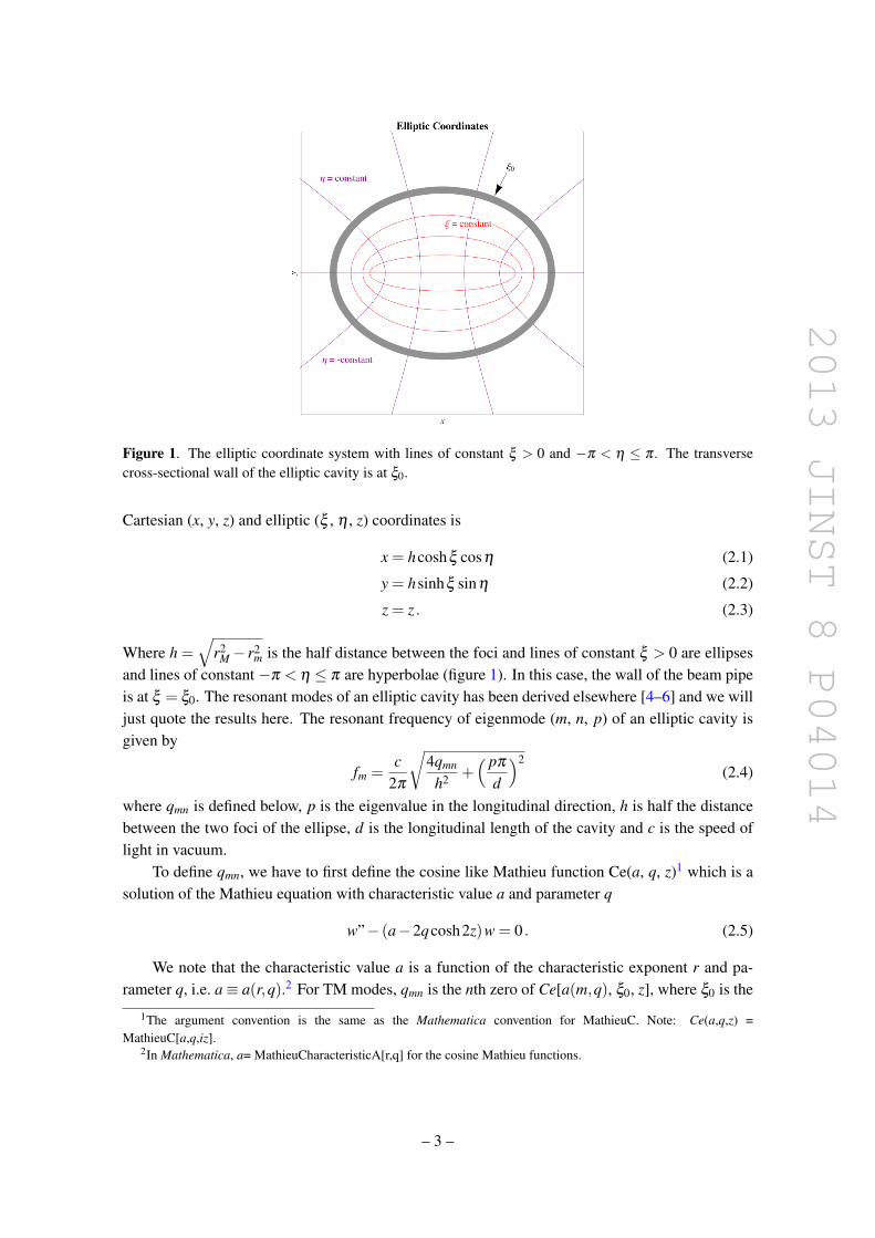
Figure 1. The elliptic coordinate system with lines of constant ξ > 0 and −π < η ≤ π . The transversecross-sectional wall of the elliptic cavity is at ξ0.

Cartesian (x, y, z) and elliptic (ξ , η , z) coordinates is

x = hcoshξ cosη (2.1)

y = hsinhξ sinη (2.2)

z = z . (2.3)

Where h =√

r2M− r2

m is the half distance between the foci and lines of constant ξ > 0 are ellipsesand lines of constant −π < η ≤ π are hyperbolae (figure 1). In this case, the wall of the beam pipeis at ξ = ξ0. The resonant modes of an elliptic cavity has been derived elsewhere [4–6] and we willjust quote the results here. The resonant frequency of eigenmode (m, n, p) of an elliptic cavity isgiven by

fm =c

2π

√4qmn

h2 +( pπ

d

)2(2.4)

where qmn is defined below, p is the eigenvalue in the longitudinal direction, h is half the distancebetween the two foci of the ellipse, d is the longitudinal length of the cavity and c is the speed oflight in vacuum.

To define qmn, we have to first define the cosine like Mathieu function Ce(a, q, z)1 which is asolution of the Mathieu equation with characteristic value a and parameter q

w”− (a−2qcosh2z)w = 0 . (2.5)

We note that the characteristic value a is a function of the characteristic exponent r and pa-rameter q, i.e. a≡ a(r,q).2 For TM modes, qmn is the nth zero of Ce[a(m,q), ξ0, z], where ξ0 is the

1The argument convention is the same as the Mathematica convention for MathieuC. Note: Ce(a,q,z) =MathieuC[a,q,iz].

2In Mathematica, a= MathieuCharacteristicA[r,q] for the cosine Mathieu functions.

– 3 –

2013 JINST 8 P04014

elliptic coordinate of the wall of the cavity, m = 0,1,2, . . ., and n = 1,2,3. . .. For TE modes, qmn

are the zeroes of Ce′[a(m,q), ξ0, z], where “′” is the derivative w.r.t. z.

2.2 Main Injector beam pipe cavity

We approximate the cross-section of the MI beam pipe with an ellipse and use the dimensions usedin the Microwave Studio simulation discussed in section 3.3 for calculating the resonant modes ofthe cavity. The length of the cavity is d = 1 m, the length of the semi-major axis is rM = 5.9 cmand the semi-minor axis is rm = 2.7 cm. Thus, the half distance between the foci is

h =√

r2M− r2

m = 0.052m . (2.6)

The elliptic coordinate ξ0 of the wall of the beam pipe comes from solving

x2

ρ2 cos2 ξ+

y2

ρ2 sin2ξ

= 1 (2.7)

for ρ0 and ξ0 given the lengths of the semi-major and semi-minor axes, i.e.

ρ0 cosξ0 = rM ρ0 sinξ0 = rm . (2.8)

Therefore, for the first approximation of the Main Injector beam pipe, we have ξ0 = 0.4943 rad.Using these dimensions, we find that the modes between 1.5 GHz to 2.5 GHz are all TE1,1,,n becausethe lowest TM mode TM0,1,0 is at 3.3 GHz and TE0,1,1 is at 1.5 GHz.

2.3 Frequency shift from the insertion of a piece of dielectric

The perturbation method for calculating the frequency shift from the insertion of a piece of dielec-tric into an RF cavity is well-known [9, 10]. Let us suppose that the piece of dielectric is at z = ze

and has thickness ∆ze. See figure 2. This means that both ε and µ behave as follows

ε =

{ε0 for z < ze and z > ze +∆ze

ε0

(1+ ∆ε

ε0

)for ze ≤ z≤ ze +∆ze

(2.9)

µ =

{µ0 for z < ze and z > ze +∆ze

µ0

(1+ ∆µ

µ0

)for ze ≤ z≤ ze +∆ze

(2.10)

If we assume that ∆ε/ε0� 1 and ∆µ/µ0� 1, so that both the electric fields E and magneticfields H are approximately equal to the unperturbed fields E0 and H0 respectively then we have

∆ω

ω0=

∫∆V dυ

(∆ε

⇀

E20−∆µ

⇀

H20

)∫

Vcdυ

(ε0

⇀

E20 + µ0

⇀

H20

) (2.11)

where the integral is over the volume Vc of the cavity, ∆ω = ωe−ω and ωe is the perturbed fre-quency and ω0 is the unperturbed resonant frequency. Eq. (2.11) is the result of Slater’s perturbationtheorem. Therefore, the frequency shift from a small piece of dielectric can be derived if

⇀

E0 and⇀

H0

are known. In fact, the TM fields of an elliptic cavity have already been derived by Yang [8], and itonly takes a little bit of work to get the TE fields. However, since eq. (2.11) has to be numericallyintegrated anyway, the formula is of academic interest only and will not be used in this paper.

– 4 –

2013 JINST 8 P04014

Figure 2. The measured modes using s21 and the calculated modes before and after fitting h and d tothe measured data from modes TE1,1,4 to TE1,1,13. The relative difference between the measured and thecalculated modes are all < 1% (see table 1).

Table 1. Elliptic modes of Main Injector cavity.

Mode Measured Calculated Fractional difference (%)TE1,1,1 1.5279 1.5253 -0.17TE1,1,2 1.5522 1.5472 -0.32TE1,1,3 1.5909 1.5832 -0.48TE1,1,4 1.6422 1.6321 -0.62TE1,1,5 1.7052 1.6930 -0.72TE1,1,6 1.7781 1.7646 -0.76TE1,1,7 1.8609 1.8456 −0.82TE1,1,8 1.9482 1.9349 -0.68TE1,1,9 2.0418 2.0314 -0.51TE1,1,10 2.1390 2.1340 -0.23

3 Numerical modelling

3.1 Phase shift of microwave traveling through a plasma gas (electron cloud)

In the experiment, a microwave signal is fed into the pipe through the probe of the coaxial couplerat one side of the pipe and detected by the 2nd probe at the other side. In the simulation, theyare modeled with discrete ports, as shown in figure 4. The entire system configuration has beensimplified to be the elliptical beam pipe blocked by the apertures that induce signal reflections atboth sides of the pipe. In electron gas diagnostics, the phase of a carrier signal, while travelingalong the beam pipe, is shifted by the presence of the electron cloud with gas density, n, which isgiven by

∆ϕ

L=

ω2p

2c√

ω2−ω2c

, (3.1)

– 5 –

2013 JINST 8 P04014

Figure 3. An x-ray view of the elliptical pipe resonator where a dielectric (shaded in cyan) with length ∆ze

has been inserted at z = ze.

and

ωp =

√nee2

ε0me

∼= 56.4√

ne (3.2)

where e is the electron charge, ε0 is the permittivity in free space, and me is the electron mass.Electron clouds energized by a proton beam are normally very dilute gas; densities range from1011–1012 m−3. The phase shift ratio (∆ϕ/L) of a traveling wave signal in the dilute gas would betoo small to be properly identified; even a 10 m long beam pipe may not enhance the phase shiftlarge enough to be clearly measured by a signal detector (antenna) within the phase resolution.Due to the nature of the single path interaction through the waveguide, traveling waves also havenearly zero response to localized gases, which have no variation on their phase shifts. Therefore,this method is also limited in identifying the spatial location of the electron cloud. On the otherhand, a cavity resonator captures waves of the spectrum between a waveguide cutoff and a cavitycutoff and the wave of a cavity eigenmode undergoes a large number of round-trips until it reachesa saturation point (RF filling time), which could remarkably increase a phase shift. Figure 4 showsthe conceptual drawing of the resonator electron cloud diagnostics. Multiple trips of a trappedeigenmode effectively increases the travel distance, L, which thereby enhances the phase shift,as depicted in eq. (3.1). The feeble phase shift through a dilute plasma gas can be thus rapidlyincreased far beyond the resolution limit of a signal detector within a very short distance. Besides,since cavity eigenmodes respond more or less sensitively to electron gases depending upon theirlocations corresponding to trapped waveforms, the technique might be much more efficient foraccurately specifying the spatial position and distribution of the electron cloud.

– 6 –

2013 JINST 8 P04014

3.2 Dielectric approximation of uniformly distributed electron gas

Electron Cloud (EC) simulations using Particle-In-Cell Codes (PIC) provide a powerful tool forunderstanding cloud build up and mitigation techniques, as well as traveling TE microwave diag-nostics of electron clouds. However, to explicitly model sidebands induced in TE waves due toelectron cloud plasma, one must simulate beam revolution time scales (the cloud modulation time)while still resolving the rf signal. Modeling electron clouds as kinetic particles is time consuming(particle pushes are slow compared to field updates) and numerically noisy over long simulationtimes (grid heating). One solution is to replace kinetic particles with an equivalent plasma di-electric model [11]. Plasma dielectric models of electron clouds are much faster, and are morestable numerically.

In the given experimental system, the beam pipe is assumed to be filled with an electron gas,with a density (n), produced by a high intensity proton beam. Although density distribution of areal gas state has a spatial dependence, n = n(r), for simplicity, we first consider a constant density,n = n0. A plasma gas with a constant density can be thus simply approximated as a dielectricmedium by a Drude model, as follows.

n =√

εµ , (3.3)

where

ε (ω) = ε0

(1−

ω2p

ω2

)and µ = µ0 (3.4)

This dielectric approximation very effectively reflects the typical response of a uniformly dis-tributed plasma gas since the gas strongly resonates with an incident wave as ω approaches ωp.Therefore, the electron cloud could be equivalently modeled with a dielectric medium with aneffective dielectric constant, n.

Figure 4 shows a signal processing algorithm from a microwave simulation to calculate aphase shift by an effective electron gas. The port-1 (source) generates a carrier signal of sinusoidalwaveform, S1(t) = A1 sin(ωt + ϕ1), where ϕ1 is the initial phase (ϕ1 = 0), that travels throughthe uniformly filled elliptical beam pipe. The detected signal at port-2 (antenna receiver) has thesinusoidal waveform of S2(t) = A2 sin(ωt + ϕ2ϕm), where ϕ2 is the initial phase and ϕm is the phasechange over the source-to-antenna distance with a dielectric constant, n. In order to extract a phasechange, ϕm, from the simulation, let us multiply S1 and S2,

S1S2 = A1A2 sin(ω1t)sin(ω2t +ϕm) . (3.5)

By trigonometric identity, eq. (2.5) becomes

S1S2 =A1A2

2[cos(ϕm)− cos(2ωt +ϕm)] (3.6)

where ω = ω1 = ω2.The second term in eq. (3.6), cos(2ωt + ϕm), can be removed by a low pass filter (LPF) of

a post-processor. The low pass filter process is precisely shown in figure 4. The S1S2, obtainedfrom field data monitored at the port-1 and –port2 in simulation, is decomposed into amplitude-and phase-spectra by fast Fourier transform (FFT). The 2nd frequency harmonic term (2ωt) is then

– 7 –

2013 JINST 8 P04014Figure 4. Conceptual flowchart of signal processing and computational algorithm to calculate phase-shifts

due to electron clouds from equivalent dielectric simulation models.

crossed out by low pass filtering. The inverse FFT of the LPF’ed amplitude and phase leaves onlythe cosine term of phase change. Therefore, the phase change, ϕm, is

ϕm = cos−1(

2×LPF(S1S2)A1A2

)(3.7)

The phase shift, ∆ϕ , by an electron cloud is ∆ϕ = |ϕe−ϕv|, where ϕe is the phase variation (ϕm)through the electron gas and ϕv is the phase variation (ϕm) through a vacuum filled in the beam pipe.This approximation is generally valid since A1 is constant and A2 is very slowly varying amplitude,which is nearly constant, in the time scale of signal frequency. Normally, in the simulation A1 canbe set to be a unity, so that A2 would need to be measured at a time of saturation (t = tsaturation).

– 8 –

2013 JINST 8 P04014

Figure 5. Finite-integral-technique (FIT) simulation models (a) elliptical waveguide and (b) elliptical cavity.Two discrete antenna ports for transmitting and receiving a carrier signal are located adjacent to the openboundaries in the beam pipe. The boundaries are programmed to meet perfect matching layers (PML). Thepipe material is designed with a stainless steel.

3.3 Waveguide and cavity resonator models

Applying the same analytic method, we compare the phase shifts of a traveling wave throughwaveguide and standing wave in a cavity resonator. Figure 5 shows the simulation models based onthe elliptical beam pipe: one has ears at both ends to trap waves propagating above the cutoff in thebeam pipe, whereas the other is connected only with the open boundary. The pipe length is set to be1 m and port-to-port distance (l) is 0.95 m. The upper cutoff frequency is determined by the widthof the aperture (gap spacing between the ears), which also determine the number of eigenmodescaptured in the cavity. The cross-sectional dimensions of the elliptical beam pipe are 11.8 cm(major) × 5.4 cm (minor), which corresponds to 1.516 GHz of beam pipe cutoff frequency ( fc).The model for the initial numerical analyses was designed to have 6 mm wide ears. Subsequently,however, the ears were re-designed to be 20 mm wide to examine the effect of leakage fields throughthe apertures since it was found that the beam apertures could be allowed to open up to 80 mm forthe proton beam.

As shown in figure 6, the 6 mm wide ear captures 3 resonating modes, (1) 1.5224 GHz (p =1), (2) 1.5416 GHz (p = 2), and (3) 1.573 GHz (p = 3), between the two cutoff frequencies of thebeam pipe and the aperture, 1.516 GHz and 1.974 GHz. The discrepancy between the measuredand theoretical frequencies listed in table 1 is attributed to the following reasons: the MI beam pipeis only approximately elliptical in cross section because it was made by squashing a circular beampipe. Also, the theoretical model is for a closed cavity, whereas the simulated one is based on openboundaries (apertures). Figure 6(b) shows field distributions of those eigenmodes with longitudinalphase changes of p = 1, 2 and 3. Note that the opening size of the apertures is comparable to

– 9 –

2013 JINST 8 P04014

Figure 6. (a) S21 spectrum measured at port-1 and -2. The designed beam pipe holds three resonatingmodes inside (b) field distributions of the three modes (π-mode of f = 1.5304 GHz is a carrier signal fortime-transient analysis.

Figure 7. Phase shift versus time graphs of waveguide (blue) and cavity (red) beam pipe models. The cavityenhances the phase-shift by a factor of 10. (ear length/width = 60 mm/6 mm)

the wavelengths, leading to a large leakage of fringe fields. Since the 3π mode (1.573 GHz) hasa maximum field amplitude at the aperture position (z = l/2), a huge amount of fringe fields isleaked out through the apertures. On the other hand, as depicted in figure 6(b), as the π-mode(1.5224 GHz) has a minimum field amplitude at the cavity fringes, thereby leading to a significantlysmaller amount of leakage fields. One can thus see that the π-mode would have a larger phase-shiftthan the 3π-mode, as shown in eq. (3.1). We choose 2π-mode (p = 2, 1.5416 GHz) to compare thephase shift of the cavity with that of the waveguide as the mode properly reflects the average phaseshift of the π- and 3π-modes.

Figure 7 shows the phase-shift versus time graphs of the cavity and waveguide models with the2π-mode carrier ( f = 1.5416 GHz), which was obtained from the numerical analysis depicted in2.2. For consistency, the models are simulated with the same condition, e.g., charge density, ne =

– 10 –

2013 JINST 8 P04014

Figure 8. (a) Phase shift versus time graph (b) electron cloud charge density versus time graphs fromtwo different assumptions on the wave traveling distance in the cavity: linear- (blue) and non-linear (red)increases.

1011 m3. The comparative analysis result ended up showing a noticeable improvement: phase shiftseems to be enhanced 10 times more by the cavity than the waveguide. In figure 7, the carrier signalin the waveguide quickly reaches the maximum phase shift (∆ϕ ∼ 2.3 mrad) at t = 2 µs. However,it continuously rises in the cavity beam pipe up to ∆ϕ ∼ 23 mrad until t = 6 µs when the cavityreaches a steady state. Ohmic losses and external coupling mainly constrain RF filling time in thecavity that determines the number of round trips (signal travel distance) required to reach a steadystate. A phase shift can be thus further increased with a cutoff-nearest mode (p = 1: fundamentallongitudinal mode), a high conductivity material and a smaller aperture on the beam pipe.

3.4 Electron cloud density calculation

In order to verify the proposed concept of the cavity resonator, we re-calculate the electron clouddensity from the cavity-enhanced phase shift of the simulation model. In principle, as a phaseshift increases with travel distance, a normalized phase shift should be the same with the samegas density at the steady state either in a cavity or in a waveguide: in eq. (3.1), gas density isthe function only of carrier frequency, cutoff frequency, and normalized phase shift, which has nodependence on the distance (L). We first assume that the travel distance linearly increases with time:L is assumed to be proportional to group velocity multiplied by time, L = υg·t. The group velocityis obtained by calculating a time-dependent signal profile. Figure 8 shows the time-dependentcharge density graph. The input parameters for the density calculation are given as the 2π-modecarrier frequency of f = 1.5416 GHz, fc = 1.516 GHz, and ne = 1011 m−3. The charge densitylinearly increases until t =∼ 2 µs and gradually decreases after the stationary state since the traveldistance of the carrier signal is assigned to continuously increase in the definition, whereas thephase shift is saturated after RF filling time. In other words, the phase shift is no longer increasedin the time period after a carrier signal of a cycle completely leaves from the resonator, even ifL is assumed to continue to increase in the analytic model. Figure 8(b) shows that the chargedensity at ∼ 2 µs, corresponding to the saturation time of phase shift in figure 8(a), is ∼ 1011 m−3,which is exactly matched with the theoretically pre-assigned density to the dielectric Drude modelof eqs. (3.3) and (3.4): one can see that the theoretical calculation based on the signal mixing

– 11 –

2013 JINST 8 P04014

technique accurately predicts the electron cloud density, represented with an equivalent dielectricmodel, in the cavity beam pipe. In order to compensate for the saturation effect, we neverthelessmodify the definition of the signal travel distance from a linear increment to one fitting the phase-shift curve in figure 8(a) to more accurately reflects the time-dependent pattern of charge density.The red curve in figure 8(b) is the corrected charge density versus time graph, which clearly showsthat the analytic curve converges to the defined density (1011 m−3). In this model, the incrementalrate of signal travel distance also gradually decreases with that of the phase shift. This calculationtechnique can thus provide an exact charge density after the simulation time of phase saturation.The comparative analysis verified that a cloud density can be still accurately calculated even fromthe enhanced phase-shift resolution of the cavity resonance diagnostics.

4 Parametric analysis

In principle, phase-shift enhancement of the cavity beam pipe is mainly determined by the amountof evanescent fringe fields through the apertures. It is understood that the smaller leakage fieldslead to the larger phase-shift enhancement over the longer saturation time as a trapped wave has alonger traveling time and distance with smaller external coupling losses. Basically, the phase-shiftis thus proportional to a cavity external Q (Qext). With respect to geometrical configuration of anopened cavity resonator, the amount of leakage fields through the coupling hole-apertures can bereduced by increasing the aperture length to increase Qext with a fixed width. However, the actualelectron cloud diagnostics apparatus in MI ring has the physical constraint to have long ears, so weinvestigated enhancement factors in terms of the ear length using our theoretical analysis. Figure 9shows phase-shift graphs in terms of the ear lengths that are calculated with the fixed ear width(= 20 mm) in figure 5(b). The width of the beam pipe aperture was chosen to be ∼ 80 mm withthe consideration of the maximum proton beam diameter. Sweeping the ear lengths ranges from25 mm to 150 mm with a 25 mm step. The phase-shift graphs in time domain clearly depicts that theshortest aperture with the longest penetration depth of an evanescent leakage field has the smallestphase-shift resolution with the short saturation time. The converging shift resolution is graduallyincreased from 8 mrad to 40 mrad as the saturation time moves from ∼ 2 µs to ∼ 8 µs, but it doesnot increase above the ear length = 125 mm as shown in figure 9(b). The beam pipe apertures with≥ 100 mm lengths appear to have significantly small amounts of external energy losses, whichthereby need a few thousand round trips for a π-mode standing wave to be completely coupledout with the 1 m long beam pipe cavity. As shown in figure 9(b), the saturated phase-shifts do notexceed ∼ 40 mrad as fringe fields at the apertures have a constant amount of leakage with the earlength of ≥ 100 mm. However, weakening the leakage fields is constrained by the aperture size,which is thereafter limited due to proton beam size.

5 Spatial identification of a localized electron gas

During its operation, the MI may experience irregular electron gas emissions from the proton beamowing to various unknown factors under the periodic magnetic confinement. Accurate diagnos-tics of spatiotemporal profiles of this un-controlled localization is one of the critical issues to beresolved. The standing wave characteristic of the resonating cavity technique may be capable of

– 12 –

2013 JINST 8 P04014

Figure 9. (a) Phase versus time graphs with respect to the ear lengths (b) saturated phase-shift versus ear-length graph (carrier signal: f = 1.5224 GHz, π-mode in figure 3(b)). z = 150 mm (red) is not fully saturatedin t = 10 µs.

providing spatial analysis of electron cloud density distribution. It is evident that a phase shiftvastly changes depending upon whether the localized electron gas is positioned at a node or ananti-node of a standing wave: in other words, phase change of a carrier signal is maximum withanti-nodes and minimum with nodes. Therefore, phase analysis of multiple carrier signals over thespectrum of resonating modes confined in the beam pipe cavity will make it possible to identifythe location and spatial distribution of electron clouds. Figure 7 shows phase-shift spectra (∆ϕ),between two cutoffs of the beam pipe and aperture, of the two beam pipe fully filled uniform gasand with localized gas, modeled with the 5 cm long dielectric block, and field (Ey) plots corre-sponding to individual resonating peaks. The dielectric constant of dielectric insertions is definedas ne = 1011 m−3 electron density. In order to clearly form a standing wave in the simulation, theaperture is designed with a very small width (5 mm) that traps a large number of resonating modesin the beam pipe. In figure 10(a), the maximum field positions of the peaks on the localized gasspectrum are all exactly matched with the dielectric position of z = 0 m. The other non-resonatingpeaks disappear. With z = 0.125 m, 0.25 m and 0.375 m in figures 10(b)–(d), one can see that thepeaks with anti-nodes closely matched with the dielectric positions remain on the localized gasspectrum whereas the other peaks with nodes matched with the positions appear to have nearlyzero phase shift, which thereby disappear in the spectra. Note that the lower frequency modes havelarger phase shifts with smaller spatial resolution, while higher frequency signals have better spa-tial resolution as phase shift becomes smaller with an increase of frequency. As the phase shift isalso proportional to a traveling distance, a localized gas thickness would thus need to exceed a cer-tain value to have distinct resonating peaks in the high frequency spectrum. However, overlappingthe field distributions of resonating modes will enable one to accurately conjecture a position ofelectron gas, including mapping a one-dimensional density distribution. Although these simulationresults verify the diagnostic method of microwave resonant cavity, more systematic investigationis still necessary to explore its feasibility for the spatial and temporal electron cloud mapping andis currently under development.

– 13 –

2013 JINST 8 P04014

(a)

(b)

– 14 –

2013 JINST 8 P04014

(c)

(d)

Figure 10. Phase shift spectra and eigenmode field plots of localized electron clouds with respect to theaxial positions of the equivalent model (electric insertion): (a) z = 0 m (b) z = 0.125 m (b) z = 0.25 m, and(d) z = 0.375 m.

– 15 –

2013 JINST 8 P04014

Figure 11. Phase shift due to 2.7 cm thick dielectric at the center of the new setup for 8.26 cm aperturewidth. The graph compares phase shift for three different thicknesses: 80 µm (negligible thickness), 2.1 cmand 4.3 cm. The phase signal is generally larger for thicker reflector.

6 Experimental test

In order to test the effectiveness of the reflector ‘ears’, we performed a series of bench-top experi-ment with the MI pipe of 1 m length and a cross section 11.8 cm by 5.4 cm. We set up the networkanalyzer to generate microwave signal with a frequency span from 1.5 GHz to 2.4 GHz with abandwidth of 10 kHz, and measure the phase of S21 transmission. Two 5.08 cm half-wave dipolesin transverse orientation are used to transmit and receive even TE11 mode with cutoff frequency ataround 1.516 GHz. To model the e-cloud, we placed the 2.7 cm dielectric (Teflon) at the center ofthe waveguide. The phase data were collected with and without the dielectric inside the waveguide.We calculated the phase shift of the signal due to the dielectric by subtracting the phase data withoutthe dielectric from the phase data with the dielectric. Reflectors of three different thickness, 80 µm,2.1 cm, and 4.3 cm, were designed. The aperture was set to 108 mm as mentioned in figure 5(b).Figure 11 shows the phase-shift due to three different reflector thicknesses. As predicted by thesimulation, the thicker the reflector-ears, the higher the phase-shift. A separate experiment usingdistributed dielectric also indicates phase-shift improvement when thick ears are used as reflectors.

7 Conclusion

We have developed an effective method to accurately measure the density of dilute electron cloudsgenerated by high intensity proton beams. The strong phase shift enhancement from multiple re-flections of standing waves in a resonating beam pipe cavity has been demonstrated with numericalmodeling using dielectric approximation and microwave S-parameter measurements. The equiva-lent dielectric simulation showed a ∼ 10 times phase shift enhancement (2π-mode, 1.5416 GHz)

– 16 –

2013 JINST 8 P04014

with the cavity beam pipe compared to the waveguide model. The position-dependence of the tech-nique is investigated by overlapping the field distributions of harmonic resonances. The simulationwith various positions of dielectric insertions confirmed that resonance peaks in phase-shift spec-tra corresponding to the relative distance between field-nodes and electron cloud position, whichallows for one-dimensional mapping. Preliminary experimental studies based on a bench-top setupconfirm the simulation showing that thicker reflectors enhance the phase-shift measurement of theelectron cloud density.

Acknowledgments

We would like to acknowledge B. Fellenz for the support of the experiment. We also thank the LeeTeng interns Hexuan Wang and Phyo Kyaw for the experimental work on the prototype.

References

[1] S. Nagaitsev, Project X - New Multi Megawatt Proton Source at Fermilab, at PAC’2011 conference,New York U.S.A. (2011), FROBN3.

[2] S. De Santis et al., Measurements of the Electron Cloud in Large Accelerators By MicrowaveDispersion, Phys. Rev. Lett. 100 (2008) 094801.

[3] R. Zwaska, Electron cloud experiments at Fermilab: formation and mitigation, Conf. Proc. C110328(2011) 27, PAC-2011-MOOBS4, FERMILAB-CONF-11-081-APC.

[4] S.De Santis et al., Analysis of Resonant TE Wave Modulation Signals for Electron CloudMeasurements, in Proceedings of International Particle Accelerator Conference 2012, New OrleansU.S.A. (2012).

[5] J.P. Sikora et al., Using TE Wave resonances for the Measurement of electron cloud density, inProceedings of International Particle Accelerator Conference 2012, New Orleans U.S.A. (2012).

[6] A. Pietropaolo et al., DINS measurements on VESUVIO in the resonance detector configuration:proton mean kinetic energy in water, 2006 JINST 1 P04001.

[7] A.I. Harris, Spectroscopy with multichannel correlation radiometers, Rev. Sci. Instrum. 76 (2005)054503 [astro-ph/0504449].

[8] G.F. Knoll, Radiation detection and measurements, John Willey and Sons Inc., New York U.S.A.(2000).

[9] L.C. Maier and J.C. Slater, Field Strength Measurements in Resonant Cavities, J. Appl. Phys. 23(1952) 68.

[10] L.B. Mullet, G/R.853, Atomic Energy Research Establishment, Harwell U.K. (1952).

[11] S.A. Veitzer, D.N. Smithe and P.H. Stoltz, Application of new simulation algorithms for modeling rfdiagnostics of electron clouds, AIP Conf. Proc. 1507 (2012) 404.

– 17 –