theory open-ended circular cylindrical microwave cavity · the open-ended microwave cavity ... (ic)...

c .

N A S A TECHNICAL NOTE NASA TN D-3514

* CI

un - GPO PRICE S d .

U C C E S S I O N NUWBERI WHRUI .. N66 30om f P

z

>

(=OTO 3 a

~CATLOORI) -A CR O R TMX O R AD NUMBER)

THEORY OF OPEN-ENDED CIRCULAR CYLINDRICAL MICROWAVE CAVITY

by Norman C.

Lewis Research Clevektnd, Ohio

Wenger Center

NATIONAL AERONAUTICS AND SPACE ADMINISTRATION WASHINGTON, D. C. JULY 1966

https://ntrs.nasa.gov/search.jsp?R=19660020790 2018-06-29T18:19:22+00:00Z

NASA TN D-3514

THEORY OF OPEN-ENDED CIRCULAR CYLINDRICAL

MICROWAVE CAVITY

By Norman C. Wenger

Lewis Research Center Cleveland, Ohio

NATIONAL AERONAUTICS AND SPACE ADMINISTRATION

For sale by the Clearinghouse for Federal Scientific and Technical Information Springfield, Virginia 22151 - Price $2.00

i

I

' *

t CONTENTS

Page SUMMARY . . . . . . . . . . . . . . . . . . . . . . . . . . . . . . . . . 1

INTRODUCTION . . . . . . . . . . . . . . . . . . . . . . . . . . . . . . 1

SYMBO . . . . . . . . . . . . . . . . . . . . . . . . . . . . . . . . . . . 3

WAVEGUIDE MODES . . . . . . . . . . . . . . . . . . . . . . . . . . . . 4 Region1 . . . . . . . . . . . . . . . . . . . . . . . . . . . . . . . . 4 RegionII . . . . . . . . . . . . . . . . . . . . . . . . . . . . . . . . 6 Region I D . . . . . . . . . . . . . . . . . . . . . . . . . . . . . . . . 6

SOLUTION FOR REFLECTION COEFFICIENT. . . . . . . . . . . . . . . . . 7 Integral Equation for Electric Field . . . . . . . . . . . . . . . . . . . . 7

Green's function . . . . . . . . . . . . . . . . . . . . . . . . . . . . 8 Electric field . . . . . . . . . . . . . . . . . . . . . . . . . . . . . 10 Integral equation . . . . . . . . . . . . . . . . . . . . . . . . . . . . 10

Solution of Integral Equation . . . . . . . . . . . . . . . . . . . . . . . 13 Laplace transforms . . . . . . . . . . . . . . . . . . . . . . . . . . 13 Wiener-Hopf technique . . . . . . . . . . . . . . . . . . . . . . . . . 15 Edge conditions . . . . . . . . . . . . . . . . . . . . . . . . . . . . 17 Wiener-Hopf factors of Green's function . . . . . . . . . . . . . . . . . 17 Scattered electric field . . . . . . . . . . . . . . . . . . . . . . . . . 21

Reflection Coefficient . . . . . . . . . . . . . . . . . . . . . . . . . . 23

RESONANT FREQUENCY OF CAVITY . . . . . . . . . . . . . . . . . . . . 26

CONCLUSIONS . . . . . . . . . . . . . . . . . . . . . . . . . . . . . . . 28

REFERENCES . . . . . . . . . . . . . . . . . . . . . . . . . . . . . . . 29

I .

I

Microwave cavities have been used for a number of years to measure the relative dielectric constants of gases (refs. 1 to 3). The relative dielectric constant is given by the square of the ratio of the resonant frequency when the cavity is evacuated to the resonant frequency when filled with gas.

In many applications, such as in atmospheric research (ref. 4), it is desirable to make dynamic measurements of the dielectric constant by having the gas pass through the cavity. This requires replacing the solid end walls of the cavity by a termination

,

I


by Norman C. Wenger

Lewis Research Center

SUMMARY

The moll mode of oscillation in an open-ended circular cylindrical microwave I I

I cavity is discussed. The cavity consists of a circular waveguide terminated at each end with a thin cylindrical partition coaxial with the circular waveguide. The resonant frequency of the cavity is computed by using Laplace transform and Wiener-Hopf techniques. Numerical values for the resonant frequency are presented.

I

1

I

9

Figure 1. - Open-ended microwave cavity. ~ -

tions are sufficiently long. The cross- sectional obstruction of the terminations for this type of cavity is a result entirely of the finite wall thickness of the partitions plus any supporting structure. A cross- sectional obstruction of less than 2 percent of the end a rea has been reported (ref. 7). ,Z

7 . n - - Figure 2 -Cylindrical partition in waveguide. -

The open-ended microwave cavity shown in figure 1 was recently developed

at the Lewis Research Center to measure the density of liquid hydrogen under flow conditions. The density of liquid hydrogen can be computed from its relative dielectric constant by using an equation such as the Clausius-Mossotti equation. The cavity consists of a circular waveguide terminated at each end with a coaxial cylindrical partition. The effect of the cylindrical partition is to separate a portion of the waveguide into a coaxial waveguide plus a smaller circular waveguide that also serves as the inner conductor for the coaxial waveguide.

This report presents an analysis of open-ended circular cylindrical cavities of the type shown in figure 1 to determine the relation between the resonant frequency and the cavity dimensions for the case where the cavity is evacuated. The analysis is restricted to the TEOll resonant mode since this mode of oscillation has a very high Q and therefore is widely used. The solution for the resonant frequency of the TEOll mode can be easily computed if the reflection coefficient of the TEOl circular waveguide mode incident on the cylindrical partition is known.

The various regions of interest have been numbered for ease in reference. The model consists of a perfectly conducting circular waveguide of radius b and of infinite extent in the z-direction. Coaxial with the waveguide is an infinitely thin, perfectly conducting circular waveguide of radius a that extends over the range 0 < z < 00. The reflection coefficient will be computed for the case of the TE

The model that will be used to compute the reflection coefficient is shown in figure 2.

mode incident from the left. 01

2

Before proceeding with the analysis, it will be instructive to consider the various types of waves that can exist in the different regions. It will only be necessary, however, to consider the circularly symmetric "Eon modes since both the TEol incident mode and the model possess circular symmetry. Thus, the field components of interest will be the 8-component of the electric field and the r- and z-components of the magnetic field. All other field components will vanish.

SYMBOLS

radius of c i r c d a r partition (fig. 2)

radius of circular waveguide (fig. 2)

velocity of light

8 -component of electric field

8 -component of incident electric field

8 -component of scattered electric field

bilateral Laplace transformation of E:

singIe-sided Laplace transformation of E: over the interval z > 0

single-sided Laplace transformation of E: over the interval z < 0

Green's function

bilateral Laplace transformation of G(ry a, z)

Wiener-Hopf factor of y(a, a, B)

Wiener-Hopf factor of Y(a, a, 8) r-component of magnetic field

z-component of magnetic field

imaginary part of

8-component of electric surface current density on surface r = a for z > 0

J-1 bilateral Laplace transformation of J8

free-space wave number

3

L

P(P)

R

IR

rO

r

9 e

t

z

Z

a! 0

n P

pn

4 0;'

'n

yn

6n e

x

P O

Pn cp

w

, i

(ref.

4

length between partitions (fig. 6)

function of p that gives 9' and 9- proper behavior as ( P I - 00 reflection coefficient of TEOl mode

modulus of reflection coefficient

radial coordinate (fig. 2)

dummy coordinate

real part of

time

axial coordinate (fig. 2)

dummy coordinate

propagation constant of TEon mode in region I1

Laplace transformation variable

propagation constant of TEon mode in region I

real part of p,

negative imaginary part of 0, eigenvalue of TEon mode in region I

eigenvalue of TEon mode in region 11

eigenvalue of TEon mode in region 111

polar angle (fig. 2)

(k; + p y 2 magnetic permeability of free space

propagation constant of TEon mode in region 111

phase of reflection coefficient

angular frequency

WAVEGUIDE MODES

Region I

The general solution for the electromagnetic field in region I is of the form 8, pp. 69 to 72)

1 n= 2

I

where the 41 are complex amplitude constants. A time dependence of .jut is implicit in these equations. The propagation constants pn must satisfy the equations I

I

I where ko w/c, since the general solution must satisfy Maxwell's equations. The eigenvalues I'n are determined by the boundary condition that requires Ee(r, z) to vanish at the perfectly conducting surface r = b (see fig. 2). Thus, I

Jl(rnb) = 0 (3)

I which has the roots r l b = 3.8317, r 2 b = 7.0156, . . . , r b M (n + 1/4)n (ref. 9, I I p. 166).

The first two terms in the solutions (la) to (IC) are recognized as the incident and reflected mol circular waveguide modes, respectively, where R is the reflection coefficient. The remaining terms correspond to the 'Eon circular waveguide modes. It has been assumed that ko is in the range rl < ko < r2 so that the "Eol mode is a Propagating mode and the TE, (n > 1) modes are evanescent or cutoff modes.

5

Region I1

The general solution for the electromagnetic field in region 11 is of the form (ref. 8, pp. 69 to 72)

M

- CYnz Hr(r, z) = -) -, !?fh Jl(ynr)e

j w o n= 1

n= 1

where the Bn are complex amplitude constants. Since the general solutions must satisfy Maxwell's equations, the an are given by

2 - 2 2 an - Yn - ko

I

* I

(5)

The eigenvalues y, are determined by the boundary condition that requires Ee(r, z) to vanish at r = a (see fig. 2). Thus,

which has the roots yla = 3.8317, y2a = 7.0156, . . . , y, a M (n + 1/4)n (ref. 9, p. 166).

It has been assumed that ko is less than y1 so that all the TEon modes in region 11 are cutoff modes.

The terms in the solution are recognized as the TEon circular waveguide modes.

Region I11

The solution for the electromagnetic field in region 111 is of the form (ref. 8, pp. 77 to 80)

6

i - I

n= 1

n= 1

I

I where the C, are complex amplitude constants. The condition that the solution must I satisfy Maxwell's zquations requires

2 2 2 Pn = bn - ko

The boundary conditions require Ee(r, z) to vanish at r = a and r = b (see fig. 2). The

condition at r = b requires the eigenvalues 6n to satisfy the equation I boundary condition at r = a is satisfied automatically by equation (7a). The boundary I I I

j The roots of this equation are dependent on the ratio b/a. For example, if b/a = 1.2, tjla = 15.7277, b2a = 31.4259, . . . , 6na = nz&b/a) - l](ref. 9, p. 204).

The te rms in solution (7) correspond to the "Eon coaxial waveguide modes. It has been assumed that ko is less than 61 so that all the TEon modes in region III are cutoff modes.

I

t

I

SOLUTION FOR REFLECTION COEFFICIENT

Integral Equation for Electric Field

Since the electric and magnetic fields are related by Maxwell's equations, only the

7

electric field needs to be determined to specify the total field uniquely. Thus, the 8-component of the electric field, which is the only nonvanishing component of the electric field, can be regarded as a potential function from which the magnetic field components can be derived.

an integral equation for the scattered electric field due to the TEOl mode incident on the cylindrical partition.

Green's function, G(r, ro, z-zo), defined to be the solution of the differential equation

The formal solution for the reflection coefficient R will be obtained by setting up

Green's function. - The integral equation will be formulated by employing the

a2G 1 aG+aZG 6(r - ro) - + - - - + (kz - $G= -6(z - z0) rO

2 az ar2 r ar

that satisfies the boundary condition

G(b, ro, z-z ) = 0 (1 1) 0

The Green's function can be thought of as being the 8-component of the electric field radiated from a filamentary loop antenna of radius ro located at z = z long circular waveguide of radius b.

technique. A general solution of equation (10) that satisfies boundary condition (11) is of the form

in an infinitely 0

The solution for the Green's function will be obtained by using a mode-expansion

n= 1

where the Dn are expansion coefficients to be determined, and the rn are given by equation (3).

Substituting the general solution into equation (10) gives

n= 1

8

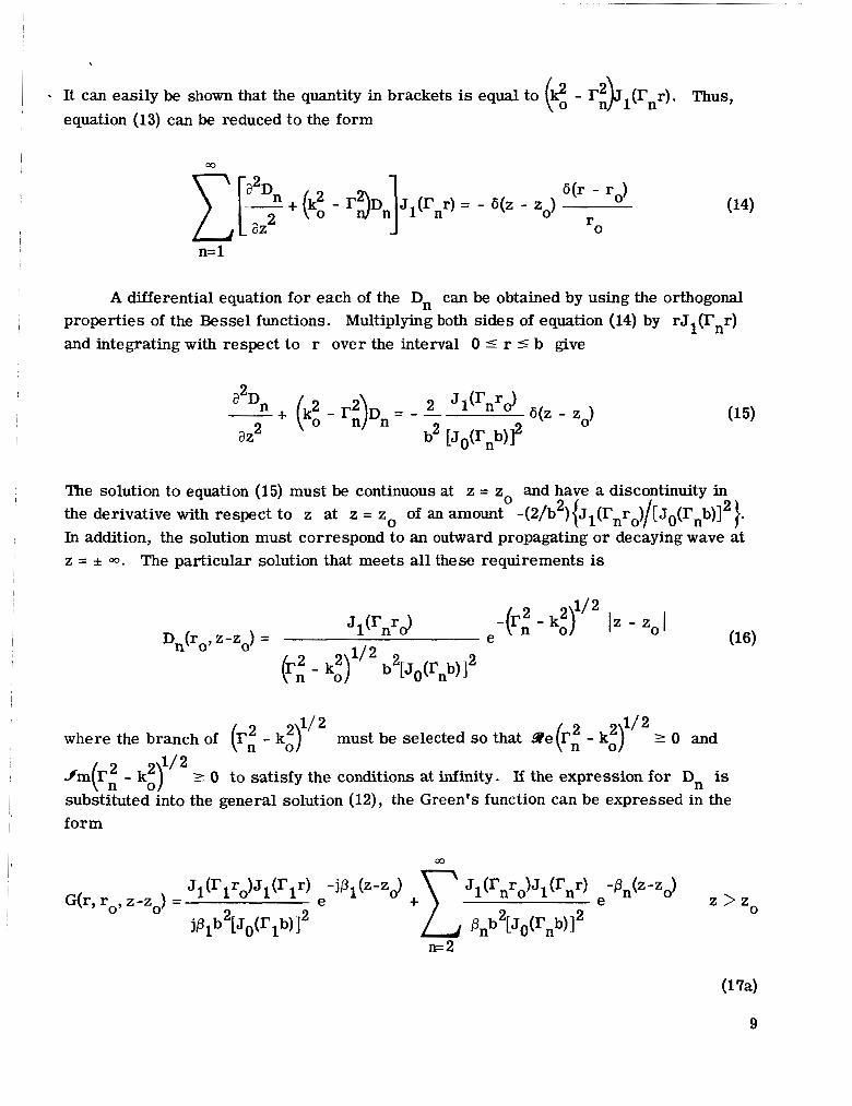
- It can easily be shown that the quantity in brackets is equal to (g - l?:)J1(rnr). Thus, equation (13) can be reduced to the form E[!% + (."o - I'>n]Jl(rnr) = - 6(z - zo) 6(r - ro)

az rO

n= 1

A differential equation for each of the D, can be obtained by using the orthogonal properties of the Bessel functions. Multiplying both sides of equation (14) by rJl(rnr) and integrating with respect to r over the interval 0 5 r 5 b give

J (r r J 6(z - zo)

a2Dn - + (kz - r:)Dn = - - 2 az

The solution to equation (15) must be continuous at z = zo and have a discontinuity in the derivative with respect to z at z = zo of an amount -(2/b2){Jl(rnro)/[Jo(I'nb)]2}. In addition, the solution must correspond to an outward propagating or decaying wave at z = f m. The particular solution that meets all these requirements is

1/ 2 must be selected so that ae(r: - kz) 1. 0 and

1/ 2 where the branch of (r: - ki)

1/ 2 .fm(m2 - k:) 1 0 to satisfy the conditions at infinity. If the expression for Dn is substituted into the general solution (12), the Green's function can be expressed in the form

9

As Iz - zo I becomes large, the value of G is given by the first term in either I equation (17a) or (1%). I

Electric field. - The 0 -component of the electric field Ee(r, z) must satisfy the differential equation ,

2 r ar az 2 + ( ko - -$Ee = 0

1 aEe +--- +- r ar

and the following boundary conditions (see fig. 2): I

Ee(b, z) = 0 all z (194

Ee(a, Z) = 0 for z > 0 (19b)

In addition, the electric field must correspond to the incident TEOl mode as z - -00. Thus,

-jP 1z lim Ee(r,z) = J l ( r l r ) e

Z-P-00

The reflected TEOl mode does not appear in equation (20) since it will later be assumed that the medium within the waveguide has small electrical losses so that the reflected field will have a negligible amplitude at z = -m.

then subtracting give Integral equation. - Multiplying equation (10) by Ee and equation (18) by G and

10

where

I S s2

I - 2 2 - 0

Figure 3. - Surface S.

2 a2 1 a 1 a2 a2 a r 2 ar r2 ae2 az

v = - +--+-- +- 2

Next, each term in equation (21) will be inte- grated over the volume V bounded by the surface S, as shown in figure 3. The various

portions of the surface have been denoted SI to S6 for ease in reference. The sur-

faces S1, S5, and S6 are at infinity. Performing the integration over the volume V gives

J (EeV2G - GV%e)dV = -bEe(ro , z0) V

The integral over the volume V can be reduced to an integral over the closed bounding surface S by using Green’s theorem (ref. 10, pp. 803 and 804) with the result

dS = -2nEe(ro, z0) an

where n is the outward normal coordinate to the surface S.

(boundary conditions eqs. (11) and (19a)) the portion of the surface integral over S2 will vanish. The surface integral over S5 and S6 will also vanish since Eo is zero at z = +m due to all the TEon modes in regions 11 and III being cutoff modes. In addition, the first term in the surface integral must vanish along the surfaces S3 and S4 since Ee is zero along the perfectly conducting surface r = a for z > 0 (boundary condition eq. (19b)). Thus, the only contributions to the surface integral will come from the integration over S1 and from the second term in the integrand over S3 and S4.

It can easily be shown by using the asymptotic forms of Ee and G as z - -00

Since both Ee and G are zero along the perfectly conducting surface r = b

-16 lzp that the integral over the surface S1 is equal to -2nJl(rlro)e faces S3 and S4, the quantity aEe/an is equal to -aEe/ar and aEe/ar, respectively. Equation (23) can therefore be expressed in the following form:

. Along the sur-

11

In order to simplify the form of equation (24), the function Jo(a, z) will be defined as

It can be easily shown by using Maxwell's equations that Je (a, z) is the electric surface current density on the surface r = a for z > 0. The value of Je(a, z) is zero, of course, for z < 0. Thus, equation (24) can be rewritten in the form

where r has been interchanged with ro, and z with zo for clarity. The symmetry property of the Green's function G(a, r, zo-z) = G(r, a, z-2,) (see eqs. (17)) was used to obtain equation (26)). Equation (26) shows that the total electric field Ee is the sum of the TEOl mode incident field given by the first term on the right plus an integral that corresponds to the field radiated by the electric current on the surface r = a for z > 0.

two parts: an incident field E: and a scattered field E: so that It will be convenient in the following analysis to split the electric field Ee into

E6(r, z) = Ei( r , z) + E:(., z) (2 7)

where

12

- jP 1z E;(r, z) = J l ( r l r ) e

I I . Combining equations (26) to (28) gives the desired integral equation for the scattered

electric field E;:

I

1 I

In going from equation (26) to equation (29), the lower limit on the integral was changed from 0 to -00 since J,(a, z d is zero in the range -00 < zo < 0.

I

Solution of Integral Equation

Laplace transforms. - The solution of the integral equation for the scattered electric field will be obtained by using Laplace transform and Wiener-Hopf techniques. Let the functions g(r, p),g(r, a, p), and /(a, p ) be the bilateral Laplace transforms with respect to z of E:(r, z), G(r, a, z), and Je(a, z), respectively:

In order to make all the Laplace transforms exist in a common region in the complex &plane, the propagation constant 8, will be made complex. This is equivalent

I to introducing an energy loss mechanism into the medium interior to the waveguide. Let I P1 = 0; - j/3? where p i > 0 and s;' > 0. In the final solution, B;' will be set equal to

zero to recover the solution for the lossless case. The functions k and / are, at this point, unknown since E: and Je are un-

known. However, it can be shown by using the expressions for the general forms of the solutions given by equations (l), (4), and (7) that 8 is analytic in the strip -p;'<S&?p<p;' and that / is analytic in the region 9e@ > 43;.

form of the solution for G given by equations (17). This approach will yield the trans-

I

l

The transform of the Green's function can be computed at once by taking the trans-

13

formed Green's function in the form of an infinite series. It will be more convenient in the following analyses, however, to compute the Green's function by first transforming the basic equation and boundary condition for the Green's function given by equations (10) and (11) and then solve the transformed equations. This approach will yield the solution for the transformed Green's function in closed form.

The Laplace transforms of equations (10) and (11) are

where the variable ro has been set equal to a to conform with equation (30b). It should be noted that the transform of G is taken with respect to z with zo = 0. The solution of equation (31a) that is bounded in the interval 0 5 r 5 b and satisfies equation (31b) is of the form

I

I I

9(r, a, P ) = A(a, P)J1(Xr) r 5 a (324 I

1/2 where A = (k2 +$) .

the right side of equation (31a), which requires 9 to be continuous at r = a and to have a discontinuity in the first derivative with respect to r at r = a of an amount -l/a. Solving for A and B and then substituting the results into equations (32) give

0 The functions A(a, P ) and B(a, P) are determined from the conditions imposed by

Since Y is an even function of A, the choice of either branch of h will yield the same result for 9. It can be shown that 9 is analytic in the strip -Py <geP < Py.

The Laplace transform of the integral equation for the scattered electric field given by equation (29) is

14

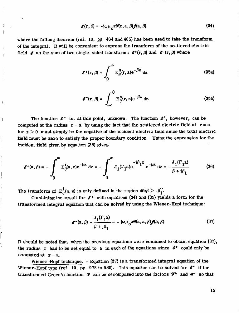
where the faltung theorem (ref. 10, pp. 464 and 465) has been used to take the transform of the integral. It will be convenient to express the transform of the scattered electric field 8 as the sum of two single-sided transforms Q+(r, B) and &(r, @) where

g+(r, @) = 4 Eg(r, z)e-Bz dz

0 8-(r, B) = [ E:(r, z)e-" dz

(354

The function Q- is, at this point, unknown. The function 8+, however, can be computed at the radius r = a by using the fact that the scattered electric field at r = a for z > 0 must simply be the negative of the incident electric field since the total electric field must be zero to satisfy the proper boundary condition. Using the expression for the incident field given by equation (28) gives

The transform of Et(a, z) is only defined in the region SPeB > -By. Combining the result for Q+ with equations (34) and (35) yields a form for the

transformed integral equation that can be solved by using the Wiener-Hopf technique:

It should be noted that, when the previous equations were .combined to obtain equation (37), the radius r had to be set equal to a in each of the equations since k+ could only be computed at r = a.

Wiener-Hopf technique. - Equation (37) is a transformed integral equation of the Wiener-Hopf type (ref. 10, pp. 978 to 980). This equation can be solved for 4' if the transformed Green's function Y can be decomposed into the factors Y+ and !T so that

15

Y = 9+/Y-, where 9+ is analytic and nonzero for 9 e p > -py and 9- is analytic and nonzero for 9eP < p;. This step allows equation (37) to be rewritten in the form

The left side of equation (38) is analytic in the region 9eP < 6;' except for the pole at P = -jPl introduced by the second term, whereas the right side of equation (38) is analytic for 9ep > -p;. The left side can be made analytic everywhere in the region 9?ep < Thus,

by adding the term [Jl(rla)9-(a, a, -jPl)]/@ + jp,) to each side of the equation.

Now, the left side is analytic for 9ep < p;' and the right side is analytic for 9 e p > -P;'. The equality in equation (39) holds only in the strip -P; < 9 e p < p;.

A function f l p ) can be defined from equation (39) so that .F(p) is equal to the left side of equation (39) for g e p 5 - f l y , the right side for 9 e P 2 B y , and to either side in the strip, -Pl <9ep < P,. Thus, 9@) is analytic everywhere in the finite complex P-plane.

It can be shown by using the asymptotic expressions for &'-,/,9+, and 9- for large P , derived in the following section, that F@) must also approach zero as p - m.

Consequently, F(/3) must be zero everywhere since zero is the only function that is analytic everywhere and vanishes at infinity (Liouville's theorem). Since .F@) is zero, each side of equation (39) must also be zero. Thus,

1 1 1 1

16

Edge conditions. - The conditions that have been specified for @ and Y- are that Y= @/Ye, Y+ be analytic and nonzero for 9e/3 > -By, and 9- be analytic and nonzero for ae/3 < py. These conditions do not uniquely specify this pair of functions since both g+ and 'T can be multiplied by any function that is analytic and nonzero everywhere in the finite p-plane to yield a new pair of functions that will satisfy all the original conditions. Any such pair of functions when combined with equations (40) will yield a solution for the scattered electric field that satisfies all the conditions imposed on the field up to this point.

The remaining boundary condition that must be imposed to specify the field uniquely is commonly called the edge condition (ref. 11). The edge condition reNres the total electric field Ee when evaluated at r = a to be of the order z112 as z - 0. The edge condition also requires the current density Je to be of the order z -112 as z - 0 .

Equation (28) shows that the incident electric field E: is of order 1 as z - 0 . Thus, the scattered electric field must also be of order 1 as z - 0 since the scattered field must have a component of this order to nullify the effect of the incident field so that the total field can be of the order z1/2 as z - 0 . The edge conditions can therefore be stated as

E:(a, z) = U(1) z - 0 (4 14

It can be easily shown that, if a function is of the order za! as z - 0 (a! >-1), its Laplace transform with respect to z will be of the order /3- (@+I) as /3 - 00. Con- sequently, the edw conditions require the transformed quantities 8- and / to satisfy the conditions

Combining equations (40) and (42) reveals that the functions @ and g- must be of

Wiener-Hopf factors of Green's function. - The transformed Green's function eval- the order 0- 1/2 and /3112, respectively, as 1/31 - 00. uated at r = a is given by (see eq. (33))

(4 3)

17

1/2 where h = (ki + 3) . The decomposition of 9 into the ratio of 9+ to 9' is best carried out 'by expressing '3 in the form of an infinite product.

The infinite product expansion of Jl(ha)/Aa is given by (ref. 10, pp. 382 to 385): =n n= 1

(44)

since the function Jl(ha)/ha is equal to 1 at h = 0, has a zero derivative with respect to h at A = 0, and has simple zeros at h = fyn (see eq. (6)). The infinite product expansion of J1(hb)/hb can be obtained from equation (44) simply by replacing a with b and yn with rn. Thus,

The infinite product expansion of the function J1(hb)N1(Aa) - J1@a)N1(Xb) is given by

J1(hb)N1(Xa) - J1(Xa)N1(Xb) =

since this function is equal to 2/n(b/a - a/b) at h = 0, has a zero derivative with respect to h at h = 0, and has simple zeros at A =

Combining equations (44) to (46) reveals that the transformed Green's function can be written in the infinite product form

(see eq. (9)).

[-$q-;) n= 1

n= 1

1 (4 7)

Equation (47) can be put into a more useful form by reintroducing the parameters On, cyn, and pn from equations (2), (5), and (8), respectively. Thus,

18

Equation (48) shows that the transformed Green's function has simple zeros at = fan and 8 = ipn and simple poles at P=*jPl and p = *B,(n > 1). Each of the infinite products can now be easily factored into the product of two infinite products so that one infinite product is analytic and nonzero in the region sPej3 < @;, and the other is analytic and nonzero in the region 9efi > -8;. The result of this operation allows and 9- to be easily identified as

2 2 The quantity 1 - a /b has been arbitrarily associated with the factor Y+. The exponential t e rms in equations (49) were introduced to make the infinite products converge. The logarithmic derivative of each of the infinite products generates an infinite series. If the exponential terms were absent, the nth term in each series would be of the order of l/n; consequently, each series and the associated infinite products would diverge. The exponential t e rms require the nth term of the series to be of the order of l / n , which ensures that both the infinite series and infinite products will converge. The form of these exponential t e rms is not unique since they are only required to generate

2

19

terms of the order l /n that will exactly cancel the existing terms of order l /n in the infinite series .

9'- the proper algebraic behavior for large 6, as discussed in the previous section. In order to solve for p(P) it will be necessary to determine the asymptotic forms of the infinite products for large P.

The function p(P) in equations (49) must be selected to give the functions Y+ and

Consider the infinite product

(%$)e-Pa/nn

n= 1

Since an and yn approach ns/a as n -. 00, it is apparent that the infinite product

only differs from the previous infinite product by a bounded function of P. Consequently, the asymptotic forms of the previous two infinite products will be identical for large

The gamma function r(x) can be expressed in infinite product form as (ref. 10, pp. 421 and 422)

M

where y is Euler's constant (y = 0.5772157.. .). The asymptotic form of r(x) is (ref. 10, p. 424)

r (x) (2A) 1/2 xx-(1/2),-x

as x - 00. Combining equations (50) and (51) shows that

20

. as x - 00. Thus, the initial infinite product

00

is of the order

as 0 - 00. This same procedure can be applied to each of the infinite products appearing in equations (49) with the result

as j3 - 00, and

as 0 - -00. Since g+ and g- must be of the order of #1-1/2 and $/2, respectively, as - it is apparent from equations (53) that a suitable choice for p(j3) is

Thus, the solution for the Wiener-Hopf factors of the transformed Green’s function is completed.

be computed by inverting the transformed field k : Scattered electric field. - The scattered electric field evaluated at r = a can now

2 1

The inversion contour C must be located in the I

strip -py <9ep < py, as shown in figure 4, since this is the only common region in the &plane in which all the transforms are analytic.

The transformed field ,$(a, p) is the sum of P ( a , P) given by equation (36) and 8-(a, 0) given by equation (40a). Combining equations (36) and (40a) with equation (55) gives

Figure 4. - Complex p-plane.

To evaluate the field for z < 0, the contour C can be closed in the right half P-plane with a semicircle of infinite radius, as shown in figure 4. It can be easily shown that the integral over this semicircle is zero. Thus, the integral over the original contour C must equal -2xj times the sum of the residues of the poles of the integrand in the right half &plane. The integrand has poles in the right half @-plane due to the zeros of 9- at /3 = jp, and at 0 = P,(n > 1). Performing the integration gives

Comparing equations (la) and (57) shows that the first term in equation (57) corresponds to the reflected TEOl mode, and the terms in the summation correspond to the evanescent TEon(n > 1) modes.

&plane with a semicircle of infinite radius, as shown in figure 4. It can be shown that To evaluate the field for z > 0, the contour C can be closed in the left half

22

. the integral over this semicircle is also zero. Thus, the integral over the original contour must equal 2nj times the sum of the residues of the poles of the integrand in the left half &plane.

The integrand in equation (56) has only one pole in this half plane located at p = -jPl. Thus,

-jS1z Ei(a, z) = -Jl(rla)e z > o

Equation (58) shows that the scattered electric field evaluated at r = a for z > 0 is simply the negative of the incident field. This result should be expected. Since the incident field does not satisfy the proper boundary condition at r = a for z > 0, the scattered field must contain a term of the same form as the incident field for z > 0 to nullify this improper solution. Terms that correspond to the various TEon modes that exist in the region z > 0 do not appear in equation (58) since the electric field associated with these modes must vanish when evaluated along the perfectly conducting surface r = a for z > 0.

that the subsequent results will apply for the case where there are no losses. From this point on, the propagation constant p1 will be regarded as being real so

Reflection Coefficient

The total electric field in the region z < 0 can now be obtained by adding the incident field given by equation (28) to the scattered field given by equation (57) with the result

m

z < o (59)

A. n=2

23

. In obtaining equation ( S ) , the amplitude factor of each TEon mode in the scattered field was multiplied by Jl(I'nr)/Jl(I'na) to reintroduce the radial dependence of the modes .

If equation (59) is compared with the general solution for the field in the region z < 0 given by equation (la), the reflection coefficient R of the TEOl mode can be easily identified as

t

Combining equation (60) with the expression for 6- given by equation (49b) allows R to be put into the form

m m W

m m

A careful examination of equation (61) shows that, apart from the first term -exp(-2jPlb/n), which has unit modulus, the expression for R is simply the ratio of two complex numbers with the numerator being the complex conjugate of the denominator. Thus, it must follow that IR I = 1.

partition shown in figure 2 (p. 2) must be perfectly reflected since it has been assumed that all the TEon modes in regions I1 and III are cutoff modes and that there are no losses. Thus, the reflected TEOl mode must have the same amplitude as the incident mode.

The argument o r phase of R that will be denoted by <p must equal the sum of twice the phase of the numerator in equation (6l), since the numerator is the complex conjugate of the denominator, plus A , which results from the initial minus sign. Thus,

This result should be expected. The TEOl mode incident on the coaxial cylindrical

24

" 3.5 4.0 4.5 5.0 5.5 6.0 6.5 7.0 7.5

Dimensionless frequency, kob

Figure 5. - Phase of reflection coefficient against dimensionless frequency for constant values of radius ratio.

The terms in the summations are recognized as the phases of the various infinite products that appear in equation (61). The last term corresponds to twice the phase of p(-js1). It should be noted that the exponential terms introduced to make the infinite products converge did not appear in the final solutions for the magnitude and phase of the reflection coefficient.

The phase of the reflection coefficient is not unique since any integral multiple of 2a can be added to q without changing the numerical value of the reflection coefficient. The values of q given by equation (62) will be in the range 0 < q < 2a.

Numerical values for q were obtained by using an IBM 7094 computer. The first 100 terms in each of the infinite series were retained. It was estimated by using an integral technique that truncating the series at 100 terms introduces an e r ro r in q of less than 0.01 radian. The numerical results are shown in figure 5 in the form of curves of cp against kob for typical values of the parameter b/a. The

25

I I I - 2

z - - L z . 0

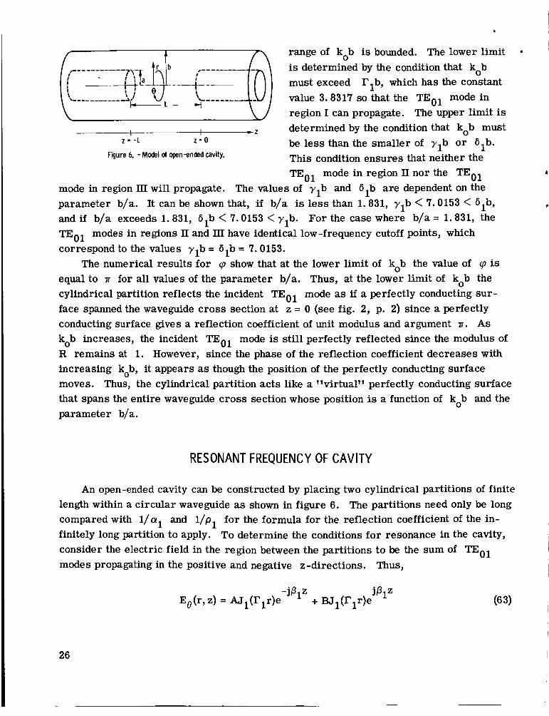
Figure 6. -Model of open-ended cavity.

. range of kob is bounded. The lower limit is determined by the condition that kob must exceed value 3.8317 so that the TEOl mode in region I can propagate. The upper limit is determined by the condition that kob must be less than the smaller of ylb o r 61b. This condition ensures that neither the TEOl mode in region II nor the TEOl

rib, which has the constant

mode in region III will propagate. The values of ylb and 61b are dependent on the parameter b/a. It can be shown that, if b/a is less than 1.831, ylb < 7.0153 < bib, and if b/a exceeds 1.831, tjlb < 7.0153 < ylb. For the case where b/a = 1.831, the TEOl modes in regions 11 and 111 have identical low-frequency cutoff points, which correspond to the values ylb = G1b = 7.0153.

The numerical results for cp show that at the lower limit of kob the value of cp is equal to B for all values of the parameter b/a. Thus, at the lower limit of kob the cylindrical partition reflects the incident TEOl mode as if a perfectly conducting sur - face spanned the waveguide cross section at z = 0 (see fig. 2, p. 2) since a perfectly conducting surface gives a reflection coefficient of unit modulus and argument 8 . As kob increases, the incident TEOl mode is still perfectly reflected since the modulus of R remains at 1. However, since the phase of the reflection coefficient decreases with increasing kob, it appears as though the position of the perfectly conducting surface moves. Thus, the cylindrical partition acts like a "virtual'' perfectly conducting surface that spans the entire waveguide cross section whose position is a function of kob and the parameter b/a.

#

RESONANT FREQUENCY OF CAVITY

An open-ended cavity can be constructed by placing two cylindrical partitions of finite length within a circular waveguide as shown in figure 6. The partitions need only be long

finitely long partition to apply. To determine the conditions for resonance in the cavity, consider the electric field in the region between the partitions to be the sum of TEOl I modes propagating in the positive and negative z-directions. Thus, I

compared with l/al and l/pl for the formula for the reflection coefficient Of the in- I

26

4.0 4.5 5.0 5.5 6.0 6.5 Dimension less resonant frequency, kob

Figure 8 - Ratio of cavity length to radius against dimensionless resonant frequency for radius ratio of 2082.

3.5 4.0 4.5 5.0 5.5 6.0 6.5 7.0 7.5 Dimensionless resonant frequency, kob

Figure 7. - Ratio of cavity length to radius against dimensionless resonant frequency for constant values of radius ratio.

At z = 0, the ratio of the reflected wave BJl(rlr) to the incident wave AJl(r1r) must equal the reflection coefficient R. Likewise, at z = -L, the ratio of the reflected wave

AJ 1 (r to the incident wave BJl(r1r)e must also equal R. Since R is equal to ejq these conditions are simply

jSIL -jSIL

and

It can be easily shown that, if there is to be a nontrivial solution for the amplitudes A and B, q and L must be related by the equation

27

I

jPIL 2 j % - j P 1 ~ - e = o e

A theory has been developed for a class of open-ended circular cylindrical microwave cavities by using Laplace transform and Wiener -Hopf techniques. Numerical re - sults were presented for the resonant frequency of the TEOll mode. The theory was

I shown to be in good agreement with experimental data.

which has the solution

The required spacing between the partitions to resonate the TEOll mode can be found by solving equation (66) for L by using the values of cp given in figure 5. The spacing for the TEOln resonant mode can be obtained simply by adding (n - 1)2n to cp before solving for L.

The numerical results for the TEOll mode are shown in figures 7 and 8 in the form of curves of L/b agdinst kob for typical values of the parameter b/a. The range of frequencies over which the cavity can be tuned by varying L/b is a strong function of b/a. The value b/a = 1.831 gives the maximum tuning range.

monly used in practice since it corresponds to locating the cylindrical partition at the radius where the electric field of the TEOl mode has its maximum intensity (i. e . , Jl(rlr) has a maximum at r = b/2.082). This value of b/a was used in the design of the cavity shown in figure 1 (p. 2) where the radius a was taken as the mean radius of the cylindrical partition. A data point corresponding to the measured values of L/b and kob for this cavity, as shown in figure 8, indicates that the theoretical and experimental results are in good agreement.

The numerical results shown in figure 8 a r e for b/a = 2.082. This value is com-

CONCLU SlON S

Lewis Research Center, National Aeronautics and Space Administration,

Cleveland, Ohio, April, 6, 1966.

28

REFERENCES

1. Crain, C. M. : The Dielectric Constant of Several Gases at a Wave-Length of 3.2 Centimeters. Phys. Rev., vol. 74, no. 6, Sept. 15, 1948, pp. 691-693.

2. Birnbaum, George: A Recording Microwave Refractometer. Rev. Sci. Inst., vol. 21, no. 2, Feb. 1950, pp. 169-176.

3. Crain, C. M. : Apparatus for Recording Fluctuations in the Refractive Index of the Atmosphere at 3.2 Centimeters Wave-Length. Rev. Sci. Inst. , vol. 21, no. 5, May 1950, pp. 456-457.

4. Crain, C. M.; and Deam, A. P.: An Airborne Microwave Refractometer. Rev. Sci. Inst., vol. 23, no. 4, Apr. 1952, pp. 149-151.

5. Adey, Albert W. : Microwave Refractometer Cavity Design. Canadian J. Tech., vol. 34, no. 8, Mar. 1957, pp. 519-521.

6. Thompson, M. C., Jr.; Freethey, F. E.; and Waters, D. M. : End Plate Modifica- tion of X-Band TEoll Cavity Resonators. IRE: Trans., vol. MTT-7, no. 3, July 1959, pp. 388-389.

7. Thorn, D. C. ; and Straiton, A. W. : Design of Open-Ended Microwave Resonant Cavities. IRE Trans., vol. MTT-7, no. 3, July 1959, pp. 389-390.

8. Marcuvitz, Nathan, ed. : Waveguide Handbook. McGraw-Hill Book Co. , Inc. , 1951. 9. Jahnke, Eugen; and Emde, Fritz: Tables of Functions with Formulae and Curves.

Fourth ed., Dover Pub., Inc., 1945.

10. Morse, Philip M. ; and Feshbach, Herman: Methods of Theoretical Physics. McGraw-Hill Book Co. , Inc., 1953.

11. Heins, A. E. ; and Silver, S. : The Edge Conditions and Field Representation Theorems in the Theory of Electromagnetic Diffraction. Proc. Cam. Phil. SOC., V O ~ . 51, pt. 1, Jan. 1955, pp. 149-161.

NASA-Langley, 1966 E-3351 29

.-

ERRATA

NASA Technical Note D-3514


By Norman C. Wenger

July 1966

Page 18, equations (44), (45), and (47): The right side should be multiplied by 1/2.

Page 18: Line 5 should read "since the function Jl(Aa)/Xa is equal to 1/2 at X = 0, has a zero derivative with respect. t1

Page 18, equation (46): The coefficient of the right side should be -1/17 instead of 2/17.

Page 18: Line 12 should read "since this function is equal to -l/s(b/a - a/b) at X = 0, has a zero derivative with respect. *'

Page 18, equation (47): The quantity ( 1 - - - should be [ - $). rn rn

Page 19, equations (48) and (49a): The right side should be multiplied by -1/2.

Page 19: Line 9 should read ltThe quantity -1/2(1 - a 2 2 /b ) has been arbitrarily associ-

ated with the factor @. The."

Page 20: Line 9 should read "Since an and yn approach (n + 1/4)17/a as n -00, it is apparent that the infinite product. l t

Page 20, line 10: The quantity 1 + - should be 1 + ( z ) ( n + 1/4)17

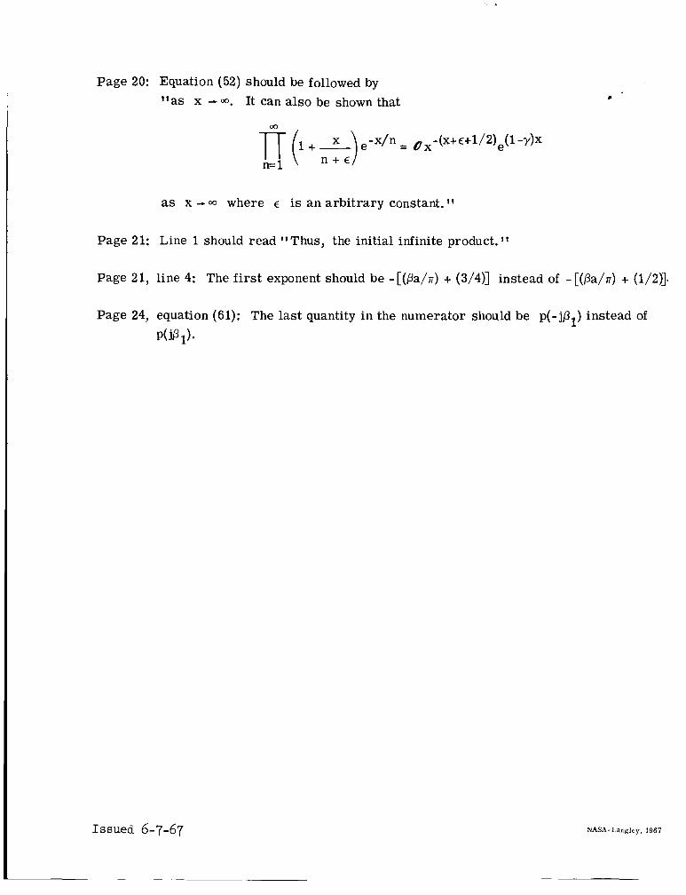
Equation (52) should be followed by "as x - co. It can also be shown that

as x -CO where E is an arbitrary constant.v*

Page 21: Line 1 should read "Thus, the initial infinite product. * *

Page 21, line 4: The first exponent should be -[(Pa/n) + (3/4)] instead of -[(pa/n) + (1/2)l.

Page 24, equation (61): The last quantity in the numerator should be p(-jP,) instead of p(jP1).

Issued 6-7-67 NASA-Langley, 1967

- ~ ~

ERRATA



By Norman C. Wenger

July 1966


Page 18: Line 5 should read "since the function Jl(ha)/Xa is equal to 1/2 at X = 0, has a zero derivative with respect. 1t

Page 18, equation (46): The coefficient of the right side should be -1/n instead of 2/77.

Page 18: Line 12 should read "since this function is equal to -l/n(b/a - a/b) at h = 0, has a zero derivative with respect. t *

Page 18, equation (47): The quantity 1 - Y should be 1 - - . ( 3 ( :I) Page 19, equations (48) and (49a): The right side should be multiplied by -1/2.

2 2 Page 19: Line 9 should read "The quantity -1/2(1 - a /b ) has been arbitrarily associated with the factor @. The. t t

Page 20: Line 9 should read "Since an and yn approach (n + 1/4)s/a as n --, it is apparent that the infinite product. l t

Page 20, line 10: The quantity 1 + - should be ( C) [ + (n ::/4)77]

Equation (52) should be followed by "as x - 00. It can also be shown that

as x - 00 where E is an arbitrary constant. ''

Page 21: Line 1 should read "Thus, the initial infinite product."

Page 21, line 4: The first exponent should be -[(pa/n) + (3/4)] instead of -[(pa/lr) + (1/2)1.

Page 24, equation (61): The last quantity in the numerator should be p(-jP,) instead of p(jPl).

NASA-Langley, 1967

ERRATA .



By Norman C. Wenger

July 1966


Page 18: Line 5 should read "since the function Jl(ha)/ha is equal to 1/2 at h = 0, has a zero derivative with respect. l 1

Page 18, equation (46): The coefficient of the right side should be -l/r instead of 2/r.

Page 18: Line 12 should read "since this function is equal to -l/r(b/a - a/b) at h = 0, has a zero derivative with respect. '*

Page 18, equation (47): The quantity ( 1 ~ - - I:) should be [ - rn


2 2 Page 19: Line 9 should read **The quantity -1/2(1 - a /b ) has been arbitrarily associated with the factor @. The. ? l

Page 20: Line 9 should read "Since cyn and 7, approach (n + 1/4)r/a as n -m, it is apparent that the infinite product. '*

Page 20, line 10: The quantity 1 + - should be ( t) [I+ (n :;,4)r]-

Equation (52) should be followed by "as x -00. It can also be shown that

00

as x - ~0 where E is an arbitrary constant. l1

Page 21: Line 1 should read "Thus, the initial infinite product. l1

Page 21, line 4: The first exponent should be -[(Pa/a) + (3/4)] instead of -[(Pa/n) + (1/2)].

Page 24, equation (61): The last quantity in the numerator should be p( - jp,) instead of p(jPl).

Issued 6-7-67 NASA-Langley, 1967

~~

ERRATA 6



By Norman C. Wenger

July 1966

Page 18,

Page 18:

Page 18,

Page 18:

Page 18,

Page 19,

Page 19:

Page 20:

Page 20,

equations (44), (45), and (47): The right side should be multiplied by 1/2.

Line 5 should read "since the function Jl(Aa)/Aa is equal to 1/2 at A = 0, has a zero derivative with respect."

equation (46): The coefficient of the right side should be -l/r instead of 2 / ~ .

Line 12 should read *?since this function is equal to -l/r(b/a - a/b) at A = 0, has a zero derivative with respect." -

equation (47): The quantity

equations (48) and (49a): The right side should be multiplied by -1/2.

Line 9 should read "The quantity -1/2(1 - a 2 2 /b ) has been arbitrarily associ-

ated with the factor @. The. ''

Line 9 should read "Since cyn and y, approach (n + 1/4)r/a as n -00, it is apparent that the infinite product. f t

line 10: The quantity

Equation (52) should be followed by "as x - 00. It can also be shown that

00

as x - 00 where E is an arbitrary constant. ''


Page 21, line 4: The first exponent should be -[(Pa/n) + (3/4)] instead of -[(Pa/n) + (1/2)l.

Page 24, equation (61): The last quantity in the numerator should be p(-jP,) instead of p(jP1).

Issued 6-7-67

-

NASA-Langley, 1967

L

ERRATA



By Norman C. Wenger

July 1966


Page 18: Line 5 should read "since the function Jl(Xa)/Xa is equal to 1/2 at h = 0, has a zero derivative with respect."

Page 18, equation (46): The coefficient of the right side should be -l/a instead of 2/a.

Page 18: Line 12 should read "since this function is equal to -l/n(b/a - a/b) at X = 0, has a zero derivative with respect. '*


2 2 Page 19: Line 9 should read "The quantity -1/2(1 - a /b ) has been arbitrarily associated with the factor @. The."

Page 20: Line 9 should read "Since an and yn approach (n + 1/4)a/a as n - 00, it is apparent that the infinite product. *'

Page 20, line 10: The quantity 1 + - should be ( 5) p+ (n :L]. I

Equation (52) should be followed by **as x - m. It can also be shown that L

m

as x - m where E is an arbitrary constant.


Page 21, line 4: The first exponent should be -[(pa/n) + (3/4)] instead of -[(pa/r) + (1/2)3.

Page 24, equation (61): The last quantity in the numerator should be p(-jP,) instead of p(jPl).

Issued 6-7-67 NASA- Langley, 1967

~ ~ ~

‘ T b e aerottairical and space activities of tbe United S a t e s sball be condscted so ~ L T to contribste - . . to the expamion of human 15130iuI-

edge of phenomellg in the crtmospbsre aa8 spae. The Adntinirtratiun sbdi provide for tbe widest prgciicabie and appropriate dissemination of information roncenrkrg itr r/ctiviia aad the resdtr ikeof.’ ’

-NAnorai AEROHAUTKS AKD SPACE ACT OF 1958

NASA SCIENTIFIC AND TECHNICAL PUBLICATIONS

TECHNICAL REPORTS important, complete, and a lasting contribution to existing knowledge.

TECHNICAL NOTES: of importance as a mtribution to existing knowledge.

TECHNICAL MEMOIUNDWMS: I n f o r d o n receiving limited disai- burioa imause of preiiminary data, security classification, or other reasons.

CONTRACTOR REPORT5 Technical information generated in con- nection wkb a NASA conrratf or grant and released under NASA auspices.

Scientific and technical information considered

Information less broad in scope but nevertheless

TECHNICAL TRANSLATIONS Information published in a foreign language considered to merit NASA distribution in English.

TECHNICAL REPRINTS Information derived from NASA activities and initially published in the form of journal articles.

SPECIAL PUBLICATIONS: Information derived from or of d u e to NASA activities but not necessarily reporting the r e d t s Of individual NASA-programmed scient& &om. Publications include coderena proceedings, monographs, data compilations, handbooks, S O P I C C ~ ~ ~ S ,

and special biMigraphies.

&faits on the availability of tkst pu&#idons mery be o b i m i d bs

SClEMFK AND ECWWU HFORMATfON MVEKM

NATIONAL AERONAUTICS AND SPACE ADMl Worhirdocr,D.C M46

theory open-ended circular cylindrical microwave cavity · the open-ended microwave cavity ... (ic)...

Documents