The Pakistan Development Review 43 : 1 (Spring 2004) pp. 73–93

Elasticity and Buoyancy of the Tax System in Pakistan

FAIZ BILQUEES*

This paper examines the elasticity and buoyancy of the tax system for the period

1974-75–2003-04. The elasticity of the total tax revenue both with respect to the total GDP and the non-agricultural GDP base is less than unity. Overall, sales tax takes the lead by way of improving revenues. The high coefficient of income tax inclusive of withholding tax, which is an indirect tax, is high. Excluding the withholding tax leads to a lower coefficient. Sales tax with respect to imports and manufacturing also takes care of loss of revenue due to lowering of tariff and excise duties. However, the sales tax coefficient with respect to the GDP base reflects the inclusion of service sector and utilities in the sales tax net, which has serious implications for the poor. The estimates of buoyancy suggest that tax changes did not lead to significant revenue augmentation. The low buoyancy of income tax exclusive of the withholding taxes implies that imposition of massive withholding taxes coupled with an increase in the taxable income limits is working at cross purposes.

INTRODUCTION

Tax responsiveness to changes in income is a crucial variable in projecting the tax revenues, and is a basic criterion for a good tax system. This response is measured by two concepts: tax elasticity which measures the automatic response of revenue to income changes, net of discretionary changes; and tax buoyancy which measures the total response of tax revenue to changes in income. In developing countries generally, the major taxes tend to have low elasticity and sometimes even the buoyancy is low. This is mainly due to the inherent weaknesses in economic structure where a large majority remains out of the tax net due to low average income levels, and unorganised nature of most economic activities, which erode the income tax base. However, an equally important factor has been the provision of massive tax incentives and exemptions to the manufacturing sector over extended

Faiz Bilquees is Joint Director at the Pakistan Institute of Development Economics, Islamabad. Author’s Note: I am grateful to two anonymous referees of the PDR for their very useful

comments and suggestions on the paper. I would also like to thank Dr A. R. Kemal, Director, PIDE, for his valuable guidance at every stage in the preparation of this paper. Thanks are also due to Mr Imtiaz Ahmad, PhD Fellow at PIDE, for his computational assistance.

Faiz Bilquees

74

periods in most of these countries. As a result, the levels of budget deficits and borrowings, and/or aid requirements become unsustainable over time. Domestic resource mobilisation and reduction of budget deficits then become the major targets of the Structural Adjustment Programmes in the short run, and in many cases even in the long run.

In the case of Pakistan, while the initial stages of rapid economic growth were characterised by massive tax concessions, the nationalisation in the 1970s resulted in a massive shift to the informal sector, which became synonymous with the parallel or underground economy in a very short period.1 The continued reduction in formal employment, as a policy measure since the 1990s, has further expedited the expansion of the informal sector. As compared to 20 percent in 1974, after the nationalisation in 1972, and to 25 percent in 1990-91, it accounted for 54 percent of the GDP in 1998 [see Kemal (2003)]. As a result of the distortions created in the economy over time, Pakistan has had a chain of stand-by and structural adjustment and stabilisation programmes from 1973-74 until 2003. All the programmes had a special focus on tax reforms including improved tax governance, increasing the share of direct taxes, expanding the tax net, imposition of sales tax on a wider scale, and improving the tax elasticity and buoyancy. However, the implementation of the reforms particularly in the fiscal sector was visible only for the last programme of 2000-03. The expanded enforcement of the sales tax, rationalising the exercise of power by the tax officials, and some expansion in the tax net has been achieved. However, the overall tax revenues as a percentage of GDP still average less than 15 percent and the share of indirect taxes still exceeds 60 percent of total tax revenues.

When the elasticity of major revenue sources remains low despite tax reforms either due to low base, or due to evasion or avoidance, the governments raise additional resources through discretionary measures. Then, the growth of tax revenues comes through high buoyancy rather than through elasticity. The objective of this paper is to measure the buoyancy and elasticity of the tax system in Pakistan over the period 1974-75 to 2002-03 by using the Divisia Index Approach, and analyse the factors responsible for the resulting size of elasticity coefficients. The coefficient of elasticity depends on the level of tax rates, the progressivity of the rate structure, and the responsiveness of the tax base to changes in income. This makes it possible to break up the value of elasticity into two components—the response of the tax base to a change in income, and the response of the tax yield to a change in the tax base of individual taxes through decomposition of elasticities [see Musgrave (1959)].

1Government policies to exempt the four units of weaving from taxes, and in general the policies that favoured micro enterprises over the large-scale enterprises led to a massive shift to the informal sector.

Elasticity and Buoyancy of the Tax System

75

The value of base to income elasticity does not depend on the progressivity of tax rates; it simply relates the responsiveness of the tax base to a change in income. The growth of the base depends on the way the structure of the economy changes with economic growth. The tax-to-base elasticity depends on the tax rates; if the rate structure is progressive or if there is an improvement in tax administration, the tax-to-base elasticity will be raised by preventing evasion. The decomposition of elasticity in this manner permits us to identify the source of growth of tax revenues.

The paper is structured as follows. Section II very briefly reviews the trends in direct and indirect taxes, and highlights the policies adopted to improve the tax system. Section III describes the data sources and the methodology used for the estimation of elasticity in this paper. Section IV analyses the results based on the Divisia Index Estimates of elasticity and buoyancy, and the decomposition of elasticities to describe the prevailing situation in the tax system and its implications for the economy of Pakistan. Finally, Section V concludes the paper with some policy recommendations.

I. TRENDS IN DIRECT AND INDIRECT TAXES2

Pakistan’s tax system in its ability to raise adequate tax revenues has not been any better than many other developing countries. It has not been able to generate more than 14 percent of tax revenues in relation to GDP. This lacklustre performance is largely attributed to three inherent weaknesses of Pakistan’s tax system, i.e., narrow and distorted tax base, over-reliance on indirect taxes, and weak tax administration. For example, in the case of personal income tax, the fringe benefits of the employees remained exempt for a very long period of time. Similarly, the exemptions from taxation of gross income have been quite generous, amounting to one hundred thousand rupees in the budget for 2003-04. The agriculture tax, mainly a provincial tax, has not been fully implemented due to the loopholes provided in the legislation for agriculture tax. On the other hand, the industrial sector and the external sector have enjoyed massive concessions and tax holidays in the 1960s and 1970s. A large number of commodities were exempted from customs and excise duties without adequate monitoring to prevent the abuse of this concession. The most important element in this “exemption exercise” has been the “ad hocism” of the policy measures. All these special departures result in the loss of revenue and reduce the elasticity of tax revenues in relation to GDP. Furthermore, taxes have failed to increase as a share of GDP as the widespread tax avoidance/evasion—and the inability of the tax authorities to enforce tax laws—has undermined the confidence of the taxpayers in the efficacy of the tax system.

2 All the tax revenues are the consolidated Federal and Provincial taxes. Local taxes, however, are not included.

Faiz Bilquees

76

The resulting inadequacy of revenues is reflected in Table 1, and total tax revenues average 13 percent of GDP over the period 1974-75 to 2002-03.3,4

Table 1

Composition of Consolidated Federal and Provincial Taxes in Pakistan Percentage

of GDP Percent Share in

Total Taxes Percent Share of Individual Taxes

in Indirect Taxes

Period Tax

Revenue Direct Taxes

Indirect Taxes

Direct Indirect Customs Sales Central Excise

1974-75 8.03 1.12 6.91 13.2 86.8 50.0 11.3 38.7 1976-77 11.94 1.78 10.16 17.4 82.6 47.5 10.5 42.0 1978-79 12.94 1.71 11.23 14.6 85.4 50.7 9.7 34.6 1980-81 14.12 2.52 11.60 20.7 79.3 51.7 10.5 37.8 1983-84 13.18 2.19 10.99 17.4 82.6 51.5 11.1 37.4 1986-87 14.48 1.94 12.54 16.4 83.6 58.9 9.9 31.2 1987-88 13.84 1.84 12.40 13.0 87.0 47.0 10.8 19.1 1990-91 12.70 2.03 12.00 18.0 82.0 54.9 17.6 27.5 1993-94 13.22 2.80 10.67 25.1 74.9 49.7 23.5 26.9 1995-96 14.35 3.72 10.41 29.1 70.9 46.8 26.3 26.9 1997-98 13.26 3.91 10.64 35.0 65.0 39.1 28.3 32.6 1999-00 12.90 3.67 9.33 32.5 67.5 26.4 49.9 23.7 2000-01 12.90 3.75 9.14 31.8 68.2 24.3 57.4 18.3 2001-02 13.22 4.06 9.14 35.3 64.7 18.3 63.7 18.0 2002-03 13.80 2.89 9.91 32.2 67.8 18.9 65.9 15.2 Source: Pakistan Economic Survey (Various Issues).

Direct taxes comprise incomes of the non-corporate and the corporate sector including the withholding taxes.5 The share of direct taxes remained very low until late 1980s, averaging 2 percent of the GDP, largely due to the extended tax holidays and exemptions in the 1960s and early 1970s, but picked up in the early 1990s. These increased by more than 3 percent of the GDP in the early 1990s and averaged 3.5 percent of GDP between 1995 and 2003. The share of indirect taxes averaged between 11-12 percent from late 1970s to mid-1990s, and registered a decline thereafter to around 9 percent of GDP.

However, over time, the shift in the shares of direct and indirect taxes as a percent of total taxes has been quite significant. The share of direct taxes increased from 13 percent in 1974-75 to 35 percent in 2001-02, but declined to 32.3 percent in 2002-03, while that of the indirect taxes declined from 86.8 percent to 68 percent over the same period.

3Even though there has been a re-basing of national accounts, a large number of enterprises may have been outside the GDP estimates. And in any case, informal enterprises included in the GDP have not been paying taxes due to concessions as well as tax evasion.

4The disaggregated financial statistics for present Pakistan, after the creation of Bangladesh, begin in 1974-75, as announced by the State Bank of Pakistan.

5Other direct taxes including wealth tax, gift tax, and estate duty have been abolished, and the share of workers’ welfare fund is very small in the direct taxes.

Elasticity and Buoyancy of the Tax System

77

It is important to note that the increase in the share of direct taxes in the 1990s has come from the massive increase in the withholding taxes. In the late 1960s, withholding taxes were levied only on three sources of income: salaries, interest on securities, and payments to non-residents. Until 1979, six kinds of payments were subject to withholding tax, which increased to 19 in 1994-95 and to 25 in 1999-00 [CBR (March 2003)].

Among the indirect taxes, significant changes have been observed over time. Customs duties which formed the major chunk of tax revenues until early 1980s, have been rationalised from a maximum rate of around 125 percent in 1987-88 to 25 percent in 2002-03. Consequently, the share of customs duties in total indirect taxes has declined from 54 percent in 1990-91 to 19 percent in 2002-03. It has been decided that they will now be used only for protection purposes. However, the decline in the customs duties and the excise duties has been picked up by the sharp increase in the sales tax revenue on imports and domestic production.

Until late 1980s, sales tax on domestic production and imports was administered in such a way that it was no different from excise duties on domestic production and customs duties on imports. As such, it served no useful propose but affected the distribution of tax revenues between the provinces and the federal government. The generalised sales tax was introduced very comprehensively in 1989-90 and its rates have been revised quite frequently to increase tax compliance by the unregistered taxpayers and to generate additional tax revenues. Between 1990-91 and 1998-99 general sales tax revenues increased from 1.65 percent of GDP in 1990-91 to 2.77 percent in 1994-95, but these declined to 2.33 percent in 1998-99. However, as a result of the increase in the sales tax base, by extending the sales tax net in 1999-00, sales tax revenues increased to 3.7 percent of GDP in that particular year. After averaging 4.6 percent in the following two years, sales tax revenues increased to 5.9 percent of GDP in 2002-03. The slow growth in sales tax revenues was due to the revisions in tax rates for some commodities. In the budget for 2003-04, sales tax has been fixed at 12.5 percent for all entities.

Frequent revisions in the tax rates have been adopted as a measure of fiscal policy to increase revenues. The personal income tax rates for salaried and non-salaried persons have been unified; the minimum threshold for income tax was raised from Rs 40,000 in 1988-89 to Rs 60,000 in 1998-99, and five tax rates ranging from 7.5 percent to 35 percent were introduced. In the budget for 2002-03 and 2003-04, the minimum thresholds were raised to 80,000 and 100,000 rupees with the objective to enhance revenue collection by lowering the taxable income levels. Similarly, in the corporate sector, the banking company’s rates have been continuously slashed from 60 percent in 1992-93 to 50 percent in 2002-03. This decline at the rate of 3 percent per annum will continue until the reform target of 35 percent is achieved within a five-year period.

Faiz Bilquees

78

In the late 1990s, a number of important tax reforms were announced, including the introduction of the book-keeping requirements into the Income tax Ordinance in February 2000, whereby 25 percent of the 1.2 to 1.5 million returns under the self-assessment schemes were to be subjected to random audit. The announcement of 25 percent random audit under self-assessment was meant to encourage the public at large to file their returns without fear of undue harassment by the tax officials. In the fiscal year 2002-03 only two percent of the returns were audited, and while the CBR said it was not a random audit, it did not specify any other basis for it. This was essential to mitigate the general complaint against the tax authorities—that they unnecessarily harassed the taxpayers in the private sector in the name of detailed scrutiny. In this regard, the powers of the tax inspectors were also severely curtailed; they are not allowed to open the returns filed. However, the elimination of various tax exemptions, such as the withdrawal of tax-whitener schemes that guaranteed immunity from tax probes, making the interest income of national saving certificates taxable, bringing in-kind benefits of the employees within the ambit of income tax, and measure taken to make agricultural income tax fully operational have helped improve tax collection and the tax structure to some extent. These measures, it is expected, would lead to an increase in the number of taxpayers in the coming years, provided, the continuity of the policies is maintained.

III. DATA AND METHODOLOGY

The relevant data for this study for the period 1974-75 to 2002-03 are taken from the Central Board of Revenue Yearbook and the Pakistan Economic Survey. Contrary to the earlier studies [Chowdhury (1962); Khan (1973); Jeetun (1978); Gillani (1986); Kemal (1995)] the data used in this study were tested for stationarity with the objective to use co-integration technique rather than the simple OLS. The details of the requisite data transformation/adjustments and the outcomes are reported in Appendix I. It will be seen from the appendix table that the series are non-stationary because the variables are integrated with different orders, so the data fail to meet the pre-requisites of the Co-integration technique for estimation. Therefore, we use the Vector Auto-regressive (VAR) technique to estimate elasticity and buoyancy for this study.

To estimate the built-in elasticity of a tax system, the historical revenue data need to be adjusted for the effects on revenue from discretionary tax changes as applied from time to time. The three common methods adopted to eliminate the effects of discretionary changes in taxes include the proportional adjustment method; the constant rate structure; and the dummy variable method. However, a complete adjustment of historical revenue series is not possible in any of the methods.. The first method requires use of budget estimates of tax yields resulting from discretionary changes. Not only are such data difficult to obtain, their reliability is questionable as the actual discretionary outcomes may differ significantly from the

Elasticity and Buoyancy of the Tax System

79

changes proposed in the budget. The data on discretionary revenues provided by the Central Board of Revenue are not only incomplete, these underscore two limitations of the data. Firstly, some of the measures proposed at the time of budget-making were never implemented, and therefore the financial effect could be different than reported in the data provided. Secondly, the calculation of financial effect of tax measures is based on the ‘static’ model. No dynamics have been captured, therefore ex-ante and ex-post differential can exist.

The second method—the constant rate structure method—is not used very commonly because it places heavy demands on the availability of data. It requires data on effective tax rates and on the changing composition of the bases. Provided these data are available and both the tax and its base are defined narrowly enough to permit application of the reference year rates to later year tax bases, this method generates the most accurate revenue series. However, such data are hard to come by particularly in the less developed countries.

The dummy variable method does not require the use of disaggregated data on taxes, but it cannot be used properly when discretionary tax changes are quite frequent in the past. Furthermore, even if the discretionary changes are not very large, the specification of the estimation equations can be problematic unless there is information on the nature of the tax changes and the extent to which their effects are independent of one another. In the case of Pakistan, there have been changes in taxes almost every year, and the Central Board of Revenue has generally been over-estimating tax revenues.

Therefore, we choose to estimate elasticity by the Divisia Index (DI) Method—since it does not involve the traditional adjustment of the historical revenues to eliminate the effects of discretionary tax measures. The measurement of elasticity by the DI approach involves three steps: first, the effects of discretionary tax measures on revenues are estimated by an index that isolates the automatic growth of revenues from the total growth; second, the buoyancy of tax revenue is estimated with respect to GDP by a standard regression technique; and third, the estimated buoyancy is adjusted by a suitable transformation of the index of discretionary revenue, estimated in step one, to obtain the estimate of elasticity of the tax yield. 6

The DI method uses only historic data and does not require the collection of specific information on revenue effects of discretionary tax changes, or on the frequency of past discretionary tax changes. However, two caveats may be noted: first, it may underestimate/over-estimate the revenue effects of discretionary tax change; and secondly, in case of large revenue effects, it may give unsatisfactory results.

6As explained in Section III. (a) from Equation 8a to Equation 13.

Faiz Bilquees

80

III.(a) Divisia Index Method 7

The Divisia Index, derived from a weighted sum of growth rate of factor inputs, is an index of factor inputs, for the measurement of technical change. The index of technical change is the ratio of an index of total productivity to an index of factor productivity, the latter measured by the Divisia index. This measure implies that the percentage increase in total productivity caused by technical progress is equal to the percentage increase in output divided by the percentage increase in factor inputs. The appropriateness of this measure is based on its property of invariance, i.e., if there is no technical change, the growth in total productivity is entirely due to factor inputs. A change in the Divisia index, therefore, gives a measure of the change in total productivity that shifts the production function due to all sorts of factors that are jointly termed as ‘technical change’.

Intuitively, the effects of technical change are analogous to the effects of discretionary tax measures. Discretionary tax measures produce changes in tax yields over and above those caused by automatic growth in tax bases as technical changes induce changes in total productivity over and above that induced by factor inputs. This analogy can be explained more specifically as follows: assume that there exists a tax function that shows the tax yields resulting from k bases. This is analogous to the production function that shows the aggregate output given by n factor outputs. For the given tax structure and the given configuration of the tax bases, tax yield will not change in the absence of any discretionary tax measures, just as, for the given level of factor inputs, there is no change in output in the absence of technical change. On the other hand, for a given set of tax bases, if we assume a discretionary tax measure is adopted that alters tax rates and/or exemption levels of one or more categories of taxes, the revenues produced are different from what they would be in the absence of such an action. This difference or change in the tax yield arises due to the induced shift (of either the intercept, the slope, or both) in the aggregate tax function due to the discretionary tax action analogous to that caused by technical change in the production function, which produces a different output from that produced without technical change.

A Divisia index of discretionary tax change, therefore, can be considered as analogous to the index of technical change. This index should be equal to the percentage increase in total tax yield divided by the percentage increase in total tax yield owing to the automatic increase in the bases. Similarly, like the index of technical change, a change in this index should reflect the overall revenue effects of discretionary tax measures.

The applicability of this index of discretionary tax change is subject to two conditions: it must be derived from an aggregate tax function analogous to a production function; and it must posses the invariance property.

7 This section is based on Choudhry (1979).

Elasticity and Buoyancy of the Tax System

81

The necessary and sufficient conditions that ensure the invariance property of the Divisia index are as follows: there exists a well-defined continuously differentiable aggregate function, f (x1 (t), …, xk(t)); the function f is linear homogenous (implying constant returns to scale).

The existence of condition (a) is fundamental to the existence of a relationship between the tax yields and the tax bases, and the concepts of elasticity and buoyancy. In the absence of an underlying aggregate tax function, there is a fundamental indeterminancy about the tax yield and tax bases. The “continuously differentiable” character of the aggregate tax function ensures the regularity of such a function, and prevents the erratic behaviour of the tax yield. Indeed the existence of condition (a) is central to the derivation of the Divisia index.

The requirement of linear homogeneity is more restrictive because in a progressive rate structure, such as that in case of income tax, it is clear that an increase in per capita incomes will produce more than proportional increase in revenues. However, the elimination of this restriction by Hulten (1973)8 made possible the application of the DI to aggregate functions with non-constant returns without violating the invariance property. It is important, however, to point out here that the assumption of a homogeneous aggregate tax function is justified in case of LDCs where tax ratios (tax/GDP) have increased relatively faster than in the developed countries but the average increase has been rather small.9 These trends in aggregate revenues can be written as a homogeneous function of GDP (x)

µ= axT … … … … … … … (1)

When x rises over time, the tax ratio remains constant or rises as the value of µ (buoyancy) equals or exceeds unity.

This homogeneous tax function has been extensively used in empirical studies for estimating the buoyancy or the elasticity of tax revenues.

Derivation of the DI of Discretionary Tax Revenues

Using the continuously differentiable aggregate tax function at each point in time:

];)(...,)([)( ttxtxftT ki= … … … … … (2)

Where T is the aggregate tax yield; x denotes the proxy tax base for k categories of taxes; and t, the time variable is the proxy for discretionary tax measures. The effects of discretionary tax measures in Equation (3) are obtained by taking the logarithm of the tax function, differentiating with respect to time and re-arranging as:

8As reported in Choudhry (1979). 9While Choudhry (1979) quotes Chelliah, et al. (1975), reporting that the average tax ratios of

developing countries has increased by 13.6 percent for 1961-68, to 15.1 percent for 1969-70, it will be seen from Table 1 that for Pakistan this ratio averages only 14 percent for 1990-91 to 2002-03.

Faiz Bilquees

82

)()(

)()()(

)()()(

1 txtx

tftxtf

tTT

tftf

i

ik iit &&∑−= … … … … (3)

Setting )()(

)()(

tDtD

tftf t &= and )(

)()()(

ttf

txtfi

ii β= where D(t) is the DI of

discretionary tax change; Equation (3) is rewritten as

)()(

)()()(

)()(

1 txtx

ttTtT

tDtD

i

ik

i&&

&

&∑β−= … … … … … (4)

Where; )()(

tDtD& , represents the growth of tax revenues owing to discretionary tax

measures. To obtain the index of discretionary tax revenue over the time interval [0,n]

Equation (4) is integrated as:

⎟⎟⎟

⎠

⎞

⎜⎜⎜

⎝

⎛β−⎥

⎦

⎤⎢⎣

⎡= ∑∫ dt

txxt

TnT

DnD

i

ik n

i )()(exp

)0()(

)0()(

10

& … … … (5)

Normalising by setting D(0=1), D(n) represents the index of revenue growth only due to discretionary tax measures over time.

Star and Hall (1976) simplified the right-hand side of Equation (5) by replacing the fluctuating βi(t) by a constant )(~ tiβ which is some form of weighted

average of the βi(t). This transformation yields Equation (6) of the form:

dttxtxtdt

txtx

i

ini

i

in

)()()(

)()(~

00&&

∫∫ β=β … … … … (6)

integrating the left-hand side of Equation (6) leads to

∫ β=⎟⎟⎠

⎞⎜⎜⎝

⎛β n

i

ii

i

ii dt

txtxt

xnx

0 )()()(

)0()(log~ &

… … … … (7)

In Equation 7 the growth rate of tax revenues is divided by the index of automatic growth of tax revenues as measured by the denominator.

If the left-hand side of Equation (7) is put into the right-hand side of Equation (5), we get

Elasticity and Buoyancy of the Tax System

83

∏=

β⎥⎦

⎤⎢⎣

⎡=

k

i i

i ix

nxT

nTnD1

~

)0()(

)0()()( … … … … … (8)

In Equation (8) the growth of discretionary tax revenues is the difference between the growth rates of total tax revenues and automatic tax revenues, which is a sum of the growth rates of the (proxy) bases where the weight )(~ tiβ is obtained from Equation (7).

In log form Equation (8) can be written as:

⎟⎟⎠

⎞⎜⎜⎝

⎛β−⎟⎟

⎠

⎞⎜⎜⎝

⎛= ∑

)0(log~

)0()(log)(log )(

1 xix

TnTnD nik

i … … … (8a)

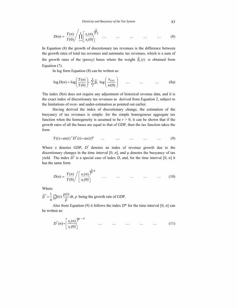
The index D(n) does not require any adjustment of historical revenue data, and it is the exact index of discretionary tax revenues as derived from Equation 2, subject to the limitations of over- and under-estimation as pointed out earlier.

Having derived the index of discretionary change, the estimation of the buoyancy of tax revenues is simple: for the simple homogenous aggregate tax function when the homogeneity is assumed to be r > 0, it can be shown that if the growth rates of all the bases are equal to that of GDP, then the tax function takes the form

µ== )()()()( * taxtDtaxtT r … … … … … (9)

Where x denotes GDP, D* denotes an index of revenue growth due to the discretionary changes in the time interval [0, n], and µ denotes the buoyancy of tax yield. The index D* is a special case of index D, and, for the time interval [0, n] it has the same form

*~

)0()(

)0()()(

β⎥⎦

⎤⎢⎣

⎡=

i

ix

nxT

nTnD … … … … … (10)

Where

ρρρ

β=β ∫ ,)()(1~0

* dtttn

n being the growth rate of GDP.

Also from Equation (9) it follows the index D* for the time interval [0, n] can be written as:

r

xnxnD

i

i−µ

⎥⎦

⎤⎢⎣

⎡=

)0()()(* … … … … … (11)

Faiz Bilquees

84

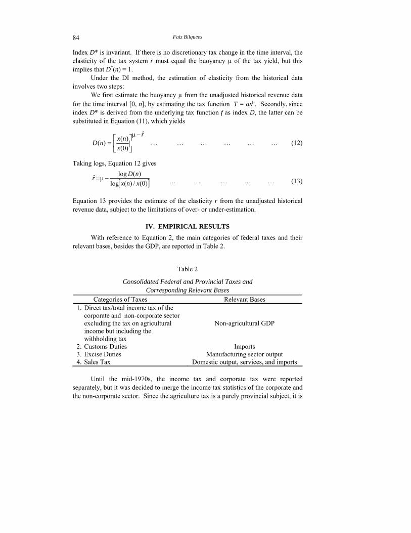
Index D* is invariant. If there is no discretionary tax change in the time interval, the elasticity of the tax system r must equal the buoyancy µ of the tax yield, but this implies that D*(n) = 1.

Under the DI method, the estimation of elasticity from the historical data involves two steps:

We first estimate the buoyancy µ from the unadjusted historical revenue data for the time interval [0, n], by estimating the tax function T = axµ. Secondly, since index D* is derived from the underlying tax function f as index D, the latter can be substituted in Equation (11), which yields

r

xnxnD

ˆ

)0()()(

−µ⎥⎦

⎤⎢⎣

⎡= … … … … … … (12)

Taking logs, Equation 12 gives

[ ])0(/)(log)(logˆ

xnxnDr −µ= … … … … … (13)

Equation 13 provides the estimate of the elasticity r from the unadjusted historical revenue data, subject to the limitations of over- or under-estimation.

IV. EMPIRICAL RESULTS

With reference to Equation 2, the main categories of federal taxes and their relevant bases, besides the GDP, are reported in Table 2.

Table 2

Consolidated Federal and Provincial Taxes and Corresponding Relevant Bases

Categories of Taxes Relevant Bases 1. Direct tax/total income tax of the

corporate and non-corporate sector excluding the tax on agricultural income but including the withholding tax

2. Customs Duties 3. Excise Duties 4. Sales Tax

Non-agricultural GDP

Imports Manufacturing sector output

Domestic output, services, and imports

Until the mid-1970s, the income tax and corporate tax were reported separately, but it was decided to merge the income tax statistics of the corporate and the non-corporate sector. Since the agriculture tax is a purely provincial subject, it is

Elasticity and Buoyancy of the Tax System

85

not included; but the withholding tax of the corporate sector is included in the income tax. The relevant base for customs duty is the value of imports. Prior to the policy of tariff reduction, customs duty was the major source of tax revenues, but now it is only used for protection purposes. Similarly, prior to mid-1990s, excise duty was levied on the manufacturing sector, retail businesses, financial services, and other services. However, with the enlargement of the sales tax net, and its effective implementation, excise duties are now levied mainly on domestic manufacturing. Sales tax is levied on domestic output including services and imports.

Following the DI approach, the buoyancy is estimated by estimating the tax function T = ax µ , with respect to total GDP, and the elasticity estimates are obtained by adjusting buoyancy as given by Equation 13. Since the overall effect of discretionary change is shown to increase revenues, the elasticity of tax revenues is expected to be smaller than the buoyancy. However, in Table 3 we see that the coefficients of elasticity slightly exceed those of the buoyancy for both the customs duties and the sales tax in the long run. In case of customs duties, however, the elasticity coefficient is considerably lower than unity. The high elasticity of sales tax with respect to the total GDP base may clearly be attributed to the extension of sales tax to electricity, gas, and petroleum products. These items constitute the basic input to all the production and distribution network in the economy. The inelastic demand for these inputs makes the revenues from the sales tax more elastic with reference to GDP base.

Table 3

Elasticity and Buoyancy of Consolidated Federal and Provincial Taxes (with GDP Base)

Total Tax

Income Tax

Customs Duty

Excise Duty

Sales Tax

Short run 1974–2003 Buoyancy 0.44 0.40 –0.06 0.48 0.42 Elasticity 0.33 0.31 –0.20 0.06 0.38 Long run 1974–2003 Buoyancy 0.92 1.23 –1.19 0.48 1.41 Elasticity 0.88 1.21 0.43 0.44 1.50

The short-run elasticities are included with a view to examining if the

measures announced have full impact during the year or not. Elasticity estimates for all tax categories with respect to their relevant bases

have also been estimated both for the short run and the long run. However, only the results for the long-run estimates with reference to relevant bases are discussed here since they are more relevant from the policy point of view.

Faiz Bilquees

86

It will be seen from Table 4 that the elasticity of total tax remains below unity mainly due to a sharp decline in the elasticity coefficient of customs duties. The income tax accounts for only 35 percent of the total tax revenue, and income tax elasticity though highly significant is only 1.15 despite the inclusion of withholding taxes.10

Table 4

Elasticity Estimates of Federal and Provincial Taxes Using only Relevant Bases

Tax Relevant Base Elasticity

Coefficients Weight of

Tax in 2003 R–2 T-test Total Tax 0.94 (0.42)d 100.00 1.00 2.37 Direct Tax/Income Tax Non-agriculture GDP 1.15 (0.16 35.3a 0.99 6.91 Sales Tax on Domestic Output Non-agriculture GDP 1.81 (0.32) Sales Tax on Domestic Output GDP 1.85 (0.58) 63.7bc 0.99 7.28 Sales Tax on Imports Imports 1.23 (0.49) 0.99 3.77 Customs Duty Imports –1.25 (–0.23) 18.3b 0.99 12.31 Excise Duty Manufacturing Output 0.71 (0.25) 18.0b 0.99 3.08 (a) Percent of total taxes; (b) percent of indirect tax; (c) refers to total sales tax; (d) short-run elasticities are reported in parentheses.

Withholding taxes accounted for more than 70 percent of net income tax

collections, and for almost the entire revenue augmentation in the 1990s. Since most of the withholding taxes constitute a final discharge of tax liability if these were excluded then the direct taxes would be around 1-2 percent of the GDP in the 1990s [IMF (2001)]. The withholding taxes in Pakistan are essentially indirect taxes because firms/individuals paying a fixed 5 percent withholding tax are not required to file an income tax return. In this case, a person pays a 5 percent withholding tax to import a commodity, but when he earns 10 percent or more profit on selling it onwards, that profit is not taxable because he does not file an income tax return. Therefore, accounting them as direct taxes has serious implications. While the government loses on revenue, the tax authorities are content that a fixed amount of tax is ensured without getting into the hassle of tax returns, which involves scrutiny, disputes, claims, refunds, etc. This has prevented the modernisation of the tax administration to improve the income tax collection on more rational grounds for a long time. Currently, the CBR is reported to have introduced the filing of tax returns by the WHT payers on a limited scale.

Sales tax accounts for 64 percent of the revenues from indirect taxes. Disaggregating by relevant bases we see that the elasticity of sales tax on domestic output with respect to non-agricultural GDP is the highest—1.81.11 However, as

10When WHT is excluded, the coefficient of the income tax is reduced and its significance level also drops. However, it is not reported here due to gaps in information on WHT in the earlier period.

11This may seem at odds with the coefficient of sales tax with GDP base in Table 3. However, it reflects the fact that a large proportion of the poor population who live in the rural areas do not have access to gas and electricity, and hence do not pay sales tax. However, by its weight in the total count it pulls down the estimates, and when it is excluded the coefficient rises.

Elasticity and Buoyancy of the Tax System

87

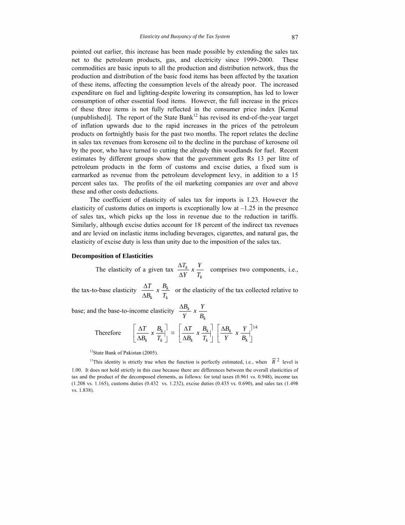
pointed out earlier, this increase has been made possible by extending the sales tax net to the petroleum products, gas, and electricity since 1999-2000. These commodities are basic inputs to all the production and distribution network, thus the production and distribution of the basic food items has been affected by the taxation of these items, affecting the consumption levels of the already poor. The increased expenditure on fuel and lighting-despite lowering its consumption, has led to lower consumption of other essential food items. However, the full increase in the prices of these three items is not fully reflected in the consumer price index [Kemal (unpublished)]. The report of the State Bank12 has revised its end-of-the-year target of inflation upwards due to the rapid increases in the prices of the petroleum products on fortnightly basis for the past two months. The report relates the decline in sales tax revenues from kerosene oil to the decline in the purchase of kerosene oil by the poor, who have turned to cutting the already thin woodlands for fuel. Recent estimates by different groups show that the government gets Rs 13 per litre of petroleum products in the form of customs and excise duties, a fixed sum is earmarked as revenue from the petroleum development levy, in addition to a 15 percent sales tax. The profits of the oil marketing companies are over and above these and other costs deductions.

The coefficient of elasticity of sales tax for imports is 1.23. However the elasticity of customs duties on imports is exceptionally low at –1.25 in the presence of sales tax, which picks up the loss in revenue due to the reduction in tariffs. Similarly, although excise duties account for 18 percent of the indirect tax revenues and are levied on inelastic items including beverages, cigarettes, and natural gas, the elasticity of excise duty is less than unity due to the imposition of the sales tax.

Decomposition of Elasticities

The elasticity of a given tax k

k

TYx

YT∆∆ comprises two components, i.e.,

the tax-to-base elasticity k

k

k TBx

BT

∆∆ or the elasticity of the tax collected relative to

base; and the base-to-income elasticity k

k

BYx

YB∆

Therefore ⎥⎦

⎤⎢⎣

⎡∆∆

k

k

k TBx

BT ≡ ⎥

⎦

⎤⎢⎣

⎡∆∆

k

k

k TBx

BT 14

⎥⎦

⎤⎢⎣

⎡∆

k

k

BYx

YB 13

12State Bank of Pakistan (2005). 13This identity is strictly true when the function is perfectly estimated, i.e., when 2R level is

1.00. It does not hold strictly in this case because there are differences between the overall elasticities of tax and the product of the decomposed elements, as follows: for total taxes (0.961 vs. 0.948), income tax (1.208 vs. 1.165), customs duties (0.432 vs. 1.232), excise duties (0.435 vs. 0.690), and sales tax (1.498 vs. 1.838).

Faiz Bilquees

88

Where

T = tax revenue, Y = GDP, and Bk = base related to individual categories of taxes.

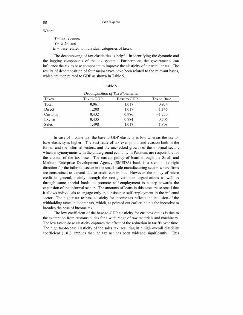
The decomposing of tax elasticities is helpful in identifying the dynamic and the lagging components of the tax system. Furthermore, the governments can influence the tax to base component to improve the elasticity of a particular tax. The results of decomposition of four major taxes have been related to the relevant bases, which are then related to GDP as shown in Table 5.

Table 5

Decomposition of Tax Elasticities Taxes Tax to GDP Base to GDP Tax to Base Total 0.961 1.017 0.934 Direct 1.208 1.017 1.146 Customs 0.432 0.986 –1.250 Excise 0.435 0.984 0.706 Sales 1.498 1.017 1.808

In case of income tax, the base-to-GDP elasticity is low whereas the tax-to-

base elasticity is higher. The vast scale of tax exemptions and evasion both in the formal and the informal sectors, and the unchecked growth of the informal sector, which is synonymous with the underground economy in Pakistan, are responsible for the erosion of the tax base. The current policy of loans through the Small and Medium Enterprise Development Agency (SMEDA) bank is a step in the right direction for the informal sector in the small scale manufacturing sector, where firms are constrained to expand due to credit constraints. However, the policy of micro credit in general, mainly through the non-government organisations as well as through some special banks to promote self-employment is a step towards the expansion of the informal sector. The amounts of loans in this case are so small that it allows individuals to engage only in subsistence self-employment in the informal sector. The higher tax-to-base elasticity for income tax reflects the inclusion of the withholding taxes in income tax, which, as pointed out earlier, blunts the incentive to broaden the base of income tax.

The low coefficient of the base-to-GDP elasticity for customs duties is due to the exemption from customs duties for a wide range of raw materials and machinery. The low tax-to-base elasticity captures the effect of the reduction in tariffs over time. The high tax-to-base elasticity of the sales tax, resulting in a high overall elasticity coefficient (1.81), implies that the tax net has been widened significantly. This

Elasticity and Buoyancy of the Tax System

89

includes the imposition of the sales tax on electricity, gas, and petroleum products, with consequent adverse effects on the already poor. Elasticities of the three components for excise duties are less than unity. Low tax collection relative to the base is attributable mainly to replacement of excise duty by the sales tax. However, at the same time, cheaper smuggled as well as imported goods have flooded the domestic markets, resulting in loss of revenues to the government on account of excise duty and sales tax.

Overall, the low base-to-income elasticities, as well as the relatively lower tax-to-base elasticities, explain the low elasticities of the various taxes. They reflect the failure of the successive governments to improve the tax administration. Efforts to improve the tax imposition and implementation have been beset with loopholes to allow evasion in one form or another. Furthermore, “ad hocisim” in policy measures to enhance revenues has resulted in distortions and narrow bases with consequent decline in revenues.

The findings of this study can be compared with earlier studies to show that the low elasticities have been inherent in the Pakistani tax system for a long time. Of the six studies reviewed here, four have similar findings, which are attributed to low tax-to-base elasticities. The study by Khan (1974) for the period 1960-61 to 1971-72 estimates the elasticity and buoyancy of the tax system using the Dummy Variable method. In this study, elasticites exceed buoyancy for total tax revenues, excise duties, and income tax. However, elasticities for sales tax, customs duties, and income tax from manufacturing are less than unity but still exceed the buoyancy coefficients. It appears that this study is beset with all the problems associated with this method as described in Section III. The coefficient of customs duties is puzzling because it was the main source of revenues until late 1980s. The study by Jeetun (1978) uses Khan’s data-set extended by four years to estimate the buoyancy and elasticity by the Proportional Adjustment Method, and his findings differ significantly from those of Khan. He reports less than unity elasticity for all taxes with different bases except for customs duties with GDP base. Furthermore, they are less than the buoyancy estimates. He attributes these results to low tax-to-base elasticities particularly for income tax, which is supposed to be progressive. In the case of Pakistan, Jeetun rightly argues that progressivity is lost to various concessions and exemptions, besides a weak tax administration and widespread evasion. These findings are confirmed by the present study despite the use of a different methodology and the different time-period covered. This confirms that the distortions prevailing in the tax system in the 1960s still persist.

Gillani (1986) uses both the proportional adjustment and the Divisia Index methods to estimate the elasticity and buoyancy of taxes for the period 1972 to 1982. The results of this study are closer to those of Khan’s study, it shows high elasticity coefficients for all taxes except for export taxes on account of the two methodologies used. However, the gaps in the methodologies make a systematic analysis difficult.

Faiz Bilquees

90

The estimates of elasticity and buoyancy by Kemal (1995) over the period 1971 to 1992, based on the Proportional Adjustment Method, coincide with those of Jeetun and the present study. The buoyancy coefficients exceed the elasticity coefficients by a wide margins. As compared to this study, the coefficients of elasticity are relatively lower because they do not capture the impact of the reforms initiated in the early 1990s.

V. CONCLUSIONS AND POLICY RECOMMENDATIONS

The estimates of buoyancy and elasticity based on the Divisia Index approach show that overall the use of discretionary measures has been relied upon significantly as a source of revenue augmentation in Pakistan. The low elasticites of the tax system reported by earlier studies using a different methodology confirm the existence of continued exemptions, allowances, and loopholes for evasion. All these factors contribute to distortions in the tax system, preventing the tax base to broaden as the economy expands. The reforms in the tax structure since late 1990s—in terms of a relatively cleaner administration facilitating the tax-payers—and the broadening of the sales tax base are visible. However, the efforts to increase the share of direct taxes are at best extremely limited. Inclusion of the withholding tax as a part of direct tax reflects an artificial increase in the share of income tax, which has adverse implications for a genuine increase in income tax revenues, as for expanding the tax net.

Broadening of the sales tax base in a relatively short period is a positive development. However, at the same time, the imposition of sales taxes on petroleum products and utilities ignores its adverse impact on the already poor segments of the population.

The reduction in the tariff rates over time affects the coefficient of elasticity for imports significantly. However, the decline in the customs duty coefficients is picked up by the sales tax revenue from imports. The decline in revenues from the excise duties is also predictable considering the extension of sales tax to a large number of sectors/commodities. This decline is captured by the coefficient of sales tax on domestic output.

Overall, it appears that taxes are being levied without due consideration to equity issues. For example, the capital gains on equity remain exempted from tax on the pretext of developing stock markets; therefore the billions being earned from the stock market bubble remain untaxed, while sales tax on petroleum products and utility prices has overburdened the common man. This has directly affected the common man with limited resources.

The easy way to realise revenues—through sales tax on petroleum products and rising utility prices—has equity implications; a higher sales tax rate on luxury items could be used to prevent, or at least reduce, the taxation of the essential and basic inputs to the production and distribution processes. This would help increase

Elasticity and Buoyancy of the Tax System

91

production, output, and hence employment. High cost of production has been a major factor inhibiting investment, besides procedural and institutional delays. This calls for a better coordination between the revenue department, investment ministry, and other relevant departments. In this regard, serious note should be taken of the State Bank of Pakistan report which has not only revised the end-of-fiscal-year target of inflation due to the massive increase in oil price (which includes levy of customs, excise, and sales tax besides the petroleum development levy). It also points out that the decline in revenues of sales tax from kerosene oil, which is mainly used as fuel by the poor, is due to the decline in its sale. The report maintains that these people are turning to woodlands for fuel. This reflects the lack of communication between the Ministry of Environment and the tax authority.

The revenue department, working in isolation, is focussing only on more revenue generation from the direct taxes by including withholding tax (WHT) in the income tax, and from indirect taxes by levying a uniform sales tax on all items regardless of the possible negative outcomes. For an effective outcome of its reform package, it needs to consider the consequences of its policies for other departments, as well as the long-run consequences of short-term measures to achieve a rapid increases in direct and indirect taxes. This calls for a consultative process in policy formulation, which is generally lacking at all levels.

APPENDIX I

TESTS FOR STATIONARITY

The first step in time-series analysis is the test for stationarity. If a variable is stationary, i.e., it does not have a unit root, it is said to be I(0)—integrated of order zero. If a variable is not stationary on level but stationary in its first-differenced form, it is said to be integrated of order one, or (1). The presence of unit root in a univariate time-series is tested by the Augmented Dicky-Fuller regression (1979 and 1981) of the form:

∆Yt =a0+βt+γYt–1 + ΣPi=2 βi ∆Yt–i+1+ εt

Where

γ = –[1–Σ p i=1ai], βi = Σj=i p aj

∆ is first difference of Yt , a0 is the stochastic term that follows the classical assumptions—it has zero mean, constant variance, and is non-auto-correlated, or is white noise.

The null hypothesis H0 : γ = 0 implies that the time-series is non-stationary; The alternative hypothesis, H0 : γ = 0, implies that the time-series is stationary. We estimate the equation by the OLS and compare the t-ratios of the

estimated co-efficient of Yt–1 with the Dicky-Fuller table. If the computed absolute value of tau statistics exceeds the DF critical tau (τ) values, we reject the hypothesis

Faiz Bilquees

92

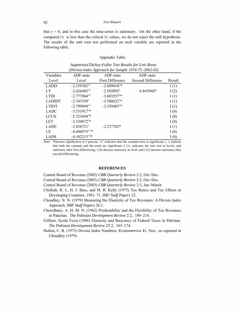
that γ = 0, and in this case the time-series is stationary. On the other hand, if the computed |τ| is less than the critical |τ| values, we do not reject the null hypothesis. The results of the unit root test performed on each variable are reported in the following table.

Appendix Table

Augmented Dickey-Fuller Test Results for Unit Roots (Divisia Index Approach for Sample 1974-75–2002-03)

Variables Level

ADF-stats Level

ADF-stats First Difference

ADF-stats Second Difference Result

LADD –2.359382c,t –2.699034c* I (1) LY –2.626483c,t –2.565092c –6.843948* I (2) LTDI –2.777864c,t –3.603557c* I (1) LADIDT –2.743358c –3.588622c* I (1) LTIDT –2.799894c,t –3.359485c* I (1) LADC –3.551917c* I (0) LCUS –5.723694c* I (0) LET –3.330872c* I (0) LADE –2.858721c –2.237782* I (1) LS –4.496973c, t* I (0) LADS –4.102213c,t* I (0)

Note: *Denotes significance at 5 percent, “c” indicates that the constant term is significant; c, t, indicate that both the constant and the trend are significant; I (1), indicates the unit root in levels, and stationary after first differencing; I (0) denotes stationary at level; and I (2) denotes stationary after second differencing.

REFERENCES

Central Board of Revenue (2002) CBR Quarterly Review 2:2, Oct–Dec. Central Board of Revenue (2003) CBR Quarterly Review 2:2, Oct–Dec. Central Board of Revenue (2003) CBR Quarterly Review 2:3, Jan–March. Chelliah, R. J., H. J. Bass, and M. R. Kelly (1975) Tax Ratios and Tax Efforts in

Developing Countries, 1961–71. IMF Staff Papers 22. Choudhry, N. N. (1979) Measuring the Elasticity of Tax Revenues: A Divisia Index

Approach. IMF Staff Papers 26:1. Chowdhury, A. H. M. N. (1962) Predictability and the Flexibility of Tax Revenues

in Pakistan. The Pakistan Development Review 2:2, 189–214. Gilllani, Syeda Fizza (1986) Elasticity and Buoyancy of Federal Taxes in Pakistan.

The Pakistan Development Review 25:2, 163–174. Hulten, C. R. (1973) Divisia Index Numbers. Econometrica 41, Nov., as reported in

Choudhry (1979).

Elasticity and Buoyancy of the Tax System

93

IMF (2001) IMF Country Report No. 01/1178. International Monetary Fund, Washington, D. C.

Jeetun, Azad (1978) Buoyancy and Elasticity of Taxes in Pakistan. Applied Economics Research Centre (AERC), Karachi. (Research Report No. 27.)

Kemal, A. R. (1995) Pakistan: A Profile of the Tax System. In Issues and Experiences in Tax System Reforms in Selected Countries of the ESCAP Region. New York: United Nations.

Kemal, A. R. (1999) Elasticity and Buoyancy of the Tax System and the Incidence of Taxes. (Unpublished.)

Kemal, M. Ali (2003) Underground Economy and Tax Evasion in Pakistan: A Critical Evaluation. Pakistan Institute of Development Economics, Islamabad. (Research Report No.184.)

Khan, M. Z. (1973) Responsiveness of Tax Yield to Increases in National Income. The Pakistan Development Review 12:4, 416–432.

Musgrave, Richard A. (1959) The Theory of Public Finance. New York: McGraw Hill.

Pakistan, Government of (Various Issues) Pakistan Economic Survey. Islamabad: Economic Advisers Wing, Ministry of Finance.

Pakistan, Government of (Various Issues). CBR Yearbook. Islamabad: Directorate of Research and Statistics, Central Board of Revenue.

Star, Spencer, and Robert E. Hall (1976) An Approximate Divisia Index of Total Factor Productivity. Econometrica 44, March, as reported in Choudhry (1979).

State Bank of Pakistan (2001-02) Annual Report of the State Bank of Pakistan. Karachi.

State Bank of Pakistan (2005) The State of Pakistan’s Economy: Second Quarterly Report for the Year 2004-2005 of the Central Board of State Bank of Pakistan. Karachi.