effect of oil price and exchange rate …ijecm.co.uk/wp-content/uploads/2017/02/5218.pdfeffect of...

International Journal of Economics, Commerce and Management United Kingdom Vol. V, Issue 2, February 2017

Licensed under Creative Common Page 312

http://ijecm.co.uk/ ISSN 2348 0386

EFFECT OF OIL PRICE AND EXCHANGE RATE VOLATILITY

ON ECONOMIC GROWTH IN NIGERIA

Akindele John Ogunsola

Department of Economics, Ekiti State University, Ado-Ekiti, Nigeria

[email protected], [email protected]

Gbenga Dayo Olofinle

College of Postgraduate Studies, Department of Economics,

Obafemi Awolowo University, Ile-Ife, Nigeria

[email protected]

Paul Adeniyi Adeyemi

Department of Economics, Ekiti State University, Ado-Ekiti, Nigeria

[email protected]

Abstract

Controversies abound over the nexus between oil price and exchange rate volatility on

economic growth. However, previous related studies in Nigeria only focused on either the

impact of oil price shock on economic growth or the effect of exchange rate volatility on

economic growth without examining the joint effect of the two variables on economic growth.

The study equally examined the dynamic relationship that exists among oil price, exchange rate

volatility and economic growth in Nigeria. Secondary data were used for this study. The

variables are real gross domestic product, exchange rate, money supply and inflation rate which

were sourced from Central Bank of Nigeria (CBN) Statistical Bulletin, while oil price was sourced

from energy price indicator. The econometric techniques employed were co-integration analysis

and vector autoregressive model. The result showed that oil price volatility has negative but

insignificant relationship with economic growth as 1 per cent increase in oil price volatility

reduces real gross domestic product by 1.7 per cent. In the same vein, exchange rate volatility

has insignificant adverse effect on real GDP as 1 percent increase in exchange rate volatility

brings about 2.6 per cent decrease in real GDP. The study concluded that oil price volatility

http://ijecm.co.uk/

http://ijecm.co.uk/

International Journal of Economics, Commerce and Management, United Kingdom


depresses economic growth more than volatility in exchange rate, a scenario that may attribute

to mismanagement of oil revenue in the country. Based on the findings of this study, it was

recommended that there should be a reduction in the proportion of expenditure on imported

commodities by Nigerians and urges them to patronise locally made goods.

Keywords: Oil Price, Exchange Rate, Economic Growth, Impulse Response, Variance

Decomposition

INTRODUCTION

It has been observed that exchange rate plays an increasingly significant role in any economy

as it directly affects domestic price level, competiveness of traded goods and services,

allocation of resources, productive capacity of goods and services and investment decision

Odusola (2003). Besides, Exchange rate is a key variable in the context of general economic

policy making as its appreciation or depreciation affects the performance of other

macroeconomic variables in any economy. In the light of its importance, every country pays so

much attention to the appropriateness of her foreign exchange policy and the stability of the

exchange rate becomes the formidable bedrock of all economic activities. Since the adoption of

the Structural Adjustment Programme (SAP) in July, 1986, Nigeria has moved to various types

of floating regimes of exchange rate from the fixed/pegged regimes between 1960s and the

mid-1980s. Floating exchange rate has been shown to be preferable to the fixed arrangement

because of the responsiveness of the rates to the foreign exchange market Nwankwo (1980).

Exchange rate volatility is a risk associated with unexpected changes in exchange rate, this is

caused by some economic factors such as inflation rate, interest rate, and balance of payments

Ozturk (2006). Crude oil became an export commodity in Nigeria in 1958 following the discovery

of the first producible well in 1956. The discovery of crude oil in Nigeria led to what is commonly

referred to as the “Dutch disease”. The Dutch Disease (DD) refers to the paradoxical deleterious

consequence of natural resource booms on the countries where they occur. The concept was

coined from the experience of Netherlands in the 60s when, as a result of exploitation of the

newly discovered large deposit of natural gas in the North Sea, the non-oil tradable sector

became less competitive and declined, Olusi and Olagunju (2005). Thus, the performance of the

manufacturing sector remained less impressive and that of agriculture declined. In the early

1960s, manufacturing activities consisted of partial processing of agricultural commodities,

textiles, breweries, cement, rubber processing, plastic products, and brick making. The

economy gradually became dependent on crude oil as productivity declined in other sectors.

http://ijecm.co.uk/

© Ogunsola, Olofinle & Adeyemi

Licensed under Creative Common 14

As a mono-product economy, Nigeria remains susceptible to the movements in international

crude oil prices. During periods of favourable oil price shocks triggered by conflicts in some oil -

producing areas of the world, the surge in the demand for the commodity by consuming nations,

seasonality factors, trading positions, etc; the country experiences favourable terms-of-trade

quantified in terms of a robust current account surplus and exchange rate appreciation. On the

converse, when crude oil prices are low, occasioned by factors such as low demand,

seasonality factors, oil glut and exchange rate appreciation, the Nigerian economy experiences

significant drop in the level of foreign exchange inflows that often result in budget deficit and or

slower growth.

It is observed that a significant number of studies have looked at the relationship

between oil price and selected macroeconomic variables (including exchange rate) in both

developed and developing countries. Some studies surveyed reported positive result, while

some reported negative result. Some of the studies even show no relationship. Though, the

work of Aliyu (2009) assessed the impact of oil price shock and exchange rate volatility on

economic growth, his study did not capture the recent fluctuations in oil price between 2008 and

2009. Hence, this study differs from the early studies conducted in relation to the investigation of

the impact of oil price shock on the economic growth in many ways. (a) updating the data so as

to capture the recent fluctuations in oil price between 2008 and 2012. (b) method of data

analysis, using VAR instead of VEC. (c) examine the impact of oil price and exchange rate on

economic growth at disaggregated level, and (d) examine the dynamic interrelationship that

exists among the variables since it is possible or the variable in the model to affect one another.

It is against this background that this study intends to fill these gaps.

The rest of the paper is organised as follows: section two is on literature review. Section

three presents the methodology, while section four discusses the results. Section five concludes

and makes recommendations.

LITERATURE REVIEW

Brief Empirical Literature

Hang et al (2005) examines the effect of oil price change and its volatility on economic activities

in the United State, Canada, and Japan. Their findings show that when oil price change and

volatility exceed a threshold, they possess significant explanatory power for the outcome

variables such as industrial production and stock market return.

Milani (2009) estimates a structural general equilibrium model to examine the changing

relationship between oil price and macroeconomic variables to fit the data on the United State

using quarterly series for the 1960:1- 2008:1sample. His findings suggest that oil price affect the



economy through an additional channel, i.e, through their effect on the formation of agent

beliefs. The estimated learning dynamics indicates that economic agent‟s perceptions about the

effect of oil price on the economy have change over time. Oil price were perceived to have large

effects on output and inflation in the 1970s, but only a milder effect after the mid-1980.

Al-Mulali, (2010) examines the impact of oil price shocks on the real exchange rate and

the gross domestic product in Norway using time series data from 1975 to 2008. The vector

auto-regressive has been implemented using the co-integration and the granger causality test.

The results of the study show that the increase in oil price is the reason behind Norway‟s GDP

increase and the increase of its competitiveness to trade by its real exchange rate depreciation.

Daussa (2008) investigates the significant impact of exchange rate shock on prices of

Malaysians imports and exports. In methodology, the study adopts error correction (ECM)

model and prices of export covering the period of 1999 to 2006. Exchange rate significantly

affects the fluctuation of import prices. These results imply that import prices are more sensitive

than export prices to shock in nominal exchange rates. Shock in nominal exchange rates,

however, does not give significant impact on both export prices and money supply.

Olomola and Adejumo (2006) in their empirical study on the oil price shock and

aggregate economic activity in Nigeria used a VAR model with quarterly data from 1970 to

2003. Volatility was measured as the conditional variance of the percentage change of the

nominal oil price. The five variables used for the empirical study were real gross domestic

product, proxied by industrial production index (y), domestic money supply, the real effective

exchange rate (REER), the inflation rate (CPI), and real oil price. The specification used for the

model is the scaled specification, a non-linear transformation of oil price that takes volatility into

account. The findings showed that while oil prices significantly influence exchange rate, it does

not have significant effect on output and inflation in Nigeria. They concluded that an increase in

the price of oil results in wealth effects which appreciates the exchange rate and increases the

demand for non-tradable, a situation that would result in “Dutch disease”.

Aliyu (2009) assesses the impact of oil price shock and real exchange rate volatility on

the real gross domestic product in Nigeria using quarterly data that span the period 1986-2007.

He used the Johansen VAR-based co integration technique to examine the sensitivity of real

GDP to change in oil prices and real exchange rate volatility in the long-run while the vector

error correction model was used in the short-run. The result of the long-run analysis indicated

that a 10.0 per cent permanent increase in crude oil prices increases the real GDP by 7.72 per

cent, similarly a 10.0 per cent appreciation in exchange rate increases GDP by 0.35 per cent.

The short-run dynamic was found to be influenced by the long-run equilibrium condition. He

recommended the diversification of the economy and infrastructural diversification.

http://ijecm.co.uk/



Ayadi (2005) analyses directly the effects of oil-price shocks for Nigeria over the 1980-2004

periods employing standard VAR. This VAR process is similar to Ayadi, et al (2000), that the

responses of the macroeconomic variables- output, inflation, and the real exchange rate- to oil-

price shocks are small. More precisely, the contributions of the oil price shock to the variance of

output, inflation and real exchange rate are 1.1 and 0 percent at impact respectively, and about

7.1 and 5 percent after a year. In comparison, the contributions of the oil price shock to the

variance of oil prices are 100 percent at impact and about 97 percent after a year.

Mordi (2006) contends that exchange rate volatility in Nigeria is explained by

fundamentals such output growth (GDP) rates, inflation, balance of payments position, external

reserves, interest rates movements, external debt position, productivity and other

macroeconomic shocks.

Ogun (2004) analyses the effects of real exchange rate misalignment and volatility on

the growth of non-oil exports. It is found that irrespective of the alternative measures of

misalignment adopted, both real exchange rate misalignment and volatility adversely affected

growth of Nigeria‟s non-oil export.

THEORETICAL FRAMEWORK AND METHODOLOGY

Solow Growth Model

Since the objective of the study is to examine the relationship between oil price, exchange rate

volatility and economic growth, following Rasche and Tatom (1977), the study adopts the Solow

growth model. Over the years, the growth theory has evolved as a major feature of economic

growth and development. In analysing the impact of oil price and exchange rate volatility on

economic growth, Solow‟s model of economic growth is premised on the proposition that output

in an economy is produced by a combination of labour (L) and capital (K), under constant

returns to scale, so that doubling input results in doubling output. Contemporary versions

distinguish between physical and human capital. Thus, the quantity of output (Y) is also

determined by inputs which capital and labour are employed. Or mathematically:

𝑌 = 𝐴𝑓(𝐾, 𝐿) (3.1)

Solow assumed that this production function exhibits constant returns to scale, that is, if all

inputs are increased by a certain multiple, output will increase by exactly the same multiple.

The Solow neoclassical growth model uses a standard aggregate production function in which

𝑌𝑡 = 𝐴𝐾𝑡𝛼𝐿𝑡

1−𝛼 𝑤𝑕𝑒𝑟𝑒0 < 𝛼 < 1 (3.2)

In this case, Y is gross domestic product, K is stock of capital, Lis labour and assumed to grow

at n+ g

𝐿𝑡 = 𝐿0𝑒𝑛𝑡 (3.3)



𝐴𝑡 = 𝐴0𝑒𝑔𝑡 (3.4)

The number of effective units of labour, At Lt grows at rate n+g.

The model assumes that a constant fraction of output, s, is invested. Defining k as the stock of

capital per effective unit of labour, k=K/AL and y as the level of output per effective unit of

labour, y = Y/AL, the evolution of k is governed by:

𝐾𝑡 = 𝑠𝑦𝑡 − (𝑛 + 𝑔 + 𝛿)𝑘𝑡 (3.5)

Where 𝛿 is the “rate of depreciation”, equation (3.5) above implies that k converges on steady-

state value k* defined by

𝐾∗(〔 𝑠

𝑛+𝑔+𝛿 〕)

1

1−𝛼 (3.6)

This implies that the steady-state capital-labour ratio is related positively to the rate of saving

and negatively to the rate of population growth. The central predictions of the Solow model

concern the impact of saving and population growth on real income. Substituting (3.6) into the

production function and taking logs, we find that steady-state income per capita is

𝑙𝑛𝑌𝑡

𝐿𝑡= 𝐴0 + 𝑔𝑡 −

𝛼

1−𝛼ln(𝑛 + 𝑔 + 𝛿) (3.7)

The magnitudes alongside the signs of the coefficients on savings and population growth are

predicted based on the fact that the model assumes that factors are paid their marginal products

In the case of competitive markets being assumed, the growth rate of the economy is seen as a

weighted sum of growth rates of efficiency parameter gA and of the capital stock gK.The weights

on labour and capital are the shares of payment to labour and capital in Gross Domestic

Product (GDP).

𝑔𝑦 = 𝑔𝐴 + 𝛼1𝑔𝐿 + 𝛼𝑘 𝑔𝑘 (3.8)

The Solow Growth model assumes that the marginal product of capital decreases with the

amount of capital in the economy. In the long run, as the economy accumulates more and more

capital,𝑔𝐾, approaches zero and the growth rate is determined by technical progress and growth

in the labour force. However, in the short run, an economy that accumulates capital faster will

enjoy a higher level of output. The above argument relates to the entire economy, but can also

be extended to sub sectors of the economy such as education.

According to the traditional neoclassical growth theory, output growth results from one or three

(3) factors: increases in labour quality and quantity (through population growth and education),

increases in capital (through saving and investment), and improvement in technology Todaro

and Smith (2004).

It is important to note that A is not fixed, but varies with different production functions based on

the factors being studied. This production function is widely used in the literature; including

Smyth (1993); Fosu (1990), and Fosu and Aryeetey (2008). Apart from the traditional input of

http://ijecm.co.uk/



production, the model also assumes other conventional inputs. Literature on economic growth

indicates that, there are multitudes of potential variables that can affect the TFP (A) in equation

(3.2).

However, in order to provide appropriate linkage among the chosen variable, various channels

through which change in the price of crude oil affects the growth of an economy have been

identified in the literature on crude oil and economic growth. Channels identified in the literature

include the supply side effect, inflation effect, and the real balance effect Brown and Yücel

(2002): Jiménez-Rodríguez and Sánchez (2005): Chuku, et al (2010) and Bhanumurthy, et al,

(2012).

Model Specifications

This study employs vector autoregressive (VAR) methodology to study the effect of oil price

volatility and exchange rate volatility on economic growth in Nigeria. The model is specified as:

𝑅𝐺𝐷𝑃 = 𝑂𝐼𝐿𝑃𝑉𝑂,𝐸𝑋𝑅𝑉𝑂 (3.9)

Realizing the importance of the influence of monetary variables on output in this kind of study,

the authors incorporate inflation rate (INFR) and money supply (M2) into the model as control

variables. The inclusion of these variables rests on the ground that they influence the economic

growth in any country. Hence, equation (3.1) becomes:

𝑅𝐺𝐷𝑃 = (𝑂𝐼𝐿𝑃𝑉𝑂,𝐸𝑋𝑅𝑉𝑂, 𝐼𝑁𝐹𝑅,𝑀2) (3.10)

Expressing equation (3.2) in its explicit form, it becomes:

𝑅𝐺𝐷𝑃𝑡 = 𝛼𝑂 + 𝛼1𝑂𝐼𝐿𝑃𝑉𝑂𝑡 + 𝛼2𝐸𝑋𝑅𝑉𝑂𝑡 + 𝛼3𝐼𝑁𝐹𝑅𝑡 + 𝛼4𝑀2𝑡 + 𝜖𝑡 (3.11)

Where 𝑅𝐺𝐷𝑃𝑡 = real gross domestic product at time t,

𝑂𝐼𝐿𝑃𝑉𝑂𝑡 = oil price volatility at time t,

𝐸𝑋𝑅𝑉𝑂𝑡= exchange rate volatility at time t,

𝐼𝑁𝐹𝑅𝑡 = inflation rate at time t,

𝑀2𝑡 = broad money supply at time t and

𝜖𝑡 = stochastic term.

𝛼𝑖 = parameters to be estimated (𝑖 = 0, 1, 2, 3, 4)

Utilizing the variables in equation (3.3), a VAR model is specified thus:

𝑋𝑡 = 𝛼 + 𝛽1𝑋𝑡−1 + 𝛽2𝑋𝑡−2 +⋯ 𝛽𝑞𝑋𝑡−𝑘 + 𝜇𝑡 (3.12)

Where 𝑋𝑡 = {RGDP, OILPVP, EXRVO, INFR, M2}

It should be noted that 𝑋𝑡 is a k x 1-dimensional vector of the endogenous variables, 𝛼 is a k x

1-dimentional vector of constant and 𝛽1 … 𝛽𝑞 are k x k dimensional autoregressive coefficient



matrices while 𝜇𝑡 is a k x 1-dimensional vector of the stochastic error term which is normally

distributed with the following properties:

𝐸(𝜇𝑡) = 0, 𝐸(𝜇𝑡𝜇𝑡′ ) = 𝜃 and 𝐸 𝜇𝑡𝜇𝑡

′ = 0,

if 𝑖 ≠ 𝑗.

Thus, equation (3.4) can be expressed in matrix form as follows:

𝑋𝑋𝑡−1...𝑋𝑡−𝑘+1

=

𝛼0...0

+

𝛽1 𝛽2

1 0

. .

. .𝛽𝑞−1 𝛽𝑞

0 0. 1. .

. .1 .

. .

. .. .0 0

. 1

. .

. .1 0

𝑋𝑡−1

𝑋𝑡−2...𝑋𝑡−𝑘

+

𝜇𝑡0...0

(3.13)

In a compact form, equation (3.5) can be re-stated as follows:

𝑋𝑡 = 𝛼 + Γ𝑖𝑋𝑡−𝑘𝑘

𝑖=1+ 𝜇𝑡 (3.14)

𝑖 = 1, 2… k.

Sources of Data

We made use of the secondary data for all the variables involved in this study. The data for all

these variables are sourced from the Central Bank of Nigeria (CBN) Statistical Bulletin, the

National Bureau of Statistics (NBS) and World Development indicator (WDI). Specifically, the

data on real gross domestic product (RGDP), real exchange rate, money supply and inflation

rate are extracted from CBN (2012) in conjunction with NBS. However, the data on oil price are

extracted from the review of world energy publications

ANALYSIS AND RESULTS

Phillip-Perron (PP) Unit Root Test

Table 1: Result of Unit Root Test on Variables with both Constant alone and Constant and

Linear Trend: Phillip-Perron (PP) Test

Variables Intercept/Constant Intercept and linear trend Remarks

PP Test Critical Value PP Test Critical Value

RGDP -5.1458

(0.0001)

1% = -3.6009

5% = -2.9350

10% = -2.6058

-5.9006

(0.0001)

1% = -4.1985

5% = -3.5236

10% = -3.1929

I(1)

OILPVO -14.4643

(0.0000)

1% = -3.6010

5% = -2.9350

10% = -2.6058

-16.8213

(0.0000)

1% = -4.1985

5% = -3.5236

10% = -3.1929

I(1)

http://ijecm.co.uk/



EXRVO -5.3471

(0.0001)

1% = -3.6010

5% = -2.9350

10% = -2.6058

-5.7399

(0.0001)

1% = -4.1985

5% = -3.5236

10% = -3.1929

I(1)

INFR -9.6058

(0.0000)

1% = -3.6010

5% = -2.9350

10% = -2.6058

-8.5689

(0.0000)

1% = -4.1985

5% = -3.5236

10% = -3.1929

I(1)

M2 -3.3003

(0.0213)

1% = -3.6210

5% = -2.9450

10% = -2.6058

-3.1763

(0.1929)

1% = -4.1985

5% = -3.5236

10% = -3.1929

I(1)

As portrayed by the unit root test result in Table 1, all the examined variables are integrated of

order one, I(1). The implication of this order is that the time-series variables used in this study

are non-stationary at their level forms, but are only stationary after their first difference. This

indicates that we can proceed to co-integration analysis.

Co-integration Test Result

Now that we realise that our time-series data are made up of variables that are I(1), the next

task is to test for the existence of co-integration, or otherwise, among the variables.

Table 2: Co-Integrating Results (with a linear trend) where r is the

number of co-integrating vectors

Lag interval (1 to 1)

Trace Test Max-Eigen Test

Null Alternative Statistic Critical

Value (5%)

Null Alternative Statistic Critical

Value (5%)

r = 0 r = 1 46.84076 69.81889 r = 0 r = 1 17.56709 33.87687

r ≤ 1 r = 2 29.27367 47.85613 r ≤ 1 r = 2 11.84446 27.58434

r ≤ 2 r = 3 17.42921 29.79707 r ≤ 2 r = 3 9.041459 21.13162

r ≤ 3 r = 4 8.387752 15.49471 r ≤ 3 r = 4 7.708712 14.26460

r ≤ 4 r = 5 0.679040 3.841466 r ≤ 4 r = 5 0.679040 3.841466

Trace test indicates no co-integrating

equation at the 0.05 level.

Max-Eigen test indicates no co-integrating

equation at the 0.05 level.

Since the co-integration result in Table 2 indicates non-existence of co-integrating equation,

then the choice of estimating Vector Error Correction Model (VECM) is automatically discarded.

Hence, the estimation of the Vector Autoregressive (VAR) Model becomes imperative.

Table 1...



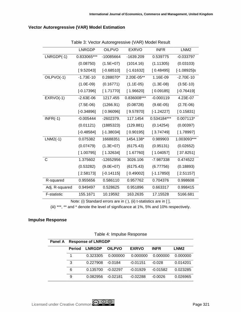
Vector Autoregressive (VAR) Model Estimation

Table 3: Vector Autoregressive (VAR) Model Result

LNRGDP OILPVO EXRVO INFR LNM2

LNRGDP(-1) 0.833065***

(0.08750)

[ 9.52043]

-10085664

(1.5E+07)

[-0.68510]

-1639.209

(1014.16)

[-1.61632]

0.539775

(1.11305)

[ 0.48495]

-0.033797

(0.03103)

[-1.08925]s

OILPVO(-1) -1.73E-10

(1.0E-09)

[-0.17396]

0.288070*

(0.16771)

[ 1.71770]

2.20E-05**

(1.1E-05)

[ 1.96620]

1.16E-09

(1.3E-08)

[ 0.09185]

-2.70E-10

(3.5E-10)

[-0.76419]

EXRVO(-1) -2.63E-06

(7.5E-06)

[-0.34896]

1217.455

(1266.91)

[ 0.96096]

0.836008***

(0.08728)

[ 9.57870]

-0.000119

(9.6E-05)

[-1.24227]

4.23E-07

(2.7E-06)

[ 0.15831]

INFR(-1) -0.005444

(0.01121)

[-0.48584]

-2602379.

(1885323)

[-1.38034]

117.1454

(129.881)

[ 0.90195]

0.534184***

(0.14254)

[ 3.74749]

0.007113*

(0.00397)

[ 1.78997]

LNM2(-1) 0.075382

(0.07479)

[ 1.00795]

16688351

(1.3E+07)

[ 1.32634]

1454.138*

(6175.43)

[ 1.67760]

0.989903

(0.95131)

[ 1.04057]

1.003093***

(0.02652)

[ 37.8251]

C 1.375602

(0.53282)

[ 2.58173]

-12652956

(9.0E+07)

[-0.14115]

3026.106

(6175.43)

[ 0.49002]

-7.987338

(6.77756)

[-1.17850]

0.474522

(0.18893)

[ 2.51157]

R-squared 0.955656 0.586110 0.957762 0.704376 0.998608

Adj. R-squared 0.949497 0.528625 0.951896 0.663317 0.998415

F-statistic 155.1671 10.19592 163.2635 17.15528 5166.681

Note: (i) Standard errors are in ( ), (ii) t-statistics are in [ ],

(iii) ***, ** and * denote the level of significance at 1%, 5% and 10% respectively.

Impulse Response

Table 4: Impulse Response

Panel A Response of LNRGDP

Period LNRGDP OILPVO EXRVO INFR LNM2

1 0.323305 0.000000 0.000000 0.000000 0.000000

3 0.227908 -0.0184 -0.01151 -0.028 0.014201

6 0.135700 -0.02297 -0.01929 -0.01582 0.023285

9 0.082956 -0.02181 -0.02288 -0.0026 0.026965

http://ijecm.co.uk/



10 0.071010 -0.02132 -0.02353 0.000487 0.027575

Panel B Response of OILPVO


1 -2144021 54350229 0.000000 0.000000 0.000000

3 -4797549 5341311. 7432667. -7480001 2246499.

6 -6710199 2739289. 5551726. 939149.7 2786697.

9 -6601545 1877101. 3323607. 2620085. 3402294.

10 -6363531 1540472. 2708796. 2792210. 3563798.

Panel C Response of EXRVO


1 -72.5772 136.0534 3743.945 0.000000 0.000000

3 -1034.29 1424.474 2561.166 480.8914 341.1470

6 -1638.72 941.5736 1616.568 563.3065 725.6866

9 -1712.49 549.4160 959.3221 730.3231 945.4498

10 -1672.07 443.7184 781.8434 767.8791 996.1247

Panel D Response of INFR


1 -0.12838 0.156228 -0.69523 4.048239 0.000000

3 0.286053 -0.10791 -0.8155 1.096196 0.158396

6 0.486151 -0.34759 -0.63134 0.132214 0.136446

9 0.509442 -0.29764 -0.46992 -0.00705 0.076898

10 0.500278 -0.27332 -0.42528 -0.02355 0.060076

Panel E Response of LNM2


1 0.012663 -0.013 -0.0122 -0.00489 0.112430

3 -0.00622 -0.02896 -0.02169 0.043133 0.113194

6 -0.01499 -0.03356 -0.03947 0.063526 0.114520

9 -0.01285 -0.03977 -0.05215 0.066140 0.114136

10 -0.01101 -0.04155 -0.05537 0.065984 0.113605

Cholesky Ordering: LNRGDP OILPVO EXRVO INFR LNM2

As portrayed in Table 4, Panel A indicates how real GDP responds to shock in other variables in

the model. It is, however, observed in the Panel that real GDP does not respond to shock in any

of the other variables in the first year, as real GDP solely responds to its own shock in this first

period. One standard deviation shock in oil price persistently decreases real GDP throughout

the periods as from the second year. Hence, the response of real GDP to shock in oil price

conforms with a priori expectation. This result buttresses the VAR result that there is inverse

Table 2...



relationship between oil price volatility and real GDP. The result is at variance with studies by

Jin (2008), Aliyu (2009) and Agbede (2012) which find significant positive relationship between

oil price and real GDP. Also from Table 4, Panel B demonstrates how oil price volatility

responds to shock in other variables in the estimated model. One standard deviation shock in

real GDP brings about a persistent decrease in oil price volatility, even though mixed responses

are expected. Conversely, the oil price volatility shows a persistent increase to shock in

exchange rate volatility throughout the periods. The relationship experienced here is in

conformity with a priori expectation.

Panel C of Table 4 captures how exchange rate volatility responds to shock in other

variables in the model. The second objective of the study which is to examine the effect of oil

price volatility on exchange rate volatility is catered for in this Panel. Panel C shows that one

standard deviation shock in oil price volatility brings about a persistent increase in exchange

rate volatility throughout the periods in accordance with a priori expectation. This implies that an

unexpected increase in oil price volatility increases the exchange rate volatility and vice-versa.

Appendix 1 also buttresses the information presented in Table 4.

Variance Decomposition

Table 5: Variance Decomposition

Panel A Variance Decomposition of LNRGDP:

Period S.E. LNRGDP OILPVO EXRVO INFR LNM2

1 0.323305 100.0000 0.000000 0.000000 0.000000 0.000000

3 0.482101 99.04744 0.203623 0.077872 0.553389 0.117673

6 0.564336 97.70325 0.623533 0.336620 0.836155 0.500446

9 0.594241 96.47864 0.984062 0.711545 0.800114 1.025642

10 0.599944 96.05389 1.091672 0.851918 0.785039 1.217485

Panel B Variance Decomposition of OILPVO:


1 54392501 0.155375 99.84463 0.000000 0.000000 0.000000

3 59357094 1.115975 91.20744 2.646293 4.787132 0.243159

6 61845353 4.150617 84.70806 5.640995 4.750036 0.750296

9 63808108 7.232175 79.93843 6.517190 4.846885 1.465317

10 64359746 8.086344 78.63127 6.583092 4.952375 1.746924

Panel C Variance Decomposition of EXRVO:


1 3747.119 0.037515 0.131833 99.83065 0.000000 0.000000

http://ijecm.co.uk/



3 5966.336 4.150874 10.57575 83.60872 1.262632 0.402026

6 7683.600 13.88827 12.74419 69.05023 2.114865 2.202439

9 8781.101 22.07217 11.54527 58.24329 3.422394 4.716877

10 9071.583 24.07862 11.05697 55.31578 3.923231 5.625395

Panel D Variance Decomposition of INFR:


1 4.112478 0.097448 0.144315 2.857944 96.90029 0.000000

3 4.927696 0.468799 0.205512 7.559325 91.61203 0.154335

6 5.204381 2.592033 1.278597 12.15876 83.57240 0.398210

9 5.387034 5.096360 2.252528 14.16691 78.01457 0.469631

10 5.434164 5.855875 2.466608 14.53469 76.66908 0.473742

Panel E Variance Decomposition of LNM2:


1 0.114641 1.220082 1.286094 1.132856 0.181838 96.17913

3 0.208336 0.463167 3.945843 1.988206 5.656490 87.94629

6 0.316514 0.736709 4.729692 4.364418 13.04409 77.12509

9 0.405371 0.811129 5.491451 6.935981 15.84565 70.91579

10 0.431855 0.779743 5.764118 7.755177 16.29624 69.40472

Cholesky Ordering: LNRGDP OILPVO EXRVO INFR LNM2

Variance Decomposition

Panel A of Table 5 reveals that real GDP‟s own shock solely accounts for all (100%) its forecast

error variance in the first year but its influence slightly decreases in the longer horizons as it still

accounts for 96% in the tenth year. Thus, oil price volatility, exchange rate volatility, inflation rate

and money supply all account for negligible proportion of real GDP forecast error variance

throughout the periods. Each of oil price volatility and money supply barely contributes more

than 1% while each of exchange rate volatility and inflation rate accounts for less than 1% all

through. However, all the other variables (apart from inflation rate) still have the tendency of

contributing more in the longer horizons as their respective influences increase throughout the

periods while inflation rate reaches its peak of 0.84% in the sixth year and starts declining in the

longer horizons. This suggests that every of the variables in the model have influence on one

another. However, this also confirms the results of the VAR model above, as it can be seen

from the panel A of table 5. Apart from own shock, the most dominant variable is oil price.

Panel B of Table 5 shows that exchange rate volatility dominates the forecast error

variance of oil price volatility in most of the periods as it dominates from the fifth year to the

eighth year while real GDP becomes dominant as from the ninth year, even though their

Table 5...



respective contributions are very close to each other throughout the periods. It is observed here

that the contributions of real GDP, exchange rate volatility and money supply to the forecast

error variance in oil price volatility increase over the years while the contribution of inflation rate

oscillates in the horizons (it increases from 0% in the first year to its peak of 4.96% in the fourth

year and then decreases in the longer horizons The simple meaning of this is that exchange

rate volatility has significant influence on oil price volatility than every other variables in the

model in the short horizon, While real gross domestic product influences oil price volatility more

in the model in the longer horizon.

Furthermore, Panel C of Table 5 reveals that oil price volatility is the most important

source of forecast error variance in exchange rate volatility for the first five years as it reaches

its peak of 12.76% in the fifth year while its influence slightly decreases in the longer horizons

as it declines to 11.06% in the tenth year. Appendix 2 equally provides additional information

about the result presented in Table 6.

CONCLUSION AND RECOMMENDATIONS

The study investigates the effect of oil price and exchange rate volatility on Nigerian economic

growth and the findings of the study are summarised as follows:

One standard deviation shock in oil price volatility persistently decreases real GDP

throughout the periods. This result buttresses the VAR result that there is inverse relationship

between oil price volatility and economic growth. The implication of all these is that the income

effect of the rising oil price is not felt while the output effect is prevalent in the country.

Similarly, the response of real GDP to shock in exchange rate volatility elicits a

persistent decline in real GDP. This result also gives credence to the VAR model result which

portrays a negative and insignificant relationship between exchange rate volatility and economic

growth. However, both oil price volatility and exchange rate volatility account for negligible

proportion of real GDP forecast error variance throughout the periods

In line with the findings of this study, the following recommendations are proposed.

There should be a reduction in the proportion of expenditure on imported commodities by

Nigerians and urges them to patronise locally made goods. Sequel to the scenario above,

coupled with the fact that oil price volatility has adverse effect on economic growth, the study

also recommends effective diversification of the economy which will save the country from the

imminent menace of over-reliance on petroleum. More so, there is urgent need for government

of Nigeria to nip in the bud the rising increase of exchange rate through a mechanism of tighten-

up monetary policy.

http://ijecm.co.uk/



SUGGESTIONS FOR FURTHER STUDIES

This study examines the effect of oil price and exchange rate volatility on economic growth in

Nigeria with focus to determine the impact of each of these two variables on Nigerian economy.

However, it is suggested that this study should be further extended to other areas that will be of

immense relevance to Nigeria such as nexus between exchange rate volatility and industrial

development in Nigeria and also the asymmetric effect of oil price on industrial sector in Nigeria.

REFERENCES

Agbede, M.O., (2012) “The Growth Implications of oil Price Shock in Nigeria‟‟ Journal of Emerging Trends in Economics and Management Sciences (JETEMS) 4(3): 343-349.

Aliyu, S.U.R (2009) „‟ Impact of oil Price Shock and Exchange Rate Volatility on Economic Growth in Nigeria: An Empirical Investigation‟‟ Research Journal of International studies-issue II

Aliyu, S.U.R. (2008) „‟Exchange Rate Volatility and Export Trade in Nigeria: An Empirical Investigation

Al-mulaliUsama, (2010).“The impact of oil price on the exchange rate and economic growth in Norway”.

Ayadi, O.F (2005). “Oil price Fluctuation and the Nigeria Economy OPEC review”, pp 199-212.

Ayadi, O.F, A Chtterjee, and C.P. Obi (2000), “A vector autoregressive Analysis of an oil dependent emerging Economy-Nigeria‟‟ OPEC Review, pp.33-349.

Bhanumurtly, N.R., Das, S., and Bose, S. (2012). Oil price shocks, pass-through policy and its impact on India, working paper, National institute of public Finance and policy, New Delhi.

Brown, S.P., and Yucel, M.k (2002). Energy prices and Aggregate Economic activity: An interpretative Survey. Quarterly review of Economics and finance.

Chuku, A.C, Effiong, I.E, and Sam, R.N (2010).Oil price distortions and their short and long-run impacts on the Nigerian Economy, Retrieved 11 /30/2012, from Mpra.Ub.Unimuenhen.de/ 24434.

Daussa, J. (2008), Impact of exchange rate shock on prices of imports and exports, MPRA paper No.11624, posted 18. Edward, Sebastine (1988), exchange rate misalignment in developing countries. Baltimore, MD. John Hopkins university press.

Hang, B., Hwang M.J., Hsiw-Ping. P, (2005) Price Shocks on economics activities: an application of multivariate threshold model. Energy Economics 27 (3), 455-476.

Jimenez-Rodriquez, R, and Sanchez, M. (2005) oil price shocks and real GDP growth; Empirical Evidence for Some.Applied economics, 37, 201 – 228.

Jin, G (2008) “The impact of oil price shock and Exchange Rate Volatility on Economic Growth: A comparative Analysis for Russia Japan and China‟‟. Research Journal of International studies, issues 8, pp. 98-111

Killian, L. and R.J. Vigfusson(2009). Pitfalls in Estimating Asymetrics Effect of Energy price shocks, CEPR Discussion papers 7234.C.E.P.R. Discussion papers.

Mordi, C.N (2006). “Challenges of Exchange Rate Volatility in Economic Management in Nigeria.”Bullion Vol.30, No.3. July - Sept. 2006.

Nwanko, G.O (1980). The Nigerian financial system Ibadan: Macmillian.

Odusola, A. F. (2003). “Exchange Rate Policy Analysis and Management: Concept and Theoretical issues. Workshop on macroeconomic policy analysis management organized for the staff of Central Bank of Nigeria, August 2003 CBN Training School, Satellite Town, Lagos.

Ogun, O. (2004) real exchange rate behavior and Non-oil Export Growth in Nigeria.African Journal of Economic policy.Vol 11, No 1 June.



Olomola A. and Adejumo (2006): “Oil Price shock and Aggregate Economic Activity in Nigeria,‟‟ African Economic and Business Review, vol 4: 2, ISSN 1109-5609

Olusi J.O. and Olagunju M. A. (2005) "The primary sector of the economy and Dutch Disease in Nigeria''.

Ozturk I, (2006) “Exchange Rate Volatility and Trade: A Literature survey‟‟, International Journal of Applied Econometrics and Quantitative studies, vol 3-1(2006).

Todaro, M.P and S.C. Smith (2004) Economic Development (8th Edition). (India: Pearson Education Ltd). Pp 141-144, 360-417.

APPENDICES

Appendix 1

-.2

-.1

.0

.1

.2

2 4 6 8 10

Response of LNM2 to LNM2

-.2

-.1

.0

.1

.2

2 4 6 8 10

Response of LNM2 to INFR

-.2

-.1

.0

.1

.2

2 4 6 8 10

Response of LNM2 to EXRVO

-.2

-.1

.0

.1

.2

2 4 6 8 10

Response of LNM2 to OILPVO

-.2

-.1

.0

.1

.2

2 4 6 8 10

Response of LNM2 to LNRGDP

-4

-2

0

2

4

6

2 4 6 8 10

Response of INFR to LNM2

-4

-2

0

2

4

6

2 4 6 8 10

Response of INFR to INFR

-4

-2

0

2

4

6

2 4 6 8 10

Response of INFR to EXRVO

-4

-2

0

2

4

6

2 4 6 8 10

Response of INFR to OILPVO

-4

-2

0

2

4

6

2 4 6 8 10

Response of INFR to LNRGDP

-4,000

-2,000

0

2,000

4,000

6,000

2 4 6 8 10

Response of EXRVO to LNM2

-4,000

-2,000

0

2,000

4,000

6,000

2 4 6 8 10

Response of EXRVO to INFR

-4,000

-2,000

0

2,000

4,000

6,000

2 4 6 8 10

Response of EXRVO to EXRVO

-4,000

-2,000

0

2,000

4,000

6,000

2 4 6 8 10

Response of EXRVO to OILPVO

-4,000

-2,000

0

2,000

4,000

6,000

2 4 6 8 10

Response of EXRVO to LNRGDP

-40,000,000

0

40,000,000

80,000,000

2 4 6 8 10

Response of OILPVO to LNM2

-40,000,000

0

40,000,000

80,000,000

2 4 6 8 10

Response of OILPVO to INFR

-40,000,000

0

40,000,000

80,000,000

2 4 6 8 10

Response of OILPVO to EXRVO

-40,000,000

0

40,000,000

80,000,000

2 4 6 8 10

Response of OILPVO to OILPVO

-40,000,000

0

40,000,000

80,000,000

2 4 6 8 10

Response of OILPVO to LNRGDP

-.2

-.1

.0

.1

.2

.3

.4

2 4 6 8 10

Response of LNRGDP to LNM2

-.2

-.1

.0

.1

.2

.3

.4

2 4 6 8 10

Response of LNRGDP to INFR

-.2

-.1

.0

.1

.2

.3

.4

2 4 6 8 10

Response of LNRGDP to EXRVO

-.2

-.1

.0

.1

.2

.3

.4

2 4 6 8 10

Response of LNRGDP to OILPVO

-.2

-.1

.0

.1

.2

.3

.4

2 4 6 8 10

Response of LNRGDP to LNRGDP

Response to Cholesky One S.D. Innovations ± 2 S.E.

http://ijecm.co.uk/



Appendix 2

-.2

-.1

.0

.1

.2

.3

.4

2 4 6 8 10

Response of LNRGDP to LNRGDP

-.2

-.1

.0

.1

.2

.3

.4

2 4 6 8 10

Response of LNRGDP to OILPVO

-.2

-.1

.0

.1

.2

.3

.4

2 4 6 8 10

Response of LNRGDP to EXRVO

-.2

-.1

.0

.1

.2

.3

.4

2 4 6 8 10

Response of LNRGDP to INFR

-.2

-.1

.0

.1

.2

.3

.4

2 4 6 8 10

Response of LNRGDP to LNM2

-40,000,000

0

40,000,000

80,000,000

2 4 6 8 10

Response of OILPVO to LNRGDP

-40,000,000

0

40,000,000

80,000,000

2 4 6 8 10

Response of OILPVO to OILPVO

-40,000,000

0

40,000,000

80,000,000

2 4 6 8 10

Response of OILPVO to EXRVO

-40,000,000

0

40,000,000

80,000,000

2 4 6 8 10

Response of OILPVO to INFR

-40,000,000

0

40,000,000

80,000,000

2 4 6 8 10

Response of OILPVO to LNM2

-4,000

-2,000

0

2,000

4,000

6,000

2 4 6 8 10

Response of EXRVO to LNRGDP

-4,000

-2,000

0

2,000

4,000

6,000

2 4 6 8 10

Response of EXRVO to OILPVO

-4,000

-2,000

0

2,000

4,000

6,000

2 4 6 8 10

Response of EXRVO to EXRVO

-4,000

-2,000

0

2,000

4,000

6,000

2 4 6 8 10

Response of EXRVO to INFR

-4,000

-2,000

0

2,000

4,000

6,000

2 4 6 8 10

Response of EXRVO to LNM2

-4

-2

0

2

4

6

2 4 6 8 10

Response of INFR to LNRGDP

-4

-2

0

2

4

6

2 4 6 8 10

Response of INFR to OILPVO

-4

-2

0

2

4

6

2 4 6 8 10

Response of INFR to EXRVO

-4

-2

0

2

4

6

2 4 6 8 10

Response of INFR to INFR

-4

-2

0

2

4

6

2 4 6 8 10

Response of INFR to LNM2

-.2

-.1

.0

.1

.2

2 4 6 8 10

Response of LNM2 to LNRGDP

-.2

-.1

.0

.1

.2

2 4 6 8 10

Response of LNM2 to OILPVO

-.2

-.1

.0

.1

.2

2 4 6 8 10

Response of LNM2 to EXRVO

-.2

-.1

.0

.1

.2

2 4 6 8 10

Response of LNM2 to INFR

-.2

-.1

.0

.1

.2

2 4 6 8 10

Response of LNM2 to LNM2

Response to Cholesky One S.D. Innovations ± 2 S.E.

effect of oil price and exchange rate …ijecm.co.uk/wp-content/uploads/2017/02/5218.pdfeffect of...

Documents