nexus between exchange rate volatility and oil price ... between exchange rate volatility and oil...

Pak J Commer Soc Sci

Pakistan Journal of Commerce and Social Sciences

2016, Vol. 10 (1), 122-148

Nexus between Exchange Rate Volatility and Oil

Price Fluctuations: Evidence from Pakistan

Rabia Ahmed

Government College University, Faisalabad, Pakistan

E-mail: [email protected]

Imran Qaiser

Department of Economics, Government College University, Faisalabad, Pakistan


Muhammad RizwanYaseen (Corresponding author)

Department of Economics, Government College University, Faisalabad, Pakistan


Abstract

Pakistan experienced too much variation in crude oil prices in the last decades and this

variation received a great attention because it uses all the sectors of the economy. The

purpose of this study is to ascertain the determinants of Real Exchange Rate and analyze

the impact of Real Oil Price Volatility on Real Exchange Rate Volatility in Pakistan over

1983-Q1 to 2014-Q2. Various econometric techniques like Johansen Cointegration and

Vector Error Correction Model have been used for short run and long run analysis

respectively. Our findings explores that productivity differential, real foreign exchange

reserves, interest rate differential, real exports and oil prices are the determinants of

exchange rate. While, Real Foreign exchange reserves volatility, CPI volatility and Real

Oil Price Volatility have positive and NEWS has a negative effect on Real Exchange

Rate Volatility. Volatility results through EGARCH (1, 1) shows the presence of leverage

effect in Real Oil Price Volatility and Real Exchange Rate Volatility. The government

should make suitable policies for equilibrium of oil demand and supply in order to keep

the exchange rate stable. Future research can be made on cross sectional countries by

using monthly data of variables.

Keywords: exchange rate, real exchange rate volatility, oil price fluctuations, impulse

response, exponential generalize autoregressive conditional hetroscedasticity

(EGARCH).

1. Introduction

The exchange rate is an important macroeconomic variable in any economy because it

maintains international competitiveness (Jhingan, 2002). The importance of this variable

can be recognized from the fact that it does play its major role to trim down domestic

price level (Mordi, 2006) but also has an adverse impact on international trade and capital

flows (Abrams, 1980; Hilton, 1984). On the same way, exchange rate volatility has

Ahmed et al.

123

become an imperative issue between developing countries because it creates hurdles to

achieve two main policy maker’s objectives: price stability and economic growth.

Most of the traders produce goods and services and sell them internationally. They

measure their benefits and costs in term of the US Dollar. Similarly, all the developing

countries receive funds, assistances and grants in term of dollar and they reimburse their

money in the same currency. So, US dollar is acceptable in all over the world when

transactions are made internationally. Normally, central bank of a country decides

whether the exchange regime should be fixed or floating. It is important to clear here the

scenario behind the exchange rate in nominal and real term. The real exchange rate can

be distinguished from nominal through the value of county’s product in term of another;

while the price of a currency in term of another is termed as nominal exchange rate.

The phenomenon of volatility can be defined as fluctuations and uncertainty in asset

pricing, portfolio optimization and risk management. Volatility tends to increase if

elasticity of demand and supply is high and vice versa (Obadan, 2006). Exchange rate

volatility is linked with flexible exchange rate. Variability in itself is not a critical

problem. If variability is predicable then volatility has not significant undesirable effect

on international trade and capital flows (Hakkio, 1984).

Pakistan is one of those agrarian based economies that are gradually switching towards

industrialization. This country examined multiple exchange rates since its independence.

Before 1973, there was fixed exchange rate in Pakistan, but after that it was firstly linked

by the pound. History of exchange rate has shown a continuous trend of depreciation

since 1982 to 2001 but this depreciation changed in appreciation in 2002 due to

development and events since 1998. Stability can be seen in the fiscal year 2005-2006.

The average nominal exchange rate was Rs. 91 US dollars from July 2012 to June 2013

and it depreciated by 6.87 percent when exchange rate rose by Rs. 98 US dollar in July

2014. Exchange rate reached to its peak at Rs. 107 US dollars in March 2014 when Loan

has paid for the International Monetary Fund (IMF) Rs. 76.54 million as interest. After

March 2014, exchange rate appreciated to Rs. 101 US dollar till June 2015. The main

reason for this appreciation was a downward trend in oil prices.

Oil market plays a vital role in all sectors of the economy (Azid et al., 2005). Pakistan, as

an oil importing country, experienced large oil price shock (Siddquia a a huge

share2001) and it has huge share of cost of oil in GDP. Its users have less ability to lessen

their consumption. The first oil price shock was observed in 1973 because of the OPEC

oil embargo. The crude oil price was $4.20 per barrel in 1973. Crude oil price remained

constant between 12$ to 14$ per barrel in 1974 to 1978. From 1979 to 1985, oil price

fluctuated due to the Iranian revolution, Iraq war, OPEC quotas, and Iraq invasion of

Kuwait. Their price has been increasing continuously since 2003 and reached at its peak

(126$/barrel) in July 2008. However, after that, a declining trend can be seen. In June

2014, crude oil price was $115/ barrel, but it declines to $50/ barrel in the first month of

2015 that in returns appreciates exchange rate. This appreciation reduces inflation from 8

to 9 percent. This decrease in prices improves import bill by $ 691US million, but this

positive impact vanished when imports of petroleum products increased by 6.3 US$

million. Even though, oil prices in Pakistan reached at its lowest level, but it has not any

positive impact on import bill. The import bill during June 2015 was 12.3$ billion. The

main reason is that exports are decreasing due to energy shortage (GOP, 2015).

Exchange Rate Volatility and Oil Price Fluctuations

124

As the demand for crude oil has been increasing day by day in all over the world, the

influence of oil price on exchange rate and exchange rate volatility will become more and

more obvious. So, it has become more requisite to study further on the impact of oil

price variability on exchange rate fluctuations.

This study contributes to fill the gap in literature regarding oil price variability and

exchange rate fluctuations. This paper explores that oil price is also the key variable that

determine the real exchange rate of Pakistan. The importance of this study is due to the

usage of latest quarterly data from 1983-Q1 to 2014-Q4. In this study, there is the

introduction of new variables like CPI volatility, Real Foreign Exchange Reserves,

NEWS and Oil Price Volatility. These variables used in the studies of oil exporting

countries, but not used in case of Pakistan.

Our study applies EGARCH models to measure exchange rate volatility, CPI Volatility,

Real Foreign Exchange reserves and Oil Price Volatility. EGARCH models are free for

non-negativity constraints and leverage effect can be analyzed from these models. On the

other hand, former studies used ARDL, ARCH, GARCH, IGARCH and TGARCH,

models to measure volatility in case of Pakistan. These models measure the symmetric

effect in conditional variance only and they do not provide any idea about good news or

bad news.

This paper explores the determinant of real exchange rate and the significance of this

study can be stated as it will help us to find whether oil price volatility have any impact

on exchange rate volatility or not in the presence of control variables like CPI volatility,

Real Foreign Exchange Reserves and NEWS. Secondly, this study also determines the

influence of regime, political regime and news on exchange rate volatility. After giving

detail overview of the exchange rate and oil prices in the introduction, this paper is

arranged as follows. Second chapter explains the work of other studies related to the

determinants of exchange rate, oil price and its volatility. Third chapter consists of

models, description of the variables, estimation techniques and methodology. Chapter

forth empirically explores the determinants of exchange rate and investigates the impact

of oil price volatility on exchange rate volatility in the context of Pakistan. Finally,

chapter fifth deals with conclusions and policy recommendation to higher authorities.

2. Literature Review

Various researchers explored the factors that affect exchange in the presence of oil price

by using time series as well as cross sectional data. The empirical analysis on the impact

of oil price variability on exchange rate fluctuations has always been a great concern to

macroeconomists. Before discussing the literature review, firstly we will highlight some

theoretical background of exchange rate. RudigerDornbusch (known as monetarist)

presented his Dornbusch Overshooting Hypothesis (sticky price monetary model) or

exchange rate overshooting model in 1976. According to this model, if exchange rate

disturbance is more than its long run response, this situation is called overshoot

(Dornbusch, 1976). Moreover, if a country experience shock (real or nominal), its

exchange rate may start to diverge from its equilibrium level because of purchasing

power parity (PPP) condition. PPP states that prices are rigid in short run and it adjust

slowly in long run. This adjustment of prices directly affects real money balance and

indirectly demand for money. Real money balance increases due to a slower moment of

prices and in order to compete the money balance, interest rate should have to decrease.

Ahmed et al.

125

This will increase the demand for money. When prices settle after the disturbance

happen, exchange rate shifts back to their original position. Interest rate and exchange

rate are attached to the interest rate parity condition. Interest rate differential works as an

ancillary factor to determine exchange rates. This relationship is based on uncovered

interest rate parity condition. This condition states that the anticipated exchange rate and

home and foreign country interest rate should be equal.

In 1964, Balassa- Samuelsson expressed the relationship between equilibrium exchange

rate and productivity. The assumption of Balassa- Samuelssonstates that those sectors

who exports the goods to another market, has higher productivity as compared to those

sectors who have not share in exports. Wages in the tradable sector tend to increase and

put pressure on the wages of non-tradable sector. Thus, wages are expected to rise as a

whole. This increase in wages will raise prices of non-tradable only because tradable

good have one fix price internationally. As a result, home currency real exchange rate

will appreciate.

Hau (2002) proved the theoretical essence of Obstfeld-Rogoff model by finding the

association between trade integration and exchange rate instability. Adubi and

Okunmadewa, (1999), Calderon and Kubota (2009) and Mwangi et al. (2014) verify this

model. These studies conclude that exchange rate volatility has an inverse relationship

with agriculture exports and if the prices are more elastic, then nominal and real shocks

have less impact on the volatility of real exchange rate.

The observed literature showed that there are two main approaches to investigate the

impact of news on exchange rate variability; innovation in interest rate and the difference

between actual interest rate and expected interest rate (Frenkel, 1981). Galati and Ho

(2001) conducted a study on US and Euro area to explore that how much level of daily

movements in euro/dollar determined by about the macroeconomic condition in 1999 to

2000. Results demonstrated that there is an appreciable correlation between

macroeconomic news and daily movements of the euro against the dollar. Stancik (2006)

analyzed on the determinants of exchange rate volatility by six Eastern European

Countries and six central countries. Results confirmed that exchange rate volatility have

largely affected by the news.

The main findings of Hviding (2004) on the panel of 28 countries showed that higher

reserves reduced exchange rate volatility. According to him, higher foreign exchange

reserves reduce the likelihood of currency, lower external borrowing cost and improve

confidence of investors. These findings are similar with respect to Pakistan (Javed and

Farooq, 2009; Khan, 2013). Egert (2002) investigated on Balassa- Samuelsson principle

and found a weak association of productivity differential and exchange rate. To explore

the relationship between exchange rate unpredictability on productivity growth, Aghion

(2009) conducted a study on cross-country panel data (47 countries) that covered the

period from 1970 to 2000. Results revealed that when productivity growth of

undeveloped countries decreased, exchange rate volatility increased due to decrease in

exports.

There are many studies on exchange rate and oil price of Nigeria (oil exporting country)

that showed the positive relationship between them (Corden, 1984; Akram, 2004). On the

same way, oil price fluctuations positively effect on exchange rate volatility in Nigeria

(Selmia et al., 2012; Salisu and Mobolaji, 2013; Ogundipe and Ogundipe, 2013). But


126

Adeniyi et al. (2012) found out the asymmetric effect of oil price on exchange rate

instability of Nigeria by using EGARCH model. These results reported by Cheng et al.,

(2015) in which oil price, exchange rate and electricity price have a causal asymmetric

relationship to each other. Unlike these studies, Babatunde (2015), investigated that oil

price shocks depreciated the exchange rate because Nigerian government import more

refine oil to other countries when oil prices increase. These results were suggested by

Fowowe (2014). Omoniyi & Olawale (2015) used bound testing procedure to explored

the relationship between Nigerian exchange rate, oil price and inflation. Results revealed

that increase in oil prices is associated with the appreciation of the exchange rate and

inflation is linked with depreciation in the long run.

There occurred positive link between the rate of interest and exchange rate volatility

because higher interest rate attracts foreign capital that increased surplus in the balance of

payment thereby appreciated the domestic currency. Moreover, the rate of exchange

depreciated with a rise in inflation of the country because when inflation rises, both

public and private sectors shift their profits to abroad. Demand of foreign currency

increased, which will effect on the domestic currency through depreciation (Messe &

Rose, 1983). Izraf and Aziz (2009) estimated the long run effect of real interest rate

differential, real oil price on exchange rate by using monthly data of eight countries over

the period of 1980 to 2008. Pooled mean group’ results exposed that interest rate

differential negatively correlate to exchange rate in Pakistan. This study also explored

that higher oil price lead to lower exports and consequently has a negative effect on the

value of the exchange rate. This oil price results are consistent with Samara (2009).

Jamali et al. (2011) also investigated on oil price shocks on Pakistan and scrutinized that

it has significantly effect on interest rate and real effective exchange rate.

Asari et al. (2009) considered VECM in order to analyze the relationship between interest

rate and inflation in Malaysia that covers the period from 1999 to 2009. Long run

relationship suggested that inflation negatively correlate with exchange rate volatility

while interest rate positively in the case of Malaysia. These results are consistent with the

study of Danmola (2013). Another study on the Malaysian economy exposed that there

exists asymmetric effect between conditional volatility of oil price; indicating that bad

news have more effect on the conditional volatility of oil prices as compared to good

news (Ahmed and Wadud, 2011)

To explore the relationship between exchange rate and oil price, (Berument et al., 2014)

investigated their relative effectiveness on the prices of petroleum products. By using

weekly data for seven years (2005-2012), they found that depreciation in exchange rate

raised the price of petroleum products, but this increase is comparatively less when oil

price increased in long-run and vice versa in short-run. In order to deal with the

nonlinear causality of oil importing countries (China and India), Bal & Rath (2015)

conduct a study on oil price and exchange rate by using monthly data from 1994 to 2013.

After the confirmation of nonlinear causality between oil price and exchange rate through

the BDS test (for both countries), results found the bi-directional and uni-directional

Granger causality between the variables in India and China respectively.

Earth quake played a vital role by distrubing infrastucture for any economy. Li & Jing

(2015) analyzed the after effects of Japan Earthquake on yen exchange rate and on crude

oil price. This study found that after an Earthquake experienced, exchange rate

appreciated sharply in the short run. This appreciation increased oil prices but in the long

Ahmed et al.

127

run all these changes become stable. Basnet & Upadhyaya (2015) scrutinized on five

Asian countries and examined the impact of oil price volatility on inflation, output and

exchange rate through SVAR model. Results demonstrated that oil price volatility has not

much impact on output because these countries enclosed large inflow of investment and

have enormous exports.

3. Data and Methodology

This section examines the description of variables, availability of data and methodology.

Firstly, we will generate the model and then we illustrate the variables in detail.

3.1 Model specification

3.1.1 First Model

To explore the determinants of exchange rate, Real Exports (REXP), Productivity

Differential (PROD), Interest Rate Differential (DRR), Real Foreign Exchange Reserves

(RFER) and Oil Price (OILP) are taken as independent variable.

RERt = 𝛼𝜊+ 𝛽1REXPt +𝛽2PRODt + 𝛽3DRRt+ 𝛽4RFERt + 𝛽5ROILPt+µ𝑡

Where α, β’s and µ intercepts, slope and white noise error are term respectively.

3.1.2 Second Model

Second model investigates the link between Real Exchange Rate Volatility (RER_VOL)

and Oil Price Volatility (ROILP_VOL). While Real Foreign Exchange Reserves

Volatility (RFER _VOL), NEWS and CPI Volatility (CPI_VOL) are control variables.

RER_VOLt = 𝛼𝜊+ 𝛽1RFER _VOLt + 𝛽2NEWSt + 𝛽3CPI_VOLt + 𝛽4ROILP_VOLt + µ𝑡

Where α, β’s and µ intercepts, slope and white noise error are term respectively.

3.1.3 Third Model

For modeling different NEWS, Regime (REG), and Political Regime (POL_REG) in the

third model, we used dummy variables.

RER_VOLt = 𝛼𝜊 + 𝛽1𝐷NEWSt + 𝛽2RGMt + 𝛽3POL_ REGt+µ𝑡

Where α, β’s and µ intercepts, slope and white noise error are term respectively. Higher

expectations indicate good news and lower expectation shows bad news. If the expected

interest rate differential is greater than the actual interest rate differential then values of

NEWS will be negative, indicates the good news, which results increased in exchange

rate volatility (Frenkle, 1981).

NEWSt = (Home country interest rate – foreign country interest rate)t – Et-1(country

interest rate – foreign country interest rate)t

A dummy variable is considered 1 for positive news and 0 for bad news. Pakistan has

faced two exchange rate regimes from the period of 1983 to 2014. A dummy variable is

equal to 1 for managing floating exchange rates and for flexible exchange rate it is equal

to zero. Since the independence of Pakistan, different political regime (Marshal Law and

democracy) has been experienced. A dummy variable is equal to 1 for Marshal Law and

0 for democracy.


128

3.2 Definitions of Variables

3.2.1 Real Exchange Rate

The RER is the ratio of nominal exchange rate to CPI. The real exchange rate has taken

in real form because it adjusts the element of inflation and shows more consistency as

compare to nominal exchange rate. It is taken as the dependent variable. The equation of

real exchange rate can be explained as,

RER= 𝑃𝐴𝐾

𝑈𝑆𝐴∗

𝐶𝑃𝐼(𝑈𝑆𝐴)

𝐶𝑃𝐼(𝑃𝐴𝐾)

3.2.2 Real Exports

REXP has been constructed to the ratio of exports and consumer price index. It is

measured in millions of rupees as constructed by Shaheen (2013). According to Jhingan

(2005), if country’s exports exceed then exchange rate appreciates because of an increase

in the demand of its currency and vice versa.

3.2.3 Productivity Differential

PROD is calculated as output per capita of Pakistan in U.S dollar relative to its main

trading partner (U.S). Balassa- Samuelsson (1964) states if output per capita of Pakistan

is higher than U.S, indicates exchange rate appreciation. It is measured in millions of

rupees.

3.2.4 Real Oil Price

ROILP is the ratio of prices of oil in international market per barrel to CPI. An increase

in oil price reduces demand and supply of the economy. The demand of consumers and

producers decreases as the result of reduction in disposable income and supply also

effects because of an increase in the cost of production (Jin, 2008).

3.2.5 News

News variable is calculated as the difference between information prevail at time period t

about the interest rate of home and foreign country and information prevail at time period

t-1 about the expected interest rate of home and foreign country (Frenkle, 1981). In the

second model, if actual interest rate differential is greater than the expected interest rate

differential, it is considered good news because higher actual interest rate shows capital

inflows and vice versa.

3.2.6 Real Foreign Exchange Reserves

RFER includes gold and other central bank assets that are easy to trade in international

financial markets and come entirely within its control (Manchev, 2009). It is calculated in

millions of US$.

3.2.7 Interest Rate Differential

Differential of Real interest rate (DRR) is calculated as

DRRt = 𝑟

𝑟∗

Where r is the real interest rate with respect to home country and r* is real foreign

interest rate with respect to foreign country. If the domestic rate of interest is more than

foreign rate of interest then this results the appreciation of the exchange rate due to the

inflow of foreign capital.

Ahmed et al.

129

3.2.8 Exchange Rate Volatility, CPI Volatility and Real Foreign External Reserves

Volatility

Volatility in exchange rate, CPI and foreign reserves shows the alteration magnitude. The

greater the magnitude of adjustment, more volatile the exchange rates will be. Freely

floating exchange rates are usually volatile. RFER and CPI have also volatile nature

because of dismissive government policies.

3.3 Data Sources and range

This study used data from 1983Q1 (July- September) to 2014Q4 (April 2015- June 2015).

The data of all the variables (above mentioned) are acquired from World development

indicators, International financial statistics, State bank of Pakistan, West Texas Research

Group (WTRG) and Economic Survey of Pakistan (ESP) 2014-15.

3.4 Methodology

This section has great importance because the selection of appropriate methodologies,

which will use further in econometric model, needs great attention. In this study, time

series data (Quarterly) have been utilized that contained so much problem of non-

stationarity. In order to deal with this problem, we used Johansen Cointegration and

VECM. Moreover, the reason of applying this method is that all the variables are

integrated of order 1, while applying ADF. EGARCH (1, 1) has been used to estimate the

volatility of exchange rate, foreign exchange reserves and CPI as reported by Ahmed and

Wadud (2011) andAdeniyi et al. (2012) by applying EViews7 software. GARCH has not

used here because it does not provide any idea on asymmetric effect. Nelson (1991)

measured the asymmetric effect of time varying variance presented EGARCH.

Log (ht2) = α0 + ∑𝑗=1

𝑞αiln|

ɛ𝑡−𝑗

√ℎ𝑡−𝑗| + ∑𝑗=1

𝑞ξ

ɛ𝑡−𝑗

√ℎ𝑡−1 + ∑𝑖=1

𝑝 𝛿 log (ℎ𝑡−𝑖)t

α0 shows the mean equation of EGARCH. αi represents the behavior of volatility due to

shock. The coefficient 𝛿 shows different aspects of shock. If 𝛿 is less than one, indicates

that the data is stationary. The Coefficient ξ shows the asymmetric response of volatility

and informs us about leverage effect. If its value is less than zero, then good news

produces lower volatility than bad news. The term log (ht2) on the left hand side shows

the conditional variance. A significant and negative ξ implies the presence of the

“leverage effect”. After computing volatility, we determined appropriate lag length by

considering VAR (Vector Autoregressive) lag length criteria. Next step is to determine

the number of cointegration equations by using Trace Statistics and Maximum Eigen

values. If the equations are co integrated to each other than the normalized equation may

possibly be used for long run coefficients. In the short run, we must be more concern on

the sign of ECM.

4. Results and Discussions

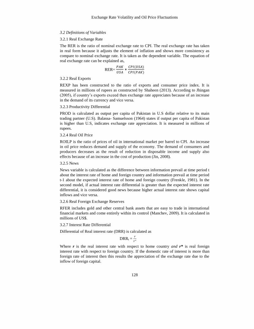
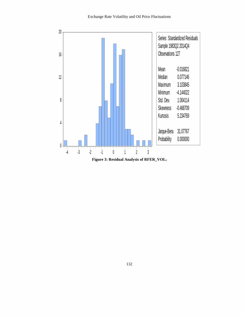
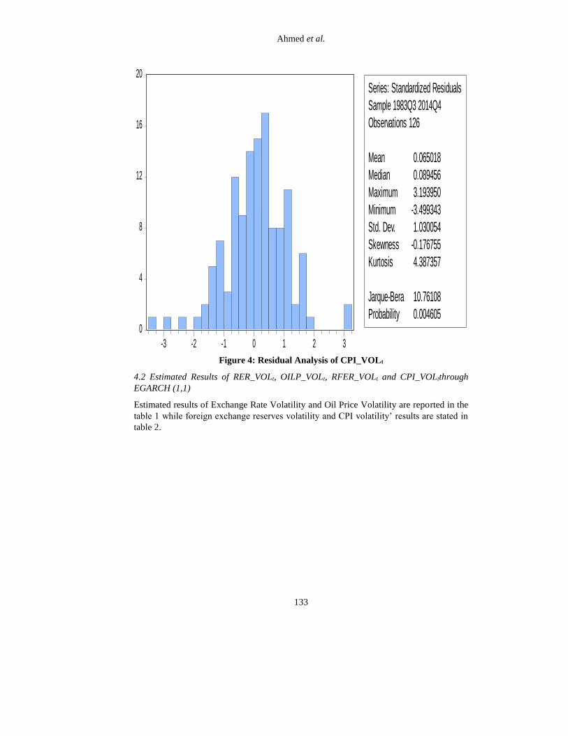
4.1 Residual Analysis through EGARCH

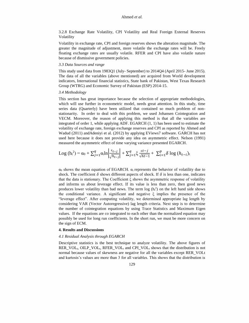
Descriptive statistics is the best technique to analyze volatility. The above figures of

RER_VOLt, OILP_VOLt, RFER_VOLt and CPI_VOLt shows that the distribution is not

normal because values of skewness are negative for all the variables except RER_VOLt

and kurtosis’s values are more than 3 for all variables. This shows that the distribution is


130

leptokurtic. Value of Jarque-Bera are 131.9, 203.9, 31.0, 10.7 for RER_VOLt,

OILP_VOLt, RFER_VOLt and CPI_VOLt respectively, supports that distribution or

residual series are not normal.

Figure 1: Residual Analysis of RER_VOLt

0

4

8

12

16

20

-3 -2 -1 0 1 2 3 4 5

Series: Standardized Residuals

Sample 1983Q3 2014Q4

Observations 126

Mean 0.012907

Median 0.025806

Maximum 5.148933

Minimum -2.777211

Std. Dev. 1.014656

Skewness 0.633466

Kurtosis 7.850508

Jarque-Bera 131.9459

Probability 0.000000

Ahmed et al.

131

Figure 2: Residual Analysis of OILP_VOLt

0

4

8

12

16

20

-5 -4 -3 -2 -1 0 1 2 3



Observations 126

Mean -0.037796

Median 0.026140

Maximum 2.955943

Minimum -5.163741

Std. Dev. 0.997920

Skewness -1.242233

Kurtosis 8.715592




132

Figure 3: Residual Analysis of RFER_VOLt

0

4

8

12

16

20

-4 -3 -2 -1 0 1 2 3



Observations 127

Mean -0.016821

Median 0.077146

Maximum 3.103845

Minimum -4.144022

Std. Dev. 1.004114

Skewness -0.468709

Kurtosis 5.234769



Ahmed et al.

133

Figure 4: Residual Analysis of CPI_VOLt

4.2 Estimated Results of RER_VOLt, OILP_VOLt, RFER_VOLt and CPI_VOLtthrough

EGARCH (1,1)

Estimated results of Exchange Rate Volatility and Oil Price Volatility are reported in the

table 1 while foreign exchange reserves volatility and CPI volatility’ results are stated in

table 2.

0

4

8

12

16

20

-3 -2 -1 0 1 2 3



Observations 126

Mean 0.065018

Median 0.089456

Maximum 3.193950

Minimum -3.499343

Std. Dev. 1.030054

Skewness -0.176755

Kurtosis 4.387357




134

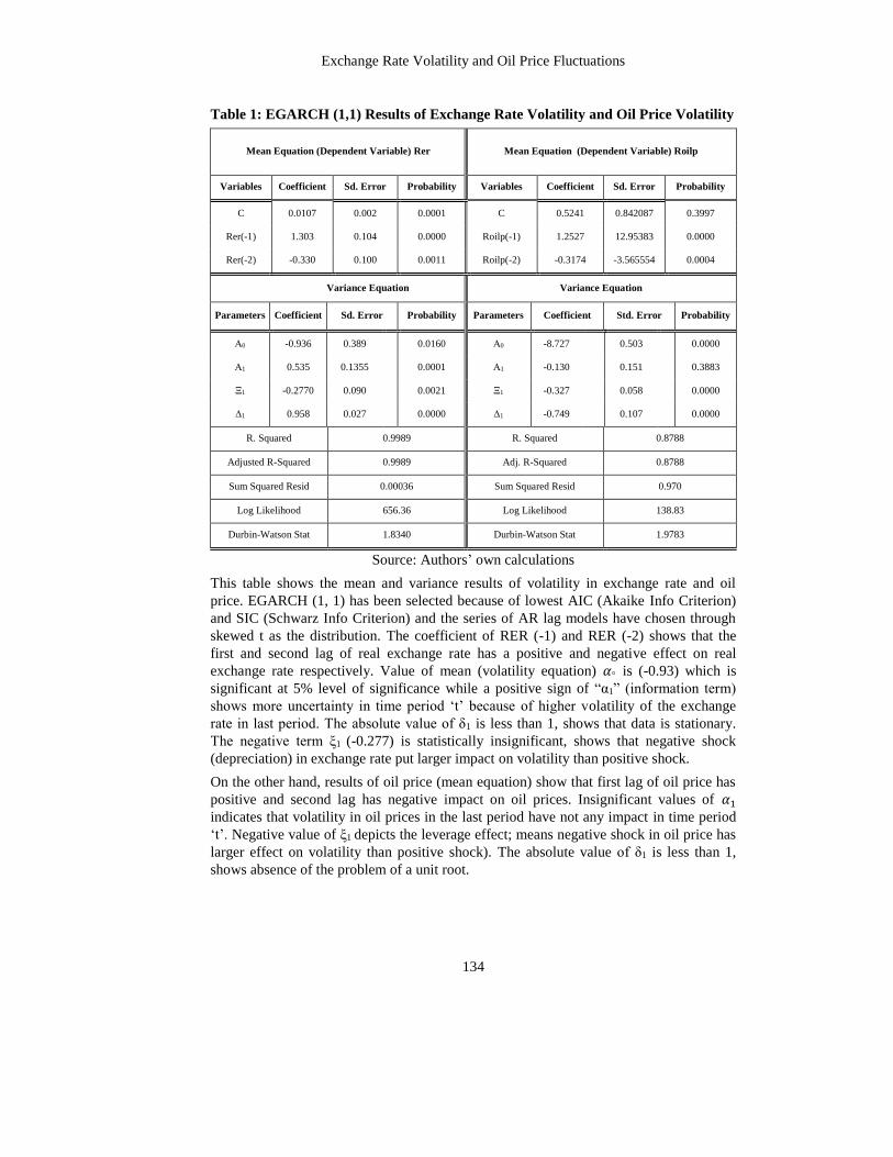
Table 1: EGARCH (1,1) Results of Exchange Rate Volatility and Oil Price Volatility

Mean Equation (Dependent Variable) Rer Mean Equation (Dependent Variable) Roilp

Variables Coefficient Sd. Error Probability Variables Coefficient Sd. Error Probability

C 0.0107

1.303

-0.330

0.002 0.0001 C

Roilp(-1)

Roilp(-2)

0.5241 0.842087 0.3997

Rer(-1) 0.104 0.0000 1.2527 12.95383 0.0000

Rer(-2) 0.100 0.0011 -0.3174 -3.565554 0.0004

Variance Equation Variance Equation

Parameters Coefficient Sd. Error Probability Parameters Coefficient Std. Error Probability

Α0 -0.936 0.389 0.0160 Α0 -8.727 0.503 0.0000

Α1 0.535 0.1355 0.0001 Α1 -0.130 0.151 0.3883

Ξ1 -0.2770 0.090 0.0021 Ξ1 -0.327 0.058 0.0000

Δ1 0.958 0.027 0.0000 Δ1 -0.749 0.107 0.0000

R. Squared 0.9989 R. Squared 0.8788

Adjusted R-Squared 0.9989 Adj. R-Squared 0.8788

Sum Squared Resid 0.00036 Sum Squared Resid 0.970

Log Likelihood 656.36 Log Likelihood 138.83

Durbin-Watson Stat 1.8340 Durbin-Watson Stat 1.9783

Source: Authors’ own calculations

This table shows the mean and variance results of volatility in exchange rate and oil

price. EGARCH (1, 1) has been selected because of lowest AIC (Akaike Info Criterion)

and SIC (Schwarz Info Criterion) and the series of AR lag models have chosen through

skewed t as the distribution. The coefficient of RER (-1) and RER (-2) shows that the

first and second lag of real exchange rate has a positive and negative effect on real

exchange rate respectively. Value of mean (volatility equation) 𝛼° is (-0.93) which is

significant at 5% level of significance while a positive sign of “α1” (information term)

shows more uncertainty in time period ‘t’ because of higher volatility of the exchange

rate in last period. The absolute value of δ1 is less than 1, shows that data is stationary.

The negative term ξ1 (-0.277) is statistically insignificant, shows that negative shock

(depreciation) in exchange rate put larger impact on volatility than positive shock.

On the other hand, results of oil price (mean equation) show that first lag of oil price has

positive and second lag has negative impact on oil prices. Insignificant values of 𝛼1

indicates that volatility in oil prices in the last period have not any impact in time period

‘t’. Negative value of ξ1 depicts the leverage effect; means negative shock in oil price has

larger effect on volatility than positive shock). The absolute value of δ1 is less than 1,

shows absence of the problem of a unit root.

Ahmed et al.

135

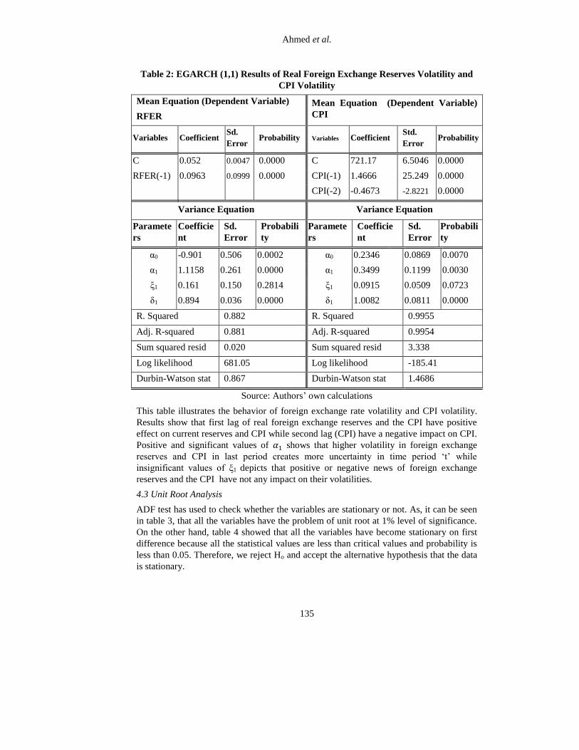
Table 2: EGARCH (1,1) Results of Real Foreign Exchange Reserves Volatility and

CPI Volatility

Mean Equation (Dependent Variable)

RFER

Mean Equation (Dependent Variable)

CPI

Variables Coefficient Sd.

Error Probability Variables Coefficient

Std.

Error Probability

C 0.052

0.0963

0.0047 0.0000 C

CPI(-1)

CPI(-2)

721.17 6.5046 0.0000

RFER(-1) 0.0999 0.0000 1.4666 25.249 0.0000

-0.4673 -2.8221 0.0000

Variance Equation Variance Equation

Paramete

rs

Coefficie

nt

Sd.

Error

Probabili

ty

Paramete

rs

Coefficie

nt

Sd.

Error

Probabili

ty

α0 -0.901 0.506 0.0002 α0 0.2346 0.0869 0.0070

α1 1.1158 0.261 0.0000 α1 0.3499 0.1199 0.0030

ξ1 0.161 0.150 0.2814 ξ1 0.0915 0.0509 0.0723

δ1 0.894 0.036 0.0000 δ1 1.0082 0.0811 0.0000

R. Squared 0.882 R. Squared 0.9955

Adj. R-squared 0.881 Adj. R-squared 0.9954

Sum squared resid 0.020 Sum squared resid 3.338

Log likelihood 681.05 Log likelihood -185.41

Durbin-Watson stat 0.867 Durbin-Watson stat 1.4686


This table illustrates the behavior of foreign exchange rate volatility and CPI volatility.

Results show that first lag of real foreign exchange reserves and the CPI have positive

effect on current reserves and CPI while second lag (CPI) have a negative impact on CPI.

Positive and significant values of 𝛼1 shows that higher volatility in foreign exchange

reserves and CPI in last period creates more uncertainty in time period ‘t’ while

insignificant values of ξ1 depicts that positive or negative news of foreign exchange

reserves and the CPI have not any impact on their volatilities.

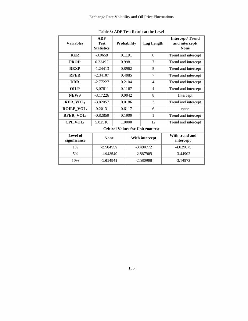
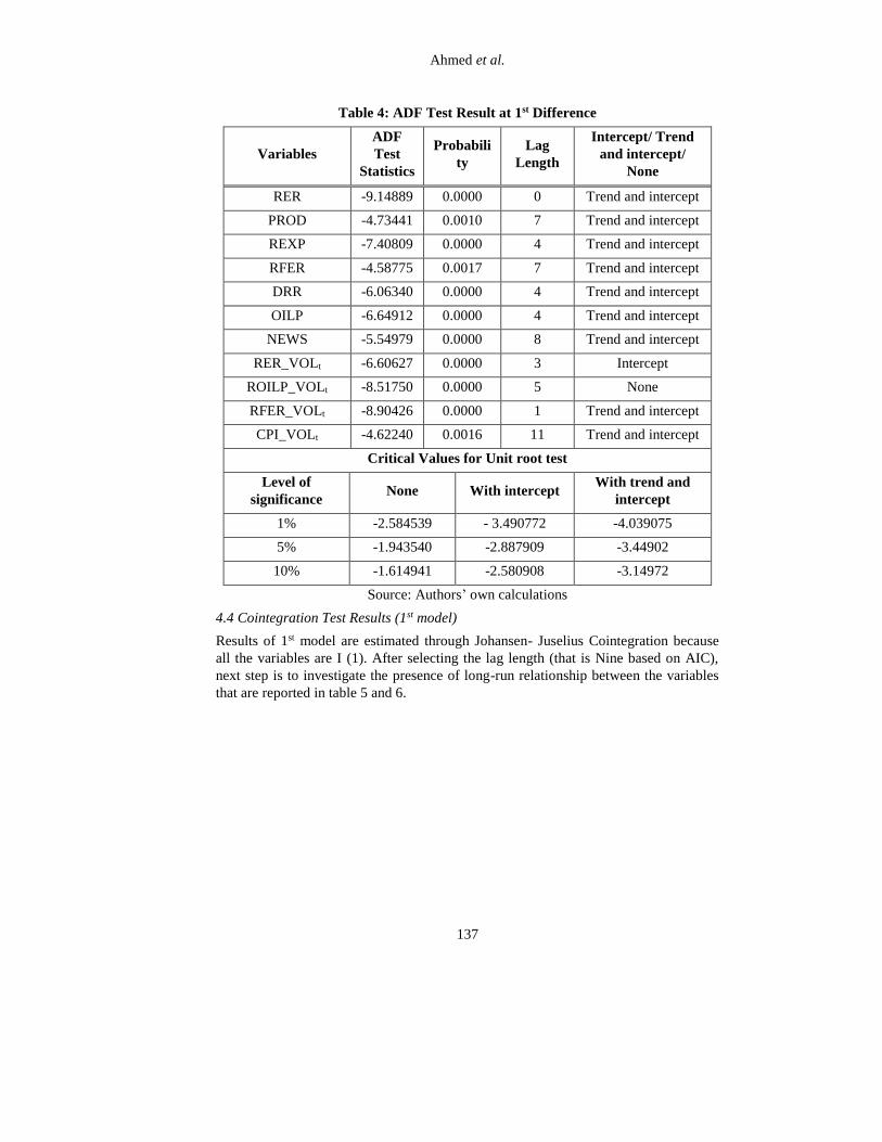
4.3 Unit Root Analysis

ADF test has used to check whether the variables are stationary or not. As, it can be seen

in table 3, that all the variables have the problem of unit root at 1% level of significance.

On the other hand, table 4 showed that all the variables have become stationary on first

difference because all the statistical values are less than critical values and probability is

less than 0.05. Therefore, we reject Ho and accept the alternative hypothesis that the data

is stationary.


136

Table 3: ADF Test Result at the Level

Variables

ADF

Test

Statistics

Probability Lag Length

Intercept/ Trend

and intercept/

None

RER -3.0659 0.1191 0 Trend and intercept

PROD 0.23492 0.9981 7 Trend and intercept

REXP -1.24413 0.8962 5 Trend and intercept

RFER -2.34107 0.4085 7 Trend and intercept

DRR -2.77227 0.2104 4 Trend and intercept

OILP -3,07611 0.1167 4 Trend and intercept

NEWS -3.17226 0.0042 8 Intercept

RER_VOLt -3.82057 0.0186 3 Trend and intercept

ROILP_VOLt -0.20131 0.6117 6 none

RFER_VOLt -0.82859 0.1900 1 Trend and intercept

CPI_VOLt 5.82510 1.0000 12 Trend and intercept

Critical Values for Unit root test

Level of

significance None With intercept

With trend and

intercept

1% -2.584539 -3.490772 -4.039075

5% -1.943540 -2.887909 -3.44902

10% -1.614941 -2.580908 -3.14972

Ahmed et al.

137

Table 4: ADF Test Result at 1st Difference

Variables

ADF

Test

Statistics

Probabili

ty

Lag

Length

Intercept/ Trend

and intercept/

None

RER -9.14889 0.0000 0 Trend and intercept

PROD -4.73441 0.0010 7 Trend and intercept

REXP -7.40809 0.0000 4 Trend and intercept

RFER -4.58775 0.0017 7 Trend and intercept

DRR -6.06340 0.0000 4 Trend and intercept

OILP -6.64912 0.0000 4 Trend and intercept

NEWS -5.54979 0.0000 8 Trend and intercept

RER_VOLt -6.60627 0.0000 3 Intercept

ROILP_VOLt -8.51750 0.0000 5 None

RFER_VOLt -8.90426 0.0000 1 Trend and intercept

CPI_VOLt -4.62240 0.0016 11 Trend and intercept

Critical Values for Unit root test

Level of

significance None With intercept

With trend and

intercept

1% -2.584539 - 3.490772 -4.039075

5% -1.943540 -2.887909 -3.44902

10% -1.614941 -2.580908 -3.14972


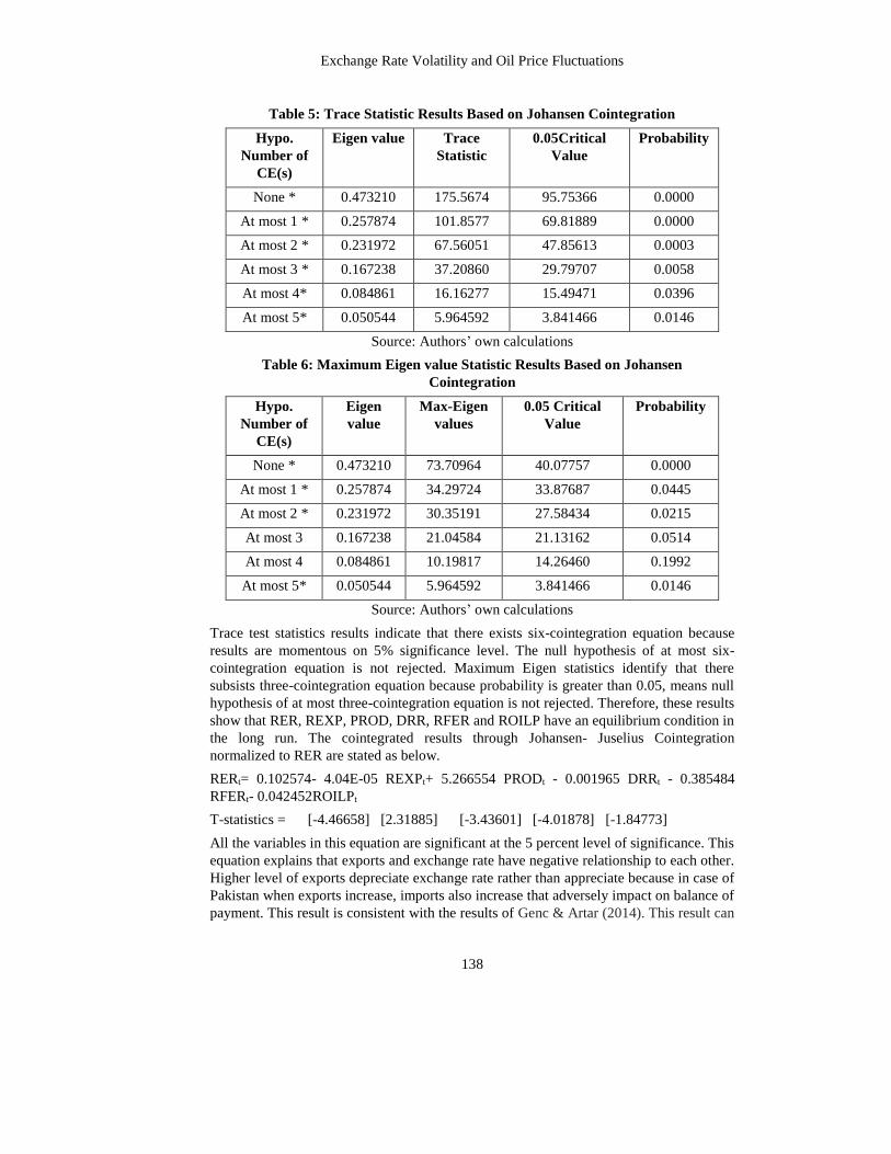
4.4 Cointegration Test Results (1st model)

Results of 1st model are estimated through Johansen- Juselius Cointegration because

all the variables are I (1). After selecting the lag length (that is Nine based on AIC),

next step is to investigate the presence of long-run relationship between the variables

that are reported in table 5 and 6.


138

Table 5: Trace Statistic Results Based on Johansen Cointegration

Hypo.

Number of

CE(s)

Eigen value Trace

Statistic

0.05Critical

Value

Probability

None * 0.473210 175.5674 95.75366 0.0000

At most 1 * 0.257874 101.8577 69.81889 0.0000

At most 2 * 0.231972 67.56051 47.85613 0.0003

At most 3 * 0.167238 37.20860 29.79707 0.0058

At most 4* 0.084861 16.16277 15.49471 0.0396

At most 5* 0.050544 5.964592 3.841466 0.0146


Table 6: Maximum Eigen value Statistic Results Based on Johansen

Cointegration

Hypo.

Number of

CE(s)

Eigen

value

Max-Eigen

values

0.05 Critical

Value

Probability

None * 0.473210 73.70964 40.07757 0.0000

At most 1 * 0.257874 34.29724 33.87687 0.0445

At most 2 * 0.231972 30.35191 27.58434 0.0215

At most 3 0.167238 21.04584 21.13162 0.0514

At most 4 0.084861 10.19817 14.26460 0.1992

At most 5* 0.050544 5.964592 3.841466 0.0146


Trace test statistics results indicate that there exists six-cointegration equation because

results are momentous on 5% significance level. The null hypothesis of at most six-

cointegration equation is not rejected. Maximum Eigen statistics identify that there

subsists three-cointegration equation because probability is greater than 0.05, means null

hypothesis of at most three-cointegration equation is not rejected. Therefore, these results

show that RER, REXP, PROD, DRR, RFER and ROILP have an equilibrium condition in

the long run. The cointegrated results through Johansen- Juselius Cointegration

normalized to RER are stated as below.

RERt= 0.102574- 4.04E-05 REXPt+ 5.266554 PRODt - 0.001965 DRRt - 0.385484

RFERt- 0.042452ROILPt

T-statistics = [-4.46658] [2.31885] [-3.43601] [-4.01878] [-1.84773]

All the variables in this equation are significant at the 5 percent level of significance. This

equation explains that exports and exchange rate have negative relationship to each other.

Higher level of exports depreciate exchange rate rather than appreciate because in case of

Pakistan when exports increase, imports also increase that adversely impact on balance of

payment. This result is consistent with the results of Genc & Artar (2014). This result can

Ahmed et al.

139

be explained as 1 percent increase in exports leads to 4.04 percent depreciation in the

exchange rate in long run. Results of productivity differential and exchange rate show

positive correlation to each other; indicated that increase in productivity differential leads

to appreciation in exchange rate. This appreciation proved Balassa-Samuelson principle.

This result is consistent with the study of Razi et al. (2012). Similarly, there exist a

negative relationship between interest rate differential and exchange rate. 1 percent

increase in interest rate differential (r/r*) depreciates the exchange rate by .0019 percent

because increase of interest rate reduces the demand for money that plunges the value of

currency. This finding is matched with Izraf & Aziz (2009). Significant results of foreign

exchange reserves show that 1 million increases in RFER lead to 0.385 percent

depreciation of the exchange rate as results suggested by Khan (2013). This depreciation

of exchange rate is due to increase in reserves through aid, grant, Extended Fund Facility

(EFF) and loans that IMF paid to Pakistan. Results also show that 1 percent increase in

oil price leads to 0.04 percent depreciates the exchange rate. This result is similar to the

finding of Izraf & Aziz (2009), Ahmed & Wadud (2011), Krugman (1983), Salisu &

Mobolaji (2013). This result verifies Dornbusch Model. Theoretically, Dornbusch (1976)

stated that if a country experience shock (real or nominal), its exchange rate may start to

diverge from its equilibrium level because of purchasing power parity condition and

depreciates the exchange rate.

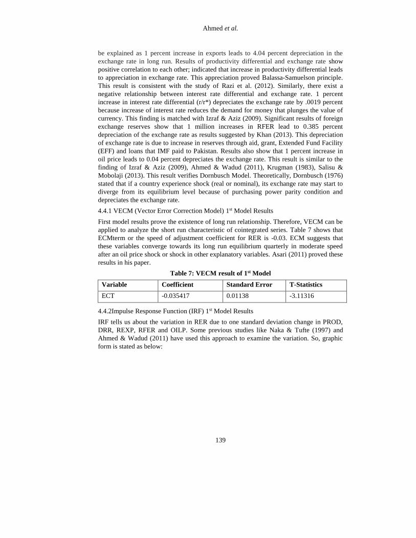
4.4.1 VECM (Vector Error Correction Model) 1st Model Results

First model results prove the existence of long run relationship. Therefore, VECM can be

applied to analyze the short run characteristic of cointegrated series. Table 7 shows that

ECMterm or the speed of adjustment coefficient for RER is -0.03. ECM suggests that

these variables converge towards its long run equilibrium quarterly in moderate speed

after an oil price shock or shock in other explanatory variables. Asari (2011) proved these

results in his paper.

Table 7: VECM result of 1st Model

Variable Coefficient Standard Error T-Statistics

ECT -0.035417 0.01138 -3.11316

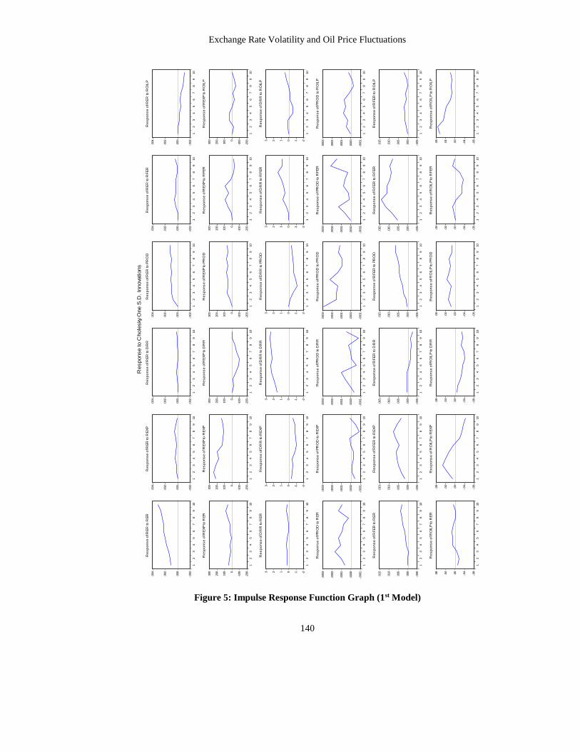
4.4.2Impulse Response Function (IRF) 1st Model Results

IRF tells us about the variation in RER due to one standard deviation change in PROD,

DRR, REXP, RFER and OILP. Some previous studies like Naka & Tufte (1997) and

Ahmed & Wadud (2011) have used this approach to examine the variation. So, graphic

form is stated as below:


140

Figure 5: Impulse Response Function Graph (1st Model)

-.002

.000

.002

.004

12

34

56

78

910

Re

sp

on

se

of R

ER

to R

ER

-.002

.000

.002

.004

12

34

56

78

910

Re

sp

on

se

of R

ER

to R

EX

P

-.002

.000

.002

.004

12

34

56

78

910

Re

sp

on

se

of R

ER

to D

RR

-.002

.000

.002

.004

12

34

56

78

910

Re

sp

on

se

of R

ER

to P

RO

D

-.002

.000

.002

.004

12

34

56

78

910

Re

sp

on

se

of R

ER

to R

FE

R

-.002

.000

.002

.004

12

34

56

78

910

Re

sp

on

se

of R

ER

to R

OIL

P

-200

-1000

100

200

300

12

34

56

78

910

Re

sp

on

se

of R

EX

P to

RE

R

-200

-1000

100

200

300

12

34

56

78

910

Re

sp

on

se

of R

EX

P to

RE

XP

-200

-1000

100

200

300

12

34

56

78

910

Re

sp

on

se

of R

EX

P to

DR

R

-200

-1000

100

200

300

12

34

56

78

910

Re

sp

on

se

of R

EX

P to

PR

OD

-200

-1000

100

200

300

12

34

56

78

910

Re

sp

on

se

of R

EX

P to

RF

ER

-200

-1000

100

200

300

12

34

56

78

910

Re

sp

on

se

of R

EX

P to

RO

ILP

-2-10123

12

34

56

78

910

Re

sp

on

se

of D

RR

to R

ER

-2-10123

12

34

56

78

910

Re

sp

on

se

of D

RR

to R

EX

P

-2-10123

12

34

56

78

910

Re

sp

on

se

of D

RR

to D

RR

-2-10123

12

34

56

78

910

Re

sp

on

se

of D

RR

to P

RO

D

-2-10123

12

34

56

78

910

Re

sp

on

se

of D

RR

to R

FE

R

-2-10123

12

34

56

78

910

Re

sp

on

se

of D

RR

to R

OIL

P

-.0001

.0000

.0001

.0002

.0003

12

34

56

78

910

Re

sp

on

se

of P

RO

D to

RE

R

-.0001

.0000

.0001

.0002

.0003

12

34

56

78

910

Re

sp

on

se

of P

RO

D to

RE

XP

-.0001

.0000

.0001

.0002

.0003

12

34

56

78

910

Re

sp

on

se

of P

RO

D to

DR

R

-.0001

.0000

.0001

.0002

.0003

12

34

56

78

910

Re

sp

on

se

of P

RO

D to

PR

OD

-.0001

.0000

.0001

.0002

.0003

12

34

56

78

910

Re

sp

on

se

of P

RO

D to

RF

ER

-.0001

.0000

.0001

.0002

.0003

12

34

56

78

910

Re

sp

on

se

of P

RO

D to

RO

ILP

-.005

.000

.005

.010

.015

12

34

56

78

910

Re

sp

on

se

of R

FE

R to

RE

R

-.005

.000

.005

.010

.015

12

34

56

78

910

Re

sp

on

se

of R

FE

R to

RE

XP

-.005

.000

.005

.010

.015

12

34

56

78

910

Re

sp

on

se

of R

FE

R to

DR

R

-.005

.000

.005

.010

.015

12

34

56

78

910

Re

sp

on

se

of R

FE

R to

PR

OD

-.005

.000

.005

.010

.015

12

34

56

78

910

Re

sp

on

se

of R

FE

R to

RF

ER

-.005

.000

.005

.010

.015

12

34

56

78

910

Re

sp

on

se

of R

FE

R to

RO

ILP

-.08

-.04

.00

.04

.08

12

34

56

78

910

Re

sp

on

se

of R

OIL

P to

RE

R

-.08

-.04

.00

.04

.08

12

34

56

78

910

Re

sp

on

se

of R

OIL

P to

RE

XP

-.08

-.04

.00

.04

.08

12

34

56

78

910

Re

sp

on

se

of R

OIL

P to

DR

R

-.08

-.04

.00

.04

.08

12

34

56

78

910

Re

sp

on

se

of R

OIL

P to

PR

OD

-.08

-.04

.00

.04

.08

12

34

56

78

910

Re

sp

on

se

of R

OIL

P to

RF

ER

-.08

-.04

.00

.04

.08

12

34

56

78

910

Re

sp

on

se

of R

OIL

P to

RO

ILP

Response to C

hole

sky

One S

.D. In

nova

tions

Ahmed et al.

141

The graph of exchange rate to a unit shock in its own exchange rate is positive throughout

the next ten quarters. It can be seen that positive shocks in real REXP, RFER and PROD

have positive effect on RER, means a positive shock in exports, foreign exchange

reserves and productivity differential lead to appreciation in exchange rate into ten

quarters. The variation of RER to a unit deviation in DRR will be positive from third to

fifth quarter, while other quarters will not show any response to shock. Similarly, the

reaction of RER to positive shock in OILP has negative to overall the selected quarters.

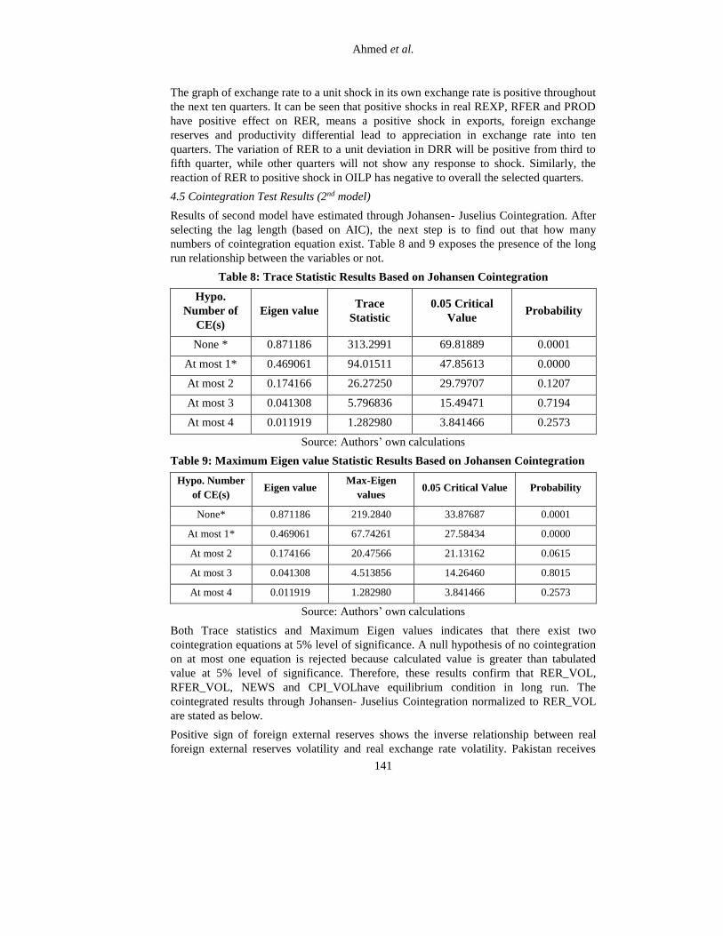
4.5 Cointegration Test Results (2nd model)

Results of second model have estimated through Johansen- Juselius Cointegration. After

selecting the lag length (based on AIC), the next step is to find out that how many

numbers of cointegration equation exist. Table 8 and 9 exposes the presence of the long

run relationship between the variables or not.

Table 8: Trace Statistic Results Based on Johansen Cointegration

Hypo.

Number of

CE(s)

Eigen value Trace

Statistic

0.05 Critical

Value Probability

None * 0.871186 313.2991 69.81889 0.0001

At most 1* 0.469061 94.01511 47.85613 0.0000

At most 2 0.174166 26.27250 29.79707 0.1207

At most 3 0.041308 5.796836 15.49471 0.7194

At most 4 0.011919 1.282980 3.841466 0.2573


Table 9: Maximum Eigen value Statistic Results Based on Johansen Cointegration

Hypo. Number

of CE(s) Eigen value

Max-Eigen

values 0.05 Critical Value Probability

None* 0.871186 219.2840 33.87687 0.0001

At most 1* 0.469061 67.74261 27.58434 0.0000

At most 2 0.174166 20.47566 21.13162 0.0615

At most 3 0.041308 4.513856 14.26460 0.8015

At most 4 0.011919 1.282980 3.841466 0.2573


Both Trace statistics and Maximum Eigen values indicates that there exist two

cointegration equations at 5% level of significance. A null hypothesis of no cointegration

on at most one equation is rejected because calculated value is greater than tabulated

value at 5% level of significance. Therefore, these results confirm that RER_VOL,

RFER_VOL, NEWS and CPI_VOLhave equilibrium condition in long run. The

cointegrated results through Johansen- Juselius Cointegration normalized to RER_VOL

are stated as below.

Positive sign of foreign external reserves shows the inverse relationship between real

foreign external reserves volatility and real exchange rate volatility. Pakistan receives


142

loan, aid and grant from different developed countries that creates fluctuations in

reserves. Moreover, gold and other assets of central bank like bond and certificates are

bought and sold in international and domestic market to fulfill the gap of budget deficit.

This fluctuation in reserves affects exchange rate and make it volatile. This result is

consistent with Hviding (2004).

RER_VOLt= -3.94E-05 +0.047 E-08 RFER_VOLt -1.00 E-06 NEWSt +5.46E-07

CPI_VOLt +0.0055 ROILP_VOLt

T-statistics = [36.9070] [-4.22846] [8.05686] [14.9096]

Positive sign of NEWS showed that actual values of interest rate are less than expected

value. Higher expectation means that investors are more volatile about their decision. So,

this uncertain situation highly effect on exchange rate volatility as results suggested by

Stancik (2006). Results of CPI volatility indicate higher the volatility in CPI, more

volatility will be observed as results reported by Parker, M. (2014). Positive and

significant oil price volatility results show that 1 percent increase in volatility of oil price,

exchange rate leads to volatile about .0055 percent. This result matched with the study of

Selmia et al. (2012), Ogundipe & Ogundipe (2013).

4.5.1 VECM Results

The ECM or speed of adjustment coefficient suggests that these variables converge

towards its long run equilibrium level quarterly in a moderate speed after an oil price

shock. These results were consistent with Aliyu (2009).

Table 10: VECM result of 2nd Model

Variable Coefficient Standard Error T-Statistics

ECT -0.874250 0.31891 -2.74140

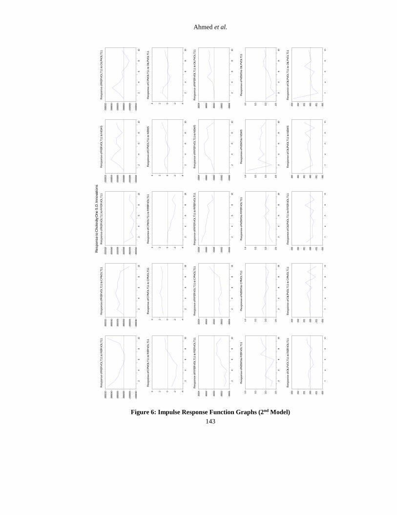
4.5.2 Impulse Response Function (IRF) 2nd Model Results

Graph of real exchange rate volatility to a unit shock in its own volatility is positive up to

six quarter then it becomes negative in seventh quarter to shock. Exchange rate volatility

converts negative to positive after seventh quarter. A positive shock in CPI volatility has

positive effect on real exchange volatility up to ninth quarter but after this quarter, the

positive shock will effect negatively on the volatility of exchange rate. The reaction of

real exchange rate volatility to one standard deviation shock in News and foreign

exchange reserves is negative and positive respectively throughout the tenth quarter.

Shock in real exchange rate volatility has positive on oil price volatility until seven

quarter but after this quarter, this shock has negative impact on oil price volatility.

Ahmed et al.

143

Figure 6: Impulse Response Function Graphs (2nd Model)

-.0000010

-.0000005

.0000000

.0000005

.0000010

.0000015

24

68

10

Response o

f RER

VO

LT11 to

RER

VO

LT11

-.0000010

-.0000005

.0000000

.0000005

.0000010

.0000015

24

68

10

Response o

f RER

VO

LT11 to

CPIV

OLT11

-.0000010

-.0000005

.0000000

.0000005

.0000010

.0000015

24

68

10

Response o

f RER

VO

LT11 to

RFER

VO

LT11

-.0000010

-.0000005

.0000000

.0000005

.0000010

.0000015

24

68

10

Response o

f RER

VO

LT11 to

NEW

S

-.0000010

-.0000005

.0000000

.0000005

.0000010

.0000015

24

68

10

Response o

f RER

VO

LT11 to

OIL

PVO

LT11

-4-2024

24

68

10

Response o

f CPIV

OLT11 to

RER

VO

LT11

-4-2024

24

68

10

Response o

f CPIV

OLT11 to

CPIV

OLT11

-4-2024

24

68

10

Response o

f CPIV

OLT11 to

RFER

VO

LT11

-4-2024

24

68

10

Response o

f CPIV

OLT11 to

NEW

S

-4-2024

24

68

10

Response o

f CPIV

OLT11 to

OIL

PVO

LT1

1

-.00004

-.00002

.00000

.00002

.00004

24

68

10

Response o

f RFER

VO

LT11 to

RER

VO

LT11

-.00004

-.00002

.00000

.00002

.00004

24

68

10

Response o

f RFER

VO

LT11 to

CPIV

OLT11

-.00004

-.00002

.00000

.00002

.00004

24

68

10

Response o

f RFER

VO

LT11 to

RFER

VO

LT11

-.00004

-.00002

.00000

.00002

.00004

24

68

10

Response o

f RFER

VO

LT11 to

NEW

S

-.00004

-.00002

.00000

.00002

.00004

24

68

10

Response o

f RFER

VO

LT11 to

OIL

PVO

LT11

-0.5

0.0

0.5

1.0

24

68

10

Response o

f NEW

S to

RER

VO

LT11

-0.5

0.0

0.5

1.0

24

68

10

Response o

f NEW

S to

CPIV

OLT11

-0.5

0.0

0.5

1.0

24

68

10

Response o

f NEW

S to

RFER

VO

LT11

-0.5

0.0

0.5

1.0

24

68

10

Response o

f NEW

S to

NEW

S

-0.5

0.0

0.5

1.0

24

68

10

Response o

f NEW

S to

OIL

PVO

LT11

-.002

-.001

.000

.001

.002

.003

24

68

10

Response o

f OIL

PVO

LT11 to

RER

VO

LT11

-.002

-.001

.000

.001

.002

.003

24

68

10

Response o

f OIL

PVO

LT11 to

CPIV

OLT1

1

-.002

-.001

.000

.001

.002

.003

24

68

10

Response o

f OIL

PVO

LT11 to

RFER

VO

LT11

-.002

-.001

.000

.001

.002

.003

24

68

10

Response o

f OIL

PVO

LT11 to

NEW

S

-.002

-.001

.000

.001

.002

.003

24

68

10

Respons

e o

f OIL

PVO

LT1

1 to

OIL

PVO

LT1

1

Response to

Chole

sky

One S

.D. I

nnova

tions


144

4.6 OLS Results (3rd Model)

OLS results show that NEWS and POL_REG has not significant impact on real exchange

rate volatility because their t- statistics are insignificant. On the other hand, positive sign

of regime variable investigates that floating exchange rate experience more volatility in

its regime as compare to managed floating exchange rate. Null hypothesis is rejected at

5% level of significance.

RER_VOLt= 1.89E-06-2.18E-07 DNEWSt + 3.12E-06REGt- 8.94E-07 POL_REGt

T-statistics = [-0.454299] [5.755780] [-1.538217]

5. Conclusions

Pakistan experienced too much variation in crude oil prices in last decades. Importance of

crude oil can be recognized from the fact that it uses in all the sectors of the economy.

For this purpose, we focused on crude oil price and their volatilities. This study observes

the impact of oil price volatility on exchange rate fluctuations and finds out the

determinants that affect real exchange rate. For this purpose, we developed three models

by using quarterly data from 1983Q1-2014Q4. This study applied different econometric

techniques to capture the appropriate results. ADF test has used to test the stationarity of

variables because this technique is considered the best technique to examine unit root.

This test confirms that all the variables are integrated in order one. Volatility is measured

through EGARCH (1, 1) as it is considered the best technique that restrains the power of

non-negativity constraint. Lag length of all models is selected through AIC.

Results of EGARCH (1, 1) shows that negative shock in oil price and exchange rate have

larger effect on their volatilities than positive shocks positive. On the other hand,

negative news of foreign exchange reserves and CPI has not any impact on their

volatilities. Based on the finding of Trace and Max Eigen statistics, first model results

show the existence of long run relationship between the variables. Significant results of

productivity differential, oil prices, exports and interest rate differential confirm that

Balassa Samuelson, Dornbusch Model, Obstfeld Rogoff, and un-covered interest rate

parity conditions are applicable in Pakistan. ECM suggests that all the variables in first

model converge towards its long run equilibrium quarterly in moderate speed after an oil

price shock or shock in other explanatory variables as reported by Asari (2011). On the

other hand, second model confirms the results of Selmia et al. (2012) and Ogundipe &

Ogundipe (2013); states that oil price volatility positively effect on exchange rate

volatility. Furthermore, other control variables like real foreign external reserves

volatility, CPI volatility and NEWS also have significant impact on exchange rate

variability. These results are suggested by Hviding (2004), Stancik (2006) and Parker, M.

(2014). Another important finding regarding exchange rate regime is that during the

period of floating exchange rate, exchange rate volatility remains low as compare to

managed floating exchange rate.

IRF results depicted that the reaction of RER to a unit shock in RER is positive on

exports, foreign exchange reserves and productivity differential, while it has a negative

effect on oil price throughout the tenth quarters. Moreover, reaction of real exchange rate

volatility to a unit shock in Real exchange rate volatility, NEWS and CPI volatility have

Ahmed et al.

145

positive while RFER volatility has negatively related to one standard deviation shock in

real exchange rate volatility throughout the tenth quarters.

Pakistan has chosen as an oil importing country; future research can be made on cross

sectional countries by using monthly data or daily data of variables. This study focused

only one oil importing country, so future studies should be extended to oil exporting

countries.

5.1 Policy Implications

Finally, some policy recommendations are drawn on the basis of results. Fluctuations in

oil prices are the major cause for volatility in exchange rate. Government should not give

subsidies on crude oil when oil price goes to decrease because it creates more volatility

that directly hits investor’s decision. Government should take serious steps to improve

market efficiency and make sure that any variability in oil prices is essential and not

negligible. Transparency should be improved in demand side and supply side that will

help us dwindling the volatility of oil prices. Government should make stable economic

policy to keep exchange rate and exchange rate volatility stable. Appreciation is healthier

for a country but in case of Pakistan (where there are so many problems of energy crises

that lowers the level of exports), it has less beneficial. On the other hand, depreciation has

positive impact on a country but it also increase debt burden. Fiscal and monetary policy

can play their role for the stability of exchange rate; fiscal policy can contribute by

keeping away from large and volatile swings in the size of production and exports while

monetary policy can play its role by ensuring that foreign external reserves and interest

rate are stable with domestic price level. The burden of increased oil price should not

shift to the consumers. Government should bear the expensed of increased oil prices itself

in order to keep the domestic demand of oil stable. By ignoring the leverage effect of

foreign exchange reserves volatility and CPI volatility, Government should be worried

about negative shocks in oil price and exchange rate because negative shocks have larger

effect on volatility than positive shock.

REFERENCE

Abrams, R. K. (1980). International Trade Flows Under Flexible Exchange Rates.

Economic Review, 65(3), 3-10.

Adeniyi, O., Omisakin, O., Yaqub, J., & Oyinlola, A. (2012). Oil Price-Exchange Rate

Nexus in Nigeria: Further Evidence from an Oil Exporting Economy. International

Journal of Humanities and Social Science, 2(8), 113-121.

Adubi, A. A., & Okunmadewa, F. (1999). Price, Exchange Rate Volatility and Nigeria's

Agriculture Trade Flows: A Dynamic Analysis. African Economic Research Consortium,

Research Paper,87, 1-35.

Aghion, P., Bacchetta, P., Rancie, R., & Rogoff, K. (2009). Exchange Rate Volatility and

Productivity Growth: The Role of Financial Development. Journal of Monetary

Economics, 56(4), 494–513.

Ahmed, H. J., & Wadud, I. K. (2011). Role of Oil Price Shocks on Macro Economic

Activities: An SVAR Approach to the Malaysian Economy and Monetary Responses.

Energy Policy, 39(12), 8062–8069.


146

Akram, Q. F. (2004). Oil Prices and Exchange Rates: Norwegian Evidence. The

Econometrics Journal, 7(2), 476 -504.

Aliyu, S. U. (2009). Impact of Oil Price Shock and Exchange Rate Volatility on

Economic Growth in Nigeria: An Empirical Investigation. Munich Personal RePEc

Archive, Paper No. 16319.

Asari, F. F., Baharuddin, N. S., Jusoh, N., Mohamad, Z., Shamsudin, N., & Jusoff, K.

(2011). A Vector Error Correction Model (VECM) Approach in Explaining the

Relationship Between Interest Rate and Inflation towards Exchange Rate Volatility in

Malaysia. World Applied Sciences Journal, 12(3), 49-56.

Azid, T., Jamil, M., & Kousar, A. (2005). Impact of Exchange Rate Volatility on Growth

and Economic Performance: A Case Study of Pakistan, 1973–2003. The Pakistan

Development Review, 44(4), 749–775.

Babatunde, M. A. (2015). Oil price shocks and Exchange Rate in Nigeria. International

Journal of Energy Sector Management, 9(1), 2-19.

Bal, D. P., & Rath, B. N. (2015). Nonlinear Causality between Crude Oil Price and

Exchange Rate. Energy Economics, 51, 149- 156.

Basnet, H. C., & Upadhyaya, K. P. (2015). Impact of Oil Price Shocks on Output,

Inflation and the Real Exchange Rate: Evidence from Selected ASEAN Countries.

Applied Economics, 47 (29), 3078-3091.

Berument, M. H., Sahin, A., & Sahin, S. (2014). The Relative Effects of Crude Oil Price

and Exchange Rate on Petroleum product prices: Evidence from a set of Northern

Mediterranean countries. Economic Modelling, 42, 243–249

Cheng , T.-Y., Weng , Y.-C., & Syu, S.-M. (2015). The Asymmetric Causal Relationship

Research of Electricity Price, Exchange Rate and Oil Price-Takes Taiwan Area as an

Example. Journal of Statistics and Management Systems, 18 (5), 463-484.

Calderon, C., & Kubota, M. (2009). Does Higher Openness Cause More Real Exchange

Rate Volatility?Policy Research Working Papers, Paper No. 4896.

Corden, W. M. (1984). Booming Sector and Dutch Disease Economics: Survey and

Consolidation. Oxford Economic Papers, 359-380.

Danmola, R. A. (2013). The Impact of Exchange Rate Volatility on the Macro Economic

Variables in Nigeria. European Scientific Journal, 9(7), 1857- 7431.

Dornbusch, R. (1976). Expectations and Exchange Rate Dynamics. Journal of Political

Economy, 84(6), 1161-1176.

Egert, B. (2002). Estimating the Impact of the Balassa-Samuelson Effect on Inflation and

the Real Exchange Rate during the Transition. Economic Systems, 26(1), 1-16.

Fowowe, B. (2014). Modelling the Oil Price–Exchange Rate Nexus for South Africa.

International Economics, 140, 36–48.

Frenkel, J. A. (1981). Flexible Exchange Rates, Prices, and the Role of " News" : Lessons

from the 1970s. Journal of Political Economy, 89(4), 665-705.

Genc, E. G., & Artar, O. K. (2014). The Effect of Exchange Rates on Exports and

Imports of Emerging Countries. European Scientific Journal, 10(13), 128-141.

Ahmed et al.

147

Government of Pakistan, (2015). Economic Survey of Pakistan 2014 – 15, Federal

Bureau of Statistics, Statistical Division.

Galati, G., & Ho, C. (2001). Macroeconomic News and the Euro/Dollar Exchange Rate.

BIS Working Papers, Paper No. 105.

Hakkio, C. S. (1984). Exchange Rate Volatility and Federal Reserve Policy. Economic

Review (July, Aug.), 18-31, Federal Reserve Bank of Kansas City.

Hau, H. (2002). Real Exchange Rate Volatility and Economic Openness: Theory and

Evidence. Journal of money, Credit and Banking, 34(3), 611-630.

Hilton, M. A. (1984). Effect of Exchange Rate Uncertainity on German and U.S. Trade.

Ferderal Rerserve Bank of New York , 7-16.

Hviding, K., Nowak, M., & Ricci, L. A. (2004). Can Higher Reserves Help Reduce

Exchange Rate Volatility?International Monetary Fund, Paper No. 189.

Izraf, M., & Aziz, A. (2009). Oil Price & Exchange Rate: A Comparative Study between

Net Oil Exporting and Net Oil Importing Countries. In ESDS International Annual

Conference, London.

Jamali, M. B., Shah, A., Soomro, H. J., Shafiq, K., & Shaikh, F.M. (2011). Oil Price

Shocks: A Comparative Study on the Impacts in Purchasing Power in Pakistan. Modern

Applied Science, 5(2), 192- 203.

Javed, Z. H., & Farooq, M. (2009). Economic Growth and Exchange Rate Volatility in

Case of Pakistan. Pakistan Journal of Life and Social Sciences, 7(2), 112-118.

Jhingan, M. (2005). Macroeconomics Theory (10th Edition). Vrinda Publication Ltd,

New-Delhi.

Jhingan, M. L. (2002). Macro Economic Theory Delhi Vrinda Publications (P) Limited.

Delhi Vrinda Publications (P) Limited.

Khan, A. J., & Azim, P. (2013). One-Step-Ahead Forecastability of GARCH (1,1): A

Comparative Analysis of USD- and PKR-Based ExchangeRate Volatilities. The Lahore

Journal of Economics, 18(1), 1–38.

Krugman, P. (1983). Oil Shocks and Exchange Rate Dynamics. In J. A. Frenkel,

Exchange Rates and International Macroeconomics (259-284). University of Chicago

Press.

Li, X., & Jing, Z. (2015). Research on the Trend of Yen Exchange Rate and International

Crude oil Price Fluctuation Around Japan’s Earthquake (Chapter in LISS 2013 -

Proceedings of 3rd International Conference on Logistics, Informatics and Service

Science). Springer Berlin Heidelberg, 915-920.

Manchev, T. (2009). International Foreign Exchange Reserves. Bulgarian National Bank.

Messe, R. F., & Rose, A. K. (1983). Nonlinear, Nonparametric, Nonessential Exchange

Rate Estimation. American Economic Review Papers and Proceedings, 80(2), 603-619.

Mordi, C. N. (2006). Challenges of Exchange Rate Volatility in Economic Management

in Nigeria. Central Bank of Nigeria Bulletin, 30(3). 17-25.


148

Mwangi, S. C., Mbatia, O. L., & Nzuma, J. M. (2014). Effects of Exchange Rate

Volatility on French Beans Exports in Kenya. Journal of Agricultural Economics,

Extension and Rural Development, 1(1), 001-012

Naka, A., & Tufte, D. (1997). Examining impulse response functions in cointegrated

systems. Applied Economics , 29(12), 1593- 1603.

Nelson, D. B. (1991). Conditional Herteroscedasticity in Asset Return: A new Approach.

Econometrica, 59(2), 347-370.

Obadan, M. I. (2006). Overview of Exchange rate Management in Nigeria from 1986 to

date. Central Bank of Nigeria Bulletin, 30(3), 17-25.

Ogundipe, A., & Ogundipe, O. (2013). Oil Price and Exchange Rate Volatility in

Nigeria. Munich Personal RePEc Archive, Paper No. 51668.

Omoniyi, L. G., & Olawale, A. N. (2015). An Application of ARDL Bounds Testing

Procedure to the Estimation of Level Relationship between Exchange Rate, Crude Oil

Price and Inflation Rate in Nigeria. International Journal of Statistics and Applications,

5(2), 81-90.

Parker, M. (2014). Reserve Bank of New Zealand: Bulletin, 77(1), 31-41.

Razi, A., Shafiq, A., Ali, S. A., & Khan, H. (2012). Determinants of Exchange Rate and

its Impact on Pakistani Economy. Global Journal of Management and Business

Research, 12(16), 45-48.

Salisu, A. A., & Mobolaji, H. (2013). Modeling Returns and Volatility Transmission

between Oil Price and US–Nigeria Exchange Rate. Energy Economics, 39, 169–176.

Samara, M. A. (2009). The Determinants of Real Exchange Rate Volatility in the Syrian

Economy. Centre d’Economie de la sarbonne, Universite Paris, 1-36.

Selmia, R., Bouoiyourb, J., & Ayachi, F. (2012). Another look at the Interaction between

Oil Price Uncertainty and Exchange Rate Volatility: The Case of Small Open Economies.

Procedia Economics and Finance , 1, 346-355.

Shaheen, F. (2013). Fluctuations in Exchange Rate and its Impact on Macroeconomic

Performance of Pakistan. Academic Journal, 8(4), 410-418.

Siddqui, R., & Malik, A. (2001). Debt and Economic Growth in South Asia. The

Pakistan Development Review, 40 (4 Part II), 677–688.

Stancik, J. (2006). Determinants of Exchange-Rate Volatility: The Case of the New EU

Members. Charles University, and Center of Economic Research and Graduate Education

[Discussion Paper Series]. Economics Institute of the Academy of Sciences of the Czech

Republic.

nexus between exchange rate volatility and oil price ... between exchange rate volatility and oil...

Documents