http://www.ee.unlv.edu/~b1morris/ee482/

Professor Brendan Morris, SEB 3216, brendan.morris@unlv.edu

EE482: Digital Signal Processing

Applications

Spring 2014

TTh 14:30-15:45 CBC C222

Lecture 11

Adaptive Filtering

14/03/04

Outline

• Random Processes

• Adaptive Filters

• LMS Algorithm

2

Adaptive Filtering

• FIR and IIR filters are designed for linear time-invariant signals

• How can we handle signals when the characteristics are unknown or changing?

• Need ways to update filter coefficients automatically and continually

▫ Track time-varying signals and systems

3

Random Processes

• Real-world signals are time varying and have randomness in nature

▫ E.g. speech, music, noise

• Need to characterize a signal even if full deterministic mathematical definition does not exist

• Random process – sequence of random variables

4

Autocorrelation

• Specifies statistical relationship of signal at different time lags (𝑛 − 𝑘)

▫ 𝑟𝑥𝑥 𝑛, 𝑘 = 𝐸 𝑥 𝑛 , 𝑥 𝑘

▫ Similarity of observations as a function of the time lag between them

• Mathematical tool for detecting signals

▫ Repeating patterns (noise in sinusoid)

▫ Measuring time-delay between signals

Radar, sonar, lidar

▫ Estimation of impulse response

▫ Etc.

5

Wide Sense Stationary (WSS) Process

• Random process statistics do not change with time • Mean independent of time

▫ 𝐸 𝑥 𝑛 = 𝑚𝑥

• Autocorrelation only depends only on time lag

▫ 𝑟𝑥𝑥 𝑘 = 𝐸 𝑥 𝑛 + 𝑘 𝑥 𝑛

• WSS autocorrelation properties ▫ Even function

𝑟𝑥𝑥 −𝑘 = 𝑟𝑥𝑥 𝑘

▫ Bounded by 0 time lag

𝑟𝑥𝑥 𝑘 ≤ 𝑟𝑥𝑥 0 = 𝐸[𝑥2 𝑛 ] Zero mean process: 𝐸 𝑥2 𝑛 = 𝜎𝑥

2

• Cross-correlation

▫ 𝑟𝑥𝑦 𝑘 = 𝐸[𝑥 𝑛 + 𝑘 𝑦 𝑛 ]

6

Expected Value

• Value of random variable “expected” if random variable process repeated infinite number of times

▫ Weighted average of all possible values

• Expectation operator

▫ 𝐸 . = . 𝑓 𝑥 𝑑𝑥∞

−∞

▫ 𝑓(𝑥) – probability density function of random variable 𝑋

7

White Noise

• 𝑣(𝑛) with zero mean and variance 𝜎𝑣2

• Very popular random signal

▫ Typical noise model

• Autocorrelation

▫ 𝑟𝑣𝑣 𝑘 = 𝜎𝑣2𝛿 𝑘

▫ Statistically uncorrelated except at zero time lag

• Power spectrum

▫ 𝑃𝑣𝑣 𝜔 = 𝜎𝑣2, 𝜔 ≤ 𝜋

▫ Uniformly distributed over entire frequency range

8

Example 6.2 • Second-order FIR filter with white noise input

▫ 𝑦 𝑛 = 𝑥 𝑛 + 𝑎𝑥 𝑛 − 1 + 𝑏𝑥 𝑛 − 2 • Mean

▫ 𝐸 𝑦 𝑛 = 𝐸[𝑥 𝑛 + 𝑎𝑥 𝑛 − 1 + 𝑏𝑥 𝑛 − 2 ] ▫ 𝐸 𝑦 𝑛 = 𝐸[𝑥 𝑛 ] + 𝑎𝐸[𝑥 𝑛 − 1 ] + 𝑏𝐸[𝑥 𝑛 − 2 ]

▫ 𝐸 𝑦 𝑛 = 0 + 𝑎 ⋅ 0 + 𝑏 ⋅ 0 = 0 • Autocorrelation

▫ 𝑟𝑦𝑦 𝑘 = 𝐸 𝑦 𝑛 + 𝑘 𝑦 𝑛

▫ 𝑟𝑦𝑦 𝑘 = 𝐸𝑥 𝑛 + 𝑘 + 𝑎𝑥 𝑛 + 𝑘 − 1 + 𝑏𝑥 𝑛 + 𝑘 − 2 ⋅

(𝑥 𝑛 + 𝑎𝑥 𝑛 − 1 + 𝑏𝑥 𝑛 − 2 )

▫ 𝑟𝑦𝑦 𝑘 = 𝐸 𝑥 𝑛 + 𝑘 𝑥 𝑛 + 𝐸 𝑎𝑥 𝑛 + 𝑘 𝑥 𝑛 − 1 + …

▫ 𝑟𝑦𝑦 𝑘 = 𝑟𝑥𝑥 𝑘 + 𝑎𝑟𝑥𝑥 𝑘 − 1 + ⋯

▫ 𝑟𝑦𝑦 𝑘 =

1 + 𝑎2 + 𝑏2 𝜎𝑥2

𝑎 + 𝑎𝑏 𝜎𝑥2

𝑏𝜎𝑥2

0

𝑘 = 0𝑘 = ±1𝑘 = ±2

𝑒𝑙𝑠𝑒

9

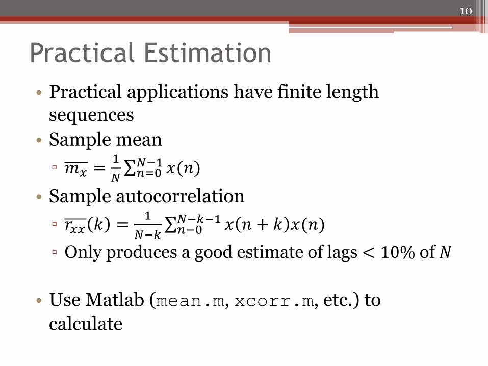
Practical Estimation

• Practical applications have finite length sequences

• Sample mean

▫ 𝑚𝑥 =1

𝑁 𝑥(𝑛)𝑁−1

𝑛=0

• Sample autocorrelation

▫ 𝑟𝑥𝑥 𝑘 =1

𝑁−𝑘 𝑥 𝑛 + 𝑘 𝑥(𝑛)𝑁−𝑘−1

𝑛−0

▫ Only produces a good estimate of lags < 10% of 𝑁

• Use Matlab (mean.m, xcorr.m, etc.) to

calculate

10

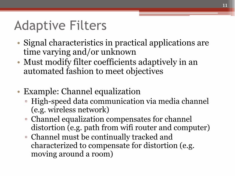
Adaptive Filters

• Signal characteristics in practical applications are time varying and/or unknown

• Must modify filter coefficients adaptively in an automated fashion to meet objectives

• Example: Channel equalization ▫ High-speed data communication via media channel

(e.g. wireless network) ▫ Channel equalization compensates for channel

distortion (e.g. path from wifi router and computer) ▫ Channel must be continually tracked and

characterized to compensate for distortion (e.g. moving around a room)

11

General Adaptive Filter • Two components

▫ Digital filter – defined by coefficients ▫ Adaptive algorithm – automatically update filter

coefficients (weights)

• Adaption occurs by comparing filtered signal 𝑦(𝑛) with a desired (reference) signal 𝑑(𝑛) ▫ Minimize error 𝑒(𝑛) using a cost function (e.g. mean-

square error) ▫ Continually lower error and get 𝑦 𝑛 closer to 𝑑(𝑛)

12

FIR Adaptive Filter

• 𝑦 𝑛 = 𝑤𝑙 𝑛 𝑥(𝑛 − 𝑙)𝐿−1𝑙=0

▫ Notice time-varying weights

• In vector form

▫ 𝑦 𝑛 = 𝒘𝑇 𝑛 𝒙 𝑛 = 𝒙𝑇 𝑛 𝒘 𝑛

▫ 𝒙 𝑛 = 𝑥 𝑛 , 𝑥 𝑛 − 1 , … , 𝑥 𝑛 − 𝐿 + 1 𝑇

▫ 𝒘 𝑛 = 𝑤0 𝑛 , 𝑤1 𝑛 , … , 𝑤𝐿−1 𝑛 𝑇

• Error signal

▫ 𝑒 𝑛 = 𝑑 𝑛 − 𝑦 𝑛 = 𝑑 𝑛 − 𝒘𝑇 𝑛 𝒙 𝑛

13

Performance Function

• Use mean-square error (MSE) cost function

• 𝜉 𝑛 = 𝐸 𝑒2 𝑛

• 𝜉 𝑛 = 𝐸 𝑑2 𝑛 − 2𝒑𝑇𝒘 𝑛 + 𝒘𝑇 𝑛 𝑹𝒘 𝑛

▫ 𝒑 = 𝐸 𝑑 𝑛 𝒙 𝑛 = 𝑟𝑑𝑥 0 , 𝑟𝑑𝑥 1 , … , 𝑟𝑑𝑥 𝐿 − 1 𝑇

▫ 𝑹 – autocorrelation matrix

𝑹 = 𝐸[𝒙 𝑛 𝒙𝑇 𝑛 ]

Toeplitz matrix – symmetric across main diagonal

14

Steepest Descent Optimization • Error function is a quadratic

surface

▫ 𝜉 𝑛 = 𝐸 𝑑2 𝑛 − 2𝒑𝑇𝒘 𝑛 +𝒘𝑇 𝑛 𝑹𝒘 𝑛

• Therefore gradient decent search techniques can be used

▫ Gradient points in direction of greatest change

• Iterative optimization to “step” toward the bottom of error surface

▫ 𝑤 𝑛 + 1 = 𝑤 𝑛 −𝜇

2∇𝜉 𝑛

15

LMS Algorithm • Practical applications do not

have knowledge of 𝑑 𝑛 , 𝑥 𝑛

▫ Cannot directly compute MSE and gradient

▫ Stochastic gradient algorithm

• Use instantaneous squared error to estimate MSE

▫ 𝜉 𝑛 = 𝑒2 𝑛

• Gradient estimate

▫ ∇𝜉 𝑛 = 2 ∇𝑒 𝑛 𝑒 𝑛

𝑒 𝑛 = 𝑑 𝑛 − 𝑤𝑇 𝑛 𝑥(𝑛)

▫ 𝛻𝜉 𝑛 = −2𝑥(𝑛)𝑒 𝑛

• Steepest descent algorithm

▫ 𝑤 𝑛 + 1 = 𝑤 𝑛 + 𝜇𝑥 𝑛 𝑒 𝑛

• LMS Steps

1. Set 𝐿, 𝜇, and 𝒘(0)

▫ 𝐿 – filter length

▫ 𝜇 – step size (small e.g. 0.01)

▫ 𝒘(0) – initial filter weights

2. Compute filter output

▫ 𝑦 𝑛 = 𝒘𝑇 𝑛 𝒙 𝑛

3. Compute error signal

▫ 𝑒 𝑛 = 𝑑 𝑛 − 𝑦 𝑛

4. Update weight vector ▫ 𝑤𝑙 𝑛 + 1 = 𝑤𝑙 𝑛 + 𝜇𝑥 𝑛 − 𝑙 𝑒 𝑛 ,

𝑙 = 0,1, … 𝐿 − 1

• Notice this requires a reference signal

16