EE 364B: Wind Farm Layout Optimization viaSequential Convex Programming

Jinkyoo Park

1 Introduction

In a wind farm, the wakes formed by upstream wind turbines decrease the power outputsof downstream wind turbines by reducing wind speed. This wake interference significantlylowers the power production of a wind farm, especially that of a large-scale wind farm. Inthis paper, we express wind farm power as a differentiable function of location variables.We then apply a sequential convex programming (SCP) to optimize the locations of a largenumber of wind turbines to maximize the wind farm power.

2 Background

2.1 Wake model

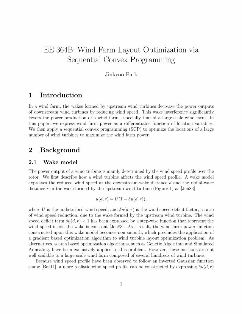
The power output of a wind turbine is mainly determined by the wind speed profile over therotor. We first describe how a wind turbine affects the wind speed profile. A wake modelexpresses the reduced wind speed at the downstream-wake distance d and the radial-wakedistance r in the wake formed by the upstream wind turbine (Figure 1) as [Jen83]

u(d, r) = U(1− δu(d, r)),

where U is the undisturbed wind speed, and δu(d, r) is the wind speed deficit factor, a ratioof wind speed reduction, due to the wake formed by the upstream wind turbine. The windspeed deficit term δu(d, r) < 1 has been expressed by a step-wise function that represent thewind speed inside the wake is constant [Jen83]. As a result, the wind farm power functionconstructed upon this wake model becomes non smooth, which precludes the application ofa gradient based optimization algorithm to wind turbine layout optimization problem. Asalternatives, search based optimization algorithms, such as Genetic Algorithm and SimulatedAnnealing, have been exclusively applied to this problem. However, these methods are notwell scalable to a large scale wind farm composed of several hundreds of wind turbines.

Because wind speed profile have been observed to follow an inverted Gaussian functionshape [Bar11], a more realistic wind speed profile can be constructed by expressing δu(d, r)

1

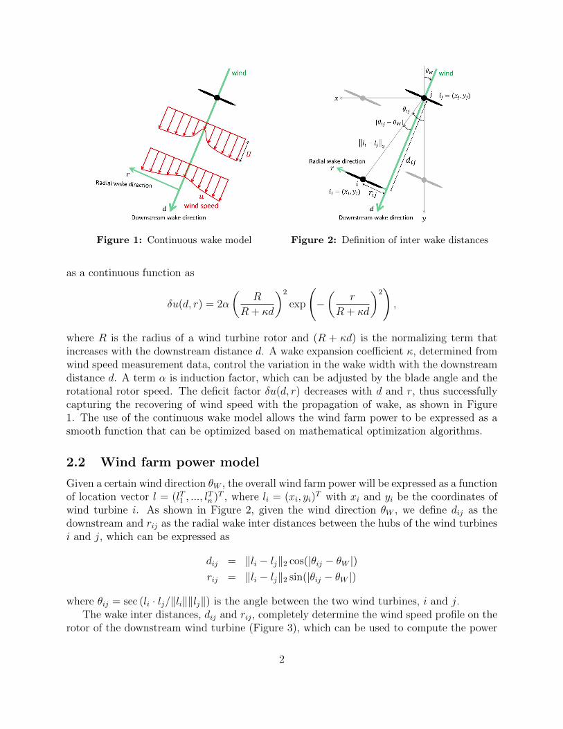
Figure 1: Continuous wake model Figure 2: Definition of inter wake distances

as a continuous function as

δu(d, r) = 2α

(R

R + κd

)2

exp

(−(

r

R + κd

)2),

where R is the radius of a wind turbine rotor and (R + κd) is the normalizing term thatincreases with the downstream distance d. A wake expansion coefficient κ, determined fromwind speed measurement data, control the variation in the wake width with the downstreamdistance d. A term α is induction factor, which can be adjusted by the blade angle and therotational rotor speed. The deficit factor δu(d, r) decreases with d and r, thus successfullycapturing the recovering of wind speed with the propagation of wake, as shown in Figure1. The use of the continuous wake model allows the wind farm power to be expressed as asmooth function that can be optimized based on mathematical optimization algorithms.

2.2 Wind farm power model

Given a certain wind direction θW , the overall wind farm power will be expressed as a functionof location vector l = (lT1 , ..., l

Tn )T , where li = (xi, yi)

T with xi and yi be the coordinates ofwind turbine i. As shown in Figure 2, given the wind direction θW , we define dij as thedownstream and rij as the radial wake inter distances between the hubs of the wind turbinesi and j, which can be expressed as

dij = ‖li − lj‖2 cos(|θij − θW |)rij = ‖li − lj‖2 sin(|θij − θW |)

where θij = sec (li · lj/‖li‖‖lj‖) is the angle between the two wind turbines, i and j.The wake inter distances, dij and rij, completely determine the wind speed profile on the

rotor of the downstream wind turbine (Figure 3), which can be used to compute the power

2

output of the wind turbine. Based on the conservation momentum, the averaged wind speeduij on the rotor of wind turbine i (whose rotor area is πR2) due to the wake by wind turbinej can be computed as

uij(li, lj, θW ) = (1/πR2)

∫Aij

u(d, r)dA =

∫Aij

U(1− δu(d, r))dAij

where Aij, determined by dij and rij, defines the region on the rotor of the downstream windturbine i upon which the wind flow energy is integrated. Then, the averaged deficit factorδuij can be calculated from uij = U(1− δuij), which will be used to aggregate the influencesof multiple wakes.

Figure 3: 3D view of wake expansion Figure 4: Influences of multiple wake

In a wind farm, multiple wakes formed by upstream wind turbines concurrently affectthe power production of a downstream wind turbine (Figure 4). To account for the wakes bymultiple wind turbines, based on the conservation of kinetic energy for deficit wind speed,the aggregated deficit term δui(l, θW ) is expressed as [KHJ86]:

δui(l, θW ) =

√∑N

j=1,j 6=i(δuij(li, lj, θW ))2.

The averaged wind speed for wind turbine i influenced by wakes by all the wind turbines ina wind farm then can be expressed as

ui(l, θW ) = U(1− δui(l, θW )).

Accordingly, the power of wind turbine i can be expressed as a (smooth) function of thelocation vector l and the wind direction θW as

Pi(l, θW ) = (1/2)ρACP (ui(l, θW ))3 = (1/2)ρACP

(U

(1−

√∑N

j=1,j 6=i(δuij(li, lj, θW ))2

))3

,

where ρ is the air density and CP is the power coefficient representing the efficiency of theenergy conversion from wind flow to mechanical energy.

3

3 Optimal wind farm layout problem

The optimal wind farm layout problem is to determine the locations of wind turbines thatmaximize the expected wind farm power production, which can be formulated as

maximize f(l) := E[∑N

i=1 Pi(l, θW )]

subject to ‖li − lj‖2 ≥ 4D for i, j = 1, ..., N, i 6= jl � l � l,

(1)

where the expectation is taken over the distribution of the wind speed θW . The expectedwind farm power function can be approximated as a sum over a discrete sample with the wind

direction probability mass function Pr(θW,k), i.e., f(l) =∑K

k=1 Pr(θW,k)(∑N

i=1 Pi(l, θW,k))

.

The optimization variable l = (lT1 , ..., lTn )T with li = (xi, yi)

T should satisfy the twoconstraints. First, the inter-distance between every pair or two wind turbines should belarger than a certain limit (we set four times the rotor diameter D) for the safe operation.Second, each wind turbine is allowed to be located in a certain region, which is incorporatedin the location limit vectors l and l. The various shapes of wind farm sites can be imposedby manipulating individual components in the vectors l and l.

4 Sequential convex programming

Figure 5: Convexified feasible region for wind turbine i

The derived expected wind farm power function f(l) is not concave and the constraintson the minimum inter distance is not convex, which makes it difficult to apply conventionalconvex programming to (1). To solve Eq. (1), we apply sequential convex programming(SCP) to solve the approximated convex programming iteratively until it reaches a localoptimum. Using the analytically evaluated gradient∇f

(l(k)), and the approximated Hessian

B(k) based on the damped BFGS update [NW00] at the current estimate l(k), the SCPapproximates (1) into

minimize f(l(k))

+∇f(l(k))T (

l − l(k))

+ (1/2)(l − l(k)

)TB(k)

(l − l(k)

)subject to

(l(k)i − l

(k)j

)T(li − lj) ≥ 4D‖l(k)i − l

(k)j ‖2 for i, j = 1, ..., N, i 6= j

l � l � ll ∈ T (k),

(2)

4

which can be efficiently solved by CVX [GB13]. Note that the objective function is approx-imated as a quadratic function and the minimum inter-distance constrains are linearized(Figure 5). The solution of (2) will be used as the next iteration point l(k+1) providing thatthe ratio between the increase in the true function value and the increase in the approxi-mated function value is larger than a certain limit. The constrain l ∈ T (k), referred to as atrust region, is additionally imposed to guarantee that the approximated function is close tothe true function; the approximation is close to the true objective function only around thecurrent estimate l(k). Based on the solution of (2), the trust region T (k) = {l||l− l(k)| < ρ(k)}is also adjusted to guarantee the convergence to a local optimum. The overall algorithm isdescribed in Algorithm 1.

Algorithm 1 Wind farm layout optimization using SCP

1: initialize (choose) l(0)

2: initialize the trust region T (0) = {l||l− l(0)| < ρ(0)}3: while

∥∥l(k) − l(k)∥∥2< ε do

4: Find the solution l by solving Equation (2)

5: iff(l(k))−f(l)

f(l(k))−f(l)≥ α then

6: update the solution l(k+1) = l7: increase the trust region ρ(k+1) = βsuccρ(k)

8: else9: reject the current solution l(k+1) = l(k)

10: decrease trust region ρ(k+1) = βfailρ(k)

11: end if12: increment k ← k + 113: end while

5 Numerical Simulation

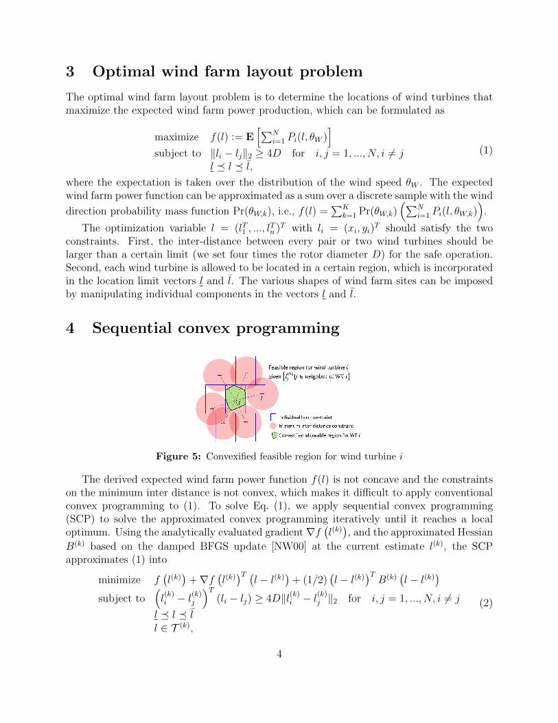
To illustrate the proposed approach, we optimize the locations of 100 wind turbines on atarget site (Figure 6) with the annual wind speed distribution (Figure 7).

(a) Target wind farm site (b) Annual wind direction distribution

Figure 6: Illustration of wind farm layout design (figure from www.windfinder.com)

Figure 7 compares the improvement of wind farm power efficiencies, a ratio of total windfarm power to the maximum wind farm power with no wake interference, with iterations ofSCP starting from 10 different initial locations. Each of initial point is randomly disturbedone from the locations determined by the traditional design approach arraying wind turbinesin a staggered grid pattern. We use different strategies of imposing box constraints on windturbines: (a) global box constraint imposing every wind turbines to be located in a big

5

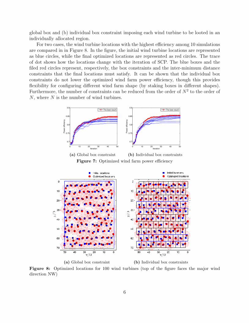
global box and (b) individual box constraint imposing each wind turbine to be looted in anindividually allocated region.

For two cases, the wind turbine locations with the highest efficiency among 10 simulationsare compared in in Figure 8. In the figure, the initial wind turbine locations are representedas blue circles, while the final optimized locations are represented as red circles. The traceof dot shows how the locations change with the iteration of SCP. The blue boxes and thefiled red circles represent, respectively, the box constraints and the inter-minimum distanceconstraints that the final locations must satisfy. It can be shown that the individual boxconstraints do not lower the optimized wind farm power efficiency, though this providesflexibility for configuring different wind farm shape (by staking boxes in different shapes).Furthermore, the number of constraints can be reduced from the order of N2 to the order ofN , where N is the number of wind turbines.

0 10 20 30 40 50

0.7

0.75

0.8

0.85

0.9

Iteration

Po

we

r e

ffic

ien

cy

The best result

(a) Global box constraint

0 10 20 30 40 50

0.7

0.75

0.8

0.85

0.9

Iteration

Po

we

r e

ffic

ien

cy

The best result

(b) Individual box constraints

Figure 7: Optimized wind farm power efficiency

(a) Global box constraint (b) Individual box constraints

Figure 8: Optimized locations for 100 wind turbines (top of the figure faces the major winddirection NW)

6

References

[Bar11] J. Bartl. Wake Measurement Behind an Array of Two Model Wind Turbines. M.S.Thesis, Royal Institute of Technology, Stockholm, 2011.

[BV04] S. Boyd and L. Vandenberghe. Convex Optimization. Cambridge University Press,2004.

[GB13] M. Grant and S. Boyd. The CVX User’s Guide 2.0. CVX Research, INC., 2013.

[Jen83] N. Jensen. Tech. Rep 2411: A Note on Wind Generator Interaction. Riso NationalLaboratory, 1983.

[KHJ86] I. Katic, J. Hojstrup, and N. Jensen. A simple model for cluster efficiency. WindEnergy Association Conference and Exhibition, 12:109–138, 1986.

[NW00] J. Nocedal and S. Wright. Numerical Optimization. Springer, 2000.

7