econometric analysis, 5th edition - agricultural & applied economics

Printing Date Page Erratum http://pages.stern.nyu.edu/~wgreene/Text/Errata/ERRATA5.htm

1 of 25 11/17/2006 9:20 AM

Econometric Analysis, 5th Edition

ERRATA and DISCUSSION Last updated September 5, 2006

/

Page Number

Date Posted

Errata

PAGENUMBER

DATE erratum ... may be repeated for more than one on the page

xxx 12/15/02 In the acknowledgements: Badi Baltagi has moved from Houston to Texas A&M. FrankChaloupka has moved from CUNY to University of Illinois at Chicago. Update (September2005), Professor Baltagi has moved to Syracuse University.

3 9/30/03 Alan Mehlenbacher notes that Figure 1.1 is not drawn quite accurately with the actual data.The picture looks slightly different if drawn, e.g., with Excel or another econometrics package.The main observable difference will be that the two residuals for the points at the upperrightmost in the figure are actually positive, though the figure shows them negative. (Alan Mehlenbacher, Expert Decision Software.)

12 1/6/03 In the gasoline demand model in Example 2.3, "income" should be "income/pop" (Dr. Maurizio Zanarti, University of Glasgow.)

20 8/10/03 In the third line from the bottom, in the last term in the expression for S( b0 ), the first b0should be b0 '. (Alan Mehlenbacher, Expert Decision Software.)

23 11/15/04 In the third line of the paragraph above Theorem 3.1, "regression of G on T" should be"regression of T on G." (Hai-Anh H. Dang, University of Minnesota.)

25 03/11/06 In the line after the second equation on the page, in "As a consequence of (3-15) and (3-16)..."the (3-15) should be (3-14) (Chwen-Chi Liu, Feng Chia University, Taiwan.)

36 11/26/04 In the final equation on the page, in the expression for R2, the numerator should be b'X'M0y.(Hai-Anh Dang, University of Minnesota.)

47 6/23/05 In the first line of the page, "is the transpose" should be "is the inverse" (Mr.Chanyoung Eom .)

50 4/6/04 In footnote 1, B10.3 should be B11.4. (Mr. Spanos Andreas, University of Exeter.)

50 6/29/04 It should be noted that the derivation leading to (4-13) and (4-14) is conditional on X. (Harald Badinger, European Institute, Vienna.)

53 6/23/05 If one extracts the data from Table F2.2 and computes the regression model shown at the topof the page, the constant term will be -12.341. The value -7.737 shown there results frommultiplying the dependent variable by 100 before taking (base e) logs. (William Greene, New York University.)


2 of 25 11/17/2006 9:20 AM

53 07/08/03 At the end of Example 4.4, the 95% critical value for the t distribution given there, 2.04, is fora two tailed test. Since the test is one tailed, the critical value should be 1.695, instead. (Tom Doan, Estima, Inc.) .

56-57 12/31/04 The variances in (4-16) and (4-18) should be conditioned on X. (Hai-Anh Dang, University of Minnesota)

58 02/17/05 In Table 4.4, the variance inflation factor for YEAR should be 143.4638, not 251.839.(Giuseppe Vittucci, Italy.)

59 12/31/04 The result given in the third line, E[d]=δ= CLCL'β is not correct. The principal componentswould normally be defined for orthonormalized variables, which would make it difficult towrite Z out as a simple linear combination of the columns of X. However, if we do not centeror normalize the data first (suppose they are already standardized), then the columns of CLwould be the characteristic vectors of X'X corresponding to the L largest characteristic roots, which we can array in the LxL diagonal matrix ΛL and by the definition, X'XCL = CLΛL. In

this case, (Z'Z)-1 would equal (CL'X'XCL)-1= ΛL-1. Then Z'y= CL'X'(Xβ+ ε)= CL'X'Xβ+

CL'X' ε Combining terms, (Z'Z)-1Z'y= ΛL-1 ΛL CL'β + ΛL

-1CL'X'ε. Taking expectationsleaves E[d]=δ=CL'β. (Hai-Anh Dang, University of Minnesota and William Greene, New York University )

60 6/26/03 In the 12th line on the page, there should be a period to end the sentence before the word "Last." (Erhan Uluceviz from Bogazici University, Istanbul/Turkey.)

63 7/18/03 In the second line of exercise 4, exp(-λεi) should be exp(-εi/λ). (Seher Fazlioglu, Bogazici University, Istanbul, Turkey)

73 11/26/04 Two lines up from the end of the page, in the item xt+r, since r has not been defined earlier, it might be noted that r should be greater than 0. (Hai-Anh Dang, University of Minnesota.)

76 11/26/04 In the second sentence after assumption A19, the term zi should be zi. (Hai-Anh Dang, University of Minnesota.)

77 3/11/03 In the statement of Theorem 5.3, Assumptions AS5 and AS5a should be A5 and A5a. (Paul Glewwe, University of Minnesota.)

78 3/11/03 In the sentence after 5-22, it should be noted that substituting X^ into (5-21) does not simplifyto that result unless Z and X have the same number of columns. In the more usual case inwhich Z has more columns than X, the asymptotic covariance matrix will be based on theinverse of the matrix in brackets in (5-22) instead, as Z'X will not be square and will not beinvertible. (Paul Glewwe, University of Minnesota.)

82 10/3/03 Just above the third equation on the page, the reference to A.7.12 should be to A.6.12. (Darren K Hayunga, Louisiana State University).

83 3/12/03 In Example 5.3, the results claimed in the example are not actually based on the disposablereal personal income suggested in the text; they are based on real GDP instead. The data forthe example are on the website for the text. They can be downloaded by going tohttp://www.stern.nyu.edu/~wgreene and following the links to "Publications" then to thetextbook (first on the list) then to data table 5.1. Also, the suggestion is made in the example tobase the OLS estimates on the full 204 observations and the IV results on 203 observationsomitting the first. The difference will be minor, but in the interest of consistency (Thorownotwithstanding), we'll do the whole thing with 203 observations. The correct results can be


3 of 25 11/17/2006 9:20 AM

produced with the following LIMDEP code. Stata, TSP, SAS or EViews users will have theirown version:

sample;1-204$create;ct1=realcons[-1];yt1=realdpi[-1]$create;ct=realcons;yt=realdpi$namelist;x=one,yt$namelist;z=one,yt1,ct1$sample;2-204$regress;lhs=ct;rhs=x$calc;s2=ssqrd$matrix;bls=b$regress;lhs=yt;rhs=z;keep=yth$namelist;xh=one,yth$2sls;lhs=ct;rhs=x;inst=z$matrix;biv=b$matrix;list;d=biv-bls$matrix;vd=s2*-s2*$matrix;list; h523=d'*mpnv(vd)*d $regress;lhs=ct;rhs=x,yth$

The results are H=8.48139 for (5-23) and a t statistic of 2.968, or an F statistic of 8.809 for(5-24). (Michael Plotzke, Department of Economics, Washington University pointed out thediscrepancy and noted the identity of the variable that produced the results given in the text.)

87 9/15/05 In the fifth equation on the page, α1/α2 in the first term and v/α2 in the last term should bemultiplied by β4. (Dr Juan Paez-Farrell, Cardiff Business School, Cardiff, Wales).

89 5/26/04 In the discussion of the measurement error problem, in the equation yij = βSij + εij, it shouldbe noted that Sij is assumed to have a zero mean, so that the various moments in the nextequation are variances not just expected squares. (Harald Badinger, European Institute, Vienna).

92 9/19/05 In the Chuchy-Schwartz inequality, Schwartz should be Schwarz. This name is also misspelledat several other points in the text and, apparently, at many points in many other texts as well.(Christian Kleiber, University of Dortmund, Germany

96 4/23/04 In footnote 2, B.10.5 should be B.11.6. (Jin John Lei, Department of Economics, Simon Fraser University and Ramiro A. Málaga Ortega, Departamento de Economía,Pontificia UniversidadCatólica del Perú.

96 6/29/04 As on page 50 with the t statistic, it should be noted that the chi-squared statistic on page 96and the derivation leading to the F statistic on page 97 is conditional on X. (Harald Badinger, European Institute, Vienna.)

97 10/10/05 After (6-7) the definition of >b>R does not define what is in the other elements of the singlerow in R other than the one in the jth position. It should be noted that R is a row of K zeros save for the one in the jth position. (Georgios Stergianopoulos, Department of Economics, University of Toronto).

99 12/31/04 At the end of Example 6.1, the denominator degrees of freedom for the F statistic should be198, not 199. (Hai-Anh Dang, University of Minnesota)

103 5/11/05 In Table 6.2, some numerical errors: (1) In column 2, Cobb-Douglas, 0.18840 should be 0.18837; (2) In the center panel, in the first column, 3.61363 should be 3.61364 and -0.96406should be -0.96405; (3) In the final colunmn of the center panel, 3.583 should be 3.582. (4) In


4 of 25 11/17/2006 9:20 AM

the first column of the bottom panel, 0.00189 should be 0.001189 and 0.2332 should be-0.2332. (Professor Randy Campbell, Economics, Mississippi State University)

104 5/11/05 In line 4, 1.8891 should be 1.8991. 8 lines below the equations for lnY, 9.375 should be 9.935.In the next line, 0.94339 should be 0.92006. (Professor Randy Campbell, Economics, Mississippi State University)

104 12/31/04 In the first line of the page, "critical value given earlier" should be "95% critical value of 4.26.Three lines later, the value of 3.49 should be 3.47. (Hai-Anh Dang, University of Minnesota)

105 6/29/04 Five lines up from the last equation on the page, the "See Theorem 4.4 and (4-13)" should nowstate "See Theorem 4.4, Section 4.7.5 and (4-13)." (Harald Badinger, European Institute, Vienna.)

107 6/29/04 In the presentation of Theorem 6.1, after (3), D.21 should be D.16. (Harald Badinger, European Institute, Vienna.)

107 1/6/05 In the proof of Theorem 6.1, it might be noted that P is assumed to be positive definite andsymmetric, though both are implied by the earlier assumptions about R (full row rank) and Q(positive definite). The sentence "Let T be the inverse square root of P." is actually reduntant,

since T = P-1 is stated earlier. In the paragraph that follows the proof, "G.4" and "G.5" shouldbe "G.3" and "G.4," respectively. (Hai-Anh Dang, Unviversity of Minnesota.)

109 6/29/04 Four lines below (6-26), "D.2.2" should be "D.22." (Harald Badinger, European Institute, Vienna.)

109-110 5/15/03 In the calculations for Example 6.3, the wrong value is being used for Asy.Cov[b,c]. The-0.0003298 should be -0.0008207. Make this change in the text 7 lines up from the bottom andin the last line of the page. The result 0.17192 should then be 0.0002585. On the next page, inthe top line, 0.41464 should now be 0.016078. Making this change in the computation of zproduces -0.37131. In the third line of the second paragraph, again change 0.0003298 to0.0008207. The 0.03136 should now be sqr(0.000001401) = 0.00118 and the t ratio should now be -0.38135 rather than -0.01435. The inference is the same as before. The remainder ofthe discussion can remain unchanged. (Professor Noel Roy, Department of Economics,Memorial University of Newfoundland, Canada.)

110 1/6/05 In the first line of text after equation (6-28), G should have a "^" above it. (Hai-Anh Dang, Unviversity of Minnesota.)

119 11/14/02 In the regression results given in the middle of the page, the constant term, 13.56, should be 13.23. This "correction" posted 11/14/02, is erroneous. The value 13.56 given in the text is correct. (Giuseppe Vittucci, Italy.Table 7.2 is correct as given in the text, but it is a bit confusing. The F tests are against thehypotheses that the blocks of dummy variable coefficients are zero. Thus, in the "Time Effects" regression, where the sum of squares is shown to be 1.03470, this sum of squaresoccurs in a model which contains only the time dummies and not the firm dummies. Thus, 5restrictions are imposed. Hence, the F test has 5 numerator degrees of freedom, now the 14that might appear to be the case. Likewise, the Firm Effects model arises by imposing 14restrictions on the Full model.

123 2/17/05 Two lines up from equation (7-6), sy/sk should be sk/sy. (Giuseppe Vittucci, Italy)


5 of 25 11/17/2006 9:20 AM

126 9/26/05 In the first line of Table 7.3, the value of R2 should be 0.932 not 0.942. (Juan Paez-Farrell, Cardiff Business School)

133 12/23/05 In line 7 of Section 7.4.4, in "...probability of a type I error will be smaller...," "smaller" shouldbe "larger." (Patrick Eugster, Socioeconomic Institute, Zürich, Switzerland.)

134 7/07/03 In the second equation at the beginning of Section 7.5.1, the "n" in the denominator inside thelarge parentheses should be a "T." (Zhaohui Han, Department of Economics, IndianaUniversity.)

140 7/30/03 In the equation at the bottom of page 140, the matrix V1 should be qualified by a (π). (Tom Doan, Estima.)

141 7/30/03 In the definition of the LM statistic in the middle of the page, the Vs in the equation should allbe Ws. (Tom Doan, Estima.)

143 11/14/02 In Table 7.2, The LM and LR row labels are interchanged. The first row should be labeled LRand the third LM. (Saeed Moshiri, Department of Economics, Memorial University of Newfoundland.)

143 9/9/04 In Table 7.2, the two values 4.22 and 6.07 must be interchanged. (Dr. Thomas Stark, Federal Reserve Bank, Philadelphia.)

149 1/6/05 At the end of the first paragraph of Example 8.1, it might be noted that in assuming that γ is positive, we are assuming that the good in question is a normal good. It would be negative foran inferior good, though, of course, this is unlikely for gasoline. (Hai-Anh Dang, Unviversity of Minnesota.)

154 1/27/05 In Section 8.3.2, the tests described in the two paragraphs are identical. The discussionsuggests, incorrectly, otherwise. (Paul Glewwe, University of Minnesota.)

169 3/08/05 In Theorem 9.2, the reference to (9-3) should be to (9-9) (Giuseppe Vittucci.)

177 11/28/05 In example 9.7, in the first numerical example, the critical value should be 3.84, not 4.18.(Jin Lei, Department of Economics, Northern Illinois University.)

178 11/20/03 In the last equation on the page, the β after the H-hat should also have a hat on it. ( Jia Li, China Center for Economic Reserch, Peking University, Beijing, China .)

180 11/20/03 In table 9.2, in the test results for the PE tests, in the first row, the three values should be209.354 (26.758), 7.821, respectively. For the second test, the results should be -0.00004188(0.0002613), -0.160, respectively. ( Jia Li, China Center for Economic Research, Peking University, Beijing, China .)

182 3/08/05 In the second line after the third equation on the page, 9.5.1 should be 5.4. (Giuseppe Vittucci.)

183 6/18/04 In the second paragraph of Example 9.9, it is stated that the MPC is βYγ-1. It should be βγYγ-1.Making this correction in the computation changes the reported value from 0.8567 to 1.1543.(The reported standard error is correct.) (Mr. Luis Roberto Inui, Brazil..)


6 of 25 11/17/2006 9:20 AM

185 12/25/04 There is a minor inconsistency between the presentations of the Murphy and Topel result onpage 185 and on 510 resulting from the scaling by n of the matrices R, C, Vc and Vb (whichcorrespond to V1 and V2). For them to be fully consistent, on page 185, remove the n before“plim” in the definitions of R and C, define Vb as n times the asymptotic variance matrix of β^, Vc as n times the asymptotic covariance matrix of γ^, and in the expression at the bottomof page 194, divide the entire assemblage by n. (As they stand, the two statements provide thesame answer.)

188 01/07/06 In Table 9.4, in the results for Step 2, the first column of standard errors should be denoted"St.Er." not "St.Er.*" (Dr. Harald Badinger,Europainstitut, Wirtschaftsuniversitat Wein (Europe Institute, Vienna University of Economics and Business Administration).) Also in thistable, the coefficient on AGE should be -0.07328, not -0.7328 (Marc Tanguay, Statistics Canada).

199 11/10/03 In the first unnumbered equation on the page, there is a stray equals sign after "plim." "Plim="should be just "Plim." (Paul Glewwe, University of Minnesota.)

201 7/7/05 In the equation above (10-17), there is a stray comma that should be deleted before the closingsquare bracket. (Wim Gielis, University of Antwerp, Belgium.)

203 11/15/04 In the first line of Assumption GMM1, "The population moment converges ..." should be "Thesample moment converges..." (Randall S. Romero Aguilar, Banco Central de Costa Rica.)

203 7/7/05 In the 5th line of Assumption GMM2, the "K" should not be bold. (Wim Gielis, University of Antwerp, Belgium.)

206 4/28/05 In the last line of Theorem 10.6, inside the square brackets, the matrix V-hat should be

V-hat-1. (Wim Gielis, University of Antwerp, Belgium.)

221 12/15/02 In Table 11.1, the standard error for the constant in the first column for D. and M. (1) shouldbe 220.79, not 270.79. The mean expenditure reported there, $189.02, applies to the full 100observations. The correct value for the 72 observations used in the regression is $262.53.(Steve Olley, National Economic Research Associates.)

225 10/24/05 In the definition of the matrix PX in the equation before (11-13), the vectors x1, x1 and xnshould all be transposed. (Prof. Toshihiro Uchida, Department of Economics, University of the West Indies, Mona .)

230 11/15/04 In the large 3x3 bracketed matrix expression near the bottom of the page, the g' at the 3,2 element should not have a prime, but the g at the 2,3 element should have a prime (and doesnot in the text). (Hai-Anh H. Dang, University of Minnesota.)

231 11/15/04 In the large matrix expression at the top of the page, the leftmost term in the curled bracketsshould have a prime - that is, be transposed). Equivalently, in the left set of curled brackets, gshould be g'. (Hai-Anh H. Dang, University of Minnesota.)

231 7/30/03 In Table 11.2, in the leftmost column with the model descriptions, in the 4th model, the zi

should be (1,Ii,Ii2). (Tom Doan, Estima.)

231 9/8/04 Line 6. Bruesch should be Breusch. (Dr. Harald Badinger,Europainstitut, Wirtschaftsuniversitat Wein (Europe Institute, Vienna University of Economics and BusinessAdministration).)


7 of 25 11/17/2006 9:20 AM

233 9/8/04 In the last line of the page, H should have an overbar to be consistent with the definition onpage 939 (E-23). (Dr. Harald Badinger,Europainstitut, Wirtschaftsuniversitat Wein (Europe Institute, Vienna University of Economics and Business Administration).)

245 7/30/03 In example 11.8, in the regression of squared residuals on a constant and 10 lagged values, the

R2 should be 0.09795 and the chi-squared statistic is 1964*0.09795 = 460.378. Theconclusions are the same. (Tom Doan, Estima.) (This is the erratum posted in 7/30/03.Christian Kleiber, University of Dortmund, points out that 1964*0.09795 equals 192.4, not460.378. 9/19/05.)

251 9/8/04 In the discussion of Example 12.3, it might be noted that there is a third source of serial correlation (besides model misspecification or being an anticipated part of the model): datatransformations that are carried out purely for the puropse of estimation, e.g. first differencingin dynamic panels to eliminate the individual effects. (Dr. Harald Badinger,Europainstitut, Wirtschaftsuniversitat Wein (Europe Institute, Vienna University of Economics and BusinessAdministration).)

254 7/31/05 In the second to last equation, in Var[εt] = σ2, there should be a subscript; Var[εt] = σε2. (Wim

Gielis, University of Antwerp, Belgium.)

256-257 11/1/02 Expectations and variances of ut should be conditioned on X. Since the text does state (at thetop of page 257) that ut is white noise, this is in fact, implied.Text does not emphasize that the diagonal elements of OMEGA and R are both equal to one

and that OMEGA = R. Also that sigma2OMEGA = gamma0R. (Paul Glewwe, University of Minnesota.)

261-263 11/1/02 Theorems 12.1 and 12.2 specify that the time series zt is stationary, but it is unclear whetherweak or strong stationarity is needed. The use of the word "stationary" by itself suggests thatstrong stationarity is being assumed (as in Definition 12.1), but the comment on the top of p.261 that econometricians always try to "dispense with unnecessary assumptions" suggests thatweak stationarity is implied." Page 261 notwithstanding, the theorems require strongstationarity.In the definition of ergodicity, in the equation given there, there is a missing "]" at the end ofthe first line and a missing "]" in the middle of the second line. At the beginning of thedefinition, zt should be italic, not bold.The assumption that the time series process zt is stationary implies that E[zt] is finite, so why mention this in the theorem as if it were an additional assumption? Also, doesn't it follow thatE[|zt |] is finite? The answer to the first question is that it is, indeed, superfluous. The secondpoint is incorrect. There are random variables with finite means and infinite variances (e.g.,the t variable with 3 degrees of freedom), and finite expected absolute value requires that amoment greater than the first be finite as well.The definition given is the same as Davidson and Mackinnon's Definition 4.11 (by design) except that they also assume that the sequence is stationary. Does this mean that the sequnce isalso stationary? This raises the question of whether it is possible for a series to be ergodic butnot stationary. It does mean to assume stationary, and no, a sequence could not be ergodic butnot stationary. (Professor Glewwe opines that after stating Theorem 12.1, it would be useful toshow examples that demonstrate how violation of the stationarity assumption or of theergodicity assumption for a stationary series cause the sequence not to converge to mu. There are examples of nonstationary series in Chapters 19 and 20. An example of a stationary seriesthat is not ergodic could be constructed, but it would be a contrivance - the author questionsthe pedagogic value.(Paul Glewwe, University of Minnesota.)

262 11/1/02 Inside the box for Assumption 12.1, the first epsilon should not be bold.In the sentence afer Assumption 12.1, the second xt should be xt'. There is also a minor


8 of 25 11/17/2006 9:20 AM

conflict of this definition with that given in equation (12-11) which involves double summation.Perhaps calling the item after Assumption (12-11) Qtt would remove the ambiguity. (Paul Glewwe, University of Minnesota.)

264 11/1/02 In the definition of summability, the first z with the overbar should have a subscript T. (Paul Glewwe, University of Minnesota.) There should also be a comma between the two items inthe covariance in the middle of this equation.The claim that E[ztzt'] = Gamma0 implies that E[zt] = 0. But, this hasn't been shown yet, because it is not shown until "asymptotic uncorrelatedness" is assumed. So, ... this claimrequires both the first and second conditions to hold, not just the first. (Paul Glewwe,University of Minnesota.) Strictly speaking, this is not quite true. The "claim" does not implythe zero mean. But, then the expected outer product is not the variance. Since this thenrequires some convolution of assumptions, it does make more sense, as suggested, to assumethe zero mean at the outset.

265 11/1/02 In Theorem 12.4 (Gordin's CLT). The theorem also requires ergodicity and stationarity(strong). This was implicit, but should be explicit. (Paul Glewwe, University of Minnesota.)

267 4/01/03 The results in Table 12.1 are incorrect. The correct results are

Variable OLS Estimate OLS SE Corrected SEConstant -1.6331 0.2286 0.3355 ln Output 0.2871 0.04738 0.07806ln CPI 0.9718 0.03377 0.06585(Jeff Racine, Department of Economics, Syracuse University.)

269 11/1/02 The first sentence of Section 12.7.2 implies that the Box-Pierce test requires that X not contain lagged values of y, but then on page 270 (Section 12.7.4) it seems that it is OK to have laggedvalues of y for the Q test. Presumably the statement on page 269 was just making the point thatthe Q and the LM test are the same under the null when X does not contain lagged values of y.(Paul Glewwe, University of Minnesota.) That is precisely the point being made in the text.

273 11/1/02 In the last line of the page, the phrase "adding an approximation at the lower right corner" ispuzzling. (Paul Glewwe, University of Minnesota.) Unfortunately, this phrase survived theediting process from the 4th edition to the 5th. The reference is to the estimator of theasymptotic variance of the estimator of rho, as it appears in the in the full asymptotic

covariance matrix for the estimators for beta, sigma2 and rho. The lower right element of thismatrix is the estimator of the asymptotic variance of the MLE of rho. The expression given inthe text at the top of page 274 results from dropping an "end effect" from this term in the fullmatrix.

275 7/07/03 In Table 12.2, it should be noted, the coefficient estimates for the Prais-Winsten andCochrane-Orcutt methods are based on the value of rho computed from the OLS residuals,which is 0.698, not from the values shown there. The values given in the last column of thetable are the autocorrelations of the residuals computed after the two step GLS estimates werecomputed. (Tom Doan, Estima.)

277 9/8/04 In 12.9./12.10. The nonlinear approach to estimate the AR model is noted briefly in 12.10 (model M0). One might argue that this alternative has deserved being mentioned under 12.9,since standard software packages such as Eviews use this nonlinear one-step approach. Inparticuar, it may be considerd as simple alternative to the Hatanka estimator in the presence of a lagged dependent by directly estimating beta and rho from the nonlinear model: y(t) =rho*y(t-1) + beta[y(t-1)-rho*y(t-2)] + u(t); again this is the way EViews handles dynamicmodels with AR-errors. (Dr. Harald Badinger,Europainstitut, Wirtschaftsuniversitat Wein (Europe Institute, Vienna University of Economics and Business Administration).)


9 of 25 11/17/2006 9:20 AM

277 7/31/05 In the line after the second equation, "Z is set" should be "Z is a set." (Wim Gielis, University of Antwerp, Belgium.)

288 1/17/03 In Equation (13-8), in the numerator of the result after the second equals sign, y should be MDy both times (though, of course, the same result is obtained if only the first y is multiplied).(Padmaja Ayyagari, Duke University.)

295 5/28/03 In the equation after (13-21), in the summation after the second equals sign, Ω should be Σ.(Simon Jackman, Department of Political Science, Stanford University.)

297 9/15/04 In equations (13-27) - (13-29), note that e-bar(i) based on the LSDV is actually zero, so thesubtraction of e-bar(i) in each expression is actually redundant. It was done to emphasize theanalogy to (13-26), but one might want to note the sample result. On the other hand,epsilon-bar(i) in (13-26) will not be zero, though it would be an estimate of zero, and wouldconverge (in T) to zero. (Dr. Harald Badinger,Europainstitut, Wirtschaftsuniversitat Wein (Europe Institute, Vienna University of Economics and Business Administration).)

300 3/13/03 In the computations at the top of the page, there are several errors. On page 299 at the bottom,the end result should be 0.292622227/(90-9)=0.00361262. Then, on the top of 300, the resultshould be 1.335442193/(90-4) = 0.0155284. In the next line, the result will be 0.0155284 -0.00361262 = 0.0119154. In the bracketed fraction on the next line, the denominator should be0.00361262+15(0.0119154), the numerator is 0.00361262 and the end result should be0.85924434. As Carter Hill pointed out, what appears there now is a carry over from the 4thedition of the text, which used the group means regression as a basis for estimating θ. In thatearlier computation, the denominator was T times the variance in the group mean regression.The correction given here is consistent with the text in the 5th edition. It should be noted thatin this model, there is more than one way to proceed. (Carter Hill, Louisiana State University.)

302 3/13/03 The results given for the AR(1) models are incorrect for both the random and fixed effects

estimators. The estimate of ρ should be 0.57357 for both cases. The value for s2 should be 0.00190794 for the fixed effects results. The row of coefficients should be[0.930008,0.38409,-0.122126]. The three standard errors should be[(0.0341427),(0.0175337),(0.201498)]. The corrected variance estimator should be 0.002843.For the random effects results, the row of coefficients should be[10.1619,0.91287,0.38958,-1.2076]. The standard errors should be[(0.2611),(0.0277925),(0.016440),(0.19823)]. The two variance estimators should be0.0472386 and 0.0105266. Once again, we note, there is more than one way to proceed here,and readers who attempt to replicate these results will want to verify how the computations aredone by the software they are using. A forthcoming paper on precisely this problem, by Brunoand DeBonis is forthcoming in the Journal of Economic and Social Measurement. (Carter Hill, Louisiana State University.)

304 9/15/04 In the description of Step 2, it should be noted that in the Hausman Taylor estimator, thevariable described in step 2 is not the full LSDV residual eit. In that computation, eit* is the group mean of yit - xit'bw, not including the group specific constant term ai. (Dr. Harald Badinger,Europainstitut, Wirtschaftsuniversitat Wein (Europe Institute, Vienna University ofEconomics and Business Administration).)

304 3/7/06 In the second to last equation on the page, defining θ, the result given there and at the top ofpage 305 is correct as it stands, but it conflicts with the notation on page 295. To make themconsistent, on page 305, we should define θ^ = 1 - the expression, then at the top of 305, we would use θ^, not 1 - θ^ in the definition of w*. Also, just before the next equation, we wouldbe multiplying the variable by 1 - θ^, not θ^. (Divya Anantharaman, Department of Economics, Columbia University.)


10 of 25 11/17/2006 9:20 AM

306 8/4/04 Three lines up from the end of the page, "z2 rather than z1" should be "x2 rather than x1".(Gang Peng, Department of Information Systems, University of Washington, Seattle.)

308 3/11/03 In the second equation on the page, δ should be γ. (Paul Glewwe, University of Minnesota.)

315 3/11/03 After the second equation on the page, 11.4 should be 10.6. Also, it should be noted moreexplicitly that the assumption of zero correlation across units, though not necessarily acrosstime, is what serves to reduce the problem to manageable proportions. (Paul Glewwe, University of Minnesota.)

318 3/13/03 In the first line of the paragraph before Section 13.8, the value 0.5086 should be 0.57352.(Carter Hill, Louisiana State University.)

335 02/06/06 In problem 4, in the line before the last equation, "B-66" should be "A-66." (Daniel Berger, Department of Political Science, New York University .)

339 9/1/02 The seemingly unrelated regressions model and the GLS and feasible GLS estimators should be attributed to Professor Arnold Zellner (University of Chicago). Professor Zellner alsoopined that a body of results in the Bayesian methodology has produced many interesting anduseful results for the SUR model. (The recent econometrics book by Mittelhammer et al.contains some of these results.)

340 7/21/04 Denzil Fiebig's name is misspelled here, and on pages 343, 347, and 361. Feibig should be Fiebig. (Apologies.) (Professor Denzil Fiebig, University of New South Wales..)

341 3/11/03 In the second full line of text, Km should be Ki. In the summation at the end of this line, theupper limit of the summation should be M not n. (Paul Glewwe, University of Minnesota.)

344 3/28/04 In the first equation on the page, after the second summation sign, σj1 should be σjl. In thesuperscript, the "one" should be an "el." (MIGUEL QUIROGA, Department of Economics, University of Concepcion, CHILE.)

344 11/15/04 In the discussion that follows the equation after (14-9), the sentence that begins "The second isunbiased,..." should be replaced with the much simpler one, "The two estimators are unbiasedonly if i equals j." Arne Henningsen, Department of Agricultural Economics, University ofKiel. Another estimator proposed in Zellner and Huang (1962) is unbiased in all cases, butdoes not necessarily produce a positive definite covariance matrix. Unbiasedness of theseestimators is not necessarily a virtue, since even if so, the slope estimators are generallyconsistent but not unbiased in any event.

344 11/15/04 In footnote 10, the reference to Hashimoto and Ohtani should be 1990, not 1996. (Paul Glewwe, University of Minnesota.) In footnote 12, the reference should be to Srivastava andGiles. Arne Henningsen, Department of Agricultural Economics, University of Kiel.

347 11/15/04 In the equation after (14-15), subscripts "ij," "ji" and "jj" should be "iM," "Mj" and "MM," respectively. (Hai-Anh H. Dang, University of Minnesota.)

351 09/01/03 In the last column of Table 14.2, the value 0.01378 should be 0.011378 and the value15857.24 should be 16194.68. (Tamer Kulaksizoglu, Department of Economics, Purdue University .)

351 02/16/06 Numerous additional corrections to the results in Tables 14.1 and 14.2. First, in both Tables14.1 and 14.2, in the row headers, the second β2 should be β3. In 14.1, in the second row,


11 of 25 11/17/2006 9:20 AM

(6.2959) should be (6.2588). In the 5th row, 0.3086 should be 0.3085. In the 6th row, (0.0221)should be (0.0220). In the covariance and correlation matrix, in the first row, 0.257 should be0.157. In the third row, 0.238 should be 0.138. In Table 14.2, in the 4th row, (0.0157) shouldbe (0.0156). In the 7th row, 660.329 should be 660.829. In the last column of this table, thevalue there of 15827.24 should be 15708.84, which is the sum of squares divided by 100 instead of 97. It is noted in the previous erratum that this should be 16194.84. For reasons to beexplained below, the appropriate value is 15708.84. In the matrix in the lower part of Table14.1, all of the "Pooled" values must be replaced. The correct values are as follows:

The covariance matrix for the [Pooled estimates] should be GM CH GE WE USGM 9396.05785 -432.36974 -1322.23642 -865.79114 -897.94965CH -432.36974 167.40311 174.03823 89.33643 260.43069GE -1322.23642 174.03823 3733.26031 1302.23055 -972.14491WE -865.79114 89.33643 1302.23055 564.15649 -180.38462US -897.94965 260.43069 -972.14491 -180.38462 10052.04505

The correlation matrix should be GM CH GE WE USGM 1.00000 -.34475 -.22325 -.37605 -.09240CH -.34475 1.00000 .22015 .29070 .20076GE -.22325 .22015 1.00000 .89731 -.15869WE -.37605 .29070 .89731 1.00000 -.07575US -.09240 .20076 -.15869 -.07575 1.00000

We note how the "Pooled" estimates shown in the rightmost column of Table 14.1 were computed. The textbook formula would specify using OLS with the pooled sample, computingthe residuals, then computing S using E'E/T, as in (14-9). In order to compute the Pooledestimates in Table 14.1, I used the "Covariance Structures" model in Section 13.9 of the text.The estimator is that in (13-55), however, the estimator of Ω was not based on OLS residuals.Rather, it was computed with the following steps: (1) OLS to obtain residuals e. (2) Computesi as the diagonal elements of E'E/T. (3) Compute weighted least squares using a groupwiseheteroscedasticity approach. (These would be the estimates reported in Table 13.4 labeled"Heteroscedastic Feasible GLS.") (4) Residuals are recomputed from this heteroscedasticitymodel and S = E'E/T is recomputed. (5) Full GLS is now computed using this matrix S rather than the OLS residuals based matrix. These are the values reported in the last column of Table14.1. The identical values also appear in Table 13.4 labeled "Cross-section correlationFeasible GLS." The estimates in the matrices above are based on these parameters. Therelationship of this estimator to the estimator based on OLS residuals throughout has not been shown. Surely it is consistent and asymptotically normally distributed. Since the intermediateestimator of β is consistent, the final estimator has the same properties as the "textbook" formula. The small sample properties would be the only difference, but to our knowledge, thishas not been explored. (Arne Henningsen, University of Kiel, Germany and William Greene, NYU.)

362 4/19/04 In Example 14.4, in the penultimate line of the discussion, it is suggested that the model wouldinclude a restriction of "homogeneity of degree one in income, Σiηi=1" The Engel aggregationto which this refers would state generally that the share weighted sum of income elasticities,Σiwiηi=1. However, the log linear demand system does not fall out of maximization of anyspecific utility function, so the demands can only be viewed as approximations (seeGoldberger, "Functional Form and Utility"), so even this more general condition would nothold. Thus, the underlined phrase above should be deleted from the example. (John Burkett, University of Rhode Island and William Greene, New York University.)

363 07/21/04 In the discussion of cases in which the sum of the LHS variables in the SUR system appears on the RHS, an additional useful reference is Denton ("Single-equation estimators andaggregation restrictions when equations have the same set of regressors," Journal ofEconometrics, 8, 1978, pp. 173-179.) He showed that such results can be generalized toseveral other estimators as well, for instance 2SLS Knut Reidar Wangen, Statistics Norway, Research Department .)


12 of 25 11/17/2006 9:20 AM

365 7/30/03 The results for the multivariate regression given in Table 14.5 are correct for the data given onthe website for the text. However, in those data, the three factor shares, labor, capital, and fuel,do not sum to 1.0 for three observations, #71, #74, and #115. As such, the results are notinvariant to which factor is chosen as the numeraire. The values in the text are obtained usingthese data as they are and normalizing on the fuel price and share (i.e., omitting the fuel sharefrom the system). You will get slightly different answers if you normalize on labor or capital.Likewise, of course, different answers will emerge if the data are corrected for this error inrecording. (The three shares sum to 1.0956, 1.0121, and 1.0991 for these three data points, sothe change will be marginal, but noticeable.) (Tom Doan, Estima.)

367-8 3/11/03 It should be noted that the restrictions discussed around (14-39) apply to the equations in(14-37) and (14-38) without the symmetry imposed. As it stands, there is actually aninconsistency between 37 and 39. The inconsistency is resolved if on page 367,(a) "and impose the symmetry of the cross price derivatives" is deleted from the sentencebefore (14-37),(b) δ12 is changed to δ21 in the second equation in (14-38),(c) δ1M is changed to δM1 in the third equation in (14-38),(d) δ2M is changed to δM2 in the third equation in (14-38),(e) on page 368, delete ", in addition to the symmetry restrictions already imposed,"(f) add an equation to (14-39), δij = δji. (symmetry)(Paul Glewwe, University of Minnesota.)

379 1/16/05 11 lines from the end of the page, "regression of q on y and p" should be "regression of q on xand p" (Kaipichit Ruengsrichaiya, University College London, Department of Economics.)

379 2/1/06 In the group of three equations/assumptions above the paragraph that precedes (15-1), in thethird equation, the second terms, E[εd,txt] = E[εs,txt] are superfluous - they are implied by thefirst line - and can be deleted. (Paul Glewwe, University of Minnesota.)

382 3/11/03 In the third line of the second paragraph, "s > 0" should be "s > 0." (Paul Glewwe, University of Minnesota.)

384 11/21/05 In the center of the page, in the matrix Γ, β2 should be -β2. No other results on the page areaffected. Professor Joseph Miguel M. Abito, National University of Singapore.)

388 6/14/04 In the last equation on the page, in the expression for for matrix BF, in the first line inside thematrix brackets, f12 should be f21. (Prof. Erick W. Lahura, Department of Economics, Pontificia Universidad Católica del Perú.)

390 6/14/04 In equation (15-6) and in the following unnumbered equation, the ε should not be bold. In thesecond equation, the y at the beginning of the equation should also not be bold. (Prof. Erick W. Lahura, Department of Economics, Pontificia Universidad Católica del Perú.)

399 6/14/04 In the fourth equation on the page, after the line "The second part is assumed...," the "^" aboveY should be deleted. (Prof. Erick W. Lahura, Department of Economics, Pontificia Universidad Católica del Perú.)

407 7/21/04 Two additional useful references which establish the equivalence of 2SLS and 3SLS areKapteyn and Fiebig ("When are two-stage and three-stage least squares estimators identical?" Economics Letters, 8, 1981, pp. 53-57) and Srivastava and Tiwari ("Efficiency of two-stageand three-stage least squares estimators," Econometrica, 46, 1978, pp. 1495-1498). (Knut Reidar Wangen Statistics Norway Research Department .)


13 of 25 11/17/2006 9:20 AM

412 9/30/03 In Table 15.3, in the last column of the table, in the 3SLS results, "(0.033)" should be"(0.038)" and two rows later, "(0.038)" should be "(0.033)." Tom notes, as well, that he did notreplicate the H2SLS results in this table. The resolution is that the results in the table areobtained by a second iteration - the simple 2SLS estimates are computed, then the weightingmatrix is computed, the H2SLS estimates are computed, then the weighting matrix is computed once more and another iteration is performed. Whether or not one would do thissecond pass in practice is unclear. (Tom Doan, Estima.)

414 3/17/05 In equation (15-35), the two asymptotic variance matrices inside the curled brackets shouldappear in the reverse order. I'e. Est.Var[d^*] should be first. (Abdulbaki Bilgic, Harran University, Turkey. .)

414-415 9/30/03 In Table 15.4, the computations should be based on 21 observations, not 20. (Note at thebottom of page 414.) Consequently, the LR statistics should all be changed, to 10.48, 1.81 and

30.77, respectively. The three statistics under TR2 must also be changed, to 9.21, 1.90 and13.11, respectively. The degrees of freedom column should be 4, 4 and 4, not 2, 3 and 3. Thecritical values for 4 degrees of freedom are 9.49 and 13.28 for 5% and 1%, respectively. (Tom Doan, Estima.)

440,441 10/25/04 In the equation before (16-19), the upper limit of the summation should be J, not M. On page441, in the second equality of the first equation on the page, in the denominator, same change.(Phil Viton, Ohio State University.)

441 12/15/02 The reference to (16-20) in the 10th line on the page should be to (16-19). (William Greene, NYU/Stern.)

449 7/30/03 In Example 16.6 at the bottom of the page, the statement of the regression model shows eachvariable divided by the number of firms, Ni. The results in Table 16.3 on the next page (450)are computed with the raw data (not divided by Ni). (Tom Doan, Estima.)

450 12/15/02 In Table 16.3, the last item in the fifth column should be 3.9227, not 3.9927. (William Greene, NYU/Stern.)

450 10/10/03 Tom Doan suggests that the way that the bootstrap estimated standard errors in Table 16.3,Example 16.6, are computed amounts to averaging over the entire distribution of the regressors, rather than conditioning on the observed X. In order to do the latter, we wouldbootstrap over only the disturbances instead, which we did as follows: (1) Using the originalLAD estimates of the regression coefficients, compute yf = Xblad and using the sum ofsquared LAD residuals, compute slad, the residual standard deviation. (2) For R replications -we used 200 - generate a sample u of 25 random disturbances from the normal distributionwith mean 0 and standard deviation slad, then obtain a sample of observations on y* = yf+u. We then recomputed the LAD estimator with these generated data in each replication, andobtained the mean squared deviation around the original estimates. Using the square roots ofthe diagonals of this matrix as the bootstrap estimated standard errors, we obtained the values(0.273,0.131,0.154) - something closer to the OLS results. (Your results will differ because therandom numbers and random number generators will differ.) (Tom Doan, Estima..)

455 7/30/03 In the last paragraph in the descriptions of the different weighting formulas, the Parzen weightis mislabeled. It does not tail to zero as z diverges. The Parzen weight is defined for z in theclosed interval [-1,+1]. (Tom Doan, Estima.)

455 5/11/04 In Table 16.4, the function for the Beta kernel is divided by 24. It should be multiplied by 0.75.(Professor Paul Glewwe, University of Minnesota.)


14 of 25 11/17/2006 9:20 AM

463 7/30/03 In the 9th line of item (d), Lindberg should be Lindeberg. (Tom Doan, Estima.)

475 3/05/05 In the first equation on the page, f(y-i... should be f(yi... In the second to last equation on thepage, the "=[0]" should not appear there, and should be deleted.

479 3/11/03 In Example 17.3, 4 occurrences of xi should be yi.

486 3/5/05 In the second line, 0.104x10-8 should be 0.104x10-7 and in the third line, 0.936x10-9 should

be 0.936x10-8

491 3/5/05 Inside the summations in brackets in lines 6, 10 and 12, all four occurrences of lnL should belnf(yi|xi,β,ρ).

497 3/08/05 In the line after the first equation, (3-41) should be (B-41). (Giuseppe Vittucci.)

502 5/29/06 In the third equation on the page, "-(1/2)log..." should be "+(1/2)ln..." (L. Davaajargal, Research Department, The Bank of Mongolia .)

503 5/29/06 In the first two equations on the page, "-(n/2)ln..." should be "+(n/2)ln..." (L. Davaajargal, Research Department, The Bank of Mongolia .)

505 3/12/04 In the half normal results, the coefficient given for σu of 0.190 should be 0.175.The values reported for the standard errors and t ratios for both the half normal andexponential models should perhaps be changed. Those given are correct, but based on theBHHH, or outer products of gradients estimators. Common usage uses the negative inverse ofthe Hessian, instead, so we report these here as an alternative.The column of standard errors for the half normal model should be, in order,(0.232,0.098,0.116,0.0082,0.557).The column of t ratios for the half normal model should be, in order,(8.996,2.649,6.712,34.452,2.271)The column of standard errors for the exponential model should be, in order,(0.236,0.092,0.111,0.038,3.431)The column of t ratios for the exponential model should be, in order,(8.782,2.853,6.943,4.458,2.156).

505 2/16/06 In the first equation, below the table, first, z should be z=-ε-θσv2. (There should be a minus

sign before ε.) (L. Davaajargal, Research Department, The Bank of Mongolia .)

512 7/5/05 On page 512, in the 4th equation on the page (for C^), there should be a γ inside the square brackets before "exp(...)," as it appears in the equation above. (Prof. Randy Campbell, Department of Economics, Mississippi State University.)

526 4/5/04 In the middle term in the second equation on the page, it should be noted that Rt+1 = ct+1/ctand λ = -α. (Paul Glewwe, University of Minnesota.)

526 12/03/05 In the second and third lines up from the second equation on the page, the capital Cs in theutility expressions should be lower case. (William Greene, New York University.)

527 4/5/04 Middle of the page, "Theorem D.1." should be "Theorem D.4.". (Paul Glewwe, University of Minnesota.)


15 of 25 11/17/2006 9:20 AM

530 3/7/06 At the beginning of Example 18.4, the reference to Section C.4.5 should be to B.4.5. (Tamer Kulaksizoglu, Department of Economics, Purdue University .)

531 7/30/03 In the matrix of numbers at the top of the page, at the end of the center row, 0.0800475 shouldbe 0.080475. (Tom Doan, Estima.)

533 7/30/03 In footnote 2, "digamma" should be "trigamma." (Tom Doan, Estima.)

526 4/5/04 It is suggested that the discussion on page 537-538 involving the diagonal W is a bitmisdirecting since W is earlier suggested to be any positive difinite matrix. The discussionbegins on 537 with the diagonal matrix to illustrate a useful special case. Then moves on to themore general case on page 538, where the statement begins with "In general...". (Paul Glewwe, University of Minnesota.)

532 1/3/05 In the equation directly above (18-1), the G should be transposed. In (18-1), the G should not be transposed. At the end of the paragraph before the last matrix equation on the page, the firstΓ should not be transposed, and the second one should. (Marcus Opp, GSB, University of Chicago.)

539 08/01/03 Dr. Tom Doan (Estima) notes that the standard errors for the GMM estimator in that examplewere not computed correctly. A problem is created when the weighting matrix in the middle ofthe page, PHI, is recomputed using the GMM estimators of P and LAMBDA. In computing thecovariance matrix at the bottom of the page, the weighting matrix in the center should havebeen the original one computed using the first step estimates of P and LAMBDA.Theoretically, since both the first and second step estimators are consistent, this will make nodifference in large samples. But, this is a sample of 20, and here it makes a large difference. Ifthe weighting matrix is not recomputed, and the calculation in the last line of the page isredone, the resulting standard errors are 0.90778 for P and 0.041766 for LAMBDA. Both ofthese are larger than their maximum likelihood counterparts, as should have been expected.For those interested, LIMDEP code for doing the computations is as follows:

calc;pgmm=3.35894;lgmm=.124489 ;pls=2.0582 ;lls=.0657988$calc;g11=-1/lgmm ;g12=-(2*pgmm+1)/lgmm^2 ;g13=-psp(pgmm) ;g14=lgmm/(pgmm-1)^2 ;g21=pgmm/lgmm^2 ;g22=2*pgmm*(pgmm+1)/lgmm^3 ;g23=1/lgmm ;g24=-1/(pgmm-1)$crea;w1=y-pls/lls ;w2=y*y-pls*(pls+1)/lls^2 ;w3=log(y)-psi(pls)+log(lls) ;w4=1/y-lls/(pls-1)$name;w=w1,w2,w3,w4$matr;gt=[g11,g12,g13,g14/g21,g22,g23,g24]$matr;wt=.05*w'w$matr;a=gt**gt';vgmm=.05*$matr;bgmm=[pgmm/lgmm]$matr;stat(bgmm,vgmm)$

Estimation commands for RATS are fairly simple as well. Discussion of this examplecontinues in the next erratum. We note that, in fact, GMM is not an improvement on ML inthis example, which is (I am sure H.D.Vinod would agree) as it should be.

540 11/18/02 Professor H. D. Vinod (Department of Economics, Forham University) With respect to the example of the gamma density used to illustrate the GMM estimator, Professor Vinod opined"On page 477 of Greene 4th edition, it states 'in such a case, to use all information in thesample it is necessary to devise a way to reconcile the conflicting estimates that will emergefrom the overidentified system.' I contend that mathematical statistics theory related tocomplete sufficient statistics has already established that the sum and sum of logs are thecorrect information pieces that belong and the others are to be discarded. There is nothing toreconcile and the GMM method of reconciling actually misuses the available information. TheMLE is consistent and efficient and the GMM estimator is only consistent. Common sensesuggests that one should choose ML. The numerical example shows the standard error of P is


16 of 25 11/17/2006 9:20 AM

reduced by GMM whereas the standard error of lambda is increased by GMM. Page 483 (4thedition) does not take the next step to suggest that readers should distinguish between genuineoveridentifying restrictions and the ones that overreach the moment conditions. ...[O]veridentifying restrictions should be considered if a set of complete sufficient statisticsdoes not exist. I note that the new (5th) edition of Greene does not set this straight."Greene replied: The 5th edition emphasizes that the sum and sum of logs are sufficientstatistics and that the remainder of the example is purely for the purpose of illustrating thecomputations involved. It does not contend that additional efficiency is being gained by usingredundant moment." Professor Vinod replied "I am referring to page 540 of the fifth editionwhere in the context of the gamma example it says '...we should have expected the GMMestimator to improve the standard errors...' If the example merely illustrates the computations,this fact should have been stated on page 540.'

541 4/5/04 In the line after that which contains "Ergodic Theorem," the word "constant" should be "consists of." (Paul Glewwe, University of Minnesota.)

541 4/5/04 In the line after the final equation on the page, it should be noted that G-bar(θ0) is the same asΓ on page 538. (Paul Glewwe, University of Minnesota.)

546 4/5/04 In the first equation at the top of the page, all three matrices after the first equals sign shouldbe inverted. (Paul Glewwe, University of Minnesota.)

546 4/5/04 In the line before (8-15), the reference to the White estimator should be only to Section 11.2.3(not 11.3). Also, it should be noted that the earlier discussion does not consider instrumentalvariables. The suggestion in (18-15)-(18-16) is in the spirit of the White estimator. (Paul Glewwe, University of Minnesota.)

551 12/03/05 In the first line of Section 18.5, the reference to Section 13.7 should be to 13.6. (William Greene, New York University.)

556 04/09/03 In Exercise 18.1, the covariance matrix, JVJ' should have nonzero elements 6/n and 24/n.(John Burkett, Economics, University of Rhode Island.)

560 4/05/03 In the expectation in the line above equation (19-3), the E[yy... should be E[yt... (Gokhan Ozertan, Bogazici University, Turkey.)

566 07/08/03 In equation (19-12), the subscript on the last α should be q not p. In both lines of equation(19-13) and in the text two lines below (19-13), the γ should be α. Prof. Dr. Carsten Ochsen,Universität Rostock, Germany )

567 4/26/03 In equation (19-14), the summation that runs from 1 to infinity should run from 0 to infinity.(Kerem Cosar, Bosphorus University, Turkey.)

570 08/04/03 In Table 19.1, in the estimates for the unrestricted model, 0.190 should be 0.1870 and 0.0802should be 0.0800. (Tom Doan, Estima.)

571 08/04/03 At the end of the example, 0.01215449 should be 0.01229789 and 9.68 should be 10.04. (Tom Doan, Estima.)

575 6/13/03 In the results for Example 19.4, The coefficient on yt-3 should be 0.1902 and theDurbin-Watson statistic should be 1.785975. In the text two lines up from the end of the page,"From the fifth term onward..." should be "From the fourth term onward..." (Nikolas Muller-Plantenberg, Department of Economics, London School of Economics.)


17 of 25 11/17/2006 9:20 AM

578 08/04/03 About the conclusions drawn at the bottom of the page, Tom Doan comments: "I'm a bit less sanguine about the behavior for near-unit root processes. First of all, the fast rate ofconvergence applies only to the unit root itself, while the smaller roots still converge only atroot T. More important, however, is that, while the dominant root is estimated moreaccurately, the error (while smaller) is of greater significance as you look across forecasthorizons because it is so persistent. Also, if the series has unit root or near unit root behavior,the variance of the series itself is increasing over time, while the variance is bounded if theroots are smaller. Because the data will generally be of a (much) larger magnitude if you havea unit root, the errors in using Ahat X rather than A X will be larger. The only way in whichyour statement is really correct is if we're given the last few historical data points, then we'rebetter off (at least for short-term forecasts) if these were a realization of a unit root processthan a process with a smaller dominant root." (Tom Doan, Estima.)

586 08/04/03 In the last sentence of the example at the top of the page, the F statistic of 5.77 must be dividedby two. The right value is 2.889. Since the critical value is 3.072, the conclusion drawn, thatthe hypothesis is rejected, has to be reversed. (Tom Doan, Estima.)

599 10/10/02 Professor William Lastrapes (Economics, University of Georgia) states "Footnote 14 in Chapter 19 ... is technically correct, but is misleading in parts and is incorrect in itsinterpretation of Blanchard and Quah's (AER, 1989) infinite-horizon identification scheme. ...[N]ormalizing B0 to have ones in the diagonal, setting the structural covariance matrix(omega) to be the identity matrix, and imposing long-run neutrality does overidentify the structural model from the reduced form VAR. However, Blanchard and Quah do not normalize or restrict the contemporaneous coefficient (their A(0), your B0-1), as you suggest. That is,BQ's A(0) is not restricted (its inverse does not have ones along the diagonal), so that it hasfour free parameters, not two. In this case, setting omega to be the identity matrix is just a convenient normalization as Blanchard and Quah state."

"[T]he confusion arises because of ambiguities in Cecchetti's paper in the JBES. They imposethe normalization on B0 in his equation (1) ... but implicitly relax this set of restrictions in the

discussion following equation (10) (where they note, for example, that A0 has n2 unique, i.e., free elements)."

"... [Y]our footnote 14 wrongly accuses BQ of making over-identifying restrictions when indeed they have not. A simple solution ... would be to simply assume that omega is diagnoal(not I) in the last paragraph on p. 598 and drop footnote 14 entirely. ... stress that eitherrestricting B0 to have ones on the diagonal or normalizing omega to be the identity matrix is appropriate and that these alternatives are identical."

609, 613 4/21/03 In the line after the first equation on page 609, σe2 should be σε

2. The same error appearstwice in the 4th line of page 613. (Gokhan Ozertan, Bogazici University, Istanbul, Turkey.)

615 7/10/03 In the equation after (20-15), the denominator should be (1 - γ2)2 - γ12. (Seher Fazlioglu,

Bogazici University, Istanbul, Turkey)

616 2/26/06 In the center of the page, in the list of equations that follows "For the MA(2) process..." in thethird equation, the -θ1..., should be -θ2. (Mr. mark Gillis.)

617 7/10/03 In the discussion of Section 20.2.4, it is not noted explicitly, though it should be, that it hasbeen assumed that E[yt] = 0 throughout. (Seher Fazlioglu, Bogazici University, Istanbul, Turkey)

622 7/10/03 In computing the partial autocorrelations, the indicated regressions should not contain aconstant term. However, the data, yt, should be transformed to deviations from the overallmean before all the computations begin. This would use the original single mean for the full


18 of 25 11/17/2006 9:20 AM

sample in all subsequent computations. There is some disagreement on this score, however.Stata 8.0, for example, does the computation exactly as shown on page 622, which amounts torecomputing the mean with the subsamples. (Seher Fazlioglu, Bogazici University, Istanbul, Turkey.)

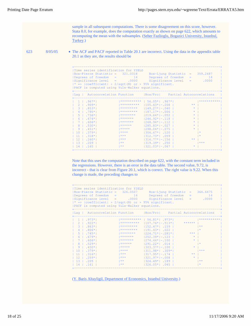
623 8/05/05 The ACF and PACF reported in Table 20.1 are incorrect. Using the data in the appendix table20.1 as they are, the results should be

+----------------------------------------------------------------------------+|Time series identification for YIELD ||Box-Pierce Statistic = 321.0318 Box-Ljung Statistic = 359.2487 ||Degrees of freedom = 14 Degrees of freedom = 14 ||Significance level = .0000 Significance level = .0000 ||* => |coefficient| > 2/sqrt(N) or > 95% significant. ||PACF is computed using Yule-Walker equations. |+----------------------------------------------------------------------------+|Lag | Autocorrelation Function |Box/Prc| Partial Autocorrelations |+----------------------------------------------------------------------------+| 1 | .967*| |*********** | 56.05*| .967*| |***********|| 2 | .909*| |********** |105.63*|-.208 | ** | || 3 | .853*| |********* |149.27*|-.040 | * | || 4 | .795*| |********* |187.17*|-.006 | * | || 5 | .736*| |******** |219.64*|-.052 | * | || 6 | .674*| |******* |246.92*|-.118 | * | || 7 | .606*| |******* |268.94*|-.112 | * | || 8 | .530*| |****** |285.83*|-.027 | * | || 9 | .451*| |***** |298.04*|-.075 | * | || 10 | .379*| |**** |306.67*| .120 | |* || 11 | .318*| |*** |312.73*| .059 | |* || 12 | .260*| |*** |316.77*|-.156 | ** | || 13 | .209 | |** |319.39*| .250 | |*** || 14 | .165 | |** |321.03*|-.067 | * | |+----------------------------------------------------------------------------+

Note that this uses the computation described on page 622, with the constant term included inthe regressions. However, there is an error in the data table. The second value, 9.72, isincorrect - that is clear from Figure 20.1, which is correct. The right value is 9.22. When thischange is made, the preceding changes to

+----------------------------------------------------------------------------+|Time series identification for YIELD ||Box-Pierce Statistic = 326.0507 Box-Ljung Statistic = 364.6475 ||Degrees of freedom = 14 Degrees of freedom = 14 ||Significance level = .0000 Significance level = .0000 ||* => |coefficient| > 2/sqrt(N) or > 95% significant. ||PACF is computed using Yule-Walker equations. |+----------------------------------------------------------------------------+|Lag | Autocorrelation Function |Box/Prc| Partial Autocorrelations |+----------------------------------------------------------------------------+| 1 | .973*| |*********** | 56.81*| .973*| |***********|| 2 | .922*| |********** |107.76*|-.513*| ****** | || 3 | .863*| |********* |152.47*| .159 | |** || 4 | .806*| |********* |191.43*| .022 | |* || 5 | .745*| |******** |224.71*|-.281*| *** | || 6 | .679*| |******* |252.39*|-.123 | * | || 7 | .606*| |******* |274.44*|-.100 | * | || 8 | .529*| |****** |291.22*| .014 | |* || 9 | .450*| |***** |303.37*|-.100 | * | || 10 | .379*| |**** |311.98*| .309*| |*** || 11 | .316*| |*** |317.95*|-.174 | ** | || 12 | .259*| |*** |321.97*|-.008 | * | || 13 | .205 | |** |324.49*| .189 | |** || 14 | .161 | |** |326.05*| .045 | |* |+----------------------------------------------------------------------------+

(Y. Baris Altayligil, Department of Economics, Istanbul University.)


19 of 25 11/17/2006 9:20 AM

625 08/05/05 In the third item in the list above (20-17), cos(π)=0 should be cos(π)=-1 and sin(π)=1 should be sin(π)=0. (Kei Nanamiya Graduate school of Economics, Hitotsubashi University, Japan.)

635 5/8/03 In the first line of the page, ut should be εt. In (20-21), εt should be vt. Then, the line after(20-21) will be correct, where vt is εt corresponding to (20-18) and (20-20) and (1-L)εtcorresponding to (20-19). Gokhan Ozertan, Bogazici University and Dr. Ernesto SepúlvedaVillarreal, The Bank of Mexico.)

643 9/20/05 In the first equation on the page, the subscript on the left hand side variable should be t, not y.The same error occurs on page 644 in equation (20-23) and on page 645 in the last equation onthe page. (Kei Nanamiya, Graduate School of Economics, Hitotsubashi University, Japan .)

639 7/10/03 In the fourth equation, the term β(1-γ) should be β(1-γ)t. The time trend is missing. (Seher Fazlioglu, Bogazici University, Istanbul, Turkey.)

648 5/4/05 In Example 20.7, the value 0.2505 given in the 5th line should be 0.2443. The standard errorgiven, 0.225 should be 0.2221. (Professor Houston Stokes, University of Illinois, Chicago.)

671-672 3/11/03 In the last equation on the page, λi0 should be λ0i and λi

1 should be λ1i. On 672, in (21-24) and in the last line of the page, λi1 should be λ1i. (Paul Glewwe, University of Minnesota.)

667 1/20/05 In the 5th line after equation (21-7), Weibull should be Gumbel. In the immediately followingequation, exp[-exp(x'β)] should be exp[-exp(-x'β)]. In the next equation, 1-exp[exp(-x'β)]should be 1-exp[-exp(x'β)]. (Dr. Tomoo Higuchi, Policy Research Institutes, Ministry of Agriculture, Forestry and Fisheries, Tokyo.)

667 5/20/05 In the 8th line after the third equation, "y = 0" should be "Y = 1". In the next line, "smallerprobabilities to Y = 0" should be "smaller probabilities to Y = 1". (Jenny Nykvist, Department of Economics, Uppsala University, Sweden.)

671 3/20/05 In equation (21-19), the β in the denominator at the left of the equals sign should be boldface.(Hai-Anh H. Dang, University of Minnesota.)

671 3/20/05 In the second line of footnote 6, the xi should be followed by a prime. (Hai-Anh H. Dang, University of Minnesota.)

675 1/31/06 In Table 21.1, the rightmost header Weibull should be Gumbel. In the fifth column, the value0.499 should be 0.450. In the second line of the second paragraph of Example 21.3, "Weibull"should be "Gumbel." (Dr. Tomoo Higuchi, Policy Research Institutes, Ministry of Agriculture, Forestry and Fisheries, Tokyo and Professor Haim-Dov Fried, Stern School of Business, NYU)

675 6/08/05 In equation 21-25, a possibility ambiguity is removed by placing d=1 and d=0 in parentheses.(Marcus Opp, Graduate School of Business, University of Chicago.)

681, 684, 685

3/11/03 (Not an error - just an unexplained change in notation.) In (21-31) on 680, in the second to last equation on page 684, and in the second to last line on page 685, the text uses β'x whereas everywhere else, it uses x'β. The two are equivalent. For consistency, the notation could bechanged. (Paul Glewwe, University of Minnesota.)

681 3/30/03 Eight lines up from the end of the page, in the "428 observations with kids=1 and the 325...,"the 428 should be 524 and the 325 should be 229. The other results given are correct. (Carter Hill, Lousiana State University.)


20 of 25 11/17/2006 9:20 AM

684 3/11/03 In the third line after the first equation on the page, "vary badly" should be "very badly." (Paul Glewwe, University of Minnesota.)

686 4/27/03 In the last equation on the page, the argument of the function should be xi'β. (Not an error, justinconsistent with the rest of the text.) (Eric Isenberg, Department of Economics, Washington University in St. Louis.)

687 4/27/03 In equation (21-39), three occurrences of πi should be xi'β. (Eric Isenberg, Department of Economics, Washington University in St. Louis.)

688 4/27/03 In the first line of footnote 24,the upper case P should be lower case. (Eric Isenberg, Department of Economics, Washington University in St. Louis.)

690 12/15/02 In footnote 27, the reference to Hsiao (1996) should be (1986) twice. (Steve Olley, National Economic Research Associates.)

695 9/06/04 In the last equation on the page, after the second equals sign, the summation over i = 1,...,n is missing - it appears after the first equals sign. (Jun Ma, Department of Economics, University of Washington)

698 and 990

4/21/05 The reference on page 698 to Anderson (1970) should be to Andersen (1970). On page 960,the bibliography entry for Anderson, E., ..., (1970) should be to Andersen, D., ... (Wolfgang Hess, University of Hohenheim, Germany. .)

702 9/24/04 Six lines up from the end of the page, "can used to provide" should be "can be used toprovide". (Erhan Uluceviz from Bogazici University, Istanbul/Turkey.

711 3/20/05 In the first equation on the page, at the end of the line, the subscript on ρ should be i* not t*.(Hai-Anh H. Dang, University of Minnesota.)

713 12/15/02 In the last equation on the page, "y2=2" should be "y2=1". (William Greene, NYU/Stern)

720 04/15/03 In the third equation on the page, after the second equals sign, the two occurrences of αishould not have subscripts. (Simon Jackman, Political Science, Stanford.)

721 11/01/05 In equation (21-46), j=0,1,2,...,J. (Hai-Anh Dang, University of Minnesota)

722 11/01/05 Two lines up from the expression for the asymptotic variance, γ0 should be δ0. (Hai-Anh Dang, University of Minnesota)

723 11/01/05 In equation (21-48) all occurrences of z should be x. (Hai-Anh Dang, University of Minnesota)

727 11/01/05 In the last equation on the page, the choice should be conditioned on x and the two inequalities should be reversed. (Hai-Anh Dang, University of Minnesota)


21 of 25 11/17/2006 9:20 AM

728 3/7/06 In the discussion of constructing the matrix Σ using SRS, it is stated that "R is otherwise restricted only in that -1 < Rjl < +1. The resulting matrix must be positive definite." This is nottrue. M. Bontch-Osmolovski provides the example S=diag(1,2,3) and R=[1 ,-0.5, 0.5/-0.5, 1, 0.8/0.5, 0.8, 1 ). The resulting matrix has a distinctly negative characteristic root. There are noobvious formulaic restrictions that can be given for the general R matrix. The condition givenin the text is necessary, but not sufficient. (Misha Bontch-Osmolovski, Department of Economics, UNC-Chapel Hill..)

764 11/01/05 In the box for Theorem 22.4, in the last line, the x in the denominator of the derivative shouldbe bold instead. (Hai-Anh Dang, University of Minnesota)

730 3/30/03 In the first column of values given in Table 21.11, the -0.19612 should be -0.09612. (Carter Hill, Lousiana State University.)

740 3/11/03 In the first equation on the page, which defines the Poisson density, Prob(Yi=yi|xi) should beProb(yi=j|xi), in the exponent on λ, yi should be j, and yi=0,1,2,.... should be j=0,1,2,....,

742 6/08/05 In the second line after the first equation, "... it can fall..." should be "... it can rise ..."

(similarly to an adjusted R2. (Marcus Opp, Graduate School of Business, University of Chicago.)

747 6/08/05 In the second and third equations on the page, the upper limit in the summations should be Ti.In the third equation on the page, both occurrences of 1/n should be 1/Ti. (Prof. Regina T. Riphahn, Deptartment of Economics, University of Erlangen, Germany .)

750 4/29/03 The last (unnumbered) equation on the page should beE[yi|xi] = (1-Fi) x 0 + Fi x E[yi*|xi,regime 2] = Fi x λi.(Sung Ho Park, Department of Political Science, Texas A&M University)

759-760 11/1/02 (The following analysis was suggested by Gregory Colman of the Graduate Center at the CityUniversity of New York. He submitted it with reference to the fourth edition, but the examplewas repeated in the fifth, so his suggestion is reported here, instead.)In Example 22.2, you state that since E[income|income > 100] =142, we can infer that E[logincome | log income > log(100)] = log(142). Or, generally,

(1) E[ex | ex > ea] = eb <=> E[x | x > a] = b,where a = log(100) and b = log(142). But, by setting a = 0, it is clear that this is not correct, asexplained in the section on the lognormal distribution. The correct expression for a normally

distributed variable with mean mu and variance sigma2 would be

E[ex | ex > ea] = exp[mu + .5sigma2] times PHI(sigma-z)/PHI(-z)

where z = (a - mu)/sigma. Setting this equal to eb and using the other equation, z = PHI-1(p) where p = 0.98 gives an estimate of mu = 2.8949 and sigma = 0.8327. Professor Colmanchecked this by generating 500,000 observations from the normal population with theseparameters and "got all the right results." The implied mean income is $25,576 which nearlymatches the Census number of $25,000 cited in the example.

760 10/16/03 In the discussion after (22-8), the reference to the "truncated variance" actually refers to thescale factor in the truncated variance, (1 - δi), not the variance, which is this scale factor times

σ2. (Hai-Anh Dang, University of Minnesota)

761 10/16/03 In the first and third lines after (22-9), "22-7" should be "22-7." (Hai-Anh Dang, University of Minnesota)


22 of 25 11/17/2006 9:20 AM

766 7/18/03 Just above the second equation on the page, Robert Moffitt's name is misspelled. The second 'f'is missing. (Seher Fazlioglu, Bogazici University, Istanbul, Turkey)

766 6/10/05 In the definitions after the second equation on the page, αi should be divided by σ. αi=xi'β/σ.(Marcus Opp, GSB, University of Chicago.)

771 11/21/05 The elements in the vector di are not defined correctly. They should be as follows (based onthe results on page 41 of Chesher and Irish (1987) referenced in the text):εi = yi - xi'β αi = [(li - xi'β)/σ] where li is the lower censoring limit, usually zero,ai=[(yi - xi'β)/σ]λi = φ(αi )/Φ(αi ), where φ(.) is the standard normal pdf and Φ(.) is the standard normal cdf,e1 = -D0i λi + D1i ai,

e2 = -D0i αiλi + D1i (ai2 - 1),

e3 = -D0i (2+αi2)λi + D1i ai

3,

e4 = -D0i (3 αi + αi3)λi + D1i (ai

4 - 3),and, finally, D0i is one if y is less than the limit value and zero otherwise and D1i = 1 - D0i.The remainder of the discussion is correct. Doing the computations indicated for the Fairdata/model in Table 22.3 produces a chi-squared statistic of 4.31149. The following LIMDEPcode was used to carry out the test. Chen-Chang Lo reports the same result using a user defined procedure in Stata.

Create ; d1=(y=0) ; d2 = 1-d1$Namelist ; x=one,z2,z3,z5,z7,z8 $Create ; e=y-x'b ; alpha=-x'b/s ; a=e/s ; l = n01(alpha)/phi(alpha) $Create;e1=-d1*l+d2*a;e2=-d1*alpha*l+d2*(a*a-1);e3=-d1*(2+alpha^2)*l+d2*a^3;e4=-d1*(3*alpha+alpha^3)*l+d2*(a^4-3)$Create ; dd1=e1 ; dd2=e1*z2 ; dd3=e1*z3 ; dd4=e1*z5 ;dd5 =e1*z7 ; dd6=e1*z8 ; dd7=e2 ; dd8=e3 ; dd9=e4 $Namelist ; d=dd1,dd2,dd3,dd4,dd5,dd6,dd7,dd8,dd9 $Matrix ; list;v=1'd*Ginv(d'd)*d'1$

(Chen-Chang Lo, University of Birmingham, UK.)

776-780 0/7/05 Several corrections to numerical results in Tables 22.3, 22.4, 22.5 and 22.6:In Table 22.3, the Tobit constant term should be 8.17, not 8.18;In Table 22.3, the Probit constant term should be 0.977, not 0.997;In Table 22.4, the Left censored constant term should be 8.17, not 8.18;In Table 22.4, the standard error should be 2.74, not 0.797;In Table 22.5, the seven standard errors for the negative binomial results, beginnning with0.859, should all be changed to, respectively, 0.664, 0.0192, 0.0350, 0.111, 0.0702, 0.111,0.786;In Table 22.5, in the censored negative binomial results, the values 9.39 and 1.36 should be9.40 and 1.35, respectively;In Table 22.6, The marginal effects for the ZIP model should all be changed to -0.0216,0.0702, -0.210, 0.0467, -0.273, respectively moving down the column.(Aurora Alonzo Anton, University of the Basque Country, Bilbao, Spain..)

784 3/12/04 In section 22.4.3, in point 1., in the third line, in the expression for delta-hat, the minus signinside the parentheses should be a plus sign. (Tom Doan, Estima)

786 2/10/06 In Table 22.7, the standard error reported for the estimate of (ρσ) of 0.127 should be 1.2667.All of the values reported for Maximum Likelihood are incorrect. The column of estimatesshould be, in order, (-1.963,0.0279,-0.000109,0.457,0.447,-0.132,3.108). The column ofestimated standard errors should be, in order,


23 of 25 11/17/2006 9:20 AM

(1.684,0.0756,0.0023,0.0964,0.427,0.224,0.0837). (Tom Doan, Estima (Reported 3/12/04)) Inthe final column, the standard error of 0.449 reported for the estimator of β5 should be 0.318.(Dr, Tomoo HIGUCHI, Policy Research Institutes, Ministry of Agriculture, Forestry and Fisheries Tokyo/Japan)

789 3/11/03 Four lines up from the end of the page, the references (1999,2000) should be (1997,2000).(Paul Glewwe, University of Minnesota.)

795 9/27/05 In the second equation, the term after the first summation sign should be ln?(t|?) . (Yuanzhu Lu, Department of Economics, National University of Singapore)

799 9/27/05 In the third equation on the page, the minus sign inside the parantheses should not be there.(Yuanzhu Lu, Department of Economics, National University of Singapore)

822 7/25/03 At the end of line 2 of Section A.4.4, "Let z equal..." should be "Let a..." (Alan Mehlenbacher, Expert Decision Software.)

803 7/25/03 There is some test missing at the end of the fourth bullet entry, "For example," should be "Forexample, I3 denotes a 3 by 3 identity matrix." (Alan Mehlenbacher, Expert Decision Software.)

840 2/17/05 In the first equation after (A-133), in Aji, the ji should be ij. In the next equation, C is already

signed by the definition, so the (-1)i+j should be deleted. Finally, in the next equation, Cjishould be Aij. (Giuseppe Vittucci, Italy)

844 8/10/03 In the second to last equation on the page, the matrix of derivatives should be preceded by"abs(det(" and succeeded by "))." I.e., we need to take the absolute value of the determinant.(Alan Mehlenbacher, Expert Decision Software.)

851 9/30/03 In the text above the last bullet item on the page, "upper (right) tail areas" should read "lower(left) tail areas." (Ila Alam, Department of Economics, Tulane University.)

865 6/26/03 In Theorem B.2, in (B-67), there is close square bracket missing in the middle term. (Erhan Uluceviz from Bogazici University, Istanbul/Turkey.)

866 8/10/03 In the paragraph which follows the box containing (B-68), in the second sentence, "which alsoappears" should be "which also appear". (Alan Mehlenbacher, Expert Decision Software.)

870 4/6/04 In the last two equations, in E[g(x)] and Var[g(x)], the "g" should be bold, not italic. (Mr. Spanos Andreas, University of Exeter.)

889 11/5/04 In equation (C-12), in the denominator of the derivative in square brackets at the left of theequals sign, the superscript 2 should appear after theta, not before it. (Ramiro A. MálagaOrtega, Departamento de Economía, Pontificia Universidad Católica del Perú.)

895 4/6/04 In the fourth line of Example C.11, in the expression H1: µ=µ0, the equals sign should ne "notequals." (Mr. Spanos Andreas, University of Exeter.)

901 4/6/04 In the last line of Theorem D.7, the xn should have an overbar. (Mr. Spanos Andreas, University of Exeter.)


24 of 25 11/17/2006 9:20 AM

901 6/21/04 In the fourth line of the paragraph after Theorem D.3, the convergence almost surely to xshould be convergence a.s. to c. (Ilton G. Soares, Federal University of Ceara - CAEN, Fortaleza - Ceara - Brazil.)

901 and 905

10/3/02 Definition D.3 for Almost Sure Convergence is not correct. Treatments vary a bit by author,but a consensus would state that For any ε, Prob(limn->inf xn = c) = 1.In order to write this in a form that facilitates comparison to the definition of convergence inprobability that appears on page 897, we might uselimn->inf xn = c => limn->inf |xn - c| < ε for all ε > 0.Then, almost sure convergence can be seen to be arise from the definition of convergence inprobability by moving the limit operation inside the operation of the probability function (andallowing ε to be zero). In the discussion after D.3 on page 901, it is then necessary to delete thetwo sentences "Note that the index ..." and "The event described in the definition ..." On page905, Definition D.7 is the same as D.3, but c is now changed to random variable, x. (The need to revise these definitions was pointed out by Castedo Ellermann and Nicholas Levi,Department of Mathematics, NYU..)

902 4/6/04 In the second line of the corollary to Theorem D.8, the xn should have an overbar. (Mr. Spanos Andreas, University of Exeter.)

902 11/15/04 In footnote 2, in the third line, E[z|z<0] should be E[-z|z<0]. In the same line, 0.7989 should be0.7979. (Hai-Anh H. Dang, University of Minnesota.)

903 4/6/04 In Theorem D.11, in the first and third lines, the references to Theorem D.9 should be toTheorem D.10. (Mr. Spanos Andreas, University of Exeter.)

906 4/6/04 In Definition D.10, "distribution of x" should be "distribution of xn." (Mr. Spanos Andreas, University of Exeter.)

906 6/21/04 In the second line on the page, directly above Definition D.9, the Fn(x) should be Fn(xn) . Inthe first line of Definition D.10, F(xn) should be Fn(xn). (Ilton G. Soares, Federal University of Ceara - CAEN, Fortaleza - Ceara - Brazil.)

908 4/6/04 In the fourth line of Example D.5, the subscript on z should be "j, not n. (Mr. Spanos Andreas, University of Exeter.)

909 4/6/04 In the penultimate line of the first paragraph after Theorem D.18,the reference to Example D.5should be to D.6. (Mr. Spanos Andreas, University of Exeter.)

909 6/21/04 In the first equation in Theorem D.19, in the second equality, the ellipsis (...) should be

followed by σn2. (Ilton G. Soares, Federal University of Ceara - CAEN, Fortaleza - Ceara -

Brazil.)

910 4/6/04 In the fourth line up from the end of the page, the reference to Theorem D.12 should be toD.19. (Mr. Spanos Andreas, University of Exeter.)

912 4/6/04 In the fifth line of the second paragraph after Theorem D.20, the reference to Example D.5should be to D.6. (Mr. Spanos Andreas, University of Exeter.)

919 4/6/04 In the second line of the second paragraph after Definition D.15, the reference to Section C.3should be to D.3. (Mr. Spanos Andreas, University of Exeter.)


25 of 25 11/17/2006 9:20 AM

922 3/12/04 In footnote 4 on this page, B.7.11 should be A.6.11. (Sylvain Friederich Department ofEconomics, University of Bristol.)

923 10/16/03 In the first line of Example E.1, "D.7" should be "D.8." (Hai-Anh Dang, University of Minnesota)

947 2/17/05 The Mroz data set contains a variable not given in the list, MTR = the wife's marginal tax rate.(Giuseppe Vittucci, Italy)

949 12/15/02 The data table for the airline data has C and Q reversed. The results in the text have the datacorrectly arranged. The data on the Prentice Hall website are mislabeled. The data on thiswebsite are correct. (Steve Olley, National Economic Research Associates.)

952 9/19/05 In the documentation for data table F21.4, in the definition of Depndt, the variable isdependents, not one plus the number of dependents. Inc_Per is income divided by one plus thenumber of dependents, not income divided by the number of dependents. Within the data set,itself, there are seven maverick observations, 79, 324, 435, 462, 656, 659, 1195, in which age,in years, is obviously miscoded. The values .5, .1667, .5833, .75, .5833, .5, .75 are obviouslyerroneous. The correct values are lost to antiquity, though it appears that observation 79, basedon its appearance in Table F9.1, should be 36. The others are unknown. (Christian Kleiber, University of Dortmund, Germany.)

953 3/5/05 Table FD.1 is missing E=Education.

977 3/11/03 The 1986 reference for Hensher should be changed to Hensher, D. "Sequential and Full Information Maximum Likelihood Estimation of a Nested-Logit Model." The Review of Economics and Statistics, LXVII, 4, 1986, pp. 657-667.

978 02/65/06 In the reference to Jennrich, the journal should be The Annals of Mathematical Statistics.Tamer Kulaksizogly.

984 4/19/06 The first reference for McFadden should be 1974a, not 1973. The second should be 1974b, not1974. (Kit Baum, Department of Economics, Boston College.)

990 11/15/04 In the bibliography, two references to V. Srivistava should be to V. Srivastava. Arne Henningsen, Department of Agricultural Economics, University of Kiel.

993 5/2/03 The last reference on the page, "Wynand and B. van Praag..." should bevan de Ven, W.P.M.M. and van Praag, B.M.S., "The Demand for Deductibles in PrivateHealth Insurance: A Probit Model With Sample Selection," Journal of Econometrics, 17, 1981, pp. 229-52. (Olle Westerlund, Department of Economics, Umea University.)

994 4/20/03 The ReStat, 66, 1984 reference for Yatchew and Griliches should be 67, 1985. (Bill Becker, Economics, Indiana University.)

econometric analysis, 5th edition - agricultural & applied economics

Documents