transportation costs in econometric models of state agricultural

Transportation Costs in Econometric

Models of State Agricultural Sectors:

The Case of Beef in Hawaii

Roland K. Roberts

Econometric models designed to show how national policies affect state agricultural sectorsoften use national prices as proxies for state prices. Consequently, they ignore the influence offreight rates on state production. An application to the Hawaii beef industry demonstrates thatboth freight rates and national beef prices have important impacts on Hawaii beef prices andproduction. By using state prices rather than national prices, error from changes in freight ratesmight be reduced, and the model's capacity for policy analysis might be broadened.

Interest has grown in developing stateeconometric models for policy analysis(Knapp et al.). For a state agriculturalmodel to be useful for a wide range ofpolicy analyses, it should be able to indi-cate state-level impacts of changes in bothstate and national policies. Baum et al.employed such a model to analyze the im-pacts of U.S. beef import policy on theVirginia beef and pork sectors. However,they used national prices in their beef andhog production equations instead of Vir-ginia prices. Such an approach can bias astate model and subsequent impact anal-yses. If prices are not totally transmitted

Roland K. Roberts is an Associate Professor, Depart-ment of Agricultural Economics and Rural Sociolo-gy, University of Tennessee. This research was con-ducted while the author was at the University ofHawaii.

The author is grateful to Peter Garrod and JohnRoecklein for their contributions toward the devel-opment of this paper. The suggestions of the anon-ymous reviewers are also appreciated. This researchcontributes to Western Regional Project W-145. Ha-waii Institute of Tropical Agriculture and HumanResources Journal Series Number 2888.

within the current period, or if there is atransportation cost differential betweennational and state prices, the use of stateprices estimated through price transmis-sion equations might reduce that bias.Furthermore, the impact information ob-tainable from a state model would in-crease as the array of policy variables isaugmented by transportation costs.

An econometric model of the Hawaiibeef industry is used as a case study todemonstrate the potential improvement inimpact analysis by state econometricmodels that use state rather than nationalbeef and feed prices. The specific objec-tives of this paper are 1) to demonstratethe importance of transportation costs asdeterminants of Hawaii beef and feedprices; 2) to illustrate that introducingtransportation costs may eliminate a spec-ification bias and render greater reliabili-ty to subsequent impact analysis; and 3)to demonstrate the augmented policyanalysis capabilities of a state agriculturalcommodity model that includes transpor-tation costs and national prices in its stateprice transmission equations.

Hawaii provides a unique setting forexamining the importance and usefulness

Western Journal of Agricultural Economics, 10(1): 93-109© 1985 by the Western Agricultural Economics Association

Western Journal of Agricultural Economics

of transportation costs in state commoditymodels. It is located about 2,500 milesfrom the rest of the United States. Thisisolation leads to a richness of data in thattransportation costs are typically higherthan for other states and more easily iden-tified. Hawaii can be thought of as theextreme case. If transportation costs arenot important in determining Hawaii beefand feed prices, they are unlikely to beimportant in determining those prices inother states.

Whether transportation costs are im-portant price determinants is an empiricalquestion that depends on each state's orregion's location relative to major mar-kets. For example, the Omaha utility cowprice was used in the Baum et al. modelto determine Virginia beef cattle slaugh-ter. Whether there was a significant trans-portation cost differential between Oma-ha and Virginia utility cow prices was notaddressed.

In this analysis, Hawaii beef and feedprices are estimated as a function of LosAngeles beef and corn prices and Los An-geles-to-Honolulu freight rates. Althoughthe data and results are specific to Ha-waii's beef production sector, this paper'sapproach can be adapted to any state orregion in which prices are determined ex-ogenously and freight charges are rela-tively important. A similar method maybe appropriate for a number of develop-ing nations that import a significant pro-portion of a commodity.

The importance of transportation costsas determinants of Hawaii beef and feedprices is stressed through regression anal-ysis, and the Hawaii beef model is brieflyoutlined. Three versions of the model aresimulated to emphasize differences in es-timated impacts when transportation costsare not considered. The model's improvedpolicy analysis capabilities are also dem-onstrated under various assumptions aboutchanges in transportation cost variables.Finally, implications and general conclu-sions are drawn.

Transportation Costs asDeterminants of Hawaii Prices

The Hawaii Agricultural ReportingService estimated that 1980 beef importsfrom the Mainland United States and for-eign sources (Australia and New Zealand)accounted for 53 and 16 percent, respec-tively, of total Hawaii beef market supply.However, imports to Hawaii from theMainland were only about 0.2 percent ofMainland production and 1.3 percent ofAustralian and New Zealand exports to theentire United States (Schermerhorn et al.).Because of Hawaii's insignificance in na-tional and international markets, Hawaiibeef prices are assumed to be determinedexogenously. The demand for beef in Ha-waii has little impact on local beef prices.The difference between the Hawaii de-mand for beef and local production, at theexogenously determined price, can easilybe augmented by imports from the Main-land and foreign sources. Because of thedominance of imports in the Hawaii mar-ket and the influence of the United Statesas a pricemaker in international beef mar-kets (Simpson, p. 1), it follows that whole-sale prices of Hawaii-produced beef shouldbe closely related to Mainland prices andtransportation costs. Similarly, the price offeed in Hawaii is assumed to be deter-mined by Mainland price and transpor-tation costs. On the other hand, exoge-nously determined prices influenceproduction decisions in Hawaii, allowingtransportation costs to affect Hawaii beefproduction.

Four equations were specified to reflectbeef and feed price transmission from theMainland United States to Hawaii. Ex-planatory variables included current andlagged Los Angeles prices and oceanfreight rates from Los Angeles to Hono-lulu. Quarterly dummy variables were alsoincluded because seasonal variation instate, national and international beef mar-kets were expected to influence pricetransmission. Each equation was first es-

94

July 1985

Transportation Costs in State Models

timated by ordinary least squares. Theresiduals were used to calculate the Dur-bin-Watson statistic (DW) and a similarstatistic (D4) designed to test for fourthorder autocorrelation (Wallis). Where sig-nificant first order autocorrelation was in-dicated, a Cochrane-Orcutt autoregres-sion procedure was used to obtain moreefficient parameter estimates. Lag struc-tures were not specified a priori. There-fore, in equations where lags in pricetransmission were hypothesized, the num-ber of lags was determined by includingsuccessively longer lags until the coeffi-cient of the final lag became negative ornegligible relative to its standard error.

The final price transmission equations(Equations 1A-4A) are presented in Table1. The R2 are all greater than 0.96, sug-gesting that the explanatory variables pro-vide a good fit (Kmenta, p. 234). In nocase does the D4 statistic indicate signifi-cant fourth order autocorrelation at the 5percent level and seasonal effects are onlysignificant in the grass-fed steer and heiferprice transmission equation (Equation3A). 1

Ocean freight rates are used in Equa-tions 1A-4A because time-series on totaltransportation costs for beef and feed fromLos Angeles to Honolulu are not readilyavailable. Although ocean freight costsrepresent a significant portion of totaltransportation costs, other logistics costssuch as wharfage fees, land transportationcosts for hauling to and from the docks,and storage can account for perhaps asmuch as one-half of the total cost (Gar-rod). Ocean freight rates can be viewedas proxies for total transportation costs be-cause all transportation costs, whether for

1Seasonal dummy variables were retained in Equa-tions 1A, 2A and 4A for comparison. Reestimationwithout quarterly dummy variables did not appre-ciably affect the coefficients of the remaining vari-ables and the R2 variables only increased slightly.For example, the R2 of Equation 2A increased from0.9847 to 0.9850 when dummy variables weredropped.

land or sea transportation, are highly cor-related with energy and labor costs. Thefreight rate variables are all highly signif-icant, with coefficients ranging from 2.27in the Honolulu choice beef price equa-tion (Equation 1A) to 2.57 in determiningthe price of grass-fed beef (Equation 3A).These coefficients appear large at firstglance, but they are acceptable when oneaccounts for nonocean transportation costs.If the transportation cost variables inEquations 1A-4A were total transporta-tion costs rather than ocean freight rates,the expected size of the coefficients wouldbe about 1.0. Two conditions increase theexpected size of the coefficients. First, ifocean freight costs were one-half as muchas total transportation costs and if otherlogistics costs were highly correlated withocean freight rates, then an increase inocean freight rates by $1.00 per hundred-weight would be accompanied by an in-crease in total transportation costs by$2.00. Hence, the price of beef or feed inHawaii would increase by about $2.00 perhundredweight. Second, the ocean freightrates used in this analysis assume that con-tainers are full, which is not always true.Partially full containers are charged ahigher rate per hundredweight. There-fore, the actual rates are probably higherthan the rates used, further increasing theexpected size of the coefficients.

Given that certain relevant transporta-tion cost variables are omitted, it shouldbe clear that Equations 1A-4A are notpresented as the true price transmissionmodels. The coefficient on the Los Ange-les steer price (LAGFBPRQ) in Equation1A and the sums of the Los Angeles pricecoefficients in Equations 2A-4A are sta-tistically different from unity. Divergencefrom unity might result from a numberof things such as differences in productsand levels of marketing, imperfect pricetransmission or specification error causedby the omission of relevant variables.

Because of local pricing mechanisms,Equation 1A most closely fits the Main-

95

Roberts


co co co CD ) LO ICM - CIJ CI Cf) T

C=; ci6 6 6 Ccc -1 CC-J- CO) CO

I I- I I -

00 CM 1- CV4 06 o oo oC

r- s

0 . L (.COLO't CM o o- T-

CM 0C 0 o0 0I-, 66i 6

cE t -CD r cD00 t O C0 OC

COi CM Co o o (D

CO C) C O C)0 O(D O CO O O CD

CO 0 CM 00000

CE o I- oo66ooC; o Co

-. I. .,

! 0) Oi N -) 040 YO)

cdC o cc c; C ; Co

C 00

C--I C

L) NC 0 CO

_ 1 _c cco 0 co 00

LO a) (D NT- CDC\i o 0 o-

-t '. r. cor- 0) - 0

0-

a) LeV) M 14t )14t co CM Q) r O C

COO)i' -4I.-CO-

0O cO CO CmO O O C)

c c 6 d6c C c c _1-1 I.- 1- 1-

CM C) r- OOr- -O

0 CO C0 CC- O 0) 0h : C5

0CEa. 0a

W m CE0 LL a.

C3 0 04 .1

C C0 LO O

ccI I .

-I- O0C O O

CM O 0 o o oCM CY) 0 LO 0

CdC; c; d C1- -1 I-

T-

a

c001a

CMI

ara.

14

C0I

a

00

aor

00

0

Ian-

O1^

azcr0

15

^ CMINl_- _I

a az z aCe Cc mo O <0 04 ^ c

az

CEHo ao o

July 1985

aLL0

'L c0-t 0

o" °

!- LOCO CM00

Qa)nEzr0Cu

c0w:3V

aCcoa)nCu.u

C

ca)QCC)a>00

mCO

C)

CaCMJ

cm

m

CLaCELLzI

a

I

a

CcL

C)

o(UM0

u,

c

LU

0

0,

E

.i

(U0

0

_.

IL

96

C Cu

-a CX >i^

I

i

<:

<

I


0) Rd,o coo o

0 COO O0 0

0-

COI

CDr- CO C'4

CD CD 0

N.CDT- (DT 0M 0~

D -OD 00)0)00 ' Q) CY)

c; ; : -r ;I.-

0.O Lc TC0066I ~ t1- I-

00CN 0) 00CM 0C O07- T.: c

LO 0) C- 0000 0 0 - 0;o o c; ci ci - co

O c (D CO C o 00) 0) t - O C0)oo C- c\i o

0 00 CO a

0CC co -_COY0)

S ' DC^ CM

00 Q- Q C0

In ' o In o'

!>> z0

ocu

. .a

0

z co

.o

U)

*0 '0

c o~

cCO CeM

E o

U.

C Lo

4. X)0 C

2N '.co 2

U> wE U

o coa

2) E

co 0)

Co Lc

(D a)

) 0) : )<a an a)

o C C

a) j. 0 F a

(u a) >- U)C.o

( E m00E

(o c 2)U,

I > a

*5 )c CD

0a

U) c'4-U)U

·rEo0 *a0.0t))Z

U) CO

land price plus transportation cost model.Once a week the major Hawaii slaughter-houses call slaughterhouses in Los Angelesfor price quotations. Hawaii grain-fedsteer and heifer prices are based on thosequotations plus a markup for transpor-tation costs. The coefficient for the LosAngeles wholesale choice steer price(LAGFBPRQ) is close to unity (0.98) asexpected.2 The coefficient for TRANBQand the constant term suggest that thetransportation cost differential betweenLos Angeles and Honolulu is about 2.27times the ocean freight rate minus $7.18per hundredweight.

Transmission of cow prices from theMainland to Hawaii is more complicatedthan for choice beef. Pricing methods arenot as well defined and, because Hawaiiimports large quantities of cow beef fromAustralia and New Zealand, price trans-mission from the Mainland is indirect viathe Australian and New Zealand markets.Lagged Los Angeles cow prices are in-cluded in Equation 2A to capture pricetransmission delays caused by the greatdistances involved and the time requiredfor changes in the U.S. cow price to workthrough the Australian and New Zealandmarkets to Hawaii. The sum of the coef-ficients on the current and lagged Los An-geles cow prices is 0.94, which is againreasonably close to unity given differencesin products and the indirect transmissionof prices through the Australian and NewZealand markets.

Several factors complicate transmissionof grass-fed steer and heifer beef prices to

2 The true parameter estimated by this regressioncoefficient would be equal to 1.00 only if the LosAngeles and Honolulu prices were for identicalproduct and prices were perfectly transmitted. Inthis case, the Los Angeles price is for steers, whilethe Honolulu price is for steers and heifers. There-fore, the true parameter should be close to unity,but not necessarily equal to unity. The estimatedcoefficient is statistically different from 1.00. How-ever, whether it is close to unity in the same sensethat the true parameter is close to unity is a matterof judgment.

97

m·t

VI

mCO

cO

CDCMJ

aLL0

acr

mzI

3rLm

I

zC0U)

w

(0Ca

c

U0

0a)0.a)I

-dU)

0C)

I-

m

4

o )

Q ciX >w

Roberts

a

rIL

cT -

<

III


Hawaii. First, there are no wholesale grass-fed steer and heifer beef prices in Hawaiior on the Mainland. Second, a dressedweight price received by farmers is re-corded in Hawaii but not on the Main-land. Third, as with cow beef, the Hawaiiprice is determined by the Mainland mar-ket via the Australia and New Zealandmarkets. Because Hawaii-produced grass-fed beef competes with both cow andgrass-fed steer and heifer beef importedfrom Australia and New Zealand, it is hy-pothesized that Mainland steer and cowprices are both highly influential in deter-mining the Hawaii grass-fed steer andheifer beef prices. Equation 3A uses cur-rent and lagged Los Angeles utility cowprices, and current and lagged differencesbetween the Los Angeles choice steer priceand the utility cow price, to represent theinfluence of the Mainland beef market onthe Hawaii grass-fed steer and heifer price.The current and lagged price coefficientsof Equation 3A suggest that, if both LosAngeles prices increased by $1.00, the Ha-waii grass-fed beef price would increaseby $0.64. An increase by $1.00 in the LosAngeles utility cow price or the Los An-geles choice steer price, holding the otherprice constant, would result in increasesin the Hawaii grass-fed beef price of $0.19and $0.50, respectively. These coefficientsseem reasonable given differences in com-modities and levels of marketing.

Mainland prices directly determine theHawaii cattle feed price paid by farmers.Most of the feed used is manufactured inHawaii from feed stuffs imported fromthe Mainland. Relatively little manufac-tured feed is received from the Mainlandfor use by cattle. Pricing methods arepoorly defined. Therefore, current andlagged Los Angeles wholesale corn pricesare used in Equation 4A to capture delaysin price transmission from the Mainlandto Hawaii and from one level in the mar-keting chain to another. The sum of thecurrent and lagged price coefficients is

0.57. This is acceptable given differencesin the levels of processing and marketing.

Equations 1B-4B of Table 1 are iden-tical to Equations 1A-4A except thattransportation cost variables are excluded.These equations suggest that a positive biasmight be present in the price coefficientsresulting from omission of relevant vari-ables. The estimated coefficients of thetransportation cost variables are positiveand highly significant in Equations 1A-4A. Therefore, if prices and ocean freightrates are positively correlated, this omis-sion would likely produce a positive biasin the price coefficients of Equations 1B-4B (Kmenta, pp. 392-95). Price variablesand freight rates are highly correlated. Thesimple correlation coefficients between thebeef freight rate and current and laggedLos Angeles beef prices are all greater than0.80. Similarly, all correlation coefficientsbetween the feed freight rate and currentand lagged Los Angeles corn prices aregreater than 0.65. The consequences ofomitting freight rates are evident. Almostwithout exception the estimated pricecoefficients are larger in Equations 1B-4Bthan in Equations 1A-4A. This is not tosay that Equations 1A-4A are withoutspecification bias. It is clear, however, thatone source of specification error is elimi-nated by including ocean freight rates.These findings suggest that if freight rateswere omitted from a model of Hawaii beefproduction, subsequent impact analyseswould be adversely affected. Differencesin simulated impacts are addressed afterthe Hawaii beef model is briefly pre-sented.

The Hawaii Beef Model

The model used for this analysis hasbeen described in detail (Roberts et al.).The version used in this paper consists of23 equations, 13 of which are behavioralrelationships estimated from quarterly andannual data for 1970 through 1980. The

98

July 1985


model is divided into four sections. Thefirst section deals with Mainland-to-Ha-waii price transmission. For this analysis,Equations 1A-4A of Table 1 replace thefirst seven equations of Roberts et al. Ex-ogenously determined Hawaii beef andfeed prices and an energy price index areused in Section 2 to determine January 1inventories of beef cows, heifers, heifersheld for replacement, heifers not held forreplacement, and steers. The annual calfcrop is also estimated in Section 2. Section3 uses the prices from Section 1 and thecattle inventories generated in Section 2to estimate quarterly production of grain-fed beef, grass-fed steer and heifer beefand cow beef. For completeness, bull beefproduction is also estimated as a functionof cow beef production. Finally, Section4 links the other sections through periodtransition identities that convert quarterlyprices into annual averages for use in Sec-tion 2. January 1 cattle inventories also aremodified for use in the quarterly produc-tion equations of Section 3.

Exogenously determined prices greatlysimplify estimation procedures. The ma-trix of endogenous variable coefficients istriangular, and a recursive system is as-sumed (Johnston). Consequently, ordinaryleast squares and Cochrane-Orcutt auto-regression procedures (White) were usedto estimate the structural equations of themodel. For equations including laggeddependent variables, partial adjustmentwas assumed (Nerlove), and a Grid Searchautoregression procedure was used to ver-ify that the Cochrane-Orcutt procedureconverged to a global maximum of thelikelihood function (Betancourt and Ke-lejian).

Modifications of the Model forImpact Analysis

Simulations of the model over the 1972through 1980 period are used to empha-size differences in simulated impacts and

other problems resulting from the exclu-sion of transportation costs. Three versionsof the model are used. Model I uses Equa-tions 1A-4A to transmit prices from theMainland to Hawaii, while Model II usesEquations 1B-4B for price transmission.All other equations are identical in ModelsI and II. In Model III, all inventory andproduction equations are reestimated, ac-cording to the specification of Models Iand II, using Los Angeles beef and cornprices as regressors rather than Hawaiiprices. Therefore, Model III includes noprice transmission equations. The reesti-mated equations are presented in Table 2for comparison with those of Roberts etal. Symbols are defined in Table 3. UsingLos Angeles prices introduces an addition-al misspecification into Model III. Becausethere are no prices for Los Angeles grass-fed steer and heifer beef, the Los Angelesutility cow price is substituted as a proxyin the grain- and grass-fed beef produc-tion equations. Additional differences inimpacts would result to the extent that apolicy change or other exogenous shockaffected the Los Angeles utility cow pricedifferently from the Hawaii grass-fed steerand heifer price.

Historical Simulations ofModels I-III

Before simulated impacts are mea-sured, the relative abilities of the modelsin tracking historical events are assessedby comparing Theil U2 coefficients (Leu-thold). 3 The U2 coefficients are calculatedfor each model by performing a dynamicsimulation over the 1972 through 1980period. Observations for 1970-71 are ex-cluded to accommodate lags. Each simu-

3 The U2 coefficient is defined in this analysis as

V[(Pt- Atl) - (A, - At-)U2 =

/V(A, - A,_) 2

with Pt being the predicted outcome and At beingthe actual outcome for period t.

99

Roberts


Table 2. Estimated Equations and Identities of the Hawaii Beef Econometric Model UsingNational Rather Than Hawaii Prices (Model III).a

Equationnumberb Equation

I. Quarterly Price Transmission Equationsc

II. Annual Cattle Inventory and Calf Crop Equations

5(9) BCI = 16.716 + .045LAGFBPR(-1)/LACFPI(-1)(35.429) (.060)- .0090LP(- )/LACFPI(-1) + .769BCI(-1),

(.010) (.342)R2 = .7607, DHd, OLS.

6(10) HI = -22.895 + .481CC(-1) .046LAGFBPR(- 1)/LACFPI(-1)(8.549) (.095) (.016)

+ .0120ILP(-1)/LACFPI(-1) + .759HI(-1),(.002) (.120)

R2 = .7942, AUT, = -.541.(.261)

7(11) OHI = -5.016 + .801(HI - HHDCR) - .011LAGFBPR(-1)/LACFPI(-1)(2.785) (.070) (.008)

- .0090ILP(-1)/LACFPI(-1),(.001)

R2 = .9651, AUT, = -.432.(.272)

8(12) HHBCR = HI - OHI - HHDCR.

9(13) SI = -15.249 + .459CC(-1) - .045LAGFBPR(-1)/LACFPI(-1)(10.038) (.134) (.021)

- .0020ILP(-1)/LACFPI(-1) + .553S1(-1),(.004) (.189)

R2= .8660, AUT, = -. 392.

(.307)

10(14) CC = -34.757 + .899(BCI + DCI) + .784(HHBCR + HHDCR),(24.931) (.183) (.375)

R2= .7275, AUT, = -. 426.

(.273)

III. Quarterly Beef Production Equations

11(15) GFBPQ = -5,762.6 - 78.756TSOHIQ*D1Q- 53.088TSOHIQ*D2Q(1,601.2) (27.609) (20.988)

+ 24.960TSOHIQ*D3Q + 67.072TSOHIQ(15.976) (26.428)

+ 62.258TSOHIQ(-4)*D1Q + 450.01RSOHIQ*D1Q(24.560) (560.10)

+ 1,346.2RSOHIQ*D2Q - 958.72RSOHIQ*D3Q + 3,636.8RSOHIQ(726.57) (542.60) (834.32)

+ 47.503LAGFBPRQ(-1)/LACFPIQ(-1)- 26.142LACPRQ(-1)/LACFPIQ(-1)(11.835) (10.670)

- 5.7500ILPQ(-1)/LACFPIQ(-1)(1.529)1 0.520[LAGFBRQ(-1 )/LACFPIQ(- 1) - LAGFBPRQ(-2)/LACFPIQ(-2)](6.049)

100

July 1985


Table 2. Continued.

Equationnumber b Equation

+ 4.639[OILPQ(-1)/LACFPIQ(-1) - OILPQ(-2)/LACFPIQ(-2)](1.675)

+ 892.89DM1Q + 756.36DM2Q - 432.30DM3Q - 476.75WQ + 38.529TQ,(215.38) (190.64) (303.21) (130.69) (14.823)

R2 = .9499, AUT, p = .328.(.151)

12(16) NFBPQ = 405.96 - 1.114TSOHIQ*D1Q + 4.197TSOHIQ*D2Q(343.01) (1.034) (.713)+ 2.456TSOHIQ*D3Q + 22.595TSOHIQ - 229.03RSOHIQ

(.999) (5.095) (156.92)- .141GFBPQ(-3) - 11.392LAGFBPRQ(-3)/LACFPIQ(-3)

(.031) (2.580)+ 9.837LACPRQ(-3)/LACFPIQ(-3) + .76501LPQ(-3)/LACFPIQ(-3)

(2.611) (.314)- 44.668WQ(-3) + 247.47DM3Q + .629NFBPQ(-1),

(31.089) (59.849) (.093)R2 = .9164, AUT, = -. 388.

(.157)13(17) TSHBPQ = GFBPQ + NFBPQ.

14(18) CBPQ= 3,396.5 - 1.147CIQ*D1Q + 1.014CIQ*D2Q + .457CIQ*D3Q(981.95) (.484) (.484) (.411)

- 17.596CIQ + 3.691 [LACPRQ/LACFPIQ - LACPRQ(-1 )/LACFPIQ(-1)](9.282) (4.271)

- 1.825[LAGFBPRQ/LACFPIQ - LAGFBPRQ(-1 )/LACFPIQ(-1)](3.532)

- 8.743TQ + 75.779WQ,(3.216) (47.959)

R2= .6013, AUT, p = .380.(.141)

15(19) BBPQ = 36.171 + .046CBPQ + 44.798D1Q + 20.981D2Q(64.666) (.038) (15.8148) (15.920)+ 31.267D3Q + .459BBPQ(-1),

(15.296) (.142)R2 = .3190, DH =-.851, OLS.

16(20) TBPQ = TSHBPQ + CBPQ + BBPQ.

IV. Period Transition Identities4

17(21) LACFPI(L)e = .25 LACFPIQ(t).t=l

4

18(22) LAGFBPR(L) = .25 LAGFBPRQ(t).t=i

4

19(23) OILP(L) = .25 S OILPQ(t).t=1

20(24) CIQ(t = 1-4)= BCI(L) + DCI(L).

101

Roberts


Table 2. Continued.

Equationnumberb Equation

21(25) TSOHIQ(t = 1-4)= SI(L) + OHI(L).

22(26) RSOHIQ(t = 1-4) = S(L)/OHI(L).

a In the autoregressive equations (AUT), R2 is viewed only as a measure of goodness-of-fit (Kmenta, p. 234).Numbers in parentheses below coefficients are estimated standard errors (asymptotic standard errors for AUTequations). Numbers in parentheses following variable names indicate lags. Variables are defined in Table 3.

b Numbers in parentheses following equation numbers indicate the corresponding equation in Roberts et al.c Price transmission equations are not used in this version of the model.d Calculation of Durbin's h statistic was not possible.e L refers to the current year and t refers to the quarter of that year.

lation is performed by allowing the modelto iterate, with exogenous variables set athistorical levels and lagged endogenousvariables set at predicted values. Thesesimulations are used as bases for calculat-ing simulated impacts in the next section.

The U2 coefficients calculated from themodels are presented in Table 4. Whencomparing models, lower U2 coefficientsindicate greater accuracy. The U2 coeffi-cients are lower for Model I than forModels II and III, with the exception ofbull beef production (BBPQ), for whichthe U2 coefficient is lowest for Model II.In no case is the U2 coefficient smaller forModel III than for Models I or II. Thesecomparisons demonstrate (1) that the ex-clusion of transportation costs from theprice transmission equations substantiallydecreases the accuracy of the model and(2) that elimination of price transmissionequations further reduces the model'sgoodness-of-fit to historical data.4

4 The inventory and production equations of ModelsI and II were theoretically specified and adjustedaccording to goodness-of-fit criteria (eg., iR

2 , stan-dard error and signs of the coefficients) and dataavailability. Had the same criteria been used to ad-just the inventory and production equations ofModel III, it is possible that a better fitting model,with a different structure, would have been devel-oped. However, given the exclusion of freight rates,the lack of a Los Angeles grain-fed steer and heiferprice, and other data limitations, it is unlikely thatsuch a model would have U2 coefficients lower thanthose of Model I.

Differences in Impacts

Several additional simulations are con-ducted to emphasize differences in simu-lated impacts among the models. Subse-quent simulations for a particular modelare compared to their respective bases.Impacts are defined as deviations from thebase. Three additional simulations areperformed with each model. Each addi-tional simulation increases one of the threeLos Angeles prices by 10 percent aboveannual historical levels, while other vari-ables are kept at base values.

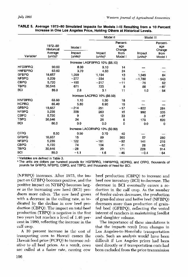
Table 5 contains the simulated impactsof key variables, averaged over the simu-lation period (1972-80) to conserve space.Before impacts are compared among themodels, it is helpful to describe brieflythe impacts produced by Model I. Gener-ally, the average impacts for Model Iare as expected. An increase in the LosAngeles choice steer price (LAGFBPRQ)of $8.10 for the 1972-80 period results inincreases of $8.00 and $3.70 in the Hono-lulu choice beef price (HCFBPRQ) andthe Hawaii grass-fed steer and heiferprice (HNFBPRQ), respectively. Thus,HGFBPRQ increases relative toHNFBPRQ, resulting in an increase ingrain-fed beef production (GFBPQ) of1,059,000 pounds and decrease in grass-fed steer and heifer beef production(NFBPQ) of 277,000 pounds below baselevels for 1972-80. Cow beef production(CBPQ) also decreases an average of

102

July 1985


195,000 pounds as ranchers, responding toincreased profit incentives, build the cowherd (BCI) by reducing the culling rate.The net result is a 671,000 pound increaseabove base levels in Hawaii beef produc-tion (TBPQ) for the 1972-80 period.

A $6.50 average increase in the Los An-geles utility cow price (LACBPRQ) resultsin an increase in the Hawaii grass-fed beefprice (HNFBPRQ) relative to the Hono-lulu choice beef price (HGFBPRQ). Con-sequently, Hawaii grain-fed beef produc-tion (GFBPQ) decreases by 214,000pounds below base levels and grass-fedbeef production (NFBPQ) increases228,000 pounds above base levels for1972-80. Cow beef production (CBPQ)decreases only slightly, and the effect ontotal beef production (TBPQ) is negligible(24,000 pound increase averaged over thesimulation period). Beef cow inventory isnot affected by the increases in the LosAngeles cow price because the Honoluluutility cow price was found not to be asignificant factor in explaining the size ofthe Hawaii cow herd. Therefore, it wasexcluded from the model's beef cow in-ventory equation.

The Hawaii cattle feed price(HCFPRQ) increases an average of $0.50above base levels when the Los Angelescorn price increases an average of $0.80.Thus, the feed price increases relative toall beef prices, causing changes in thecomposition of beef production. The signsof the average impacts on grain-fed(GFBPQ) and grass-fed (NFBPQ) beefproduction appear incorrect. However, thedynamics of the Hawaii beef industry ex-plain the result. When the feed price in-creases, Hawaii ranchers reduce the sizeof the cow herd (BCI) by increasing theculling rate (CBPQ) and reducing the re-placement rate. The smaller cow herdproduces fewer feeder calves available tobe placed on feed or grass. The numberof feeder calves placed on grass decreases,accounting for most of the reduction inthe calf crop, and the number placed on

feed remains fairly constant. A possibleexplanation is that a few large ranches inthe state also own the feedlot and slaugh-ter facilities on Oahu, giving them a vest-ed interest in maintaining feedlot andslaughter volume.

Comparing the impacts of Model II withthose of Model I reveals the effects of ex-cluding ocean freight rates from the pricetransmission equations. The average im-pact for 1972-80 on the Honolulu choicebeef price (HGFBPRQ), resulting from a10 percent increase in the Los Angeleschoice steer price (LAGFBPRQ), is 14percent greater for Model II than ModelI, and the average impact on the Hawaiigrass-fed beef price (HNFBPRQ) is 24percent higher. The higher price impactsfilter through the system, causing largerimpacts on beef production and cow in-ventory in Model II than Model I. Forexample, in Model II the 1972-80 averageimpact on grass-fed steer and heifer beefproduction (NFBPQ) is 16 percent largerthan in Model I, and the average impacton grain-fed beef production is 13 percentlarger.

Similar events occur when the Los An-geles utility cow and corn prices increaseby 10 percent. When the Los Angeles util-ity cow price (LACPRQ) increases by 10percent, the average impacts in Model IIon the Hawaii grass-fed price (HNFBPRQ)and the Honolulu utility cow price(HCPRQ) are 18 and 19 percent larger,respectively, than in Model I. The exclu-sion of the feed freight rate results in a 40percent difference in the 1972-80 averageimpacts on the Hawaii cattle feed price(CFPQ) when the Los Angeles corn price(LACORNPQ) increases by 10 percent.

The average impacts from Model III, inwhich Los Angeles beef and corn pricesare used directly, are markedly differentfrom those of Model I. Again, the cause isdifferences in model specification. LosAngeles prices are not the prices Hawaiiranchers face. Nor are they good proxies,because transportation costs and lags in

103

Roberts


TABLE 3. Variable and Symbol Definitions.a

Variable orSymbol Definition

VariablesBull beef production (dressed weight, 1,000 pounds).Beef cow inventory (January 1, 1,000 head).Cow beef production (dressed weight, 1,000 pounds).Calf crop (1,000 head).Cattle feed price (paid by Hawaii ranchers, $/100 pounds).Beef plus diary cow inventory (January 1, 1,000 head).Beef plus diary cow inventory (January 1 inventory for each quarter of the current year,

1,000 head).Equals 1 in the first quarter and 0 otherwise.Equals 1 in the second quarter and 0 otherwise.Equals 1 in the third quarter and 0 otherwise.Dairy cow inventory (January 1, 1,000 head).Equals LAGFBPRQ - LACPRQ.Price freeze dummy, equals 1 for 1973 (11)-1973 (III).Pre-trailer freight regulation dummy, equals 1 for 1976 (I)-1977 (II).Post-trailer freight regulation dummy, equals 1 for 1978 (IV)-1980 (IV).Grain-fed steer and heifer beef production (dressed weight, 1,000 pounds).Honolulu cow price (wholesale, all carcasses, utility, $/100 pounds).Honolulu grain-fed beef price (annual average of HGFBPRQ).Honolulu grain-fed beef price (wholesale, 500-900 pound carcasses, choice feedlot steers

and heifers, $/100 pounds).Heifers held for beef cow replacement (January 1 inventory, 1,000 head).Heifers held for dairy cow replacement (January 1 inventory, 1,000 head).Heifer inventory (January 1, 1,000 head).Hawaii grass-fed beef price (dressed weight, steers and heifers, $/100 pounds).Los Angeles cattle feed price index (annual average of LACFPIQ).Los Angeles cattle feed price index (LACORNPQ converted to an index with 1980 = 1).Los Angeles corn price (wholesale, $/100 pounds).Los Angeles cow price (wholesale, 350-700 pound carcasses, utility, $/100 pounds).Los Angeles grain-fed beef price (annual average of LAGFBPRQ).Los Angeles grain-fed beef price (wholesale, 600-700 pound carcasses, choice steers, $/100

pounds).Grass-fed steer and heifer beef production (dressed weight, 1,000 pounds).Other heifer inventory, i.e., heifers not held for beef or dairy cow replacement (January 1,

1,000 head).U.S. crude oil wholesale price index (annual average of OIIPQ).U.S. crude oil wholesale price index (1967 = 100.0).Ratio of steer to other heifer inventory (January 1 inventories for each quarter of the current

year).Steer inventory (January 1, 1,000 head).Total beef production (dressed weight, 1,000 pounds).Time, equals 1 in 1970 (I) to 44 in 1980 (IV).Cost of transporting beef from the U.S. West Coast to Hawaii in containers ($/100 pounds).Cost of transporting animal feeds and feed ingredients from the U.S. West Coast to Hawaii

in containers ($/ton).Total steer and heifer beef production (dressed weight, 1,000 pounds).Steer plus other heifer inventory (January 1 inventories for each quarter of the current year,

1,000 head).Weather dummy, equals 1 in quarters when droughts occurred.

Other SymbolsOne minus the ratio of the sum of squares residual to the sum of squares total (calculated

from untransformed data for autoregressive equations).

BBPQBCICBPQCCCFPQClCIQ

D1QD2QD3QDCIDLAGFCPRQDM1QDM2QDM3QGFBPQHCPRQHGFBPRHGFBPRQ

HHBCRHHDCRHIHNFBPRQLACFPILACFPIQLACORNPQLACPRQLAGFBPRLAGFBPRQ

NFBPQOHI

OILPOILPQRSOHIQ

SITBPQTQTRANBQTRANFQ

TSHBPQTSOHIQ

WQ

R2

104

July 1985


TABLE 3. Continued.

Variable orSymbol Definition

DW Durbin-Watson statistic.DH Durbin h statistic.OLS Ordinary least squares.AUT Autoregression procedure (Cochrane-Orcutt or Grid Search).ip Estimated first order autoregressive parameter.

a Q at the end of a variable name denotes quarterly observations. All other variables are annual.

price transmission are not considered. Also,the Los Angeles utility cow price is usedin the grain- and grass-fed beef produc-tion equations as a proxy for the return toproducing grass-fed steers and heifers.Under this specification, Model III over-estimates the absolute impacts from an in-crease in the Los Angeles choice steer pricebecause no offsetting increase in the Ha-waii grass-fed beef price exists that isanalogous to the increases implicit inModels I and II. Likewise, when the LosAngeles utility cow price increases, the ef-fects are larger in Model III than if Equa-tions 3A and 3B were used for price trans-mission.

Differences in average impacts over thesimulation period caused by excludingtransportation costs from the Mainland-to-Hawaii price transmission equations seemsubstantial. Those differences are evenlarger when the price transmission equa-tions are excluded and Los Angeles pricesare used directly.5 These findings cast se-rious doubt on the reliability of Models IIand III in evaluating how changes in na-tional agricultural policies concerningMainland beef and feed grain prices af-fect the Hawaii beef industry. The reli-ability of such models in evaluating theimpacts of changes in state-level policy in-struments also would be questionable.

5 It is important to remember that differences in av-erage impacts are not related to how accuratelyeach model explains historical data. Rather, theyare a direct result of differences in the magnitudesof the estimated coefficients caused by the omissionof freight rates or the substitution of Los Angelesprices for Honolulu prices.

Augmented Policy Analysis Potential

The results of two additional simula-tions of Model I are presented in Table 6to demonstrate the model's added poten-tial for policy analysis if transportationcosts are included in price transmissionequations. A 10 percent increase in beeffreight rates (TRANBQ) above actuallevels for each year between 1972 and1980 causes all Hawaii beef prices to in-crease. However, both the Hawaii grass-fed steer and heifer price (HNFBPRQ)and the Honolulu utility cow price(HCPRQ) increase relative to the Hono-lulu choice steer and heifer price (HGFBPRQ). Consequently, grain-fed beefproduction (GFBPQ) decreases in 1972-75, while grass-fed beef production

TABLE 4. Theil U2 Coefficients for Models I-III, 1972 (I)-1980 (IV).

Model I Model II Model III

HGFBPRQ 0.193 0.274 -HNFBPRQ 0.486 0.599 -HCPRQ 0.529 0.630CFPQ 0.657 1.550 -GFBPQ 0.572 0.661 0.781NFBPQ 1.333 1.494 1.808TSHBPQ 0.810 0.958 0.965CBPQ 0.602 0.641 0.726BBPQ 0.881 0.862 0.908TBPQ 0.831 0.976 0.997BCI 0.617 0.841 1.126Cl 0.586 0.798 1.068HI 0.529 0.676 0.875OHI 0.614 0.869 0.960HHBCR 0.533 0.549 1.019SI 0.621 0.818 0.903CC 0.707 0.800 0.887

105

Roberts


TABLE 5. Average 1972-80 Simulated Impacts for Models I-III Resulting from a 10 PercentIncrease in One Los Angeles Price, Holding Others at Historical Levels.

Model II Model III

Percent- Percent-1972-80 Model I age ageHistorical Change ChangeAverage Impact Impact from Impact from

Variablea (units)b (units)b (units)b Model I (units)b Model I

Increase LAGFBPRQ 10% ($8.10)HFGBPRQ 90.60 8.00 9.10 14HNFBPRQ 63.60 3.70 4.60 24 -GFBPQ 18,657 1,059 1,194 13 1,949 84NFBPQ 5,239 -277 -234 16 -1,780 -543CBPQ 5,720 -195 -217 -11 -75 62TBPQ 30,546 671 725 8 88 -87BCI 86.0 2.8 3.1 11 1.0 -64

Increase LACPRQ 10% ($6.50)HNFBPRQ 63.60 1.10 1.30 18HCPRQ 65.40 5.80 6.90 19GFBPQ 18,657 -214 -251 -17 -822 -284NFBPQ 5,239 228 263 15 992 335CBPQ 5,720 9 12 33 3 -67TBPQ 30,546 24 26 8 173 620BCI 86.0 0.0 0.0 0 0.0 0

Increase LACORNPQ 10% ($0.80)CFPQ 8.50 0.50 0.70 40 -GFBPQ 18,657 15 69 360 57 280NFBPQ 5,239 -122 -161 -32 141 216CBPQ 5,720 74 104 41 28 -62TBPQ 30,546 -28 20 171 228 914BCI 86.0 -1.1 -1.6 -46 -0.4 -64

a Variables are defined in Table 3.bThe units are dollars per hundred pounds for HGFBPRQ, HNFBPRQ, HCPRQ,

pounds for GFBPQ, NFBPQ, CBPQ, and TBPQ, and thousands of head for BCI.

(NFBPQ) increases. After 1975, the im-pact on GFBPQ becomes positive, and thepositive impact on NFBPQ becomes larg-er as the increasing cow herd (BCI) pro-duces more calves. The cow herd growswith a decrease in the culling rate, as in-dicated by the decline in cow beef pro-duction (CBPQ). The impact on total beefproduction (TBPQ) is negative in the firsttwo years but reaches a level of 1.46 per-cent in 1980, reflecting the increase in thecalf crop.

A 10 percent increase in the cost oftransporting corn to Hawaii causes theHawaii feed price (PCFQ) to increase rel-ative to all beef prices. As a result, cowsare culled at a faster rate, causing cow

106

and CFPQ, thousands of

beef production (CBPQ) to increase andbeef cow inventory (BCI) to decrease. Thedecrease in BCI eventually causes a re-duction in the calf crop. As the numberof feeder calves decreases, the productionof grass-fed steer and heifer beef (NFBPQ)decreases more than production of grain-fed beef (GFBPQ), reflecting the vestedinterest of ranchers in maintaining feedlotand slaughter volume.

The importance of these simulations isthat the impacts result from changes inLos Angeles-to-Honolulu transportationcosts. Such an analysis would have beendifficult if Los Angeles prices had beenused directly or if transportation costs hadbeen excluded from the price transmission

July 1985


equations. These simulations demonstratethe model's potential usefulness to beefproducers, state policymakers, and othersinterested in the effects of transportationcosts on the Hawaii beef industry. For ex-ample, this model could easily be modi-fied to evaluate the possible consequencesof freight rate increases proposed by ma-jor freight carriers. Also, the impacts ofderegulation could be simulated undervarious assumptions about freight rate ad-justments resulting from such action. Anexample of this type of analysis was doneby Roberts et al. who evaluated the im-pacts of energy price increases on the Ha-waii beef industry.

Summary and Conclusions

This study demonstrates that transpor-tation costs are important in determiningbeef and feed prices in Hawaii. Beef andfeed transportation costs variables arehighly significant when used in conjunc-tion with Los Angeles beef and corn pricesin Mainland-to-Hawaii price transmissionequations. Because of their importance inprice transmission and their high positivecorrelation with Los Angeles beef and feedprices, exclusion of transportation costsleads to a positive bias in the Los Angelesprice coefficients. Larger coefficients yieldlarger absolute impacts, putting in ques-tion the usefulness of such a model (ModelII) for policy impact analysis. The mag-nitudes of the simulated impacts increaseeven further when price transmissionequations are eliminated and Los Angelesprices are used (Model III) rather thanHawaii prices.

The inclusion of freight rates and Ha-waii beef and feed prices in the Hawaiibeef model (Model I) is not purported toeliminate all specification bias. Obviously,the unavailability of certain transporta-tion cost variables, and other data limita-tions, restrict the model's structure. How-ever, in the case of the Hawaii beefindustry, more appropriately specified

price transmission equations improve theaccuracy of the model and confidence inits results. The usefulness of the model isalso enhanced as the number of exogenousvariables is increased to include freightrates. Thus, by including transportationcost variables, changes in transportationpolicy or proposed rate changes by majorcarriers could be evaluated.

Data limitations constrain specificationand estimation of most econometricmodels. Therefore, the results presentedhere should be qualified by recognizingthat Model I is not without error and thatModels II and III were estimated accord-ing to different criteria than Model I.Model I was specified according to theory,but respecified and estimated with an ac-ceptable structure that provided a good fitto the limited data. On the other hand,Models II and III were specified and es-timated with the same structure and sta-tistical techniques as Model I, except forthe deletion and substitution of certainvariables. Therefore, the differences inimpacts presented here should be inter-preted as partial results because they showdifferences caused by the deletion oftransportation cost variables or the substi-tution of Los Angeles prices for Honoluluprices, holding model structure and esti-mation techniques constant. If the modelshad been specified and estimated inde-pendently, the total difference in impactswould have been the difference resultingfrom deletion or substitution of certainvariables plus the difference resulting fromchanges in model structure and estimationtechniques. Independent specification andestimation probably would have producedmodels fitting the data better than ModelsII and III. It is unlikely, however, thatsuch models would have performed betterthan Model I given the exclusion of trans-portation cost variables that have beenshown to be significant determinants ofHawaii beef and feed prices.

Notwithstanding these qualificationsand the specificity of the results to the

107

Roberts


N r 0 CC CD LOJO O C- C iL C-C 6 CD O C Cm o om 0 _ : ci c_ n _CM 00) - CD N 00 t 0 1

'It C In 00-CM

0000_ _ CO D C aN V N o -_

_ t t a) N ) CD t 0 _- CJ CMJ 0 _CM 00) C 0)oO r 00

N CO L) 0O_ C')

C N 0 C) s CCM o o cL t ci CM

) CD CO D t O 00 0O 00

C0 O C) 0- C')

00 lq q co O00000ooc t t ()0) CD CD 000 o S CSJ

C) C) CD Co0) ' C -

'- CV)

0000

r-o oi',L', cD

n 0*0 CD T- O

L00CO CD COCDoNlc00

C(D C) CD N C D 0)

D LO CD 00 C" t 0 ) aT CO

CM 0 0 - I-

O QV) CD 0

C' CMC

CD CD CD Cd 0 CD N CD0

'- C0)

C%1 C CDO CJ C )O ')' i..-: .-: ci .C -0 .-

I I I

co~i~incqcDCD~inco~o CoOCOO<O'rtOC~i Oi

CD c t Moaq ur- _* _ _It Wo o

Ci N f l 0 O OM O IO CMO CM O CM

cMco coddddd*dtjddd

t Ct 0) CN CO CDO C O CD CD C CD C0

'-0 CJ 0O CJ) O O O CV O O _ O 0

I II I

'-LJ0Cc tt c oco c J0C. 0 0) 0 0 . . .O O.. . O. .

_ If IM O IM O I

a aO aa OICa m cc o o0 Em ma. o. a0a.a.am m wTC a m m a a m m Er IL C a a a ( a aLL LL a- E m Co CL cL -L LL CL M CO EL CL . Co Co C a. -( z O(.LLL Co m Oz o LL LC m tflo LL L Co m oOIzzOO (3 z O m IIM( zz O ZmO~ m( O Z UFm

, )

o mOC

U)o C IQCI)

HC*c r

U)

o 1<00

H..

July 1985

CIU)

00)

0)

0)

00-

rND0)

CD

N0)a)N

0)

0)r.

c0

c)

cMV0)

E0

a)(0(U

a)

.)

L.

(U

IL

a)

0

0

m

O

a)

0)

a)

I--

oa)0i

c a)

2 c

o

_.

a _

mt

a)

ir

ocn

ECD

108


Hawaii beef industry, the results suggestthat researchers be cautious in using na-tional rather than state price variables instate commodity models. When stateprices are exogenously determined by na-tional or major regional market prices, itis an empirical question whether trans-portation costs are important in pricetransmission. These results might encour-age other state econometric modelers totry to improve the accuracy and useful-ness of their agricultural models by in-cluding transportation cost variables intheir models where appropriate.

References

Baum, K., A. N. Safyurtlu, and W. Purcell. "Analyz-ing the Economic Impact of National Beef ImportLevel Changes in the Virginia Beef and Pork Sec-tors." Southern Journal of Agricultural Econom-ics, 13(December 1981): 111-18.

Betancourt, R. and H. Kelejian. "Lagged Endoge-nous Variables and the Cochrane-Orcutt Proce-dure." Econometrica, 49(July 1981): 1073-78.

California Federal-State Market News Service. Live-stock and Meat Prices and Receipts at CertainCalifornia and Western Area Markets. CaliforniaDepartment of Food and Agriculture, Sacramento,various issues, 1977-80.

Garrod, P. V. Interisland Ocean Freight Services inHawaii, 1975. Departmental Paper No. 48, Uni-versity of Hawaii Agricultural Experiment Station,1977.

Hawaii Agricultural Reporting Service. Statistics ofHawaiian Agriculture. Hawaii Department of Ag-riculture, Honolulu, various issues, 1974-80.

Hawaii Market News Service. Honolulu Prices:Wholesale Eggs, Poultry, Pork, Beef and Rice.

Hawaii Department of Agriculture, Honolulu, var-ious issues, 1974-80.

Johnston, J. Econometric Methods. 2nd edition,McGraw-Hill, New York, 1972.

Kmenta, J. Elements of Econometrics. Macmillan,New York, 1971.

Knapp, J. L., T. W. Fields, and R. T. Jerome, Jr. ASurvey of State and Regional Econometric Models.Virginia Tayloe Murphy Institute, Charlotte, 1978.

Leuthold, R. M. "On the Use of Theil's InequalityCoefficients." American Journal of AgriculturalEconomics, 57(1975): 344-46.

Matson Navigation Company. Tariffs 14-B through14-G. Honolulu, Hawaii.

Nerlove, M. "Distributed Lags and the Estimation ofLong-Run Supply and Demand Elasticities: The-oretical Considerations." Journal of Farm Eco-nomics, 40(1958): 301-11.

Roberts, R. K., G. R. Vieth, and J. C. Nolan, Jr. "AnAnalysis of the Impact of Energy Price EscalationsDuring the 1970's on Hawaii Beef Production andPrices." Western Journal of Agricultural Eco-nomics, 9/1(1984): 90-105.

Schermerhorn, R. W., P. V. Garrod, and C. T. K.Ching. A Description of the Market Organizationof the Hawaii Beef Cattle Industry. InformationText Series No. 11, Hawaii Institute of TropicalAgriculture and Human Resources, 1982.

Simpson, J. An Assessment of the United States MeatImport Act of 1979. Economic Information Re-port No. 152, Food and Resource Economics De-partment, University of Florida, 1981.

Wallis, K. F. "Testing for Fourth-Order Autocorre-lation in Quarterly Regression Equations." Econ-ometrica, 40(July 1972): 617-36.

White, K. J. "A General Computer Program forEconometric Methods-SHAZAM." Econometri-ca, 46(January 1978): 239-40.

109

Roberts

transportation costs in econometric models of state agricultural

Documents