a growth-focused spatial econometric model of agricultural...
TRANSCRIPT
A Growth-Focused Spatial Econometric Model of Agricultural Land Development in the
Northeast
Yohannes G. Hailu and Cheryl Brown
Division of Resource Management, West Virginia University
P.O.Box 6108, Morgantown, WV 26505-6108
Selected Paper prepared for presentation at the American Agricultural Economics Association Annual Meeting Providence, Rhode Island, July 24-27, 2005 Copyright © 2005 by Yohannes G. Hailu and Cheryl Brown. All rights reserved. Readers may make verbatim
copies of this document for non-commercial purposes by any means, provided that this copyright notice appears on
all such copies.

1
A Growth-Focused Spatial Econometric Model of Agricultural Land Development
in the Northeast
Introduction
The spatial distribution of economic activity is important for economists concerned with
industrial location decisions, urban and regional growth, residential preferences, land markets,
land use change, and related policies. Recent changes in spatial economic activities, accelerated
through technology, income growth, investment, and in some cases government policy, have led
to concerns regarding natural resource and environmental management. This paper focuses on
the relationship between regional growth patterns and development of agricultural land.
Understanding development of agricultural land requires understanding the economic
forces that allocate land to different uses. Since land use decisions are typically determined by
households, businesses, government, and foreign trade sectors of the economy, economic forces
shaping spatial patterns of economic activities have to be linked with the microeconomics of
utility and profit motives, as well as government and foreign trade shocks. Whether the
interactions between dynamic economic patterns and land use allocations result in an efficient
and socially desirable outcome is important for land use policy. Land development in suburban
and rural communities impacts economic, fiscal, environmental, and social attributes of
communities with wide-ranging implications for income, employment, tax base, public services,
and non-market environmental goods that have a direct impact on suburban and rural quality of
life (Heimlich and Anderson 2001). For instance, studies have documented that the cost of
providing public services is a function of the pattern of development (Burchell et al. 1998) and
the development of agricultural lands may impose long-term costs to society (Porter 1997). The
existence of these externalities suggests that land use allocation patterns might be inefficient.

2
Agricultural lands are multifunctional in the sense that they not only act as a factor of
production in agriculture, for which competitive markets exist, but these lands also provide a
source of rural livelihood, scenic beauty, and open space which are not necessarily accounted for
in the market price. A number of studies have analyzed the non-market benefits of agricultural
lands and how the market may fail to internalize these externalities (Plantinga and Miller 2001;
Irwin and Bockstael 2001; Bowker and Didychuk 1994; Kline and Wichelns 1996; Ready et al.
1997; Rosenberger and Loomis 1999; Rosenberger and Walsh 1997). The existence of positive
externalities associated with agricultural land means that market allocation of farm land may not
maximize social welfare so that too little agricultural land is maintained. In addition,
development of agricultural land is for all practical purposes irreversible and results in a loss of
option value, which may not be taken into account by land markets (NERCRD 2002). It is this
multifunctionality of land in agriculture that keeps it in the public eye and on many research
agendas (Batie 2003; Abler 2003). As a result, most states have initiated some type of land use
policy to slow the loss of agricultural land and its benefits (Nickerson and Hellerstein 2003).
This study focuses on the relationship between regional growth and agricultural land use
by systematically bringing the agricultural land conversion problem into a regional growth
framework, using an extension of growth equilibrium models that have been applied to study
regional economic changes. Departing from previous studies, it applies regional equilibrium
methods to agricultural land use change in a heterogeneous regional environment, including
endogenous variables, such as income, land prices, and land use policies, to better explain
regional land use trends and policies. This study develops a spatial simultaneous growth
equilibrium model and uses econometric estimation to analyze the relationship between regional
growth and agricultural land use change.

3
Determinants of Regional Growth and Agricultural Land Development
Several studies have modeled the interaction between economic growth and changes in
rural and suburban agricultural land (Brueckner and Fansler 1983; Mieszkowski and Mills 1993).
Other studies have focused on regional and local growth patterns determined by “rural
renaissance" and "urban flight," a shifting economic base, and a change in employment
opportunities (Dissart and Deller 2000; Power 1996; Lewis et al. 2002). Despite the level of
aggregation of these studies, many agree that urban “push factors” and rural and suburban “pull
factors” determine spatial patterns of development and hence agricultural land use change. Fiscal
and social problems associated with central cities (high taxes, low quality public schools and
other government services, crime, congestion and low environmental quality) motivate residents
to migrate to suburban places (Mieszkowski and Mills, 1993).
Other factors that affect regional growth and land use change include public investment
in transportation technologies and improved access to outlying areas. Studies show that
investment in highways and transportation facilities increases local economic growth and
productivity (Chandra and Thompson 2000; Keeler and Ying 1988; Garcia-Mila and McGuire
1992). Greater interstate highway density is also associated with higher levels of manufacturing
and other sector employment (Carlino and Mills 1987). Reinforcing the urban flight (sprawl)
process, the rural environment, including agricultural lands, provides scenic views, recreational
opportunities, and other non-market environmental benefits that attract new development (Irwin
and Bockstael 2001; Dissart and Deller 2000). These rural qualities and endowments (pull
factors) affect urban migration decisions, as households are drawn to areas with higher quality of
life or amenity factors (Dissart and Deller 2000). Deller et al. (2001) argue that in addition to
local characteristics like taxes and income, a significant relationship between amenities, quality
4
of life, and local economic performance exists. Other studies also indicate that amenity factors
appear powerful in explaining regional growth differences (Gottlieb 1994; English et al. 2000;
Roback 1988; Henry et al. 1997). Bell and Irwin (2002) found that spatial factors such as
proximity to employment and other activities, natural features, surrounding land use patterns,
and land use policies affect the pattern of land use change. The major causes of development of
suburban and rural land can be aggregated into forces of population growth, household
formation, and income and employment growth (Heimlich and Anderson 2001), which in turn
are affected by the above mentioned factors.
Methodology
It is assumed that firms and households adjust to disequilibrium over time to maximize
profits and utility across space. In a general equilibrium framework, population, employment,
and income are affected not only by each other, but also by a variety of other variables that affect
number of jobs consistent with competitive profits, number of people consistent with equalized
utility levels among places, and an array of factors influencing income growth. In principle,
many such variables are likely to be simultaneously determined in such a general equilibrium
model, along with population and employment (Carlino and Mills 1987). Growth equilibrium
models were developed to simultaneously explain employment and population changes for a
region. In their early applications, these models were used to resolve the debate over whether
people follow jobs or jobs follow people (Carlino and Mills 1987). To capture the impact of
inter-temporal employment density, population density, and income changes on agricultural land,
a growth equilibrium modeling is introduced here.
5
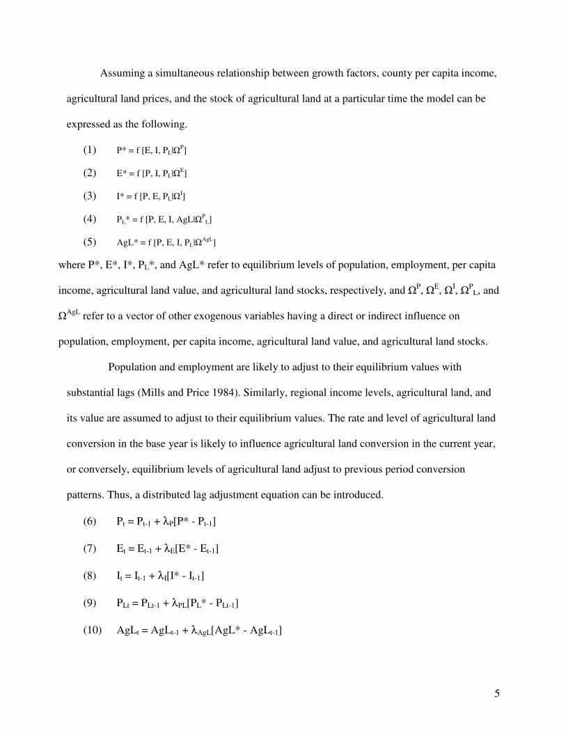
Assuming a simultaneous relationship between growth factors, county per capita income,
agricultural land prices, and the stock of agricultural land at a particular time the model can be
expressed as the following.
(1) P* = f [E, I, PL|�P]
(2) E* = f [P, I, PL|�E]
(3) I* = f [P, E, PL|�I]
(4) PL* = f [P, E, I, AgL|�PL]
(5) AgL* = f [P, E, I, PL|�AgL]
where P*, E*, I*, PL*, and AgL* refer to equilibrium levels of population, employment, per capita
income, agricultural land value, and agricultural land stocks, respectively, and �P, �E, �I, �PL, and
�AgL refer to a vector of other exogenous variables having a direct or indirect influence on
population, employment, per capita income, agricultural land value, and agricultural land stocks.
Population and employment are likely to adjust to their equilibrium values with
substantial lags (Mills and Price 1984). Similarly, regional income levels, agricultural land, and
its value are assumed to adjust to their equilibrium values. The rate and level of agricultural land
conversion in the base year is likely to influence agricultural land conversion in the current year,
or conversely, equilibrium levels of agricultural land adjust to previous period conversion
patterns. Thus, a distributed lag adjustment equation can be introduced.
(6) Pt = Pt-1 + λP[P* - Pt-1]
(7) Et = Et-1 + λE[E* - Et-1]
(8) It = It-1 + λI[I* - It-1]
(9) PLt = PLt-1 + λPL[PL* - PLt-1]
(10) AgLt = AgLt-1 + λAgL[AgL* - AgLt-1]
6
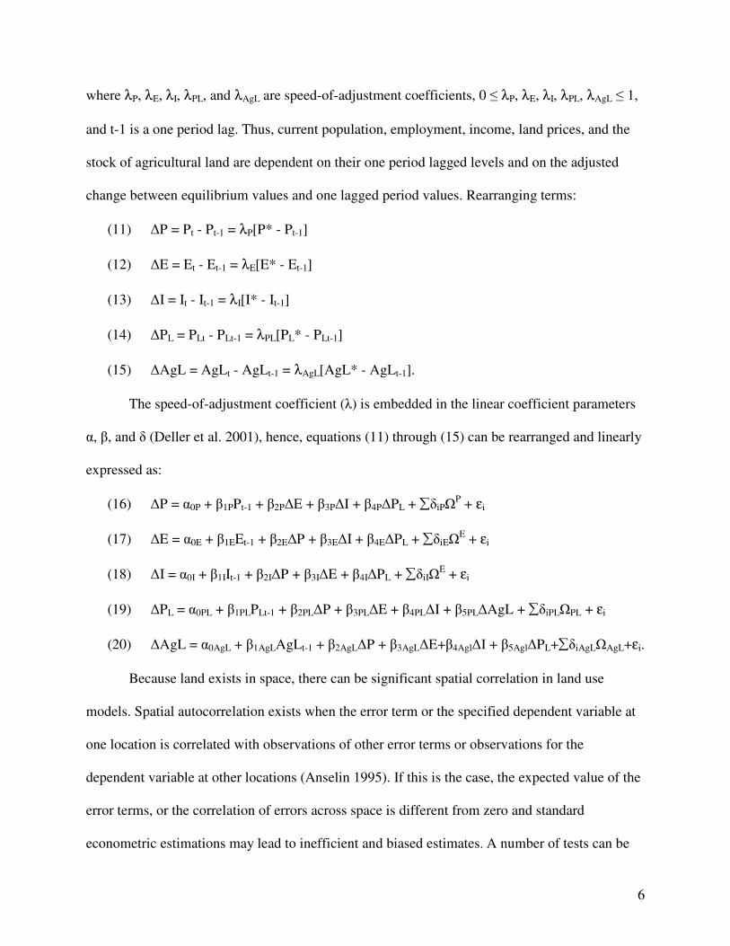
where λP, λE, λI, λPL, and λAgL are speed-of-adjustment coefficients, 0 � λP, λE, λI, λPL, λAgL � 1,
and t-1 is a one period lag. Thus, current population, employment, income, land prices, and the
stock of agricultural land are dependent on their one period lagged levels and on the adjusted
change between equilibrium values and one lagged period values. Rearranging terms:
(11) �P = Pt - Pt-1 = λP[P* - Pt-1]
(12) �E = Et - Et-1 = λE[E* - Et-1]
(13) �I = It - It-1 = λI[I* - It-1]
(14) �PL = PLt - PLt-1 = λPL[PL* - PLt-1]
(15) �AgL = AgLt - AgLt-1 = λAgL[AgL* - AgLt-1].
The speed-of-adjustment coefficient (�) is embedded in the linear coefficient parameters
�, �, and � (Deller et al. 2001), hence, equations (11) through (15) can be rearranged and linearly
expressed as:
(16) �P = �0P + �1PPt-1 + �2P�E + �3P�I + �4P�PL + ��iP�P + εi
(17) �E = �0E + �1EEt-1 + �2E�P + �3E�I + �4E�PL + ��iE�E + εi
(18) �I = �0I + �1IIt-1 + �2I�P + �3I�E + �4I�PL + ��iI�E + εi
(19) �PL = �0PL + �1PLPLt-1 + �2PL�P + �3PL�E + �4PL�I + �5PL�AgL + ��iPL�PL + εi
(20) �AgL = �0AgL + �1AgLAgLt-1 + �2AgL�P + �3AgL�E+�4Agl�I + �5Agl�PL+��iAgL�AgL+εi.
Because land exists in space, there can be significant spatial correlation in land use
models. Spatial autocorrelation exists when the error term or the specified dependent variable at
one location is correlated with observations of other error terms or observations for the
dependent variable at other locations (Anselin 1995). If this is the case, the expected value of the
error terms, or the correlation of errors across space is different from zero and standard
econometric estimations may lead to inefficient and biased estimates. A number of tests can be

7
used to discover whether the model should be a spatial lag or spatial error model. In this study,
appropriate spatial econometric tests and estimations are conducted on the reduced form
equations of the simultaneous system.
County level data for West Virginia, Maryland, and Pennsylvania for 1987, 1999, and
2002 are used to estimate the econometric models. The source for population, employment, per
capita income, and unemployment rate data is the Regional Economic Information Service
(REIS). Data on agricultural land value, agricultural land acreage, government financial
assistance to farmers, land conservation programs (CRP), proportion of total lands in farms,
agricultural income per farm and farm employment are generated from the U.S. Agricultural
Census. Per capita taxes, property taxes, government expenditures per capita, median housing
value, crime rate, number of physicians and education levels are from the County and City Data
Book. Growth variables and spatial data were computed from the above mentioned data sets.
Results and Discussion
Two empirical models are estimated in this study. The first uses a three-stage-least-
squares approach to simultaneously identify the impact of growth on agricultural lands. The
second model investigates possible spatial dependence in the data. Due to the complexity of
estimating such a simultaneous spatial econometric system, we identify reduced form equations
for the simultaneous system and estimate each equation using spatial lags to test for spatial
dependence. A complete list of variables and their definitions is provided in Table 1.
Estimation results from the first system of simultaneous equations are presented in Table
2. Population growth (∆P) is positively and significantly related with employment expansion
(∆E), asserting that in our study area people follow jobs. The relationship between population
growth and per capita income growth (∆PCI) is negative, suggesting that population growth is

8
higher in rural and suburban communities where income growth is slower. The significant and
negative relationship between population growth and agricultural land prices (∆AgLP) may be
due to high per acre land values discouraging housing development, and/or high farmland values
reflecting high productivity and less interest by farmers in selling their land for development.
Fiscal factors, local tax burden (PCTAXt-1) and property taxes (TAXPPROt-1), have the expected
negative effect on local population growth, as evidenced by estimated coefficients that are
negative and significant. This result is consistent with the theoretical expectation that people are
mobile across space to optimize tax burdens. A positive relationship between the crime rate
(CRIM100kt-1) and population growth was not expected, however, the effect of crime may have
been overshadowed by other local attributes that encourage population growth.
Employment growth (∆E) is positively and significantly related with population growth
(∆P), per capita income expansion (∆PCI), and land prices (∆AgLP). The expansion of
employment following population growth has been supported in previous studies. A growing
population provides the markets and labor pool that attract new businesses and employment.
Employment opportunities also expand in counties with growing per capita income and
purchasing power. The expansion of employment demands land that may come from farmland
development. If this pressure is significant, farmland prices would be expected to rise. These
results indicate that employment growth is higher in counties that are experiencing growth in
farmland prices. Mining is an important economic activity in our study area, and its contribution
to local employment and hence employment growth is significant. Our results show that there is
a significant contribution by the service sector to job growth (SERVEMPt-1), but construction
employment (CONSTEMPt-1) is negatively related to job growth. This could be a reflection of
slower overall employment growth in counties with high employment in construction jobs. Fiscal

9
characteristics of communities can be an important determinant of employment growth. Property
taxes (TAXPPRt-1), used to proxy the impact of taxes on job creation in the study area, are
significantly and negatively related with job growth, meeting prior expectations. Differences in
human capital endowments are hypothesized to lead to different job growth patterns. In our study
area, education levels (proportion of county 25 and above with high school or higher,
PERHIGDAt-1) are positively and significantly related to employment growth.
Per capita income growth (∆PCI) is significantly and negatively affected by population
growth (∆P), indicating for our study area that areas with lower population density experienced
larger income growth than dense population centers. This result confirms the decentralization of
jobs to suburbs and rural areas where population concentration is comparatively low. Income
growth is positively and significantly related with employment growth. Fiscal burdens, like per
capita income (PCTAXt-1) and property taxes (TAXPPROt-1) were expected to slow down income
growth, however, both variables were positively related to income growth. This may be due to
reinvestment of high tax revenues by counties through the provision of better public goods that
may partially offset the negative impacts of taxes. The effect of poverty on income growth, as
expected, indicates that counties with a high proportion of income levels below poverty
(PPOINCBPt-1) experienced slower income growth. Counties with high poverty rates are less
likely to attract new jobs and investment, consequently per capita income growth may be
hampered.
Increases in agricultural land prices (∆AgLP) not only affect the rate of agricultural land
development but also the distribution of population and employment growth (∆E) across space.
Our results show that higher agricultural land prices have a negative impact on population and
per capita income growth. The agricultural land price is significantly and positively influenced

10
by employment growth, indicating that growth in employment puts upward pressure on
agricultural land prices. However, the expectation that growth in population and income lead to
higher farmland prices is not supported by our analysis. Counties with higher farmland prices at
the beginning of the study period experienced positive growth in farmland prices as indicated by
a positive and significant coefficient on the initial period agricultural land prices (AgLPt-1). The
initial density of cropland (DCROPLt-1) has a negative coefficient, as expected, indicating that an
initial high endowment of cropland is associated with lower farmland prices. In other words,
increasing scarcity of farmland over time is likely to lead to higher farmland prices. Agricultural
land prices are also influenced by farmland productivity as measured by agricultural income per
farm (AGINCPFAt-1). For our study area, the results suggest that for every $1 increase in farm
income, the average value of farmland increases by $0.038 cents per acre. Thus, income support
to farmers is capitalized into higher farmland values, which in turn discourage population and
income growth in suburban and rural areas. A positive and significant relationship is found
between the amount of land in the Conservation Reserve Program (CRP) (LICONSRPt-1) and
farmland prices since land enrolled in the CRP is at least temporarily unavailable for
development.
Looking at agricultural land density, we find that high growth in population density (∆P)
is associated with high farmland losses (∆AgL) as agricultural land is developed. There is also a
positive relationship between farmland price growth (AgLP) and farmland development. With
development pressure, the value of farmland increases partly due to speculation. Thus, high
growth in farmland prices may indicate the extent of development pressure on farmland, after
accounting for its increase in the value due to productivity of the farm sector. Employment and
per capita income growth did not have a significant impact on agricultural land density. The
11
initial cropland density variable (DCROPLt-1) has a significant positive impact on agricultural
land levels, indicating that a large concentration of crop farming activity tends to reduce
development. This may be due to the nature of economic activities where concentrated large
scale farming brings economies of scale in input and output markets. More dense farming
activity is likely to challenge development compared to fragmented farmland due to collective
advantages and economies of scale. This may indicate that there could be a threshold of farmland
density below which farming activity becomes sensitive to development. Finally, government
financial assistance to farmers (GVPYPFARt-1) was significant in slowing down farmland
development. In the presence of many positive externalities to society from the agricultural
sector, the public may interfere in terms of policy support or direct financial assistance. These
results indicate that such government assistance programs have a significant impact in terms of
reducing farmland development.
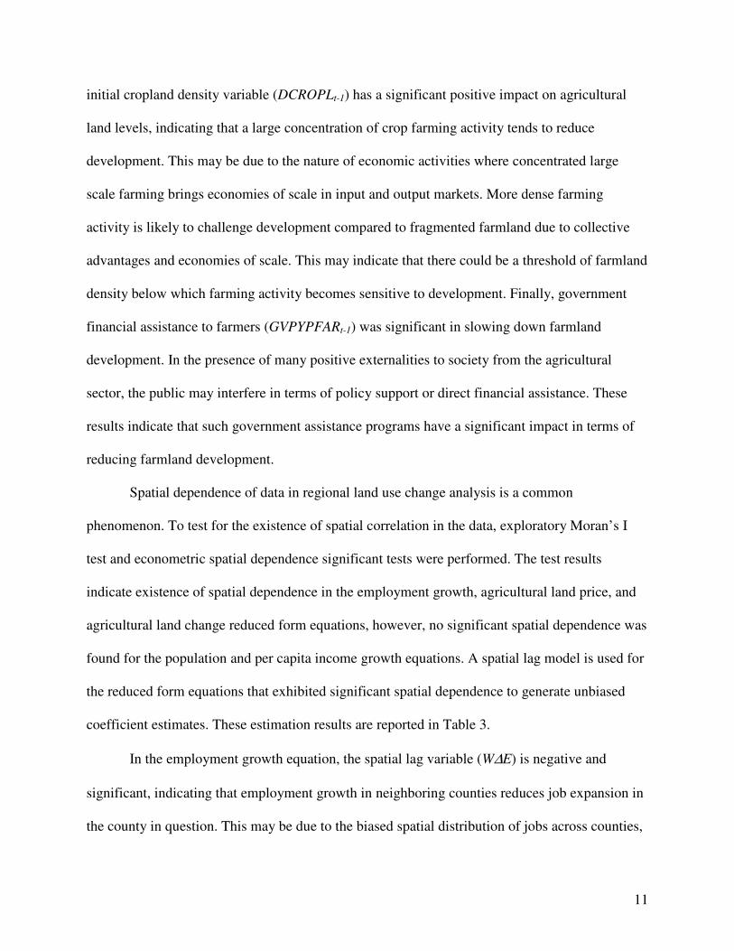
Spatial dependence of data in regional land use change analysis is a common
phenomenon. To test for the existence of spatial correlation in the data, exploratory Moran’s I
test and econometric spatial dependence significant tests were performed. The test results
indicate existence of spatial dependence in the employment growth, agricultural land price, and
agricultural land change reduced form equations, however, no significant spatial dependence was
found for the population and per capita income growth equations. A spatial lag model is used for
the reduced form equations that exhibited significant spatial dependence to generate unbiased
coefficient estimates. These estimation results are reported in Table 3.
In the employment growth equation, the spatial lag variable (W∆E) is negative and
significant, indicating that employment growth in neighboring counties reduces job expansion in
the county in question. This may be due to the biased spatial distribution of jobs across counties,

12
where counties with high employment growth attract commuters form neighboring counties,
creating further incentives for job creation at that destination. Similar to the conclusion reached
in the non-spatial system of equations model, this result indicates that employment growth is
positively related with population endowment and the initial income level of counties, along with
the level of human capital formation, while taxes, land conservation efforts, the crime rate, a
higher unemployment rate, and high housing values may slow employment growth.
The agricultural land price spatial lag variable (W∆AgLP) is positive and significant,
indicating that high farmland prices in neighboring counties put pressure on local farmland
prices due to increasing development pressure that is increasing speculation regarding future
development. After correcting for spatial correlation, farmland price growth is positively related
with initial population density, initial per capita income, and construction employment, which
may be due to an increased demand for land to accommodate a growing population base. A
positive relationship with higher farm income, on the other hand, means that a better return on
farmland is being translated into high farmland prices following Ricardian land rent theory.
Taxes and the crime rate are significantly and negatively related with farmland price growth.
Higher taxes and higher crime rates discourage population and employment relocation to these
locations resulting in lower demand for land and hence lower farmland prices.
Finally, the agricultural land change spatial lag variable (WAgL) has a positive and
significant relationship with change in agricultural land. This indicates that counties whose
neighbors are experiencing high levels of farmland development may also see development of
their farmlands as well. This suggests a sprawling pattern of development of farmland. The
performance of the spatial model is weak compared to the non-spatial system, however, the
results indicate that local externalities in terms of higher property values and unemployment are

13
related to lower farmland losses. Places with weaker employment performance and high property
values as well as those with higher crime rates or higher taxes may discourage migration of
population and employment creation, hence limiting the pressure on farmland developments.
Conclusion
This study provides a theoretical and empirical modeling approach to understanding
agricultural land development from a regional growth perspective. A simultaneous equilibrium
model is developed to estimate the interaction of endogenous variables of growth in population,
employment, per capita income, and agricultural land prices with agricultural land development.
Empirical three-stage-least-square estimation and spatial econometric estimation of reduced form
equations are undertaken.
The results suggest that while there is an array of factors that influence population
growth, from a farmland development perspective, population growth is negatively related with
increasing agricultural land prices. This may indicate that policies that increase farmland values
are likely to reduce population growth and pressure on farmland development. Employment
growth is also affected by a number of socio-economic conditions, however, from a farmland
development perspective, higher farmland prices were associated with employment growth,
suggesting that an increase in farmland prices may not reduce employment growth and pressure
on farmland development. Per capita income growth may indicate the level of economic activity
in a county and is positively related to employment growth. A negative relationship with
farmland prices indicates that counties with high farmland prices experienced lower per capita
income growth. From a policy perspective, government transfer programs that increase the value
of farmland may slow development and income growth. Agricultural land prices are positively
affected by employment growth, higher farm incomes, and land conservation. However, a higher

14
county endowment of agricultural lands tends to reduce the land market value of farmland. This
study also concludes that farmland stocks are negatively related to pressure from population
growth, however, no significant pressure on farmland stocks is found for employment and
income growth. High density farming activity and government farm financial assistance are
found to lessen pressure on farmland development. This may be due to economies of scale
associated with agglomerated farming activity and due to more net return in farming with
government assistance motivating farmers to keep their land in agriculture.
A spatial econometric approach is also used to correct for spatial correlation. Though
population and income growth have no significant spatial pattern, employment, farmland price,
and agricultural land change showed significant spatial dependence. While high employment
growth in neighboring counties slows employment growth in the local county, high farmland
prices and agricultural land development in neighboring counties results in higher farmland
prices and development in the local county. Understanding this spatial dependence in regional
growth and land use change is relevant for spatially explicit land use policies and management.

15
References
Abler, D. “Multifunctionality, Agricultural Policy, and Environmental Policy.” Paper presented
at the annual meeting of the Northeastern Agricultural and Resource Economics
Association, Portsmouth, NH, June 10, 2003.
Anselin, L. SpaceStat Version 1.80 User’s Guide. Regional Research Institute, West Virginia
University, 1995.
Batie, S.S. “The Multifunctional Attributes of Northeast Agriculture: A Research Agenda.”
Agricultural and Resource Economics Review. 32(2003):1-8.
Bell, K.P., and E.G. Irwin. “Spatially Explicit Micro-level Modeling of Land Use Change at the
Rural-urban Interface.” Agricultural Economics. 27(2002):217-232.
Bowker, J.M., and D.D. Didychuk. “Estimation of the Nonmarket Benefits of Agricultural Land
Retention in Eastern Canada.” Agricultural and Resource Economics Review.
23(1994):218-225.
Brueckner, J.K., and D.A. Fansler. “The Economics of Urban Sprawl: Theory and Evidence on
the Spatial Sizes of Cities.” The Review of Economics and Statistics. 65(1983):479–482.
Burchell, R.W., and N.A. Shad. The Costs of Sprawl – Revisited. Transportation Research Board,
National Research Council. National Academy Press, Washington, D.C., 1998.
Carlino, G.A., and E.S. Mills. “The Determinants of County Growth.” Journal of Regional
Science. 27(1987):39-54.
Chandra, A., and E. Thompson. “Does Public Infrastructure Affect Economic Activity? Evidence
from the Rural Interstate Highway System.” Regional Science and Urban Economics.
30(2000):457-490.

16
Deller, S.C., T.-H. Tsai, D.W. Marcouiller, and D.B.K. English. “The Role of Amenities and
Quality of Life in Rural Economic Growth.” American Journal of Agricultural
Economics. 83(2001):352-365.
Dissart, J.C., and S.C. Deller. “Quality of Life in the Planning Literature.” Journal of Planning
Literature. 15(2000):135-161.
English, D.B.K, D.W. Marcouiller, and H.K. Cordell. “Linking Local Amenities with Rural
Tourism Incidence: Estimates and Effects.” Natural Resources. 13(2000):185-202.
Garcia-Mila, T. and T.J. McGuire. “The Contribution of Publicly Provided Inputs to States’
Economies.” Regional Science and Urban Economics. 22(1992):229-241.
Gottlieb, P.D. “Amenities as an Economic Development Tool: Is there Enough Evidence?” Econ.
Dev. Quart. 8(1994):270-85.
Heimlich, R.E., and W.D. Anderson. Development at the Urban Fringe and Beyond: Impacts on
Agriculture and Rural Land. Economic Research Service, U.S. Department of Agriculture.
Agricultural Economic Report No. 803, 2001.
Henry, M.S., D.L. Barkley, and S. Bao “The Hinterland’s Stake in Metropolitan Growth:
Evidence from Selected Southern Regions.” Jour. of Reg. Sci. 37(1997):479-501.
Irwin, E.G., and N.E. Bockstael. “Interacting Agents, Spatial Externalities, and the Endogenous
Evolution of Residential Land Use Patterns.” Ohio State University, Department of
Agricultural, Environmental, and Development Economics, Working Paper AEDE-WP-
0010-01, 2001.
Keeler, J.E., and J.S. Ying. “Measuring the Benefit of a Large Public Investment: the Case of the
US Federal-aid Highway System.” Jour. of Pub. Econ. 36(1988):69-85.

17
Kline, J., and D. Wichelns. “Public Preferences Regarding the Goals of Farmland Preservation
Programs.” Land Econ. 72(1996):538-49.
Lewis, D.J., G.L. Hunt, and A.J. Plantinga. “Public Conservation Land and Employment Growth
in the Northern Forest Region.” Land Econ. 78(2002):245-259.
Mieszkowski, P., and E.S. Mills. “The Causes of Metropolitan Suburbanization.” The Journal of
Economic Perspectives. 7(1993):135-147.
Mills, E.S., and R. Price. “Metropolitan Suburbanization and Central City Problems.” Journal of
Urban Economics. 15(1984):1-17.
Nickerson, C.J., and D. Hellerstein. “Protecting Rural Amenities through Farmland Preservation
Programs.” Agricultural and Resource Economics Review. 32(2003):129-144.
Northeast Regional Center for Rural Development (NERCRD). Land Use Problems and
Conflicts in the U.S., Research Workshop on Land Use Problems and Conflicts, Orlando,
FL., Feb. 21-22, 2002.
Plantinga, A.J., and D.J. Miller. “Agricultural Land Values and the Value of Rights to Future
Land Development.” Land Econ. 77(2001):56-67.
Porter, D. Managing Growth in America’s Communities. Island Press, Washington, D.C., 1997.
Power, T.M. Lost Landscapes and Failed Economies: The Search for a Value of Place. Island
Press. Washington, D.C., 1996.
Ready, R.C., M.C. Berger, and G.C. Blomquist. 1997. Measuring Amenity Benefits from
Farmland: Hedonic Pricing vs. Contingent Valuation. Growth and Change. 28:438-458.
Roback, J. “Wages, Rents, and Amenities: Differences Among Workers and Regions.” Economic
Inquiry. 26(1988):23-41.

18
Rosenberger, R.S., and J.B. Loomis. “The Value of Ranch Open Space to Tourists: Combining
Contingent and Observed Behavior Data.” Growth and Change. 30(1999):366-383.
Rosenberger, R.S., and R.G. Walsh. “Nonmarket Value of Western Valley Ranch Land Using
Contingent Valuation.” Journal of Agricultural and Resource Economics. 22(1997):296-
309.

19
Table 1. Variable Definitions.
∆P Population density change (1987-1999) ∆E Employment density change (1987-1999) ∆AgL Agricultural land density change (1987-2002) ∆PCI Change in per capita income (1987-1999) ∆AgLP Change in agricultural land price (1987-2002) DPOPt-1 Population density 1987 DEMPt-1 Employment density 1987 DAgLt-1 Agricultural land density 1987 PCIt-1 Per capita income 1987 AgLPt-1 Value of farmland per acre 1987 DCROPLt-1 Cropland density 1987 FARMEMPt-1 Farm employment 1987 SERVEMPt-1 Service employment 1987 MINEMPt-1 Mining employment 1987 CONSTEMPt-1 Construction employment 1987 PCTAXt-1 Per capita tax 1987 TAXPPROt-1 Percentage property tax 1987 AGINCPFAt-1 Agricultural income per farm 1987 GVPYPFARt-1 Government payments per farm 1987 OWNOCCHt-1 Owner occupied housing (percent of total) 1990 MEDHVALt-1 Median housing value 1990 UNEMPRTt-1 Unemployment rate 1990 PASTACRt-1 Pastureland acres 1987 PTLNDIFRt-1 Percentage of total land in farming 1987 LICONSRPt-1 Land in the Conservation Reserve Program 1987 CRIM100kt-1 Crime rate per 100,000 population 1990 PHYP100kt-1 Physicians per 100,000 population 1990 PERHIGDAt-1 Percentage of population with high school education and above 1990 PPOINCBPt-1 Percentage of population with income below poverty line 1990 GVEXPCAPt-1 Government expenditures per capita 1987 W∆E Spatial lag of employment growth (1987-1999) W∆AgLP Spatial lag of agricultural land price growth (1987-2002) W∆AgL Spatial lag of agricultural land change (1987-2002)

20
Table 2. First Equation System Econometric Results
∆∆∆∆P Equation ∆∆∆∆E Equation ∆∆∆∆PCI Equation ∆∆∆∆AgLP Equation ∆∆∆∆AgL Equation VARIABLE
Coef. p-value
Coef. p- value
Coef. p- value
Coef. p-value
Coef. p- value
Endogenous Variables
∆P - - 0.64* 0.00 -13.64* 0.00 -3.64 0.53 0.11§ 0.07
∆E 1.28* 0.00 - - 26.72* 0.00 26.16* 0.00 -0.104 0.36
∆PCI -0.02* 0.00 0.01* 0.01 - - -0.47§ 0.09 -0.002 0.36
∆AgLP -0.01* 0.00 0.02* 0.00 -0.25† 0.04 - - 0.01
† 0.03
∆AgL - - - - - - -6.07 0.78 - -
Initial Condition Variables
DPOPt-1 -0.05* 0.00 - - - - - - - -
DEMPt-1 - - -0.01 0.70 - - - - - -
PCIt-1 - - - - -0.29† 0.04 - - 0.001 0.77
AgLPt-1 - - - - - - 1.27* 0.00 - -
DAgLt-1 - - - - - - - - 0.59§ 0.05
DCROPLt-1 - - - - - - -48.63† 0.05 -0.69
§ 0.07
Exogenous Variables
FARMEMPt-1 - - - - - - 0.01 0.12
SERVEMPt-1 - - 0.01† 0.05 - - - - - -
MINEMPt-1 - - 0.02§ 0.09 - - - - - -
CONSTEMPt-1 - - -0.01§ 0.07 - - - - - -
PCTAXt-1 -0.06* 0.02 - - 5.92† 0.01 - - - -
TAXPPROt-1 -0.59 0.17 -1.18 0.01 48.96* 0.00 - - -0.31 0.31
AGINCPFAt-1 - - - - - - 0.04† 0.02 0.001 0.77
GVPYPFARt-1 - - - - - - - - -0.01† 0.02
OWNOCCHt-1 5.48† 0.04 - - - - - - - -
MEDHVALt-1 0.001* 0.00 - - - - - - - -
UNEMPRTt-1 - - -11.27† 0.02 463.7* 0.00 - - - -
PASTACRt-1 - - - - - - - - -0.001† 0.05
PTLNDIFRt-1 - - - - - - 141.19§ 0.09 - -
LICONSRPt-1 - - - - - - 5.50§ 0.05 - -
CRIM100kt-1 0.01† 0.05 - - - - - - - -
PHYP100kt-1 -0.10* 0.01 - - - - - - - -
PERHIGDAt-1 - - 1.47§ 0.10 - - - - - -
PPOINCBPt-1 - - 9.54* 0.01 -399.1* 0.00 - - - -
GVEXPCAPt-1 - - - - -3743.4* 0.00 - - - -
Constant -349.12 0.04 -137.46 0.06 8474.1 0.001 116.68 0.89 31.87 0.31
Note: § indicates statistical significance at the 10% level, † indicates significance at 5%, and * indicates significant at the 1% level.
21
Table 3. Spatial Equation System Econometric Results
∆∆∆∆E Equation ∆∆∆∆AglP Equation ∆∆∆∆Agl Equation VARIABLE
Coefficient p -Value Coefficient p -Value Coefficient p -Value Spatial-lag Variables
W∆E -0.1341† 0.045 - - - -
W∆AgLP - - 0.642* 0.000 - - WAgL - - - - 0.363* 0.0002 Initial Condition Variables DPOPt-1 0.051 0.122 4.712* 0.000 0.031 0.284 DEMPt-1 -0.295* 0.000 -8.896* 0.000 0.048 0.328 PCIt-1 0.010* 0.000 0.100 0.187 -0.0003 0.901 AgLPt-1 0.031* 0.000 0.473§ 0.077 0.006 0.432 DAgLt-1 0.908* 0.000 5.908 0.375 -0.629* 0.0005 DCROPLt-1 -0.315* 0.000 -4.155 0.157 -0.036 0.655 Exogenous Variables FARMEMPt-1 -0.011* 0.000 -0.242† 0.004 0.001 0.596 SERVEMPt-1 0.0001 0.382 -0.018† 0.013 -0.0002 0.383 CONSTEMPt-1 0.006* 0.000 0.178* 0.000 0.001 0.431 PCTAXt-1 -0.035§ 0.087 -1.831* 0.004 0.037† 0.037 AGINCPFAt-1 0.00004 0.959 0.011* 0.000 -0.00007 0.292 OWNOCCHt-1 -0.394 0.765 24.316 0.228 0.042 0.939 MEDHVALt-1 -0.0001 0.452 -0.009 0.165 -0.0004† 0.017 UNEMPRTt-1 -0.394 0.765 -47.674 0.253 -2.129§ 0.062 PTLNDIFRt-1 -4.349* 0.0001 -30.774 0.465 4.232* 0.0002 LICONSRPt-1 -0.014† 0.014 0.052 0.777 -0.00009 0.984 CRIM100kt-1 -0.002 0.328 -0.146§ 0.062 -0.0005 0.814 PHYP100kt-1 0.013 0.301 0.616 0.118 -0.013 0.218 PERHIGDAt-1 1.102† 0.038 31.265§ 0.063 0.181 0.697 PPOINCBPt-1 2.614* 0.004 50.090§ 0.074 0.941 0.225 Constant -211.099 0.007 -4620.803 0.062 4.729 0.0002 Likelihood Ratio Value = 3.471
p-Value = 0.062 Value = 42.131 p-Value = 0.000
Value = 12.253 p-Value = 0.0004
Note: the sign § indicates statistical significance at 10%, † indicates significance at 5%, and * indicates significant at 1% level.