ecofys netherlands bv - aaee

Global technical potentials for energy efficiency improvement Wina Graus, Eliane Blomen, Corinna Kleßmann, Carolin Capone, Eva Stricker

Ecofys Netherlands bv

Presented at IAEE European Conference September 2009

Abstract

In this study the technical potential and costs are calculated for global energy efficiency improvement in 2050 based on literature sources. The reference scenario is based on the World Energy Outlook (WEO) of the International Energy Agency edition 2007 (IEA, 2007a) and assumptions regarding GDP development after 2030. The results of this study are that on a business-as-usual trajectory, worldwide final energy demand grows by 95% from 290 EJ in 2005 to 570 EJ in 2050. By exploiting the technical potential for energy efficiency improvement in that period the increase can be limited to 8% or 317 EJ in 2050. It is estimated that to implement the global technical potential, annual costs equivalent to 0.5% of GDP in 2050 are needed. It was found that there is a large potential for cost-effective measures, equivalent to around 55-60% of energy savings of the efficiency measures.

1 Introduction

Energy efficiency improvement potentials are key inputs into long term energy and greenhouse gas emission scenarios (e.g. IEA WEO 2007 Alternative Policy Scenario (APS), The Blue Map Scenario of IEA ETP 2008 and the Greenpeace/EREC energy [r]evolution scenario). In spite of the acknowledged large potential, few reports are available on the potential and especially on related costs of energy efficiency improvement, in a global context. There are a number of studies focusing on costs of greenhouse gas abatement, such as McKinsey (2007), in which energy efficiency measures are part of the measures evaluated. Another example is the Stern Review (Stern et al., 2006), where the annual costs of combating global warming are estimated to amounting to €2 trillion (to avoid €9 trillion in annual damage), corresponding to around 3.5% of expected GDP in 2050. Their message is that the costs of stabilising the climate are significant but manageable; delay would be dangerous and much more costly.

In this study a scenario is developed up to 2050, where technical potentials and costs for energy efficiency improvement are calculated, based on available literature sources.

This paper is structured as follows. First the approach and data sources are described in section 2 followed by the results in section 3. Section 4 gives a discussion of uncertainties and section 5, lastly presents conclusions.

2 Approach and data sources

This study focuses on final energy demand, meaning that losses in energy transformation are not included. In 2005 global final energy demand equals 293 EJ and primary energy supply equals 432 EJ. This implies a conversion efficiency (ratio of final energy demand and primary energy demand) of 68%.

The potentials for energy efficiency improvement are calculated relative to a reference scenario, where current trends continue and no large changes take place in the production and consumption structure of the current economy. The reference scenario is based on the World Energy Outlook (WEO) of the

International Energy Agency edition 2007 (IEA, 2007a), for the period 2005-2030. For the period 2030-2050 the WEO scenario is extended by GDP forecasts from Simon et al. (2008). Under the reference scenario global GDP grows by 440% from 63,720 bln US$ (in 2006 dollars, PPP) in 2005 to 279,100 bln US$ in 2050. Population increases from 6.5 billion in 2005 to 9.2 billion in 2050. The economic growth assumptions are summarised in Table 1.

The regional disaggregation in this study is the same as the one used in the WEO 2007 edition; OECD Europe, OECD North America, OECD Pacific, Transition Economies, China, India, Rest of developing Asia, Latin America, Africa and Middle East (see IEA, 2007a).

Table 1: GDP development projections (average annual growth rates) (2010-2030: IEA (2007a) and

2030-2050: Simon et al. (2008))

2010 2015 2020 2030 2040 2050

OECD Europe 2.6% 2.2% 2.0% 1.7% 1.3% 1.1%OECD North America 2.7% 2.6% 2.3% 2.2% 2.0% 1.8%OECD Pacific 2.5% 1.9% 1.7% 1.5% 1.3% 1.2%Transition Economies 5.6% 3.8% 3.3% 2.7% 2.5% 2.4%India 8.0% 6.4% 5.9% 5.7% 5.4% 5.0%China 9.2% 6.2% 5.1% 4.7% 4.2% 3.6%Rest of Developing Asia 5.1% 4.1% 3.6% 3.1% 2.7% 2.4%Latin America 4.3% 3.3% 3.0% 2.8% 2.6% 2.4%Africa 5.0% 4.0% 3.8% 3.5% 3.2% 3.0%Middle East 5.1% 4.6% 3.7% 3.2% 2.9% 2.6%World 4.6% 3.8% 3.4% 3.2% 3.0% 2.9%

The growth of energy demand as a result of GDP growth depends on the development the “energy intensity” of the economy. Energy intensity is in this study defined as final energy use per unit of gross domestic product. The energy intensity in an economy tends to decrease over time. Energy intensity decrease can be a result of a number of factors e.g.:

� Autonomous energy efficiency improvement. These energy efficiency improvements occur because due to technological developments each new generation of capital goods is likely to be more energy efficient than the one before. This is mainly caused by (temporary) increases in energy prices, which leads economic actors to try to save energy e.g. by investing in energy efficiency measures or changing their behaviour.

� Policy-induced energy efficiency improvement as a result of which economic actors change their behaviour and invest in more energy efficient technologies.

� Decoupling of economic growth and energy use. A decline of the ratio of energy over GDP ratio is not caused only by energy efficiency improvement (that includes technical changes and operational improvements). In addition, structural changes can have a downward effect on the energy over GDP ratio. E.g. a shift in the economy away from energy-intensive industrial activities to services related activities. Also there may be demand saturation. E.g. energy use for heating tends to grow in proportion to floor surface rather than in proportion to economic growth.

The energy intensity decrease in the reference scenario results from a mix of these factors and differs per region and per sector. For the period 2005-2030 the energy intensity decrease results directly from the WEO 2007. For the period 2030-2040 and the period 2040-2050 the energy intensity decrease (as % per year) is based on the development of the energy intensity per region and sector in the period 2020-2030 in WEO. The energy intensity in the period 2005-2050 decreases from 4.6 MJ/US$ to 2.0 MJ/US$ (or 1.8% per year).

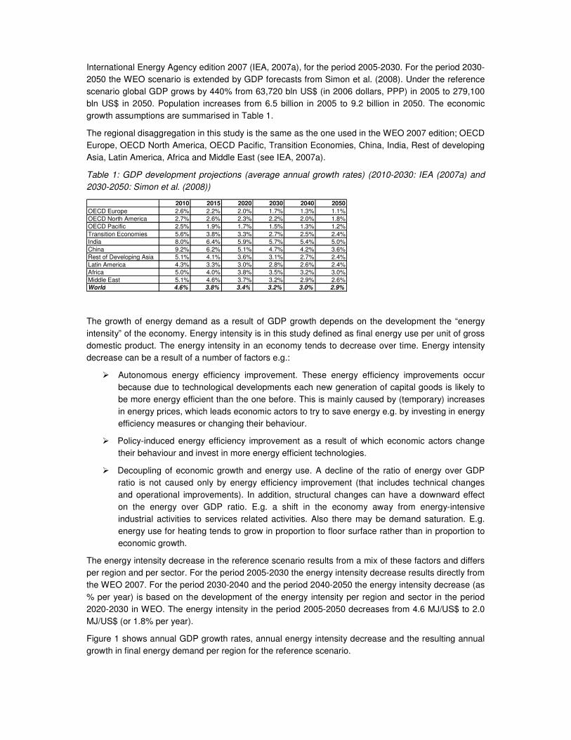
Figure 1 shows annual GDP growth rates, annual energy intensity decrease and the resulting annual growth in final energy demand per region for the reference scenario.

-3.0%

-2.0%

-1.0%

0.0%

1.0%

2.0%

3.0%

4.0%

5.0%

6.0%

7.0%

World

OECD P

acific

OECD E

urop

e

OECD Nor

th A

mer

ica

Latin

Am

erica

Trans

ition e

cono

mies

Rest o

f dev

eloping

Asia

Midd

le East

Africa

China

India

GDP growth rate

Energy-intensity

Growth final energy demand

Figure 1: Growth final energy demand in average % per year in period 2005-2050

The figure shows that final energy demand is projected to increase most in India and China (3.2%/y and 2.4%/y, respectively), followed by Middle East (2.2%/y) and Latin America (2.0%/y). Energy demand increase is lowest in OECD Europe, OECD Pacific and OECD North America (between 0.6%/y and 0.9%/y), due to lower GDP growth rates.

The reference scenario covers energy demand development for three sectors; (1) transport, (2) industry and (3) others (i.e. buildings and agriculture). Per sector a distinction is made between (1) electricity demand and (2) fuel and heat demand. Fuel and heat demand is shortly referred to as fuel demand. The energy demand scenario focuses only on energy-related fuel, power and heat use. This means that feedstock consumption in industries is excluded. This is done by assuming that the share of feedstock use in total energy use in industry remains the same as in the base year 2005.

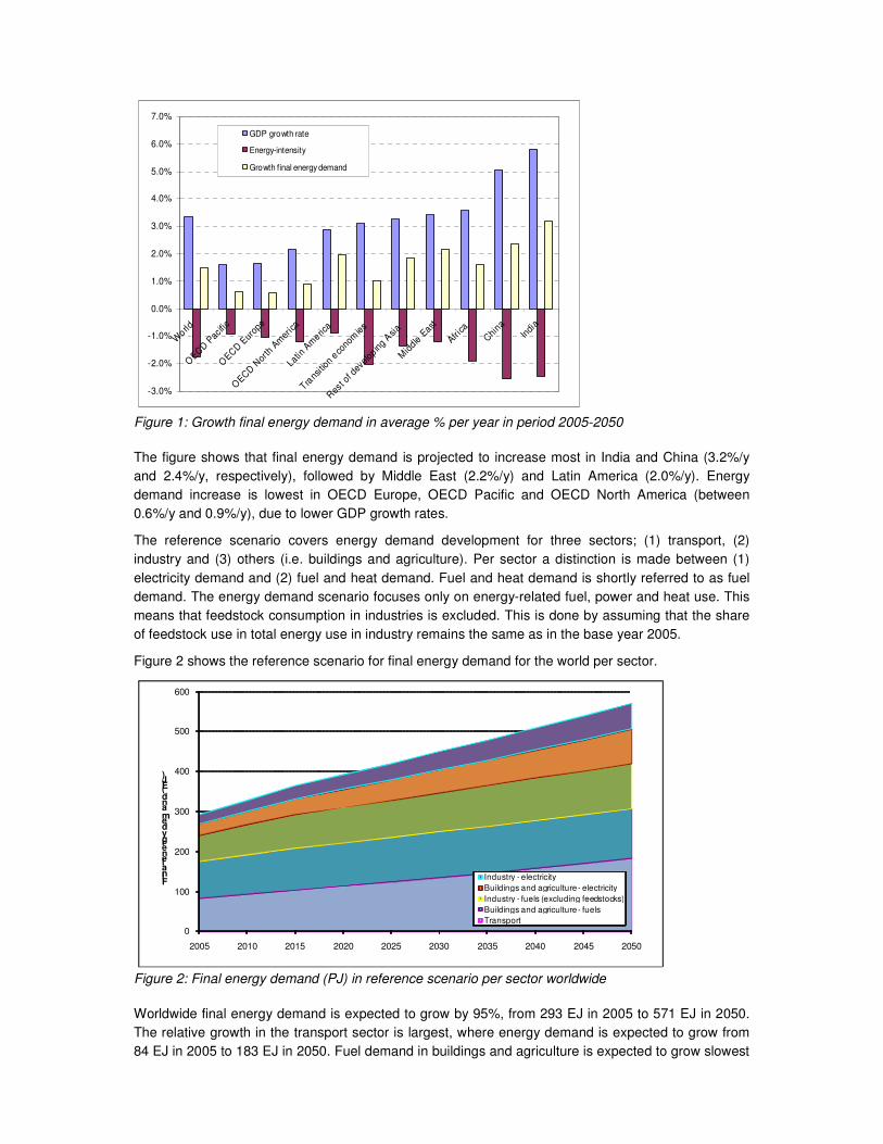
Figure 2 shows the reference scenario for final energy demand for the world per sector.

0

100

200

300

400

500

600

2005 2010 2015 2020 2025 2030 2035 2040 2045 2050

Final energy demand (EJ)

Industry - electricityBuildings and agriculture - electricityIndustry - fuels (excluding feedstocks)Buildings and agriculture - fuelsTransport

Figure 2: Final energy demand (PJ) in reference scenario per sector worldwide

Worldwide final energy demand is expected to grow by 95%, from 293 EJ in 2005 to 571 EJ in 2050. The relative growth in the transport sector is largest, where energy demand is expected to grow from 84 EJ in 2005 to 183 EJ in 2050. Fuel demand in buildings and agriculture is expected to grow slowest

from 91 EJ in 2005 to 124 EJ in 2050.

In the reference scenario, final energy demand in 2050 will be largest in China (121 EJ), followed by OECD North America (107 EJ) and OECD Europe (68 EJ). Final energy demand in OECD Pacific and Middle East will be lowest (28 EJ and 31 EJ respectively).

In terms of final energy demand per capita, there are still large differences between world regions in 2050. Energy demand per capita is expected to be highest in OECD North America (186 GJ/capita), followed by OECD Pacific and Transition Economies (156 respectively 142 GJ/capita). Final energy demand in Africa, India, Latin America, and Rest of developing Asia is expected to be lowest, ranging from 19-58 GJ/capita.

2.1 Technical potentials

The technical potentials for energy efficiency improvement are calculated on basis of literature sources. The potentials incorporate technical measures and do not include energy savings potentials by behavioural or organisational changes, or different economic structures. Besides current best practices also emerging technologies are taken into account in estimating potentials for energy efficiency improvement as well as improved material efficiency. We assume that measures can be implemented after 2010 and that equipment is replaced at the end of lifetime.

For the calculation of the technical potentials it is important to know the share of energy intensity decrease in the reference scenario as a result of energy efficiency improvement and the share of energy intensity decrease as a result of other factors (decoupling of economic growth, structural shifts). This in order to determine the share of the technical potential that is already implemented in the reference scenario. Energy efficiency improvement is defined as the decrease in specific energy consumption per physical unit (e.g. GJ/tonne crude steel, MJ/passenger km, MJ/m2 floor surface etc.). The energy intensity decrease in the reference scenario differs per region, ranging from 1 to 2.5%/year. The share of this, which is due to energy efficiency improvement, is unknown. We therefore assume that the energy efficiency improvement is equal to 1% per year for all regions, based on historical developments of energy efficiency (see e.g. Ecofys (2001), Blok (2005), Odyssee (2005)).

The potentials are per sector; transport, industry and others.

2.1.1 Transport

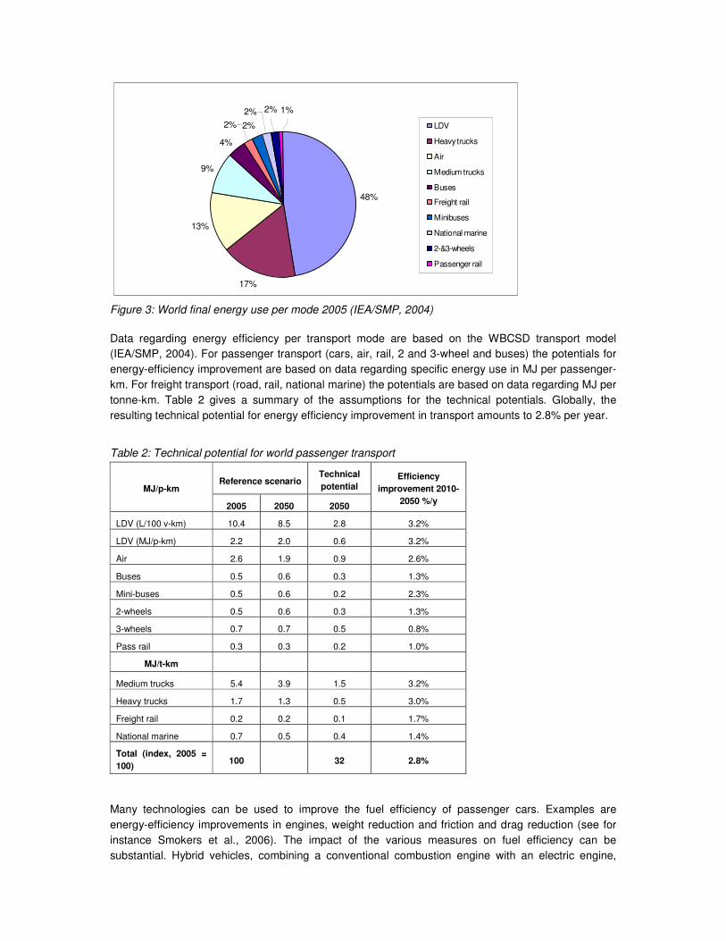
Worldwide, transport accounts for nearly 30% of final energy demand. For most regions the share of transport in energy demand is expected to increase by 2050. Especially developing regions show a sharp increase from 12-15% for India, China and Africa in 2005 to 26-30% in 2050. Please note that international marine shipping is not included in this study, due to lack of disaggregated data. Energy use from international marine shipping amounts to 9% of worldwide transport energy demand in 2005 and 7% in 2050.

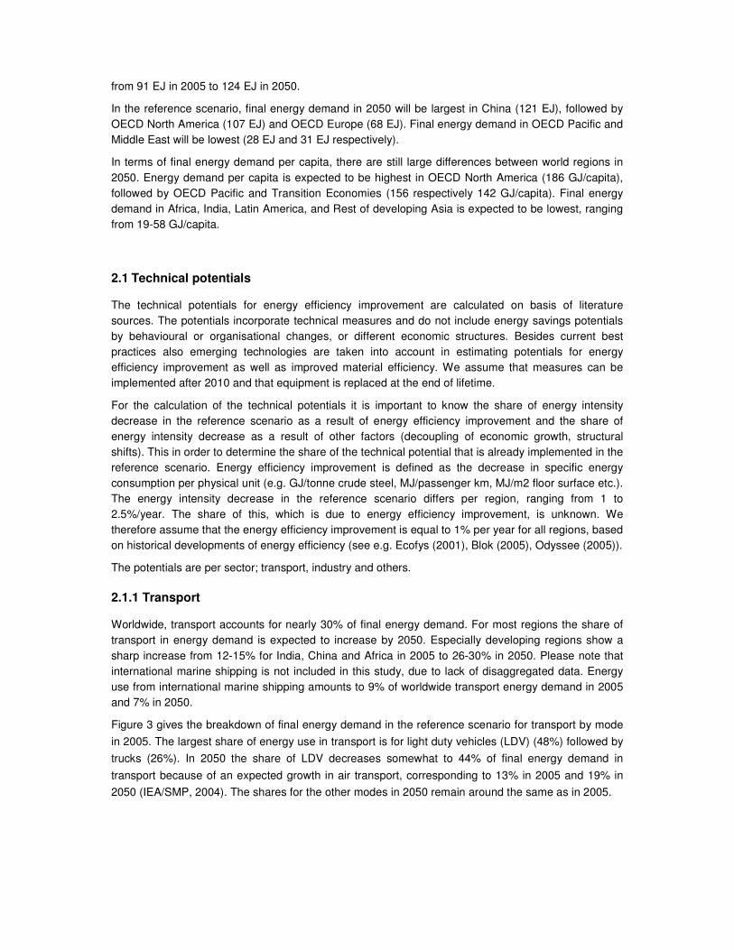
Figure 3 gives the breakdown of final energy demand in the reference scenario for transport by mode

in 2005. The largest share of energy use in transport is for light duty vehicles (LDV) (48%) followed by

trucks (26%). In 2050 the share of LDV decreases somewhat to 44% of final energy demand in

transport because of an expected growth in air transport, corresponding to 13% in 2005 and 19% in

2050 (IEA/SMP, 2004). The shares for the other modes in 2050 remain around the same as in 2005.

48%

17%

13%

9%

2%

1%2%2%

2%

4%

LDV

Heavy trucks

Air

Medium trucks

Buses

Freight rail

Minibuses

National marine

2-&3-wheels

Passenger rail

Figure 3: World final energy use per mode 2005 (IEA/SMP, 2004)

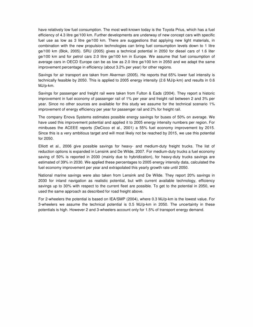
Data regarding energy efficiency per transport mode are based on the WBCSD transport model (IEA/SMP, 2004). For passenger transport (cars, air, rail, 2 and 3-wheel and buses) the potentials for energy-efficiency improvement are based on data regarding specific energy use in MJ per passenger-km. For freight transport (road, rail, national marine) the potentials are based on data regarding MJ per tonne-km. Table 2 gives a summary of the assumptions for the technical potentials. Globally, the resulting technical potential for energy efficiency improvement in transport amounts to 2.8% per year.

Table 2: Technical potential for world passenger transport

Reference scenario Technical

potential MJ/p-km

2005 2050 2050

Efficiency

improvement 2010-

2050 %/y

LDV (L/100 v-km) 10.4 8.5 2.8 3.2%

LDV (MJ/p-km) 2.2 2.0 0.6 3.2%

Air 2.6 1.9 0.9 2.6%

Buses 0.5 0.6 0.3 1.3%

Mini-buses 0.5 0.6 0.2 2.3%

2-wheels 0.5 0.6 0.3 1.3%

3-wheels 0.7 0.7 0.5 0.8%

Pass rail 0.3 0.3 0.2 1.0%

MJ/t-km

Medium trucks 5.4 3.9 1.5 3.2%

Heavy trucks 1.7 1.3 0.5 3.0%

Freight rail 0.2 0.2 0.1 1.7%

National marine 0.7 0.5 0.4 1.4%

Total (index, 2005 =

100) 100 32 2.8%

Many technologies can be used to improve the fuel efficiency of passenger cars. Examples are energy-efficiency improvements in engines, weight reduction and friction and drag reduction (see for instance Smokers et al., 2006). The impact of the various measures on fuel efficiency can be substantial. Hybrid vehicles, combining a conventional combustion engine with an electric engine,

have relatively low fuel consumption. The most well-known today is the Toyota Prius, which has a fuel efficiency of 4.3 litre ge/100 km. Further developments are underway of new concept cars with specific fuel use as low as 3 litre ge/100 km. There are suggestions that applying new light materials, in combination with the new propulsion technologies can bring fuel consumption levels down to 1 litre ge/100 km (Blok, 2005). SRU (2005) gives a technical potential in 2050 for diesel cars of 1.6 liter ge/100 km and for petrol cars 2.0 litre ge/100 km in Europe. We assume that fuel consumption of average cars in OECD Europe can be as low as 2.0 litre ge/100 km in 2050 and we adapt the same improvement percentage in efficiency (about 3.2% per year) for other regions.

Savings for air transport are taken from Akerman (2005). He reports that 65% lower fuel intensity is technically feasible by 2050. This is applied to 2005 energy intensity (2.6 MJ/p-km) and results in 0.6 MJ/p-km.

Savings for passenger and freight rail were taken from Fulton & Eads (2004). They report a historic improvement in fuel economy of passenger rail of 1% per year and freight rail between 2 and 3% per year. Since no other sources are available for this study we assume for the technical scenario 1% improvement of energy efficiency per year for passenger rail and 2% for freight rail.

The company Enova Systems estimates possible energy savings for buses of 50% on average. We have used this improvement potential and applied it to 2005 energy intensity numbers per region. For minibuses the ACEEE reports (DeCicco et al., 2001) a 55% fuel economy improvement by 2015. Since this is a very ambitious target and will most likely not be reached by 2015, we use this potential for 2050.

Elliott et al., 2006 give possible savings for heavy- and medium-duty freight trucks. The list of reduction options is expanded in Lensink and De Wilde, 2007. For medium-duty trucks a fuel economy saving of 50% is reported in 2030 (mainly due to hybridization), for heavy-duty trucks savings are estimated of 39% in 2030. We applied these percentages to 2005 energy intensity data, calculated the fuel economy improvement per year and extrapolated this yearly growth rate until 2050.

National marine savings were also taken from Lensink and De Wilde. They report 20% savings in 2030 for inland navigation as realistic potential, but with current available technology, efficiency savings up to 30% with respect to the current fleet are possible. To get to the potential in 2050, we used the same approach as described for road freight above.

For 2-wheelers the potential is based on IEA/SMP (2004), where 0.3 MJ/p-km is the lowest value. For 3-wheelers we assume the technical potential is 0.5 MJ/p-km in 2050. The uncertainty in these potentials is high. However 2 and 3-wheelers account only for 1.5% of transport energy demand.

2.1.2 Industry

The worldwide average share of industry in total final energy demand is about 30%. The share in Africa is lowest with 16% in 2050. The share in China is highest with 43% in 2050. For the industry sector, technical potentials for energy efficiency improvement are based on (1) implementing best practice technology and emerging technologies, and (2) increased material efficiency (including recycling).

IEA (2008) estimates an average potential of 19-32% by implementing best available techniques (BAT) globally and an additional potential of 20-30% for new technologies. Together this amounts to a potential of 45% for implementing BAT and emerging technologies. We use this potential in our calculations. In order to illustrate the potential of best practice and emerging technologies in industry, we give a couple of examples for a few energy-intensive industrial processes: cement production, ammonia production, chlorine production and aluminium production.

• Cement production: Two important processes in producing cement are clinker production and the blending of clinker with additives to produce cement. Clinker production is the most energy intensive step in cement production. The current state of the art kilns consume 3.0 GJ/tonne clinker. The thermodynamic minimum is 1.8 GJ/tonne clinker, but strongly depends on the moisture content. The global average specific energy consumption per tonne clinker equals 4.2 GJ per tonne (based on REEEP, 2008). Based on current state of the art this implies a savings potential of 30%.

• Ammonia production: Ammonia production consumed more energy than any other process in the chemical industry and accounted for 18 percent of the energy consumed in this sector. Ammonia is mainly applied as a feedstock for fertilizer production. Current best practice energy intensity (excluding feedstock) is 8 GJ/tonne ammonia1 (Sinton et al, 2002). Average energy use for ammonia production in 2005 is equivalent to 15 GJ//tonne2 NH3 (REEEP, 2008). This corresponds to an average savings potential of 45% based on current best practice technology.

• Chlorine production: Chlorine production is the main electricity consuming process in the chemical industry, followed by oxygen and nitrogen production. The most efficient production process for chlorine production is the membrane process which consumes 2600 kWh/tonne chlorine, which is already close to the most efficient technology considered feasible (IEA, 2008 and Sinton et al, 2002). At the moment however, the mercury process is still commonly used for chlorine production, with an energy intensity of around 4000-4500 kWh/tonne chlorine. Worldwide the average energy intensity for chlorine production is around 3600 KWh/tonne3 chlorine (IEA, 2008 and Sinton et al, 2002). This corresponds to a savings potential of 28%, based on the application of membrane technology for all chlorine production.

• Aluminium production: The worldwide energy intensity for aluminium production is 15.3 MWh per

tonne of aluminium in 20064. The theoretical minimum energy requirement for electrolysis is 6.4 MWh/tonne (IEA, 2008). The current best practice is 12-13 MWh per tonne (Worrel et al., 2008), which implies an improvement potential of 20%.

By improvement of material efficiency is meant a reduction of the amount of primary material needed to fulfil a specific function. This can be achieved by e.g. re-designing a product to a lower material intensity by reducing the amount of material needed to manufacture a unit of a product or material recycling; where secondary material is produced by recycling of material (Worrell, 1994).

1 Excluding feedstocks, which are around 20 GJ/tonne NH3 2 15 GJ/tonne NH3 for the European Union, 18 for the United States, 20 for Russia, 30 for China, 23 for India 3 3000 kWh/tonne in Japan, 3500 kWh/tonne in Western Europe and 4300 kWh/tonne in the United States 4 http://www.world-aluminium.org/iai/stats/

http://minerals.usgs.gov/minerals/pubs/commodity/aluminum/myb1-2006-alumi.xls

In order to estimate the potential for material efficiency we look into a couple of examples:

• Iron and steel recycling: The energy efficiency for iron and steel production is influenced by the technologies used and the amount of scrap input. The energy intensity for recycled steel is around 70-75% lower than the energy intensity for primary steel. The most energy intensive part of steel making is the production of pig iron and direct reduced iron (DRI). The higher the share of pig iron and DRI in total steel production (i.e. the lower the share of scrap input used) the higher the specific energy consumption. In 2005, 35% of all crude steel production is derived from scrap (IEA, 2006). The potential for recycling steel depends on the availability of scrap. Neelis and Patel (2006) estimate the potential for the share of scrap in total steel production to be between 60-70% by 2100. Based on 70% lower energy intensity for recycled steel and 50% steel recycling in 2050 (average of 35% in 2005 and 65% in 2100). This results in 14% energy savings due to steel recycling in 2050.

• Aluminium recycling: The production of primary aluminium from alumina (made out of bauxite) is an energy-intensive process. Secondary aluminium, produced out of recycled scrap uses only 5% of the energy demand for primary production because it involves remelting of the metal instead of the electrochemical reduction process (Phylipsen, 2000). Around 16 million tonnes of aluminium was recycled in 2006 worldwide, which fulfilled around 33% of the global demand for aluminium (46 million tonnes).5 Of the total amount of recycled aluminium, approximately 17% is due to packaging, 38% from transport, 32% from building and 13% from other products. Recycling rates for building and transport applications range from 60-90% in various countries. Recycling rates can be further increased e.g. by improved recycling of aluminium cans. In Sweden, 92% of aluminium cans are recycled and in Switzerland 88%. The European average is however only 40%. If all countries in Europe recycle 90% of cans instead of 40% this means 20% more aluminium could be recycled. If 50% of aluminium could be made from recycled aluminium in 2050 (same as steel) this would lead to energy savings of 22% in 2050.

• Cement production – reduce clinker content: The energy use per tonne cement ranges from 1.2 to 5 GJ/tonne cement and depends largely on the share of clinker in cement production (ENCI,

2002)6. Substantial energy savings can be obtained by reducing the amount of clinker required. One option to reduce clinker use is by substituting clinker by industrial by-products such as coal fly ash, blast furnace slag or pozzolanic materials (e.g. volcanic material). The relative importance of additive use can be expressed by the clinker to cement ratio. The clinker to cement ratio for current cement production ranges from 25-99% (ENCI, 2002). The average clinker to cement ratio equals 80%. If this rate would be reduced to 50% this corresponds to an energy savings of 35%.

• Material efficiency of plastics production: Worrell (1994) estimates a technical potential for material efficiency in (virgin) plastics production of 31%, of which 45% can be achieved by efficient product design, 35% by recycling and 12% by good housekeeping and 8% by material substitution.

The examples above identify three important ways of improving material efficiency, 1. Increased recycling (iron and steel, aluminium and plastics show a potential of 14%, and 22%, respectively), 2. Efficient product design (this could increase energy efficiency of plastics production by 15%) and 3. Material substitution (e.g. replacing clinker in cement could reduce by 35% and 2% for plastics production).

The potential per industrial subsector differs. For the total potential for material efficiency in industry in 2050 we assume 30% of which efficient design is estimated to have a technical potential of ~15%, recycling of ~10% and other measures of ~5% (e.g. substitution).

5 http://www.world-aluminium.org/iai/stats/ (March 2008)

Together with the implementation of best practice technologies and emerging technologies this leads to a savings potential of 62% in 2050, which corresponds to 2.4% per year in the period 2010-2050.

2.1.3 Buildings and others

Energy consumed in buildings (includes agriculture) represents approximately 40% of global energy consumption. The share of residential buildings is largest and accounts for 50-80% of energy demand in buildings (depending on region), followed by commercial buildings (10-50%) and agriculture (1-10%). The potential for energy efficiency improvement is calculated per type of energy use: space heating, cooking, hot water use, lighting, standby power, cold appliances, other appliances and air conditioning.

The overall technical potential for energy demand reduction in buildings is estimated to be 2.2% per year. The potential for electricity demand reduction is estimated to be 3% per year and thereby higher than the potential for fuel demand reduction, which is 1.5-2% per year. The reason for this can be found in the longer life time for buildings (typically more than 50 years), in comparison to the lifetime for electric appliances (typically 5-15 years). Below is a summary of the key assumptions.

Fuel and heat use

Fuel and heat use accounts for 75% of final energy demand in buildings and others (and 52% in

primary energy demand). Fuel and heat is mainly used for hot water production, cooking and for space

heating. Space heating accounts for the largest share of fuel and heat use, around 80% globally,

followed by hot water production (15%) and cooking (5%) (Bertoldi & Atanasiu (2006), IEA (2006), and

WBCSD (2005)).

An indicator for the energy efficiency of space heating is the energy demand per m2 floor area per heating degree day (HDD). Heating degree day is the number of degrees that a day's average temperature is below 18o Celsius, the temperature below which buildings need to be heated. Typical current heating demand for dwellings is 50-110 kJ/m2/HDD (based on IEA, 2007c), while dwellings with a low energy use consume below 32 kJ/m2/HDD7.

Technologies to reduce energy demand of new dwellings to below 32 kJ/m2/HDD are (WBCSD (2005), IEA (2006), Joosen et al (2002):

� Triple-glazed windows with low-emittance coatings. These windows greatly reduce heat loss

to 40% compared to windows with one layer. The low-emittance coating prevents energy

waves in sunlight coming in and thereby reduces cooling need (see section on air conditioning

on page 214).

� Insulation of roofs, walls, floors and basement. Proper insulation reduces heating and cooling

demand by 50% in comparison to average energy demand.

� Passive solar energy. Passive solar techniques make use of the supply of solar energy by

means of building design (building's site and window orientation). The term "passive" indicates

that no mechanical equipment is used. All solar gains are brought in through windows.

� Balanced ventilation with heat recovery. Heated indoor air passes to a heat recovery unit and

is used to heat incoming outdoor air.

Current specific space heating demands in dwellings in OECD countries are given in Table 3.

6 ENCI, 2002, energy data for cement production, ENCI, Maastricht. 7 This is based on a number of zero-energy dwelling in the Netherlands and Germany, consuming 400-500 m3

natural gas per year, with a floor surface between 120 and 150 m2. This results in 0.1 GJ/m2/yr and is

converted by 3100 heating degree days to 32 kJ/m2/HDD.

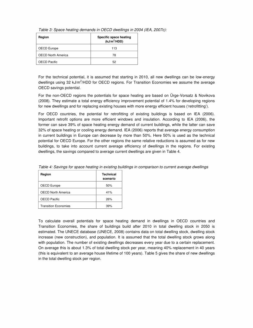
Table 3: Space heating demands in OECD dwellings in 2004 (IEA, 2007c):

Region Specific space heating

(kJ/m2/HDD)

OECD Europe 113

OECD North America 78

OECD Pacific 52

For the technical potential, it is assumed that starting in 2010, all new dwellings can be low-energy dwellings using 32 kJ/m2/HDD for OECD regions. For Transition Economies we assume the average OECD savings potential.

For the non-OECD regions the potentials for space heating are based on Ürge-Vorsatz & Novikova (2008). They estimate a total energy efficiency improvement potential of 1.4% for developing regions for new dwellings and for replacing existing houses with more energy efficient houses (‘retrofitting’).

For OECD countries, the potential for retrofitting of existing buildings is based on IEA (2006). Important retrofit options are more efficient windows and insulation. According to IEA (2006), the former can save 39% of space heating energy demand of current buildings, while the latter can save 32% of space heating or cooling energy demand. IEA (2006) reports that average energy consumption in current buildings in Europe can decrease by more than 50%. Here 50% is used as the technical potential for OECD Europe. For the other regions the same relative reductions is assumed as for new buildings, to take into account current average efficiency of dwellings in the regions. For existing dwellings, the savings compared to average current dwellings are given in Table 4.

Table 4: Savings for space heating in existing buildings in comparison to current average dwellings

Region Technical

scenario

OECD Europe 50%

OECD North America 41%

OECD Pacific 26%

Transition Economies 39%

To calculate overall potentials for space heating demand in dwellings in OECD countries and Transition Economies, the share of buildings build after 2010 in total dwelling stock in 2050 is estimated. The UNECE database (UNECE, 2008) contains data on total dwelling stock, dwelling stock increase (new construction), and population. It is assumed that the total dwelling stock grows along with population. The number of existing dwellings decreases every year due to a certain replacement. On average this is about 1.3% of total dwelling stock per year, meaning 40% replacement in 40 years (this is equivalent to an average house lifetime of 100 years). Table 5 gives the share of new dwellings in the total dwelling stock per region.

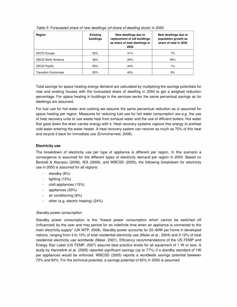
Table 5: Forecasted share of new dwellings (of share of dwelling stock) in 2050

Region Existing

buildings

New dwellings due to

replacement of old buildings

as share of total dwellings in

2050

New dwellings due to

population growth as

share of total in 2050

OECD Europe 52% 41% 7%

OECD North America 36% 29% 35%

OECD Pacific 55% 44% 1%

Transition Economies 55% 45% 0%

Total savings for space heating energy demand are calculated by multiplying the savings potentials for new and existing houses with the forecasted share of dwelling in 2050 to get a weighed reduction percentage. For space heating in buildings in the services sector the same percentual savings as for dwellings are assumed.

For fuel use for hot water and cooking we assume the same percentual reduction as is assumed for space heating per region. Measures for reducing fuel use for hot water consumption are e.g. the use of heat recovery units to use waste heat from exhaust water and the use of efficient boilers. Hot water that goes down the drain carries energy with it. Heat recovery systems capture this energy to preheat cold water entering the water heater. A heat recovery system can recover as much as 70% of this heat and recycle it back for immediate use (Enviroharvest, 2008).

Electricity use

The breakdown of electricity use per type of appliance is different per region. In this scenario a convergence is assumed for the different types of electricity demand per region in 2050. Based on Bertoldi & Atanasiu (2006), IEA (2006), and WBCSD (2005), the following breakdown for electricity use in 2050 is assumed for all regions:

- standby (8%)

- lighting (15%)

- cold appliances (15%)

- appliances (30%)

- air conditioning (8%)

- other (e.g. electric heating) (24%)

Standby power consumption

Standby power consumption is the "lowest power consumption which cannot be switched off (influenced) by the user and may persist for an indefinite time when an appliance is connected to the main electricity supply" (UK MTP, 2008). Standby power accounts for 20–90W per home in developed nations, ranging from 4 to 10% of total residential electricity use (Meier et al., 2004) and 3-12% of total residential electricity use worldwide (Meier, 2001). Efficiency recommendations of the US FEMP and Energy Star Label (US FEMP, 2007) assume best practice levels for all equipment of 1 W or less. A study by Harmelink et al. (2005) reported significant savings (up to 77%) if a standby standard of 1W per appliances would be enforced. WBCSD (2005) reports a worldwide savings potential between 72% and 82%. For the technical potential, a savings potential of 82% in 2050 is assumed.

Lighting

In indicator for the efficiency of lighting is the luminous efficacy (mW/lm) of average lamps used in a region. The luminous efficacy is a ratio of the visible light energy emitted (the luminous flux) to the total power input to the lamp. It is measured in lumens per watt (lm/W). The maximum efficacy possible is 240 lm/W for white light. The current best practice is 75 lm/W for fluorescent lights (future fluorescent lights 100 lm/W) and 115 lm/W for white LEDs (future LEDs 150 lm/W) (LEDS Magazine, 20078). The luminous efficacy of incandescent lamps is 10-17 lm/W. For the technical potential in 2050 we assume that the average luminous efficacy can be increased to 100 lm/W in all regions.

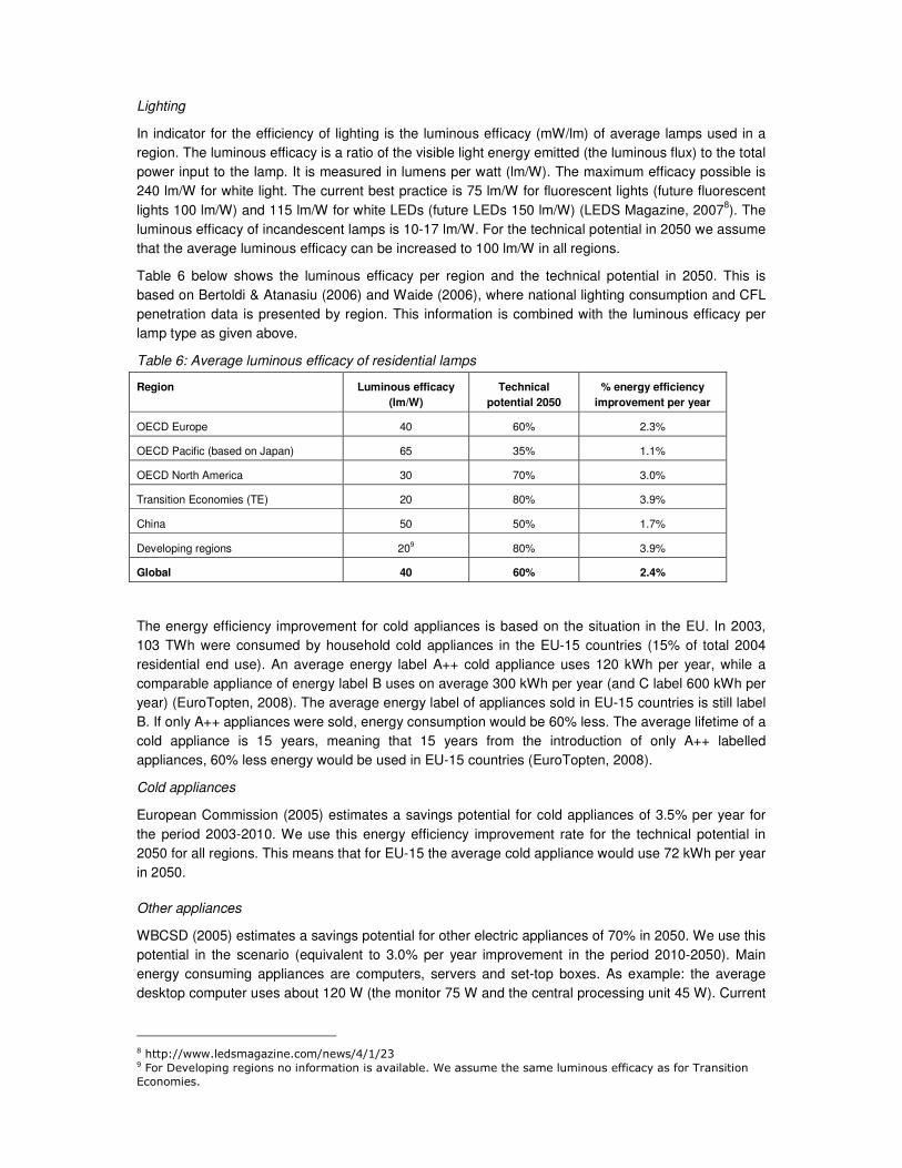
Table 6 below shows the luminous efficacy per region and the technical potential in 2050. This is based on Bertoldi & Atanasiu (2006) and Waide (2006), where national lighting consumption and CFL penetration data is presented by region. This information is combined with the luminous efficacy per lamp type as given above.

Table 6: Average luminous efficacy of residential lamps

Region Luminous efficacy

(lm/W)

Technical

potential 2050

% energy efficiency

improvement per year

OECD Europe 40 60% 2.3%

OECD Pacific (based on Japan) 65 35% 1.1%

OECD North America 30 70% 3.0%

Transition Economies (TE) 20 80% 3.9%

China 50 50% 1.7%

Developing regions 209 80% 3.9%

Global 40 60% 2.4%

The energy efficiency improvement for cold appliances is based on the situation in the EU. In 2003, 103 TWh were consumed by household cold appliances in the EU-15 countries (15% of total 2004 residential end use). An average energy label A++ cold appliance uses 120 kWh per year, while a comparable appliance of energy label B uses on average 300 kWh per year (and C label 600 kWh per year) (EuroTopten, 2008). The average energy label of appliances sold in EU-15 countries is still label B. If only A++ appliances were sold, energy consumption would be 60% less. The average lifetime of a cold appliance is 15 years, meaning that 15 years from the introduction of only A++ labelled appliances, 60% less energy would be used in EU-15 countries (EuroTopten, 2008).

Cold appliances

European Commission (2005) estimates a savings potential for cold appliances of 3.5% per year for the period 2003-2010. We use this energy efficiency improvement rate for the technical potential in 2050 for all regions. This means that for EU-15 the average cold appliance would use 72 kWh per year in 2050.

Other appliances

WBCSD (2005) estimates a savings potential for other electric appliances of 70% in 2050. We use this potential in the scenario (equivalent to 3.0% per year improvement in the period 2010-2050). Main energy consuming appliances are computers, servers and set-top boxes. As example: the average desktop computer uses about 120 W (the monitor 75 W and the central processing unit 45 W). Current

8 http://www.ledsmagazine.com/news/4/1/23 9 For Developing regions no information is available. We assume the same luminous efficacy as for Transition

Economies.

best practice monitors (Best of Europe, 2008) use only 18W (15 inch), which is 76% less than average.

Air conditioning

For air conditioning we assume a savings potential of 70% in 2050, similar to the potential reported in WBCSD (2005). The potential takes into account that a certain share of conventional air conditions is replaced by solar cooling and geothermal cooling and that the remaining units use refrigerant Ikon B. Tests with the refrigerant Ikon B show possible energy consumption reductions of 20-25% compared to regularly used refrigerants (US DOE EERE, 2008). Solar cooling is the use of solar thermal energy or solar electricity to power a cooling appliance. To drive the pumps only 0.05 kW of electricity is needed (instead of 0.35 kW for regular air conditioning) (Austrian Energy Agency, 2006), this calculates to a savings potential of 85%. Besides efficient air conditioning equipment, it is as important to reduce the need for air conditioning. Important ways to reduce cooling demand are: use insulation to prevent heat from entering the building, reduce the amount of inefficient appliances present in the house (such as incandescent lamps, old refrigerators, etc.) that give off unusable heat, use cool exterior finishes (such as cool roof technology (US EPA, 2007), or light-coloured paint on the walls) to reduce the peak cooling demand (as much as 10-15% according to ACEEE (2007)), improve windows and use vegetation to reduce the amount of heat that comes into the house, and use ventilation instead of air conditioning units.

2.2 Marginal costs of energy-efficiency measures

Costs for energy efficiency improvement are based on a selection of important measures for energy efficiency improvement. These measures are based on available literature sources that give estimates for costs and benefits of energy savings options. The options with the highest saving potential per sector are included. This results in 30 measures, which apply to 80% of the energy demand. For 20% of the energy demand (mainly in agriculture and some industrial sub sectors) no measures are included, due to lack of data. The measures have a savings potential of 40% of the energy demand they apply to.

Because energy prices and savings are different in different world regions we base the calculations on two world regions; OECD Europe and China. The reason for selecting OECD Europe is because many literature sources were available regarding costs and benefits of energy efficiency measures. China is selected because in the reference scenario it is the largest energy using region in 2050, consuming 21% of global energy demand.

The costs for energy efficiency measures are expressed as direct costs and refer to additional costs needed to implement a technological measure. Indirect cost savings from e.g. reduced environmental damage are not taken into account. We do not look at the rebound effect in this study (see e.g. Sorrel et al. (2004)).

Specific costs of a measure are calculated by summing annualised investment costs, operation and maintenance costs and savings per GJ energy saved. The specific costs can be negative if the benefits associated with the measure are sufficiently large. The costs calculated this way are life-cycle costs and represent total costs, taking into account the technical life span of the equipment.

The prices used are market prices. Taxes and levies are not included (e.g. value added tax or excise duties on fuel). In this study a discount rate of 6% is used.

The specific net costs for each measure (€/GJ) are determined as follows: Es = Cs - Ps

Where Es = specific net costs of measure (€/GJ)

Cs = specific costs of measure (€/GJ)

Ps = specific benefit of measure (€/GJ)

The specific costs Cs is calculated by dividing the annual costs of the option by the annual energy

savings: Cs = (α * Cinv + CO&M)/R

Where Cs = specific costs of measure (€/GJ)

Cinv = (additional) up front investment costs (€)

CO&M = yearly operation and maintenance costs (€/year)

α = annuity factor: r/(1-(1+r)-n)

r = discount rate (in %/year)

n = lifetime of the investment (i.e. depreciation period in years)

R = annual energy savings (GJ/year)

The specific benefits of a measure Ps are calculated by dividing the annual benefits by the annual energy savings: Ps = P / R

Where Ps = specific benefits of measure (€o/GJ)

P = annual benefits from energy savings (€o/year)

R = annual energy savings (GJ/year)

The costs in this study are expressed in Euros (€) with a 2005 price level. Conversion rates are based on IMF (2008).

Prices are based on purchasing power parities (PPP). PPP compare costs in different currencies of a fixed basket of traded and non-traded goods and services and yield a widely-based measure of standard of living. Therefore they have a more direct link with energy use than prices based on market exchange rates. For converting from the Chinese currency Yuan (CNY) to Euro (€) we use the conversion rate of 1 CNY2005 = 0.4 €2005. This is based on a PPP correction rate of 0.25 in 2005 (note: US$ = 1) (Nation Master, 2008) and the exchange rate of 1 CNY2005 = 0.12 US$2005 (X-rates, 2008).

Fuel prices for OECD Europe are based on Eurostat (2007)10. The price for natural gas is in €2005/GJ final energy, 12 for households, 9 for services and 7 for industries. For transport the prices are 13 €/GJ for diesel oil and gasoline and 21 for kerosene. The electricity price is 42 €/GJ for households, 35 for services and 28 for industries. The price for coal in industries is 2 €/GJ.

For China energy prices are based on Pachauri and Jiang (2008) and IEA Energy Prices and taxes 2007. The energy prices in China and OECD Europe are very similar as expressed in PPP. There are two main differences. In China currently a lot of biomass and coal is used for heating in households at low prices. Costs of biomass use in households amounts to 2 €/GJ and of coal use 5 €/GJ. Furthermore, electricity prices in China are significantly lower than in OECD Europe (30 €/GJ for households, 17 for services and 14 for industries). According to Lam (2001) electricity prices in China are highly subsidised and well below costs for generation and transmission. This is because capital costs of state-owned power plants are often not reflected in electricity prices. It seems likely that with the growing economy in China the use of wood stoves will take a lower share in energy demand for

10 Prices are for the second quarter 2007 for EU27 excluding taxes in €2005 prices (prices for natural gas GCV are

converted to NCV by factor 0.9).

heating in the future and energy prices in households will become more similar to current prices in OECD Europe. We therefore use 12 €/GJ for fuel costs for heating in households (equal to current natural gas price in China). For the electricity prices we just assume current values in China, but it may be that measures will become more profitable if electricity prices increase over time and subsidies decrease.

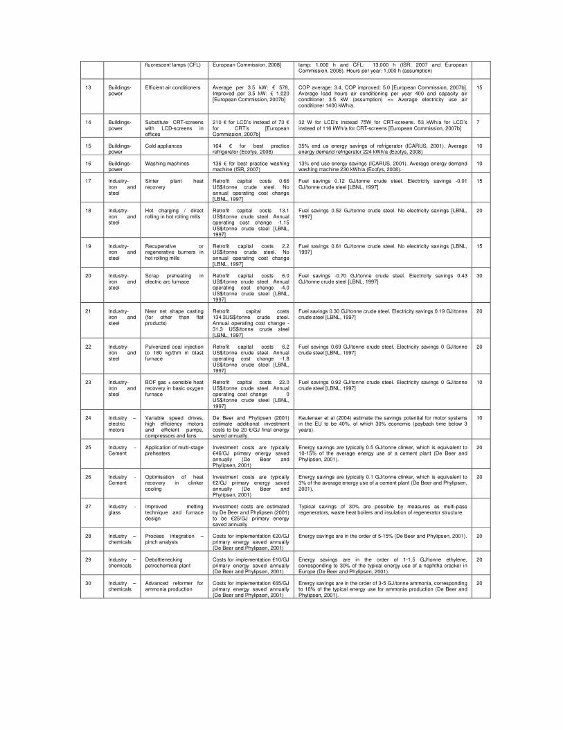
Table 7 shows the measures for which costs are calculated and the key assumptions regarding investments costs and energy savings.

Table 7: Included measures and key assumptions

Nr. Sector Measure Investment costs (additional) Energy savings Life-time (yr)

1 Transport – passenger cars

Hybrid passenger cars 2000-2500 USD for petrol hybrid, 5000-5500 USD for hybrid diesel [Frost and Sullivan, 2008 and TNO et al., 2006] As average we take 3000 €

Average mileage 12,500 km per year OECD Europe, 10,000 km per year China (IEA/SMP, 2004). Default car 13 km /litre g.e. for OECD Europe and 9 km /litre g.e. for China (IEA/SMP, 2004). Hybrid car 20 km /litre g.e. (Toyota, 2008).

10

2 Transport – passenger cars

Weight reduction of passenger cars

2185 € (diesel) – 1619 € (petrol) [TNO et al., 2006 and JRC, 2008] As average we take 1800 €

18% savings (TNO et al., 2006 and JRC, 2008). Average mileage 12,500 km per year OECD Europe, 10,000 km per year China (IEA/SMP, 2004). Default car 13 km /litre g.e. for OECD Europe and 9 km /litre g.e. for China (IEA/SMP, 2004).

10

3 Transport-buses

Hybrid buses Additional investment costs: 150,000 – 200,000 US$ (EESI 2006). As average we take 175,000US$. Additional maintenance costs: 0.02 US$/mile (EESI 2006)

Travel per vehicle: 60,000 km per year OECD Europe, 40,000 km per year China. Improve of efficiency: 25 – 45% � as average 35% (IEA SMP, 2004). Default bus 3.03 km/l OECD Europe, 3.57 km/l China (IEA SMP, 2004)

10

4 Transport-trucks

Improved aerodynamics, Tyre inflation control (TPMS), Use of wide-based tires, Reduce engine idling, Driver training

8000 € (US EPA, 2008) 13% savings (US EPA, 2008). Average mileage 60,000 km per year OECD Europe, 50,000 km per year China (IEA/SMP, 2004). Default truck 1.6 MJ/t.km for OECD Europe and 2.0 MJ/t.km for China (IEA/SMP, 2004). Average truck load 8 tonnes for OECD Europe and 6 tonnes for China (IEA/SMP, 2004).

10

5 Transport - aviation

Improved aerodynamics, Advanced engines, Improved Air Traffic Management (ATM), Further operational measures

1.4 mio € (IPCC, 2007 and IPTS, 2008)

30% (IPCC (2007) and IPTS (2008)). 2.6 MJ/p-km in China and OECD Europe (IEA/SMP, 2004). Number of passenger per aircraft 300 (assumption). Mileage 400,000 km per year (assumption).

10

6 Buildings-heat

Passive houses – new buildings

95 €/m² based on 7-12% higher price than new buildings (standard buildings costs of 1,000€ per m²) [Passivehaus Institut, Darmstadt]

Energy demand passive house: 54 MJ/m²a space heating demand (Passivehaus Institut, Darmstadt). The energy demand for average new houses equals 270 MJ/m²a in EU27 (Harmelink, 2008). The relative improvement potential in China is assumed to be the same as for EU27 (63% for new buildings). Average energy demand in households for heating amounted to around 200 MJ/m2aGJ per household (Zhang, 2004) For the average dwelling size in China we assume 70 m2.

30

7 Buildings-heat

Roof insulation - existing buildings

30 €/m2 (Boermans and Petersdorff, 2007)

Existing roofs of buildings built before 1975 in moderate climate EU-27: 1.5 W/m²K. After insulation in moderate climate: 0.17 W/m²K. Heat degree days 2900 Kd/a in OECD Europe (Boermans and Petersdorff (2007) for EU27) and 2750 Kd/a average in China (Zhang, 2004). Average roof area 43 m2 for OECD Europe (0.5*average area dwelling; 85 m2 in EU27 (Ecofys, 2008)) and 35 for China (based on average dwelling area of 70 m2)

30

8 Buildings-heat

Wall insulation - existing buildings


Existing walls of buildings built before 1975 in moderate climate EU27: 1.5 W/m²K. After insulation in moderate climate: 0.22 W/m²K (Boermans and Petersdorff, 2007). Heat degree days 2900 Kd/a in OECD Europe (Boermans and Petersdorff (2007) for EU27) and 2750 Kd/a average in China (Zhang, 2004). Average wall surface is 60 m2 for OECD Europe (0.7*average area dwelling; is 85 m2 in EU27 (Ecofys, 2008)) and 49 m2 for China (based on average dwelling area of 70 m2)

30

9 Buildings-heat

Floor insulation - existing buildings


Existing floors of buildings built before 1975 in moderate climate EU27: 1.2 W/m²K. After insulation in moderate climate: 0.28 W/m²K (Boermans and Petersdorff, 2007). Heat degree days 2900 Kd/a in OECD Europe (Boermans and Petersdorff (2007) for EU27) and 2750 Kd/a average in China (Zhang, 2004). Average floor area is 43 m2 for OECD Europe (0.5*average area dwelling; is 85 m2 in EU27 (Ecofys, 2008)) and 35 m2 for China (based on average dwelling area of 70 m2)

30

10 Buildings-heat

Window insulation - existing buildings

100 €/m2 (Ecofys, 2008) Existing windows of buildings built before 1975 in moderate climate EU27: 3.5 W/m²K. After insulation in moderate climate: 1.2 W/m²K (Boermans and Petersdorff, 2007). Heat degree days 2900 Kd/a in OECD Europe (Boermans and Petersdorff (2007) for EU27) and 2750 Kd/a average in China (Zhang, 2004). Average window area is 13 m2 for OECD Europe (0.15*average area dwelling; is 85 m2 in EU27 (Ecofys, 2008)) and 11 m2 for China (based on average dwelling area of 70 m2)

30

11 Buildings-heat

Water saving power heads

Additional investment costs taps per dwelling: 27.0 € (Bettgenhäuser et al., 2008)

12.5% of energy use shower (Bettgenhäuser et al., 2008). Fraction of hot tap water through shower taps of total hot tap water: 50% (Ecofys, 2008). Energy use for hot tap water: 4.5 GJ/dwelling EU27 (Ecofys, 2008)

10

12 Buildings-power

Substitute incandescent lamps with compact

0.3 €/ klm for incandescent and 1.0 €/ klm CFL [ISR, 2007 and

Luminous efficacy range: 73 lm/W for CFL and 16 lm/W for incandescent (ISR, 2007 and European Commission, 2008). Lifespan incandescent

10

fluorescent lamps (CFL) European Commission, 2008]

lamp: 1,000 h and CFL: 13,000 h (ISR, 2007 and European Commission, 2008). Hours per year: 1,000 h (assumption)

13 Buildings-power

Efficient air conditioners Average per 3.5 kW: € 578, Improved per 3.5 kW: € 1,020 [European Commission, 2007b]

COP average: 3.4, COP improved: 5.0 [European Commission, 2007b]. Average load hours air conditioning per year 400 and capacity air conditioner 3.5 kW (assumption) => Average electricity use air conditioner 1400 kWh/a.

15

14 Buildings-power

Substitute CRT-screens with LCD-screens in offices

210 € for LCD’s instead of 73 € for CRT’s [European Commission, 2007b]

32 W for LCD’s instead 75W for CRT-screens. 53 kWh/a for LCD’s instead of 116 kWh/a for CRT-screens [European Commission, 2007b]

7

15 Buildings-power

Cold appliances 164 € for best practice refrigerator (Ecofys, 2008)

35% end us energy savings of refrigerator (ICARUS, 2001). Average energy demand refrigerator 224 kWh/a (Ecofys, 2008)

10

16 Buildings-power

Washing machines 136 € for best practice washing machine (ISR, 2007)

13% end use energy savings (ICARUS, 2001). Average energy demand washing machine 230 kWh/a (Ecofys, 2008).

10

17 Industry-iron and steel

Sinter plant heat recovery

Retrofit capital costs 0.66 US$/tonne crude steel. No annual operating cost change [LBNL, 1997]

Fuel savings 0.12 GJ/tonne crude steel. Electricity savings -0.01 GJ/tonne crude steel [LBNL, 1997]

15


Hot charging / direct rolling in hot rolling mills

Retrofit capital costs 13.1 US$/tonne crude steel. Annual operating cost change -1.15 US$/tonne crude steel [LBNL, 1997]

Fuel savings 0.52 GJ/tonne crude steel. No electricity savings [LBNL, 1997]

20


Recuperative or regenerative burners in hot rolling mills

Retrofit capital costs 2.2 US$/tonne crude steel. No annual operating cost change [LBNL, 1997]

Fuel savings 0.61 GJ/tonne crude steel. No electricity savings [LBNL, 1997]

15


Scrap preheating in electric arc furnace


Fuel savings -0.70 GJ/tonne crude steel. Electricity savings 0.43 GJ/tonne crude steel [LBNL, 1997]

30


Near net shape casting (for other than flat products)

Retrofit capital costs 134.3US$/tonne crude steel. Annual operating cost change -31.3 US$/tonne crude steel [LBNL, 1997]

Fuel savings 0.30 GJ/tonne crude steel. Electricity savings 0.19 GJ/tonne crude steel [LBNL, 1997]

20


Pulverized coal injection to 180 kg/thm in blast furnace


Fuel savings 0.69 GJ/tonne crude steel. Electricity savings 0 GJ/tonne crude steel [LBNL, 1997]

20


BOF gas + sensible heat recovery in basic oxygen furnace

Retrofit capital costs 22.0 US$/tonne crude steel. Annual operating cost change 0 US$/tonne crude steel [LBNL, 1997]

Fuel savings 0.92 GJ/tonne crude steel. Electricity savings 0 GJ/tonne crude steel [LBNL, 1997]

10

24 Industry – electric motors

Variable speed drives, high efficiency motors and efficient pumps, compressors and fans

De Beer and Phylipsen (2001) estimate additional investment costs to be 20 €/GJ final energy saved annually.

Keulenaer et al (2004) estimate the savings potential for motor systems in the EU to be 40%, of which 30% economic (payback time below 3 years).

10

25 Industry - Cement

Application of multi-stage preheaters

Investment costs are typically €46/GJ primary energy saved annually (De Beer and Phylipsen, 2001)

Energy savings are typically 0.5 GJ/tonne clinker, which is equivalent to 10-15% of the average energy use of a cement plant (De Beer and Phylipsen, 2001).

20

26 Industry - Cement

Optimisation of heat recovery in clinker cooling

Investment costs are typically €2/GJ primary energy saved annually (De Beer and Phylipsen, 2001)

Energy savings are typically 0.1 GJ/tonne clinker, which is equivalent to 3% of the average energy use of a cement plant (De Beer and Phylipsen, 2001).

20

27 Industry - glass

Improved melting technique and furnace design

Investment costs are estimated by De Beer and Phylipsen (2001) to be €25/GJ primary energy saved annually

Typical savings of 30% are possible by measures as multi-pass regenerators, waste heat boilers and insulation of regenerator structure.

28 Industry –chemicals

Process integration – pinch analysis

Costs for implementation €20/GJ primary energy saved annually (De Beer and Phylipsen, 2001)

Energy savings are in the order of 5-15% (De Beer and Phylipsen, 2001). 20


Debottlenecking petrochemical plant


Energy savings are in the order of 1-1.5 GJ/tonne ethylene, corresponding to 30% of the typical energy use of a naphtha cracker in Europe (De Beer and Phylipsen, 2001).

20


Advanced reformer for ammonia production


Energy savings are in the order of 3-5 GJ/tonne ammonia, corresponding to 10% of the typical energy use for ammonia production (De Beer and Phylipsen, 2001).

20

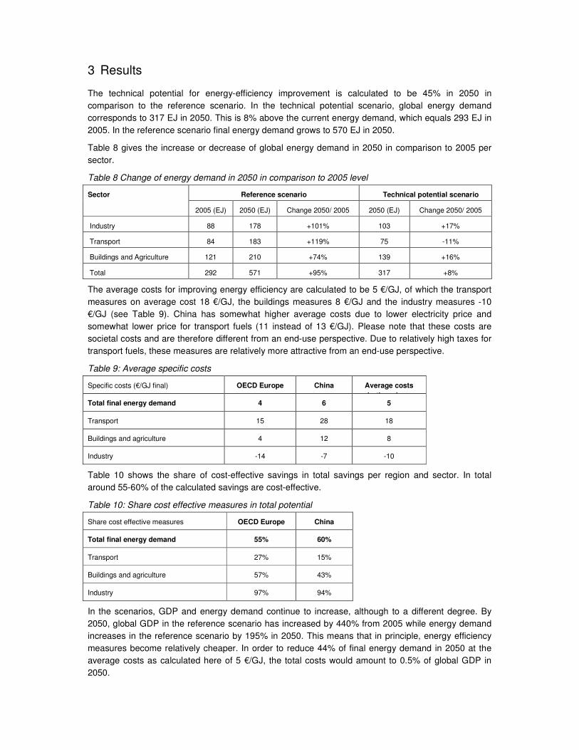
3 Results

The technical potential for energy-efficiency improvement is calculated to be 45% in 2050 in comparison to the reference scenario. In the technical potential scenario, global energy demand corresponds to 317 EJ in 2050. This is 8% above the current energy demand, which equals 293 EJ in 2005. In the reference scenario final energy demand grows to 570 EJ in 2050.

Table 8 gives the increase or decrease of global energy demand in 2050 in comparison to 2005 per sector.

Table 8 Change of energy demand in 2050 in comparison to 2005 level

Reference scenario Technical potential scenario Sector

2005 (EJ) 2050 (EJ) Change 2050/ 2005 2050 (EJ) Change 2050/ 2005

Industry 88 178 +101% 103 +17%

Transport 84 183 +119% 75 -11%

Buildings and Agriculture 121 210 +74% 139 +16%

Total 292 571 +95% 317 +8%

The average costs for improving energy efficiency are calculated to be 5 €/GJ, of which the transport measures on average cost 18 €/GJ, the buildings measures 8 €/GJ and the industry measures -10 €/GJ (see Table 9). China has somewhat higher average costs due to lower electricity price and somewhat lower price for transport fuels (11 instead of 13 €/GJ). Please note that these costs are societal costs and are therefore different from an end-use perspective. Due to relatively high taxes for transport fuels, these measures are relatively more attractive from an end-use perspective.

Table 9: Average specific costs

Specific costs (€/GJ final) OECD Europe China Average costs

both regions Total final energy demand 4 6 5

Transport 15 28 18

Buildings and agriculture 4 12 8

Industry -14 -7 -10

Table 10 shows the share of cost-effective savings in total savings per region and sector. In total around 55-60% of the calculated savings are cost-effective.

Table 10: Share cost effective measures in total potential

Share cost effective measures OECD Europe China

Total final energy demand 55% 60%

Transport 27% 15%

Buildings and agriculture 57% 43%

Industry 97% 94%

In the scenarios, GDP and energy demand continue to increase, although to a different degree. By 2050, global GDP in the reference scenario has increased by 440% from 2005 while energy demand increases in the reference scenario by 195% in 2050. This means that in principle, energy efficiency measures become relatively cheaper. In order to reduce 44% of final energy demand in 2050 at the average costs as calculated here of 5 €/GJ, the total costs would amount to 0.5% of global GDP in 2050.

Long term energy efficiency improvement requires continuous innovation and therefore besides current best practices, new measures will need to be implemented in the period up to 2050 to achieve the technical potentials. The costs needed to implement emerging innovative technologies are unknown, however, and may be more expensive than current best practice technologies as calculated here. On the other hand, fuel prices are likely to increase in the future, which has a large impact on the profitability of energy efficiency measures. This is further discussed in section 4 Discussion of uncertainties. Also learning effects, which tend to decrease prices when a technology is more frequently used are not taken into account.

The cost estimate does not take peripheral benefits of improved energy efficiency into account such as reduced fossil fuel consumption (leading to reduced pollution, decreased fossil fuel dependence, health improvement). Investments in energy efficiency generally lead to avoided costs for new heat and power generation capacity. The International Energy Agency (IEA) has estimated that $700 billion invested in energy efficiency worldwide between now and 2030 would result in returns of more than $1.4 trillion in terms of avoided supply-side investment (SDI, 2006). Moreover, the costs resulting from the effects of climate change are not taken into account.

4 Discussion of uncertainties

The global potential for energy efficiency improvement from a demand side point of view is estimated to be 2.4% per year for the period 2010-2050. Taking into account, the autonomous energy efficiency improvement (assumed to be 1% per year) this leads to a potential of 1.5% per year in comparison to the reference scenario.

The uncertainty in this estimate is high and depends largely on the assumptions used. The study is meant to show the important role energy efficiency should play in reducing greenhouse gas emissions. The calculations are conservative and are based on technical measures, which are either already available or should become available in the next decades. There is an additional potential for reducing energy demand by behavioral or organizational changes. These can be modal shift in transport from car to rail or the use of more daylight instead of artificial light in buildings.

Also the costs estimates have a high uncertainty. They are e.g. sensitive to the discount rate used and to fuel price assumptions. If the discount rate is changed from 6% to 4%, the average costs for the energy efficiency measures decrease from 5 €/GJ to 3 €/GJ. If the discount rate is changed to 8% the average costs increase to 8 €/GJ.

The results are very sensitive to the energy price assumptions. If fuel prices increase by 50% the average costs decrease from 5 €/GJ to -1 €/GJ. If fuel prices decrease by 50% the average costs increase to 12 €/GJ. As a comparison, in the WEO 2006 oil prices increase by 9% in the period 2005-2030, coal prices decrease by 4% and natural gas price increases by 13%.

Based on these uncertainties we estimate the yearly costs are in the range of a -2% and 2% of GDP in 2050.

5 Conclusions

By implementing the technical measures for energy efficiency improvement, the expected growth of final energy demand can be limited to 8% (from 293 to 317 EJ) instead of 95% (from 293 to 570 EJ). If greenhouse gas intensity of energy demand (in kg CO2/ GJ) is the same, this means that greenhouse gas emissions resulting from energy use will be 45% lower in 2050 in comparison to the reference scenario. This makes energy-efficiency improvement a crucial part in any greenhouse gas abatement strategy.

Costs for implementing the energy efficiency measures are limited from a global perspective and are estimated to be in the range of -2% to 2% of global GDP in 2050. More than 50% of (the savings of) the measures are cost-effective. In these cases fuel savings compensate for (incremental) investment costs (depending on discount rate use and fuel price assumptions).

This study looks at energy-efficiency improvement from a demand side perspective. There is an additional potential for energy-efficiency improvement in the transformation sector. In 2005 the global average conversion efficiency equals 68% and is different per world region and ranges from 62% for China to 78% for Latin America. The low conversion efficiency for China is mainly a result of the large share of coal-fired power generation at low efficiency. The relatively high efficiency for Latin America is mainly a result of a high share of hydropower in power generation. In IEA statistics the conversion of electricity generated by hydropower to primary energy input is 100%.

Graus et al (2009) estimate that the global conversion efficiency can be improved from 68% in 2005 to 81% in 2050 mainly by increased energy-efficiency of power generation (e.g. 53% average efficiency for fossil-fired power generation in 2050 in comparison to 33% in 2005). With a conversion efficiency of 81%, primary energy supply in the technical potential scenario would then decrease by 10% from 432 EJ in 2005 to 391 EJ in 2050. Including the transformation sector, the total potential for energy-efficiency improvement would then be 55% in 2050, in comparison to business as usual development of energy supply.

Acknowledgement

This paper is based on scenarios developed for DLR, Greenpeace / EREC and UBA. The views expressed in this paper do not necessarily reflect their views. We would like to thank Ernst Worrell for reviewing an earlier draft of this paper.

References

� ACEEE (American Council for an Energy-Efficient Economy) (2007): Consumer Guide to Home Energy Savings - Cooling

Equipment. http://www.aceee.org/consumerguide/cooling.htm#reduce

� Akerman, J. (2005): Sustainable air transport–on track in 2050. Transportation Research Part D 10, pp. 111-125.

� Bertoldi, P. and B. Atanasiu. (2006): Electricity Consumption and Efficiency Trends in the Enlarged European Union –

Status Report 2006. Institute for Environment and Sustainability.

� Bettgenhäuser, K., T. Boermans, M. Anger and S. Lindner (2008). SERPEC-CC – Residential buildings and services

sector: description of approach. Draft version. Confidential. Ecofys.

� Blok, K. (2005): Improving energy-efficiency by five percent and more per year? Journal of Industrial Ecology. Volume 8,

Number 4. Massachusetts Institute of Technology and Yale University.

� Boermans, T. and C. Petersdorff (2007). U-values for better energy performance of buildings.

� De Beer, J. and D. Phylipsen (2001). Economic evaluation of Carbon Dioxide and Nitrous Oxide emission reduction in the

EU. Ecofys, Netherlands.

� DeCicco, J., F. An, and M. Ross (2001). Technology Options for Improving the Fuel Economy of U.S. Cars and Light

Trucks by 2010–2015. American Council for an Energy Efficient Economy, Washington, D.C

� Ecofys (2008). SERPEC-CC. Bottum-up report. Draft version. Confidential. Ecofys

� Ecofys and Utrecht University (2001). ICARUS-4: Sector Study for the Households.

� Enviroharvest (2008). Heat recovery. http://www.enviroharvest.ca/heat_recovery.htm

� European Commission (2005): Doing more with less - Green paper energy-efficiency. European Communities.

http://ec.europa.eu/energy/efficiency/index_en.htm

� European Commission (2008). Preparatory study on the environmental performance of residential room conditioning

appliances. Draft report of Task 7: Improvement Potential; Service Contract to DGTREN, March 2008. p.28.

� European Commission (EC), 2006. Reference document on best available techniques for large combustion plants.

� Frost and Sullivan (2008) http://www.automotive.frost.com.

� EuroTopten (2008): Best Products of Europe. Energy consumption and saving potentials.

http://www.topten.info/index.php?page=energy_consumption_and_saving_potentials

� Graus, W., C. Klessmann, C. Capone and E. Stricker (2009). Global potentials of energy-efficiency. Work package 4 of

“The role and potential of renewable energy and energy efficiency for global energy supply” by DLR / Ecofys / Wuppertal

Institute. Commissioned by Ministry of Environment, Germany.

� IEA (2006): Energy Technology Perspectives 2006 – Scenarios and Strategies to 2050. International Energy Agency,

Paris, 2006.

� IEA (2007a). Energy balances of OECD countries 1960-2005 and Energy balances of non-OECD countries 1971-2005.

International Energy Agency (IEA). Paris, France.

� IEA (2007b). World Energy Outlook 2007 edition. International Energy Agency (IEA). Paris, France.

� IEA (2007c). Energy use in the New Millennium – Trends in IEA Countries. OECD/International Energy Agency.

� IEA (2008): Energy Technology Perspectives 2008 – Scenarios and Strategies to 2050. International Energy Agency,

Paris, 2008.

� IEA/SMP (2004). IEA/SMP Model Documentation and Reference Case Projection. L. Fulton (IEA) and G. Eads (CRA) for

WBCSD’s Sustainable Mobility Project (SMP), July 2004.

� IMF (2008). World Economic Outlook, International Monetary Fund. http://www.imf.org/external/ns/cs.aspx?id=28

� IPCC (2007). Aviation and the global atmosphere, IPCC report: http://www.grida.no/climate/ipcc/aviation/088.htm

� ISR (2007). Residential Monitoring to Decrease Energy Use and Carbon Emissions in Europe. ISR-University of Coimbra,

Portugal, Dep. Electrical Engineering, February 2007.

� Joosen et al. (2002). Sectoral objectives of emission reduction. Assignment for European Commission. http://ec.europa.eu/environment/enveco/climate_change/pdf/top_down_analysis_xsum.pdf

� JRC (2008). Environmental Improvement Potential of Cars (IMPRO-Car), JRC Scientific and Technical report, eur 23038

En, April 2008, available at: http://www.jrc.es/publications/pub.cfm?id=1564

� Lam, P. (2001). Pricing of electricity in China. The Hong Kong Polytechnic University, Faculty of Business, Room M846,

Hung Hom, Hong Kong Received 22 October 2001 Energy 29 (2004) 287–300

� LBNL (1997). Energy-efficiency improvement and costs in iron and steel industry. Lawrence Berkeley National Laboratory

(LBNL). Berkeley, United States.

� Lensink, S.M and H. de Wilde. March 2007. Kostenefficientie van (technische) opties voor zuiniger vrachtverkeer. Energy

research Centre of The Netherlands (ECN). http://www.ecn.nl/docs/library/report/2007/e07003.pdf

� Nation Master (2008). http://www.nationmaster.com/graph/cur_ppp_con_fac_to_off_exc_rat_rat-factor-official-exchange-

rate-ratio

� Neelis, M. and M. Patel (2006). Long-term production, energy consumption and CO2 emission scenarios for the worldwide

iron and steel industry. Utrecht University.

� ODYSSEE (2005). Energy efficiency indicators database ENERDATA. France.

� Pachauri, S. and L. Jiang (2008). "The Household Energy Transition in India and China." IIASA Interim Report IR-08-009,

May 2008Phylipsen, G.J.M. (2000). International Comparisons & National Commitments, Analysing energy and technology

differences in the climate debate, PhD thesis, April 2000, Utrecht University. Utrecht, The Netherlands.

� REEEP (2008). Global energy efficiency status report. Ecofys, Netherlands.

� Sorrel, S., E. O’Malley, J. Schleich and S. Scott Eds. 2004. The Economics of Energy efficiency. Edward Elgar,

Cheltenham, UK.

� SRU (German Advisory Council on the Environment) (2005). Reducing CO2 emissions from cars. Section from the Special

Report Environment and Road Transport.

www.lowcvp.org.uk/assets/reports/Reducing_CO2_Emissions%20Aug%2005.pdf

� Technical Options for Improving the Fuel Economy of U.S. Cars and Light Trucks by 2010-2015.

http://www.aceee.org/pubs/t012.htm

� Sinton, J.E., J.I. Lewis, L.K. Price and E. Worrell (2002): China’s sustainable energy future scenarios and carbon

emissions analysis. Subreport 11: international trends in energy-efficiency technologies and policies. LBNL, Berkeley, US.

� Smokers, R., R. Vermeulen, R. van Mieghem, R. Gense, I. Skinner, M. Fergusson, E. MacKay, P. ten Brink, G. Fontaras,

and Z. Samaras (2006): Review and analysis of the reduction potential and costs of technological and other measures to

reduce CO2-emissions from passenger cars. TNO, IEEP and LAT on behalf of the European Commission

(DG-ENTR) http://www.lowcvp.org.uk/assets/reports/TNO%20IEEP%20LAT%20et%20al%20report_co2_reduction.pdf

� Simon, S., W. Krewitt, and T. Pregger (2008): Energy [R]evolution scenario 2008. Working Paper on specification of world

regions, population development and GDP development. DLR, Institute of Technical Thermodynamics Systems Analysis

and Technology Assessment. Stuttgart.

� Stern (2006). Stern Review, “Economics of Climate Change”, 2006. http://www.hm-

treasury.gov.uk/stern_review_final_report.htm

� TNO et al. (2006). Review and analysis of the reduction potential and costs of technological and other measures to reduce

CO2-emissions from passenger cars, TNO, IEEP, LAT, 2006.

� Toyota (2008). http://www.toyota.com.au/prius

� UK MTP (United Kingdom Market Transformation Programme) (2008). BNXS15: Standby power consumption – domestic

appliances. http://www.mtprog.com/ApprovedBriefingNotes/PDF/MTP_BNXS15_2008February11.pdf

� UNECE (United Nations Economic Commission for Europe) (2008). Human Settlement Database.

http://w3.unece.org/stat/HumanSettlements.asp

� Ürge-Vorsatz, D. and A. Novikova (2008). Potentials and costs of carbon dioxide mitigation in the world’s buildings. Energy

Policy 36, pp. 642-661.

� US DOE EERE (United States Department of Energy; Energy-efficiency and Renewable Energy) (2008): Inventions &

Innovation Project Fact Sheet. High Energy-efficiency Air Conditioning.

http://www1.eere.energy.gov/inventions/pdfs/nimitz.pdf

� US EPA (United States Environmental Protection Agency) (2007): Cool Roofs.

http://www.epa.gov/heatisld/strategies/coolroofs.html

� U.S. Environmental Protection Agency (EPA) (2008). under the SmartWay Transport Partnership.

http://www.epa.gov/smartway/

� US FEMP (United States Federal Energy Management Program) (2007). How to buy products with low standby power.

http://www1.eere.energy.gov/femp/procurement/eep_standby_power.html

� X-rates (2008). http://www.x-rates.com/d/USD/CNY/hist2005.html

� Waide, P. (2007). Presentation of Light’s Labour’s Lost: Policies for Energy-efficient Lighting. OECD/IEA, 2007.

� WBCSD (World Business Council on Sustainable Development) (2005). Pathways to 2050 – Energy and Climate Change.

� Worrell (1994). Potentials for Improved Use of Industrial Energy and Materials, Ph.D. thesis, Utrecht University

� Worrell, E., L. Price, M. Neelis, C. Galitsky and Zhou Nan (2008). World Best Practice Energy Intensity Values for Selected

Industrial Sectors. Lawrence Berkeley National Laboratory (LBNL). Berkeley, United States.

� Zhang, Q. (2004). Residential energy consumption in China and its comparison with Japan, Canada, and USA . Tsukuba

College of Technology. Energy and Buildings. Volume 36, Issue 12, December 2004, Pages 1217-1225. Energy and

Environment of Residential Buildings in China.

ecofys netherlands bv - aaee

Documents