ECIV 720 A Advanced Structural

Mechanics and Analysis

Lecture 12: Isoparametric CST

Area CoordinatesShape FunctionsStrain-Displacement MatrixRayleigh-Ritz FormulationGalerkin Formulation

FEM Solution: Area Triangulation

Area is Discretized into Triangular Shapes

FEM Solution: Area Triangulation

One Source of Approximation

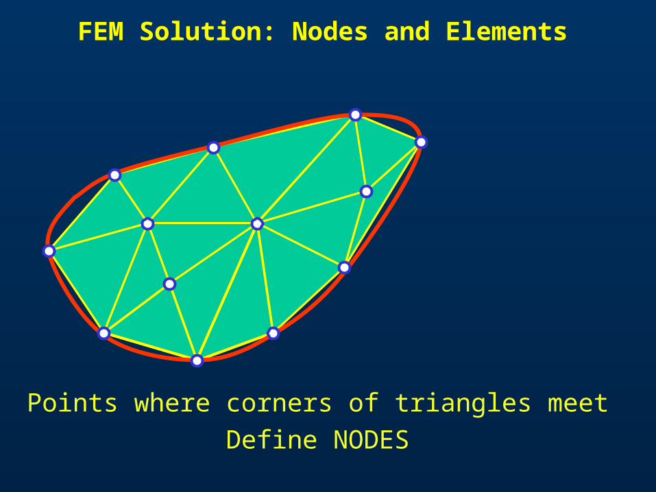
FEM Solution: Nodes and Elements

Points where corners of triangles meet

Define NODES

Non-Acceptable Triangulation

…

Nodes should be defined on corners of ALL adjacent triangles

FEM Solution: Nodes and Elements

Each node translates in X and Y

ui

vi

X

Y

FEM Solution: Objective

• Use Finite Elements to Compute Approximate Solution At Nodes

1 (x1,y1)2 (x2,y2)

3 (x3,y3)

q6

q5

q4

q3

q1

q2

vu

• Interpolate u and v at any point from Nodal values q1,q2,…q6

Intrinsic Coordinate System3 (x3,y3)

2 (x2,y2)

1 (x1,y1)

3 (0,0) 1 (1,0)

2 (0,1)

Map ElementDefine Transformation

Parent

Area Coordinates

A1

A

AL 1

1

A

AL 2

2

A

AL 3

3

1

2

3P

Area Coordinates

X

Y Location of P can be defined uniquely

Area Coordinates and Shape Functions

1L 2L 13L3 (x3,y3)

2 (x2,y2)1 (x1,y1)

Area Coordinates are linear functions of and

Are equal to 1 at nodes they correspond to

Are equal to 0 at all other nodes

3 (0,0) 1 (1,0)

2 (0,1)

Natural Choice for Shape Functions

Shape Functions

11 LN

22 LN

133 LN

X

Y

10

10

1 (x1,y1)2 (x2,y2)

3 (x3,y3)

Geometry from Nodal Values

332211 xNxNxNx

332221 yNyNyNy

11 LN

22 LN

133 LN

32313

33231

xxx

xxxxxx

32313

33231

yyy

yyyyyy

Intrinsic Coordinate System

32313 xxxx

Map ElementTransformation

3 (0,0) 1 (1,0)

2 (0,1)

Parent

3 (x3,y3)

2 (x2,y2)

1 (x1,y1)

32313 yyyy

Displacement Field from Nodal Values

533211 qNqNqNu

634221 qNqNqNv

12

3q6

q5

q4

q3

q2

q1

vu

Nqu

6

5

4

3

2

1

321

321

000

000

q

q

q

q

q

q

NNN

NNN

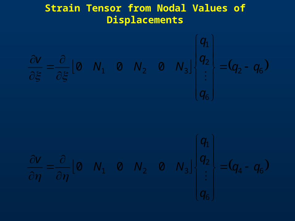
Strain Tensor from Nodal Values of Displacements

x

v

y

uy

vx

u

ε

y

v

x

v

x

u

y

u

Strain Tensor Need Derivatives

533211 qNqNqNu

634221 qNqNqNv

u and v functions of and

Jacobian of Transformation

y

y

ux

x

uu

y

y

ux

x

uu

y

y

vx

x

vv

y

y

vx

x

vv

y

ux

u

yx

yx

u

u

y

vx

v

yx

yx

v

v

J

J

Jacobian of Transformation

Jacobian of Transformation – Physical Significance

yx

yx

J

32313 xxxx 32313 yyyy

13xx

23x

x

13y

y

23y

y

2323

1313

yx

yxJ

Jacobian of Transformation – Physical Significance

3 (x3,y3)

2 (x2,y2)

1 (x1,y1)

r1 r2

jir 31311 yyxx

jir 32322 yyxx

k

kji

rr2323

1313

2323

131321

0

0yx

yx

yx

yx

Jacobian of Transformation – Physical Significance

3 (x3,y3)

2 (x2,y2)

1 (x1,y1)

r1 r2

krr2323

131321 yx

yx

k

elemA2det J

elemA2

2323

1313

yx

yxJ

Compare to Jacobian

Jacobian of Transformation

y

ux

u

u

u

J

1323

1323

1323

13231

2

1

det

1xx

yy

Axx

yy

elemJJ

u

u

y

ux

u

1JSolve

y

vx

v

v

v

J

v

v

y

vx

v

1JSolve

Strain Tensor from Nodal Values of Displacements

51

6

2

1

321 000 qq

q

q

q

NNNu

53

6

2

1

321 000 qq

q

q

q

NNNu

1N 2N 13N

Strain Tensor from Nodal Values of Displacements

62

6

2

1

321 000 qq

q

q

q

NNNv

64

6

2

1

321 000 qq

q

q

q

NNNv

Strain Tensor from Nodal Values of Displacements

6

2

1

122131132332

211332

123123

000

000

2

10

0

q

q

q

yxyxyx

xxx

yyy

Av

u

xy

y

x

elem ε

= B q

B q

Looks Familiar?

Strain-Displacement Matrix

6

2

1

122131132332

211332

123123

000

000

2

1

q

q

q

yxyxyx

xxx

yyy

Aelemxy

y

x

ε

Is constant within each element - CST

1 (x1,y1) 2 (x2,y2)

3 (x3,y3)

jiij yyy jiij xxx

Stresses

xy

y

x

xy

y

xE

2

100

01

01

1 2

Dεσ = B q

DBqσ

Element Stiffness Matrix ke

eV

Te dVU σDε

2

1

= B q= D B qe

e

A

TTe

el

TTe

e

dAt

tdA

U

e

qDBBq

qDBBq

2

1

2

1

ke

1 (x1,y1) 2 (x2,y2)

3 (x3,y3)

tdAdV

x

y

z

P

Formulation of Stiffness EquationsT (force/area)

Tt (force/length)

P

Assume

Plane

Stress

x

y

t

Total Potential Approach

i

iTiS

T

V

T

V

T dSdVdV PuTufuεσ2

1

P

Tt (force/length)

Total Potential

Total Potential Approach

i

iTiS

T

V

T

V

T dSdVdV PuTufuεσ2

1

P

Tt (force/length)

ii

Ti

el

T

eA

T

eA

T

ee

e

tdltdA

tdA

PuTufu

Dεε2

1

Total Potential Approach

ii

Ti

el

T

eA

T

eA

T

e

e

e

tdl

tdA

tdA

Pu

Tu

fu

Dεε2

1

eeTe

e

A

TTe

el

TTe

e

dAt

tdA

U

e

qkq

qDBBq

qDBBq

2

1

2

1

2

1

Total Potential Approach

ii

Ti

el

T

eA

T

eA

T

e

e

e

tdl

tdA

tdA

Pu

Tu

fu

Dεε2

1

Work Potential

of Body Forces

WP of Body Forces

eA

Tf tdAWP fu

fy

fx u

v

eA yxe dAvfuft

Element e

3

1

2

WP of Body Forces

eA yxef dAvfuftWP

533211 qNqNqNu

634221 qNqNqNv

12

3q6

q5

q4

q3

q2

q1

vu

WP of Body Forces

ee

ee

ee

AyeAxe

AyeAxe

AyeAxef

dANftqdANftq

dANftqdANftq

dANftqdANftqWP

3635

2423

1211

12

3q6

q5

q4

q3

q2

q1

vu

1,2,3 ,3

1 iAdAN eA i

e

WP of Body Forces

y

x

y

x

ee

eT

A

Tf

f

f

f

f

Atqqq

tdAWPe

3621

fqfu

Nodal Equivalent

Body Force Vector

Total Potential Approach

ii

Ti

el

T

eA

T

eA

T

e

e

e

tdl

tdA

tdA

Pu

Tu

fu

Dεε2

1

Work Potential

of Tractions

WP of Traction

Tt (force/length)

Distributed Load acting on EDGE of element

3

1

2

WP of Traction

Components

Tx1,Ty1

Tx2,Ty2

Known Distribution

Normal Pressure

p1, p2 Known Distribution

WP of Traction

Normal Pressure

p1, p2 Known Distribution

11 cpTx

11 spTy

Tx1

Ty1

22 cpTx

22 spTy

Tx2

Ty2221

22121 yxl

2121 /cos lyc

2112 /sin lxs

Directional cos

Components

WP of Traction

3

1

2

Tx

Ty

21l

TT tdlWP Tu

21l

yxe dAvTuTt

u

v

Tx1

Ty1

Tx2

Ty2

WP of Traction

3

1

2

21l

TT tdlWP Tu

21l

yxe dAvTuTt

533211 qNqNqNu

634221 qNqNqNv

2211 xxx TNTNT

2211 yyy TNTNT

WP of Traction

21l

TT tdlWP Tu

el yxe dAvTuTt qT 21

21

21

21

21

214321

2

2

2

2

6

yy

xx

yy

xx

e

TT

TT

TT

TT

ltqqqq

Nodal Equivalent

Traction Vector

Total Potential Approach

ii

Ti

el

T

eA

T

eA

T

e

e

e

tdl

tdA

tdA

Pu

Tu

fu

Dεε2

1

Work Potential

of Concentrated Loads

WP of Concentrated Loads

P

yiixiiiTiP PvPuWP

i Pu

Indicates that at location of point loads

a node must be defined

In Summary

ii

Ti

el

T

eA

T

eA

T

e

e

e

tdl

tdA

tdA

Pu

Tu

fu

Dεε2

1

ii

Ti

ee

Te

ee

Te

eee

Te

PQ

Tq

fq

qkq2

1

After Superposition

ii

Ti

ee

Te

ee

Te

eee

Te

PQ

Tq

fq

qkq2

1

PTfF

FQKQQ

e

ee

TT

where2

1

FKQ 0

Minimizing wrt Q

Galerkin Approach

P

Tt (force/length)

Galerkin

i

iTiS

T

V

T

V

T dSdVdV PφTφfφφεσ 0

Galerkin Approach

P

Tt (force/length)

ii

Ti

el

T

eA

T

eA

T

ee

e

tdltdA

tdA

PφTφfφ

φDεε 0

i

iTiS

T

V

T

V

T dSdVdV PφTφfφφεσ 0

Galerkin Approach

Introduce Virtual Displacement Field

12

36

5

4

3

2

1

y

x

Nψφ

Bψφε

6

2

1

ψ

Galerkin Approach

ii

Ti

eA

T

eV

T

eV

T

e

e

e

dA

dV

dV

Pφ

Tφ

fφ

φεσ 0eU

Virtual Strain Energy

of element e

Element Stiffness Matrix ke

ke

1 (x1,y1) 2 (x2,y2)

3 (x3,y3)

e

A

TTe

el

TTe

e

dAt

tdA

U

e

qDBBψ

qDBBψ

eeTeeU qkψ

= B e= D B qe

tdAdV

eA

Te dVU φεσ

eNψφ

Galerkin Approach

Virtual

Work Potential

of Body Forces

ii

Ti

eA

T

eV

T

eV

T

e

e

e

dA

dV

dV

Pφ

Tφ

fφ

φεσ 0

WP of Body Forces

eA

Tf tdAWP fφ

fy

fx x

y

eA yyxxe dAfft

Element e

3

1

2

As we have already seen

Nψφ

WP of Body Forces

y

x

y

x

ee

eT

A

Tf

f

f

f

f

At

tdAWPe

3621

fψfψ

Nodal Equivalent

Body Force Vector

Galerkin Approach

Virtual

Work Potential

of Traction

ii

Ti

eA

T

eV

T

eV

T

e

e

e

dA

dV

dV

Pφ

Tφ

fφ

φεσ 0

WP of Traction

3

1

2

Tx

Ty

21l

TT tdlWP Tφ

21l

yyxxe dATTt

x

y

533211 NNNx

634221 NNNy 2211 xxx TNTNT

2211 yyy TNTNT

WP of Traction

21l

TT tdlWP Tφ

eTel yyxxe dATTt Tψ

21

21

21

21

21

214321

2

2

2

2

6

yy

xx

yy

xx

e

TT

TT

TT

TT

lt

Nodal Equivalent

Traction Vector

Galerkin Approach

Virtual

Work Potential

of Point Loads

ii

Ti

eA

T

eV

T

eV

T

e

e

e

dA

dV

dV

Pφ

Tφ

fφ

φεσ 0

WP of Concentrated Loads

P

yiyixixiiTiP PPWP

i Pφ

Indicates that at location of point loads

a node must be defined

In Summary

ii

Ti

ee

Te

ee

Te

eee

Te

Pφ

Tψ

fψ

qkψ 0

ii

Ti

eA

T

eV

T

eV

T

e

e

e

dA

dV

dV

Pφ

Tφ

fφ

φεσ 0

After Superposition

PTfF

FΨKQΨ

e

ee

TT

where

0

FKQ 0

is arbitrary and thus

ii

Ti

ee

Te

ee

Te

eee

Te

Pφ

Tψ

fψ

qkψ 0

Stress Calculations

FKQ 0 FKQ 1

122131132332

211332

123123

000

000

2

1

yxyxyx

xxx

yyy

AeB

e= Be qe

12

3q6

q5

q4

q3

q2

q1

vu

For Each Element

BC

Stress Calculations

eee εDσ

eeee qBDσ

12

3q6

q5

q4

q3

q2

q1

vu

xy

y

x

xy

y

xE

2

100

01

01

1 2

e= Be qe

Constant

Summary of Procedure

Tt (force/length)

Nodes should be placed at

Discretize domain in CST

- start & end of distributed loads

- point loads

Summary of Procedure

For Every Element Compute

•Strain-Displacement Matrix B

122131132332

211332

123123

000

000

2

1

yxyxyx

xxx

yyy

Aelem

B

1 2

3q6

q5

q4

q3

q2

q1

vu

Summary of Procedure

A

Te dAtDBBk

•Element Stiffness Matrix

•Node Equivalent Body Force Vector

y

x

y

x

eee

f

f

f

f

At

3f

Summary of Procedure

21

21

21

21

2121

2

2

2

2

6

yy

xx

yy

xx

ee

TT

TT

TT

TT

ltT

•Node Equivalent Traction Vector

For ALL loaded sides

Summary of Procedure

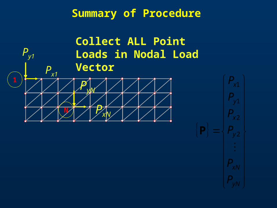
Collect ALL Point Loads in Nodal Load Vector

yN

xN

y

x

y

x

P

P

P

P

P

P

2

2

1

1

P

1

N

Px1

Py1

PxN

PyN

Summary of Procedure

Form Stiffness Equations

e

ekK

PTfF e

ee

nT qqq 21Q

nT FFF 21F

KQF

Summary of Procedure

eeee qBDσ

KQF Apply Boundary Conditions

Solve FKQ 1

For Every Element Compute Stress

Example

(0,0) (3,0)

(3,2)(0,2)Tt=200 lb/in

fx=0

fy=60 lb/in2

ANSYS Solution – Coarse Mesh

2-D Constant Stress Triangle

• First Element for Stress Analysis

• Does not work very well

• When in Bending under-predicts displacements– Slow convergence for fine mesh

• For in plane strain conditions – Mesh “Locks”– No Deformations

Comments

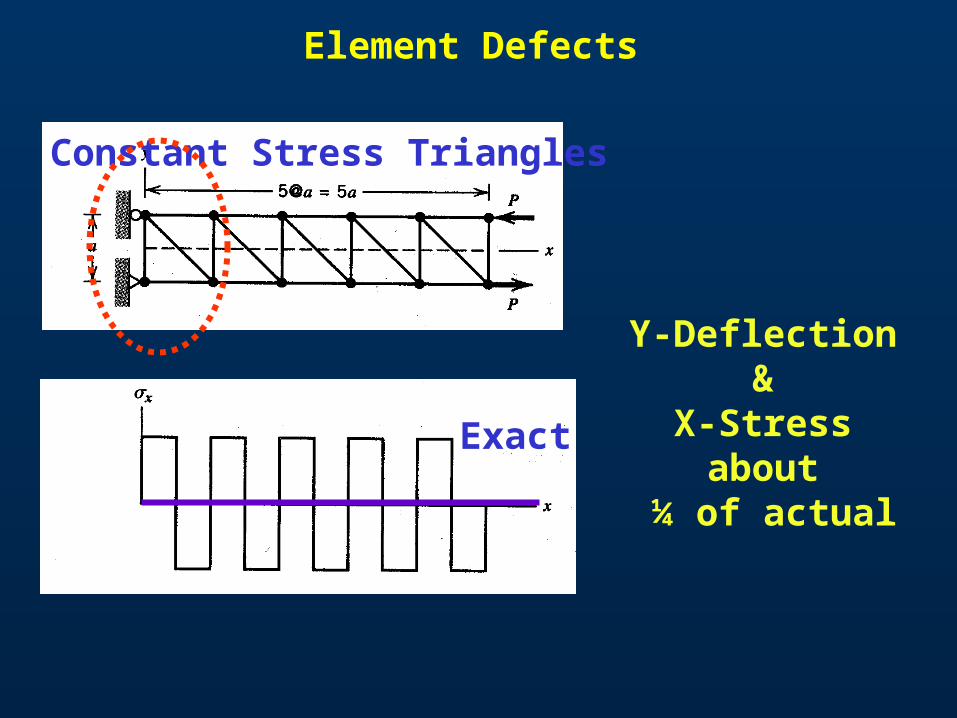
Element Defects

Element Defects

Constant Stress Triangles

Exact

Y-Deflection &X-Stress about

¼ of actual

Element Defects

0

0

0

0

011

011

1000

10

0001

01

2

2

v

u

aaaa

aa

aa

xy

y

x

x1=0, y1=0 x2=a, y2=0 x3=0, y3=a

a

ux

2

0y

a

uxy

2 ?Spurious Shear Strain Absorbs Energy – Larger Force Required

Element Defects

Mesh Lock

Rubber Like Material ~0.5