earthquake engineering at berkeley - ed wilsonedwilson.org/history/earthquake engineering at...

1 Journal Information © 2005 Springer. Printed in the Netherlands.

EARTHQUAKE ENGINEERING AT BERKELEY

From the Proceedings of NATO ARW, Opattia, Croatia, 2006

THE HISTORY OF EARTHQUAKE ENGINEERING AT THE

UNIVERSITY OF CALIFORNIA AT BERKELEY AND RECENT

DEVELOPMENTS OF NUMERICAL METHODS AND COMPUTER

PROGRAMS AT CSI BERKELEY

EDWARD L. WILSON Professor Emeritus of Structural Engineering University of California at Berkeley 1050 Leneve Place, El Cerrito, CA 94530 USA

Abstract. The purpose of this paper is to summarize, from a personal viewpoint, some research in structural dynamics within the Department of Civil Engineering at the University of California at Berkeley during the period of 1950 to 1990. The second part of the paper is to present a few recently developed numerical algorithms for dynamic analysis that are required in the design of wind, wave and earthquake resistant structures. These algorithms have been incorporated into the SAP 2000 programs (developed by Computers and Structures, Inc. in Berkeley) and have been used in the analysis of hundreds of large structural systems. This most recent research and development work was conducted since the author’s retirement in1991 from teaching at the University.

Keywords: Earthquakes; Eigenvalues; Error Analysis; Static Vectors; Termination of LDR Vectors, Fast Nonlinear Analysis; Periodic Loading; Graduate Study at Berkeley,

EARTHQUAKE ENGINEERING AT BERKELEY 2

1. Structural Dynamics Research at UC Berkeley 1950 to 1990

1.1. INTRODUCTION

The University of California was established in 1868 and was authorized to teach courses in several different disciplines, including Military Science and Civil Engineering, CE. At that time the other engineering disciplines did not exist. By the time this author started his undergraduate work in early nineteen fifty the undergraduate courses in dynamics were conducted by faculty members from the department of Mechanical Engineering, with emphasis on rigid body dynamics.

The Building Codes that were used in structural engineering design courses for buildings and bridges did not contain the words earthquake or seismic forces. Also, the majority of the structural engineering faculty at Berkeley did not seem to be concerned about the effects of dynamic loading.

In 1949 Professor Ray Clough joined the CE faculty and began teaching a graduate structural dynamics course for students in CE and the Naval Architecture departments. Clough had also been a weather officer in the US Army Air Corps during WWII and had developed an appreciation of natural disasters.

In 1953 Professor Joseph Penzien joined the CE faculty3. Both Ray and Joe had received their undergraduate degrees from the University of Washington and their Doctors’ degrees from Massachusetts Institute of technology. In addition, both had extensive practical experience with the analysis of aircraft structures and blast analysis of all types of structures. They appeared to have a similar educational and practical background; however, their approach to the solution of dynamic problems was often very different. Their collaboration during the next 25 years resulted in the publication of the classical textbook Dynamics of Structures in 1975. In 2003, the latest edition of the book was reprinted and can be obtained from CSI in Berkeley1.

During the early nineteen fifties very little research funding was available for research in the area of structural dynamics. Therefore, both Clough and Penzien were forced to take summer employment at companies, such as Boeing, and to work for local engineering firms as consultants.

However, during the late nineteen fifties and early nineteen sixties funded research projects increased significantly for the following reasons:

First; the CE faculty members hired during the twenty years after World War II were young and energetic with excellent practical experience and impressive educational backgrounds. Also, the majority of the new faculty was capable of conducting both experimental and theoretical research.


3

Second; the introduction of the digital computer required that new numerical analytical methods be developed. The early work of Professor Clough in the creation of the Finite Element Method is an example of a new method that revolutionized many different fields in engineering and applied mathematics.

Third; the Federal Government and the California Department of Transportation were rapidly expanding the freeway system in the state and were sponsoring research at Berkeley, led by Professors Scordelis and Monismith, concerning the behavior of bridges and overpass structures.

Fourth; it was the height of the Cold War and the Defense Department was studying the cost and ability to reinforce buildings and underground structures to withstand nuclear blasts.

Fifth; the manned space program was a national priority. Professors Pister, Penzien, Popov, Sackman, Taylor and Wilson were very active conducting research related to these activities.

Sixth; the offshore drilling for oil in deep water and the construction of the Alaska pipeline required new technology for steel structures, which was developed by Professors Popov, Bouwkamp and Powell.

Finally; after the 1964 Alaska earthquake (and small tsunami that hit northern California) the National Science Foundation initiated a very significant program on Earthquake Engineering Research.

To support this research and development a new Structural Engineering Building, Davis Hall, was completed in 1968 on the Berkeley campus and a large shaking table, to simulate earthquake motions, was constructed at the Richmond Field Station (1971).

1.2. THE EARTHQUAKE ENGINEERING RESEARCH CENTER

Professors Penzien and Clough wrote a formal proposal to the University requesting the creation of the Earthquake Engineering Research Center, EERC. The proposal was approved by the University Administration and Professor Penzien was named as the first director of the Center in December 1967.

EERC was approved as an Organized Research Unit, ORU; however, the center was not given a budget. Therefore, Professors Penzien, Clough and many other members of the UC faculty spent a significant amount of time, in addition to their normal teaching responsibilities, to obtain more permanent funding for the Center. During the first several years of EERC the National Science Foundation provided a significant amount of the funding for the Center and the construction of the world’s largest shake table.


1.3. IMPACT ON THE STRUCTURAL ENGINEERING ACADEMIC PROGRAM

The existence of EERC and the pioneering Finite Element Research Programs in the Division of Structural Engineering and Structural Mechanics, SESM, within the Department of Civil Engineering, made the Graduate Program at Berkeley very popular. The finite element research was complimented by the unique and modern dynamic experimental facilities at EERC.

The SESM program attracted a very large number of bright national and international students. In addition, many post doctoral research scholars and faculty members from other universities spent one or more years at Berkeley.

1.4. WORKING UNDER THE DIRECTION OF PROFESSOR CLOUGH

In 1960 -63 the author, as a doctoral student working under the supervision of Professor Ray Clough, developed the first fully automated finite element program for two-dimensional plane structures. Also, several other students working with Professor Clough extended the program to include the effects of nonlinear material crack closing and creep. In addition to completing a Doctor’s degree with Professor Clough, the author had the opportunity to assist him with consulting activities involving the earthquake and blast response analysis of many different buildings and bridges.

1.5. EXPERIENCE WORKING IN THE AEROSPACE PROGRAM

The author worked as a Senior Development Engineer at Aerojet General Corporation in Sacramento, CA during the period 1963 to 1965. He was responsible for the development of numerical methods and computer programs for the structural analysis of the Apollo spacecraft and other rocket components. The experience was very frustrating since engineers were not allowed to conduct dynamic analysis if they were assigned to a static analysis group. However, the author did learn that it was possible to design elastic structures to withstand forces greater that ten times the force of gravity. In August 1965 the author returned to UC Berkeley as an Assistant Professor of Structural Engineering.

1.6. THE SAP SERIES OF COMPUTER PROGRAMS

In the mid and late nineteen sixties, many different Universities and companies were working on general purpose programs which assumed that each joint has six displacement degrees of freedom (three displacements and


5

three rotations). In general, most of these programs were developed by groups of ten or more engineers and programmers.

In 1969 the Author realized that it was possible to develop a general purpose Structural Analysis Program4 (SAP) that was simple and efficient. The key to the simplicity of SAP was to create, within the program, an equation ID array dimensioned 6 by the number of joints (nodes). The boundary conditions and the type of elements connected to each joint determined if an equilibrium equation existed. Therefore, the stiffness matrix could be directly formed in a compact form. The majority of the program was written by the Author. Five graduate students, working part-time, incorporated several different elements from previously written special purpose programs. The total time required for the program development was less than a man-year. The development was funded with small grants from local structural engineering companies. The three-dimensional solid element was sponsored by the Walla Walla District of the Corps of Engineers. The first version of SAP3 was released within a year (1970). The dynamic response was based on the automatic generation of one set of Ritz vectors. At the time of release it was the fastest and largest capacity structural analysis program of its time.

Development of SAP continued for the next few years with sponsorship from users of the program. Dr. Klaus Jürgen Bathe was responsible for the final version of the program6, SAP IV, in 1972. Dr. Bathe incorporated his ‘Subspace Iteration Algorithms” for the evaluation of the exact eigenvalues and vectors of very large structural systems5. In addition, he was responsible for documentation and international distribution of the program.

In addition, Dr. Bathe developed a completely new static and dynamic computer analysis program, NONSAP7. It was designed to solve general structures with nonlinear material, large strains and large displacements. Later at MIT Professor Bathe continued this research and developed the ADINA program.

All computer programs developed during this early period at Berkeley were freely distributed worldwide, allowing practicing engineers to solve many new problems in structural dynamics. Hence, the research was rapidly transferred to the engineering profession. In many cases the research was used professionally prior to the publication of a formal paper.

Regarding the distribution of the FORTRAN programs from the University, it was made clear that the programs were not to be resold. However, this was not the case. Many companies and other Universities created, distributed and sold modified versions of the program. In addition, some obtained government funding to modify the UC programs. At the same time, proposals by this author


to NSF for research on numerical methods for dynamic analysis were not funded

1.7. RESEARCH AT UC DURING THE NINETEEN EIGHTIES

The author had several excellant doctoral students during the nineteen eighties that worked on many important problems in computational mechanics, incremental construction, dam-reservoir interaction, parallel processing and structural dynamics. One of the most significant accomplishments during the period was proving that the exact dynamic eigenvalues and vectors were not the best basis for performing dynamic analysis by the mode superposition method 8,9,10,11. It was shown that Load Dependent Ritz vectors could be generated by a simple algorithm that was faster than the subspace iteration algorithm and always produced more accurate results than the use of the exact eigenvalues and vectors.

1.8. THE INTRODUCTION OF THE INEXPENSIVE PERSONAL COMPUTER

On a leave from the University, in 1980 the author purchased an inexpensive ($6,000) personal computer with the CPM operating system. It had a FORTRAN compiler; however, it had only 64k of 8 bit high-speed memory and limited low-speed disk storage. Therefore, it was impossible to move large mainframe programs to these small personal computers. However, it was an opportunity to write a completely new general purpose structural analysis program that would incorporate the latest research in finite element technology and numerical methods that had been developed since the release of SAP IV in 1973. The most significant changes was in the dynamic analysis method where Load Dependant Ritz (LDR) modal vectors8 were introduced as and option.

The small amount of high-speed memory on the first personal computers required that a structural analysis program be subdivided into separate program modules which were executed in sequence via batch files. For example, the preprocessing, formation of each different type of element stiffness matrix, the assembly of the global stiffness matrix, solution of equation, solution for eigenvalues, integration of modal equations, calculation of element forces plotting and post processing were all separate programs. Therefore, the first version of SAP 80 was very easy to develop and maintain. Also, it automatically had a restart option. In order to avoid a conflict of interest with his research at the University, the author did not use one line of code from SAP IV and personally did all the SAP 80 development work at his home office on his personal computer.


7

After the release of the 16 bit IBM personal computer in 1983 with 64 bit floating point hardware, large capacity hard disks, and a standard colored graphics terminal, it was possible to solve large practical structural systems. At this point in time it was apparent that the development of SAP80 required additional staff. The author made an agreement with a former UC student, Ashraf Habibullah president of Computers and Structures, Inc. (CSI), to add design options and graphical pre and post processors to SAP 80 in order that it would better serve the needs of the structural engineering profession and to provide professional support to the users of the program. This association with CSI has continued for nearly 25 years and has been very successful in the transfer of the latest research to the structural engineering profession. In addition, CSI has created a special purpose program of SAP2000 for multistory buildings, ETABS, This program has special pre and post processing capabilities and automatic design options for earthquake engineering.

2. Research and Development at CSI to Present

2.1. SAP 90 AND SAP 2000

In 1990 the Author had a mild heart attack and decided to retire from teaching at the University and work at a more leisurely pace with CSI on the development of the next version of the program, SAP 90. A new improved SOLID element, three degrees of freedom per node, and a new thin or thick shell element, six degrees of freedom per node, were implemented.

By 1990 the earthquake engineering profession was beginning to use nonlinear base isolation and energy dissipation devices to reduce the response, and damage, of structures to earthquake motions. Therefore, there was a strong motivation to add this option to SAP 90.

The approach used to solve this class of nonlinear problems was to move the nonlinear force associated with these elements to the right hand side of the node point equilibrium equations; then, solve the uncoupled modal equations by iteration as the mode equations are integrated11. Since the nonlinear forces are treated as external loads, LDR vectors must be generated for each of these nonlinear degrees of freedom. This new approach is named the Fast Nonlinear Analysis, FNA, method.

2.2. EXAMPLES OF NONLINEAR ELEMENTS

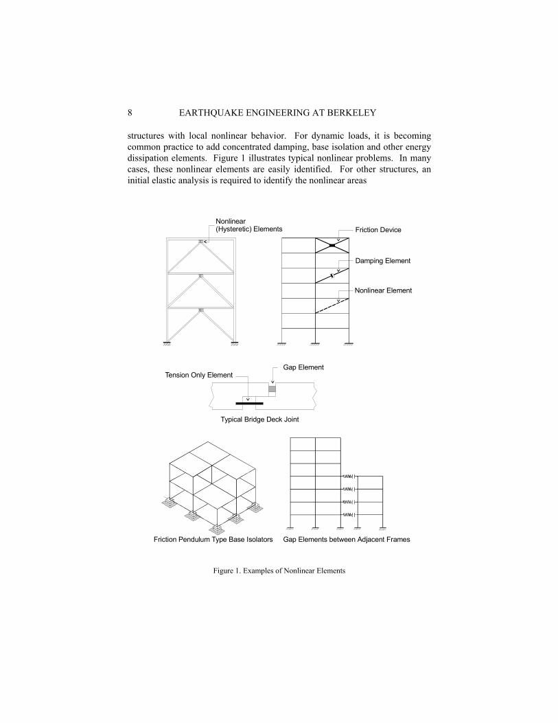
Local buckling of diagonals, uplifting at the foundation, contact between different parts of the structures and yielding of a few elements are examples of


F r i c t i o n D e v i c e

D a m p i n g E l e m e n t

N o n l i n e a r E l e m e n t

G a p E l e m e n t T e n s i o n O n l y E l e m e n t

T y p i c a l B r i d g e D e c k J o i n t

F r i c t i o n P e n d u l u m T y p e B a s e I s o l a t o r s G a p E l e m e n t s b e t w e e n A d j a c e n t F r a m e s

N o n l i n e a r ( H y s t e r e t i c ) E l e m e n t s

structures with local nonlinear behavior. For dynamic loads, it is becoming common practice to add concentrated damping, base isolation and other energy dissipation elements. Figure 1 illustrates typical nonlinear problems. In many cases, these nonlinear elements are easily identified. For other structures, an initial elastic analysis is required to identify the nonlinear areas

Figure 1. Examples of Nonlinear Elements


9

After several years experience with the application of the FNA method on hundreds of large structural systems, it was found that the method could fail if there was very small or no mass associated with the nonlinear force. Therefore, it was necessary to modify the LDR vector algorithm in order that certain static vectors are included in the FNA method.

3. New Load Dependent Ritz Vector Algorithm and Error Analysis

3.1. THE COMPLETE EIGENVALUE SUBSPACE

In the analysis of structures subjected to three base accelerations there is a requirement that one must include enough modes to account for 90 percent of the mass in the three global directions. However, for other types of loading, such as base displacement loads and point loads, there are no guidelines as to how many modes are to be used in the analysis. In many cases it has been necessary to add static correction vectors to the truncated modal solution in order to obtain accurate results. One of the reasons for these problems is that number of eigenvectors required to obtain an accurate solution is a function of the type of loading that is applied to the structure. However, the major reason for the existence of these numerical problems is that all the LDR vectors of the structural system are not included in the analysis.

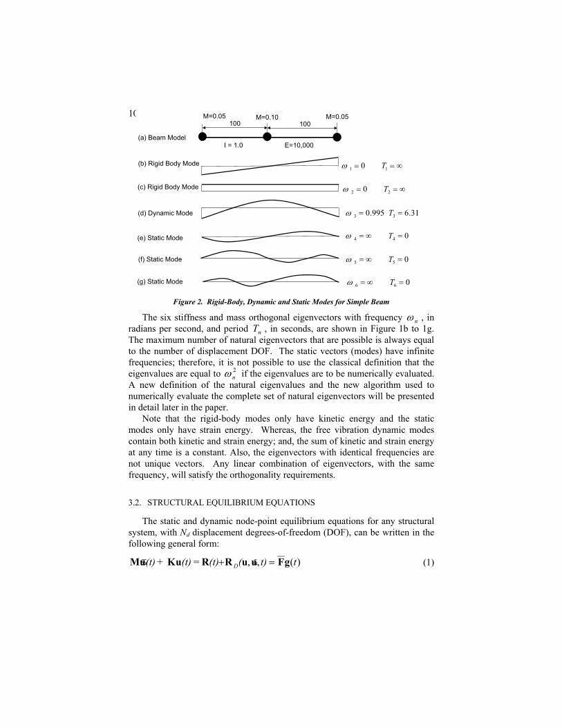
In order to illustrate the physical significance of the complete set of LDR vectors for a structure consider the unsupported beam shown in Figure 1a. The two-dimensional structure has six displacement DOF, three rotations (each with no rotational mass) and three vertical displacements (each with a vertical lumped mass).


Figure 2. Rigid-Body, Dynamic and Static Modes for Simple Beam

The six stiffness and mass orthogonal eigenvectors with frequency nω , in radians per second, and period nT , in seconds, are shown in Figure 1b to 1g. The maximum number of natural eigenvectors that are possible is always equal to the number of displacement DOF. The static vectors (modes) have infinite frequencies; therefore, it is not possible to use the classical definition that the eigenvalues are equal to 2

nω if the eigenvalues are to be numerically evaluated. A new definition of the natural eigenvalues and the new algorithm used to numerically evaluate the complete set of natural eigenvectors will be presented in detail later in the paper.

Note that the rigid-body modes only have kinetic energy and the static modes only have strain energy. Whereas, the free vibration dynamic modes contain both kinetic and strain energy; and, the sum of kinetic and strain energy at any time is a constant. Also, the eigenvectors with identical frequencies are not unique vectors. Any linear combination of eigenvectors, with the same frequency, will satisfy the orthogonality requirements.

3.2. STRUCTURAL EQUILIBRIUM EQUATIONS

The static and dynamic node-point equilibrium equations for any structural system, with Nd displacement degrees-of-freedom (DOF), can be written in the following general form:

)(,, = + tt)((t)(t)(t) D gFuuRRuKuM =+ &&& (1)

∞== 11 0 Tω

(a) Beam Model

(b) Rigid Body Mode

(c) Rigid Body Mode

(d) Dynamic Mode

(e) Static Mode

(f) Static Mode

(g) Static Mode

100 100

I = 1.0 E=10,000

M=0.05 M=0.10 M=0.05

∞== 22 0 Tω

31.6995.0 33 == Tω

044 =∞= Tω

055 =∞= Tω

066 =∞= Tω


11

At time t the node acceleration, velocity, displacement and external applied load vectors are defined by (t)(t)t(t) Ruuu and ),(, &&& , respectively.

The unknown force vectors, t)(D ,,uuR & , are the forces associated with internal energy dissipation such as damping and nonlinear forces. In most cases, these forces are self-equilibrating and do not contribute to the global equilibrium of the total structure.

The sum of R and DR can always be represented by the product )(tgF , where F is an Nd by L matrix of L linearly independent spatial load vectors associated with both linear and nonlinear behavior, and )(tg is a vector of L time functions. These time functions are directly specified for linear analysis, and are evaluated by iteration for nonlinear elements. For many problems, nonlinear forces may be restricted to a subset of all DOF, so that dNL < , although this is not required in what follows.

The node-point lumped mass matrix, M , need not have mass associated with all degrees-of-freedom; therefore, it may be singular and mathematically positive semi-definite. Also, external loads may be applied to displacement DOF that do not have mass and produce only static displacements.

The linear elastic stiffness matrix K may contain rigid-body displacements, as is the case for ship and aerospace structures; therefore, it need not be positive-definite. In order to overcome this potential singularity the term

(t)uMρ may be added to both sides of the equilibrium equations, where ρ is an arbitrary positive number. Or, Equation (1) can be written as

(t) = + RuMFguKuM =+ (t)(t)(t)(t) ρ&& (2)

While K and M may be singular, it is assumed here that the effective-stiffness matrix, MKK ρ+= , is nonsingular. Therefore, the effective-stiffness matrix represents a real structure with the addition of external springs to all mass DOF; these springs have stiffness proportional to the mass matrix.

The purpose of this paper is to present a general solution method for the numerical calculation of displacement and member forces. The proposed method can be used for both static and dynamic loads and has the ability to include arbitrary damping and nonlinear energy dissipation. The derivation of the vector-generation algorithm presented in this paper is self-contained and only uses the fundamental laws of physics and mathematics. Near the end of the paper, it will be pointed out that each step in the solution algorithm is nothing more than the application of well-known numerical techniques that have existed for over fifty years. It is an extension of Load Dependent Ritz vectors that have been previously described Wilson, 2003.


3.3. CHANGE OF VARIABLE

Equation (2) is an exact equilibrium statement for the structure at all points in time. The first step in the static or dynamic solution of this fundamental equilibrium equation is to introduce the following change of variable:

(t)(t) ΦYu = and (t)(t) YΦu &&&& = (3)

The Nd by N matrix Φ of spatial vectors are calculated and normalized to satisfy the following orthogonality equations:

ΨMΦΦ =T (4)

or, ΨIKΦΦIΦKΦ ρ−== TT (5)

The N by N diagonal matrices are I for the unit matrix and Ψ for the generalized mass matrix associated with each vector. Therefore, Equation (2) can be written as a set of uncoupled equations of the following form:

)( = + T t(t)(t) RΦYIYΨ && (6)

If N equals Nd , the introduction of this simple change of variables into Equation (2) does not introduce any additional approximations. The number of nonzero terms in the diagonal matrix Ψ indicates the maximum number of dynamic vectors and is equal to the number of lumped masses in the system (or, mathematically, the rank of the mass matrix). If a vector has zero generalized mass it indicates that it is a static response vector.

It is not practical to calculate all Nd static and dynamic shape functions for a large structure. First, it would require a large amount of computer time and storage. Second, a large number of vectors that are not excited by the loading may be calculated. Therefore, a truncated set of N natural eigenvectors will be calculated that will produce an accurate solution for an optimum number of LDR vectors.

In order to minimize the number of shape functions required to obtain an accurate solution the static displacement vectors produced by L linearly independent spatial functions )1(F associated with the loading )(tR will be used to generate the first set of vectors. The linear independent spatial load functions )1(F can be automatically extracted from )(tR based on the type of external global loading and the location of the nonlinear elements.


13

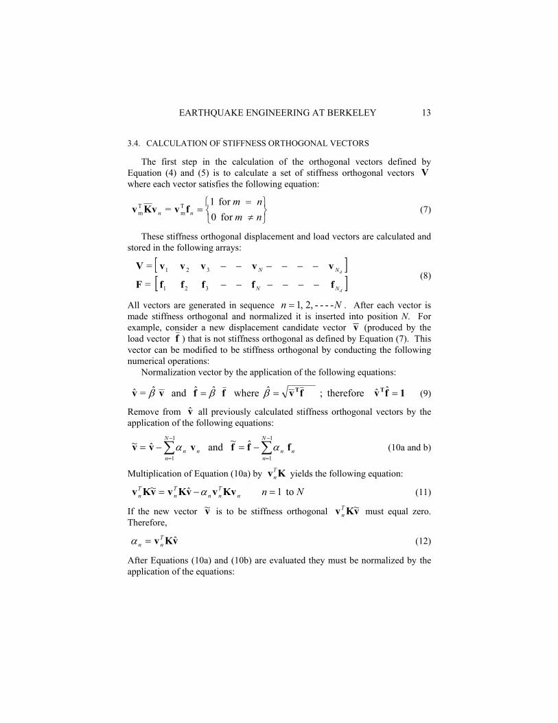
3.4. CALCULATION OF STIFFNESS ORTHOGONAL VECTORS

The first step in the calculation of the orthogonal vectors defined by Equation (4) and (5) is to calculate a set of stiffness orthogonal vectors V where each vector satisfies the following equation:

≠=

=nm nm

nn for 0for 1

= Tm

Tm fvvKv (7)

These stiffness orthogonal displacement and load vectors are calculated and stored in the following arrays:

[ ][ ]

d

d

NN

NN

fffffF

vvvvvV

−−−−−−

−−−−−−

321

321

=

= (8)

All vectors are generated in sequence Nn ---- ,2,1= . After each vector is made stiffness orthogonal and normalized it is inserted into position N. For example, consider a new displacement candidate vector v (produced by the load vector f ) that is not stiffness orthogonal as defined by Equation (7). This vector can be modified to be stiffness orthogonal by conducting the following numerical operations:

Normalization vector by the application of the following equations:

1fvfvffvv TT === ˆˆ e therefor; ˆ whereˆˆ and ˆ =ˆ βββ (9)

Remove from v̂ all previously calculated stiffness orthogonal vectors by the application of the following equations:

ˆ~ and ˆ~ 1

1

1

1∑∑−

=

−

=

−=−=N

nnn

N

nnn fffvvv αα (10a and b)

Multiplication of Equation (10a) by KvTn yields the following equation:

NnnTnn

Tn

Tn to1ˆ~ =−= KvvvKvvKv α (11)

If the new vector v~ is to be stiffness orthogonal vKv ~Tn must equal zero.

Therefore,

ˆ vKvTnn =α (12)

After Equations (10a) and (10b) are evaluated they must be normalized by the application of the equations:


1fv

fvffvv T

=

==

NTN

NN

therefore

; ~~ where~ and ~ = βββ (13)

It is now possible to check if the candidate vector v was linearly independent of the previously calculated vectors by checking if the proposed new vector Nv is nothing more than numerical round-off. Therefore,

vector orthogonal stiffness new a as reject If Nvtol<β (14)

The value for tol is selected to be approximately 10-7. The first block of candidate vectors is obtained by solving the following set

of equations, where the static loads )1(F and displacements )1(V are Nd by L matrices:

)1()1()1( = FVLDLVK T = (15)

Note that the effective stiffness matrix need be triangularized, TLDLK = , only once. Additional blocks of candidate vectors can be generated from the solution of the following recursive equation:

)()1()( = iii FVMVK =− (16)

If, during the orthogonality calculation, a new displacement or load vector in the block is identified as the same (parallel) as a previously calculated vector it can be discarded from the block and the algorithm is continued with a reduced block size. If the block size is reduced to zero, prior to the production of Nd vectors, it indicates that all of the static and dynamic vectors, excited by the initial load patterns, have been found.

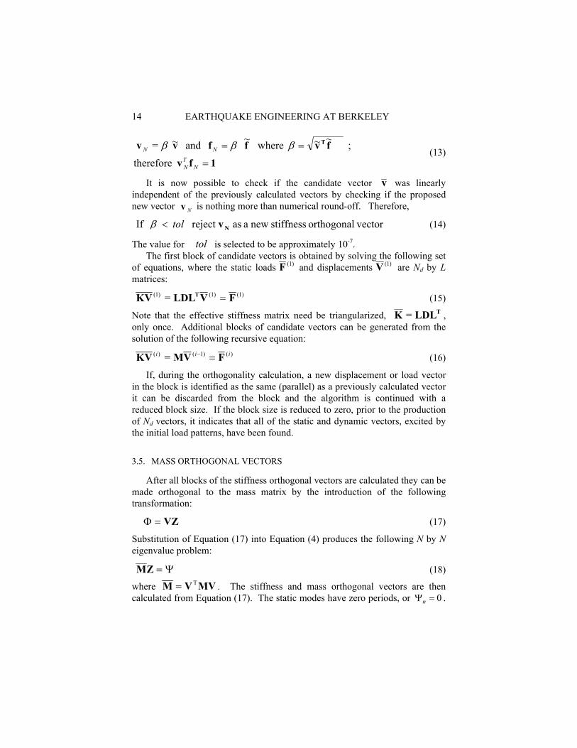
3.5. MASS ORTHOGONAL VECTORS

After all blocks of the stiffness orthogonal vectors are calculated they can be made orthogonal to the mass matrix by the introduction of the following transformation:

VZ=Φ (17)

Substitution of Equation (17) into Equation (4) produces the following N by N eigenvalue problem:

Ψ=ZM (18)

where MVVM T= . The stiffness and mass orthogonal vectors are then calculated from Equation (17). The static modes have zero periods, or 0=Ψn .


15

Therefore, in order to avoid all potential numerical problems, it is recommended that the classical Jacobi rotation method2 be used to extract the eigenvalues and vectors of this relatively small eigenvalue problem.

Equation (2) can now be rewritten as

(t)(t)(t)(t) FguMuKuM = + ρ−&& (19)

The transformation to modal coordinates produces the following uncoupled model equations:

)( =][ + t(t)(t) T FgΦYΨIYΨ ρ−&& (20)

Therefore, a typical modal equation, n, can be written as

)( =][1 + t(t)Y(t) Y Tnnnnn Fgφρ Ψ−Ψ && (21)

The number of static shape functions is equal to the number of zero diagonal terms in the matrix Ψ . For the static modes nΨ is equal to zero and the solution is written as

)( = t(t)Y Tnn Fgφ (22)

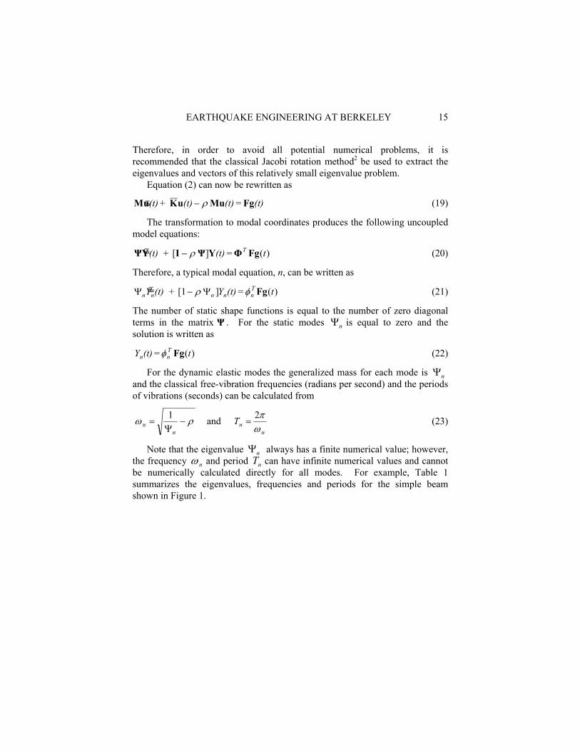
For the dynamic elastic modes the generalized mass for each mode is nΨ and the classical free-vibration frequencies (radians per second) and the periods of vibrations (seconds) can be calculated from

nn

nn T

ωπρω 2 and 1

=−Ψ

= (23)

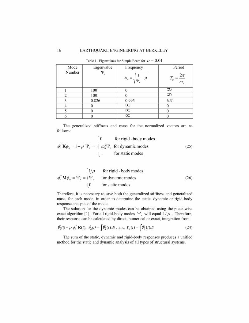
Note that the eigenvalue nΨ always has a finite numerical value; however, the frequency nω and period nT can have infinite numerical values and cannot be numerically calculated directly for all modes. For example, Table 1 summarizes the eigenvalues, frequencies and periods for the simple beam shown in Figure 1.


Table 1. Eigenvalues for Simple Beam for 01.0=ρ

Mode Number

Eigenvalue nΨ

Frequency

1ρω −

Ψ=

nn

Period

nnT

ωπ2 =

1 100 0 ∞ 2 100 0 ∞ 3 0.826 0.995 6.31 4 0 ∞ 0 5 0 ∞ 0 6 0 ∞ 0

The generalized stiffness and mass for the normalized vectors are as

follows:

=Ψ−= nnTn ρφφ 1K

Ψmodes staticfor 1

modes dynamicfor modesbody -rigidfor 0

2n nω (25)

Ψ=Ψ=

modes staticfor 0modes dynamicfor

modesbody -rigidfor 1

nnnTn

ρφφ M (26)

Therefore, it is necessary to save both the generalized stiffness and generalized mass, for each mode, in order to determine the static, dynamic or rigid-body response analysis of the mode.

The solution for the dynamic modes can be obtained using the piece-wise exact algorithm [1]. For all rigid-body modes nΨ will equal ρ/1 . Therefore, their response can be calculated by direct, numerical or exact, integration from

∫ ∫== dttYtYdttY(t)Yt(t)Y nnnnTnn )()( and , )( ,)( = &&&&&& Rφρ (24)

The sum of the static, dynamic and rigid-body responses produces a unified method for the static and dynamic analysis of all types of structural systems.


17

3.6. MATHEMATICAL CONSIDERATIONS

Except for reference to the Jacobi and piece-wise integration methods2 Wilson, 2003, the numerical method for the generation of stiffness and mass orthogonal vectors presented is based on the fundamentals of mechanics and requires no additional references to completely understand. However, it is very interesting to note that the method is nothing more than the application of several well-known numerical techniques:

First, the change of variables introduced by Equation (3) is an application of the standard method of solving differential equation and is also known as the separation of variables in which the solution the solution is expressed in terms of the product of space functions and time functions. A special application of this approach in classical structural dynamics is called the mode superposition method in which the static mode response is neglected.

Second, the addition of the term (t)uMρ to the stiffness matrix is called an eigenvalue shift in mathematics. However, it is worth noting the zero eigenvalues associated with the static modes are not shifted.

Third, the recurrence relationship, Equation (10), is identical to the inverse iteration algorithm for a single vector2. Therefore, the approach is a power method that will always converge to the lowest eigenvalues of the system.

Fourth, the series of vectors generated by the inverse iteration method is known as the Krylov Subspace . A. N. Krylov, 1863-1945, was a well-known Russian engineer and mathematician who first studied the dynamic response of ship structures. However, Krylov did not include static modes in his work.

Fifth, orthogonality is maintained, Equations (14), by the application of the modified Gram-Schmidt algorithm. Theoretically, after the initial block of orthogonal vectors are calculated, it is only necessary to make each new displacement vector orthogonal with respect to the previous two Krylov vectors. However, after many years of experience with the dynamic analysis of very large structural systems, we have found that it is necessary to apply the Gram-Schmidt method to all previously calculated vectors in order that the same vectors are not regenerated.

Sixth, the performance of the algorithm is improved if the load vectors )( iF , for each block, are made orthogonal with respect to the previously

calculated displacement vectors, Equation (16), prior to the solution of the equilibrium equations. This additional step has made the algorithm unique and very robust.


3.7. LOAD PARTICIPATION RATIOS AND ERROR ESTIMATION

In the analysis of structures subjected to three base accelerations there is a requirement that one must include enough modes to account for 90 percent of the mass in the three global directions. However, for other types of loading, such as base displacement loads, there are no guidelines as to how many modes are to be used in the analysis. The purpose of this section is to define two new load participation ratios, which can be calculated during the generation of the LDR vectors, to assure that an adequate number of vectors are used in a subsequent static or dynamic analysis.

From Equation (24), a typical modal equation n for load pattern j, can be written as

Nntg= Y(t) + t)Y jjTnnn

2nnn to1)(( =ΨΨ Fφω&& (27)

The error indicators are based on the two different types of load functions jg(t) . In one case the loads vs. time excite the low frequencies; and, in the

other case the high frequencies are excited.

3.7.1. Static Loads

The first error estimator is a measure of the ability of a truncated set of mode shapes to capture the static response of the structural system. For this case the load function jg(t) is applied linearly from a value of zero at time zero to a value of 1.0 at the end of a very large time interval. Therefore, the inertia terms can be neglected and Equation (27), evaluated at the end of the large time interval, is

Nn= Y jTnnsn

2n to1=Ψ Fφω (28)

Therefore the static mode participation can be written as

Nn= Y n

2n

jTn

nj to1=Ψω

φ F

(29)

From Equation (3) the approximate static displacement response of the structure due to N modes is

Y N

nnjnj ∑

=

=1φu (30)

The approximate strain energy associated with the displacement defined by Equation (30) is


19

∑

∑∑

=

==

Ψ=

Ψ===

N

n n2n

jTn

njn

N

nnnnjn

N

n

Tnnjj

Tjsj YYY E

1

2

2

1

2

1

)(21

21

21

21

ω

φ

φωφφ

F

KuKu (31)

The exact static displacement due to the load pattern can be calculated from the solution of the following static equilibrium equation:

jj FuK = (32)

The exact strain energy stored in the structure for the load pattern is calculated from

E jTjj

Tjsj FuuKu

21

21

== (33)

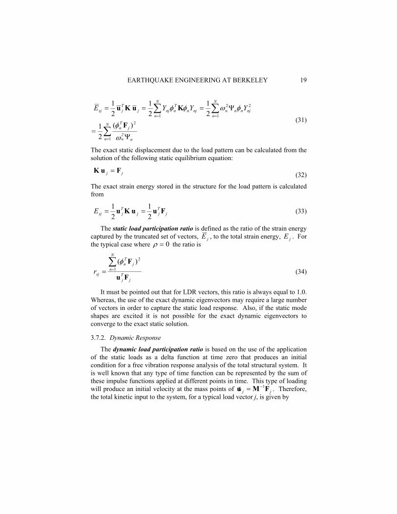
The static load participation ratio is defined as the ratio of the strain energy captured by the truncated set of vectors, jE , to the total strain energy, jE . For the typical case where 0=ρ the ratio is

r j

Tj

N

nj

Tn

sj Fu

F∑== 1

2)(φ (34)

It must be pointed out that for LDR vectors, this ratio is always equal to 1.0. Whereas, the use of the exact dynamic eigenvectors may require a large number of vectors in order to capture the static load response. Also, if the static mode shapes are excited it is not possible for the exact dynamic eigenvectors to converge to the exact static solution.

3.7.2. Dynamic Response

The dynamic load participation ratio is based on the use of the application of the static loads as a delta function at time zero that produces an initial condition for a free vibration response analysis of the total structural system. It is well known that any type of time function can be represented by the sum of these impulse functions applied at different points in time. This type of loading will produce an initial velocity at the mass points of jj FMu 1−=& . Therefore, the total kinetic input to the system, for a typical load vector j, is given by


jTjj

TjkjE FMfuMu 1

21

21 −== && (35)

From Equation (3) the relationship between initial node velocities and the initial modal velocities is

∑=

N

1nn= njj Y&& φu (36)

Therefore, the kinetic energy associated with the truncated set of vectors is

∑=

Ψ==N

nnjnj

Tjkj YE

1

2

21

21 &&& uMu (37)

The initial modal velocity njY& is obtained from the solution of Equation (27) as

n

jTn

njYΨ

=Fϕ& (38)

Substitution of Equation (38) into Equation (37) yields

∑= Ψ

=N

n n

jTn

jkE1

2)(21 Fϕ

(39)

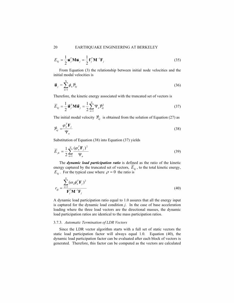
The dynamic load participation ratio is defined as the ratio of the kinetic energy captured by the truncated set of vectors, kjE , to the total kinetic energy,

kjE . For the typical case where 0=ρ the ratio is

r j

Tj

N

nj

Tnn

dj FMF

F

11

2)(

−=∑

=φω

(40)

A dynamic load participation ratio equal to 1.0 assures that all the energy input is captured for the dynamic load condition j. In the case of base acceleration loading where the three load vectors are the directional masses, the dynamic load participation ratios are identical to the mass participation ratios.

3.7.3. Automatic Termination of LDR Vectors

Since the LDR vector algorithm starts with a full set of static vectors the static load participation factor will always equal 1.0. Equation (40), the dynamic load participation factor can be evaluated after each block of vectors is generated. Therefore, this factor can be computed as the vectors are calculated


21

and it can be used as an indicator to automatically terminate the generation of LDR vectors. Based on experience, a dynamic load participation ratio of at least 0.95, for all load patterns, will assure accurate results for most types of loading. This is a very important user option since the number of vectors requested need not be specified prior to the dynamic analysis.

3.8. USE OF THE LDR ALGORITHM TO CALCULATE EIGENVECTORS

The LDR vector algorithm, as presented in this paper, generates the complete Krylov subspace for a specified set of load vectors and errors in the resulting dynamic response analysis are minimized. If one examines the frequencies associated with the LDR vectors it is found that all the lower frequencies are identical to the frequencies obtained from an exact eigenvalue analysis. Since the approach is related to the power method this is to be expected. The higher modes produced by the LDR vector algorithm are linear combinations of the exact eigenvectors and components of the static response vectors. The complete set of LDR vectors is the optimum set of vectors to solve the dynamic response problem associated with the specified static load patterns. Therefore, the number of LDR vectors required will always be less than if the exact eigenvectors were used.

If, for some reason, one wishes to calculate the exact eigenvalues and vectors the same numerical method can be used. The initial displacement vectors need only be set to random vectors. If, during the generation, vectors are generated which are identical to previously calculated vectors they can be replaced with new random displacement vectors. The procedure can be terminated at any time; however, the higher frequencies will not be exact. The introduction of iteration for each block can be used to calculate the exact eigenvalues and vectors. Note that if the system contains M masses, the method will generate M exact eigenvectors; nevertheless, if random load vectors are used directly, instead of )1()( −= ii MVF , the algorithm can continue and will produce Nd-M static response vectors which have infinite frequencies and zero periods.

3.9. SUMMARY OF THE COMPLETE LDR VECTOR ALGORITHM

The use of exact eigenvectors to reduce the number of degrees of freedom required to conduct a dynamic response analysis has significant limitations. The effects of the application of static loads to massless DOF cannot be taken into account. In addition, for certain types of loading a large number of vectors


are required. On the other hand, a large number of exact eigenvectors may be calculated that are not excited by the loading on the structure.

The use of static and dynamic LDR vectors, presented in this paper, eliminates the problems associated with the use of the exact eigenvectors. In addition, the LDR vector algorithm produces a unified approach to the static and dynamic analysis of many different types of structural systems. In addition, it is possible to check if an adequate number of vectors are generated prior to the integration of the equations of motion.

4. The Fast Nonlinear Analysis Method for Seismic Analysis

The FNA method can be applied to both the static and dynamic analysis of linear or nonlinear structural systems. A limited number of predefined nonlinear elements are assumed to exist. Stiffness and mass orthogonal LDR vectors of the elastic structural system are used to reduce the size of the nonlinear system to be solved. The forces in the nonlinear elements are calculated by iteration at the end of each time or load step. The uncoupled modal equations are solved exactly for each time increment.

The computational speed of the new FNA method is compared with the traditional “brute force” method of nonlinear analysis in which the complete equilibrium equations are formed and solved at each increment of load. For many problems the new method is several magnitudes faster.

The response of real structures when subjected to a large dynamic input often involves significant nonlinear behavior. In general, nonlinear behavior includes the effects of large displacements and/or nonlinear material properties.

The use of geometric stiffness and P-Delta analyses includes the effects of first-order large displacements. If the axial forces in the members remain relatively constant during the application of lateral dynamic displacements, many structures can be solved directly without iteration.

The more common type of nonlinear behavior is when the material stress-strain, or force-deformation, relationship is nonlinear. This is because of the modern design philosophy that “a well-designed structure should have a limited number of members which require ductility and that the failure mechanism be clearly defined”. Such an approach minimizes the cost of repair after a major earthquake.

4.1. FUNDAMENTAL EQUILIBRIUM EQUATIONS

The FNA method is a simple approach in which the fundamental equations of mechanics (equilibrium, force-deformation and compatibility) are satisfied.


23

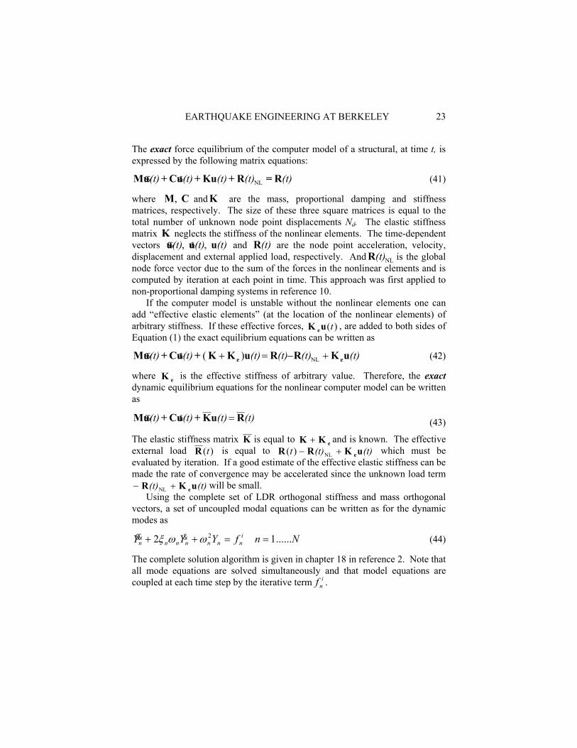
The exact force equilibrium of the computer model of a structural, at time t, is expressed by the following matrix equations:

(t)(t)(t)(t)(t) R = R + Ku + uC + uM NL&&& (41)

where M C, and K are the mass, proportional damping and stiffness matrices, respectively. The size of these three square matrices is equal to the total number of unknown node point displacements Nd. The elastic stiffness matrix K neglects the stiffness of the nonlinear elements. The time-dependent vectors && &u u u(t) (t) (t), , and R(t) are the node point acceleration, velocity, displacement and external applied load, respectively. And NL(t)R is the global node force vector due to the sum of the forces in the nonlinear elements and is computed by iteration at each point in time. This approach was first applied to non-proportional damping systems in reference 10.

If the computer model is unstable without the nonlinear elements one can add “effective elastic elements” (at the location of the nonlinear elements) of arbitrary stiffness. If these effective forces, )(tuK e , are added to both sides of Equation (1) the exact equilibrium equations can be written as

uK RR uKK + uC + uM ee (t)(t)(t)(t)(t)(t) +−=+ NL)(&&& (42)

where eK is the effective stiffness of arbitrary value. Therefore, the exact dynamic equilibrium equations for the nonlinear computer model can be written as

R uK + uC + uM (t)(t)(t)(t) =&&& (43)

The elastic stiffness matrix K is equal to eKK + and is known. The effective external load )(tR is equal to (t)(t)t uK RR e+− NL)( which must be evaluated by iteration. If a good estimate of the effective elastic stiffness can be made the rate of convergence may be accelerated since the unknown load term

(t)(t) uK R e+− NL will be small. Using the complete set of LDR orthogonal stiffness and mass orthogonal

vectors, a set of uncoupled modal equations can be written as for the dynamic modes as

NnfYYY innnnnnn ......12 2 ==++ ωωξ &&& (44)

The complete solution algorithm is given in chapter 18 in reference 2. Note that all mode equations are solved simultaneously and that model equations are coupled at each time step by the iterative term i

nf .


5. Solution for Wind and Wave Loadings

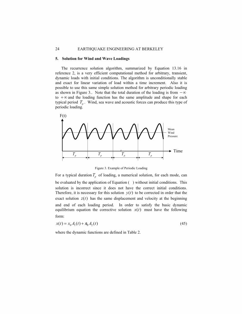
The recurrence solution algorithm, summarized by Equation 13.16 in reference 2, is a very efficient computational method for arbitrary, transient, dynamic loads with initial conditions. The algorithm is unconditionally stable and exact for linear variation of load within a time increment. Also it is possible to use this same simple solution method for arbitrary periodic loading as shown in Figure 3.. Note that the total duration of the loading is from −∞ to +∞ and the loading function has the same amplitude and shape for each typical period Tp . Wind, sea wave and acoustic forces can produce this type of periodic loading.

T

pT pT pT pTTime

F(t)

MeanWindPressure

Figure 3. Example of Periodic Loading

For a typical duration Tp of loading, a numerical solution, for each mode, can

be evaluated by the application of Equation ( ) without initial conditions. This solution is incorrect since it does not have the correct initial conditions. Therefore, it is necessary for this solution y t( ) to be corrected in order that the exact solution z t( ) has the same displacement and velocity at the beginning and end of each loading period. In order to satisfy the basic dynamic equilibrium equation the corrective solution x t( ) must have the following form:

x t x A t x A t( ) ( ) & ( )= +0 1 0 2 (45)

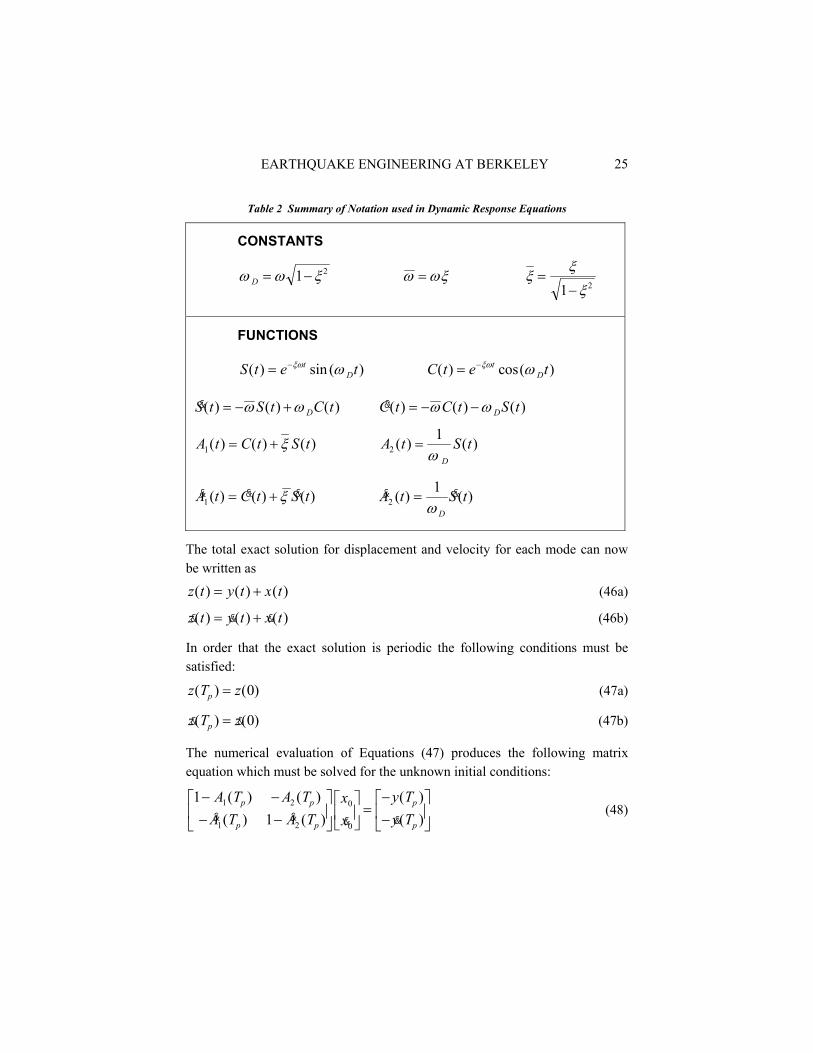
where the dynamic functions are defined in Table 2.


25

Table 2 Summary of Notation used in Dynamic Response Equations

CONSTANTS

ω ω ξD = −1 2 ω ωξ= ξ ξξ

=−1 2

FUNCTIONS

S t e ttD( ) sin ( )= −ξω ω C t e tt

D( ) cos( )= −ξω ω

&( ) ( ) ( )S t S t C tD= − +ω ω &( ) ( ) ( )C t C t S tD= − −ω ω

A t C t S t1( ) ( ) ( )= + ξ A t S tD

21( ) ( )=ω

)()()(1 tStCtA &&& ξ+= )(1)(2 tStAD

&&ω

=

The total exact solution for displacement and velocity for each mode can now be written as

z t y t x t( ) ( ) ( )= + (46a)

&( ) &( ) &( )z t y t x t= + (46b)

In order that the exact solution is periodic the following conditions must be satisfied:

z T zp( ) ( )= 0 (47a)

&( ) &( )z T zp = 0 (47b)

The numerical evaluation of Equations (47) produces the following matrix equation which must be solved for the unknown initial conditions:

11

1 2

1 2

0

0

− −− −

=

−−

A T A TA T A T

xx

y Ty T

p p

p p

p

p

( ) ( )& ( ) & ( ) &

( )&( )

(48)


The exact periodic solution for modal displacements and velocities can now be calculated from Equations (46a and 46b). Hence, it is not necessary to use a frequency domain solution approach for periodic loading as suggested in most textbooks on structural dynamics.

6. Personal Remarks

The majority of the population in the United States has an obsession with the danger of experiencing an earthquake. It is very common to meet someone from the East, South or Midwest, where hurricanes and tornadoes are very common, who states that he or she would not consider living in California because of the fear of earthquakes. However, if one looks at the facts, the fear of earthquakes is not justified.

During the past 500 years fewer than 2,000 people have been killed by

earthquakes in the United States. This figure is extremely small compared to many other typical causes of accidental deaths. The largest causes are automobile crashes (over 30,000 each year), fire, wind and many other types of accidents. In fact, during the past 500 years, several times more people have died in the United States from insect bites than from earthquakes. Also, lightning has killed more people than earthquakes.

Tornadoes and minor flooding are natural disasters that kill hundreds of

individuals each year. However, most of these isolated incidences are not reported by the local or national news media; whereas, a small earthquake in the San Andreas Fault, which measured four on the Richter Magnitude Scale and caused no property damage or personal injuries, is often reported in the national and international press.

Hurricanes Katrina, Rita and Wilma in 2005 devastated New Orleans,

Southern Florida, and the Gulf Coastline killed over 1000 people and significant property damage. In recent years, loss of life from hurricanes has been minimized because the magnitude and time of the hurricane can be predicted. The largest number of fatalities from one hurricane in the US is estimated at 6,000 in Galveston Inland, TX in 1900. In the US wind and floods have caused approximately 100 times more damage and loss of life than earthquakes. However, several times more money is spent on earthquake research than research on the design of wind resistant structures.


27

One cannot disregard, however, that one of the largest recorded natural disasters in recent years was the Tangshan earthquake (Richter Magnitude 7.9) in eastern China in 1976 in which over 600,000 people were killed. During the past 50 years a large number of earthquakes, which have occurred outside the US, have killed over 10,000 people per earthquake. The most recent October 8, 2005 (magnitude 7.6) affected the Kashmir regions of Pakistan and India. Initial estimates are that it killed over 50,000 people. Nearly all these earthquakes have occurred in areas of the world with grossly inadequate design and construction standards. However, the failure of a dam with a large reservoir during an earthquake could cause a large number of fatalities. Or, a large tsunami, generated from an earthquake off the west coast of the US, could kill thousands of people

Most major structures, which are damaged during earthquakes, are designed

by Civil Engineers, who have special training in Structural Engineering. All ground-supported structures are designed in the vertical direction to support their own weight, which is commonly referred to as 1.0g in the vertical direction. The present earthquake design specifications for most structures in the San Francisco Bay Area are less than 50 percent of the weight of the structure or 0.5g applied in the horizontal direction. In aerospace engineering it is common to design structures to carry loads over 10g. Therefore, the common statement, it is not possible to design structures to resist earthquakes, is not true. We have the technology to design earthquake resistant structures and it is an economic decision whether or not to obtain this goal. In addition, earthquake resistant design can place limitations on the architectural form of the structure.

Finally, it is apparent that there is a need to increase funding for applied research and development for wind and coastal engineering. The fundamental research in computational aero and fluid dynamics has been completed. We must create computer programs that are usable by the profession in order to improve the design of structures in wind and coastal areas.


REFERENCES 1. R. W. Clough and J. Penzien, Dynamics of Structures, Computers

and Structures, Inc., 1995 University Avenue, Berkeley, CA, 94704, ISBN 0-923907-50-5, (2003)

2. E. L. Wilson, Three Dimensional Static and Dynamic Analysis of Structures, Computers and Structures, Inc., 1995 University Avenue, Berkeley, CA, 94704, ISBN 0-923907-03-3, (2003).

3. J. Penzien, EERI Oral History Series, 2004

4. E. L. Wilson, SAP A General Structural Analysis Program, Report UCSESM, (September 1970)

5. K. J. Bathe and E. L. Wilson, "Large Eigenvalue Problems in Dynamic Analysis", Proceedings, American Society of Civil Engineers, Journal of the Engineering Mechanics Division, EM6, (December 1972) pp. 1471-1485.

6. K. J. Bathe, K. J., E. L. Wilson and F. E. Peterson, “SAP IV – A Structural Analysis Program ‘, Report EERC 73-11, (June 1973)

7. K. J. Bathe, E. L. Wilson and R. H. Iding, "NONSAP--A Structural Analysis Program for Static and Dynamic Response of Nonlinear Systems" UCB/SESM Report No. 74/3, Berkeley, (February 1974).

8. E. L. Wilson, M. Yuan and J. Dickens, "Dynamic Analysis by Direct Superposition of Ritz Vectors," Earthquake Engineering and Structural Dynamics, Vol. 10, (1982)

9. P. Léger, E. L. Wilson, Clough, R. W. “The Use of Load Dependent Vectors for Dynamic and Earthquake Analysis”. Report UCB/EERC-86/04, Berkeley, (March 1986).

10. K. J. Joo, E. L. Wilson and P. Léger, "Ritz Vectors and Generation Criteria for Mode Superposition Analysis", Earthquake Engineering and Structural Dynamics, Vol.18, pp.149-167.(1989)

11. A. Ibrahimbegovic, H. Chen, E. Wilson and R. Taylor, "Ritz Method for Dynamic Analysis of Large Discrete Linear Systems with Non-Proportional Damping", Earthquake Engineering and Structural Dynamics, Vol. 19, 877-889, 1990.

earthquake engineering at berkeley - ed wilsonedwilson.org/history/earthquake engineering at...

Documents