WDP-154

1154 N~ World Bank Discussion Papers

Earnilngs, Occupati.onalChoi'ce, and Mobi''ityin Segmented LaborMarkets of India

Shahidur R. Khandker

FiLE COPYD

Pub

lic D

iscl

osur

e A

utho

rized

Pub

lic D

iscl

osur

e A

utho

rized

Pub

lic D

iscl

osur

e A

utho

rized

Pub

lic D

iscl

osur

e A

utho

rized

Pub

lic D

iscl

osur

e A

utho

rized

Pub

lic D

iscl

osur

e A

utho

rized

Pub

lic D

iscl

osur

e A

utho

rized

Pub

lic D

iscl

osur

e A

utho

rized

Recent World Bank Discussion Papers

No. 96 Household Food Security and the Role of Women. J. Price Gittinger and others

No. 97 Problems of Developing Countries in the 1990s. Volume I: General Topics. F. Desmond McCarthy, editor

No. 98 Problems of Developing Countries in the 1990s. Volume 11: Country Studies. F. Desmond McCarthy, editor

No. 99 Public Sector Management Issues in Structural Adjustment Lending. Barbara Nunberg

No. 100 The European Communities' Single Market: The Challenge of 1992for Sub-Saharan Africa. Alfred Tovias

No. 101 International Migration and Development in Sub-Saharan Africa. Volume 1: Overview. Sharon Stanton Russell,Karen Jacobsen, and William Deane Stanley

No. 102 International Migration and Development in Sub-Saharan Africa. Volume II: Country Analyses. Sharon Stanton Russell,Karen Jacobsen, and William Deane Stanley

No. 103 Agricultural Extensionfor Women Farmers in Africa. Katrine Saito and C. Jean Weidemann

No. 104 Enterprise Reform and Privitization in Socialist Economies. Barbara Lee andJohn Nellis

No. 105 Redefining the Role of Govemment in Agriculturefor the 1990s. Odin Knudsen,John Nash, and others

No. 106 Social Spending in Latin America: The Story of the 1980s. Margaret E. Grosh

No. 107 Kenya at the Demographic Turning Point? Hypotheses and a Proposed Research Agenda. Allen C. Kelleyand Charles E. Nobbe

No. 108 Debt Management Systems. Debt and International Finance Division

No. 109 Indian Women: Their Health and Economic Productivity. Meera Chatterjee

No. 110 Social Security in Latin America: Issues and Optionsfor the World Bank. William McGreevey

No. 111 Household Consequences of High Fertility in Pakistan. Susan Cochrane, Valerie Kozel, and Harold Alderman

No. 112 Strengthening Protection of Intellectual Property in Developing Countries: A Survey of the Literature. Wolfgang Siebeck,editor, with Robert E. Evenson, William Lesser, and Carlos A. Primo Braga

No. 113 World Bank Lendingfor Small and Medium Enterprises. Leila Webster

No. 114 Using Knowledgefrom Social Science in Development Projects. Michael M. Cernea

No. 115 Designing Major Policy Reform: Lessonsfrom the Transport Sector. Ian G. Heggie

No. 116 Women's Work, Education, and Family Wefare in Peru. Barbara K. Herz and Shahidur R. Khandker, editors

No. 117 Developing Financial Institutionsfor the Poor and Reducing Barriers to Accessfor Women. Sharon L. Holtand Helena Ribe

No. 118 Improving the Performance of Soviet Enterprises. John Nellis

No. 119 Public Enterprise Reform: Lessonsfrom the Past and Issuesfor the Future. Ahmed Galal

No. 120 The Information Technology Revolution and Economic Development. Nagy K. Hanna

No. 121 Promoting Rural Cooperatives in Developing Countries: The Case of Sub-Saharan Africa. Avishay Braverman, J. LuisGuasch, Monika Huppi, and Lorenz Pohlmeier

No. 122 Pe!formance Evaluationfor Public Enterprises. Leroy P. Jones

No. 123 Urban Housing Reform in China: An Economic Analysis. George S. Tolley

No. 124 The New Fiscal Federalism in Brazil. Anwar Shah

No. 125 Housing Reform in Socialist Economies. Bertrand Renaud (Continued on the inside back cover.)

154 ~ 1z1World Bank Discussion Papers

Earnings, OccupationalChoice, and Mobilityin Segmented LaborMarkets of India

Shahidur R. Khandker

The World BankWashiington, D.C.

Copyright e 1992The International Bank for Reconstructionand Development/THE WORLD BANK1818 H Street, N.W.Washington, D.C. 20433, U.S.A.

All rights reservedManufactured in the United States of AmericaFirst printing February 1992

Discussion Papers present results of country analysis or research that is circulated to encourage discussionand comment within the development community. To present these results with the least possible delay, thetypescript of this paper has not been prepared in accordance with the procedures appropriate to formalprinted texts, and the World Bank accepts no responsibility for errors.

The findings, interpretations, and conclusions expressed in this paper are entirely those of the author(s) andshould not be attributed in any manner to the World Bank, to its affiliated organizations, or to members ofits Board of Executive Directors or the countries they represent. The World Bank does not guarantee theaccuracy of the data induded in this publication and accepts no responsibility whatsoever for anyconsequence of their use. Any maps that accompany the text have been prepared solely for the convenienceof readers; the designations and presentation of material in them do not imply the expression of any opinionwhatsoever on the part of the World Bank, its affliates, or its Board or member countries concerning thelegal status of any country, territory, city, or area or of the authorities thereof or concerning the delimitationof its boundaries or its national affiliation.

The material in this publication is copyrighted. Requests for permission to reproduce portions of it shouldbe sent to the Office of the Publisher at the address shown in the copyright notice above. The World Bankencourages dissemination of its work and will normally give permission promptly and, when thereproduction is for noncommercial purposes, without asking a fee. Permission to photocopy portions forclassroom use is not required, though notification of such use having been made will be appreciated.

The complete back]ist of publications from the World Bank is shown in the annual Index of Publications,which contains an alphabetical title list (with full ordering information) and indexes of subjects, authors, andcountries and regions. The latest edition is available free of charge from the Distribution Unit, Office of thePublisher, Department F, The World Bank, 1818 H Street, N.W., Washington, D.C. 20433, U.S.A., orfrom Publications, The World Bank, 66, avenue d'Iena, 75116 Paris, France.

ISSN: 0259-210X

Shahidur R. Khandker is a research economist in the Women in Development Division of the WorldBank's Population and Human Resources Department.

Library of Congress Cataloging-in-Publication Data

Khandker, Shahidur R.Earnings, occupational choice, and mobility in segmented labor

markets of India / Shahidur R. Khandker.p. cm. - (World Bank discussion papers; 154)

Includes bibliographical references.ISBN 0-8213-2062-91. Labor market-India-Bombay. 2. Poor-Employment-India-

-Bombay. 3. Occupational mobility-India-Bombay. 4. Wages-India--Bombay. I. Title. II. Series.HD5820.B6K46 1992331.12'0954'7923-dc2O 92-3419

CIP

Hii

ABSTRACT

This paper, using labor market survey data from Bombay, attempts to identify factors thatdetermine men's and women's earnings, occupational choices, and mobility in segmented labor marketsof India. The paper develops a model that considers three categories of labor-protected wage, unprotectedwage, and self-employment-representing three different forms of labor market segmentation accordingto the type of labor contract and job vulnerability. The results indicate the presence of labor marketsegmentation; however, human capital variables such as education and training have important influenceon both sectoral job allocation and worker's income and occupational mobility. Thus, policies directedto raise the productive capacity and employment levels of the poor may help alleviate poverty.

The labor market outcomes, however, vary by gender. Women are less paid, less mobile, andmore occupied in the unprotected wage sector than men. Men have higher education and so can moreeasily move to the protected wage employment or better remunerated self-employment than womenendowed with lower levels of education. Men have better access to credit than women; thus, self-employed women are more constrained by lack of capital than self-employed men in raising theirproductivity.

Policies such as structural adjustment programs which, inter alia, improve competition, reduceregulatory barriers to employment creation in the protected wage sector, and strengthen fiscal measuresto accelerate growth are perhaps necessary but not sufficient for poverty alleviation. This is because, thesemeasures cannot improve the conditions of the poor, especially women, who are trapped in theunprotected wage sector because of low-levels of education and other forms of human capital. Moretargeted approach is perhaps required. It is therefore necessary to complement structural adjustment byhuman capital development programs that improve productive capacity of the poor as well as institutionstrengthening measures that remove the legal and other regulatory constraints to employment expansionor job mobility. These measures are expected to benefit the poor to gain access to protected wage jobsand also provide an efficient allocation of employment.

iv

ACKNOWLEDGEMENTS

The author wishes to thank Barbara Herz, Dipak Mazumdar, Paul Schultz, Steve Talbot, andseminar participants at World Bank and Harvard University for helpful comments on earlier drafts of thisPaper. John de New provided excellent computer programming and research assistance. Stella Davidprepared the text of this Paper. The author appreciates partial financial support for the Government ofNorway, Ministry of Development Corporation. He is also thankful to the Asian Regional Team forEmployment Promotion (ARTEP) for releasing the Bombay labor market survey data.

v

FOREWORD

Unlike their counterparts in developed nations, women and men in developing countries workmore in the informal sector of the economy where job continuity is uncertain and returns to labor arelow. Women, however, are disproportionately represented in this vulnerable sector. Because jobs in theprotected sector (where job continuity is guaranted by laws) are in short supply relative to demand,personal contacts and "inside" information are important influences on entry to the sector. The result isthat inter-sectoral mobility is restricted for many of the poor, especially women. Research is needed whywomen are so numerous in the unregulated sector, what influences women's inter-sectoral mobility (ifany), and the scope for policy interventions to improve the plight of the poor, including women.

This paper makes an attempt to answer some of these questions using household survey data fromBombay, India. India provides an interesting case study as workers' job vulnerability is not only affectedby economic conditions but also by non-economic influences such as caste and religion. The papersuggests that, although non-economic factors influence market outcomes, policy makers can improveincome and labor mobility of workers, especially women, in the informal sector by investing in theirhuman capital. Poor workers may also gain if the degree of protection granted to the formal sector isreduced.

This paper -- a product of the Women in Development Division, Population and HumanResources Department -- is part of a larger effort in the Bank to determine how women's productivitycan be improved by enhancing their access to education, training, credit, health care, and other publicservices.

Ann 0. HamiltonDirector

Population and Human Resources Department

vii

TABLE OF CONTENTS

1. INTRODUCTION ............................... 1

II. OCCUPATIONAL CHOICES, EARNINGS AND MOBILITY:SEGMENTATION THEORIES REVISITED. 3

III. JOB CHARACTERISTICS AS MEASURE OF MARKETSEGMENTATION AND WORKERS' EARNINGS AND LABORMOBILITY: AN ECONOMIC FRAMEWORK. 5

IV. STUDY AREA AND WORKERS CHARACTERISTICS. 8

V. DETERMINANTS OF EARNINGS IN SEGMENTED LABORMARKETS OF BOMBAY .11Impact of human capital variables .12Impact of worker's background variables .13Impact of job characteristics .13

VI. SECTOR SELECTION AND ITS IMPACT ON WAGES AND LABORSUPPLY BEHAVIOR . ......................................... 14Determinants of sectoral job distribution ............................... 17Sector allocation bias: Test of labor market

segmentation ............................................... 19Determinants of labor supply ........... ........................... 19

VII. DETERMINANTS OF OCCUPATIONAL AND INCOME MOBILITY .... ....... 20Occupational mobility . ......................................... 21Income mobility .............................................. 22

VIII. CONCLUSIONS .23

Bibliography 26

viii

Tables

Table 1. Descriptive Statistics .................................... 29Table 2. Determinants of Protected Wage ................................ 31Table 3. Determinants of Unprotected Wage ............. ................ 32Table 4. Determinants of Hourly Earnings from

Self-employment .33Table 5. Participation Function Estimated by

Multinomial Logit for Male Subsample .34Table 6. Participation Function Estimated by

Multinomial Logit for Female Subsample .35Table 7. Predicted Male Participation by Sample

Characteristics .36Table 8. Predicted Female Participation by Sample

Characteristics .................................... 37Table 9. Employment Function (Hours Worked) Estimation ...... .............. 38Table 10. Censored Regression (Tobit) Estimates of

Occupational Mobility .39Table 11. MNL Estimates of the Determinants of

Occupational Mobility Among theUnprotected Wage Workers 40

Table 12. Random Effects Estimates of Income Mobility ........ .............. 41

Appendices

Table AI. OLS Estimates of Wages/Earnings with SampleSelection Bias Correction .42

Table A2. Employment Function (Hours Worked) EstimationWith Sample Selection Bias Correction .43

Table A3. Probit Estimates of the Determinants ofOccupational Mobility Among the Self-employed .44

Table A4. Probit Estimates of the Determinants ofOccupational Mobility Among the Wage Workers .45

1

I. INTRODUCTION

1.01 Labor market segmentation is an important concern for policymakers in many developingcountries. It produces institutional barriers to the smooth operation of markets, causing inefficiencies thatcan seriously frustrate development. In particular, when the labor market is highly segmented and inter-sectoral labor mobility is restricted, the market process can thwart policies, especially those relying onmarket forces such as structural adjustment programs, that are aimed at alleviating poverty.

1.02 In India, about 25 percent of the population live in urban areas, where 40 percent live belowpoverty level (World Bank 1989). Evidence indicates that many Indian urban workers are trapped intothe unprotected segment of the labor market where the incidence of poverty is high (Harris 1989).' Theevidence also suggests that the disparity between the earnings of protected and unprotected workers iswidening, and the earnings of unprotected workers are stagnating.

1.03 The growing difference in the wages of protected and unprotected workers reflects the influenceof a large labor supply into the unprotected segment of the market as well as the inability of theunprotected workers to move into the protected sector. Because of continuing in-migration from ruralareas and because the protected wage sector cannot readily absorb these migrant workers, the workforcein the unprotected sector is expanding and the inter-sectoral wage differentials persist as institutionalbarriers restrict workers' inter-sectoral mobility. Thus, efforts to eliminate urban poverty must reducemarket segmentation to promote labor mobility and thereby ease poverty. This requires a betterunderstanding of the extent and influence of market segmentation on occupational choices, earnings, andmobility of poor urban workers.

1.04 The purpose of this paper is to estimate the occupational choice, earnings, mobility, and laborsupply behavior of men and women among low-income households in Bombay. A recent study suggeststhat about half of Bombay's 10 million people live in slums and shanty towns. Most of these people arepoor and some 60 percent of them work in the unprotected sector of the labor market (Acharya and Jose1990). Who are these unprotected workers and what is the extent of their poverty? Would bettereducation and other forms of human capital investment help them break out of poverty? How do womenfare in the segmented labor market process? These questions matter not only for policy purposes, butalso for understanding the dynamics of urban poverty.

1.05 How does labor market segmentation occur in developing countries such as India? Evidencesuggests that caste, religion, gender, location, labor laws, and union are some of the influences whichcreate and perpetuate a segmented labor market (Harris 1989; Bardhan 1989; Rogers 1989). Thesegmented labor market (SLM) view argues that these influences make jobs heterogeneous and affect theincidence of urban poverty via their influence on differential access to jobs based on a worker's gender,caste or education. In this view, skill differentials among individuals cannot overcome the institutionalbarriers. Thus raising the productive capacity of the poor is not enough to reduce the impact ofsegmentation on income and labor mobility. In contrast, the neo-classical labor market (NLM) view

'A job is protected if it is secured from market forces either through restrictions on entry or by contracts and legalconstraints. In contrast, a job is unprotected if it is characterized by insecurity and/or irregularity and hence its continuity isuncertain (Rogers 1989). The casual or contract jobs belong to the unprotected category, while the regular job belongs to theprotected category.

2

argues that the socio-institutional factors reflect labor rather than job heterogeneity and thus a way toremove poverty is to provide individuals with better education, skills, and training (Taubman and Wachter1986).

1.06 Although it is empirically difficult to make a clear distinction between competing models of labormarket segmentation (Heckman and Hotz 1986), this paper attempts to identify the relative influence ofthe human and non-human capital influences on the pattern of occupation, earnings and labor supply ofwomen and men. Identification of non-human capital influences may provide information for policychanges to improve earnings, occupations, and hence the poverty levels of urban population. Similarly,identifying the returns to education and experience in different types of work will help show whetherhuman capital investment can induce income and labor mobility in segmented labor markets.

1.07 This paper focuses only on people in the low-income strata who live in urban slums of Bombayto study the impact of labor market segmentation on urban poverty, occupational choice and mobility,and labor supply behavior. Traditionally, urban poverty has been explained as an outcome of ruralpoverty. Rural poor attempt to escape rural unemployment or under-employment by migrating to townsand mostly settle in slums.2 This potential pool of unskilled labor increases competition in the urbanlabor market and helps the urban employers maintain an unprotected workforce (Rogers 1989). Thepersistence of rural poverty thus puts pressure on urban labor processes and contributes to the growth ofa segmented labor market. Understanding urban poverty, therefore, means understanding the labormarket choices of these low-income households and the factors that influence their earnings, occupationalchoices, and mobility. An understanding of how the urban labor markets operate and interact with theoccupational choice and earnings of low-income households may help understand better the role of labormarket segmentation and its impact on urban poverty.

1.08 The results based on Bombay labor market survey indicate the presence of labor marketsegmentation. Nevertheless, human capital variables have important influence on workers' earnings,occupational choices, and mobility. Thus, labor market outcomes and urban poverty are not preordainedby market and institutional structures. Although employers play an upperhand in the distribution ofemployment and wages, the results support the view that policies directed to raise the productive capacityof the poor may help alleviate poverty.

1.09 The paper is organized as follows. Section II reviews both the SLM and NLM views on labormarket segmentation and concludes that individual's job characteristics are better indicators of labormarket segmentation than segmentation usually identified on the basis of wage or production system.Section III outlines a model for analysing occupational choices, earnings, and mobility of workers insegmented labor markets. Section IV discusses the survey data from Bombay and their characteristics.Section V presents the results of the determinants of earnings of different types of workers. Section VIdiscusses the estimates of occupational choice and its influence on earnings and labor supply. SectionVII analyses the income and occupational mobility of the poor urban workers of India. Section VIIIconcludes the paper with policy implications.

'This, of course, does not mean that rural out-migration takes place only for those who wish to escape the wrath of ruralpoverty. Self-selected migration from rural to urban areas may occur for educated workers and landed elite who move into citiesfor better employment and living conditions.

3

II. OCCUPATIONAL CHOICES, EARNINGS AND MOBILITY: SEGMENTATIONTHEORIES REVISITED

2.01 How to model labor market segmentation? There are two models that try to explain labor marketsegmentation and its impact on labor market outcomes such as distribution of wages and employment,and income and occupational mobility of workers. The NLM model emphasizes that the labor marketoutcomes reflect the interactions of profit-maximizing behavior of firms and the utility-maximizingbehavior of workers. In this view, supply and demand forces clear the market, and thus earnings,occupational choice and mobility reflect on-job training and other investment in human capital. The modelthus tends to emphasize differences among people, rather than among jobs, as a determinant of thedistribution of jobs and income (Dickens and Lang 1985).

2.02 In contrast, the SLM view suggests that labor market segmentation results more from differencesin jobs than from differences in people. Differences in jobs arise because of tastes and institutionalrigidities that prevent the market from operating as the NLM view suggests (e.g., Doeringer and Piore,1971; Piore, 1983). Various categories of jobs emerge because job access depends more on the implicitjob-specific labor contract than on the skill of the worker? Although the SLM view does not offer anyconcrete model, it emphasizes that demand and supply forces cannot compete away the wage differentialsacross sectors; nor skill differentials among individuals can overcome the institutional barriers. It alsoargues that human capital investment is not enough to promote income and employment of the poor; itis thus also necessary to understand the nature and causes of labor market segmentation and its impacton the poor.

2.03 What is important from the SLM view is that since good quality jobs are short in supply relativeto demand, they are rationed and thus contact and influence rather than market forces interact with themarket outcomes. Furthermore, because institutional barriers and preferences restrict entry into good jobs,labor market segmentation produces labor immobility across sectors, especially among the poor. A largeliterature has been developed along the lines of SLM view which casts doubts on the efficacy of the NLMview of the labor market (see Taubman and Wachter 1986).

2.04 In response to SLM criticisms, the NLM model allows for some labor market segmentation. Itallows geographical and biological factors (e.g., age of the worker) to make labor imperfect which thencreates market segmentation. It also allows institutional factors such as labor unions and government lawsor minimum wages to cause market segmentation which arises because of market's response toexternalities created by these institutional influences (Williamson, Wachter, and Harris, 1975). However,the presence of such non-human capital influences distorting the market process and thus affecting marketoutcomes does not contradict the basic concept of the maximizing behavior of the firms or the individuals.

2.05 Although the controversy continues over the sources of labor market segmentation and theirtheoretical underpinnings, important empirical questions still remain: a) what causes labor market

3Broadly speaking, jobs can be classified as being in the primary sector when they are better paid, with good workingconditions and better opportunities for advancement. On the other hand, jobs can be grouped in the secondary sector when theyare low paid, with bad working conditions and less opportunity for advancement. In the similar fashion, one can identify otherdual forms of labor market segmentation, such as high versus low wage markets, formal versus informal sectors, and publicversus private jobs.

4

segmentation; b) how much do the causes of market segmentation affect the distribution of wages andemployment; c) how strong are these effects on occupational and income mobility of workers; d) howmany people are trapped in low paying jobs, and e) whether there is any room for policy interventionsto improve the plight of the poor. Empirical research addressing these questions may help understandwhat determines the distribution of income and employment and the policy options for eliminatingpoverty.

2.06 Empirical verification of such issues is not an easy task. It depends on how the labor marketsegmentation is viewed. The dual labor market segmentation based on either production system (e.g.,primary vs. secondary, public vs. private, and formal vs. informal) or wage (e.g., high vs. low wage)is not mutually exclusive and so remain unsatisfactory (Rogers 1989). For example, in the formal segmentof labor market, informal arrangements such as contractual employment may emerge which are notdifferent from the casual work of the informal sector. Similarly, in the informal sector where informalarrangements dominate, some formal labor arrangements may exist for certain categories of labor.

2.07 Therefore, a satisfactory way of identifying labor market segmentation should not be based onthe characteristics of the production system or wages but on the job characteristics of an individualworker. Vijverberg and Van der Gaag (1990) conduct a test of labor market segmentation in the privatewage sector of Ghana where they use job characteristics to predict the formality index of a worker's joband then find its impact on her or his productivity.4 They find labor market segmentation even in theprivate wage sector. To the extent that job characteristics may involve a worker's choice and hence theformality index may be jointly determined with wages, their study may suffer from potential self-selectionbias in characterizing labor market segmentation and its impact on wages. Furthermore, identifying theformality index and its impact on wages has very little policy relevance.

2.08 However, as this study suggests, individual-specific job characteristics are important sources oflabor market segmentation. Rogers (1989) has identified five categories of labor market segmentationbased on individual's "labor vulnerability, protection, and control over work."5 The job vulnerabilityapproach (based on worker's job characteristics) to sort out labor market segmentation identifies not onlydifferent forms of labor market segmentation but the level of poverty among various groups of urbanworkers as well. This approach also has important policy implications. A number of ILO-sponsoredlabor market studies document how urban.poverty can be identified with worker's labor vulnerability(Rogers 1989).

'They treat a host of job characteristics such as whether or not minimum wage law applies, the number of workers at theplace of employment, whether a worker is unionized, whether she or he receive social security benefits, housing allowance,clothing allowance, bonus, and retirement pension, etc.

5Rogers' (1989) five categories of work are protected wage work (where jobs are protected from market forces byrestrictions on entry), competitive regular wage work (where competition exists but yet jobs are secured through experience),unprotected wage work (which includes both casual and contract jobs which are not secured), self-employment and family laborin productive small-scale production, and employment in marginal activities such as hawking, shoe-shining, etc.

5

2.09 Identifying market segmentation based on an individual's job characteristics has also a numberof attractive properties: a) it is less ambiguous than the approach based on type ofwage/industry/production system; b) it provides a framework to identify the relative influence on aworker's sectoral job allocation and wage of individual characteristics and the characteristics of theindustry where she or he is employed; and c) more importantly, it facilitates the use of a sectoral selectionbias test of market segmentation that sorts out who plays an upperhand in the distribution of employmentand wages, workers or employers.6

III. JOB CHARACTERISTICS AS MEASURE OF MARKET SEGMENTATION ANDWORKERS' EARNINGS AND LABOR MOBILITY: AN ECONOMIC FRAMEWORK

3.01 A worker's job characteristics are important sources of labor market segmentation. It is,however, important to distinguish two types of job characteristics: individual-specific job characteristics(indexed J) and industry-specific job characteristics (indexed K). Individual-specific job characteristicsinclude variables such as whether or not a worker receives social security benefits or retirement pensionetc. which produce labor heterogeneity and hence labor market segmentation.' In contrast, the industry-specific job characteristics such as whether the production system of an industry is formal, whether laborlaws apply, and the number of workers work in an industry may produce both job and labor heterogeneityand hence labor market segmentation. The individual-specific job characteristics may reflect a worker'spreference, which the industry-specific job characteristics proxy the preference of an employer. Althoughboth types of job characteristics influence wages, the difference is that J-job characteristics may involvea worker's decision, while K characteristics may be predetermined.8

3.02 More formally, an industry with given K characteristics provides an array of jobs and theircharacteristics that every worker does not need to choose the same bundle of J-job characteristics. Basedon own charateristics and tastes, a worker draws a bundle of job characteristics that maximize her or hisutility which is different from another worker's chosen bundle. These job characteristics are then sourcesof a worker's non-pecuniary returns and capable of producing implicit labor markets within an industrywith K characteristics. This idea should then be the driving force for modeling labor marketsegmentation. The idea can be traced to the work by Atrostic(1982) and Rosen(1974). Atrostic arguesthat workers derive non-pecuniary returns (i.e., job satisfaction) from individual-specific jobcharacteristics which they choose from an array of jobs and their characteristics provided by an industry.Rosen, on the other hand, argues that the chosen job characteristics vary across workers and may createimplicit job markets within a job market.

6For more discussion on this sectoral selection bias test, see Section III below.

'lndividual-specific job characteristics may also create job heterogeneity as job and labor heterogeneity are reallyindistinguishable.

SK characteristics may also involve a worker's choice if she or he decides which industry to work for where each industryhas an array of K-job characteristics. In this case, a dual rather than a single decision-making process is involved. However,for simplicity, this case is ignored here.

6

3.03 For simplicity, we assume that every individual participates in the labor market. Assume thateach individual worker derives utility from composite bundle goods (X), leisure (L), and jobcharacteristics (J):

(1) U = U(X, L, J; A)

where A is an array of her or his background characteristics such as age, gender, caste or ethnic race,religion, etc which determine the curvature of the utility function.

3.04 Also aasume that the worker faces the following constraints in her or his attempt to maximize theutility function (1):

(2) H =T - L);(3) W = W(J;K, M, A);(4) PX =WH + I;

where H is hours worked per week, T is total weekly hours available, M is a vector of human capitalendowments, P is the price of X goods, W is wage, and I is unearned income. Equation (2) is a timeconstraint. Equation (3) -- a wage equation -- states that an individual's wage is not given but dependson job characteristics (J) chosen and predetermined human capital endowments (M), industrycharacteristics (K) and background characteristics (A). The predetermined M, K, and A variablesdetermine the level of the wage-job characteristics frontier from which the specific bundle(J) is chosen.'

3.05 The maximization of utility function (1) subject to the constraints (2)-(4) yield the followingoptimum conditions:

(5a) U,, = TP(5b) UL = TW(5c) Uj = T(L-T)Wj(5d) I - PX + W(J; K,M,A)(T-L) = 0

where T is the marginal utility of income (positive), U; (i=X,L,J) is the marginal utility of ith good andWj is the marginal return of J-job characteristics to individual's productivity.

3.06 Thus, a worker when selects J-job characteristics faces a wage which is determined by her or hishuman capital and other background characteristics as well as the industry characteristics. In maximizingher or his utility, a worker equates the marginal utility of leisure with the imputed cost of her or his laborevaluated at the wage rate given by these job characteristics. The worker also equates the marginal utilityof J-job characteristics with the imputed value of her or his labor supplied and evaluated at the marginalreturn of J-job charateristics to productivity. For an optimum, the worker will choose J-jobcharacteristics until they yield negative return to her or his productivity provided that the worker derives

9The endogeneity of wage due to J-job characteristics makes the budget constraint non-linear which contrasts with thestandard NLM assumption of the linear budget constraint. The endogeneity of wage can also occur if wage depends on thequantity of labor supply. Moffit(1984) has shown that when the budget constraint becomes nonlinear because of endogeneityof wage, the true wage elasticities are lower than those derived under the assumption of linear budget constraint for given marketwage.

7

job satisfaction (i.e., positive marginal utility) from J-job characteristics.

3.07 Under suitable conditions, the above model yields a system of reduced-form equations for laborsupply (H), the chosen bundle of job characteristics (J), and consequently wages (W):

(6a) H = H(P,I,T,K,M,A)(6b) J = J(P,I,T,K,M,A)(6C) W = W(P,I,T,K,M,A)

3.08 The system of equations (6) shows that job status (sources of market segmentation), labor supplyand wages are jointly determined by a number of exogeneous individual, household, and industrycharacteristics that affect an individual's production and consumption of income.

3.09 Note that the impact of wage determining variables such as human capital (M) has two effectson wages - one is the direct effect for given J and the other is the indirect effect via changing J. In otherwords,

6W/8M = 6W/6Mlj + (6W/6J).(6J/6M)

Similarly, the impact of M on hours of work can be decomposed in two different ways:

SHlM = (bH/6M j + (6H/6J). (6J/6M)

or

6H/6M = (6H/6W).(6W/6M) + (6HL6J.(6J/OM)

3.10 The above model (6) can be estimated in two ways: either we estimate the reduced-form byordinary least squares (OLS) or we impose suitable exclusion restrictions and estimate (6) by instrumentalvariable method. The instrumental variable method is used to estimate the choice of J-job characteristicsand their impact on wage and labor supply. This involves the following: a) for given J, estimate thewage function (3), assuming that J-job characteristics are given (section V below); b) estimate thedistribution of J-job characteristics among workers and its impact on their wages (section VI); and c)estimate the impact of wages on labor supply (section VI). This paper examines the income and labormobility of workers by looking at the changes in J and W over time. This paper however, estimatesmobility in wages and J-job characteristics using the reduced-form approach (section VII).

3.11 To operationalize the model, the J vector needs to be characterized. The approach used here tocharacterize the J vector is Roger's (1989) job vulnerability approach. J-job characteristics are classifiedinto three major occupational groups implying three forms of labor market segmentation which areprotected wage, unprotected wage, and self-employment."0 In other words, J vector approximates three

'5he protected wage sector consists of regular and competitive wage work which is secured by the contract of the job whereentry is difficult. The unprotected wage sector comprises both casual and contract jobs where entry is easier but the job is notsecured and well paid. Self-employment consists of activities where entry is not restricted but entry depends on the availabilityof investable funds. Unlike the protected wage employment, self-employment is not secured, but its continuity is not uncertaineither like a job in the unprotected wage sector. This classification of market segmentation is available from the Bombay labormarket survey data. When such a classification is not available, an alternative procedure may be used. Following Atrostic

8

occupational choices of workers signalling a worker's level of job security. Note that J vector thenbecomes discrete rather than continuous as proposed earlier. This approximation of J-characteristics issimple but capable of identifying the role of market segmentation in the determination of workers'earnings and labor mobility. Furthermore, such characterization has a clear-cut policy implication forpoverty alleviation.

3.12 The paper includes both human capital (M) and non-human capital variables(e.g., vectors A andK) to explain sectoral choices, earnings, and mobility among low-income workers of Bombay. The non-human capital A vector measures factors such as religion, caste, gender, and place of birth. The K vectorimplies industry characteristics such as scale, and whether labor laws apply. The human capital (M)variables include age (proxy for experience), education and training. The difference between NLM andSLM models is that the NLM model emphasizes on the powerful role of human capital variables toexplain wages, sectoral choices and mobility of workers, while the SLM model considers them largelyirrelevant for these outcomes. Thus, according to NLM, workers can influence the market outcomes,while the SLM view emphasizes that employers determine workers' sectoral allocation and wages. Todetermine whether labor market segmentation exists, we thus need a test that sorts out who determinesthe market outcomes: workers or employers.

3.13 Two tests are conducted to distinguish who -- workers or employers -- determine the marketoutcomes. First is the sectoral difference test where appropriate tests are conducted to examine whetherthe distribution of J-job characteristics (i.e., in this paper three types of employment) and theaccompanying wages are inflexibly given. The purpose of this test is to determine a) whether a singlewage of job-status equation characterizes the entire labor market and b) whether workers' charateristics(e.g., A and M) and/or industry characteristics (K) influence the market outcomes. Second, if thesectoral difference test suggests that sectoral wage and job allocation are non-random, then a sectorselection bias test is applied to determine whether non-random allocation of employment influences aworker's wage in a given sector (Gindling 1991). The purpose of this test is to determine whetherworkers are able to self-select employment in a sector where their expected wages are high. Thus, if thetest shows that sectoral selection bias exists in wage determination, this supports the hypothesis of nomarket segmentation. Market segmentation, however, exists when non-random job allocation isdetermined by employers and hence, sector selection bias does not exist in the determination of wages.

IV. STUDY AREA AND WORKERS CHARACTERISTICS

4.01 Bombay is the largest urban center in India with about 10 million people. More than half of itspopulation live in slums and shanty towns. The present study is based on a random sample survey of2,192 workers who live in the "recognized' slum areas of Bombay.'" The survey was conducted fromJanuary to June of 1989. Among the 2,192 workers, 1,469 are males and 723 are females. Table 1

(1982), one can use the principal component analysis to aggregate individual-specific J-job characteristics into a single,composite, measure of job characteristics. Atrostic's approach is not different from Vijverberg's and Van der Gaag's approachof estimating the formality index.

"There are 615 recognized slums in Bombay city. The recognized slums are those which have been in existence for at least10 years and their residents pay taxes to the municipal authority for and have legal entitlement to space. The sample surveycovers 30 such slums, i.e., about 5 percent of the recognized slums in Bombay city (Acharya and Jose, 1990)

9

presents the descriptive statistics of some of the salient features of the dataset.

4.02 According to individual occupational status, among the male workers 33 percent work as self-employed, 20 percent are unprotectd wage (i.e., casual or contract) workers, and 47 percent are protectedwage (i.e., regular wage) employees. Similarly, among women, 27 percent work as self-employed, 59percent are unprotected wage workers, and only 14 percent are protected wage workers. Thus, morewomen work in the unprotected wage sector than men.

4.03 The distribution of these workers by their first job status is noteworthy. Among currently self-employed men, originally only 31 percent were self-employed, 50 percent worked as casual-contractworkers, and some 19 percent were employed in the protected wage sector. In contrast, among self-employed women, initially some 65 percent were self-employed, while 33 percent were casual or contractworkers, and only 2 percent were regular wage workers.

4.04 Among men who are at present casual or contract workers, some 79 percent were initiallyemployed in this unprotected wage sector, while some 15 percent were employed in the protected wagesector, and 6 percent were self-employed. Among women who currently work in the unprotected wagesector, some 90 percent were initially employed in this sector and some 5 percent each switched fromthe self-employed and protected wage sectors.

4.05 Among men who are currently employed in the protected wage sector, only 35 percent wereoriginally employed in this sector, while 61 percent moved from the unprotected wage sector and some4 percent came from self-employed sector. In contrast, among women regular wage workers, some 57percent were employed in their first job in this sector and some 42 percent came from the unprotectedwage sector and only 1 percent came from the self-employed sector. These statistics do suggest thatinter-sectoral mobility is not restricted but also that men are more mobile than women.

4.06 In terms of job mobility measured by the number of times a worker changes job (after adjustingfor the amount of time she or he works in the labor market), we find that job mobility among women andmen who work in the unprotected wage sector is higher than that for their counterparts employed in othersectors. For example, men who are employed in the unprotected wage sector change their job twice inevery ten years, while their counterparts employed in other sectors change job only once during the sametime. However, men are on average more mobile than women. Men workers of each type work longerthan their counterpart women workers. In terms of hourly wage rate, men earn more than women in eachsector even though men and women are of similar age. Women receive 69 percent of men's earningsin the protected wage sector, 61 percent in unprotected wage sector, and 70 percent in self-employment.

4.07 If per capita income (total household income divided by family size) is a proxy for poverty level,the data clearly supports the claim that workers -- both men and women -- who work in the unprotectedwage sector are the poorest among the poor in urban India (Harris 1989).

4.08 Both male and female workers vary in education, training, and other background variables as wellas in their job characteristics. There are also noticeable intra-sectoral differences in these characteristicsof men and women. Men are, on average, more educated than women. For example, among the self-employed, 51 percent of women have less than primary schooling compared with only 17 percent formen. Among the unprotected wage workers, 32 percent of women have secondary level schoolingcompared to 38 percent for men. Some 32 percent of the protected wage workers of both genders hadcompleted secondary schooling. So the educational differential between men and women falls as the job

10

security improves.

4.09 Men are more trained than women but this differential again falls with job security. Among theself-employed, 57 percent men are trained compared to 20 percent for women, while among theunprotected wage workers, 51 percent men are trained compared with 16 percent for women. in contrast,some 44 percent men are trained compared to 34 percent for women in the protected wage sector.Occupational choices of men and women also vary by caste: women of scheduled castes are more self-employed than men of the same caste background.

4.10 Among the self-employed, only 17 percent of men were born in Bombay compared with some25 percent for women. Among the unprotected wage workers, 25 percent of men are from Bombaycompared with 37 percent of women. Among the protected wage workers, some 48 percent of womenand only 20 percent of men were born in Bombay. Among those who have migrated to Bombay fromMaharashtra, men are largely (56 percent) employed in the protected wage sector, while women (56percent) are largely self-employed. Among the migrants from outside of Maharashtra, men account for52 percent of the self-employed compared with only 20 percent of women.

4.11 In sum, migrant men account for 83 percent of the self-employed, 75 percent of the unprotectedwage workers, and 80 percent of the protected wage workers. In contrast, migrant women account for76 percent of the self-employed, 63 percent of the unprotected wage workers, and 53 percent of theprotected wage employees. However, among the migrants who have migrated recently(i.e., within 10years), more men and women are employed in the unprotected wage sector than in other sectors. In otherwords, both men and women first work in the unprotected wage sector before they move to the protectedwage or self-employed sector.

4.12 Among the protected wage workers, 55 percent of men and only 11 percent of women report thatsome labor laws apply to their job."2 In contrast, among the casual-contract wage workers, only 9percent men and some 1 percent women report that labor laws apply to their job. Both men and womenare employed in the large-scale enterprises (in terms of number of workers) if they work in the protectedwage sector. When self-employed, men operate businesses with more capital as reflected by the size ofsales turnover than women. Among the protected wage workers, 43 percent men and some 22 percentwomen have joined the trade union. Women are less unionized than men.

4.13 The employed men are mostly married. The percentage of unmarried women is higher in theprotected wage sector (40 percent) than in other two sectors (20 percent each). If the worker's father orguardian were self-employed, both women (61 percent) and men (65 percent) are more likely to be self-employed.

"Labor laws include govemment legislation on matters such as security of employment, payment of wages linked to costof living, leave facilities and social security schemes. For details of these protective labor legislations, see The Indian FactoriesAct, 1948, Govemment of India, New Delhi.

C,

V. DETERMINANTS OF EARNINGS IN SEGMENTED LABOR MARKETS OF BOMBAY

5.01 In this section we estimate and present the wage equation (3) for three occupational groups,assuming that these choices are given. We will relax this assumption in section VI. A semilogarithmicwage function, which is now a standard practice in the literature, is fitted which relates logarithmic wageto workers' education, experience, religion, caste, location of the job, and some industry-specific jobcharacteristics such as whether or not labor laws apply and scale or sales turnover of an enterprise. Sucha hedonic price function can be estimated separately for men and women as well as jointly to assesswhether these functions differ beyond the intercept between men and women.

5.02 Furthermore, the wage function can be fitted for each segment of the labor market by gender toassess how they differ among these three labor market segments."3 More formally.

(7) InWj = a + B1jAJ + B2JMJ + 82JKj + ej

where lnWj is the natural logarithmic wage of jth type of worker, M is a vector of human capitalvariables such as age, age squared, education, and training; A is vector of individual's backgroundvariables such as caste, religion, and area dummy where the worker was born; K is a vector of industry-specific job-related characteristics such as the location of the job, whether any labor law applies to joband scale of an enterprise; and c's and B's are the parameter estimates. The error terms, ej, is assumedto be independent and normally distributed.

5.03 A few additional variables, even though they are endogenous, can be introduced to the basicmodel (equation 7) one at a time in order to assess how they are associated with earnings of men andwomen across different categories of work. One such variable is whether or not the worker is a tradeunion member. This variable reflects a worker's decision and hence endogenous, but measures theimpact of unionization on workers' productivity. Although the impact of trade union membership istherefore biased, the differences in coefficients may be suggestive of whether unions provide similar orgreater benefits for men and women with different occupation.

5.04 The second variable is migration status of workers. This variable measures the timing ofmigration and hence implies a worker's decision to migrate which jointly determines her or hisproductivity. Even though its impact is hence biased, the differences in coefficients may indicate whetherdifferent timing of migration has provided similar or larger market opportunities for men and women toimprove their productivity.

5.05 The migration impact may vary by the gender of the worker, as migration for women in mostlydue to marriage and not for seeking job opportunities in the urban center. Thus, new migration statusmay appear irrelevant for women's wages, but for men's wages it would signal a worker's commitmentto labor market advance. In Latin America, migration status exhibits an initial negative impact on wages,but that diminishes and becomes positive ten years after migration to the urban center (Ribe 1979). Wemay find a similar pattern for the impact of migration status on wages.

"3The assumption of structural differences among these three sectors is tested with appropriate F-tests that test whether asingle wage structure can explain wage determination in all three sectors. The Chow-test rejects the null hypothesis. Thissuggests that a single wage structure that explains wages in all three sectors does not exist. This provides support for thepresence of segmentation.

12

5.06 Capital stock is an important factor determining productivity, especially for the self-employed.But information on this important variable is not available from the survey. We include, therefore, aproxy variable - the sales turnover of an enterprise -- to measure the impact of capital on productivityof the self-employed. However, sales turnover is clearly endogenous, because it is jointly determinedwith a worker's productivity, especially if she or he is self-employed. Thus, although its impact is alsobiased, the differences in coefficients would indicate whether capital provides similar or largeropportunities for men and women to improve productivity.

5.07 The OLS method is applied to estimate the wage equation for each category of worker by menand women and the results are reported in Tables 2 to 4. Model I(i.e., wage equation 7) does not includeany controversial variable, while Model II includes sales or union, and Model III includes new migrationstatus as additional variables to the basic model. Model I explains 29 percent of wage variations for menand 44 percent for women who are protected wage workers, some 11 percent each for men and womenwho work in the unprotected wage sector, and some 20 and 7 percent, respectively for men and womenwho are self-employed. The model's explanatory power dramatically increases for the self-employed menand women if sales turnover enters into the wage regression.

5.08 The OLS estimates provide interesting comparisons between men and women across differentcategories of jobs. They exhibit differences in the response patterns of men and women and the relativeimportance of human capital and non-human capital factors in the determination of wages.

Impact of human capital variables

5.09 The results support the human capital model of NLM view that wage variations are partlyexplained by variations in workers' human capital such as experience and education (Becker 1964; Mincer1974). According to Model I estimates, experience has an important infuence on earnings in theprotected wage sector, at least, for men. Education beyond primary level affects men's and women'sproductivity in the protected wage sector and women's productivity in the unprotected wage sector.Education influences earnings for the self-employed, but only for men. Training improves both men'sand women's productivity in the unprotected wage sector, but not in the self-employed sector. Theresults indicate that, even after controlling for the effects of job-related and other characteristics, humancapital significantly affects both men's and women's productivity.

5.10 The importance of human capital varies by sector of employment, however. Schooling has higherreturns for both men and women in the protected wage sector than in the unprotected wage. Schoolinghas the highest return for men but lowest return for women in the self-employment sector. The returnsto education at the secondary level for men and women in the protected sector are, respectively 2 and 5percent, while they are 2 percent each for both men and women employed in the unprotected wagesector.'4 Also, the returns to schooling at the secondary level is 2 percent for self-employed men.These rates are lower than those reported by Tilak (1987; p.85).'5 The return estimates, however, tell

'4The education dummy variable approach is not a good measure to estimate retums to schooling, especially for the primaryschool level (Psacharopoulos 1981).

"Tilak reports about 20 percent rates of private return for secondary schooling. These figures when adjusted for growth andunemployment are only some 4 percent and thus are consistent with the rates reported here for the low-income workers inBombay.

13

a remarkable consistent story that is observed in other developing countries. That is, the returns toschooling are higher for women than for men at the secondary school level (Schultz, 1989; Khandker1990). This is true if the return estimates are calculated based on the wages received from the protectedand unprotected wage sectors. In the case of the self-employed sector, the returns to education are muchhigher for men than for women, however."6

5.11 The returns to training are also higher for men (27 percent) than for women (20 percent)employed in the unprotected wage sector. Training has no effect on wages in the protected wage sector.Moreover, training does not affect productivity of the self-employed (according to Model I), but whensales turnover enter into the wage regression, the coefficient of training becomes positive and significant.Thus, according to Model n of Table 4, the returns to training are higher for self-employed women (20percent) than for self-employed men (11 percent).

Impact of worker's background variables

5.12 Although caste is a serious concern for policymakers in India, it does not affect productivity oflow-income workers.'7 Religion, however, influences workers' productivity and its impact varies bygender. Religion does not influence women's productivity in the protected wage or self-employed sector,but muslim women earn less in the unprotected wage sector. In contrast, muslim men get less in theprotected wage sector. Hindu, Muslim and Buddhist men alike earn more in the unprotected wage sectorand less as self-employed than men of other religions. Women's place of birth affects wages in theprotected wage sector. Thus, a non-Maharashtrian woman earns more than a woman who was born inBombay.

5.13 The new migration status measures the impact of the length of stay in Bombay on a worker'sproductivity. Women's length of stay in Bombay does not affect their productivity, a finding consistentwith a priori expectation that women often migrate for family reasons, not for better job opportunities(Acharya and Jose 1990). In contrast, men who have migrated in the last 10 or less year earn lesscompared to those who have migrated more than ten years ago. This finding appears consistent with thefinding from Brazil and Columbia (Yap 1976; Ribe 1979).

Impact of job characteristics

5.14 The location of a job has a significant effect on earnings in the protected wage and self-employedsectors. The protected job located closer to home has a positive effect on a worker's productivity. Thisis true for both men and women, which may reflect a worker's efficiency because of less time involvedin commuting. The reverse is the case for the self-employed: both men and women who are self-employed earn more if they work away from home and are also mobile. Although the results aresensitive to varying wage function specification, they confirm that self-employed men earn more than self-employed women if both are mobile. The finding that a mobile business pays off more than a non-mobile

'6Note that the estimates of rates of returns to schooling are largely insensitive to varying wage function specification.

'7This does not mean that caste is not a detrimental factor for improving productivity in India. On the contrary, the low-caste workers of high-income groups may earn less compared to the high-caste workers of the same income groups.

14

business is consistent with findings from countries such as Peru (Smith and Stelcner 1990).

5.15 The industry-specific characteristics also influence a worker's productivity. As expected, a jobpays off more if it is covered by any labor law that protects the interest of the workers. This is equallytrue for both men and women who are employed in the protected wage sector. This result holdsirrespective of whether controversial job characteristic such as trade union membership is included in thewage regression.

5.16 An industry's scale (in terms of the number of employees) increases men's productivity in theprotected wage or self-employed sector. This is not the case for women, however. Male-femaledifferences in productivity may suggest that men benefit more than women from large-scaleenterprises.'8

5.17 Trade union membership improves the productivity of men in both the protected and unprotectedwage sectors. Improved productivity may result from the positive feedback of a union, as suggested bySLM model. Alternatively, higher wages may follow from union pressure, as contemplated by NLMmodel. If NLM view is right, then the role of education in improving a worker's productivity isminimum when trade union membership status is included along with the education variables in the wagefunction (see Model II in Tables 2 and 3). The results, however, suggest that including unionmembership status does not reduce the role of education or training variables in improving a workers'productivity. This perhaps indicates that a trade union may have a positive feedback on improving aworkers' productivity, a case that supports the SLM view.

5.18 As expected, sales turnover increases the productivity of both men and women who are self-employed. This variable captures the impact of capital on the productivity of self-employed workers.Not surprisingly, inclusion of sales as an additional regressor improves substantially the explanatorypower of the model. The marginal impact of sales turnover is higher for women than for men. Thissuggests that self-employed women are more constrained than men in raising productivity due to lack ofcapital. This may also indicate a higher labor intensity of women's self-employed output than men's, i.e.,women;s value-added in output (sales) is greater than men's.

VI. SECTOR SELECTION AND ITS IMPACT ON WAGES AND LABOR SUPPLYBEHAVIOR

6.01 Section V above discusses the results of the effects of various types of human capital and socio-economic-institutional factors on a worker's productivity in three types of labor markets. The resultsindicate that there are structural differences in wages across three sectors of employment and bothindividual-and industry-specific characteristics influence a worker's wage. These results are, however,conditional on the assumption that a worker's sectoral job is given. The results are not tenable if theobserved wage involves a worker's choice of being in a particular sector, as we hypothesized in SectionIII. More specifically, if the unobserved characteristics that influence a worker's choice of sectoral job

"8Note that including these two non-controversial job characteristics - labor laws and scale of operations - in the wageregression does not any way influence the impact of human capital variables. The ftndings may suggest that one can treat thesejob-characteristics as exogenous in the wage regression.

15

also affects her or his productivity, the wage estimates reported in Section V are then biased. The extentof bias, however, depends on how important is the sample selection problem, i.e., how representativeis the sample of workers in each market segment from the population. In other words, sector selectivitybias exists when the workers in a given sector do not constitute a random subset of the population.

6.02 The sector selectivity bias in turn provides a test of labor market segmentation as it provides anevidence of whether sectoral selectivity decision is made by workers or employers (Gindling 1991).Thus, if the sectoral allocation of workers is non-random and yet this non-random allocation does notaffect a worker's wage, then sector allocation does not involve a worker's but an employer's choice.That means, employers determine which workers are to be allocated to which sector and this is clearlyan evidence of labor market segmentation. Alternatively, if the sectoral allocation is non-random and thisnon-random allocation affects a worker's wage in a particular sector, then a sector selectivity bias exists.The market segmentation, thus, cannot occur as workers choose a job based on their comparativeadvantages and wages."9 Sample selection bias correction critically depends on identification, i.e., howvalid are the instruments for identifying the wage model from the sectoral job allocation equation. Inother words, the sectoral allocation test of market segmentation depends on the availability of appropriateinstruments for identifying sectoral allocation decision from the wage regression.

6.03 Assume that each individual works for living and selects one among the three mutually exclusivejob alternatives: (1) Working as self-employed (indexed s), (ii) working in the protected wage sector(indexed f) and (iii) working in the unprotected wage sector (indexed c). Workers' maximize utility asmodelled in Section III. Let Vj; be the maximum utility attainable for individual i if she or he choosesparticipation status j = f,c,s. Following McFadden (1974), we assume that utility is random and theindirect utility function can be decomposed into a nonstochastic component (R) and a stochasticcomponent(O):

(8) Vi; = Rj; + e;.

where Rj; is a function of observed variables and %, is a function of unobserved variables. The utilitymaximization principle also ensures the optimal choice of optimal hours of work in each givenoccupational status (Hji* for j =f,c,s).

6.04 Define the probability of ith individual participating in any of three alternatives as Dji such thatDr, is j = f= 1 for f workers and 0 elsewhere, D, is j = c =1 for c workers and 0 elsewhere, and D,i isj = s = I for s workers and 0 elsewhere. Then the probability that the ith individual selects the jth sectorjob is:

(9) Pjj = Prob.(Dji = 1)= Prob.(Vji > Vid for k=j, k,j=f,c,s);

"See more about this argument in Gindling (1991). Labor market segmentation can be defined as a situation where aworker, say, in the unprotected wage sector has less than full access to a job in the protected wage sector held by anobservationally identical worker. The NLM model argues that workers choose their sector of employment on the basis of theircomparative advantage. However, if segmentation exists, assignment of workers to the protected sector does not reflect theworkers' decisions but reflect employers' decisions to hire workers from the pool of workers waiting to obtain a job in theprotected wage sector.

16

Substituting (8) in (9) we get,

(10) Pii = Prob.(R; -RK > O ;- for k•j, k,j=f,c,s)

If the stochastic errors (Oj) have independent and identical Weibull distributions, then the differencebetween the errors (Old - 0) has a logistic distribution and the choice model is multinomial logit(McFadden 1974; Maddala 1983).1

6.05 In order to estimate the model, we need to specify the functional form of the nonstochastic partof the indirect utility function, Rj;. This component can be approximated by a linear functional form ofR3; = B',dXjj, where Xji is a vector of exogenous variables as embodied in the system of equations (6) inSection III above, and 8'g is the unknown parameter vector to be estimated. Then the probability that theith individual chooses the jth occupation can be written as

(11) Pii = exp(8'%jXjj)/[exp(B'.fX,) + exp(B'.cX,) + exp(BO'X.)M.

6.06 Using Roy's identity one can derive and approximate the optimal hours of work equation in thefollowing functional form:

(12) Hji = ajZj; + e1j, j=f,c,s.

The wage equation for each category of work can be written as:

(13) Wii = rjNji + eii, j=f,c,s.

We assume that E(Oj;) = E(ej;) = E(ej) = 0 and E(Ojj,ej) = E(Oji,ej.) = E(e~jfj-) = rj, j=f,c,s,.

6.07 Thus, estimating wage and hours of work equations by OLS involves sample selection bias unlessthe covariance between the stochastic terms in the participation equation and the wage equation or hoursof work equation is zero (i.e., rj = 0). This assumption is testable which will determine whether thewage regression results presented in Section V are biased and thus whether the labor market is segmented.

6.08 How do we correct for endogeneity of the work choice of an individual in the determination ofwages? Heckman(1979) has developed a two-step sample selection correction method that is based onwhether or not to participate in the labor market (i.e., binary probit case). This idea has been extendedby Hay(1980) to include work choice of multinomial logit structure (see discussion in Maddala 1983).The steps involved are the following: first, we estimate the multinomial occupational choice equation (11)and second, we regress Wj; in (13) on exogenous characteristics (Nj;) for each participant group with asample selection correction based on estimates given by (11).

6.09 The hours of work equation (12) can be estimated in two ways: one is the reduced-form hoursof work equation and the second is an instrumental-variable method using a two-page procedure where

'Note that the multinomial logit (MNL) specification requires the independence of the stochastic errors. Although thisappears a disadvantage for the MNL compared to multinomial probit model (MNP) which assumes non-zero covariance amongthe errors, the MNL has a computational advantage both in estimating the participating equation and later in correcting potentialsample selection bias in the wage or hours of work equation (Hill 1990).

17

equation (13) is estimated to predict wages to be included in the hours of work equation (12). The secondprocedure is preferable as it provides an estimate of the wage elasticity for an individual's labor supply.

6.10 An exclusion restriction, however, must be imposed on the estimation to identify the separableimpact of sector allocation on the wage and labor supply behavior of men and women. That is, exclusionrestrictions are imposed on X, N, or Z, Two variables are considered here that distinguish sectoral jobequation (11) from wage equation (13) or labor supply equation (12): marital status, and occupationalstatus of father or guardian. Marital status may affect labor force participation as it reflects anindividual's job specialization and also signals her or his job commitment to a potential employer. Theoccupational status of father or guardian, a proxy for background skill influence a worker's choice ofwork, but not directly her or his productivity or labor supply.2'

Determinants of sectoral job distribution

6.11 The MNL estimates of sectoral job distribution for men and women are presented, respectively,in Tables 5 and 6.' The likelihood ratio test shows that the coefficients, taken as a group, aresignificantly different from zero at the 1 % level of significance. This is true for the sectoral jobdistribution of both men and women. In fact, the MNL occupational status model correctly explains some56 and 60 percent variations, respectively, in men's and women's work choice in terms of human capitaland socio-economic background variables. This suggests that individuals' sectoral job allocation is notrandom.

6.12 Schooling of various categories significantly increases men's probability of being in the protectedwage sector. However, when choice is made between self-employment and unprotected wage work,schooling beyond the primary level helps men choose the former more than the latter. In contrast,training increases men's probability of being in both self-employment and unprotected wage work.

6.13 Schooling and training also influence women's occupational status. Secondary school increaseswomen's participation in both the protected wage and self-employed sectors. As unprotected wage workis less remunerative compared to protected wage work and self-employment, the result indicates thatschooling beyond primary level helps women qualify for more rewarding jobs. Training also helpswomen obtain more rewarding and protected wage work.

6.14 The probability of working as self-employed is higher for women of scheduled caste than womenof other castes. Being from the scheduled caste decreases men's probability of being self-employed butincreases their probability of working in the unprotected wage sector. Religion also influences anindividual's occupational status. Hindu men have a higher probability of being in the protected wagework than men of other religions. Hindu men also have a higher probability of being self-employed thanbeing in the unprotected wage sector. Muslim women have a higher probability of being self-employed

2"Note that industry-specific characteristics (i.e., k vector) which influence wages are not included in the participationequation. They provide, therefore, further exclusion retrictions to identify the wage equation from the participation equation.One could use non-labor income (I) as another potential instrument for identifying participation equation from wage equation.However, the Bombay labor market survey does not contain information on this variable.

'Hausman and McFadden(1986) Specification Test cannot reject the independenceof irrelevant alternatives (IIA) assumptionof this MNL model.

18

and employed in the unprotectd wage sector than working for the protected wage sector.

6.15 Among migrants who were born in Maharashtra but not Bombay, women have a higherprobability of being self-employed and men have a higher probability of working in the protected wagesector. Non-Maharashtrian men are more self-employed than working for wage employment. Thisperhaps suggests that migrants face discrimination in wage jobs and thus they get better returns by beingself-employed.

6.16 Father's self-employment status increases both men's and women's probability of being self-employed. Married men choose protected wage work more than self-employment. In contrast, marriedwomen choose self-employment and unprotected wage employment more than protected wageemployment. This clearly indicates that marital status affects men and women differently, perhapsbecause job specialization takes place differently after marriage.'

6.17 Using the MNL estimates we can calculate the predicted probability of being in a particularoccupational status by changing individual's characteristics. The predicted probabilities are given inTables 7 and 8 respectively, for men and women. For women, however, two types of predictions aremade, one using the MNL estimates of women workers (column A in Table 8) and the other using MNLestimates of men workers (column B in Table 8). The second set of prediction (i.e., B-column category)explains what would be women's probability of being in a particular occupation if women behave in thesame way as men do in responding to market incentives. The probability estimates are calculated foreach characteristics with the assumption that other sample characteristics remain the same.

6.18 The mean predicted participation rate for men in self-employment, unprotected wage andprotected wage work is, respectively, 33 percent against an actual rate of 33 percent, 19 percent against20 percent, and 48 percent against 47 percent. The sector-specific mean predicted rate for women is,respectively, 27 percent against an actual rate of 27 percent, 62 percent against 59 percent, and 11percent against 14 percent. These results clearly indicate that the participation equation works well inexplaining variations in both men's and women's occupational choice structure. The results also confirmwomen's predominance in the unprotected wage sector.

6.19 However, if women behave the same way as men do in responding to market incentives, women'sparticipation in the protected wage sector increases by some 35 percent with a corresponding reductionof some 26 percent in the unprotected wage sector. That is, women participate more in the protected thanin the unprotected wage sector if their response pattern is similar to men's. This is, however, not thecase if women are concerned with a job's location: when job location is included in the participationfunction, women would prefer more self-employment than protected wage employment, even if theirresponse pattern is just like men's. 24

6.20 The predicted probability for changing an individual job characteristics is given by the predictedindividual probability for each characteristic, but they are not discussed here. The results do have an

'Also self-employment and casual or contract job may offer more flexibility in hours, days worked, etc. which may suitwomen more than men.

24Note that the MNL model which includes location as additional poorly predicts women's occupational choice patterns.The results suggest an ovewhelming percentage of women as self-employed that contradicts their actual participation rate. Thealternative model which does not include location as regressor is thus preferable because of its better predicting power.

19

important policy implication: improving education beyond the primary level has a higher pay-off inimproving individuals' access to more protected wage employment.

Sector allocation bias: Test of labor market segmentation

6.21 As the sectoral job allocation is found non-random, the question then arises-whether workerschoose jobs according to their comparative advantage, or sectoral job allocation is primarily done byemployers based on workers' characteristics. In other words, the issue is whether workers can choosea sector where their expected wages are high so that sector selection bias exists in the determination ofwages. The finding will then help identify whether the labor market is segmented. Using the two-stepprocedure as outlined above, we correct the wage estimates for the sectoral selection bias. The sampleselection corrected wage parameters of the basic wage equation (1) are reported in table Al in theappendix. The results indicate that the coefficient of the correlation between the error terms of the sectorallocation equation and the wage equation is not significant for both men and women employed in anysegment of the market. Thus, the estimates reported in Tables 2 to 4 are not biased.

6.22 Moreover, the sector allocation model works sufficiently well in predicting both men's andwomen's participation in different sectors in terms of their observed characteristics. This non-randomallocation of jobs, however, does not affect a worker's productivity. This result can only happen if thenon-random allocation of jobs is done by employers or simply that the sector allocation model is notidentified. It can be argued that the instrumental variables (i.e., marital status and father's employmentstatus) are valid instruments for identifying sectoral job allocation decision from wage determination.Thus, employers rather than workers determine sectoral job allocation and sector selection bias does notexist.5 Indeed, if workers were able to self-select sectoral employment, they would have selected thesector where their expected wages were higher and thus, sectoral participation would have correlated withwages. Because sector selection bias does not exist, the non-random sector allocation implies anemployer's determination of which workers are allocated to protected or unprotected wage sectors andwhich workers are to be self-employed. The evidence from Bombay labor market survey supports thehypothesis of labor market segmentation.

6.23 This finding also indicates that the impact of sectoral choice on individual's wage is notidentifiable: it is in fact zero because labor market is clearly segmented. This implies that workers donot have full access to sectoral jobs where their expected wages are high. This in turn suggests thatworkers will benefit from institutional rules that weaken the process and impact of labor marketsegmentation.

Determinants of labor supply

6.24 The sector-specific wage equation for men and women is used to predict wages for men andwomen separately for each sector. Using the predicted wages based on the basic wage equation (i.e.,

'Note that Heckman's two-step procedure yields less efficient estimates than the ones by maximum likelihood method whereparticipation decisions and wages are jointly determined. However, the critical factor seems not to be the method of estimation,but proper instruments for identifying wages from sectoral job allocation. Thus, if the identified instruments are correct, themaximum likelihood method will not produce quite different results.

20

Model I) of Tables 2 and 3, the labor supply equation is estimated for all categories of workers of bothgenders. The labor supply estimates are presented in table 9 for both men and women.6 The majortestable hypothesis is whether the labor supply response among the poor is conditioned by labor marketconditions as summarized by the predicted wages.

6.25 The model explains some 8 to 11 percent variation in labor supply behavior of male workers andsome 7 to 32 percent in women's labor supply. The labor supply is concave with respect to the age ofthe worker which is confirmed for self-employed women. Scheduled caste background plays an importantrole in the labor supply behavior of women employed in the unprotected wage sector and of men whoare self-employed. Religion also affects labor supply, but that is only for men who are employed in theprotected wage sector. Thus, Hindu, Muslim, and Buddhist men alike supply less labor compared tothose who belong to other religions. Non-Maharashtrian men supply more labor to self-employment andunprotected wage employment than their local counterparts. Women with a similar background alsosupply less labor to unprotected wage jobs.

6.26 For both men and women who are self-employed or employed in the protected wage sector, thelabor supply responds negatively to wages. This suggests a backward bending labor supply for both theprotected wage workers and the self-employed. For them, negative income effect dominates the positivesubstitution effect for an increase in their offered wages. However, men and women who work in theunprotected wage sector do not behave in the same way. For them, the labor supply does not respondto changing wages.

6.27 The results, therefore, suggest that the neo-classical labor supply model partly explains the laborsupply behavior of low-income workers, even though they might work in segmented labor markets.27

The market segmentation may, however, influence the labor supply behavior of unprotected wageworkers. A vertical labor supply curve with respect to wages implies that the labor supply behavior ofunprotected wage workers is perhaps conditioned more by their employers than by their own income-leisure trade-off.

VII. DETERMINANTS OF OCCUPATIONAL AND INCOME MOBILITY

7.01 As noted earlier, men are more mobile than women, even though both genders start their careersmore in the vulnerable wage sector than other sectors. Does this mean that women are more trapped inlow-paying jobs than men? As we have also noticed, men are more educated than women. Does thismean that men's better human capital has enabled them to change jobs more than women? Doesoccupational mobility also mean income mobility of the workers? Do characteristics such as caste,religion, and other background variables influence workers' occupational and income mobility? If so, dothey differentiate men and women in terms of their impact? This section deals with such questions that

'The labor supply estimates with sample selection bias correction are shown in appendix table A2. The table shows thatsector selection bias is not important for labor supply decisions of both men and women in all segments of the labor marketexcept for the self-employed women. This supports further that employers determine sectoral selection, wage and labor supplyof the wage workers, and thus, the wage labor market is segmented.

27The wage-labor supply elasticity in the protected wage and self-employment is, respectively, -1.21 and -1.63 for men and -3.05 and -1.04 for women.

21

may have important policy implications.

Occupational mobility:

7.02 Consider first the occupational mobility which is defined as the number of times a worker changesjob divided by the length of time she or he works in the labor market. As we have seen in Table 1, jobmobility rate is higher for both men and women if they are employed more in the unprotected wagesector than in other sectors. This suggests that workers of both genders change jobs more if they wereemployed in the vulnerable wage sector. Nevertheless, as women employed in the unprotected wagesector are less mobile than their men counterparts, women are then more trapped than men in the low-paying wage sector. What are the factors that determine the behavioral patterns of occupational mobilityof men and women? Table 10 presents the censored regression estimates of occupational mobility of menand women.8 Both primary and secondary education increase both women's and men's occupationalmobility. Secondary education, however, helps women more than men in occupational mobility. Incontrast, training helps men more than women in job mobility. Caste and religion do not seem to affectjob mobility of either men or women. Men who were born in Bombay are more mobile than men whowere born in areas outside of Maharashtra. If the father was self-employed, then men are less mobile.This is not surprising, given that men whose fathers were self-employed are more likely to be self-employed and that self-employed men are less mobile than men who work for wages.

7.03 The estimates of occupational mobility reported in Table 10 do not tell whether a job changeimproves a worker's job security and income. Thus, we examine an individual's job mobility in termsof gaining access to better and more secured jobs or income mobility. A worker without adequate savings(and hence capital) necessary to be productively self-employed may find it difficult to be self-employed.9 On the other hand, a worker without adequate education is less likely to be employed inthe protected wage sector. Therefore, individuals from low-income households are more likely to takeup jobs in the unprotected wage sector. Indeed, the Bombay labor market survey indicates that some 61percent of men and 68 percent of women from low-income households initially take up jobs in theunprotected wage sector.

7.04 It might, therefore, be argued that an upward labor mobility occurs if workers move fromunprotected wage work to protected wage work or self-employment.0 Note, however, that someworkers might change jobs but that does not necessarily constitute a change in their job security.

7.05 Table 11 presents the results that describe the patterns of occupational mobility among the

'Censored or Tobit regression method is applied here as many men and women have not changed their job between theirfirst and current jobs.

'9However, the poor need not save to be self-employed if they have access to credit institutions, such as Grameen Bank inBangladesh. We do not know whether such formal credit arrangements are available to the poor living in Bombay.

'An upward mobility may also occur if self-employed workers are able to move to the protected wage sector. As dataindicate, labor mobility of this kind is quite limited for women (Table 1). In a similar fashion, one can argue that a downwardmobility occurs if workers experience a reverse trend in occupational mobility, i.e., if protected wage or self-employed workersmove to the unprotected wage sector.

22

unprotected wage workers, given that their first job was unprotected wage work.3 ' Comparing theoccupational status data for the first and current jobs, a three-way job mobility can be identified amongthe unprotected wage workers: workers are able to move to a) self-employment or b) protected wageemployment or c) workers are not able to change job security status. A MNL model for the three-wayjob mobility is estimated for both men and women.

7.06 The results confirm that human capital variables, in addition to socio-economic factors, influenceworkers' labor mobility. For men, schooling at any level increases their ability to move to the protectedwage sector or self-employment. Men's probability of switching to protected wage employment is,however, higher than their probability of switching to self-employment. A postsecondary educated manwho is employed in the unprotected wage sector may thus find it easier to switch to protected wage thanto self-employment. For women, schooling beyond the primary level is important for their mobilityeither to self-employment or to protected wage employment.

7.07 Technical or vocational training reduces men's probability of switching to protected wageemployment from unprotected wage employment. However, when mobility is possible, trained men findit easier to move to self-employment than to protected wage employment. In contrast, vocational ortechnical training increases women's probability of switching to protected wage employment. In fact,trained women find it easier to switch to protected wage employment than to self-employment. Thus,training affects men and women differently in occupational mobility.

7.08 Caste, religion, and other background variables do not influence women's job mobility but theydo affect men's. Men of scheduled or other backward castes who are employed in the unprotected wagesector are hardly able to move to protected wage or self-employment from casual or contract employment.However, when inter-sectoral mobility is possible, men of lower caste background find it easier to moveto protected employment than to self-employment.

7.09 Both Hindu and Muslim men are, in general, not able to move to better jobs compared to menof other religions. However, when inter-sectoral mobility is possible, Hindu men find it easier to moveto protected wage employment than to self-employment. When job mobility occurs, men with a non-Maharashtrian background and men whose father was self-employed find it easier to switch to self-employment than to protected employment. Finally, an unprotected wage worker finds it harder to moveto protected wage employment than to self-employment.

Income mobility:

7.10 A two-period panel data (i.e., first and current job) on weekly income are available for all typesof workers -- women and men. This can help us explain the factors that cause variation in weeklyincomes by gender. The OLS estimates for income mobility may suffer from worker's unobserved

3"Using age as identifying variable we predict the probability of being initially in unprotected wage work and use thispredicted probability as an additional regressor in the mobility equation. Similar mobility estimates are done for those whosefirst job were self-employment or employment in the protected wage sector. However, we find the patterns of occupationalmobility among the unprotected wage workers more interesting than those of the self-employed and protected wage workers.For interested readers, the estimates of occupational mobility among the self-employed and protected wage workers are shown,respectively, in Tables A3 and A4 in the appendix.

23

heterogeneity. We need to control for individual-specific unobserved heterogeneity. Thus, either a fixed-or a random-effects model is appropriate to estimate an income mobility equation. Assume the incomemobility equation as

(14) yi ; = 6,xij + B1zi + c x; + ei,, i= 1,2 ...... N; j= 1,2;

where yij is the weekly income at current prices and x,j the vector of time-varying exogenous factors forthe ith type (in this case women or men) worker in the jth period, z; is the vector of observed time-invariant individual-specific characteristics, a; measures unobserved characteristics of a worker whichdoes not change over time, and e1j is the error term which has i.i.d. property. The above model can beestimated either by fixed-effects model assuming that a; is fixed or by a random effects model whichassumes that ca is random like eij. However, if we use the fixed-effects model, we cannot estimate theimpact of worker's observed fixed characteristics such as education, caste, and religion. The only time-varying variables enter into the fixed-effects model are worker's age, age squared, and the year.However, using a random effects model, we can estimate the impact of a worker's fixed observedcharacteristics on her or his income mobility. A random effects model is justified over a fixed-effectsmodel if we want to make inferences about the population from which the cross-section data come so thata( should be treated as random (Maddala 1987).

7.11 The choice between fixed-effects and random-effects model, however, depends on theorthogonality property of the cai and xij (Mundlak 1978; Hausman and Taylor 1981). Hausman-Wuspecification test which tests this orthogonality property can identify whether a fixed- or random-effectsmodel is appropriate.

7.12 The random-effects estimates of income mobility equation are given in table 12. Hausman-Wuspecification test suggests that the chi-square statistic is less than its critical value (11.3 at 1 percentconfidence level) for both women and men. Thus, we cannot reject the random-effects model in favorof the fixed-effects model. We are then able to estimate the impact of both the time-varying and time-invarying variables on income mobility. The income mobility estimates clearly indicate that humancapital variables play an important role in influencing workers' income mobility.

7.13 Young men earn more than young women. Also older women earn more than younger women.All levels of schooling -- primary, secondary, and postsecondary--have significant positive effects onincome mobility of men workers. However, only secondary and postsecondary levels of schoolingincreases income over time for women. Although training does not help men to earn more, it increaseswomen's income over time. Caste does not influence women's income mobility, but it does so negativelyfor men. Hindu, Muslim, and Buddhist alike suffer negatively in income mobility compared to those whobelong to other religions. It is, however, only Muslim women who experience a negative trend in incomemobility.

VIII. CONCLUSIONS

8.01 The paper has attempted to identify factors that determine men's and women's earnings,occupational choices, and mobility in segmented labor markets of Bombay. The paper takes threecategories of labor -- protected wage, unprotected wage, and self-employment -- as heterogenous, whichrepresent three different forms of market segmentation according to the type of labor contract and job

24

vulnerability, as suggested in Rogers (1989). Based on appropriate tests, we find that structuraldifferences exist among these three sectors of employment.

8.02 A Chow test when performed in the wage regression to test whether a single wage equationrepresents the entire labor market indicates that there are structural differences in the wages of protected,unprotected, and self-employed workers. A likelihood ratio test of sectoral job allocation shows thatworkers are assigned non-randomly to each sector of employment based on workers' characteristics.However, a sector selection bias test shows that the non-random sectoral allocation does not affect aworker's wage. This means that workers are non-randomly allocated to various sectors by theiremployers so that workers do not have full access to the sectors where their expected wages are high.This finding, therefore, suggests the presence of labor market segmentation.

8.03 However, despite the presence of labor market segmentation, human capital variables do influenceworker's earnings, occupational choice, and mobility. Thus, market outcomes and urban poverty are notpreordained by market and institutional structures. Policies directed to raise the productive capacity ofthe poor can partly alleviate poverty.

8.04 Education beyond primary level affects both men's and women's wages in the protected wagesector and only women's wages in the unprotected wage sector. The returns to schooling are higher forwomen than for men at the secondary school level. Education also influences earnings of the self-employed men. Religion, not caste, affects individual's productivity. A male worker who migrated toBombay sometime during the last ten years earns less than his counterpart who migrated ten years ago.Migration does not influence a woman's productivity, however, confirming that women often migrate forfamily reasons, not for seeking better jobs. A mobile self-employed worker earns more than a similarworker who is not mobile. The labor laws or unions protecting interests of the workers contribute to aworker's wage.

8.05 Schooling beyond primary level also help both men and women to be in the protected rather thanunprotected wage sector. Vocational or technical training helps allocate men more in the self-employedand unprotected wage sectors than the protected wage sector. Training, on the other hand, helps womento work more in the protected than in the unprotected wage sector. Training also helps women to be self-employed.32 Scheduled caste men and women work more in the unprotected wage and self-employedsectors than in the protected wage sector. The protected wage sector favors Hindu over non-Hinduworkers. Migrants face discrimination in wage jobs and thus are more self-employed as they probablyget better returns by being self-employed. A father's self-employment status influences the self-employment status of both men and women. Married men work more in the protected wage sector thanbeing self-employed, while married women are largely employed in the unprotected wage and self-employed sectors. A worker's sectoral job is then non-randomly determined by her or his observedcharacteristics, including education. Thus, although employers determine which workers are to beallocated to which sector, improving education and training of an individual may increase her or hisprobability of being employed in a better salaried and more secured job.

8.06 The results also indicate that the labor supply behavior of poor workers is in general influenced

32Male-female differentials in job selection arise perhaps because returns to training are higher for men in the self-employedand unprotected wage sectors than protected wage sector, while they are higher for women in the self-employed and protectedwage sectors than in the unprotected wage sector.

25

by labor market conditions. The response pattern of labor supply with respect to wages is surprisinglysimilar for both men and women. The estimates show a backward bending supply curve for men andwomen who are self-employed or employed in the protected wage sector. The labor supply behavior ofthe self-employed or protected wage workers is thus governed by income-leisure trade-off. In contrast,for the unprotected wage workers, the labor supply curve is vertical with respect to wages, or notresponsive to wage opportunities at existing long hours. This suggests that the labor supply behavior ofunprotected wage workers of both genders is perhaps constrained more by industry-specific jobcharacteristics than by a worker's income-leisure trade-off.

8.07 The results suggest that although the Bombay labor market is segmented, limited mobility acrosssectors is possible. However, mobility of workers across sectors varies by gender. A majority of menand women from low-income households initially work in the unprotected wage sector. But men havehigher education on average and so can more easily move to protected wage employment or self-employment than women who are endowed with lower levels of education. The results support thatinvestment in women's human capital, such as education and training, can improve women's both incomeand labor mobility. The results also indicate that as men are more mobile than women, the backgroundfactors such as caste, religion, and place of birth affect men's mobility more than women's. Nevertheless,investment in men's human capital has also a higher pay-off in improving men's income and labormobility.

8.08 The results indicate that self-employed women are more constrained by lack of capital than self-employed men in raising their productivity. Improved access to credit, while undoubtedly improving theproductivity of women entrepreneurs, will also increase women's self-employment for generating cashincome. This is because improved credit access can substitute for own savings required to undertake self-employed activities. This finding has a clear-cut policy implication for poor urban women in countrieslike India.

8.09 Although the results support the NLM view that human capital investment in the poor canimprove their conditions, policy measures such as monetary or fiscal interventions or other macomeasures which rely on market forces do not necessarily improve the conditions of the poor. Structuraladjustment programs, on the other hand, which, inter alia, seek to improve competition, reduce regulatoryor other barriers to job creation in the protected wage sector, and strengthen financial system, arenecessary but not sufficient for helping the poor. These measures are necessary, because they canaccelerate growth and hence expand employment opportunities. However, they are not sufficient forpoverty alleviation among the poor who are trapped in unprotected wage jobs because of low levels ofeducation and other forms of human capital or lack of access to formal credit. More targeted approachis then necessary to improve human capital as well as access to formal credit of the poor, especiallywomen, before the poor can improve their conditions by their own efforts or take advantage of thechanging situation because of structural adjustment programs. It is therefore necessary to complementstructural adjustment programs by measures that promote human capital endowment of the poor,strengthen or reform financial institutions to make them more responsive to the poor's needs, and removelegal or regulatory constraints to employment expansion or job mobility. These measures will clearlybenefit the poor to gain access to the protected wage sector and also provide an efficient allocation ofemployment.

26

BIBLIOGRAPHY

Archarya, Sarthi and A. V. Jose (1990). "Labour Market and Mobility: A Study Among Workersof Low Income Households in Bombay". mimeo., ARTEP, New Delhi, India

Atrostic, B. K. (1982). "The Demand for Leisure and Non-pecuniary Job Characteristics."American Economic Review, Vol. 72, No. 3: 428-440.

Bardhan, Pranab (1989). "Poverty and Employment Characteristics of Urban Households in WestBengal, India: An Analysis of the results of the National Sample Survey, 1977-78" in UrbanPoverty and the Labour Market ed. Gerry Rodgers. Geneva: ILO.

Becker, G.S. (1964). Human Capital: A Theoretical and Empirical Analysis with Special Referenceto Education. New York: NBER.

Dickens, W.T. and K. Lang (1985). "A Test for Dual Labor Market Theory". American EconomicReview, Vol. 75, No. 4: 792-805.

Doeringer, P.B. and M.J. Piore (1971). Internal Labor Markets and Manpower Analysis.Lexington, Mass.: D.C. Heath.

Gindling, T.H. (1991). "Labor Market Segmentation and the Determination of Wages in the Public,Private-Formal, and Informal Sectors in San Jose, Costa Rica." Economic Development andCultural Change, Vol. 39, No.3: 585-605.

Harris, John (1989). "Vulnerable Workers in the Indian Urban Labour Markets", in Urban Povertyand the Labour Market ed. Gerry Rodgers, Geneva: ILO.

Hausman, Jerry and William E. Taylor (1981). "Panel Data and Unobservable Individual Effects",Econometrica 49(6): 1377-98.

Hausman, J.A. and D. McFadden (1984). "Specification Tests for the multinomial Logit Model."Econometrica 52(sep.): 1219-1240.

Hay, Joel Walker (1980). "Occupational Choice and Occupational Earnings: Selectivity Bias in aSimultaneous Logit-OLS Model". PhD. thesis, Yale University.

Heckman, James J. (1979). "Sample Selection Bias as a Specification Error".Econometrica 47:153-161.

Heckman, J. J. and V.J. Hotz (1986). "An Investigation of the Labor Market of Panamanian Males:Evaluating the Sources of Inequality", Journal of Human Resources 21:507-542.

Hill, M. Anne (1990). "Female Labor supply in Japan: Implications of the Informal Sector for LaborForce Participation and Hours of Work" Journal of Human Resources 24:143-161

27

Khandker, S.R. (1991). "Labor Market Participation, Returns to Education, and Male-Female WageDifferences in Peru" in Women's Work. Education and Family eds. Barbara K. Herz andShahidur R. Khandker (World Bank Discussion Paper)

Maddala, G.S. (1983). Limited-Dependent and Oualitative Variables in Econometrics. Cambridge:Cambridge University Press.

Maddala, G.S. (1987). "Limited Dependent Variable Models Using Panel Data", Journal of HumanResources 22(3): 307-338.

McFadden, Daniel (1974). "Analysis of Qualitative Choice Behavior", Frontiers in Econometrics,ed. Paul Zarembka, New York: Academic Press.

Mincer, J. (1974). Schooling. Experience and Earnings, New York: Columbia University Press,National Bureau of Economic Research.

Moffitt, Robert (1984). "The Estimation of a Joint Wage-Hours Labor Supply Model." Journal ofLabor Economics, Vol. 2, No. 4: 550-566.

Mundlak, Yair (1978). "On the Pooling of Time-Series and Cross-Section Data", Econometrica46(6): 1377-98.

Piore, M.J. (1983). "Labor Market Segmentation Theory: Critics Should Let the ParadigmEvolve", Monthly Labor Review, 106:26-28.

Psacharopoulos, George (1981). "Returns to Education: An Updated International Comparison."Comparative Education, Vol. 17, 3:32141.

Ribe, Helena (1979). "Income of Migrants Relative to Non-migrants in Columbia: An EconomicAnalysis of 1973 Census Sample", unpublished, PhD. dissertation, Yale University.

Rogers, Gerry (ed.) (1989). Urban Poverty and the Labor Market: Access to Jobs and Incomes inAsian and Latin American Cities. Geneva: ILO.

Rosen, Sherwin (1974). "Hedonic Prices and Implicit Markets: Product Differentiation in PureCompetition." Journal of Political Economy, Vol. 82: 34-55.

Schultz, T. P. (1989) "Women and Development: Objectives, Framework, and PolicyInterventions." Population and Human Resources Department. WPS 200. Washington, D.C.:World Bank.

Smith, J. Barry, and Morton Stelcner (1990). "Modelling Economics Behavior in the InformalUrban Retail Sector of Peru" in Women's Work. Education and Family eds. Barbara K. Herzand Shahidur Khandker (World Bank Discussion Paper).

Taubman, P. and M. L. Wachter (1986). "Segmented Labor Markets" in Handbook of LaborEconomics Vol.11, 0. Ashenfelter and R. Layard (eds). Elsevier

28

Tilak, Jandhyala B.G. (1987). The Economics of Inequality in Education, New Delhi: SagePublications.

Vijberberg, W. and J. van der Gaag (1990). "The Private Wage Sector in Cote D'Ivoire:Homogeneity or Heterogeneity" mimeo., World Bank.

Williamson, O.E., M. L. Wachter and J.E. Harris (1975). "Understanding the EmploymentRelation: The Analysis of Idiosyncratic Exchange", Bell Journal of Economics, 6:250-278.

World Bank (1989). India: Poverty. Employment and Social Services. Washington, D.C., TheWorld Bank.

Yap, L.Y.L. 1976. "Rural-Urban Migration and Urban Underemployment in Brazil." Journal ofDevelopment Economics, Vol. 3, No. 3:227-244.

29

Table 1: Descriptive Statistics

Explanatory VariabLes Men (sample size = 1469) Women (sample size= 723)

Self- Unprotected Protected SeLf- Unprotected ProtectedEmpLoyed Wage Wage Employed Wage Wage

Sample size 482 295 692 196 428 99(by currentjob status)

First job -self-employment 151 19 31 128 21 1First job -unprotected wage 242 233 419 65 387 42First job -protected wage 93 43 242 3 20 56

Hours Worked (weekly) 62.761 57.383 51.473 46.311 44.318 43.778(16.815) (17.153) (10.721) (14.164) (13.375) (9.671)

Job Mobility 0.097 0.157 0.100 0.046 0.075 0.061(0.095) (0.211) (0.094) (0.060) (0.094) (0.081)

Wage (Hourly) 6.605 4.442 7.694 4.634 2.719 5.307(4.317) (2.399) (3.874) (2.399) (1.493) (4.548)

Ln-Wage (Hourly) 1.706 1.364 1.931 1.342 0.886 1.480(0.605) (0.503) (0.480) (0.616) (0.463) (0.582)

Weekly wage (current job) 381.981 231.058 372.377 202.658 111.301 215.616(225.589) (113.019) (153.469) (142.703) (55.922) (129.102)

WeekLy wage (first job) 114.871 128.461 95.609 36.731 38.004 44.489(114.034) (102.914) (82.927) (40.778) (45.995) (48.082)

Per capita income (Rupees) 113.404 89.390 110.203 101.874 79.920 113.501(90.839) (68.346) (78.757) (78.813) (50.214) (63.106)

Age 39.039 36.047 38.201 37.954 36.166 35.687(8.473) (8.110) (7.936) (7.739) (7.304) (6.752)

Education DummyLess than primary 0.174 0.197 0.094 0.505 0.493 0.303

(0.380) (0.398) (0.292) (0.501) (0.501) (0.462)Primary 0.342 0.420 0.328 0.138 0.185 0.162

(0.475) (0.494) (0.470) (0.346) (0.388) (0.370)Secondary 0.446 0.376 0.522 0.357 0.315 0.515

(0.498) (0.485) (0.500) (0.480) (0.465) (0.502)Postsecondary 0.037 0.007 0.056 0.000 0.007 0.020

(0.190) (0.082) (0.231) (0.000) (0.084) (0.141)

Training 0.571 0.508 0.438 0.204 0.159 0.343(0.496) (0.501) (0.496) (0.404) (0.366) (0.477)

Scheduled Caste 0.160 0.278 0.269 0.337 0.297 0.232(0.367) (0.449) (0.444) (0.474) (0.457) (0.424)

Other Backward Caste 0.129 0.163 0.202 0.199 0.224 0.313(0.335) (0.370) (0.402) (0.400) (0.418) (0.466)

Other Caste 0.712 0.559 0.529 0.464 0.479 0.455(0.453) (0.497) (0.500) (0.500) (0.500) (0.500)

ReligionHindu 0.606 0.702 0.795 0.699 0.706 0.778

(0.489) (0.458) (0.404) (0.460) (0.456) (0.418)Muslim 0.237 0.186 0.065 0.112 0.124 0.020

(0.425) (0.390) (0.247) (0.316) (0.330) (0.141)Buddhist 0.052 0.081 0.100 0.148 0.133 0.141

(0.222) (0.274) (0.300) (0.356) (0.340) (0.350)Other 0.106 0.031 0.040 0.041 0.037 0.061

(0.308) (0.172) (0.197) (0.198) (0.190) (0.240)

Born in Bombay 0.168 0.251 0.201 0.245 0.374 0.475(0.374) (0.434) (0.401) (0.431) (0.484) (0.502)

30

Table 1 (Continued)

Self- Unprotected Protected Self- Unprotected ProtectedEmployed Wage Wage Employed Wage Wage

Born in Maharashtra 0.313 0.451 0.561 0.556 0.453 0.414(but not in Bombay) (0.464) (0.498) (0.497) (0.498) (0.498) (0.495)

Born in areas 0.519 0.298 0.238 0.199 0.173 0.111outside of Maharashtra (0.500) (0.458) (0.426) (0.400) (0.379) (0.316)

LocationHome 0.201 0.054 0.009 0.592 0.549 0.051

(0.401) (0.227) (0.093) (0.493) (0.498) (0.220)Mobile 0.162 0.224 0.025 0.189 0.037 0.010

(0.369) (0.417) (0.155) (0.392) (0.190) (0.101)Stationary, but 0.637 0.722 0.967 0.219 0.414 0.939not home (0.481) (0.449) (0.179) (0.415) (0.493) (0.240)

Labor Laws 0.092 0.553 0.005 0.111(0.289) (0.457) (0.068) (0.316)

Scale (no. of workers) 1.936 3.308 5.422 1.153 2.154 5.202(0.998) (1.885) (1.743) (0.789) (1.880) (1.922)

Union 0.085 0.426 0.005 0.222(0.279) (0.495) (0.068) (0.418)

Sales (Rupees/week) 1101.432 338.939(1475.970) (456.223)

Marital Status 0.902 0.881 0.923 0.755 0.738 0.606(0.297) (0.324) (0.266) (0.431) (0.440) (0.491)

Migrant 0.832 0.749 0.799 0.755 0.626 0.525(0.374) (0.434) (0.401) (0.431) (0.484) (0.502)

New Migration 0.056 0.163 0.091 0.041 0.068 0.051(0.230) (0.370) (0.288) (0.198) (0.252) (0.521)

Father self-employed 0.649 0.468 0.491 0.612 0.453 0.343(0.478) (0.500) (0.500) (0.488) (0.498) (0.477)

Note: Standard deviations are in parentheses.

31

Table 2: Determinants of Protected Wage

Explanatory Variables Men (sample size = 692) Women (sanple size a 99)

Model I II III I 1 III

Intercept 0.221 0.323 0.583 -1.462 -1.399 -1.491

(0.523) (0.764) (1.345) (-0.859) (-0.802) (-0.872)

Age 0.047 0.043 0.030 0.111 0.107 0.112

(2.300) (2.101) (1.412) (1.184) (1.111) (1.184)

Age squared -0.001 -0.000 -0.000 -0.001 -0.001 -0.001

(-1.730) (-1.556) (-0.955) (-1.016) (-0.948) (-1.013)

Education Dummy

Primary 0.056 0.055 0.044 -0.116 -0.111 -0.124

(0.956) (0.941) (0.745) (-0.715) (-0.670) (-0.755)

Secondary 0.150 0.149 0.144 0.502 0.504 0.502

(2.625) (2.612) (2.535) (3.354) (3.339) (3.341)Postsecondary 0.461 0.459 0.446 0.799 0.808 0.738

(5.357) (5.348) (5.208) (2.163) (2.156) (1.900)

Training -0.015 -0.014 -0.011 -0.023 -0.027 -0.027(-0.453) (-0.419) (-0.349) (-0.182) (-0.207) (-0.216)

Scheduled Caste 0.012 0.015 0.007 0.107 0.097 0.111

(0.265) (0.331) (0.156) (0.555) (0.485) (0.575)

Other Backward Caste -0.030 -0.031 -0.031 -0.048 -0.050 -0.045

(-0.696) (-0.714) (-0.721) (-0.370) (-0.387) (-0.351)

Religion

Hindu -0.077 -0.093 -0.069 0.257 0.262 0.272

(-0.896) (-1.085) (-0.813) (1.127) (1.135) (1.178)

Muslim -0.179 -0.199 -0.182 0.400 0.414 0.430

(-1.750) (-1.939) (-1.794) (0.987) (0.998) (1.046)

Buddhist -0.044 -0.066 -0.034 0.311 0.325 0.322

(-0.407) (-0.609) (-0.321) (0.958) (0.969) (0.985)

Born in Maharashtra -0.009 -0.007 0.022 -0.162 -0.162 -0.173

(-0.234) (-0.174) (0.520) (-1.374) (-1.366) (-1.438)

Born out of Maharashtra -0.023 -0.018 0.009 0.565 0.565 0.540

(-0.459) (-0.361) (0.166) (3.069) (3.052) (2.825)

Location

Home -0.426 -0.425 -0.382 -0.501 -0.494 -0.490(-2.491) (-2.490) (-2.239) (-2.127) (-2.059) (-2.061)

Mobile -0.113 -0.109 -0.125 0.609 0.610 0.610

(-1.099) (-1.059) (-1.225) (1.189) (1.187) (1.189)

Labor Laws 0.164 0.125 0.164 0.364 0.356 0.370

(4.832) (3.252) (4.845) (2.184) (2.055) (2.205)

Scale 0.084 0.081 0.086 0.027 0.026 0.027

(8.569) (8.257) (8.788) (0.937) (0.895) (0.941)

Union 0.083 0.025(2.183) (0.187)

New Migration -0.189 0.130

(-3.194) (0.521)

F-statistic 16.318 15.762 16.189 3.497 3.745 3.520

R 2 0.292 0.297 0.302 0.440 0.440 0.442

Note: t-statistics are in parentheses.

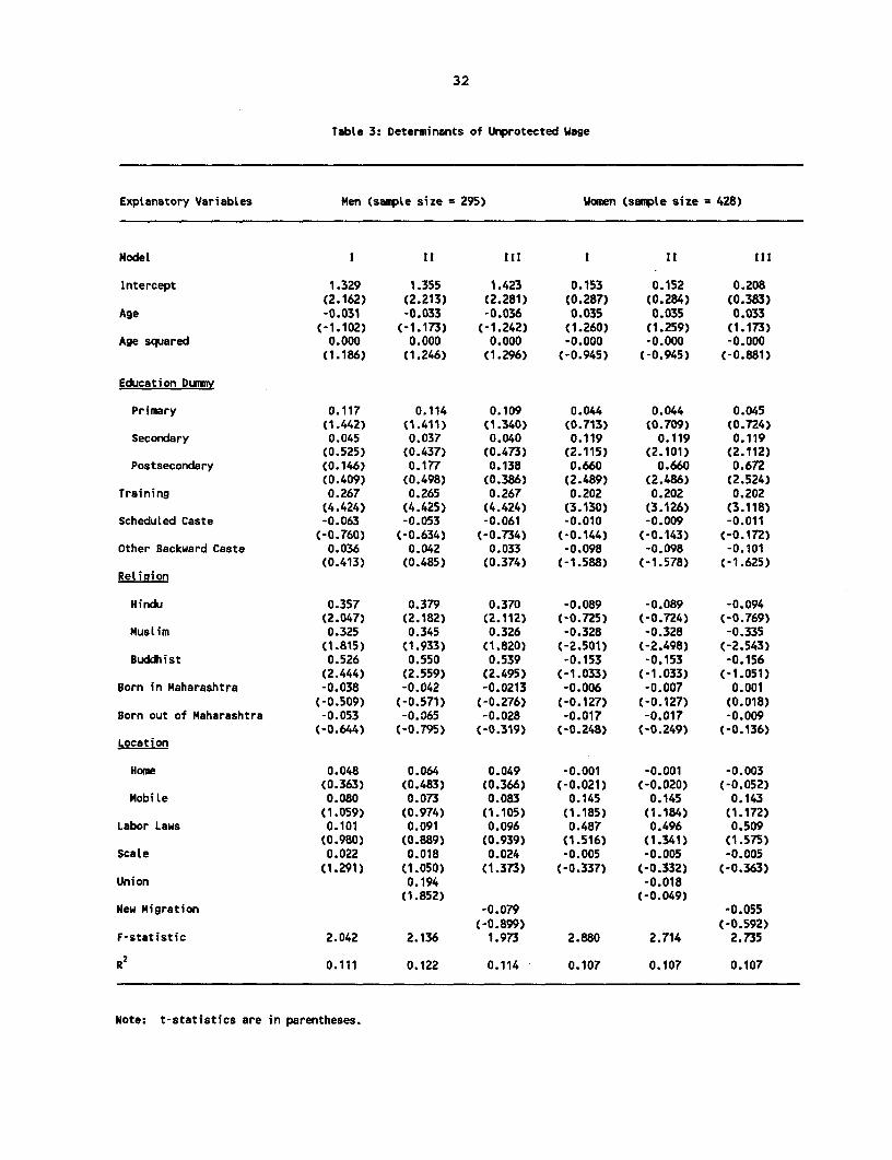
32

TabLe 3: Determinants of Unprotected Wage

Explanatory VariabLes Men (sampLe size = 295) Women (sample size = 428)

ModeL I II 1ll 1 11 II

Intercept 1.329 1.355 1.423 0.153 0.152 0.208(2.162) (2.213) (2.281) (0.287) (0.284) (0.383)

Age -0.031 -0.033 -0.036 0.035 0.035 0.033(-1.102) (-1.173) (-1.242) (1.260) (1.259) (1.173)

Age squared 0.000 0.000 0.000 -0.000 -0.000 -0.000(1.186) (1.246) (1.296) (-0.945) (-0.945) (-0.881)

Education Dummy

Primary 0.117 0.114 0.109 0.044 0.044 0.045(1.442) (1.411) (1.340) (0.713) (0.709) (0.724)

Secondary 0.045 0.037 0.040 0.119 0.119 0.119(0.525) (0.437) (0.473) (2.115) (2.101) (2.112)

Postsecondary (0.146) 0.177 0.138 0.660 0.660 0.672(0.409) (0.498) (0.386) (2.489) (2.486) (2.524)

Training 0.267 0.265 0.267 0.202 0.202 0.202(4.424) (4.425) (4.424) (3.130) (3.126) (3.118)

Scheduled Caste -0.063 -0.053 -0.061 -0.010 -0.009 -0.011(-0.760) (-0.634) (-0.734) (-0.144) (-0.143) (-0.172)

Other Backward Caste 0.036 0.042 0.033 -0.098 -0.098 -0.101(0.413) (0.485) (0.374) (-1.588) (-1.578) (-1.625)

ReLigion

H:indu 0.357 0.379 0.370 -0.089 -0.089 -0.094(2.047) (2.182) (2.112) (-0.725) (-0.724) (-0.769)

Muslim 0.325 0.345 0.326 -0.328 -0.328 -0.335(1.815) (1.933) (1.820) (-2.501) (-.2.498) (-2.543)

Buddhist 0.526 0.550 0.539 -0.153 -0.153 -0.156(2.444) (2.559) (2.495) (-1.033) (-1.033) (-1.051)

Born in Maharashtra -0.038 -0.042 -0.0213 -0.006 -0.007 0.001(-0.509) (-0.571) (-0.276) (-0.127) (-0.127) (0.018)

Born out of Maharashtra -0.053 -0.065 -0.028 -0.017 -0.017 -0.009(-0.644) (-0.795) (-0.319) (-0.248) (-0.249) (-0.136)

Location

Home 0.048 0.064 0.049 -0.001 -0.001 -0.003(0.363) (0.483) (0.366) (-0.021) (-0.020) (-0.052)

MobiLe 0.080 0.073 0.083 0.145 0.145 0.143(1.059) (0.974) (1.105) (1.185) (1.184) (1.172)

Labor Laws 0.101 0.091 0.096 0.487 0.496 0.509(0.980) (0.889) (0.939) (1.516) (1.341) (1.575)

ScaLe 0.022 0.018 0.024 -0.005 -0.005 -0.005(1.291) (1.050) (1.373) (-0.337) (-0.332) (-0.363)

Union 0.194 -0.018(1.852) (-0.049)

New Migration -0.079 -0.055(-0.899) (-0.592)

F-statistic 2.042 2.136 1.973 2.880 2.714 2.735

R2 0.111 0.122 0.114 0.107 0.107 0.107

Note: t-statistics are in parentheses.

33

Table 4: Determinants of Hourly Earnings from Self-employment

Explanatory Variables Men (sample size 482) Women (sample size = 196)

Model I 11 III I ll III

Intercept 1.487 1.382 1.675 0.419 0.449 0.181(2.547) (2.586) (2.835) (0.401) (0.483) (0.168)

Age -0.005 -0.007 -0.014 0.059 0.039 0.072(-0.175) (-0.295) (-0.516) (1.183) (0.866) (1.377)

Age squared -0.000 0.000 0.000 -0.001 -0.000 -0.000(-0.053) (0.041) (0.255) (-1.215) (-0.885) (-1.396)

Education Dummu

Primary 0.222 0.148 0.219 -0.111 -0.106 -0.129(2.915) (2.104) (2.884) (-0.786) (-0.844) (-0.905)

Secondary 0.307 0.217 0.305 0.069 0.018 0.065(3.977) (3.038) (3.961) (0.581) (0.173) (0.552)

Postsecondary 0.510 0.396 0.509(3.499) (2.960) (3.505)

Training 0.032 0.108 0.035 -0.020 0.216 -0.018(0.602) (2.205) (0.673) (-0.155) (1.811) (-0.138)

Scheduled Caste -0.005 0.010 -0.002 -0.129 -0.150 -0.013(-0.062) (0.127) (-0.020) (-0.916) (-0.120) (-0.919)

Other Backward Caste -0.060 -0.077 -0.057 0.172 0.042 0.174(-0.716) (-1.009) (-0.680) (1.290) (0.351) (1.303)

Religion

Hindu -0.267 -0.179 -0.253 -0.169 -0.025 -0.180(-2.882) (-2.101) (-2.737) (-0.708) (-0.115) (-0.752)

Muslim -0.290 -0.221 -0.289 -0.118 -0.041 -0.113(-3.005) (-2.492) (-3.008) (-0.452) (-0.174) (-0.429)

Buddhist -0.180 -0.110 -0.187 0.032 0.060 0.017(-1.057) (-0.703) (-1.104) (0.111) (0.237) (0.058)

Born in Maharashtra 0.050 0.046 0.071 -0.061 -0.095 -0.083(0.631) (0.634) (0.877) (-0.508) (-0.888) (-0.674)

Born out of Maharashtra 0.105 0.060 0.131 -0.093 -0.097 -0.119(1.367) (0.854) (1.682) (-0.618) (-0.724) (-0.776)

Location

Home -0.050 0.009 -0.043 -0.135 -0.023 -0.141(-0.744) (0.142) (-0.645) (-1.147) (-0.220) (-1.197)

Mobile 0.107 0.151 0.124 0.195 0.198 0.200(1.474) (2.259) (1.696) (1.363) (1.555) (1.396)

Scale 0.183 0.154 0.186 -0.014 -0.025 -0.017(6.995) (6.397) (7.112) (-0.246) (-0.483) (-0.303)

Sales 0.0002 0.001(9.525) (6.936)

New Migration -0.215 0.215(-1.879) (0.895)

F-statistic 7.156 13.372 6.980 0.935 4.113 0.925

R2 0.198 0.329 0.204 0.072 0.269 0.076

Note: t-statistics are in parentheses

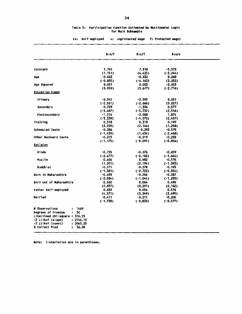
34

Table 5: Participation Function Estimated by Multinomiat Logitfor Mate SubsampLe

(s: Setf-employed c: Unprotected Wage f: Protected wage)

B:s/f B:c/f B:s/c

Constant 1.745 7.318 -5.573(1.151) (4.425) (-3.24)

Age -0.063 -0.332 0.269(-0.855) (-4.163) (3.252)

Age Squared 0.001 0.003 -0.003(0.959) (3.677) (-2.716)

Education Dumw

Primary -0.545 -0.595 0.051(-2.561) (-2.666) (0.227)

Secondary -0.729 -1.306 0.577(-3.487) (-5.732) (2.516)

Postsecondary -1.214 -3.088 1.874(-3.339) (-4.072) (2.407)

Training 0.518 0.319 0.199(3.939) (2.146) (1.258)

ScheduLed Caste -0.286 0.293 -0.579(-1.439) (1.434) (-2.468)

Other Backward Caste -0.223 -0.019 -0.203(-1.175) (-0.091) (-0.856)

ReLigion

Hindu -0.735 -0.076 -0.659(-2.677) (-0.182) (-1.644)

MusLim 0.406 0.982 -0.576(1.301) (2.194) (-1.393)

Buddhist -0.571 -0.378 -0.193(-1.381) (-0.722) (-0.354)

Born in Maharashtra -0.493 -0.206 -0.287(-2.584) (-1.044) (-1.290)

Born out of Maharashtra 0.560 0.064 0.496(2.837) (0.291) (2.162)

Father Self-emptoyed 0.630 0.054 0.576(4.571) (0.349) (3.499)

Married -0.411 -0.211 -0.200(-1.738) (-0.833) (-0.577)

# Observations 1469Degrees of Freedom : 30Likelihood chi-square : 316.55-2 Llikef (slope) : 2746.70-2 Ltikef (const) : 3063.25X Correct Pred : 56.09

Note: t-statistics are in parentheses.

35

Table 6. Participation Function Estimated by Multinomial Logitfor Female Subsample

(s: Self-employed c: Unprotected Wage f: Protected wage)

B:s/f B:c/f B:s/c

Constant 4.309 7.749 -3.440(1.241) (2.416) (-1.653)

Age -0.295 -0.355 0.060(-1.593) (-2.061) (0.570)

Age Squared 0.004 0.004 -0.000(1.709) (1.959) (-0.238)

Education Dummy

Primary -0.351 -0.275 -0.076(-0.879) (-0.775) (-0.288)

Secondary -0.208 -0.635 0.427(-0.636) (-2.142) (1.907)

Training -0.453 -0.809 0.356(-1.424) (-2.879) (1.434)

ScheduLed Caste 0.816 0.538 0.278(1.905) (1.361) (1.043)

Other Backward Caste -0.282 -0.178 -0.104(-0.825) (-0.600) (-0.404)

ReLigion

Hindu 0.269 0.322 -0.053(0.433) (0.590) (-0.110)

Muslim 2.228 2.126 0.102(2.357) (2.398) (0.196)

Buddhist -0.410 -0.179 -0.231(-0.510) (-0.248) (-0.399)

Born in Maharashtra 0.490 0.039 0.451(1.518) (0.138) (1.931)

Born out of Maharashtra 0.663 0.342 0.321(1.478) (0.830) (1.116)

Father Self-employed 0.887 0.383 0.503(3.073) (1.452) (2.607)

Married 0.837 0.700 0.137(2.845) (2.728) (0.352)

# Observations : 723Degrees of Freedom 28Likelihood chi-square 89.12-2 LLikef (slope) : 1265.02-2 Llikef (const) 1354.15% Correct Pred : 59.89

Note: t-statistics are in parentheses.

36

Table 7: Predicted Mate Participation by Sample Characteristics

Setf-employed Unprotected ProtectedWage wage

SchooLing

Less than Primary 0.372 0.319 0.309Primary 0.308 0.251 0.440Secondary 0.312 0.150 0.537Post-secondary 0.255 0.034 0.711

Vocational Training

Yes 0.373 0.201 0.426No 0.138 0.015 0.847

Caste

Scheduled Caste 0.272 0.244 0.483Other Backward Caste 0.305 0.188 0.508Other 0.352 0.177 0.470

Rel iaion

Hindu 0.285 0.186 0.529Muslim 0.456 0.274 0.270Buddhist 0.335 0.137 0.527Other 0.449 0.152 0.399

Birtholace

Bombay 0.240 0.198 0.562Maharashtra State 0.455 0.172 0.373Outside Maharashtra State 0.328 0.203 0.469

Father's Work Status

Self-employed 0.257 0.209 0.534Wage worker 0.390 0.178 0.432

Marital Status

Single 0.318 0.193 0.489Married 0.397 0.198 0.405

Average Predicted Probability 0.325 0.194 0.481Actual Participation 0.328 0.201 0.471

37

Table 8: Predicted Female Participation by Sample Characteristics

Setf-employed Unprotected Wage Protected wage

A B A B A BSchooling

Less than Primary 0.239 0.294 0.683 0.337 0.078 0.368Primary 0.220 0.235 0.678 0.257 0.102 0.508Secondary 0.306 0.236 0.571 0.152 0.123 0.612

Vocational Training

Yes 0.300 0.355 0.524 0.270 0.176 0.376No 0.301 0.223 0.570 0.142 0.129 0.635

Caste

Scheduled Caste 0.274 0.296 0.621 0.252 0.105 0.452Other Backward Caste 0.247 0.268 0.634 0.243 0.119 0.488Other 0.253 0.321 0.623 0.230 0.124 0.449

Religion

Hindu 0.266 0.297 0.604 0.243 0.130 0.460Muslim 0.275 0.413 0.596 0.224 0.129 0.363Buddhist 0.306 0.346 0.546 0.210 0.148 0.444Other 0.264 0.412 0.579 0.210 0.157 0.378

Bi rthplace

Bombay 0.256 0.268 0.627 0.260 0.117 0.473Maharashtra State 0.282 0.401 0.626 0.231 0.092 0.367Outside Maharashtra State 0.216 0.308 0.658 0.261 0.125 0.431

Father's Work Status

Self-employed 0.218 0.230 0.645 0.270 0.136 0.500Wage worker 0.328 0.355 0.587 0.235 0.085 0.411

Marital Status

Single 0.281 0.267 0.628 0.252 0.091 0.481Married 0.232 0.338 0.595 0.260 0.174 0.402

Average Predicted Probability 0.268 0.286 0.623 0.255 0.109 0.459Actual Participation 0.271 0.271 0.592 0.592 0.137 0.137Predicted Probability 0.265 0.551 0.682 0.270 0.053 0.179

Note: Estimates in coLumns A are based on the coefficients of women's participation equation, while estimatesin B use the men's participation coefficients. Asterisk C ) refers to the predicted probabilityestimates based on the participation equation which includes location dummies as additional regressorsin the participation equation.

38

Table 9: Employment Function (Hours Worked) Estimation.

Men Women

Self- Unprotected Protected Self- Unprotected ProtectedEmpLoyed Wage Wage EmpLoyed Wage Wage

Constant 61.794 67.935 72.556 19.210 48.674 73.428(3.348) (2.935) (6.906) (0.781) (3.157) (2.585)

Age 1.071 0.633 0.208 3.863 -0.276 -0.824(1.325) (0.648) (0.392) (2.832) (-0.342) (-0.506)

Age Squared -0.013 -0.008 -0.003 -0.045 0.004 0.012(-1.375) (-0.706) (-0.410) (-2.685) (0.410) (0.564)

Scheduled Caste -4.590 -2.252 1.110 -0.926 3.467 2.451(-1.774) (-0.779) (0.985) (-0.238) (1.802) (0.728)

Other Backward Caste -1.145 -1.634 -0.884 4.034 1.719 3.114(-0.468) (-0.559) (-0.814) (1.074) (0.921) (1.467)

Relicion

Hindu -0.869 -9.726 -4.434 -8.796 1.200 -3.009(-0.288) (-1.587) (-2.084) (-1.494) (0.335) (0.767)

Muslim -1.420 -9.678 -5.516 -7.696 1.629 -3.653(-0.457) (-1.551) (-2.129) (-1.237) (0.369) (-0.517)

Buddhist -7.012 -9.796 -6.657 -6.423 2.038 -6.546(-1.363) (-1.253) (-2.487) (-1.009) (0.464) (-1.165)

Born in Maharashtra 1.910 -1.352 0.414 0.219 -2.084 -1.164(0.811) (-0.536) (0.391) (0.080) (-1.379) (-0.539)

Born out of Maharashtra 4.893 7.281 0.949 1.820 -4.107 -1.941(2.182) (2.615) (0.748) (0.538) (-2.125) (0.603)

Location

Home -4.868 -5.197 6.841 -7.602 -4.418 -19.939(-2.464) (-1.187) (1.523) (-2.399) (-3.242) (-4.416)

MobiLe -4.215 3.523 -2.775 -0.899 -10.050 -21.979(-1.997) (1.460) (-1.059) (-0.213) (-2.874) (-2.451)

Wage Predicted -11.506 -10.203 -10.899 -30.505 1.886 -8.590(-3.338) (-1.540) (-5.812) (-1.995) (0.312) (-2.796)

No. of Observations 482.00 295.00 692.00 196.00 428.00 99.00

R2 0.082 0.106 0.090 0.108 0.072 0.321

F-Statistic 3.482 2.779 5.607 1.844 2.675 3.392

Degrees of Freedom 469.00 282.00 679.00 183.00 415.00 86.00

Note: t-statistics are in parentheses.

39

Table 10: Censored Regression (Tobit) Estimates of Occupational Mobility

Exoaenous Variable Parameter Estimate

Male Female

Intercept 0.584 (0.607) 0.118 (0.0830)

Age 0.025 (0.536) 0.215 (0.293)

Age squared -0.0001 (-0.023) -0.000 0-0.045)

Education Dumm

Primary 0.414 (3.096) 0.209 (1.156)

Secondary 0.269 (2.041) 0.347 (2.255)

Postsecondary 0.132 (0.557) 0.134 (0.180)

Training 0.143 (1.693) 0.095 (0.575)

Scheduled Caste -0.198 (-1.595) -0.005 (-0.026)

Other Backward Caste 0.057 (0.463) 0.128 (0.763)

Religion

Hindu 0.020 (0.108) -0.514 (-1.617)

Muslim 0.239 (1.173) -0.423 (-1.203)

Buddhist 0.302 (1.136) -0.476 (-1.218)

Born in Maharashtra -0.179 (-1.490) -0.085 (-0.559)

Born out of Maharashtra -0.388 (-3.009) -0.946 (-4.612)

Father Self-emptoyed -0.330 (-3.758) -0.058 (-0.439)

Married 0.003 (0.022) -0.0003 (-0.002)

Log-likelihood -2251.6 -958.7

Sample Size 1469 723

Note: t-statistics are in parentheses.

40

Table 11: MNL Estimates of the Determinants of Occupational Nobility amongThe Unprotected Wage Workers

Explanatory Variables Men Women

s/c f/c s/f s/c f/c s/f

Intercept -3.058 -2.780 0.280 -23.052 -9.622 -13.430(-1.130) (-1.130) (0.112) (-0.012) (-1.350) (-0.700)

Age 0.207 0.300 -0.893 0.131 0.582 -0.450(2.016) (3.090) (-0.911) (0.816) (1.974) (-1.390)

Age squared -0.180 -0.300 0.121 -0.103 -0.732 -0.630(-1.484) (-2.630) (1.040) (-0.523) (-1.874) (1.480)

Education Dummv

Primary 0.400 1.180 -0.783 0.305 0.480 -0.170(1.202) (3.840) (-2.370) (0.664) (0.820) (-0.242)

Secondary 0.940 1.430 -0.500 0.960 0.590 -0.370(3.180) (5.160) (-1.702) (2.231) (0.923) (-0.504)

Postsecondary 1.880 3.270 -1.390(1.660) (3.080) (-2.424)

Training 0.190 -0.380 0.570 -0.682 0.861 -0.793(0.950) (-2.130) (3.170) (0.174) (2.200) (-1.554)

Scheduled Caste -0.853 -0.460 -0.808 0.900 -0.829 0.740(-2.630) (-0.180) (-2.730) (-0.205) (-1.352) (1.030)

Other Backward Caste -0.400 0.304 -0.702 -0.381 0.463 -0.501(-1.230) (1.120) (-2.493) (0.100) (1.050) (-0.903)

Religio

Hindu -1.230 -0.360 -0.864 15.620 -0.480 15.140(-2.120) (-0.601) (-2.270) (0.008) (-0.350) (0.790)

Muslim -1.050 -0.760 0.290 15.440 -0.480 15.920(-1.670) (-1.160) (0.630) (0.008) (-0.200) (0.830)

Buddhist -0.340 -0.450 -0.790 16.154 0.860 15.293(-0.440) (-0.610) (-1.344) (0.008) (0.572) (0.008)

Born in Maharashtra -0.310 -0.760 -0.235 0.341 -0.612 0.953(-1.090) (-0.320) (-0.914) (0.591) (-0.740) (1.001)

Born out of Maharashtra 0.210 -0.630 0.840 0.330 -0.880 1.204(0.690) (-2.207) (2.944) (0.571) (-1.080) (1.282)

Father Self-employed 0.230 -0.580 0.808 0.380 -0.330 0.706(0.830) (-2.280) (3.150) (1.130) (-0.470) (1.350)

Married -0.203 0.320 -0.522 -0.150 -0.570 0.421(-0.610) (1.020) (-1.600) (-0.461) (-1.501) (0.920)

Predicted ProbabiLity of -1.990 -6.005 4.013 2.250 5.50 7.750being initially in (-0.840) (-2.790) (1.841) (0.430) (0.706) (0.880)unprotected wage work

Maximum Likelihood -847.90 -303.63

Sample size 894 494

Note: t-statistics are in parentheses.

s/c-refers to the probability of switching to self-employment compared to remaining in the unprotectedwage work;

f/c-refers to the probability of switching to protected wage work compared to staying in the unprotectedwage sector;

s/f-measures the probabiLity of switching to self-employment relative to switching to protected wageemployment.

41

Table 12: Random Effects Estimates of Income Mobility

Exogenous Variable Parameter Estimate

Male Female

Intercept 481.571 (9.488) 278.320 (10.204)

Year -198.308 (-14.560) -119.940 (-13.467)

Age 1.863 (1.822) -1.337 (-1.369)

Age squared 0.0004 (0.016) 0.030 (2.019)

Education Dummv

Primary 34.805 (4.052) -1.939 (-0.286)

Secondary 56.906 (6.719) 12.560 (2.243)

Postsecondary 113.031 (7.265) 63.001 (2.223)

Training -2.577 (-0.436) 18.389 (2.594)

Scheduled Caste -11.284 (-1.406) 3.883 (0.545)

Other Backward Caste -14.746 (-1.876) 6.172 (0.959)

Religion

Hindu -52.738 (-4.332) -10.025 (-0.819)

Muslim -58.708 (-4.432) -28.318 (-2.096)

Buddhist -44.763 (-2.592) -6.110 (-0.407)

Born in Maharashtra 0.421 (0.055) -6.320 (-1.076)

Born out of Maharashtra 4.138 (0.505) -7.855 (-1.056)

Father Self-employed -2.577 (-0.436) 6.321 (1.227)

F-Statistics 589.501 154.385

Sample Size 1469 723

Hausman SpecificationTest (Chi-square, 3) 12.8 2.97

Note: t-statistics are in parentheses.

Appedix

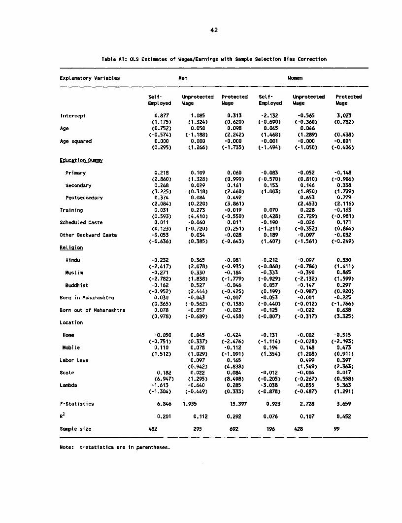
42

TabLe Al: OLS Estimates of Wages/Earnings with Sample SeLection Bias Correction

ExpLanatory Variables Men Women

SeLf- Unprotected Protected Self- Unprotected ProtectedEmployed Wage Wage EmpLoyed Wage Wage

Intercept 0.877 1.085 0.313 -2.132 -0.565 3.023(1.175) (1.324) (0.620) (-0.690) (-0.360) (0.782)

Age (0.752) 0.050 0.098 0.045 0.046(-0.574) (-1.188) (2.242) (1.468) (1.289) (0.438)

Age squared 0.000 0.000 -0.000 -0.001 -0.000 -0.001(0.295) (1.266) (-1.735) (-1.494) (-1.050) (-0.406)

Education Dummy

Primary 0.218 0.109 0.060 -0.083 -0.052 -0.148(2.860) (1.328) (0.999) (-0.570) (0.810) (-0.906)

Secondary 0.268 0.029 0.161 0.153 0.146 0.338(3.225) (0.318) (2.460) (1.003) (1.850) (1.729)

Postsecondary 0.374 0.084 0.492 0.653 0.779(2.084) (0.220) (3.861) (2.453) (2.116)

Training 0.031 0.273 -0.019 0.070 0.228 -0.163(0.593) (4.410) (-0.550) (0.428) (2.729) (-0.981)

Scheduled Caste 0.011 -0.060 0.011 -0.190 -0.026 0.171(0.123) (-0.720) (0.251) (-1.211) (-0.352) (0.864)

Other Backward Caste -0.053 0.034 -0.028 0.189 -0.097 -0.032(-0.636) (0.385) (-0.643) (1.407) (-1.561) (-0.249)

Religion

Hindu -0.232 0.365 -0.081 -0.212 -0.097 0.330(-2.417) (2.078) (-0.935) (-0.868) (-0.786) (1.411)

MusLim -0.271 0.330 -0.184 -0.333 -0.390 0.865(-2.782) (1.838) (-1.779) (-0.929) (-2.132) (1.599)

Buddhist -0.162 0.527 -0.046 0.057 -0.147 0.297(-0.952) (2.444) (-0.425) (0.199) (-0.987) (0.920)

Born in Maharashtra 0.030 -0.043 -0.007 -0.053 -0.001 -0.225(0.365) (-0.562) (-0.158) (-0.440) (-0.012) (-1.766)

Born out of Maharashtra 0.078 -0.057 -0.023 -0.125 -0.022 0.638(0.978) (-0.689) (-0.458) (-0.807) (-0.317) (3.325)

Location

Home -0.050 0.045 -0.424 -0.131 -0.002 -0.515(-0.751) (0.337) (-2.476) (-1.114) (-0.028) (-2.193)

MobiLe 0.110 0.078 -0.112 0.194 0.148 0.473(1.512) (1.029) (-1.091) (1.354) (1.208) (0.911)

Labor Laws 0.097 0.165 0.499 0.397(0.942) (4.838) (1.549) (2.363)

ScaLe 0.182 0.022 0.084 -0.012 -0.004 0.017(6.947) (1.295) (8.498) (-0.205) (-0.267) (0.558)

Lambda -1.613 -0.640 0.285 -3.038 -0.855 5.363(-1.304) (-0.449) (0.333) (-0.878) (-0.487) (1.291)

F-Statistics 6.846 1.935 15.397 0.923 2.728 3.659

R2 0.201 0.112 0.292 0.076 0.107 0.452

SampLe size 482 295 692 196 428 99

Note: t-statistics are in parentheses.

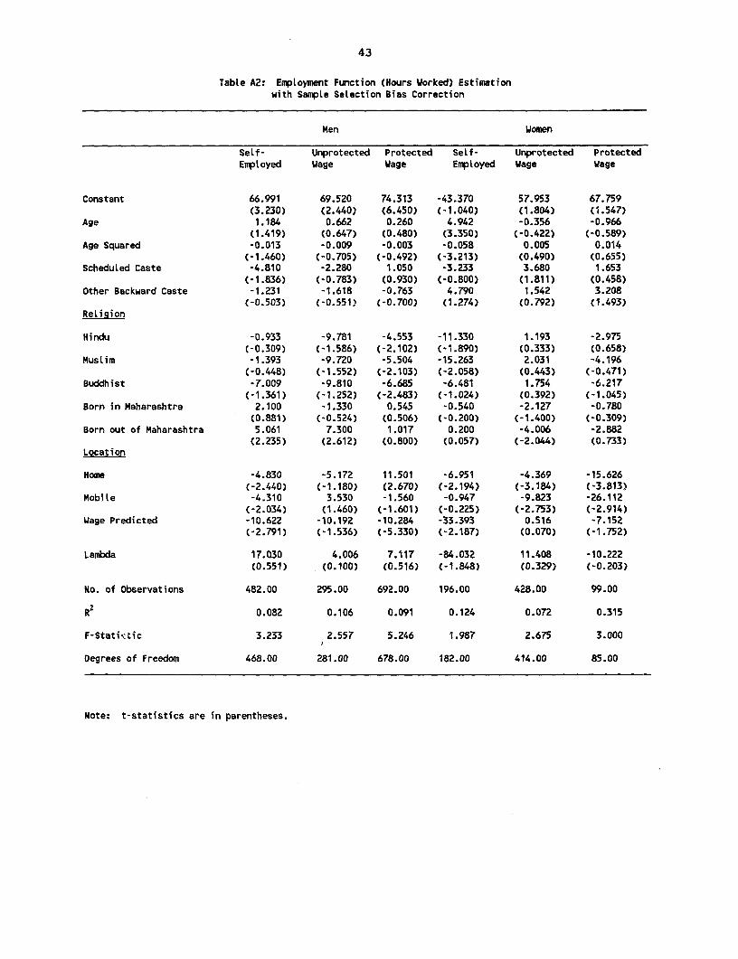
43

Table A2: Employment Function (Hours Worked) Estimationwith SampLe SeLection Bias Correction

Men Women

SeLf- Unprotected Protected Self- Unprotected ProtectedEmployed Wage Wage Employed Wage Wage

Constant 66.991 69.520 74.313 -43.370 57.953 67.759(3.230) (2.440) (6.450) (-1.040) (1.804) (1.547)

Age 1.184 0.662 0.260 4.942 -0.356 -0.966(1.419) (0.647) (0.480) (3.350) (-0.422) (-0.589)

Age Squared -0.013 -0.009 -0.003 -0.058 0.005 0.014(-1.460) (-0.705) (-0.492) (-3.213) (0.490) (0.655)

Scheduled Caste -4.810 -2.280 1.050 -3.233 3.680 1.653(-1.836) (-0.783) (0.930) (-0.800) (1.811) (0.458)

Other Backward Caste -1.231 -1.618 -0.763 4.790 1.542 3.208(-0.503) (-0.551) (-0.700) (1.274) (0.792) (1.493)

Religion

Hindu -0.933 -9.781 -4.553 -11.330 1.193 -2.975(-0.309) (-1.586) (-2.102) (-1.890) (0.333) (0.658)

Muslim -1.393 -9.720 -5.504 -15.263 2.031 -4.196(-0.448) (-1.552) (-2.103) (-2.058) (0.443) (-0.471)

Buddhist -7.009 -9.810 -6.685 -6.481 1.754 -6.217(-1.361) (-1.252) (-2.483) (-1.024) (0.392) (-1.045)

Born in Maharashtra 2.100 -1.330 0.545 -0.540 -2.127 -0.780(0.881) (-0.524) (0.506) (-0.200) (-1.400) (-0.309)

Born out of Maharashtra 5.061 7.300 1.017 0.200 -4.006 -2.882(2.235) (2.612) (0.800) (0.057) (-2.044) (0.733)

Location

Home -4.830 -5.172 11.501 -6.951 -4.369 -15.626(-2.440) (-1.180) (2.670) (-2.194) (-3.184) (-3.813)

Mobile -4.310 3.530 -1.560 -0.947 -9.823 -26.112(-2.034) (1.460) (-1.601) (-0.225) (-2.753) (-2.914)

Wage Predicted -10.622 -10.192 -10.284 -33.393 0.516 -7.152(-2.791) (-1.536) (-5.330) (-2.187) (0.070) (-1.752)

Lambda 17.030 4.006 7.117 -84.032 11.408 -10.222(0.551) (0.100) (0.516) (-1.848) (0.329) (-0.203)

No. of Observations 482.00 295.00 692.00 196.00 428.00 99.00

R2 0.082 0.106 0.091 0.124 0.072 0.315

F-StatitUtic 3.233 2.557 5.246 1.987 2.675 3.000

Degrees of Freedom 468.00 281.00 678.00 182.00 414.00 85.00

Note: t-statistics are in parentheses.

44

Table A3: Probit Estimates of the Determinants of Occupational Mobility amongthe SeLf-employed

Explanatory Variables Men Women

f/s c/s f/c c/s

Intercept -7.509 -0.173 -16.677 -6.575(-1.760) (0.000) (-0.018) (-1.517)

Age 0.150 -0.331 1.482 0.087(0.752) (-1.493) (1.451) (0.401)

Age squared -0.002 0.004 -0.015 -0.001(-0.680) (1.325) (-1.267) (-0.446)

Education Dummv

Primary 1.406 0.011 -3.289 0.981(1.829) (0.018) (-1.126) (1.862)

Secondary 1.606 0.203 -1.203 -0.321(2.006-) (0.311) (-0.502) (-0.827)

Postsecondary 1.608 -5.998 10.209(2.339) (-0.008) (0.015)

Training 0.279 0.180 -0.259 -0.126(0.943) (0.561) (-0.272) (-0.293)

Scheduled Caste -0.311 -0.007 0.620 -1.865(-0.700) (-0.016) (0.558) (-2.842)

Other Backward Caste 0.239 0.446 -3.328 0.665(0.470) (0.845) (-1.755) (0.875)

Reliaion

Hindu 0.549 6.149 -6.576 2.494(1.026) (0.011) (-0.007) (2.241)

Muslim -0.943 6.091 -5.613 -1.874(-1.526) (0.011) (-0.006) (-0.005)

Buddhist 2.396 0.824 -3.040 5.072(2.287) (0.001) (0.003) (2.886)

Born in Maharashtra 1.039 -1.147 1.268 -2.935(1.824) (-2.043) (1.188) (-2.709)

Born out of Maharashtra -0.108 -1.325 3.468 -2.840(-0.199) (-2.633) (1.596) (-2.368)

Father Self-employed -2.144 -1.102 -0.777 -2.407(-4.159) (-2.061) (-0.731) (-2.465)

Married 0.877 0.357 -2.780 -0.579(1.632) (0.649) (-1.993) (-1.469)

Predicted probability 9.618 6.652 -43.993 23.836of being initially (1.625) (1.114) (-1.570) (2.313)self-employed

Log-Likelihood -57.582 -41.241 -11.383 -45.719

Sample size 182 170 50 149

Note: t-statistics are in parentheses.

f/s-measures the probability of switching to protected wage relativeto remaining self-employed;

c/s-measures the probabiLity of switching to unprotected wage reLativeto remaining self-employed;

f/c-measures the probability of switching to protected wage relativeto switching to unprotected wage.

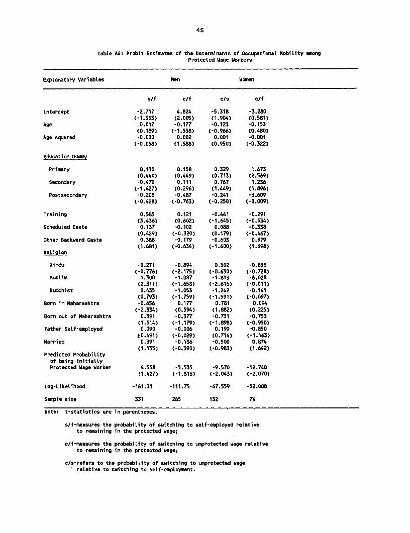
45

Table A4: Probit Estimates of the Determinants of Occupational Mobility amongProtected Wage Workers

Explanatory Variables Men Women

s/f c/f c/s c/f

Intercept -2.717 4.824 -5.318 -3.280(-1.353) (2.005) (1.904) (0.581)

Age 0.017 -0.177 -0.123 -0.153(0.189) (-1.558) (-0.966) (0.480)

Age squared -0.000 0.002 0.001 -0.001(-0.058) (1.588) (0.950) (-0.322)

Education Dummw

Primary 0.130 0.158 0.329 1.673(0.440) (0.449) (0.713) (2.569)

Secondary -0.470 0.111 0.767 1.236(-1.427) (0.296) (1.449) (1.896)

Postsecondary -0.208 -0.487 -0.241 -3.609(-0.428) (-0.763) (-0.250) (-0.009)

Training 0.585 0.121 -0.441 -0.291(3.436) (0.602) (-1.645) (-0.534)

Scheduled Caste 0.137 -0.102 0.088 -0.338(0.429) (-0.320) (0.179) (-0.467)

Other Backward Caste 0.388 -0.179 -0.603 0.979(1.681) (-0.634) (-1.600) (1.698)

Religion

Hindu -0.271 -0.894 -0.302 -0.858(-0.776) (-2.175) (-0.630) (-0.728)

Muslim 1.300 -1.087 -1.813 -6.028(2.311) (-1.658) (-2.616) (-0.011)

Buddhist 0.435 -1.053 -1.242 -0.141(0.793) (-1.759) (-1.591) (-0.097)

Born in Maharashtra -0.656 0.177 0.781 0.094(-2.334) (0.594) (1.882) (0.225)

Born out of Maharashtra 0.391 -0.377 -0.731 -0.753(1.514) (-1.179) (-1.898) (-0.950)

Father Self-employed 0.090 -0.006 0.199 -0.850t0.491) (-0.029) (0.714) (-1.163)

Married 0.391 -0.136 -0.500 0.874(1.135) (-0.390) (-0.983) (1.642)

Predicted Probabilityof being initiallyProtected Wage Worker 4.558 -5.535 -9.570 -12.748

(1.427) (-1.816) (-2.043) (-2.070)

Log-Likelihood -161.31 -111.75 -67.559 -32.088

Sample size 331 285 132 76

Note: t-statistics are in parentheses.

s/f-measures the probability of switching to self-employed relativeto remaining in the protected wage;

c/f-measures the probabitity of switching to unprotected wage relativeto remaining in the protected wage;

c/s-refers to the probability of switching to unprotected wagerelative to switching to self-employment.

Distributors of World Bank PublicationsARtCGNTINA FINtlAD 4LxtcC SOVFtH AFRICA. BOTSWANAC.ds. had SIAL A K*kmqt INFCTEC Fa.oegla IwC_IUCou_, P 1O Bl25 Apdo P 220 22Oded Ulewnty PFlw.A 165. 4d lRmw,Ok 453/465 SF401Ot 14060T[lpnuMd A S..iha AhM.13. 9BooeA HddntI 30 P.O. Q 1141

MOROCCO CapeTo-n vmAUSTILAlA, *PAUA NEW GUINEA. FtWIC SW 'Ehid`E h kMe MuwmFl5L SOLOMON ISLANDS Wwd Batl Pubhiouw, 12rueMmw%d dA.'Ads Fr_ fW.V4ada:VANUATU, AND WESTlEN SAMOA 46.. &nu d'li& CCaM . Iieaonu atit Sulbopboo SlvtOK Book. Ajowual. 751160Pu P.O. DM 41095648 WWidom Rood NETHERLANDS Cr,altMi6dw 3132 GERYAANY hbiOtPubltik} b.v. IJdta_. 2D24Vkld UNO.Vig P.O. Bo 14

Pe.pdarf AbwU5 7ntD SRLAdtc SPAINAUSTRIA D.536 BSut I Mu di-P,o Lbto SACedd I,d CA NEW ZEALAND Cmodlo37CI;nv, 31 GREECE H1 tibty d WoAnSa-c 1w. 301 MadrdA-1011 Wkn KELUE Pniae Bag

24L Ipodaou Steet Plta Faitr Nee Mar,k Ubredt blaraboAI AEDO6EAHEAIN Atlhvr-l45 Audo C-ello deCot 391BSarmn Kd nd VW altacY 0e9w Bardoa

Ag-dao Lld. GUATEMALA NICERIAP.o. Boo 2750 l nbr Pied,i Sata U,dv-ty Pvr, Umited SRI LANKA AND THE MALDIVESMatea To,n 317 11 CaS 6SD Th,e C Buldidg&Jeidho Lake Hn_m BOoI.hop

ZoosI Pnsee Mal 4i SaS0 P.O Bov 24BANGLADESH Cuaalwa CUiy Ii adt 1.4OtampalamA.Mi. Intdb_ Dedopmnt Cdit MatU.

A_ae So"MSI HONG KONG MACAO NORWAY Cddomb*2H.t. 5. Roo 16 AAu RD Lad. Naeren, bmaono CoobwI3aoottd R/A_ 44WyrcnS 5lilartenertt SWEDEN13.. 129 Watla Cite PO Boo 9125 EtteSd Ftogit dle:

2nd Floor NK062 Ola 6 Friti F.&boItortagetB,ooa.ffim Cetnal H-Sn Kor Rqi ntAt 12, B- 13S6Man RIod OMAN S-30327 iSthdl'M-jdeo Ci-t DINA MEMU.R 1oftertaito SebNoa&hab - 3COC Ald Pubbibee Pabe LAd. P.O. Bo 161 alSeeli Akp..t FwMiamiitmada

731 Momt Rod Mn-at WWebrW &aia AB7MXKDAAvenue Mdr.0WOi1 Bev3O04Roles PAKISTAN NS104 25SIOdaih

B8dk of= Mhnu Bo AgeoyBELCIUM 15JN. Herdi Mwg 65. Sid.hnli.e.d-A2a SWrTZERLANDlo De Lowoy Ballard Ease PGOBo -No 729 FaesiirwA, dut Bd Bnmba y-4030i La%oee3 Ulbkte Pa1060 BStmels 4mim CeGm

13/14AolAli BDad PMU Camepoule 3lCANADA Net Dwh - 1106O2 hdiea Demrllb SA CH 1211 GCea ItIa Dlfthwa Aprt 32C.P. 5. IRIBtaepkme 1 Chitnn. Ae limt F cBeud,weitle. Qdwe CAlai. -70D 072 liie PbayJ4B i E6 IHnzr SevkedesnAboone

layhdevadHosed Bulidbeg biawa B. Cee- C patae33i1CHINA 5 Maie Rod Gandhbhar Fihh Row. pbca. Lile Buildbag CHM 102 LaooCltUm PA-d & oeuk B9gloe - 560 m9 Ayala Aat.u Meak

Pbh"* HoAs MetoMiuttl TANZANIAi Da Fb Si D.jie 3-5.1129 Xaciaclta C. Road Okwid uveLty Pt..Bdelft Hydebad,- 503=27 POLAND P.O. Boo 399

ORPAN Dwes SSal.aCOLtOUSIA PFrals fla, 2nd Flo P.c Yito tMbr'anmice LAd. N-wThalke Baug, Nwr.epura O3-41 Waream THAILANDApwtad Aerm 34270 Abomdbd .3100W1 Ceat"l DO. t 9BSoa DA. PORTUGAL 3265.1wc Road

PAWS HI-oom U n.wl PatupI BankDkCOTES DIVOIRB 16-AAaokMas Rua DoCme70.74Cnt,wd'Ed1Ibwtd.DW.6= Ltxo -26(01 172wCl TRNDAD &TOSAGO. ANTIGUA

Aicade (CEIA) BARlUDA, SARBADOS.04 BP. 541 INDONESIA SAUDIARAIA.QATAR DOMNCA. GRENADA, CUYANA.AbidjO 04Plaet Pt Indfrs Llmhed jarlBomkSbe JAMAICA. MONTSERLAT, ST.

it. SW R5 0o 37 P.O. Boo 19 KTTMS NEVIS, ST. UCACYPWUS P.O. Boo 1I1 Ryad 11471 ST. VINCENT GRENADINESMDEMR 1hdartrd. Ser,c. jekw Pu. SyLJnitmSkudimUtP.O. Boa IMS MEtR Wwonio Se-ims *9WiseSIueNlned. ITALY Bnr-ooAg1 CUM"

Lie. Cmamdmi tari Suted SPA Al Alm Stat Trdeda. Wed ldieDEWNAIK Via D.,, Di Ctliba. 120/ 10 Al D1n. Cee-SnA.idolJtr bei CeslC PomeS52 Ft PAMw UNrDT ARAB EMIRATESRo_oeo-AIM II 1252FkPwe P.O. Ba 713 MEMUCulGfCeD0-lED 9 eFrdwebgC AWyN P.O. BS,7

jAPAN 2ODOMINICAN REUULIC ESane Bok Se-wI 1 AHduA Alivta BtdegREte. Te. C pa A. 374 Har4o 34Chme. Bnkyo.ku 113 Kim Kbaled $td UNITD KINGDOMReiawad6e elbot Is Cm6it. 9W Tdoy, P.O. Bo 399 MkaebfoUld.Apat"do Ped 219D D _meses P.O. Bo 3Smie Dbego KENYA Al., Hnompsi CGLU34 7JC

ASic Baok Se-vi (EA) Ld. 31 Yb~ned H-a-b Awed Sh E%eddRCGT. ARAS rusLIC OP P.o Bo 45245 PJD Baw 97SAl Abra Ndtei jeddb VENEZUELAAl G l.. Sota Ulawo de4 EseCAM KORIEA.EWUBLCOF SINGAPOE.TAIWAN, Ap4 od 60337

Pa Kee Book Capaeb MYAN4ASABRUNEI C-o 10-AThe Middl. SEaObS,orw P.O. Boo 101, Ks,&e;hao Wwearbon Publlcabeo41, Slli S. Si Pf., 1Ud. YUGOSLAVIACit 024Y lot Ft, Pei-P. Indurial ).aolowd K

KUWAIT Bld$- P.O. aom 3EL SALVADOR MEMR11Wae-m.Serelo 24 Net htntull Rood TugqesMFu.dw P0 Boo -66S Siegq1963 YU.IlCDBdg.deA.erida Manuel F-6iqeAPaao 03Sa0EdiAdoSlASi I Prim MALAYSIASan Sem,ede- U atvdy od Malaa Coope-sI.

B_x&abyp UeNumdP.O. Boo 1127 Alan Poth BooulRAdl LYD

Recent World Bank Discussion Papers (continued)

No. 126 Agricultural Technology in Sub-Saharan Afiica: A Workshop on Research Issues. Suzanne Gnaegy andJock R.Anderson, editors

No. 127 Using Indigenous Knowledge in Agricultural Development. D. Michael Warren

No. 128 Research on Irrigation and Drainage Technologies: Ffteen Years of World Bank Experience. Raed Safadi andHerve Plusquellec

No. 129 Rent Control in Developing Countries. Stephen Malpezzi and Gwendolyn Bal

No. 130 Patterns of Direct Foreign Investment in China. Zafar Shah Khan

No. 131 A New View of Economic Growth: Four Lectures. Maurice FG. Scott

No. 132 Adjusting Educational Policies: Conserving Resources While Raising School Quality. Bruce Fuller and Aklilu Habte,editors

No. 133 Letting Girls Leam: Promising Approaches in Primary and Secondary Education. Barbara Herz, K. Subbarao,Masooma Habib, and Laura Raney

No. 134 Forest Economics and Policy Analysis: An Overview. William F. Hyde and David H. Newman, with a contributionby Roger A. Sedjo

No. 135 A Strategyfor Fisheries Development. Eduardo Loayza, in collaboration with Lucian M. Sprague

No. 136 Strengthening Public Service Accountability: A Conceptual Framework. Samuel Paul

No. 137 Deferred Cost Recoveryfor Higher Education: Student Loan Programs in Developing Countries. Douglas Albrechtand Adrian Ziderman

No. 138 Coal Pricing in China: Issues and Reforn Strategy. Yves Albouy

No. 139 Portfolio Peformance of Selected Social Security Institutes in Latin America. Carmelo Mesa-Lago

No. 140 Social Security and Prospectsfor Equity in Latin America. Carmelo Mesa-Lago

No. 141 China's Foreign Trade and Comparative Advantage: Prospects, Problems, and Policy Implications. Alexander J. Yeats

No. 142 Restructuring Socialist Industry: Poland's Experience in 1990. Homi J. Kharas

No. 143 China: Industrial Policiesfor an Economy in Transition. Inderjit Singh

No. 144 Reforming Pnrces: The Experience of China, Hungary, and Poland. Anand Rajaram

No. 145 Developing Mongolia. Shahid Yusuf and Shahidjaved Burki

No. 146 Sino-Japanese Economic Relationships: Trade, Direct Investment, and Future Strategy. Shuichi Ono

No. 147 The Effects of Economic Policies on African Agriculture: From Past Harm to Future Hope. William K.Jaeger

No. 148 The Secaoral Foundations of China's Development. Shahidjaved Burki and Shahid Yusuf, editors

No. 149 The Consulting Profession in Developing Countries: A Strategyfor Development. Syed S. Kirmaniand Warren C. Baum

No. 150 Successful Rural Finance Institutions. Jacob Yaron

No. 151 Transport Development in Southern China. Clell G. Harral, editor, and Peter Cook and Edward Holland,principal contributors

No. 152 The Urban Environment and Population Relocation. Michael M. Cemea

No. 153 Funding Mechanismsfor Higher Education: Financingfor Stability, Efficiency, and Responsiveness. Douglas Albrechtand Adrian Ziderman

The World Bank ls

Headquarters European Office Tokyo Office1818 H Street, N.W. 66, avenue d'lena Kokusai Building l_______

Washington, D.C. 20433, U.S.A. 75116 Paris, France 1-1 Marunouchi 3-chomeChiyoda-ku, Tokyo 100, Japan

Telephone: (202) 477-1234 Telephone: (1) 40.69.30.00Facsimnile: (202) 477-6391 Facsimile: (1) 40.69.30.66 Telephone: (3) 3214-5001 uTelex: wULI 64145 wORLDBAN1 Telex: 640651 Facsimile: (3) 3214-3657

RCA 248423 WORLDBK Telex: 26838Cable Address: INT8AFRAD

WASHINGTONDC

0

0

0

0(5as

ISBN 0-8213-2062-9 0-