dynamics of a rigid ship jerzy matusiak - aalto
TRANSCRIPT

NBSI 3-2627-06-259-879 )fdp( L-NSSI 6984-9971
NSSI 6984-9971 )detnirp( NSSI X094-9971 )fdp(
ytisrevinU otlaA
gnireenignE fo loohcS gnireenignE lacinahceM fo tnemtrapeD
if.otlaa.www
+ SSENISUB YMONOCE
+ TRA
+ NGISED ERUTCETIHCRA
+ ECNEICS
YGOLONHCET
REVOSSORC
LAROTCOD SNOITATRESSID
-otl
aA
TS
2/
710
2
kai
suta
M yz
reJ
pih
S di
giR
a fo
sci
many
D y
tisr
evi
nU
otla
A
7102
gnireenignE lacinahceM fo tnemtrapeD
kaisutaM yzreJ
LAIRETAM GNINRAEL + ECNEICS YGOLONHCET
pihS digiR a fo scimanyD

seires noitacilbup ytisrevinU otlaAYGOLONHCET + ECNEICS 2/ 7102
pihS digiR a fo scimanyD
kaisutaM yzreJ
ytisrevinU otlaA gnireenignE fo loohcS
gnireenignE lacinahceM fo tnemtrapeD ygolonhceT eniraM

seires noitacilbup ytisrevinU otlaAYGOLONHCET + ECNEICS 2/ 7102
© kaisutaM yzreJ
NBSI 3-2627-06-259-879 )fdp(
L-NSSI 6984-9971 NSSI 6984-9971 )detnirp( NSSI X094-9971 )fdp(
:NBSI:NRU/if.nru//:ptth 3-2627-06-259-879
noitide detcerroc dnoceS
yO aifarginU iknisleH 7102
dnalniF

Preface
This textbook is a result of the work started in 1996 when I joined a very
interesting, newly formed Specialist Committee working on Ship Stability
within the International Towing Tank Conference (ITTC). Thanks to this
group of international enthusiastic scholars in the field, it became clear for
me that both the research and the rules’ development in the field of ship
stability will proceed in the direction of including ship dynamics into
account. Moreover, this development will require sophisticated
mathematical models of ship dynamics based on the first principles and
taking realistically into account the environmental, often very hostile,
conditions. These models should be verified and thoroughly validated.
I am very grateful to Professor Eero-Matti Salonen for his valuable
comments and corrections he has made to the original manuscript. I want to
thank my colleagues Messrs Teemu Manderbacka and Otto Puolakka, the
assistants in the course on ship dynamics, for their valuable remarks
concerning the lecture notes that were the bases of this report.
I also want to thank Dr. Timo Kukkanen for reviewing the manuscript.

2

3
Contents
Preface ............................................................................................................ 1
Contents ......................................................................................................... 3
List of symbols ............................................................................................... 6
1. Introduction .......................................................................................... 11
2. Basic assumptions ................................................................................ 14
3. Co-ordinate systems and kinematics used for describing ship motion
15
4. General form of equations of motion ................................................. 20
4.1 Equations of translational motion ............................................................ 20 4.2 Equations of angular motion .................................................................... 21
5. In-plane motion of a ship – manoeuvring .......................................... 25
5.1 Slow motion approximation for the hydrodynamic forces .................... 26 5.2 Linear model of a ship’s in-plane motion ................................................ 26 5.3 Straight line stability ................................................................................. 29 5.4 Non-linear model of ship maneuvering .................................................... 33 5.5 Non-dimensional form of the maneuvering equations ........................... 34 5.6 Determination of the slow motion hydrodynamic derivatives ............... 35 5.7 Ship resistance and propeller thrust ........................................................ 37 5.8 Rudder action ............................................................................................. 40 5.9 Azimuth thruster as the main propulsor ................................................. 45 5.10 Autopilot steering .................................................................................... 48 5.11 Aerodynamic forces acting on a ship ..................................................... 48 5.12 Numerical implementation of the maneuvering simulation ................ 50
6. Sea surface waves ................................................................................. 54
6.1 Plane progressive linear regular waves ................................................... 54 6.2 The effects of shallow water ...................................................................... 64

4
6.3 Nonlinear models of surface waves .......................................................... 65 6.4 Wave group ................................................................................................ 68 6.5 Spectral representations of sea surface waves ........................................ 69
7. Hydrodynamic forces acting on a rigid body in waves ..................... 77
7.1 Velocity potential due to ship oscillatory motion and caused by wave
action .................................................................................................................. 77 7.2 Boundary conditions .................................................................................. 79 7.3 Linear hydrodynamic forces in general ................................................... 81 7.4 Hydrostatic forces ...................................................................................... 82 7.5 Nonlinear hydrostatic and Froude-Krylov forces .................................. 85 7.6 Radiation forces ......................................................................................... 87 7.7 Diffraction forces ....................................................................................... 90
8. Single degree of freedom linear system .............................................. 92
8.1 Outline of the solution method ................................................................. 94
9. Linear approximation to ship motion in waves ................................. 98
9.1 Solution to the hydrodynamic problem of ship motions in waves ......... 99 9.2 Outline of the solution of the linear ship motion in waves problem ... 101 9.3 Transfer function of ship motion, response spectra ............................. 102
10. Nonlinear model of ship motion in waves ...................................... 107
10.1 Direct evaluation of ship responses in time domain used in the
program LaiDyn .............................................................................................. 108 10.2 Linear approximation to ship motions in irregular long-crested waves
112 10.3 More on the numerical solution ........................................................... 112 10.4 Two-stage approach .............................................................................. 113
11. Some applications of the theory ...................................................... 115
11.1 Capsizing of a ship in steep regular waves .......................................... 115 11.2 Parametric rolling in regular waves .................................................... 117 11.3 Time-domain simulation of the weather criterion .............................. 120 11.4 The occurrence of roll resonance in stern quartering seas ................ 122
12. Internal loads acting on a rigid hull girder ................................... 129
12.1 Linear approach .................................................................................... 130 12.2 Example ship and linear load evaluation ............................................ 132 12.3 The effect of nonlinearities on internal loads ...................................... 135

5
References .................................................................................................. 140
Appendix A. Co-ordinate systems used in the context of the linear
seakeeping theory .................................................................................... 144
Appendix B Cosine transform using FFT ......................................... 148

6
List of symbols
A amplitude, area
Ap propeller plane area
a added mass coefficient, coefficient
b added damping coefficient
CB volumetric block coefficient
CD drag coefficient
CL lift coefficient
CT total resistance coefficient
CB thrust loading coefficient
D propeller diameter, drag
E energy
F force vector
f function
g constant of gravitational acceleration
G centre of gravity
G moment of external forces

7
h angular momentum
h water depth
H transfer function
HS significant wave height
I matrix comprising components of mass moment of
inertia of the body
I,J,K unit vectors of the Earth-fixed co-ordinate system
i, j,k unit vectors of the body-fixed co-ordinate system
k wave number, retardation function
K coefficient
J advance number
K,M,N components of the moment of external forces
L ship length, lift
M Bending moment
m ship mass, spectral moment
n propeller revolutions per second
n vector normal to the body surface and pointing outwards
of the fluid domain
p,q,r angular velocities in the body-fixed co-ordinate system
p pressure

8
P power
q load distribution
Q shear force
r radius
R position vector
R resistance
S wetted surface, spectral density
t time, thrust deduction factor
T draft, thrust, period
T transformation matrix
U ship velocity vector
u,v,w translational velocities in the body-fixed co-ordinate
system,
flow velocity components in x-, y- and z-directions
V ship speed
v flow velocity vector
w wake factor
x, y, z co-ordinates of the body-fixed co-ordinate system
X,Y,Z co-ordinates of the inertial co-ordinate system

9
components of the hydrodynamic forces acting on ship
hull in the body fixed co-ordinate system
Z number of propellers
α angle of attack
∇ volumetric displacement
β drift angle
γ flow angle, Euler angle
δ rudder angle
ε air-flow angle, phase
θ pitch
λ characteristic value, wave length
μ ship course in respect to waves, heading angle
ρ water density
ρa air density
φ roll, velocity potential
ψ yaw
ω angular velocity
ΩΩ angular velocity vector
ξ critical damping ratio
10
ξj motion component in the j-th degree of freedom
ζ wave elevation

11
1. Introduction
The term ship dynamics means all operational conditions of a vessel where
inertia forces of a ship motion play a role. All situations that differ from the
ideal still water condition with a ship at constant heading and constant
forward speed fall into the category of ship dynamics. Traditionally ship
dynamics is dealt with using different simplified mathematical sub-models
termed sea-keeping, manoeuvring, structural vibration and dynamic
stability. The term directional stability and control is sometimes used
meaning a subclass of the manoeuvring. These sub-models are characterized
by different assumptions. Usually these assumptions concern the linearity of
the responses with respect to the excitation. Thanks to these assumptions it
is possible, using relatively simple algorithms, to predict certain limited
classes of a ship’s behaviour. The shortcoming of these sub-models is that
they are not capable to cope with a wide range of vessel’s behaviour
pertinent to ship safety.
A linear model of ship dynamics in waves called sea-keeping is well
established. In most cases, this model gives a sufficiently accurate
prediction of loads and ship motions. Perhaps the biggest benefit of using a
linear model is that prediction of exceeding a certain level of load or
response can be easily derived. Analysis is conveniently conducted in the
frequency domain. The most serious shortcoming of the linearity
assumption is that it precludes prediction of certain classes of ship
responses. The linear models cannot predict the loss of ship stability in
waves, parametric resonance of roll, and asymmetry of sagging and
hogging. Ship steering and manoeuvring motion are disregarded.
Simulation of ship manoeuvring is usually conducted for the still water
condition. Time-domain simulation of ship motion is restricted to in-plane

12
motion comprising of surge, yaw and sway motion components only. This
means that heeling motion, which is a crucial motion component when ship
safety is concerned, is disregarded. If waves are encountered, their effect is
taken into account as a steady state one.
The main reason for making simplifications in the ship dynamics models
was the poor performance of computers at the time the methods were being
developed (1960’s). On the other hand, a lot of theoretical development
done at this time resulted in the analytical models that are still valid and
very much applicable.
This course on ship dynamics attempts to present a unified theory covering
nonlinear seakeeping and manoeuvring. This model is nearly free of the
linearity assumptions and makes it possible to evaluate a ship’s responses in
the time domain. The model can be used as a basis for an advanced ship-
handling simulator. The forthcoming updated rules concerning stability of
an intact vessel will allow for a direct simulation of ship behaviour in waves
as a direct stability assessment. It is believed that the theory presented in the
course covers the requirements of the method to be used in this task.
The lecture notes for this course can also be used as the theoretical manual
of the LaiDyn software. This computer program has a modular structure.
The separate modules represent the forces developed by rudders and
propellers, hydrodynamic reaction due to hull motion, wave and wind
forces. Mathematical models of these forces are based on basic ship
hydrodynamics; they are presented in detail in the lecture notes. The above-
mentioned reaction forces are used as the excitation to the general model of
a rigid body motion in the six-degrees-of-freedom. This general model,
known from the classical mechanics, is recalled at the beginning of the
course. Next a simplified model of ship dynamics, restricted to the in-plane
motion, is presented. This model is known as manoeuvring. This is a
simplification used amongst the others in the ship-handling simulators used
for training deck officers and pilots. The sub-models representing the action
of propellers and rudders are introduced in the context of manoeuvring.
Numerical implementation of the manoeuvring simulation and the
exemplary results are also given.

13
In Chapter 6, a mathematical model of sea surface waves is presented. This
is done both for regular and irregular waves. Nonlinearities associated with
wave motion are discussed.
In Chapter 7, hydrodynamic reaction forces acting on a ship in waves are
discussed. This is done using a classical potential flow model and making an
allowance for the most important nonlinearities to be taken into account in
the simulation.
Chapter 8 presents a simple, one-degree-of-freedom model of a rigid body
motion in waves. This chapter can be understood as an introduction to sea-
keeping theory.
The model in Chapter 8 is expanded to the linear model of ship motions in
the six-degrees-of-freedom (classical sea-keeping theory) in the beginning
of Chapter 9.
This is followed in Chapter 10 by a presentation of the nonlinear time-
domain model utilized in LaiDyn. This can be thought of as a summary of
what was presented earlier as the separate sub-models and a numerical
implementation of the integration routine.
Chapter 11 presents several applications of the LaiDyn method. A broad
range of ship dynamic problems is discussed and illustrated by example
simulations and model test results.
Internal loads acting on a rigid ship operating in waves are discussed in
Chapter 12. This discussion is mainly based on research conducted by Timo
Kukkanen (2012).

14
2. Basic assumptions
A ship is regarded as a rigid intact body. Hull rigidity means that ship
deformations are not taken into account. This assumption is reasonable, as
the deformations of a ship or a boat are a few centimetres at most, while
motions and wave amplitudes are measured in metres. Thus the argument is
that hull deformations do not affect global motions. For the sake of
simplicity, damage to the hull and flooding are not taken into account either.
Other assumptions are presented in the subsequent sections.
15
3. Co-ordinate systems and kinematics used for describing
ship motion
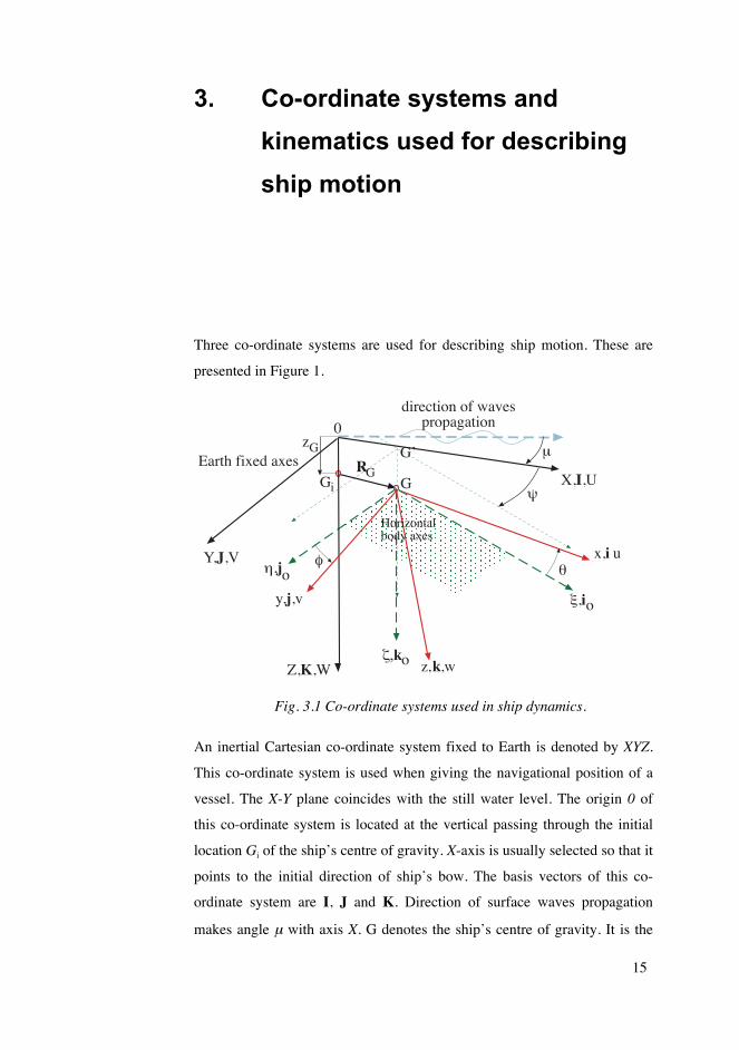
Three co-ordinate systems are used for describing ship motion. These are
presented in Figure 1.
Fig. 3.1 Co-ordinate systems used in ship dynamics.
An inertial Cartesian co-ordinate system fixed to Earth is denoted by XYZ.
This co-ordinate system is used when giving the navigational position of a
vessel. The X-Y plane coincides with the still water level. The origin 0 of
this co-ordinate system is located at the vertical passing through the initial
location Gi of the ship’s centre of gravity. X-axis is usually selected so that it
points to the initial direction of ship’s bow. The basis vectors of this co-
ordinate system are I, J and K. Direction of surface waves propagation
makes angle μ with axis X. G denotes the ship’s centre of gravity. It is the
Earth fixed axes G’
,j
k
,i
o
o
o
direction of wavespropagation
RG
zG
iG
x,i u
z,k,w
G X,I,U
Y,J,V
Z,K,W
0
Horizontalbody axes
y,j,v

16
origin of the moving Cartesian co-ordinate system xyz fixed with the ship
with the x-axis pointing towards the bow. This system is called the body-
fixed co-ordinate system. The basis vectors of this body-fixed co-ordinate
system are i, j and k. The so-called horizontal body axes co-ordinate system
(Hamamoto & Kim, 1993) denoted as ξηζ also moves also with the ship so
that the plane ξ−η is parallel to the still water plane X-Y. The axes X and ξ
make an angle ψ, which is the deviation from the initial course. The main
role of this auxiliary co-ordinate system is to enable a definition of the
angular orientation of the vessel. We also use this co-ordinate system to
define linear motion components. Namely, the motion along the ξ-axis is
called surge. The motion components along the η- and ζ-axes are called
sway and heave respectively.
When describing ship motion we are interested in its position in the inertial
co-ordinate system XYZ. The position of a rigid body is uniquely defined by
the position of a certain selected point (e.g. the origin) of the body and by
the angular orientation. Thus the position of a rigid body moving in three
dimensional space is uniquely defined by six quantities. These are called as
the generalized co-ordinates and denoted by X ={XG,YG,ZG,φ, θ,ψ}T.
It is convenient, as above, although not necessary, to select the body’s centre
of gravity as the origin. Thus the vector RG=XGI+YGJ+ZGK gives the
translational position of the body. The components (XG, YG and ZG) of this
vector are three of the generalized co-ordinates. The time differentiation of
the position vector yields the velocity of the origin of ship as
U =RG = XGI+YGJ+ ZGK = ui+ vj+wk . (3.1)
Here ˙ X G, ˙ Y G , ˙ Z G and u, v, w are the velocity components of the velocity U of
the ship’s centre of gravity with respect to the inertial system expressed in
the inertial and in the body-fixed system, respectively. In the marine field
the angular position of a vessel is given by the so-called modified Euler
angles (ψ, θ and φ in Fig. 3.1). The angular position means angular
orientation of the body with respect to the inertial co-ordinate system XYZ.

17
Euler angles are the remaining three generalized co-ordinates describing the
position of a rigid body. The angular position also rules the relation between
the velocity components of Equation 3.1 expressed in two different frames.
In order to obtain this relation, let us rotate the inertial co-ordinate system to
the orientation of the body-fixed system in the three subsequent stages as
shown in Fig. 3.2.
Fig. 3.2 Definition of the Euler angles as a sequence of three rotations.
Figures (a), (b) and (c) are represented so that the rotation axes z, y and x are
perpendicular to the plane of the paper.
We start with the co-ordinate system x3y3z3 having the origin in the body’s
centre of gravity and the angular orientation the same as that of the inertial
co-ordinate system XYZ. We rotate this system (see Fig. 3.2a) through the
angle ψ about the axis z3. As a result we get the co-ordinate system x2y2z2.
This angle is called the yaw.
The relation of the velocity components between these two co-ordinate
systems can be expressed as follows (Fossen, 1994; Clayton&Bishop, 1982;
Salonen, 1999).
(3.2)
The subsequent rotations (pitch and roll) about the y- and x-axis respectively
(see figures 3b and 3c) yield the transformations
u3v3w3
⎧
⎨⎪
⎩⎪
⎫
⎬⎪
⎭⎪=
cosψ − sinψ 0
sinψ cosψ 0
0 0 1
⎡
⎣
⎢⎢⎢
⎤
⎦
⎥⎥⎥
u2v2w2
⎧
⎨⎪
⎩⎪
⎫
⎬⎪
⎭⎪

18
(3.3)
Combining (3.2) and (3.3) and noting that the velocity components in the
x3y3z3 co-ordinate system are the same as those of the XYZ inertial system,
the one gets
XG
YG
ZG
⎧
⎨⎪⎪
⎩⎪⎪
⎫
⎬⎪⎪
⎭⎪⎪
=
cosψ cosθcosψ sinθ sinφ
−sinψ cosφ
cosψ sinθ cosφ
+sinψ sinφ
sinψ cosθsinψ sinθ sinφ
+cosψ cosφ
sinψ sinθ cosφ
−cosψ sinφ
−sinθ +cosθ sinφ cosθ cosφ
⎡
⎣
⎢⎢⎢⎢⎢⎢
⎤
⎦
⎥⎥⎥⎥⎥⎥
uvw
⎧
⎨⎪
⎩⎪
⎫
⎬⎪
⎭⎪
=T1 γ( )uvw
⎧
⎨⎪
⎩⎪
⎫
⎬⎪
⎭⎪.
(3.4)
with T1 being the transformation matrix from the body co-ordinate system to
the inertial co-ordinate system. Transformation matrix is dependent upon the
Euler angles (γ depicts the Euler angles).
Angular velocity ΩΩ of the ship in the body fixed co-ordinate system is
(3.5)
where p, q and r are the respective x-, y- and z-directional components of the
angular velocity. The dependence of the derivatives of the Euler angles and
angular velocity components of (3.5) is as follows (Fossen, 1994;
Clayton&Bishop, 1982)
u2v2w2
⎧
⎨⎪
⎩⎪
⎫
⎬⎪
⎭⎪=
cosθ 0 sinθ0 1 0
− sinθ 0 cosθ
⎡
⎣
⎢⎢⎢
⎤
⎦
⎥⎥⎥
u1v1w1
⎧
⎨⎪
⎩⎪
⎫
⎬⎪
⎭⎪
u1v1w1
⎧
⎨⎪
⎩⎪
⎫
⎬⎪
⎭⎪=
1 0 00 cosφ − sinφ0 sinφ cosφ
⎡
⎣
⎢⎢⎢
⎤
⎦
⎥⎥⎥
uvw
⎧⎨⎪
⎩⎪
⎫⎬⎪
⎭⎪
= pi + qj+ rk,

19
φ
θψ
⎧
⎨⎪
⎩⎪
⎫
⎬⎪
⎭⎪=
1 sinφ tanθ cosφ tanθ
0 cosφ −sinφ
0 sinφ / cosθ cosφ / cosθ
⎡
⎣
⎢⎢⎢
⎤
⎦
⎥⎥⎥
p
q
r
⎧
⎨⎪
⎩⎪
⎫
⎬⎪
⎭⎪=T2 (γ )
p
q
r
⎧
⎨⎪
⎩⎪
⎫
⎬⎪
⎭⎪
(3.6)
with T2 being the transformation matrix of the angular velocities in the
body-fixed co-ordinate system to the angular velocities expressed using the
Euler angles. This matrix is also dependent upon the Euler angles.
A shorter notation for a relation between the velocities expressed in two
frames can be used:
X =T1 γ( ) 03×3
03×3 T2 γ( )
⎡
⎣
⎢⎢
⎤
⎦
⎥⎥x
(3.7)
where vector
X =
Uγ
⎧⎨⎪
⎩⎪
⎫⎬⎪
⎭⎪= XG ,YG ,ZG ,φ,θ ,ψ{ }
T
(3.8)
comprises both the velocity components in the Earth-fixed co-ordinate
system and the time derivatives of the Euler angles. The matrices 03x3 are of
a size three times three and they comprise zeros. Vector
x = U
Ω
⎧⎨⎩
⎫⎬⎭= u,v,w, p,q,r{ }
T
(3.9)
comprises both the linear and the angular velocities in the moving body-
fixed co-ordinate system.

20
4. General form of equations of
motion
The general equations of motion of a rigid body can be described by two
vector equations.
4.1 Equations of translational motion
The translational motion describing the motion of ship origin G stems from
Newton's second law and is of the form
(4.1)
where F is the vector of the external forces, m is the mass of a rigid body
and U is the velocity of the centre of gravity of the body with respect to the
inertial co-ordinate system. It is not easy to express external forces acting on
a ship in the inertial XYZ co-ordinate system. It is easier and more logical to
have them expressed in the co-ordinate system moving with the ship, that is,
in the body-fixed system. Equation (4.1) expressed in the body-fixed co-
ordinate system xyz is (Salonen, 1999)
(4.2)
where δ/δt denotes the time derivative in the moving co-ordinate system. It
is feasible to separate the gravity mgK and other forces X,Y and Z from the
total force vector F. Thus
(4.3)
F =mdUd t,
F ==tmU( ) + mU,
F == Xi + Yj+ Zk + mgK.

21
Note that the reaction forces X,Y and Z are given in the body-fixed co-
ordinate system xyz. With a separation of external forces presented above
the vector equation (4.2) can be expressed in the component form as follows
(Clayton&Bishop, 1982)
(4.4)
It is interesting to note that the angular motion of a ship causes nonlinear
cross-coupling velocity terms to appear in the equations of a translational
motion.
Sometimes it is more convenient to have the origin of the body-fixed co-
ordinate system located somewhere else than at the centre of gravity. In ship
dynamics this point may be located for instance at the intersection of three
planes: the main frame, the centreplane and the waterplane. If we denote by
the position of the ship’s centre of gravity in the new
body fixed coordinate system, then the component equations of (4.2) appear
as (Triantafyllou& Hover, 2003):
m u+qw− rv+qzG − ryG + qyG + rzG( ) p− q2 + r2( ) xG⎡⎣
⎤⎦
= X −mgsinθ
m v+ ru − pw+ rxG − pzG + rzG + pzG( )q− r2 + p2( ) yG⎡⎣
⎤⎦
=Y +mgcosθ sinφ
m w+ pv−qu+ pyG −qxG + pxG +qyG( )r − p2 +q2( ) zG⎡⎣
⎤⎦
= Z +mgcosθ cosφ.
(4.4a)
Here, u, v and w are now the velocity components of the new origin.
4.2 Equations of angular motion
The angular motion is governed by the vector equation
(4.5)
m ˙ u ++ qw rv(( ) = X mgsin
m ˙ v + ru pw( ) = Y + mgcos sin
m ˙ w + pv qu( ) = Z + mgcos cos .
rG == xGi + yG j+ zGk
G =dhdt
=ht+ h

22
where G = Ki + Mj + Nk is the moment of external forces about the centre
of gravity and h is the angular momentum given in the form
h =
I ⋅ ΩΩ =Ix -Ixy -Ixz-Iyx Iy -Iyz-Izx -Izy Iz
⎡
⎣
⎢ ⎢ ⎢
⎤
⎦
⎥ ⎥ ⎥
p
q
r
⎧ ⎨ ⎪
⎩ ⎪
⎫ ⎬ ⎪
⎭ ⎪
(4.6)
Matrix
I comprises the elements of the mass moment of inertia of the body.
If we assume that the considered body consists of N masses mi, the
definitions of the elements of matrix
I are:
Diagonal terms Cross-inertia terms
(4.7)
Equation (4.5) in the component form is (Clayton&Bishop, 1982)
(4.8)
For the origin located off the ship’s centre of gravity but with axes of a new
co-ordinate system parallel to the original one, equations of the angular
motion get somewhat more complicated form (Fossen, 1994):
Ix == mi yi2 + zi
2( )i=1
N
Iy = mi xi2 + zi
2( )i=1
N
Iz = mi xi2 + yi
2( )i=1
N
Ixy == Iyx = mixi yii=1
N
Ixz = Izx = mixizii=1
N
Iyz = Izy = miyizii=1
N
.
Ix ˙ p −− Ixy ˙ q − Ixz ˙ r + Izr − Izx p − Izyq( )q − Iyq − Iyzr − Iyx p( )r = K
Iy ˙ q − Iyx ˙ p − Iyz ˙ r + Ix p − Ixyq − Ixzr( )r − Izr − Izx p − Izyq( ) p = M
Iz ˙ r − Izx ˙ p − Izy ˙ q + Iyq − Iyzr − Iyx p( ) p − Ix p − Ixyq − Ixzr( )q = N.

23
(4.9)
Moreover, the elements of the mass moment of inertia of the body used in
4.9 are changed according to Steiner’s rule as follows
Ix = Ix( )G+m yG
2 + zG2( )
Iy = Iy( )G+m xG
2 + zG2( )
Iz = Iz( )G+m xG
2 + yG2( )
Ixy = Ixy( )G+mxGyG
Iyz = Iyz( )G+myGzG
Izx = Izx( )G+mzGxG ,
(4.10)
with the moment of inertia terms on RHS being defined by Equation 4.7 in
the co-ordinate system having the origin in the Centre of Gravity G.
Equations (4.8) or (4.9) yield the angular motion of the body in terms of
angular velocity components p, q and r expressed in the moving co-ordinate
system xyz. These equations and expressions (4.4) are the final equations
governing total rigid body motion in six degrees of freedom. In order to
solve them we need to specify the external (fluid) forces X,Y,Z and moments
K,M,N acting on a body. Moreover we use equations (3.4) and (3.6) to
express body velocities in the inertial co-ordinate system. Numerical
integration of these equations yields the instantaneous position and
orientation of a ship in the inertial co-ordinate system XYZ.
The main problem of ship dynamics is not really in the equations of motion
as such. The main issue is to construct the appropriate mathematical models
describing the external (fluid) forces F and moments G caused by waves, by
Ix ˙ p Ixy ˙ q Ixz ˙ r + Izr Izx p Izyq( ))q Iyq Iyzr Iyx p( )r
+m yG ˙ w uq + vp( ) zG ˙ v wp + ur( )[ ] = K
Iy ˙ q Iyx ˙ p Iyz ˙ r + Ix p Ixyq Ixzr( )r Izr Izx p Izyq( ) p
+m zG ˙ u vr + wq( ) xG ˙ w uq + vp( )[ ] = M
Iz ˙ r Izx ˙ p Izy ˙ q + Iyq Iyzr Iyx p( ) p Ix p Ixyq Ixzr( )q
+m xG ˙ v wp + ur( ) yG ˙ u vr + wq( )[ ] = N .

24
the ship-to-water interaction or caused by other factors. Thus the problem is
in hydrodynamics.
25
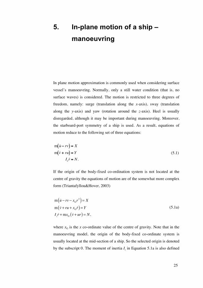
5. In-plane motion of a ship – manoeuvring
In plane motion approximation is commonly used when considering surface
vessel’s manoeuvring. Normally, only a still water condition (that is, no
surface waves) is considered. The motion is restricted to three degrees of
freedom, namely: surge (translation along the x-axis), sway (translation
along the y-axis) and yaw (rotation around the z-axis). Heel is usually
disregarded, although it may be important during manoeuvring. Moreover,
the starboard-port symmetry of a ship is used. As a result, equations of
motion reduce to the following set of three equations:
(5.1)
If the origin of the body-fixed co-ordination system is not located at the
centre of gravity the equations of motion are of the somewhat more complex
form (Triantafyllou&Hover, 2003)
m u − rv − xGr2( ) = X
m v + ru + xGr( ) = YIzr +mxG v + ur( ) = N ,
(5.1a)
where xG is the x co-ordinate value of the centre of gravity. Note that in the
manoeuvring model, the origin of the body-fixed co-ordinate system is
usually located at the mid-section of a ship. So the selected origin is denoted
by the subscript 0. The moment of inertia Iz in Equation 5.1a is also defined
m ˙ u rv( ) = X
m ˙ v + ru( ) = Y
Iz ˙ r = N .

26
in the same co-ordinate system. If the moment of inertia related to the
Centre-of-Gravity G is used, then the equations of motion are of the form
m u − rv − xGr2( ) = X
m v + ru + xGr( ) = YIz +mxG
2( )r +mxG v + ur( ) = N .
(5.1b)
5.1 Slow motion approximation for the hydrodynamic forces
The hydrodynamic forces X, Y and moment N consist mainly of the forces
acting on the hull and of the forces generated by the control surfaces
(rudders, propellers, etc.) of a vessel. In principle there are three basic
models used in describing hull forces. In the manoeuvring theory, it is
customary to use the so-called slow motion derivatives model for hull
forces. This approach does not attempt to model the physics of the
complicated flow over the manoeuvring hull. It is simply assumed that the
forces are dependent upon the motion variables (u, v and r), their time
derivatives, hull geometry and the rudder angle δ. The Taylor series
expansion of forces is used. In detail, the following expression, illustrated
with the aid of a two-variable function f=f(x,y), is used:
f (h,k) = f (0,0) + ∂f (0,0)∂x
h + ∂f (0,0)∂y
k
+ 12
∂ 2 f (0,0)∂x 2
h2 + 2∂2 f (0,0)∂x∂y
hk + ∂ 2 f (0,0)∂y 2
k 2⎛
⎝ ⎜
⎞
⎠ ⎟ +16.....( ) + R3
(5.5)
5.2 Linear model of a ship’s in-plane motion
The x-directional vessel velocity is decomposed into the initial constant U
and the perturbed part u as follows:
u := U + u, where |u|<<U. (5.6)
Moreover, sway velocity is assumed to be much smaller than the forward
ship speed that is v <<U. Thus in the following u means the deviation from

27
the initial velocity U. The linear model of ship manoeuvring is obtained by
dropping the nonlinear terms in the equations of motion (5.1a), as follows:
(5.7)
In general, the linear approximations of X, Y and N are:
Xlin = Xuu + Xuu + Xvv + Xvv + Xrr + Xrr + XδδYlin = Yuu +Yuu +Yvv +Yvv +Yrr +Yrr +YδδNlin = Nuu + Nuu + Nvv + Nvv + Nrr + Nrr + Nδδ .
(5.8)
In (5.8), the so-called hydrodynamic derivatives are used, as in the following
example
X ˙ u ≡∂X
∂˙ u ,Yu ≡
∂Y
∂u,Y ˙ u ≡
∂Y
∂˙ u ,etc
and δ is the rudder angle.
As a result the following set of three linear equations of motions is obtained:
X ˙ u - m( ) ˙ u + Xuu + X ˙ v ˙ v + Xvv + X ˙ r + Xrr + Xδδ = 0
Y ˙ u ˙ u + Yuu + Y ˙ v - m( ) ˙ v + Yvv + Y˙ r − mxG( ) ˙ r + Yr − mU( )r + Yδδ = 0
N ˙ u ˙ u + Nuu + N ˙ v − mxG( ) ˙ v + Nvv + N ˙ r − Iz( ) ˙ r + Nr − mxGU( )r + Nδδ = 0.
(5.9)
The terms
(5.10)
are known as added masses. The name stems from the fact that accelerating
the body entrained by the fluid requires a larger force than the
corresponding force needed to achieve the same acceleration in the vacuum
or in a gas. Thus the effect of the fluid entraining the accelerated body is the
same as that of the mass of a body. This means that in a sense the
surrounding fluid increases the mass of a body by an amount called added
m ˙ u == Xlin
m ˙ v + Ur + xG ˙ r ( ) = Ylin
Iz ˙ r + mxG ˙ v + Ur( ) = Nlin,
X ˙ u , Y˙ v and N ˙ r

28
mass. Added masses and moments of inertia of the typical ship shapes have
positive values of the same order of magnitude as the corresponding ship’s
quantities. More on this subject is dealt with in Section 6.3.
The terms
depict the influence of sway and yaw motion on the x-directional force
acting on a hull. This influence is usually disregarded. Also the effect of
rudder deflection on the ship resistance is in most cases not taken into
account, i.e. Xδ=0. The effect of surge motion on sway force Y and yaw
moment N are usually disregarded as well, that is:
Next, let us examine the nature of the remaining terms:
(5.11)
The first of these, Xu multiplied by the velocity change u, gives the change
in the force component X. Ship resistance, which is a negative force
component X, increases with ship speed. Thus Xu has to be negative. The
physical meanings of the other terms are explained with the aid of Figure
5.1.
Fig. 5.1 Forces acting on a ship in an oblique flow.
X ˙ v ,Xv ,X ˙ r and Xr
Y˙ u == Yu = N ˙ u = Nu = 0.
Xu,Yr ,Yv,Nv ,Nr,Y and N .

29
Apart from the bow-wards oriented velocity u, if a ship also has y-
directional velocity v, the inflow to the hull resembles the flow over a low
aspect ratio airfoil set at angle of attack β. Angle β is actually a drift angle
of the ship. As a result of an oblique flow, a negative side force Y develops.
This force acts normally at some point N located between the stem (extreme
bow) and mid-ship. Moving this force to the origin 0 results in a yawing
moment, N = Y xN. It is clear from Figure 5.1 that for the positive v-motion
of a ship, both the side force Y and the yaw moment N are negative. Thus
both terms Yv and Nv have to be negative, too. For a positive pure yaw
motion the opposing yaw moment also has to be negative. Thus the term Nr
has to be negative, too. It is not possible to give a general conclusion about
the sign of Yr in this situation.
5.3 Straight line stability
Next we consider a ship represented by a linear manoeuvring model (5.9)
and with the rudder fixed to the neutral positional; that is, the following
equations have to be considered
(5.12)
The surge equation was dropped because in the linear form it does not affect
other equations. As a result two linear homogeneous differential equations
(5.12) of the first order were obtained. These can be presented in matrix
form as follows:
(5.13)
or in a phase plane (v, r) as
(5.14)
where the aij coefficients are:
Y˙ v - m(( ) ˙ v + Yvv + Y˙ r mxG( ) ˙ r + Yr mU( )r = 0
N ˙ v mxG( ) ˙ v + Nvv + N ˙ r Iz( ) ˙ r + Nr mxGU( )r = 0.
Y˙ v - m Y˙ r mxG
N ˙ v mxG N ˙ r Iz
˙ v
˙ r
=
Yv mU Yr
Nv mxGU Nr
v
r
˙ v == a11v + a12r
˙ r = a21v + a22r,
30
(5.15)
Differentiating the first of the equations (5.14) yields:
v = a11v + a12r . (5.16)
Moreover, the first of the equations (5.14) can be written as
a12r = v−a11v . (5.14c)
Substituting into the equation (5.16) the second of the equations (5.14) and
equation (5.14c) as follows
v = a11v+a12r = a11v+a12 a21v+a221
a12v−a11v( )
⎡
⎣⎢
⎤
⎦⎥
= a11v+a12a21v+a22v−a22a11v
(5.17)
yields a homogeneous linear ordinary differential equation
v− a11 +a22( )v+ a11a22 −a12a21( )v = 0 (5.17a)
having solutions of the form eλt or teλt, where t is time and λ is a
characteristic value. As a result, the sway equation can be presented as the
characteristic equation
λ2 − a11 + a22( )λ + a11a22 − a12a21 = 0 (5.18)
a11 ==Iz N ˙ r ( )Yv + Y˙ r mxG( )Nv
m Y˙ v ( ) Iz N ˙ r ( ) mxG Y˙ r ( ) mxG N ˙ v ( )
a12 =Iz N ˙ r ( ) mU Yr( ) Y˙ r mxG( ) mxGU Nr( ))m Y˙ v ( ) Iz N ˙ r ( ) mxG Y˙ r ( ) mxG N ˙ v ( )
a21 =N ˙ v mxG( )Yv + m Y˙ v ( )Nv
m Y˙ v ( ) Iz N ˙ r ( ) mxG Y˙ r ( ) mxG N ˙ v ( )
a22 =N ˙ v mxG( ) mU Yr( ) m Y˙ v ( ) mxGU Nr( )m Y˙ v ( ) Iz N ˙ r ( ) mxG Y˙ r ( ) mxG N ˙ v ( )
.

31
The solution of the sway equation (5.17a) is stable if the real valued roots
λ1 and λ2 of the characteristic equation (5.18) are negative. If roots λ are
complex values then their real part has to be negative in order to insure the
straight line stability. This requires that the following holds (Kreyszig,
1993)
(5.19)
The first condition of the straight line stability is obtained using the first of
the conditions (5.19), the definitions (5.15) of the constants a11 and a22 and
assuming that the mass centre is close to the geometrical centre, i.e. xG≈0.
Moreover, the coupling terms
are small when compared to the other terms. As the terms ,
the common denominator of equations (5.15) is positive and thus can be
disregarded. The terms depicting drag (Yv and Nr) are both large negative
values. As a result the following terms:
(5.20)
and the first of the stability conditions (5.19) are fulfilled. The second of the
conditions (5.19) results in the following
a11 a22 > 0
a11a22 a12a21 > 0.
Y˙ r ,Yr ,N ˙ v and Nv
Y˙ v -m,N ˙ r -Iz
a11 ==Yv
m Y˙ v < 0
a22 =Nr
Iz N ˙ r < 0

32
Iz − Nr( )Yv + Yr −mxG( )Nv⎡⎣ ⎤⎦ − Nv −mxG( ) mU −Yr( )− m −Yv( ) mxGU − Nr( )⎡⎣ ⎤⎦+ Iz − Nr( ) mU −Yr( ) + Yr −mxG( ) mxGU − Nr( )⎡⎣ ⎤⎦ Nv −mxG( )Yv + m −Yv( )Nv⎡⎣ ⎤⎦= − Iz − Nr( )Yv Nv −mxG( ) mU −Yr( ) + Iz − Nr( ) mU −Yr( ) Nv −mxG( )Yv− Iz − Nr( )Yv m −Yv( ) mxGU − Nr( ) + Iz − Nr( ) mU −Yr( ) m −Yv( )Nv
− Yr −mxG( )Nv Nv −mxG( ) mU −Yr( ) + Yr −mxG( ) mxGU − Nr( ) Nv −mxG( )Yv− Yr −mxG( )Nv m −Yv( ) mxGU − Nr( ) + Yr −mxG( ) mxGU − Nr( ) m −Yv( )Nv
= Iz − Nr( ) m −Yv( ) Yv Nr −mxGU( ) + mU −Yr( )Nv⎡⎣ ⎤⎦− Yr −mxG( ) Nv −mxG( ) Yv Nr −mxGU( ) + mU −Yr( )Nv⎡⎣ ⎤⎦ > 0.
(5.21)
The first part of the expression (5.21) is obviously much bigger than the
second one because
As the term
is positive and large, the second condition of straight line stability can be
simplified by
(5.22)
The expression (5.22) is called the vessels stability criterion. If the ship’s
centre of gravity G is located very close to mid-ship then xG ≈ 0 and the
second stability condition simplifies further to
(5.23)
As already stated, Yv and Nr are both large negative values so their product is
positive. From (5.22) we can see that locating the centre of gravity bow-
wards of mid-ship (which means that xG > 0) increases directional stability.
The term Nv is usually negative. The surface area aft in a form of the keel or
projected hull area increases Nv, improving the directional stability.
Iz N ˙ r ( ) m Y˙ v ( ) >> Y˙ r mxG( ) N ˙ v mxG( )
Iz N ˙ r ( ) m Y˙ v ( )
Yv Nr mxGU( ) + mU Yr( )Nv > 0.
YvNr ++ mU Yr( )Nv > 0.

33
5.4 Non-linear model of ship maneuvering
When expressing the external forces dependent upon the motion variables,
the expansion factorials (1/2 and 1/6) of (5.5) are usually dropped. It is
assumed that the external hull forces are independent of the initial speed U.
Moreover, the symmetry properties are used. These for the X, that is for the
x-directional force component mean that it is (Triantafyllou et al, 2004):
a. a symmetric function of v when r=0 and δ =0, that is
X(u,v,r = 0, δ=0) = X(u,−v,r = 0, δ=0) and Xvvv=0.
b. a symmetric function of r when v=0 and δ =0,
c. a symmetric function of δ when v=0 and r=0.
Thus as a result this force can be expressed as follows:
(5.24)
In the case of the Y-force, hull symmetry implies that it has to be anti-
symmetric in respect to v when r=δ=0; and likewise for r and δ, i.e.
(Triantafyllou et al, 2004) and thus for instance
Y(u,v,r = 0, δ=0) = -Y(u,-v,r = 0, δ =0). The even derivatives of Y in respect
to v, r and δ must be zero, that is:
(5.25)
As a result the following expression for the Y-force is obtained:
(5.26)
X = X ˙ u ˙ u + Xuu + Xuuu2+ Xuuuu
3+ Xvvv
2+ Xrrr
2+ X 2
+Xvrvr + Xv v + Xr r + Xvvuv2u + Xrrur
2u + X u2u
+Xr ur u+ Xrvurvu + Xv uv u + Xr vr v.
Yvv = 0, Yvvu = 0, Yrr = 0, Yrru = 0, Yrru = 0, Y = 0,Y u = 0.
Y = Yuuu2
+ Y ˙ v ˙ v + Y˙ r ˙ r + Yvv + Yrr + Y + Y u u + Yvuvu + Yruru + Yvuuvu2
+Yruuru2+ Y uu u2
+ Yvvvv3
+ Yrrrr3
+ Y 3+ Yrr r2
+ Yvrrvr2
+Yrvvrv 2+ Y vv v 2
+ Yv r vr + Y r2r + Y v
2v.
34
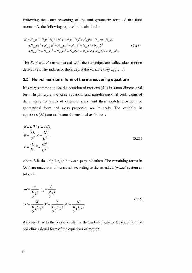
Following the same reasoning of the anti-symmetric form of the fluid
moment N, the following expression is obtained:
N = Nuuu2 + Nvv+ Nrr + Nvv+ Nrr + Nδδ + Nδuδu+ Nvuvu+ Nruru
+Nvuuvu2 + Nruuru
2 + Nδuuδu2 + Nvvvv
3 + Nrrrr3 + Nδδδδ
3
+Nrrδr2δ + Nvrrvr
2 + Nrvvrv2 + Nδvvδv
2 + Nvrδvrδ + Nδδrδ2r + Nδδvδ
2v.
(5.27)
The X, Y and N terms marked with the subscripts are called slow motion
derivatives. The indices of them depict the variable they apply to.
5.5 Non-dimensional form of the maneuvering equations
It is very common to use the equation of motions (5.1) in a non-dimensional
form. In principle, the same equations and non-dimensional coefficients of
them apply for ships of different sizes, and their models provided the
geometrical form and mass properties are in scale. The variables in
equations (5.1) are made non-dimensional as follows:
(5.28)
where L is the ship length between perpendiculars. The remaining terms in
(5.1) are made non-dimensional according to the so-called ‘prime’ system as
follows:
(5.29)
As a result, with the origin located in the centre of gravity G, we obtain the
non-dimensional form of the equations of motion:
u'== u /U,v'= v /U,
˙ u '=˙ u L
U 2 , ˙ v '=˙ v L
U 2 ,
r'=rL
U, ˙ r '=
˙ r L2
U 2 ,
m'==m
2L3,I'z =
Iz
2L5
X '=X
2L2U2
,Y '=Y
2L2U2
,N '=N
2L3U2
.

35
(5.30)
The same equations are obtained using instead of L2 a product of ship length
and draft T that is LT. In the so-called ‘bis’ system mass properties and
forces are made non-dimensional using the actual ship mass ρ∇, with
ρ being water density and ∇ being volumetric displacement.
5.6 Determination of the slow motion hydrodynamic derivatives
The knowledge of the hydrodynamic derivatives is crucial for a successful
prediction of ship’s manoeuvring. A normal approach in evaluating them
relies on dedicated captive model tests. These are:
Straight-line test with a model set at a certain drift.
The so-called rotating arm test.
Planar motion mechanism tests (PMM).
In these tests, the model is set at a certain steady position or forced to
conduct a prescribed regular (sinusoidal) motion. Propeller loading and
rudder angle may belong to the varied parameters as well. Knowing these
and measuring the forces acting on the model hull makes it possible to
evaluate a set of hydrodynamic derivatives. The tests are tedious and require
many test runs.
Last years’ rapid development of Computational Fluid Dynamics (CFD) in
evaluating the flows over the ships’ hulls also makes possible (in principle)
a numerical evaluation of the forces acting on the hull in a slow three-
dimensional motion. However, for the time being, this approach is very
limited and it is not used on a routine basis.
Tests with free-running radio-controlled models and sea-trial full-scale tests
are sometimes used to evaluate some of the hydrodynamic derivatives with
the aid of system identification techniques.
m' ˙ u ' r'v '( ) = X '
m' ˙ v '+ r'u'( ) = Y '
I'z ˙ r '= N ' .

36
Regression analysis conducted using the experimentally (model tests)
obtained data gives a first approximation of the linear hydrodynamic
derivatives as a function of principal dimensions (Brix, 1993):
Y 'v ' = −π T / L( )2 1+0.16CBB /T −5.1 B / L( )2⎡⎣
⎤⎦
Y 'r ' = −π T / L( )2 0.67B / L −0.0033 B /T( )2⎡⎣
⎤⎦
N 'v ' = −π T / L( )2 1.1B / L −0.041B /T[ ]
N 'r ' = −π T / L( )2 1 /12+0.017CBB /T −0.33B / L[ ]
Y 'v ' = −π T / L( )2 1+0.4CBB /T( )Y 'r ' = −π T / L( )2 −1/ 2+2.2B / L −0.08B /T( )N 'v ' = −π T / L( )2 1 / 2+2.4T / L( )N 'r ' = −π T / L( )2 1 / 4+0.039B /T −0.56B / L( ),
(5.31)
where CB is the volumetric block coefficient. The expressions (5.31)
represent the linear approximation to the hull derivatives in the body-fixed
co-ordinate system with the origin located at the mid-section. Formulas
(5.31) are not very accurate ones. They can be used as such when evaluating
stability derivatives for a new-building and can be applied when evaluating
the effect of ship’s main dimensions on the hydrodynamic derivatives. In
other words, if we have the derivatives for a certain ship and want to use this
knowledge for a similar ship, with a slightly changed main dimensions, we
can use the above given expressions. Expressions 5.31 are derived for a ship
with an even keel. For ships with trim t (positive bow up), correction factors
to be applied to the linear even-keel velocity coefficients are (Brix, 1993):
Y 'v ' (t) = Y 'v ' 1+ 0.67t /T( )Y 'r ' (t) = Y 'r ' 1+ 0.80t /T( )N 'v ' (t) = N 'v ' 1− 0.27 t /T( )Y 'v ' / N 'v '⎡⎣ ⎤⎦N 'r ' (t) = N 'r ' 1+ 0.30t /T( ).
(5.32)
Another model of hull forces, which is particularly suitable for a drifting
vessel, is based on the so-called cross-flow resistance concept (Bertram,
2000). In this model the resistance per unit ship length is evaluated by

37
0.5ρTxvx2CD , where subscript x depicts the longitudinal position of a ship
section, and Tx and vx are the draft and transverse velocity at this section
respectively. The latter is given by vx = v+ xr . The forces and moments
exerted on the hull due to the cross-flow resistance can be obtained by the
integration of the sectional contributors as follows (Bertram, 2000)
XYKN
⎧
⎨⎪⎪
⎩⎪⎪
⎫
⎬⎪⎪
⎭⎪⎪
=1
2ρ
0−1zD−x
⎧
⎨⎪⎪
⎩⎪⎪
⎫
⎬⎪⎪
⎭⎪⎪
L
∫ v+ xr( ) v+ xr TxCDdx,
(5.33)
where zD is the z coordinate (measured downward from the centre of gravity
G of ship’s mass m) of the action line of the cross-flow resistance. For
typical cargo ship hull forms, this force acts about 65% of the draft above
the keel line (Bertram, 2000). Thus a constant (mean) value over ship length
of:
zD = zG − 0.65T. (5.34)
Note that the above model makes allowance for roll as a degree of freedom
in the manoeuvring simulation.
5.7 Ship resistance and propeller thrust
There are two ways to model ship resistance and propulsor action. The
simplest way is to assume that resistance and thrust are of the same
magnitude and do not change. If there is a change in a ship’s speed during
the manoeuvres, it is caused by the cross-coupling term r’v’ of Equation
5.30 and by Equation 5.24. Another model, the modular model, takes into
account the resistance with an operating propeller using the following
formula
X resistance = −RT / 1− t( ) = −0.5ρu2SCT / 1− t( ) (5.33)
where RT is total resistance and CT its coefficient, ρ water density, S wetted
surface of ship hull, t thrust deduction factor, and u depicts the ship’s

38
velocity in x-direction. The total resistance coefficient CT can be given in
tabular form as a function of a Froude number.
5.7.1 Hull resistance
If there is no information on the resistance coefficient available but
propulsion power PD at a certain speed is known, the following way of
evaluating the resistance can be used. The relation between the propulsion
power and the resistance
PD = PE /ηD = RTV /ηD (5.36)
is used, yielding
RT = PDηD /V (5.37)
where the propulsive efficiency (Matusiak, 1993) is given by a product of
open water, rotational and hull efficiencies i.e.
ηD = η0ηRηH = η0ηR
1− t1− w
.
(5.38)
If there is no better data available, the following can be assumed. The open
water and the rotational efficiencies of the propeller are assumed to be
η0=0.65 and ηR=1 respectively. The wake coefficient w and thrust deduction
factor t can be assumed to be as presented in Table 5.1 below
Table 5.1 Approximate values of the propulsion coefficients.
Single screw vessel Multi-screw vessel
Wake fraction w 0.25 0.05
Thrust deduction factor t 0.25 0.15
For small variations of forward speed u, ship’s resistance can be evaluated
using the expression 5.35 with the assumption of constant resistance

39
coefficient CT. If large ship speed variations are investigated than the
resistance coefficient as a function of speed or Froude number should be
used instead.
5.7.2 Propeller thrust
There are two simple models representing the thrust developed by a
propeller. The first one is appropriate for a fixed pitch propeller. Total thrust
is evaluated from a known open water characteristic of the propeller (KT-J
curve) as follows
Xprop = Zρn2D4KT (5.39)
where Z is the number of propellers, n is the propeller revolutions per
second, and D is the propeller's diameter. The initial value of propeller
revolutions should be adjusted so that a desired ship velocity is obtained for
the condition of still water and constant forward speed with no drift angle.
In other words the propeller revolutions should be derived from the
condition Xprop = −Xresistance. Depending on the type of propulsion machinery,
the revolutions are kept constant or adjusted to keep the advance coefficient
J=V(1-w)/(nD) constant.
For the controllable pitch propellers (“CPP”), the following simplifying
procedure can be used. The assumption of constant delivered power and
constant propulsive efficiency is made. The latter implies good control of
propeller pitch and disregards the efficiency losses for the off-design
operational conditions (approx. 10%). The above assumptions and Equation
(5.37) result in the following relation of thrust Xprop and ship’s speed
Xprop = PDη0ηR
V (1− w).
(5.40)
The relation 5.40 may lead to unrealistically high thrust values at low
speeds. The limiting value is known as the bollard pull.

40
5.7.3 Bollard pull estimate
The bollard pull of the propeller can be derived from the theory of ideal
propulsor (Matusiak, 1993). In this theory, the thrust developed by a
stationary propeller is given by
T = 12ρA0UA 0
2 = 12ρ πD
2
4UA 02 ,
(5.41)
where UA0 is the flow velocity induced by the propeller far downstream. The
propulsion power is related to UA 02 by the following formula
PD = 14ρA0UA 0
3 = 1
16ρπD2UA 0
3 .
(5.42)
Solving the induced velocity UA0 from formula 5.42 yields
UA0 =16PDρπD2
⎛
⎝⎜
⎞
⎠⎟
1/3
,
(5.43)
which substituted into the thrust expression 5.41 yields the bollard pull that
is the maximum attainable thrust
T =1
2ρπD2
4
16PDρπD2
⎛
⎝⎜
⎞
⎠⎟
2/3
= πρ / 23 PDD( )2/3 . (5.44)
Alternatively for an open propeller (no duct), the semi-empirical expression
T = 7.8 PDD( )2 / 3 (5.45)
can be used when evaluating the maximum thrust delivered by the propeller.
5.8 Rudder action
The effect of a rudder on the forces acting on a ship is shown in Fig. 5.2. A
rudder set at angle δ develops a positive y-directional force, which when
approximated by a linear model is
41
YR = Yδδ. (5.46)
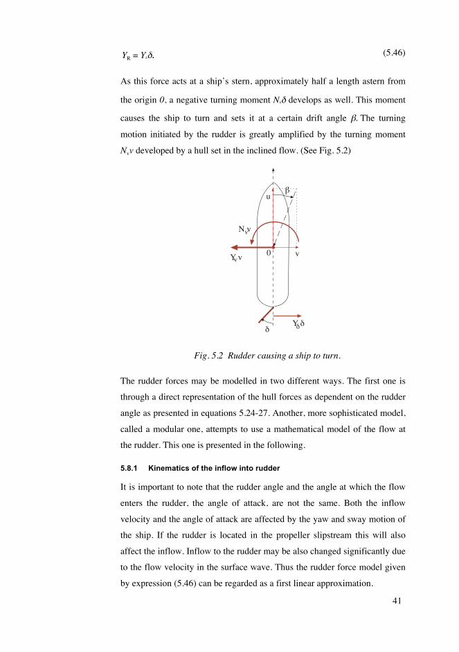
As this force acts at a ship’s stern, approximately half a length astern from
the origin 0, a negative turning moment Nδδ develops as well. This moment
causes the ship to turn and sets it at a certain drift angle β. The turning
motion initiated by the rudder is greatly amplified by the turning moment
Nvv developed by a hull set in the inclined flow. (See Fig. 5.2)
Fig. 5.2 Rudder causing a ship to turn.
The rudder forces may be modelled in two different ways. The first one is
through a direct representation of the hull forces as dependent on the rudder
angle as presented in equations 5.24-27. Another, more sophisticated model,
called a modular one, attempts to use a mathematical model of the flow at
the rudder. This one is presented in the following.
5.8.1 Kinematics of the inflow into rudder
It is important to note that the rudder angle and the angle at which the flow
enters the rudder, the angle of attack, are not the same. Both the inflow
velocity and the angle of attack are affected by the yaw and sway motion of
the ship. If the rudder is located in the propeller slipstream this will also
affect the inflow. Inflow to the rudder may be also changed significantly due
to the flow velocity in the surface wave. Thus the rudder force model given
by expression (5.46) can be regarded as a first linear approximation.
Y v 0
u
v
Y
v
N vv

42
In order to evaluate rudder forces the flow velocities at the rudder location
have to be evaluated first. A definition of the positive rudder angle is
presented in Fig. 5.2 along with the definition of rudder forces.
Fig. 5.3 Flow velocities at rudder.
Flow velocities at the rudder can be expressed as follows
, (5.47)
or explicitly as
Vx,R =Vx −Vx,wave + qzR − ryRVy,R = −v +Vy,wave − rxR + pzRVz,R = −w +Vz,wave − pyR + qxR ,
(5.48)
where Vx is the x-component of flow velocity in the slipstream of propeller.
This velocity can be evaluated as Vx= u*(1-w) knowing ship instantaneous
speed u and wake fraction w. Terms with subscript wave depict flow
velocities due to the wave action (Eq. 5.48). (xRyRzR) depicts the rudder
position in the body-fixed co-ordinate system. Note that the wave action is
seldom included in the manoeuvring modelling. It is included here for the
sake of completeness of the problem.
It is seen from Figure 5.3 that the effect of ship motion and the wave motion
is to change the angle of attack of the rudder by the amount
Vx,RVy,RVz, R
=
Vx Vx ,wavev + Vy ,wavew + Vz,wave
i j k
p q r
xR yR zR
43
(5.49)
so that the total angle of attack is α=δ+γ.
Rudder forces are evaluated according to Söding (1982) and Brix (1993).
Lift L and drag D forces are given by
(5.50)
where lift coefficient is given by
(5.51)
Here, Λ =b2/AR is the aspect ratio, where b denotes the rudder length. Note
that the rudder area is not a wetted area. It is defined as a projected area of
the side view of the rudder. The drag coefficient of the rudder is given by
(5.52)
where CD0 is the viscous drag coefficient. It can evaluated according to
ITTC-57 frictional resistance coefficient as follows
(5.53)
where Reynold's number is defined as
(5.54)
with c being the mean value of the rudder chord and ν being the kinematic
viscosity coefficient.
= arctan Vy,R /Vx,R( )
L =1
2CL ARVR
2, D =1
2CDARVR
2 ,
CL =2 +1( )
+ 2( )2 sin +( ),
CD =1.1CL2
+ CD0,
CD0 = 2.5CF = 2.50.075
log Rn 2( )2 ,
Rn =Vrudderc ,
44
5.8.2 The effect of propeller action on the rudder flow
A rudder operates usually in the propeller slipstream. As a result, the forces
developed by a rudder are substantially higher than the ones generated by a
rudder placed outside the slipstream. The flow velocity in the propeller
slipstream can be evaluated as follows.
According to the potential flow theory and considering the momentum
conservation (ideal propulsor model), the mean axial flow velocity far
downstream of the propeller is (Matusiak, 2005)
(5.55)
where VA is the advance velocity in the propeller plane, and the thrust
loading coefficient is given by
. (5.56)
Propeller diameter is denoted by D. According to this simple ideal propulsor
model, the radius of the slipstream far behind the propeller is given by
(5.57)
where r0 is the propeller radius. The limited distance x of the propeller and
rudder results in a smaller contraction of the slipstream radius r and a
smaller value of the axial velocity Vx in the slipstream at the position of the
rudder. These can be approximated by the following expressions
(5.58)
V = VA +UA0 = VA 1 + CT ,
CT =Thrust
0.5 VA2 D2 / 4
=8 KTJ2
r = r01
21+
VAV
,
r
r0=0.14 r /r0( )
3+ r /r0( ) x /r0( )
1.5
0.14 r /r0( )3
+ x /r0( )1.5
VxV
=r
r
2
.

45
Equations (5.57) are approximations based on potential flow theory.
Turbulent mixing of the water jet and surrounding flow increases the radius
of the slipstream by Δr. This effect is taken into account by the formula
(5.59)
and the corresponding, corrected axial velocity of flow in the slipstream is
(5.60)
The limited radius of the slipstream has a diminishing effect on the rudder
lift. This can be taken into account by multiplying the lift by the factor
(5.61)
where
(5.62)
5.9 Azimuth thruster as the main propulsor
Azimuth thruster units used as the main propulsion means have become very
popular in a variety of ship types within the last two decades. Very often
they are called podded propellers. There are several benefits in using them.
Apart from good manoeuvring qualities, ships equipped with this kind of
propulsor are claimed to be free of vibration and noise problems. The the
overall propulsion characteristics are also good, thanks to the absence of
propeller shafts and supporting brackets.
Perhaps the biggest difference in the action of podded propellers when
compared with traditional propellers is that they operate frequently in
oblique inflow. The knowledge of the forces developed by a propeller in an
oblique inflow is very important in order to evaluate ship’s manoeuvring. In
particular, stopping a vessel may be conducted quite differently and faster
than in the case of the traditional propulsion arrangement.
r = 0.15xVx VAVx +VA
Vcorr = (Vx VA )r
r + r
2
+VA .
= VA /Vcorr( )f with f = 2
2
2 + d /c
8
,
d = /4 r + r( ).

46
The model of the forces acting on the azimuth type thruster in the oblique
flow as outlined below is relatively simple. It addresses the problem of the
forces acting on a propeller only. It does not attempt to deal with the
hydrodynamic forces acting on the pod, strut and fins. A more elaborate
model, which includes all the elements of the podded propulsor, is presented
in Ruponen (2003) and Ruponen & Matusiak (2004). Oblique inflow to the
propeller disk involves a radical change in the forces acting on a propulsor.
Steady force components change. In particular, a significant in-plane
component Fpy of the total force develops (Matusiak, 2003b)
(5.63)
where Ap is the propeller disk area,
VA = Vx,R cosδ −Vy,R sinδ (5.64)
is propeller advance velocity,
Vpy = Vx,R sinδ +Vy,R cosδ (5.65)
is flow velocity in-plane of the propeller plane, and UA is the propeller-
induced velocity in this plane. Refer to the Figure 5.4 for definitions of flow
kinematics and the definition of the forces.
Fpy = Ap VA +UA( )Vpy,

47
Fig. 5.4 Flow kinematics and forces acting on the propeller in an oblique flow.
The propeller-induced velocity UA can be evaluated from the actuator disk
approximation of the propeller as follows
(5.66)
where the thrust loading coefficient CT is given by Formula (5.56).
The thrust of the propeller is evaluated from the known thrust coefficient KT
as a function of the advance ratio J=VA/(nD), where n and D are propeller
revolutions and diameter, respectively. Having both the thrust T and the in-
plane component Fpy of the total force evaluated, the force propelling the
ship Fx and rudder-like force Fy can be evaluated as follows:
(5.67)
A more profound discussion of rudder forces and propeller-rudder
interaction can be found in Molland&Turnock (2007). Luukkainen (2011)
has developed a model particularly suitable to simulate the manoeuvring of
cruise and RoPax vessels.
UA =VA 1+ 1+ CT( ) /2,
Fx = T cos Fpy sin
Fy = T sin + Fpy cos .
48
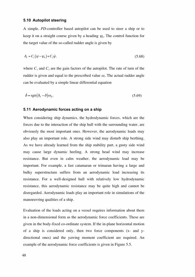
5.10 Autopilot steering
A simple, PD-controller based autopilot can be used to steer a ship or to
keep it on a straight course given by a heading ψ0. The control function for
the target value of the so-called rudder angle is given by
δT =C1 ψ −ψ0( )+C2ψ, (5.68)
where C1 and C2 are the gain factors of the autopilot. The rate of turn of the
rudder is given and equal to the prescribed value ωδ. The actual rudder angle
can be evaluated by a simple linear differential equation
δ = sgn δT −δ( )ωδ . (5.69)
5.11 Aerodynamic forces acting on a ship
When considering ship dynamics, the hydrodynamic forces, which are the
forces due to the interaction of the ship hull with the surrounding water, are
obviously the most important ones. However, the aerodynamic loads may
also play an important role. A strong side wind may disturb ship berthing.
As we have already learned from the ship stability part, a gusty side wind
may cause large dynamic heeling. A strong head wind may increase
resistance. But even in calm weather, the aerodynamic load may be
important. For example, a fast catamaran or trimaran having a large and
bulky superstructure suffers from an aerodynamic load increasing its
resistance. For a well-designed hull with relatively low hydrodynamic
resistance, this aerodynamic resistance may be quite high and cannot be
disregarded. Aerodynamic loads play an important role in simulations of the
manoeuvring qualities of a ship.
Evaluation of the loads acting on a vessel requires information about them
in a non-dimensional form as the aerodynamic force coefficients. These are
given in the body-fixed co-ordinate system. If the in-plane horizontal motion
of a ship is considered only, then two force components (x- and y-
directional ones) and the yawing moment coefficient are required. An
example of the aerodynamic force coefficients is given in Figure 5.5.

49
Fig. 5.5 Aerodynamic force coefficients and their dependence upon the angle
of the apparent wind.
When evaluating aerodynamic loads acting on a moving vessel one has to
take into account the varying orientation and velocity of the resulting
airflow. Figure 5.6 presents the components of the airflow components
making up the resulting wind vector Vwres.
Fig. 5.6 Air velocity components and aerodynamic force vectors acting on a
ship.
The wind blows with a velocity Vw from the direction making the angle α
with the X- axis of the inertial co-ordinate system. The projections of this
velocity vector on the body-fixed co-ordinate system x-y are
wind force coefficients
-1.2
-1
-0.8
-0.6
-0.4
-0.2
0
0.2
0.4
0.6
0.8
0 30 60 90 120 150 180
[deg]
C
Cx Cy 10*Cn

50
Vwx =Vw cos α +ψ( )Vwy =Vw sin α +ψ( ).
(5.70)
The resultant airflow velocity felt by a moving ship is given by the speed
Vwres = Vwx + u( )2 + Vwy − v( )2 (5.71)
and the angle ε made with the symmetry plane of a ship
ε = tan−1Vwy − vVwx + u .
(5.72)
The aerodynamic forces and moment are finally given by
Xwind = 0.5ρairATCXVwres2
Ywind = 0.5ρairALCYVwres2
Nwind = 0.5ρairALLCNVwres2 .
(5.73)
5.12 Numerical implementation of the maneuvering simulation
A modular simulation model using the linear hydrodynamic derivatives
5.31, ship resistance, propeller thrust and rudder models, as given in sections
5.6 and 5.7, is implemented in the form of the computer program ohjailu.f.
An allowance is made for autopilot steering and modelling the wind loads.
The origin is located in the mid-ship and the mass moment of inertia is
related to the Centre-Of-Gravity. The following equations of ship in-plane
motion are used
51
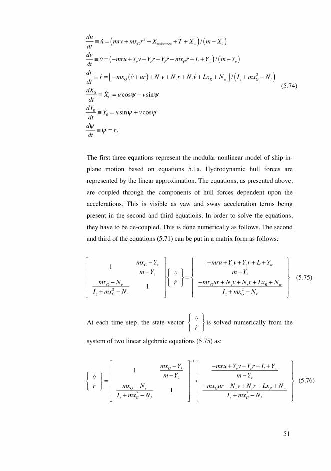
du
dt≡ u = mrv +mxGr
2 + Xresistance +T + Xw( ) / m − Xu( )dv
dt≡ v = −mru +Yvv +Yrr +Yrr −mxGr + L +Yw( ) / m −Yv( )
dr
dt≡ r = −mxG v + ur( ) + Nvv + Nrr + Nvv + LxR + Nw⎡⎣ ⎤⎦ / Iz +mxG
2 − Nr( )dX0dt
≡ X0 = u cosψ − vsinψ
dY0dt
≡ Y0 = u sinψ + vcosψ
dψdt
≡ψ = r.
(5.74)
The first three equations represent the modular nonlinear model of ship in-
plane motion based on equations 5.1a. Hydrodynamic hull forces are
represented by the linear approximation. The equations, as presented above,
are coupled through the components of hull forces dependent upon the
accelerations. This is visible as yaw and sway acceleration terms being
present in the second and third equations. In order to solve the equations,
they have to be de-coupled. This is done numerically as follows. The second
and third of the equations (5.71) can be put in a matrix form as follows:
1mxG −Yrm −Yv
mxG − Nv
Iz +mxG2 − Nr
1
⎡
⎣
⎢⎢⎢⎢⎢
⎤
⎦
⎥⎥⎥⎥⎥
vr
⎧⎨⎩
⎫⎬⎭=
−mru +Yvv +Yrr + L +Ywm −Yv
−mxGur + Nvv + Nrr + LxR + Nw
Iz +mxG2 − Nr
⎧
⎨⎪⎪
⎩⎪⎪
⎫
⎬⎪⎪
⎭⎪⎪
(5.75)
At each time step, the state vector vr
⎧⎨⎩
⎫⎬⎭
is solved numerically from the
system of two linear algebraic equations (5.75) as:
vr
⎧⎨⎩
⎫⎬⎭=
1mxG −Yrm −Yv
mxG − Nv
Iz +mxG2 − Nr
1
⎡
⎣
⎢⎢⎢⎢⎢
⎤
⎦
⎥⎥⎥⎥⎥
−1−mru +Yvv +Yrr + L +Yw
m −Yv−mxGur + Nvv + Nrr + LxR + Nw
Iz +mxG2 − Nr
⎧
⎨⎪⎪
⎩⎪⎪
⎫
⎬⎪⎪
⎭⎪⎪
(5.76)

52
Numerical integration is performed by the Runge-Kutta integration method
of fourth order. The solution of the first equation in 5.74 and the result of
integrating equations 5.76 is the velocity vector U=ui+vj of the ship’s origin
0 and yaw velocity r.
Integration of the three last equations of the set 5.74 yields ship’s position
X0(t),Y0(t),Ψ(t) in the inertial co-ordinate system X-Y. An example of the
simulated zigzag manoeuvre of Mariner ship is presented in Figure 5.7.
Fig. 5.7 Zigzag test of Mariner simulated with the program ohjailu.f. Initial
speed is 15 knots.
The result of the simulated turning circle manoeuvre is shown in Figure 5.8
below.
MARINER zig-zag tests 20/20
-30
-20
-10
0
10
20
30
0 60 120 180 240 300 360 420
Time [s]
YAW [deg] Rudder angle [deg]

53
Fig.5.8 Turning circle test of Mariner simulated with the program ohjailu.f.
Initial speed is 15 knots.
Speed drop during a turning circle manoeuvre is presented in Figure 5.9.
Fig. 5.9 Speed drop during a turning circle test of Mariner simulated with the
program ohjailu.f. Initial speed is 15 knots. Propeller revolutions are kept
constant.
Turning circle; rudder 20 deg
-100
0
100
200
300
400
500
600
700
800
900
-200 0 200 400 600 800 1000 1200 1400
X [m]
Y [
m]
Speed in turn
0
1
2
3
4
5
6
7
8
9
0 60 120 180 240 300 360 420 480 540 600
Time [s]
Spe
ed [
m/s
]

54
6. Sea surface waves
The water sea surface is seldom (if ever) completely still and flat. It is
mainly the interaction of wind and water that causes the free surface to
deform. As a result, surface waves form. We shall not deal with the
mechanism of generation of surface waves that is, we shall not treat the
physical mechanism of wave evolution. This can be found for instance in
Young (1999). Instead we shall present the classical, but still very much
applicable, small amplitude that is the linear theory of surface waves as first
presented by Airy.
Surface waves starting from the length of a few metres up to approximately
the length of 1 km are of interest in ship and offshore structural dynamics.
Apart these surface waves, there are much slower internal waves caused by
density stratification. Tides, caused by a change of the position of heavenly
bodies with respect to the Earth, are usually not important when considering
periodic loads and motions acting on ships. Capillary waves and ripples are
high frequency phenomena, which can be disregarded when dealing with
ship dynamics problems.
6.1 Plane progressive linear regular waves
The pattern of waves observed from a travelling ship is very complex. Apart
from the waves generated by the vessel itself, a large number of waves of
different length and height can be observed, each progressing in a different
direction. When we travel by air over the ocean and especially in the vicinity
of the coastal line, we observe that the wave pattern exhibits certain
regularities. The prevailing direction of wave progression is noticed, and the
length of the waves does not vary so much anymore. This observation
justifies modelling the sea surface waves as plane progressive ones. This is

55
done quite often in the model tests (see Fig. 6.1) and also in computational
methods.
Fig. 6.1 Model of a pilot boat in the steep regular unidirectional waves
generated in the multifunctional model basin of the Aalto University.
6.1.1 Assumptions and boundary conditions
The most common assumptions made when dealing with surface waves is
that the associated flow is ideal. This means that the flow is assumed to be
inviscid and irrotational. Thus the flow may be fully described by the
velocity potential φ = φ(X0,Y0,Z0) . Evaluation of this velocity potential rests
on fulfilment of the mass continuity equation, which is of the form of
Laplace equation
(6.1)
and on satisfying the boundary conditions of the flow in question. The most
important boundary conditions are these set by a free deforming surface.
When describing progressive waves we use a Cartesian co-ordinate system
with the origin 0 fixed in space and located on the undisturbed water
surface. The X0-axis points in the direction of waves propagation, while the
Z0-axis points vertically upwards. The vertical elevation of the free surface
is defined by
2
X02
+2
Y02 +
2
Z02 = 0

56
(6.2)
Kinematic boundary condition at the free surface
The so-called kinematic boundary condition can be obtained by requiring
that the substantial derivative of the quantity
F(X0,Y0,Z0,t)≡ Z0 −ζ (X0,Y0,t) is zero:
DF
Dt= ∂F∂t
+ v ⋅ ∇F = ∂∂t
Z0 −ζ (X0,Y0,t)[ ] + v ⋅ ∇ Z0 −ζ (X0,Y0,t)[ ]
= −∂ζ∂t
− u0∂ζ∂X0
− v0∂ζ∂Y0
+ w0
(6.3)
Here u0, v0 and w0 are X0-, Y0- and Z0- directional flow components
respectively. For the waves progressing in the X0-direction we can write
(6.3) as follows
w0 = ∂ζ∂t
+ u0∂ζ∂X0 .
(6.4)
The meaning of expression 6.4 is illustrated in Figure 6.2.
Fig. 6.2 Flow tangency condition at the free surface.
Z0 = (X0,Y0,t).

57
It is clearly seen that with the free surface being frozen, ( ) (6.4)
means the tangency condition of the flow at the free surface. For the
unsteady free surface motion the vertical flow velocity also takes into
account the vertical velocity component of the free surface deformation. In
both cases the kinematic boundary condition implies the tangency of the
flow velocity at the free surface. It is worth noting that the equation of the
kinematic condition derived above also applies to the viscous and rotational
flows as well.
Making use of the fact that the slopes of the surface water waves are small,
the linearized kinematic boundary condition can be obtained by dropping
the terms involving spatial derivatives of wave elevation and evaluating it
approximately at Z0=0. Using the velocity potential the linearized
kinematical boundary condition is
∂ζ∂t
= ∂φ∂Z0
at Z0 = 0.
(6.5)
Dynamic boundary condition at the free surface
Neglecting surface tension, the dynamic boundary condition states that the
pressure in water at the free surface equals the atmospheric pressure pa. This
can be expressed using Bernoulli’s equation as follows
(6.6)
which yields the wave elevation
(6.7)
In the linear surface wave theory the second term in parentheses is neglected
and the condition is expressed approximately at Z0=0, yielding the linear
version of the dynamic boundary condition
/ t = 0
t+1
2• + g = p pa( ) / = 0,
=1
g t+1
2•
.
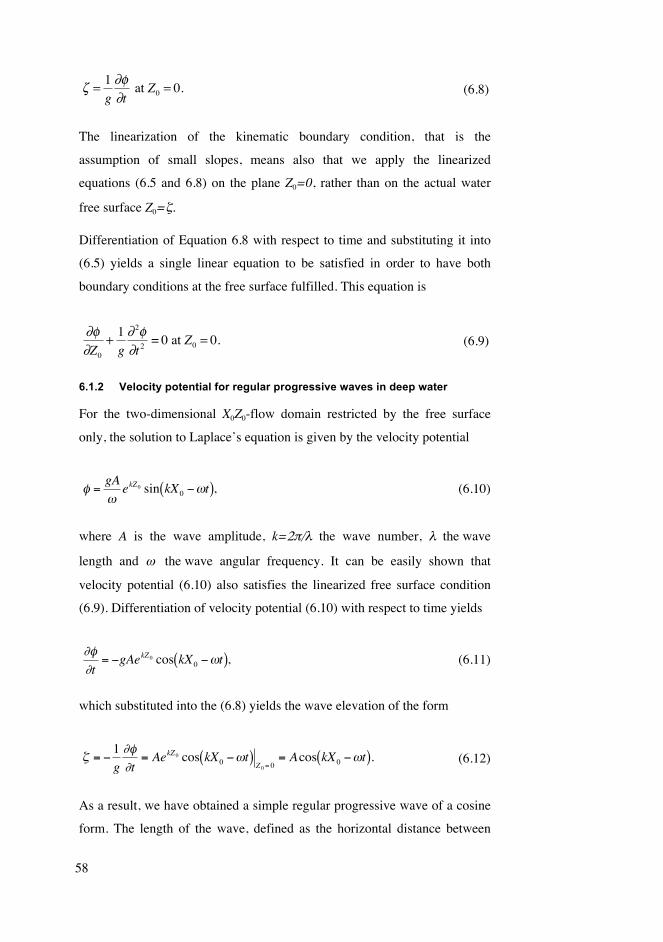
58
ζ = 1
g
∂φ∂t
at Z0 = 0.
(6.8)
The linearization of the kinematic boundary condition, that is the
assumption of small slopes, means also that we apply the linearized
equations (6.5 and 6.8) on the plane Z0=0, rather than on the actual water
free surface Z0=ζ.
Differentiation of Equation 6.8 with respect to time and substituting it into
(6.5) yields a single linear equation to be satisfied in order to have both
boundary conditions at the free surface fulfilled. This equation is
∂φ∂Z0
+ 1
g
∂ 2φ∂t 2 = 0 at Z0 = 0.
(6.9)
6.1.2 Velocity potential for regular progressive waves in deep water
For the two-dimensional X0Z0-flow domain restricted by the free surface
only, the solution to Laplace’s equation is given by the velocity potential
(6.10)
where A is the wave amplitude, k=2π/λ the wave number, λ the wave
length and ω the wave angular frequency. It can be easily shown that
velocity potential (6.10) also satisfies the linearized free surface condition
(6.9). Differentiation of velocity potential (6.10) with respect to time yields
(6.11)
which substituted into the (6.8) yields the wave elevation of the form
(6.12)
As a result, we have obtained a simple regular progressive wave of a cosine
form. The length of the wave, defined as the horizontal distance between
=gA
ekZ0 sin kX0 t( ),
t= gAekZ 0 cos kX0 t( ),
=1
g t= AekZ 0 cos kX0 t( )
Z 0= 0= Acos kX0 t( ).

59
two successive crests or troughs, is λ=2π/k. It is interesting to notice that the
cosine function applies both to the spatial (X0-directional) and to the time
dependence. Thus the spatial form of the wave is that of a cosine function,
and the time dependency of the water elevation at the fixed position X0 = Xi
is also of the same form. Quantities used in describing the regular
progressive wave are shown in Fig. 6.3 below.
Fig. 6.3 Progressive regular wave at a certain instant of time.
In Figure 6.3, Vp is the wave celerity, also called the phase velocity, and H is
the wave height.
6.1.3 Dispersion relation for the deep water
There is a relation between the wave frequency and length. This
dependence, called the dispersion relation, for the deep water is obtained
substituting (6.10) in (6.9):
∂φ∂Z0
+ 1g
∂ 2φ∂t 2
= kgA
ωekZ 0 sin kX0 −ωt( ) − AωekZ 0 sin kX0 −ωt( ) = 0
(6.13)
yielding
k = 2πλ
= ω 2
g . (6.14)
6.1.4 Fluid velocity and pressure below progressive regular waves in deep water
The flow velocities can be readily obtained from the velocity potential as
follows

60
(6.15)
The pressure can be evaluated from Bernoulli’s equation (6.6) and using the
velocity potential 6.10 as follows
(6.16)
It is quite usual to disregard the last term as a nonlinear and having little
significance. Thus the pressure in the fluid domain, that is for Z0≤0, is given
by
pt = p − pa = ρgζekZ 0 − ρgZ0 ≡ pd + ph , (6.17)
where pd is the so-called dynamic and ph the hydrostatic part of the pressure.
u0 =X0
=gAk
ekZ 0 cos kX0 t( )
w0 = Z0=gAk
ekZ 0 sin kX0 t( ).
p pa = gZ0 t
1
2•
= g AekZ0 cos kX0 t( ) Z0[ ]1
2
gAk
2
e2kZ 0 .

61
Fig. 6.4 Iso-lines of dynamic pressure due to a linear progressive wave of a
length 3 m and amplitude 0.2 m. At the upper figure the linear term (the first
bracketed term of Equation 6.16) is presented. The bottom figure includes
also the nonlinear, third term of Equation 6.16.
As is clearly seen from Figure 6.4, the nonlinear term does not have much
effect on the absolute value of the pressure, even in this very steep wave
case. Actually so a steep wave is not of a cosine form. An increase in wave
steepness is associated with the sharpening of the crests while the troughs
get flatter. Steep waves are shown in Figure 6.1. The steepest possible
waves are usually represented by a trochoid, as shown in Figure 6.5 below.

62
Fig. 6.5 Trochoidal steepest wave.
The nonlinear effects in water surface waves are further discussed in Section
6.2.
6.1.5 Wave celerity
Let us imagine an observer travelling at speed Vp along the X-axis so that its
position is given by
(6.18)
Using (6.12), the velocity of the wave surface elevation felt by the observer
is given by
∂ζ∂ t
= Ad
dtcos kXINIT + kVp −ω( )t⎡⎣ ⎤⎦
= −A kVp −ω( )sin kXINIT + kVp −ω( )t⎡⎣ ⎤⎦. (6.19)
The observer will see the wave as a stationary one if the following holds
(6.20)
which infers that the velocity of wave profile travel in deep water, the so-
called phase velocity (refer to Figure 6.3) or the wave celerity, is
(6.21)
X0 = XINIT +Vpt.
kVp −ω = 0,
Vp =ω /k.
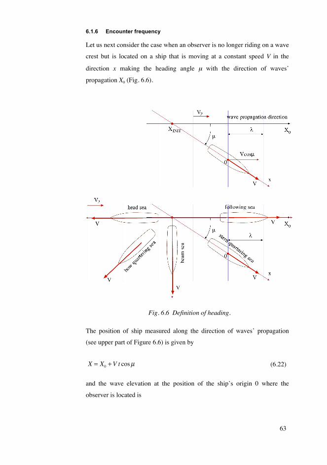
63
6.1.6 Encounter frequency
Let us next consider the case when an observer is no longer riding on a wave
crest but is located on a ship that is moving at a constant speed V in the
direction x making the heading angle μ with the direction of waves’
propagation X0 (Fig. 6.6).
Fig. 6.6 Definition of heading.
The position of ship measured along the direction of waves’ propagation
(see upper part of Figure 6.6) is given by
(6.22)
and the wave elevation at the position of the ship’s origin 0 where the
observer is located is
X = X0 +V t cosμ

64
ζ = Acos kX0 + kVt cosμ −ωt( ) = Acos kX0 − ω − kV cosμ( )t⎡⎣ ⎤⎦. (6.23)
Using (6.14) the last term in parenthesis
(6.24)
is called the frequency of encounter. It is the angular frequency the waves
are felt by the ship. Different heading angles and their definitions are given
in the lower part of Figure 6.6. From the form of expression 6.24, it is
clearly seen that:
For the head sea (μ=1800), that is heading into waves and swell, the
encounter frequency is higher than the wave frequency and the difference
increases with ship speed.
For beam seas (μ =900), heading 900 across the seas, the encounter
frequency equals the wave frequency.
For following seas (μ =00), heading with the seas, the encounter frequency is
lower than the wave frequency and the difference increases with ship speed.
The encounter frequency is zero if the ship speed projected in the direction
of wave propagation equals the wave celerity, i.e. Vcosμ=Vp. A further
decrease in ship speed or increasing wave length yields the situation where
waves propagate faster than the ship and they start to overtake it.
6.2 The effects of shallow water
Shallow water affects the free surface deformation and the creation of
surface waves. The velocity potential has to satisfy in addition to the free
surface boundary condition (6.9), also the impermeability condition at the
sea bottom:
w0 = ∂φ∂Z0
= 0 at Z0 = −h,
(6.25)
ω e =ω − kV cosγ =ω 1−Vωgcosμ
⎛⎝⎜
⎞⎠⎟
65
where h is the water depth. It can be shown that the velocity potential
satisfying these conditions is of the form
φ = gA
ωcoshk(Z0 + h)coshkh
sin kX0 −ωt( ).
(6.26)
The dispersion relation following from the satisfaction of the free surface
boundary conditions gets more complicated and is given by the expression
k tanhkh = ω 2 /g. (6.27)
The phase velocity for the limited water depth is given by
Vp = ω /k = gtanhkh
k.
(6.28)
The Taylor series expansion of hyperbolic tangent of 6.28 yields
Vp = gkh − (kh)3 /3+ ...
k (6.29)
giving an approximate expression
Vp ≈ gh (6.30)
for the phase velocity when kh = 2πh /λ <<1. In this case the phase velocity
does not depend on the wave length.
6.3 Nonlinear models of surface waves
As will be discussed in the next sections, the linear wave model is very
useful. The advantages are that it is easy to use, complies well with the
linear modelling of ship motions in waves and makes it possible to model
the sea condition consisting of waves of different lengths and heights.
However, in some cases, certain nonlinear effects have to be considered. For
instance, if we are dealing with an evaluation of local wave pressure loads
on a ship’s side shell, it is important to consider the pressures up to the
actual instantaneous water free surface. The information provided by the

66
linear wave model just up to the still water level is not sufficient. As already
mentioned, an increase in wave steepness results in wave profiles that differ
from the ideal cosine form (Figure 6.5). An elegant and efficient way of
dealing with steep regular waves is provided by the so-called Stokes’
expansion (Newman, 1977). However, this will be not discussed here
because this wave model is seldom used in ship dynamics. Moreover, it can
be found in a number of books dealing with surface waves. Instead, in the
following, we shall discuss two simplified heuristic models. Both models
retain the regular cosine form of surface wave. What distinguishes them
from the linear model is the fact that they attempt to evaluate the pressures
up to the actual water surface.
6.3.1 The Faltinsen’s model of pressure
In the model of Faltinsen (Faltinsen, 1990) both the hydrostatic and the
dynamic pressure part are calculated from the still water level being the
reference. In this sense, the method is in agreement with the linear wave
theory. For the wave crest, the dynamic pressure is extended as a uniform
distribution from the still water level up to the actual water surface (see Fig.
6.7). For a wave trough, the hydrodynamic pressure is disregarded in the
region located between the actual water surface and the still water level. As
a result, a small non-zero total pressure pt at the actual water surface is
obtained. Thus the dynamic boundary condition is not fully fulfilled for the
wave trough.

67
Fig. 6.7 Extrapolation of the hydrodynamic pressures above and below the
still water level (Faltinsen, 1990).
6.3.2 Stretching approximation of pressure distributions
The so-called stretching for the pressure distributions stems from the desire
to have the dynamic boundary condition fulfilled on the water free surface.
For the deep water condition, this technique is given by the following
formula
pt = p − pa = ρgζek Z 0−ζ( ) − ρgZ0 = pd + ph . (6.31)
Stretched pressures are presented in Fig. 6.8 below.

68
Fig. 6.8 Stretched pressure distributions.
6.4 Wave group
The concept of a wave group can be explained by considering waves
resulting from the superposition of two cosine form wave trains having the
same amplitude A but slightly different angular frequencies ω1 and ω2. The
resulting water surface elevation is
ζ = Acos k1X0 −ω1t( )+ Acos k2X0 −ω2t( )
= 2Acosk1 + k2( )X0 − ω1 +ω2( )t
2
⎡
⎣⎢
⎤
⎦⎥cos
k1 − k2( )X0 − ω1 −ω2( )t2
⎡
⎣⎢
⎤
⎦⎥
= 2Acos kmeanX0 −ωmeant( )cos δk2
X0 −δω2
t⎛
⎝⎜
⎞
⎠⎟.
(6.32)
The resulting wave is shown in Figure 6.9. It consists of the so-called carrier
frequency wave with angular frequency ωmean=(ω1+ω1)/2 and slowly varying
component with frequency δω/2=(ω1−ω2)/2.
The group velocity, which is the velocity of propagation of a group of
carrier waves, is obtained by setting the observer of the waves following the
group with the velocity Vg. The X-directional position of the observer is
given by

69
X0 = XINIT +Vgt. (6.33)
Thus,
ζ = 2Acos kmeanX0 −ωmeant( )cos δk2
XINIT +Vgt( )− δω2
t⎡
⎣⎢⎤
⎦⎥
= 2Acos kmeanX0 −ωmeant( )cos δk2XINIT+ δkVg −δω( )t / 2
⎡
⎣⎢⎤
⎦⎥.
(6.34)
Following the reasoning of frequency of encounter, the wave group velocity
in the deep water case is
Vg = δωδk
≈ dωdk
= 12
g
k= 12
ωk
= 12Vp .
(6.35)
Fig.6.9 Wave groups as the result of a superposition of two wave trains. A1=A=0.2 m and ω1= 4.53 rad/s and ω 2= 4.96 rad/s.
From (6.35) we see that in the deep water, the group velocity is half of the
phase velocity. If we conduct model tests in a tank and create the waves at
one end of the basin, the group velocity rules the time required by the waves
to arrive at the measuring position.
6.5 Spectral representations of sea surface waves
It is quite obvious that sea surface waves are far more complex than the ones
described above. What we observe is a variety of waves with different
-0.5
-0.4
-0.3
-0.2
-0.1
0
0.1
0.2
0.3
0.4
0.5
0 5 10 15 20 25 30 35 40
t [s]
[m
]

70
frequencies and different heights. Fortunately, there is a dispersion relation
giving a connection between the wave frequency and length. Moreover, the
waves propagate in different directions, although usually most of them
follow the wind direction. Thus there is a prevailing course of their motion.
This nearly unidirectional propagation of waves makes it possible to use a
simplified model of irregular waves, the so-called long-crested waves
model.
6.5.1 Long-crested irregular waves
Let us consider three regular waves propagating in the positive X0-direction
having amplitude Ai and frequency ωI (i=1,2,3). The component waves and
the resulting irregular combination of them are shown in Figure 6.10 with
the phase of each of them being selected at random.
Fig. 6.10 Irregular wave as a sum (denoted by Σ) of the three regular wave components.
Spectral representation of the wave train of Figure 6.10 is shown in Figure
6.11.
-2.5
-2
-1.5
-1
-0.5
0
0.5
1
1.5
2
2.5
0 10 20 30 40 50 60
time [s]
[m
]
1 2 3

71
Fig. 6.11 A discrete amplitude spectrum of the wave train of Figure 6.10.
In Figure 6.11, co-ordinates are the frequencies and ordinates the amplitudes
of the component waves. In order to describe wave trains comprising of an
infinite number of regular components, another type of spectral
representation is used. The so-called power spectral density is used instead
of a discrete amplitude spectrum. This is a continuous function of wave
angular frequency ω, which gives information on the wave amplitude related
to a certain frequency. An example of the wave spectrum is presented in
Figure 6.12.
Fig. 6.12 Power spectral density of wave amplitude represented by N=100
frequency components.
0
0.2
0.4
0.6
0.8
1
1.2
0.5 0.7 0.9
omega [rad/s]
A [
m]
0
0.5
1
1.5
2
2.5
3
3.5
0.4 0.6 1 1.2 1.4 1.6 1.8 2
S(ω)
ω [rad/s]
[m^2 s]
Δω
S(ω) Δω
ω0

72
The area under the curve represented by dots is a measure of the energy
density of water surface motion. This energy given by
E = ρg S ω( )0
∞
∫ dω =ρg2N
Ai2 = ρgσ 2
1
N
∑ ,
(6.36)
where σ2 is variance of the wave signal. An amplitude of a single wave
component having the angular frequency ωi can be evaluated by the
integration of the wave spectrum as follows:
Ai = 2S ωi( )Δω .
(6.37)
Note that frequency differential Δω can be selected freely. Quite often, in
order to secure a generation of non-repeatable wave trains from the given
wave spectrum, the sample angular frequencies ωi are random numbers
covering the frequency range of interest (ωmin≤ ω ≤ωmax). In this case, the
frequency increments Δωi are also random numbers governed by the
adjacent frequencies ωi and ωi+1. The wave train from the given wave
spectrum is obtained as
ζ (t)= ai sinωit +bi cosωit =i=1
N
∑ Ai cos ωit −δi( )i=1
N
∑ ,
(6.38)
where −π≤δi≤π is a random number representing the phase angle of the ith
wave component. Wave elevation given by formula (6.38) can be
understood as measured at the origin of the co-ordinate system, that is X0=0.
This wave generation is based on the so-called Deterministic Spectral
Amplitude model. In the so-called Non-deterministic Spectral Amplitude
model the ai and bi coefficients of the series (6.38) are taken as a normally
distributed uncorrelated variables (Naito, 1995). This results in the wave
amplitude component evaluated with the aid of (Matusiak, 2000)
Ai = 2S ωi( ) χ22
2Δω ,
(6.39)

73
where χ22 is a chi-squared distribution with two degrees of freedom that
results from the normal distribution of ai and bi coefficients. Randomness of
wave amplitudes is observed in nature. If we took a number of relatively
short records of waves at sea, we should notice that the power spectrum
based on each of them is very irregular and different at each time. The
common feature would be the area made up by each spectrum, which is
nearly the same. The ensemble average of these spectra yields the smoothed
wave spectrum as the one in Figure 6.12. This smoothed spectrum can be
also understood as the spectrum obtained by processing a very long time
record.
Other parameters describing in general terms the wave spectra are spectrum
moments and periods. The kth moment of spectrum is evaluated by the
following form integral
mk = ω k
0
∞
∫ S ω( )dω.
(6.40)
The so-called significant wave height is defined by
HS = 4 m0 . (6.40a)
Another symbol frequently used for the significant wave height is H1/3. This
stems from the fact that the significant wave height is the mean of one-third
of the highest observed waves. As a rule of thumb we can take that the
highest wave encountered at sea is approximately twice the significant wave
height. The latter number is roughly what is observed visually as the wave
height.
There are many wave spectra used to describe wave conditions at sea. In
seakeeping the most often used is the spectrum recommended by the ISSC
(International Ship and Offshore Structures Congress) and the so-called
Jonswap wave spectrum. The ISSC (two-parameter) wave spectrum is
appropriate to describe developed ocean waves; it is given by

74
S(ω)=171.44H1/3
2
T14ω 5
exp−685.76
T14ω 4
⎛
⎝⎜
⎞
⎠⎟ [m2s],
(6.41)
where T1 is the average wave period. T1 is related to the spectral moments by
T1 = 2πm0 /m1. (6.42)
The Jonswap spectrum can be evaluated either from the significant wave
height and from the average period or from wind velocity U and fetch X. In
the first case, the spectrum is given by
S(ω)=155H1/3
2
T14ω 5
exp−944
T14ω 4
⎛
⎝⎜
⎞
⎠⎟(3.3)γ [m2s],
(6.43)
where
γ = exp − ω /ω0 −12σ
⎛ ⎝ ⎜
⎞ ⎠ ⎟ 2⎡
⎣ ⎢ ⎢
⎤
⎦ ⎥ ⎥
(6.44)
and
σ = 0.07 for ω ≤ 5.24T1
σ = 0.09 for ω > 5.24T1.
In the second case, the Jonswap spectrum is given by
S(ω)=αg2
ω 5exp −
5
4
ω0
ω
⎛
⎝⎜
⎞
⎠⎟
4⎡
⎣⎢⎢
⎤
⎦⎥⎥(3.3)γ [m2s],
(6.45)
where the so-called Philip’s number is
α = 0.076gX
U 2
⎛
⎝⎜
⎞
⎠⎟−0.22
,
(6.46)

75
with U [m/s] and X [m] being the wind velocity and fetch respectively. Fetch
means the sea distance over which wind blows. The so-called modal angular
frequency is denoted by ω0 and given by the relation
ω0 = 7πg
U
gX
U 2
⎛
⎝⎜
⎞
⎠⎟−0.33
.
(6.47)
This frequency is related to the modal period by the expression ω0=2π/T0
For the Jonswap spectrum, the following relation for the spectral periods
holds (Faltinsen, 1990)
T1 = 0.834T0. (6.48)
Both wave spectra are presented in Figure 6.13.
Fig. 6.13 ISSC and Jonswap wave spectra. T1=7.5 [s] and HS=4.5 [m].
As can be seen from the spectra comparison, the frequency content of
Jonswap spectrum is more concentrated and located more towards higher
frequencies, i.e. shorter waves. This means that this spectrum is usually
better suited for a raising storm and for a limited fetch than the other one.
0
1
2
3
4
5
6
0.25 0.5 0.75 1 1.25 1.5 [rad/s]
S [m
^2 s
]
ISSCJonswap

76
6.5.2 Short-crested irregular waves
An extension of Fourier representation (6.38) of surface waves allowing for
wave propagation at angle μ with respect to axis X of the co-ordinate system
fixed with Earth of the form
ζ (X0,Y0;t) = Ai cos ki X0 cosμi +Y0 sinμi( ) −ω it + δi[ ]i=1
N
∑
(6.49)
can in principle be used. Similarly as for the long-crested waves, a spectral
representation of directional spectrum S(ω,μ) can be derived such that
σ 2 = S ω,μ( )0
∞
∫ dωdμ0
2π
∫ .
(6.50)
The feature of multi-directional wave propagation, if at all taken into
account, is modelled by introducing the so-called spreading function f(μ)
such that the directional spectrum is presented as a product of two functions
S ω,μ( ) = S ω( ) f (μ). (6.51)
ITTC recommends a spreading function of the form
f (μ) = 2
πcos2 μ, where −π /2 < μ < π /2.
(6.52)

77
7. Hydrodynamic forces acting on a rigid body in waves
7.1 Velocity potential due to ship oscillatory motion and caused by wave action
We assume that the flow associated with the motion of a ship hull in waves
is well represented by the potential flow approximation. That is, we
disregard the viscous effects. A ship is a rigid body moving in six degrees of
freedom. The action of regular sinusoidal form waves of frequency ω is felt
by a moving ship as the oscillatory excitation with the encounter frequency
ωe. We disregard initial transients and assume linearity of the ship’s
response to wave action. This motion in the j-th degree of freedom is
denoted by ξj and it is given by the formula
ξ j (x, y, z,t)=ξ0 jeiωet ,
(7.1)
where ξ0j is the complex amplitude of the j-th displacement component. Note
that for the sake of convenience, we use exponential function notation rather
than trigonometric functions for representing the oscillatory motion. The
real part of (7.1) can be taken in order to have an instantaneous value of
displacement.
Moreover, at least at the beginning, we assume that the amplitudes ξ0j of this
oscillatory motion are small. This assumption means that the waves
affecting ship are of small amplitude, too. Another important fact resulting
from the small amplitude assumption is that we do not have to take into
account complicated relations (3.4) and (3.6) between the inertial and body-
fixed coordinate systems when describing ship motions.

78
This means that the following simplified relations hold:
˙ ξ 1 = u = ˙ X G , ˙ ξ 2 = v = ˙ Y G, ˙ ξ 3 = w = ˙ Z G, ˙ ξ 4 = p, ˙ ξ 5 = q, ˙ ξ 6 = r. (7.2)
The assumption of linearity substantially simplifies equations of motion
(4.4) and (4.7).
Velocity of any point P of the body can be presented in the following form
V = V0 + Ω× r , (7.3)
where V0 is the velocity of the origin, ΩΩ=pi+qj+rk is the angular velocity,
and r is the position vector of point P. The velocity normal to the body
surface is given by
vn = V0 •n+ Ω× r( ) •n = V0 •n+ Ω• r ×n( )= ˙ ξ 1n1 + ˙ ξ 2n2 + ˙ ξ 3n3 + ˙ ξ 4 r ×n( )1
+ ˙ ξ 5 r ×n( )2+ ˙ ξ 6 r ×n( )3
= ˙ ξ jn j
j=1
3
∑ + ˙ ξ j r ×n( ) j−3j= 4
6
∑ ,
(7.4)
where n is the unit normal to the body surface directed into the body and nj
is projection of it in the j-th direction.
As the motion is oscillatory, with constant amplitude, this means that we
disregard the transients and concentrate on the fully developed responses
caused by regular linear waves, such as the ones given by formula (6.12) or
(6.23). The small amplitude assumption makes it possible to use the benefits
of the model’s linearity. The biggest advantage is in using the superposition
principle. This allows us to construct the total flow model and the ship
response to waves as the sums of simple sub-models. Thus, for instance, the
responses in irregular sea waves can be easily computed using the spectral
representation of surface waves presented in Section 6.5.
A linearity assumption makes it also possible to present the total flow due to
the ship oscillatory motion and caused by waves as a sum of velocity
potentials

79
φ(x, y, z,t)=Re ξ0 jφ j (x, y, z)+ AφA(x, y, z)j=1
6
∑⎡
⎣⎢⎢
⎤
⎦⎥⎥eiωet
⎧⎨⎪
⎩⎪
⎫⎬⎪
⎭⎪.
(7.5)
The flow disturbance produced by a ship’s motion in still water is
represented by the first term (sum-term) in the brackets. An oscillatory
motion of a ship in the j-th degree of freedom with unit amplitude is
represented by the velocity potential φj. The action of waves is represented
by the second term in the brackets. This term comprises the amplitude of the
velocity potential of an oncoming wave having an amplitude of 1 m (see Eq.
6.10) and denoted in the following by φ0, and the amplitude of the so-called
diffraction potential φ7. The latter takes into account the disturbance effect
of the ship on the oncoming wave. Thus the amplitude of the velocity
potential describing the action of a wave having amplitude equal to 1 m can
be written as the sum of both potentials:
φA = φ0 +φ7. (7.6)
7.2 Boundary conditions
The boundary conditions for the oncoming waves were dealt with in Section
6.1. The boundary condition for the diffraction velocity potential stems from
the fact that there is no flow through the hull surface SB. This means that the
normal velocity component of flow due to oncoming waves and that of the
diffracted waves must be of the same magnitudes but of the opposite sign,
that is
∂φ7∂n
= −∂φ0∂n
(7.7)
at the body surface SB. This is equivalent to the requirement that the normal
component of the total to hull flow velocity due to waves is zero that is
∂φA∂n
= 0. (7.8)
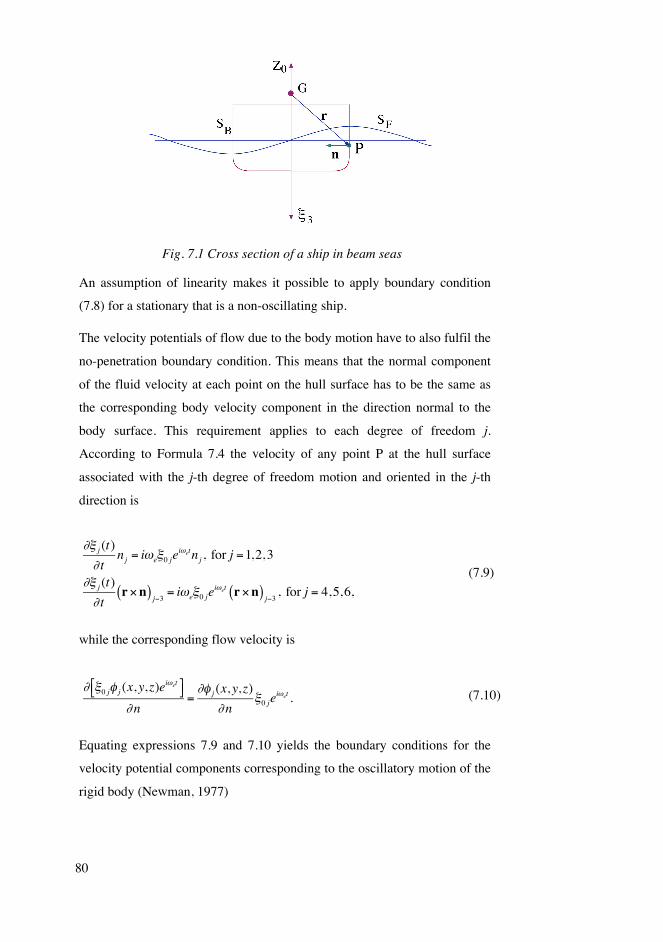
80
Fig. 7.1 Cross section of a ship in beam seas
An assumption of linearity makes it possible to apply boundary condition
(7.8) for a stationary that is a non-oscillating ship.
The velocity potentials of flow due to the body motion have to also fulfil the
no-penetration boundary condition. This means that the normal component
of the fluid velocity at each point on the hull surface has to be the same as
the corresponding body velocity component in the direction normal to the
body surface. This requirement applies to each degree of freedom j.
According to Formula 7.4 the velocity of any point P at the hull surface
associated with the j-th degree of freedom motion and oriented in the j-th
direction is
∂ξ j (t)
∂ tnj = iωeξ0 je
iωetn j , for j =1,2,3
∂ξ j (t)
∂ tr×n( ) j−3
= iωeξ0 jeiωet r×n( ) j−3
, for j = 4,5,6,
(7.9)
while the corresponding flow velocity is
∂ ξ0 jφ j (x, y, z)eiωet⎡⎣ ⎤⎦
∂n=∂φ j (x, y, z)
∂nξ0 je
iωet .
(7.10)
Equating expressions 7.9 and 7.10 yields the boundary conditions for the
velocity potential components corresponding to the oscillatory motion of the
rigid body (Newman, 1977)

81
∂φ j
∂n= iωen j , for j = 1,2,3
∂φ j
∂n= iωe r ×n( ) j−3
, for j = 4,5,6.
(7.11)
7.3 Linear hydrodynamic forces in general
Hydrodynamic forces acting on a ship’s hull can be evaluated using
Bernoulli’s equation
ρ∂φ∂t
− ρgZ1 + 12ρ v 2 + p = C,
(7.12)
where Z1 is the vertical distance measured from the still water level
downwards. Using the velocity potential (7.5) and retaining in Bernoulli’s
equation only the linear terms, the following expression for the total
pressure is obtained
p = −ρ∂φ∂ t
+ ρgZ1 = −ρRe ξ0 jφ j (x, y, z)+ A φ0 +φ7( )j=1
6
∑⎡
⎣⎢⎢
⎤
⎦⎥⎥iωee
iωet⎧⎨⎪
⎩⎪
⎫⎬⎪
⎭⎪+ ρgZ1.
(7.13)
The total force F and moment M due to this pressure are obtained by
FM
⎛
⎝⎜
⎞
⎠⎟=
pn
p r×n( )
⎛
⎝
⎜⎜
⎞
⎠
⎟⎟
S
∫ dS = ρg nr×n
⎛
⎝⎜
⎞
⎠⎟
S
∫ Z1dS
−ρRe iωeξ0 jeiωet n
r×n
⎛
⎝⎜
⎞
⎠⎟
S
∫ φ jdSj=1
6
∑⎡
⎣⎢⎢
⎤
⎦⎥⎥− ρRe iωeAe
iωet nr×n
⎛
⎝⎜
⎞
⎠⎟
S
∫ φ0 +φ7( )dS⎡
⎣⎢⎢
⎤
⎦⎥⎥,
(7.14)
where integrals are taken over the wetted surface of the hull. Using the
boundary conditions 7.11, the k=1,2,3 component of force or moment (with
k=4,5,6 for x,y and z-directional component respectively) can be presented
as

82
Fk = ρgnk
r ×n( )k−3⎛
⎝ ⎜
⎞
⎠ ⎟
S
∫ Z1dS − ρRe ξ0 jeiω e t
∂φk∂nS
∫ φ jdSj=1
6
∑⎡
⎣ ⎢ ⎢
⎤
⎦⎥⎥
−ρARe eiω e t∂φk∂nS
∫ φ0 + φ7( )dS⎡
⎣ ⎢
⎤
⎦ ⎥ .
(7.15)
The first term in (7.15) depicts the hydrostatic load. The second term
describes the radiation forces while the third term represents the wave
loading. The name radiation forces stems from the fact that these are the
fluid reaction forces to the oscillatory motion with a finite acceleration.
Radiation and wave forces are solved separately and they are evaluated for a
ship moving steadily without wave-induced motions being taken into
account. In other words, wetted surface S does not change.
7.4 Hydrostatic forces
Hydrostatic forces and moments depict the reactions of water acting in calm
water on a hull subjected to a very slow motion. Note that these forces are
dependent on the geometry of only the submerged part of the hull. As the
hydrostatics were covered in the Ship Buoyancy and Stability course, only a
brief summary is presented in the following of what was dealt with earlier.
Instead, we shall elaborate on a three-dimensional model of evaluating the
nonlinear hydrostatic loads.
7.4.1 Linear approximation
In case of the hydrostatic forces, a linearity assumption means that they are
dealt with using the initial stability model. This model yields a linear
relation between hull slow sinkage zL, heel φL and trim θL motions and the
corresponding restoring vertical force Zrestoring,L and two corresponding
moments Krestoring,L and Mrestoring,L. These relations are:
Zrestoring,L = −ρgAWzL + ρgAWxFθLKrestoring,L = −mgGMTφLMrestoring,L = ρgAWxFzL −mgGMLθL ,
(7.16)
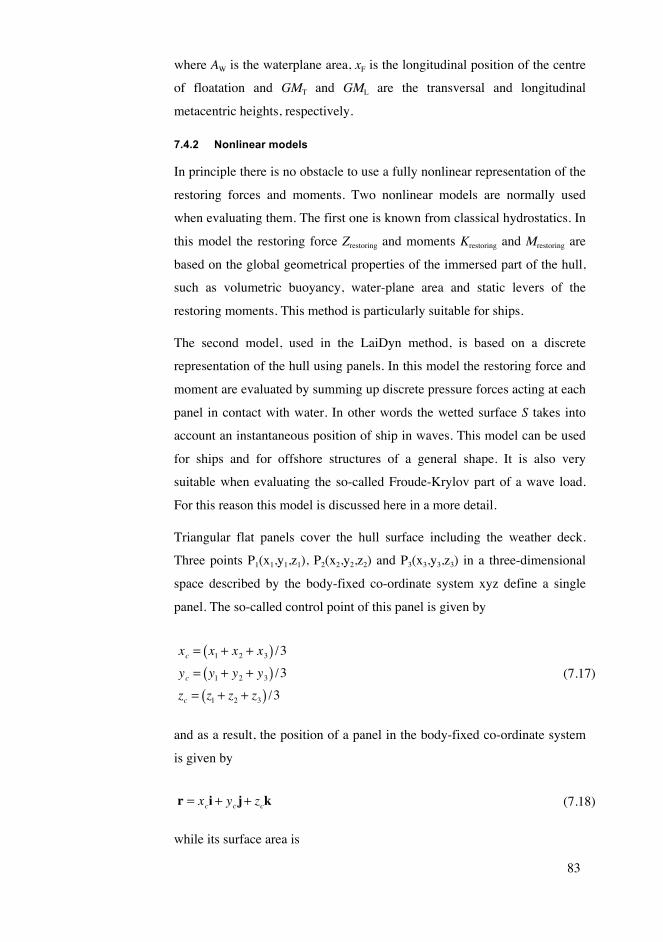
83
where AW is the waterplane area, xF is the longitudinal position of the centre
of floatation and GMT and GML are the transversal and longitudinal
metacentric heights, respectively.
7.4.2 Nonlinear models
In principle there is no obstacle to use a fully nonlinear representation of the
restoring forces and moments. Two nonlinear models are normally used
when evaluating them. The first one is known from classical hydrostatics. In
this model the restoring force Zrestoring and moments Krestoring and Mrestoring are
based on the global geometrical properties of the immersed part of the hull,
such as volumetric buoyancy, water-plane area and static levers of the
restoring moments. This method is particularly suitable for ships.
The second model, used in the LaiDyn method, is based on a discrete
representation of the hull using panels. In this model the restoring force and
moment are evaluated by summing up discrete pressure forces acting at each
panel in contact with water. In other words the wetted surface S takes into
account an instantaneous position of ship in waves. This model can be used
for ships and for offshore structures of a general shape. It is also very
suitable when evaluating the so-called Froude-Krylov part of a wave load.
For this reason this model is discussed here in a more detail.
Triangular flat panels cover the hull surface including the weather deck.
Three points P1(x1,y1,z1), P2(x2,y2,z2) and P3(x3,y3,z3) in a three-dimensional
space described by the body-fixed co-ordinate system xyz define a single
panel. The so-called control point of this panel is given by
xc = x1 + x2 + x3( ) /3yc = y1 + y2 + y3( ) /3zc = z1 + z2 + z3( ) /3
(7.17)
and as a result, the position of a panel in the body-fixed co-ordinate system
is given by
r = xci + yc j+ zck (7.18)
while its surface area is

84
. (7.19)
Components of the normal vector at the control point can be evaluated from
the following expressions derived from the definition of the vector product
c = a×b =
i j k
ax ay az
bx by bz
,
(7.20)
where
a = axi + ay j+ azk = (x1 − x3)i + (y1 − y3)j+ (z1 − z3)kb = bxi + by j+ bzk = (x2 − x3)i + (y2 − y3)j+ (z2 − z3)k.
(7.21)
The normal to the panel is given by
n = c/ c . (7.22)
Note that two co-ordinate systems are used when evaluating the hydrostatic
loads. The position of the panel (given by the co-ordinates of its control
point) and the components of the normal vector n are given in the body-
fixed co-ordinate system (xyz of Fig. 1). The depth Zc of each control point
is measured in the global inertial co-ordinate system (XYZ in figures 3.1 and
7.2). The following relation, being derived from expression (3.4), can be
used when transforming the control or other ship’s points (xc,yc,zc) from the
moving body-fixed co-ordinate system to the Earth-fixed inertial system
Xc
YcZc
⎧ ⎨ ⎪
⎩ ⎪
⎫ ⎬ ⎪
⎭ ⎪ =
δXG
δYGδZG
⎧ ⎨ ⎪
⎩ ⎪
⎫ ⎬ ⎪
⎭ ⎪ +
cosψ cosθcosψ sinθ sinφ−sinψ cosφ
cosψ sinθ cosφ+ sinψ sinφ
sinψ cosθsinψ sinθ sinφ+cosψ cosφ
sinψ sinθ cosφ−cosψ sinφ
−sinθ cosθ sinφ cosθ cosφ
⎡
⎣
⎢ ⎢ ⎢ ⎢ ⎢ ⎢
⎤
⎦
⎥ ⎥ ⎥ ⎥ ⎥ ⎥
xcyczc
⎧ ⎨ ⎪
⎩ ⎪
⎫ ⎬ ⎪
⎭ ⎪ .
(7.23)
ΔS = 12
y1 z1 1
y2 z2 1
y3 z3 1
2
+z1 x1 1
z2 x2 1
z3 x3 1
2
+x1 y1 1
x2 y2 1
x3 y3 1
2
85
In the above formula, δXG, δYG and δZG are surge, sway and heave
displacements of the ship’s centre of gravity G. Using the Formula 7.23, the
one can evaluate the depth Zc of any panel of a rigid ship having 6 degrees-
of-freedom motion as follows
Zc =δZG − xc sinθ+ yc cosθ sinφ+ zc cosθ cosφ. (7.24)
As could be expected, the panel’s depth does not depend on surge, sway and
yaw motions.
7.5 Nonlinear hydrostatic and Froude-Krylov forces
The Froude-Krylov pressures are the pressures in an undisturbed surface
wave. For a linear (the so-called Airy) wave, this pressure is given by
Expression 6.17. Moreover, the linearity assumption of the Froude-Krylov
forces means that they are evaluated for a ship without taking into account
wave-induced motions. Thus the pressure is evaluated at the stationary (non-
oscillating) hull location without taking the disturbances to the waves
caused by the ship into account. If we want to take into account the
nonlinearities of the hydrostatic and Froude-Krylov forces we can integrate
the pressure (6.17) or (6.31) given by
p = ρg ζe−k Zc +ζ( ) + Zc⎡⎣ ⎤⎦
(7.25)
over the instantaneous wetted surface S with Zc given by 7.24 and for an
instantaneous hull position. This is illustrated in Figure 7.2.

86
Fig. 7.2 Hydrostatic and Froude-Krylov pressure.
Wave elevation is given by
ζ t( ) = − 1g
∂φ0∂ t z1=0
= Acos k Xc cosμ −Yc sinμ( )−ωt⎡⎣ ⎤⎦,
(7.26)
where φ0 is the velocity potential of an oncoming wave given by (6.10), Xc
and Yc are the control points of the hull surface given in the Earth-fixed co-
ordinate system XYZ evaluated with the aid of a transformation (7.23). This
transformation and evaluation of wave height is illustrated in Figure 7.3
below.
Fig. 7.3 Evaluation of wave height for a control point c.

87
The force F and moment M are obtained by integrating the pressure (7.24)
in the body fixed co-ordinate system. This integration is performed
numerically by summing up the contribution from each wetted panel using
FF.Ktotal = FF.K;i
total =i
N
∑ piΔSinii
N
∑
MF.Ktotal = ri ×FF.K;i
total ,i
N
∑
(7.27)
where N is the wetted panel number, ΔSi is the panel area, ni is the unit
vector normal to panel and ri is the position vector of the control point in the
body fixed co-ordinate system xyz.
7.6 Radiation forces
The second term in (7.15) depicts the so-called radiation forces. As already
stated, these are the forces acting on an oscillating body in still water. The k-
th component of this force (moment for k=4,5,6) can be written as
(Newman, 1980)
Frad,k = −ρRe ξ0 jeiωet ∂φk
∂nS
∫ φ jdSj=1
6
∑⎡
⎣⎢⎢
⎤
⎦⎥⎥= Re ξ0 je
iωet fkjj=1
6
∑⎡
⎣⎢⎢
⎤
⎦⎥⎥ ,
(7.28)
where
fkj = −ρ ∂φk∂nS
∫ φ jdS = −ρ φ jnkS∫ dS
(7.29)
is a complex force in the k-th direction, due to a sinusoidal motion of unit
amplitude in the direction j. In the unbounded liquid, radiation forces are the
forces related to the acceleration of small amplitude oscillations with
angular frequency ω. For the oscillations in the liquid bounded by a free
surface, radiation force is not in-phase with acceleration only. It is a
complex quantity, which is customarily presented as
fkj = ω 2akj − iωbkj (7.30)

88
with akj and bkj being the so-called added mass and damping coefficients,
respectively. The k-th component of the radiation force can be expressed in
terms of the added mass and damping coefficients as follows:
Frad ,k = − akjU j +bkjU j( )
j=1
6
∑ ,
(7.31)
where Uj and ˙ U j are velocity and acceleration of the oscillatory motion with
the j-th motion component. It can be shown (Newman, 1980) that for a body
in an unsteady motion and in an unbounded in-viscid fluid, radiation force is
in-phase with the body’s acceleration. In other words, the damping terms bkj
are zero. Moreover, the added mass coefficients are constant and they are
dependent only on the body geometry.
Using the added mass definition 7.29 and applying the free surface
boundary condition 6.9 to the velocity potential φj yields the conclusion that
in the presence of a free surface, added mass and damping coefficients are
dependent upon the angular frequency of the oscillatory motion. This
dependency and the existence of the added damping stems from the free
surface. There is a direct relation between damping and the amplitude of
waves generated by the oscillating body (Newman, 1980). Thus the
damping term can be attributed to wave-making due to the oscillatory
motion of a body in the presence of a free surface. Newman (1980) also
presents proof that both the added mass and damping coefficients are
symmetrical so that
akj = a jk and bkj = b jk . (7.32)
The details of evaluating the coefficients of added mass and damping are
given by Newman (1980), Ohkusu (1996) and Lloyd (1989), among others.
Added mass and damping coefficients are usually evaluated using a co-
ordinate system with the origin located at the water-plane. The equations of
motion are normally derived with the origin located in the centre of gravity.
For this reason, the coefficients obtained have to be transferred to the body-

89
fixed co-ordinate system x,y,z. This transformation is presented in Appendix
A.
7.6.1 Radiation forces and nonlinear models of ship dynamics
Added mass and damping terms (7.30) are normally derived for a small
amplitude oscillatory motion. This means that their use is in principle
restricted to the linear model of ship dynamics, where the wetted surface of
the hull is constant and does not change in time. Moreover, this model of
radiation forces is good for monochromatic oscillatory ship motion that is
sinusoidal motion with a single frequency. The latter restriction is relaxed
with the use of the so-called retardation function dealt with in the next
section. There are two linear approximate approaches of defining the
radiation forces in the nonlinear models of ship dynamics. The one, used in
the following, is based on the assumption that the linear radiation forces are
fixed with a ship hull. This is illustrated in Figure 7.4a. Another approach is
to assume that they are primarily ruled by the free surface and thus their
orientation is given by the inertial Earth-fixed co-ordinate system, Figure
7.4b.
Fig. 7.4 Two definitions of radiation forces orientation.
7.6.2 Memory effect of the radiation forces
In the time domain simulations radiation forces have to take into account the
history of the previous motion. The time domain approach requires the so-
called convolution integral representation of the radiation forces (Cummins,

90
1962; Johansson, 1986). In this time-domain approach radiation forces
vector Xrad is represented by the expression:
Xrad (t)= −a∞x(t)− k
−∞
t
∫ t −τ( )x(τ )dτ ,
(7.33)
where a∞ is the matrix comprising the added mass coefficients for an infinite
frequency and x is the response vector. Matrix function k is the so-called
retardation function, which takes into account the memory effect of the
radiation forces. This function can be evaluated as:
k(t)=2
πb(ω)cos(ωt)dω
0
∞
∫ ,
(7.34)
where b is the frequency dependent added damping matrix. The k(t)
functions have to be evaluated before the simulation. The Fast Fourier
Transform algorithm can be used when evaluating the retardation functions.
The procedure is described in Appendix B.
7.7 Diffraction forces
The k-th component of the diffraction force is a second part of the wave
loading given by
FWave,k = −ρARe eiω e t∂φk∂nS
∫ φ0 + φ7( )dS⎡
⎣ ⎢
⎤
⎦ ⎥ .
(7.35)
The no-penetration boundary condition at the hull surface S implies that the
following holds:
∂ φ0 + φ7( )∂n
= 0,
(7.36)
that is

91
∂φ7∂n
= −∂φ0∂n
(7.37)
at the hull surface.
The knowledge of the wave potential φ0 and condition 7.36 makes it
possible to evaluate the diffraction potential in a similar way as the potential
of the radiation problem.
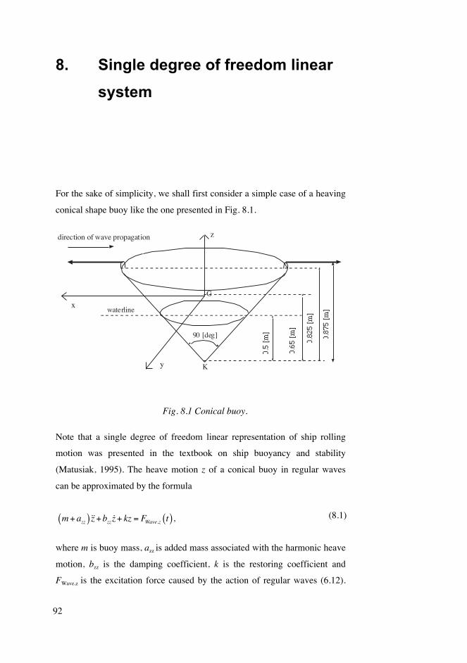
92
8. Single degree of freedom linear
system
For the sake of simplicity, we shall first consider a simple case of a heaving
conical shape buoy like the one presented in Fig. 8.1.
Fig. 8.1 Conical buoy.
Note that a single degree of freedom linear representation of ship rolling
motion was presented in the textbook on ship buoyancy and stability
(Matusiak, 1995). The heave motion z of a conical buoy in regular waves
can be approximated by the formula
m+azz( ) z+bzzz+ kz = FWave,z t( ), (8.1)
where m is buoy mass, azz is added mass associated with the harmonic heave
motion, bzz is the damping coefficient, k is the restoring coefficient and
FWave,z is the excitation force caused by the action of regular waves (6.12).
direction of wave propagation
G
waterline
K
90 [deg]
x
y
z

93
Note that both the added mass and damping coefficients depend upon the
motion frequency ω. Coefficients azz and bzz (added mass and damping)
represent the radiation force acting on a buoy in a heaving harmonic motion.
Coefficients azz and bzz are presented in Figure 8.2 below in a non-
dimensional form as azz / (ρD3) and bzz / (ρD
3ω ) , where D is a diameter of
the water-plane area.
Fig. 8.2 Non-dimensional coefficients of added mass and damping of a
conical buoy as a function of non-dimensional wave number kD.
These coefficients were obtained using the three-dimensional diffraction
problem solving method of Garrison (1974).
In Equation 8.1, the first term on the left side depicts the inertia force of the
heaving buoy, including the added mass of water following this motion. The
second term describes the damping force associated with this motion. This is
mainly caused by the wave-making effect of the heaving motion. The third
term is the restoring force known from the hydrostatics i.e. k=ρgAW, where
AW is the water-plane area (refer to Eq. 7.16). Thus the left side of Equation
8.1 represents the forces acting on the heaving buoy without taking into
account the wave effect. In other words the water surface remains still (flat).
Linearity assumption implies small amplitude motion. This makes it
possible to assume that coefficients azz and bzz are constant for harmonic
motion with a fixed frequency ω. The action of waves is represented by the
right side of Equation (8.1). The linear model of it means that it is linearly
00.250.5
0.751
1.251.5
1.752
0 2.5 5 7.5 10 12.5 15
kD
added mass added damping

94
related to the wave amplitude A (refer to sections 7.6 and 7.7) and that it can
be evaluated for a stationary buoy in a water domain limited by the still
water level.
The natural angular frequency and damping ratio of the Single-Degree-Of-
Freedom system 8.1 are given by
ωz = k / m + azz( ) (8.2)
and
ξz =bzz
2ωz m+azz( ).
(8.3)
8.1 Outline of the solution method
The solution of Equation 8.1 is normally sought in the frequency domain.
This means that the solution is derived for a number of discrete frequency
values covering a relevant range of waves’ lengths. The linearity of the
model makes it possible to seek solution for the waves of unit amplitude.
8.1.1 Hydrodynamic problem
For floating bodies possessing a general three-dimensional form there are no
simple closed form solutions for added masses, damping coefficients and
diffraction forces. However, there are numerical methods, based on panel
discretization of the body surface and on a special Green function fulfilling
the free surface conditions, capable of solving the problem stated by
equations 7.28 and 7.36 (Ohkusu, 1996; Garrison, 1974). The solution is
sought for a single frequency at a time. Usually these methods do not allow
for a forward speed of a body, and thus they are not fully capable of solving
the problem of ship hydrodynamics in waves.
8.1.2 Heave response of a buoy in waves of unit amplitude
The linear wave excitation model yields the right hand side of equation 8.1
of the form

95
FWave,z t( )m+azz
=FWave,z0
m+azzcos(ωt +δ).
(8.4)
where FWave,z0 is the amplitude of the wave force and δ is the phase angle
referred to the situation where a wave crest is passing the origin G in Fig.
8.1.
For a lightly damped case (ξz<1), Equation 8.1 has a particular solution of
the form (Kreyszig, 1993)
z(t)
A=
FWave,z0 / A
m+azz( )2 ωz2 −ω 2( )2 +bz2ω 2
cos(ωt +δ −ε),
(8.5)
where ε is the phase angle of the response referred to the wave excitation
force given by
ε = arctanωbz
m+az( ) ωz2 −ω 2( )
.
(8.6)
Taking the particular solution 8.5 as the only response component implies
that the transients due to the initial conditions have died out and the
response has achieved a steady state. Moreover, the linearity of Equation 8.1
is assumed. The form of response 8.5 as related to wave amplitude A is a
very convenient non-dimensional form making it possible to use a very
efficient and useful concept of transfer function.
The form 8.5 of response z suggests that for a wave of unit amplitude,
response amplitude is dependent upon the frequency of wave excitation
only. In other words Eq. 8.5 can be written as
z(t)
A=z0A(ω)cos(ωt +δ −ε) =
z0A(ω)cos(ωt +γ ),
(8.7)
where
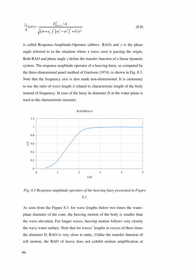
96
z0A(ω)=
FWave,z0 / A
m+azz( )2 ωz2 −ω 2( )2 +bz2ω 2
(8.8)
is called Response-Amplitude-Operator (abbrev. RAO) and γ is the phase
angle referred to in the situation where a wave crest is passing the origin.
Both RAO and phase angle γ define the transfer function of a linear dynamic
system. The response amplitude operator of a heaving buoy, as computed by
the three-dimensional panel method of Garrison (1974), is shown in Fig. 8.3.
Note that the frequency axis is also made non-dimensional. It is customary
to use the ratio of wave length λ related to characteristic length of the body
instead of frequency. In case of the buoy its diameter D at the water-plane is
used as the characteristic measure.
Fig. 8.3 Response amplitude operator of the heaving buoy presented in Figure
8.1.
As seen from the Figure 8.3, for wave lengths below two times the water-
plane diameter of the cone, the heaving motion of the body is smaller than
the wave elevation. For longer waves, heaving motion follows very closely
the wavy water surface. Note that for waves’ lengths in excess of three times
the diameter D, RAO is very close to unity. Unlike the transfer function of
roll motion, the RAO of heave does not exhibit motion amplification at
RAO(Heave)
0
0,2
0,4
0,6
0,8
1
1,2
0 1 2 3 4 5
/D
z/A

97
resonance. This is mainly due to a substantial damping associated with
wave-making caused by a heaving body. The non-dimensional form of
presentation allows a fast evaluation of the scale-free responses both for
model- and full-scale. For instance, a buoy with a water-plane diameter of
10 m in a wave of 10 m in length and 0.5 m amplitude will have a heaving
motion of 0.1 m amplitude.

98
9. Linear approximation to ship
motion in waves
A linear approximation of a ship motion in waves disregards all the
nonlinear terms of the general equations of motion (4.4) and (4.7). With this
simplification, the equations of motion are of the form
mu = Xmv = Ymw = Z
Ix p − Ixyq − Ixzr = KIyq − Iyx p − Iyzr = MIzr − Izx p − Izyq = N .
(9.1)
The left-hand sides of Equations 9.1 represent inertia forces and moments of
a ship without the contribution of added masses. The right-hand sides of the
equations 9.1 are comprised of the restoring, radiation and wave excitation
(Froude-Krylov and diffraction) forces. These are also simplified in the
linear models given in paragraph 7.4.1 and sub-chapters 7.6 and 7.7.
Equation of surge motion component, that is x-directional equation, does not
include hull resistance or propeller. Usually the forward speed of the vessel
is assumed to be nearly constant with small oscillatory variations caused by
the wave action. Harmonic surge motion, as well as other motion
components, occurs with the encounter frequency.
Linearization of the equations precludes simulation of ship manoeuvring.
The equations 9.1 are very suitable to evaluate linear, that is small
amplitude, motions in not too steep waves.
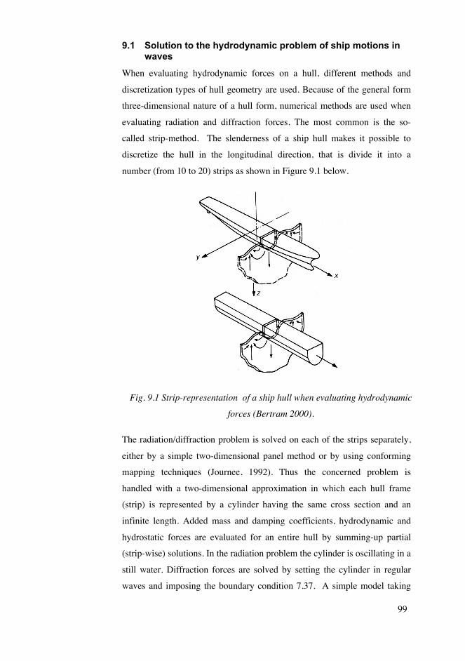
99
9.1 Solution to the hydrodynamic problem of ship motions in waves
When evaluating hydrodynamic forces on a hull, different methods and
discretization types of hull geometry are used. Because of the general form
three-dimensional nature of a hull form, numerical methods are used when
evaluating radiation and diffraction forces. The most common is the so-
called strip-method. The slenderness of a ship hull makes it possible to
discretize the hull in the longitudinal direction, that is divide it into a
number (from 10 to 20) strips as shown in Figure 9.1 below.
Fig. 9.1 Strip-representation of a ship hull when evaluating hydrodynamic
forces (Bertram 2000).
The radiation/diffraction problem is solved on each of the strips separately,
either by a simple two-dimensional panel method or by using conforming
mapping techniques (Journee, 1992). Thus the concerned problem is
handled with a two-dimensional approximation in which each hull frame
(strip) is represented by a cylinder having the same cross section and an
infinite length. Added mass and damping coefficients, hydrodynamic and
hydrostatic forces are evaluated for an entire hull by summing-up partial
(strip-wise) solutions. In the radiation problem the cylinder is oscillating in a
still water. Diffraction forces are solved by setting the cylinder in regular
waves and imposing the boundary condition 7.37. A simple model taking

100
into account the forward speed of the vessel is usually utilized. The methods
based on this approach are called strip methods. Details of the algorithms
will be not given in this textbook. The reader interested in them should refer
to the books and publications of Makoto Ohkusu, Johan Journee and
A.R.J.M. Lloyd.
There are also the 3-dimensional methods capable of solving the radiation
and diffraction problem without making the assumption of two-dimensional
flow nature. These potential flow theory based, so-called panel or boundary
element, methods can be divided into two classes in two different ways.
First, they can be divided according to computational domain. The solution
can be sought in the frequency domain or in the time domain. The frequency
domain means that a harmonic mono-chromatic small amplitude motion
(radiation problem) or wave of small amplitude (for in diffraction problem)
is considered at a time, and a solution is sought in in form of pressures in the
discrete points representing the hull up to the still water level. The process is
repeated for a number of frequencies covering the frequency range relevant
for ship motions or for the investigated wave-lengths. The problem is
linearized, which means that the wetted surface of a hull does not change
and extends to the still-water level. The pressures are summed up (Eq. 7.27)
and as a result of computations radiation forces for a unit ship motion added
masses and damping coefficients are obtained. Same is done for a wave of
unit amplitude and as a result diffraction forces are obtained.
Computation in the time domain makes it possible in principle to take
different nonlinearities into account; that is, pressures are evaluated for an
instantly wetted portion of the hull surface. In other words, in the latter case
pressures may be computed taking into account ship motions and wave
profile along the hull.
Another division of the methods is according to the type of Green function
used when evaluating the flow. In the so-called Green Function Method
(GFM), the flow domain is limited to the flat free surface level. Hull
discretization may be either extend to the still water level or take into
account variations in the wetted surface. A special, complicated form Green

101
function is used. This function automatically fulfils the boundary conditions
at the free surface.
In the Rankine Singularity Method (RSM), the Green function is of a very
simple form G=1/r, so the complicated, slowly converging oscillatory form
of the function does not have to be used. The drawback of RSM is the fact
that both ship hull surface and still water surface have to be discretized by
panels in this case. A comprehensive review of the methods briefly
described above is given for instance by Bertram (2000).
9.2 Outline of the solution of the linear ship motion in waves problem
The solution of equations 9.1 is usually sought in the frequency domain.
Thanks to the system’s linearity, the response to the regular that is
monochromatic, linear waves occurs at the frequency of encounter ωe which
is related to the wave frequency according to the equation 6.24. The
responses can be expressed in the non-dimensional form as
x(t)
A=x0
Acos ωet +γ x( ), y(t)
A=y0
Acos ωet +γ y( ),
z(t)
A=z0
Acos ωet +γ z( ),φ(t)
kA=φ0
kAcos ωet +γφ( ),
θ(t)
kA=θ0
kAcos ωet +γθ( ), ψ(t)
kA=ψ0
kAcos ωet +γψ( ).
(9.2)
Note that angular responses are made non-dimensional by dividing them by
wave steepness kA. Equations 9.1 suggest that the determination of
responses 9.2 is a straightforward task. However, it is not that easy and not
unified because of the complexity and due to different approaches used to
solve radiation and diffraction forces. It is customary to use the strip theory
approach described in Section 9.1. That is the hydrodynamic forces are
evaluated using a two-dimensional model for a finite number (10 to 20) of
ship hull sections. These forces are summed up in the total forces acting on
ship hull to be used in equations 9.1.

102
9.3 Transfer function of ship motion, response spectra
An example of the transfer functions of a modern passenger vessel is shown
in Figure 9.2.
Fig. 9.2 Transfer function of motions in waves of a RoPax vessel;
Fn=0.224.
For the sake of clarity, only RAOs of motion components are shown. It is
worth noting that transfer functions depend upon the ship’s speed and
heading. Normally, roll is the only motion component that exhibits resonant
behaviour. Sway, heave and pitch motion components are low for wave
lengths well below a ship’s length, and as expected, they are close to wave
amplitude or steepness for the long waves. There is no clear resonant
behaviour associated with them.
0.0
0.1
0.2
0.3
0.4
0.5
0 0.5 1 1.5 2 2.5 3 3.5 4
/L
x/A
90 deg 180 deg
0.00
0.50
1.00
1.50
0 0.5 1 1.5 2 2.5 3 3.5 4
y/A
l/L90 deg
0.0
0.2
0.4
0.6
0.8
1.0
1.2
0 0.5 1 1.5 2 2.5 3 3.5 4
/L
z/A
90 deg 180 deg
0.0
0.5
1.0
1.5
2.0
2.5
3.0
0 0.5 1 1.5 2 2.5 3 3.5 4
/L
/(kA
)
90 deg 180 deg
0
0.2
0.4
0.6
0.8
1
1.2
0 0.5 1 1.5 2 2.5 3 3.5 4
/L
/(kA
)
90 deg 180 deg
0
0.02
0.04
0.06
0.08
0.1
0 0.5 1 1.5 2 2.5 3 3.5 4
/L
/(kA
90 deg 180 deg

103
The linear ship dynamics model does not predict non-symmetric ship
motions in the symmetrically acting waves. For this reason, for the head and
the following waves, RAOs of roll, sway and yaw are zero.
Transfer functions of a ship, such as these presented in Figure 9.2, can be
obtained using some of the linear approximation based strip theories or
experimentally by conducting model tests in regular waves.
One of the benefits of using the linear wave and ship dynamics models is the
possibility of evaluating, in a straightforward manner, spectra of ship
motions in irregular waves given by spectrum S(ω). This is done by the
following operation
Sr (ωe ) = H(ωe )2S(ωe ) = RAO2S(ωe ), (9.3)
where Sr is the power spectral density of the response in question and H(ωe)
is the transfer function comprising RAO and phase information. Operation
9.3 is presented in Figure 9.3 below.
Fig. 9.3 Calculation of heave motion in irregular waves.
It should be noted that the frequency of encounter is used as an argument
when evaluating response spectra. Sometimes another definition of RAO is
used. In this definition, by RAO, the absolute value of transfer function
squared is meant, that is RAO=|H(ω)|2. The spectrum of the encountered

104
waves can be derived assuming that the wave spectrum S(ω) is given and
using the relation 6.24. The differential equation
dω e
dω= 1−
2Vωgcosμ
(9.4)
is obtained by differentiating equation 6.24. The wave energy contained
within the frequency bandwidths dω and dωe is not affected by ship motion.
This means that the following holds
S ωe( )dωe = S ω( )dω (9.5)
and as a result the wave spectrum in terms of the encounter frequency is
given by
S ωe( ) = S ω( ) dωdωe
= S ω( ) g
g− 2Vω cosμ . (9.6)
Transformation 9.6 yields an increase in frequency and thus is visible as a
shift of power density towards higher frequencies for head and bow waves
(see Fig. 9.4).
Fig. 9.4 Wave power spectrum of the Jonswap type (Hs=4.7 m, T1=7.5 s) as
measured by a stationary buoy (left figure) and felt by a ship proceeding at a
speed of 14 knots and heading angle of 135 [degrees] (right figure).
Having the power spectral density of the response in question evaluated with
the aid of Equation 9.3, it is easy to derive the root-mean-square (rms) value
from

105
σ 0 = m0 , (9.7)
where m0 is zero-th spectral moment defined by Equation 6.40. The rms
values of the time derivatives of the response in question are given by
σ 2 = m2 (9.8)
for the velocity and
σ 4 = m4 (9.9)
for the acceleration.
When evaluating the angular responses of a ship in irregular waves, it is
feasible to use the spectrum of wave slopes instead of the spectrum of
amplitudes. Knowing that for a deep water condition the slope of each wave
component is kA=Aω2/g, the spectrum Sα(ω) of wave slopes is
Sα ω( ) = ω4
g2S ω( ).
(9.10)
Another way of evaluating the responses in irregular waves is based on
using the wave frequency rather than applying the frequency of encounter.
In this approach the response spectra are obtained by the operation
Sr (ω) = H(ω) 2S(ω) (9.11)
for the linear responses, and by
Sr (ω)= H (ω)2Sα (ω)
(9.12)
in case of angular responses. These spectral densities do not have much
physical meaning but they can be transferred to the meaningful frequency of
encounter equation 9.6. Using the wave frequencies ω when evaluating the
responses in irregular waves is particularly useful for the following and
106
quartering waves, as it avoids the complexities of multi-valued spectral
ordinates at the same encounter frequency (Lloyd, 1989).

107
10. Nonlinear model of ship motion in waves
If non-linear terms of the equations of motion (equations 4.4 and 4.7 and
non-linear hydrodynamic terms discussed in Chapters 5 to 7) are to be
included in the ship motion simulation than solution can not be sought in a
frequency domain. Neither a powerfull and very usefull concept of transfer
function can be used. Nonlinear mathematical model has to be solved in a
time-domain instead. Ship motions in waves can be solved by integrating
numerically the general non-linear equations of motions presented in
Chapter 4 with the appropriate model of hydrodynamic reaction and
excitation forces. When integrated, these equations yield velocitities
U=ui+vj+wk and ΩΩ=pi+qj+rk in terms of their components expressed in the
body-fixed, that is moving, co-ordinate system. In order to obtain the
information on ship position in respect to the inertial Earth-fixed frame,
these velocity components are projected on the Earth-fixed co-ordinate
system and integrated into the position vector and Euler angles.
Ship resistance in still water, thrust of propeller(s), rudder forces and wind
forces are evaluated as discussed in sub-chapters 5.6, 5.7 or 5.8 and 5.10.
Hydrodynamic reaction forces due to the manoeuvring and excitation due to
waves have to be taken into account when applying the models of Section
5.6 and Chapter 7. If manoeuvring in waves is of concern, there is the
problem of different time scales and different hydrodynamic reaction forces
associated with them. The so-called slow motion hydrodynamic derivatives
of Section 5.6 were evaluated for the still water condition. Thus their
application for the ship operating in waves may be questioned. A good
compromise is to preserve only the terms related to velocities such as

108
Yv,Yr,Nv and Nr . The argument is that these terms include the effects that
are related to slow motion, and they are mainly governed by the non-
potential flow effects. The terms related to the accelerations are taken as
added masses being related to the radiation forces (Sub-Section 7.6), with
the flow memory effect being included.
10.1 Direct evaluation of ship responses in time domain used in the program LaiDyn
The equations of motion solved in time domain and resulting in a simulation
of ship motions in waves are given below.
m+a11( )u+a15q = −mgsinθ + Xresistance + Xprop + Xrudder + Xwave + Xman
−k15 + m+a22( ) rv−qw( )m+a22( )v+a24 p+a26r =mgcosθ sinφ + m+a11( ) pw− ru( )+Yman
+Yrudder +Ywave − k22 − k24 − k26m+a33( )w+a35q = mgcosθ cosφ +m uq− vp( )+ Zwave − k33 − k35
a42v+ Ix+a44( ) p+a46r = Iy − Iz( )qr −Yrudderzrudder +Kman +Kwave − k44
−k42 − k46 +2ζ pωφ
a15u+a53w+ Iy+a55( )q = Iy − Ix( ) pr+ Xrudderxrudder +Mwave − k55 − k53 − k15
a62v+a64 p+ Iz+a66( )r = Ix − Iy( ) pq+Yrudderxrudder +Nman +Nwave
−k66 − k62 − k64 (10.1)
In principle, the above equations are the same as the ones discussed in
Chapter 4 (equations 4.4 and 4.7). The difference is in an explicit inclusion
of the hydrodynamic terms, which are discussed below.
Discussion of the terms included in the above equations of motion.
Radiation terms
The terms aij and kij are the added mass coefficients corresponding to the
infinite frequency and elements of the memory function respectively, as
described in Section 7.6.
Manoeuvring terms
The terms depicted by subscript ‘man’ are the manoeuvring forces and
moments represented by hull forces related to yaw and sway velocities.
When evaluating them one of the models used in a manoeuvring simulation

109
(such as the one given by expressions 5.31) is used. In other words, the
effect of ship motions in waves is disregarded when evaluating the slower
wave-induced motion of a ship. It is worth noting that the terms related to
yaw and sway accelerations are included in the radiation model.
Resistance and thrust
Still water resistance for a vessel on a straight course with no drift is
represented by the term Xresistance. Thrust generated by a propeller is depicted
by Xprop. They are evaluated as described in Section 5.7.
Rudder
The subscript ‘rudder’ refers to rudder forces and to the location of the
rudder in the body-fixed co-ordinate system. The forces are evaluated as
presented in the Section 5.8.
Restoring forces and wave loads
Forces and moments depicted with subscript ‘wave’ are the ones
incorporating the restoring forces and moments as well as the wave loads.
For the irregular waves nonlinear hydrostatic and Froude-Krylov pressures
are evaluated as described in Section 7.5, but summing up the contributions
of several wave components. That is, wave elevation above the control point
C is given by
ζ t( ) =i=1
N
∑ Ai cos k i Xc cosμ −Yc sinμ( )−ωit +δi⎡⎣ ⎤⎦, (10.2)
where Xc and Yc are the control points of the hull surface given in the Earth-
fixed co-ordinate system XYZ given by the transformation 7.23. The co-
ordinates Xc and Yc take into account the ship’s position in waves. ki=ωi/g is
the wave number corresponding to the i-th wave component. For the
immersed panel, that is, for Zc+ζ(t)>0, pressure is evaluated from the
expression
110
pc t( ) = ρg Zc +i=1
N
∑ Ai exp −ki[Zc +ζ (t)]{ }⎧⎨⎩
icos k i Xc cosμ −Yc sinμ( )−ωit +δi⎡⎣ ⎤⎦}.
(10.3)
The argument of the exponent function in (10.3) satisfies the dynamic
boundary condition at the actual water surface. The pressure profile thus
obtained is sometimes called as the stretched one. This approach is a kind of
extension of the linear wave theory to incorporate nonlinear effects
associated with the variation of a ship’s wetted surface. Refer to figures 7.2
and 7.3 for the quantities used in evaluating hydrostatic and Froude-Krylov
pressures. The position of the control point C in the inertial co-ordinate
system XYZ is obtained from the transformation given by equation 7.23.
Diffraction part of the wave load is taken from the linear seakeeping theory.
Additional damping of roll
An allowance for a viscous damping of roll is incorporated in the fourth
equation. In the second line of this equation, ζ stands for the critical
damping ratio and ωφ stands for the natural roll angular frequency.
The solution of nonlinear differential equations of motion 10.1 in the time-
domain can be obtained by integrating them using an appropriate numerical
procedure and applying a sufficiently small time step.
On the left-hand side of equations 10.1, several terms related to motion
accelerations occur in each of the equations. This means that equations are
coupled and cannot be solved as such. Before solving, equations 10.1 have
to be de-coupled. This is done numerically at each time step as follows. The
equations 10.1 can be expressed in the matrix form as
A i x = B , (10.4)
where matrix

111
A =
m+a11 0 0 0 a15 0
0 m+a22 0 a24 0 a260 0 m+a33 0 a35 0
0 a42 0 Ix+a44 0 a46a15 0 a53 0 Iy+a55 0
0 a62 0 a64 0 Iz+a66
⎡
⎣
⎢⎢⎢⎢⎢⎢⎢⎢
⎤
⎦
⎥⎥⎥⎥⎥⎥⎥⎥
,
vector comprising accelerations is given by:
x =
uvwp
q
r
⎧
⎨
⎪⎪⎪
⎩
⎪⎪⎪
⎫
⎬
⎪⎪⎪
⎭
⎪⎪⎪
= u,v,w, p,q, r{ }T
and vector B is built-up by the right-hand sides of equations 10.1 as follows:
B =
−mgsinθ + Xresistance + Xprop + Xrudder + Xwave + Xman − k15 + m+a22( ) rv−qw( )mgcosθ sinφ + m+a11( ) pw− ru( )+Yman +Yrudder +Ywave − k22 − k24 − k26
mgcosθ cosφ +m uq− vp( )+ Zwave − k33 − k35
Iy − Iz( )qr −Yrudderzrudder +Kman +Kwave − k44 − k42 − k46 +2ζ pωφ
Iy − Ix( ) pr+ Xrudderxrudder +Mwave − k55 − k53 − k15
Ix − Iy( ) pq+Yrudderxrudder +Nman +Nwave − k66 − k62 − k64
⎧
⎨
⎪⎪⎪⎪⎪
⎩
⎪⎪⎪⎪⎪
⎫
⎬
⎪⎪⎪⎪⎪
⎭
⎪⎪⎪⎪⎪
Equation 10.4 can be written as
A−1 iA i x = x = A−1 iB . (10.5)
As a result we have obtained a set of six nonlinear normal second order
differential equations with acceleration terms (vector x ) on the left-hand –
side of the matrix equation 10.5. This set of equations 10.5 is integrated
numerically using the Runge-Kutta fourth-order scheme yielding velocity
vector x = u,v,w, p,q, r{ }T
.
Next, at the same time step, the transformation given by expression 3.7 is
used to project the velocities on the axes of Earth-fixed co-ordinate system.
The projected velocities are integrated numerically using also the same

112
Runge-Kutta routine. The position of the ship, given by the vector
X = XG ,YG ,ZG ,φ,θ ,ψ{ }T
at each time step is obtained as a result.
10.2 Linear approximation to ship motions in irregular long-crested waves
Linear approximation to the global responses of a ship in irregular waves is
evaluated in order to judge the effects of nonlinearity on the derived
responses. Normally, in the linear seakeeping theory, a constant forward
speed is assumed. In the Laidyn method, surge motion of a ship is evaluated
in the time domain taking into account, amongst the others, propeller action
and variations of the wetted surface. Thus in-plane motion of a ship is
simulated in a time domain along with the other motion components. This
results in ship position XG,YG in the Earth-fixed co-ordinate system. This, in
addition to the knowledge of transfer functions of the corresponding
responses, makes it possible to evaluate the linear approximation of the
responses using the expressions
xL t( ) =i=1
N
∑ AixL0 (ω i,μ)cos k i XG cosμ −YG sinμ( )−ω it +δ i −γ x,i⎡⎣ ⎤⎦
yL t( ) =i=1
N
∑ AiyL0 (ω i,μ)cos k i XG cosμ −YG sinμ( )−ω it +δ i −γ y,i⎡⎣ ⎤⎦
zL t( ) =i=1
N
∑ AizL0 (ω i,μ)cos k i XG cosμ −YG sinμ( )−ω it +δ i −γ z,i⎡⎣ ⎤⎦
φL t( ) = k ii=1
N
∑ AiφL0 (ω i,μ)cos k i XG cosμ −YG sinμ( )−ω it +δ i −γ φ,i⎡⎣ ⎤⎦
θL t( ) = k ii=1
N
∑ AiθL0 (ω i,μ)cos k i XG cosμ −YG sinμ( )−ω it +δ i −γ θ ,i⎡⎣ ⎤⎦
ψ L t( ) = k ii=1
N
∑ Aiψ L0 (ω i,μ)cos k i XG cosμ −YG sinμ( )−ω it +δ i −γ ψ ,i⎡⎣ ⎤⎦,
(10.6)
where terms with subscripts L0 depict gain factors of the transfer functions
and γ the corresponding phase angles.
10.3 More on the numerical solution
The solution to the problem starts with the linear approximation 9.1 yielding
the transfer functions 9.2. Added masses and damping coefficients and their

113
dependence upon the frequency are also evaluated by the linear strip theory
based seakeeping method (Journee, 1992). These coefficients are
transformed to the co-ordinate system having an origin in the ship’s centre
of gravity G as described in Appendix B. After that, the convolution
integrals are evaluated with the aid of the Fast-Fourier-Transform algorithm
yielding the retardation functions 7.34. The details are given in Appendix C
There are two options in the Laidyn method. In the first version, the
responses are solved by a direct integration of the equations as discussed in
the preceeding paragraph. An interesting option to the solution is the so-
called Two-stage approach described in the following paragraph.
In both solution strategies, the zero initial conditions are used for all
equations with the exception of surge velocity, which is set initially to a
prescribed ship velocity in calm water. In order to damp spurious transients,
the wave amplitude is gradually increased from zero to the prescribed final
value Afinal using the expression
A(t) = Afinal 1− cosπt
2Tf
⎛
⎝ ⎜ ⎜
⎞
⎠ ⎟ ⎟
2⎡
⎣ ⎢ ⎢
⎤
⎦ ⎥ ⎥ for t < Tf
A(t) = Afinal for t ≥ Tf ,
(10.7)
with Tf= 50 seconds in full scale being used.
10.4 Two-stage approach
Instead of solving the nonlinear equations of motions directly, it is possible
to apply the so-called two-stage approach to the non-linear set of equations
of motion.
Illustration of the two-stage approach using a single-
degree-of-freedom nonlinear system
For the sake of simplicity the two-stage approach is explained in this section
using a single-degree-of-freedom model. Let us consider a single-degree-of-
freedom system given by a nonlinear equation

114
mX + g(X)+h(X)= F(X;t), (10.8)
where m is the system mass and t is the time. The functions g and h are in
general nonlinear functions of response velocity ˙ X and displacement X,
respectively. Function F is also a nonlinear function of X describing the
external excitation of the system. The linear version of the equation (10.8) is
given by
mxL + cxL + kxL = FL (t), (10.9)
where FL is a linear, independent of the response forcing function. The total
response is decomposed into a linear part xL and a nonlinear portion x as
X = xL + x. (10.10)
Subtracting linear approximation (10.9) from the general equation (10.8)
yields an equation for the non-linear part x of the response
mx+ g(xL + x)− cxL[ ]+ h(xL + x)− kxL[ ] = f , (10.11)
where f = F(X;t) – FL(t) is the nonlinear part of the forcing function.
In the two-stage approach, nonlinear differential equation (10.8) is solved by
solving first the linear version (10.9) of it. Next, the nonlinear part x of the
response is derived by solving numerically (10.11) with a known linear
solution xL. The total solution is evaluated using a sum (10.10).

115
11. Some applications of the theory
11.1 Capsizing of a ship in steep regular waves
Two ship cases were used in the benchmark study initiated by the
International Towing Tank Conference and presented in the 23rd ITTC
(2002). The first vessel, ship A1, is a containership with a waterline length
of LPP = 150 m and a low metacentric height (GM0 = 0.15 m). This low GM0
value means that the static stability of the ship is poor. The second vessel
ship A, is a model of a fishing vessel with the length LPP = 35.68 [m]. Both
models were run in regular waves, different headings and Froude numbers (
Fn = VSgLPP
). The summary of the model test results and simulation results
are given in two Tables 11.1 and 11.2. Wavelength is denoted by λ and aW is
the wave amplitude.
Table 11.1 Summary of the results for the containership (Ship A1).
Case λ/Lpp 2AW/ λ Fn
Heading μ
[deg] Experiment Computed
1 1.5 1/25 0.2 0
Parametric roll
resonance, capsize
Parametric roll
resonance, no
capsizing
2 1.5 1/25 0.2 45 No capsizing No capsizing
3 1.5 1/25 0.3 30 No capsizing No capsizing
4 1.5 1/25 0.4 30 Capsize Capsize
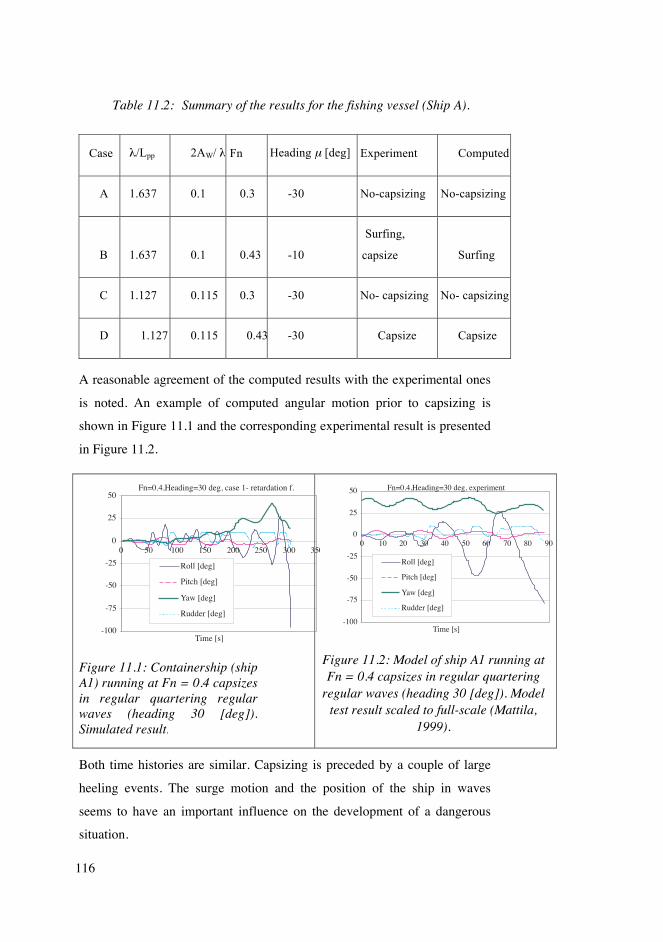
116
Table 11.2: Summary of the results for the fishing vessel (Ship A).
Case λ/Lpp 2AW/ λ Fn Heading μ [deg] Experiment Computed
A 1.637 0.1 0.3 -30 No-capsizing No-capsizing
B 1.637 0.1 0.43 -10
Surfing,
capsize Surfing
C 1.127 0.115 0.3 -30 No- capsizing No- capsizing
D 1.127 0.115 0.43 -30 Capsize Capsize
A reasonable agreement of the computed results with the experimental ones
is noted. An example of computed angular motion prior to capsizing is
shown in Figure 11.1 and the corresponding experimental result is presented
in Figure 11.2.
Figure 11.1: Containership (ship A1) running at Fn = 0.4 capsizes in regular quartering regular waves (heading 30 [deg]). Simulated result.
Figure 11.2: Model of ship A1 running at Fn = 0.4 capsizes in regular quartering
regular waves (heading 30 [deg]). Model test result scaled to full-scale (Mattila,
1999).
Both time histories are similar. Capsizing is preceded by a couple of large
heeling events. The surge motion and the position of the ship in waves
seems to have an important influence on the development of a dangerous
situation.
Fn=0.4,Heading=30 deg, case 1- retardation f.
-100
-75
-50
-25
0
25
50
0 50 100 150 200 250 300 350
Time [s]
Roll [deg]
Pitch [deg]
Yaw [deg]
Rudder [deg]
Fn=0.4,Heading=30 deg, experiment
-100
-75
-50
-25
0
25
50
0 10 20 30 40 50 60 70 80 90
Time [s]
Roll [deg]
Pitch [deg]
Yaw [deg]
Rudder [deg]

117
11.2 Parametric rolling in regular waves
Parametric roll resonance is an unexpected ship roll motion in head or
following seas. The phenomenon is known to shipmasters. Linear
seakeeping theory is not capable of predicting this roll motion; and for this
reason, we can call it an unexpected response. The phenomenon is generally
attributed to the parametric variation of the restoring moment of heel caused
by a large variation in the water-plane area in waves. Thus, qualitatively, the
phenomenon is often described by a single equation of the Mathieu type.
An extensive model test series of a modern, fast twin-screw Ro-Pax vessel
was conducted at the Ship Laboratory of the Helsinki University of
Technology. Tests were primarily concerned with the dynamic stability. In
particular, a loss of stability on a crest of a following wave and parametric
roll resonance were investigated both in regular and irregular waves for
three KG values with a ship model without and with two different height
bilge keels (450 mm and 900 mm in the full scale). Tests were run with the
self-propelled model steered manually (Mattila, 1999). The main particulars
of the vessel are given in Table 11.3.
The stability lever curve of the vessel is shown in Fig. 11.3
Fig. 11.3 Static stability lever curve of the investigated vessel for the height of
the centre of gravity KG = 12 [m].
In the following figures 11.4 and 11.5, example time histories of motions
corresponding to only a single test case are presented.
0
0.2
0.4
0.6
0.8
1
0 10 20 30 40 50
GZ
[m]
Heel [deg]

118
Table 11.3 Main particulars of the vessel Seatech-D
Full scale Model Scale
1 39.024
Lwl [m] 158.6 4.064
Lpp [m] 158 4.049
Dp [m] 4.8 0.123
B [m] 25 0.641
Bwl [m] 25 0.641
Ta [m] 6.1 0.156
Tφ [m] 6.1 0.156
D [m] 15 0.384
∇ [m3] 13766 0.232
Mm [kg] 231.40
S [m2] 4356 2.860
CB 0.571 0.571
Lwl/Bwl 6.344 6.344
Bwl/Twl 4.098 4.098
Lwl/∇(1/3) 6.618 6.618
KG [m] 11, 11.5, 12 0.282, 0.295, 0.307

119
Fig. 11.4 Simulated angular motions for a ship with low bilge keels and KG =
12 m. Wave amplitude A=1.7 [m]. Tφ = 20 [s], ξ = 0.046. Ultimate roll
amplitude is 16 [deg].
Fig. 11.5 Measured roll for a ship equipped with low bilge keels and KG = 12
m. Wave amplitude A=1.7 [m]. Tφ = 20 [s], ξ = 0.046.
Both the simulations and the model test experiments gave similar
conclusion. In this case of a pure parametric resonance, where the ratio of an
encounter period to roll natural period is 0.5, roll amplitude seems to be
related to wave amplitude squared. Moreover, an increase of the wave
amplitude results in a lower number of encounter periods required for a roll
motion to start. Simulations indicated that there is a certain threshold value
of wave amplitude below which parametric roll resonance does not develop.
Fn=0.13, =244 m, Aw=1.7 m
-15
-10
-5
0
5
10
15
360 420 480 540 600 660
time [s]
Roll Pitch Yaw
Measured roll, Fn=0.13, =244m,Aw=1.7m
-25
-20
-15
-10
-5
0
5
10
15
20
25
60 120 180 240 300 360
Time [s]

120
Both the simulations and the tests indicated that an increase in damping,
achieved by bilge keels, results in a somewhat lower roll amplitude.
Damping also delays and slows the development of the parametric roll
resonance (Matusiak, 2003).
11.3 Time-domain simulation of the weather criterion
In order to ensure the safety of a vessel in a ‘dead ship condition’, the so-
called weather criterion was made mandatory for ships in 2005. The
criterion takes into account resonant beam waves and gusty wind (IMO). As
the origin of the criterion is quite old and there are a number of strong
assumptions involved, its application to a modern large size passenger
vessel can be questioned. In order to make it better-suited for modern ships,
an allowance for the alternative assessment using model tests was made.
Tests are believed to yield more realistic values of wind loading and better
estimates of roll amplitude at the resonance. The first attempts to utilize
model tests in validating fulfilment of the weather criterion were presented
in Yon (2006) and Ishida (2006).
The LAIDYN method was used to evaluate the fulfilment of the weather
criterion by an example passenger ship design (Matusiak&Hamberg, 2006).
The original idea was to substitute the model tests of the alternative
assessment with the appropriate numerical simulations. The interesting
findings of this study were:
The so-called “effective” roll-back angle obtained by simulating a ship’s
behaviour in beam seas was very close to the one given by the rule (-5 [deg]
in the considered case).
Weather criterion considers the resonant beam seas as a critical situation
yielding an initial heel at which wind gust impacts the vessel. Wave action
as such is disregarded when considering the transient response of the ship
caused by heeling moment due gusty wind loading. Thus the fulfilment of
the weather criterion can be simulated (numerically or with the aid of model
tests) by investigating ship’s transient heel response in still water with an

121
initial value set by a roll-back angle and step-wise heeling moment
simulating gusty wind. The simulated result of this kind of response is
shown in Figure 11.6 with ship heeling by 27 [deg]. The corresponding
situation, as evaluated traditionally with the aid of the dynamic lever
concept, is shown in Figure 11.7 and yields maximum heeling of 30 [deg].
Fig. 11.6 Ship transient rolling caused by the gusty wind and initial heel. Gust
loading is taken according to the weather criterion.
Fig. 11.7. Ship dynamic heeling according to the weather criterion. lw is
dynamic lever of gusty wind loading and e is dynamic lever of the restoring
moment (integral over the GZ curve).
Transient roll motion due to a gusty wind
and initial heel
-10
-5
0
5
10
15
20
25
30
0 30 60 90 120 150 180
time [s]
0
0.05
0.1
0.15
0.2
0.25
-5 0 5 10 15 20 25 30
Heel [deg]
e [m•rad] lw
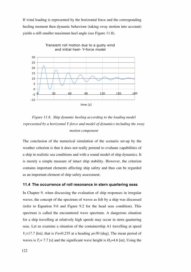
122
If wind loading is represented by the horizontal force and the corresponding
heeling moment then dynamic behaviour (taking sway motion into account)
yields a still smaller maximum heel angle (see Figure 11.8).
Figure 11.8. Ship dynamic heeling according to the loading model
represented by a horizontal Y-force and model of dynamics including the sway
motion component
The conclusion of the numerical simulation of the scenario set-up by the
weather criterion is that it does not really pretend to evaluate capabilities of
a ship in realistic sea conditions and with a sound model of ship dynamics. It
is merely a simple measure of intact ship stability. However, the criterion
contains important elements affecting ship safety and thus can be regarded
as an important element of ship safety assessment.
11.4 The occurrence of roll resonance in stern quartering seas
In Chapter 9, when discussing the evaluation of ship responses in irregular
waves, the concept of the spectrum of waves as felt by a ship was discussed
(refer to Equation 9.6 and Figure 9.2 for the head seas condition). This
spectrum is called the encountered wave spectrum. A dangerous situation
for a ship travelling at relatively high speeds may occur in stern quartering
seas. Let us examine a situation of the containership A1 travelling at speed
Vs=17.7 [kn], that is Fn=0.235 at a heading μ=30 [deg]. The mean period of
waves is T1= 7.7 [s] and the significant wave height is HS=4.6 [m]. Using the
Transient roll motion due to a gusty wind
and initial heel- Y-force model
-10
-5
0
5
10
15
20
25
30
0 30 60 90 120 150 180
time [s]
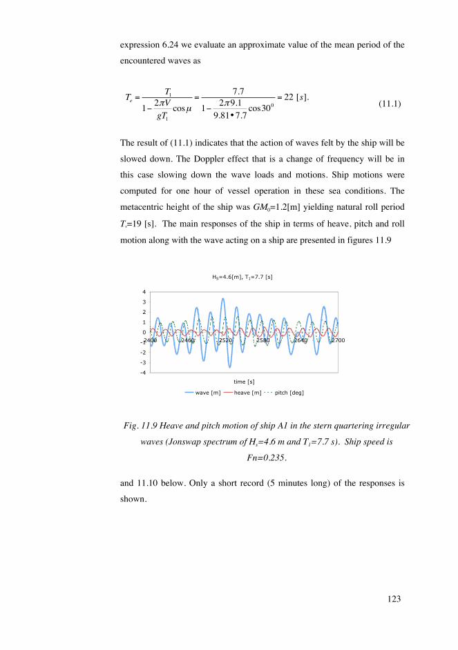
123
expression 6.24 we evaluate an approximate value of the mean period of the
encountered waves as
Te = T1
1−2πVgT1
cosμ=
7.7
1−2π9.1
9.81•7.7cos300
= 22 [s].
(11.1)
The result of (11.1) indicates that the action of waves felt by the ship will be
slowed down. The Doppler effect that is a change of frequency will be in
this case slowing down the wave loads and motions. Ship motions were
computed for one hour of vessel operation in these sea conditions. The
metacentric height of the ship was GM0=1.2[m] yielding natural roll period
Tφ=19 [s]. The main responses of the ship in terms of heave, pitch and roll
motion along with the wave acting on a ship are presented in figures 11.9
Fig. 11.9 Heave and pitch motion of ship A1 in the stern quartering irregular
waves (Jonswap spectrum of Hs=4.6 m and T1=7.7 s). Ship speed is
Fn=0.235.
and 11.10 below. Only a short record (5 minutes long) of the responses is
shown.
HS=4.6[m], T1=7.7 [s]
-4
-3
-2
-1
0
1
2
3
4
2400 2460 2520 2580 2640 2700
time [s]
wave [m] heave [m] pitch [deg]

124
Figure 11.10 Ship A1 rolls in the stern quartering irregular waves (Jonswap
spectrum of Hs=4.6 m and T1=7.7 s). Ship speed is Fn=0.235 and
metacentric height GM0=1.2 m.
An interesting feature of the encountered waves is noted. Although the
amplitude of the waves changes, the period of the wave train seems to be
nearly constant, at least for the selected record. The mean value of the
encounter period is 20 [s], which is close both to the estimate given by
formula 11.1 and to the natural roll period of ship. Fourier analysis of the
encountered waves was conducted and the results of it are presented in
Figure 11.11 below.
Figure 11.11 The effect of ship speed (Fn=0.235) and course in respect to
wave propagation direction (μ=300) on the waves encountered by a ship.
HS=4.6[m], T1=7.7 [s]
-10
-5
0
5
10
15
2400 2460 2520 2580 2640 2700
time [s]
Rol
l [de
g]
wave [m] roll [deg]
HS=4.6 [m]
0
5
10
15
20
25
0 0.2 0.4 0.6 0.8 1 1.2 1.4
ω [rad/s]
S(w
ave)
S (encountered) S (stationary)
T1=19.7 [s]
T1=7.7 [s]

125
Apart form a shift in frequency content towards lower values, a sharpening
of the spectrum of the encountered waves is noted. This means that in this
condition, waves of different lengths act on the ship with nearly the same
frequency. As this frequency (encounter frequency) is close to the natural
frequency of roll, a resonance of roll motion occurs.
Next we check what will be the effect of decreasing ship speed to 12 knots.
The spectra of encountered and stationary waves are shown in Figure 11.12
below.
Lowering the ship speed to 12 knots decreases the mean value of the
encounter period to T1=13 [s]. This is sufficiently away from the natural roll
period. As a result ship roll motion decreases radically.
Figure 11.12 The effect of ship speed (Fn=0.16) and course with respect to
wave propagation direction (μ=300) on the waves encountered by a ship.
In Figure 11.13 shows a record 5 minutes in length comprising the
maximum roll motion experienced by the ship within an hour of operation.
HS=4.6 [m]
0
5
10
15
20
25
30
35
0 0.2 0.4 0.6 0.8 1 1.2 1.4
ω [rad/s]
S(w
ave)
S (encountered) S (stationary)
T1=13 [s]
T1=7.7 [s]

126
Figure 11.13 Ship A1 rolls modestly in the stern quartering irregular waves
(Jonswap spectrum of Hs=4.6 m and T1=7.7 s). Ship speed is Fn=0.16 and
metacentric height GM0=1.2 m.
It is clear that in the considered sea condition and ship’s heading, the high
speed of the vessel, may lead to a dangerous situation. The danger of
running a ship at high speed in stern quartering seas is recognized by IMO,
which has Revised Guidance to The Master For Avoiding Dangerous
Situations in Adverse Weather and Sea Conditions (2007).
Claus Stigler (2012) has investigated the same phenomenon using the
RoPax ship model (Seatech-D) presented in Chapter 11 and in Section 10.2.
A self-propelled model was radio-controlled in tests conducted in the
multifunctional model basin at Aalto University. The height of Centre-Of-
Gravity was adjusted so that the natural roll period in the model scale was 3
s, that is, it corresponded to the full-scale value Tφ=18.75 s. The turning
circle tests were run in the basin in irregular waves given by the significant
wave height HS=4.8 m and an average period T1=5.9 s. Speed of the model
was controlled manually by adjusting the revolutions of propellers. The
target value of it was VS=16.5 kn full-scale. This creates a dangerous
situation of roll resonance in stern quartering seas. A typical behaviour of a
model in the resonance condition is presented in Figure 11.14 below.
HS=4.6 [m], T1=7.7 [s]
-10
-5
0
5
10
15
2370 2430 2490 2550 2610 2670 2730
time [s]
Rol
l [de
g]
wave [m] roll [deg]
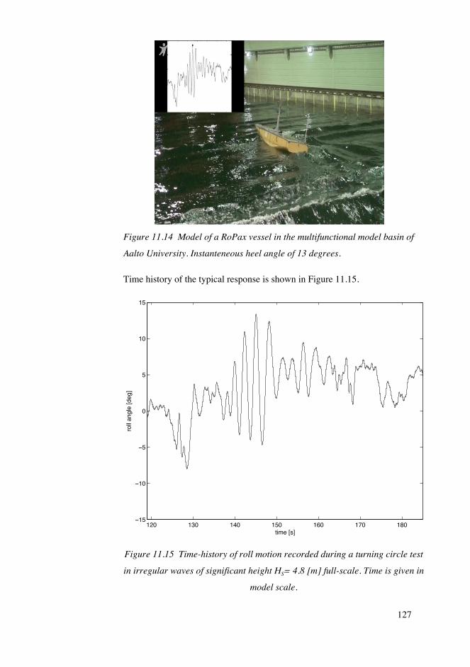
127
Figure 11.14 Model of a RoPax vessel in the multifunctional model basin of
Aalto University. Instanteneous heel angle of 13 degrees.
Time history of the typical response is shown in Figure 11.15.
Figure 11.15 Time-history of roll motion recorded during a turning circle test
in irregular waves of significant height HS= 4.8 [m] full-scale. Time is given in
model scale.

128
Simulated ship motion, corresponding to the conditions of the model test, is
presented in Figure 11.16 below.
Figure 11.16 Simulated turning circle test in irregular waves of a significant
wave height HS= 4.8 [m].
Despite different wave trains of irregular waves realizations, measured and
simulated roll motion are quite similar. The simulated maxima of roll
amplitude are close to the measured ones. A steady heel caused by a
centrifugal force effect is noted in both signals. As the simulated turning
circle is somewhat smaller, the steady heel for a simulated test is slightly
larger. Roll motion develops in stern quartering seas as an unfavourable
effect of a change in frequency of encounter. This is clearly seen in the time-
history of the simulated waves encountered by a ship. In critical conditions,
short and long waves act on a ship with a period close to the natural roll
period (Tφ=19 [s]). This is a primary reason for roll motion that may
endanger ship operation. It is worth noting that reducing the speed of a ship
or change in the heading suppresses the danger in this case.

129
12. Internal loads acting on a rigid hull girder
Apart from a ship's rigid body motion, it is important to know the internal
forces and moments that act on a hull of a ship operating in waves. These
forces are primarily composed of mass and hull/water interaction forces. In
still water, the mass force (or its distribution) is simply the distributed ship
weight. Hull/water interaction force, in this case, is the buoyancy or its
distribution in the form of hydrostatic pressure. In waves, mass forces get an
additional contributor associated with accelerations due to ship motions. As
a result, the inertia component is added to the weight. Moreover, hull/water
interaction gets more complicated. As described in Chapter 7, pressure
acting on a hull surface in waves comprises, apart from the hydrostatic part,
the radiation, Froude-Krylov and diffraction contributions.
The predictions of the wave-induced primary stresses are important in the
ultimate strength assessment of the hull girder. If the hull girder has
compression on deck, it is called a sagging condition. If there is
compression on the bottom, it is called a hogging condition. (See Figure
12.1.)

130
Figure 12.1 Hull sagging and hogging.
In waves, the sagging condition occurs if wave crests are at the bow and
stern and hogging occurs if a wave crest is at mid-ship. The sagging
increases if the ship has large bow flare and the ship motions are large with
respect to waves. The stern form of the ship can have the same effect if the
ship has a flat bottom stern close to the waterline. In the structural design of
ships, a common practice is to express the extreme design loads by means of
the sagging and hogging bending moments and shear forces. The sagging
and hogging bending moments and shear forces are hull girder loads. The
hull girder loads are internal forces and moments affecting a cross-section of
the ship hull. The accurate prediction of the extreme wave loads is important
in the ultimate strength assessment of the hull girder. For ships in a heavy
sea, the sagging loads are larger than the hogging loads. The linear theories
cannot predict the differences between sagging and hogging loads
(Kukkanen, 2012).
12.1 Linear approach
We start discussion of internal loads with a simple linear model, which is
normally a part of a linear strip-theory approach to a solution of ship

131
motions in waves (discussed in paragraph 9.1). We shall adopt the body-
fixed co-ordinate system, which is often called ‘the sea-keeping co-ordinate
system as presented in Figure 12.2 below.
Figure 12.2 Definition of the ship-fixed co-ordinate system and
the motion components used by Kukkanen (2012)
For the sake of simplicity, we shall limit the discussion to the global load in
terms of vertical shear force and the bending moment acting on a hull
regarded as a beam resting on a flexible foundation. First we consider a hull
in still water. At each station, denoted by a position x, we have the vertical
force per unit length given by a sum of weight and buoyancy at this section,
that is
q(x)= −m(x)g+ ρgA(x), (12.1)
where m(x) is mass of the hull per unit length and A(x) is the sectional frame
area. With ship heaving η3 and pitching η5 motion, we have to also take
inertia and hydrodynamic F(x) loads as well. As a result, the vertical force
per unit length of a hull gets the form

132
q(x) = −m(x)g + ρgA(x)−m(x) η3 − xη5( ) + F (x) (12.2)
Total vertical shear force and bending moment at section xp can be obtained
by integrating load 12.2 along the ship length from the stern up to the
section x’p as follows
Q(x 'p ) = q(x ')0
x 'p
∫ dx ' (12.3)
M (x 'p ) = x 'q(x ')0
x 'p
∫ dx '
(12.4)
It is worth noting that both the shear force and the bending moment are zero
at the stem and at the stern. If we subtract from the expressions 12.3 and
12.4 the still water values of the shear force and the bending moment,
respectively we get a linear approximation of the internal load distribution
along the ship length related to wave action. As the model is linear, we can
use the concept of transfer function or RAO in order to relate the internal
loads to the wave and ship operating condition (wave length, heading and
ship speed). That is, we can proceed similarly as we did with the other linear
responses (section Transfer function of ship motion, response spectra) and
derive a short time internal load prediction for a ship operating in irregular
waves. The shortcoming of the linearity assumption is that the result does
not distinguish between the sagging and the hogging condition except for
the still water condition.
12.2 Example ship and linear load evaluation
In order to illustrate a wave loads evaluation for a modern form ship, we use
a model of a roll-on roll-off passenger Ro-Pax vessel named as Seatech-D,
which was investigated a great deal in Otaniemi (Mattila 1999; Kukkanen
2012).
The main dimensions and weight data of the RoPax are given in Table 11.3,
and the line drawings are shown in Figure 12.3 below.

133
Figure 12.3. Line drawings of the RoPax. Internal loads were measured and
computed for stations #4 and #6.5.
The weight distribution and the still water bending moment and shear force
distribution along the length of the ship are presented in Figure 12.4.
Figure 12.4. Weight distribution (mL) and still water vertical shear force (Q)
bending moment (M) (Kukkanen 2012).
0 1 5432 109876 6.5
104 m
64.5 m
x/L
0.0 0.1 0.2 0.3 0.4 0.5 0.6 0.7 0.8 0.9 1.0
mL (ton/m)
-150
-100
-50
0
50
100
150
Q (kN)
-15000
-10000
-5000
0
5000
10000
15000
M (kNm)
-750x103
-500x103
-250x103
0
250x103
500x103
750x103
mL
QM

134
Response amplitude operators of the vertical shear force Q and bending
moment M for ship in head seas and velocity Fn=0.25 are presented in
Figure 12.5. Transfer functions of internal loads were evaluated applying the
linear strip-theory based computer program sealoads.
Figure 12.5 Response Amplitude Operators of the vertical shear force Q
(station #6.5) and bending moment M (station #4) for RoPax in head seas at
Fn=0.25.
Response amplitude operators are defined as the shear force divided by the
factor ρgBLA and moment divided by ρgBL2A , B and L are the ship’s
breadth and length between perpendiculars and A wave amplitude. The
frequency axis is made non-dimensional by multiplying wave angular
frequency (ω) by the factor L / g . Different ways of presenting the
frequency axis in non-dimensional form are used when presenting RAOs or
transfer functions. Note that the previously used (paragraph 9.1.3)
representation of the frequency domain as the lengths’ ratio is related to the
presentation of Figure 12.5, as follows ω L / g = 2πλ / L
.
0.00 0.01 0.02 0.03 0.04 0.05 0.06 0.07 0.08 0.09 0.10 0.11
1 1.5 2 2.5 3 3.5 4 4.5 5
RAO
omega*sqrt(L/g)
V(3)/(rho*g*B*L*A) V(5)/(rho*g*B*L^2*A)
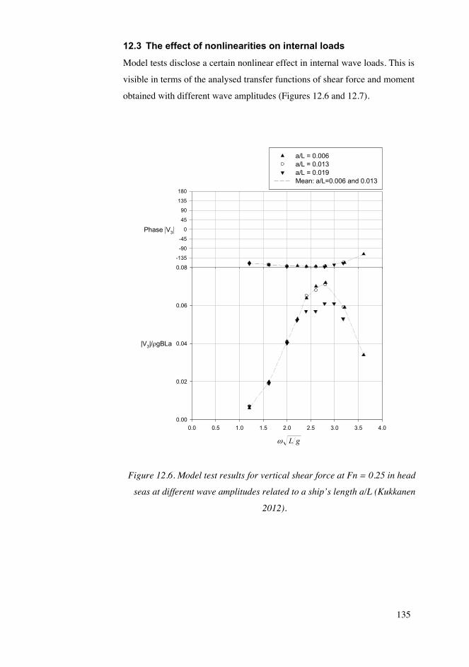
135
12.3 The effect of nonlinearities on internal loads
Model tests disclose a certain nonlinear effect in internal wave loads. This is
visible in terms of the analysed transfer functions of shear force and moment
obtained with different wave amplitudes (Figures 12.6 and 12.7).
Figure 12.6. Model test results for vertical shear force at Fn = 0.25 in head
seas at different wave amplitudes related to a ship’s length a/L (Kukkanen
2012).
0.0 0.5 1.0 1.5 2.0 2.5 3.0 3.5 4.0
|V3|/ρgBLa
0.00
0.02
0.04
0.06
0.08
a/L = 0.006a/L = 0.013a/L = 0.019Mean: a/L=0.006 and 0.013
Phase |V3|
-135
-90
-45
0
45
90
135
180
gLω

136
Figure 12.7. Model test results for bending moment (right-V5) at Fn = 0.25 in
head seas at different wave amplitudes related to a ship’s length a/L
(Kukkanen 2012).
The nonlinearities are visible as differing values of RAOs for the
frequencies close to resonance obtained with different wave amplitudes
(denoted by small letter a in the Figure 12.6).
Kukkanen (2012) has investigated the effect of nonlinearities of wave
induced motion and internal loads of the RoPax ship presented above. He
has studied this subject with the dedicated model tests conducted in the
towing tank at Aalto University and with the theoretical model. The latter is
based on a Green function representation of the velocity potential of a time-
domain flow with a free surface (GFM) and allows for the most important
0.0 0.5 1.0 1.5 2.0 2.5 3.0 3.5 4.0
|V5|/ρgBL2a
0.000
0.005
0.010
0.015
0.020
0.025
0.030
a/L = 0.006a/L = 0.013a/L = 0.019Mean: a/L=0.006 and 0.013
Phase |V5|
-135
-90
-45
0
45
90
135
180
gLω

137
nonlinearities of wave loads. Both, the experiments and the computations
reveal un-symmetry of internal loads, resulting in different maximum values
in sagging and hogging conditions. This is shown in figures 12.8, 12.9,
12.10 and 12.11 below.
Figure 12.8 Maximum and minimum peaks of the shear force at Fn = 0.0.
Calculation was carried out with the relative wave amplitude a/L = 0.013
using the body nonlinear and the body-wave nonlinear solutions.
0.0 0.5 1.0 1.5 2.0 2.5 3.0 3.5 4.0
V3/ρgBLa
-0.08
-0.06
-0.04
-0.02
0.00
0.02
0.04
0.06
0.08
Model tests Body and wave nonlin.Body nonlin.
gLω

138
Figure 12.9 Maximum and minimum peaks of bending moment at Fn = 0.0.
Calculation was carried out with the relative wave amplitude a/L = 0.013
using the body nonlinear and the body-wave nonlinear solutions.
Figure 12.10 Maximum and minimum peaks of the shear at Fn = 0.25.
Calculation was carried out with the relative wave amplitude a/L = 0.013
using the body nonlinear and the body-wave nonlinear solutions.
0.0 0.5 1.0 1.5 2.0 2.5 3.0 3.5 4.0
V5/ρgBL2a
-0.030
-0.020
-0.010
0.000
0.010
0.020
0.030
Model tests Body and wave nonlin.Body nonlin.
gLω
0.0 0.5 1.0 1.5 2.0 2.5 3.0 3.5 4.0
V3/ρgBLa
-0.10
-0.05
0.00
0.05
0.10 Model tests Body and wave nonlin.Body nonlin.
gLω

139
Figure 12.11 Maximum and minimum peaks of the bending at Fn = 0.25.
Calculation was carried out with the relative wave amplitude a/L = 0.013
using the body nonlinear and the body-wave nonlinear solutions.
There is a clear difference in sagging and hogging maximum values of
internal loads. The shear force at the ship’s forepart and the bending
moment at the mid-ship are significantly higher for the sagging condition.
The bow flare, flat bottom at stern and load caused by the steady wave
generated by hull at speed are the main contributors to this un-symmetry.
0.0 0.5 1.0 1.5 2.0 2.5 3.0 3.5 4.0
V5/ρgBL2a
-0.040
-0.020
0.000
0.020
0.040
Model tests Body and wave nonlin.Body nonlin.
gLω

140
References
Bertram, V. 2000 Practical Ship Hydrodynamics, Butterworth-Heinemann, ISBN 0 7506 4851 1.
Brix, J. 1993 Manoeuvring Technical Manual, Seehafen Verlag GmbH, Hamburg
Clayton B. R. & Bishop, R.E.D. 1982 Mechanics of Marine Vehicles, London, ISBN 0 419 12110-2.
Cummins, W.E. 1962. The impulse response function and ship motions. Schiffstechnik pp. 101–109.
Faltinsen, O. M. 1990. Sea Loads on Ships and Offshore Structures, Cambridge University Press, 328 p.
Fossen, T. I. 1994. Guidance And Control Of Ocean Vehicles, J. Wiley&Sons, ISBN 0 471 94113 1.
Garrison, C. J. 1974. Dynamic response of floating bodies. Houston. Proceedings in Offshore Technology Conference, paper No. 2067, pp. 365 – 377.
Matusiak, J. 2000. Dynamics of cargo shift onboard a ship in irregular beam waves, International Shipbuilding Progress, 47, No 449 pp. 77-93
Hamamoto, M. & Kim, Y.S. 1993. A New Coordinate System and the Equations Describing Manoeuvring Motion of a Ship in Waves, J. Soc. Naval Arch., Vol 173.
IMO i.e. International Maritime Organization, SLF 49/5 Revised Intact Stability Code prepared by the Intersessional Correspondence Group.
International Maritime Organization, 2008. SLF 49/WP.2 ANNEX 2, Revised Guidance to the Master for Avoidance Dangerous Situations in Adverse Weather and Sea Conditions.
Ischida, S. et al, 2006. Evaluation of the weather criterion by experiments and its effect to the design of a RoPax ferry. In Proceedings of the 9th International Conference on Stability of Ships and Ocean Vehicles, STAB 2006, 25-29 September, 2006, Rio de Janeiro, Brazil.

141
Journee J. M. 1992. Strip Theory Algorithms, report MEMT 24, Delft University of Technology, Ship Hydrodynamics Laboratory.
Kreyshig, E. 1993. Advanced Engineering Mathematics. John Wiley&Sons, Inc. 7th edition.
Kukkanen, T. 2012. Numerical and experimental studies of nonlinear wave loads of ships, doctoral dissertation, VTT Science 15.
23rd International Towing Tank Conference, 2002. Report of the Specialist Committee of Extreme Ship Motions and Capsizing, Venice Italy, September 8-14, 2002, in Proceedings of the Conference, Vol. 2.
Lloyd, A.R.J.M, 1989. Seakeeping: Ship Behaviour in Rough Weather, Ellis Horwood Ltd.
Luukkainen, Niilo 2011. Modelling of Hydrodynamic Phenomena in Simulation of Ship Manoeuvring, Aalto University, School of Engineering, Department of Applied Mechanics, Master Thesis (in Finnish).
Mattila, M. 1999. An investigation of the dynamic stability of a fast RoPax vessel in waves (in Finnish), Helsinki University of Technology, Mechanical Engineering Department, Master Thesis.
Matusiak, J. 1995. Ship Buoyancy and Stability. Otatieto Oy. Helsinki 1995 (textbook in Finnish).
Matusiak, J. 2000. Dynamics of cargo shift onboard a ship in irregular beam waves, International Shipbuilding Progress, 47, No 449 pp. 77-93.
Matusiak, Jerzy 2003. On the effects of wave amplitude, damping and initial conditions on the parametric roll resonance. Proceedings of the 8th International Conference on Stability of Ships and Ocean Vehicles, Madrid, Spain, September 2003, pp. 341-348.
Matusiak, Jerzy 2003. Momentum equation applied to the problem of a propeller in oblique flow. Ship Technology Research-Schiffstechnik, Vol. 50-2003, pp. 103-105.
Matusiak, J. 2005. Ship Propulsion. Helsinki University of Technology. Ship Laboratory. Report M-176. Otaniemi 2005. Sixth edition. (in Finnish).
Matusiak, Jerzy; Hamberg, Karl, 2006. Considerations on the weather criterion applicability for the stability assessment of the large vessels. In Proceedings of the 9th International

142
Conference on Stability of Ships and Ocean Vehicles, Rio de Janeiro, Brasilia, 25.-29.9.2006. 447-454 (Vol 1).
Molland, A.F. &Turnock, S.R. 2007. Marine Rudders and Control Surfaces Elsevier Ltd. ISBN978-0.75-0-066944-3.
Naito, S. 1995. Generation and absorption of waves. Symposium on Wave Generation, Analysis and Related Problems in Experimental Tanks- Especially on Directional Wave. Yokohama National University, 25 September 1995. Pp. 1-27.
Newman, J.N. 1980. Marine Hydrodynamics. Cambridge, Massachusetts, The MIT Press, 402 s. Washington, D.C 1997.
Ohkusu, M. editor 1996. Advances in Marine Hydrodynamics, Computational Mechanics Publications, Southampton Boston.
Ruponen, Pekka 2004. Calculation Method for the Steering Forces of a Pod in Hybrid Propulsion. Master Thesis, Faculty of Mechanical Engineering, Helsinki University of Technology, in Finnish.
Ruponen, Pekka; Matusiak, Jerzy 2004. Calculation Method for the Steering Forces of a Pod in Hybrid Propulsion. First International Conference on Technological Advances in Podded Propulsion, Newcastle, 14.-16.4.2004. 2004, University of Newcastle, 263-275.
Salonen, E-M., 1999. Dynamiikka II. Otakustantamo 591 (in Finnish).
Söding, H. 1982. Prediction of ship steering capabilities, Schiffstechnik, Band 29, Heft 1, März 1982 pp. 3-29.
Stigler, C. 2012. Investigation of the behaviour of a RoPax vessel in stern quartering irregular long-crested waves, Student research project (Aalto University&Hamburg University of Technology.
Triantafyllou Michael S. & Hover Franz S. 2003. Manoeuvring and control of marine vehicles, Department of Ocean Engineering, Massachusetts Institute of Technology, Cambridge, Massachusetts USA.
Yoon, Hyeon Kyu et al, 2006. Application and Review on Interim Guidelines for Alternative Assessment of the Weather Criterion. In Proceedings of the 9th International Conference on Stability of Ships and Ocean Vehicles, STAB 2006, 25-29 September, 2006, Rio de Janeiro, Brazil.

143
Young, Ian R. 2000. Wind generated ocean waves, Amsterdam, 2000. Elsevier ocean engineering book series; 2 ISBN 0-08-043317-0.

144
Appendix A. Co-ordinate
systems used in the context of the linear seakeeping theory
In the linear seakeeping theory and in manoeuvring normally three co-
ordinate systems fixed with ship are considered. They are all right-handed
systems and their origins are located at the symmetry plane of the ship. The
z-axes of two of the systems are passing through the centre of gravity of
ship G. In the manoeuvring the most common approach is to have motion
and forces expressed in the co-ordinate system xM,yM,zM, with the origin
located at the vertical encompassing centre of gravity G and at the still water
plane (Journee 1992). The vertically oriented zM-axis points upwards.
Another co-ordinate system used in this work, x,y,z is located at the centre
of gravity of ship G and the z-axis is oriented downwards. The third co-
ordinate system, the so-called Tasai’s co-ordinate system, has an origin
located at the water plane and at mid-ship. The co-ordinates systems are
shown in Figure A.1 below.

145
Fig. A.1 Co-ordinate systems.
The distance of the centre of gravity G from the water-plane is marked by
zG. The longitudinal (that is, the x-directional distance) of the origins is
denoted by xG.
Ship motions in terms of displacements are depicted as the co-ordinates.
Angular motions are marked as φ0, θ0, ψ0 and φ, θ, ψ. These are small
angular motions in the co-ordinate systems x0,y0,z0 and x,y,z respectively.
The relation between the motion components, forces and moments in these
two co-ordinate systems are as follows
x = x0 + zGθ0, y = −y0 + zGφ0 − xGψ0, z = −z0 + xGθ0
φ = φ0, θ =−θ0, ψ =−ψ0
X = X0, Y = −Y0, Z = −Z0
K = K0 + zGY0, M = −M0 + zGX0 − xGZ0, N = −N0 + xGY0. (A.1)
Equations A.1 can be written in a matrix form as follows

146
x{ } =
xyzφθψ
⎧
⎨
⎪⎪⎪
⎩
⎪⎪⎪
⎫
⎬
⎪⎪⎪
⎭
⎪⎪⎪
= T1[ ] x0{ } =
1 0 0 0 zG 00 −1 0 zG 0 −xG0 0 −1 0 xG 00 0 0 1 0 00 0 0 0 −1 00 0 0 0 0 −1
⎡
⎣
⎢⎢⎢⎢⎢⎢
⎤
⎦
⎥⎥⎥⎥⎥⎥
x0y0z0φ0θ0ψ0
⎧
⎨
⎪⎪⎪
⎩
⎪⎪⎪
⎫
⎬
⎪⎪⎪
⎭
⎪⎪⎪
X{ } =
XYZKMN
⎧
⎨
⎪⎪
⎩
⎪⎪
⎫
⎬
⎪⎪
⎭
⎪⎪
= T2[ ] X0{ } =
1 0 0 0 0 00 −1 0 0 0 00 0 −1 0 0 00 zG 0 1 0 0zG 0 −xG 0 −1 00 xG 0 0 0 −1
⎡
⎣
⎢⎢⎢⎢⎢⎢
⎤
⎦
⎥⎥⎥⎥⎥⎥
X0Y0Z0K0
M 0
N0
⎧
⎨
⎪⎪⎪
⎩
⎪⎪⎪
⎫
⎬
⎪⎪⎪
⎭
⎪⎪⎪
(A.2)
Linear strip seakeeping theory yields the radiation forces expressed with the
aid of added masses Aij and damping Bij coefficients in the x0,y0,z0 co-
ordinate system and as dependent upon the acceleration and velocities in the
following form
X0{ }=
X0
Y0
Z0
K0
M 0
N0
⎧
⎨
⎪⎪⎪
⎩
⎪⎪⎪
⎫
⎬
⎪⎪⎪
⎭
⎪⎪⎪
=− A[ ] x0{ }− B[ ] x0{ } =−
A11 0 0 0 0 00 A22 0 A24 0 A26
0 0 A33 0 A35 00 0 0 A44 0 A46
0 0 A35 0 A55 00 A26 0 A46 0 A66
⎡
⎣
⎢⎢⎢⎢⎢⎢
⎤
⎦
⎥⎥⎥⎥⎥⎥
x0
y0
z0
φ0
θ0
ψ0
⎧
⎨
⎪⎪⎪
⎩
⎪⎪⎪
⎫
⎬
⎪⎪⎪
⎭
⎪⎪⎪
−
B11 0 0 0 0 00 B22 0 B24 0 B26
0 0 B33 0 B35 00 B24 0 B44 0 B46
0 0 B35 0 B55 00 B26 0 B46 0 B66
⎡
⎣
⎢⎢⎢⎢⎢⎢
⎤
⎦
⎥⎥⎥⎥⎥⎥
x0
y0
z0
φ0
θ0
ψ0
⎧
⎨
⎪⎪⎪
⎩
⎪⎪⎪
⎫
⎬
⎪⎪⎪
⎭
⎪⎪⎪
(A.3)
Added masses and damping coefficients in the x,y,z co-ordinate system
Added mass and damping matrices are needed in the equations of motions
set with the ship’s origin located in the centre of gravity and with the co-
ordinates fixed with a ship (axes x,y,z). For this reason matrices [A] and [B]
have to be transferred to the x,y,z co-ordinate system having the origin in the
ship’s centre of gravity. This is done as follows. Using the first of relations
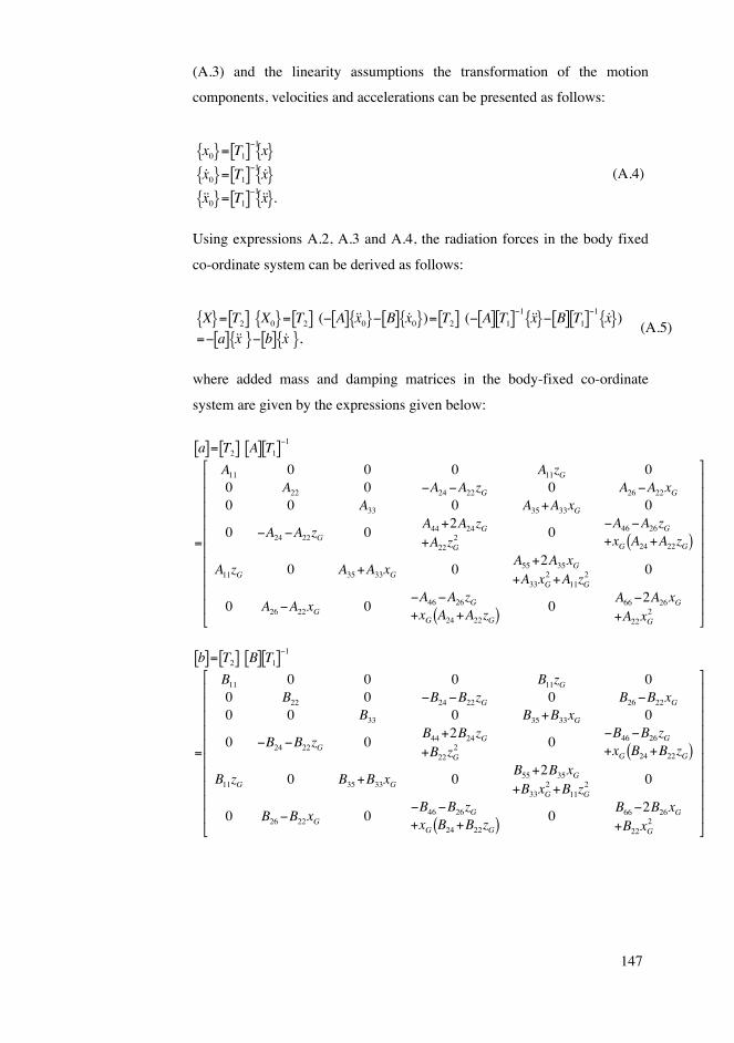
147
(A.3) and the linearity assumptions the transformation of the motion
components, velocities and accelerations can be presented as follows:
x0{ }= T1[ ]−1 x{ }x0{ }= T1[ ]−1 x{ }x0{ }= T1[ ]−1 x{ }.
(A.4)
Using expressions A.2, A.3 and A.4, the radiation forces in the body fixed
co-ordinate system can be derived as follows:
X{ }= T2[ ] X0{ }= T2[ ] (− A[ ] x0{ }− B[ ] x0{ })= T2[ ] (− A[ ] T1[ ]−1 x{ }− B[ ] T1[ ]−1 x{ })=− a[ ] x{ }− b[ ] x{ },
(A.5)
where added mass and damping matrices in the body-fixed co-ordinate
system are given by the expressions given below:
a[ ]= T2[ ] A[ ] T1[ ]−1
=
A11 0 0 0 A11zG 00 A22 0 −A24 −A22zG 0 A26−A22xG0 0 A33 0 A35+A33xG 0
0 −A24 −A22zG 0A44+2A24zG+A22zG
2 0−A46−A26zG+xG A24+A22zG( )
A11zG 0 A35+A33xG 0A55+2A35xG+A33xG
2 +A11zG2 0
0 A26−A22xG 0−A46−A26zG+xG A24+A22zG( ) 0
A66−2A26xG+A22xG
2
⎡
⎣
⎢⎢⎢⎢⎢⎢⎢⎢⎢⎢
⎤
⎦
⎥⎥⎥⎥⎥⎥⎥⎥⎥⎥
b[ ]= T2[ ] B[ ] T1[ ]−1
=
B11 0 0 0 B11zG 00 B22 0 −B24 −B22zG 0 B26−B22xG0 0 B33 0 B35+B33xG 0
0 −B24 −B22zG 0B44+2B24zG+B22zG
2 0−B46−B26zG+xG B24+B22zG( )
B11zG 0 B35+B33xG 0B55+2B35xG+B33xG
2 +B11zG2 0
0 B26−B22xG 0−B46−B26zG+xG B24+B22zG( ) 0
B66−2B26xG+B22xG
2
⎡
⎣
⎢⎢⎢⎢⎢⎢⎢⎢⎢⎢
⎤
⎦
⎥⎥⎥⎥⎥⎥⎥⎥⎥⎥

148
Appendix B Cosine transform
using FFT
Transformation of the added masses from the frequency to time domain
involves an evaluation of the integral
Kij (t)=
2
πBij (ω)cos(ωt)dω
0
ωmax
∫ . (B.1)
This integral is called retardation or memory function. It can be
approximated by the sum
Kk ,ij (kΔt)=
2
πBij (rΔω)
r=0
N−1
∑ cos(rΔωkΔt)Δω. (B.2)
Selecting the frequency and time spacing is as follows. Time increment Δt is
selected. It is the same as the time step used in the numerical integration of
the equations of motion. The integer number N=2n is selected and the
maximum angular frequency and frequency increament used in the Fast-
Fourier-Transform (FFT) analysis are evaluated from:
ωmax = 2π / ΔtΔω =ωmax / N . (B.3)
yields
Kk ,ij (kΔt)=
2Δωπ
Bij (rΔω)r=0
N−1
∑ cos(2πrk / N ). (B.4)
Expression B.4 can be evaluated using the FFT algorithm as follows
Kk ,ij (kΔt)=
NΔωπ
FFT(gij (x)), (B.5)
where the original added damping discrete functions are substituted by a
‘double-sided function’ g(x) as follows:
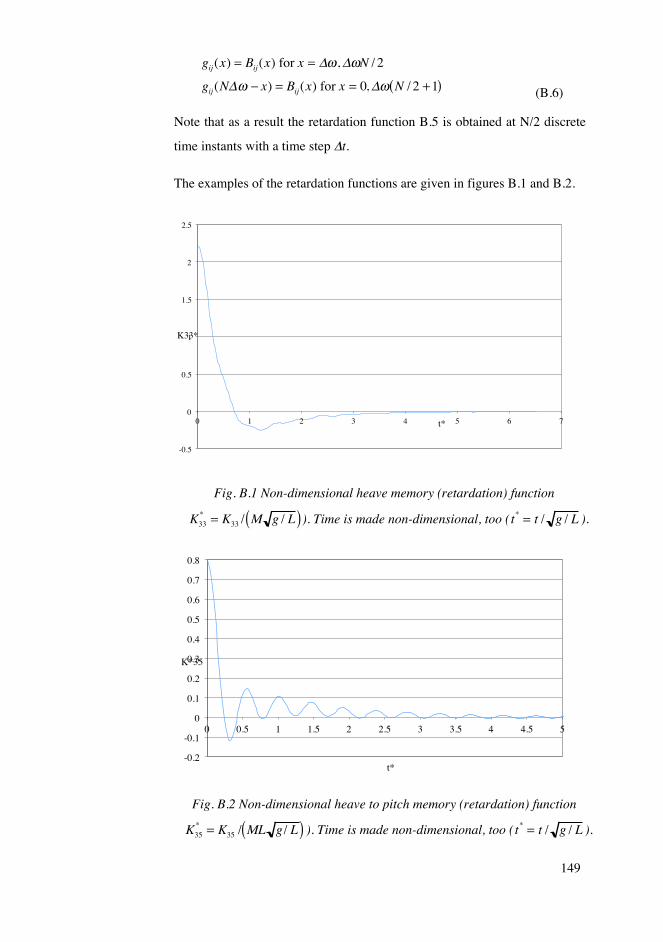
149
gij(x) = Bij(x) for x = Δω,ΔωN / 2
gij(NΔω − x) = Bij(x) for x = 0,Δω N / 2 +1( ) (B.6)
Note that as a result the retardation function B.5 is obtained at N/2 discrete
time instants with a time step Δt.
The examples of the retardation functions are given in figures B.1 and B.2.
Fig. B.1 Non-dimensional heave memory (retardation) function
K33* = K33 / M g / L( )). Time is made non-dimensional, too (t* = t / g / L ).
Fig. B.2 Non-dimensional heave to pitch memory (retardation) function
K35* = K35 / ML g/ L( ) ). Time is made non-dimensional, too ( t* = t / g / L ).
-0.5
0
0.5
1
1.5
2
2.5
0 1 2 3 4 5 6 7
K33*
t*
-0.2
-0.1
0
0.1
0.2
0.3
0.4
0.5
0.6
0.7
0.8
0 0.5 1 1.5 2 2.5 3 3.5 4 4.5 5
K*35
t*

NBSI 3-2627-06-259-879 )fdp( L-NSSI 6984-9971
NSSI 6984-9971 )detnirp( NSSI X094-9971 )fdp(
ytisrevinU otlaA
gnireenignE fo loohcS gnireenignE lacinahceM fo tnemtrapeD
if.otlaa.www
+ SSENISUB YMONOCE
+ TRA
+ NGISED ERUTCETIHCRA
+ ECNEICS
YGOLONHCET
REVOSSORC
LAROTCOD SNOITATRESSID
-otl
aA
TS
2/
710
2
kai
suta
M yz
reJ
pih
S di
giR
a fo
sci
many
D y
tisr
evi
nU
otla
A
7102
gnireenignE lacinahceM fo tnemtrapeD
kaisutaM yzreJ
LAIRETAM GNINRAEL + ECNEICS YGOLONHCET
pihS digiR a fo scimanyD