dynamic optimization with random and …dc800dx8184/thesis...family including my wife heather, my...
TRANSCRIPT

DYNAMIC OPTIMIZATION
WITH RANDOM AND SMOOTHED CONSTRAINTS
A DISSERTATION
SUBMITTED TO THE DEPARTMENT OF ELECTRICAL
ENGINEERING
AND THE COMMITTEE ON GRADUATE STUDIES
OF STANFORD UNIVERSITY
IN PARTIAL FULFILLMENT OF THE REQUIREMENTS
FOR THE DEGREE OF
DOCTOR OF PHILOSOPHY
Ekine Omoni Akuiyibo
August 2011
http://creativecommons.org/licenses/by-nc/3.0/us/
This dissertation is online at: http://purl.stanford.edu/dc800dx8184
© 2011 by Ekine Akuiyibo. All Rights Reserved.
Re-distributed by Stanford University under license with the author.
This work is licensed under a Creative Commons Attribution-Noncommercial 3.0 United States License.
ii

I certify that I have read this dissertation and that, in my opinion, it is fully adequatein scope and quality as a dissertation for the degree of Doctor of Philosophy.
Stephen Boyd, Primary Adviser
I certify that I have read this dissertation and that, in my opinion, it is fully adequatein scope and quality as a dissertation for the degree of Doctor of Philosophy.
John Gill, III, Co-Adviser
I certify that I have read this dissertation and that, in my opinion, it is fully adequatein scope and quality as a dissertation for the degree of Doctor of Philosophy.
Daniel O'Neill
Approved for the Stanford University Committee on Graduate Studies.
Patricia J. Gumport, Vice Provost Graduate Education
This signature page was generated electronically upon submission of this dissertation in electronic format. An original signed hard copy of the signature page is on file inUniversity Archives.
iii

Abstract
Stochastic control theory is a well known mathematical framework that is widely ap-
plied because of its robustness. This thesis describes the use of stochastic control,
convex optimization, and time smoothing, for resource allocation in radio communi-
cation systems.
Radio systems are inherently complex due to randomness in the propagation
medium, i.e., wireless channels, caused by fading, interference from participatory
devices, device mobility, etc. As the demand for heterogeneous multimedia services
increases, it has become increasingly important to devise more efficient resource allo-
cation strategies. These resource allocation problems can be represented as network
flow control problems where the goal is to design flow controllers, which are equivalent
to network protocols. Over the years, adaptive controllers have been proposed and
implemented to replace less efficient static controllers. Unfortunately, most current
adaptive schemes are complicated and largely heuristic.
We present a stochastic control framework, that integrates adaptive modulation
and network utility maximization, for designing simple and implementable adaptive
flow rate controllers for efficient and fair resource allocation. For each problem pre-
sented, we first characterize the exact optimal controller and in a few special cases we
show how to compute this optimal controller. For cases where computing the optimal
controller is intractable, we design efficient suboptimal controllers using approximate
dynamic programming.
iv
In the first problem we look at a resource allocation problem with random affine
resource constraints. Using quadratic stage costs, this problem reduces to a varia-
tion on (affine) linear quadratic regulation where the resulting flow rate controller
is an affine function of the system state and the random resources. In the second
problem, we design flow rate controllers to optimally tradeoff average transmit power
and average utility of smoothed flows on a single time-varying wireless link. The
smoothing takes into account the heterogeneous time profiles of different applications
in the dynamic environment, producing significantly different control policies. Lastly,
in the third problem, we design multi-link flow rate controllers that optimally tradeoff
average flow utility, average transmit power, and average queue maintenance costs.
We derive interesting queue-length-based metrics associated with different utility and
cost functions.
v
Acknowledgments
This thesis is the culmination of works made possible by the help and support of
several people.
First, I would like to thank my advisor, Prof. Stephen Boyd, for his unwavering
support and encouragement throughout my time in his research group. His seemingly
effortless brilliance, clarity, and simplicity, I know now to be a result of his strong
passion for teaching. I continue to incorporate these tenets in my own work.
I would like to thank Prof. Daniel O’Neill for the several discussions we had about
application of my work to wireless communications. His suggestions were central to
the problems we investigated.
I would like to thank Prof. Kunle Olukotun for chairing my orals committee and
Prof. John Gill for being a member of my orals and reading committees. Many thanks
to Prof. Brad Osgood and Dr. Noe Lozano for enabling me secure initial funding to
come to Stanford — their support over the years encompasses much more. Thanks
to Prof. Abbas El Gamal for introducing me to Dr. Olivier Lévêque. The work
with Olivier and Prof. Emre Telatar at École Polytechnique Fédérale de Lausanne
reinvigorated my research curiosity.
I would like to thank current and former members of my research group, Arezou,
Argyrios, Borja, Brendan, (cvx, Michael), Eric, Ivan, Joëlle, Joseph, Kwangmoo,
Matt, and Neal. It has been a pleasure to learn from, and work with you, these last
few years.
vi
Special thanks to Jacob, Tosin, and Yang, for the numerous extra sessions — your
checks are in the mail!
Finally, I have been blessed with the constant love and support from my incredible
family including my wife Heather, my parents, Deaconess (Dr.) Ibiere Akuiyibo and
Dr. Dimabo Akuiyibo, my siblings, Owualata, Kuraye, Dumo, Preye, my parents-in-
law, Helen and Scott, and my nephews, Carl and Daniel. This accomplishment is ours
to share. I am especially grateful to Heather for her patience, her daily encouragement
and cheerful disposition, and for having the kindest heart imaginable.
Mom and Dad permitted me to aspire — this thesis is dedicated to them.
vii
Contents
Abstract iv
Acknowledgments vi
1 Overview 1
1.1 Outline . . . . . . . . . . . . . . . . . . . . . . . . . . . . . . . . . . . 1
1.2 Notation . . . . . . . . . . . . . . . . . . . . . . . . . . . . . . . . . . 3
2 Stochastic Control with Random Resource Constraints 4
2.1 Problem statement . . . . . . . . . . . . . . . . . . . . . . . . . . . . 4
2.2 Results . . . . . . . . . . . . . . . . . . . . . . . . . . . . . . . . . . . 7
2.3 Optimal policy via dynamic programming . . . . . . . . . . . . . . . 8
2.4 Evaluating the Bellman operator . . . . . . . . . . . . . . . . . . . . 10
2.5 Numerical example . . . . . . . . . . . . . . . . . . . . . . . . . . . . 14
2.6 Conclusion . . . . . . . . . . . . . . . . . . . . . . . . . . . . . . . . . 15
3 Adaptive Modulation with Smoothed Flow Utility 22
3.1 Background . . . . . . . . . . . . . . . . . . . . . . . . . . . . . . . . 23
3.2 Problem setup . . . . . . . . . . . . . . . . . . . . . . . . . . . . . . . 23
3.3 Optimal policy characterization . . . . . . . . . . . . . . . . . . . . . 29
3.4 Single flow case . . . . . . . . . . . . . . . . . . . . . . . . . . . . . . 38
viii
3.5 A suboptimal policy for the multiple flow case . . . . . . . . . . . . . 45
3.6 Upper bound policies . . . . . . . . . . . . . . . . . . . . . . . . . . . 50
3.7 Other concave utilities . . . . . . . . . . . . . . . . . . . . . . . . . . 55
3.8 Alternative evaluation of ADP policy . . . . . . . . . . . . . . . . . . 63
3.9 Conclusion . . . . . . . . . . . . . . . . . . . . . . . . . . . . . . . . . 70
4 Queue-Length-Based 2-Hop Rate Control 72
4.1 Background . . . . . . . . . . . . . . . . . . . . . . . . . . . . . . . . 72
4.2 Network description . . . . . . . . . . . . . . . . . . . . . . . . . . . . 73
4.3 Optimal policy . . . . . . . . . . . . . . . . . . . . . . . . . . . . . . 77
4.4 One flow . . . . . . . . . . . . . . . . . . . . . . . . . . . . . . . . . . 79
4.5 Numerical Examples . . . . . . . . . . . . . . . . . . . . . . . . . . . 80
4.6 Queue metrics . . . . . . . . . . . . . . . . . . . . . . . . . . . . . . . 89
4.7 Multiple flows . . . . . . . . . . . . . . . . . . . . . . . . . . . . . . . 94
4.8 Conclusion . . . . . . . . . . . . . . . . . . . . . . . . . . . . . . . . . 95
Bibliography 96
ix
List of Figures
2.1 Sample flow allocation trajectories, optimal policy (red), equal sharing
policy (blue). . . . . . . . . . . . . . . . . . . . . . . . . . . . . . . . 16
2.2 Sample utility state trajectories, optimal policy (red), equal sharing
policy (blue). . . . . . . . . . . . . . . . . . . . . . . . . . . . . . . . 17
2.3 Error histograms for flow 1. Top. Absolute difference between the
optimal policy utility state and target utility state. Bottom. Absolute
difference between the equal sharing utility state and target utility state. 18
2.4 Error histograms for flow 2. Top. Absolute difference between the
optimal policy utility state and target utility state. Bottom. Absolute
difference between the equal sharing utility state and target utility state. 19
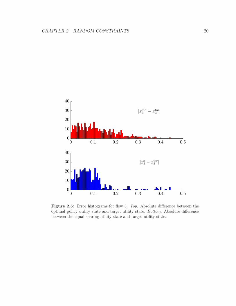
2.5 Error histograms for flow 3. Top. Absolute difference between the
optimal policy utility state and target utility state. Bottom. Absolute
difference between the equal sharing utility state and target utility state. 20
3.1 Value functions for T = 1, 5, 10, 20, 25, 50. . . . . . . . . . . . . . . . . 35
3.2 Value functions for α = 1/10, 1/3, 1/2, 2/3, 3/4. . . . . . . . . . . . . 36
3.3 Top. Comparing V (blue) with V (red, dashed) for the lightly smoothed
flow. Bottom. Comparing V (blue) with V (red, dashed) for the heav-
ily smoothed flow. . . . . . . . . . . . . . . . . . . . . . . . . . . . . . 41
x
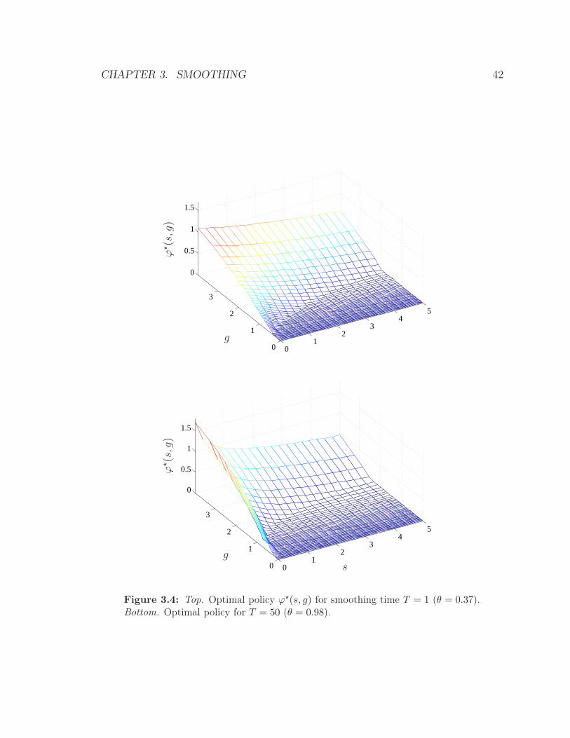
3.4 Top. Optimal policy ϕ⋆(s, g) for smoothing time T = 1 (θ = 0.37).
Bottom. Optimal policy for T = 50 (θ = 0.98). . . . . . . . . . . . . . 42
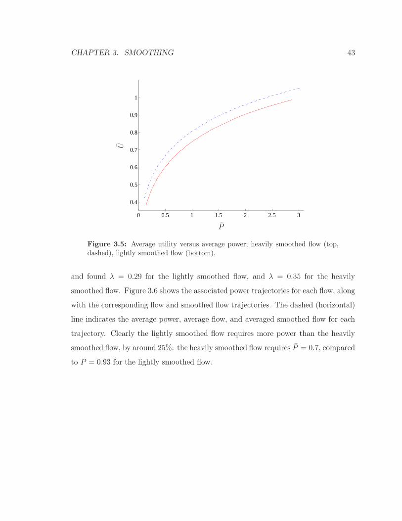
3.5 Average utility versus average power; heavily smoothed flow (top, dashed),
lightly smoothed flow (bottom). . . . . . . . . . . . . . . . . . . . . . 43
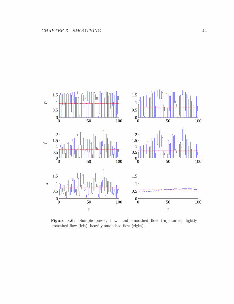
3.6 Sample power, flow, and smoothed flow trajectories; lightly smoothed
flow (left), heavily smoothed flow (right). . . . . . . . . . . . . . . . . 44
3.7 ADP controllers for 200 values in λ ∈ [0.5, 10]. . . . . . . . . . . . . . 50
3.8 Prescient bound (blue), ADP controller (red), for λ = 0.5, infeasible
controller region (shaded). . . . . . . . . . . . . . . . . . . . . . . . . 53
3.9 Prescient bound (blue), ADP controllers (red), for λ = {0.5, 1}, infea-
sible controller region (shaded). . . . . . . . . . . . . . . . . . . . . . 54
3.10 Prescient bound (blue), ADP controller (red), for λ = {0.5, 1, 1.5},
infeasible controller region (shaded). . . . . . . . . . . . . . . . . . . . 54
3.11 Prescient bound (blue), ADP controllers (red), for 200 values of λ ∈
[0.5, 10], infeasible controller region (shaded). . . . . . . . . . . . . . . 55
3.12 Top. Comparing V (blue) with V (red, dashed) for the lightly smoothed
flow. Bottom. Comparing V (blue) with V (red, dashed) for the heav-
ily smoothed flow. . . . . . . . . . . . . . . . . . . . . . . . . . . . . . 57
3.13 Top. Optimal policy ϕ⋆(s, g) for smoothing time T = 1 (θ = 0.37).
Bottom. Optimal policy for T = 100 (θ = 0.99). . . . . . . . . . . . . 58
3.14 Top. Optimal policy level curves for T = 1 (θ = 0.37). Bottom.
Optimal policy level curves for T = 100 (θ = 0.99). . . . . . . . . . . 59
3.15 Top. Log utility average utility versus average power. Bottom. Log
utility average utility U = −1.5 versus average power. . . . . . . . . . 60
3.16 Top. Log utility sample power trajectory for lightly smoothed flow.
Bottom. Log utility sample power trajectory for heavily smoothed flow. 61
3.17 Saturated linear utility functions: U0.5,0.375, U1,1, U2,0.5. . . . . . . . . 62
xi
3.18 Top. Value function and power-law approximate for U1,1(s) and T = 1.
Bottom. Value function and power-law approximate for U1,1(s) and
T = 50. . . . . . . . . . . . . . . . . . . . . . . . . . . . . . . . . . . 64
3.19 Top. Power law policy ϕ⋆(s, g) for U1,1(s) and smoothing time T = 1
(θ = 0.37). Bottom. Policy law policy for U1,1(s) and T = 50 (θ = 0.98). 65
3.20 Top. Saturated linear U1,1 tradeoff curves for T = 1, 50. Bottom.
Power, flow and smoothed flow trajectories. . . . . . . . . . . . . . . 66
4.1 Single-hop network. . . . . . . . . . . . . . . . . . . . . . . . . . . . . 73
4.2 Single hop, single flow. . . . . . . . . . . . . . . . . . . . . . . . . . . 79
4.3 Comparing optimal value function (blue) with approximate value func-
tion (red, dashed). χ(q) = 0.5q2. Vmax = 0.32, qmax = 0.31, qzero =
0.73. . . . . . . . . . . . . . . . . . . . . . . . . . . . . . . . . . . . . 83
4.4 Top. Sample flow 1 trajectory. Middle. Sample queue length trajec-
tory. Bottom. Sample flow 2 trajectory. χ(q) = 0.5q2. . . . . . . . . . 84
4.5 Comparing optimal value function (blue) with approximate value func-
tion (red, dashed). χ(q) = 0.5q2. Vmax = 0.17, qmax = 0.13, qzero =
0.43. . . . . . . . . . . . . . . . . . . . . . . . . . . . . . . . . . . . . 85
4.6 Top. Sample flow 1 trajectory. Middle. Sample queue length trajec-
tory. Bottom. Sample flow 2 trajectory. χ(q) = 0.5q2. . . . . . . . . . 86
4.7 Comparing objective versus weighted queue maintenance cost. Quadratic
queue maintenance cost (red), linear queue maintenance cost (blue). . 87
4.8 Average service rate versus average queueing delay. Quadratic costs
(red, dashed), linear costs (blue). . . . . . . . . . . . . . . . . . . . . 91
4.9 Average service rate versus overall objective J . Quadratic costs (red,
dashed), linear costs (blue). . . . . . . . . . . . . . . . . . . . . . . . 92
xii
4.10 Average arrival rate versus average queue-length. Quadratic costs (red,
dashed), linear costs (blue). . . . . . . . . . . . . . . . . . . . . . . . 93
4.11 Average service rate versus average queue-length. Quadratic costs (red,
dashed), linear costs (blue). . . . . . . . . . . . . . . . . . . . . . . . 93
xiii
Chapter 1
Overview
This work develops a mathematical framework for designing flow rate controllers for
resource allocation problems in wireless communication systems. In each chapter
we formulate the problem as a discrete-time stochastic control problem with convex
objective. In all problems, the information pattern (information available at decision
time) includes a random component. We compute an optimal feedback control law
using stochastic dynamic programming for cases with quadratic objective and/or
small system state dimension. In cases with large system state dimension we propose
simple controllers based on approximate dynamic programming.
We outline the thesis in §1.1 giving for each chapter a brief description of the
problem and our results. In §1.2, we describe some basic notation used throughout
the thesis.
1.1 Outline
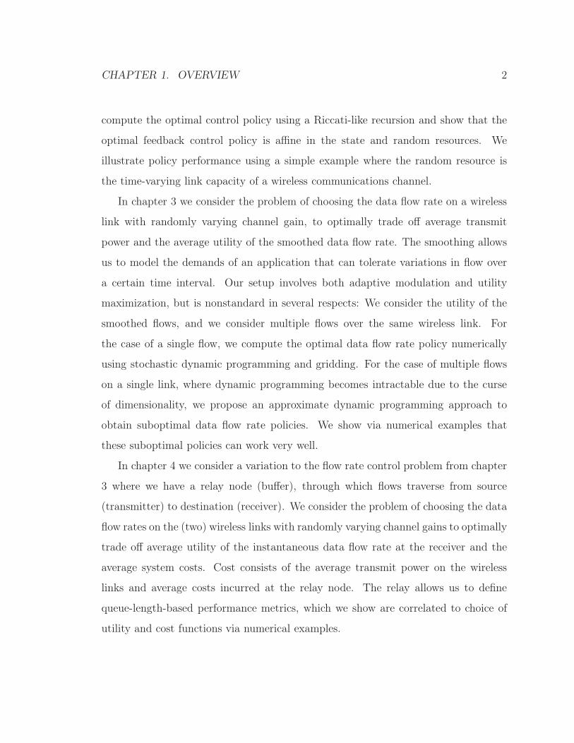
In chapter 2 we consider an infinite-horizon stochastic control problem with quadratic
stage costs and affine constraints. The constraints are functions of random resources
revealed to the controller only in the time period that the constraints apply. We
1
CHAPTER 1. OVERVIEW 2
compute the optimal control policy using a Riccati-like recursion and show that the
optimal feedback control policy is affine in the state and random resources. We
illustrate policy performance using a simple example where the random resource is
the time-varying link capacity of a wireless communications channel.
In chapter 3 we consider the problem of choosing the data flow rate on a wireless
link with randomly varying channel gain, to optimally trade off average transmit
power and the average utility of the smoothed data flow rate. The smoothing allows
us to model the demands of an application that can tolerate variations in flow over
a certain time interval. Our setup involves both adaptive modulation and utility
maximization, but is nonstandard in several respects: We consider the utility of the
smoothed flows, and we consider multiple flows over the same wireless link. For
the case of a single flow, we compute the optimal data flow rate policy numerically
using stochastic dynamic programming and gridding. For the case of multiple flows
on a single link, where dynamic programming becomes intractable due to the curse
of dimensionality, we propose an approximate dynamic programming approach to
obtain suboptimal data flow rate policies. We show via numerical examples that
these suboptimal policies can work very well.
In chapter 4 we consider a variation to the flow rate control problem from chapter
3 where we have a relay node (buffer), through which flows traverse from source
(transmitter) to destination (receiver). We consider the problem of choosing the data
flow rates on the (two) wireless links with randomly varying channel gains to optimally
trade off average utility of the instantaneous data flow rate at the receiver and the
average system costs. Cost consists of the average transmit power on the wireless
links and average costs incurred at the relay node. The relay allows us to define
queue-length-based performance metrics, which we show are correlated to choice of
utility and cost functions via numerical examples.
CHAPTER 1. OVERVIEW 3
1.2 Notation
We use R to denote the set of real numbers. The set of real n-dimensional vectors is
denoted Rn, and the set of real m× n matrices is denoted Rm×n. We delimit vectors
and matrices with square brackets, with the components separated by space. We use
parentheses to construct column vectors from comma separated lists. For example, if
a, b, c ∈ R, we have
(a, b, c) =
a
b
c
= [ a b c ]T ,
which is an element of R3. The symbol 1 denotes a vector all of whose components are
one (with dimension determined from context). We use diag(x1, . . . , xn), or diag(x),
x ∈ Rn, to denote a n× n diagonal matrix with diagonal entries x1, . . . , xn.
The inequality symbol ≥ and its strict form > is used to denote elementwise vector
(or matrix) inequality. The curled inequality symbol � (and its strict form ≻) is used
to denote matrix inequality. For example, for A,B ∈ Rn×n, A � B means that the
matrix A− B is positive semidefinite.
Chapter 2
Stochastic Control with Random
Resource Constraints
We consider a discrete-time stochastic control problem with convex costs and affine
constraints over an infinite time horizon. The constraints are functions of random
resources revealed to the controller only in the time period that the constraints ap-
ply. For the case with quadratic sage costs, we show that we can compute the opti-
mal control policy (and optimal value function) using dynamic programming and a
Riccati-like recursion, and knowing only the first and second moments of the random
resources. We show that the optimal control law is a feedback policy that is affine
in the state and random resources. We illustrate our policy performance using an
example where the random resource is the time-varying capacity of a wireless link.
2.1 Problem statement
System dynamics. Consider the discrete-time linear dynamical system
xt+1 = Axt +But + wt, t = 0, 1, . . . ,
4
CHAPTER 2. RANDOM CONSTRAINTS 5
where xt ∈ Rn denotes the state vector, ut ∈ Rm denotes the input vector, A ∈ Rn×n
denotes the dynamics matrix, B ∈ Rn×m denotes the input matrix, and wt ∈ Rn
denotes a process noise or disturbance. We will assume that the wt are independent
and identically distributed (IID) with mean and covariance
wt = Ewt, Wt = EwtwTt , t = 0, . . . .
Control policies. Our goal is to find a stationary feedback control policy, i.e.,
function ϕ : R(n) → Rm, with
ut = ϕ(xt), t = 0, 1, . . . .
At each time period, the control policy must satisfy (ut, xt) ∈ Ct(gt), where gt is
random and so the set Ct is random as well. In other words, our control policy is
chosen so that at each time t, (ut, xt) is contained in the random process on sets
Ct(gt). We give our precise description for gt and Ct(gt) below. We will assume that
Ct(gt), t = 0, 1, . . . is nonempty, i.e., the control law is always feasible. We have also
assumed that the random resource is available in each time period and so we augment
our state information to result in a conditional control policy with
ut = ϕ(xt, g|g = gt), t = 0, 1, . . . ,
where the distribution of gt is known. Informally, we say that our goal is to find a
function ϕ, with
ut = ϕ(xt, gt), t = 0, 1, . . . ,
that satisfy the constraints (ut, xt) ∈ Ct(gt). A simple interpretation of this new
control policy is that our policy is informed by the random resource and so we have
CHAPTER 2. RANDOM CONSTRAINTS 6
more information for the decision process. This new information is reflected in the
new state, consisting of the original system state vector augmented with the random
resource. From now we drop the random set argument and write Ct to imply Ct(gt).
Random linear equality constraints. We restrict the random sets to consist of
affine (linear) combinations of the augmented state. We require that at each time t
Fut +Hxt = gt, t = 0, 1, . . . , (2.1)
where gt ∈ Rp is a random vector with first and second moments
gt = E gt, Gt = Σt + gtgTt , t = 0, 1, . . . ,
with variances Σt = E gtgTt − gtg
Tt , t = 0, 1, . . .. We will assume that the exogenous
input wt and the random resource gt are independent. The matrices F ∈ Rp×m, and
H ∈ Rp×n represent known system parameters. The constraint set is thus defined by
the set
Ct = {(ut, xt) | Fut +Hxt − gt = 0}, t = 0, 1, . . . .
As an example, suppose gt ∈ R is a resource we want to allocate. We take F = 1T
(where 1 is the vector with all components one), and H = 0. (Note the feasibility
requirement implicit in this example that R(Ft) = Rp.) For fixed xt (and known gt),
each Ct is affine in the input ut. Thus the solution set is also an affine (convex) set
[BV04, §2].
Objective. Our objective J , is the total average stage cost of over an infinite time
horizon given by
J = EN→∞
1
N
N∑
τ=0
(1/2)ℓτ (x, u) (2.2)
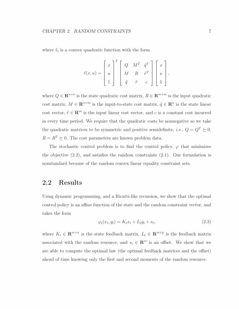
CHAPTER 2. RANDOM CONSTRAINTS 7
where ℓt is a convex quadratic function with the form
ℓ(x, u) =
x
u
1
T
Q MT qT
M R rT
q r c
x
u
1
,
where Q ∈ Rn×n is the state quadratic cost matrix, R ∈ Rm×m is the input quadratic
cost matrix, M ∈ Rn×m is the input-to-state cost matrix, q ∈ Rn is the state linear
cost vector, r ∈ Rm is the input linear cost vector, and c is a constant cost incurred
in every time period. We require that the quadratic costs be nonnegative so we take
the quadratic matrices to be symmetric and positive semidefinite, i.e., Q = QT � 0,
R = RT � 0. The cost parameters are known problem data.
The stochastic control problem is to find the control policy, ϕ that minimizes
the objective (2.2), and satisfies the random constraints (2.1). Our formulation is
nonstandard because of the random convex linear equality constraint sets.
2.2 Results
Using dynamic programming, and a Ricatti-like recursion, we show that the optimal
control policy is an affine function of the state and the random constraint vector, and
takes the form
ϕt(xt, gt) = Ktxt + Ltgt + st, (2.3)
where Kt ∈ Rm×n is the state feedback matrix, Lt ∈ Rm×p is the feedback matrix
associated with the random resource, and st ∈ Rm is an offset. We show that we
are able to compute the optimal law (the optimal feedback matrices and the offset)
ahead of time knowing only the first and second moments of the random resource.
CHAPTER 2. RANDOM CONSTRAINTS 8
2.3 Optimal policy via dynamic programming
We let Vt(z) denote the optimal objective value (minimum possible value of J) of the
truncated problem started in state xt = z at time period t. We will show that Vt(z)
is a convex quadratic function with the form
Vt(z) = (1/2)zTPtz + qTt z + rt, (2.4)
where Pt, qt, and rt are found by backward recursion. During our evaluation for Vt(z),
we will find an explicit expression for the optimal control policy which appears as an
intermediate result.
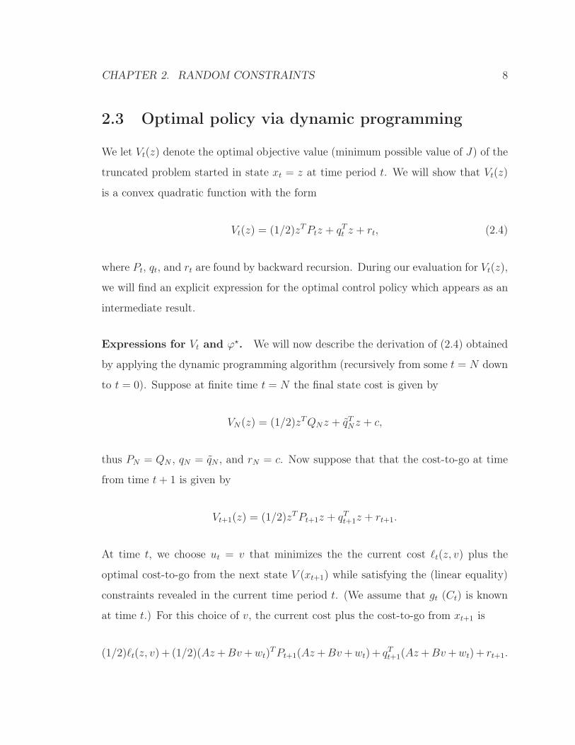
Expressions for Vt and ϕ⋆. We will now describe the derivation of (2.4) obtained
by applying the dynamic programming algorithm (recursively from some t = N down
to t = 0). Suppose at finite time t = N the final state cost is given by
VN(z) = (1/2)zTQNz + qTNz + c,
thus PN = QN , qN = qN , and rN = c. Now suppose that that the cost-to-go at time
from time t+ 1 is given by
Vt+1(z) = (1/2)zTPt+1z + qTt+1z + rt+1.
At time t, we choose ut = v that minimizes the the current cost ℓt(z, v) plus the
optimal cost-to-go from the next state V (xt+1) while satisfying the (linear equality)
constraints revealed in the current time period t. (We assume that gt (Ct) is known
at time t.) For this choice of v, the current cost plus the cost-to-go from xt+1 is
(1/2)ℓt(z, v) + (1/2)(Az+Bv+wt)TPt+1(Az+Bv+wt) + qTt+1(Az+Bv+wt) + rt+1.
CHAPTER 2. RANDOM CONSTRAINTS 9
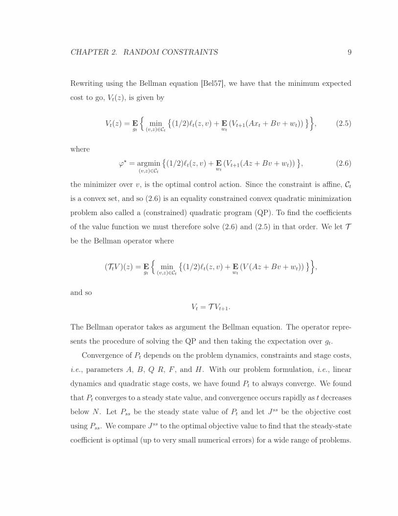
Rewriting using the Bellman equation [Bel57], we have that the minimum expected
cost to go, Vt(z), is given by
Vt(z) = Egt
{
min(v,z)∈Ct
{
(1/2)ℓt(z, v) + Ewt
(Vt+1(Axt +Bv + wt))}
}
, (2.5)
where
ϕ⋆ = argmin(v,z)∈Ct
{
(1/2)ℓt(z, v) + Ewt
(Vt+1(Az +Bv + wt))}
, (2.6)
the minimizer over v, is the optimal control action. Since the constraint is affine, Ct
is a convex set, and so (2.6) is an equality constrained convex quadratic minimization
problem also called a (constrained) quadratic program (QP). To find the coefficients
of the value function we must therefore solve (2.6) and (2.5) in that order. We let T
be the Bellman operator where
(TtV )(z) = Egt
{
min(v,z)∈Ct
{
(1/2)ℓt(z, v) + Ewt
(V (Az +Bv + wt))}
}
,
and so
Vt = T Vt+1.
The Bellman operator takes as argument the Bellman equation. The operator repre-
sents the procedure of solving the QP and then taking the expectation over gt.
Convergence of Pt depends on the problem dynamics, constraints and stage costs,
i.e., parameters A, B, Q R, F , and H . With our problem formulation, i.e., linear
dynamics and quadratic stage costs, we have found Pt to always converge. We found
that Pt converges to a steady state value, and convergence occurs rapidly as t decreases
below N . Let Pss be the steady state value of Pt and let Jss be the objective cost
using Pss. We compare Jss to the optimal objective value to find that the steady-state
coefficient is optimal (up to very small numerical errors) for a wide range of problems.
CHAPTER 2. RANDOM CONSTRAINTS 10
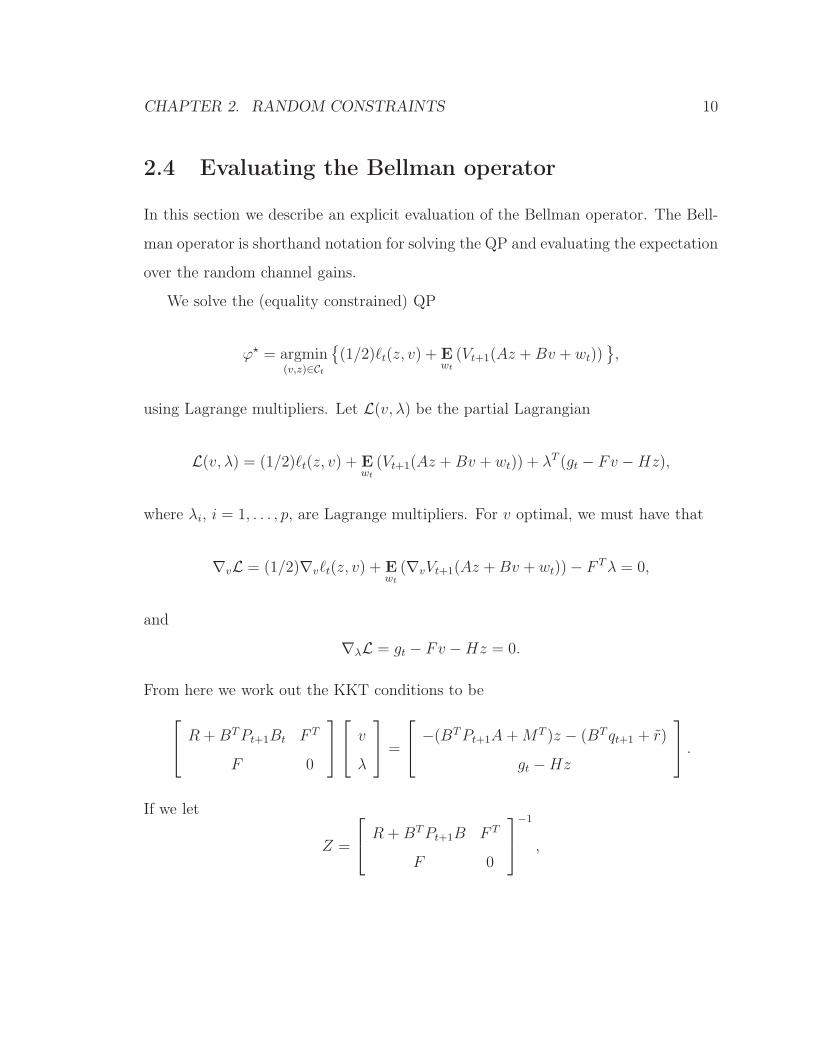
2.4 Evaluating the Bellman operator
In this section we describe an explicit evaluation of the Bellman operator. The Bell-
man operator is shorthand notation for solving the QP and evaluating the expectation
over the random channel gains.
We solve the (equality constrained) QP
ϕ⋆ = argmin(v,z)∈Ct
{
(1/2)ℓt(z, v) + Ewt
(Vt+1(Az +Bv + wt))}
,
using Lagrange multipliers. Let L(v, λ) be the partial Lagrangian
L(v, λ) = (1/2)ℓt(z, v) + Ewt
(Vt+1(Az +Bv + wt)) + λT (gt − Fv −Hz),
where λi, i = 1, . . . , p, are Lagrange multipliers. For v optimal, we must have that
∇vL = (1/2)∇vℓt(z, v) + Ewt
(∇vVt+1(Az +Bv + wt))− F Tλ = 0,
and
∇λL = gt − Fv −Hz = 0.
From here we work out the KKT conditions to be
R +BTPt+1Bt F T
F 0
v
λ
=
−(BTPt+1A +MT )z − (BT qt+1 + r)
gt −Hz
.
If we let
Z =
R + BTPt+1B F T
F 0
−1
,
CHAPTER 2. RANDOM CONSTRAINTS 11
we have that
v
λ
=
Z11 Z12
Z21 Z22
−(BTPt+1A+MT )z − (BT qt+1 + r)
gt −Hz
,
where Z11, Z12, Z21, Z22, are block matrix entries of Z. We can now write the
expression for the optimal input ϕ⋆ in terms of the entries of Z as
ϕ⋆ = v = −Z11(BTPt+1A+MT )z − Z12Hz + Z12gt − Z11(B
T qt+1 + r).
From (2.3) we get that our feedback matrices and offset as
Kt = −(Z11(BTPt+1A +MT ) + Z12H),
Lt = Z12,
st = −Z11(BT qt+1 + r).
The above are the components of the optimal control law. To evaluate the coeffi-
cients of our value function recursion, we must now substitute the optimal input ϕ⋆
into (2.5). We omit the cumbersome algebra and rewrite the resulting expression in
quadratic function form
T Vt+1 = Egt
1
2
z
gt
1
T
Y11 Y12 Y13
Y T12 Y22 Y23
Y T13 Y T
23 Y33
z
gt
1
,
CHAPTER 2. RANDOM CONSTRAINTS 12
where the symmetrized entries of Y are as follows
Y11 = Q+ 2MKt +KTt RKt + (A+BKt)
TPt+1(A +BKt),
Y12 = MLt +KTt RLt + (A +BKt)
TPt+1BLt,
Y13 = Mst +KTt Rst + (A +BKt)
T (Pt+1Bst + qt+1) +KTt r + q,
Y22 = LTt (R +BTPt+1B)Lt,
Y23 = LTt Rst + (BLt)
T (Pt+1Bst + qt+1) + LTt r,
Y33 = sTt (R +BTPt+1B)st + 2(rT + qTt+1B)st + 2rt+1 +Tr(WPt+1) + c.
Finally, the coefficients of (2.4) are given as
Pt = Y11, (2.7)
qt = Y12gt + Y13, (2.8)
rt =1
2Tr(GY22) + Y T
23gt +1
2Y33. (2.9)
Therefore for
Vt(z) = (1/2)zTPtz + qTt z + rt,
we get that
Pt = Q + 2MKt +KTt RKt + (A+BKt)
TPt+1(A+BKt),
qt = (MLt +KTt RLt + (A +BKt)
TPt+1BLt)gt
+ Mst +KTt Rst + (A+BKt)
T (Pt+1Bst + qt+1) +KT r + q,
rt = (1/2)Tr(GLTt (R +BTPt+1B)Lt) + LT
t Rst + (BLt)T (Pt+1Bst + qt+1) + LT r
+ (1/2)sTt (R +BTPt+1B)st + 2((rT + qTt+1B)st + ct + rt+1) +Tr(WPt+1),
CHAPTER 2. RANDOM CONSTRAINTS 13
where we substituted the optimal control ϕ⋆
ϕ⋆ = Ktz + Ltgt + st.
Note we should have that
FKt −H = 0, FLt = I, Fst = 0.
2.4.1 Remarks
In general there is no closed form analytical solution for a constrained QP. There
are, however, very efficient methods for solving QPs with convex equality constraints
including Lagrangian duality method that we employed above. For more on quadratic
optimization problems and efficient solution methods, see, e.g., [BL00, BNO03, BTN01,
Tuy98, BV04].
The analytic solution we obtain is inferred from our problem formulation. To see
this, note that the solution set of any consistent system of linear equations can be
written as an affine set [BV04, §2]. This is true for our problem since we have assumed
that the equality constraints are consistent, i.e., a feasible point (ut, xt) always exists.
Suppose we can parameterize explicitly the constraint set, C, using a free parameter
y ∈ Rk. We can write the set elements (fixed x) as
{(u, x) | (u = Gy + u, x)},
where u satisfies {u | F u + Hxt = gt}, and the columns of G ∈ Rm×k are in the
nullspace of F (N (F )). Analytically this says that the solution set is a hyperplane
and for our problem the parameters of the hyperplane consist of elements in the
random vector space.
CHAPTER 2. RANDOM CONSTRAINTS 14
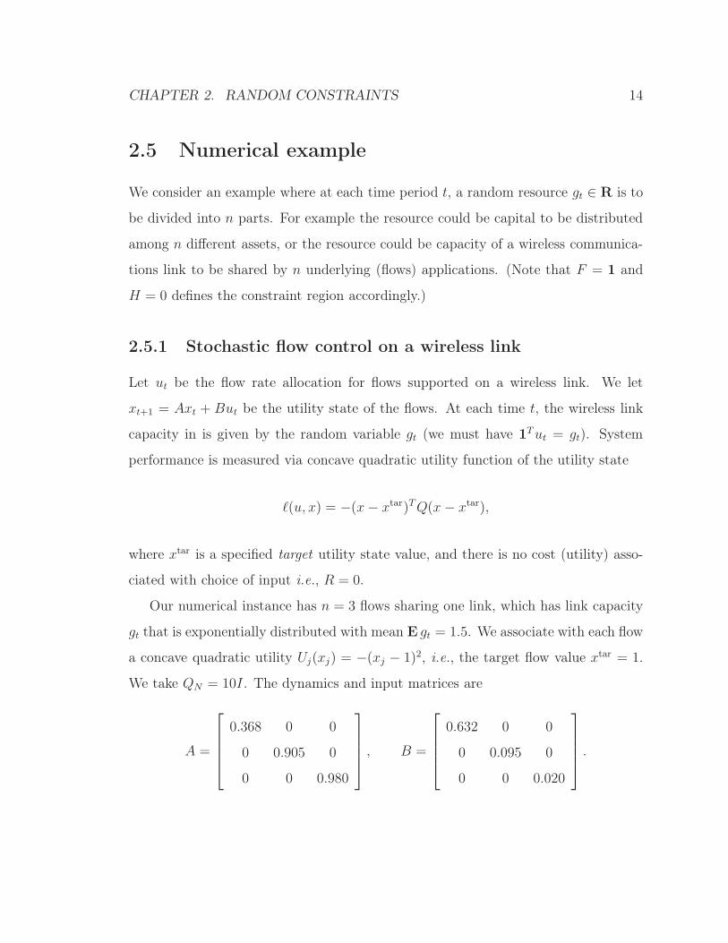
2.5 Numerical example
We consider an example where at each time period t, a random resource gt ∈ R is to
be divided into n parts. For example the resource could be capital to be distributed
among n different assets, or the resource could be capacity of a wireless communica-
tions link to be shared by n underlying (flows) applications. (Note that F = 1 and
H = 0 defines the constraint region accordingly.)
2.5.1 Stochastic flow control on a wireless link
Let ut be the flow rate allocation for flows supported on a wireless link. We let
xt+1 = Axt + But be the utility state of the flows. At each time t, the wireless link
capacity in is given by the random variable gt (we must have 1Tut = gt). System
performance is measured via concave quadratic utility function of the utility state
ℓ(u, x) = −(x− xtar)TQ(x− xtar),
where xtar is a specified target utility state value, and there is no cost (utility) asso-
ciated with choice of input i.e., R = 0.
Our numerical instance has n = 3 flows sharing one link, which has link capacity
gt that is exponentially distributed with mean E gt = 1.5. We associate with each flow
a concave quadratic utility Uj(xj) = −(xj − 1)2, i.e., the target flow value xtar = 1.
We take QN = 10I. The dynamics and input matrices are
A =
0.368 0 0
0 0.905 0
0 0 0.980
, B =
0.632 0 0
0 0.095 0
0 0 0.020
.
CHAPTER 2. RANDOM CONSTRAINTS 15
Results. We compute the optimal control law using the convex quadratic value
function (2.4), and the coefficients given in (2.7). The optimal control law is
ut =
−0.576 0.103 0.534
0.054 −8.627 4.586
0.522 8.525 −5.120
xt +
0.010
0.093
0.897
gt +
0.453
2.355
−2.808
.
We compare our policy to a simple equal sharing scheme: at each time period t, the
available (random) resource is divided equally among flows on the wireless link, i.e.,
ust =
1/3
1/3
1/3
gt.
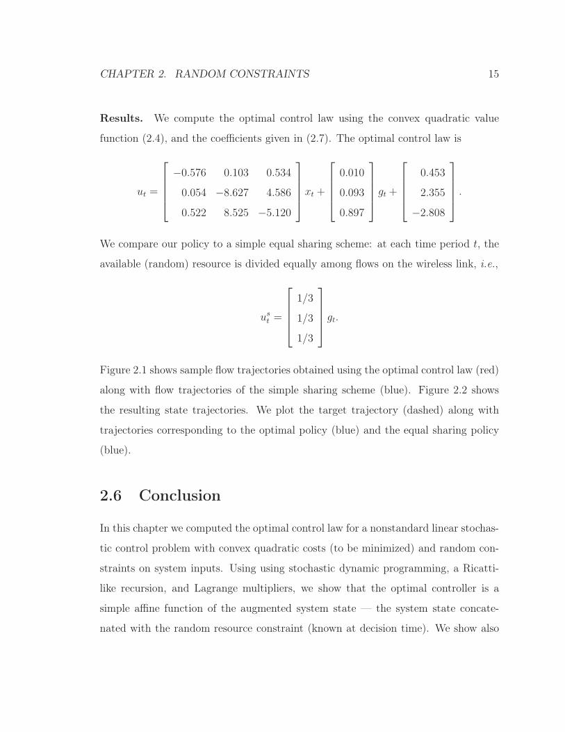
Figure 2.1 shows sample flow trajectories obtained using the optimal control law (red)
along with flow trajectories of the simple sharing scheme (blue). Figure 2.2 shows
the resulting state trajectories. We plot the target trajectory (dashed) along with
trajectories corresponding to the optimal policy (blue) and the equal sharing policy
(blue).
2.6 Conclusion
In this chapter we computed the optimal control law for a nonstandard linear stochas-
tic control problem with convex quadratic costs (to be minimized) and random con-
straints on system inputs. Using using stochastic dynamic programming, a Ricatti-
like recursion, and Lagrange multipliers, we show that the optimal controller is a
simple affine function of the augmented system state — the system state concate-
nated with the random resource constraint (known at decision time). We show also
CHAPTER 2. RANDOM CONSTRAINTS 16
flow
1flo
w2
flow
3
t10 20 30 40 50 60 70 80 90 100
10 20 30 40 50 60 70 80 90 100
10 20 30 40 50 60 70 80 90 100
0
2
4
6
0
2
4
6
0
2
4
6
Figure 2.1: Sample flow allocation trajectories, optimal policy (red), equal shar-ing policy (blue).

CHAPTER 2. RANDOM CONSTRAINTS 17
stat
e1
stat
e2
stat
e3
t10 20 30 40 50 60 70 80 90 100
10 20 30 40 50 60 70 80 90 100
10 20 30 40 50 60 70 80 90 100
0
1
2
0
1
2
0
1
2
Figure 2.2: Sample utility state trajectories, optimal policy (red), equal sharingpolicy (blue).
CHAPTER 2. RANDOM CONSTRAINTS 18
|xopt1 − xtar1 |
|xs1 − xtar1 |
0 0.1 0.2 0.3 0.4 0.5
0 0.1 0.2 0.3 0.4 0.5
0
10
20
30
40
0
10
20
30
40
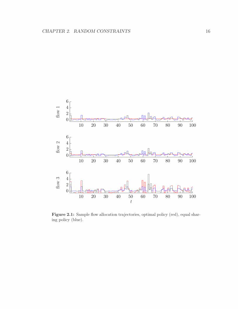
Figure 2.3: Error histograms for flow 1. Top. Absolute difference between theoptimal policy utility state and target utility state. Bottom. Absolute differencebetween the equal sharing utility state and target utility state.
CHAPTER 2. RANDOM CONSTRAINTS 19
|xopt2 − xtar2 |
|xs2 − xtar2 |
0 0.1 0.2 0.3 0.4 0.5
0 0.1 0.2 0.3 0.4 0.5
0
10
20
30
40
0
10
20
30
40
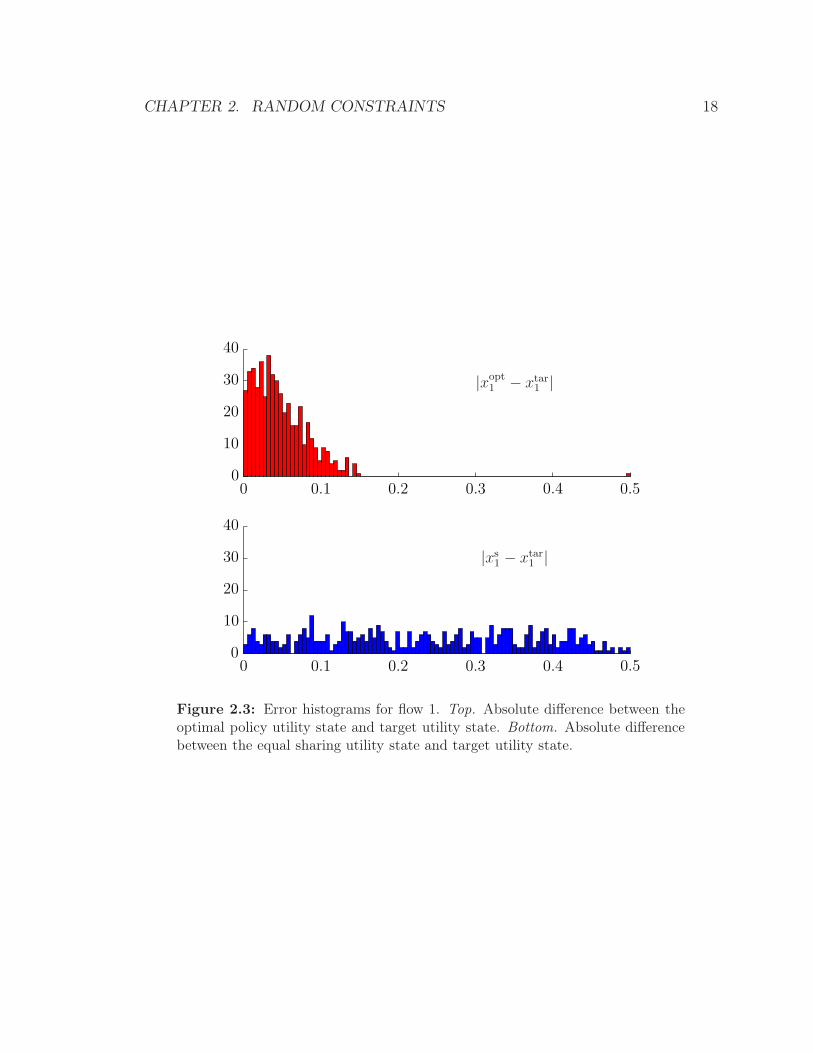
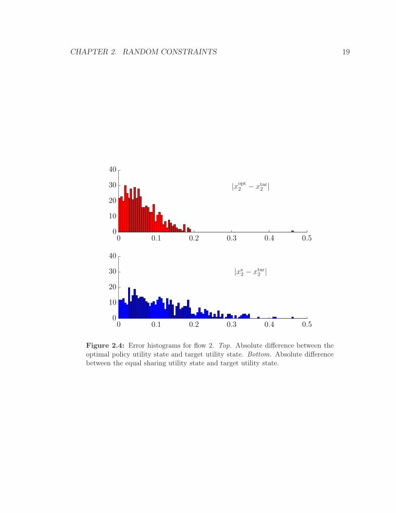
Figure 2.4: Error histograms for flow 2. Top. Absolute difference between theoptimal policy utility state and target utility state. Bottom. Absolute differencebetween the equal sharing utility state and target utility state.
CHAPTER 2. RANDOM CONSTRAINTS 20
|xopt3 − xtar3 |
|xs3 − xtar3 |
0 0.1 0.2 0.3 0.4 0.5
0 0.1 0.2 0.3 0.4 0.5
0
10
20
30
40
0
10
20
30
40
Figure 2.5: Error histograms for flow 3. Top. Absolute difference between theoptimal policy utility state and target utility state. Bottom. Absolute differencebetween the equal sharing utility state and target utility state.
CHAPTER 2. RANDOM CONSTRAINTS 21
that we can compute the optimal policy knowing only the first and second moments
of the random resource constraints.
We illustrate our optimal controller operation using a simple wireless link example
where flow rate (via random channel gain) is the random resource allocated. The
optimal controller gives significantly better results compared to an equal allocation
controller.
Chapter 3
Adaptive Modulation with Smoothed
Flow Utility
We consider the problem of choosing the data flow rate on a wireless link with ran-
domly varying channel gain, to optimally trade off average transmit power and the
average utility of the smoothed data flow rate. The smoothing allows us to model the
demands of an application that can tolerate variations in flow over a certain time in-
terval; we will see that this smoothing leads to a substantially different optimal data
flow rate policy than without smoothing. We pose the problem as a discrete-time
infinite-horizon stochastic control problem with linear dynamics, and convex objec-
tive. For the case of a single flow, the optimal data flow rate policy can be numerically
computed using stochastic dynamic programming and gridding. For the case of mul-
tiple flows on a single link, where dynamic programming becomes intractable due to
the curse of dimensionality, we propose an approximate dynamic programming ap-
proach to obtain suboptimal data flow rate policies. We illustrate, through numerical
examples, that these approximate policies can perform very well.
22

CHAPTER 3. SMOOTHING 23
3.1 Background
In the wireless communications literature, varying a link’s transmit rate (and power)
depending on channel conditions is called adaptive modulation; see, e.g., [Hay68,
Cav72, Hen74, WS95, GC97]. Adaptive modulation (and coding) schemes work with
the premise that channel state information is available at the transmitter, either via
feedback from the receiver, or using channel estimation techniques at the transmit-
ter. One drawback of adaptive modulation is that it is a physical layer optimization
technique with no knowledge of optimization protocols and techniques in the upper
layers.
Maximizing a total utility function is also very common in various communica-
tions and networking problem formulations, where it is referred to as network utility
maximization (NUM); see, e.g., [KMT97, LL99, CLCD07, NML08, CXH+10]. In the
NUM framework, performance of an upper layer protocol (e.g., TCP) is determined
by utility of flow attributes, e.g., utility of link flow rate.
Our setup involves both adaptive modulation and utility maximization, but is
nonstandard in several respects: We consider the utility of the smoothed flows, and
we consider multiple flows over the same wireless link [OABG10, AB10, ABO10].
3.2 Problem setup
channel RXTX
(Channel state information available)
CHAPTER 3. SMOOTHING 24
3.2.1 Average smoothed flow utility
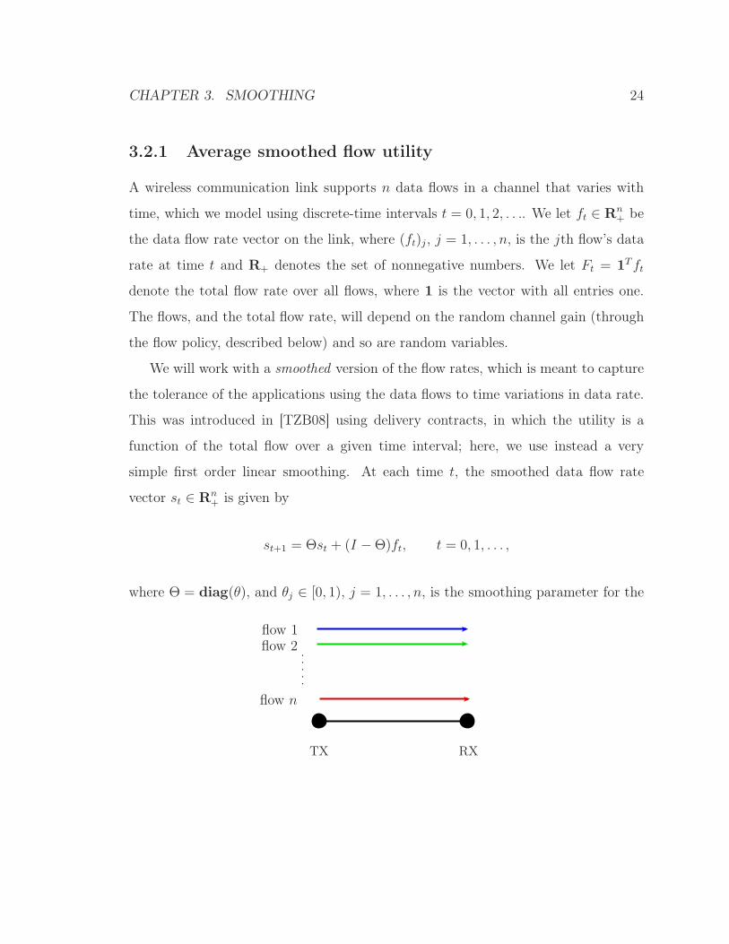
A wireless communication link supports n data flows in a channel that varies with
time, which we model using discrete-time intervals t = 0, 1, 2, . . .. We let ft ∈ Rn+ be
the data flow rate vector on the link, where (ft)j , j = 1, . . . , n, is the jth flow’s data
rate at time t and R+ denotes the set of nonnegative numbers. We let Ft = 1Tft
denote the total flow rate over all flows, where 1 is the vector with all entries one.
The flows, and the total flow rate, will depend on the random channel gain (through
the flow policy, described below) and so are random variables.
We will work with a smoothed version of the flow rates, which is meant to capture
the tolerance of the applications using the data flows to time variations in data rate.
This was introduced in [TZB08] using delivery contracts, in which the utility is a
function of the total flow over a given time interval; here, we use instead a very
simple first order linear smoothing. At each time t, the smoothed data flow rate
vector st ∈ Rn+ is given by
st+1 = Θst + (I −Θ)ft, t = 0, 1, . . . ,
where Θ = diag(θ), and θj ∈ [0, 1), j = 1, . . . , n, is the smoothing parameter for the
flow 1flow 2
flow n
TX RX
CHAPTER 3. SMOOTHING 25
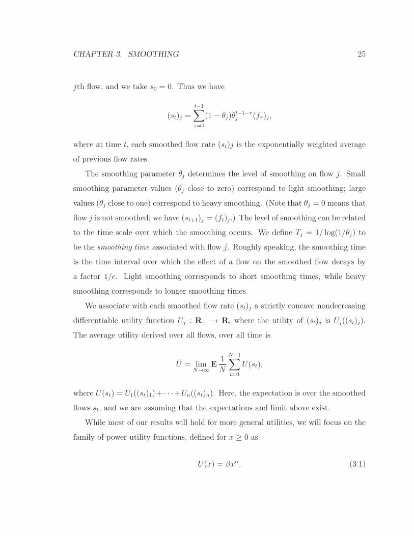
jth flow, and we take s0 = 0. Thus we have
(st)j =
t−1∑
τ=0
(1− θj)θt−1−τj (fτ )j ,
where at time t, each smoothed flow rate (st)j is the exponentially weighted average
of previous flow rates.
The smoothing parameter θj determines the level of smoothing on flow j. Small
smoothing parameter values (θj close to zero) correspond to light smoothing; large
values (θj close to one) correspond to heavy smoothing. (Note that θj = 0 means that
flow j is not smoothed; we have (st+1)j = (ft)j.) The level of smoothing can be related
to the time scale over which the smoothing occurs. We define Tj = 1/ log(1/θj) to
be the smoothing time associated with flow j. Roughly speaking, the smoothing time
is the time interval over which the effect of a flow on the smoothed flow decays by
a factor 1/e. Light smoothing corresponds to short smoothing times, while heavy
smoothing corresponds to longer smoothing times.
We associate with each smoothed flow rate (st)j a strictly concave nondecreasing
differentiable utility function Uj : R+ → R, where the utility of (st)j is Uj((st)j).
The average utility derived over all flows, over all time is
U = limN→∞
E1
N
N−1∑
t=0
U(st),
where U(st) = U1((st)1)+ · · ·+Un((st)n). Here, the expectation is over the smoothed
flows st, and we are assuming that the expectations and limit above exist.
While most of our results will hold for more general utilities, we will focus on the
family of power utility functions, defined for x ≥ 0 as
U(x) = βxα, (3.1)
CHAPTER 3. SMOOTHING 26
parameterized by α ∈ (0, 1) and β > 0. The parameter α sets the curvature (or risk
aversion), while β sets the overall weight of the utility. (For small values of α, U
approaches a log utility.)
Before proceeding, we make some general comments on our use of smoothed flows.
The smoothing can be considered a type of time averaging; then we apply a concave
utility function; and finally, we average this utility. The time averaging and utility
function operations do not commute, except in the case when the utility is linear (or
affine). Jensen’s inequality tells us that average smoothed utility is greater than or
equal to the average utility applied directly to the flow rates, i.e.,
U((st)j) ≥1
t
t−1∑
τ=0
(1− θj)θt−1−τj U(fτ )j .
So the time smoothing step does affect our average utility; we will see later that it
has a dramatic affect on the optimal flow policy.
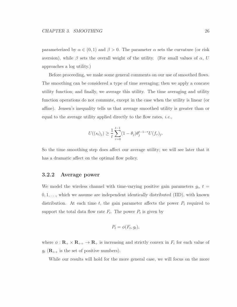
3.2.2 Average power
We model the wireless channel with time-varying positive gain parameters gt, t =
0, 1, . . ., which we assume are independent identically distributed (IID), with known
distribution. At each time t, the gain parameter affects the power Pt required to
support the total data flow rate Ft. The power Pt is given by
Pt = φ(Ft, gt),
where φ : R+ × R++ → R+ is increasing and strictly convex in Ft for each value of
gt (R++ is the set of positive numbers).
While our results will hold for the more general case, we will focus on the more
CHAPTER 3. SMOOTHING 27
specific power function described here. We suppose that the signal-to-interference-
and-noise (SINR) of the channel is given by gtPt. (Here gt includes the effect of
time-varying channel gain, noise, and interference.) The channel capacity is then
µ log(1 + gtPt), where µ is a constant; this must equal at least the total flow rate Ft,
so we obtain
Pt = φ(Ft, gt) =eFt/µ − 1
gt. (3.2)
The total average power is
P = limN→∞
E1
N
N−1∑
t=0
Pt,
where again, we are assuming that the expectations and limit exist.
3.2.3 Flow rate control problem
The overall objective is to maximize a weighted difference between average utility and
average power,
J = U − λP , (3.3)
where λ ∈ R++ is used to trade off average utility and power.
We require that the flow policy is causal, i.e., when ft is chosen, we know the
previous and current values of the flows, smoothed flows, and channel gains. Standard
arguments in stochastic control (see, e.g., [Ber05, Ber07, Åst70, Whi82, BS96]) can
be used to conclude that, without loss of generality, we can assume that the flow
control policy has the form
ft = ϕ(st, gt), (3.4)
where ϕ : Rn+ × R++ → Rn
+. In other words, the policy depends only on the current
smoothed flows, and the current channel gain value.
The flow rate control problem is to choose the flow rate policy ϕ to maximize the
CHAPTER 3. SMOOTHING 28
overall objective in (3.3). This is a standard convex stochastic control problem, with
linear dynamics.
3.2.4 Our results
We let J⋆ be the optimal overall objective value, and ϕ⋆ be an optimal policy. We
will show that in the general (multiple flow) case, the optimal policy includes a “no-
transmit" zone, i.e., a region in the (st, gt) space in which the optimal flow rate is
zero. Not surprisingly, the optimal flow policy can be roughly described as waiting
until the channel gain is large, or until the smoothed flow has fallen to a low level, at
which point we transmit (i.e., choose nonzero ft). Roughly speaking, the higher the
level of smoothing, the longer we can afford to wait for a large channel gain before
transmitting. The average power required to support a given utility level decreases,
sometimes dramatically, as the level of smoothing increases.
We show that the optimal policy for the case of a single flow is readily computed
numerically, working from Bellman’s [Bel57] characterization of the optimal policy,
and is not particularly sensitive to the details of the utility functions, smoothing
levels, or power functions.
For the case of multiple flows, we cannot easily compute (or even represent) the
optimal policy. For this case we propose an approximate policy, based on approximate
dynamic programming [BT96, Pow07]. By computing an upper bound on J⋆, by
allowing the flow control policy to use future values of channel gain (i.e., relaxing the
causality requirement [BSS10]), we show in numerical experiments that such policies
are nearly optimal.
CHAPTER 3. SMOOTHING 29
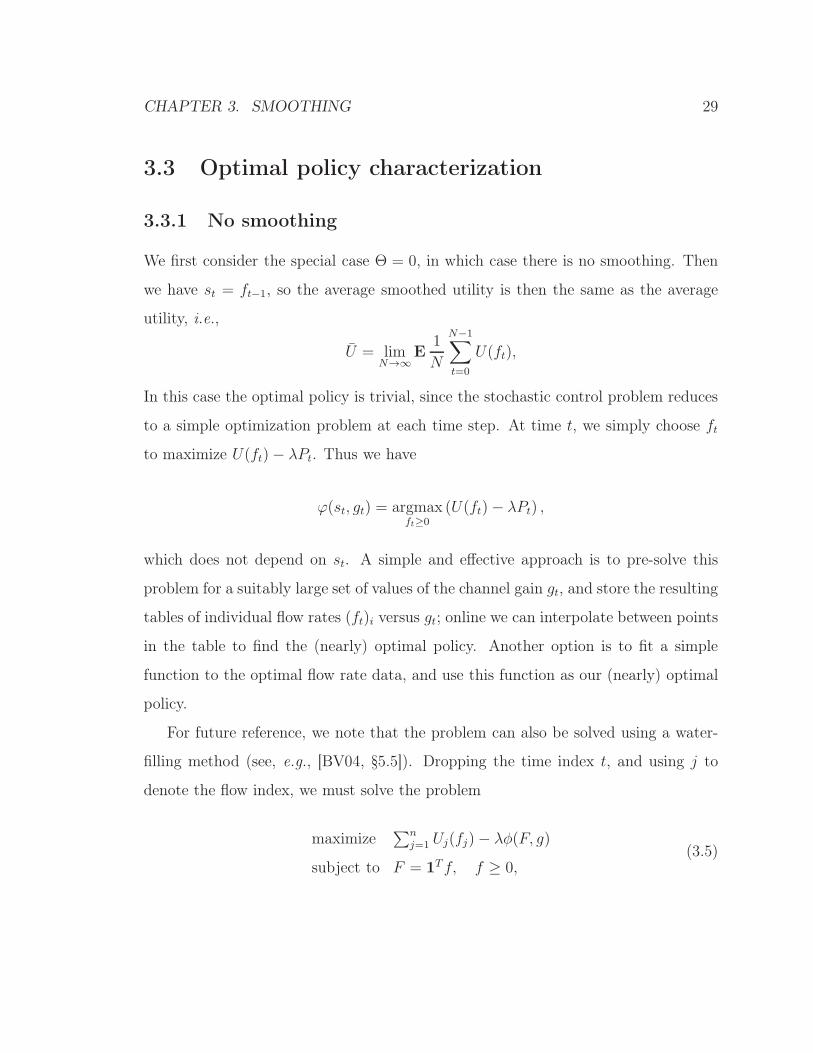
3.3 Optimal policy characterization
3.3.1 No smoothing
We first consider the special case Θ = 0, in which case there is no smoothing. Then
we have st = ft−1, so the average smoothed utility is then the same as the average
utility, i.e.,
U = limN→∞
E1
N
N−1∑
t=0
U(ft),
In this case the optimal policy is trivial, since the stochastic control problem reduces
to a simple optimization problem at each time step. At time t, we simply choose ft
to maximize U(ft)− λPt. Thus we have
ϕ(st, gt) = argmaxft≥0
(U(ft)− λPt) ,
which does not depend on st. A simple and effective approach is to pre-solve this
problem for a suitably large set of values of the channel gain gt, and store the resulting
tables of individual flow rates (ft)i versus gt; online we can interpolate between points
in the table to find the (nearly) optimal policy. Another option is to fit a simple
function to the optimal flow rate data, and use this function as our (nearly) optimal
policy.
For future reference, we note that the problem can also be solved using a water-
filling method (see, e.g., [BV04, §5.5]). Dropping the time index t, and using j to
denote the flow index, we must solve the problem
maximize∑n
j=1 Uj(fj)− λφ(F, g)
subject to F = 1Tf, f ≥ 0,(3.5)
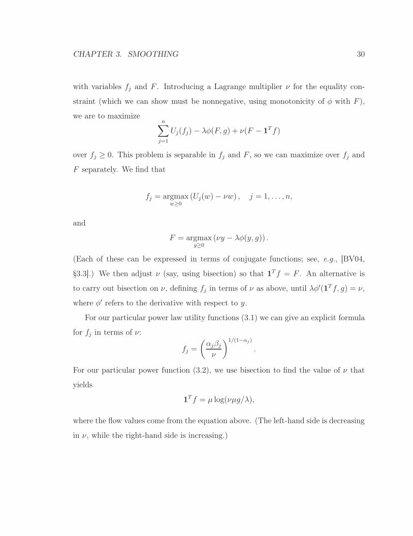
CHAPTER 3. SMOOTHING 30
with variables fj and F . Introducing a Lagrange multiplier ν for the equality con-
straint (which we can show must be nonnegative, using monotonicity of φ with F ),
we are to maximizen∑
j=1
Uj(fj)− λφ(F, g) + ν(F − 1Tf)
over fj ≥ 0. This problem is separable in fj and F , so we can maximize over fj and
F separately. We find that
fj = argmaxw≥0
(Uj(w)− νw) , j = 1, . . . , n,
and
F = argmaxy≥0
(νy − λφ(y, g)) .
(Each of these can be expressed in terms of conjugate functions; see, e.g., [BV04,
§3.3].) We then adjust ν (say, using bisection) so that 1Tf = F . An alternative is
to carry out bisection on ν, defining fj in terms of ν as above, until λφ′(1Tf, g) = ν,
where φ′ refers to the derivative with respect to y.
For our particular power law utility functions (3.1) we can give an explicit formula
for fj in terms of ν:
fj =
(
αjβjν
)1/(1−αj )
.
For our particular power function (3.2), we use bisection to find the value of ν that
yields
1T f = µ log(νµg/λ),
where the flow values come from the equation above. (The left-hand side is decreasing
in ν, while the right-hand side is increasing.)

CHAPTER 3. SMOOTHING 31
3.3.2 General case
We now consider the more general case, with smoothing. We can characterize the
optimal flow rate policy ϕ⋆ using stochastic dynamic programming [Put94, Ros83a,
Den82, WB09] and a form of Bellman’s equation [Bel57]. The optimal flow rate policy
has the form
ϕ⋆(z, g) = argmaxw≥0
(
V (Θz + (I −Θ)w)− λφ(1Tw, g))
, (3.6)
where V : Rn+ → R is the Bellman (relative) value function. The value function (and
optimal value) is characterized via the fixed point equation
J⋆ + V = T V, (3.7)
where for any function W : Rn+ → R, the Bellman operator T is given by
(TW )(z) = U(z) + E
(
maxw≥0
(
W (Θz + (I −Θ)w)− λφ(1Tw, g))
)
,
where the expectation is over g. The fixed point equation and Bellman operator are
invariant under adding a constant; that is, we have T (W + a) = TW + a, for any
constant (function) a, and similarly, V satisfies the fixed point equation if and only
if V + a does. So without loss of generality we can assume that V (0) = 0.
3.3.3 Value iteration
In this section we describe the numerical value iteration algorithm we use for our
average (cost) utility problem. For more technical details on value iteration (and
policy iteration) we refer the reader to [Bla62, Der66, Der70, ABFG+93, Sen96, Ber98,
Ber05, Ber07].
CHAPTER 3. SMOOTHING 32
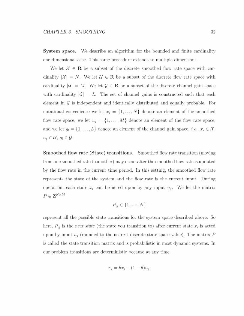
System space. We describe an algorithm for the bounded and finite cardinality
one dimensional case. This same procedure extends to multiple dimensions.
We let X ∈ R be a subset of the discrete smoothed flow rate space with car-
dinality |X | = N . We let U ∈ R be a subset of the discrete flow rate space with
cardinality |U| = M . We let G ∈ R be a subset of the discrete channel gain space
with cardinality |G| = L. The set of channel gains is constructed such that each
element in G is independent and identically distributed and equally probable. For
notational convenience we let xi = {1, . . . , N} denote an element of the smoothed
flow rate space, we let uj = {1, . . . ,M} denote an element of the flow rate space,
and we let gl = {1, . . . , L} denote an element of the channel gain space, i.e., xi ∈ X ,
uj ∈ U , gl ∈ G.
Smoothed flow rate (State) transitions. Smoothed flow rate transition (moving
from one smoothed rate to another) may occur after the smoothed flow rate is updated
by the flow rate in the current time period. In this setting, the smoothed flow rate
represents the state of the system and the flow rate is the current input. During
operation, each state xi can be acted upon by any input uj. We let the matrix
P ∈ ZN×M
Pij ∈ {1, . . . , N}
represent all the possible state transitions for the system space described above. So
here, Pij is the next state (the state you transition to) after current state xi is acted
upon by input uj (rounded to the nearest discrete state space value). The matrix P
is called the state transition matrix and is probabilistic in most dynamic systems. In
our problem transitions are deterministic because at any time
xk = θxi + (1− θ)uj,
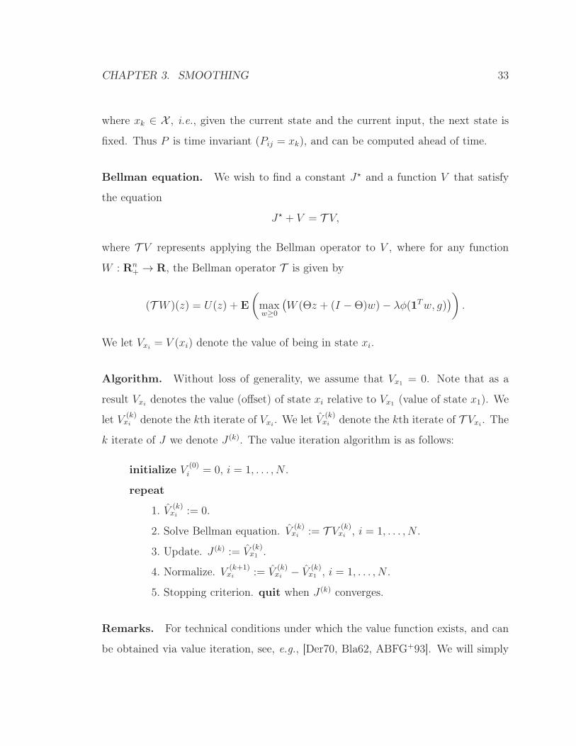
CHAPTER 3. SMOOTHING 33
where xk ∈ X , i.e., given the current state and the current input, the next state is
fixed. Thus P is time invariant (Pij = xk), and can be computed ahead of time.
Bellman equation. We wish to find a constant J⋆ and a function V that satisfy
the equation
J⋆ + V = T V,
where T V represents applying the Bellman operator to V , where for any function
W : Rn+ → R, the Bellman operator T is given by
(TW )(z) = U(z) + E
(
maxw≥0
(
W (Θz + (I −Θ)w)− λφ(1Tw, g))
)
.
We let Vxi= V (xi) denote the value of being in state xi.
Algorithm. Without loss of generality, we assume that Vx1 = 0. Note that as a
result Vxidenotes the value (offset) of state xi relative to Vx1 (value of state x1). We
let V (k)xi denote the kth iterate of Vxi
. We let V (k)xi denote the kth iterate of T Vxi
. The
k iterate of J we denote J (k). The value iteration algorithm is as follows:
initialize V(0)i = 0, i = 1, . . . , N .
repeat
1. V (k)xi := 0.
2. Solve Bellman equation. V (k)xi := T V (k)
xi , i = 1, . . . , N .
3. Update. J (k) := V(k)x1 .
4. Normalize. V (k+1)xi := V
(k)xi − V
(k)x1 , i = 1, . . . , N .
5. Stopping criterion. quit when J (k) converges.
Remarks. For technical conditions under which the value function exists, and can
be obtained via value iteration, see, e.g., [Der70, Bla62, ABFG+93]. We will simply
CHAPTER 3. SMOOTHING 34
assume here that the value function exists, and J (k) and V (k) converge to J⋆ and V ,
respectively. (The algorithm converged for all the simulations we performed using
several different values for the smoothing parameter and multiple utility function
parameters.)
The iterations above preserve several attributes of the iterates, which we can then
conclude holds for V . First of all, concavity of V (k) is preserved, i.e., if V (k) is concave,
so is V (k+1). It is clear that normalization does not affect concavity, since we simply
add a constant to the function. The Bellman operator T preserves concavity since
partial maximization of a function concave in two sets of variables results in a concave
function (see, i.e., [BV04, §3.2]), and expectation over a family of concave functions
yields a concave function; finally, addition (of U) preserves concavity. So we can
conclude that V is concave.
Another attribute that is preserved in value iteration is monotonicity; if V (k) is
monotone increasing (in each component of its argument), then so is V (k+1). We
conclude that V is monotone increasing.
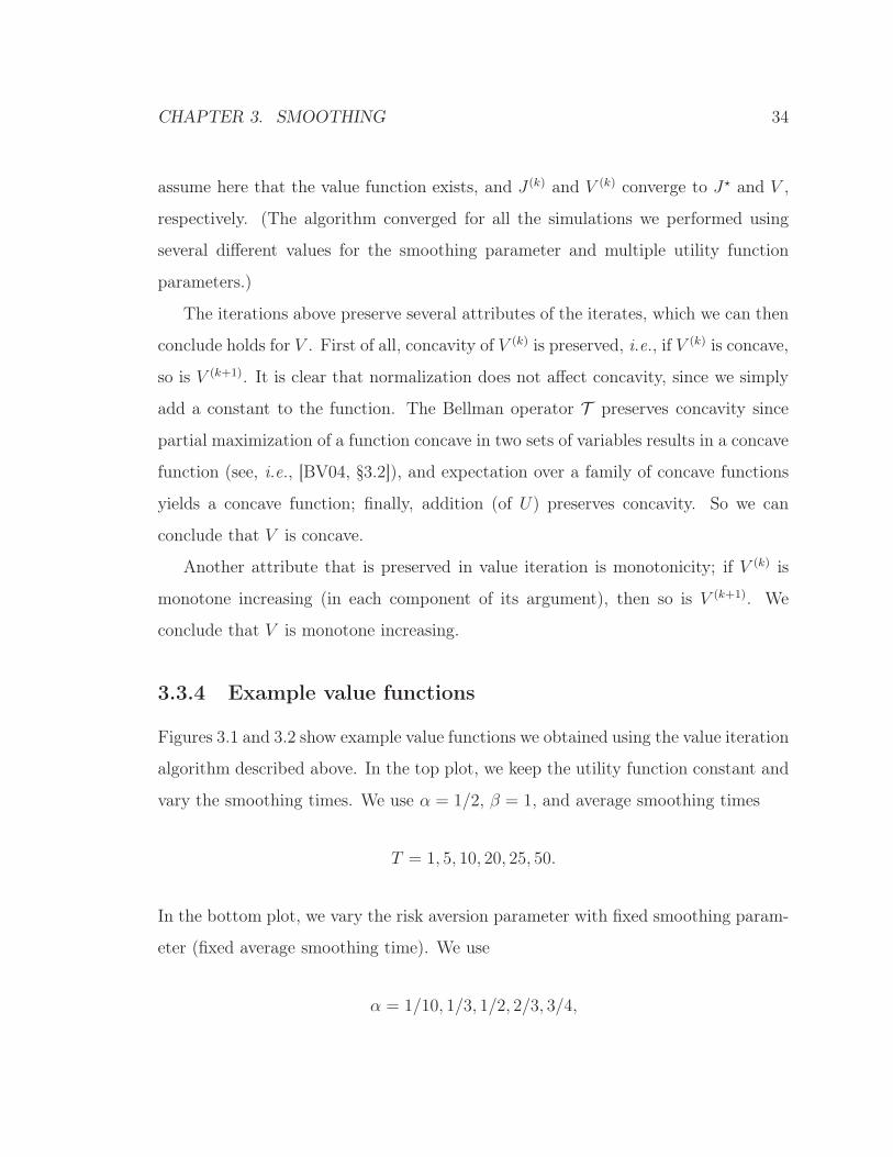
3.3.4 Example value functions
Figures 3.1 and 3.2 show example value functions we obtained using the value iteration
algorithm described above. In the top plot, we keep the utility function constant and
vary the smoothing times. We use α = 1/2, β = 1, and average smoothing times
T = 1, 5, 10, 20, 25, 50.
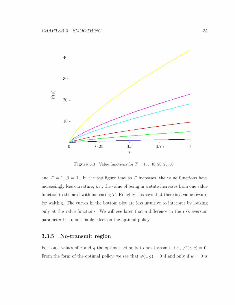
In the bottom plot, we vary the risk aversion parameter with fixed smoothing param-
eter (fixed average smoothing time). We use
α = 1/10, 1/3, 1/2, 2/3, 3/4,
CHAPTER 3. SMOOTHING 35
s
V(s)
0 0.25 0.5 0.75 1
10
20
30
40
Figure 3.1: Value functions for T = 1, 5, 10, 20, 25, 50.
and T = 1, β = 1. In the top figure that as T increases, the value functions have
increasingly less curvature, i.e., the value of being in a state increases from one value
function to the next with increasing T . Roughly this says that there is a value reward
for waiting. The curves in the bottom plot are less intuitive to interpret by looking
only at the value functions. We will see later that a difference in the risk aversion
parameter has quantifiable effect on the optimal policy.
3.3.5 No-transmit region
For some values of z and g the optimal action is to not transmit, i.e., ϕ⋆(z, g) = 0.
From the form of the optimal policy, we see that ϕ(z, g) = 0 if and only if w = 0 is
CHAPTER 3. SMOOTHING 36
s
V(s)
0 0.25 0.5 0.75 1
0.5
1
1.5
Figure 3.2: Value functions for α = 1/10, 1/3, 1/2, 2/3, 3/4.
CHAPTER 3. SMOOTHING 37
optimal for the (convex) problem
maximize V (Θz + (I −Θ)w)− λφ(1Tw, g)
subject to w ≥ 0,
with variable w ∈ Rn. This is the case if and only if
−λ∇φ(0, g) ∈ ∂(−V (Θz)),
where ∂ denotes the subdifferential.
Differentiable V . For V differentiable, the optimality conditions simplify to give
(I −Θ)∇V (Θz) + λφ′(0, g)1 ≤ 0
(see, e.g., [BV04, p142]). We can rewrite this as
∂V
∂zi(Θz) ≤
λφ′(0, g)
1− θi, i = 1, . . . , n.
Using the specific power function (3.2) associated with the log capacity formula, we
obtain
∇V (Θz) ≤λ
µg
(
1
1− θ1, . . . ,
1
1− θn
)
(3.8)
as the necessary and sufficient condition under which ϕ(z, g) = 0. Since ∇V is
decreasing (by concavity of V ), we can interpret (3.8) roughly as follows: Do not
transmit if the channel is bad (g small) or if the smoothed flows are large (z large).
CHAPTER 3. SMOOTHING 38
3.4 Single flow case
3.4.1 Optimal policy
In the case of a single flow (i.e., n = 1) we can easily carry out value iteration numer-
ically, by discretizing the argument z and values of g, and computing the expectation
and maximization numerically. For the single flow case, then, we can compute the
optimal policy and optimal performance (up to small numerical integration errors).
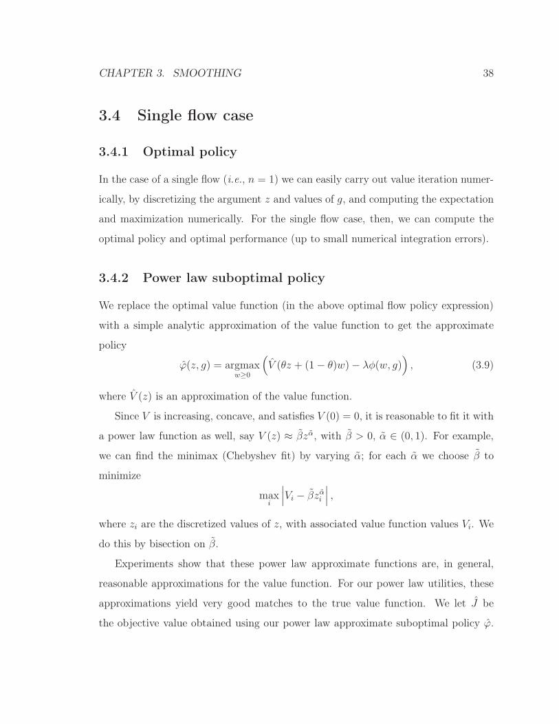
3.4.2 Power law suboptimal policy
We replace the optimal value function (in the above optimal flow policy expression)
with a simple analytic approximation of the value function to get the approximate
policy
ϕ(z, g) = argmaxw≥0
(
V (θz + (1− θ)w)− λφ(w, g))
, (3.9)
where V (z) is an approximation of the value function.
Since V is increasing, concave, and satisfies V (0) = 0, it is reasonable to fit it with
a power law function as well, say V (z) ≈ βzα, with β > 0, α ∈ (0, 1). For example,
we can find the minimax (Chebyshev fit) by varying α; for each α we choose β to
minimize
maxi
∣
∣
∣Vi − βzαi
∣
∣
∣,
where zi are the discretized values of z, with associated value function values Vi. We
do this by bisection on β.
Experiments show that these power law approximate functions are, in general,
reasonable approximations for the value function. For our power law utilities, these
approximations yield very good matches to the true value function. We let J be
the objective value obtained using our power law approximate suboptimal policy ϕ.
CHAPTER 3. SMOOTHING 39
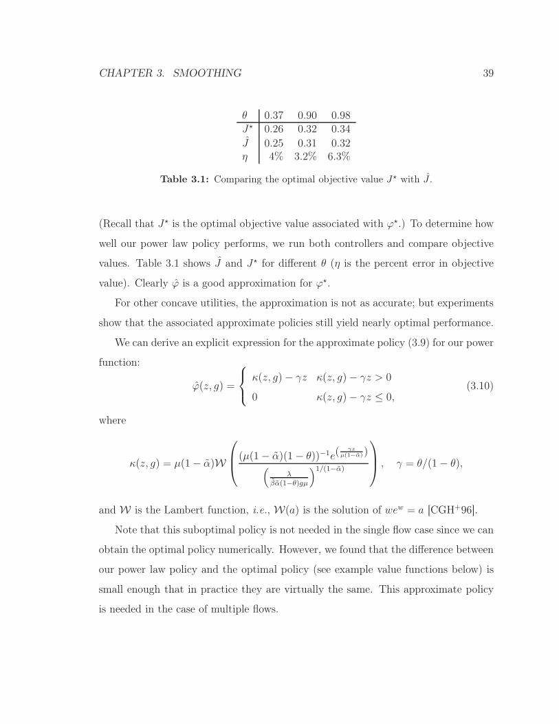
θ 0.37 0.90 0.98J⋆ 0.26 0.32 0.34J 0.25 0.31 0.32η 4% 3.2% 6.3%
Table 3.1: Comparing the optimal objective value J⋆ with J .
(Recall that J⋆ is the optimal objective value associated with ϕ⋆.) To determine how
well our power law policy performs, we run both controllers and compare objective
values. Table 3.1 shows J and J⋆ for different θ (η is the percent error in objective
value). Clearly ϕ is a good approximation for ϕ⋆.
For other concave utilities, the approximation is not as accurate; but experiments
show that the associated approximate policies still yield nearly optimal performance.
We can derive an explicit expression for the approximate policy (3.9) for our power
function:
ϕ(z, g) =
κ(z, g)− γz κ(z, g)− γz > 0
0 κ(z, g)− γz ≤ 0,(3.10)
where
κ(z, g) = µ(1− α)W
(µ(1− α)(1− θ))−1e(γz
µ(1−α))
(
λβα(1−θ)gµ
)1/(1−α)
, γ = θ/(1− θ),
and W is the Lambert function, i.e., W(a) is the solution of wew = a [CGH+96].
Note that this suboptimal policy is not needed in the single flow case since we can
obtain the optimal policy numerically. However, we found that the difference between
our power law policy and the optimal policy (see example value functions below) is
small enough that in practice they are virtually the same. This approximate policy
is needed in the case of multiple flows.
CHAPTER 3. SMOOTHING 40
3.4.3 Example
In this section we give simple numerical examples to illustrate the effect of smoothing
on the resulting flow rate policy in the single flow case. We consider two examples,
with different levels of smoothing. The first flow is lightly smoothed (T = 1; θ = 0.37),
while the second flow is heavily smoothed (T = 50; θ = 0.98). We use utility function
U(s) = s1/2, i.e., α = 1/2, β = 1 in our utility (3.1). The channel gains gt are IID
exponential variables with mean E gt = 1. We use the power function (3.2), with
µ = 1.
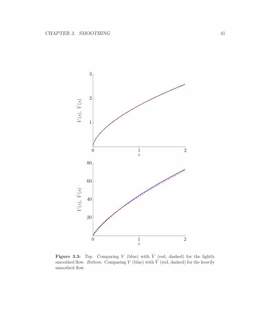
We first consider the case λ = 1. The value functions are shown in figure 3.3,
together with the power law approximations, which are 1.7s0.6 (light smoothing) and
42.7s0.74 (heavy smoothing). Figure 3.4 shows the optimal policies for the lightly
smoothed flow (θ = 0.37), and the heavily smoothed flow (θ = 0.98). We can see
that the optimal policies are quite different. As expected, the lightly smoothed flow
transmits more often, i.e., has a smaller no-transmit region.
Average power vs average utility. Figure 3.5 further illustrates the difference
between the two flow rate policies. Using values of λ ∈ (0, 1], we computed (via sim-
ulation) the average power-average utility trade-off curve for each flow. As expected,
we can see that the heavily smoothed flow achieves more average utility, for a given
average power, than the lightly smoothed flow. (The heavily smoothed flow requires
less average power to achieve a target average utility.)
Comparing average power. We compare the average power required by each flow
to generate a given average utility. Given a target average utility, we can estimate
the average power required roughly from figure 3.5, or more precisely via simulation
as follows: choose a target average utility, and then run each controller, adjusting
λ separately, until we reach the target utility. In our example, we chose U = 0.7
CHAPTER 3. SMOOTHING 41
s
V(s),V(s)
0 1 2
1
2
3
s
V(s),V(s)
0 1 2
20
40
60
80
Figure 3.3: Top. Comparing V (blue) with V (red, dashed) for the lightlysmoothed flow. Bottom. Comparing V (blue) with V (red, dashed) for the heavilysmoothed flow.
CHAPTER 3. SMOOTHING 42
01
23
45
0
1
2
3
0
0.5
1
1.5
g
ϕ⋆(s,g)
01
23
45
0
1
2
3
0
0.5
1
1.5
gs
ϕ⋆(s,g)
Figure 3.4: Top. Optimal policy ϕ⋆(s, g) for smoothing time T = 1 (θ = 0.37).Bottom. Optimal policy for T = 50 (θ = 0.98).
CHAPTER 3. SMOOTHING 43
0 0.5 1 1.5 2 2.5 3
0.4
0.5
0.6
0.7
0.8
0.9
1
P
U
Figure 3.5: Average utility versus average power; heavily smoothed flow (top,dashed), lightly smoothed flow (bottom).
and found λ = 0.29 for the lightly smoothed flow, and λ = 0.35 for the heavily
smoothed flow. Figure 3.6 shows the associated power trajectories for each flow, along
with the corresponding flow and smoothed flow trajectories. The dashed (horizontal)
line indicates the average power, average flow, and averaged smoothed flow for each
trajectory. Clearly the lightly smoothed flow requires more power than the heavily
smoothed flow, by around 25%: the heavily smoothed flow requires P = 0.7, compared
to P = 0.93 for the lightly smoothed flow.
CHAPTER 3. SMOOTHING 44
0 50 1000
0.5
1
1.5
0 50 1000
0.5
1
1.5
0 50 1000
0.51
1.52
0 50 1000
0.51
1.52
0 50 1000
0.5
1
1.5
0 50 1000
0.5
1
1.5
P
tt
sf
Figure 3.6: Sample power, flow, and smoothed flow trajectories; lightlysmoothed flow (left), heavily smoothed flow (right).
CHAPTER 3. SMOOTHING 45
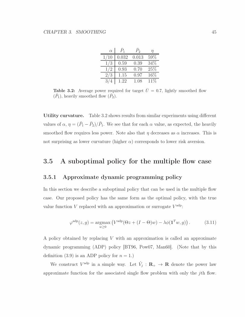
α P1 P2 η
1/10 0.032 0.013 59%1/3 0.59 0.39 34%1/2 0.93 0.70 25%2/3 1.15 0.97 16%3/4 1.22 1.08 11%
Table 3.2: Average power required for target U = 0.7, lightly smoothed flow(P1), heavily smoothed flow (P2).
Utility curvature. Table 3.2 shows results from similar experiments using different
values of α, η = (P1 − P2)/P1. We see that for each α value, as expected, the heavily
smoothed flow requires less power. Note also that η decreases as α increases. This is
not surprising as lower curvature (higher α) corresponds to lower risk aversion.
3.5 A suboptimal policy for the multiple flow case
3.5.1 Approximate dynamic programming policy
In this section we describe a suboptimal policy that can be used in the multiple flow
case. Our proposed policy has the same form as the optimal policy, with the true
value function V replaced with an approximation or surrogate V adp:
ϕadp(z, g) = argmaxw≥0
(
V adp(Θz + (I −Θ)w)− λφ(1Tw, g))
. (3.11)
A policy obtained by replacing V with an approximation is called an approximate
dynamic programming (ADP) policy [BT96, Pow07, Man60]. (Note that by this
definition (3.9) is an ADP policy for n = 1.)
We construct V adp in a simple way. Let Vj : R+ → R denote the power law
approximate function for the associated single flow problem with only the jth flow.
CHAPTER 3. SMOOTHING 46
(This can obtained numerically as described above.) We then take
V adp(z) = V1(z1) + · · ·+ Vn(zn).
This approximate value function is separable, i.e., a sum of functions of the indi-
vidual flows, whereas the exact value function is (in general) not. The approximate
policy, however, is not separable; the optimization problem solving to assign flow
rates couples the different flow rates.
In the literature on approximate dynamic programming, Vj would be considered
basis functions [SS85, TZ97, dFR03]; however, we fix the coefficients of the basis
functions as one. (We have found that very little improvement in the policy is obtained
by optimizing over the coefficients.) Evaluating the approximate policy, i.e., solving
(3.11), reduces to solving the optimization problem
maximize∑n
j=1 Vj(θjzj − (1− θj)fj)− λφ(F, g)
subject to F = 1Tf, fj ≥ 0, j = 1, . . . , n,(3.12)
with optimization variables fj, F . This is a convex optimization problem; its special
structure allows it to be solved extremely efficiently, via water-filling. We let
Jadp = Uadp − λP adp,
denote the objective value obtained using our ADP policy.
3.5.2 Solution via water-filling
In this section we give a solution (3.12) using the water-filling method described earlier
in §3.3.1. Recall the single flow power law approximate functions Vj(zj) = βjzαj .
CHAPTER 3. SMOOTHING 47
Substituting into our expression for V adp we get
V adp(z) =n∑
j=1
βjzαj .
The resulting resource allocation problem is
maximize∑n
j=1 βj(θjzj − (1− θj)fj)αj − λφ(F, g)
subject to F = 1Tf, fj ≥ 0, j = 1, . . . , n,
with optimization variables fj , F .
At each time t, we are to maximize
n∑
j=1
(
βj(θjzj + (1− θj)fj)αj − νfj
)
− (λφ(F, g)− νF ),
over variables fj ≥ 0, where as before, ν > 0 is a Lagrange multiplier associated with
the equality constraint. We can express fj in terms of ν (since ν is chosen):
fj =1
1− θj
(
αjβj(1− θj)
ν
)1/(1−αj )
− θjzj
+
.
We then use bisection on ν to find the value of ν for which
1T f = µ log(νµg/λ).
Since our surrogate value function is only approximate, there is no reason to solve
this to great accuracy; experiments show that around 5–10 bisection iterations is more
than enough.
Each iteration of the water-filling algorithm has a cost that is O(n) which means
that we can solve (3.12) very fast.
CHAPTER 3. SMOOTHING 48
3.5.3 ADP example
In this section we compute ADP controllers in the multi-flow case for a set of λ values
corresponding to different tradeoff average utility and average power values.
Our multi-flow example consists of three flows on the single link, i.e., st ∈ R3+, each
with a different smoothing time. The total utility is U(st) = ((st)1)1/2 + ((st)2)
1/2 +
((st)3)1/2, corresponding to utility parameter α = 1/2 for each flow. We use power
function φ(ft, gt) = (e1T ft − 1)/gt where gt is exponential with E gt = 1. We take
µ = 1 and 200 discrete values of λ ∈ [0.5, 10]. Finally we take the smoothing times
to be T = {1, 10, 50}. Our approximate value function is
V adp = 1.7(st)0.61 + 9.8(st)
0.752 + 42.7(st)
0.743 .
Constructing our ADP value function is trivial provided we have computed the asso-
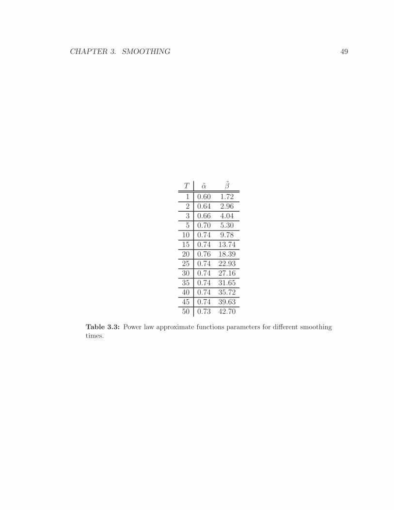
ciated single flow power law approximate value functions. Table 3.3 gives the single
flow power law function parameters for T = {1, 2, 3, 5, 10, 15, 20, 25, 30, 35, 40, 45, 50}.
(Note that the example can be easily extended to many more flows.) Each λ > 0
obtains an ADP controller (P adp, Uadp), in the (P , U) plane. Figure 3.7 shows the
ADP controllers obtained using our ADP policy (power law approximate functions).
As we would expect, higher λ values correspond to lower total average power. In the
section following we characterize ADP performance.
CHAPTER 3. SMOOTHING 49
T α β
1 0.60 1.722 0.64 2.963 0.66 4.045 0.70 5.3010 0.74 9.7815 0.74 13.7420 0.76 18.3925 0.74 22.9330 0.74 27.1635 0.74 31.6540 0.74 35.7245 0.74 39.6350 0.73 42.70
Table 3.3: Power law approximate functions parameters for different smoothingtimes.

CHAPTER 3. SMOOTHING 50
P
U
0.25 0.5 0.75 10
0.5
1
1.5
Figure 3.7: ADP controllers for 200 values in λ ∈ [0.5, 10].
3.6 Upper bound policies
In this section we describe two heuristic data flow rate policies that achieve upper
bounds for the (multi-flow) flow rate control problem (upper bounds on the optimal
objective value J⋆). These upper bounds give us a way to measure the performance
of our suboptimal flow policy ϕadp: If Jadp is close to an upper bound, then we know
that our suboptimal flow policy is nearly optimal.
3.6.1 Steady-state policy
The steady-state policy is given by
ϕss(s, gt) = argmaxft≥0
(U(s)− λPt) , (3.13)
CHAPTER 3. SMOOTHING 51
where gt is channel gain at time t, and s is the steady-state flow rate vector (indepen-
dent of time) obtained by solving the optimization problem
maximize U(s)− λφ(s,E g)
subject to s ≥ 0,
with optimization variable s, and λ known. Let J ste be our steady-state upper bound
on J⋆ obtained using the policy (3.13) to solve (3.3). Note that in the above opti-
mization problem, we ignore time (and hence, smoothing), and variations in channel
gains, and so for each λ, s is the optimal (steady-state) flow vector. (This is sometimes
called the certainty equivalent problem associated with the stochastic programming
problem [BL97, Pre95].)
By Jensen’s inequality (and convexity of the max) it is easy to see J ste is an
upper bound on J⋆. Note that once s is determined, we can evaluate (3.13) using the
water-filling algorithm described earlier.
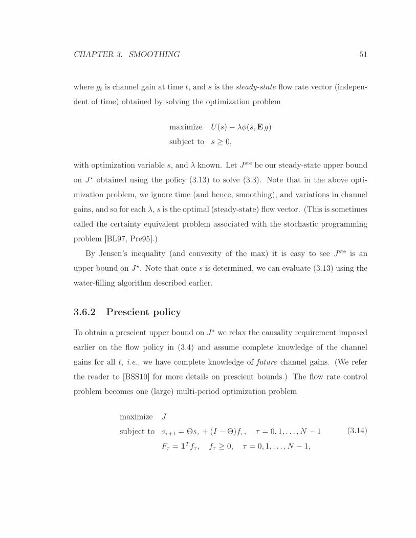
3.6.2 Prescient policy
To obtain a prescient upper bound on J⋆ we relax the causality requirement imposed
earlier on the flow policy in (3.4) and assume complete knowledge of the channel
gains for all t, i.e., we have complete knowledge of future channel gains. (We refer
the reader to [BSS10] for more details on prescient bounds.) The flow rate control
problem becomes one (large) multi-period optimization problem
maximize J
subject to sτ+1 = Θsτ + (I −Θ)fτ , τ = 0, 1, . . . , N − 1
Fτ = 1Tfτ , fτ ≥ 0, τ = 0, 1, . . . , N − 1,
(3.14)
CHAPTER 3. SMOOTHING 52
where the optimization variables are the flow rates f0, . . . , fN−1, and smoothed flow
rates s1, . . . , sN . The problem data are the initial smoothed flow rate vector s0 and
the channel gains sequence. g0, . . . , gN−1. (Note the initial smoothed flow rate vector
will not affect the computation and resulting upper bound.) This is a convex opti-
mization problem. For each channel realization, the optimal J is a random variable
(parameterized by λ) so we evaluate via Monte Carlo simulation (for large N) – solve
(3.14) for N independent realizations of the channel gains taking the mean over N as
the upper bound. We let
Jpre = Upre − λP pre,
denote our prescient upper bound on J⋆.
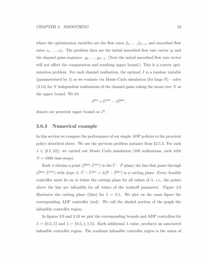
3.6.3 Numerical example
In this section we compare the performance of our simple ADP policies to the prescient
policy described above. We use the previous problem instance from §3.5.3. For each
λ ∈ [0.5, 10]), we carried out Monte Carlo simulation (100 realizations, each with
N = 1000 time-steps).
Each λ obtains a point (P pre, Upre) in the U – P plane; the line that passe through
(P pre, Upre) with slope λ: U − Upre = λ(P − P pre) is a cutting plane. Every feasible
controller must lie on or below the cutting plane for all values of λ, i.e., the points
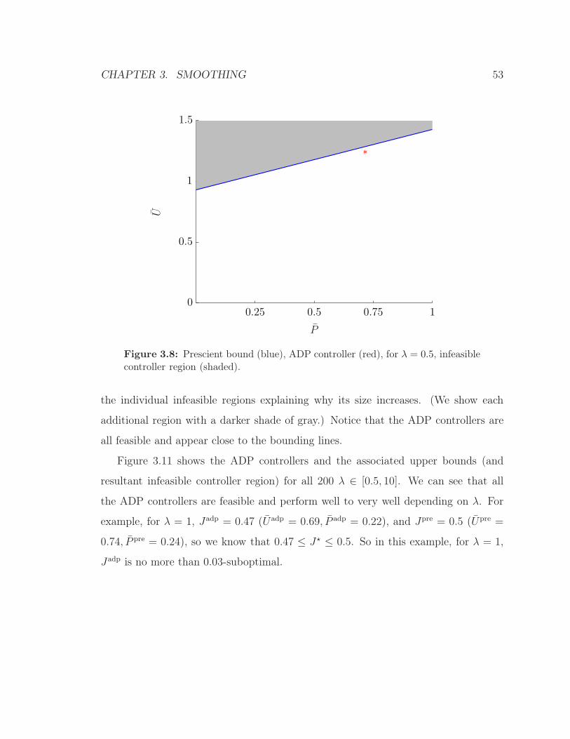
above the line are infeasible for all values of the tradeoff parameter. Figure 3.8
illustrates the cutting plane (blue) for λ = 0.5. We plot on the same figure the
corresponding ADP controller (red). We call the shaded portion of the graph the
infeasible controller region.
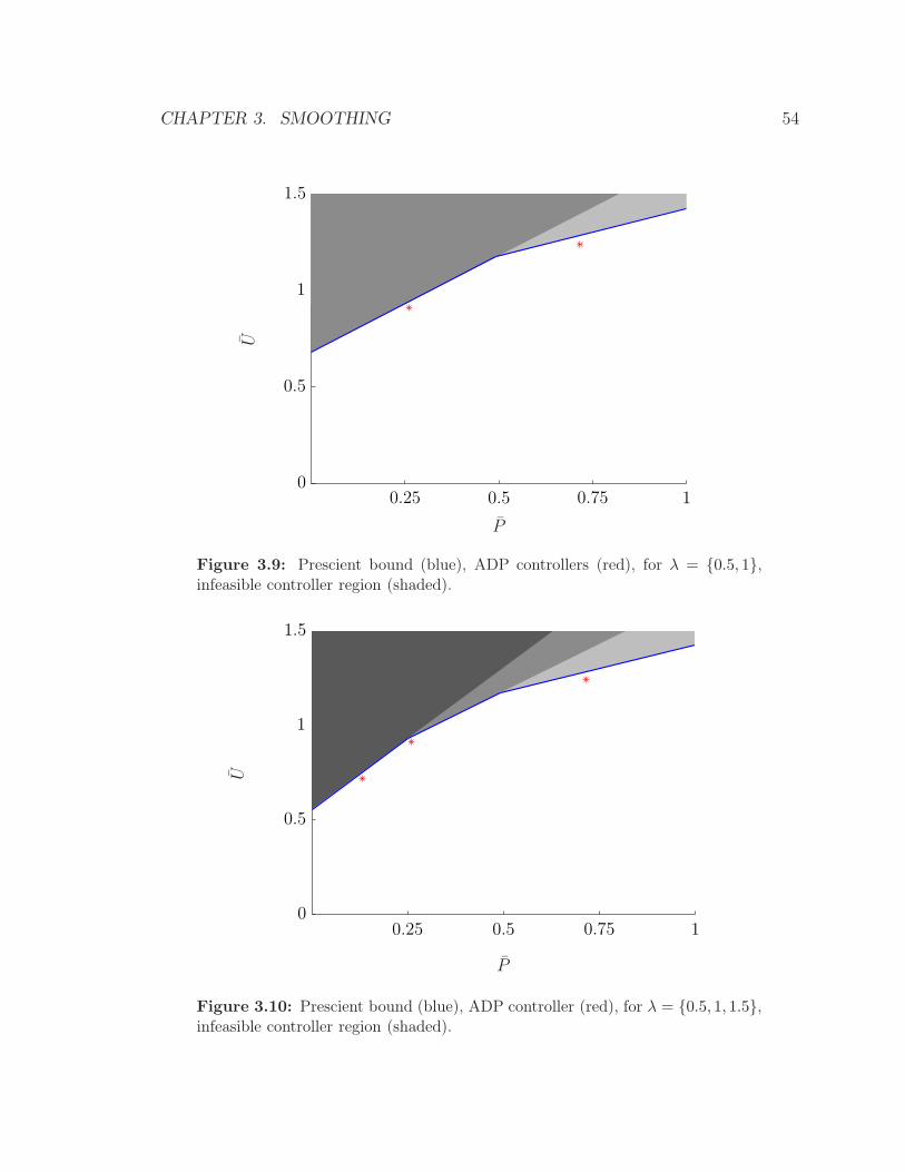
In figures 3.9 and 3.10 we plot the corresponding bounds and ADP controllers for
λ = {0.5, 1} and λ = {0.5, 1, 1.5}. Each additional λ value, produces an associated
infeasible controller region. The resultant infeasible controller region is the union of
CHAPTER 3. SMOOTHING 53
P
U
0.25 0.5 0.75 10
0.5
1
1.5
Figure 3.8: Prescient bound (blue), ADP controller (red), for λ = 0.5, infeasiblecontroller region (shaded).
the individual infeasible regions explaining why its size increases. (We show each
additional region with a darker shade of gray.) Notice that the ADP controllers are
all feasible and appear close to the bounding lines.
Figure 3.11 shows the ADP controllers and the associated upper bounds (and
resultant infeasible controller region) for all 200 λ ∈ [0.5, 10]. We can see that all
the ADP controllers are feasible and perform well to very well depending on λ. For
example, for λ = 1, Jadp = 0.47 (Uadp = 0.69, P adp = 0.22), and Jpre = 0.5 (Upre =
0.74, P pre = 0.24), so we know that 0.47 ≤ J⋆ ≤ 0.5. So in this example, for λ = 1,
Jadp is no more than 0.03-suboptimal.
CHAPTER 3. SMOOTHING 54
P
U
0.25 0.5 0.75 10
0.5
1
1.5
Figure 3.9: Prescient bound (blue), ADP controllers (red), for λ = {0.5, 1},infeasible controller region (shaded).
P
U
0.25 0.5 0.75 10
0.5
1
1.5
Figure 3.10: Prescient bound (blue), ADP controller (red), for λ = {0.5, 1, 1.5},infeasible controller region (shaded).
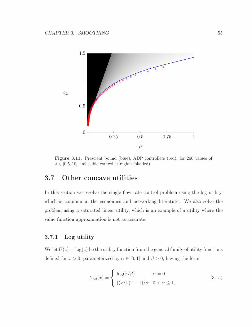
CHAPTER 3. SMOOTHING 55
P
U
0.25 0.5 0.75 10
0.5
1
1.5
Figure 3.11: Prescient bound (blue), ADP controllers (red), for 200 values ofλ ∈ [0.5, 10], infeasible controller region (shaded).
3.7 Other concave utilities
In this section we resolve the single flow rate control problem using the log utility,
which is common in the economics and networking literature. We also solve the
problem using a saturated linear utility, which is an example of a utility where the
value function approximation is not as accurate.
3.7.1 Log utility
We let U(z) = log(z) be the utility function from the general family of utility functions
defined for x > 0, parameterized by α ∈ [0, 1] and β > 0, having the form
Uαβ(x) =
log(x/β) α = 0
((x/β)α − 1)/α 0 < α ≤ 1,(3.15)

CHAPTER 3. SMOOTHING 56
where log is a special case, for α = 0. When α = 0, the effect of β is additive in the
utility, and so has no effect when maximizing utility. We use β = 1.
We consider two examples. The first flow is lightly smoothed (T = 1; θ = 0.37);
the second flow is heavily smoothed (T = 100; θ = 0.99). The channel gains gt are
IID exponential variables with mean E gt = 1. We use the power function (3.2), with
µ = 1.
We see from figure 3.12, which shows the (optimal) value functions together with
their power law approximate value functions (8.9s0.25 (light smoothing) and 192.5s0.26
(heavy smoothing)), that the approximations are very accurate. The corresponding
power law approximate policies are shown in figures 3.14 and ??. Again, we see the
same characteristics in the previous examples. We notice an even larger no-transmit
region here, which is due not only to the longer smoothing time (T = 100) but also
because of the risk-limit properties of log utility.
Average power vs average utility. Figure 3.15 shows the average power versus
average utility curves for both flows. The bottom plot illustrates further the average
power difference requirements. The average power required to generate U = −1.5
is P = 0.23 (λ = 0.2.1) for the heavily smoothed flow and P = 2.3 (λ = 0.25) for
the lightly smoothed flow. This corresponds to a 10× reduction in power for this
example.
Figure 3.16 shows sample power trajectories for both flows.
3.7.2 Saturated linear utility
In our second example we use the saturated linear utility function given by
Uαβ(x) = min(αx, β), (3.16)
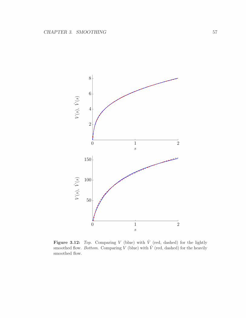
CHAPTER 3. SMOOTHING 57
s
V(s),V(s)
0 1 2
2
4
6
8
s
V(s),V(s)
0 1 2
50
100
150
Figure 3.12: Top. Comparing V (blue) with V (red, dashed) for the lightlysmoothed flow. Bottom. Comparing V (blue) with V (red, dashed) for the heavilysmoothed flow.
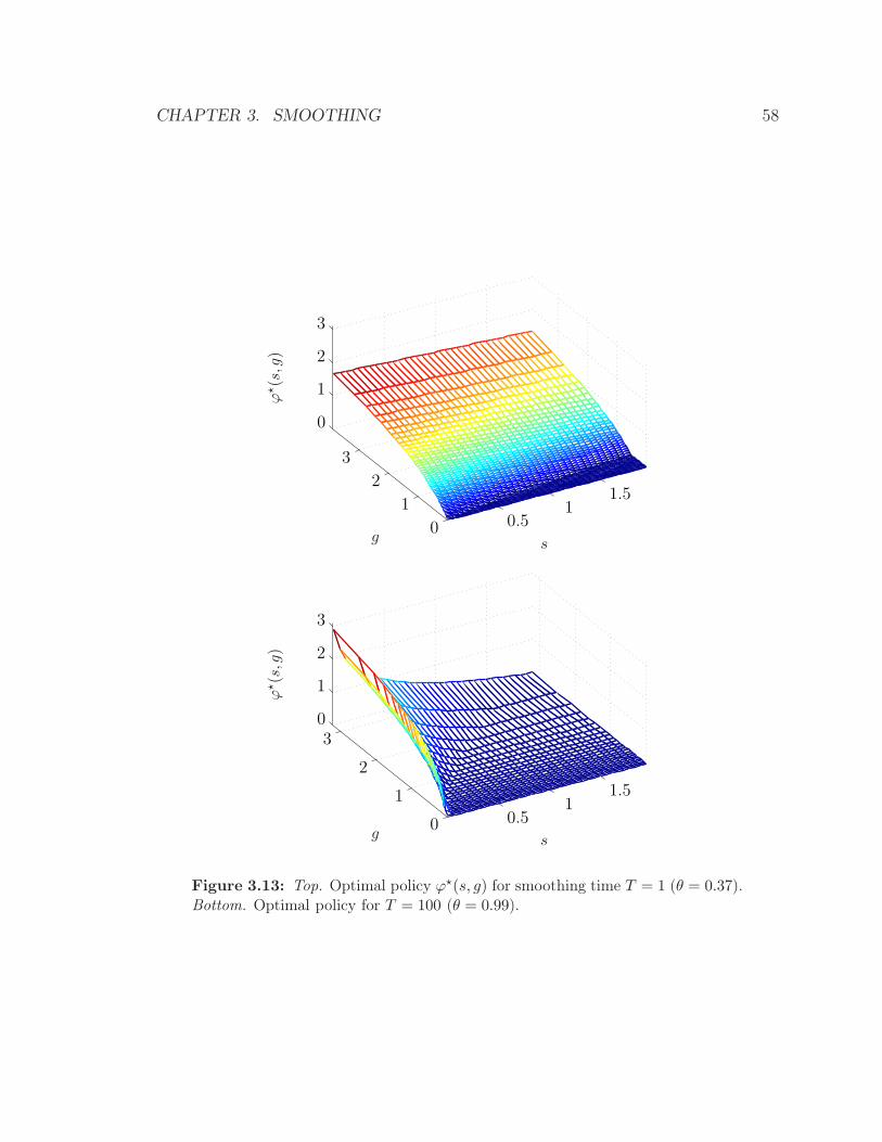
CHAPTER 3. SMOOTHING 58
g s
ϕ⋆(s,g)
0.51
1.5
0
1
2
3
0
1
2
3
g s
ϕ⋆(s,g)
0.51
1.5
0
1
2
30
1
2
3
Figure 3.13: Top. Optimal policy ϕ⋆(s, g) for smoothing time T = 1 (θ = 0.37).Bottom. Optimal policy for T = 100 (θ = 0.99).
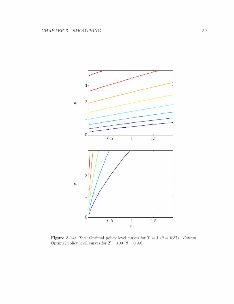
CHAPTER 3. SMOOTHING 59
g
0.5 1 1.50
1
2
3
g
s0.5 1 1.5
0
1
2
Figure 3.14: Top. Optimal policy level curves for T = 1 (θ = 0.37). Bottom.
Optimal policy level curves for T = 100 (θ = 0.99).
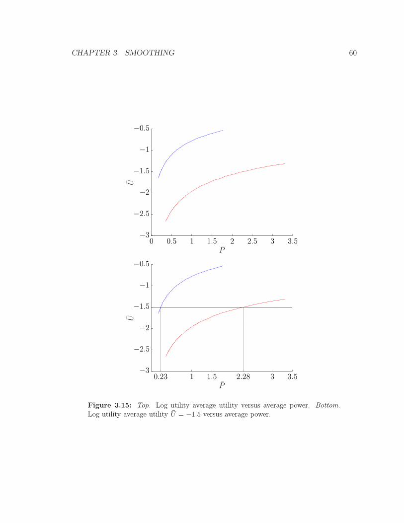
CHAPTER 3. SMOOTHING 60
U
P0 0.5 1 1.5 2 2.5 3 3.5
−3
−2.5
−2
−1.5
−1
−0.5U
P0.23 1 1.5 2.28 3 3.5
−3
−2.5
−2
−1.5
−1
−0.5
Figure 3.15: Top. Log utility average utility versus average power. Bottom.
Log utility average utility U = −1.5 versus average power.
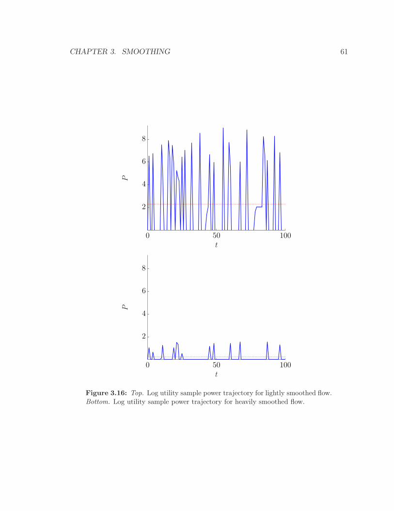
CHAPTER 3. SMOOTHING 61
P
t0 50 100
2
4
6
8
P
t0 50 100
2
4
6
8
Figure 3.16: Top. Log utility sample power trajectory for lightly smoothed flow.Bottom. Log utility sample power trajectory for heavily smoothed flow.
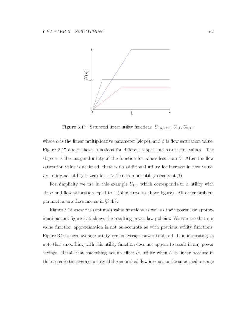
CHAPTER 3. SMOOTHING 62
0 1 20
0.5
1
U(s)
s
Figure 3.17: Saturated linear utility functions: U0.5,0.375, U1,1, U2,0.5.
where α is the linear multiplicative parameter (slope), and β is flow saturation value.
Figure 3.17 above shows functions for different slopes and saturation values. The
slope α is the marginal utility of the function for values less than β. After the flow
saturation value is achieved, there is no additional utility for increase in flow value,
i.e., marginal utility is zero for x > β (maximum utility occurs at β).
For simplicity we use in this example U1,1, which corresponds to a utility with
slope and flow saturation equal to 1 (blue curve in above figure). All other problem
parameters are the same as in §3.4.3.
Figure 3.18 show the (optimal) value functions as well as their power law approx-
imations and figure 3.19 shows the resulting power law policies. We can see that our
value function approximation is not as accurate as with previous utility functions.
Figure 3.20 shows average utility versus average power trade off. It is interesting to
note that smoothing with this utility function does not appear to result in any power
savings. Recall that smoothing has no effect on utility when U is linear because in
this scenario the average utility of the smoothed flow is equal to the smoothed average
CHAPTER 3. SMOOTHING 63
utility in the case where the utility is linear,i.e.,
Uj = (1/N)N∑
t=1
U(θjst) = (1/N)N∑
t=1
θjU(st) = U .
3.8 Alternative evaluation of ADP policy
We describe in this section an interior point method that exploits the problem struc-
ture also yielding a very efficient solution method for the ADP flow rate policy, i.e.,
solving (3.12); see, e.g., [MBL10]. Recall the optimization problem
maximize V adp(Θs+ (I −Θ)f)− λφ(F, g)
subject to F = 1Tf, fj ≥ 0, j = 1, . . . , n.
We describe a barrier method. Let us first make some simplifying substitutions to
our problem definition. We can rewrite (3.12) as
maximize U(y)
subject to Ay = 0, yj ≥ 0, j = 1, . . . , n,
where
y = (f, F )
U(y) = V adp(Θs+ (I −Θ)f)− λφ(F, g)
A = (1, . . . , 1,−1)T .
Suppose y⋆ is the minimizing point of (3.12), which we assume exists, we solve for
y⋆ by computing a sequence of points y(k), k = 1, . . ., where y(k+1) = y(k) + t(k)∆y(k)
except when y(k) = y⋆, i.e., y(k) is optimal. The critical step is computing the update
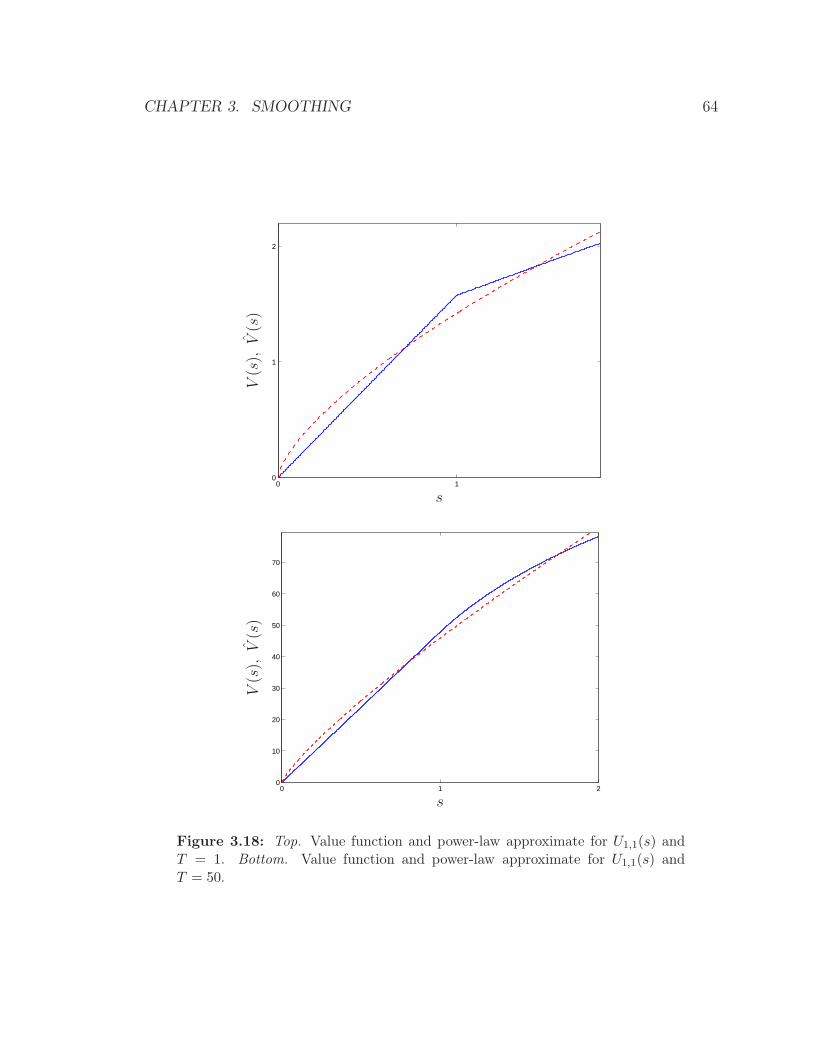
CHAPTER 3. SMOOTHING 64
0 10
1
2
s
V(s),V(s)
0 1 20
10
20
30
40
50
60
70
s
V(s),V(s)
Figure 3.18: Top. Value function and power-law approximate for U1,1(s) andT = 1. Bottom. Value function and power-law approximate for U1,1(s) andT = 50.
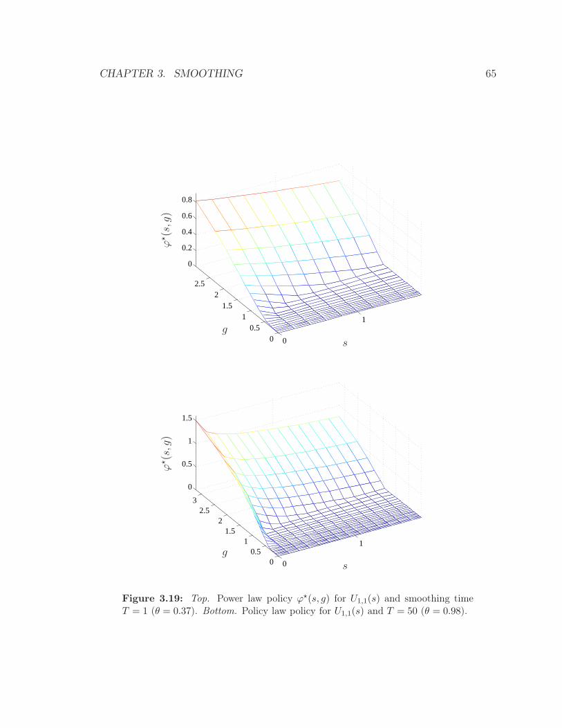
CHAPTER 3. SMOOTHING 65
0
1
00.5
11.5
22.5
0
0.2
0.4
0.6
0.8
gs
ϕ⋆(s,g)
0
1
00.5
11.5
22.5
3
0
0.5
1
1.5
gs
ϕ⋆(s,g)
Figure 3.19: Top. Power law policy ϕ⋆(s, g) for U1,1(s) and smoothing timeT = 1 (θ = 0.37). Bottom. Policy law policy for U1,1(s) and T = 50 (θ = 0.98).
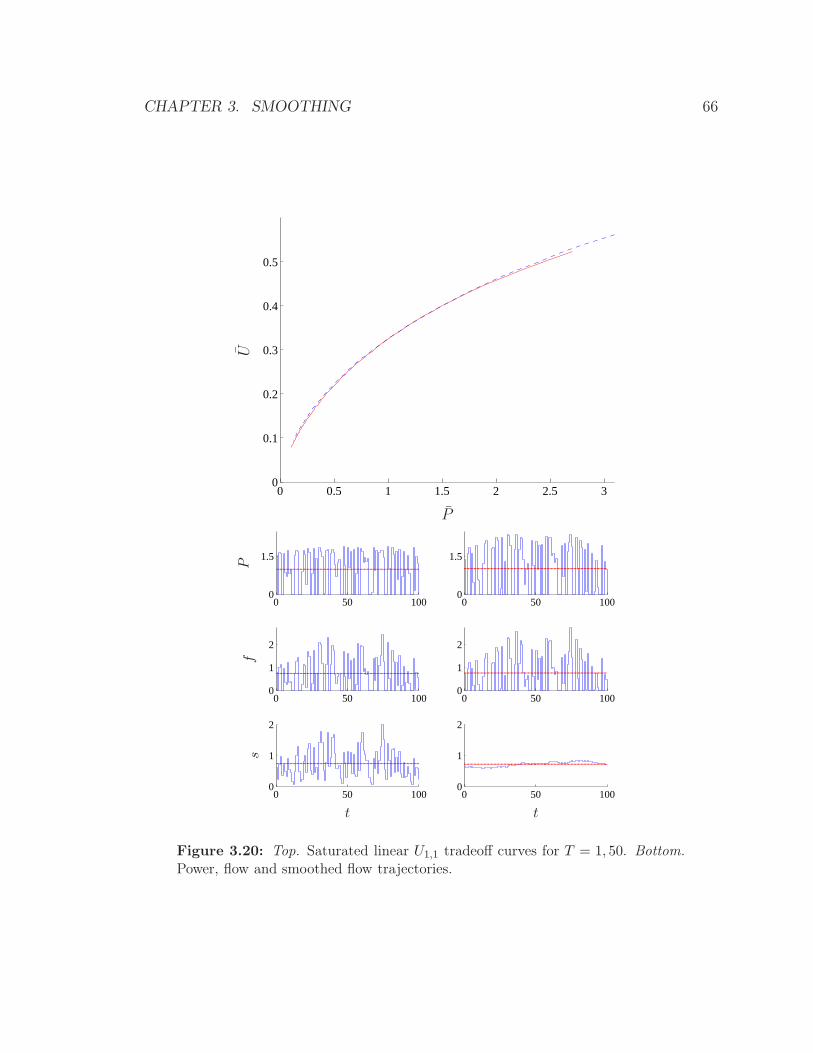
CHAPTER 3. SMOOTHING 66
0 0.5 1 1.5 2 2.5 30
0.1
0.2
0.3
0.4
0.5
P
U
0 50 1000
1.5
0 50 1000
1.5
0 50 1000
1
2
0 50 1000
1
2
0 50 1000
1
2
0 50 1000
1
2
P
tt
sf
Figure 3.20: Top. Saturated linear U1,1 tradeoff curves for T = 1, 50. Bottom.
Power, flow and smoothed flow trajectories.
CHAPTER 3. SMOOTHING 67
t(k)∆y(k) which includes a scalar step length t(k) > 0, and a search direction (or step)
∆y(k). We compute the step length using a backtracking line search [BV04, §9] and
the search direction using Newton’s method [BV04, §9].
Logarithmic barrier. Barrier methods allow us to approximate inequality con-
strained problems as equality constrained problems to which we can apply standard
iteration algorithms. We use a logarithmic barrier function, i.e., we replace the in-
equality constraints with −(1/t)∑n
j=1 log fj where t > 0 is a parameter that sets the
accuracy of the approximation. We let ψ(y) =∑n
j=1 log fj giving the approximation
minimize −U(y)− (1/t)ψ(y)
subject to Ay = 0, yj ≥ 0, j = 1, . . . , n,(3.17)
with optimization variables yj, j = 1, . . . , n+1. For t > 0, the objective is convex and
so (3.17) is a convex optimization problem and the solution defined as y⋆(t) (assuming
it exists) is unique. (The approximation gets better as t increases).
Optimality conditions Using the dual variable ν ∈ R we can write the optimality
conditions for the approximate problem as
Ay⋆ = 0, fj ≥ 0, j = 1, . . . , n
λj ≥ 0, j = 1, . . . , n
−∇U(y⋆) +∑n
j=1λj∇ψ(y
⋆) + ATν⋆ = 0
−λjfj = 1/t, j = 1, . . . , n.
Newton method. Since the objective in (3.17) is twice differentiable we calculate
the search direction using Newton’s method. (We assume that the necessary technical
conditions hold). The primal Newton step, ∆y and the associated dual Newton step,
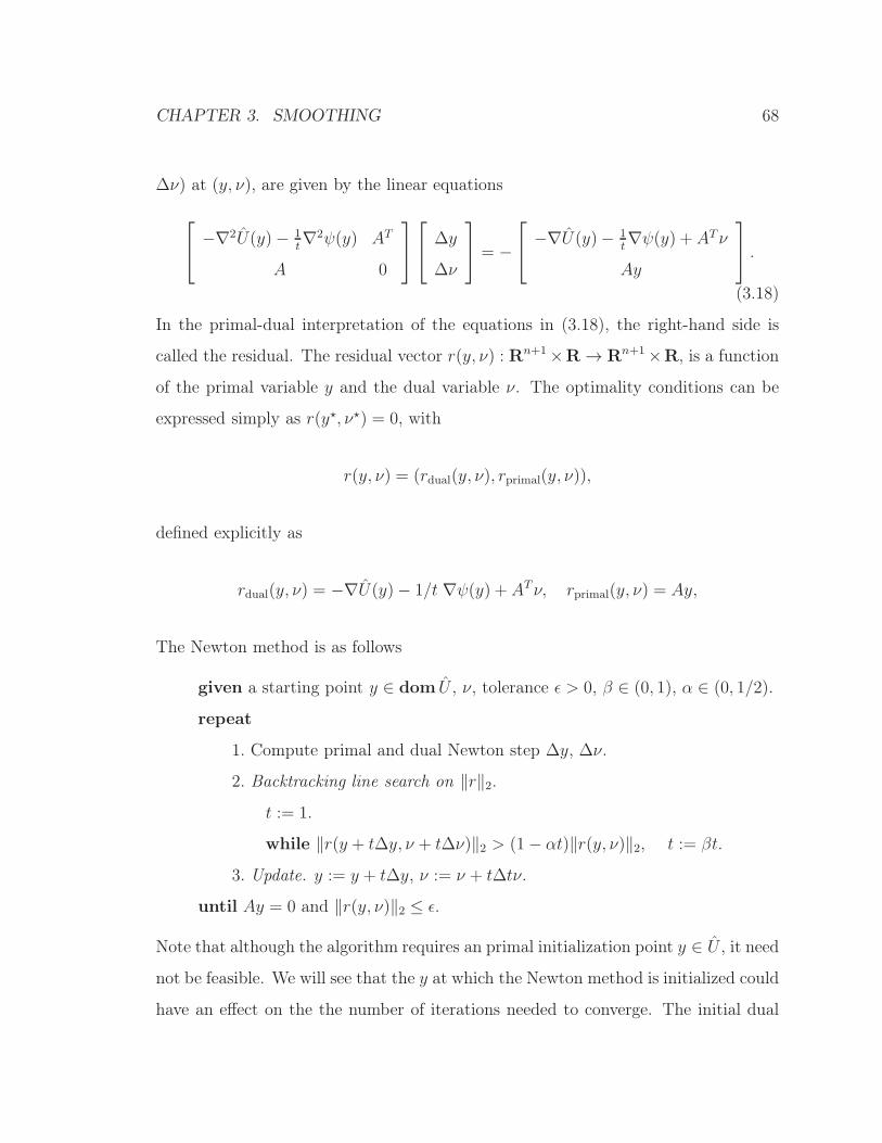
CHAPTER 3. SMOOTHING 68
∆ν) at (y, ν), are given by the linear equations
−∇2U(y)− 1t∇2ψ(y) AT
A 0
∆y
∆ν
= −
−∇U (y)− 1t∇ψ(y) + ATν
Ay
.
(3.18)
In the primal-dual interpretation of the equations in (3.18), the right-hand side is
called the residual. The residual vector r(y, ν) : Rn+1×R → Rn+1×R, is a function
of the primal variable y and the dual variable ν. The optimality conditions can be
expressed simply as r(y⋆, ν⋆) = 0, with
r(y, ν) = (rdual(y, ν), rprimal(y, ν)),
defined explicitly as
rdual(y, ν) = −∇U(y)− 1/t ∇ψ(y) + ATν, rprimal(y, ν) = Ay,
The Newton method is as follows
given a starting point y ∈ dom U , ν, tolerance ǫ > 0, β ∈ (0, 1), α ∈ (0, 1/2).
repeat
1. Compute primal and dual Newton step ∆y, ∆ν.
2. Backtracking line search on ‖r‖2.
t := 1.
while ‖r(y + t∆y, ν + t∆ν)‖2 > (1− αt)‖r(y, ν)‖2, t := βt.
3. Update. y := y + t∆y, ν := ν + t∆tν.
until Ay = 0 and ‖r(y, ν)‖2 ≤ ǫ.
Note that although the algorithm requires an primal initialization point y ∈ U , it need
not be feasible. We will see that the y at which the Newton method is initialized could
have an effect on the the number of iterations needed to converge. The initial dual
CHAPTER 3. SMOOTHING 69
value ν, however, does not affect algorithm performance.
Forming and solving the KIT system. In practice, the main drawback of the
Newton method is the cost of forming the Hessian (top left block) of the KKT matrix
in equation (3.18) and solving for the newton step: ∆y and ∆ν. In our problem, we
show that we can exploit the special structure of the KKT system to compute the
Newton step in O(n) time instead of O(n3) time of a generic matrix inversion.
We let d ∈ Rn+1 be the gradient of the objective in (3.17), i.e.,
d = −∇U (y)− 1/t ∇ψ(y),
to get
dj = −Kjαj(1− θj)(θjsj + (1− θj)yj)αj−1 −
1
tyj, j = 1, . . . , n, dn+1 =
exp(yn+1)
g.
We let H be the Hessian, i.e.,
H = −∇2U(y)−1
t∇2ψ(y),
with
H =
H1
. . .
Hn
Hn+1
,
where
Hj = −Kj(α2j − α)(1− θj)
2(θ1sj + (1− θj)yj)αj−2 + 1/(ty2j ), j = 1, . . . , n,
CHAPTER 3. SMOOTHING 70
and
Hn+1 = exp(yn+1)/g.
Let g = g + AT ν and h = Ay, we can write (3.18) as
H AT
A 0
∆y
∆ν
= −
g
h
.
It is easy to see that H is positive definite, i.e., H ≻ 0, and so we can solve the system
of equations via block elimination:
∆ν = −(AH−1AT )−1(h− AH−1g), ∆y = H−1(g − AT∆ν).
The cost of the elimination method is summarized as follows.
1. Invert H (n operations, since H is diagonal).
2. Invert AH−1AT (n operations, AT ∈ Rn+1, AH−1AT ∈ R).
3. Evaluate (AH−1AT )−1(h−AH−1g) (n operations).
4. Evaluate H−1(g − AT∆ν) (n operations).
The total cost therefore is O(n).
3.9 Conclusion
In this chapter we present a variation on a multi-period stochastic network utility
maximization problem as a constrained convex stochastic control problem. We show
that judging flow utilities dynamically, i.e., with a utility function and a smoothing
time scale, is a good way to account for network applications with heterogeneous rate
demands.
CHAPTER 3. SMOOTHING 71
For the case of a single flow, our numerically computed value functions obtain
flow policies that optimally trade-off average utility and average power. We show
that simple power law functions are reasonable approximations of the optimal value
functions, and that these simple functions obtain near optimal performance.
For the case of multiple flows on a single link (where the value function is not prac-
tically computable using dynamic programming), we approximate the value function
with a combination of the simple one-dimensional power law functions. Simulations,
and comparison with upper bounds on the optimal value, show that the resulting
ADP policy can obtain very good performance.
Chapter 4
Queue-Length-Based 2-Hop Rate
Control
In this chapter we consider a simple variation to the flow rate control problem from
§3.2.3, where we have a relay node (buffer), through which flows traverse from source
(transmitter) to destination (receiver). We consider the problem of choosing the
data flow rates on the (two) wireless links with randomly varying channel gains to
optimally trade off average utility of the instantaneous data flow rate at the receiver
and the average system costs. Cost consists of the average transmit power costs on the
wireless links and average costs incurred at the relay node. We pose the problem as
a convex stochastic control problem with linear dynamics. Using stochastic dynamic
programming, we show the effect of different utility and cost functions on flow rates
and buffer occupancy. We illustrate our results via numerical examples.
4.1 Background
Throughput-optimal scheduling based on queue-length, backpressure, and differen-
tial backlog algorithms are introduced in [TE92] have been widely extended and
72

CHAPTER 4. 2-HOP 73
now include fair scheduling algorithms also based on queue-length and elastic traf-
fic sources [ES07, Sto05, NML08, ES07, GNT06]. Cross-layer network optimization
[OGB08a, SS07], decomposition [CLCD07, PC06], and distributed [LR07, PC06], so-
lution methods have also been employed for these problems.
Our setup includes cross-layer optimization via channel-aware utility maximiza-
tion. We augment the (known) queue-length information with the random channel
gains as the system state variable for our causal feedback data flow rate control policy.
4.2 Network description
(ft)11 (ft)21
(ft)1n (ft)2n
qt
Figure 4.1: Single-hop network.
A wireless network comprised of one transmitter, one relay, and one receiver sup-
ports n data flows across m wireless channels that vary with time. Network time is
modeled using discrete-time intervals t = 0, 1, . . .. The relay contains a buffer where
a queue is maintained for each data flow in the network. In this simple problem
setup there are m = 2 (by construction), wireless links: the first link supports traffic
between the transmitter and the relay node, and the second link supports traffic be-
tween the relay and the receiver as shown in figure 4.1. We let Ft ∈ Rm×n denote the
flow rate matrix where (ft)ij is the flow rate on link i, for flow j, at time t. We let
(ft)i ∈ Rn+ (the ith row of Ft) be the vector of flow rates on link i. We let f (j)
t ∈ Rm+
CHAPTER 4. 2-HOP 74
(the jth column of Ft) be the vector of flow rates associated with flow j.
4.2.1 Average utility
Network utility is associated with the flow rate delivered at the receiver. In the single-
hop configuration therefore, this corresponds to the utility derived on the link from
relay to receiver, i.e., the second wireless link. At each time t the link utility is given
by
U(ft)2 = U1(ft)21 + · · ·+ Un(ft)2n.
The overall average utility is given by
U = limN→∞
E1
N
N−1∑
t=0
U(ft)2,
where we assume that the expectation exists. We take the utility functions Uj, j =
1, . . . , n, to be concave nondecreasing differentiable functions. Network satisfaction is
thus derived only as a result of packets delivered to the (destination) receiver. (There
is no direct utility for the intermediate transmission from source to relay.) Total
average utility is separable across flows.
4.2.2 Average cost
Average power cost. The flow rates will depend on the random channel gains
associated with the time varying wireless channel and so are random variables. We
let gt ∈ Rm++ denote the channel gain vector, where at time t, (gt)i is the channel
gain parameter on link i; we assume that (gt)i are independent identically distributed
(IID) random variables, with known distribution. In general wireless links in near
proximity interfere with each other and the link gains are therefore correlated. We
choose here to assume independence for simplicity of our problem setup. At each

CHAPTER 4. 2-HOP 75
time t, let Tt ∈ Rm+ denote the total flow rate vector where
(Tt)i = (ft)i1+, · · · ,+(ft)in,
is the total flow on link i. The power required to support Tt (and the corresponding
network flow rate matrix) is given by
Pt = ψ(Tt, gt),
where
ψ(Tt, gt) =m∑
i=1
ψi((Tt)i, (gt)i),
where ψi is convex and increasing in (Tt)i. The total average power is
P = limN→∞
E1
N
N−1∑
t=0
Pt.
The total average power is separable in the links (flow rate vectors) but not necessarily
separable in the flows.
Average queue cost. The relay maintains n queues, one for each flow. We let
qt ∈ Rn+ denote the queue length vector where at time t, (qt)j is the value of the jth
queue. The jth queue evolves according to the linear dynamical system
(qt+1)j = (qt)j + Af(j)t , A =
[
1 −1]
, j = 1, . . . , n
where A describes the queue balance equation. We impose a queue maintenance
cost, which encourages transmission when feasible from the relay to the receiver. The
queue cost also discourages the queue lengths from growing unbounded. At time t,
CHAPTER 4. 2-HOP 76
the total queue cost is given by Ct = χ(qt), where
χ(qt) =
n∑
j=1
χj(qt)j,
and χj are strictly convex and increasing in queue length. The total average queue
maintenance cost is
C = limN→∞
E1
N
N−1∑
t=0
Ct.
The total average queue cost is separable across the flows.
4.2.3 Flow constraints
We require that flow rates are nonnegative for all t. We require also that the queue
lengths are nonnegative: At any time t, the flow rates assigned on link 2 must be less
than or equal to the associated queue lengths from the previous time period t − 1,
i.e., at any time t, you can not assign more rate than was in the buffer at time t− 1.
Let Ct denote the set of feasible flow rates at each time t. We get
Ct = {(ft)ij | (ft)ij ≥ 0, (qt−1)j − (ft)2j ≥ 0, i = 1, 2, j = 1, . . . , n}.
Roughly, we can summarize the constraint set as follows. The channel gains on link 1
drive the flow rates on the link and consequently the queue lengths. Queue size and
link 2 channel gains directly determine network utility.

CHAPTER 4. 2-HOP 77
4.2.4 2-hop flow control problem
The overall objective is to maximize a weighted difference between average utility,
and average costs. The objective is given by
J = U − λ(P + C), (4.1)
where λ is a tradeoff parameter between average utility and average cost. At each
time t, we know the previous flow rates, and the current and previous queue lengths
and channel gains. We wish to find a stationary flow rate control policy, i.e., function
ϕ : Rn+ ×Rn
+ × Rm++ → Rm×n
+ ,
with
Ft = ϕ(st, qt, gt), t = 0, 1, . . . ,
such that the constraints are satisfied at each time t, i.e., Ft ∈ Ct.
The flow rate control problem is to choose the flow rate policy ϕ to maximize the
overall objective in (4.1) while satisfying the flow rate constraints. This is a standard
convex stochastic control problem, with linear dynamics.
4.3 Optimal policy
The optimal policy is characterized by
ϕ⋆(q, g) = argmaxC
(
V (qT + Aw)− λψ(T, g))
(4.2)
CHAPTER 4. 2-HOP 78
where V : Rn → R is the Bellman (relative) value function. The value function (and
optimal value) is characterized via the fixed point equation
J⋆ + V = T V,
where for any function S : Rn+ → R, the Bellman operator T is given by
(T S)(z) = U(w2) + E
(
maxW∈C
(
S(qT + Aw2)− λψ(T, g))
)
,
where the expectation is over g. The fixed point equation and Bellman operator are
invariant under adding a constant; that is, we have T (S + a) = T S + a, for any
constant (function) a, and similarly, V satisfies the fixed point equation if and only
if V + a does. So without loss of generality we can assume that V (0) = 0. Similar
to §3.3.3 the value function can be found by value iteration [Bla62, Der66, Der70,
Sen96, Ber98, Ber05, Ber07], i.e., repeated application of the Bellman operator until
the value function converges.
Notice that the value function is a function only of the queue length vector q (not
smoothed flow). As a result, the monotonicity property from §3.3.3 no longer applies.
We can see why this is true using a simple proof by contradiction: Infinitely long
queues are undesirable for our problem.

CHAPTER 4. 2-HOP 79
4.4 One flow
Consider a simple scenario with one flow (n = 1). To simplify notation we let qt =
(qt)1 and ft = ((ft)1, (ft)2), as shown in figure 4.2, (qt ∈ R, and ft ∈ R2.) The queue
(ft)1 (ft)2
qt
Figure 4.2: Single hop, single flow.
length update is given by
qt+1 = qt + Aft,
with constraint set
C = {f | f1 ≥ 0, f2 ≥ 0, q − f2 ≥ 0}.
The value function characterized by
V (q) = E
(
maxf∈C
(U(f2) + V (q + Af)− λ(χ(q) + ψ(f, g)))
)
,
and the optimal policy is given by
ϕ⋆(q, g) = argmaxw∈C
(V (q + Aw)− λψ(w, g)) .

CHAPTER 4. 2-HOP 80
We can evaluate the optimal policy by solving an optimization problem. At each time
t, we must solve problem
maximize V (q + Af)− λψ(f, g)
subject to f1 ≥ 0, f2 ≥ 0, q − f2 ≥ 0,(4.3)
where the optimization variable is f = (f1, f2). Similar to the case of one dimension
in the previous chapter, we can compute the value function easily using using value
iteration and gridding. For concave utility and convex cost, we know that V is a
concave function and so (4.3) is a convex optimization problem.
4.4.1 Approximate policy
Since V is concave, and satisfies V (0) = 0, we can find a reasonable analytic approx-
imation, say V , using a mixture of power and polynomial (typically degree M < 3)
functions. Our approximate function V is given by
V (z) = kzα +
M∑
p=1
cpzp,
with α ∈ (0, 1). The approximate policy is given by
ϕ(q, g) = argmaxw∈C
(
V (q + Aw)− λψ(w, g))
.
4.5 Numerical Examples
In this section we give numerical examples. We take utility U(z) = z1/2 and we use
function ψi(fi, gi) = (efi − 1)/gi, to represent the power required to support flow on
link i. We take the channel gains to be exponentially distributed with E gt = (1, 1),
i.e., channel gains on each link are exponentially distributed random variables with
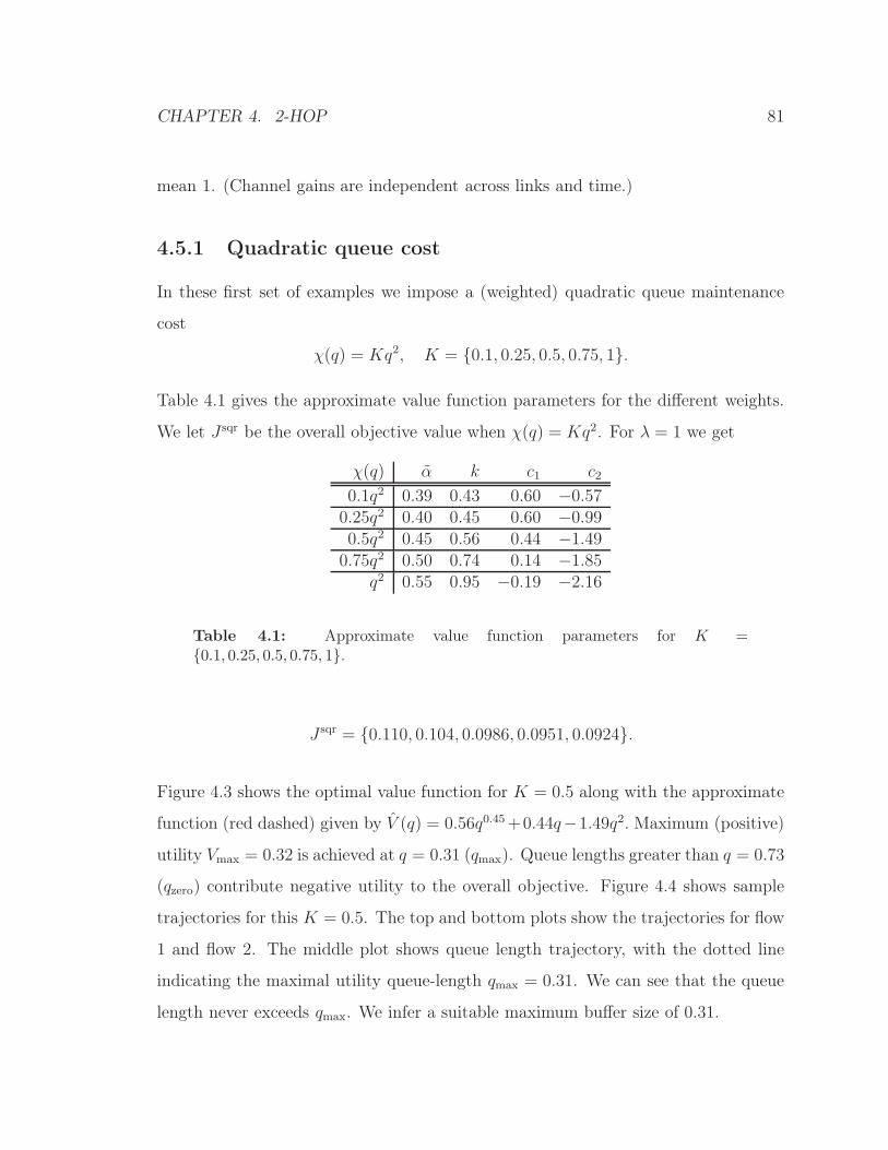
CHAPTER 4. 2-HOP 81
mean 1. (Channel gains are independent across links and time.)
4.5.1 Quadratic queue cost
In these first set of examples we impose a (weighted) quadratic queue maintenance
cost
χ(q) = Kq2, K = {0.1, 0.25, 0.5, 0.75, 1}.
Table 4.1 gives the approximate value function parameters for the different weights.
We let J sqr be the overall objective value when χ(q) = Kq2. For λ = 1 we get
χ(q) α k c1 c2
0.1q2 0.39 0.43 0.60 −0.570.25q2 0.40 0.45 0.60 −0.990.5q2 0.45 0.56 0.44 −1.490.75q2 0.50 0.74 0.14 −1.85
q2 0.55 0.95 −0.19 −2.16
Table 4.1: Approximate value function parameters for K ={0.1, 0.25, 0.5, 0.75, 1}.
J sqr = {0.110, 0.104, 0.0986, 0.0951, 0.0924}.
Figure 4.3 shows the optimal value function for K = 0.5 along with the approximate
function (red dashed) given by V (q) = 0.56q0.45+0.44q−1.49q2. Maximum (positive)
utility Vmax = 0.32 is achieved at q = 0.31 (qmax). Queue lengths greater than q = 0.73
(qzero) contribute negative utility to the overall objective. Figure 4.4 shows sample
trajectories for this K = 0.5. The top and bottom plots show the trajectories for flow
1 and flow 2. The middle plot shows queue length trajectory, with the dotted line
indicating the maximal utility queue-length qmax = 0.31. We can see that the queue
length never exceeds qmax. We infer a suitable maximum buffer size of 0.31.
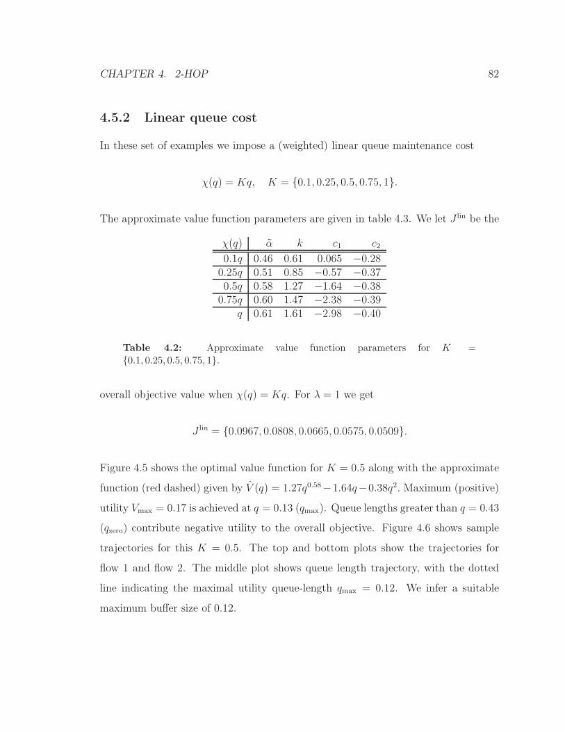
CHAPTER 4. 2-HOP 82
4.5.2 Linear queue cost
In these set of examples we impose a (weighted) linear queue maintenance cost
χ(q) = Kq, K = {0.1, 0.25, 0.5, 0.75, 1}.
The approximate value function parameters are given in table 4.3. We let J lin be the
χ(q) α k c1 c2
0.1q 0.46 0.61 0.065 −0.280.25q 0.51 0.85 −0.57 −0.370.5q 0.58 1.27 −1.64 −0.380.75q 0.60 1.47 −2.38 −0.39
q 0.61 1.61 −2.98 −0.40
Table 4.2: Approximate value function parameters for K ={0.1, 0.25, 0.5, 0.75, 1}.
overall objective value when χ(q) = Kq. For λ = 1 we get
J lin = {0.0967, 0.0808, 0.0665, 0.0575, 0.0509}.
Figure 4.5 shows the optimal value function for K = 0.5 along with the approximate
function (red dashed) given by V (q) = 1.27q0.58−1.64q−0.38q2. Maximum (positive)
utility Vmax = 0.17 is achieved at q = 0.13 (qmax). Queue lengths greater than q = 0.43
(qzero) contribute negative utility to the overall objective. Figure 4.6 shows sample
trajectories for this K = 0.5. The top and bottom plots show the trajectories for
flow 1 and flow 2. The middle plot shows queue length trajectory, with the dotted
line indicating the maximal utility queue-length qmax = 0.12. We infer a suitable
maximum buffer size of 0.12.
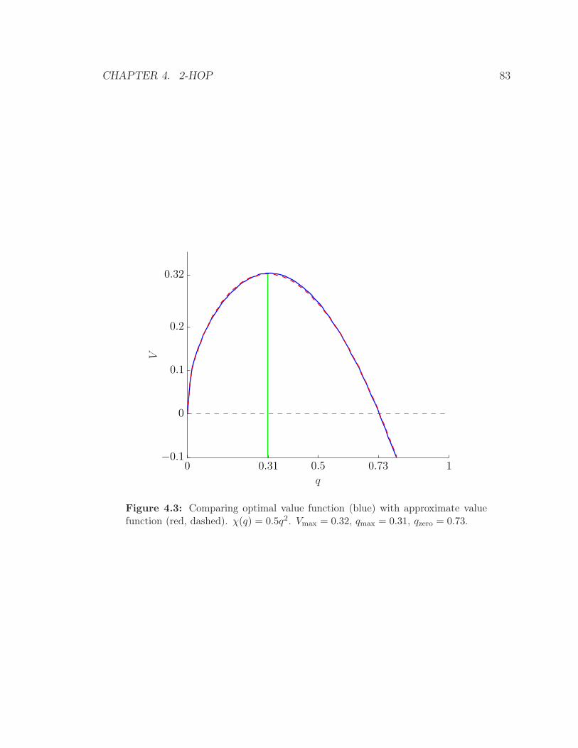
CHAPTER 4. 2-HOP 83
q
V
0 0.31 0.5 0.73 1−0.1
0
0.1
0.2
0.32
Figure 4.3: Comparing optimal value function (blue) with approximate valuefunction (red, dashed). χ(q) = 0.5q2. Vmax = 0.32, qmax = 0.31, qzero = 0.73.
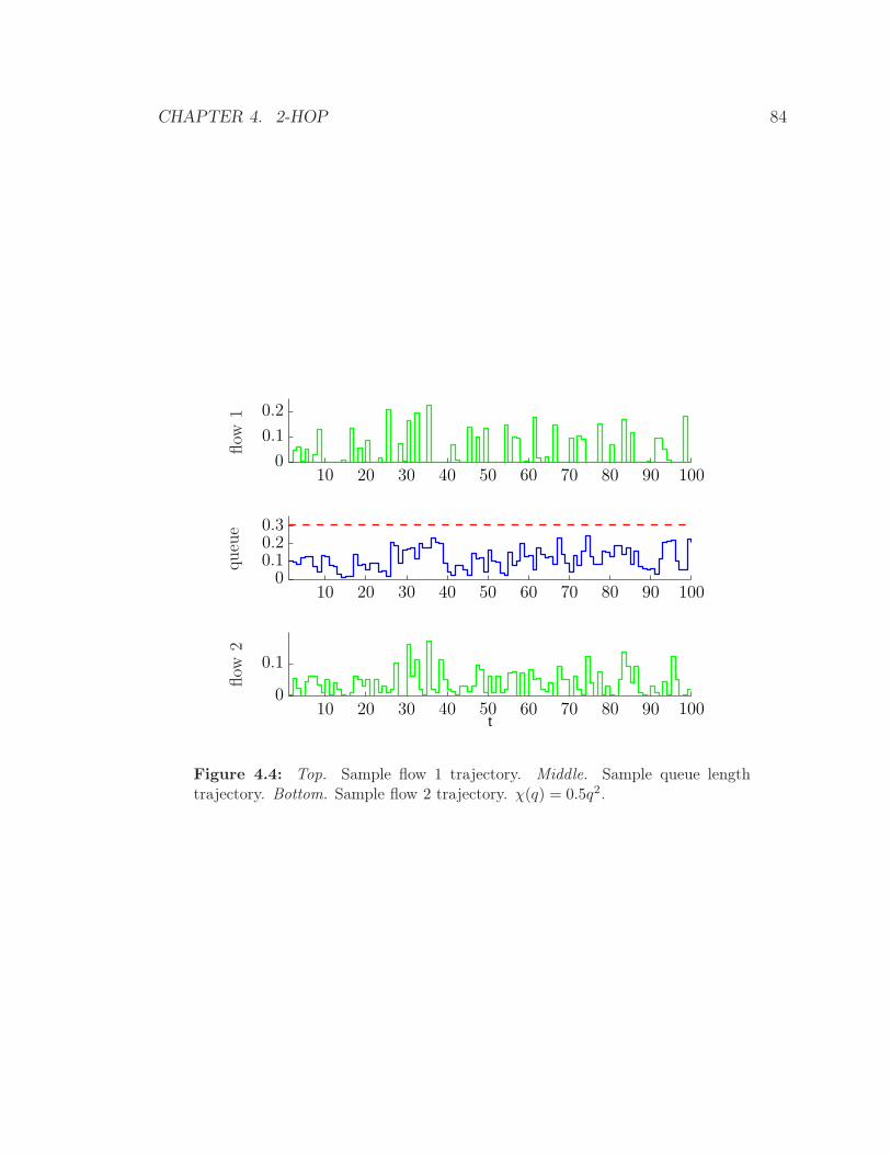
CHAPTER 4. 2-HOP 84
t
queue
flow
1flow
2
10 20 30 40 50 60 70 80 90 100
10 20 30 40 50 60 70 80 90 100
10 20 30 40 50 60 70 80 90 100
0
0.1
00.10.20.3
0
0.1
0.2
Figure 4.4: Top. Sample flow 1 trajectory. Middle. Sample queue lengthtrajectory. Bottom. Sample flow 2 trajectory. χ(q) = 0.5q2.
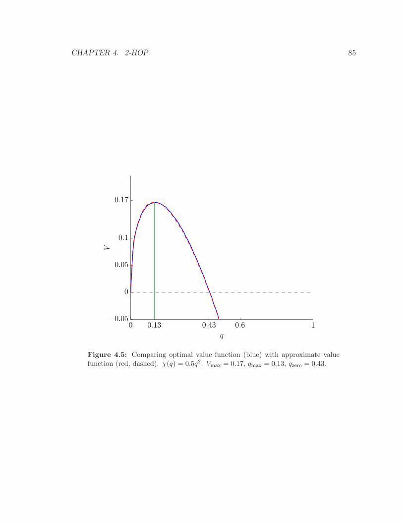
CHAPTER 4. 2-HOP 85
q
V
0 0.13 0.43 0.6 1−0.05
0
0.05
0.1
0.17
Figure 4.5: Comparing optimal value function (blue) with approximate valuefunction (red, dashed). χ(q) = 0.5q2. Vmax = 0.17, qmax = 0.13, qzero = 0.43.
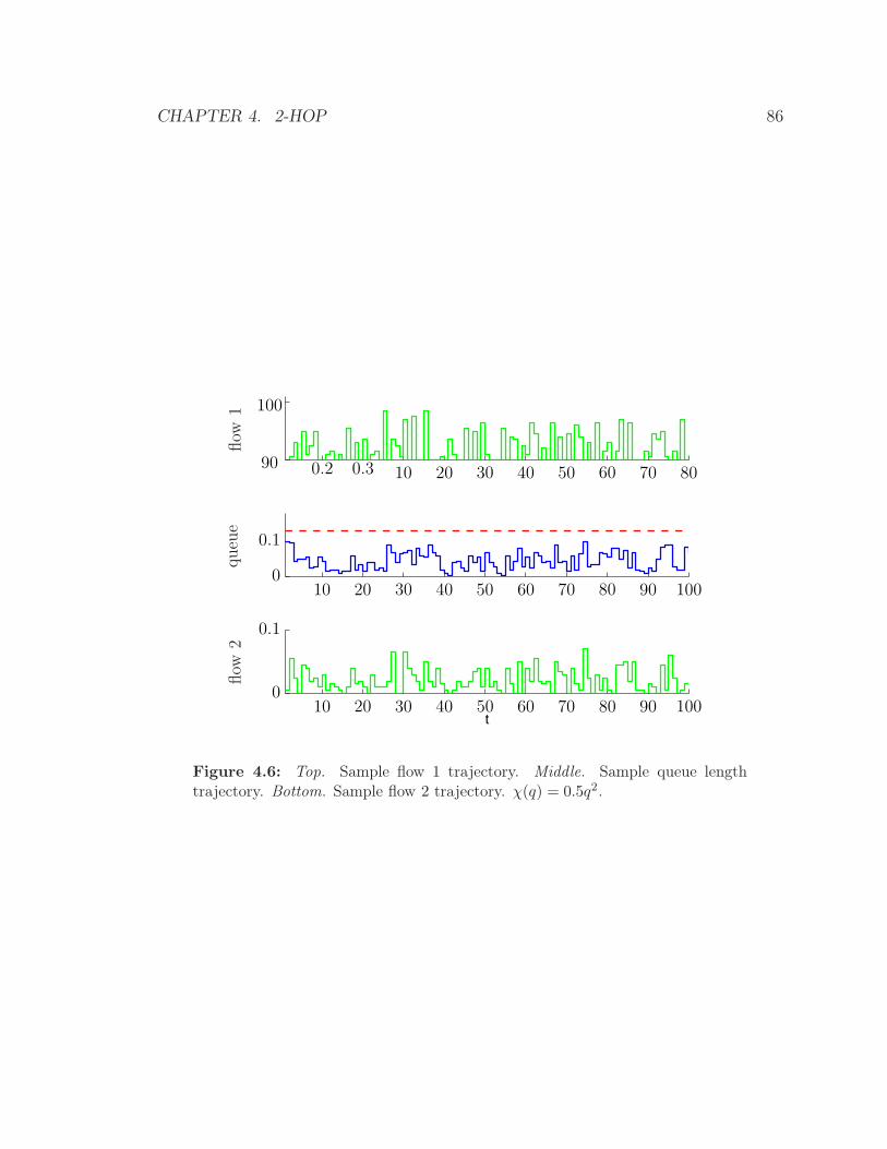
CHAPTER 4. 2-HOP 86
t
queue
flow
1flow
2
10 20 30 40 50 60 70 80 90 100
10 20 30 40 50 60 70 80 90 100
10 20 30 40 50 60 70 8090
100
0
0.1
0
0.1
0.2 0.3
Figure 4.6: Top. Sample flow 1 trajectory. Middle. Sample queue lengthtrajectory. Bottom. Sample flow 2 trajectory. χ(q) = 0.5q2.
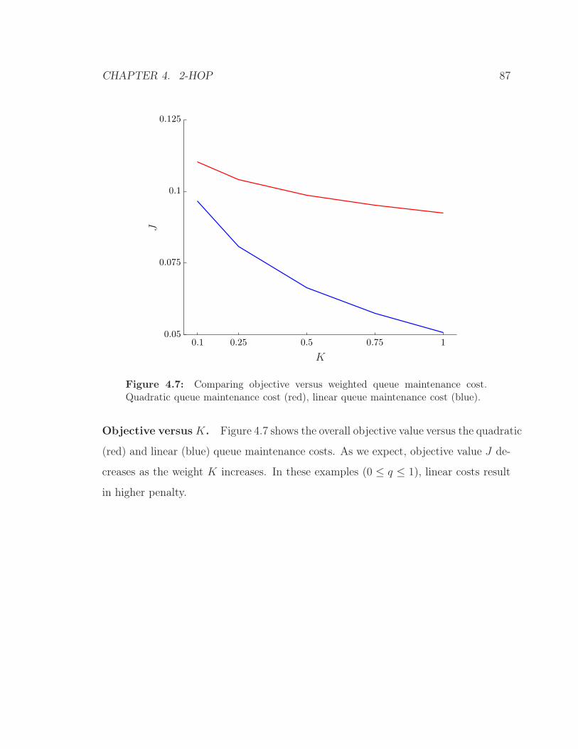
CHAPTER 4. 2-HOP 87
J
K
0.1 0.25 0.5 0.75 10.05
0.075
0.1
0.125
Figure 4.7: Comparing objective versus weighted queue maintenance cost.Quadratic queue maintenance cost (red), linear queue maintenance cost (blue).
Objective versus K. Figure 4.7 shows the overall objective value versus the quadratic
(red) and linear (blue) queue maintenance costs. As we expect, objective value J de-
creases as the weight K increases. In these examples (0 ≤ q ≤ 1), linear costs result
in higher penalty.
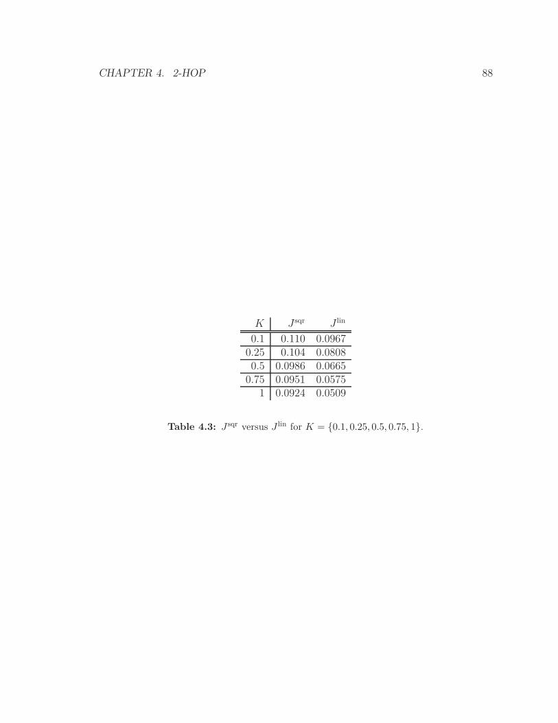
CHAPTER 4. 2-HOP 88
K J sqr J lin
0.1 0.110 0.09670.25 0.104 0.08080.5 0.0986 0.06650.75 0.0951 0.0575
1 0.0924 0.0509
Table 4.3: J sqr versus J lin for K = {0.1, 0.25, 0.5, 0.75, 1}.
CHAPTER 4. 2-HOP 89
4.6 Queue metrics
In this section we define some simple performance metrics for our 2-hop flow rate
allocation problem analogous to performance metrics of a G/G/n queueing system.
We are interested in the average flow rate allocated across links 1 and 2 (average
arrival/service rate), average queue-length (average buffer size), and the associated
system delays.
Average arrival rate A. We let
A = limN→∞
E1
N
N−1∑
t=0
n∑
j=1
(ft)1j,
denote the average arrival rate, i.e., the average flow rate on link 1.
Average service rate S. We let
S = limN→∞
E1
N
N−1∑
t=0
n∑
j=1
(ft)2j,
denote the average service rate, i.e., the average flow rate on link 2.
Average queue-length Q. We let
Q = limN→∞
E1
N
N−1∑
t=0
n∑
j=1
(qt)j ,
denote the average queue-length. Using these definitions we can derive other perfor-
mance measures of interest.
We let the average queue-length Q be the average capacity (roughly) of link 2.
CHAPTER 4. 2-HOP 90
The average queueing delay D is given by
D = 1/(Q− S).
Figure 4.8 shows two curves representing the average queueing delay D versus the
average service rate S for quadratic and linear costs. It shows that decrease in service
rate corresponds to an increase in queueing delay. This is not surprising because
a decreased service rate means that packets are getting delivered less quickly (on
average) to the receiver. Figure 4.9 shows the average service rate versus objective
J . Here as we expect, an increase in the average service rate corresponds to higher
average utility and therefore higher objective value as is shown for both cost functions.
Figures 4.10 and 4.11 show the average queue-lengths for the quadratic (red, dashed)
and linear costs (blue) versus average arrival and service rates respectively. As we
would expect, higher average queue-lengths correspond to higher average arrival rates.
Perhaps not as intuitive we find that higher queue-lengths correspond higher service
rates. We showed using numerical examples in the previous section that (higher)
queue-lengths up to qmax are better.
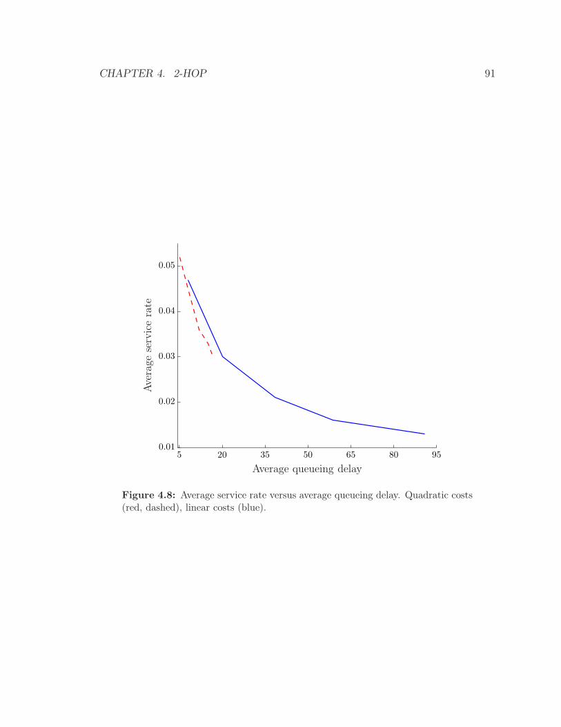
CHAPTER 4. 2-HOP 91
Ave
rage
serv
ice
rate
Average queueing delay5 20 35 50 65 80 95
0.01
0.02
0.03
0.04
0.05
Figure 4.8: Average service rate versus average queueing delay. Quadratic costs(red, dashed), linear costs (blue).
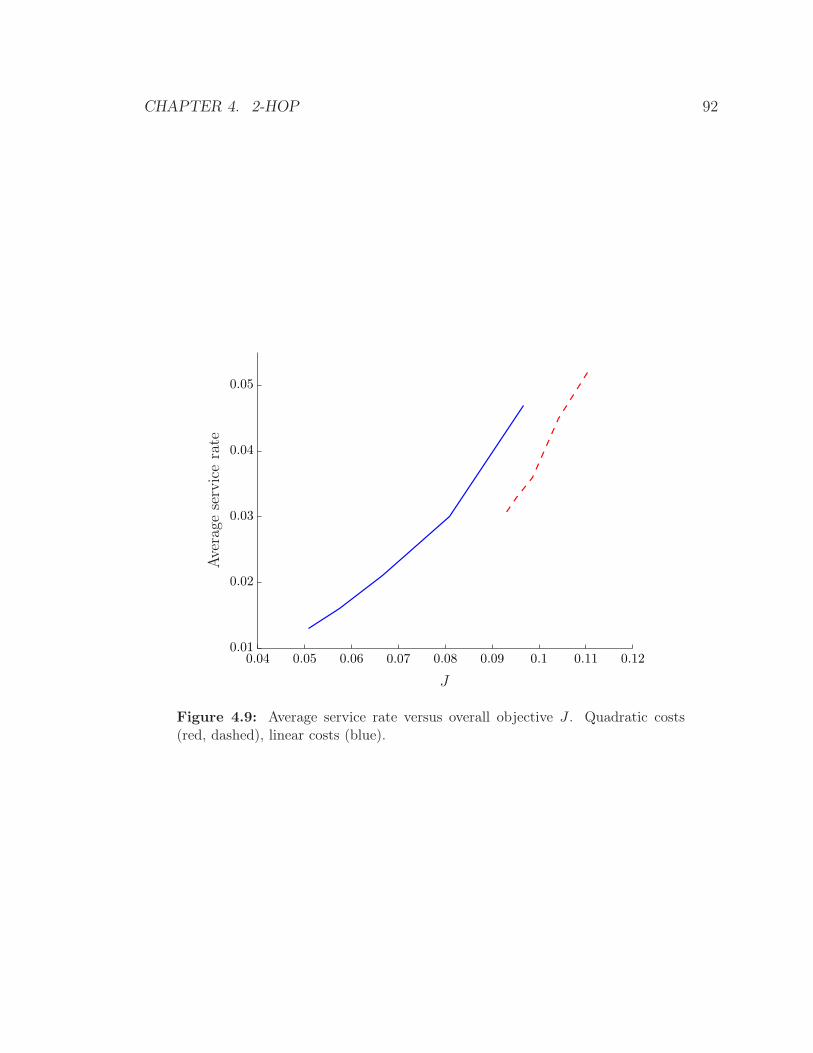
CHAPTER 4. 2-HOP 92
Ave
rage
serv
ice
rate
J
0.04 0.05 0.06 0.07 0.08 0.09 0.1 0.11 0.120.01
0.02
0.03
0.04
0.05
Figure 4.9: Average service rate versus overall objective J . Quadratic costs(red, dashed), linear costs (blue).
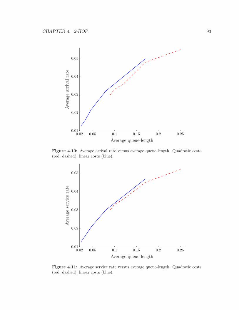
CHAPTER 4. 2-HOP 93
Ave
rage
arri
valra
te
Average queue-length0.02 0.05 0.1 0.15 0.2 0.25
0.01
0.02
0.03
0.04
0.05
Figure 4.10: Average arrival rate versus average queue-length. Quadratic costs(red, dashed), linear costs (blue).
Ave
rage
serv
ice
rate
Average queue-length0.02 0.05 0.1 0.15 0.2 0.25
0.01
0.02
0.03
0.04
0.05
Figure 4.11: Average service rate versus average queue-length. Quadratic costs(red, dashed), linear costs (blue).

CHAPTER 4. 2-HOP 94
χ(q) J sqr Q A S D
0.1q2 0.1103 0.25 0.055 0.052 5.050.25q2 0.1042 0.17 0.048 0.045 8.000.5q2 0.0986 0.12 0.036 0.036 11.900.75q2 0.0951 0.10 0.033 0.033 14.93
q2 0.0924 0.09 0.030 0.030 16.67
Table 4.4: Performance metrics for quadratic queue costs.
χ(q) J lin Q A S D
0.1q 0.0967 0.17 0.050 0.047 8.130.25q 0.0808 0.08 0.032 0.030 20.000.5q 0.0665 0.047 0.022 0.021 38.460.75q 0.0575 0.033 0.016 0.016 58.82
q 0.0509 0.024 0.013 0.013 90.91
Table 4.5: Performance metrics for linear costs.
Tables 4.4 and 4.5 summarize these metrics for quadratic and linear queue costs
respectively. We observe that Q <∞ for each of the examples, which is a necessary
condition for system stability.
4.7 Multiple flows
Similar to §3.5.1 we can construct an approximate policy for the case of multiple flows
as follows:
ϕ⋆(q, g) = argmaxF(q)
(
−m∑
i=1
φi(fi, gi) + U(fm) + V (q + Af)
)
,
where
V = V s1 + · · ·+ V s
l ,

CHAPTER 4. 2-HOP 95
is an approximate value function. Note that V sk : R → R is the optimal value function
from the associated single-hop case.
4.8 Conclusion
In this chapter we extended the flow rate control problem to the 2-link case where
we assign flow rates to optimally tradeoff average utility and average power and
queue maintenance costs. In the case of a single flow, we showed how maximum
(positive) utility and the associated average queue-length, vary with different utility
and transmit and queue cost functions. We claim that this maximal average queue-
length is a good way to size flow rate buffers depending on network traffic. We define
and derive performance metrics to distinguish single flow controllers, and give the
associated approximate controller for the case of multiple flows.
Bibliography
[AB10] E. Akuiyibo and S. Boyd. Adaptive modulation with smoothed flow
utility. EURASIP J. on Wireless Communications and Networking, 2010,
2010.
[ABFG+93] A. Arapostathis, V. Borkarand, E. Fernández-Gaucherand, M. K. Ghosh,
and S. I. Marcus. Discrete-time controlled Markov processes with aver-
age cost criterion: A survey. SIAM J. on Control and Optimization,
31(2):282–344, 1993.
[ABO10] E. Akuiyibo, S. Boyd, and D. O’Neill. Adaptive modulation in wireless
networks with smoothed flow utility. In Proceedings of IEEE Globecom,
pages 1–5, 2010.
[AM90] B. Anderson and J. Moore. Optimal Control - Linear Quadratic Methods.
Prentice-Hall, 1990.
[Åst70] K. Åström. Introduction to Stochastic Control Theory. Dover, 1970.
[AST01] M. Akian, A. Sulem, and M. Taksar. Dynamic optimization of long-term
growth rate for a portfolio with transaction costs and logarithmic utility.
Mathematical Finance, 11(2):152–188, 2001.
96
BIBLIOGRAPHY 97
[BD62] R. Bellman and S. Dreyfus. Applied Dynamic Programming. Princeton
University Press, 1962.
[Bel57] R. Bellman. Dynamic Programming. Courier Dover Publications, 1957.
[Bem06] A. Bemporad. Model predictive control design: New trends and tools.
In Proceedings of 45th IEEE Conference on Decision and Control, pages
6678–6683, 2006.
[Ber98] D. Bertsekas. A new value iteration method for the average cost dynamic
programming problem. SIAM J. on Control and Optimization, 36:742–
759, 1998.
[Ber05] D. Bertsekas. Dynamic Programming and Optimal Control: Volume 1.
Athena Scientific, 2005.
[Ber07] D. Bertsekas. Dynamic Programming and Optimal Control: Volume 2.
Athena Scientific, 2007.
[BGGN04] A. Ben-Tal, A. Goryashko, E. Guslitzer, and A. Nemirovski. Adjustable
robust solutions of uncertain linear programs. Mathematical Program-
ming, 99:351–376, 2004.
[BGW90] R. Bitmead, M. Gevers, and V. Wertz. Adaptive Optimal Control: The
Thinking Man’s GPC. Prentice-Hall, 1990.
[BK97] I. Buckley and R. Korn. Optimal Cash Management for Equity Index
Tracking in the Presence of Fixed and Proportional Transaction Costs.
Johannes-Gutenberg-Univ., 1997.
[BL97] J. Birge and F. Louveaux. Introduction to Stochastic Programming.
Springer, 1997.
BIBLIOGRAPHY 98
[BL00] J. Borwein and A. Lewis. Convex Analysis and Nonlinear Optimization.
Springer, 2000.
[Bla62] D. Blackwell. Discrete dynamic programming. Ann. Math. Statist.,
33:719–726, 1962.
[BN98] A. Ben-Tal and A. Nemirovski. Robust convex optimization. Mathemat-
ics of Operations Research, 23(4):769–805, 1998.
[BN07] A. Ben-Tal and A. Nemirovski. Selected topics in robust convex opti-
mization. Mathematical Programming: Series A and B, 112(1):125–158,
2007.
[BNO03] D. Bertsekas, A. Nedić, and A. Ozdaglar. Convex Analysis and Opti-
mization. Athena Scientific, 2003.
[BS96] D. Bertsekas and S. Shreve. Stochastic optimal control: The discrete-time
case. Athena Scientific, 1996.
[BSS10] D. Brown, J. Smith, and P. Sun. Information relaxations and duality in
stochastic dynamic programs. Operations Research, 2010. To appear.
[BT96] D. Bertsekas and J. Tsitsiklis. Neuro-Dynamic Programming. Athena
Scientific, 1996.
[BTN01] A. Ben-Tal and A. Nemirovski. Lectures on Modern Convex Optimiza-
tion. Analysis, Algorithms, and Engineering Applications. Society for
Industrial and Applied Mathematics, 2001.
[BV04] S. Boyd and L. Vandenberghe. Convex Optimization. Cambridge Uni-
versity Press, 2004.
BIBLIOGRAPHY 99
[Cav72] J. Cavers. Variable-rate transmission for Rayleigh fading channels. IEEE
Transactions on Communication Technology, 20(1):15–22, 1972.
[CC05a] G. Calafiore and M. Campi. On two-stage portfolio allocation problems
with affine recourse. In Proceedings of the 44th IEEE Conference on
Decision and Control, and the European Control Conference 2005, pages
8042–8047, 2005.
[CC05b] G. Calafiore and M. Campi. Uncertain convex programs: Randomized
solutions and confidence levels. Mathematical Programming, 102(1):25–
46, 2005.
[CD07] G. Calafiore and F. Dabbene. Probabilistic robust control. In Proceeding
of the 2007 American Control Conference, pages 147–158, 2007.
[CGH+96] R. Corless, G. Gonnet, D. Hare, D. Jeffrey, and D. Knuth. On the
Lambert W function. Advances in Computational Mathematics, 5:329–
359, 1996.
[CK96] J. Cvitanić and I. Karatzas. Hedging and portfolio optimization under
transaction costs: A martingale approach. Mathematical Finance, 6:133–
166, 1996.
[CL88] M. Corless and G. Leitmann. Controller design for uncertain system via
Lyapunov functions. In Proceedings of the American Control Conference,
volume 3, pages 2019–2025, 1988.
[Cla95] K. Clarkson. Las vegas algorithms for linear and integer programming
when the dimension is small. J. ACM, 42(2):25–46, 1995.
[CLCD07] M. Chiang, S. Low, A. Calderbank, and J. Doyle. Distributed rate allo-
cation for inelastic flows. Proceedings of the IEEE, 95:255–312, 2007.
BIBLIOGRAPHY 100
[Con79] G. Constantinides. Multiperiod consumption and investment behavior
with convex transaction costs. Management Science, 25:1127–1137, 1979.
[CS05] M. Casey and S. Sen. The scenario generation algorithm for multistage
stochastic linear programming. Mathematics of Operations Research,
30(3):615–631, 2005.
[Cut83] C. Cutler. Dynamic Matrix Control: An Optimal Mutlivariable Control
Algorithm with Constraints. PhD thesis, University of Houston, 1983.
[CXH+10] J. Chen, W. Xu, S. He, Y. Sun, P. Thulasiraman, and X. Shen. Utility-
based asynchronous flow control algorithm for wireless sensor networks.
IEEE Journal on Selected Areas in Communications, 28(7):1116–1126,
2010.
[DDB95] M. Dahleh and I. Diaz-Bobillo. Control of Uncertain Systems: A Linear
Programming approach. Prentice-Hall, 1995.
[Dem95] R. Dembo. Optimal portfolio replication. Algorithmics Technical paper
series, 9501, 1995.
[Den82] E. Denardo. Dynamic Programming: Models and Applications. Prentice-
Hall, 1982.
[Der66] C. Derman. Denumerable state Markov decision processes — average
cost criterion. Ann. Math. Statist., 37:1545–1553, 1966.
[Der70] C. Derman. Finite state Markovian decision processes. Academic Press,
1970.
[dFR03] D. de Farias and B. Van Roy. The linear programming approach to
approximate dynamic programming. Operations Research, 51(6):850–
865, 2003.
BIBLIOGRAPHY 101
[dFR04] D. de Farias and B. Van Roy. On constraint sampling in the linear pro-
gramming approach to approximate dynamic programming. Operations
Research, 29(3):462–478, 2004.
[DI93] G. Dantzig and G. Infanger. Multi-stage stochastic linear programs for
portfolio optimization. Annals of Operations Research, 45:59–76, 1993.
[DL81] C. Desoer and R. Liu. Global parametrization of feedback systems. Deci-
sion and Control including the Symposium on Adaptive Processes, 1981
20th IEEE Conference on, 20:859–861, 1981.
[DL91] B. Dumas and E. Luciano. An exact solution to a dynamic portfo-
lio choice problem under transaction costs. The Journal of Finance,
46(2):577–595, 1991.
[DN90] M. Davis and A. Norman. Portfolio selection with transaction costs.
Mathematics of Operations Research, 15(4):676–713, 1990.
[DP00] G. Dullerud and F. Paganini. A Course in Robust Control Theory: a
Convex Approach. Springer-Verlag, New York, 2000.
[DR00] R. Dembo and D. Rosen. The practice of portfolio replication. Algo
Research Quarterly, 3(2):11–22, 2000.
[ED98] N. Elia and M. Dahleh. Computational Methods for Controller Design.
Springer-Verlag, 1998.
[ES07] A. Eryilmaz and R. Srikant. Fair resource allocation in wireless networks
using queue-length-based scheduling and congestion control. IEEE/ACM
Transactions on Networking, 15(6):1333–1344, 2007.
BIBLIOGRAPHY 102
[EW88] Y. Ermoliev and R. Wets. Numerical Techniques for stochastic optimiza-
tion. Springer-Verlag, 1988.
[FP96] R. Freeman and J. Primbs. Control Lyapunov functions: New ideas from
an old source. In Proceedings of the 35th IEEE Conference on Decision
and Control, pages 3926–3931, Kobe, Japan, 1996.
[FPEN94] G. Franklin, J. Powell, and A. Emami-Naeini. Feedback Control of Dy-
namic Systems. Addison-Wesley, 1994.
[FPW80] G. Franklin, J. Powell, and M. Workman. Digital Control of Dynamic
Systems. Addison-Wesley, 1980.
[FvdS09] F. Fu and M. van der Schaar. A systematic framework for dynamically
optimizing multi-user wireless video transmission. Technical report, Me-
dia Lab, University of California, Los Angeles, 2009.
[GBY06] M. Grant, S. Boyd, and Y. Ye. CVX: Matlab software for disci-
plined convex programming, 2006. Available at http://www. stanford.
edu/ boyd/cvx.
[GC97] A. Goldsmith and S. Chua. Variable rate variable power MQAM for
fading channels. IEEE Transactions on Communications, 45(10):1218–
1230, 1997.
[GC98] A. Goldsmith and S. Chua. Adaptive coded modulation for fading chan-
nels. IEEE Transactions on Communications, 46(5):595–602, 1998.
[GK07] P. Goulart and E. Kerrigan. Output feedback receding horizon control of
constrained systems. International Journal of Control, 80(1):8–20, 2007.
BIBLIOGRAPHY 103
[GK08] P. Goulart and E. Kerrigan. Input-to-state stability of robust receding
horizon control with an expected value cost. Automatica, 44(4):1171–
1174, 2008.
[GKM06] P. Goulart, E. Kerrigan, and J. Maciejowski. Optimization over state
feedback policies for robust control with constraints. Automatica,
42(4):523–533, 2006.
[GNT06] L. Georgiadis, M. Neely, and L. Tassiulas. Resource allocation and cross-
layer control in wireless networks. Foundations and Trends in Network-
ing, 1(1):1–144, 2006.
[Hay68] J. Hayes. Adaptive feedback communications. IEEE Transactions on
Communication Technology, 16(1):29–34, 1968.
[HBVL97] A. Hansson, S. Boyd, L. Vandenberghe, and M. Lobo.
Optimal linear static control with moment and yield
objectives. Unpublished manuscript. Available at
http://www.stanford.edu/~boyd/papers/yield.html, 1997.
[Hen74] V. Hentinen. Error performance for adaptive transmission on fad-
ing channels. IEEE Transactions on Communication Technology,
22(9):1331–1337, 1974.
[HLCK08] J. Huang, Z. Li, M. Chiang, and A. Katsaggelos. Joint source adaptation
and resource allocation for multi-user wireless video streaming. IEEE
Transactions on Circuits and Systems for Video Technology, 18(5):582–
595, 2008.
BIBLIOGRAPHY 104
[HWL00] D. Goodman H. Wang, N. Mandayam and P. Ligdas. Dynamic utility
maximization for mobile data communications under delay constraints.
In Proceedings of IEEE VTC, 2000.
[JCOB02] D. Julian, M. Chiang, D. O’Neill, and S. Boyd. Qos and fairness con-
strained convex optimization of resource allocation for wireless cellular
and ad hoc networks. In Proceedings of INFOCOM, pages 477–486, 2002.
[KH05] W. Kwon and S. Han. Receding Horizon Control. Springer-Verlag, 2005.
[KM05] P. Kall and J. Mayer. Stochastic Linear Programming: Models, Theory,
and Computation. Springer, 2005.
[KMT97] F. Kelly, A. Maulloo, and D. Tan. Rate control for communication net-
works: Shadow prices, proportional fairness and stability. Journal of the
Operational Research Society, 49:237–252, 1997.
[KV86] P. Kumar and P. Varaiya. Stochastic systems: Estimation, identification
and adaptive control. Prentice-Hall, 1986.
[KW04] H. Kusher and P. Whiting. Convergence of proportional-fair sharing
algorithms under general conditions. IEEE Transactions on Wireless
Communications, 3(4):1250–1259, 2004.
[L03a] J. Löfberg. Approximations of closed-loop minimax MPC. In Proceedings
of 42nd IEEE Conference on Decision and Control, 2003., volume 2,
pages 1438–1442, 2003.
[L03b] J. Löfberg. Minimax approaches to robust model predictive control. PhD
thesis, Linköping University, 2003.
BIBLIOGRAPHY 105
[LFB07] M. Lobo, M. Fazel, and S. Boyd. Portfolio optimization with linear and
fixed transaction costs. Annals of Operations Research, 152(1):376–394,
2007.
[Liu05] H. Liu. Optimal consumption and investment with transaction costs and
multiple risky assets. The Journal of Finance, 59(1):289–338, 2005.
[LL99] S. Low and D. Lapsley. Optimization flow control I: Basic algorithms
and convergence. IEEE/ACM Transactions on Networking, 7(6):861–
874, 1999.
[LL02] H. Liu and M. Loewenstein. Optimal portfolio selection with transaction
costs and finite horizons. Review of Financial Studies, 15(3):805–835,
2002.
[Loa78] C. Van Loan. Nineteen dubious ways to compute the matrix exponential.
SIAM Review, 20(4):801–836, 1978.
[LR07] X. Lin and S. Rasool. A distributed joint channel-assignment, scheduling
and routing algorithm for multi-channel ad hoc wireless networks. In
Proceedings of the IEEE Infocom, Anchorage, 2007.
[Man60] A. Manne. Linear programming and sequential decisions. Management
Science, 6(3):259–267, 1960.
[Mar03] P. Martí Colom. Analysis and Design of Realtime Control Systems with
Varying Control Timing Constraints. PhD thesis, Universitat Politècnica
de Catalunya, June 2003.
[MB08] J. Mattingley and S. Boyd. CVXMOD - Convex optimization software
in python, 2008. Available at http://cvxmod.net.
BIBLIOGRAPHY 106
[MBL10] R. Madan, S. Boyd, and S. Lall. Fast algorithms for resource allocation
in wireless cellular networks. IEEE Transactions on Networking, 2010.
To appear.
[MC76] M. Magill and G. Constantinides. Portfolio selection with transaction
costs. J. Econ. Theory, 13:245–263, 1976.
[Mey06] S. Meyn. Control Techniques for Complex Networks. Cambridge Univer-
sity Press, 2006.
[MRRS00] D. Q. Mayne, J. B. Rawlings, C. V. Rao, and P. O. M. Scokaert. Con-
strained model predictive control: Stability and optimality. Automatica,
36(6):789–814, June 2000.
[NBW98] J. Nilsson, B. Bernhardsson, and B. Wittenmark. Some topics in real-
time control. In Proceedings of the American Control Conference, vol-
ume 4, pages 2386–2390, 1998.
[NML08] M. Neely, E. Modiano, and C. Li. Fairness and optimal stochastic control
for heterogeneous networks. IEEE/ACM Transactions on Networking,
16(2):396–409, 2008.
[NMR05] M. Neely, E. Modiano, and C. Rohrs. Dynamic power allocation and
routing for time-varying wireless networks. IEEE/JSAC, 23(1):89–103,
2005.
[OABG10] D. O’Neill, E. Akuiyibo, S. Boyd, and A. Goldsmith. Optimizing adap-
tive modulation in wireless networks via multi-period network utility
maximization. In Proceedings of International Conference on Communi-
cations, 2010.

BIBLIOGRAPHY 107
[OGB08a] D. O’Neill, A. Goldsmith, and S. Boyd. Cross-layer design with adaptive
modulation: Delay, rate, energy tradeoffs. In Proceedings of Globecom,
2008.
[OGB08b] D. O’Neill, A. Goldsmith, and S. Boyd. Optimizing adaptive modu-
lation in wireless networks via utility maximization. In Proceedings of
International Conference on Communications, 2008.
[PC06] D. Palomar and M. Chiang. Alternative decompositions for distributed
maximization of network utility: framework and applications. In Pro-
ceedings of the IEEE Infocom, Barcelona, 2006.
[Pow07] W. Powell. Approximate dynamic programming: Solving the curses of
dimensionality. John Wiley & Sons, 2007.
[PPR04] S. Prajna, P. Parrilo, and A. Rantzer. Nonlinear control synthesis by con-
vex optimization. IEEE Transactions on Automatic Control, 49(2):310–
314, 2004.
[PPSV+02] L. Palopoli, C. Pinello, A. Sangiovani-Vincentelli, L. El Ghaoui, and
A. Bicchi. Synthesis of robust control systems under resource constraints.
In Hybrid Systems: Computation and Control (HSCC 2002), pages 337–
350, 2002.
[Pre95] A. Prekopa. Stochastic Programming. Kluwer Academic Publishers,
1995.
[Pri07a] J. Primbs. Dynamic hedging of basket options under proportional trans-
action costs using receding horizon control. Submitted, 2007.
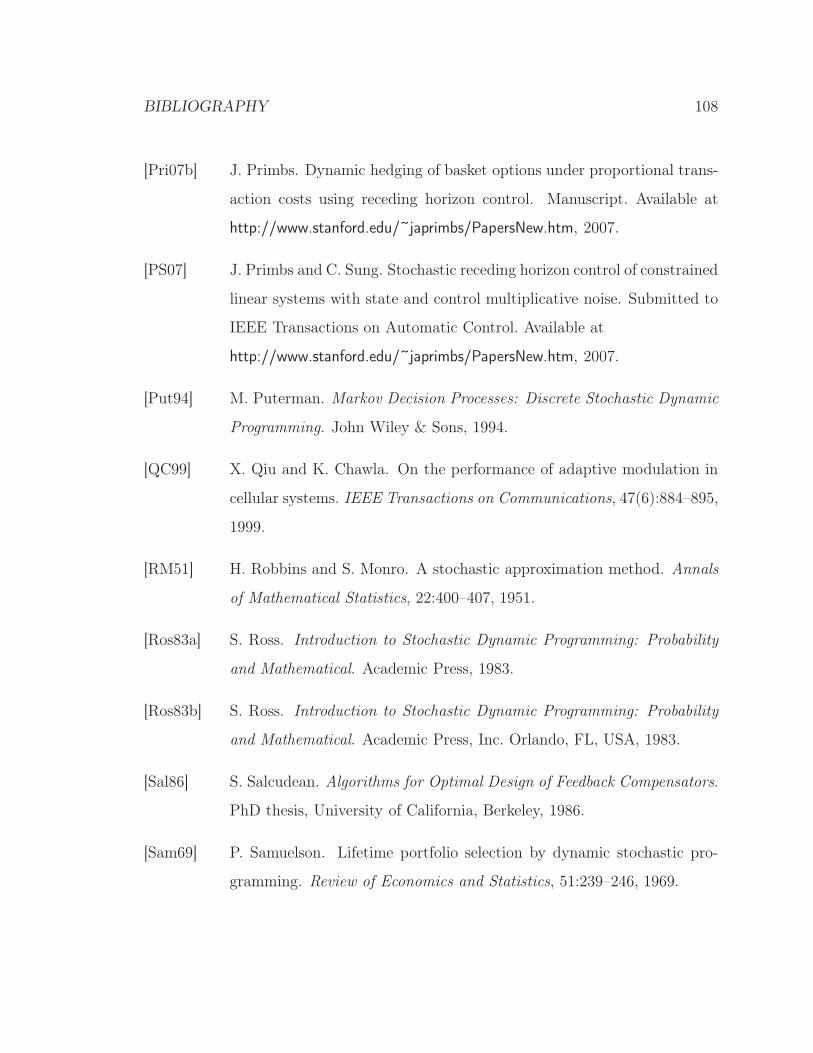
BIBLIOGRAPHY 108
[Pri07b] J. Primbs. Dynamic hedging of basket options under proportional trans-
action costs using receding horizon control. Manuscript. Available at
http://www.stanford.edu/~japrimbs/PapersNew.htm, 2007.
[PS07] J. Primbs and C. Sung. Stochastic receding horizon control of constrained
linear systems with state and control multiplicative noise. Submitted to
IEEE Transactions on Automatic Control. Available at
http://www.stanford.edu/~japrimbs/PapersNew.htm, 2007.
[Put94] M. Puterman. Markov Decision Processes: Discrete Stochastic Dynamic
Programming. John Wiley & Sons, 1994.
[QC99] X. Qiu and K. Chawla. On the performance of adaptive modulation in
cellular systems. IEEE Transactions on Communications, 47(6):884–895,
1999.
[RM51] H. Robbins and S. Monro. A stochastic approximation method. Annals
of Mathematical Statistics, 22:400–407, 1951.
[Ros83a] S. Ross. Introduction to Stochastic Dynamic Programming: Probability
and Mathematical. Academic Press, 1983.
[Ros83b] S. Ross. Introduction to Stochastic Dynamic Programming: Probability
and Mathematical. Academic Press, Inc. Orlando, FL, USA, 1983.
[Sal86] S. Salcudean. Algorithms for Optimal Design of Feedback Compensators.
PhD thesis, University of California, Berkeley, 1986.
[Sam69] P. Samuelson. Lifetime portfolio selection by dynamic stochastic pro-
gramming. Review of Economics and Statistics, 51:239–246, 1969.
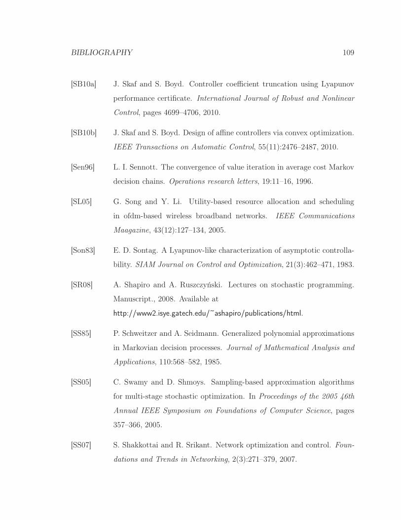
BIBLIOGRAPHY 109
[SB10a] J. Skaf and S. Boyd. Controller coefficient truncation using Lyapunov
performance certificate. International Journal of Robust and Nonlinear
Control, pages 4699–4706, 2010.
[SB10b] J. Skaf and S. Boyd. Design of affine controllers via convex optimization.
IEEE Transactions on Automatic Control, 55(11):2476–2487, 2010.
[Sen96] L. I. Sennott. The convergence of value iteration in average cost Markov
decision chains. Operations research letters, 19:11–16, 1996.
[SL05] G. Song and Y. Li. Utility-based resource allocation and scheduling
in ofdm-based wireless broadband networks. IEEE Communications
Maagazine, 43(12):127–134, 2005.
[Son83] E. D. Sontag. A Lyapunov-like characterization of asymptotic controlla-
bility. SIAM Journal on Control and Optimization, 21(3):462–471, 1983.
[SR08] A. Shapiro and A. Ruszczyński. Lectures on stochastic programming.
Manuscript., 2008. Available at
http://www2.isye.gatech.edu/~ashapiro/publications/html.
[SS85] P. Schweitzer and A. Seidmann. Generalized polynomial approximations
in Markovian decision processes. Journal of Mathematical Analysis and
Applications, 110:568–582, 1985.
[SS05] C. Swamy and D. Shmoys. Sampling-based approximation algorithms
for multi-stage stochastic optimization. In Proceedings of the 2005 46th
Annual IEEE Symposium on Foundations of Computer Science, pages
357–366, 2005.
[SS07] S. Shakkottai and R. Srikant. Network optimization and control. Foun-
dations and Trends in Networking, 2(3):271–379, 2007.
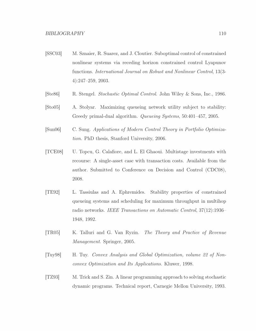
BIBLIOGRAPHY 110
[SSC03] M. Sznaier, R. Suarez, and J. Cloutier. Suboptimal control of constrained
nonlinear systems via receding horizon constrained control Lyapunov
functions. International Journal on Robust and Nonlinear Control, 13(3-
4):247–259, 2003.
[Ste86] R. Stengel. Stochastic Optimal Control. John Wiley & Sons, Inc., 1986.
[Sto05] A. Stolyar. Maximizing queueing network utility subject to stability:
Greedy primal-dual algorithm. Queueing Systems, 50:401–457, 2005.
[Sun06] C. Sung. Applications of Modern Control Theory in Portfolio Optimiza-
tion. PhD thesis, Stanford University, 2006.
[TCE08] U. Topcu, G. Calafiore, and L. El Ghaoui. Multistage investments with
recourse: A single-asset case with transaction costs. Available from the
author. Submitted to Conference on Decision and Control (CDC08),
2008.
[TE92] L. Tassiulas and A. Ephremides. Stability properties of constrained
queueing systems and scheduling for maximum throughput in multihop
radio networks. IEEE Transactions on Automatic Control, 37(12):1936–
1948, 1992.
[TR05] K. Talluri and G. Van Ryzin. The Theory and Practice of Revenue
Management. Springer, 2005.
[Tuy98] H. Tuy. Convex Analysis and Global Optimization, volume 22 of Non-
convex Optimization and Its Applications. Kluwer, 1998.
[TZ93] M. Trick and S. Zin. A linear programming approach to solving stochastic
dynamic programs. Technical report, Carnegie Mellon University, 1993.
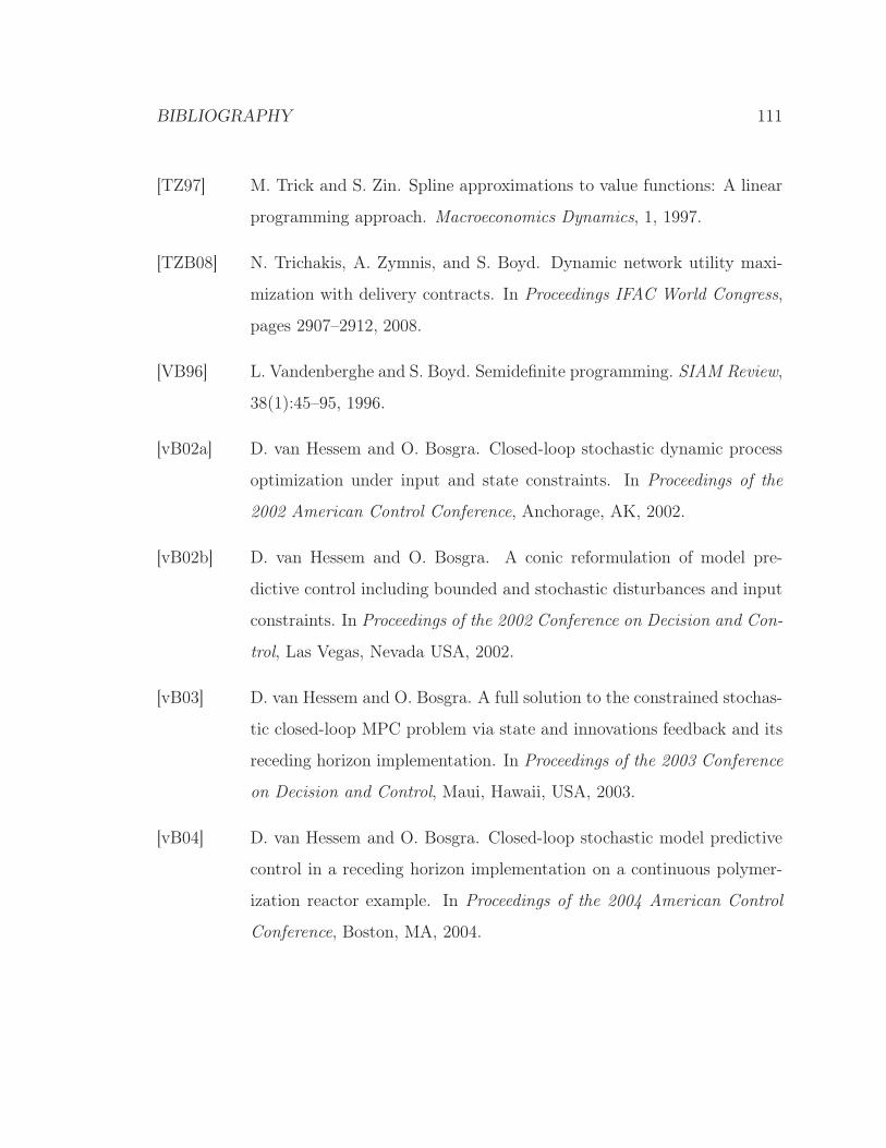
BIBLIOGRAPHY 111
[TZ97] M. Trick and S. Zin. Spline approximations to value functions: A linear
programming approach. Macroeconomics Dynamics, 1, 1997.
[TZB08] N. Trichakis, A. Zymnis, and S. Boyd. Dynamic network utility maxi-
mization with delivery contracts. In Proceedings IFAC World Congress,
pages 2907–2912, 2008.
[VB96] L. Vandenberghe and S. Boyd. Semidefinite programming. SIAM Review,
38(1):45–95, 1996.
[vB02a] D. van Hessem and O. Bosgra. Closed-loop stochastic dynamic process
optimization under input and state constraints. In Proceedings of the
2002 American Control Conference, Anchorage, AK, 2002.
[vB02b] D. van Hessem and O. Bosgra. A conic reformulation of model pre-
dictive control including bounded and stochastic disturbances and input
constraints. In Proceedings of the 2002 Conference on Decision and Con-
trol, Las Vegas, Nevada USA, 2002.
[vB03] D. van Hessem and O. Bosgra. A full solution to the constrained stochas-
tic closed-loop MPC problem via state and innovations feedback and its
receding horizon implementation. In Proceedings of the 2003 Conference
on Decision and Control, Maui, Hawaii, USA, 2003.
[vB04] D. van Hessem and O. Bosgra. Closed-loop stochastic model predictive
control in a receding horizon implementation on a continuous polymer-
ization reactor example. In Proceedings of the 2004 American Control
Conference, Boston, MA, 2004.
BIBLIOGRAPHY 112
[VBW98] L. Vandenberghe, S. Boyd, and S. Wu. Determinant maximization with
linear matrix inequality constraints. SIAM Journal on Matrix Analysis
and Applications, 19(2):499–533, 1998.
[Vid85] M. Vidyasagar. Control System Synthesis: A Factorization Approach.
MIT press, 1985.
[VM10] G. Vejarna and J. McNair. Queue-stability-based transmission power
control in wireless multihop networks. In Proceedings of Globecom, 2010.
[VW69] R. Van Slyke and R. Wets. L-shaped linear programs with applications
to optimal control and stochastic linear programming. SIAM Journal of
Applied Mathematics, 17:638–663, 1969.
[WB08] Y. Wang and S. Boyd. Fast model predictive control using online opti-
mization. In Proceedings IFAC World Congress, pages 6974–6997, July
2008.
[WB09] Y. Wang and S. Boyd. Performance bounds for linear stochastic control.
Systems and Control Letters, 58(3):178–182, 2009.
[Whi82] P. Whittle. Optimization Over Time: Dynamic Programming and
Stochastic Control. Wiley, 1982.
[WNT95] B. Wittenmark, J. Nilsson, and M. Torngren. Timing problems in real-
time control systems. In Proceedings of the American Control Confer-
ence, volume 3, pages 2000–2004, 1995.
[WOS07] C. Wang, C. Ong, and M. Sim. Model predictive control using affine dis-
turbance feedback for constrained linear system. 46th IEEE Conference
on Decision and Control, 2007, pages 1275–1280, 2007.
BIBLIOGRAPHY 113
[WS95] W. Webb and R. Steele. Variable rate QAM for mobile radio. IEEE
Transactions on Communications, 43(7):2223–2230, 1995.
[WSW99] B. Wah, Y. Shang, and Z. Wu. Discrete Lagrangian methods for opti-
mizing the design of multiplierless QMF banks. IEEE Transactions on
Circuits and Systems II, 46(9):1179–1191, 1999.
[YBJ76] D. Youla, J. Bongiorno, and H. Jabr. Modern Wiener-Hopf design of
optimal controllers–Part I: The single-input-output case. IEEE Trans-
actions on Automatic Control, 21:3–13, 1976.
[YJB76] D. Youla, H. Jabr, and J. Bongiorno. Modern Wiener-Hopf design of
optimal controllers–Part II: The multivariable case. IEEE Transactions
on Automatic Control, 21:319–338, 1976.
[ZDG96] K. Zhou, J. Doyle, and K. Glover. Robust and Optimal Control. Prentice-
Hall, 1996.
[ZTN08] X. Zhan, M. Tao, and C. Ng. Utility-based wireless resource allocation
for variable rate transmission. IEEE Transactions on Wireless Commu-
nications, 7(9):3292–3296, 2008.
[ZV06] W. Ziemba and R. Vickson. Stochastic Optimization Models in Finance.
World Scientific, 2006.