dwh – dimesional modeling pdt genči. 2 outline requirement gathering fact and dimension table...
TRANSCRIPT
DWH – Dimesional Modeling
PDT
Genči
2
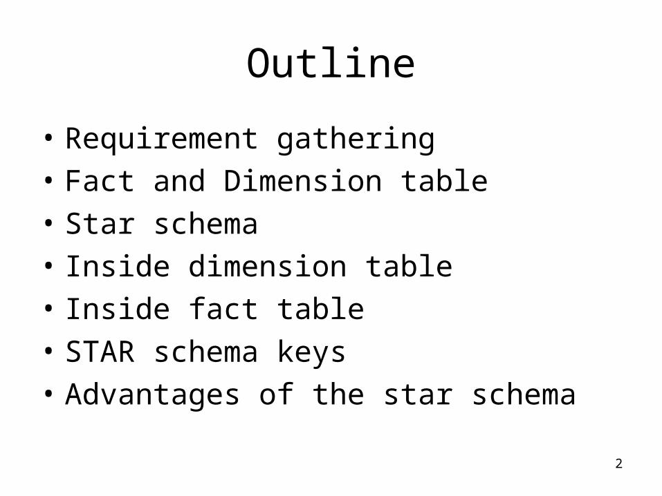
Outline
• Requirement gathering
• Fact and Dimension table
• Star schema
• Inside dimension table
• Inside fact table
• STAR schema keys
• Advantages of the star schema
3
4
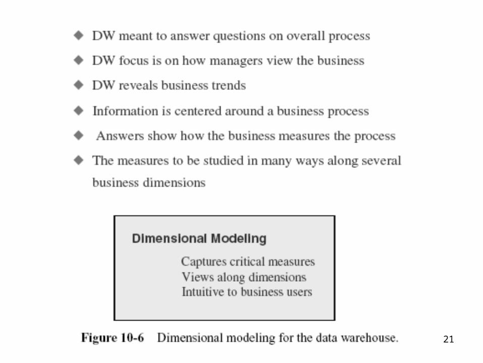
Dimensional Modeling Basics
• Dimensional modeling gets its name from the business dimensions we need to incorporate into the logical data model.
• It is a logical design technique to structure the business dimensions and the metrics that are analyzed along these dimensions.
• This modeling technique is intuitive for that purpose.
• The model has also proved to provide high performance for queries and analysis.
5
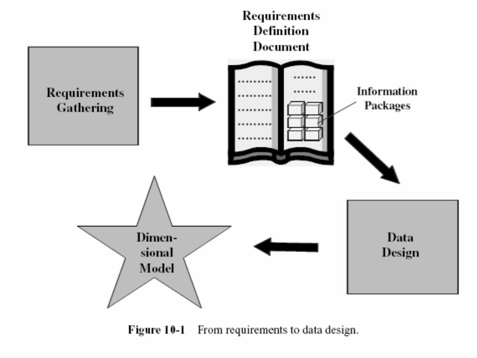
Requirements gathering
• The traditional methods applicable to operational systems are not adequate in DWH.
• We cannot start with the functions, screens, and reports.
• We cannot begin with the data structures. • Users tend to think in terms of business
dimensions and analyze measurements along such business dimensions.
• This is a significant observation and can form the very basis for gathering information
6
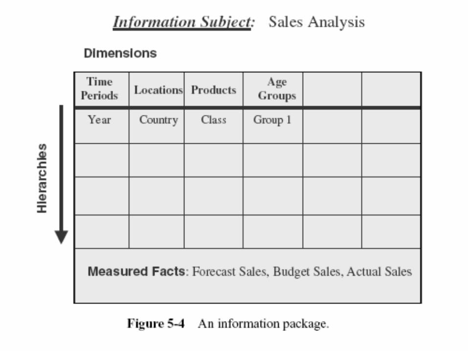
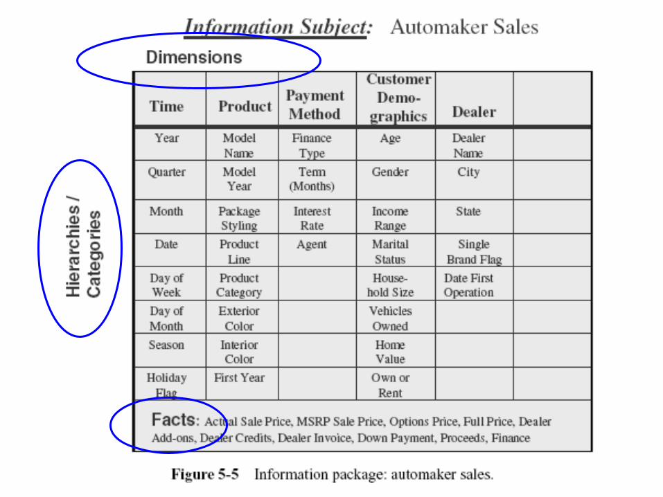
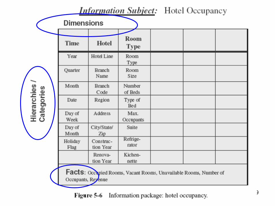
INFORMATION PACKAGES
• Methodology for requirements gathering
7
8
9
10
How the fact table is formed
• The fact table gets its name from the subject for analysis.
• Each fact item or measurement goes into the fact table as an attribute
11
12
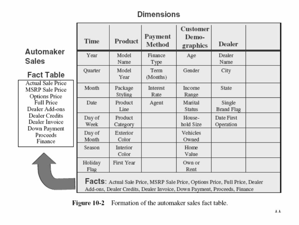
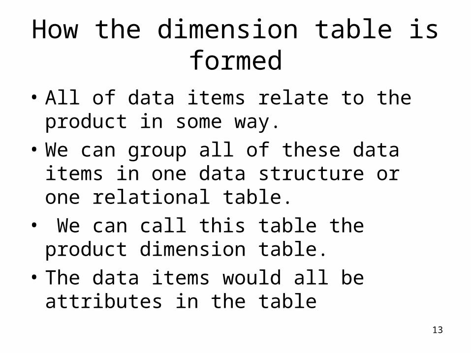
How the dimension table is formed
• The product business dimension is used when we want to analyze the facts by products
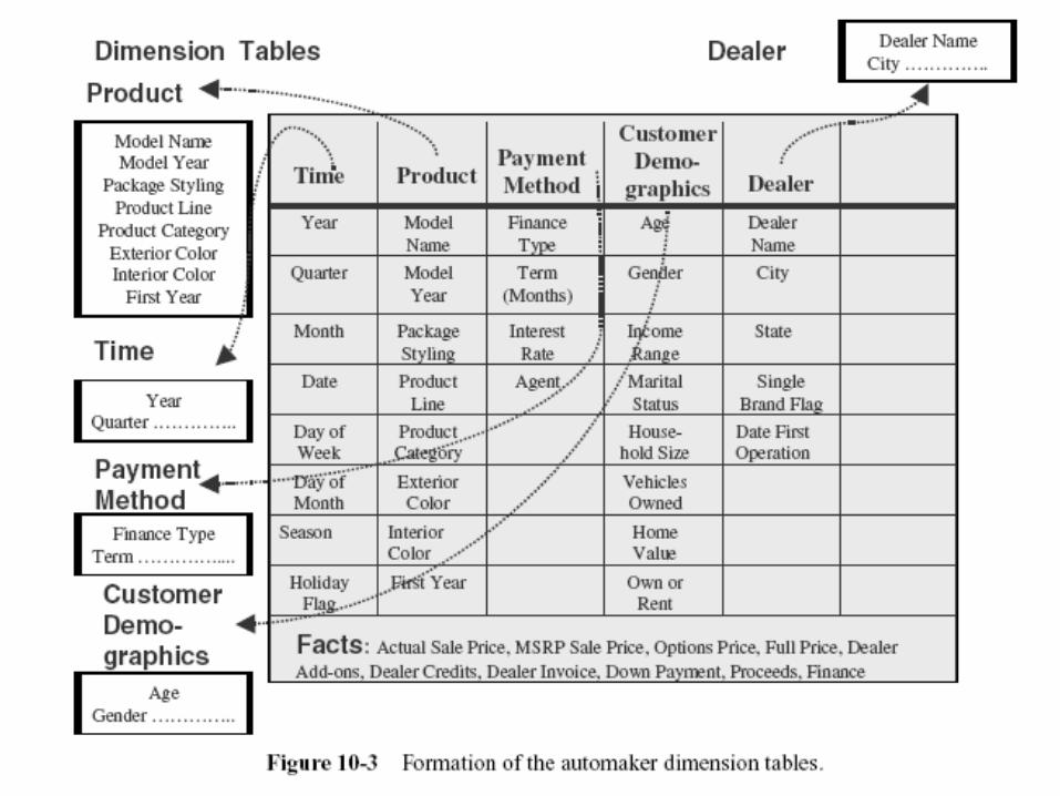
• The list of data items relating to the product dimension are as follows:
• Model name• Model year• Package styling• Product line• Product category• Exterior color• Interior color• First model year
13
How the dimension table is formed
• All of data items relate to the product in some way.
• We can group all of these data items in one data structure or one relational table.
• We can call this table the product dimension table.
• The data items would all be attributes in the table
14
15
• We have formed the fact table and the dimension tables.
• How should these tables be arranged in the dimensional model?
16
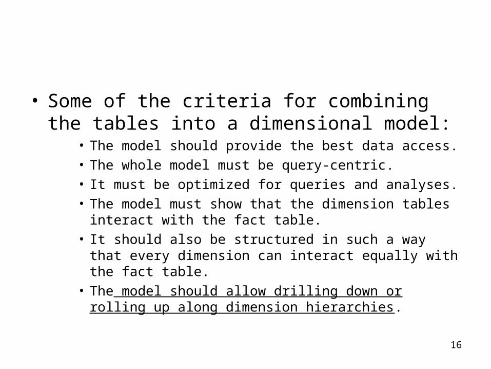
• Some of the criteria for combining the tables into a dimensional model:
• The model should provide the best data access.• The whole model must be query-centric.• It must be optimized for queries and analyses.• The model must show that the dimension tables interact with
the fact table.• It should also be structured in such a way that every
dimension can interact equally with the fact table.• The model should allow drilling down or rolling up along
dimension hierarchies.
17
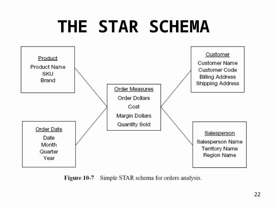
• With these requirements, we find that a dimensional model with the fact table in the middle and the dimension tables arranged around the fact table satisfies the conditions.
• In this arrangement, each of the dimension tables has a direct relationship with the fact table in the middle.
• This is necessary because every dimension table with its attributes must have an even chance of participating in a query to analyze the attributes in the fact table
18
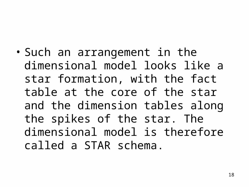
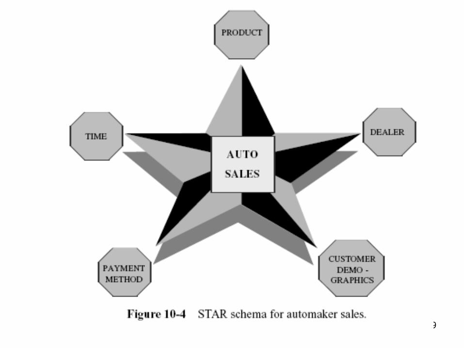
• Such an arrangement in the dimensional model looks like a star formation, with the fact table at the core of the star and the dimension tables along the spikes of the star. The dimensional model is therefore called a STAR schema.
19
20
21
22
THE STAR SCHEMA
23
Example
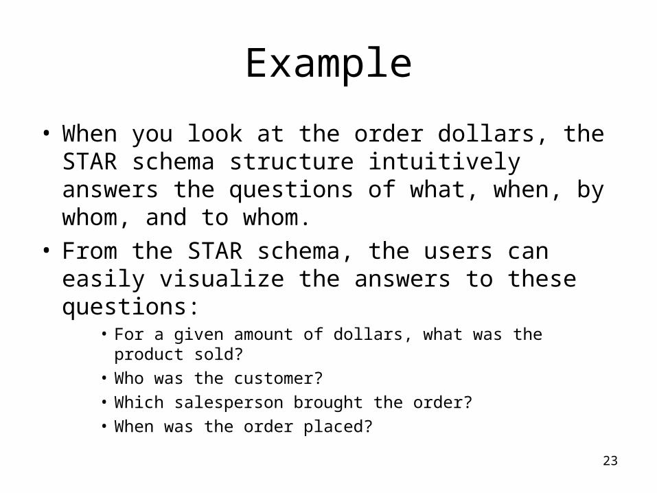
• When you look at the order dollars, the STAR schema structure intuitively answers the questions of what, when, by whom, and to whom.
• From the STAR schema, the users can easily visualize the answers to these questions:
• For a given amount of dollars, what was the product sold? • Who was the customer? • Which salesperson brought the order? • When was the order placed?
24
• The STAR schema structure is a structure that can be easily understood by the users and with which they can comfortably work.
• The structure mirrors how the users normally view their critical measures along their business dimensions.
25
• When a query is made against the data warehouse, the results of the query are produced by combining or joining one of more dimension tables with the fact table.
• The joins are between the fact table and individual dimension tables.
• The relationship of a particular row in the fact table is with the rows in each dimension table. These individual relationships are clearly shown as the spikes of the STAR schema.
26
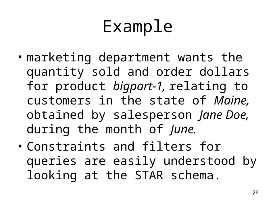
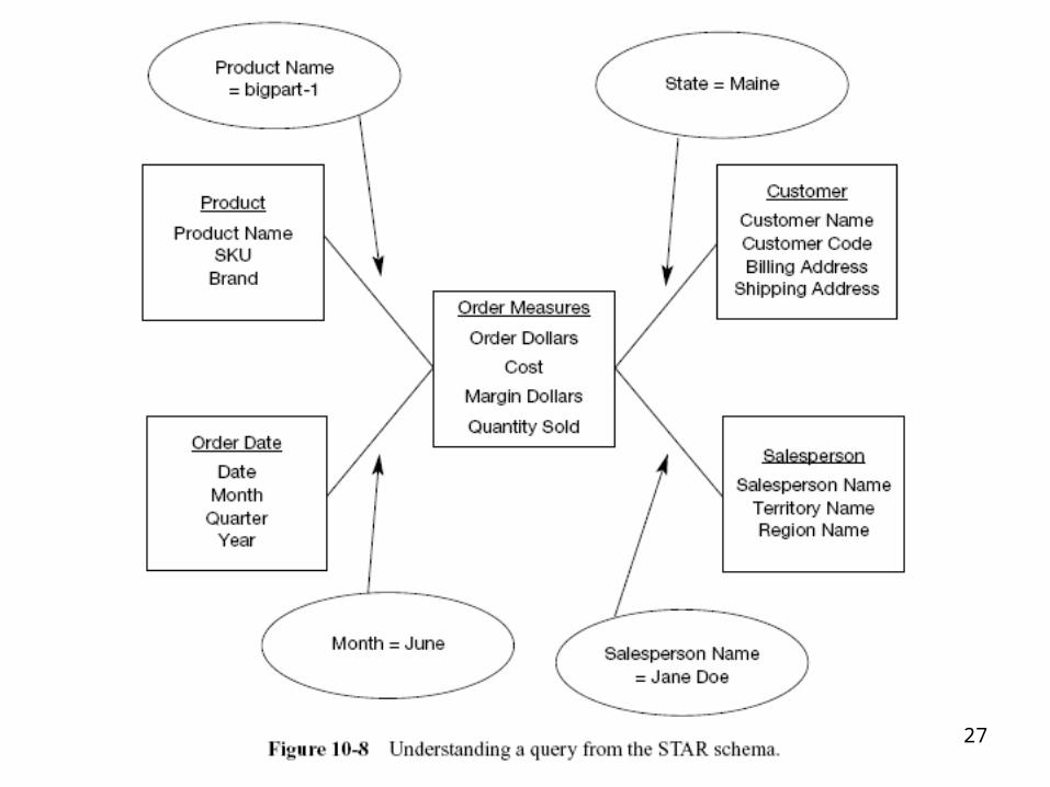
Example
• marketing department wants the quantity sold and order dollars for product bigpart-1, relating to customers in the state of Maine, obtained by salesperson Jane Doe, during the month of June.
• Constraints and filters for queries are easily understood by looking at the STAR schema.
27
28
Drill down
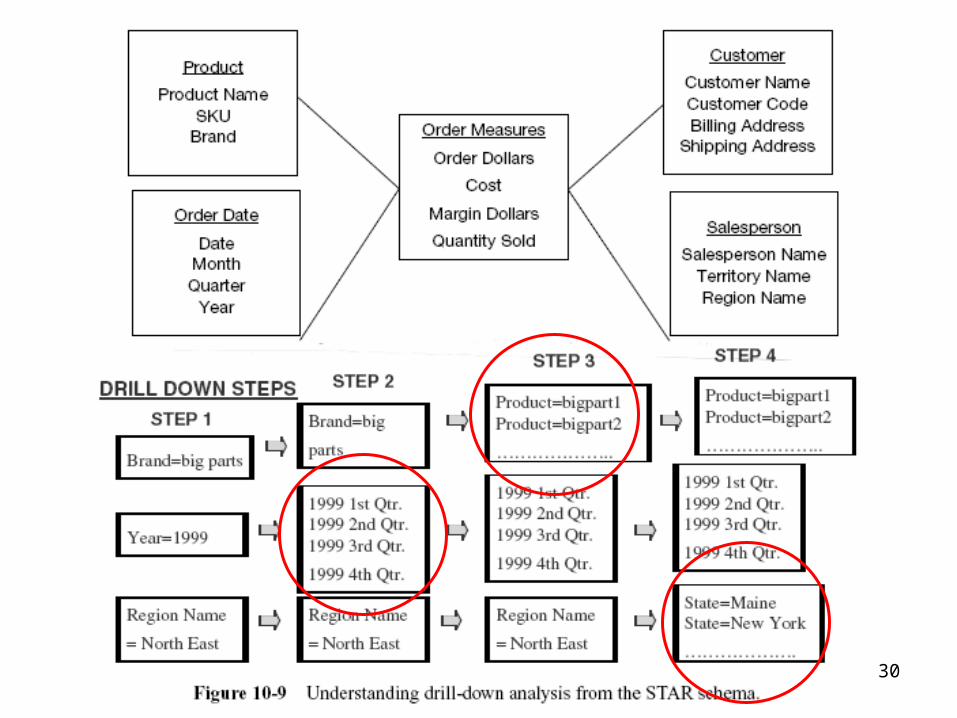
• A common type of analysis is the drilling down of summary numbers to get at the details at the lower levels.
29
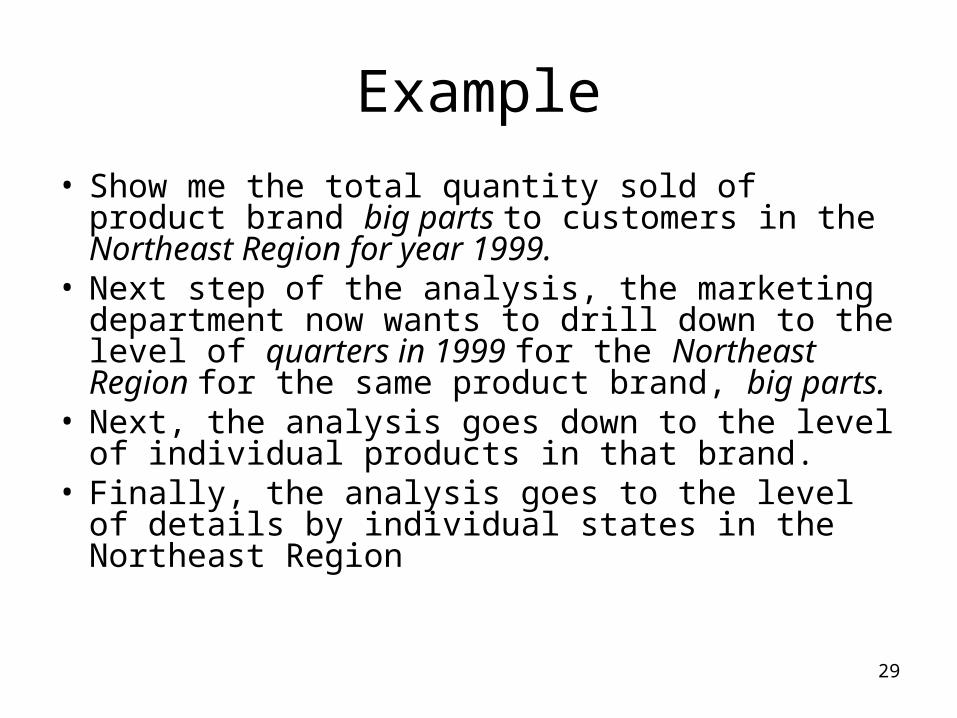
Example
• Show me the total quantity sold of product brand big parts to customers in the Northeast Region for year 1999.
• Next step of the analysis, the marketing department now wants to drill down to the level of quarters in 1999 for the Northeast Region for the same product brand, big parts.
• Next, the analysis goes down to the level of individual products in that brand.
• Finally, the analysis goes to the level of details by individual states in the Northeast Region
30
Inside a Dimension Table
32
Inside a Dimension Table
• We have seen that a key component of the STAR schema is the set of dimension tables.
• The dimension tables represent the business dimensions along which the metrics are analyzed.
• We look inside a dimension table and study its characteristics.
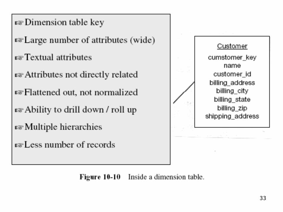
33
34
Dimension table key
• Primary key of the dimension table uniquely identifies each row in the table.
35
Table is wide
Typically, a dimension table has many columns or attributes.
It is not uncommon for some dimension tables to have more than fifty attributes - we say that the dimension table is wide.
If you lay it out as a table with columns and rows, the table is spread out horizontally.
36
Textual attributes
• In the dimension table you will seldom find any numerical values used for calculations.
• The attributes in a dimension table are of textual format.
• These attributes represent the textual descriptions of the components within the business dimensions.
• Users will compose their queries using these descriptors.
37
Attributes not directly related
Frequently you will find that some of the attributes in a dimension table are not directly related to the other attributes in the table.
For example, package size is not directly related to product brand; nevertheless, package size and product brand could both be attributes of the product dimension table.
38
Not normalized
• The attributes in a dimension table are used in queries. • An attribute is taken as a constraint in a query and
applied directly to the metrics in the fact table. • For efficient query performance, it is best if the query
picks up an attribute from the dimension table and goes directly to the fact table and not through other intermediary tables.
• If you normalize the dimension table, you will be creating such intermediary tables and that will not be efficient.
• Therefore, a dimension table is flattened out, not normalized.
39
Drilling down, rolling up
• The attributes in a dimension table provide the ability to get to the details from higher levels of aggregation to lower levels of details.
• For example, the three attributes zip, city, and state form a hierarchy. You may get the total sales by state, then drill down to total sales by city, and then by zip. Going the other way, you may first get the totals by zip, and then roll up to totals by city and state
40
Multiple hierarchies
• Dimension tables often provide for multiple hierarchies, so that drilling down may be performed along any of the multiple hierarchies
• Example (product dimension table for a department store):
• marketing–product–category, • marketing–product–department, • finance–product–category, • finance–product–department
41
Fewer number of records
• A dimension table typically has fewer number of records or rows than the fact table.
• A product dimension table for an automaker may have just 500 rows.
Inside the Fact Table
43
Inside the Fact Table
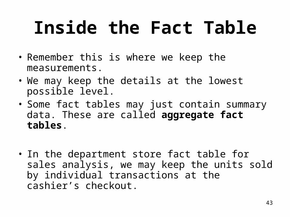
• Remember this is where we keep the measurements.
• We may keep the details at the lowest possible level.
• Some fact tables may just contain summary data. These are called aggregate fact tables.
• In the department store fact table for sales analysis, we may keep the units sold by individual transactions at the cashier’s checkout.
44
45
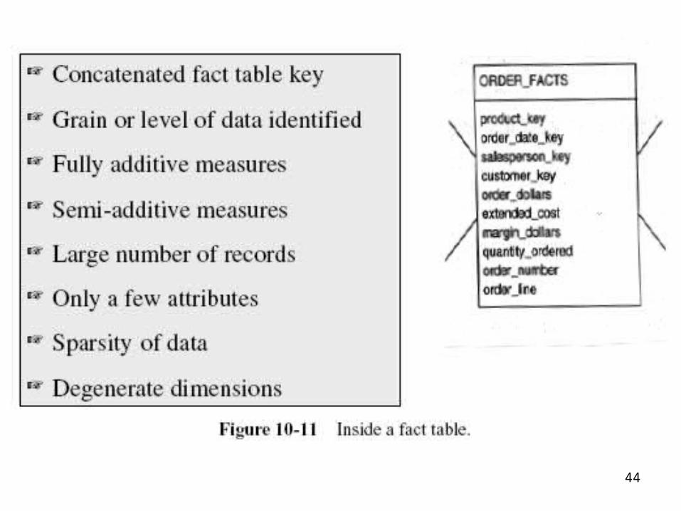
Concatenated Key
• A row in the fact table relates to a combination of rows from all the dimension tables.
• Example:• the dimension tables are product, time, customer, and
sales representative. • For these dimension tables, assume that the lowest level in
the dimension hierarchies are individual product, a calendar date, a specific customer, and a single sales representative.
• Then a single row in the fact table must relate to a particular product, a specific calendar date, a specific customer, and an individual sales representative.
• This means the row in the fact table must be identified by the primary keys of these four dimension tables.
• Thus, the primary key of the fact table must be the concatenation of the primary keys of all the dimension tables.
46
Data Grain
• The data grain is the level of detail for the measurements or metrics
• Example:• The metrics are at the detailed level. • The quantity ordered relates to the quantity of a
particular product on a single order, on a certain date, for a specific customer, and procured by a specific sales representative.
• If we keep the quantity ordered as the quantity of a specific product for each month, then the data grain is different and is at a higher level.
47
Fully Additive Measures
The values of these attributes may be summed up by simple addition.
Such measures are known as fully additive measures. Aggregation of fully additive measures is done by simple
addition. When we run queries to aggregate measures in the fact
table, we will have to make sure that these measures are fully additive.
Otherwise, the aggregated numbers may not show the correct totals.
• order_dollars, extended_cost, and quantity_ordered
48
Semiadditive Measures
Derived attributes may not be additive. They are known as semiadditive
measures. Distinguish semiadditive measures from
fully additive measures when you perform aggregations in queries.
order_dollars is 120 and extended_cost is 100, the margin_percentage is 20
49
Table Deep, Not Wide
Typically a fact table contains fewer attributes than a dimension table.
Usually, there are about 10 attributes or less. But the number of records in a fact table is very large. If you lay the fact table out as a two-dimensional table,
you will note that the fact table is narrow with a small number of columns, but very deep with a large number of rows.
Example: Take a very simplistic example of 3 products, 5 customers, 30 days,
and 10 sales representatives represented as rows in the dimension tables. Even in this example, the number of fact table rows will be 4500, very large in comparison with the dimension table rows.
50
Sparse Data
• single row in the fact table relates to a particular product, a specific calendar date, a specific customer, and an individual sales representative
• In other words, for a particular product, a specific calendar date, a specific customer, and an individual sales representative, there is a corresponding row in the fact table.
• What happens when the date represents a closed holiday and no orders are received and processed?
• The fact table rows for such dates will not have values for the measures.
51
Sparse Data
• there could be other combinations of dimension table attributes, values for which the fact table rows will have null measures.
• There is no need to keep rows with null measures in the fact table.
• It is important to realize this type of sparse data and understand that the fact table could have gaps.
52
Degenerate Dimensions
• When you pick up attributes for the dimension tables and the fact tables from operational systems, you will be left with some data elements in the operational systems that are neither facts nor strictly dimension attributes.
• These attributes are useful in some types of analyses.
• Such attributes are called degenerate dimensions and these are kept as attributes of the fact table
53
The Factless Fact Table
• Apart from the concatenated primary key, a fact table contains facts or measures
• In the situation when the fact table represents events, fact tables do not need to contain facts
• Such tablea are called “factless” fact tables
54
Data Granularity
• Granularity represents the level of detail in the fact table
• When you keep the fact table at the lowest grain, the users could drill down to the lowest level of detail from the data warehouse without the need to go to the operational systems themselves
• Base level fact tables must be at the natural lowest levels of all corresponding dimensions
• Queries for drill-down and roll-up can be performed efficiently
55
Data Granularity (2)
• We have to pay the price in terms of storage and maintenance for the fact table at the lowest grain.
• Lowest grain necessarily means large numbers of fact table rows.
• In practice, however, we build aggregate fact tables to support queries looking for summary numbers.
56
Advantages of granular fact tables
• Fact tables at the lowest grain facilitate “graceful” extensions
• Granular fact tables serve as natural destinations for current operational data that may be extracted frequently from operational systems.
• The more recent data mining applications need details at the lowest grain
STAR SCHEMA KEYS
58
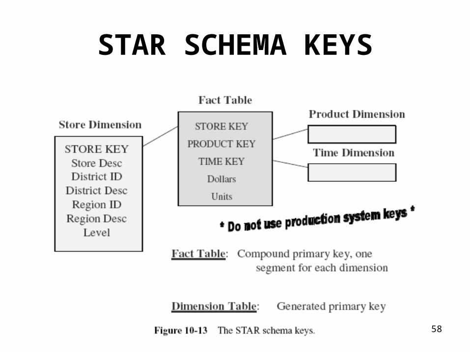
STAR SCHEMA KEYS
59
Primary Keys
• Avoid built-in meanings in the primary key of the dimension tables
• Do not use production system keys as primary keys for dimension tables
• Use surrogate keys
60
Surrogate keys
• The surrogate keys are simply system-generated sequence numbers.
• They do not have any built-in meanings.
• Surrogate keys will be mapped to the production system keys.
• The general practice is to keep the operational system keys as additional attributes in the dimension tables.
61
Foreign Keys
• Each dimension table is in a one-to-many relationship with the central fact table.
• So the primary key of each dimension table must be a foreign key in the fact table.
• If there are four dimension tables of product, date, customer, and sales representative, then the primary key of each of these four tables must be present in the orders fact table as foreign keys.
62
Primary keys for the fact tables 1. A single compound primary key whose length is the total length of the
keys of the individual dimension tables. Under this option, in addition to the compound primary key, the foreign keys must also be kept in the fact table as additional attributes. This option increases the size of the fact table.
2. Concatenated primary key that is the concatenation of all the primary keys of the dimension tables. Here you need not keep the primary keys of the dimension tables as additional attributes to serve as foreign keys. The individual parts of the primary keys themselves will serve as the foreign keys.
3. A generated primary key independent of the keys of the dimension tables. In addition to the generated primary key, the foreign keys must also be kept in the fact table as additional attributes. This option also increases the size of the fact table.
• In practice, option (2) is used in most fact tables. This option enables you to easily relate the fact table rows with the dimension table rows.
63
ADVANTAGES OF THE STAR SCHEMA
• Although the STAR schema is a relational model, it is not a normalized model.
• The dimension tables are purposely denormalized.
• This is a basic difference between the STAR schema and relational schemas for OLTP systems
64
ADVANTAGES OF THE STAR SCHEMA (2)
• Easy for Users to Understand
• Optimizes Navigation
• Most Suitable for Query Processing including to drill down or roll up
• STARjoin and STARindex