UNIVERSITY OF JYVASKYLADEPARTMENT OF MATHEMATICS

AND STATISTICS

REPORT 130

UNIVERSITAT JYVASKYLAINSTITUT FUR MATHEMATIK

UND STATISTIK

BERICHT 130

EXISTENCE AND UNIQUENESS OFp(x)-HARMONIC FUNCTIONS FORBOUNDED AND UNBOUNDED p(x)

JUKKA KEISALA

JYVASKYLA2011

UNIVERSITY OF JYVASKYLADEPARTMENT OF MATHEMATICS

AND STATISTICS

REPORT 130

UNIVERSITAT JYVASKYLAINSTITUT FUR MATHEMATIK

UND STATISTIK

BERICHT 130

EXISTENCE AND UNIQUENESS OFp(x)-HARMONIC FUNCTIONS FORBOUNDED AND UNBOUNDED p(x)

JUKKA KEISALA

JYVASKYLA2011

Editor: Pekka KoskelaDepartment of Mathematics and StatisticsP.O. Box 35 (MaD)FI–40014 University of JyvaskylaFinland

ISBN 978-951-39-4299-1ISSN 1457-8905

Copyright c© 2011, Jukka Keisalaand University of Jyvaskyla

University Printing HouseJyvaskyla 2011

Contents

0 Introduction 30.1 Notation and prerequisities . . . . . . . . . . . . . . . . . . . . . 6

1 Constant p, 1 < p <∞ 81.1 The direct method of calculus of variations . . . . . . . . . . . . 101.2 Dirichlet energy integral . . . . . . . . . . . . . . . . . . . . . . . 10

2 Infinity harmonic functions, p ≡ ∞ 132.1 Existence of solutions . . . . . . . . . . . . . . . . . . . . . . . . 142.2 Uniqueness of solutions . . . . . . . . . . . . . . . . . . . . . . . 182.3 Minimizing property and related topics . . . . . . . . . . . . . . . 22

3 Variable p(x), with 1 < inf p(x) < sup p(x) < +∞ 24

4 Variable p(x) with p(·) ≡ +∞ in a subdomain 304.1 Approximate solutions uk . . . . . . . . . . . . . . . . . . . . . . 324.2 Passing to the limit . . . . . . . . . . . . . . . . . . . . . . . . . . 39

5 One-dimensional case, where p is continuous and sup p(x) = +∞ 455.1 Discussion . . . . . . . . . . . . . . . . . . . . . . . . . . . . . . . 455.2 Preliminary results . . . . . . . . . . . . . . . . . . . . . . . . . . 475.3 Measure of p(x) = +∞ is positive . . . . . . . . . . . . . . . . 48

6 Appendix 51

References 55

0 Introduction

In this licentiate thesis we study the Dirichlet boundary value problem−∆p(x)u(x) = 0, if x ∈ Ω,

u(x) = f(x), if x ∈ ∂Ω.(0.1)

Here Ω ⊂ Rn is a bounded domain, p : Ω → (1,∞] a measurable function,f : ∂Ω → R the boundary data, and −∆p(x)u(x) is the p(x)-Laplace operator,which is written as

−∆p(x)u(x) = −div(|∇u(x)|p(x)−2∇u(x)

)for finite p(x). If p(·) ≡ p for 1 < p <∞, then the p(x)-Laplace operator reducesto the standard p-Laplace operator

−∆pu(x) = −div(|∇u(x)|p−2∇u(x)

).

For p(x) =∞ we consider the infinity Laplace operator,

−∆∞u(x) = −n∑

i,j=1

∂u

∂xi(x)

∂u

∂xj(x)

∂2u

∂xi∂xj(x), (0.2)

which is formally derived from the p-Laplace equation −∆pu = 0 by sendingp to infinity. We study the problem (0.1) in different cases, depending on thefunction p, and our aim is to show that this problem has a unique solution ineach of these cases. The merit of this work is in that it is the first survey of theknown existence and uniqueness results for (0.1), although not complete, sincethe borderline cases p = 1 and inf p(x) = 1 are outside the scope of this work.

We consider five different cases, all with different assumptions on p(x), andall of them have been distributed into their own sections. The theory is pre-sented in chronological order thus following how the research on the p(x)-Laplaceoperator has advanced.

The first case is the most well-known case where p is a constant function,1 < p < ∞. The p-harmonic functions (i.e., the solutions of the p-Laplaceequation −∆pu = 0) have been widely studied during the past sixty years. Bystudying p-harmonic functions one learns a lot about different fields of mathe-matics, such as calculus of variations and partial differential equations, and it isa good model case for more general nonlinear elliptic equations. The theory ofp-harmonic functions is quite well developed, albeit there are some well-knownopen problems left, see, e.g., the survey [24]. In the first section we presentthe direct method of calculus of variations to find a function u that is a uniqueminimizer to the Dirichlet energy integral

I(v) :=

∫Ω

|∇v(x)|p dx

I would like to thank Professor Petri Juutinen for introducing me to the theory of p(x)-harmonic functions and for many valuable discussions and advice. I also want to thankProfessor Julio D. Rossi and Docent Petteri Harjulehto for reviewing this thesis and for theirvaluable comments. For financial support I am indebted to the University of Jyvaskyla andto the Vilho, Yrjo and Kalle Vaisala Foundation.

3

in the set v ∈W 1,p(Ω) : v−f ∈W 1,p0 (Ω). Then we show that there is a one to

one correspondence between the minimizer of the energy integral and problem(0.1), i.e., u is a minimizer of the integral if and only if u solves (0.1). The samemethod will be used in Sections 3 and 4.

In the second case we study infinity harmonic functions (i.e., the solutionsof the infinity Laplace equation −∆∞u = 0). The articles by Gunnar Aronsson([4], [5] and a handful of others) in the 1960s were the start-up point in this field.Aronsson started by studying the optimal Lipschitz extensions and found theconnection between them and infinity harmonic functions. At that time viscositysolutions had not yet been discovered and the expression (0.2) could be verifiedonly for C2-functions. Later, in the 1980s, the concept of viscosity solutions waspresented and it gave a new view to examine the infinity harmonic functions.Using p-harmonic approximation, it was easy to prove that the problem (0.1)has a solution, but the uniqueness was harder to prove. Jensen proved thatfirst in 1993 in his paper [21]. In 2001, Crandall, Evans and Gariepy usedviscosity solutions to prove the connection that Aronsson found, see [9]. Thisis presented in Theorem 2.15. In 2009, Armstrong and Smart [3] found a new,easy way to prove the uniqueness. The research of infinity harmonic functions isquite intensive today. Especially, the regularity of infinity harmonic functions isstill an unsolved problem in dimensions three or higher. The infinity harmonicequation also works as a model case for more general Aronsson-Euler equations.We recommend the survey [6] by Aronsson, Crandall and Juutinen to get awider picture of infinity harmonic functions and related problems.

In the third section we assume that the function p is non-constant andbounded, and 1 < inf p(x) < sup p(x) < ∞. The research of variable expo-nent Lebesgue and Sobolev spaces started in 1991, when the seminal paper byKovacik and Rakosnık [23] was published. They defined spaces Lp(·) and W k,p(·)

and proved the basic properties of these spaces. Although the Lp(·)-functionsshare many properties with standard Lp-functions, they, in general, lack a so-called p(x)-mean continuity property. Because of this, the convolution of anLp(·)-function and a C∞0 -function does not belong to Lp(·) in general. Then thestandard convolution approximation, which is familiar from the Lp-spaces, can-not be generalized to variable exponent Lebesgue spaces, and hence the densityof smooth functions in Lp(·) becomes an untrivial issue. However, by addingsome extra conditions on p(x), from which the log-Holder continuity

|p(x)− p(y)| ≤ C

log(e+ 1/|x− y|)

is the most important, this problem can be avoided and the density problemsolved, see [12] and [26]. The log-Holder continuity is also a sufficient conditionon p(x) so that the variable exponent Sobolev-Poincare inequality holds. Thisinequality is crucial when proving the existence of the solution of (0.1). Aftersolving these difficulties, the variable p(x)-case becomes practically identicalwith the constant p-case from the standpoint of the problem (0.1). The researchof variable exponent spaces is a growing field in nonlinear analysis nowadays,and there are still many open problems left and waiting to be solved. To get acomprehensive view of variable exponent Lebesgue and Sobolev spaces, we askthe reader to get acquainted with a book by Diening, Harjulehto, Hasto andRuzicka [11].

4

In the fourth case we assume that p(x) ≡ ∞ in a subdomain D of Ω, andthat p|Ω\D is C1-smooth and bounded. This case is based on the article [25] byManfredi, Rossi and Urbano. Their article was the first attempt to analyze theproblem (0.1) when the variable exponent is not bounded. The approach to thiscase is the following: first find a unique solution uk to the problem (0.1) withpk(x) = mink, p(x) by using the direct method of calculus of variations, thenget estimates for uk and ∇uk that are independent of k, after that pass to thelimit k →∞ to get a limit function u∞ and find out what equation it solves.

In the final, fifth, case we consider a one-dimensional case where p is contin-uous and unbounded on the interval (a, b) with limx→b− p(x) =∞, and infinityon (b, c); here a < b < c. The unboundedness of p on (a, b) causes differentproblems that we discuss. In view of these problems it is easy to see why theboundedness assumption for p|Ω\D was made in the fourth section. Our analysiswill not be very deep, and we shall only draw some guidelines. The generaliza-tions of our results to higher dimensions is an interesting open problem.

Next we shall say something about the cases that have been left out of thiswork. In the case p = 1 the (standard) p-Laplace operator is

−∆1u(x) = − div

(∇u(x)

|∇u(x)

).

In the associated variational problem we should try to find a unique minimizerfor the functional I, where

I(v) :=

∫Ω

|∇v(x)| dx,

in the set v ∈ W 1,1(Ω) : v − f ∈ W 1,10 (Ω). The first problem now is that

W 1,1(Ω) is not reflexive and I is not strictly convex, and thus the direct methodof calculus of variations is no more applicable. The corresponding problemcan be formulated in BV (Ω) (the class of functions u ∈ L1(Ω) whose partialderivatives in the sense of distributions are measures with finite total variationin Ω) as follows: for f ∈ C(∂Ω), find a minimizer for ‖∇v‖(Ω) in the set v ∈BV (Ω) ∩ C(Ω), u = f on ∂Ω. Here

‖∇v‖(Ω) = sup

∫Ω

v div σ dx : σ ∈ C∞0 (Ω;Rn), |σ(x)| ≤ 1 for x ∈ Ω

.

If Ω is a Lipschitz domain, then it is quite easy to construct the minimizer forthis problem in the space BV (Ω), but the question that the minimizer is contin-uous and satisfies the boundary condition, is more subtle. The behaviour of ∂Ωplays an essential role in this question. By assuming that ∂Ω has non-negativemean curvature in a weak sense and that ∂Ω is not locally area-minimizing, thecontinuity and the boundary condition of the minimizer can be verified. Onthe other hand, if neither condition on ∂Ω is true, then it is possible to con-struct a boundary data f such that the corresponding problem has no solution.The uniqueness of solutions can also be obtained under the aforementioned as-sumptions on ∂Ω. Since the nature of this problem is quite different from thecases we treat, we do not consider it any further in this work. See [27] for adetailed study of this case and [22], where the minimizers of the above problemare approximated by p-harmonic functions as p→ 1. See also [18], in which the

5

authors consider the minimization problem related to (0.1) in the case wherethe variable exponent p : Ω→ [1,∞) attains the value 1.

The regularity of solutions of (0.1) is beyond the scope of this thesis. If thereader is interested in regularity, we recommend the following articles/surveys:[24] for p-harmonic functions, [1], [2] and [7] for variable p(x)-harmonic func-tions, and [13] and [14] for infinity harmonic functions.

0.1 Notation and prerequisities

We shall use the following notation throughout this thesis. For a set A in theeuclidean space Rn, ∂A is its boundary and A is its closure. The notationA ⊂⊂ B means that A is an open subset of B whose closure A is a compactsubset of B. The euclidean distance between two sets, A and B, is denoted bydist (A,B), and dist (x,A) is the distance from x to A. The diameter of A isdiam (A).

Throughout this work we shall assume that Ω ⊂ Rn is a bounded domain(=open and connected) with n ≥ 2, except in Section 5 where Ω is an openinterval in R. The Lebesgue measure of a measurable set A is denoted by |A|.The open ball with center at x ∈ Rn and radius r > 0 is B(x, r) = y ∈ Rn :|x − y| < r. The boundary of the ball, y ∈ Rn : |x − y| = r, is denoted by∂B(x, r) or, equivalently, by S(x, r).

The class of continuous functions in A is denoted by C(A). For an open setA, the class Ck(A) consists of all k times continuously differentiable functions u :A→ R. When we say that u : A→ R is a classical solution (or smooth solution)to some equation, we mean that u is at least twice continuously differentiable,and when we talk about the density of smooth functions, we mean by the wordsmooth that the functions are infinitely many times continuously differentiable,that is, they are members of the class C∞(A). By Ck0 (A) we denote all thefunctions u ∈ Ck(A), for which the support of u, sptu, is a compact subset of A.A function u ∈ Ck(A) belongs to class Ck,α(A), if all k-th order derivatives ofu are Holder continuous with exponent 0 < α < 1. For a Lipschitz continuousfunction f : A→ R we denote the Lipschitz constant of f by

Lip (f,A) = sup

|f(x)− f(y)||x− y|

: x, y ∈ A, x 6= y

.

Let A be a measurable set and 1 ≤ p ≤ ∞. We define a Lebesgue spaceLp(A) by

Lp(A) := u : A→ R is measurable : ‖u‖Lp(A) < +∞,

where the Lp-norm of u is

‖u‖Lp(A) :=

(∫A

|u(x)|p dx) 1

p

,

for 1 ≤ p <∞ and‖u‖L∞(A) := ess sup

x∈A|u(x)|

for p = ∞. Then Lp(A) is Banach space. The space Lploc(A) consists of allmeasurable functions u for which u ∈ Lp(K) for every compact K ⊂ A. If

6

p ∈ (1,∞), then the dual space of Lp(A) is Lq(A), where 1/p + 1/q = 1, andthe space Lp(A) is reflexive.

For an open set B, the Sobolev space W 1,p(B) consists of functions u ∈Lp(B), whose weak gradient ∇u belongs to Lp(B). The space W 1,p(B) is Ba-nach space with the norm

‖u‖W 1,p(B) := ‖u‖Lp(B) + ‖∇u‖Lp(B).

The local space W 1,ploc (B) is defined in the same way as the local Lp-space, and

the Sobolev space with zero boundary values, W 1,p0 (B), is defined as the closure

of C∞0 (B) with respect to the Sobolev norm ‖·‖W 1,p(B). For p ∈ (1,∞), thespace W 1,p(B) is reflexive and the dual space is W 1,q(B); here 1/p+ 1/q = 1.

We present the inequalities that will be used frequently. The Holder inequal-ity ∫

A

|f(x)g(x)| dx ≤ ‖f‖Lp(A)‖g‖Lq(A)

holds for f ∈ Lp(A) and g ∈ Lq(A), where 1/p+1/q = 1. The Sobolev inequality

‖∇u‖Lp(B) ≤ C(n, p,B)‖∇u‖Lp(B)

is true if B is an open set with finite measure, u ∈W 1,p0 (B) and 1 < p <∞. If

n < p <∞ and u ∈W 1,p(Rn), then Morrey’s inequality

|u(x)− u(y)| ≤ C(n, p)|x− y|1−np ‖∇u‖Lp(Rn)

holds for every x, y ∈ R. For the proofs of the inequalities above and for moreinformation concerning Lebesgue and Sobolev spaces, we ask reader to see [16]and [29].

We assume that the reader of this work knows the basics from functionalanalysis and from measure and integration theory. Also the knowledge on calcu-lus of variations and on partial differential equations helps the reader to followthe text. For example, the book by Giusti [16] is of great help and gives morethan sufficient prerequisities.

7

1 Constant p, 1 < p <∞In this section, we consider the case where the function p is constant, 1 < p <∞.Then the Dirichlet boundary value problem is written as

−∆pu(x) = 0, if x ∈ Ω,

u(x) = f(x), if x ∈ ∂Ω.(1.1)

Here f : ∂Ω→ R is the boundary data and

−∆pu(x) = −div(|∇u(x)|p−2∇u(x)

)= −|∇u(x)|p−4

|∇u(x)|2∆u(x) + (p− 2)

n∑i,j=1

uxi(x)uxj

(x)uxixj(x)

is the p-Laplace operator. Our aim is to show that the problem (1.1) has aunique solution.

Since the class of classical solutions (i.e., C2-functions for which−∆pu(x) = 0and u(x) = f(x) could be verified pointwise) is too small to treat the problem(1.1) properly, we need to use the concept of weak solutions. Then the boundaryvalues are determined by the function f ∈W 1,p(Ω). The fact that an arbitraryfunction u is a weak solution to the problem (1.1) means two things:

1) u is a weak solution of the equation −∆pu = 0 in Ω.

2) u equals f on ∂Ω in the Sobolev sense, that is, u− f ∈W 1,p0 (Ω).

The concept of weak solutions of the equation −∆pu = 0 is deduced fromthe classical solutions of that equation. Indeed, suppose that u ∈ C2(Ω) and−∆pu(x) = 0 pointwise in Ω. Then∫

Ω

−∆pu(x)ϕ(x) dx = 0

for every C∞0 (Ω). Using integration by parts, we obtain∫Ω

|∇u(x)|p−2∇u(x) · ∇ϕ(x) dx = 0

for all ϕ ∈ C∞0 (Ω). This expression is the natural interpretation of −∆pu = 0in the weak sense.

Definition 1.1. We say that a function u ∈ W 1,ploc (Ω) is a weak solution (re-

spectively, subsolution, supersolution) of the equation −∆pu = 0 in Ω, if∫Ω

|∇u(x)|p−2∇u(x) · ∇ϕ(x) dx = 0 (respectively, ≤ 0, ≥ 0)

for every test function ϕ ∈ C∞0 (Ω) (respectively, for every non-negative testfunction ϕ ∈ C∞0 (Ω)).

A continuous weak solution of −∆pu = 0 is called a p-harmonic function.

8

We want to remark that every weak solution of −∆pu = 0 can be redefinedin a set of zero Lebesgue measure such that the new function is continuous.Even more can be said about the regularity of weak solutions. In fact, theybelong to class C1,α

loc (Ω) for some α > 0, see [10].We consider |0|p−20 as 0 also when 1 < p < 2. It would be a priori enough

to assume that ∇u ∈ Lp−1loc (Ω) to ensure that the integral is finite. However,

not much can be done with this relaxation (for example, Cacciopoli estimates),so we stick with the space W 1,p

loc (Ω).In Definition 1.1 we used C∞0 (Ω)-functions to the test if the integral is zero.

Sometimes it is useful to use a wider class of test functions. This is possibleif we assume that the weak solution belongs to the global space W 1,p(Ω); thenC∞0 (Ω) can be replaced by W 1,p

0 (Ω). Indeed, suppose that u ∈ W 1,p(Ω) is aweak solution of −∆pu = 0 and v ∈ W 1,p

0 (Ω). Since the function v can beapproximated by a sequence of C∞0 (Ω)-functions (ϕj) in the norm ‖·‖W 1,p(Ω),we have that∫

Ω

|∇u|p−2∇u · ∇v dx

=

∫Ω

|∇u|p−2∇u · (∇v −∇ϕj) dx+

∫Ω

|∇u|p−2∇u · ∇ϕj dx︸ ︷︷ ︸=0

(?) ≤(∫

Ω

|∇u|p dx)p−1(∫

Ω

|∇v −∇ϕj |p dx) 1

p

,

where (?) follows from Holder’s inequality. Since the first term on the righthand side is bounded and the second term tends to zero as j → ∞, we finallyget ∫

Ω

|∇u|p−2∇u · ∇v dx = 0.

Note that the step (?) is no longer true for u ∈W 1,ploc (Ω).

Example 1.2. a) Constant functions and linear functions are p-harmonic.b) The function uF : Ω→ R, where

uF (x) :=

|x|

p−np−1 , when p 6= n,

log |x|, when p = n,

is p-harmonic in Ω, if 0 /∈ Ω. This is true since uF ∈ C2(Ω) and −∆puF (x) = 0

pointwise in Ω. If 0 ∈ Ω, then uF /∈ W 1,ploc (Ω) since uF /∈ W 1,p(D) for any open

D that contains zero. Thus uF cannot be a weak solution since it does notbelong to right space.

Next we formulate the main theorem of this section.

Theorem 1.3. Let Ω ⊂ Rn be a bounded domain, 1 < p <∞ and f ∈W 1,p(Ω)be the boundary data. Then there exists a unique p-harmonic function u ∈W 1,p(Ω) such that u− f ∈W 1,p

0 (Ω), i.e., u is a weak solution to−∆pu = 0, in Ω,

u = f, on ∂Ω.(1.2)

9

The proof of this theorem is based on the direct method of calculus of vari-ations. By that method we find a function u0 ∈ W 1,p

f (Ω) that is a uniqueminimizer to a certain energy integral. After that we show that the minimizersof that energy integral are the same functions as the solutions of the prob-lem (1.1). First we present the method separately, and then we use it for ourpurposes.

1.1 The direct method of calculus of variations

Let (X, ‖·‖) be a reflexive Banach space, K ⊂ X and I : K → R a functional.The direct method of calculus of variations answers to the question how to finda minimizer u0 for the functional I in K, if it is possible. The steps for this arethe following:

1) Show that infu∈K

I(u) is finite.

2) By the definition of infimum, there exists a sequence (uj) ⊂ K such thatI(uj) < inf

u∈KI(u) + 1

j .

3) Show that there exists u0 ∈ K, to which the sequence (uj) converges in asuitable sense.

4) Show that I(u0) = infu∈K

I(u), i.e., I(u0) ≤ I(v) for every v ∈ K.

If infu∈K I(u) is not finite, then the minimizer does not exist since I is real-valued. Step 2) can always be done since it is based only on the definition ofinfimum. How the steps 3) and 4) are done depends on the space X, on the setK and on the functional I.

1.2 Dirichlet energy integral

Let X = W 1,p(Ω), K = W 1,pf (Ω) for given f ∈W 1,p(Ω), and I : K → R,

I(u) =

∫Ω

|∇u(x)|p dx.

The integral I(u) is the so-called Dirichlet energy integral or p-energy integral.The functional I is weakly lower semicontinuous in K, i.e.,

I(u) ≤ lim infj→∞

I(uj)

for every sequence (uj) ⊂ K for which uj u ∈ K weakly in K. This followsfrom the fact that the ‖·‖Lp(Ω;Rn)-norm is weakly lower semicontinuous.

The next theorem shows that in this setting the direct method of calculus ofvariations works and we find a minimizer for the functional I in the set W 1,p

f (Ω).Furthermore, the minimizer can be proven to be unique by using the propertiesthat this particular I has.

Theorem 1.4. Let f ∈W 1,p(Ω). There exists a unique u ∈W 1,pf (Ω) such that∫

Ω

|∇u(x)|p dx ≤∫

Ω

|∇v(x)|p dx

for every v ∈W 1,pf (Ω).

10

Proof. Let

I0 = infv∈W 1,p

f (Ω)

∫Ω

|∇v(x)|p dx.

Then 0 ≤ I0 ≤∫

Ω|∇f(x)|p dx < +∞ and we can choose functions v1, v2, v3, ... ∈

W 1,pf (Ω) such that ∫

Ω

|∇vj(x)|p dx < I0 +1

j(1.3)

for j = 1, 2, 3, ... The Sobolev inequality holds for vj − f and hence

‖vj‖Lp(Ω) ≤ ‖vj − f‖Lp(Ω) + ‖f‖Lp(Ω)

≤ C‖∇vj −∇f‖Lp(Ω) + ‖f‖Lp(Ω)

≤ C‖∇vj‖Lp(Ω) + C‖∇f‖Lp(Ω) + ‖f‖Lp(Ω)

≤ C(I0 + 1)1p + (C + 1)‖f‖W 1,p(Ω),

where C = C(n, p,Ω) is the constant from the Sobolev inequality. This togetherwith (1.3) implies that the sequence (vj)

∞j=1 is bounded in W 1,p(Ω), and thus

there exists a subsequence, still denoted as (vj)∞j=1, and a function u ∈W 1,p(Ω)

such that vj u weakly in W 1,p(Ω). Since W 1,pf (Ω) is weakly closed and

nonempty, we deduce that u ∈W 1,pf (Ω). Then

I0 ≤∫

Ω

|∇u(x)|p dx ≤ lim infj→∞

∫Ω

|∇vj(x)|p dx = I0

by the weak lower semicontinuity of I. This proves the existence.For the uniqueness, we use strict convexity (p > 1). Let u1 and u2 be two

minimizers. Then for u = u1+u2

2 ∈W 1,pf (Ω) we have∫

Ω

|∇u1(x)|p dx ≤∫

Ω

|∇u(x)|p dx =

∫Ω

∣∣∣∣∇u1(x) +∇u2(x)

2

∣∣∣∣p dx≤∫

Ω

|∇u1(x)|p + |∇u2(x)|p

2dx

=1

2

∫Ω

|∇u1(x)|p dx+1

2

∫Ω

|∇u2(x)|p dx

=

∫Ω

|∇u1(x)|p dx,

since∫

Ω|∇u1(x)|p dx =

∫Ω|∇u2(x)|p dx. If∇u1(x) 6= ∇u2(x) in a set of positive

measure, then the second inequality is strict by the strict convexity, which leadsto a contradiction. Thus ∇u1(x) = ∇u2(x) almost everywhere in Ω and henceu1−u2 is constant. Since u1−u2 ∈W 1,p

0 (Ω), the constant must be zero, whichyields u1 = u2. This proves the uniqueness and the claim follows.

Now we have proved that the functional I : W 1,pf (Ω) → R has a unique

minimizer. To prove Theorem 1.3, we show that there is a one to one corre-spondence between the minimizer of the functional I and the solution of problem(1.1). This can be directly seen from the next theorem.

Theorem 1.5. Let f ∈ W 1,p(Ω) be the boundary data. Then the followingconditions are equivalent for u ∈W 1,p

f (Ω):

11

(a) −∆pu = 0 in Ω in the weak sense,

(b) I(u) ≤ I(v) for every v ∈W 1,pf (Ω).

Proof. “(a) =⇒ (b)”: As discussed earlier, we recall that the test functionclass C∞0 (Ω) can be replaced by W 1,p

0 (Ω) when testing p-harmonicity, since u ∈W 1,p(Ω) by the assumption. To start, let v ∈ W 1,p

f (Ω). By the convexity ofx→ |x|p, p ≥ 1, we have

|∇v(x)|p ≥ |∇u(x)|p + p|∇u(x)|p−2∇u(x) · (∇v(x)−∇u(x)).

It follows that∫Ω

|∇v(x)|p dx ≥∫

Ω

|∇u(x)|p dx+ p

∫Ω

|∇u(x)|p−2∇u(x) · (∇v(x)−∇u(x)) dx.

Since v − u ∈ W 1,p0 (Ω) is an admissible test function, the last integral is zero,

and hence I(u) ≤ I(v).“(b) =⇒ (a)”: We assume that u ∈ W 1,p

f (Ω) is the energy minimizer. Letϕ ∈ C∞0 (Ω) be a test function. Then, by setting ut(x) = u(x) + tϕ(x), we haveut ∈W 1,p

f (Ω) and I(u) = I(u0) ≤ I(ut) for every t ∈ R. Hence

0 = limt→0

I(ut)− I(u)

t= limt→0

∫Ω

|∇ut(x)|p − |∇u(x)|p

tdx

=

∫Ω

limt→0

|∇ut(x)|p − |∇u(x)|p

tdx =

∫Ω

d

dt

[|∇ut(x)|p

]t=0

dx

=

∫Ω

p[(∇u(x) + t∇ϕ(x))|∇u(x) + tϕ(x)|p−2 · ∇ϕ(x)

]t=0

dx

= p

∫Ω

|∇u(x)|p−2∇u(x) · ∇ϕ(x) dx.

In the third equality we use the mean value theorem and Holder’s inequal-

ity to see that∫

Ω|∇ut(x)|p−|∇u(x)|p

t dx is bounded by a constant depending onp, ϕ,Ω, u, and then by Lebesgue’s dominated convergence theorem we may takethe limit inside the integral.

Remark 1.6. According to the terminology of calculus of variations, the p-Laplace equation −∆pu = 0 is the Euler-Lagrange equation for the variationalintegral I.

Proof of Theorem 1.3. The proof follows directly from Theorems 1.4 and1.5.

Another way to prove Theorem 1.3 is to use the theory of monotone oper-ators for the existence and the maximum principle for the uniqueness. See, forexample, [19].

12

2 Infinity harmonic functions, p ≡ ∞At first we derive the infinity Laplace equation,

−∆∞u(x) = −n∑

i,j=1

∂u

∂xi(x)

∂u

∂xj(x)

∂2u

∂xi∂xj(x) = 0, (2.1)

from the p-Laplace equation. The calculation is done formally for a p-harmonicfunction up with assumptions up ∈ C2(Ω) and that the gradient of up does notvanish. First compute that

0 = −div(|∇up(x)|p−2∇up(x)

)= −|∇up(x)|p−4

(|∇up(x)|2∆up(x) + (p− 2)∆∞up(x)

)and then divide both sides by (p− 2)|∇up(x)|p−4 to get

0 = −|∇up(x)|2∆up(x)

p− 2−∆∞up(x).

Here ∆ is the usual Laplace operator. If up → u in C2(Ω) as p→∞, then

−|∇up(x)|2∆up(x)

p− 2→ 0

as p → ∞ and, by the standard theorems in the theory of viscosity solutions,see [8],

−∆∞up(x)→ −∆∞u(x)

as p→∞. Hence,0 = −∆∞u(x),

that is, the limit function u satisfies the infinity Laplace equation in Ω.For u ∈ C2(Ω) we can easily calculate −∆∞u(x) pointwise. However, the

class C2(Ω) is too small to solve the Dirichlet boundary value problem−∆∞u(x) = 0, if x ∈ Ω,

u(x) = f(x), if x ∈ ∂Ω.

Indeed, in [5], Aronsson proved the uniqueness of smooth (classical) solutionsto the Dirichlet problem above, but he also gave examples of cases when theexistence could not be obtained. Here is one of his examples.

Example 2.1. This example is based on the result, which is also presented in[5], that if u ∈ C2(Ω) is a non-constant classical solution to −∆∞u = 0, then|Du(x)| > 0 for every x ∈ Ω.

Let Ω = B(0, 1) ⊂ R2 and f : S(0, 1) → R, f(x, y) = 2xy. We assume thatthere exists a function u ∈ C2(Ω) ∩ C(Ω) such that −∆∞u = 0 in Ω and u = fon ∂Ω. Then, by symmetry, the function (x, y) 7→ u(−x,−y) is also a solution.The uniqueness of solutions then gives that u(x, y) = u(−x,−y). Differentiatingwith respect to x yields

ux(0, 0) = limt→0

u(−te1, 0)− u(0, 0)

−t= limt→0

u(te1, 0)− u(0, 0)

−t= −ux(0, 0),

13

and hence ux(0, 0) = 0. Similarly, we calculate that uy(0, 0) = 0 and thusDu(0, 0) = 0. This is a contradiction unless u is a constant function. But thisis not the case since f is not constant. Thus the assumption that there exists asmooth solution u is wrong.

Since the classical solutions are not applicable, the next attempt would beto use weak solutions. After spending some moments with −∆∞u = 0 one findsout that it cannot be written in the divergence form. This is the reason why wecannot use weak solutions. Instead, we use viscosity solutions.

Definition 2.2. (i) A function u ∈ USC(Ω) (u : Ω → R is upper semicontin-uous) is a viscosity subsolution of −∆∞u = 0 in Ω if for every local maximumpoint x ∈ Ω of u− ϕ, where ϕ ∈ C2(Ω), we have −∆∞ϕ(x) ≤ 0.

(ii) A function u ∈ LSC(Ω) (u : Ω → R is lower semicontinuous) is aviscosity supersolution of −∆∞u = 0 in Ω if for every local minimum pointx ∈ Ω of u− ϕ, where ϕ ∈ C2(Ω), we have −∆∞ϕ(x) ≥ 0.

(iii) We say that a function u ∈ C(Ω) is a viscosity solution of −∆∞u = 0 inΩ if it is both a viscosity sub- and supersolution in Ω.

Moreover, a viscosity subsolution (supersolution, solution) of −∆∞u = 0 iscalled an infinity subharmonic (superharmonic, harmonic) function.

Remark 2.3. a) Viscosity solutions may be defined similarly for various typesof equations, for example, to −∆pu = −div

(|∇u|p−2∇u

)= 0 by only changing

the operator. For the reference, see [8].b) We did not require that x should be a strict local maximum (or minimum)

point of u−ϕ. However, by considering the function ϕ(x) + |x− x|4 (or ϕ(x)−|x− x|4) instead of ϕ, we may assume the strictness if needed.

c) The word local can be replaced by the word global ; all that matters is thebehaviour of ϕ near x.

We divide this section into three parts: existence, uniqueness and relation-ship with a certain minimizing problem. In the first two parts we prove thefollowing theorem:

Theorem 2.4. Let Ω ⊂ Rn be a bounded domain and f : ∂Ω→ R a Lipschitzcontinuous function. Then there exists a unique infinity harmonic functionu ∈ C(Ω) such that u(x) = f(x) for every x ∈ ∂Ω, i.e., u is a viscosity solutionto

−∆∞u(x) = 0, in Ω,

u(x) = f(x), on ∂Ω.(2.2)

2.1 Existence of solutions

For given Lipschitz boundary data f , we define a function F : Ω→ R as

F (x) = infy∈∂Ω

f(y) + L|x− y|, x ∈ Ω,

where L = Lip (f, ∂Ω) is the Lipschitz constant of f . Then Lip (F,Ω) =Lip (f, ∂Ω) and F (x) = f(x) for every x ∈ ∂Ω. This is a so-called McShane-Whitney extension of f . If we had defined F as the supremum of f(y)−L|x−y|over ∂Ω, then we would have got another McShane-Whitney extension with thesame properties. In any case, we have that F ∈W 1,∞(Ω).

14

Since W 1,∞(Ω) ⊂ W 1,p(Ω) for every p > 1 (Ω is bounded), we may use Fas a boundary data and solve the Dirichlet problem (1.1) for each p > 1. Weget a family of p-harmonic functions upp>1 with up ∈W 1,p

F (Ω). To prove theexistence, we show that the limit lim

p→∞up exists (up to a subsequence) and is a

viscosity solution of (2.2).We start with a lemma that gives a convergent subsequence upk .

Lemma 2.5. Let Ω ⊂ Rn be a bounded domain and f : ∂Ω → R a Lipschitzcontinuous function with F as above. If the functions up ∈ W 1,p

F (Ω) are weaksolutions to −∆pu = 0, then upp≥n+1 is a normal family.

Proof. Let p ≥ n+ 1. Since F ∈W 1,pF (Ω), we know by the minimizing property

of up that ∫Ω

|∇up(x)|p dx ≤∫

Ω

|∇F (x)|p dx ≤ ‖∇F‖pL∞(Ω)|Ω|,

which yields (1

|Ω|

∫Ω

|∇up(x)|p dx) 1

p

≤ ‖∇F‖L∞(Ω).

By Holder’s inequality we obtain(1

|Ω|

∫Ω

|∇up(x)|n+1 dx

) 1n+1

≤(

1

|Ω|

∫Ω

|∇up(x)|p dx) 1

p

≤ ‖∇F‖L∞(Ω).

Let (up − F ) be a zero extension of up − F to Rn \ Ω. Then (up − F ) ∈W 1,n+1(Rn), and by Morrey’s inequality we have

|(up − F )(x)− (up − F )(y)| ≤ C(n)|x− y|1

n+1 ‖∇(up − F )‖Ln+1(Rn) (2.3)

for every x, y ∈ Rn. Here C(n) is a constant from Morrey’s inequality and

‖∇(up − F )‖Ln+1(Rn) = ‖∇(up−F )‖Ln+1(Ω). In particular, (2.3) holds for x, y ∈Ω, and for such x, y we have that

|up(x)− up(y)| ≤ |F (x)− F (y)|+ C(n)|x− y|1

n+1 ‖∇up − F‖Ln+1(Ω)

≤ L|x− y|+ C(n)|x− y|1

n+1

(‖∇up‖Ln+1(Ω) + ‖∇F‖Ln+1(Ω)

)≤ L|x− y|+ C(n)|x− y|

1n+1

(2 ‖∇F‖L∞(Ω)|Ω|

1n+1

)= |x− y|

1n+1

(L|x− y|

nn+1 + C(n)‖∇F‖L∞(Ω)|Ω|

1n+1

)≤ |x− y|

1n+1

(L(diam Ω)

nn+1 + C(n)‖∇F‖L∞(Ω)|Ω|

1n+1

)= C(n, F,Ω)|x− y|

1n+1 .

This guarantees that the family upp≥n+1 is equicontinuous in Ω.Since p > n, it holds that up ∈ C(Ω) and up(x) = f(x) for every x ∈ ∂Ω.

15

Then, by fixing some y0 ∈ ∂Ω, we have

|up(x)| ≤ |up(y0)|+ C(n, F,Ω)|x− y0|1

n+1

= |f(y0)|+ C(n, F,Ω)|x− y0|1

n+1

≤ max∂Ω|f |+ C(n, F,Ω)(diam Ω)

1n+1

= C(n, F,Ω),

which implies that the family upp≥n+1 is uniformly bounded in Ω. The claimfollows from Arzela-Ascoli’s theorem.

Corollary 2.6. There exists a subsequence (pk)∞k=1, where pk →∞ as k →∞,and u ∈ C(Ω) such that upk → u uniformly in Ω and u(x) = f(x) for everyx ∈ ∂Ω.

The function u ∈ C(Ω) in Corollary 2.6 is our candidate for a solution to(2.2). It already satisfies the boundary condition. Next we show that it satisfiesthe infinity Laplace equation in the viscosity sense. For this we need a littlelemma which says that weak solutions to −∆pu = 0 are also viscosity solutionsto the same equation.

Lemma 2.7. Let p ≥ 2 and u ∈ W 1,ploc (Ω) be a weak solution of −∆pu = 0.

Then u is also a viscosity solution of −∆pu = 0.

Proof. We prove by contradiction that u is a viscosity supersolution. Supposethat there exists x ∈ Ω and ϕ ∈ C2(Ω) such that u−ϕ attains its strict minimumat x but −∆pϕ(x) < 0. Without loss of generality we may assume that (u −ϕ)(x) = 0. Since the mapping x 7→ − div

(|∇ϕ(x)|p−2∇ϕ(x)

)is continuous, we

find r > 0 such that B(x, r) ⊂ Ω and −div(|∇ϕ(x)|p−2∇ϕ(x)

)< 0 for every

x ∈ B(x, r). Let

m := inf u(x)− ϕ(x) : |x− x| = r > 0

and define ϕ ∈ C2(Ω) such that ϕ(x) = ϕ(x) + m2 . Then ϕ(x) > u(x) and u ≥ ϕ

on S(x, r), which yields that (ϕ− u)+ ∈W 1,p0 (B(x, r)) and that the measure of

x ∈ B(x, r) : ϕ(x) − u(x) > 0 is positive. Furthermore, −∆pϕ(x) < 0 holdsin B(x, r). Then, after multiplification and integration by parts, we get

0 >

∫B(x,r)

|∇ϕ|p−2∇ϕ · ∇(ϕ− u)+ dx

=

∫B(x,r)∩ϕ>u

|∇ϕ|p−2∇ϕ · ∇(ϕ− u) dx.

On the other hand, by extending (ϕ − u)+ as zero outside B(x, r), we get bydefinition that

0 =

∫Ω

|∇u|p−2∇u · ∇(ϕ− u)+ dx

=

∫B(x,r)∩ϕ>u

|∇u|p−2∇u · ∇(ϕ− u) dx.

16

Upon subtraction and using Lemma 6.1 from Appendix, we have

0 >

∫B(x,r)∩ϕ>u

[|∇ϕ|p−2∇ϕ− |∇u|p−2∇u

]· ∇(ϕ− u) dx

≥C(p)

∫B(x,r)∩ϕ>u

|∇ϕ−∇u|p dx,

which is a contradiction.The proof that u is a viscosity subsolution is similar and we omit the details.

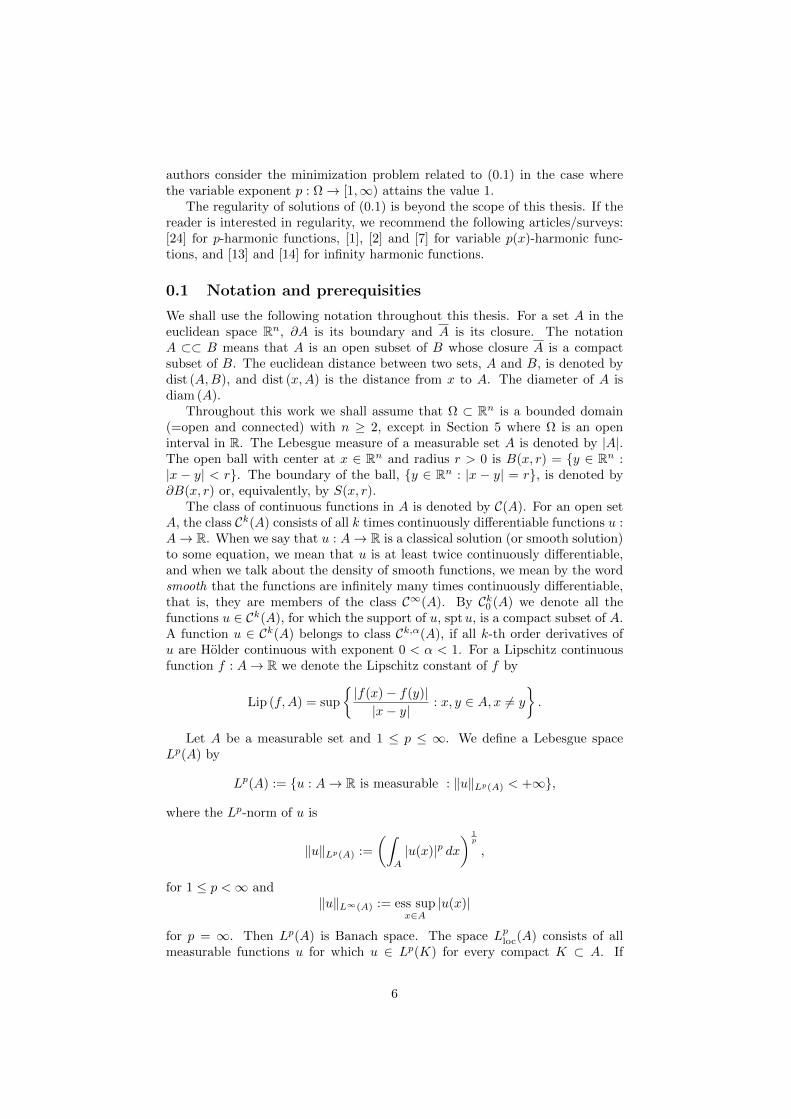
Theorem 2.8. Let upk∞k=1 be a family of pk-harmonic functions such thatupk → u locally uniformly in Ω as pk →∞. Then u is infinity harmonic.

Proof. We show that the function u is a viscosity supersolution of −∆∞u = 0.The proof that u is a subsolution is similar.

Let ϕ ∈ C2(Ω) and x ∈ Ω such that u−ϕ has a strict minimum at x. Withoutloss of generality, we may assume that (u − ϕ)(x) = 0. Let r > 0 be such thatB(x, r) ⊂ Ω and define

mr := min u(x)− ϕ(x) : |x− x| = r > 0,

andεk,r := sup upk(x)− u(x) : |x− x| ≤ r > 0

for k ∈ N. Choose k1 = k1(r) ∈ N such that εk,r <mr

2 when k ≥ k1. Now

infB(x,r)

(upk − ϕ) ≤ upk(x)− ϕ(x) = upk(x)− u(x) ≤ εk,r <mr

2

andinfS(x,r)

(upk − ϕ) ≥ mr − εk,r > mr −mr

2=mr

2

holds for any k ≥ k1. This means that for large k the function upk − ϕ attainsits local minimum inside the ball B(x, r). We fix such a point and denote it byxk.

Next we show that xk → x. This is done by repeating the previous procedurefor smaller radii. For example, we find k2 = k2(r/2) such that if k ≥ k2; thenthe function upk − ϕ attains its local minimum at xk ∈ B(x, r/2). By choosingxk ∈ B(x, r) for k1 ≤ k < k2, xk ∈ B(x, r/2) for k2 ≤ k < k3 = k3(r/3) and soon, we find a sequence (xk)∞k=1 for which xk → x.

Now, by Lemma 2.7, it holds that

−(|∇ϕ(xk)|pk−2∆ϕ(xk) + (pk − 2)|∇ϕ(xk)|pk−4∆∞ϕ(xk)

)≥ 0.

If ∇ϕ(x) = 0, then −∆∞ϕ(x) = 0, and we are done. Thus we can assume that∇ϕ(x) 6= 0. Then ∇ϕ(xk) 6= 0 for large k by the continuity of ∇ϕ. We dividethe previous inequality by |∇ϕ(xk)|pk−4(pk − 2) and get

−|∇ϕ(xk)|2∆ϕ(xk)

pk − 2−∆∞ϕ(xk) ≥ 0.

Letting k →∞ and, consequently, pk →∞, we obtain

−∆∞ϕ(x) ≥ 0,

which proves the claim.

17

2.2 Uniqueness of solutions

The uniqueness of the solution of (2.2) follows immediately from the next the-orem. It is due to Jensen [21], but we follow a recently published new proof byArmstrong and Smart [3].

Theorem 2.9. Let u, v ∈ C(Ω) such that u is infinity subharmonic and v isinfinity superharmonic. Then

maxΩ

(u− v) = max∂Ω

(u− v).

We now introduce some notation. For ε > 0 we write Ωε := x ∈ Ω :B(x, ε) ⊂ Ω. If u ∈ C(Ω) and x ∈ Ωε, then we denote

S+ε u(x) := max

y∈B(x,ε)

u(y)− u(x)

ε

and

S−ε u(x) := maxy∈B(x,ε)

u(x)− u(y)

ε.

By choosing y = x, we see that S+ε u(x), S−ε u(x) ≥ 0.

The next result is a comparison lemma for a finite difference equation andit is a first step towards the proof of Theorem 2.9.

Lemma 2.10. Suppose that u, v ∈ C(Ω) ∩ L∞(Ω) and

S−ε u(x)− S+ε u(x) ≤ 0 ≤ S−ε v(x)− S+

ε v(x) (2.4)

holds for every x ∈ Ωε. Then

supΩ

(u− v) = supΩ\Ωε

(u− v).

Proof. We prove by contradiction. Suppose that

supΩ

(u− v) > supΩ\Ωε

(u− v).

Then the setE := x ∈ Ω : (u− v)(x) = sup

Ω(u− v)

is nonempty, compact and E ⊂ Ωε. Let

F := x ∈ E : u(x) = maxE

u

and choose a point x0 ∈ ∂F . Then x0 ∈ E, which means that u− v attains itsmaximum at x0. In particular, this means that for every x ∈ B(x0, ε) it holdsthat u(x)− v(x) ≤ u(x0)− v(x0), and hence

v(x0)− v(x)

ε≤ u(x0)− u(x)

ε≤ S−ε u(x0).

This implies thatS−ε v(x0) ≤ S−ε u(x0). (2.5)

18

If it was the case that S+ε u(x0) = 0, then by (2.4), (2.5) and the non-

negativeness of S+ε and S−ε it would hold that

S−ε u(x0) = S+ε u(x0) = 0 = S−ε v(x0) = S+

ε v(x0).

Hence u(x) ≡ u(x0) and v(x) ≡ v(x0) in the ball B(x0, ε). Since x0 ∈ ∂F ,there exists y ∈ B(x0, ε) \ F . If y ∈ E, then u(y) < maxE u = u(x0), which isa contradiction since u was supposed to be a constant in the ball B(x0, ε). Ify /∈ E, then (u−v)(y) < supΩ (u−v) = (u−v)(x0), which is also a contradictionsince u− v was supposed to be a constant in B(x0, ε). This yields that the caseS+ε u(x0) = 0 is not possible.

Now we consider the case S+ε u(x0) > 0. Since u is continuous and B(x0, ε)

is compact, there exists z ∈ B(x0, ε) such that

S+ε u(x0) =

u(z)− u(x0)

ε.

This implies thatu(z) = u(x0) + εS+

ε u(x0)︸ ︷︷ ︸>0

> u(x0).

If z ∈ E, then u(z) > u(x0) = maxE u, which is a contradiction. Thus z /∈ E,and it holds that (u−v)(z) < (u−v)(x0). From this we get that v(z)−v(x0) >u(z)− u(x0), and thus

εS+ε v(x0) ≥ v(z)− v(x0) > u(z)− u(x0) = εS+

ε u(x0),

which yields−S+

ε v(x0) < −S+ε u(x0). (2.6)

Combining (2.5) and (2.6), we have that

S−ε v(x0)− S+ε v(x0) < S−ε u(x0)− S+

ε u(x0),

which contradicts (2.4), and the claim follows.

We continue by presenting new notations. For u ∈ C(Ω) and x ∈ Ωε we write

uε(x) := maxy∈B(x,ε)

u(y)

anduε(x) := min

y∈B(x,ε)u(y).

ThenεS+

ε u(x) = maxy∈B(x,ε)

(u(y)− u(x)) = uε(x)− u(x)

andεS−ε u(x) = max

y∈B(x,ε)(u(x)− u(y)) = u(x)− uε(x).

These notations are used in the next Lemma, which allows us to modify thesolutions of the PDE (2.2) to get solutions that satisfy (2.4). Before we proceedto this Lemma, we present a property called Comparison with cones, which istightly related to infinity harmonic functions and which is needed in the proofof the Lemma.

19

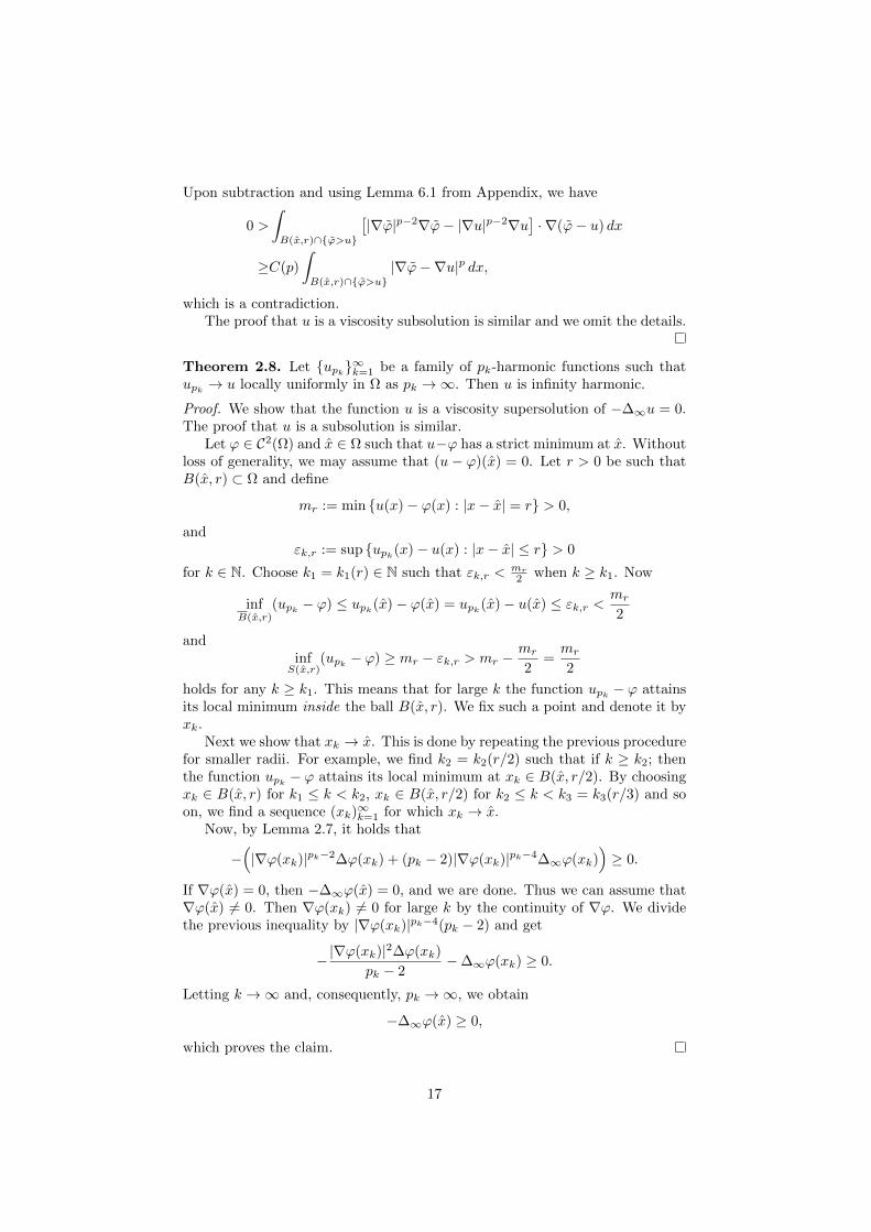
Definition 2.11. The function u : Ω → R enjoys comparison with cones fromabove in Ω, if for every open set U ⊂⊂ Ω and every x0 ∈ Rn, a, b ∈ R, for which

u(x) ≤ C(x) = a+ b|x− x0| (2.7)

holds for every x ∈ ∂(U \ x0); one then has

u(x) ≤ C(x)

also for every x ∈ U .Comparison with cones from below is defined similarly, that is, ” ≤ ” is

replaced by ” ≥ ”. Moreover, we say that u enjoys comparison with cones in Ωif u enjoys comparison with cones both from above and below.

Theorem 2.12. Assume that u is an infinity subharmonic (superharmonic,respectively) function in Ω. Then u enjoys comparison with cones from above(below) in Ω.

Proof. Let U ⊂⊂ Ω be open and x0 ∈ Rn, a, b ∈ R be such that u ≤ C on∂(U \ x0). Assume, on the contrary, that there exists x ∈ U \ x0 such thatu(x) > C(x). Let R > 0 be so large that x0 ∈ B(x,R) for every x ∈ ∂U and set

w(x) := a+ b|x− x0|+ ε(R2 − |x− x0|2), x ∈ U.

Then u ≤ w on ∂(U \ x0) but u(x) > w(x) when ε > 0 is small enough. Wemay assume that x is the maximum point of u−w in U \ x0. One calculatesthat

−∆∞w(x) = 2ε(2ε|x− x0|2 − b)2.

This is strictly positive if b ≤ 0 or if b > 0 and ε is small enough. Thisis a contradiction to our assumption that u is infinity subharmonic, that is,−∆∞u ≤ 0.

Lemma 2.13. Suppose that u and v are infinity subharmonic and superhar-monic functions in Ω, respectively. Then

S−ε uε(x)− S+

ε uε(x) ≤ 0 (2.8)

andS−ε vε(x)− S+

ε vε(x) ≥ 0 (2.9)

for all x ∈ Ω2ε.

Proof. We first prove (2.8). Let x0 ∈ Ω2ε. Choose y0 ∈ B(x0, ε) and z0 ∈B(x0, 2ε) such that u(y0) = uε(x0) and u(z0) = u2ε(x0). Since

(uε)ε

(x0) = maxy∈B(x0,ε)

uε(y) = maxy∈B(x0,ε)

maxz∈B(y,ε)

u(z) = u2ε(x0)

and(uε)ε (x0) = min

y∈B(x0,ε)uε(y) = min

y∈B(x0,ε)max

z∈B(y,ε)u(z) ≥ u(x0),

20

we have that

ε(S−ε u

ε(x0)− S+ε u

ε(x0))

= uε(x0)− (uε)ε (x0)− ((uε)ε

(x0)− uε(x0))

= 2uε(x0)− (uε)ε

(x0)− (uε)ε (x0)

≤ 2uε(x0)− u2ε(x0)− u(x0) (2.10)

= 2u(y0)− u(z0)− u(x0).

By the definition of z0 it is easy to see that the inequality

u(w) ≤ u(x0) +u(z0)− u(x0)

2ε|w − x0| (2.11)

holds for every w ∈ ∂ (B(x0, 2ε) \ x0), (that is, |w − x0| = 2ε or w = x0).Since u is an infinity subharmonic function, Theorem 2.12 implies that (2.11)holds also for every w ∈ B(x0, 2ε). This allows to put w = y0 to (2.11), and weget

u(y0) ≤ u(x0) +u(z0)− u(x0)

2ε|y0 − x0|

≤ u(x0) +u(z0)− u(x0)

2εε

=1

2u(x0) +

1

2u(z0).

From this we deduce that 2u(y0)−u(z0)−u(x0) ≤ 0, which together with (2.10)yields

S−ε uε(x0)− S+

ε uε(x0) ≤ 0.

Since x0 ∈ Ω2ε was arbitrary, the proof of (2.8) is complete.To prove (2.9), we substitute −v, which is an infinity subharmonic function

in Ω, with (2.8) and use the facts that S+ε (−v)(x) = S−ε v(x) and (−v)ε = −vε.

Indeed, for x ∈ Ω2ε, we calculate that

0 ≥ S−ε (−v)ε(x)− S+ε (−v)ε(x)

= S−ε (−vε)(x)− S+ε (−vε)(x)

= S+ε vε(x)− S−ε vε(x),

which is (2.9).

Proof of Theorem 2.9. By Lemmas 2.10 and 2.13

supΩε

(uε − vε) = supΩε\Ω2ε

(uε − vε)

for all ε > 0. Let ε→ 0, and the claim follows.

Let us briefly discuss the necessity of the assumption that the boundarydata is Lipschitz continuous. We used this assumption in the proof of existence,for simplicity, but it turns out that it is not crucial and it can be relaxed tocontinuity, see [21]. In the proof of uniqueness we did not use the Lipschitzcontinuity. Thus Theorem 2.4 is true if the boundary data is just continuous.

We also want to remark that Theorem 2.9 implies that the entire sequence(up)p, which was used in the existence part, converges uniformly in Ω.

21

2.3 Minimizing property and related topics

Theorem 1.5 shows the equivalence of p-harmonic functions and the energyminimizers. In this section we discuss the analogous result for p =∞.

First we define what it means to be a minimizer in the case p =∞.

Definition 2.14. A function u ∈ W 1,∞loc (Ω) satisfies the AMG (absolutely

minimizing gradient) property in Ω if for every open U ⊂⊂ Ω and for everyv ∈W 1,∞

loc (Ω) with v = u on ∂U we have that

‖∇u‖L∞(U) ≤ ‖∇v‖L∞(U).

As can be seen from [4], the need for a local minimizing property is justified.To be exact, it could be possible to have multiple functions with given boundarydata that minimize the norm of the gradient in whole Ω. To gain uniqueness,we need to add an extra condition, which is that the minimizer must also bea local minimizer. In a p-harmonic case we do not need this extra condition,since a global minimizer is also a local minimizer, due to the set additivity ofthe integral. In fact, the AMG property is derived from this p-harmonicity bysending p→∞.

Now we show that infinity harmonic functions are the same as the functionsthat satisfy the AMG property. This is done by using comparison with cones,which was presented before. The next theorem says that all these propertiesare equivalent.

Theorem 2.15. Let u ∈ W 1,∞loc (Ω). Then the following conditions are equiva-

lent:

(a) u satisfies the AMG property in Ω.

(b) u enjoys comparison with cones in Ω.

(c) u is infinity harmonic in Ω.

Proof. “(c) =⇒ (b)”: This is Theorem 2.12. “(b) =⇒ (a)”: We omit theproof of this implication, since the proof is quite long and it is based on severaltechnical lemmas, see [9, Theorem 3.2]. “(b) =⇒ (c)”: Suppose that (c) isnot true. We may assume that u is not infinity subharmonic in Ω, that is, thereexist ϕ ∈ C2(Ω) and x ∈ Ω such that u − ϕ attains its local zero maximum atx, but −∆∞ϕ(x) > 0.

By Lemma 6.3 in the Appendix, there exists a cone function C such that

(i) C(x) = ϕ(x)

(ii) ∇C(x) = ∇ϕ(x)

(iii) D2C(x) > D2ϕ(x),

where the third statement means that

D2C(x)ξ · ξ > D2ϕ(x)ξ · ξ for all ξ ∈ Rn \ 0.

This means that x is a strict local maximum point for the function ϕ− C, andhence it is possible to find r1 > 0 such that

ϕ(x)− C(x) < ϕ(x)− C(x) = 0

22

for every x ∈ B(x, r1) \ x. Further, by antithesis, there exists r2 > 0 suchthat

u(x)− ϕ(x) ≤ 0

in a ball B(x, r2). These inequalities together yield

u(x)− C(x) < 0

for all x ∈ B(x, r) \ x, where r = minr1, r2. This allows us to find ε > 0such that

maxx∈∂B(x,r)

(u(x)− C(x)) < −ε.

Now for the cone C − ε it holds that

u(x) ≤ C(x)− ε (2.12)

for every x ∈ ∂B(x, r). Since u enjoys comparison with cones, (2.12) holds alsofor every x ∈ B(x, r). This is a contradiction since C(x)− ε = u(x)− ε < u(x).

“(a) =⇒ (b)”: Suppose that u does not enjoy comparison with conesfrom above. Then there exist U ⊂⊂ Ω, x0 ∈ Rn and a, b ∈ R such thatu(x) ≤ C(x) := a+ b|x− x0| on ∂ (U \ x0) but u(x) > C(x) for some x ∈ U .

Consider a half-line that has endpoint at x0 and which passes through x,and pick two distinct points y1 and y2 from that half-line such that y1, y2 ∈∂(U \ x0) and the segment ]y1, y2[ lies in U . For identification, we assumethat y1 is the point which is located between x0 and x. Let yj,δ = yj +δ(x−yj),0 < δ < 1, for j = 1, 2. Since u satisfies the AMG property in Ω, we have that

‖∇u‖L∞(U) ≤ ‖∇(a+ b|x− x0|)‖L∞(U) = |b|,

and thus|u(yj,δ)− u(yj)| ≤ |b||x− yj |δ.

If b ≥ 0, then

u(y1,δ) ≤ u(y1) + b|x− y1|δ ≤ a+ b|y1 − x0|+ b|x− y1|δ.

As δ → 1, u(y1,δ) → u(x) and a + b|y1 − x0| + b|x − y1|δ → C(x), whichcontradicts the assumption u(x) > C(x). If b < 0, then

u(y2,δ) ≤ u(y2)− b|x− y2|δ ≤ a+ b|y2 − x0| − b|x− y2|δ

When δ → 1, u(y2,δ)→ u(x) and a+ b|y2 − x0| − b|x− y2|δ → C(x), which alsocontradicts with u(x) > C(x).

We can similarly prove that u enjoys comparison with cones from below.

23

3 Variable p(x), with 1 < inf p(x) < sup p(x) < +∞In this section we let a (measurable) function p : Ω→ (1,∞] vary in the set Ω.The function p is called a variable exponent. We set

p− := infx∈Ω

p(x) and p+ := supx∈Ω

p(x)

and assume that1 < p− < p+ < +∞.

The variable exponent Lebesgue space Lp(·)(Ω) consists of all measurablefunctions u defined on Ω for which∫

Ω

|u(x)|p(x) dx < +∞.

The Luxembourg norm on this space is defined as

‖u‖Lp(·)(Ω) := inf

λ > 0 :

∫Ω

∣∣∣∣u(x)

λ

∣∣∣∣p(x)

dx ≤ 1

.

Equipped with this norm, Lp(·)(Ω) is a Banach space. If p is a constant function,then the variable exponent Lebesgue space is just the standard Lebesgue space.

The following properties are needed later (for the proof, see [15]); for u ∈Lp(·)(Ω) it holds that

(i) if ‖u‖Lp(·)(Ω) < 1, then ‖u‖p+

Lp(·)(Ω)≤∫

Ω|u(x)|p(x) dx ≤ ‖u‖p−

Lp(·)(Ω),

(ii) if ‖u‖Lp(·)(Ω) > 1, then ‖u‖p−Lp(·)(Ω)

≤∫

Ω|u(x)|p(x) dx ≤ ‖u‖p

+

Lp(·)(Ω),

(iii) ‖u‖Lp(·)(Ω) = 1 if and only if∫

Ω|u(x)|p(x) dx = 1.

The outcome of these properties is

min‖u‖p

+

Lp(·)(Ω), ‖u‖p−

Lp(·)(Ω)

≤∫

Ω

|u(x)|p(x) dx (3.1)

≤ max‖u‖p

+

Lp(·)(Ω), ‖u‖p−

Lp(·)(Ω)

.

We also present a variable exponent version of Holder’s inequality:∫Ω

|fg| dx ≤ C‖f‖Lp(·)‖g‖Lq(·)

holds for f ∈ Lp(·)(Ω) and g ∈ Lq(·)(Ω), where C = C(p−, p+) and 1/p(x) +

1/q(x) = 1 for every x ∈ Ω. Moreover, the dual space of Lp(·)(Ω) is Lq(·)(Ω)and the space Lp(·)(Ω) is reflexive.

We continue by defining a variable exponent Sobolev space W 1,p(·)(Ω). Itconsists of functions u ∈ Lp(·)(Ω), whose weak gradient ∇u exists and belongsto Lp(·)(Ω). The space W 1,p(·)(Ω) is a reflexive Banach space with the norm

‖u‖W 1,p(·)(Ω) := ‖u‖Lp(·)(Ω) + ‖∇u‖Lp(·)(Ω).

24

The density of smooth functions in W 1,p(·)(Ω) is not a trivial issue and it canhappen that the smooth functions are not dense. However, if we assume thatthe variable exponent p is log-Holder -continuous, that is,

|p(x)− p(y)| ≤ C

log(e+ 1/|x− y|)(3.2)

for some C > 0 and for every x, y ∈ Ω, then smooth functions are dense inW 1,p(·)(Ω). To the best of our knowledge, this is the weakest modulus of con-tinuity for p that ensures the density of smooth functions in variable exponentSobolev spaces, see [26] and [11, Chapter 9]. From now on we assume that (3.2)holds.

Under the assumption that C∞(Ω) is dense in W 1,p(·)(Ω), the variable ex-

ponent Sobolev space with zero boundary values, W1,p(·)0 (Ω), is defined as the

closure of C∞0 (Ω) with respect to the norm ‖·‖W 1,p(·)(Ω), and it is reflexive. Tocheck the basic properties of the variable exponent Lebesgue and Sobolev spaces,see [15] and [23].

We also want to present the variable exponent Sobolev-Poincare inequality:

‖u‖Lp(·)(Ω) ≤ C(diam Ω)‖∇u‖Lp(·)(Ω)

holds for functions u ∈W 1,p(·)0 (Ω). Here C = C(n, p).

Remark 3.1. Generally, there are several sufficient assumptions for p so thatthe Sobolev-Poincare inequality holds. These include

• p is log-Holder continuous (our case)

• p satisfies a so-called jump condition in Ω: there exists δ > 0 such thatfor every x ∈ Ω either

ess inf p(y) : y ∈ B(x, δ) ≥ n

or

ess sup p(y) : y ∈ B(x, δ) ≤ n · ess inf p(y) : y ∈ B(x, δ)n− ess inf p(y) : y ∈ B(x, δ)

.

Note that if p is continuous up to the boundary, then p satisfies the jump-condition.

For the references, see [11] and [17].

We proceed as in the constant p-case. The methods are the same, only inthe proofs we need to be more accurate. We start by defining a p(x)-harmonicfunction.

Definition 3.2. We say that a function u ∈ W1,p(·)loc (Ω) is a weak solution

(respectively, subsolution, supersolution) of

−∆p(x)u = − div(|∇u(x)|p(x)−2∇u(x)

)= 0 (3.3)

in Ω, if ∫Ω

|∇u(x)|p(x)−2∇u(x) · ∇ϕ(x) dx = 0 (respectively, ≤ 0, ≥ 0)

25

for every test function ϕ ∈ C∞0 (Ω) (respectively, for every non-negative testfunction ϕ ∈ C∞0 (Ω)).

A continuous weak solution of −∆p(x)u = 0 is called a p(x)-harmonic func-tion.

As in the constant p-case, the continuity requirement for a p(x)-harmonicfunction is redundant. For higher regularity results, see [1], [7] and the listof references given in [11, Chapter 13]. Furthermore, the test function space

C∞0 (Ω) can be extended to W1,p(·)0 (Ω) if we assume that the p(x)-harmonic

function belongs to the class W 1,p(·)(Ω). This is based on the fact that C∞0 (Ω) is

dense in W1,p(·)0 (Ω) and on the variable exponent version of Holder’s inequality.

Calculations are the same as in Section 1 and will not be repeated.The next theorem is the p(x)-version of Theorem 1.3. This is our main goal

in this section.

Theorem 3.3. Let Ω ⊂ Rn be a bounded domain, p a log-Holder-continuousvariable exponent with 1 < p− < p+ < +∞ and f ∈ W 1,p(·)(Ω). Thenthere exists a unique p(x)-harmonic function u ∈ W 1,p(·)(Ω) such that u− f ∈W

1,p(·)0 (Ω), that is, u is a weak solution of

−∆p(x)u = 0, in Ω,

u = f, on ∂Ω.(3.4)

For the proof we define a functional I : W 1,p(·)(Ω)→ R,

I(u) =

∫Ω

1

p(x)|∇u(x)|p(x) dx.

Then (3.3) is the Euler-Lagrange equation of the functional I. The existenceand uniqueness of solutions of (3.4) is obtained by the following two theorems,just as in the constant p-case.

Theorem 3.4. Let f ∈ W 1,p(·)(Ω) be the boundary data. Then the following

conditions are equivalent for u ∈W 1,p(·)f (Ω):

(a) −∆p(x)u = 0 in Ω,

(b) I(u) ≤ I(v) for every v ∈W 1,p(·)f (Ω).

Theorem 3.5. Let f ∈W 1,p(·)(Ω) be the boundary data. There exists a unique

u ∈W 1,p(·)f (Ω) such that∫

Ω

1

p(x)|∇u(x)|p(x) dx ≤

∫Ω

1

p(x)|∇v(x)|p(x) dx

for every v ∈W 1,p(·)f (Ω).

Now we try to modify the proofs from Section 1 to fit to the p(x)-case.

Proof of Theorem 3.4. ”(a) =⇒ (b)”: Let v ∈W 1,p(·)f (Ω). For any fixed x0 ∈ Ω

the function y → |y|p(x0) is convex, and thus

|∇v(x)|p(x0) ≥ |∇u(x)|p(x0) + p(x0)|∇u(x)|p(x0)−2∇u(x) · (∇v(x)−∇u(x))

26

holds for every x ∈ Ω, especially for x = x0. Since x0 ∈ Ω was arbitrary, wehave

|∇v(x)|p(x) ≥ |∇u(x)|p(x) + p(x)|∇u(x)|p(x)−2∇u(x) · (∇v(x)−∇u(x)).

We divide by p(x) and integrate over Ω, and the result is∫Ω

1

p(x)|∇v(x)|p(x) dx ≥

∫Ω

1

p(x)|∇u(x)|p(x) dx (3.5)

+

∫Ω

|∇u(x)|p(x)−2∇u(x) · (∇v(x)−∇u(x)) dx.

Since u is p(x)-harmonic and belongs to the class W 1,p(·)(Ω), the function v−u ∈W

1,p(·)0 (Ω) is an admissible function to test the p(x)-harmonicity of u, and thus

the last integral is zero. This implies that I(u) ≤ I(v).

”(b) =⇒ (a)”: Assume that u ∈ W 1,p(·)f (Ω) is the minimizer for the func-

tional I. Fix ϕ ∈ C∞0 (Ω) and set ut(x) = u(x) + tϕ(x). Then ut ∈ W 1,p(·)f (Ω)

and I(u) = I(u0) ≤ I(ut) for all t ∈ R. Hence

0 = limt→0

I(ut)− I(u)

t= limt→0

∫Ω

1

p(x)

|∇ut(x)|p(x) − |∇u(x)|p(x)

tdx

=

∫Ω

1

p(x)limt→0

|∇ut(x)|p(x) − |∇u(x)|p(x)

tdx

=

∫Ω

1

p(x)

d

dt

[|∇ut(x)|p(x)

]t=0

dx

=

∫Ω

1

p(x)p(x)

[(∇u(x) + t∇ϕ(x))|∇u(x) + tϕ(x)|p(x)−2 · ∇ϕ(x)

]t=0

dx

=

∫Ω

|∇u(x)|p(x)−2∇u(x) · ∇ϕ(x) dx.

If we can show why the third equality is true, the proof is complete sincethe other equalities are clear. To do this, we set

ft(x) =|∇ut(x)|p(x) − |∇u0(x)|p(x)

t

and use the mean value theorem to get the following estimate: there existss ∈ R, 0 < |s| < |t| < 1 such that

ft(x) =|∇u0(x) + t∇ϕ(x)|p(x) − |∇u0(x)|p(x)

t

= p(x)|s∇ϕ(x) +∇u0(x)|p(x)−2 (s∇ϕ(x) +∇u0(x)) · ∇ϕ(x),

and then

|ft(x)| ≤ p+‖∇ϕ‖L∞(Ω)|s∇ϕ(x) +∇u0(x)|p(x)−1

≤ C(ϕ)p+2p(x)−1(sp(x)−1|∇ϕ(x)|p(x)−1 + |∇u0(x)|p(x)−1)

≤ C(ϕ)p+2p+−1(max1, ‖∇ϕ‖p

+−1L∞(Ω)+ |∇u0(x)|p(x)−1)

= C(ϕ, p)(C(ϕ, p) + |∇u0(x)|p(x)−1).

27

Then by the variable exponent version of Holder’s inequality we have∫Ω

|ft(x)| dx ≤ C(ϕ, p)

(C(ϕ, p)|Ω|+

∫Ω

|∇u0(x)|p(x)−1 · 1 dx)

≤ C(ϕ, p)

(C(ϕ, p)|Ω|+ C(p)‖|∇u0|p(·)−1‖

Lp(·)

p(·)−1 (Ω)‖1‖Lp(·)(Ω)

).

Since ∫Ω

(|∇u0(x)|p(x)−1

) p(x)p(x)−1

dx =

∫Ω

|∇u0(x)|p(x) dx < +∞,

we have |∇u0|p(·)−1 ∈ Lp(·)

p(·)−1 (Ω) and thus ‖|∇u0|p(·)−1‖L

p(·)p(·)−1 (Ω)

< +∞. It fol-

lows that ft has an L1-integrable majorant, and then, by Lebesgue’s dominatedconvergence theorem,

limt→0

∫Ω

ft(x) dx =

∫Ω

limt→0

ft(x) dx.

This completes the proof.

Remark 3.6. Using the same argument as at the beginning of the proof ofTheorem 3.4, we have for u, v ∈ Lp(·)(Ω) that

|tu(x) + (1− t)v(x)|p(x) ≤ t|u(x)|p(x) + (1− t)|v(x)|p(x) (3.6)

for every 0 ≤ t ≤ 1 and every x ∈ Ω. Since p− > 1, the inequality is strict if|x ∈ Ω : u(x) 6= v(x)| > 0.

Moreover, since the mapping F : Ω × Rn → R, where F (x, ξ) = 1p(x) |ξ|

p(x),

is C1-smooth and ξ 7→ F (x, ξ) is convex for every x ∈ Ω by (3.6), the functionalI is weakly lower semicontinuous, see [16].

Although the next proof is mainly similar to the proof of Theorem 1.4, thereare slight differences that come from the p(x)-term. To point this out, we repeatthe proof.

Proof of Theorem 3.5. Let

I0 = infv∈W 1,p(·)

f (Ω)

∫Ω

1

p(x)|∇v(x)|p(x) dx.

Then

0 ≤ I0 ≤∫

Ω

1

p(x)|∇f(x)|p(x) dx ≤ 1

p−

∫Ω

|∇f(x)|p(x) dx < +∞.

This allows us to choose a sequence of functions v1, v2, v3, ... ∈ W 1,p(·)f (Ω) such

that ∫Ω

1

p(x)|∇vj(x)|p(x) dx < I0 +

1

j

28

for j = 1, 2, 3, ... Since vj − f ∈ W1,p(·)0 (Ω), we find by the Sobolev-Poincare

inequality that

‖vj‖Lp(·)(Ω) ≤ ‖vj − f‖Lp(·)(Ω) + ‖f‖Lp(·)(Ω)

≤ C(n, p)‖∇vj −∇f‖Lp(·)(Ω) + ‖f‖Lp(·)(Ω)

≤ C(n, p)‖∇vj‖Lp(·)(Ω) + C(n, p)‖∇f‖Lp(·)(Ω) + ‖f‖Lp(·)(Ω) (3.7)

≤ C(n, p)‖∇vj‖Lp(·)(Ω) + C(n, p)‖f‖W 1,p(·)(Ω).

We next estimate the term ‖∇vj‖Lp(·)(Ω). If ‖∇vj‖Lp(·)(Ω) > 1, then

‖∇vj‖Lp(·)(Ω) =(‖∇vj‖p−Lp(·)(Ω)

) 1p− ≤

(∫Ω

|∇vj(x)|p(x) dx

) 1p−

≤(p+

∫Ω

1

p(x)|∇vj(x)|p(x) dx

) 1p−

≤(p+(I0 +

1

j)

) 1p−≤(p+(I0 + 1)

) 1p− .

If ‖∇vj‖Lp(·)(Ω) ≤ 1, then no estimates are needed. Hence we get

‖∇vj‖Lp(·)(Ω) ≤ 1 +(p+(I0 + 1)

) 1p− (3.8)

for every j = 1, 2, 3, ... Now (3.7) together with (3.8) gives that the sequence(vj)

∞j=1 is bounded in W 1,p(·)(Ω). Then there exists a subsequence, still denoted

as (vj)∞j=1, and u0 ∈ W 1,p(·)

f (Ω) such that vj u0 weakly in W 1,p(·)(Ω). Theweak lower semicontinuity of the functional I implies that

I0 ≤ I(u0) ≤ lim infj→∞

I(vj) = I0.

This proves the existence.To prove the uniqueness, we assume that u1 and u2 are two minimizers.

Then u = u1+u2

2 ∈W 1,p(·)f (Ω), and we have

I0 ≤∫

Ω

1

p(x)|∇u(x)|p(x) dx =

∫Ω

1

p(x)

∣∣∣∣∇u1(x) +∇u2(x)

2

∣∣∣∣p(x)

dx

(?) ≤∫

Ω

1

p(x)

|∇u1(x)|p(x) + |∇u2(x)|p(x)

2dx

=1

2

∫Ω

1

p(x)|∇u1(x)|p(x) dx+

1

2

∫Ω

1

p(x)|∇u2(x)|p(x) dx

=1

2I0 +

1

2I0 = I0.

In (?) we used convexity. If the measure of the set x ∈ Ω : ∇u1(x) 6= ∇u2(x)is positive, then the inequality (?) is strict by strict convexity, which leads to acontradiction. Thus ∇u1(x) = ∇u2(x) almost everywhere in Ω, and hence theSobolev-Poincare inequality implies that

‖u1 − u2‖Lp(·)(Ω) ≤ C‖∇u1 −∇u2‖Lp(·)(Ω) = 0.

Then u1 = u2, and the uniqueness follows.

29

4 Variable p(x) with p(·) ≡ +∞ in a subdomain

This section is based on [25] (an article by Manfredi, Rossi and Urbano), whichwas the first attempt to analyse the Dirichlet problem (0.1) in the case wherethe exponent p(·) becomes infinity in some part of the domain.

Let us fix the setting for this section. We assume that Ω ⊂ Rn and D ⊂ Ωare both bounded and convex domains with smooth boundaries, at least of classC1. The variable exponent p : Ω→ (1,∞] satisfies

p(x) = +∞ for every x ∈ D (4.1)

and is assumed to be continuously differentiable in Ω \D. We also assume thatboth functions p and ∇p have a continuous extension from Ω\D to ∂D∩Ω andthat

p− = infx∈Ω

p(x) > n (4.2)

andp+ := sup

x∈Ω\Dp(x) < +∞. (4.3)

In a way, the problem considered in this section is a combination of theproblems studied in the two previous sections. In the set D we have infinityharmonic functions (as in Section 2) and in the set Ω\D we have p(x)-harmonicfunctions (as in Section 3). However, we have extra assumptions for p, whichwe explain next.

Let us first compute how −∆p(x) (with p(x) < +∞ everywhere) evaluateson C2(Ω) functions. For ϕ ∈ C2(Ω) we find

−∆p(x)ϕ(x) =− div(|∇ϕ(x)|p(x)∇ϕ(x)

)=− |∇ϕ(x)|p(x)−2 (4.4)

×(

∆ϕ(x) +∇p(x) · ∇ϕ(x) log |∇ϕ(x)|+ (p(x)− 2)∆∞ϕ(x)

|∇ϕ(x)|2

).

In order to use the theory of viscosity solutions, the mapping x 7→ −∆p(x)ϕ(x)should be continuous. This is needed, for example, in Lemma 2.7. Since ∇pappears in (4.4), it is natural to assume that p ∈ C1(Ω \D). This also ensuresthe density of smooth functions in W 1,p(·)(Ω \D). That the functions p and ∇pcan be extended continuously from Ω \D to ∂D ∩Ω is needed to guarantee thecontinuity of the function x 7→ −∆p(x)ϕ(x) in Ω \D in the last theorem on thissection. The assumption (4.3) is there in order for us to use the theory fromSection 3, and the assumption (4.2) guarantees the continuous embedding; forthe variable exponent q : Ω→ [q−, q

+], n < q− < q+ < +∞, it holds that

W 1,q(·)(Ω) →W 1,q−(Ω) ⊂ C(Ω). (4.5)

The variable exponent q can even be discontinuous, and still (4.5) holds. Weshall use this embedding property later to bounded functions pk(x), wherepk(x) = min p(x), k, for which n < p− < pk(x) < p+ < +∞ holds in Ωfor large k. To check (4.5), see [23].

30

Remark 4.1. The convexity of Ω and D guarantees that the Lipschitz con-stant of W 1,∞-functions coincides with the L∞-norm of their gradients. Thisproperty is needed in some of the proofs. The boundary smoothness assumptionguarantees the existence of the exterior unit normal vector to ∂D in Ω, whichis also needed later.

The first step in trying to solve the Dirichlet boundary value problem,−∆p(x)u(x) = 0, if x ∈ Ω,

u(x) = f(x), if x ∈ ∂Ω,(4.6)

is to replace p(x) by a sequence of bounded functions pk(x) such that pk(x)is increasing in k and converges to p(x) as k → ∞. In this work we use thesequence where

pk(x) := min p(x), k.

We shall use the notation (4.6)k to refer to the problem (4.6) for the variableexponents pk(x).

Since p(x) is bounded in Ω \D, we have for large k that

pk(x) =

p(x), if x ∈ Ω \D,k, if x ∈ D.

Moreover, the boundary of the set x ∈ Ω : p(x) > k is ∂D for large k, andthus it is independent of k. This property is needed later in the proofs.

The next step is to solve (4.6)k. Since pk(x) is not log-Holder continuous,the existence and uniqueness do not follow from Theorem 3.3. However, Lemma4.3 below yields a solution to (4.6)k that we call uk. If we could show that thelimit limk→∞ uk exists, then it would be a natural candidate for a solution to(4.6) with the original p(x). The uniqueness is achieved quite easily; we combinethe results from Sections 2 and 3.

Before we formulate the main result, we introduce the sets in which theminimization process is done. For k ∈ N we define

Sk = u ∈W 1,pk(·)(Ω) : u|∂Ω = f

and

S = u ∈W 1,p−(Ω) : u|Ω\D ∈W1,p(·)(Ω \D), ‖∇u‖L∞(D) ≤ 1 and u|∂Ω = f.

Observe that S ⊂ Sk for every k ∈ N.

Theorem 4.2. Let p(·) be the variable exponent with the properties definedabove and f : ∂Ω → R a Lipschitz function. Then the following three claimsare true:

1) There exists a unique solution uk to (4.6)k.2) If S 6= ∅, then the uniform limit u∞ := lim

k→∞uk exists and it is a minimizer

of the variational integral ∫Ω\D

1

p(x)|∇u(x)|p(x) dx

31

in S. The function u∞ is the only minimizer amongst those functions in Sthat are also infinity harmonic in D in the viscosity sense. Moreover, u∞ is aviscosity solution of

−∆p(x)u(x) = 0, x ∈ Ω \D,−∆∞u(x) = 0, x ∈ D,sgn (|∇u|(x)− 1) sgn

(∂u∂ν (x)

)= 0, x ∈ ∂D ∩ Ω,

u(x) = f(x), x ∈ ∂Ω,

where ν is the exterior unit normal vector to ∂D in Ω.3) If ∂D ∩ ∂Ω 6= ∅ and the Lipschitz constant of f |∂D∩∂Ω is strictly greater

than one, then S = ∅ and

lim infk→∞

(∫D

|∇uk(x)|k

kdx

) 1k

> 1,

and hence the natural energy associated to the sequence (uk) is unbounded.

4.1 Approximate solutions uk

We first prove the existence and uniqueness of solutions to (4.6)k.

Lemma 4.3. Let p be the variable exponent as defined earlier and f : ∂Ω→ Ra Lipschitz function. Then, for k large enough, there exists a unique weaksolution uk ∈ W 1,pk(·)(Ω) to (4.6)k such that uk(x) = f(x) for every x ∈ ∂Ω.Moreover, uk is the unique minimizer of the functional

Ik(u) =

∫Ω

|∇u(x)|pk(x)

pk(x)dx =

∫Ω\D

|∇u(x)|p(x)

p(x)dx+

∫D

|∇u(x)|k

kdx

in Sk.

Proof. Suppose that k > p+. Then

pk(x) = mink, p(x) ≥ p− > n

for every x ∈ Ω. This ensures that pk satisfies the jump condition in Ω (seeRemark 3.1), and hence the Sobolev-Poincare inequality is applicable. Thismeans that the proof of Theorem 3.5 goes through with pk(x) and we find aunique minimizer uk for the functional Ik in Sk. By (4.5), uk is continuous upto the boundary and we can take the boundary condition pointwise.

Next we show that Theorem 3.4 holds for pk(x). The only difficulty we face

is the density of C∞0 (Ω) functions in W1,pk(·)0 (Ω). Since D is convex, it is a so-

called exterior cone domain and thus by the results of [12] and [20], the densityof smooth functions in W 1,pk(·)(Ω) follows from the corresponding densities inW 1,k(D) and W 1,p(·)(Ω \ D) which are known. We deduce that uk is also aunique weak solution of (4.6)k.

The problem (4.6)k is considered in the weak sense since the solutions neednot be smooth. Next we derive an equivalent formulation to the problem (4.6)k.Let us first suppose that u = uk ∈ C2(Ω). We set F : Ω× Rn → Rn, F (x, ξ) =

32

|ξ|pk(x)−2ξ and denote Fk := F |D×Rn and Fp(x) := F |Ω\D×Rn . We take ϕ ∈C∞0 (Ω) and calculate

div (F (x,∇u)ϕ) = [divF (x,∇u)]ϕ+ F (x,∇u) · ∇ϕ.

Then by the divergence theorem it holds that∫D

F (x,∇u) · ∇ϕdx

=

∫D

div[Fk(x,∇u)ϕ] dx−∫D

[divFk(x,∇u)]ϕdx

=

∫sptϕ∩D

div[Fk(x,∇u)ϕ] dx−∫D

[divFk(x,∇u)]ϕdx

=

∫∂(sptϕ∩D)

[Fk(x,∇u) · ν]ϕdS −∫D

[divF (x,∇u)]ϕdx

=

∫∂D∩Ω

[Fk(x,∇u) · ν]ϕdS −∫D

[divFk(x,∇u)]ϕdx,

and, similarly,∫Ω\D

F (x,∇u) · ∇ϕdx

=

∫Ω\D

div[Fp(x)(x,∇u)ϕ] dx−∫

Ω\D[divFp(x)(x,∇u)]ϕdx

=−∫∂D∩Ω

[Fp(x)(x,∇u) · ν]ϕdS −∫

Ω\D[divFp(x)(x,∇u)]ϕdx.

Hence,∫Ω

F (x,∇u) · ∇ϕdx =

∫∂D∩Ω

[Fk(x,∇u) · ν]ϕdS −∫∂D∩Ω

[Fp(x)(x,∇u) · ν]ϕdS

(4.7)

−∫D

[divFk(x,∇u)]ϕdx−∫

Ω\D[divFp(x)(x,∇u)]ϕdx.

Since u is a smooth solution, we have that

divFk(x,∇u) = 0

in D anddivFp(x)(x,∇u) = 0

in Ω \D, and thus∫Ω

F (x,∇u) · ∇ϕdx =

∫∂D∩Ω

[Fk(x,∇u) · ν]ϕdS −∫∂D∩Ω

[Fp(x)(x,∇u) · ν]ϕdS.

(4.8)Generally, u need not be smooth. Then the natural interpretation (in the

weak sense) of (4.7) is (4.8) for a solution u. This yields that∫Ω

F (x,∇u) · ∇ϕdx = 0

33

if and only if∫∂D∩Ω

[Fk(x,∇u) · ν]ϕdS =

∫∂D∩Ω

[Fp(x)(x,∇u) · ν]ϕdS

for every ϕ ∈ C∞0 (Ω). The latter equality is the interpretation of

|∇u(x)|k−2 ∂u

∂ν(x) = |∇u(x)|p(x)−2 ∂u

∂ν(x) for x ∈ ∂D ∩ Ω

in the weak sense.We get the following lemma.

Lemma 4.4. Problem (4.6)k is equivalent to the problem−∆p(x)uk(x) = 0, x ∈ Ω \D,−∆kuk(x) = 0, x ∈ D,|∇uk(x)|k−2 ∂uk

∂ν (x) = |∇uk(x)|p(x)−2 ∂uk

∂ν (x), x ∈ ∂D ∩ Ω,

uk(x) = f(x), x ∈ ∂Ω.

(4.9)

Here ν is the exterior unit normal vector to ∂D in Ω.

Remark 4.5. From now on, if u is smooth, we may write −∆pk(x)u(x) as

• −∆p(x)u(x), if x ∈ Ω \D

• −∆ku(x), if x ∈ D

• |∇uk(x)|k−2 ∂uk

∂ν (x)− |∇uk(x)|p(x)−2 ∂uk

∂ν (x), if x ∈ ∂D ∩ Ω.

The next step is to show that weak solutions uk of (4.6)k are also viscositysolutions of the same problem. This result is similar to Lemma 2.7, but we needto pay extra attention when considering the equation on ∂D ∩ Ω. Before thatwe define viscosity solutions of the equation −∆pk(·)u = 0.

Definition 4.6. i) An upper semicontinuous function u : Ω→ R is a viscositysubsolution of −∆pk(·)u = 0 in Ω if for every local maximum point x ∈ Ω of

u − ϕ, where ϕ ∈ C2(Ω), we have −∆p(x)ϕ(x) ≤ 0 if x ∈ Ω \D, −∆kϕ(x) ≤ 0

if x ∈ D, and the minimum of −∆p(x)ϕ(x), −∆kϕ(x), |∇ϕ(x)|k−2 ∂ϕ∂ν (x) −

|∇ϕ(x)|p(x)−2 ∂ϕ∂ν (x) ≤ 0 if x ∈ ∂D ∩ Ω.

ii) A lower semicontinuous function u : Ω → R is a viscosity supersolu-tion of −∆pk(·)u = 0 in Ω if for every local minimum point x ∈ Ω of u − ϕ,

where ϕ ∈ C2(Ω), we have −∆p(x)ϕ(x) ≥ 0 if x ∈ Ω \ D, −∆kϕ(x) ≥ 0

if x ∈ D, and the maximum of −∆p(x)ϕ(x), −∆kϕ(x), |∇ϕ(x)|k−2 ∂ϕ∂ν (x) −

|∇ϕ(x)|p(x)−2 ∂ϕ∂ν (x) ≥ 0 if x ∈ ∂D ∩ Ω.

iii) We say that a function u ∈ C(Ω) is a viscosity solution of −∆pk(·)u = 0in Ω if it is both a viscosity sub- and supersolution in Ω.

At this point we want to remark that, as in Remark 2.3, the local maximaand minima of u − ϕ can be assumed to be strict and/or global maxima andminima.

Lemma 4.7. Let uk be a continuous weak solution of (4.6)k. Then uk is alsoa viscosity solution of (4.6)k.

34

Proof. To prove the lemma, we need to show that uk is a viscosity solution of−∆pk(·)u = 0 in Ω and that uk(x) = f(x) for every x ∈ ∂Ω. First we notice thatthe boundary condition is true by Lemma 4.3. We prove that uk is a viscositysupersolution of −∆pk(·)u = 0 in Ω. The proof that uk is a viscosity subsolutionis similar, and we omit the details.

To check that the condition in Definition 4.6 ii) holds, we argue by contra-diction. Suppose that there exist x ∈ Ω and ϕ ∈ C2(Ω) such that uk−ϕ attainsits strict minimum at x and −∆pk(x)ϕ(x) < 0. Without loss of generality wemay assume that (uk − ϕ)(x) = 0. Depending on the location of x, we havethree cases.

Case 1. x ∈ Ω \D. Then the counter-assumption becomes

−∆p(x)ϕ(x) =− |∇ϕ(x)|p(x)−2∆ϕ(x)− (p(x)− 2)|∇ϕ(x)|p(x)−4∆∞ϕ(x)

− |∇ϕ(x)|p(x)−2 log |∇ϕ(x)|∇p(x) · ∇ϕ(x)

<0.

Since the mapping x 7→ −∆p(x)ϕ(x) is continuous in Ω \D, we find r > 0 such

that B(x, r) ⊂ Ω \D and −∆p(x)ϕ(x) < 0 for every x ∈ B(x, r). Let

m := infu(x)− ϕ(x) : |x− x| = r > 0

and define ϕ ∈ C2(Ω) such that ϕ(x) = ϕ(x) + m2 . Then uk ≥ ϕ on S(x, r),

ϕ(x) > uk(x) and−∆p(x)ϕ(x) = −∆p(x)ϕ(x) < 0 (4.10)

for all x ∈ B(x, r). Next we multiply (4.10) by (ϕ − uk)+ ∈ W 1,p(·)0 (B(x, r)),

which is an admissible function for the integration by parts formula, and we get

0 >

∫B(x,r)

−∆p(x)ϕ(x)(ϕ− uk)+ dx

=

∫B(x,r)

|∇ϕ|p(x)−2∇ϕ · ∇(ϕ− uk)+ dx (4.11)

=

∫B(x,r)∩ϕ>uk

|∇ϕ|p(x)−2∇ϕ · ∇(ϕ− uk) dx.

On the other hand, we may extend (ϕ− uk)+ as zero outside B(x, r) and use itas a test funtion in the weak formulation of −∆p(x)uk = 0 to get

0 =

∫Ω\D|∇uk|p(x)−2∇uk · ∇(ϕ− uk)+ dx (4.12)

=

∫B(x,r)∩ϕ>uk

|∇uk|p(x)−2∇uk · ∇(ϕ− uk) dx.

By subtracting (4.12) from (4.11) and using Corollary 6.2 from Appendix, weget

0 >

∫B(x,r)∩ϕ>uk

[|∇ϕ|p(x)−2∇ϕ− |∇uk|p(x)−2∇uk

]· ∇(ϕ− uk) dx

≥C∫B(x,r)∩ϕ>uk

|∇ϕ−∇uk|p(x) dx,

35

where C is a constant depending on sup p(x) : x ∈ B(x, r). This is a contra-diction and Case 1 is done.

Case 2. x ∈ D. The proof of this case is exactly the same as in Lemma 2.7and it will not be repeated.

Case 3. x ∈ ∂D ∩ Ω. Now the counter-assumption is that each quantity−∆kϕ(x), −∆p(x)ϕ(x) and |∇ϕ(x)|k−2 ∂ϕ

∂ν (x) − |∇ϕ(x)|p(x)−2 ∂ϕ∂ν (x) is strictly

negative. Then, by the C2-smoothness of ϕ, there exists r > 0 such that

−∆kϕ(x) < 0 and −∆p(x)ϕ(x) < 0

for every x ∈ B(x, r), and

|∇ϕ(x)|k−2 ∂ϕ

∂ν(x)− |∇ϕ(x)|p(x)−2 ∂ϕ

∂ν(x) < 0

for every x ∈ B(x, r) ∩ ∂D. Let

m := inf uk(x)− ϕ(x) : |x− x| = r > 0

and define ϕ ∈ C2(Ω) such that ϕ(x) = ϕ(x) + m2 . Then uk ≥ ϕ on S(x, r),

ϕ(x) > uk(x), and we get

−∆kϕ(x) < 0 in B(x, r) ∩D, (4.13)

−∆p(x)ϕ(x) < 0 in B(x, r) ∩(Ω \D

)(4.14)

and

|∇ϕ(x)|k−2 ∂ϕ

∂ν(x)− |∇ϕ(x)|p(x)−2 ∂ϕ

∂ν(x) < 0 (4.15)

in B(x, r) ∩ ∂D. Next we multiply (4.13) and (4.14) by (ϕ− u)+, and we have

0 >

∫B(x,r)∩D

−∆kϕ(x)(ϕ− uk)+ dx

=

∫B(x,r)∩D

|∇ϕ|k−2∇ϕ · ∇(ϕ− uk)+ dx

−∫B(x,r)∩∂D

|∇ϕ|k−2 ∂ϕ

∂ν(ϕ− uk)+ dS

and

0 >

∫B(x,r)∩(Ω\D)

−∆p(x)ϕ(x)(ϕ− uk)+ dx

=

∫B(x,r)∩(Ω\D)

|∇ϕ|p(x)−2∇ϕ · ∇(ϕ− uk)+ dx

+

∫B(x,r)∩∂D

|∇ϕ|p(x)−2 ∂ϕ

∂ν(ϕ− uk)+ dS,

36

which yield, after adding them together,∫B(x,r)∩D

|∇ϕ|k−2∇ϕ · ∇(ϕ− uk)+ dx

+

∫B(x,r)∩(Ω\D)

|∇ϕ|p(x)−2∇ϕ · ∇(ϕ− uk)+ dx (4.16)

<

∫B(x,r)∩∂D

[|∇ϕ|k−2 ∂ϕ

∂ν− |∇ϕ|p(x)−2 ∂ϕ

∂ν

]︸ ︷︷ ︸

<0, by (4.15)

(ϕ− uk)+ dS

< 0.

On the other hand, we extend (ϕ− uk)+ as a zero outside B(x, r) and use it asa test function in the weak formulation of −∆pk(x)u = 0 to get

0 =

∫B(x,r)

|∇uk|pk(x)−2∇uk · ∇(ϕ− uk)+ dx.

By splitting the integral above over the sets B(x, r)∩D and B(x, r)∩(Ω \D

),

subtracting it from (4.16) and using the monotonity argument separately forboth integrals, like we did in Case 1, we get a contradiction and Case 3 isdone.

So far we have showed that the problem (4.6)k has a unique weak solutionuk for every k large enough and that they are also viscosity solutions. The nextthing is to study the limit limk→∞ uk, if there exists one. In the next theorem weget uniform estimates for the sequence (uk). At this point we ask the reader torecall the definitions of the sets S, Sk and the functional Ik. Recall also Lemma2.5, in which the Lipschitz-continuation of the boundary data f : ∂Ω→ R playsan important role but which is now replaced by the assumption that S 6= ∅ sincewe do not know if the Lipschitz constant of f is at most one.

Theorem 4.8. Let uk be the minimizer of the functional Ik in Sk (i.e., the so-lution of (4.6)k). Suppose also that S 6= ∅. Then the sequence (uk) is uniformlybounded in W 1,p−(Ω), equicontinuous and uniformly bounded in Ω.

Proof. Let k > p+ and v ∈ S. We denote by F : Ω → R a McShane-Whitneyextension of f . By the embedding property (4.5) we know that uk = F on ∂Ωand uk ∈W 1,p−(Ω). Then we use Sobolev’s inequality to see that

‖uk‖Lp− (Ω) ≤ ‖uk − F‖Lp− (Ω) + ‖F‖Lp− (Ω)

≤ C‖∇uk −∇F‖Lp− (Ω) + ‖F‖Lp− (Ω) (4.17)

≤ C‖∇uk‖Lp− (Ω) + (C + 1)‖F‖W 1,∞(Ω),

where constant C = C(n, p−,Ω) is a constant from the Sobolev inequality. Next

37

we estimate the norm of the gradient of uk as follows:

‖∇uk‖Lp− (Ω)

=

(∫Ω

|∇uk|p− dx) 1

p−

=

(∫D

|∇uk|p− dx+

∫Ω\D|∇uk|p− dx

) 1p−

≤21

p−

(∫D

|∇uk|p− dx) 1

p−+ 2

1p−

(∫Ω\D|∇uk|p− dx

) 1p−

≤21

p−

(∫D

|∇uk|p− dx) 1

p−+ 2

2p−

(∫(Ω\D)∩|∇uk|≤1

|∇uk|p− dx

) 1p−

+ 22

p−

(∫(Ω\D)∩|∇uk|>1

|∇uk|p− dx

) 1p−

(4.18)

≤21

p− |D|1

p−− 1

k

(∫D

|∇uk|k dx) 1

k

+ 22

p−∣∣(Ω \D) ∩ |∇uk| ≤ 1

∣∣ 1p−

+ 22

p−

(∫(Ω\D)∩|∇uk|>1

|∇uk|p(x) dx

) 1p−

≤21+ 1

p− |D|1

p−

(∫D

|∇uk|k dx) 1

k

+ 22

p− max |Ω|, 1

+ 22

p−

(∫Ω\D|∇uk|p(x) dx

) 1p−

.

In the last inequality we assumed that k is so large that D1

p−− 1

k ≤ 2|D|1

p− . Onthe other hand, since uk is a minimizer of Ik in Sk and v is an element of S, wededuce that

Ik(uk) =

∫D

|∇uk|k

kdx+

∫Ω\D

|∇uk|p(x)

p(x)dx

≤∫D

|∇v|k

kdx+

∫Ω\D

|∇v|p(x)

p(x)dx

≤ |D|k

+

∫Ω\D

|∇v|p(x)

p(x)dx (4.19)

≤ |D|+∫

Ω\D

|∇v|p(x)

p(x)dx =: C1,

where C1 does not depend on k. Using this estimate we get(∫D

|∇uk|k dx) 1

k

= k1k

(∫D

|∇uk|k

kdx

) 1k

≤ 2C1k1 ≤ 2 maxC

1

p+

1 , 1 (4.20)

38

and(∫Ω\D|∇uk|p(x) dx

) 1p−

≤

(p+

∫Ω\D

|∇uk|p(x)

p(x)dx

) 1p−

≤ (p+)1

p− C1

p−1 . (4.21)

Finally we put (4.20) and (4.21) to (4.18) to see that ‖∇uk‖Lp− (Ω) is boundedabove by a constant that does not depend on k. This observation, together with(4.17), gives the uniformly boundedness of the sequence (uk) in W 1,p−(Ω).

The proof that the sequence (uk) is equicontinuous in Ω runs as follows. Firstextend uk − F as zero outside Ω and then use Morrey’s inequality to uk − F ∈W 1,p−(Rn) to get the pointwise estimate for |uk(x) − uk(y)|. The calculationsare exactly the same as in the proof of Lemma 2.5. You will also need the factthat ‖∇uk‖Lp− (Ω) is bounded from above by a constant not depending on k.Fortunately, this is what we just proved above.

The uniform boundedness is also proved as in Lemma 2.5.

4.2 Passing to the limit

It is time to let k → ∞ and prove Theorem 4.2. At first we study what thelocation of D in Ω tells us about the set S. Recall that

S = u ∈W 1,p−(Ω) : u|Ω\D ∈W1,p(·)(Ω \D), ‖∇u‖L∞(D) ≤ 1 and u|∂Ω = f.

1) If D is compactly supported in Ω, that is, D ⊂⊂ Ω, then S 6= ∅. Indeed,let F : Ω → R be a McShane-Whitney extension of the boundary data f to Ω.Using convolution it is easy to construct a smooth function ψ : Ω → R suchthat

• ψ ≡ 0 in an open set U ⊃⊃ D

• ψ ≡ 1 in Ωε = x ∈ Ω : dist (x, ∂Ω) < ε for small ε > 0

• δ := dist (U,Ωε) > 0

• |∇ψ(x)| ≤ 7δ for every x ∈ Ωε.

Then the product function Fψ is an element of S.2) If ∂D ∩ ∂Ω 6= ∅ and the Lipschitz constant of f : ∂Ω→ R is at most one,

then S 6= ∅ since the McShane-Whitney extension of f to Ω does not increasethe Lipschitz constant, and hence it is an element of S.

3) If ∂D∩∂Ω 6= ∅ and Lip (f, ∂D∩∂Ω) > 1, then S = ∅, since any extensionu of f |∂D∩∂Ω to D verifies ‖∇u‖L∞(D) > 1.

4) The case where ∂D ∩ ∂Ω 6= ∅, Lip (f, ∂D ∩ ∂Ω) ≤ 1 and Lip (f, ∂Ω) > 1,is complicated. Under these assumptions, it is possible to construct an examplewhere S = ∅ as well as an example that leads to S 6= ∅.

Note added after the completion of the manuscript: Related to the case 4), there is a veryrecent paper, see [28], that considers the non-emptiness (and the emptiness) of the set S moreclosely.

39

Case S = ∅

In the next theorem we show that if ∂D ∩ ∂Ω 6= ∅ and Lip (f, ∂D ∩ ∂Ω) >1, then the natural energy associated to the sequence (uk) is unbounded. IfLip (f, ∂D ∩ ∂Ω) ≤ 1, then the proof fails and we do not know if the theorem istrue or not.

Theorem 4.9. Assume that ∂D ∩ ∂Ω 6= ∅ and Lip (f, ∂D ∩ ∂Ω) > 1. Then

lim infk→∞

(Ik(uk))1k > 1,

which means that Ik(uk) → +∞ and the natural energy associated to the se-quence (uk) is unbounded.

Proof. Assume, on the contrary, that

lim infk→∞

(Ik(uk))1k = β ≤ 1.

Letm > p+ and take k > m. By imitating the proof of Theorem 4.8 and noticingthat β plays the role of the constant C1 (i.e., the counter-assumption plays therole of S 6= ∅), we find out that (uk) is a bounded sequence in W 1,m(Ω). Thenthere exists a subsequence, still denoted as (uk), and u∞ ∈ W 1,m(Ω) ∩ C(Ω)with u∞ = f on ∂Ω such that uk u∞ weakly in W 1,m(Ω). By restricting thefunctions to D we have that uk u∞ in W 1,m(D), where u∞ ∈W 1,m(D) andu∞ = f on ∂D ∩ ∂Ω. Then the weak lower semicontinuity of the ‖·‖Lm(D;Rn)-norm and Holder’s inequality imply that(∫

D

|∇u∞|m dx) 1

m

≤ lim infk→∞

(∫D

|∇uk|m dx) 1

m

≤ lim infk→∞

[|D| 1m− 1

k

(∫D

|∇uk|k dx) 1

k

]

= lim infk→∞

|D| 1m− 1k k

1k

(∫D

|∇uk|k

kdx

) 1k

︸ ︷︷ ︸≤Ik(uk)

1k

≤ |D| 1m β.

This estimate is independent of k and so it is true for every m. Thus, takingthe limit m→∞, we get that u∞ ∈W 1,∞(D) and

|∇u∞(x)| ≤ β

for almost every x ∈ D. Thus we have found a Lipschitz extension of f |∂D∩∂Ω toD that decreases the Lipschitz constant. This is a contradiction since for everysuch Lipschitz extension u it holds that Lip (u,D) ≥ Lip (f, ∂D ∩ ∂Ω).

40

Case S 6= ∅

This is the more interesting case. We remind that for large k, the solutions ukof (4.6)k are minimizers of the functional

Ik(u) =

∫Ω

|∇u|pk(x)

pk(x)dx =

∫D

|∇u|k

kdx+

∫Ω\D

|∇u|p(x)

p(x)dx

inSk = u ∈W 1,pk(·)(Ω) : u = f on ∂Ω.

For an element v of S, where

S = u ∈W 1,p−(Ω) : u|Ω\D ∈W1,p(·)(Ω \D), ‖∇u‖L∞(D) ≤ 1 and u|∂Ω = f,

we have ∫D

|∇v|k

kdx ≤

∫D

1

kdx =

|D|k→ 0

as k →∞, which leads to

Ik(v)→∫

Ω\D

|∇v|p(x)

p(x)dx =: I∞(v).

Theorem 4.10. Let uk be minimizers of Ik in Sk and assume that S 6= ∅. Thenthere exists u∞ ∈ S such that, along subsequences,

1) (uk) converges uniformly in Ω

2) (uk) converges weakly in W 1,m(D) for every m > p+, and

3) (uk) converges weakly in W 1,p(·)(Ω \D)

to u∞. Moreover, u∞ is a minimizer of I∞ in S and also an infinity harmonicfunction in D.

Proof. By Theorem 4.8, the sequence (uk) is equicontinuous and uniformlybounded in Ω. Then the Arzela-Ascoli theorem says that there exists a functionu∞ ∈ C(Ω) and a subsequence (kj)j such that (ukj )j converges uniformly in Ωto u∞. Since uk = f on ∂Ω, also u∞ = f on ∂Ω. Moreover, since (ukj )j isbounded in W 1,m(D) for every m > p+ by the proof of Theorem 4.9, we getboth u∞ ∈ W 1,m(D) and the weak convergence (upon subsequence, notationremains the same) ukj u∞ in W 1,m(D) for every m > p+.

To obtain the weak convergence in W 1,p(·)(Ω\D), we use the estimate (4.21)and the Sobolev-Poincare inequality (as in (3.7)) to show that (ukj )j is bounded

in W 1,p(·)(Ω \D). This fact together with the pointwise convergence of (ukj )jgives that u∞ ∈ W 1,p(·)(Ω \ D) and ukj u∞ weakly in W 1,p(·)(Ω \ D) asj →∞.

To see that u∞ is really an element of S, we have to show that‖∇u∞‖L∞(D) ≤ 1. Choosing some v ∈ S, we get

Ik(uk) ≤ Ik(v) ≤ C

by the minimizing property and (4.19), and, consequently,

lim infk→∞

Ik(uk)1k ≤ lim inf

k→∞C

1k = 1.

41

Now the setting is similar to the proof of Theorem 4.9 with β = 1, and by thatwe get u∞ ∈ W 1,∞(D) and |∇u∞(x)| ≤ 1 for almost every x ∈ D. This finallyguarantees that u∞ ∈ S.

Next we show that u∞ is a minimizer of I∞. Indeed, since ukj u∞ weakly

in W 1,p(·)(Ω \D) and I∞ is weakly lower semicontinuous (see Remark 3.6), wehave for every v ∈ S that

I∞(u∞) ≤ lim infj→∞

I∞(ukj ) ≤ lim infj→∞

Ikj (ukj ) ≤ lim infj→∞

Ikj (v) = I∞(v).

That u∞ is infinity harmonic in D is clear by Theorem 2.8, since each ukjis kj-harmonic in D and ukj converges uniformly to u∞.

The next interesting question is the uniqueness of the minimizer. Unfor-tunately, this cannot be obtained. The reason for this is that I∞ sees onlywhat happens in Ω \ D. If we modify the minimizer u∞ inside D such that‖∇u∞‖L∞(D) ≤ 1 still holds for the modified function u∞, we have found an-other minimizer.

Example 4.11. Let D = B(0, 1) and Ω = B(0, 2), f : S(0, 2) → R such thatf ≡ 0. Then the function u ≡ 0, which is now the same as u∞, is an elementof S and is clearly a minimizer of I∞. If we define a new fuction v such thatv(x) = 0 for every 1 ≤ |x| ≤ 2 and v(x) = 1 − |x| for every 0 ≤ |x| ≤ 1, thenv is also a minimizer of I∞ and an element of S. The difference between thesetwo functions is that v is not infinity harmonic in D.

By demanding that the minimizer is also infinity harmonic in D, we can gainuniqueness.

Theorem 4.12. Let u1, u2 ∈ S be two minimizers of I∞. Suppose also thatboth of them are infinity harmonic in D in the viscosity sense. Then u1 = u2.

Proof. Clearly u1 = u2 = f on ∂Ω. By Remark 3.6, I∞ is a strictly convexfunctional in S, and thus u1 = u2 in Ω \ D. This implies that u1 = u2 on∂D by continuity. Since both u1 and u2 are infinity harmonic in D with thesame boundary values on ∂D, we deduce that u1 = u2 also in D (see Theorem2.9).

Remark 4.13. Since u∞ is infinity harmonic in D and it is the only minimizerof I∞ in S, the whole sequence (uk) converges uniformly in Ω.

The final step in proving Theorem 4.2 is to show that the uniform limitu∞ of (uk) is a viscosity solution to the limit problem ”limk→∞(4.6)k”. Weformulate the limit problem with the help of the equation (4.9).

Theorem 4.14. Let uk be a weak solution of (4.6)k and denote by u∞ theuniform limit of (uk)k. Then u∞ is a viscosity solution of

−∆p(x)u(x) = 0, x ∈ Ω \D,−∆∞u(x) = 0, x ∈ D,sgn (|∇u(x)| − 1) sgn

(∂u∂ν (x)

)= 0, x ∈ ∂D ∩ ∂Ω,

u(x) = f(x), x ∈ ∂Ω,

where ν stands for an exterior unit normal vector to ∂D in Ω.

42

Proof. We show that u∞ is a viscosity supersolution. The subsolution case runssimilarly and thus it will be omitted.

First notice that u∞(x) = f(x) for every x ∈ ∂Ω, since uk(x) = f(x) forevery x ∈ ∂Ω and for all k. Let x ∈ Ω and ϕ ∈ C2(Ω) such that u∞ − ϕattains its strict minimum at x. Without loss of generality we may assumethat (u∞ − ϕ)(x) = 0. Depending on where the point x locates, we have threedifferent cases.

Case 1. x ∈ Ω \D. We use the same method as in the proof of Theorem2.8, to find points xk ∈ Ω \ D for which xk → x and uk − ϕ attains its localminimum at xk. Since uk is a viscosity solution of (4.9) and every xk lies inΩ \D, we have that

−∆p(xk)ϕ(xk) ≥ 0

for every k > p+. Since the mapping x 7→ −∆p(x)ϕ(x) is continuous in Ω \D,we get

−∆p(x)ϕ(x) ≥ 0

as a limit when k →∞.Case 2. x ∈ D. Since u∞ is a uniform limit of k-harmonic functions in D,

we have by Theorem 2.8 that −∆∞ϕ(x) ≥ 0.Case 3. x ∈ ∂D ∩ Ω. In this case we need to show that

max

−∆p(x)ϕ(x),−∆∞ϕ(x), sgn (|∇ϕ(x)| − 1) sgn

(∂ϕ

∂ν(x)

)≥ 0. (4.22)

Using again the same method as in the proof of Theorem 2.8, we find pointsxk ∈ Ω such that xk → x, and uk − ϕ attains its local minimum at xk. Thereare three subcases depending on the location of the points xk.

Case 3.1. Infinitely many xk locate in Ω \D. Then for these xk it holds,by Lemma 4.7, that

−∆p(xk)ϕ(xk) ≥ 0

for every k > p+, and, consequently, by the continuity of x 7→ −∆p(x)ϕ(x) inΩ \D, that

−∆p(x)ϕ(x) ≥ 0.

This proves that (4.22) is true.Case 3.2. Infinitely many xk locate in D. Since uk is k-harmonic in D also

in the viscosity sense, see Lemma 2.7, we then have

−∆kϕ(xk) = −|∇ϕ(xk)|k−2∆ϕ(xk)− (k − 2)|∇ϕ(xk)|k−4∆∞ϕ(xk) ≥ 0.

If ∇ϕ(x) = 0, then trivially −∆∞ϕ(x) = 0, and we are done. Otherwise,∇ϕ(x) 6= 0, which implies that ∇ϕ(xk) 6= 0 for large k. Then, after dividing,we get

−|∇ϕ(xk)|2∆ϕ(xk)

k − 2−∆∞ϕ(xk) ≥ 0,

and, by taking the limit as k →∞, we conclude that

−∆∞ϕ(x) ≥ 0

by the continuity of x 7→ −∆∞ϕ(x) in Ω. Thus (4.22) is true.

43

Case 3.3. Infinitely many xk locate on ∂D ∩ Ω. By Lemma 4.7 we knowthat the maximum of−∆p(xk)ϕ(xk),−∆kϕ(xk), |∇ϕ(xk)|k−2 ∂ϕ

∂ν(xk)− |∇ϕ(xk)|p(xk)−2 ∂ϕ

∂ν(xk)

is non-negative for every k. If −∆p(xk)ϕ(xk) ≥ 0 or −∆kϕ(xk) ≥ 0 for infinitelymany k, then, along such subsequences, we get in the limit that −∆p(x)ϕ(x) ≥ 0,or −∆∞ϕ(x) ≥ 0, respectively, and (4.22) holds. Thus we may assume that

|∇ϕ(xk)|k−2 ∂ϕ

∂ν(xk)− |∇ϕ(xk)|p(xk)−2 ∂ϕ

∂ν(xk) ≥ 0

for infinitely many k, let us say for every k without losing the generality. We mayalso assume that ∇ϕ(x) 6= 0, since otherwise we would have that −∆∞ϕ(x) = 0,and thus (4.22) holds. Then, for large k, ∇ϕ(xk) 6= 0, and we get

∂ϕ

∂ν(xk)

[|∇ϕ(xk)|k−p(xk) − 1

]≥ 0.

From this we deduce, by taking the limit k →∞, that

• |∇ϕ(x)| > 1 implies∂ϕ

∂ν(x) ≥ 0

and

• |∇ϕ(x)| < 1 implies∂ϕ

∂ν(x) ≤ 0.

This is the same thing as

sgn (|∇ϕ(x)| − 1) sgn

(∂ϕ

∂ν(x)

)≥ 0,

and thus (4.22) holds. This completes the proof that u∞ is a viscosity superso-lution.

44

5 One-dimensional case, where p is continuousand sup p(x) = +∞

In this section we consider a one-dimensional case where the variable exponent pis continuous and unbounded. The properties of p, besides the dimension, differfrom the situation we had in Section 4, where the function p was not continuousin Ω and ”jumped” to infinity at D without reaching the values between p+

and +∞. If we had allowed p|Ω\D to be unbounded, then pk(x) = mink, p(x)would have no longer equalled to p(x) for large k. This would have caused bigproblems, not to mention the negative contribution that the unboundedness ofp has on the Sobolev space W 1,p(·)(Ω\D). By studying the initial problem (0.1)for continuous and unbounded p, we will understand the nature of the problembetter if we embark on the analysis on the real line.

We work under the following assumptions. We assume that Ω = (a, b) ⊂ Ris an open and bounded interval and p : (a, b) → (1,∞) is a continuouslydifferentiable function with the following two properties:

• p− := infx∈(a,b)

p(x) > 1

• limx→a

p(x) = +∞ or limx→b

p(x) = +∞.

In this section we try to understand the one-dimensional Dirichlet boundaryvalue problem

− d

dx

[|u′(x)|p(x)−2u′(x)

]= 0, if x ∈ (a, b),

u(a) = f(a),

u(b) = f(b),

(5.1)

where the function f : a, b → R prescribes the boundary values. We do nottry to fully cover the problem. Our aim is to see what difficulties one may face,what needs to be taken into consideration and, of course, to get some preliminaryresults. In the last part of this section we consider the case in which p is allowedto be infinity in a set of positive measure.

The p(x)-harmonic functions on the real line have been studied in manypapers. For these, see [11, Chapter 13] and the references therein.

5.1 Discussion

In what follows, the case p− = 1 is also allowed until further notice. We firstdefine a modular on the set u : (a, b)→ R : u is measurable by setting

ρp(·)(u) :=

∫(a,b)

|u(x)|p(x) dx.

The variable exponent Lebesgue space Lp(·)((a, b)) consists of all measurablefunctions u on (a, b) for which ρp(·)(λu) is finite for some λ > 0. Notice thatthis definition is equivalent to the definition in Section 3, since in that definitionp(x) was bounded and thus the term λp(x) would not affect to the finiteness ofρ(λu). The Luxembourg norm on this space is defined as

‖u‖ := ‖u‖Lp(·)((a,b)) := infλ > 0 : ρp(·)(u/λ) ≤ 1

.

45

Next we consider the relation between the modular and the norm. In Sec-tion 3, where the function p was bounded, we could estimate ρp(·)(u) from aboveand below in terms of ‖u‖, see (3.1). In the basic theory of variable exponentLebesgue and Sobolev spaces, the formula (3.1) is useful since one can eas-ily switch between the modular and the norm. But this is not the case withunbounded p. Only the estimate

‖u‖ ≤ 1 =⇒ ρp(·)(u) ≤ ‖u‖p−

is true, see [23], where this estimate is deduced from the basic properties ofρp(·)(u) and from Fatou’s lemma. Next we will give counterexamples to showthe lack of general two-sided estimates for ρp(·)(u) in terms of ‖u‖.

Example 5.1. a) Let Ω = (0, 1) and p(x) = 1x . Then for a constant function

u ≡ 2 it holds that

ρp(·)(u) =

∫(0,1)

21x dx = +∞.

Since

ρp(·)(u/λ) =

∫(0,1)

∣∣∣∣ 2λ∣∣∣∣p(x)

dx ≤ 1

if and only if λ ≥ 2, we get by definition that ‖u‖ = 2.b) Let Ω = (0, 1) and p(x) = 1

x . For every j = 1, 2, 3, ... we define a functionuj such that

uj(x) =

(1

2

) jp(x)

.

Then we calculate that

ρp(·)(uj) =

∫(0,1)

|uj(x)|p(x) dx =

∫(0,1)

1

2jdx =

1

2j,

and thus ρp(·)(uj) → 0 as j → ∞. On the other hand, since ρp(·)(uj/1) =ρp(·)(uj) ≤ 1, we have that ‖uj‖ ≤ 1, and moreover, since

ρp(·)

(ujλ

)=

∫(0,1)

1

λp(x)|uj(x)|p(x) dx = 2−j

∫(0,1)

1

λp(x)dx = +∞

for every 0 < λ < 1 and every j, we deduce that ‖uj‖ = 1 for all j.

The unboundedness of p causes also another problem. We do not even knowif C∞((a, b)) ∩ Lp(·)((a, b)) is dense in Lp(·)((a, b)), much less that C∞((a, b)) ∩W 1,p(·)((a, b)) is dense in W 1,p(·)((a, b)). Then we cannot define W

1,p(·)0 ((a, b))

as a closure of C∞0 ((a, b))-functions in W 1,p(·)((a, b)). This could lead to troublesif we wanted to use weak solutions and move from compactly supported smooth

test functions to W1,p(·)0 -functions by using the method we used earlier in this

thesis. On the other hand, it might be possible to do this in some other way,but we do not know how to do it.

Earlier in this thesis, when we proved that the Dirichlet boundary valueproblem has a unique solution, we did that in two steps. First we showedthat being a solution is equivalent to being a minimizer to a certain variationalintegral. Then we proved that the variational integral has a unique minimizer

46

by using the direct method of calculus of variations. These together implied theresult. By the discussion above, this path is rocky for unbounded p. It may notbe impossible, but it needs plenty of effort and new results. This is the reasonwhy we consider the problem (5.1) only by using smooth solutions that verifythe conditions pointwise.

5.2 Preliminary results

Let (a, b) be an open interval in R and let p : (a, b)→ (1,∞) be a continuouslydifferentiable function such that limx→b p(x) = +∞ and p− > 1 (equal to oneis not allowed anymore). For the boundary data f : a, b → R, we assumethat f(a) < f(b). Our aim is to solve (5.1), that is, to find a twice continuouslydifferentiable function u such that

− d

dx

[|u′(x)|p(x)−2u′(x)

]= 0

for every x ∈ (a, b), u(a) = f(a) and u(b) = f(b).Since we assumed that f(a) < f(b), we are looking for an increasing solution

(decreasing for f(a) > f(b) and constant for f(a) = f(b)), see Remark 5.2 later.For an increasing function u it holds that u′ ≥ 0. Then the equation reads as

− d

dx

[u′(x)p(x)−1

]= 0.

After integrating and raising both sides to the power of 1p(x)−1 , we get that

u′(x) = C1

p(x)−1

for some C > 0. Hence

u(x) = E +

∫ x

a

C1

p(t)−1 dt, (5.2)

where E ∈ R is a constant.

Remark 5.2. We will show why the assumption f(a) < f(b) implies that u′ > 0on the whole interval (a, b). First, since u(a) = f(a) < f(b) = u(b), there mustbe points where u′ > 0. If x is such a point, then

(?) u′(x) = C1

p(x)−1 ≥

1, if C ≥ 1,

C1

p−−1 , if 0 < C < 1.

If there was a point z ∈ (a, b) such that u′(z) = 0, then, by continuity, u′ should

attain all the values between 0 and min1, C1

p−−1 . This contradicts (?).Similarly, we may deduce that f(a) > f(b) implies u′ < 0 and f(a) = f(b)

implies u′ = 0 on the whole interval (a, b).

To find a function u that solves (5.1) uniquely, we need to determine C andE. Since u(a) = E, we have to choose E = f(a) so that the left boundary valueis correct, and therefore E is uniquely determined. Next we put u(b) = f(b),which leads to

u(b)− u(a) = f(b)− f(a) =

∫ b

a

C1

p(t)−1 dt. (5.3)

47

The question is: is it possible to find unique C > 0 such that (5.3) holds? Theanswer is positive by the next lemma.

Lemma 5.3. Let p : (a, b)→ (1,∞) be a continuous function such that p− > 1.Then the function F : [0,∞)→ [0,∞), where

F (c) =

∫ b

a

c1

p(t)−1 dt,

is a homeomorphism, that is, the function F has the following properties:

1) F (0) = 0

2) limc→∞

F (c) = +∞

3) F is continuous and strictly increasing.

Proof. The proof is an easy exercise and is omitted.

Thus we have proved that the problem (5.1) has a unique smooth solutionif f(a) < f(b). Similarly, the same result holds if f(a) > f(b). If f(a) = f(b),then by Remark 5.2 we have u′ = 0, and hence u must be a constant function,u ≡ f(a). We gather these results under the following theorem.

Theorem 5.4. The problem (5.1) has a unique smooth solution.

5.3 Measure of p(x) = +∞ is positive

At the end of this section we say something about the case where p is extendedas∞ on [b, c) for some c > b, while the assumptions for p|(a,b) remain the same.Then the p(x)-Laplace equation reads as

− ddx

[|u′(x)|p(x)−2u′(x)

]= 0, if a < x < b,

− u′′(x)u′(x)2 = 0, if b < x < c,

some transmission condition, if x = b.

(5.4)

On the interval (a, b) the solutions of this equation are functions of the form(5.2), and on the interval (b, c) we have one-dimensional (classical) infinity har-monic functions, that is, affine functions which are of the form a1 + a2x.

Suppose that u : (a, b) → R is a given increasing function of the form (5.2)(i.e., C > 0 and E ∈ R). Then we have the following limit:

limx→b−

u′(x) = limx→b−

C1

p(x)−1 = 1.

We choose the constants a1 and a2 such that a2 = 1 and

a1 = u(b)− b = E +

∫ b

a

C1

p(t)−1 dt− b.

Then the function v : (b, c) → R, where v(x) = a1 + a2x, can be glued to thefunction u at c such that the function w : (a, c)→ R,

w(x) =

u(x), if a < x ≤ b,v(x), if b < x < c,

48

is a member of the class C1((a, c)). If we had chosen a2 6= 1 and a1 = u(b)−a2b,then we would have got only a continuous extension.

Now we study how the function w fits to the boundary value problem. Sincew is an increasing function, the boundary data f is fixed such that f(c) > f(a).Then

• w(a) = f(a) =⇒ u(a) = f(a) =⇒ E = f(a)

• w(c) = f(c) =⇒ v(c) = f(c) =⇒ u(b) = v(b) = f(c)− (c− b).

Then we must choose C > 0 such that∫ b

a

C1

p(t)−1 dt = u(b)− u(a) = f(c)− f(a)− (c− b).

This is possible if and only if f(c)− f(a) > c− b.We have worked out the following theorem.

Theorem 5.5. Let p be as above and f : a, c → R be the boundary data. Iff(c)− f(a) > c− b, then there exists a unique function w : [a, c]→ R such that

1) w ∈ C1((a, c))

2) w ∈ C2((a, b)) and − d

dx

[|w′(x)|p(x)−2w′(x)

]= 0 pointwise on (a, b)

3) w is infinity harmonic on (b, c) in the classical sense

4) w(a) = f(a) and w(c) = f(c).

By studying the second derivative of u, which is

u′′(x) = − p′(x)

(p(x)− 1)2C

1p(x)−1 logC,

we can deduce the following two facts.

1) w ∈ C2((a, b)) if and only if limx→b−

u′′(x) = 0, which is equivalent to

limx→b−

− p′(x)

(p(x)− 1)2= 0.

2) If the function p is increasing on (a, b), that is, p′ ≥ 0, then u′′ ≤ 0 ifC ≥ 1, and u′′ ≥ 0 if 0 < C < 1. This means that u is concave orconvex on (a, b). Then the part a) of Lemma 6.5 in Appendix says thatw is infinity harmonic at b in the viscosity sense (v is affine and thusboth concave and convex). On the other hand, the part b) of that lemmasays that if we glue the functions u and v together differently from w,then we do not merely lose the differentiability at b, but also the infinityharmonicity at b.

To emphasize the second item above, we write it down as a part of the nextremark.

49

Remark 5.6. a) If p is increasing on (a, b), then item 1) in Theorem 5.5 maybe changed to ”w is infinity harmonic at b in the viscosity sense”. This is aproper transmission condition for (5.4) at b.

b) If f(c) − f(a) < b − c, then we naturally get similar results for −w. Ifagain f(a) = f(c), then we end up with a constant function w ≡ f(a).

c) The results we have gained are easy to extend for certain types of p, whichare the unions of our model case. An example of this type of p is

p(x) =

− 1x + 1, if − 1 < x < 0,

+∞, if 0 ≤ x ≤ 1,1

x−1 + 1, if 1 < x < 2.

.

The next example is the last statement in this section. It considers theHolder continuity of w′ with certain exponent p(x).

Example 5.7. Let 0 < α <∞ and p : (−1, 1)→ (1,∞] be such that

p(x) =

1 + |x|−α, if − 1 < x < 0,

+∞, if 0 ≤ x < 1.

Let w be any C1((−1, 1))-solution to (5.4) (no fixed boundary data). If −1 <x < a < 0, then

|u′(x)− u′(a)| =

∣∣∣∣∣∣x∫a

u′′(t) dt

∣∣∣∣∣∣ =

∣∣∣∣∣∣x∫a

− p′(t)

(p(t)− 1)2C

1p(t)−1 logC dt

∣∣∣∣∣∣≤ max1, C

1p(−1)−1 | logC|

x∫a

− p′(t)

(p(t)− 1)2dt

= C

[1

p(t)− 1

]t=xt=a

= C

[1

p(x)− 1− 1

p(a)− 1

],

where C = max1, C| logC| since p(−1) − 1 = 1. Hence, by the continuity ofw′ at zero, we get for −1 < x < 0 that

|w′(x)− w′(0)| = lima→0−

|w′(x)− w′(a)| ≤ lima→0−

C

[1

p(x)− 1− 1

p(a)− 1

]=

C

p(x)− 1= C|x|α.

If x > 0, then |w′(x)− w′(0)| = |1− 1| = 0. From this, and from the fact thatw is smooth on (−1, 0) and on (0, 1), we may draw the following conclusions.

• 0 < α ≤ 1 =⇒ w′ is α-Holder continuous on (−1, 1)

• α > 1 =⇒ w ∈ C2((−1, 1)). This can be seen directly from the estimatewe get for |w′(x)− w′(0)| or from the condition we got earlier:

limx→0−

− p′(x)

(p(x)− 1)2= limx→0−

−−α|x|−α−1

|x|−2α= limx→0−

α|x|α−1 = 0.

50

6 Appendix

In this section, we present and prove some auxiliary results that are needed inthis thesis.

Lemma 6.1. For all x, y ∈ Rn and p ≥ 2, we have

(x|x|p−2 − y|y|p−2) · (x− y) ≥ 21−p|x− y|p.

Proof. Let x, y ∈ Rn. First, the equality

|x− y|2 = (x− y) · (x− y) = |x|2 − 2x · y + |y|2

implies that

x · y =1

2|x|2 +

1

2|y|2 − 1

2|x− y|2.

Then we have

(x|x|p−2 − y|y|p−2) · (x− y)

=|x|p + |y|p − x · y|y|p−2 − y · x|x|p−2

=|x|p + |y|p − 1

2

(|x|2 + |y|2 − |x− y|2

)|y|p−2

− 1

2

(|x|2 + |y|2 − |x− y|2

)|x|p−2

=1

2

(|x|p + |y|p − |x|2|y|p−2 − |y|2|x|p−2 + |x− y|2(|x|p−2 + |y|p−2

)=

1

2

(|x|2 − |y|2) (|x|p−2 − |y|p−2)︸ ︷︷ ︸

same sign, product≥0

+|x− y|2(|x|p−2 + |y|p−2

)≥1

2|x− y|2

(|x|p−2 + |y|p−2

)(?) ≥1

2|x− y|222−p|x− y|p−2

=21−p|x− y|p.

In (?) we used the inequality

|x− y|p−2 ≤ (|x|+ |y|)p−2 ≤ 2p−2(|x|p−2 + |y|p−2).

By the previous Lemma we immediately get the following corollary.

Corollary 6.2. Let A ⊂ Rn and p : A→ [2,∞) be such that p+A := sup p(z) :

z ∈ A < +∞. Then for every x, y ∈ Rn and z ∈ A it holds that

(x|x|p(z)−2 − y|y|p(z)−2) · (x− y) ≥ 21−p+A |x− y|p(z).

Now we prove the result that we needed in the proof of Theorem 2.15.Without loss of generality we may consider the case where x0 = 0. In the

51

proof we will use the tensor product ” ⊗ ”, which is defined as follows: forv = (v1, . . . , vn), w = (w1, . . . , wn) ∈ Rn, the product v⊗w is n×n matrix with

(v ⊗ w)i,j = viwj .

Recall also that for symmetric n × n matrices A and B, we denote A > B ifAξ · ξ > Bξ · ξ for every ξ ∈ Rn \ 0.

Lemma 6.3. Suppose that 0 ∈ Ω and v ∈ C2(Ω) is such that −∆∞v(0) > 0.Then there exists a cone function C(x) = a|x−z|, where a ≥ 0 and z ∈ Rn\0,which satisfies

∇C(0) = ∇v(0) and D2C(0) > D2v(0).

Proof. Let ε > 0 be so small that

1

|∇v(0)|∆∞v(0) + ε

∣∣∣∣D2v(0)∇v(0)

|∇v(0)|

∣∣∣∣ < 0.

This can be done because ∆∞v(0) = D2v(0)∇v(0)·∇v(0) < 0, and thus∇v(0) 6=0. Then we set a := |∇v(0)| and choose z such that z

|z| = − ∇v(0)|∇v(0)| and

1

ε+ ‖D2v(0)‖ < |∇v(0)|

|z|.

Here ‖D2v(0)‖ denotes the operator norm of the matrix D2v(0). This impliesthat for C(x) := a|x − z| we have ∇C(0) = −a z

|z| = ∇v(0). To show the right

order of the Hessian matrices we fix y ∈ Rn \ 0 and write it in the form

y = α ∇v(0)|∇v(0)| + y⊥ where ∇v(0) · y⊥ = 0. We calculate

D2C(0)y · y =|∇v(0)||z|

(I − z

|z|⊗ z

|z|

)y · y

=|∇v(0)||z|

|y|2 − α2

[(∇v(0)

|∇v(0)|⊗ ∇v(0)

|∇v(0)|

)∇v(0)

|∇v(0)|

]· ∇v(0)

|∇v(0)|︸ ︷︷ ︸=1

− 2α

[(∇v(0)

|∇v(0)|⊗ ∇v(0)

|∇v(0)|

)∇v(0)

|∇v(0)|

]· y⊥︸ ︷︷ ︸

=0

−[(∇v(0)

|∇v(0)|⊗ ∇v(0)

|∇v(0)|

)y⊥]· y⊥︸ ︷︷ ︸

=0

=|∇v(0)||z|

(|y|2 − α2

)=|∇v(0)||z|

|y⊥|2

52

and

D2v(0)y · y =α2 1

|∇v(0)|2∆∞v(0) + 2α

(D2v(0)

∇v(0)

|∇v(0)|

)· y⊥

+D2v(0)y⊥ · y⊥

≤α2 1

|∇v(0)|2∆∞v(0) + 2

∣∣∣∣αD2v(0)∇v(0)

|∇v(0)|

∣∣∣∣ |y⊥|+∣∣D2v(0)y⊥

∣∣ |y⊥|≤α2 1

|∇v(0)|2∆∞v(0) + 2

(ε

2α2

∣∣∣∣D2v(0)∇v(0)

|∇v(0)|

∣∣∣∣2 +1

2ε|y⊥|2

)+ ‖D2v(0)‖|y⊥|2

≤α2

(1

|∇v(0)|∆∞v(0) + ε

∣∣D2v(0)∇v(0)

|∇v(0)|∣∣2)︸ ︷︷ ︸

<0

+

(1

ε+ ‖D2v(0)‖

)︸ ︷︷ ︸

<|∇v(0)||z|

|y⊥|2

<|∇v(0)||z|

|y⊥|2.

Thus D2C(0) > D2v(0).

The next example helps us in the upcoming lemma.

Example 6.4. a) The function f(x) = 1 − |x| is not infinity subharmonic atzero, since

−φ′′(0)φ′(0)2 = −(−2)(−1/2)2 = 1/2 > 0

for the admissible test function φ(x) = 1− 12x− x

2.b) Similarly, by using only second order polynomials, we can show that no

”real” (i.e., non-constant) cone function is infinity harmonic at the vertex point.c) Let

f(x) =

−√

1− x2, if x ∈ (0, 1),√1− (x− 1)2, if x ∈ [1, 2).

Then f is continuous, convex on (0, 1), concave on (1, 2) and differentiable atx 6= 1. The function f is infinity harmonic at 1, since it cannot be tested by anyC2-function from above or below at that point. However, the derivative f ′(1)does not exist, since lim

x→1f ′(x) =∞.

Lemma 6.5. Let (a, c) ⊂ R be an open interval, x0 ∈ (a, c) and let f : (a, c)→R be a continuous function such that f is convex (concave) on (a, x0) andconcave (convex) on (x0, c).

a) If f is differentiable at x0, then f is infinity harmonic at x0.

b) Suppose that f is infinity harmonic at x0, f ′(x) exists for every x 6= x0

and that the limits limx→x0+ f′(x) and limx→x0− f

′(x) exist and are finite.Then f is differentiable at x0.

53

Proof. a) Let φ ∈ C2((a, c)) be such that φ(x0) = f(x0) and φ(x) > f(x) whenx 6= x0. This means that the function f − φ has a local maximum at x0 and soφ′(x0) = f ′(x0). Using Taylor’s formula, we have

φ(x) = φ(x0) + φ′(x0)(x− x0) +1

2φ′′(x0)(x− x0)2 + o(|x− x0|2),when x 6= x0.

When x < x0, by the convexity of f we deduce that

φ(x) ≥ f(x) ≥ f(x0) + f ′(x0)(x− x0) = φ(x0) + φ′(x0)(x− x0).

Thusφ′′(x0)

2(x− x0)2 + o(|x− x0|2) ≥ 0.

Dividing above by |x− x0|2 and letting x→ x0−, we have φ′′(x0) ≥ 0. Hence

−φ′′(x0)(φ′(x0))2 ≤ 0,

and so f is infinity subharmonic at x0. For superharmonicity we use a similarargument and the concavity of f on (x0, c).

b) Suppose that f is not differentiable at x0. Then

m := limx→x0−

f ′(x) 6= limx→x0+

f ′(x) = M.

Since the cone function C, where

C(x) :=

mx+ f(x0)−mx0, if x ≤ x0,

Mx+ f(x0)−Mx0, if x > x0,

is not infinity harmonic at x0 (see Example 6.4 b)), neither f is that. Indeed,without loss of generality we may assume that C is not infinity subharmonic atx0. Then there exists a second order polynomial φ such that φ(x) > C(x) forx 6= x0, φ(x0) = C(x0) and −φ′′(x0)φ′(x0)2 > 0. From the definitions of m andM and from the convexity of f |(a,x0) and concavity of f |(x0,c), we deduce that fbehaves such as C near x0, and thus φ(x) > f(x) near x0. Since φ(x0) = f(x0),φ is a proper test function to test the infinity harmonicity of f at x0. Butwe already had that −φ′′(x0)φ′(x0)2 > 0, which means that f is not infinitysubharmonic at x0. This contradicts with the initial assumption and the proofis complete.

54

References

[1] Acerbi, E., Mingione, G., Regularity results for stationary electro-rheological fluids, Arch. Ration. Mech. Anal. 164 (2002), no. 3, 213-259.

[2] Acerbi, E., Mingione, G., Gradient estimates for the p(x)-Laplacean sys-tem, J. Reine Angew. Math. 584 (2005) 117-148.

[3] Armstrong, S., Smart, C., An easy proof of Jensen’s theorem on theuniqueness of infinity harmonic functions, Calc. Var. Partial DifferentialEquations 37 (2010), no. 3-4, 381-384.

[4] Aronsson, G., Minimization problems for the functionalsupx F (x, f(x), f ′(x)), Ark. Mat. 6 1965 33-53 (1965).

[5] Aronsson, G., On the partial differential equation u2xuxx + 2uxuyuxy +

u2yuyy = 0, Ark. Mat. 7 1968 395-425 (1968).

[6] Aronsson, G., Crandall, M.G., and Juutinen, P., A tour of the theoryof absolutely minimizing functions, Bull. Amer. Math. Soc. (N.S.) 41 (2004),no. 4, 439-505.

[7] Coscia, A., Mingione, G., Holder continuity of the gradient of p(x)-harmonic mappings, C. R. Acad. Sci. Paris, 328 (1999), 363-368.

[8] Crandall, M.G., Viscosity solutions: a primer, Viscosity Solutions andApplications (Montecatini Terme, 1995), 1-43, Lecture Notes in Math., vol.1660, Springer, Berlin, 1997.

[9] Crandall, M.G., Evans, L.C., and Gariepy, R.F., Optimal lipschitzextensions and the infinity Laplacian, Calc. Var. Partial Differential Equa-tions 13 (2001), no. 2, 123-139.

[10] DiBenedetto, E., C1+α-local regularity of weak solutions of degenerateelliptic equations, NonLinear Anal. 7 (1983), pp. 827-850.

[11] Diening, L., Harjulehto, P., Hasto, P., and Ruzicka, M., Lebesgueand Sobolev spaces with variable exponent, Lecture Notes in Math., vol. 2017,Springer-Verlag, Berlin, 2011 (also available at http://www.helsinki.fi/

~pharjule/varsob/pdf/book.pdf, 19 Apr. 2011).

[12] Edmunds, D.E., Rakosnık, J., Density of smooth functions inW k,p(x)(Ω), Proc. Roy. Soc. London Ser. A 437 (1992), 229-236.

[13] Evans, L.C., Savin, O., C1,α Regularity for infinity harmonic functionsin two dimensions, Calc. Var. Partial Differential Equations 32 (2008), no.3, 325-347.

[14] Evans, L.C., Smart, C., Everywhere differentiability of infinity harmonicfunctions, preprint, (to appear in Calc. Var. Partial Differential Equations).

[15] Fan, X., Zhao, D., On the spaces Lp(x)(Ω) and Wm,p(x)(Ω), J. Math.Anal. Appl. 263 (2001), no. 2, 424-446.

[16] Giusti, E., Direct methods in the calculus of variations, World ScientificPublishing Co., Inc., River Edge, NJ, 2003.

55

[17] Harjulehto, P., Hasto, P., Koskenoja, M., and Varonen, S.,The Dirichlet energy integral and variable exponent Sobolev spaces with zeroboundary values, Potential Anal. 25 (2006), no. 3, 205-222.

[18] Harjulehto, P., Hasto, P., and Latvala, V., Minimizers of the vari-able exponent, non-uniformly convex Dirichlet energy, J. Math. Pures Appl.(9) 89 (2008), no. 2, 174-197.

[19] Heinonen, J., Kilpelainen, T., and Martio, O., Nonlinear potentialtheory of degenerate elliptic equations, The Clarendon Press, Oxford Uni-versity Press, New York, 1993.

[20] Hasto, P., On the density of continuous functions in variable exponentSobolev space, Rev. Mat. Iberoamericana 23 (2007), no. 1, 215-237.

[21] Jensen, R., Uniqueness of Lipschitz extensions: Minimizing the sup normof the gradient, Arch. Rational Mech. Anal. 123 (1993), no. 1, 51-74.

[22] Juutinen, P., p-harmonic approximation of functions of least gradient,Indiana Univ. Math. J. 54 (2005), no. 4, 1015-1029.

[23] Kovacik, O., Rakosnık, J., On spaces Lp(x) and W 1,p(x), CzechoslovakMath. J. 41(116) (1991), no. 4, 592-618.

[24] Lindqvist, P., Notes on the p-Laplace equation, Rep. Univ.Jyvaskyla Dept. Math. Stat. 102 (2006).

[25] Manfredi, J.J., Rossi, J.D., and Urbano, J.M., p(x)-Harmonic func-tions with unbounded exponent in a subdomain, Ann. Inst. H. Poincare Anal.Non Lineaire 26 (2009), no. 6, 2581-2595.

[26] Samko, S., Denseness of C∞0 (Rn) in the generalized Sobolev spacesWm,p(x)(Rn), Direct and inverse problems of mathematical physics (Newark,DE, 1997), 333-342, Int. Soc. Anal. Appl. Comput. 5, Kluwer Acad. Publ.,Dordrecht, 2000.

[27] Sternberg, P., Williams, G., and Ziemer, W.P., Existence, unique-ness, and regularity for functions of least gradient, J. Reine Angew. Math.430 (1992), 35-60.

[28] Urbano, J.M., Vorotnikov, D., On the well-posedness of a two-phaseminimization problem, J. Math. Anal. Appl. 378 (2011), 159-168.

[29] Ziemer, W.P., Weakly Differentiable Functions. Sobolev spaces and func-tions of bounded variation, Graduate Texts in Mathematics, 120. Springer-Verlag, New York, 1989.

Department of Mathematics and Statistics, P.O. Box 35 (MaD), FI-40014, University of Jyvaskyla, FinlandE-mail address: jukka.a.keisala@jyu.fi (or keisala.jukka@gmail.com ifthe first one goes off)

56

REP. UNIV. JYVASKYLA DEPT. MATH. STAT.

93. KAENMAKI, ANTTI, Iterated function systems: Natural measure and local structure. (14 pp.)2003

94. TASKINEN, SARA, On nonparametric tests of independence and robust canonical correlationanalysis. (44 pp.) 2003

95. KOKKI, ESA, Spatial small area analyses of disease risk around sources of environmentalpollution: Modelling tools for a system using high resolution register data. (72 pp.) 2004

96. HITCZENKO, PAWE L, Probabillistic analysis of sorting algorithms. (71 pp.) 200497. NIEMINEN, TOMI, Growth of the quasihyperbolic metric and size of the boundary. (16 pp.)

200598. HAHLOMAA, IMMO, Menger curvature and Lipschitz parametrizations in metric spaces.

(8 pp.) 200599. MOLTCHANOVA, ELENA, Application of Bayesian spatial methods in health and population

studies using registry data. (55 pp.) 2005100. HEINONEN, JUHA, Lectures on Lipschitz analysis. (77 pp.) 2005101. HUJO, MIKA, On the approximation of stochastic integrals. (19 pp.) 2005102. LINDQVIST, PETER, Notes on the p-Laplace equation. (80 pp.) 2006103. HUKKANEN, TONI, Renormalized solutions on quasi open sets with nonhomogeneous

boundary values. (41 pp.) 2006

104. HAHKIONIEMI, MARKUS, The role of representations in learning the derivative. (101 pp.)2006

105. HEIKKINEN, TONI, Self-improving properties of generalized Orlicz–Poincare inequalities.(15 pp.) 2006

106. TOLONEN, TAPANI, On different ways of constructing relevant invariant measures. (13 pp.)2007

107. HORPPU, ISMO, Analysis and evaluation of cell imputation. (248 pp.) 2008

108. SIRKIA, SEIJA, Spatial sign and rank based scatter matrices with applications. (29 pp.) 2007109. LEIKAS, MIKA, Projected measures on manifolds and incomplete projection families. (16 pp.)

2007110. TAKKINEN, JUHANI, Mappings of finite distortion: Formation of cusps. (10 pp.) 2007111. TOLVANEN, ASKO, Latent growth mixture modeling: A simulation study. (201 pp.) 2007112. VARPANEN, HARRI, Gradient estimates and a failure of the mean value principle for

p-harmonic functions. (66 pp.) 2008

113. MAKALAINEN, TERO, Nonlinear potential theory on metric spaces. (16 pp.) 2008114. LUIRO, HANNES, Regularity properties of maximal operators. (11 pp.) 2008115. VIHOLAINEN, ANTTI, Prospective mathematics teachers’ informal and formal reasoning about

the concepts of derivative and differentiability. (86 pp.) 2008

116. LEHRBACK, JUHA, Weighted Hardy inequalities and the boundary size. (21 pp.) 2008117. NISSINEN, KARI, Small area estimation with linear mixed models from unit-level panel and

rotating panel data. (230 pp.) 2009118. BOJARSKI, B.V., Generalized solutions of a system of differential equations of the first order

and elliptic type with discontinuous coefficients. (64 pp.) 2009119. RAJALA, TAPIO, Porosity and dimension of sets and measures. (22 pp.) 2009

120. MYLLYMAKI, MARI, Statistical models and inference for spatial point patterns withintensity-dependent marks. (115 pp.) 2009

121. AVIKAINEN, RAINER, On generalized bounded variation and approximation of SDEs. (18 pp.)2009

122. ZURCHER, THOMAS, Regularity of Sobolev–Lorentz mappings on null sets. (13 pp.) 2009123. TOIVOLA, ANNI, On fractional smoothness and approximations of stochastic integrals.

(19 pp.) 2009124. VIHOLA, MATTI, On the convergence of unconstrained adaptive Markov chain Monte Carlo

algorithms. (29 pp.) 2010125. ZHOU, YUAN, Haj lasz–Sobolev extension and imbedding. (13 pp.) 2010126. VILPPOLAINEN, MARKKU, Recursive set constructions and iterated function systems:

separation conditions and dimension. (18 pp.) 2010127. JULIN, VESA, Existence, uniqueness and qualitative properties of absolute minimizers. (13 pp.)

2010128. LAMMI, PAIVI, Homeomorphic equivalence of Gromov and internal boundaries. (21 pp.) 2011129. ZAPADINSKAYA, ALEKSANDRA, Generalized dimension distortion under Sobolev mappings.

(18 pp.) 2011

ISBN 978-951-39-4299-1ISSN 1457-8905