domain-based effort distribution model for...

DOMAIN-BASED EFFORT DISTRIBUTION MODEL

FOR SOFTWARE COST ESTIMATION

by

Thomas Tan

________________________________________________________________________

A Dissertation Presented to the

FACULTY OF THE USC GRADUATE SCHOOL

UNIVERSITY OF SOUTHERN CALIFORNIA

In Partial Fulfillment of the

Requirements for the Degree

DOCTOR OF PHILOSOPHY

(COMPUTER SCIENCE)

August 2012

Copyright 2012 Thomas Tan

ii

DEDICATION

To my parents,

To my family,

And to my friends.

iii

ACKNOWLEDGEMENTS

I would like to thank many of the researchers who worked alongside me through

the long and painful process of data cleansing, normalization, and analyses. These

individuals not only pushed me through the hardships but also enlightened me to find

better solutions: Dr. Brad Clark from Software Metrics Inc, Dr. Wilson Rosa from Air

Force Cost Analysis Agency, and Dr. Ray Madachy from Naval Post-graduate School.

Additionally, I like to acknowledge my colleagues from the USC Center of

Systems and Software Engineering for their support and encouragement. Sue, Tip, Qi,

and many others, you guys made most of my days in the research lab fun and easy and

were able to pull me out of those gloomy ones.

I would also like to thank my PhD committee members who always provide

insightful suggestions to guide through my research and helped me achieve my goals:

Prof. Nenad Medividovic, Prof. F. Stan Settles, Prof. William GJ Halfond, and Prof.

Richard Selby.

Most importantly, I would like to express my deepest gratitude to my mentor and

advisor: Dr. Barry Boehm. Throughout my graduate school career at USC, Dr. Boehm

has always been there guiding me to the right direction, pointing me to the right answer,

and teaching me to make the right decision. His influences not only have helped me to

iv

make through graduate school, but also will have a long lasting impact on me as a

professional and scholar in the field of Software Engineering.

Last, a special thanks to the special person in my life, Sherry, who supported me

with her whole heart in any way she can and provided many suggestions that proved to be

more than just useful, but also brilliant.

v

TABLE OF CONTENTS

Dedication --------------------------------------------------------------------------------------------- ii

Acknowledgements --------------------------------------------------------------------------------- iii

List of Tables --------------------------------------------------------------------------------------- viii

List of Figures --------------------------------------------------------------------------------------- xi

Abstract ---------------------------------------------------------------------------------------------- xiii

Chapter 1: Introduction ------------------------------------------------------------------------------ 1

1.1 Motivation ---------------------------------------------------------------------------------- 1

1.2 Propositions and Hypotheses ------------------------------------------------------------ 3

1.3 Contributions ------------------------------------------------------------------------------ 3

1.4 Outline of the Dissertation --------------------------------------------------------------- 4

Chapter 2: Review of Existing Software Cost Estimation Models and Related Research

Studies ------------------------------------------------------------------------------------------------- 6

2.1 Existing Software Estimation Models -------------------------------------------------- 6

2.1.1 Conventional Industry Practice ---------------------------------------------------- 6

2.1.2 COCOMO 81 Model ---------------------------------------------------------------- 7

2.1.3 COCOMO II Model ----------------------------------------------------------------- 9

2.1.4 SLIM --------------------------------------------------------------------------------- 11

2.1.5 SEER-SEM -------------------------------------------------------------------------- 13

2.1.6 True S -------------------------------------------------------------------------------- 15

2.2 Research Studies on Effort Distribution Estimations ------------------------------- 17

2.2.1 Studies on RUP Activity Distribution ------------------------------------------- 17

2.2.2 Studies on Effort Distribution Impact Drivers --------------------------------- 19

Chapter 3: Research Approach And Methodologies ------------------------------------------- 21

3.1 Research Overview ---------------------------------------------------------------------- 21

vi

3.2 Effort Distribution Definitions --------------------------------------------------------- 22

3.3 Establish Domain Breakdown ---------------------------------------------------------- 23

3.4 Select and Process Subject Data ------------------------------------------------------- 29

3.5 Analyze Data and Build Model -------------------------------------------------------- 32

3.5.1 Analyze Effort Distribution Patterns --------------------------------------------- 32

3.5.2 Build Domain-based Effort Distribution Model ------------------------------- 37

Chapter 4: Data Analyses and Results ----------------------------------------------------------- 39

4.1 Summary of Data Selection and Normalization ------------------------------------- 39

4.2 Data Analysis of Domain Information ------------------------------------------------ 41

4.2.1 Application Domains --------------------------------------------------------------- 41

4.2.2 Productivity Types ----------------------------------------------------------------- 48

4.3 Data Analysis of Project Size ---------------------------------------------------------- 53



4.4 Data Analysis of Personnel Capability ------------------------------------------------ 65



4.5 Comparison of Application Domains and Productivity Types -------------------- 69

4.6 Conclusion of Data Analyses ----------------------------------------------------------- 76

Chapter 5: Domain-Based Effort Distribution Model ----------------------------------------- 77

5.1 Model Description ----------------------------------------------------------------------- 77

5.2 Model Implementation ------------------------------------------------------------------ 79

5.3 Comparison of Domain-Based Effort Distribution and COCOMO II Effort

Distribution ---------------------------------------------------------------------------------------- 82

Chapter 6: Research Summary and Future Works --------------------------------------------- 88

6.1 Research Summary ---------------------------------------------------------------------- 88

6.2 Future Work ------------------------------------------------------------------------------- 89

References -------------------------------------------------------------------------------------------- 91

vii

Appendix A: Domain Breakdown ---------------------------------------------------------------- 94

Appendix B: Matrix Factorization Source Code ---------------------------------------------- 101

Appendix C: COCOMO II Domain-Based Extension Tool And Examples -------------- 103

Appendix D: DCARC Sample Data Report --------------------------------------------------- 110

viii

LIST OF TABLES

Table 1: COCOMO 81 Phase Distribution of Effort: All Modes [Boehm, 1981] ----- 8

Table 2: COCOMO II Waterfall Effort Distribution Percentages ---------------------- 11

Table 3: COCOMO II MBASE/RUP Effort Distribution Percentages ---------------- 11

Table 4: SEER-SEM Phases and Activities -------------------------------------------------- 15

Table 5: Lifecycle Phases Supported by True S --------------------------------------------- 16

Table 6: Mapping of SRDR Activities to COCOMO II Phases -------------------------- 23

Table 7: Comparisons of Existing Domain Taxonomies----------------------------------- 26

Table 8: Productivity Types to Application Domain Mapping -------------------------- 28

Table 9: COCOMO II Waterfall Effort Distribution Percentages ---------------------- 34

Table 10: Personnel Rating Driver Values --------------------------------------------------- 36

Table 11: Data Selection and Normalization Progress ------------------------------------- 40

Table 12: Research Data Records Count - Application Domains ----------------------- 42

Table 13: Average Effort Percentages - Perfect Set by Application Domains -------- 43

Table 14: Average Effort Percentages - Missing 2 Set by Application Domains ----- 45

Table 15: ANOVA Results - Application Domains ----------------------------------------- 47

Table 16: T-Test Results - Application Domains -------------------------------------------- 48

Table 17: Research Data Records Count - Productivity Types -------------------------- 49

Table 18: Average Effort Percentages - Perfect Set by Productivity Types ----------- 50

Table 19: Average Effort Percentages - Missing 2 Set by Productivity Types-------- 51

ix

Table 20: ANOVA Results - Productivity Types -------------------------------------------- 52

Table 21: T-Test Results - Productivity Types ---------------------------------------------- 53

Table 22: Effort Distribution by Size Groups – Communication (Perfect) ----------- 54

Table 23: Effort Distribution by Size Groups - Mission Management (Perfect) ----- 55

Table 24: Effort Distribution by Size Groups – Command & Control (Missing 2) - 57

Table 25: Effort Distribution by Size Groups - Sensor Control (Missing 2) ---------- 57

Table 26: Effort Distribution by Size Groups – RTE (Perfect) -------------------------- 60

Table 27: Effort Distribution by Size Groups - VC (Perfect) ---------------------------- 60

Table 28: Effort Distribution by Size Groups - MP (Missing 2) ------------------------- 61

Table 29: Effort Distribution by Size Groups - SCI (Missing 2) ------------------------- 62

Table 30: Effort Distribution by Size Groups - SCP (Missing 2) ------------------------ 63

Table 31: Personnel Rating Analysis Results - Application Domains ------------------ 65

Table 32: Personnel Rating Analysis Results - Productivity Types --------------------- 67

Table 33: Effort Distribution Patterns Comparison --------------------------------------- 71

Table 34: Effort Distribution Patterns Comparison --------------------------------------- 71

Table 35: ANOVA Results Comparison ------------------------------------------------------ 73

Table 36: T-Test Results Comparison --------------------------------------------------------- 73

Table 37: Average Effort Percentages Table for the Domain-Based Model ---------- 79

Table 38: Sample Project Summary ----------------------------------------------------------- 83

Table 39: COCOMO II Estimation Results -------------------------------------------------- 84

Table 40: Project 49 Effort Distribution Estimate Comparison ------------------------- 85


x


xi

LIST OF FIGURES

Figure 1: Cone of Uncertainty in Software Cost Estimation [Boehm, 2010] .............. 3

Figure 2: RUP Hump Chart........................................................................................... 18

Figure 3: Research Overview ......................................................................................... 22

Figure 4: Example Backfilled Data Set ......................................................................... 31

Figure 5: Effort Distribution Pattern - Perfect set by Application Domains ............ 43

Figure 6: Effort Distribution Pattern - Missing 2 Set by Application Domains ....... 45

Figure 7: Effort Distribution Pattern - Perfect set by Productivity Types ................ 50

Figure 8: Effort Distribution Pattern - Missing 2 Set by Productivity Types ........... 51

Figure 9: Effort Distribution by Size Groups – Communication (Perfect) ............... 55

Figure 10: Effort Distribution by Size Groups - Mission Management (Perfect)..... 56

Figure 11: Effort Distribution by Size Groups – Command & Control (Missing 2) 57

Figure 12: Effort Distribution by Size Groups - Sensor Control (Missing 2) ........... 58

Figure 13: Effort Distribution by Size Groups – RTE (Perfect) ................................ 60

Figure 14: Effort Distribution by Size Groups - VC (Perfect) .................................... 61

Figure 15: Effort Distribution by Size Groups - MP (Missing 2) ............................... 62

Figure 16: Effort Distribution by Size Groups - SCI (Missing 2)............................... 63

Figure 17: Effort Distribution by Size Groups - SCP (Missing 2) .............................. 64

Figure 18: Domain-based Effort Distribution Model Structure ................................. 78

Figure 19: Project Screen of the Domain-based Effort Distribution Tool ................ 81

xii

Figure 20: Effort Results from the Domain-base Effort Distribution Tool ............... 82

xiii

ABSTRACT

In software cost estimation, effort allocation is an important and usually

challenging task for project management. Due to the Cone of Uncertainty effect on

overall effort estimation and lack of representative effort distribution data, project

managers often find it difficult to plan for staffing and other team resources. This often

leads to risky decisions to assign too few or too many people to complete software

lifecycle activities. As a result, projects with inaccurate resource allocation will generally

experience serious schedule delay or cost overrun, which has been the outcome of 44% of

the projects reported by the Standish Group [Standish, 2009].

Due to lack of data, most effort estimation models, including COCOMO II, use a

one-size-fits-all distribution of effort by phase and activity. The availability of a critical

mass of data from U.S. Defense Department software projects on effort distribution has

enabled me to test several hypotheses that effort distributions vary by project size,

personnel capability, and application domains. This dissertation will summarize the

analysis approach, describe the techniques and methodologies used, and report the results.

The key results were that size and personnel capability were not significant sources of

effort distribution variability, but that analysis of the influence of application domain on

effort distribution rejected the null hypothesis that the distributions do not vary by

domains, at least for the U.S. Defense Department sector. The results were then used to

xiv

produce an enhanced version of the COCOMO II model and tool for better estimation of

the effort distributions for the data-supported domains.

1

CHAPTER 1: INTRODUCTION

This opening chapter will reveal the motivation behind this research, state the

central question and hypothesis of this dissertation, list the contributions, and introduce

the organization of this dissertation.

1.1 Motivation

In most engineering projects, a good estimate does not stop when the total cost or

schedule is calculated: both management and engineering team need to know the details

in terms of resource allocations. In software cost estimation, the estimator must provide

effort (cost) and schedule breakdowns among the primary software lifecycle activities:

specification, design, implementation, testing, etc. Such effort distribution is important

for many reasons, for instances:

Before the project kick off, we need to know what types of personnel are

needed at what time.

When designing the project plan, we need to plan ahead the assignments and

responsibilities with respects to team members.

When overseeing the project’s progress, we need to make sure that the right

amount of effort is being allocated to different activities.

2

In the COCOMO II model, supporting both Waterfall and MBASE/RUP software

processes, an effort distribution percentages table is given as a guideline to help estimator

in calculating the detailed effort needed for the engineering activities. However, due to

the well-known Cone of Uncertainty [Boehm, 2010] effect, illustrated by Figure 1, the

early stage estimate of overall project effort is considerably questionable for project

management to design a reliable schedule for resource allocation.

Some progress has been made in concurrent USC-CSSE dissertation

[Aroonvatanaporn, 2012] in narrowing the Cone of Uncertainty. But the uncertainty in

effort distribution by activity still remains.

Due to lack of data, most effort estimation models, including COCOMO II, use a

one-size-fits-all distribution of effort by phase and activity. The availability of a critical

mass of data from U.S. Defense Department software projects on effort distribution has

enabled me to test several hypotheses that effort distributions vary by project size,

personnel capability, and application domains.

3

Figure 1: Cone of Uncertainty in Software Cost Estimation [Boehm, 2010]

1.2 Propositions and Hypotheses

The goal of this research work is to use information about application domain,

project size, and personnel capabilities in a large software project data set to enhance the

current COCOMO II effort distribution guideline in order to provide more accurate

resource allocation for software projects. In order to achieve this goal, hypotheses are

tested on whether different effort distribution patterns are observed from different

application domains, project size, and personnel capabilities.

1.3 Contributions

In this dissertation, I will present the analysis approach, describe the techniques

and methodologies that are used, and report the primary as summarized below:

4

1) Confirmed hypothesis that software phase effort distributions vary by domain.

Rejected hypotheses that the distributions vary by project size and personnel

capability.

2) Built a domain-based effort distribution model that can help to improve the

accuracy of estimating resource allocation guideline for the domains,

especially at the early stage of the software development lifecycle when

domain knowledge may be the only available piece of information for the

management team.

3) Provided a detail definition of application domains and productivity types as

well as their relationship to each other. Also performed a head-to-head

usability comparison to determine that domain breakdowns would be more

relevant and useful as model inputs than would productivity types.

4) Provided a guideline to process and backfill missing phase distribution of

effort data: use of non-negative matrix factorization.

1.4 Outline of the Dissertation

This dissertation is organized as follows: Chapter 1 introduces the research topic,

its motivation, and central question and hypothesis; Chapter 2 summarizes mainstream

estimation models and reviews their utilizations of domain knowledge; Chapter 3 outlines

the research approach and methodologies; Chapter 4 describes the analysis results and

discusses their implications and key discoveries; Chapter 5 presents the domain-based

5

effort distribution model with its design and implementation details; Chapter 6 concludes

the dissertation with a research summary and discussion on future work.

6

CHAPTER 2: REVIEW OF EXISTING SOFTWARE COST

ESTIMATION MODELS AND RELATED RESEARCH STUDIES

As effort distribution is an important part of software cost estimation, many

mainstream software cost estimation models provide guidelines to assist project managers

in allocating resources for software projects. In section 2.1, we will review some

mainstream cost estimation models and their approaches in providing effort distribution

guidelines. Additionally, in section 2.2, we will examine the results of several research

studies that are working toward refining the effort distribution guidelines.

2.1 Existing Software Estimation Models

2.1.1 Conventional Industry Practice

Many practitioners use a conventional industry rule-of-thumb for distributing

software development efforts across a generalized software development life cycle

[Borysowich, 2005]: 15 to 20 percent toward requirements, 15 to 20 percent toward

analysis and design, 25 to 30 percent toward construction (coding and unit testing), 15 to

20 percent toward system-level testing and integration, and 5 to 10 percent toward

transition. This approach is adapted by many mainstream software cost estimation models

producing effort distribution percentage means tables through different activities or

phases in the software development process.

7

2.1.2 COCOMO 81 Model

The COCOMO 81 Model is the first in the series of the COCOMO (COnstructive

COst MOdel) models and was published by Barry Boehm [Boehm, 1981]. The original

model is based on an empirical study of 63 projects at TRW Aerospace and other sources

where Boehm was Director of Software Research and Technology in 1981. There are

three sub models of the COCOMO 81 model: basic model, intermediate model, and

detailed model. There are also three development modes: organic, semidetached, and

embedded. The development mode is used to determine the development characteristics

of a project and their corresponding size exponents and project constants. The basic

model is quick and easy to use for a rough estimate, but it lacks accuracy. The

intermediate model provides a much better overall estimate with effects from impacting

cost drivers. The detailed model further enhances the accuracy of the estimate by

projecting phase level with a three-level product hierarchy and adjustment of the phase-

sensitive effort multipliers. The project phases supported by the COCOMO 81 model are

similar to the waterfall process: including plan and requirements, product design,

programming (detailed design, coding, and unit testing), and integration and test.

All three models use the effort distribution percentages table to guide resources

allocation for estimators. The percentages table, as shown in Table 1, provides effort

percentages for each of the development mode separated by five size groups.

8

Table 1: COCOMO 81 Phase Distribution of Effort: All Modes [Boehm, 1981]

Effort Distribution Size

Mode Phase Small

2

KDSI

Intermediate

8

KDSI

Medium

32

KDSI

Large

128

KDSI

Very Large

512

KDSI

Organic Plan & requirements 6 6 6 6

Product design 16 16 16 16

Programming 68 65 62 59

Detailed design 26 25 24 23

Code and unit test 42 40 38 36

Integration and test 16 19 22 25

Semi-

detached

Plan & requirements 7 7 7 7 7

Product design 17 17 17 17 17

Programming 64 61 58 55 52

Detailed design 27 26 25 24 23

Code and unit test 37 35 33 31 29

Integration and test 19 22 25 28 31

Embedded Plan & requirements 8 8 8 8 8

Product design 19 19 19 19 19

Programming 60 57 54 51 48

Detailed design 28 27 26 25 24

Code and unit test 32 30 28 26 24

Integration and test 22 25 28 31 34

The general approach for determining the effort distribution is simple: the

estimator can calculate the total estimate using the overall COCOMO 81 model and

multiply by the given effort percentages to calculate the estimated effort for the specific

phase of the given development mode and size group. This approach is the same for the

basic and intermediate model but somewhat different in the detailed model where the

complete step-by-step process is documented in Chapter 23 of Boehm’s publication

[Boehm, 1981]. The detailed COCOMO model is based on the module-subsystem-system

hierarchy and phase sensitive cost drivers, which the driver values are different by phases

and/or activities. Using this model, practitioners can calculate more accurate estimates

9

with specific details on resource allocations. However, because this process is somewhat

complicated especially considering the various cost driver values in common projects,

normal practitioners often find it exhaustive to perform the detailed COCOMO

estimation and would fall back on the intermediate model. Overall, use of the effort

distribution percentages table is straightforward, and the approach to developing such a

table sets a significant example for our research.

With regard to application types, the COCOMO 81 model eliminates the use of

application types due to lack of data support and possible overlapping with other cost

drivers, although Boehm suggests that application type is a useful indicator that can help

to shape estimates at an early stage of a project lifecycle and a possible influential factor

for effort distribution patterns. However, the notion to use the development mode is

similar to using domain information: the three modes are chosen based on features that

we can also use to define domain. For example, the Organic mode was applied primarily

to business data processing projects. Although there are only three development modes to

choose from, COCOMO 81 provides substantial assurance that domain information is

carried into the calculation of both the total ownership cost and effort distribution

patterns.

2.1.3 COCOMO II Model

The COCOMO II model [Boehm, 2000] inherits the approach from the

COCOMO 81 model and is re-calibrated to mediate the issues in estimating costs of

modern software projects such as those developed in newer lifecycle processes and

capabilities. Instead of using the project modes (organic, semidetached, and embedded) to

10

determine the scaling exponent for the input size, the COCOMO II model suggests

calculating the exponent from a set of scale factors that are identified as precedentedness,

flexibility, architecture/risk resolution, team cohesion, and process maturity. These scale

factors are replacements for the development modes and are meant to capture domain

information in early stages: precendentedness indicates see how well we understand the

system domain and flexibility to determine the domain’s conformance with requirements.

The model also modifies the four sets of cost drivers to cover more aspects in modern

software development practices. Equation 1 and 2 [Boehm, 2000] are the basic estimation

formulas used in the COCOMO II model. The model does not take in any input of

application types or environment; this information is captured by the product and

platform factors (total of eight effort multipliers).

∏

(EQ. 1)

where ∑ (EQ. 2)

The COCOMO II model outputs total effort, schedule, costs, and staffing as in

COCOMO 81. It also continues the use of effort distribution percentages table for

resource allocation guidance. The COCOMO II model replaces the original phase

definition with two activity schemes: Waterfall and MBASE/RUP, which stands for

Model-based Architecting and Software Engineering and was co-evolved with Rational

Unified Process, or RUP [Kruchten, 2003]. The Waterfall scheme is essentially the same

as defined in the COCOMO 81 model. The MBASE/RUP scheme is for the newer

development lifecycle that covers the Inception, Elaboration, Construction, and

Transition phases. Although the model acknowledges the variation of effort distribution

11

due to size, the general effort distribution percentages are not separated by size groups as

they were in the COCOMO 81 model. The use of the effort distribution percentages table

is similar to that in COCOMO 81; the following tables are the effort distribution

percentages tables used by the COCOMO II model.

Table 2: COCOMO II Waterfall Effort Distribution Percentages

Phase/Activities Effort %

Plan and Requirement 7 (2-15)

Product Design 17

Detailed Design 27-23

Code and Unit Test 37-29

Integration and Test 19-31

Transition 12 (0-20)

Table 3: COCOMO II MBASE/RUP Effort Distribution Percentages

Phases (End Points) MBASE Effort % RUP Effort %

Inception (IRR to LCO) 6 (2-15) 5

Elaboration (LCO to LCA) 24 (20-28) 20

Construction (LCA to IOC) 76 (72-80) 65

Transition (IOC to PRR) 12 (0-20) 10

Totals 118 100

2.1.4 SLIM

SLIM (Software Lifecycle Model) is developed by Quantitative Software

Management (QSM) based on analysis of staffing profiles and the Rayleigh distribution

in software projects published by Lawrence H. Putnam in the late 1970s. SLIM can be

summarized as the following equation:

[

]

(EQ. 3)

where B is a scaling factor and is a function of the project size. [Putnam, 1992]

12

In QSM’s recent release of the SLIM tool, the SLIM-Estimate [QSM] (the

estimation part of the complete package) takes the primary sizing parameter of

Implementation Units that can be converted from a variety of sizing metrics such as

SLOC, function points, CSCI, interfaces, etc. The tool also needs to define a Productivity

Index (PI) in order to produce an estimate. The Productivity Index can be derived from

historical data or the QSM industry standard. It can also be adjusted by additional factors

that cover software maturity to project tooling. Additional inputs such as system types,

languages, personnel experiences, management constraints, etc. can also be calculated in

the equation to produce the final estimate. Another important parameter for SLIM-

Estimate is the Manpower Buildup Index (MBI), which is hidden from user input but

derived from various user inputs on project constraints. The MBI is used to reflect the

rate at which personnel are added to a project: higher rate indicates higher cost with

shorter schedule, whereas lower rate results in lower cost with longer schedule.

Combined with PI and size, SLIM-Estimate is able to draw the Rayleigh-Norden curve

[Norden, 1958] which describes the overall delivery schedule for a project. The output of

the SLIM-Estimate is usually illustrated by a distribution graph that depicts the staffing

level throughout the user-defined project phases. Overall schedule, effort, and costs are

produced along with a master plan that applies to both iterative and conventional

development process.

SLIM-Estimate outlines the staffing resource distribution by four general phases:

Concept Definitions, Requirements and Design, Construct and Test, and Perfective

Maintenance. Additionally, it provides a list of WBS elements for each phase while

13

offering users the ability to change names, work products, and descriptions for both

phases and WBS elements. Looking through SLIM-Estimate's results, we cannot find any

direct connection between effort distribution and the application types input. It seems

application types may be a contributor to PI or MBI for calculating the overall effort and

schedule. From the overall effort and schedule, SLIM-Estimate will calculate effort

distribution based on user flexibility, a parameter that SLIM-Estimate uses to choose

from user-defined historical effort distribution profiles. In summary, SLIM-Estimate

acknowledges that application domains or types are important inputs for its model, but

does not provide specific instructions on translating application domains into estimate

effort distribution patterns.

2.1.5 SEER-SEM

The System Evaluation and Estimation Resources – Software Estimation Model

(SEER-SEM) is a parametric cost estimation model developed by Galorath Inc. The

model is inspired by the Jensen Model [Jensen, 1983] and has evolved as one of the

leading products for software cost estimation.

SEER-SEM [Galorath, 2005] accepts SLOC and function points as its primary

size inputs. It incorporates a long list of environment parameters, such as complexity,

personnel capabilities and experiences, development requirements, etc. Based on the

inputs, the model is able to predict effort, schedule, staffing, and defects. The detail

equations of the model are proprietary and we can only study the model from its inputs

and outputs.

14

To simplify the input process, SEER-SEM allows users to choose preset scenarios

that automatically populate input environment factors. The tool calls these pre-

determined sets “knowledge bases,” and users can change them to fit their own needs. To

determine which knowledge base to use, users need to identify the project’s platform,

application types, development method, and development standard. Development

methods describe the development approach such as object-oriented design, spiral,

prototyping, waterfall, etc. The development standards summarize the standards for

various categories such as documentation, tests, quality, etc. Platforms and application

types are used to describe the product's characteristics compared with existing systems.

Platforms include system built for avionics, business, ground-based, manned space,

shipboard, and more. Application types cover a wide spectrum of applications from

computer-aided design to command and control, and so on.

The output of the SEER-SEM tool includes overall effort, costs, and schedule.

There are also a number of different reports such as estimation overview, trade-off

analyses, decision support information, staffing, risks, etc. If given the work breakdown

structure, SEER-SEM will also map all the estimate costs, effort, and schedule to the

WBS. It is able to export out the master plan in Microsoft Project. In term of effort

distribution, SEER-SEM covers eight development phases and all major lifecycle

activities, as shown in Table 4. It allows full customization of these phases and activities.

Effort and labor can be displayed by phases as well as by activities.

15

Table 4: SEER-SEM Phases and Activities

Phases Activities

SEER-SEM

System Requirements Design

Software Requirements Analysis

Preliminary Design

Detailed Design

Code / Unit Test

Component Integrate and Test

Program Test

System Integration Through OT&E

Management

Software Requirements

Design

Code

Data Programming

Test

CM

QA

SEER-SEM uses application types as contributors to find appropriate historical

profiles for setting its cost drivers and calculating estimates. The model does not provide

any specific rules to link application types and effort distribution patterns.

2.1.6 True S

The Programmed Review of Information for Costing and Evaluation (PRICE)

model was first developed for internal use by Frank Freiman in the 1970s at. Modified for

modern software development practices in 1987, PRICE Systems released PRICE S for

effort and schedule estimation for computer systems. True S [PRICE, 2005] is the current

product of the PRICE S model.

True S takes a list of inputs including sizing input in SLOC, productivity and

complexity factors, integration parameters, and new design/code percentages, etc. It also

allows users to define application types selecting from seven categories: mathematical,

string manipulation, data storage and retrieval, on-line, real-time, interactive, or operating

system. There is also a platform input that describes the operating environments, structure,

and reliability requirements. From the size inputs and application types, the model is able

16

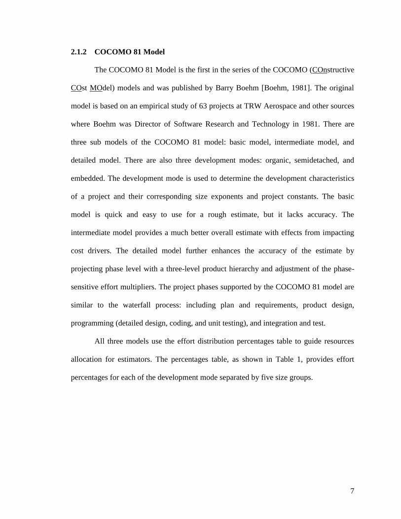
to compute the “weight” of the software. Combined with other factors, effort in person

hours or months is calculated and schedule is produced to map the nine DOD-STD-

2167A phases: System Concept through Operational Test and Evaluation, detail phases

shown in Table 5. TruePlanning®, the commercial suite that contains True S and the

COCOMO II model, produces a staffing distribution that depicts the number of staff

needed by category throughout the project lifecycle, i.e. the number of test engineers or

design engineers needed as the project progresses. Additionally, True S also calculates

support effort in three support phases: maintenance, enhancements, and growth.

Table 5: Lifecycle Phases Supported by True S

DoD-STD-2167A Phases Other Support Phases

True S

System Requirements

Software Requirements

Preliminary Design

Detailed Design

Code/Unit Test

Integration & Test

Hardware/Software Integration

Field Test

System Integration and Test

Maintenance

Enhancement

Growth

Similar to SEER-SEM and SLIM, it is difficult to trace the connection between

application type input and effort distribution guideline as there is little known about the

model or how total effort is distributed to each phase. From the surface, we can only see

the end results, in which a cost schedule is produced according to the engineering phases.

17

2.2 Research Studies on Effort Distribution Estimations

In addition to the mainstream models’ proposed effort distribution guidelines,

some recent studies also focus on effort distribution patterns.

2.2.1 Studies on RUP Activity Distribution

A number of the studies are related to the Rational Unified Process (RUP) for its

clear definitions in project phases and disciplines as well as straightforward guidance on

effort distribution.

The Rational Unified Process [Kruchten, 2003] is an iterative software

development process that is commonly used in modern software projects. The RUP hump

chart, as shown in Figure 2, is famous for setting a general guideline of effort distribution

for the RUP process. The “humps” in the chart represent the amount of effort estimated

for a particular discipline over the four major life cycle phases in RUP. There are six

engineering disciplines: business modeling, requirements, analysis and design,

implementation, test, and deployment. There are also three supporting disciplines:

configuration and change management, project management, and environment.

18

Figure 2: RUP Hump Chart

Over the years, there have been many attempts to validate the RUP hump chart

with sample data sets. A study by Port, Chen, and Kruchten [Port, 2005] illustrates their

experiment that assessed 26 classroom projects that used the MBASE/RUP process and

found that their results do not follow the RUP guideline.

Similarly, Heijstek investigates Rational Unified Process effort distribution based

on 21 industrial software engineering projects [Heijistek, 2008]. In his study, Heijstek

compared the phase effort measured against several other studies and found that his

industrial projects spent less time during elaboration and more during transition. He also

produced visualization of his effort data to compare against the RUP hump chart. He

observed similarities in most major disciplines, but noted discrepancies in supporting

19

disciplines such as configuration and change management and environment. He also

extended his research in modeling the impact of effort distribution on software

engineering process quality and concluded that effort distribution can serve as a predictor

of system quality.

2.2.2 Studies on Effort Distribution Impact Drivers

In addition to studies on RUP, there are also works that investigate the influential

factors that impact effort distribution patterns. These works also use extensive empirical

analyses to back their findings.

Yang et al. [Yang, 2008] conducted a research study on 75 Chinese projects to

investigate affecting factors of variant phase effort distribution. They compared the

overall effort distribution percentages against the COCOMO II effort percentages and

found disagreements between the two in plan/requirement and design phases. They also

performed in-depth analyses on four candidate factors: development lifecycle (waterfall

vs. iterative), development type (new development, re-development, or enhancement),

software size (divided into 6 different size groups), and team size (four different team

size groups).

For each of the candidate factors, Yang et al. compared the effort distribution

between the sub-groups visually and then verified the significance of the differences

using simple ANOVA tests. Their results indicate that factors such as development type,

software size, and team size have visible impacts on effort distribution pattern, and they

can be used as supporting drivers when making resource allocation decisions.

20

Kultur et al conducted a similar study with application domain as an additional

factor in development type and software size [Kultur, 2009]. In their study, they filtered

out 395 ISBSG data points from 4106 software projects, where each data point is given a

clear application domain along with development type (new development, re-

development, or enhancement) and software size. The application domains used in this

research include banking, communications, electricity/gas/water, financial/property/

business services, government, insurance, manufacturing, and public administration.

The researchers compared the overall effort distribution by domains with the

COCOMO II effort percentages, and suggested that some domains follow COCOMO II

distribution whereas others present visible differences. Additionally, they cross-examined

application domains, development types, and software size for each phase in order to

uncover more detailed effort distribution patterns. They applied these distribution

patterns to the sample data sets and calculated MMRE value between use of domain-

specific distribution and no use of domain-specific distribution. Their results indicate

obvious improvements for various domains and phases and therefore call to encourage

the use of domain-specific effort distribution for future analysis. However, unlike Yang’s

analysis, their reports are not enclosed with detail definitions of the application domains

and software process phases, which will need further investigation into the validity of

their results.

21

CHAPTER 3: RESEARCH APPROACH AND METHODOLOGIES

This chapter documents the main approach used to achieve the research goal

including descriptions of various methodologies and techniques for different analyses.

3.1 Research Overview

In order to achieve the research goal of improving the COCOMO II effort

distribution guideline, I began by addressing the most complex hypothesis: the variation

of effort distribution by application domain. Subsequently, I addressed the simpler

hypotheses on variation by project size and personnel capability. Three smaller goals are

defined to accomplish this: 1) determine the domain definitions (or domain breakdown)

to be supported by the improved model; 2) find a sufficient data set; and 3) find solid

evidence of different effort distribution patterns for improved effort distribution

percentages for the COCOMO II model. For the smaller objectives, the following

separated yet correlated studies are conducted:

1) Establish domain breakdown definitions.

2) Select and process subject data set.

3) Analyze data and build model.

Note that these studies are not necessarily done sequentially. For instance, the

tasks of establishing the domain breakdown are generally done in parallel with data

processing tasks so that the right domain breakdown can be generated to cover all the

22

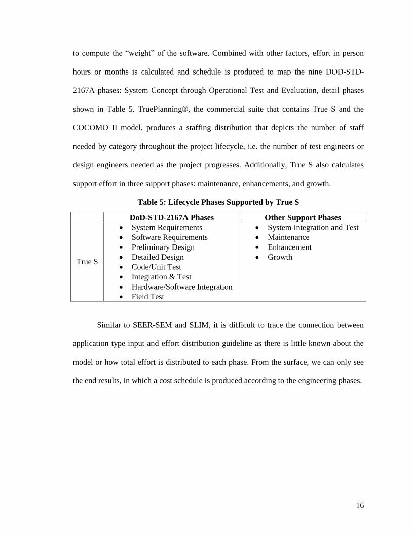
data points. Subsequently, I tested the variation hypotheses for project size and personnel

capability, and found no support for the variation hypotheses. Figure 3 depicts the

relationships between domains, project size, personnel capability, and the subject data set

for this research. It also provides an overall guidance that lists detailed tasks for each

smaller study.

Figure 3: Research Overview

3.2 Effort Distribution Definitions

In order for this research to run smoothly, a unified set of effort distribution

definitions must be established before conducting any analysis. There are two sets of

standard definitions that are considered for this research: development activities defined

in the data dictionary from the data source [DCRC, 2005] and the COCOMO II model

definitions on lifecycle activities and phases. Both sets hold their edge as the favorite for

this research. Data dictionary is used by all the data points and COCOMO II model

23

definition is well-known and widely used by all industry leaders. Still both are not perfect

on their own. Therefore, a merging effort takes place to map the overlapping activities,

namely plan & requirements, architecture & design, code & unit testing, and integration

& qualification tests. The result of this mapping is shown in Table 6. Using this mapping,

the two sets of definitions can be connected to form a unified set that facilitates data

analyses in this research. Note that because the data does not cover any transition

activities, the transition phase from the COCOMO II model is excluded from this

research.

Table 6: Mapping of SRDR Activities to COCOMO II Phases

COCOMO II Phase SRDR Activities

Plan and Requirement Software requirements analysis

Product Design and

Detail Design Software architecture and detailed design

Coding and Unit Testing Coding, unit testing

Integration and testing

Software integration and system/software

integration;

Qualification/Acceptance testing

3.3 Establish Domain Breakdown

Another important set of definitions is the domain breakdown – definitions for the

domains or types that are used as the input of the domain-based effort distribution model.

Establishing such domain breakdown from scratch is extremely challenging. It will

require years of effort summarizing distinctive features and characteristics from many

different software projects with valid domain information. Then, it will need a number of

Delphi discussions among various experts to establish the best definitions. A number of

independent reviews will also take place in order to finalize the definitions. Any of these

24

tasks will take a long time to complete and the results of the new breakdown may arise

from a dissertation of its own.

An alternative and rather simple approach is to research well-established domain

taxonomies and use either an appropriate taxonomy or a combination of several

taxonomies that have enough domain definitions to cover the research data. The

following tasks outline the approach to completing the establishment of the domain

breakdown:

Select the appropriate domain taxonomies.

Understand how these taxonomies describe the domains, i.e. the

dimension that these taxonomies are using to come up with domain

definitions.

Make a master domains list and group the similar domains.

Select those that can be applied to the research data set.

Note that this part of the research is done with researchers from my sponsored

program [AFCAA, 2011], with whom we are building a software cost estimation manual

for the government. In this joint research, we have reviewed a long list of domain

taxonomies and selected the following seven taxonomies that can cover both government

and commercial projects, and are applicable to our data set:

North American Industry Classification System (NAICS)

IBM’s Work-group Taxonomy

Digital’s Industry and Application Taxonomy

MIL-HDBK-881A WBS Standard

25

Reifer’s Application Domains

Putnam’s Breakdown of Application Types by Productivity

McConnell’s Kinds of Software Breakdown

Among these taxonomies, NAICS [NAICS, 2007] is the official taxonomy to

categorize industries based on goods-producing and service-providing functionalities of

businesses. It is a rather high-level categorization, yet does provide a quality perspective

on industry taxonomy. IBM [IBM, 1988] and Digital’s [Digital, 1991] taxonomies focus

primarily on commercial software projects from the perspectives of both industry and

system capability. Both provide comprehensive guideline in determining the software

project’s domain using cross references on its industry and application characteristics.

The Mil-HDBK-881A standard [DoD HDBK, 2005] is used by the US government to

provide detailed WBS guideline for different military systems. The first two levels of the

WBS structure provide the description of the system’s overall operating environment and

high-level functionalities, thus giving us a breakdown in terms of domain knowledge.

This standard is especially useful because it provides a broad view of government

projects which we have not received explicitly from the previous three taxonomies. Both

Putnam’s [Putnam, 1976] and McConnell’s [McConnell, 2006] application type

breakdowns are based on productivity range and size divisions. This tells us that

application types may contain certain software product characteristics that have direct

relationships with productivity. Confirming this approach, Reifer [Reifer, 1990] also

indicates the importance of productivity in relation to application domains, which he

summarized from real-world data points to cover a wide range of software systems

26

ranging from government to commercial projects. The following table shows a

comparison between our subject taxonomies.

Table 7: Comparisons of Existing Domain Taxonomies

Taxonomy

Name

Number of

Domains

Defined

Breakdown Rationale Considered

Size Effect

Considered

Productivity

Effect

NAICS 10 industries

domains.

Categorizing goods-

producing industries and

service-providing industries.

No No

IBM 46 work groups;

8 business

functions

(across-industry

application

domains).

Use work groups as

horizontal perspective and

business functions as

vertical perspective to pin-

point a software project.

No No

Digital 18 industry

sectors;

18 application

domains.

Combines domain

characteristics with industry

definitions. No No

Reifer’s 12 application

domains.

Summarized from 500 data

points based on project size

and productivity range.

Yes Yes

Mil-881A 8 system types. Provide WBS for each

system type. Level 2 in

WBS describes the

application features.

No No

Putnam’s 11 application

types.

Using productivity range to

categorize application types. Yes Yes

McConnell’s 13 kinds of

Software.

Adopted from Putnam’s

application types, refined

the taxonomy with software

size groups.

Yes Yes

After careful review and study of these taxonomies, we have also come to a

common understanding that there are two main dimensions we can look to determine

domains — platform and capability. Platform describes the operating environment in

27

which the software system will reside. It provides the key constraints of the software

system in terms of physical space, power supplies, data storage, computing flexibility, etc.

Capability outlines the intended operations of the software system and indicates the

requirements of the development team in terms of domain expertise. Capability may also

suggest the difficulties of the software project given nominal personnel rating of the

development team.

With a prepared master list of domain categories and the notion to use both

platform and capability dimensions, we put together our domain breakdown in terms of

operating environment (8) and application domains (21). Each can describe a software

project on its own terms. Operating environment defines the platform and product

constraint of the software system whereas application domains focus on the common

functionality descriptions of the software system. We can use them together or separately

as they do not interfere with each other. A detailed breakdown of the operating

environment and application domains is documented in Appendix A.

Although this initial version of the domain breakdown is sufficient to differentiate

software project, we can do more. We have not applied productivity ratings for this

breakdown. We have analyzed further breakdown using productivity rate. Upon further

comparisons of these taxonomies and data analysis, a proposal was filed for a more

simplified domain breakdown.

In this newer version of the domain breakdown, the 21 application domains are

grouped by its productivity range. We call this new group “productivity types” or “PT”.

Detailed definitions of productivity types can also be found in Appendix A. The eight

28

operating environments are essentially the same as the previous version but split into 10

operating environments. The following table shows a mapping between our application

domains and the productivity types. Note that there are some application domains that

can be mapped to more than one productivity type. This is because the application

domains are covering more than one major capability that spreads across more than one

productivity range.

Table 8: Productivity Types to Application Domain Mapping

Productivity Types Application Domains

Sensor Control and Signal Processing (SCP) Sensor Control and Processing

Vehicle Control (VC) Executive

Spacecraft Bus

Real Time Embedded (RTE) Communication

Controls and Displays

Mission Planning

Vehicle Payload (VP) Weapons Delivery and Control

Spacecraft Payload

Mission Processing (MP) Mission Management

Mission Planning

Command & Control (C&C) Command & Control

System Software (SYS) Infrastructure or Middleware

Information Assurance

Maintenance & Diagnostics

Telecommunications (TEL) Communication

Infrastructure or Middleware

Process Control (PC) Process Control

Scientific Systems (SCI) Scientific Systems

Simulation and Modeling

Training (TRN) Training

Test Software (TST) Test and Evaluation

Software Tools (TUL) Tools and Tool Systems

Business Systems (BIS) Business

Internet

In this research, both application domains and productivity types are candidates

for support by the domain-based effort distribution model. Both breakdowns will be

29

thoroughly analyzed, compared, and contrasted according to the analysis procedure

documented in Section 3.5.

3.4 Select and Process Subject Data

The data is primarily project data from government funded programs collected

through Department of Defense’s Software Resource Data Report [DCRC, 2005]. Each

data point consists of the following sets of information: a set of effort values such as

person hours for requirements to qualification testing activities; a set of sizing

measurements such as new size, modified size, unmodified size, etc.; and a set of project

specific parameters such as maturity level, staffing, requirement volatility, etc.

Additionally, each data point is attached with its own refined data dictionary. Our

program sponsor, the Air Force Data Analysis Agency, sanitized the data set by removing

all project identity information and helped us define the application domains and

operating environment for these projects.

The original data sets are not perfect: missing data points, unrealistic data values,

and ambiguous data definitions are common in our data sets. As a result, normalizing and

cleansing of data points is needed for the data analyses. First, records with significant

defects need to be located and eliminated from the subject data set: defects such as 1)

missing important effort or size data; 2) missing data definitions on important effort or

size data, i.e. no definition indicating whether size is measured in logical or physical lines

of code; and 3) duplicated records. Second, abnormal and untrustworthy data patterns

need to be reviewed and handled in the subject data set: patterns, which are made of huge

30

size with little effort or vice versa. For example, there is a record with one million lines

of code, produced in 3 to 4 person months with all lines of code as new size. After

removing all problematic records, two additional tasks need to be performed: 1) backfill

missing effort of remaining activities and 2) test for overall normality of the data set.

There are two approaches to backfilling effort data. The first uses simple averages

of the existing records to calculate the missing values. The second uses matrix

factorization to approximate missing values [Au Yeung; Lee, 2001]. After a few attempts,

the first approach proved to be less effective than the second and produced with large

margins of errors. Therefore, the second approach, matrix factorization, is the best choice.

In matrix factorization, we start with two random matrices, W and H, whose dot product

equals the dimension of our data set, X0. By iteratively adjusting values of W and H, we

can find the closest approximation such that W x H X, where X is an approximation of

X0. This process typically sets a maximum iteration number to be at least 5,000 to 10,000

in case W x H never reach close enough to X0. This algorithm is applied to three subsets:

a subset missing 2 out of 5 activities at most; a subset missing 3 out of 5 activities, and a

subset missing 4 out of 5 activities. Setting approximation exit margin to 0.001 and run

for 10,000 iterations, backfilled data with very small margin of errors is produced,

usually with 10% of the original (when comparing against existing data values). Figure 4

shows an example of the resulting data.

31

Figure 4: Example Backfilled Data Set

Notice that few records are observed with huge margin of errors. This typically

results when a value for one activity is extremely small, while the values for other

activities are relatively large. Although this discrepancy seems harmful to the data

process results, a low number among a large collection of data points lowers the

possibility of entering large error. On the positive side, this discrepancy can help us

identify possible outliers in our data set if we experience situations when we need to

analyze outlier effects.

The last step is to run basic normality tests on the data set. These tests are crucial

because they validate the initial assumption which states that all of the data points are

independent from each other and therefore normally distributed. The initial assumption is

made because there is no known source information or detailed background information

for all projects in the data set. We can only assume that they are not correlated in any way,

and are thus independent from each other.

Since the subject data fields are effort data, it is only necessary to run the tests on

this data. Both histogram and Q-Q diagrams [Blom, 1958; Upton, 1996] are produced to

visualize the distribution. Several normal distribution tests such as Shapiro-Wilk test

32

[Shapiro, 1965], Kolmogorov-Smirnov test [Stephens, 1974], and Pearson’s Chi-square

test [Pearson, 1901] are performed to check the distribution normality and to determine

whether the data set is good for analysis.

In addition to checking, eliminating, and backfilling, calculating the equivalent

lines of code, converting person-hours to person months, summing up the schedule in

calendar months, and calculating the equivalent personnel ratings for each project are

also taken place as part of the data processing.

3.5 Analyze Data and Build Model

The final piece of this research focuses on answering the central question and

building an alternative model to the current COCOMO II Waterfall effort distribution

guideline. There are two major steps in this part of the study: 1) calculate and analyze

effort distribution patterns and 2) build and implement the model. These two steps are

described in full detail in the following sub sections.

3.5.1 Analyze Effort Distribution Patterns

In studying effort distribution patterns, two rounds of analyses are conducted. In

the first round, we analyze the initial version of domain breakdown with 21 application

domains. In the second round, we analyze the refined version of 14 productivity types.

Each round follows the same analysis steps, as described below. The results from each

round will be analyzed and compared. Based on the comparison, one domain breakdown

33

is determined as the domain information set that will be supported by the new effort

distribution model.

Effort Distribution Percentages:

From the data processing results, effort percentages by activity groups can be

calculated for each project. Percentage means of each domain can also be found by

grouping the records. By looking at the trend lines, simple line graph can help us

visualize the distribution patterns and find interesting points. Although the plots may

indicate large gaps of percentage means between domains, the evidence will not be solid

enough to prove the difference significant. Statistical proofs are also needed. Single

factor of variance (ANOVA) can be used for this proof. We line up all the data points in

each domain and use the ANOVA test to determine whether the variance between

domains is caused by mere noise or truly represents differences. The null hypothesis for

this test is that all domains will have the same distribution percentage means for each

activity. The alternative hypothesis is that domains have different percentage means,

which is the desired result because this will prove that domains have their effect over


Once the ANOVA tests conclude, a subsequent test must be performed to find out

if the domains’ percentage means are different from COCOMO II Waterfall effort

distribution guideline’s percentage means. This is important because if the domains

percentage means are no different from the current COCOMO II Waterfall model, then

this research will have no ground in enhancing the COCOMO II model in effort

distribution. Table 9 shows the COCOMO II Waterfall effort distribution percentages.

34

Table 9: COCOMO II Waterfall Effort Distribution Percentages

Phase/Activity Effort %

Plan and Requirement 6.5

Product Architecture & Design 39.3

Code and Unit Testing 30.8

Integration and Qualification Testing 23.4

Note that COCOMO II model’s percentage means have been divided by 1.07

because the original COCOMO II model’s percentage means sum up to 107% of the full

effort distribution.

In order to find out if there are any differences, the independent one-sample t-test

[O’Connor, 2003] is used. The formula for the t-test is shown as follows:

√

(EQ. 4)

Statistic t in the above formula is to test the null hypothesis that sample average

is equal to a specific value , where s is the standard deviation and n is the sample size.

In our case, would be the COCOMO II model’s effort distribution averages and is a

domain’s distribution percentage average for each activity group. The rejection of the

null hypothesis in each effort activity can provide a conclusion that the domain average

does not agree with the COCOMO II model’s effort distribution averages. Such an ideal

result may indicate that the current COCOMO II model’s effort distribution percentages

are not sufficient for accurate estimation for effort allocation and thus it is necessary to

find an improvement.

In both ANOVA and t-tests, 90% significance level to accept or reject the null

hypothesis is used because the data is from real world projects and the noise level is

35

rather high. If the tests indicate a mix between rejections and acceptances, a consensus of

the results can be used to determine a final call on rejection or acceptance.

3.5.1.1 Comparison of Application Domains and Productivity Types

The final step in data analysis is a comparison analysis of the results from

application domains and productivity types. The purpose of this comparison is to evaluate

the applicability of these domain breakdowns as the main domain definition set to be

supported by the domain-based effort distribution model.

In this comparison, general effort distribution patterns are compared to find out

which breakdown provides stronger trends that show more differences between domains

or types. Similarly, the statistical test results are analyzed for the same reason. Lastly, the

characteristics and behaviors of application domains and productivity types are analyzed

to compare their identifiability, availability, and supportability.

3.5.1.2 Project Size

To study project size, data points are divided into different size groups. Effort

distribution patterns for each size group are produced and analyzed. The goal of this

analysis is to find possible trends within a domain or type that is differentiated by project

size. Since size is a direct influential driver of effort in most estimation models, a direct

and simple relationship that proportionally increases or decreases project size and effort

percentages is expected. Again, statistical tests are necessary if such a trend is found to

prove its variance significance level.

36

The challenge of this analysis is the division of size groups. Some domains/types

may not have enough total data points to be divided into size groups and some

domains/types may not have enough data points in one or more size groups. Either case

can inhibit determination of the best size driver on effort distribution patterns.

3.5.1.3 Personnel Capability

For the personnel rating, the SRDR data supplies three personnel experience

percentages: Highly Experienced, Nominally Experienced, and Inexperienced/Entry

Level. The experience level is evaluated by the years of experience the staff has worked

on software development as well as the years of experience the staff has worked within

the mission discipline or project domain. Given these percentages, an overall personnel

rating can be calculated using the three COCOMO II personnel rating driver values:

Application Experience (APEX), Platform Experience (PLEX), and Language and Tool

Experience (LTEX). The following formula is used to calculate personnel ratings for

each data point. Table 10 shows the driver values of APEX, PLEX, and LTEX of

different experience levels.

( ) ( )

( ) (EQ.5)

where

Table 10: Personnel Rating Driver Values

Driver Names High (~3 years) Nominal (~1 year) Low (~6 months)

APEX 0.81 1.00 1.10

PLEX 0.91 1.00 1.09

LTEX 0.91 1.00 1.09

PEXP 0.67 1.00 1.30

37

Using the calculated personnel ratings, data points can be plotted as personnel

ratings versus effort percentages for each activity group in a domain/type. Trends can be

observed from these plots if increases in personnel ratings results in decreasing in effort

percentages or vice versa. For simplicity, the end result for the personnel rating will be

kept in linear adjustment factor (at least as close to linear as possible).

3.5.2 Build Domain-based Effort Distribution Model

From the analyses of effort distribution patterns by application domains and

productivity types, project size, and personnel ratings, the variations by size and

personnel ratings were negligible, and the effort distribution model was based on domain

variation. A set of effort distribution percentages by application domains, and the domain

definitions set to be used in the model were collected and readied to build the domain-

based effort distribution model.

The key guideline for designing the model is that it has to be similar to the

current COCOMO II model design. Both Waterfall and MBASE effort distribution

models use average percentage tables in conjunction with size as partial influential factor.

This compatibility must be established in the new model. Additionally, procedures for

using the model should not be more complicated than what are currently provided by the

COCOMO II model. That is, without any more instruction than to input all the

COCOMO II drivers and necessary information, the model should produce the effort

distribution guideline automatically as part of the COCOMO II estimates. The only

additional input required may be the domain information. Comparison of the effort

38

distribution guideline produced by the COCOMO II Waterfall model and the new model

can also be added as a new feature to make this model more useful.

When the design of the model is complete, it is important to provide an

implementation instance of the model to demonstrate its features. In order to accomplish

this, an instance of the COCOMO II model must be selected with source code as the

implementation environment for the new model. After the new model implementation is

complete, a comparison of results between COCOMO II Waterfall model and the

domain-based effort distribution model must be conducted to test the new model’s

performance.

39

CHAPTER 4: DATA ANALYSES AND RESULTS

This chapter summarizes the key data analyses and their results conducted in

building the domain-based effort distribution model and testing the domain-variability

hypothesis.

Section 4.1 provides an overview of the data selection and normalization results

that defines the baseline data sets for the data analyses. Section 4.2 and 4.3 reports the

data analyses performed on the data sets grouped by application domains and

productivity types respectively. Section 4.4 reviews the analyses results and compares the

pros and cons between application domains and productivity types. Finally, Section 4.5

discusses the conclusions drawn from the data analyses.

4.1 Summary of Data Selection and Normalization

Data selection and normalization are completed before most data analyses are

started. A set of 1,023 project data points was collected by our data source and research

sponsor, the AFCAA, and given to us for initiation of the data selection and

normalization process. As discussed in Section 3.4, simple and straight forward browsing

through data points helped us eliminate most defective (missing effort, size, or important

data definitions such as counting method or domain information) and duplicated data

points. Further analysis of abnormal data patterns also identified and removed more than

40

a dozen data points. A total of 530 records remains in our subject data set to begin the

effort distribution analysis.

Although these 530 records are completed with total effort, size, and other

important attributes, they need further processing to ensure sufficient phase effort data.

Some records do not have all the phase effort distribution data that we need for the effort

distribution analysis. Having eliminated those without phase effort distribution data, we

are left with 345 total data points that we can work with. The table below illustrates the

overall data selection and normalization progress.

Table 11: Data Selection and Normalization Progress

Data Set Record Count

Action Results

1023 Browsing through data records: looks for defective and duplicated data points.

Eliminated 479 defective and duplicated data points.

544 Look for abnormal or weird patterns.

Eliminated 14 data points.

530 Remove records with insufficient effort distribution data.

Eliminated 185 data points.

345 Divide data set by the number of missing phase effort fields.

Ready to create 3 sub sets, namely “missing 2”, “missing 1”, and “perfect” sets. Missing 4 and Missing 3 are ignored because they still miss too much information to be persuasive.

257 Backfilled the two missing phase effort fields.

Created “Missing 2” set.

221 Backfilled the only one missing phase effort field.

Created “Missing 1” set.

135 None. Created “Perfect” set.

“Missing 2” and “Missing 1” sets were created as comparison sets against the

“Perfect” set in order to 1) increase the number of data points in the sample data set, and

2) outlook the data pattern as more data points become available in the future. The

41

method for backfilling is very effective in predicting continuous and correlated data

patterns such as the effort distribution patterns we are focusing on. Therefore, the

resulting data sets are sufficient for our data analysis. Since there is little difference

between the “Missing 2” and “Missing 1” sets, we have used only the “Missing 2” set.

Two copies are created for each of the “Missing 2” and “Perfect” sets. One copy

is grouped by Application Domains, and the other copy is grouped by Productivity Types.

We are now ready for our main data analyses.

4.2 Data Analysis of Domain Information

4.2.1 Application Domains

The following table is the records count by application domains. Note the

highlighted rows are the domains with sufficient number of data points in all three sub

sets. The threshold for sufficient data points count is five.

42

Table 12: Research Data Records Count - Application Domains

Research Data Records Count Application Domains Missing 2 Missing 1 Perfect Set

Business Systems 6 6 5 Command & Control 31 25 15 Communications 51 47 32 Controls & Displays 10 10 5 Executive 3 3 3 Information Assurance 1 1 1 Infrastructure or Middleware 8 3 1 Maintenance & Diagnostics 3 1 1 Mission Management 28 26 19 Mission Planning 14 13 10 Process Control 4 4 0 Scientific Systems 3 3 3 Sensor Control and Processing 27 22 10 Simulation & Modeling 19 18 11 Spacecraft BUS 9 9 5 Spacecraft Payload 2 2 0 Test & Evaluation 2 1 1 Tool & Tool Systems 7 7 2 Training 1 1 0 Weapons Delivery and Control 28 19 10 Total 257 221 135

Overall Effort Distribution Patterns:

For each of the highlighted Application Domains, average effort percentages of

each activity group are calculated from the data records and then plotted to visualize the

effort distribution pattern. Table 13 and Figure 5 illustrate the “Perfect” set whereas

Table 14 and Figure 6 illustrate the “Missing 2” set.

43

Table 13: Average Effort Percentages - Perfect Set by Application Domains

Average Effort Percentages – Perfect Set Domain REQ ARCH CUT INT Business Biz 20.98% 22.55% 24.96% 31.51% Command & Control CC 21.04% 22.56% 33.73% 22.66% Communications Comm 14.95% 30.88% 28.54% 25.62% Control & Display CD 14.72% 34.80% 24.39% 26.09% Mission Management MM 15.40% 17.78% 28.63% 38.20% Mission Planning MP 17.63% 12.45% 44.32% 25.60% Sensors Control and Processing Sen 7.78% 45.74% 22.29% 24.19% Simulation Sim 10.71% 39.11% 30.80% 19.38% Spacecraft Bus SpBus 33.04% 20.66% 30.00% 16.30% Weapons Delivery and Control Weapons 11.50% 17.39% 29.82% 41.29%

Figure 5: Effort Distribution Pattern - Perfect set by Application Domains

Among the average effort percentages, it is clear that none of the application

domains produce a similar trend as indicated by the COCOMO II averages, which are 6.5%

0.00%

5.00%

10.00%

15.00%

20.00%

25.00%

30.00%

35.00%

40.00%

45.00%

50.00%

Requirement Arch&Design Code&Unit Test Integration & QT

Pe

rce

nta

ges

Average Effort Percentages Distribution

Biz

CC

Comm

CD

MM

MP

Sen

Sim

SpBus

Weapons

COCOMO II

44

for Requirements & Planning, about 40% for Architecture & Design, about 30% for Code

& Unit Testing, and roughly 23.5% for Integration & Qualification Testing. The closest

application domain to the COCOMO II averages is Simulation, which suggests more time

should be dedicated to Requirements & Planning, while less time should be dedicated

toIntegration & Qualification Testing. All other application domains seem to request a

significant increase in time for Requirements & Planning, except Sensors Control and

Process which seems to allocate most of its time to Architecture & Design. Since most

application domains spend more time on Requirements & Planning, most of them spend

less on Architecture & Design. A few application domains show huge differences for

Code & Unit Testing. Only Mission Planning seems to allocate a significant amount of

time to Code & Unit Testing, perhaps because it tends to do less architecting (only

12.45%). Sensor Control and Processing, on the other hand, spends less time on coding

and unit testing due to more effort in designing the system. Overall, the gap between the

minimum and the maximum average effort percentages for each activity group is

significant, and the average percentages from the application domains are evenly spread

across these gaps, which will be reflected in testing the hypothesis. For the domains with

sufficient data, the domain-specific effort distributions are better than the COCOMO II

distributions, although this also needs statistical validation, which is explored next.

45

Table 14: Average Effort Percentages - Missing 2 Set by Application Domains

Average Effort Percentages – Missing 2 Domain REQ ARCH CUT INT Business Biz 18.51% 23.64% 27.85% 30.00% Command & Control CC 19.41% 23.70% 34.59% 22.31% Communications Comm 14.97% 27.85% 27.89% 29.28% Control & Display CD 14.67% 26.66% 27.72% 30.95% Mission Management MM 16.59% 17.60% 25.74% 40.07% Mission Planning MP 14.41% 16.42% 43.47% 25.69% Sensors Control and Processing Sen 7.75% 31.84% 25.32% 35.09% Simulation Sim 13.73% 29.09% 30.33% 26.85% Spacecraft Bus SpBus 36.38% 17.23% 27.90% 18.50% Weapons Delivery and Control Weapons 11.73% 17.79% 28.97% 41.51%

Figure 6: Effort Distribution Pattern - Missing 2 Set by Application Domains

0.00%

5.00%

10.00%

15.00%

20.00%

25.00%

30.00%

35.00%

40.00%

45.00%

50.00%


Pe

rce

nta

ges


Biz

CC

Comm

CD

MM

MP

Sen

Sim

SpBus

Weapons

COCOMO II

46

Similar to what has already been observed from the “Perfect” set, data points

from the “Missing 2” set produce effort distribution patterns that show wide gaps

between the minimum and the maximum for each activity group, while scattering average

percentages from application domains somewhat evenly. One thing to notice is that for

Requirements & Planning, Spacecraft Bus pushed the maximum to over 35% while most

of the other application domains stayed below 20%. This could have resulted because the

Spacecraft Bus domain needs to satisfy the requirements for a family of spacecraft

systems.

ANOVA and T-Test:

Although the plot shows obvious differences between the distribution patterns of

application domains, more mathematical evidence is needed to fully support use of the

domain-based effort distribution patterns. Using ANOVA to test the significant level of

the differences between application domains can help us confirm the hypothesis. We

need to reject the null hypothesis that all application domains will produce the same

effort distribution pattern. Table 15 lays out the results for both the “Perfect” and

“Missing 2” set. F and P-value are calculated for each activity group to evaluate whether

the variances between application domains are produced by noise or patterns that dictate

the differences. With strong rejections for every activity group, the ANOVA results favor

the hypothesis and ensure the differences between different application domains are not

merely coincidental.

47

Table 15: ANOVA Results - Application Domains

Activity Group

“Perfect” Data Set “Missing 2” Data Set

F P-

Value Results F P-

Value Results

Plan & Requirements

2.9461 0.0035 Reject 7.2908 0.0000 Reject

Architecture & Design

4.5656 0.0000 Reject 3.5347 0.0004 Reject

Code & Unit Testing

2.1018 0.0350 Reject 3.3470 0.0007 Reject

Integration and Qualification Testing

3.7787 0.0003 Reject 7.2467 0.0000 Reject

Given strong support from the ANOVA results for the hypothesis, the T-Test

results also provide encouraging evidence that domain-based effort distribution is a good

alternative to the conventional COCOMO Averages. As shown in Table 16, most

application domains are far from the COCOMO average in Plan & Requirements and

Architecture & Design activity groups, and are somewhat apart in Integration &

Qualification Testing. However, only few application domains disagree with the

COCOMO average in Code & Unit Testing. This may be because most of COCOMO II’s

calibration data points are completed with Code & Unit Testing effort data, while lacking

quality support from other activity groups, particularly in Plan & Requirement and

Architecture & Design. In summary, the results favor three out of the four activity groups;

and therefore, add support for using domain-based effort distribution patterns.

48

Table 16: T-Test Results - Application Domains

Activity Group

COCOMO Averages


Plan & Requirements

6.5% All domains reject except Control and

Display, Sensor Control, and

Simulation domains.

All domains reject except Sensor Control.


39.3% All domains reject except Control and

Display, Sensor Control, and

Simulation domains.

All domains reject except Control and Display.

Code & Unit Testing

30.8% Only Mission Planning rejects.

Communication, Mission Management, Mission

Planning, and Sensor Control reject, other six domains do

not.


23.4% Only Mission Management,

Spacecraft Bus, and Weapon Delivery

domain reject.

Communications, Mission Management, Sensor

Control, Spacecraft Bus, and Weapons Delivery domains reject; other five domains do

not.

4.2.2 Productivity Types

The following table illustrates the records count by productivity types. Note the

highlighted rows are the types with a sufficient number of data points in all three sub sets.

Again, the threshold count of sufficient data points is five.

49

Table 17: Research Data Records Count - Productivity Types

Research Data Records Count Productivity Types Missing 2 Missing 1 Perfect Set

C&C 8 3 0 ISM 14 14 6 MP 28 23 14 PC 7 6 3 PLN 10 9 7 RTE 57 49 33 SCI 22 21 16 SCP 35 28 12 SYS 27 23 15 TEL 4 4 4 TRN 4 4 3 TST 2 2 1 TUL 4 3 2 VC 26 25 15 VP 9 7 4 Total 257 221 135

Overall Effort Distribution Patterns:

For each of the highlighted Productivity Types, average effort percentages of each

activity group are calculated from the data records and then plotted to visualize the effort

distribution pattern. Table 13 and Figure 5 illustrate the “Perfect” set whereas Table 14

and Figure 6 illustrate the “Missing 2” set.

50

Table 18: Average Effort Percentages - Perfect Set by Productivity Types

Average Effort Percentages – Perfect Set Productivity Type Requirement Arch&Design Code&Unit Test Integration & QT ISM 11.56% 27.82% 35.63% 24.99% MP 20.56% 15.75% 28.89% 34.80% PLN 16.22% 12.27% 50.78% 20.73% RTE 15.47% 26.65% 26.71% 31.17% SCI 7.38% 39.90% 32.05% 20.67% SCP 10.80% 45.20% 20.34% 23.66% SYS 17.61% 21.10% 28.75% 32.54% VC 18.47% 23.60% 31.32% 26.61%

Figure 7: Effort Distribution Pattern - Perfect set by Productivity Types

The average effort percentages are very similar to those from application domains.

This is expected since several Productivity Types are essentially the same as their

application domains counterparts (for instance, SCI = Scientific and Simulation Systems,

PLN = Systems for Planning and Support Activities, and SCP = Sensor Control and

0.00%

10.00%

20.00%

30.00%

40.00%

50.00%

60.00%


Pe

rce

nta

ges


ISM

MP

PLN

RTE

SCI

SCP

SYS

VC

COCOMO II

51

Processing). Again, the gaps between minimum and maximum average percentages is

easy to spot in the plot, and average percentages from Productivity Types are spreading

across these ranges following the same even fashion.

Table 19: Average Effort Percentages - Missing 2 Set by Productivity Types

Average Effort Percentages – Missing 2 Productivity Type Requirement Arch&Design Code&Unit Test Integration & QT ISM 12.34% 25.32% 32.81% 29.53% MP 22.43% 15.06% 26.11% 36.40% PLN 14.99% 14.15% 49.23% 21.62% RTE 15.43% 24.02% 28.84% 31.70% SCI 7.40% 34.98% 30.47% 27.15% SCP 12.50% 29.07% 24.11% 34.32% SYS 15.74% 20.87% 32.61% 30.79% VC 18.02% 21.36% 30.02% 30.59%

Figure 8: Effort Distribution Pattern - Missing 2 Set by Productivity Types

0.00%

10.00%

20.00%

30.00%

40.00%

50.00%

60.00%


Pe

rce

nta

ges


ISM

MP

PLN

RTE

SCI

SCP

SYS

VC

COCOMO II

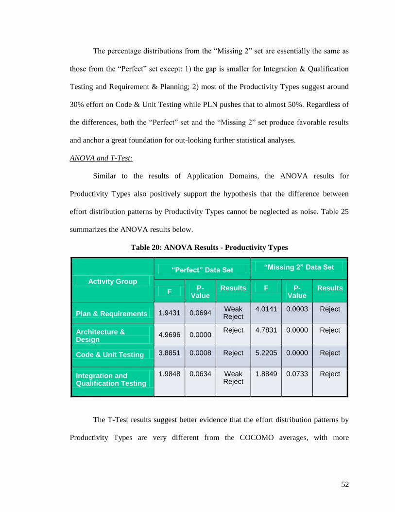
52

The percentage distributions from the “Missing 2” set are essentially the same as

those from the “Perfect” set except: 1) the gap is smaller for Integration & Qualification

Testing and Requirement & Planning; 2) most of the Productivity Types suggest around

30% effort on Code & Unit Testing while PLN pushes that to almost 50%. Regardless of

the differences, both the “Perfect” set and the “Missing 2” set produce favorable results

and anchor a great foundation for out-looking further statistical analyses.

ANOVA and T-Test:

Similar to the results of Application Domains, the ANOVA results for

Productivity Types also positively support the hypothesis that the difference between

effort distribution patterns by Productivity Types cannot be neglected as noise. Table 25

summarizes the ANOVA results below.

Table 20: ANOVA Results - Productivity Types

Activity Group


F P-

Value Results F P-

Value Results

Plan & Requirements 1.9431 0.0694 Weak Reject

4.0141 0.0003 Reject


4.9696 0.0000 Reject 4.7831 0.0000 Reject

Code & Unit Testing 3.8851 0.0008 Reject 5.2205 0.0000 Reject


1.9848 0.0634 Weak Reject

1.8849 0.0733 Reject

The T-Test results suggest better evidence that the effort distribution patterns by

Productivity Types are very different from the COCOMO averages, with more

53

disagreements in the Code & Unit Testing activity group. These disagreements provide

strong support for using productivity types to further enhance the COCOMO II model in

term of effort distribution.

Table 21: T-Test Results - Productivity Types

Activity Group

COCOMO Averages


Plan & Requirements

6.5% All types reject except ISM, SCI, and SCP.

All types reject except SCI.


39.3% All types reject except SCI and SCP.

All types reject except SCI.

Code & Unit Testing

30.8% Only PLN, RTE, and SCP reject.

Only MP, PLN, and SCP reject.


23.4% Only MP, RTE, and SYS reject.

All types reject except PLN and

SCI.

4.3 Data Analysis of Project Size


Since the data includes other possible sources of variation in effort distribution,

such as size, a study on project size was performed to provide a further in-depth look at

the effort distribution by application domains. As discussed earlier in Chapter 3, data

from each application domain is divided into size groups (providing at least five data

54

points for each size group). Using the average effort percentage from each size group, we

can observe possible effects of size upon the effort distribution patterns. In this study,

three size groups are drawn to divide application domains: 0 to 10 KSLOCs, 10 to 32

KSLOCs, and 32 plus KSLOCs. ANOVA is also performed on each domain where 90%

confidence level is used. Using the ANOVA will help measuring the variability strength

of project size on effort distribution patterns, and compare this strength level against that

resulting from application domains. The following tables show the project size analysis

results for Communication and Mission Management application domains for the

“Perfect” set.

Table 22: Effort Distribution by Size Groups – Communication (Perfect)

Size Group (KSLOC) Count REQ ARCH CODE INT&QT

0 to 10 6 10.7% 50.5% 17.3% 21.5%

10 to 36 12 18.6% 25.2% 31.1% 25.1%

36 + 14 13.7% 27.4% 31.1% 27.8%

ANOVA Results

F 1.364 6.993 4.668 0.582

P-Value 0.272 0.003 0.017 0.565

Result Can’t Reject Reject Reject Can’t Reject

55

Figure 9: Effort Distribution by Size Groups – Communication (Perfect)

Table 23: Effort Distribution by Size Groups - Mission Management (Perfect)


0 to 10 6 16.7% 23.4% 27.1% 32.9%

10 to 36 6 15.5% 14.8% 26.2% 43.5%

36 + 7 14.2% 15.6% 32.0% 38.2%

ANOVA Results

F 0.067 1.071 0.510 0.913

P-Value 0.935 0.366 0.610 0.421

Result Can’t Reject Can’t Reject Can’t Reject Can’t Reject

0.0%

10.0%

20.0%

30.0%

40.0%

50.0%

60.0%

REQ ARCH CODE INT&QT

Ave

rage

Eff

ort

Pe

rce

nta

ges

Effort Distribution by Size Groups - Communication

0 to 10

10 to 36

36 +

56

Figure 10: Effort Distribution by Size Groups - Mission Management (Perfect)

In addition to the two application domains from the “Perfect” set, Command &

Control and Sensor Control & Process application domains from the “Missing 2” set are

also analyzed with the same size groups. Note that no duplicated analysis is done for

Communication and Mission Management domains even though there are enough data

points for those domains in the “Missing 2” set. Results from the “Perfect” set will be

used for those two domains. The following tables and figures provide the results from

those two application domains.

0.0%

5.0%

10.0%

15.0%

20.0%

25.0%

30.0%

35.0%

40.0%

45.0%

50.0%


Ave

rage

Eff

ort

Pe

rce

nta

ges

Effort Distribution by Size Groups - Mission Management

0 to 10

10 to 36

36 +

57

Table 24: Effort Distribution by Size Groups – Command & Control (Missing 2)


0 to 10 6 26.1% 23.2% 28.6% 22.0%

10 to 36 5 15.3% 20.6% 38.6% 25.5%

36 + 20 18.4% 24.6% 35.4% 21.6%

ANOVA Results

F 1.221 0.193 0.973 0.232

P-Value 0.310 0.825 0.390 0.795

Result Can’t Reject Can’t Reject Can’t Reject Can’t Reject

Figure 11: Effort Distribution by Size Groups – Command & Control (Missing 2)

Table 25: Effort Distribution by Size Groups - Sensor Control (Missing 2)


0 to 10 7 9.8% 45.8% 14.6% 29.8%

10 to 36 15 6.6% 28.1% 29.1% 36.2%

36 + 5 8.2% 23.6% 29.0% 39.2%

ANOVA Results

F 0.449 3.258 3.861 0.649

P-Value 0.643 0.056 0.035 0.532

Result Can’t Reject Weak Reject Reject Can’t Reject

0.0%

5.0%

10.0%

15.0%

20.0%

25.0%

30.0%

35.0%

40.0%

45.0%


Ave

rage

Eff

ort

Pe

rce

nta

ges

Effort Distribution by Size Groups - Command and Control

0 to 10

10 to 36

36 +

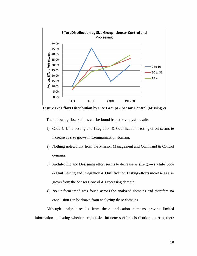
58

Figure 12: Effort Distribution by Size Groups - Sensor Control (Missing 2)

The following observations can be found from the analysis results:

1) Code & Unit Testing and Integration & Qualification Testing effort seems to

increase as size grows in Communication domain.

2) Nothing noteworthy from the Mission Management and Command & Control

domains.

3) Architecting and Designing effort seems to decrease as size grows while Code

& Unit Testing and Integration & Qualification Testing efforts increase as size

grows from the Sensor Control & Processing domain.

4) No uniform trend was found across the analyzed domains and therefore no

conclusion can be drawn from analyzing these domains.

Although analysis results from these application domains provide limited

information indicating whether project size influences effort distribution patterns, there

0.0%

5.0%

10.0%

15.0%

20.0%

25.0%

30.0%

35.0%

40.0%

45.0%

50.0%


Ave

rage

Eff

ort

Pe

rce

nta

ges

Effort Distribution by Size Group - Sensor Control and Processing

0 to 10

10 to 36

36 +

59

are a fair number of other application domains that have not been analyzed. The main

reason for the absence of analysis of other application domains is that there are not

enough data points to divide the domain into size groups. There are two scenarios in

which application domain is dropped due to lack of data points:

1) The overall data points are below the minimum threshold of 15 data points (5

for each size group).

2) There are not enough data points for one or more size groups. For instance,

Command and Control has 15 data points, but there are only 2 data points

with a size less than 10 KSLOCs.

There were attempts to bypass the second scenario by using different divisions of

size groups, but none of these attempts were successful in providing more application

domains to analyze. The current division is a better choice than most of the other

divisions.


The same project size analysis is done for the productivity types. Size groups are

divided as 0 to 10 KSLOCs, 10 to 36 KSLOCs, and 36 plus KSLOCs. Again, 90%

confidence level is used for the ANOVA test for measuring the variability strength of

project size. There are two productivity types, namely Real Time Embedded (RTE) and

Vehicle Control (VC), with enough data points from the “Perfect” set. The following

tables and figures summarize the results.

60

Table 26: Effort Distribution by Size Groups – RTE (Perfect)


0 to 10 13 12.9% 34.7% 23.8% 28.5%

10 to 36 13 11.7% 26.3% 31.9% 30.2%

36 + 7 27.2% 12.4% 22.5% 37.9%

ANOVA Results

F 6.475 2.910 4.061 0.846

P-Value 0.005 0.070 0.027 0.439

Result Reject Weak Reject Reject Can’t Reject

Figure 13: Effort Distribution by Size Groups – RTE (Perfect)

Table 27: Effort Distribution by Size Groups - VC (Perfect)


0 to 10 5 29.2% 26.7% 31.5% 12.6%

10 to 36 5 14.2% 23.6% 32.6% 29.7%

36 + 5 12.0% 20.6% 29.9% 37.5%

ANOVA Results

F 1.261 0.190 0.040 3.457

P-Value 0.318 0.829 0.960 0.065

Result Can’t Reject Can’t Reject Can’t Reject Weak Reject

0.0%

5.0%

10.0%

15.0%

20.0%

25.0%

30.0%

35.0%

40.0%


Ave

rage

Eff

ort

Pe

rce

nta

ges

Effort Distribution by Size Groups - RTE

0 to 10

10 to 36

36 +

61

Figure 14: Effort Distribution by Size Groups - VC (Perfect)

Three other productivity types can be analyzed from the “Missing 2” set. They are

Mission Processing (MP), Scientific and Simulation Systems (SCI), and Sensor Control

and Processing (SCP). Their results are illustrated in the following tables and figures.

Table 28: Effort Distribution by Size Groups - MP (Missing 2)


0 to 10 6 20.5% 16.9% 27.4% 35.1%

10 to 36 10 19.6% 17.0% 21.7% 41.7%

36 + 12 25.8% 12.5% 29.1% 32.6%

ANOVA Results

F 1.601 1.726 0.707 2.734

P-Value 0.222 0.198 0.503 0.084

Result Can’t Reject Can’t Reject Can’t Reject Weak Reject

0.0%

5.0%

10.0%

15.0%

20.0%

25.0%

30.0%

35.0%

40.0%


Ave

rage

Eff

ort

Pe

rce

nta

ges

Effort Distribution by Size Groups - VC

0 to 10

10 to 36

36 +

62

Figure 15: Effort Distribution by Size Groups - MP (Missing 2)

Table 29: Effort Distribution by Size Groups - SCI (Missing 2)


0 to 10 6 2.2% 53.4% 26.5% 17.8%

10 to 36 5 9.3% 25.6% 21.5% 43.6%

36 + 11 9.4% 29.2% 36.7% 24.7%

ANOVA Results

F 3.674 5.797 2.538 6.037

P-Value 0.045 0.011 0.105 0.009

Result Reject Reject Can’t Reject Reject

0.0%

5.0%

10.0%

15.0%

20.0%

25.0%

30.0%

35.0%

40.0%

45.0%


Ave

rage

Eff

ort

Pe

rce

nta

ges

Effort Distribution by Size Groups - MP

0 to 10

10 to 36

36 +

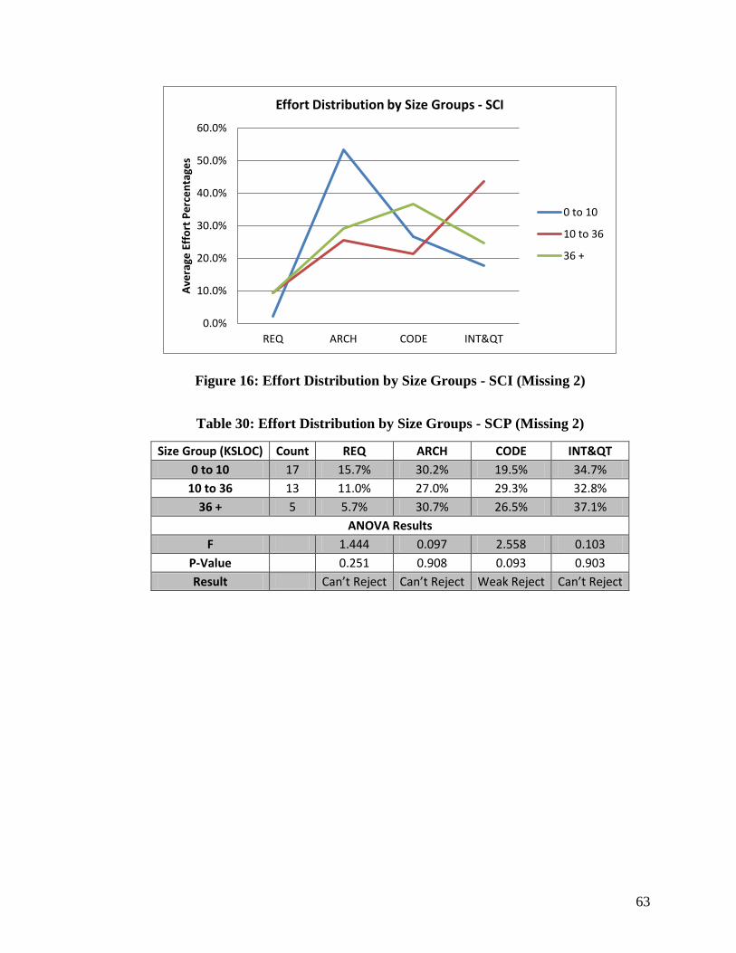
63

Figure 16: Effort Distribution by Size Groups - SCI (Missing 2)

Table 30: Effort Distribution by Size Groups - SCP (Missing 2)


0 to 10 17 15.7% 30.2% 19.5% 34.7%

10 to 36 13 11.0% 27.0% 29.3% 32.8%

36 + 5 5.7% 30.7% 26.5% 37.1%

ANOVA Results

F 1.444 0.097 2.558 0.103

P-Value 0.251 0.908 0.093 0.903

Result Can’t Reject Can’t Reject Weak Reject Can’t Reject

0.0%

10.0%

20.0%

30.0%

40.0%

50.0%

60.0%


Ave

rage

Eff

ort

Pe

rce

nta

ges

Effort Distribution by Size Groups - SCI

0 to 10

10 to 36

36 +

64

Figure 17: Effort Distribution by Size Groups - SCP (Missing 2)

From these results, the only detected trends are 1) Architecture & Design efforts

decrease with size growth as Integration and Qualification Testing efforts increase with

size growth in the Real Time Embedded productivity type; and similarly, 2) Integration &

Qualification Testing efforts increase in the Vehicle Control productivity type with size

growth while both Planning & Requirements and Architecture & Design efforts drop as

size increases. There are no additional interesting points found in the three productivity

types from the “Missing 2” set.

Although the total number of productivity types that can be analyzed is higher

than that of application domains, the overall quality of the analysis results is not much

better. Again, the lack of data points may be the main contributor to inhibiting results.

Increasing the data count seems to be the only strategy for improving this analysis.

0.0%

5.0%

10.0%

15.0%

20.0%

25.0%

30.0%

35.0%

40.0%


Ave

rage

Eff

ort

Pe

rce

nta

ges

Effort Distribution by Size Groups - SCP

0 to 10

10 to 36

36 +

65

4.4 Data Analysis of Personnel Capability


Unlike analysis of project size, analysis of personnel rating does not lack data

points. Data points are not divided into smaller groups and each application domain can

be studied with all of its data points together. Following the guideline described in

Section 3.5.1, each data point is attached with an overall personnel rating. For each

activity group of each application domain, the personnel ratings are plotted against the

effort percentages, and a calculated regression line represents the correlation between

personnel rating and effort distribution. The following table summarizes the results. Note

that Spacecraft Bus is ignored because its personnel ratings are all the same.

Table 31: Personnel Rating Analysis Results - Application Domains

Application Domain

Perfect Set Missing 2 Set Remark

Business Regression lines have notable slope for Architecture & Design and Code & Unit Testing activity groups. R2 is about 30%. Flat for the other activity groups (R2 < 2%).

R2 drops for all activity groups and regression lines become more horizontal.

Not a lot of data points to take in account of analysis. Chances of noise in significant results are high.

Command & Control

Flat regression lines for all activity groups. Low R2 below 10%.

Same as in the Perfect Set.

Data points almost double from the Perfect Set to the Missing 2 Set.

Communication Flat regression lines for all activity groups. Low R2 below 5%.


66

Table 31, Continued

Control and Display

Strong correlation with notable regression lines. High R2 above 80%.

Flatter regression lines and significant drop of R2 (<10%).

Personnel ratings are basically same in the Perfect Set to create strong correlation. Once become different in the Missing 2 Set, regression lines become flatter.

Mission Management

Flat regression lines for all activity groups. Low R2 below 10%.


Mission Planning

Notable regression line for Requirements & Planning. Others are poor (Low R2 below 10%).

Improves regression lines for Code & Unit Testing and Integration & Qualification Testing.

Sensor Control and Processing

Notable regression lines (Fair R2 around 20%) except Code & Unit Testing.

Flatter regression lines result a drop of R2 to below 10%.


Simulation Good regression lines for Architecture & Design and Code & Unit Testing (R2 around 30%).


Weapons Delivery & Control

Strong correlation indicated for Code & Unit Testing and Integration & Qualification Testing (R2 around 50%). Good regression line for Requirements & Planning (R2 around 35%) and fair for Architecture & Design (R2 around 18%).

Much flatter regression lines and significant drop of R2 (below 10%).


As shown in the table above, most application domains produce below-par

regression results that reject the use of personnel ratings as an extra factor in the effort

67

distribution model. The only strong result is from Weapons Delivery & Control, yet the

significant drop of R2 in the Missing 2 Set eliminates it as favorable evidence.

In summary, the results of analyzing Project Size and Personnel Rating provide

more information about application domain’s characteristics and behaviors regarding

effort distribution patterns. However, because of the limitations in either data point

counts or correlation determination values, neither factor can be used with high

confidence to further enhance the domain-based effort distribution model. Thus, neither

will be included in the model architecture if application domains are to be used as the

final domain breakdown.


Mimicking the approach for the application domains analysis, the following table

lays out the results from analyzing productivity types with regard to personnel ratings.

Table 32: Personnel Rating Analysis Results - Productivity Types

Productivity Types

Perfect Set Missing 2 Set Remark

ISM (Infrastructure Middleware)

Strong correlation for Architecture & Design and Code & Unit Testing (R2 above 60%). However, poor for Requirements & Planning and Integration & Qualification Testing (R2 below 3%).

All activity groups produce flatter regression line. R2 drops below 3%.

Data points double from Perfect Set to Missing 2 Set.

MP (Missing Processing)

All activity groups produce flat regression lines.

Same as the Perfect Set.


68

Table 32, Continued

PLN (Planning and Support Activities)

Most activity groups produce good regression lines (R2 above 30%) while Integration & Qualification Testing results poor regression line (R2 below 3%).

Requirements & Planning and Code & Unit Testing stay good (R2 around 25%). Architecture & Design become flatter (R2 drops to below 1%). However, Integration & Qualification Testing improves the regression result (R2 increases to 13%).

RTE (Real-Time Embedded)

All activity groups produce flat regression lines.

Worse results than the Perfect Set.

SCI (Scientific) All activity groups produce flat regression lines.


SCP (Sensor Control and Processing)

All activity groups produce flat regression lines except Code & Unit Testing with a relatively better line (R2 hits 18%).



SYS (System) Good regression results for Architecture & Design and Code & Unit Testing (R2 above 22%). Poor for the others (R2 below 2%).

Worse results than the Perfect Set: Architecture & Design becomes flatter (R2 drops to 16%).

VC (Vehicle Control)

Good regression results for Requirements & Planning and Integration & Qualification Testing (R2 above 30%). Poor for the others (R2 below 2%).

Slightly change in Integration and Qualification Testing (R2 drops to 38%).

69

Similar to Application Domains, there no strong evidence to back the use of

personnel ratings for the effort distribution model. Most productivity types suggest poor

correlation between personnel ratings and effort percentages as indicated by the low R2

values.

Again, productivity types provide no better conclusion than application domains,

and eliminating the project size and personnel rating as additional factors for the effort

distribution model seems reasonable. Overall, by analyzing productivity types, we are

able to produce a list of comparable evidence that we can use to decide which breakdown

is best for the final model. The full detail of this comparison is covered in the next section

and a final decision can be made thereafter.

4.5 Comparison of Application Domains and Productivity Types

In order to build the domain-based effort distribution model, one of the domain

breakdowns must be selected and used as the primary domain definition set, which is to

be supported by the model. In this section, the comparison analysis is described in detail

to show the evaluation of the two analyzed domain breakdown. This analysis will help to

determine the best breakdown based on the following dimensions:

1) Effort distribution patterns and trends.

2) Statistical tests results.

3) Other non-tangible advantages.

Before exploring the detailed comparisons, note that the actual number of

analyzed data points is slightly different between application domains and productivity

70

types. This is mainly because application domains have more domains that reach the

minimum number of records to analyze (10 domains with 5 or more data points) than

productivity types (8 types with 5 or more data points). To sum up this statistic, the total

numbers of data points analyzed for application domains are 122 and 223 for the “Perfect”

set and “Missing 2” set respectively. The total numbers for productivity types are 118 and

219 for the “Perfect” set and “Missing 2” set respectively. Since the “Missing 2” set is a

predicted set that does not fully represent the actual distribution, the comparison analysis

will be conducted solely on the results produced from the “Perfect” set.

Effort Distribution Patterns:

In effort distribution patterns, there are three factors to investigate for application

domains and productivity types:

1) How big are the gaps between the minimum and the maximum average effort

percentages for each activity group? A wider gap indicates larger differences

between domains or types that provide better evidence as strong candidate to

use for the model.

2) How are the trend lines spread between these gaps? Evenly distributed trend

lines indicate that the difference between domains or types is normally

distributed; thus it makes more sense to use this breakdown.

3) How is the general shape of the trend lines different between application

domains and productivity types? If the general shape is the same, there is no

reason to use a separate breakdown.

71

The following two tables summarize the size of the gaps between the minimum

and maximum average effort percentages for all activity groups. Notice that the gap for

Planning & Requirements of productivity types is almost half the size of the gap for

application domains. There is a similar difference for Integration & Qualification Testing,

in that application domains have a much larger gap compared to that of the productivity

types. On the other hand, a wider gap is found for Code & Unit Testing from productivity

types than that of the application domains. However, the magnitude of the gap is not as

wide as we observed in Planning & Requirements or Integration and Qualification

Testing. Therefore, its advantages for productivity types are limited.

Table 33: Effort Distribution Patterns Comparison

Activity Group

Plan & Requirements Architecture & Design

Min Max Diff Min Max Diff

Application Domain 7.78% 33.04% 25.26% 12.45% 45.74% 33.29%

Productivity Type 7.38% 20.56% 13.18% 12.27% 45.20% 32.93%

Table 34: Effort Distribution Patterns Comparison

Activity Group

Code & Unit Testing Integration and QT

Min Max Diff Min Max Diff

Application Domain 22.29% 44.32% 22.03% 16.30% 41.29% 24.99%

Productivity Type 20.34% 50.78% 30.44% 20.67% 34.80% 14.13%

72

Trend lines from both application domains and productivity types are evenly

distributed between the gaps for almost all activity groups. Most application domains are

below 22% for Plan & Requirements, while Spacecraft Bus goes beyond 30%. Most

productivity types squeeze in between 35% and 25% for Code & Unit Testing, while

PLN hits 50%, and MP drops to 20%. In general, the distribution suggests that both

application domains and productivity types are good candidates to produce different


As for the general trend line shapes, these two breakdowns are quite different.

Application domains seem to have wide gaps for all activity groups, whereas productivity

types generates large gap for Architecture & Design and Code and Unit Testing while

closer together for Plan & Requirements and Integration and Qualification Testing.

Statistical Tests Results:

The statistical tests results are straight forward. Tables below outline the

comparison between application domains and productivity types in terms of ANOVA and

T-Test results.

73

Table 35: ANOVA Results Comparison

Activity Group

Application Domain Productivity Type

F P-

Value Results F

P-Value

Results

Plan & Requirements 2.9461 0.0035 Reject 1.9431 0.0694 Reject

Architecture & Design 4.5656 0.0000 Reject 4.9696 0.0000 Reject

Code & Unit Testing 2.1018 0.0350 Reject 3.8851 0.0008 Reject


3.7787 0.0003 Reject 1.9848 0.0634 Reject

Table 36: T-Test Results Comparison

Activity Group COCOMO Averages

Application Domain Productivity

Type

Plan & Requirements

6.5%

All domains reject except Control and Display, Sensor

Control, and Simulation domains.

All types reject except ISM, SCI,

and SCP.


39.3%

All domains reject except Control and Display, Sensor

Control, and Simulation domains.

All types reject except SCI and

SCP.

Code & Unit Testing

30.8% Only Mission Planning

rejects. Only PLN, RTE, and SCP reject.

Integration and Qualification

Testing

23.4%

Only Mission Management, Spacecraft Bus, and

Weapon Delivery domain reject.

Only MP, RTE, and SYS reject.

74

In terms of ANOVA results, application domains are more favorable because of

the low P-values for all activity groups, which give us a 95% confidence level to support

the hypothesis. On the other hand, productivity types perform very well in the T-Test,

giving more rejections to differentiate against the COCOMO II averages – especially in

Code & Unit Testing.

Non-tangible advantages:

There are three subject areas where we study the characteristics and behaviors of

the domain breakdowns:

1) Identifiability: How are domains or types identified? Is the way to identify

domains or types consistent and/or easy?

2) Availability: When can we identify the domain or type in the software

lifecycle?

3) Supportability: How much data can we collect for each breakdown now and in

the future?

Application domains are identified based on the project’s primary functionalities

or capabilities. Since most projects start off with higher level requirements that focus on

functionalities or capabilities, application domain can be easily identified based on the

initial operation description, thus making application domain available before further

requirement analysis and/or design. This early identification also contributes to shrinking

the Cone of Uncertainty effect. Additionally, since the application domains are

categorized by functionalities, the domain definitions are more precise and easier to

75

understand. Many people can relate to the functionalities to draw boundaries between

domains; and therefore, eliminate confusion and overhead between application domains.

On the other hand, in order to identify productivity type, we need both

identification of the application domain and estimation of productivity rate. The

additional estimation may delay the overall identification time since there are no straight

forward references to append productivity rate to a given application domain. Projects

from the same application domain may have a wide range of productivity rates that

depend on additional estimation parameters such as size and personnel information.

Moreover, because a given productivity type may contain several application domains

that summarize a range of functionalities or capabilities, the definition of a productivity

type may not be easily interpreted by project managers who are not familiar with its

concept.

In summary, application domains are more uniform in term of definition clarity

and determination factor. Both revolve around project functionality or capability;

whereas productivity types may jump around between functionality, size, personnel

information, and other necessary parameter to estimate its productivity rate.

Lastly, application domain will have more data support since it is widely used by

many organizations as standard meta-information for software projects and attached to

data collection surveys. In contrast, productivity types are fairly novel such that many

people are not familiar with them, and therefore, project data are not collected with

productivity type information.

76

4.6 Conclusion of Data Analyses

After analyzing the application domains and productivity types, three important

findings emerge:

1) Effort distribution patterns are impacted by project domains.

2) Project size was not confirmed as a source of effort distribution variation.

3) Personnel capability was not confirmed as a source of effort distribution

variation.

With these important findings, I am confident that the domain-based effort

distribution model is a necessary alternative to enhance the overall effort distribution

guidance that is currently available in the COCOMO II model.

Having compared the application domains and productivity types, I’ve concluded

that application domains are more relevant and usable as the key domain definition set (or

breakdown structure) to be supported by the domain-based effort distribution model as it

is more uniform to use and has better data support over the productivity types.

77

CHAPTER 5: DOMAIN-BASED EFFORT DISTRIBUTION MODEL

This chapter presents detailed information about the domain-based effort

distribution model. Section 5.1 provides a comprehensive description of the model

including its inputs and outputs, general structure, and key components. Section 5.2

outlines an implementation instance of the model and its connection to a copy of the

COCOMO II model implementation. This section also provides a simple guide to using

the implemented tool to estimate effort distribution of a sample project.

5.1 Model Description

As depicted in the following figure, the domain-based effort distribution model

takes project effort (in person-month) and application domain as the primary inputs and

produces a suggested effort distribution guideline as its main output. It is designed as an

extension model for the COCOMO II model and follows a similar reporting fashion to

display the output effort distribution. Effort distribution is reported in a tabular format in

terms of development phase (or activity group), phase effort percentages, and phase effort

in person-months.

78

Figure 18: Domain-based Effort Distribution Model Structure

The suggested effort distribution is a product of total project effort and average

effort percentages. Average effort percentages are determined using a look up table of

application domains and activity groups. This table is shown below. If no application

domain is provided with the project, the suggested effort distribution will fall back to the

standard COCOMO II waterfall effort distribution.

79

Table 37: Average Effort Percentages Table for the Domain-Based Model

Average Effort Percentages

Application Domains Requirement Arch &

Design

Code & Unit

Test

Integration &

QT

Business 20.98% 22.55% 24.96% 31.51% Command & Control 21.04% 22.56% 33.73% 22.66% Communications 14.95% 30.88% 28.54% 25.62% Control & Display 14.72% 34.80% 24.39% 26.09% Mission Management 15.40% 17.78% 28.63% 38.20% Mission Planning 17.63% 12.45% 44.32% 25.60% Sensors Control and

Processing 7.78% 45.74% 22.29% 24.19%

Simulation 10.71% 39.11% 30.80% 19.38% Spacecraft Bus 33.04% 20.66% 30.00% 16.30% Weapons Delivery and

Control 11.50% 17.39% 29.82% 41.29%

These above listed application domains have a sufficient number of data points in

the “Perfect” set, and their average effort percentages are also calculated from the

“Perfect” set. Additionally, we can add those with enough data points in the “Missing 2”

set, namely Infrastructure and Middleware and Tool and Tool Systems. We can note

these application domains as predicted domains, and we need to be aware of their

limitation of data support when using the suggested effort distribution.

5.2 Model Implementation

In order to demonstrate how the model works, I developed an implementation

instance of the model. This instance is built on top of a web-based COCOMO II tool that

80

was developed earlier for demonstration. This tool runs on Apache web server, using

MySQL database, and written in PHP and JavaScript.

The mathematical formulation used for this implementation is as follows:

From the COCOMO II model, the total project effort (PM) is computed as

∏

(EQ. 5)

where ∑ (EQ. 6)

EM is the COCOMO II effort multiplier and SF is scale factor.

For each supported application domain ADk, effort can be computed as

( ) ( ) (EQ. 7)

( ) ( ) (EQ. 8)

( ) ( ) (EQ. 9)

( ) ( ) (EQ. 10)

The percentage for each equation comes from Table 37.

Figure 19 captures the main screen of a sample project. The general information

of the project is displayed in the top portion including project name, application domain,

operating environment, development method, scale factors, and schedule constraints.

Modules can be added to the project using the add module button. Each module will need

input of language, labor rate, size, and EAF. Size can be calculated in three modes:

adapted code, function point conversion, and simple SLOCs. EAF is calculated by setting

values for 16 effort multipliers from the COCOMO II model. The estimation results are

displayed at the bottom. Effort, schedule, productivity, costs, and staff are calculated

based on the project input. Three levels of estimates are produced: optimistic, most likely,

81

and pessimistic. An effort distribution link is available next to the Estimation Results

label. Clicking on it will bring the effort distribution screen to the user.

Figure 19: Project Screen of the Domain-based Effort Distribution Tool

The following figure shows the suggested domain-based effort distribution of a

Weapon Delivery and Control project. The total project effort is 24.2 PM, and the

suggested percentages and actual PM for each activity group is listed at the bottom

portion of the display area. A column graph is also produced to illustrate the effort

distribution visually. Both COCOMO II Waterfall and MBASE effort distribution are

also available for the user to compare results.

82

Figure 20: Effort Results from the Domain-base Effort Distribution Tool

5.3 Comparison of Domain-Based Effort Distribution and COCOMO

II Effort Distribution

This section will validate and compare the results produced using the domain-

based effort distribution against the results from the COCOMO II model.

Data Source:

83

Three sets of sample projects are used for this comparison. The sample projects

come from the original COCOMO II calibration data which contains sufficient

information including domain information, project size, COCOMO II drivers’ values, and

schedule constraints. The sample projects are also attached with most of the actual effort

distribution data in PM for each activity group or waterfall phase.

The details of these sample projects are described in the following table. Note that

there are no requirements or planning effort data for project 51 and 62. In fact, the only

data points that I can find with requirements & planning effort data is from project 49.

The requirements and planning effort data was not required in the earlier data collection

survey, therefore, most projects submitted the survey without that effort data.

Table 38: Sample Project Summary

ID Application Domain Size (KSLOC) Effort (PM) Phase Effort (PM)

REQ ARCH CUT INT&QT

49 Command and Control 142.8 631 90 136 273 132

51 Communication 127.05 499 NA 145 199 155

62 Simulation 171 812.1 NA 303.7 406.7 101.7

Comparison Steps:

The procedure for the comparison analysis is straight forward. For each sample

project, the following steps are performed to collect a final result that I can use to

evaluate the performance of the domain-based effort distribution model:

1) Create a project with necessary information (domain information, size, name,

etc.) using the tool; add COCOMO II drivers’ value accordingly.

84

2) Collect the output effort distribution for both COCOMO II Waterfall and

Domain-based effort distribution model.

3) Compare the effort distributions with the actual effort distribution of the

project.

4) Calculate the errors of each estimated effort distribution and determine which

produces the best results.

Analysis Results:

Using the tool, the following estimated total efforts are produced from the

COCOMO II model for the sample projects:

Table 39: COCOMO II Estimation Results

ID Actual Effort (PM) Estimated Effort (PM) Estimation Error

49 631 1094.3 +73.4%

51 499 856.7 +71.7%

62 812.1 586.6 -27.8%

Next, I produced a series of comparison tables that compares the COCOMO II

Waterfall effort distribution results against results produced using the domain-based

effort distribution model.

85

Project 49 (Command and Control):

Table 40: Project 49 Effort Distribution Estimate Comparison

COCOMO II Domain-based Effort Distribution

Activity Group Est. PM Error Est. PM Error

Requirements 87.54 -2.70% 229.8 153.30%

Architecture 196.97 44.80% 247.31 81.80%

Code & Unit Test 556.78 103.90% 368.78 35.10%

Integration & QT 340.55 158.00% 248.41 88.20%

Total Error 194.00% 199.00%

Project 51 (Communications):




Requirements 68.54 NA 128.51 NA

Architecture 154.21 6.40% 290.42 100.30%

Code & Unit Test 437.17 119.70% 244.16 22.70%

Integration & QT 265.32 71.20% 219.32 41.50%

Total Error 139.39% 110.88%

Project 62 (Simulations):




Requirements 35.2 NA 62.77 NA

Architecture 93.86 -69.10% 229.36 -24.50%

Code & Unit Test 346.09 -14.90% 180.67 -55.60%

Integration & QT 146.65 44.20% 113.8 11.90%

Total Error 83.38% 61.88%

86

In each result table, the estimated efforts are produced for each Waterfall phase or

activity group by its respective effort distribution model. Error for each activity group is

calculated against the actual efforts. The total error is the sum of the individual error and

can be used as the final evaluation value for this comparison.

The results suggest that COCOMO II Waterfall produces slightly better results in

project 49 (194% total error vs. 199% total error), but somewhat worse results in project

51 and project 62 (generally +20% worse than the domain-based effort distribution

results). In the COCOMO II Waterfall’s defense, missing the requirements and planning

phase results may cause a drop in performance in project 51 and project 62. The counter

argument is that the COCOMO II effort distribution does not take account of the

requirements and planning effort in general, as it was not part of the COCOMO II model

calibration (also a reason the effort data was not required in the data collection survey).

This may also undermine the better results from project 49. The good results for

estimated requirements and planning effort may have been produced merely by chance. If

only considering the other three activity groups, the results are 194% vs. 125%. The

domain-based effort distribution model produces a much better estimate. Another

important point is that these sample projects are selected from the calibration data points

for the COCOMO II model, and therefore should fit the COCOMO II Waterfall better

since the domain-based effort distribution model is based on an entirely different data set.

To sum up, the domain-based effort distribution model produces a better estimate

if we ignore requirements and planning effort (less error if we only sum up errors from

Architecture & Design, Code & Unit Testing, and Integration & Qualification Testing).

87

Although the evaluation result suggests that the domain-based effort distribution model

performs fairly well against the COCOMO II Waterfall, at least for three of the four

activity groups, there is definitely need for further validation tests to confirm the

advantage.

88

CHAPTER 6: RESEARCH SUMMARY AND FUTURE WORKS

6.1 Research Summary

The central theme of this research revolves around finding the relationship

between software project information and effort distribution patterns, particular project

domain, size, and personnel rating. Such a relationship was discovered for domain

information, but was not for size and personnel rating. Since the domain is usually easy

to define in the early stage of a project lifecycle, it can provide substantial improvement

in preparing resource allocation plans for the different stages of software development.

For data and domains analyzed, the hypothesis test strongly confirms such a relationship.

And as a result, a new domain-based effort distribution model is drafted and we are one

step further in improving the already-popular COCOMO II model for the data-supported

application domains.

In this research, two sets of domain breakdowns, namely application domains and

productivity types, are analyzed for their correlations to effort distribution patterns. A

data support of 530 project records is used for this analysis. Both visual and statistical

tests are conducted to prove the significance of domain as an influential driver on effort

distribution patterns. Project size and personnel rating are studied to determine additional

factors that may cause distinguishable trends within domain or type. Comparison between

application domains and productivity types helps to determine the domain breakdown

89

that can be used for the domain-base effort distribution model, which is designed and

implemented as a prototype to attach to the COCOMO II model as a new extension

model. Finally, estimation results produced from several sample projects are compared

against those produced from the original COCOMO II Waterfall effort distribution

guideline to test the performance of the domain-based effort distribution model. Although

the results of this comparison do not favor any model in a huge fashion, it is encouraging

to see desirable numbers produced from the domain-based effort distribution model.

6.2 Future Work

After this research, the main goal is to continue refining the domain-based effort

distribution model. There are several known improvements that are beneficial to

complete:

1) Refine the overall effort distribution patterns of the existing supported

application domains when more data points become available.

2) Support more application domains when more data points become available.

3) Test hypotheses about whether similar results will emerge in sections other

than the defense industry.

Other than improvement works on existing model features, the following studies

can be completed to add valuable extension features to the model:

1) Expand the model to include the schedule distribution patterns available in the

current COCOMO II model for Waterfall and MBASE distribution guideline.

90

2) Study the effects of operating environments, which state the physical

constraint of software systems; and explore the possibility of adding operating

environment as a new dimension to influence both effort distribution patterns

and schedule distribution patterns.

3) Study the relationships between COCOMO II drivers and domain information;

seek possible correlations that can help to enhance the domain-based effort

distribution model.

91

REFERENCES

[AFCAA, 2011] Air Force Cost Analysis Agency (AFCAA). Software Cost Estimation

Metrics Manual. 2011.

[Aroonvatanaporn, 2012] Aroonvatanaporn, P. “Shrinking the Cone of Uncertainty with

Continuous Assessment for Software Team Dynamics in Design and Development”. USC CSSE,

PhD Dissertation. 2012.

[Au Yeung] Au Yeung, C. “Matrix Factorization: A Simple Tutorial and Implementation in

Python”. http://www.albertauyeung.com/mf.php.

[Blom, 1958] Blom, G. Statistical estimates and transformed beta variables. John Wiley and Sons.

New York. 1958.

[Boehm, 2010] Boehm, B. “Future Challenges and Rewards of Software Engineers”. Journals of

Software Technology, Vol. 10, No. 3, October 2010.

[Boehm, 2000] Boehm, B., et al. Software Cost Estimation with COCOMO II. Prentice Hall, NY.

2000.

[Boehm, 1981] Boehm, B. Software Engineering Economics. Prentice Hall, New Jersey. 1981.

[Borysowich, 2005] Borysowich, C. “Observations from a Tech Architect: Enterprise

Implementation Issues & Solutions – Effort Distribution Across the Software Lifecycle”.

Enterprise Architecture and EAI Blog. http://it.toolbox.com/blogs/enterprise-solutions/effort-

distribution-across-the-software-lifecycle-6304. October 2005.

[DCRC, 2005] Defense Cost and Resource Center. “The DoD Software Resource Data Report –

An Update.” Practical Software Measurement (PSM) Users’ Group Conference Proceedings. July

2005.

[DoD HDBK, 2005] Department of Defense Handbook. “Work Breakdown Structure for Defense

Material Items: MIL-HDBK-881A.” July 30, 2005.

[Digital, 1991] Digital Equipment. VAX PWS Software Source Book. Digital Equipment Corp.,

Maynard, Mass., 1991.

[Galorath, 2005] Galorath Inc. SEER-SEM User Manual. 2005.

[Heijistek, 2008] Heijstek, W., Chaudron, M.R.V. “Evaluating RUP Software Development

Process Through Visualization of Effort Distribution”. EUROMICRO Conference Software

Engineering and Advanced Application Proceedings. 2008. Page 266.

http://www.albertauyeung.com/mf.php

http://it.toolbox.com/blogs/enterprise-solutions/effort-distribution-across-the-software-lifecycle-6304.%20October%202005



92

[IBM, 1988] IBM Corporation. Industry Applications and Abstracts. IBM. White Plains, N.Y.,

1988.

[Jensen, 1983] Jensen, R. “An Improved Macrolevel Software Development Resource

Estimation Model”. Proceedings 5th

ISPA Conference. April 1983. Page 88.

[Kruchten, 2003] Kruchten, P. The Rational Unified Process: An Introduction. Addison-Wesley

Longman Publishing Co., Inc. Boston. 2003.

[Kultur, 2009] Kultur, Y., Kocaguneli, E., Bener, A.B. “Domain Specific Phase By Phase Effort

Estimation in Software Projects”. International Symposium on Computer and Information

Sciences. September 2009. Page 498.

[Lee, 2001] Lee, D., Seung, H.S. “Algorithms for Non-negative Matrix Factorization.” Advances

in Neural Information Processing Systems 13: Proceedings of the 2000 Conference. MIT Press.

pp. 556–562. 2001.

[McConnell, 2006] McConnell, S. Software Estimation Demystifying the Black Art, Microsoft

Press, 2006, page 62.

[Norden, 1958] Norden, P.V. “Curve Fitting for a Model of Applied Research and Development

Scheduling”. IBM J. Research and Development. 1958. Vol. 3, No. 2, Page 232-248.

[NAICS, 2007] North American Industry Classification System,

http://www.census.gov/eos/www/naics/, 2007.

[O’Connor, 2003] O'Connor, J. Robertson, E. "Student's t-test", MacTutor History of

Mathematics archive, University of St Andrews, http://www-history.mcs.st-

andrews.ac.uk/Biographies/Gosset.html, 2003.

[Pearson, 1901] Pearson, K. "On the criterion that a given system of deviations from the probable

in the case of a correlated system of variables is such that it can be reasonably supposed to have

arisen from random sampling". Philosophical Magazine, Series 5 50 (302), 1901. Page 157–175.

[Port, 2005] Port, D. Chen, Z. Kruchten, P. “An Empirical Validation of the RUP ‘Hump’

Diagram”. Proceedings of the 4th

International Symposium on Empirical Software

Engineering. 2005.

[PRICE, 2005] PRICE Systems. True S User Manual. 2005.

[Putnam, 1976] Putnam, L.H. “A Macro-Estimating Methodology for Software Development”.

IEEE COMPCON 76 Proceedings. September 1976. Page 138-143.

[Putnam, 1992] Putnam, L. and Myers. W. Measures for Excellence. Yourdon Press Computing

Series. 1992.

[QSM] Quantitative Software Management (QSM) Inc. SLIM-Estimate www.qsm.com.

http://www-history.mcs.st-andrews.ac.uk/Biographies/Gosset.html



http://www.qsm.com/

93

[Reifer, 1990] Reifer Consultants. Software Productivity and Quality Survey Report. El Segundo,

Calif., 1990.

[Shapiro, 1965] Shapiro, S. S.; Wilk, M. B. “An analysis of variance test for normality (complete

samples).” Biometrika 52 (3-4), 1965: page 591–611.

[Standish, 2009] Standish Group. Chaos summary 2009, 2009. http://standishgroup.com.

[Stephens, 1974] Stephens, M. A. "EDF Statistics for Goodness of Fit and Some Comparisons".

Journal of the American Statistical Association. Vol. 69, No. 347 (Sep., 1974). Page 730-737.

[Upton, 1996] Upton, G., Cook, I. Understanding Statistics. Oxford University Press. Page 55.

1996.

[Yang, 2008] Yang, Y., et al. “Phase Distribution of Software Development Effort”. Empirical

Software Engineering and Measurement. October 2008. Page 61.

94

APPENDIX A: DOMAIN BREAKDOWN

Application Domains:

Name Definition

Business Systems Software that automates business functions, stores and retrieves data,

processes orders, manages/tracks the flow of materials, combines

data from different sources, or uses logic and rules to process

information.

Example:

Management information systems (Personnel)

Financial information systems

Enterprise Resource Planning systems

Logistics systems (Order Entry, Inventory)

Enterprise data warehouse

Other IT systems

Internet Software developed for applications that run and utilize the Internet.

Typically uses web services or middleware platforms (Java, Flash) to

provide a variety of functions, e.g. search, order/purchase and multi-

media.

Example:

Web services

Search systems like Google

Web sites (active or passive) that provide information in multi-

media form (voice, video, text, etc.)

Tool and Tool Systems Software packages and/or integrated tool environments that are used

to support analysis, design, construction and test of other software

applications

Example:

Integrated collection of tools for most development phases of the

life cycle

Rational development environment

Scientific Systems Software that involves significant computational and scientific

analysis. It uses algorithmic, numerical or statistical analysis to

process data to produce information.

Example:

Seismic survey analysis

Experiments run on supercomputers to unravel DNA

95

Name Definition

Simulation and Modeling Software used to evaluate scenarios and assess empirical

relationships that exist between models of physical processes,

complex systems or other phenomena. The software typically

involves running models using a simulated clock in order to mimic

real world events.

Example:

Computer-in-the-loop

Guidance simulations

Environment simulations

Orbital simulations

Signal generators

Test and Evaluation Software used to support test and evaluation functions. This software

automates the execution of test procedures and records results.

Example:

Test suite execution software

Test results recording

Training Software used to support the education and training of system users.

This software could be hosted on the operational or a dedicated

training system.

Example:

On-line courses

Computer based training

Computer aided instruction

Courseware

Tutorials

Command and Control Software that enables decision makers to manage dynamic situations

and respond in real time. Software provides timely and accurate

information for use in planning, directing, coordinating and

controlling resources during operations. Software is highly

interactive with a high degree of multi-tasking.

Example:

Satellite Ground Station

Tactical Command Center

Battlefield Command Centers

Telephone network control systems

Disaster response systems

Utility power control systems

Air Traffic Control systems

Mission Management Software that enables and assists the operator in performing mission

management activities including scheduling activities based on

vehicle, operational and environmental priorities.

Example:

Operational Flight Program

Mission Computer

Flight Control Software

96

Name Definition

Weapons Delivery and Control Software used to select, target, and guide weapons. Software is

typically complex because it involves sophisticated algorithms, fail-

safe functions and must operate in real-time.

Example:

Target location

Payload control

Guidance control

Ballistic computations

Communications Software that controls the transmission and receipt of voice, data,

digital and video information. The software operates in real-time or

in pseudo real-time in noisy environments.

Example:

Radios

Microwave controller

Large telephone switching systems

Network management

Controls and Displays Software that provides the interface between the user and system.

This software is highly interactive with the user, e.g. screens, voice,

keyboard, pointing devices, biometric devices.

Example:

Heads Up Displays

Tactical 3D displays

Infrastructure or Middleware Software that provides a set of service interfaces for a software

application to use for control, communication, event handling,

interrupt handling, scheduling, security, and data storage and

retrieval. This software typically interfaces to the hardware and other

software applications that provide services.

Example:

Systems that provide essential services across a bus

Delivery systems for service-oriented architectures, etc.

Middleware systems

Tailored operating systems and their environments

Executive Software used to control the hardware and operating environment

and to serve as a platform to execute other applications. Executive

software is typically developed to control specialized platforms

where there are hard run-time requirements.

Example:

Real-time operating systems

Closed-loop control systems

Information Assurance Software that protects other software applications from threats such

as unauthorized access, viruses, worms, denial of service, and

corruption of data.

Includes sneak circuit analysis software. A sneak circuit is an

unexpected path or logic flow within a system that, under certain

conditions, can initiate an undesired function or inhibit a desired

function.

Example:

Intrusion prevention devices

97

Name Definition

Maintenance and Diagnostics Software used to perform maintenance functions including detection

and diagnosis of problems. Used to pinpoint problems, isolate faults

and report problems. It may use rules or patterns to pinpoint solutions

to problems.

Example:

Built-in-test

Auto repair and diagnostic systems

Mission

Planning

Software used for scenario generation, feasibility analysis, route

planning, and image/map manipulation. This software considers the

many alternatives that go into making a plan and captures the many

options that lead to mission success.

Example:

Route planning software

Tasking order software

Process Control Software that provides closed-loop feedback controls for systems that

run in real-time. This software uses sophisticated algorithms and

control logic.

Example:

Power plant control

Oil refinery control

Petro-chemical control

Closed loop control-systems

Sensor Control and Processing Software used to control and manage sensor transmitting and

receiving devices. This software enhances, transforms, filters,

converts or compresses sensor data typically in real-time. This

software uses a variety of algorithms to filter noise, process data

concurrently in real-time and discriminate between targets.

Example:

Image processing software

Radar systems

Sonar systems

Electronic Warfare systems

Spacecraft Bus Spacecraft vehicle control software used to control and manage a

spacecraft body. This software provides guidance, attitude and

articulation control of the vehicle.

Example:

Earth orbiting satellites

Deep space exploratory vehicles

Spacecraft Payload Spacecraft payload management software used to manage and

control payload functions such as experiments, sensors or

deployment of onboard devices.

Example:

Sensors on earth orbiting satellites

Equipment on deep space exploratory vehicles

98

Productivity Types:

Name Definitions

Sensor Control and

Signal Processing

(SCP)

Software that requires timing-dependent device coding to enhance, transform,

filter, convert, or compress data signals.

Ex.: Bean steering controller, sensor receiver/transmitter control, sensor

signal processing, sensor receiver/transmitter test.

Ex. of sensors: antennas, lasers, radar, sonar, acoustic, electromagnetic.

Vehicle Control (VC) Hardware & software necessary for the control of vehicle primary and

secondary mechanical devices and surfaces.

Ex: Digital Flight Control, Operational Flight Programs, Fly-By-Wire Flight

Control System, Flight Software, Executive.

Real Time Embedded

(RTE)

Real-time data processing unit responsible for directing and processing sensor

input/output.

Ex: Devices such as Radio, Navigation, Guidance, Identification,

Communication, Controls And Displays, Data Links, Safety, Target Data

Extractor, Digital Measurement Receiver, Sensor Analysis, Flight

Termination, Surveillance, Electronic Countermeasures, Terrain Awareness

And Warning, Telemetry, Remote Control.

Vehicle Payload (VP) Hardware & software which controls and monitors vehicle payloads and

provides communications to other vehicle subsystems and payloads.

Ex: Weapons delivery and control, Fire Control, Airborne Electronic Attack

subsystem controller, Stores and Self-Defense program, Mine Warfare

Mission Package.

Mission Processing

(MP)

Vehicle onboard master data processing unit(s) responsible for coordinating

and directing the major mission systems.

Ex.: Mission Computer Processing, Avionics, Data Formatting, Air Vehicle

Software, Launcher Software, Tactical Data Systems, Data Control And

Distribution, Mission Processing, Emergency Systems, Launch and Recovery

System, Environmental Control System, Anchoring, Mooring and Towing.

Command & Control

(C&C)

Complex of hardware and software components that allow humans to manage

a dynamic situation and respond to user-input in real time.

Ex: Battle Management, Mission Control.

System Software (SYS) Layers of software that sit between the computing platform and applications

Ex: Health Management, Link 16, Information Assurance, Framework,

Operating System Augmentation, Middleware, Operating Systems.

Telecommunications

(TEL)

Transmission and receipt of voice, digital, and video data on different

mediums & across complex networks.

Ex: Network Operations, Communication Transport.

Process Control (PC) Software that controls an automated system, generally sensor driven.

Ex:

99

Scientific Systems

(SCI)

Non real time software that involves significant computations and scientific

analysis.

Ex: Environment Simulations, Offline Data Analysis, Vehicle Control

Simulators

Training (TRN) Hardware and software that are used for educational and training purposes

Ex: Onboard or Deliverable Training Equipment & Software, Computer-

Based Training.

Test Software (TST) Hardware & Software necessary to operate and maintain systems and

subsystems which are not consumed during the testing phase and are not

allocated to a specific phase of testing.

Ex: Onboard or Deliverable Test Equipment & Software.

Software Tools (TUL) Software that is used for analysis, design, construction, or testing of computer

programs

Ex: Integrated collection of tools for most development phases of the life

cycle, e.g. Rational development environment

Business Systems (BIS) Software that automates a common business function

Ex: Database, Data Distribution, Information Processing, Internet,

Entertainment, Enterprise Services, Enterprise Information

Operating Environments:

Name Definition

Fixed Ground Manned and unmanned fixed, stationary land sites (buildings) with access to

external power sources, backup power sources, physical access to systems,

regular upgrades and maintenance to hardware and software, support for

multiple users.

Example:

Computing facilities

Command and Control centers

Tactical Information centers

Communication centers

Mobile Ground Mobile platform that moves across the ground. Limited power sources.

Computing resources limited by platform’s weight and volume constraints.

Upgrades to hardware and software occur during maintenance periods.

Computing system components are physically accessible.

Example:

Tanks

Artillery systems

Mobile command vehicles

Reconnaissance vehicles

Robots

100

Name Definition

Shipboard Mobile platform that moves across or under water.

Example:

Aircraft carriers

Cruisers

Destroyers

Supply ships

Submarines

Avionics Manned airborne platforms. Software that is complex and runs in real-time in

embedded computer systems. It must often operate under interrupt control to

process timelines in the nanoseconds.

Example:

Fixed-wing aircraft

Helicopters

Unmanned Airborne Unmanned airborne platforms. Man-in-the-loop control.

Example:

Remotely piloted air vehicles

Missile Very high-speed airborne platform with tight weight and volume restrictions.

Example:

Air-to-air missiles

Strategic missiles

Manned Space Space vehicle used to carry or transport passengers. Severe power, weight and

volume restrictions.

Example:

Space shuttle

Space passenger vehicle

Manned space stations

Unmanned Space Space vehicle used to carry payloads into space. Severe power, weight and

volume restrictions. Software in this environment is complex and real-time.

Software is subject to severe resource constraints because its platform may

have memory and speed limitations due to weight restrictions and radiation.

Example:

Orbiting satellites (weather, communications)

Exploratory space vehicles

101

APPENDIX B: MATRIX FACTORIZATION SOURCE CODE

Matlab™ Program Source Code:

Main routine:

102

Matrix_fact function:

103

APPENDIX C: COCOMO II DOMAIN-BASED EXTENSION TOOL

AND EXAMPLES

Program Screen Shots:

Opening Screen:

104

Start a project:

Project Scale Drivers:

105

Module Detail:

Module Size:

Module EAF:

106

Project Estimate:

Effort Distribution:

107

Sample Projects Results for COCOMO II Waterfall and Domain-based Effort

Distribution Model Comparison:

Project 49:

108

Project 51:

109

Project 62:

110

APPENDIX D: DCARC SAMPLE DATA REPORT

SRDR form DD 2630-3

domain-based effort distribution model for...

Documents