Does Gender Inequality ReduceGrowth and Development?Evidence from Cross-CountryRegressions

Stephan Klasen

November 1999The World BankDevelopment Research Group/Poverty Reduction and Economic Management Network

POLICY RESEARCH REPORT ONGENDER AND DEVELOPMENTWorking Paper Series, No. 7

The PRR on Gender and Development Working Paper Series disseminates the findings of work in progress to encourage theexchange of ideas about the Policy Research Report. The papers carry the names of the authors and should be cited accordingly.The findings, interpretations, and conclusions are the author’s own and do not necessarily represent the view of the World Bank, itsBoard of Directors, or any of its member countries.Copies are available online at http: //www.worldbank.org/gender/prr.

Gender inequality in educationhas a significant negative impacton economic growth and appearsto be an important factorcontributing to Africa's and SouthAsia's poor growth performanceover the past 30 years. Inaddition to increasing growth,greater gender equality ineducation promotes otherimportant development goals,including lower fertility andlower child mortality.

Does Gender Inequality Reduce Growth and Development?Evidence from Cross-Country Regressions

Stephan KlasenDepartment of Economics

University of MunichGermany

Abstract:Using cross-country and panel regressions, this paper investigates to whatextent gender inequality in education and employment may reduce growth anddevelopment. The paper finds a considerable impact of gender inequality oneconomic growth which is robust to changes in specifications and controls forpotential endogeneities. The results suggest that gender inequality in educationhas a direct impact on economic growth through lowering the average qualityof human capital. In addition, economic growth is indirectly affected throughthe impact of gender inequality on investment and population growth. Pointestimates suggest that between 0.4-0.9 % of the differences in growth ratesbetween East Asia and Sub Saharan Africa, South Asia, and the Middle Eastcan be accounted for by the larger gender gaps in education prevailing in thelatter regions. Moreover, the analysis shows that gender inequality ineducation prevents progress in reducing fertility and child mortality rates,thereby compromising progress in well-being in developing countries.

I would like to thank Jere Behrman, Chitra Bhanu, Mark Blackden, Lionel Demery, David Dollar, BillEasterly, Diane Elson, Roberta Gatti, Beth King, Andy Mason, Claudio Montenegro, Susan Razzaz, LynSquire, Martin Weale, Jeffrey Williamson, and participants at a research seminar in Munich and aworkshop in Oslo for helpful comments and discussion on earlier versions of this paper. I also want tothank Frank Hauser for excellent research assistance.

1

I. Introduction

Many developing countries exhibit considerable gender inequality in education,

employment, and health outcomes. For example, girls and women in South Asia and China suffer

from elevated mortality rates which have been referred to as the ‘missing women’ by Amartya Sen

and others (Sen, 1989; Klasen, 1994). In addition, there are large discrepancies in education

between the sexes in South Asia and Sub Saharan Africa. Finally, employment opportunities and

pay differ greatly by gender in most developing regions (and some developed ones as well, see

UNDP, 1995).

When assessing the importance of these gender inequalities, one has to distinguish between

intrinsic and instrumental concerns. If our concern is with aggregate well-being as measured by,

for example, Sen’s notion of ‘capabilities’ (Sen, 1999), then we should view the important

capabilities of longevity and education as critical constituent elements in well-being. Thus any

reduced achievements for women in these capabilities is intrinsically problematic.1

In addition, one may be concerned about gender equity as a development goal in its own

right (apart from its beneficial impact on other development goals) as has been, for example,

recognized in the Convention on the Elimination of All Forms of Discrimination against Women

(CEDAW) which has been signed and ratified by a majority of developing countries. If this is our

concern, there is no need to go further than demonstrating inequity in a particular country, which

would, in and of itself, justify corrective action.

Apart from these intrinsic problems of gender inequality, one may be concerned about

instrumental effects of gender bias. Gender inequality may have adverse impacts on a number of

valuable development goals. First, gender inequality in education and access to resources may

prevent a reduction of child mortality, of fertility, and an expansion of education of the next

generation. To the extent that these linkages exist, gender bias in education may thus generate

instrumental problems for development policy-makers as it compromises progress in other

important development goals.

Secondly, it may be the case that gender inequality reduces economic growth. This is an

important issue to the extent that economic growth furthers the improvement in well-being (or at

least enables the improvement in well-being). That economic growth, on average, furthers well-

being (measured through indicators such as longevity, literacy, and reduced poverty) has been

demonstrated many times, although not all types of growth do so to the same extent (Drèze and

Sen, 1989; UNDP, 1996; Bruno, Squire, and Ravallion, 1996; Pritchett and Summers, 1996).

2

Thus policies that further economic growth (and do not harm other important development goals)

should be of great interest to policy-makers all over the world.

This paper is concerned with the instrumental impact of gender inequality in education

(and, to a lesser extent, employment). Using cross-country regressions, it tries to determine to what

extent gender bias has a negative impact on economic growth, and to what extent it prevents

reductions in fertility and child mortality. The paper shows that gender bias in education and

employment appears to have a significant negative impact on economic growth. It also leads to

higher fertility and child mortality. The effects account for a considerable portion of the

differences in growth experience between the developing regions of the world. In particular, South

Asia and Sub-Saharan Africa are held back by high gender inequality in education and

employment.

The paper is organized as follows. Section 2 reviews insights from the theoretical and

empirical growth literature as they pertain to the possible effect of gender inequality. Section 3

discusses several possible reasons why gender inequality in education and employment may retard

growth and development. Section 4 describes the data and the econometric specifications. Section

5 presents descriptive statistics, and Section 6 contains the main empirical results. Section 7

concludes.

II. Gender and Economic Growth: Theoretical and Empirical Linkages

Recent years have seen a renewed interests in the theoretical and empirical determinants of

economic growth. On the theoretical front, Roemer (1986), Lucas (1988), and Barro and Sala-i-

Martin (1995) have emphasized the possibility of endogenous growth where economic growth is

not constrained by diminishing returns to capital. These models stand in contrast to Solow (1956)

which, based on a neo-classical production function (with diminishing returns to each input) and

exogenous savings and population growth, suggested convergence of per capita incomes,

conditional on exogenous savings and population growth rates. Many of these models have also

emphasized the importance of human capital accumulation for economic growth. The inclusion of

human capital can be achieved within the traditional Solow model and still yield conditional

convergence; or it can also be incorporated into (and indeed be a major reason behind) endogenous

growth models (Mankiw, Roemer, and Weil, 1992).2

There are few models that explicitly consider gender inequality in education and its impact

on economic growth. One paper by Lagerlöf (1999) examines the impact of gender inequality in

education on fertility and economic growth. Using an overlapping generations framework, the

3

paper argues that initial gender inequality in education can lead to a self-perpetuating equilibrium

of continued gender inequality in education, with the consequences of high fertility and low

economic growth.3 In this model, gender inequality in education may generate a poverty trap which

would justify public action to escape this low-level equilibrium with self-perpetuating gender gaps

in education.

On the empirical front, the development of new international panel data sets has, for the

first time, allowed sophisticated time series, cross-section, and panel analysis of the determinants of

long-run growth (Barro, 1991; Mankiw, Roemer, and Weil, 1992, Barro and Sala-i-Martin, 1995;

ADB, 1997). These empirical models combine insights from the theoretical literature (esp. the

issue of convergence and the importance of savings, population growth rates, and human capital

accumulation) with largely ad hoc specifications that may be seen to proxy for differences in the

technological shift parameter (broadly conceived) of the production function between different

countries. These shift parameters thus effect the steady-state level of GDP (in conditional

convergence models) or the long-term growth rates (in endogenous growth models). Factors

examined in this context include the level of corruption, political instability, ethno-lingual

fractionalization, being landlocked, openness to trade, the quality of public services and

institutions, and the dependency burden (e.g. Barro, 1991; ADB, 1997; Easterly and Levine, 1997;

Collier and Gunning, 1998; Sachs and Warner, 1995; Bloom and Williamson, 1998).

These empirical analyses not only differ in the inclusion of various parameters thought to

influence the steady state level of GDP, but also in the approach to treating the proximate

determinants of economic growth, most notably the investment rate. Some studies have included

the investment rate as one of the explanatory variables (e.g. Mankiw, Roemer, and Weil, 1992;

Barro and Sala-i-Martin, 1995); others have left it out in the belief that the investment rate itself is

determined by some of the other regressors included in the equations, for example the level of

human capital or the quality of institutions (Barro, 1991; ADB, 1997; Bloom and Williamson,

1998). The latter type of analyses have thus estimated ‘reduced form’ equations where the

proximate determinants of economic growth (esp. the investment rate) are omitted from the

regressions to measure the total effect of the independent variables on economic growth.

Taylor (1998) presents results on both types of regressions. He first regresses growth rates

on a number of structural parameters derived from the Solow growth model (investment rate,

population growth, initial income, and some shift parameters), and then regresses each of those

factors again on a range of other determinants such as policy distortions, as well as political,

social, and demographic variables.4 He thereby aims to show the direct and indirect effects of

4

some policy variables on economic growth and to better understand the process that leads to poor

economic growth. For example, population growth may have a direct impact on economic growth;

but it may also influence economic growth through its impact on the investment rate or the

accumulation of human capital.5

Although individual results differ, there is a broad consensus emerging from these

empirical analyses. First, there appears to be strong evidence for conditional convergence, even if

one only controls for savings and population growth rates (e.g. Mankiw, Roemer, and Weil, 1992;

Taylor, 1998).6 This suggests that the data do not appear to support an endogenous growth

framework. At the same time, the similarity in predictions between endogenous growth and

conditional convergence models is so strong that most of the other results can support either.7

In addition, the regressions have shown that the initial level and subsequent investments in

human capital are associated with higher growth; that population growth dampens economic

growth; that greater openness appears to further economic growth; and that political instability and

ethnic diversity appear to reduce economic growth. Being landlocked, located in the tropics,

having little access to a coast, and having a large natural resource endowment also appear to

dampen economic growth. These last factors are usually able to render regional dummies in these

growth regressions insignificant, which either means that these geographic factors indeed dampen

economic growth, or that these factors are correlated with other (unobserved) regional determinants

of economic growth.8

There have been comparatively few studies that have explicitly considered the impact of

gender inequality on economic growth. Barro and Lee (1994) and Barro and Sala-i-Martin (1995)

report the ‘puzzling’ finding that in regressions including male and female years of schooling the

coefficient on female primary and secondary years of schooling is negative. They suggest that a

large gap in male and female schooling may signify backwardness and may therefore be associated

with lower economic growth. This finding may, however, also be related to multicollinearity. In

most countries, male and female schooling are closely correlated which makes it difficult to

empirically identify the effects of each individually. The suspicion of multicollinearity is supported

by the fact that in some specifications male education seems to have a negative impact on growth,

while in others female education appears to have a negative impact, and that the standard errors are

large in all regressions where both regressors are included.9 To avoid this multicollinearity

problem, I have adjusted the specification of the education variables (see below).

Hill and King (1995) also study the impact of gender differences on education in an

empirical growth context. Instead of trying to account for growth of GDP, they relate levels of

5

GDP to gender inequality in education. They find that a low female-male enrollment ratio is

associated with a lower level of GDP per capita, over and above the impact of levels of female

education on GDP per capita. The present study differs from Hill and King in trying to explain

long-term growth of GDP/capita rather than levels of GDP per capita, in using a broader and

longer data set, in using a more reliable measure of human capital, and in including other standard

regressors from the empirical growth literature.

Finally, Dollar and Gatti (1999) also examine the relationship between gender inequality in

education and growth. They try to explain five-year growth intervals and attempt to control for the

possible endogeneity between education and growth using instrumental variable estimation.10 In

contrast to Barro, they find that female secondary education achievement (measured as the share of

the adult population that have achieved some secondary education) is positively associated with

growth, while male secondary achievement is negatively associated with growth. In the full

sample, both effects are insignificant, but it turns out that in countries with low female education,

furthering female education does not promote economic growth, while in countries with higher

female education levels, promoting female education has a sizeable and significant positive impact

on economic growth.

It is unclear to what extent these results are also driven by the multicollinearity problem

that affected Barro’s regressions. This study differs from Dollar and Gatti in using a longer

growth interval (under the presumption that human capital pays off only in the long term), in using

a different measure of human capital, and in trying to deal with the multicollinearity problem.

Below I will also try to reconcile the differences in findings between Dollar and Gatti and the

present analysis.

Apart from the studies linking gender inequality to economic growth, there are a large

number of studies that link gender inequality in education to fertility and child mortality (e.g.

Murthi et al.1995; Summers, 1994; Hill and King, 1995). For example, Summers shows that

females with more than 7 years of education have, on average, two fewer children in Africa than

women with no education.11 King and Hill (1995) find a similar effect of female schooling on

fertility. Over and above this direct effect, lower gender inequality in enrollments has an

additional negative effect on the fertility rate. Countries with a female-male enrollment ratio of

less than 0.42 have, on average, 0.5 more children than countries where the enrollment ratio is

larger than 0.42 (in addition to the direct impact of female enrollment on fertility). Similar linkages

have been found between gender inequality in education and child mortality (Murthi et al., 1995;

Summers, 1994).12 Thus reduced gender bias in education furthers two very important

6

development goals, namely reduced fertility and child mortality, quite apart from its impact on

economic growth (Sen, 1999).

In addition, and combined with the findings of the negative impact of the total fertility rate

or population growth on economic growth13, the impact of female education on fertility may also

point to an indirect linkage between gender bias in education and economic growth. Regressions

that include the fertility rate or population growth as one of the regressors may thus understate the

total effect of gender bias in education.14

III. Gender Bias in Education and Growth, Fertility, and Child Mortality

A. Economic Growth

In line with the theoretical and the empirical literature on economic growth, one can

postulate the following linkages between gender bias and economic growth:

a) The Selection-Distortion Factor of Gender Inequality in Education

If one believes that boys and girls have a similar distribution of innate abilities, gender

inequality in education must mean that less able boys than girls get the chance to be educated, and,

more importantly, that the average innate ability of those who get educated is lower than it would

be the case if boys and girls received equal educational opportunities. This would lower the

productivity of the human capital in the economy and thus lower economic growth. It should also

lower the impact male education has on economic growth and raise the impact of female education,

as found by Dollar and Gatti (1999, see also below). One can view this factor as similar to a

distortionary tax on education that leads to a misallocation of educational resources and thus

lowers economic growth (Dollar and Gatti, 1999). This effect could affect economic growth

directly through lowering the quality of human capital. In addition, it can also reduce the

investment rate as the return on investments is lower in a country with poorer human capital.

Illustrative calculations suggest that this type of effect alone could depress per capita growth by

some 0.3% per year in a country where gender inequality in education is similar to the levels

observed in Africa today.15

b) The ‘Direct’ Externality Factor of Gender Inequality in Education

Lower gender inequality in education effectively means greater female education at each

level of male education. If it is the case that female education has positive external effects on the

quality of overall education (and male education does not, or not to the same extent), then reduced

gender inequality should promote a higher quality of education and thus promote economic growth.

As female education is believed to promote the quantity and quality of education of their children

7

(through the support and general environment educated mothers can provide their children), this

positive externality is likely to exist.

Moreover, to the extent that similarity in education levels at the household level generates

positive external effects on the quality of education, reduced gender inequality may be one way to

promote such external effects. For example, it is likely that equally educated siblings can

strengthen each other’s educational success through direct support and play inspired by educational

activities. Similarly, couples with similar education levels may promote each other’s life-long

learning.16

Higher human capital associated with this process can increase economic growth directly

by increasing the productivity of workers. But it can also have an indirect effect by increasing the

rate of return to physical investment which, in turn, raises investment rates and, through the effect

of investment on economic growth, also increases economic growth.17

c) The Indirect Externality Factor Operating via Demographic Effects

Four mechanisms are believed to be at the center of this demographic impact on economic

growth. First, reduced fertility lowers the dependency burden, thereby incresaing the supply of

savings in an economy. Second, a large number of people entering the workforce as the results of

previously high population growth will boost investment demand. If this higher demand is met by

the increased domestic savings or capital inflows, these two factors will allow investments to

expand which should boost growth (Bloom and Williamson, 1998). Since these effect operates via

savings and investments, I expect that this effect would operate mainly through the investment rate

and its impact on economic growth rather than affecting growth directly. Third, a lowering of

fertility rates will increase the share on the working age population in the total population. If all

the growth in the labor force is absorbed in increased employment, then per capita economic

growth will increase even if wages and productivity remain the same. This is due to the fact that

more workers have to share their wages with fewer dependents, thereby boosting average per capita

incomes.18 This is a temporary effect (referred to by Bloom and Williamson as a ‘demographic

gift’) since after a few decades the growth in the working age population will fall while the number

of the elderly will rise, thereby leading to an increasing dependency burden. This effect is believed

to have contributed considerably to the high growth rates in East and South East Asia (Young,

1995; Bloom and Williamson, 1998; ADB, 1997, see below). In fact, Bloom and Williamson

estimate that between 1.4-1.9% of high annual per capita growth in East Asia (and 1.1-1.8% in

South-East Asia) was due to this demographic gift. To the extent that high female education was

8

among the most important causal factors bringing about this fertility decline, it could account for a

considerable share of the economic boon generated by this demographic gift. 19

A fourth factor described by Lagerlöf (1999) suggests that there is an interaction between

gender inequality in education, high fertility, low overall investments in human capital, and

therefore economic growth. Here the impact of fertility operates mainly via human capital

investments for the next generation.

d) The Selection-Distortion Effect of Employment Inequality

Similar to the effect of educational inequality, reducing the employment chances of women

is likely to ensure that the average ability of the work force will be lower than in the absence of

such gender inequality in employment. This will in turn reduce the growth of the economy.

Moreover, artificial barriers to female employment in the formal sector may contribute to

higher labor costs and lower international competitiveness, as women are effectively prevented

from offering their labor services at more competitive wages. In this context, it may be important

to point out that a considerable share of the export success of South East Asian economies was

based on female-intensive light manufacturing.20

e) The Distortion Effect in Access to Technology

Apart from inequalities in access to employment, gender bias in access to technology may

hamper the ability of women to increase the productivity of their agricultural, domestic, or

entrepreneurial activities and thus reduce economic growth. Sato et al. (1994) have shown that

women farmers in Africa indeed suffer from lack of access to modern technology and inputs which

lowers their productivity.

f) The Measurement Effect of Employment Inequality

Much of female labor goes unrecorded in the System of National Accounts. Particularly

housework and many subsistence activities are not recorded. Greater access to employment

opportunities outside of the home will lead to a substitution of unrecorded female labor in the home

with recorded female labor in the formal economy. This will make women’s labor visible for the

first time and, as a result, increase measured economic output.21 To the extent that a pure

substitution from invisible household labor to visible market labor takes place without any increase

in productivity or work intensity, it is a pure measurement effect without policy implications

because true (measured and unrecorded) economic output has not changed. If, however, the

substitution involves an increase in productivity, then greater access to employment for women

may enhance economic growth.

9

In a growth-accounting exercise of the East Asian economies, Alwyn Young found that the

growth in the share of the working age population brought about by a fall in fertility rates and by

the rise in female labor force participation rates accounted for between 0.6 and 1.6% of annual per

capita growth in the four East Asian tiger economies between 1966 and 1990. This illustrates the

high growth impact of higher participation rates brought about by lower fertility and greater female

employment in the formal economy.

It thus appears that there are some good reasons to believe that gender inequality in

education and employment may have a sizeable impact on economic growth. Adding up the

various effects could lead to a combined impact that should be measurable with the kind of data we

have at our disposal.

B. Impact of Gender Bias in Education on Fertility and Child Mortality

Economic models of fertility find the opportunity cost of women’s time as well as the

bargaining power of women to be important determinants of the fertility rate (Becker, 1981;

Schultz, 1993; Sen, 1999). Greater female education, and particularly lower gender inequality in

education, is thus likely to lead to reduced fertility.

Similarly, models of health production at the household level emphasize the importance of

the mother’s education as well as her bargaining power. Greater education increases her health

knowledge which improves her ability to promote the health of her children (World Bank, 1993),

and greater bargaining power increases her say over household resources which often leads to

greater allocations to child health and nutrition, compared to their husbands. For example, Thomas

(1990) found that the impact of unearned income on child survival was 20 times greater if the

income was brought in by the mother than if it was brought in by the father.

IV. Data, Measurement, and Specification

Measuring gender inequality is, in itself, not an easy task for several reasons. First, many

countries lack data disaggregated by gender. While there has been considerable progress on

gender-disaggregated data on education and employment, there is little comparable information of

sufficient quality on gender inequality in access to technology, land, and productive resources. As

a result, it is not possible to assess the importance of these forms of gender inequality on economic

growth in a macroeconomic framework. Instead, one has to rely on case studies to document these

effects (e.g. Sato, et al. 1994, Wold, 1997). Assessments of the impact of gender inequality in

employment are also very difficult as there are few reliable and consistent data series on

10

employment by gender. Even data on labor force participation are often not comparable across

countries as definitions of participation, particularly for women, frequently differ (Bardhan and

Klasen, 1997).

Second, much gender inequality is directly related to issues of intrahousehold resource

allocation for which there is little reliable direct information. While it is possible to document the

outcome of such gender inequality in the intrahousehold resource allocation (e.g. its impact on

higher mortality for females, esp. girl children in many parts of South Asia, East Asia, and North

Africa, see Klasen, 1994; Sen, 1990; Murthi et al, 1995), it is often very difficult to get data on the

process of such intrahousehold decision-making.

Apart from these difficulties in documenting gender inequality, there is a more important

conceptual problem when linking gender inequality with economic growth. Much of women’s

economic activities are unrecorded as many subsistence, home, and reproductive activities are not

included in the System of National Accounts (SNA). If it is indeed the case that 66% of female

activities in developing countries are not captured by SNA (compared to only 24% of male

activities, see UNDP, 1995: 89), then increases in the quantity or productivity of female economic

activities may not be recorded at all, or only to an insufficient degree (see also, Waring, 1988). In

fact, there may be instances where economic change leads to a substitution of female SNA activity

to female non-SNA activity (e.g. greater informalization of female work; or greater burden on

females as a result of reduced social safety nets) which may then depress measured economic

growth (see, for example, Palmer, 1991).

Thus any exercise that will try to link gender inequality with economic growth will suffer

from this short-coming. Consequently, any finding of the impact of gender inequality on economic

growth may understate the true relation, particularly if reduced gender inequality may not only

promote female SNA, but also female non-SNA activities.22

A. Growth Regressions

The data used to assess the impact of gender inequality on economic growth are the

following:

-data on incomes and growth are based on the PPP-adjusted income per capita between

1960 and 199223 (expressed in constant 1985$ using the chain index) as reported in the Penn

World Tables Mark 5.6 (Summers and Heston, 1991; NBER, 1998). I calculate a average

compound growth rate over the interval 1960-1992 which is our dependent variable.24 Investment

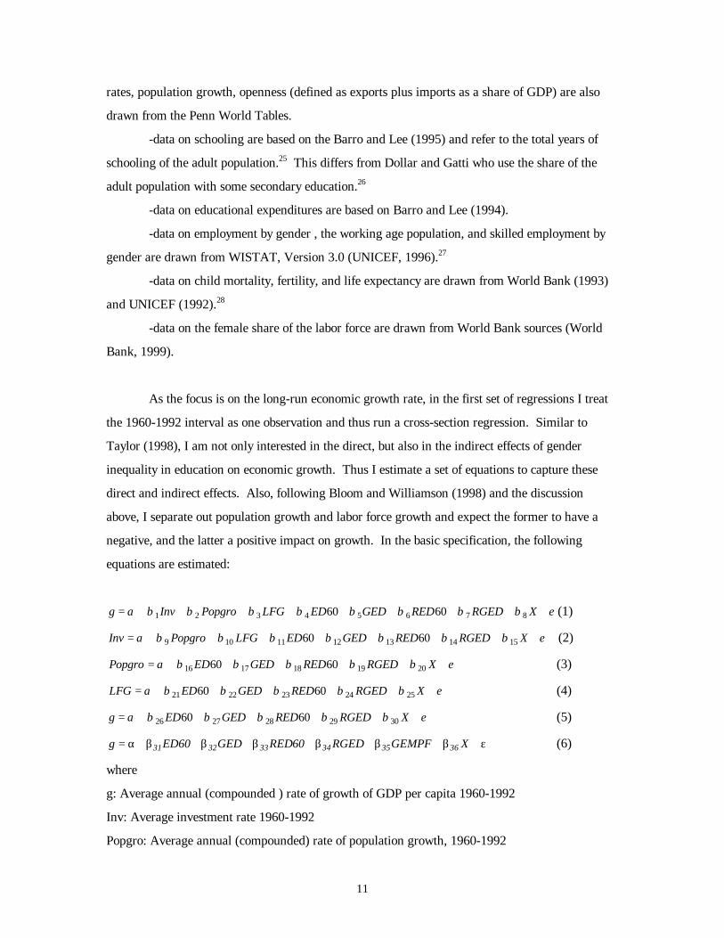
11

rates, population growth, openness (defined as exports plus imports as a share of GDP) are also

drawn from the Penn World Tables.

-data on schooling are based on the Barro and Lee (1995) and refer to the total years of

schooling of the adult population.25 This differs from Dollar and Gatti who use the share of the

adult population with some secondary education.26

-data on educational expenditures are based on Barro and Lee (1994).

-data on employment by gender , the working age population, and skilled employment by

gender are drawn from WISTAT, Version 3.0 (UNICEF, 1996).27

-data on child mortality, fertility, and life expectancy are drawn from World Bank (1993)

and UNICEF (1992).28

-data on the female share of the labor force are drawn from World Bank sources (World

Bank, 1999).

As the focus is on the long-run economic growth rate, in the first set of regressions I treat

the 1960-1992 interval as one observation and thus run a cross-section regression. Similar to

Taylor (1998), I am not only interested in the direct, but also in the indirect effects of gender

inequality in education on economic growth. Thus I estimate a set of equations to capture these

direct and indirect effects. Also, following Bloom and Williamson (1998) and the discussion

above, I separate out population growth and labor force growth and expect the former to have a

negative, and the latter a positive impact on growth. In the basic specification, the following

equations are estimated:

g Inv Popgro LFG ED GED RED RGED X= + + + + + + + + +α β β β β β β β β ε1 2 3 4 5 6 7 860 60 (1)

Inv Popgro LFG ED GED RED RGED X= + + + + + + + +α β β β β β β β ε9 10 11 12 13 14 1560 60 (2)

Popgro ED GED RED RGED X= + + + + + +α β β β β β ε16 17 18 19 2060 60 (3)

LFG ED GED RED RGED X= + + + + + +α β β β β β ε21 22 23 24 2560 60 (4)

g ED GED RED RGED X= + + + + + +α β β β β β ε26 27 28 29 3060 60 (5)

ε+β+β+β+β+β+β+α= XGEMPFRGED60REDGED60EDg 363534333231 (6)

where

g: Average annual (compounded ) rate of growth of GDP per capita 1960-1992

Inv: Average investment rate 1960-1992

Popgro: Average annual (compounded) rate of population growth, 1960-1992

12

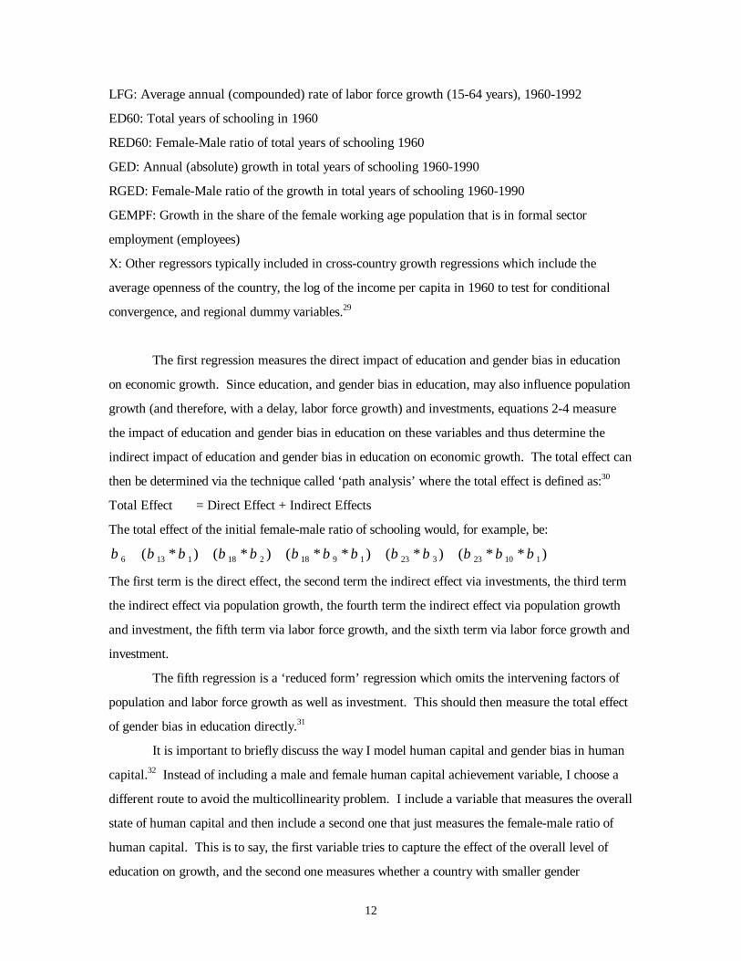
LFG: Average annual (compounded) rate of labor force growth (15-64 years), 1960-1992

ED60: Total years of schooling in 1960

RED60: Female-Male ratio of total years of schooling 1960

GED: Annual (absolute) growth in total years of schooling 1960-1990

RGED: Female-Male ratio of the growth in total years of schooling 1960-1990

GEMPF: Growth in the share of the female working age population that is in formal sector

employment (employees)

X: Other regressors typically included in cross-country growth regressions which include the

average openness of the country, the log of the income per capita in 1960 to test for conditional

convergence, and regional dummy variables.29

The first regression measures the direct impact of education and gender bias in education

on economic growth. Since education, and gender bias in education, may also influence population

growth (and therefore, with a delay, labor force growth) and investments, equations 2-4 measure

the impact of education and gender bias in education on these variables and thus determine the

indirect impact of education and gender bias in education on economic growth. The total effect can

then be determined via the technique called ‘path analysis’ where the total effect is defined as:30

Total Effect = Direct Effect + Indirect Effects

The total effect of the initial female-male ratio of schooling would, for example, be:

β β β β β β β β β β β β β6 13 1 18 2 18 9 1 23 3 23 10 1+ + + + +( * ) ( * ) ( * * ) ( * ) ( * * )

The first term is the direct effect, the second term the indirect effect via investments, the third term

the indirect effect via population growth, the fourth term the indirect effect via population growth

and investment, the fifth term via labor force growth, and the sixth term via labor force growth and

investment.

The fifth regression is a ‘reduced form’ regression which omits the intervening factors of

population and labor force growth as well as investment. This should then measure the total effect

of gender bias in education directly.31

It is important to briefly discuss the way I model human capital and gender bias in human

capital.32 Instead of including a male and female human capital achievement variable, I choose a

different route to avoid the multicollinearity problem. I include a variable that measures the overall

state of human capital and then include a second one that just measures the female-male ratio of

human capital. This is to say, the first variable tries to capture the effect of the overall level of

education on growth, and the second one measures whether a country with smaller gender

13

differences in education would grow faster than a country with identical average human capital but

greater inequality in its distribution.

There are two ways one can assess the impact of gender inequality in education. In one,

one assumes that gender inequality in education could have been reduced without reducing male

education levels. To measure this, one simply uses the male years of schooling as the measure for

average human capital. This will generate an upper level estimate of the measured impact of gender

inequality on education. In another, one assumes that any increase in female schooling would have,

ceteris paribus, led to a commensurate decrease in male schooling, which will naturally reduce the

measured effect of gender inequality and will thus represent a lower bound of the measured impact

of gender inequality in education. To generate this lower bound estimate, one includes average

years of schooling of males and females. Clearly, the true effect is likely to be between these two

estimates, probably closer to the former than the latter. I report on both specifications below.33

A second issue relates to possible simultaneity problems. As the estimation not only relies

on initial level and gender differential in human capital (ED60 and RED60), but also the growth of

educational attainment (GED and RGED), it could theoretically be the case that the causality runs

from growth to schooling (and reduced gender bias in schooling, see Dollar and Gatti, 1999), and

not the other way around as suggested here.

I try to address this issue using three different procedures. First, total years of schooling

of the adult population is a stock measure of education that is based on past investments in

education. The growth in total years of schooling of the adult population between 1960 and 1990

is largely based on educational investments that took place between 1940 and 1975. Thus it is

unlikely (but not impossible) that these investments were mainly driven by high economic growth

between 1960 and 1990.34

Second, I use instrumental variable techniques to address this issue. In particular, I use

educational spending (as a share of GDP), initial fertility levels, and the change in the total fertility

rate as instruments for changes in the educational attainment and the female-male ratio of those

changes to explicitly control for possible simultaneity. These instruments pass standard relevance

and overidentification tests and thus appear to be plausible candidates.35

Third, I re-estimate the model using a panel data set where I split the dependent and

independent variables into three time periods (1960-70, 1970-80, and 1980-90). In these panel

regressions, I only use initial values of gender gaps in education as explanatory variables. Based

on specification tests, it turns out that the best panel regression specification is to use regional and

decadal dummies, but no country specific fixed effects (nor random effects).36

14

It is considerably more difficult to find an adequate measure for inequality in access to

employment that can be used in a cross-country regression. I use two such measures and add them

to the reduced form regression 5. The first is the growth of female formal sector employment

(employees), as a share of the total number of females of working age (GEMPF in regression 6).

This variable thus seeks to capture to what extent women have been able to increase their

participation in the formal economy. The advantage of this measure is its focus on the formal

economy that may be able to capture the effect of women’s work becoming visible in the formal

economy. At the same time, measurement error and international compatibility of these data is

likely to be an issue. Also, there is a potential simultaneity issue.37 Moreover, the data is only

available for some 65 countries. The second measure is the change in the share of the total labor

force that is female. This information is available for more countries, but also suffers from

measurement, compatibility, and simultaneity issues.

I estimate these models for a sample of 109 countries, which include industrialized and

developing economies. I also perform the same analysis on a subsample of only developing

countries and on a sample that only includes African economies to see whether this relationship

differs between different regions.38

B. Fertility and Child Mortality Regressions

I also estimate models of fertility and child mortality. These models estimate the levels of

child mortality and fertility in 1990 and also examine the direct and indirect impact of education

and gender inequality in education, using the same procedures as described above.

V. Growth, Schooling, and Gender Inequality

This section presents some regional averages on growth, its most important determinants,

as well as gender inequality in education and employment. These data form the background for the

multivariate analysis performed in the next section.

Table 1 shows that annual growth in per capita incomes between 1960 and 1992 was

slowest in Sub-Saharan Africa, averaging only 0.7% per year. This is about one-third of the world

average, and fully 3.5% slower (per year !) than in East Asia and the Pacific. Growth in Latin

America was also very slow, followed closely by South Asia. Similarly, average rates of

investments were very low in Africa, although they remained slightly above those in South Asia.

Finally, Africa and South Asia are the two regions with the highest under five mortality, and,

together with the Middle East and North Africa, the highest fertility levels. Clearly, these are the

regions where well-being is lowest.

15

Moreover, Africa, South Asia, and the Middle East and North Africa suffered from a

number of disadvantages in initial conditions. Table 1 shows that under five mortality in 1960 and

population growth between 1960 and 1992 were highest in these three regions. In Africa, the

average number of total years of schooling for the female adult population (aged 15 or older) in

1960 was at a dismal 1.09 years, only surpassed by even lower female educational attainment rates

in South Asia and equally poor rates in the Middle East and North Africa. Gender inequality in

schooling in 1960 was also very high in Africa, with the women haven barely half the schooling of

men. South Asia and the Middle East had even worse differentials.

Particularly worrying is that females in Africa have experienced the lowest average annual

growth in total years of schooling between 1960 and 1990 of all regions (an annual increase of only

0.04 years increasing the average years of schooling of the adult female population by a mere 1.2

years between 1960 and 1990). Moreover, the female-male ratio in the growth of total years of

schooling is 0.89, meaning that females experienced a slower expansion in educational achievement

than males. Also here, South Asia and the Middle East and North Africa are equally poor

performers. While overall education levels expanded much faster than in Africa, females lagged

even further behind than males in the expansion of education. The contrast with East Asia is,

again, striking. There female years of schooling expanded at three times the speed of Africa, and

female expansion outpaced male expansion of education by 44%.

Finally, females in Africa, South Asia, and the Middle East have a weak position in the

formal labor market. In 1970, the female-male ratio of formal sector employment was among the

lowest in the developing world, and the share of women in professional, technical, administrative,

and managerial workers was also very low. Apart from a weak initial position, there have been

only minor improvements in the employment opportunities of women. The share of female formal

sector employment (employees as a share of the working age population) increased in Africa by

only 1.6 percentage points between 1970 and 1990. Only South Asia had an even lower growth

rate, while all other regions had much higher rates of female formal sector employment growth.

Also, the share of females in the labor force stagnated in Africa while it rose considerably

everywhere else.

Thus Africa, together with South Asia and the Middle East, seems to suffer from the worst

initial conditions for female education and employment as well as the worst record of changes in

female education and employment in the past 30 years. In contrast, East Asia and the Pacific

started out with better conditions for women’s education and employment. More importantly,

16

however, females were able to improve their education and employment opportunities much faster

than men, thereby rapidly closing the initial gaps.39

At the same time, Africa’s and South Asia’s initial incomes were the lowest of the world in

1960 which should have helped boost growth rates, as trade and factor flows should promote

convergence of income levels. Africa’s economies experienced average levels of openness, while

South Asia’s economies appeared more closed. This is slightly deceptive, however, since one

would have expected the many small economies of Africa to have above average levels of openness

due to the limited size of their domestic markets. Compared to East Asia, Africa’s economies were

much less open.

If gender inequality in education has an impact on economic growth, I would therefore

expect South Asia, Sub-Saharan Africa, and the Middle East to have suffered the most as they

experienced the largest initial gender inequality in education as well as the largest gender inequality

in the expansion of education while I would expect East Asia and Eastern Europe to have benefited

from lower inequality in education.

VI. Multivariate Analysis of the Impact of Gender Inequality on Economic Growth

A. Growth Regressions

Table 2 shows the basic regression equations (1) through (6) as described above. All

regressions have a high explanatory power and perform well on on specification tests. Regression

(1) confirms a number of known findings regarding conditional convergence (LNINC1960), the

importance of investment and openness for growth (INV, OPEN), the importance of initial levels of

human capital (ED60) as well as growth in human capital (GED), the negative impact of

population growth and the positive impact of labor force growth (POPGRO, LFG, e.g. Barro,

1991; Bloom and Williamson, 1998; ADB, 1997, Mankiw, Roemer, and Weil, 1992). The size of

the coefficients on these variables are within the range of values observed in other studies. Some of

the dummy variables for the various regions are significant (esp. those for Africa and Latin

America) suggesting that the growth regression is not picking up all effects that account for slower

growth in these two regions (see also Barro, 1991).40

More interesting for our purposes is the finding that both the initial female-male ratio of

schooling achievements (RED60) as well as the female-male ratio of expansions in the level of

schooling (RGED) has a significant positive impact on economic growth. Since I control for both

investment as well as population and labor force growth, these results provide some support for the

selection/distortion effect of gender bias in education as well as the ‘direct’ externality effect where

17

lower gender inequality in education is associated with higher quality of education. The magnitude

of the coefficient is also within the range of the possible. An increase in the female-male ratio of

growth in schooling from 0.5 to 1.0 would raise the annual growth rate by about 0.4% (see also

below).

Empirically, gender inequality in education also appears to be related to the health of the

population. When I include the under five mortality rate in 1960 or life expectancy in 1960 in the

regressions (not shown here), the direct effects of gender inequality in education on growth become

smaller (but remain sizable), and the coefficients on child mortality and longevity are in the right

direction, but not significant. As I show below that lower gender inequality in education seems to

lower child mortality, this suggests that a third way lower gender inequality in education is

promoting economic growth is through the effect it has on lowering child mortality and thus

improving the health of the population.41

Regression 2 shows the determinants of investments and finds that higher investment rates

are related to higher labor force growth, greater openness, and higher human capital. In addition,

reduced gender inequality in education also appears to lead to higher investment rates, confirming

the indirect linkage between gender inequality in education, investment, and economic growth

postulated above. In particular, initial gender gaps in education appears to negatively affect

investment rates.

Regressions 3 and 4 also show that gender inequality in education has the expected impact

on population growth and labor force growth so that the indirect linkage between gender inequality

in education and economic growth via these two factors is also present.

Regression 5 then shows the ‘reduced form’ estimate of the impact of gender inequality in

education. Comparisons between regressions 1 and 5 indicate that the indirect effects of gender

inequality in education are indeed sizable as the size (and significance) of both coefficients, but

particularly the one relating to initial gender inequality, have increased considerably. This suggests

that the initial level of gender inequality mainly affects growth indirectly, particularly through the

impact it has on investment rates.

In regressions 6 and 7, I add two possible measures of gender bias in employment to

determine their effect on economic growth. The first one, the growth in the female share of the

working age population that is employed in the formal sector has a large and significant impact on

economic growth, while the other one, the growth in the female share of the labor force, also has a

positive but insignificant impact on economic growth. These results should be treated with some

caution. While they may be related to the selection effect and the measurement effect described

18

above and thus show how greater access to employment for females boosts economic growth, it is

also possible that the causality runs from economic growth to drawing females into the labor force.

Given the poor data on women’s employment and wages, I am unable to come up with a good

instrument that could address this issue. Thus the results on employment inequality remain

suggestive and do indeed point to a possible effect of reduced gender inequality in employment on

economic growth.42

In Table 3, I use the results from regressions 1-5 to determine to what extent growth in

South Asia and Sub-Saharan Africa lagged behind growth in East Asia due to initial gender bias in

education and gender bias in the growth of education. The numbers refer to the combined effect of

initial gender gaps in education and gender gaps in the growth of education. In parentheses, I

include the figures for the impact of the initial gender gap in 1960 and the gender gap in the growth

of education, respectively. Using just the direct effect (regression 1) 0.45% of the annual growth

difference of 3.5% between Africa and East Asia can be accounted for by differences in gender

inequality in education, where most of the difference is due to differences in the gender bias in the

growth of education. The comparison between South Asia and East Asia is even more striking.

Fully 0.69% of the annual growth difference of 2.5% can be accounted for by differences in gender

inequality in education;43 here, about 2/3 of the difference can be accounted for by differences in

gender bias in the growth of education, while 1/3 are due to differences in levels of gender

inequality in 1960. Similarly, gender inequality in education appears to have slowed growth in the

Middle East and North Africa by similar amounts to the ones observed in South Asia.

In addition to the direct effects, the indirect effects can also account for some of the growth

differences between South Asia (Africa) and East Asia. Gender inequality in education can, via the

effect on investment, account for a further 0.16% of the growth difference between South Asia and

East Asia (0.07% of the difference Africa-East Asia). Gender inequality in education also

accounts for 0.13% of the growth difference between South Asia and East Asia via the impact on

population growth (0.09% of the difference Africa East Asia). These indirect effects, esp. the one

operating via the population and labor force growth rates, are somewhat smaller than expected.

Unless this is due to data issues, this suggests that the indirect effect, while present and significant,

is of smaller magnitude than the direct distortionary effect of closing educational opportunities for

promising female students and of reducing the positive externality of educated females on the

quality of education of other household members.

The total direct and indirect effects of gender inequality in education account for about

0.95% of the growth difference between South Asia and East Asia, about 0.56% of the growth

19

difference between Sub-Saharan Africa and East Asia and about 0.85% between the Middle East

and North Africa and East Asia. Since the initial level of gender inequality plays a larger role in

the indirect effects than in the direct effect of gender inequality on economic growth, the total

impact of gender inequality in education on growth differences between Africa and East Asia (East

Asia and South Asia) is due to 1/3 (55%) to gender differentials in 1960, and 2/3 (45%) due to

gender differentials in the growth of education. Using the reduced form regression (regression 5)

yields virtually identical estimates of the total size of the effects as well as their impact on the

growth differences between developing regions (Table 3).

Thus gender inequality in education appears to have a sizable effect on economic growth.

It is important to emphasize that the results in Table 3 do not take into account the differences in

average human capital between the regions, but just the gender inequality in education. From the

regressions, it can be seen that differences in average human capital also matter a lot and can

account for a further share of the growth differences between the developing regions.

Based on regression 6, I also incorporate the effect of employment inequality on economic

growth and find that it could account for about another 0.3% of the growth difference between East

Asia and South Asia, Sub Saharan Africa, and the Middle East, respectively.

As discussed above, it is important to determine the robustness of the results presented

above. First, it was mentioned above that the estimates on gender inequality in education present

an upper bound estimate as they implicitly assume that increases in female education could, ceteris

paribus, have been achieved at no reduction in male educational enrollments. In columns (8) and

(9) in Table 4, I present the regressions for the lower bound estimate,44 where I use the average

level of human capital rather than the male level of human capital used above.

As to be expected, the size of the coefficients on the gender gap in schooling is now

smaller, but still sizable and, in most cases, significant. Calculations of the growth differences

accounted for by this measure of gender inequality in education shows only small differences to the

previous one (Table 3). Now the total effect of gender inequality in education can account for

0.77% of the growth difference between South and East Asia, 0.44% of the difference between

Sub-Saharan Africa and East Asia, and nearly 0.7% of the difference between East Asia and the

Middle East. Adding the measure for employment inequality can again account for about another

0.3% of the growth differences.

Second, I need to worry about possible simultaneity issues; in particular, can it be the case

that growth led to increases in the female-male ratio of schooling attainment rather than the other

way around?

20

Regressions 10 and 11 are based on a panel analysis where the dependent and independent

variables are split into three different time periods. As I only include initial levels of schooling and

the initial female-male ratio of schooling in the regression, I avoid the simultaneity issue inherent in

the educational growth variables. The results are very similar to the cross-section results which is

very reassuring as often findings from cross-country regressions change in a panel setting. In fact,

even the magnitude of the effects appears to be roughly similar to the cross-section regression. In

Table 5, I estimate the impact of gender inequality in education using the panel regressions.45 In

the 1980s, in initial gender inequality in education accounted for some 0.3-0.5% of the growth

differences between East Asia and the other three regions. This is smaller than found in the cross-

section regression, which is to be expected as we no longer consider the impact of further

improvements in the gender gap in education that may have occurred after 1980.

The panel regressions also show an interesting temporal pattern of the impact of gender

inequality in education on economic growth. In 1960, East Asia did not exhibit much lower gender

bias in education and the growth differences between it and the other regions were comparatively

small. By 1970 and also 1980, East Asia’s gender gap was much lower than in the other regions

and it was precisely then when growth differences really soared between East Asia o the one hand,

and South Asia, Sub Saharan Africa and the Middle East on the other. This confirms that the

timing of gender gaps in education and economic growth suggest that reduced gender gaps in

education did indeed play a significant role in furthering growth.

To approach the simultaneity issue in another way, regression 12 presents a two stage least

squares regressions where both the growth in average education and the female-male ratio of

growth in average education are replaced by their predicted values using government spending on

education, the total fertility rate in 1960, and the change in fertility rate between 1960 and 1990 as

instruments.46 Now the impact of the female-male ratio in the growth of education is still

significant and considerably larger in magnitude. This lends further support to the contention that

causality runs from gender bias in education to economic growth and not the reverse.

In further analyses, I investigate whether the relationship between gender inequality and

growth differs depending on which countries are included in the regression. While limiting the

sample to more homogeneous groups of countries has the advantage of seeing whether the effects

differ by region, it carries the disadvantage that some of the important variation that is needed to

estimate these effects is thereby eliminated which may lead to less precise results. Limiting the

sample to 85 developing countries (regression 13 shows the reduced form regression) changes the

results by very little. The impact of initial gender inequality is slightly larger than in the total

21

sample, while the impact of gender bias in the growth of education is now smaller. Using these

regressions to account for growth differences suggest that the gender inequality in education

accounts for some 0.44% of the growth difference between Africa and East Asia, and 0.81% of the

growth difference between South Asia and East Asia. Adding gender inequality in employment

adds another 0.4-0.5% (not shown).

Thus the effect of gender inequality on growth is as strong in developing countries as it is

in developed countries. This findings differs from Dollar and Gatti (1999) who found gender

inequality in education to have a significant impact only among countries with higher levels of

female education. As the econometric methodology, time period considered, and some of the

exogenous variables, including the human capital variables differ, it is not easy to determine what

drives the differences in results. One thing I was able to determine is that the difference does not

appear to come from the human capital variable used by Dollar and Gatti. When I use their human

capital variable (share of the adult population with exactly some secondary education) and an

amended version (share of the adult population with at least some secondary education), it still is

the case that gender bias hurts growth among poor and rich countries.47 Other than that, I can only

point to the fact that I consider a longer time period (32 years) in a cross-section or a three decade

panel, while Dollar and Gatti limit the analysis to 75-90 (in five-year intervals), that I model the

gender gap in education differently to avoid multicollinearity problems, and that I include a few

different independent variables (including the investment rate and population and labor force

growth) to explicitly consider direct and indirect effects.

Limiting the sample to African countries (27 observations) produces some interesting

results, as shown in regressions 14 and 15 in Table 4. Now the impact of initial gender inequality

in education is much larger and the impact of gender bias in the growth of educational attainment is

slightly larger than in the overall regression. It thus appears that gender inequality in education

appears to matter more in Africa than elsewhere. This may seem a bit surprising since one might

expect growth in the largely agricultural African societies not to depend as much on education in

general and female bias in particular. The regressions seem to suggest otherwise. They support a

view that human capital is indeed very important also in Africa’s agricultural societies. Moreover,

given the important role women play in African agriculture, their poor human capital appears to be

a particularly important constraint for economic growth.48

To estimate the impact of gender bias in education in the African context, Table 6

calculates the contribution of gender inequality in education on the growth difference between

Botswana, a country with low gender inequality in education, and Ghana and Niger, two countries

22

with high gender inequality in education. The growth differences between the three economies are

sizable, with Botswana having grown by more than 5.5%, while Ghana and Niger grew by less

than 0.3% per year between 1960 and 1992. Gender inequality in education can account for a total

of 1.59% of the growth difference between Ghana and Botswana and a total of 1.82% of the total

growth difference between Niger and Botswana. These are very large effects indeed.

B. Fertility and Child Mortality Regressions

In Table 7, I estimate models of fertility and child mortality to determine to what extent

gender bias in education might hinder progress in reducing fertility and childhood mortality rates.

Regression 16 estimates a model to predict total fertility rates in 1990. The regression reproduces

findings from many other studies about the importance of female education for fertility (e.g.

Murthi, et al. 1995; Drèze and Sen, 1995; Summers, 1994). Every year of female education

reduces the total fertility rate by 0.23, while increases in male education raise the fertility rate (as

one would expect from economic theories of the household, e.g. Becker, 1981). Higher child

mortality promotes fertility while higher incomes lower fertility, both also as expected. Regression

17 then uses the measures of human capital used previously (average achievement and the gender

gap) to make it compatible with the remaining parts of the paper. It shows that average education

makes little difference to the fertility rate, while the ratio of female to male achievement is highly

significant. This clearly demonstrates that gender bias in education prevents reductions in fertility

and thus harms women and their families in developing countries.

Also here there may be direct and indirect effects. In particular, income in 1990 (as

demonstrated above) and the under five mortality rate in 1990 may be influenced by gender gaps in

education. Therefore I need to take into account those indirect effects and estimate a reduced form

regression as well. Regression 18 shows that there is indeed a very large effect of gender bias in

education on under five mortality, which is an important finding in its own right. Even after

controlling for income, average human capital, and other regional differences, gender bias in

education has a huge impact on child mortality. If Sub Saharan Africa experienced the gender gap

in education of Eastern Europe (without experiencing their income level or their average human

capital), the under five mortality rate would be about 45/1000 lower than it currently is. Thus

gender bias in education leads to higher child mortality and thus prevents progress in this critical

development achievement (Sen, 1999).

Regression 20 then shows the reduced form regression of the fertility rate which

demonstrates the sizable impact of gender gaps in education on fertility, both directly as well as

indirectly via its impact on child mortality.

23

VII. Conclusion

This paper has examined the question to what extent gender inequality, particularly gender

inequality in education and employment reduces growth and development. It may be useful to

briefly highlight the most important findings:

First, it appears that gender inequality in education does impede economic growth. It does

so directly through distorting incentives and indirectly through its impact on investment and

population growth. The effects are sizable. Had South Asia and Sub-Saharan Africa found

themselves with more balanced educational achievements in 1960, and had they done more to

promote gender-balanced growth in education, their economic growth could have been up to 0.9%

per year faster than it turned out to be the case.

Second, these effects do not appear to be related to simultaneity issues. Several

specifications, and the use of instrumental variable estimation show that the effect of gender

inequality in education on economic growth persists.

Third, it appears that the effect is stronger in Sub Saharan Africa. Promoting female

education appears to therefore have a higher payoff there than elsewhere.

Fourth, gender bias in employment is also associated with lower growth although here

measurement and causality issues are harder to sort out. Gender inequality in employment in South

Asia and Sub-Saharan Africa may have reduced growth by another 0.3%, compared to East Asia.

Fifth, gender inequality in education has large and significant effects on fertility and child

mortality. Since reduced fertility and child mortality (and, conversely, expanded longevity) are

among the most important constituent elements of well-being (Sen, 1999), these findings may be at

least as relevant for the well-being of people in developing countries as the findings regarding

economic growth (which is just one means to generate greater well-being).

In fact, it appears that promoting gender equity in education and employment may be one

of those few policies that have been termed ‘win-win’ strategies. It would further economic

prosperity and efficiency, promote other critical human development goals such as lower mortality

and fertility, and it would be intrinsically valuable as well.

It may be important to end this investigation with some cautionary notes. As with all

empirical growth regressions, the results show associations but cannot prove causality. While the

results presented here do indeed suggest a strong linkage between gender inequality and economic

growth, fertility, and child mortality, it is possible that these findings are due to the omission of

some variable that is related to both outcomes, that measurement errors affect the results, or that

24

the model is misspecified in other ways. Only further investigations of this nature, as well as

complementary analyses using micro data will be able to conclusively determine the importance of

the linkages explored here.

References

Asian Development Bank. 1997. Emerging Asia. Manila: ADB.

Baliga, S. S. Goyal, and S. Klasen. 1999. Education and Marriage Age: Theory and Evidence.University of Munich Discussion Paper. Munich: Department of Economics.

Becker, G. 1981. A Treatise on the Family. Chicago: University of Chicago Press.

Bardhan, Kalpana and Stephan Klasen. 1999. UNDP’s Gender-Related Indices: A CriticalReview. World Development 27: 985-1010.

------. Gender in Emerging Asia. 1997. Background paper for Asian Development Bank BookEmerging Asia. Manila: ADB.

Barro, R. 1991. Economic Growth in a Cross-Section of Countries. Quarterly Journal ofEconomics 106: 407-443.

-------. and J. Lee. 1995. International Measures of Educational Achievement. AmericanEconomic Review 86: 218-223.

------. 1994. Sources of Economic Growth. Carnegie-Rochester Series on Public Policy.

Barro, R. and X. Sala-i-Martin. 1995. Economic Growth. New York: McGraw-Hill.

Bloom, D. and J. Williamson. 1997. Demographic Transition and Economic Miracles inEmerging Asia. NBER Working Paper 6268.

Bruno, M., L. Squire, and M. Ravallion. 1996. Equity and Growth in Developing Countries.Policy Research Working Paper No. 1563. Washington DC: The World Bank.

Collier, P. and J Gunning. 1998. Explaining African Economic Performance. Mimeographed.Washington DC: The World Bank.

Dollar, D. and R. Gatti. 1999. Gender Inequality, Income, and Growth: Are Good Times good forWomen? Mimeographed. Washington DC: The World Bank.

Drèze, Jean and Amartya Sen. 1995. India Economic Development and Social Opportunity. NewYork: Oxford University Press.

-----. 1989. Hunger and Public Action. New York: Oxford University Press.

Easterly, B. and R. Levine. 1997. Africa’s Growth Tragedy: Policies and Ethnic Divisions.Quarterly Journal of Economics 92: 1203-50.

25

Heston, A. and R. Summers. 1991. ‘The Penn World Table Mark 5’. Quarterly Journal ofEconomics 106: 328-368

King, E. and A. Hill. 1995. Women’s Education in Development Countries. Baltimore: JohnsHopkins Press.

Klasen, S. 1994. ‘Missing Women Reconsidered’. World Development 22: 1061-71.

------. 1993. Human Development and Women’s Lives in a Restructured Eastern Bloc, in Schipke,A. and A. Taylor (eds.) The Economics of Transition: Theory and Practise in the New MarketEconomies. New York: Springer.

Lagerlöf, N. 1999. ‘Gender Inequality, Fertility, and Growth’. Mimeographed. Department ofEconomics, University of Sydney.

Lucas, R. 1988. On the Mechanics of Development Planning. Journal of Monetary Economics22: 3-42.

Mankiw, N.G., D. Roemer, and D. Weil. 1992. A Contribution to the Empirics of EconomicGrowth. Quarterly Journal of Economics 107: 407-437.

Murthi, M., Guio, and J. Drèze. 1995. Mortality, Fertility, and Gender Bias in India: A District-Level Analysis. Population and Development Review 21: 745-782.

NBER. 1998. The Penn World Tables Mark 5.6. Cambridge, MA: WWW.NBER.ORG.

Palmer., I. 1991. Gender and Population in the Adjustment of African Economies. Geneva: ILO.

Pritchett, L. and L. Summers. 1996. ‘Wealthier is healthier.’ Journal of Human Resources31:841-868.

Roemer, P. 1986. Increasing Returns and Long-Run Growth. Journal of Political Economy 94:1002-1037.

Sato, K. Raising the Productivity of Women Farmers in Sub-Saharan Africa. World BankDiscussion Paper No 230.

Sachs, J. and M. Warner. 1997. Source of Slow Growth in African Economies. Journal ofAfrican Economies. 6: 335-76.

-------. 1995. Natural Resources and Economic Growth. Development Discussion Paper 517a.Harvard Institute for International Development.

Schultz, T.P. 1993. Changing World Prices, Women’s Wages, and the Fertility Transition inSweden, Journal of Political Economy 101: 1126-1154.

Seguino, S. 1998. Gender Inequality and Economic Growth: A Cross-Country Analysis.Mimeographed. University of Vermont.

26

Sen, Amartya. 1999. Development as Freedom New York: Knopf (forthcoming).

------. 1990. Gender and Cooperative Conflicts, in Tinker, Irene (ed.) Persistent Inequalities(Oxford: Oxford University Press).

------. 1989. Women’s Survival as a Development Problem. Bulletin of the American Academy ofArts and Sciences 43: 14-29.

Solow, R. 1956. A Contribution to the Theory of Economic Growth. Quarterly Journal ofEconomics 70: 65-94.

Summers, L. 1994. Investing in All the People. Washington DC: The World Bank.

Taylor, Alan. 1998. ‘On the costs of inward-looking development.’ Journal of Economic History58: 1-28.

Thomas, D. 1990. Intrahousehold Resource Allocation: An Inferential Approach. Journal ofHuman Resources 25:634-64.

UNDP. 1995, 1996. Human Development Report. Various Issues. New York: Oxford UniversityPress.

UNICEF. 1996. Women’s Indicators and Statistics (WISTAT), Version 3.0. New York: UNICEF.

UNICEF. 1992. The State of the World’s Children. New York: UNICEF.

Waring, M. 1988. If Women Counted. New York: Harper and Row.

Wold, B. 1997. Supply Response in a Gender-Perspective. Mimeographed. Oslo: StatisticsNorway.

World Bank. 1999. World Development Indicators. Washington DC: The World Bank.

-----. 1993. World Development Report. New York: Oxford University Press.

Young, Alwyn. 1995. ‘The Tyranny of Numbers: Accounting for the Economic Miracle in EastAsia’. Quarterly Journal of Economics, 641-680.

27

1 This has, for example, been recognized in the creation of UNDP’s Gender-Related Development Indexwhich, derived from a notion of aversion to inequality, suggests that a country with higher genderinequality achieves a lower level of aggregate well-being compared to another with equal averageachievements, but lower gender gaps (UNDP, 1995). Unfortunately, the way the index is constructed isopen to serious criticisms. For a discussion, see Bardhan and Klasen (1999).2 The basic theoretical question is whether human and physical capital combined still exhibit diminishingreturns, or whether they together exhibit constant returns. In the framework of a Cobb-Douglasproduction function, the question thus becomes whether the exponents on physical and human capital sumto 1 (endogenous growth) or to less than one (conditional convergence).3 The model assumes that parents aim to maximize the household incomes of their children. If gendergaps in education between the sexes exist, it may be optimal for parents to also concentrate educationalinvestments on sons as daughters are likely to marry an educated male, while sons are likely to marry anuneducated women These self-perpetuating gender gaps in education lead to high ferility as theopportunity cost of time for uneducatd women is low. High fertility will mean low investments in eachchild which can force an economy to remain in a poverty trap. Public action to reduce the gender gap canbreak this self-perpetuating cycle and help the economy break out of a poverty trap. For details, seeLagerlöf (1999).4 This procedure can be done using OLS and yields consistent estimates as the system of equations that isbeing estimated is recursive, not simultaneous. Thus one can first consistently estimate the structuralequations determining the endogeous variables then estimate the growth regression using thoseendogenous variables. Care must be taken, however, in interpreting the results, as one has to distinguishbetween direct and indirect effects.5 In addition, some variables may influence economic growth only through the impact they have on thestructural parameters. Taylor (1998) finds, for example, that government spending affects growth of GDPnot directly, but only through its impact on investment.6 At the same time, the speed of convergence is slower than predicted in the standard Solow model. In aSolow model augmented by human capital, the speed of convergence is predicted to be much slower andmore in line with actual observations (Mankiw, Roemer, and Weil, 1992).7 For example, it is difficult to distinguish empirically whether the observed association between theinvestment rate and economic growth is due to transitions from one steady state to another (as it would inthe Solow model) or due to a permanent increase in the growth potential of the economy due to this higherinvestment (as in an endogenous growth framework).8 For example, one may wonder whether the combination of being landlocked and having little access tothe coast and being located in the tropics, as used by ADB (1997) and Sachs and Warner (1997) is simplyanother description for low-growth Africa and does therefore not necessarily ‘explain’ Africa’s pooreconomic performance.9 I am able to replicate Barro’s results with the data used here but indeed find multicollinearity to be a bigproblem. Dollar and Gatti (1999) find that Barro’s results disappar as soon as one introduces a dummyvariable for Latin America.10 In particular, they use religion and civil liberty variables as instruments for explaining male and femaleeducational achievement. This would work if both of these variables are uncorrelated with economicgrowth. The latter, however, has been used in a variety of growth regressions and does indeed appear tobe associated with economic growth (Taylor, 1998; Sachs and Warner, 1995).11 In other continents, this effect is even larger.12 Many of these studies do not examine gender inequality in education directly, but focus on the impact offemale education. For example, Murthi et al, 1995 examine the impact of female and male literacyseparately and find female literacy to have a strong negative impact on fertility while male literacy has noimpact. Some studies have even found that male literacy has a positive impact on fertility while femaleliteracy has a negative one.13 For example, in a study for the Asian Development Bank, Sachs, Radelet, and Lee have found that highpopulation growth depressed per-capita growth in Sub-Saharan Africa by 0.7% per year between 1965 and1990; this factor alone accounted for about 15% of the difference in growth performance between Sub-Saharan Africa and South-East Asia (ADB, 1997). Similarly, Bloom and Williamson (1998) find that the

28

early fertility transition in East and South-East Asia is an important contributing factor in accounting forEast Asia’s economic miracle.14 The same might be true, to a lesser extent, for growth regressions including child mortality or lifeexpectancy.15 The calculations assume that innate abililities are normally distributed and compares two possibledistributions of the student population. In one, 50% of an age cohort get educated and helf are male andhalf are female. In the other, 50% get educated and 70% are male and 30% are female. It turns out thatthe average human capital (which is defined simply as the Z-score of the standardized normal distributionmultiplied by the 0-1 variable for getting educated) would be some 12% lower in the second scenario.Using the regression coefficient from Mankiw, Roemer, and Weil (1992) would yield some 0.3%difference in annual growth.16 Even if people have a preference for marrying someone with similar education levels (as appears to bethe case), gender inequality in education will force the marriage of educated men with uneducated femalesand thus may prevent the spillover from taking place. For a discussion of these and related issues, seeBaliga et al. (1999).17 It is difficult to quantify the potential impact of this externality.18 The following calculation illustrates the point. If 100 workers have to care for 100 dependants, thentheir average wage of $1000 a year will translate into $500 per capita income ((100*$1000)/200). If,however, 150 workers have to care for only 50 dependants, then the average wage of $1000 a year willtranslate into $750 per capita income ((150*$1000)/200).19 Finally, gender inequality in education may hamper growth through its impact on child health. Bettereducated females have healthier children, which has been found to increase growth in the long run(Summers, 1994, ADB, 1997). These effects will only appear with some lags and are therefore often quitedifficult to measure.20 This contrasts with the arguments advanced by Seguino (1999) who argues that gender discriminationin the labour market will favour growth as it will lead to lower female wages in export-intensive sectors.The argument advanced differs from this by focusing on access to employment rather than wages. Iffemales do not have access to employment, then labor supply is artificially restricted and men will earnhigher wages, making the country less competitive.21 This effect can become very large if, for example, previous housewives decide to go into the formaleconomy and then hire a person to do the housework. Then not only women’s labor in the economy, butalso their previously unrecorded housework has become visible and will contribute to GDP.22 It is, however, not clear that one can always assume this to be the case. For example, one can imaginescenarios where reduced gender inequality increases women’s SNA activities and may reduce their non-SNA activity, thereby having a smaller than observed impact on total economic product (this may, forexample, be the case, if women enter the labor force and hire child care for their children; both increasesmeasured output, although the hired childcare is simply replacing previously unrecorded childcareactivities). The impact of this effect in accounting for East Asian growth was already discussed.23 I do not have data for all countries in 1960 or up until 1992. Thus for some countries, the time intervalconsidered is shorter. This is taken into account in the calculation of average growth rates of all thevariables.24 This is in contrast to using an uncompounded growth rate, where one would simply divide the final yearincome by the initial year income times the number of years of the interval as used by ADB (1997) forexample. The advantage of using the compounded growth rate is that this is actually how growth ismeasured year on year.25 For the regressions using data on initial schooling in 1960, adult is defined as age 15 or older. For thepanel regressions and the comparisons with Dollar and Gatti, adult is defined as 25 or older. The resultsdo not differ much by the choice of this cut-off.26 There are advantages and disadvantages in each type of variable. The advantage of using total years ofschooling is that it captures the average length of the entire educational career of the adult population,while the other measure does not, for example, differentiate between those with no education and completeprimary (both are counted as having no secondary). On the other hand, total years of schooling(implicitly) imposes the restriction everyone achieved this average figures and that differences in years ofschooling between people do not matter. The other measure takes, to a limited degree, such differences

29

into account. The particular measure used by Dollar and Gatti, the share of the adult population that hasexactly achieved some secondary education (as their highest achievement) is a bit peculiar as it excludespeople who have achieved more than complete secondary education. In some countries where the a largeshare of adults have more than secondary education (such as the US or Canada), this measure will showstagnation as the share of the population who terminated their education with some secondary schooling isstangnat and may soon fall. It would be preferable to use a measure that counts all people who have atleast some secondary education, which Dollar and Gatti do in some of their specifications.27 The data for the working age population only run from 1970 to 1994. I therefore also compared thedata to sources from the World Bank and they did not change the results.28 I also compared the data from the used sources with other data and found generally similar results. Forexample, I compared data on terms of trade from Barro and Lee with data from the World Bank on thesame issue. Similarly, I compared the WISTAT data on working age population with similar data fromthe World Bank, and compared life expectancy data from the World Bank (1993) with those fromUNICEF. In general, the regressions were not significantly altered by the use of any of these differentdata sources.29 I also used a variety of policy variables, such as government consumption, quality of institutions, andothers. Although some were significant, they added little to the explanatory power of the regressions andwere omitted in the final specification used here.30 An important assumption in interpreting such a path analysis is that one has good reason to believe thatthe causality in the indirect regressions runs from gender bias in education to investment, populationgrowth, and labour force growth. In these three cases it seems to be the case, which is the reason whyonly these three indirect effects are considered here.31 The coefficients on the reduced form regressions should measure the total effect exactly, and thus justreproduce the results that have already been arrived at through regressions 1-4. But since regression 2-4does not use all regressors from regression 1 (as I are only trying to determine important causal linkages),I do not expect the calculations of the total effect and that arrived at by the reduced form regressions to beidentical.32 An important issue to raise is the question whether a stock or flow measure of human capital is moreappropriate for such an estimation. As I am trying to model economic growth, it appears appropriate tofocus on flow measures such as physical and human capital investments and thus use the change in yearsof schooling as a proxy for investments in human capital. At the same time, it may be the case that, due toexternalities and complementarities between factors of production, the stock of human capital increasesthe growth of the economy as it makes physical capital more productive. Therefore it is useful to includeboth a stock as well as a flow measure as I propose for the regressions.33 Another way to model gender inequality in education would be to have a variable for male educationand then a second one for the difference between female and male education. It turns out that the resultsare very similar to using ratios.34 In regression not reported here, I also estimated a different specification where I replace ED60, RED60,GED, and RGED with ED75 and RED75, which is the total years of schooling of the adult population (25or older) in 1975. It is not possible for this measure of human capital to have been greatly influenced byeconomic growth since the investments (esp. those in primary and secondary education) necessary togenerate the total years of schooling of the population above 25 in 1970 were virtually all done between1930 and 1960 and cannot therefore have been influenced by economic growth since 1960.35 The instruments are much better at predicting the female-male ratio of growth in education than to themale growth in education (where they only hava a weakly significant impact). They pass theoveridentification restriction test with ease.36 The Breusch-Pagan test suggests that there is no reason to believe that there are random or fixed effects.Moreover, a fixed regression specification in a panel with only three time series observations often leads toinconsistent results. The specification with regional and decadal dummies has the highest explanatorypower and easily passes the Ramsey Reset test for omitted variables. The fixed and random effectsspecifications yield qualitatively the same results.37 Growth may draw women as much into the formal labour force as that their formal participationgenerates economic growth.

30

38 All standard errors are adjusted for heteroscedasticity and I use the Ramsey Reset test to investigate thepresence of omitted variables.39 Eastern Europe is also notable for its small gender gaps in education and employment. For adiscussion, see Klasen (1993).40 Inclusion of geographical factors, as done in ADB (1997) would reduce the size and significance of thedummy variables. It is not clear, however, to what extent these geographical variables are able to explainthe slower growth in these regions rather than simply provide another way of describing this fact.41 This also suggests that the inclusion of initial life expectancy in growth regressions (e.g. ADB, 1997) ispartially picking up this effect which is really due to gender inequality in education.42 It is also important to point out that the same including the gender inequality in employment measuresis much smaller so that the results are not directly comparable to previous regressions.43 It should be pointed out that through the process of conditional convergence, I would expect Sub-Saharan Africa to have grown faster than East Asia. If I take account of this, the growth difference to beexplained grows to 3.9%.44 Here and below, I only show results for the regressions assessing the direct effect (regression 1) and thereduced form regression (regression 5). The intervening regressions are available upon request.45 In regressions not shown here, I dropped the schooling growth variable and replaced our initialconditions variable with a measure of average and gender gaps in educational achievements of the adultpopulation 25 and older in 1970. Even using this measure, gender inequality in total years of schooling ofthe adult population has a considerable and significant effect on subsequent economic growth. Since it ishardly possible that the educational achievement of the population 25 and older in 1970 was, in anysignificant way, made possible through economic growth after 1960, these regressions provide somereassurance that indeed the causality runs from gender inequality in education to economic growth and notthe reverse.46 I would expect these three factors to influence education and gender gaps in education but be largelyuncorrelated with economic growth. The relevance and overidentification restriction tests confirm this.47 It turns out, however, that the latter variable (adults with at least some secondary education) yieldsmuch better results and should conceptionally be preferred to the former which effectively excludes peoplewho have achieved more than complete secondary education.48 Due to the lack of data on employment inequality, it was not possible to estimate regressions just usingAfrican countries.

Table 1: Descriptive StatisticsGrowth Inv. Open U5M

1960U5M1990

Pop.Growth

TFR1990

InitialIncome

FinalIncome

REMP70 GEMPF CHFSLS RED60(15+)

RGED FED60 FGED

Total 1.9 17.5 66.8 169.2 84.9 2.1 4.2 2303 4748 0.35 4.4 7.3 0.69 1.01 3.22 0.07SA 1.7 8.9 30.4 197.0 113.3 2.3 4.7 760 1306 0.13 1.1 9.9 0.33 0.77 0.87 0.06SSA 0.7 11.0 67.0 270.6 166.6 2.7 6.2 896 1261 0.20 1.6 0.1 0.51 0.89 1.09 0.04ECA 3.2 33.3 54.1 64.0 21.6 0.4 2.0 2675 5308 0.60 8.5 6.0 0.83 1.26 6.16 0.09EAP 4.2 21.0 98.2 131.7 46.2 2.2 2.8 1283 5859 0.39 5.1 8.5 0.59 1.44 2.79 0.11LAC 1.3 16.7 66.3 139.6 48.9 2.1 3.5 2384 3674 0.40 2.4 10.5 0.89 1.11 3.27 0.07MNA 2.2 15.3 61.9 229.0 77.4 3.1 5.4 2205 3941 0.12 1.9 13.1 0.37 0.82 1.09 0.09OECD 3.0 26.7 69.5 39.3 9.8 0.8 1.8 5377 12421 0.48 7.2 11.9 0.92 0.91 6.40 0.06Note: all data refer to unweighted averages of the countries in each region.Growth: Average compounded annual per capita growth rate 1960-92.Investment: Average investment share of GDP, 1960-92.Open: Average ratio of exports plus imports to GDP, 1960-92U5M: Under five mortality rateREMP70: Ratio of share of female formal sector employees in female working age population to share of male employees to male working age population, 1970.GEMPF: Absolute growth of share of female formal sector employees in female working age population (in percentage points), 1970-1990.RED60 (15+): Female-male ratio of total years of schooling of population 15 years and older, 1960.CHFSLS: Absolute increase in the share of females in the labor force between 1960 and 1990.RED70 (25+): Female-male ratio of total years of schooling of population 25 years and older, 1970.RGED: Ratio of female annual growth in total years of schooling of population 15 years and older to male annual growth, 1960-90.FED60: Female years of schooling of population 15 years and older, 1960.FGED: Average annual growth of female years of schooling of the population 15 years and older, 1960-1990.SA: South Asia, SSA: Sub-Saharan Africa, ECA: Eastern Europe, EAP: East Asia and Pacific, LAC: Latin America and Caribbean, MNA: Middle East and NorthAfrica, OECD: OECD: industrialized countries (OECD members as of 1990)Sources: see the text.

31

Table 2: Gender Inequality and Economic Growth (1) (2) (3) (4) (5) (6) (7)

Dependent Variable Growth INV POPGRO LFG Growth Growth Growth

Constant 6.33*** 3.23 3.74*** 4.16*** 7.50*** 9.73*** 7.80***(3.4) (0.5) (4.5) (4.6) (4.7) (5.1) (4.7)

LNINC60 -1.13*** -0.10 -0.13 -0.18* -1.21*** -1.46*** -1.23***(-5.0) (-0.1) (-1.1) (-1.4) (-5.3) (-5.5) (-4.8)

POPGRO -0.55* -.081(-1.4) (-0.8)

LFG 0.62* 2.60**(1.5) (2.2)

OPEN 0.007** 0.026** 0.009*** 0.006 0.011***(1.9) (1.9) (2.6) (1.3) (2.8)

INV 0.056**(1.7)

ED60 0.19** 0.64** -0.03 -0.02 0.23*** 0.129 0.20**(2.3) (1.9) (-0.5) (-0.6) (2.5) (1.1) (2.3)

GED 12.61*** 14.10 -0.86 0.78 14.38*** 12.20*** 12.16***(3.8) (0.9) (-0.6) (0.5) (3.7) (2.6) (3.1)

RED60 0.90* 7.44*** -0.29 0.19 1.64** 1.52 1.36**(1.3) (2.7) (-1.1) (0.8) (2.3) (1.2) (1.9)

RGED 0.69*** 1.28 -0.22*** -0.13* 0.75*** 0.83** 0.60***(3.0) (1.2) (-2.4) (-1.4) (2.8) (2.0) (2.5)

GEMPF 0.08**

CHFSLS 0.015(0.8)

SSA -1.42** -5.53*** 0.27 -0.10 -1.95*** -1.93*** -1.90***(-2.1) (-2.8) (1.1) (-0.5) (-3.0) (-1.9) (-3.1)

LAC -1.31** -4.12** -0.01 -0.12 -1.58** -1.12* -1.38***(-1.8) (-2.1) (-0.1) (-0.5) (-2.2) (-1.2) (-1.9)

SA -0.46 -5.35** -0.20 -0.25 -0.78 -0.77 -0.76(-0.7) (-2.4) (-0.8) (-1.1) (-1.1) (-0.9) (-1.2)

OECD 0.49 7.89*** -1.23*** -1.64*** 0.46 0.78 0.72(0.7) (3.6) (-6.1) (7.5) (0.6) (0.8) (1.0)

MNA -0.15 -0.44 0.50** 0.25 -0.25 0.08 -0.19(-0.2) (-0.2) (2.2) (1.1) (-0.4) (0.1) (-0.3)

ECA -0.77 14.82*** -1.56*** -2.12*** -0.57 -1.06 -1.04*(-0.9) (5.5) (-7.1) (-10.4) (-0.8) (-1.2) (-1.3)

Adj. R2 0.61 0.74 0.65 0.71 0.57 0.57 0.56Omitted Var. Test Passed* Passed Passed Passed Passed Passed PassedN 109 109 109 109 109 66 102*denotes significance at the 90% level, **at the 95% level, and *** at the 99% level (one-tailed test). Heteroscedasticity adjusted standard errors in parentheses.Ramsey Reset test is used to test for omitted variables. In first regression, the Ramsey Reset test for omitted variables is only passed when powers of the right-hand side variables are considered (not when powers of the fitted values for the dependent variable, as in all other regressions). ED60, and GED refers to thetotal years of schooling in 1960 and annual growth in total years of schooling of the male population 15 and older, respectively. Omitted region is East Asia.LNINC60 refers to the log of PPP-adjusted income per capita in 1960. Other variables are explained in Table 1.

32

Table 3: Gender Inequality and Growth Differences between RegionsUpper Bound Estimate Lower Bound Estimate

Difference SSA-EAP

Difference SA-EAP

DifferenceMNA- EAP

Difference SSA-EAP

Difference SA-EAP

DifferenceMNA- EAP

Total Annual Growth Difference 3.5 2.5 2.0 3.5 2.5 2.0Accounted for by:Direct Effect of Gender Inequality in Education (1) 0.45 (0.08; 0.37) 0.69 (0.23; 0.46) 0.63 (0.20; 0.43) 0.34 (0.06; 0.28) 0.54 (0.20; 0.34) 0.49 (0.17; 0.31)Indirect Effect via Investment (2) 0.07 0.16 0.14 0.07 0.14 0.13Indirect Effect via Population Growth (3), (2) 0.09 0.13 0.12 0.07 0.11 0.10Indirect Effect via Labour Force Growth (4), (2) -0.04 -0.03 -0.03 -0.04 -0.02 -0.02Total Direct and Indirect Effect (Sum of above) 0.56 (0.13; 0.43) 0.95 (0.43: 0.53) 0.86 (0.37; 0.49) 0.44 (0.12; 0.32) 0.77 (0.38; 0.39) 0.69 (0.33; 0.36)Total Effect using Reduced Form (5) 0.54 (0.13; 0.41) 0.92 (0.43; 0.50) 0.83 (0.37; 0.46) 0.42 (0.12; 0.30) 0.75 (0.38; 0.37) 0.67 (0.33; 0.34)Total Effect incl. Gender Inequality in Employment(6)

0.87 1.27 1.16 0.74 1.08 0.98

Note: The numbers in brackets in the first column refer to the regressions upon which these estimates are based. The first number in parentheses in the other columns refers to the difference accounted for by differencesin initial levels of gender inequality, based on the variable RED60, and the second number refers to the difference accounted for by the gender gap in the change in schooling, based on variable RGED. Barring roundingerrors, the two numbers sum to the number reported before the parentheses which is the combined effect.

33

Table 4: Gender Inequality and Economic Growth (8) (9) (10) (11) (12) (13) (14) (15)

Dependent Variable Growth Growth Growth Growth Growth Growth Growth Growth

Constant 6.82*** 7.89*** 7.16*** 6.94*** 4.34 5.90*** 1.29 3.91*(3.8) (5.0) (2.8) (2.9) (1.1) (3.6) (0.3) (1.6)

LNINC60 -1.16*** -1.24*** -1.16*** -1.08*** -1.30* -1.04*** -0.80** -1.03**(-5.2) (-5.4) (-3.4) (-3.4) (-1.6) (-4.2) (-1.9) (2.5)

POPGRO -0.47 -0.99*** -1.19(-1.1) (-3.0) (-1.2)

LFG 0.53 0.59** 1.66*(1.2) (2.3) (1.3)

OPEN 0.007** 0.010*** 0.007** 0.011*** 0.001 0.010*** 0.015** 0.012**(2.1) (2.7) (2.0) (3.9) (0.1) (2.6) (2.0) (1.8)

INV 0.055** 0.110*** 0.019(1.7) (4.7) (-0.3)

AED60 0.18** 0.21**(2.1) (2.3)

GAED 14.93*** 17.47***(4.1) (4.2)

ED60 0.07 0.21** 0.29 0.33*** 0.06 0.19(0.8) (2.1) (0.8) (3.2) (0.2) (0.7)

GED 33.96 15.39*** 11.18** 11.78**(1.2) (3.2) (2.2) (2.4)

RED60 0.78 1.46** 1.30* 2.04*** 1.24 1.71** 2.59** 3.29***(1.1) (2.0) (1.5) (2.5) (0.8) (2.2) (2.1) (3.0)

RGED 0.51** 0.55** 2.64** 0.52** 0.62* 0.36(2.2) (2.2) (1.7) (2.0) (1.5) (1.1)

SSA -1.38** -1.85*** -1.78*** -2.97 -0.35 -1.64***(-2.0) (-2.9) (-2.9) (-4.9) (-0.3) (2.6)

LAC -1.30** -1.56*** -1.84*** -2.56*** -0.50 -1.62**(-1.9) (-2.2) (-2.9) (-3.9) (-0.4) (2.2)

SA -0.42 -0.72 -0.91 -2.02*** 0.40 -0.48(-0.6) (-1.1) (-1.3) (-2.6) (0.4) (-0.7)

OECD 0.59 0.63 -0.96* -0.69 1.73**(0.9) (0.9) (-1.5) (-1.1) (1.9)

MNA -0.10 -0.19 0.19 -0.20 0.14 -0.16(-0.2) (-0.3) (0.3) (-0.3) (0.2) (-0.2)

ECA -0.74 -0.48 -1.96*** -0.81 0.26 -0.98*(-0.9) (-0.7) (-2.4) (-1.1) (0.3) (-1.3)

1960’s 2.51*** 2.58***(7.4) (8.1)

1970’s 1.68*** 2.11***(5.4) (6.9)

R-Squared 0.60 0.59 0.46 0.41 0.19 0.58 0.55 0.56Omitted Var. Test Passed* Passed Passed Passed NA Passed Passed PassedN 109 109 286 302 96 86 27 27*denotes significance at the 90% level, **at the 95% level, and *** at the 99% level (one-tailed test). Heteroscedasticity adjusted standard errors in parentheses.Ramsey Reset test is used to test for omitted variables. In regression number 8, the Ramsey Reset test for omitted variables is only passed when powers of theright-hand side variables are considered (not when powers of the fitted values for the dependent variable, as in all other regressions). ED60, and GED refers tothe total years of schooling in 1960 and annual growth in total years of schooling of the male population 15 and older, respectively. AED60 and GAED refersto the average years of schooling in 1960 and the growth of average schooling of the total (male and female) population aged 15 and older. Omitted region isEast Asia. LNINC60 refers to the log of PPP-adjusted income per capita in 1960. Other variables are explained in Table 1. In this table only the direct effectand the reduced form regressions are shown. The intervening regressions of investment, population growth, and labour force growth are available upon request.Regressions 10 and 11 are based on a panel regression with three observations per country (60s, 70s, and 80s). In these regressions, ED60 and RED60 refer tothe level and female-male ratio of total years of schooling of the population 25 or older at the start of each decade. Regression 12 is the second stage of a twostage least squares regression. The instruments used for GED and RGED are government spending on education (as a share of GDP), the total fertility rate in1960 and the change in the total fertility rate between 1960 and 1990. Regression 13 restricts the sample to developing countries, regressions 14 and 15 tocountries in Sub Saharan Africa.

34

Table 5: Gender Inequality in Education and Growth Differences between African CountriesDifference Ghana-Botswana

Difference Niger-Botswana

Total Annual Growth Difference 5.3 5.5Accounted for by:Direct Effect of Gender Inequality in Education (14) 1.30 1.49Indirect Effect via Investment (not shown) 0.04 0.05Indirect Effect via Population Growth (not shown) 0.19 0.22Indirect Effect via Labour Force Growth (not shown) 0.06 0.07Total Direct and Indirect Effect (Sum of above) 1.60 1.82Total Effect using Reduced Form (15) 1.61 1.85Note: the numbers in brackets refer to the regressions upon which these estimates are based.

Table 6: Gender Inequality in Education and Growth Differences between Regions: Panel-Based EstimatesDifference SSA- EAP Difference SA -

EAPDifference MNA- EAP

Growth Difference 1960s 2.35 2.27 0.45Growth Difference 1970s 3.78 3.62 1.04Growth Difference 1980s 3.79 1.35 3.58Female-Male Ratio of Total Years of Schooling 1960s 0.06 0.18 0.11Female-Male Ratio of Total Years of Schooling 1970s 0.08 0.23 0.16Female-Male Ratio of Total Years of Schooling 1980s 0.17 0.21 0.16Accounted for by Gender Inequality in Education:Direct Effect (10)1960s 0.08 0.23 0.151970s 0.11 0.30 0.211980s 0.22 0.28 0.21Total Effect using Reduced Form (11)1960s 0.13 0.36 0.241970s 0.17 0.47 0.331980s 0.35 0.43 0.33Notes: These estimates are based on regressions 10 (direct effect) and 11 (total effect using reduced form) which are panel regressions with one observation per decade.They only measure the impact of the female-male ratio of the total years of schooling among the adult population 25 or older at the beginning of each decade (andthus not the impact of the change in educational achievements throughout a decade). They report the upper-bound estimate referred to in Table 3 (although they are likely tounderestimate the total effect for failing to account for the effect of reduced gender bias in education in the 1980s). These simulations do not include the additional impact of genderinequality in employment.

35

Table 7: Gender Inequality in Education and Under Five Mortality and Fertility(16) (17) (18) (19) (20)

Dependent Variable TFR1990 TFR1990 U5M1990 Income90 TFR1990

Constant 3.05*** 4.529*** 244.72*** -1357.02 6.44***(5.7) (6.23) (8.5) (-1.0) (10.4)

Income90 -0.00008** -0.00009** -0.0012(-2.3) (-2.6) (-0.9)

U5M1990 0.009*** 0.0076***(3.2) (2.5)

ED90 0.15 -0.04 -10.39*** 743.7*** -0.19***(1.2) (-0.7) (-3.9) (5.0) (-3.2)

FED90 -0.23**(1.86)

RED90 -1.66*** -142.38*** 2303.3** -2.85***(3.1) (-4.9) (2.1) (-5.6)

SSA 1.66*** 1.66*** 49.8*** -1362.1 2.18***(3.57) (3.6) (2.6) (-1.1) (4.6)

LAC 0.61** 0.65** 4.36 -1486.0 0.79**(1.95) (2.2) (0.3) (-1.1) (2.2)

SA 0.59 0.49 -4.09 -1807.1* 0.63**(1.3) (1.1) (-0.2) (-1.4) (1.2)

OECD 0.23 0.19 6.14 5643.7*** -0.32(0.8) (0.7) (0.5) (3.7) (-0.9)

MNA 1.66*** 1.55*** -18.83 -377.9 1.44***(3.8) (3.6) (1.1) (-0.3) (3.0)

ECA -0.44* -0.54** 14.31 -2682.9* -0.16(-1.3) (-1.6) (1.1) (-1.6) (-0.4)

Adj.R2 0.85 0.85 0.76 0.81 0.83N 105 105 109 109 104

*denotes significance at the 90% level, **at the 95% level, and *** at the 99% level. ED90 refers to total years of schooling of males 15 and older , FED90 tofemales, and RED90 to the female-male ratio.

36