zero temperature dissipation and holography
TRANSCRIPT
arX
iv:1
512.
0641
4v1
[he
p-th
] 2
0 D
ec 2
015
IMSC/2015/12/09
Zero Temperature Dissipation and Holography
Pinaki Banerjee⋆ and B. Sathiapalan†
Institute of Mathematical Sciences
CIT Campus, Taramani, Chennai - 600 113
India
December 22, 2015
Abstract
We use holographic techniques to study zero temperature dissipation for a Brownian particle
moving in a strongly coupled CFT at finite temperature in various space-time dimensions. The
dissipative term in boundary theory for T → 0 doesn’t match the same at T = 0. This phenomenon
indicates a confinement-deconfinement type phase transition at T = 0 in the field theory.
1
Contents
1 Introduction 2
2 Dissipation at Zero Temperature (T = 0) 4
3 Dissipation near Zero Temperature (T → 0) 6
3.1 BTZ Black hole Background . . . . . . . . . . . . . . . . . . . . . . . . . . . . . . . 6
3.2 AdS5 Black Hole Background . . . . . . . . . . . . . . . . . . . . . . . . . . . . . . 7
4 Discussions 13
5 Conclusions 14
A Perturbative solution for string in BTZ 15
1 Introduction
The study of the motion of an external heavy quark in a background has been studied in a number
of papers (see [6–8,11–17,23,24] and references there in). One motivation for this are the experi-
mental results that came out of the Relativistic Heavy Ion Collider (RHIC). The suggestion that
the quark gluon plasma is “strongly coupled” with a very small value of ηs came from experiments.
The calculation of ηs using AdS/CFT techniques [1–4] gave the small value of 1
4π [5]. This gave
impetus to holographic techniques for understanding the quark gluon plasma. On the dual gauge
theory side exact calculations have been done for N=4 super Yang-Mills theory - calculations that
make heavy use of supersymmetry. One can hope that at finite temperature the deconfined QCD
quark gluon plasma behaves qualitatively like strongly coupled N=4 super Yang-Mills theory. The
“running” effective coupling constant of QCD presumably is large in the field configurations that
dominate the quark gluon plasma and therefore well approximated by a strongly coupled super
Yang-Mills theory. At finite temperature since supersymmetry is broken anyway and fermions and
scalars effectively become massive, one can also presume that supersymmetry and the presence of
adjoint fermions and scalars, does not invalidate the approximation. The success of the holographic
calculation provides some indirect justification for all this.
Many calculations in super Yang-Mills have been done at zero temperature where supersymme-
try is exact. In flat space, at all non zero temperatures, the theory is in the same Coulomb phase
(unlike QCD) and therefore calculations done at zero temperature are presumably not irrelevant
for the quark gluon plasma. On the dual gravity side this corresponds to pure AdS5. On the
gravity side it is a little easier to explore the finite temperature regime [4]. This corresponds to
non-extremal D3-branes. In fact the ηs calculation involves calculating η and s separately at finite
temperature.
2
This paper studies the T → 0 limit of the finite temperature calculations on the gravity side.
This limit is subtle for reasons that will become clear later. The motivation for this study comes
from an earlier paper [8] where the Langevin equation describing Brownian motion1 of a stationary
heavy quark in 1+1 CFT at finite temperature was studied using the gravity dual, which is a BTZ
black hole. The calculation was done using the holographic Schwinger-Keldysh method worked
out in [7]. The calculation can be done exactly (unlike in 3+1 dimensions). One of the interesting
results is that there is a drag force (dissipating energy) on the fluctuating external quark even
at zero temperature. This was identified as being due to radiation [9–20]. This force term in the
Langevin equation was of the form
F (ω) = −i
√λ
2πω3x(ω)
If one calculates the integrated energy loss one finds (x(t) =∫
dω2πx(ω)e
−iωt):
∆E =
∫ ∞
−∞F (t)x(t)dt =
∫dω
2πF (w)(iω)x(−ω) =
∫dω
2π(−i)
√λ
2πω3x(ω)(iω)x(−ω)
=
√λ
2π
∫dω
2πω4x(ω)x(−ω)
While the above calculation was done by taking the T → 0 of a finite temperature calculation in
BTZ, the same result is obtained for pure AdS in all dimensions, as shown in this paper. The energy
radiated by an accelerating quark has been calculated using other techniques (also holographic) by
Mikhailov [9] and the answer obtained is
∆E =
√λ
2π
∫
dt a2
which on Fourier transforming gives exactly the same result. In fact the coefficient√λ
2π is essentially
the brehmstrahlung function2 B(λ,N) (2πB(λ,N) =√λ
2π ) identified in [26] as occurring in many
other physical quantities (such as the cusp anomalous dimension introduced by Polyakov [31]).
It is thus interesting to check whether the same result is also obtained as one takes T → 0 in
3+1 dimensions. In fact the T → 0 limit is a little tricky because of singularities and one finds that
the result is not the same. This is not surprising given that there is a Hawking Page transition [25]
at exactly zero temperature in the Poincare patch description of Schwarzschild-AdS. (In global
AdS where space is S3, this happens at a finite temperature.) But this does raise questions of the
relevance of the zero temperature calculations in N=4 super Yang-Mills for comparison with data
1Brownian motion of a heavy quark in quark-gluon-plasma was first described using holographic techniques in [6, 7].
2see [27–30] and references there in for more details about brehmstrahlung function in supersymmetric theories.
3
taken from experiments such as RHIC.
In this paper we study in a general way, the zero temperature limit of some theories in 3+1
dimensions using holography. We show how one can do a perturbation in T - however this has to
be done about a solution that is singular as T → 0. This does not go smoothly to the T = 0 result
of pure AdS.
The rest of the paper is organized as follows. In section 2 we discuss dissipation at exactly zero
temperature by studying dynamics of a long fundamental string in pure AdS space-time. We check
whether the dissipation very close to zero temperature smoothly matches the same at absolute
zero in section 3 by changing the background geometry for the moving string to AdS-black holes.
In section 4 we try to interpret our results. The section 5 summarizes the main results obtained in
this paper. The perturbative technique used in AdS5-BH case is also applied for studying string
in BTZ background as a check of applicability of the method in appendix A.
2 Dissipation at Zero Temperature (T = 0)
A Brownian particle dissipates energy at zero temperature only by radiating soft or massless modes
(photons, gluons etc). The dual background where the string moves is a pure AdS space.
ds2 = − r2
L2dt2 +
L2
r2dr2 +
r2
L2d~x2 (2.1)
L is AdS radius and ~x ≡ (x1, x2 . . . xd−1).
A stochastic string in this pure AdS background is exactly solvable in arbitrary dimensions. To
compute the retarded Green’s function and the dissipative term from that we need to study string
dynamics in (2.1).
Now after choosing the static gauge, without loss of generality, we can pick up any one transverse
direction (x1 ≡ x, say) and fix others (x2, x3 . . . xd−1) to zero. Eventually we are looking at a three
dimensional slice of AdSd+1. So, X(σ, τ) is a map to (τ, r, x). The Nambu-Goto action for small
fluctuation in space and in time reduces to
S = − 1
2πl2s
∫
dtdr
√
1 + x2 +r4
L4x′2
≈ −∫
dtdr
[
1 +m
2x2 +
1
2T0(r)x
′2]
(2.2)
m = 12πl2s
and T0(r) =r4
2πl2sL4 . Varying the action we get the EOM which in frequency space
4
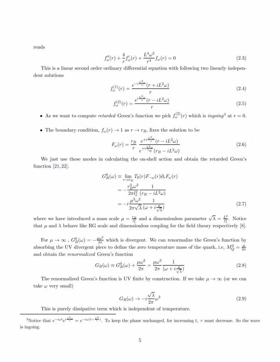
reads
f ′′ω(r) +
4
rf ′ω(r) +
L4ω2
r4fω(r) = 0 (2.3)
This is a linear second order ordinary differential equation with following two linearly indepen-
dent solutions
f (1)ω (r) =
e−iL2ωr (r + iL2ω)
r(2.4)
f (2)ω (r) =
eiL2ωr (r − iL2ω)
r(2.5)
• As we want to compute retarded Green’s function we pick f(2)ω (r) which is ingoing3 at r = 0.
• The boundary condition, fω(r) → 1 as r → rB, fixes the solution to be
Fω(r) =rBr
e+iL2ωr (r − iL2ω)
e+iL
2ωrB (rB − iL2ω)
(2.6)
We just use these modes in calculating the on-shell action and obtain the retarded Green’s
function [21,22].
G0R(ω) ≡ lim
r→rBT0(r)F−ω(r)∂rFω(r)
= −r2Bω2
2πl2s
1
(rB − iL2ω)
= −iµ2ω2
2π√λ
1
(ω + i µ√λ)
(2.7)
where we have introduced a mass scale µ = rBl2s
and a dimensionless parameter√λ = L2
l2s. Notice
that µ and λ behave like RG scale and dimensionless coupling for the field theory respectively [8].
For µ → ∞ , G0R(ω) = −µω2
2π which is divergent. We can renormalize the Green’s function by
absorbing the UV divergent piece to define the zero temperature mass of the quark, i.e, M0Q = µ
2π
and obtain the renormalized Green’s function
GR(ω) ≡ G0R(ω) +
µω2
2π=
µω3
2π
1
(ω + i µ√λ)
(2.8)
The renormalized Green’s function is UV finite by construction. If we take µ → ∞ (or we can
take ω very small)
GR(ω) → −i
√λ
2πω3 (2.9)
This is purely dissipative term which is independent of temperature.
3Notice that e−iωteiL2ω
r = e−iω(t−L2
r). To keep the phase unchanged, for increasing t, r must decrease. So the wave
is ingoing.
5
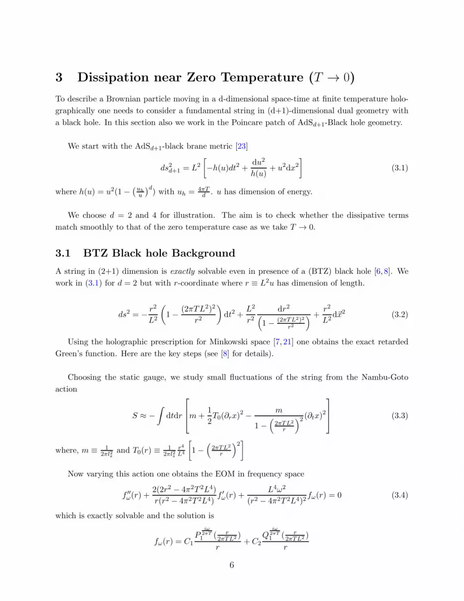
3 Dissipation near Zero Temperature (T → 0)
To describe a Brownian particle moving in a d-dimensional space-time at finite temperature holo-
graphically one needs to consider a fundamental string in (d+1)-dimensional dual geometry with
a black hole. In this section also we work in the Poincare patch of AdSd+1-Black hole geometry.
We start with the AdSd+1-black brane metric [23]
ds2d+1 = L2
[
−h(u)dt2 +du2
h(u)+ u2dx2
]
(3.1)
where h(u) = u2(1−(uh
u
)d) with uh = 4πT
d . u has dimension of energy.
We choose d = 2 and 4 for illustration. The aim is to check whether the dissipative terms
match smoothly to that of the zero temperature case as we take T → 0.
3.1 BTZ Black hole Background
A string in (2+1) dimension is exactly solvable even in presence of a (BTZ) black hole [6, 8]. We
work in (3.1) for d = 2 but with r-coordinate where r ≡ L2u has dimension of length.
ds2 = − r2
L2
(
1− (2πTL2)2
r2
)
dt2 +L2
r2dr2
(
1− (2πTL2)2
r2
) +r2
L2d~x2 (3.2)
Using the holographic prescription for Minkowski space [7, 21] one obtains the exact retarded
Green’s function. Here are the key steps (see [8] for details).
Choosing the static gauge, we study small fluctuations of the string from the Nambu-Goto
action
S ≈ −∫
dtdr
m+
1
2T0(∂rx)
2 − m
1−(2πTL2
r
)2 (∂tx)2
(3.3)
where, m ≡ 12πl2s
and T0(r) ≡ 12πl2s
r4
L4
[
1−(2πTL2
r
)2]
Now varying this action one obtains the EOM in frequency space
f ′′ω(r) +
2(2r2 − 4π2T 2L4)
r(r2 − 4π2T 2L4)f ′ω(r) +
L4ω2
(r2 − 4π2T 2L4)2fω(r) = 0 (3.4)
which is exactly solvable and the solution is
fω(r) = C1P
iω2πT
1 ( r2πTL2 )
r+ C2
Qiω
2πT
1 ( r2πTL2 )
r
6
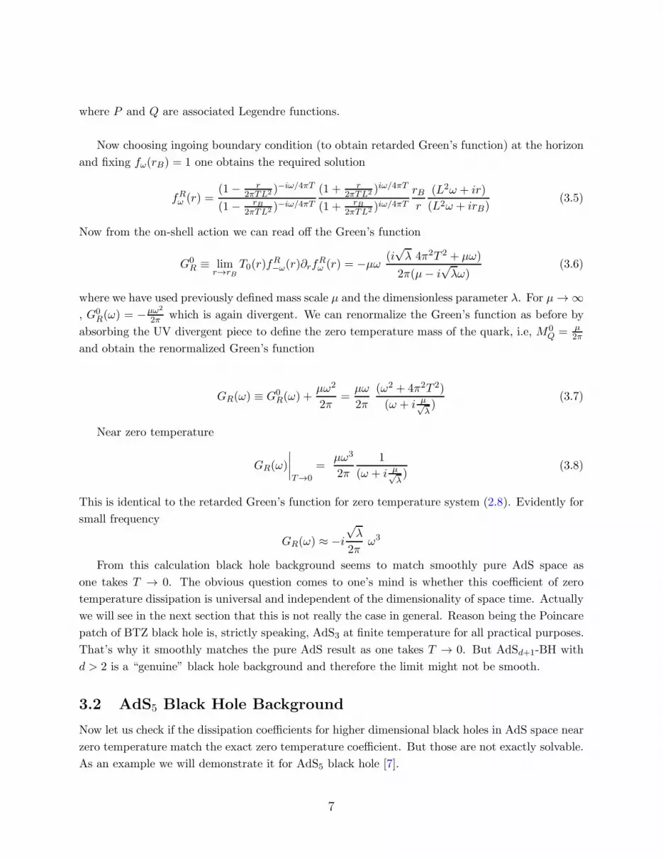
where P and Q are associated Legendre functions.
Now choosing ingoing boundary condition (to obtain retarded Green’s function) at the horizon
and fixing fω(rB) = 1 one obtains the required solution
fRω (r) =
(1− r2πTL2 )
−iω/4πT
(1− rB2πTL2 )−iω/4πT
(1 + r2πTL2 )
iω/4πT
(1 + rB2πTL2 )iω/4πT
rBr
(L2ω + ir)
(L2ω + irB)(3.5)
Now from the on-shell action we can read off the Green’s function
G0R ≡ lim
r→rBT0(r)f
R−ω(r)∂rf
Rω (r) = −µω
(i√λ 4π2T 2 + µω)
2π(µ− i√λω)
(3.6)
where we have used previously defined mass scale µ and the dimensionless parameter λ. For µ → ∞, G0
R(ω) = −µω2
2π which is again divergent. We can renormalize the Green’s function as before by
absorbing the UV divergent piece to define the zero temperature mass of the quark, i.e, M0Q = µ
2π
and obtain the renormalized Green’s function
GR(ω) ≡ G0R(ω) +
µω2
2π=
µω
2π
(ω2 + 4π2T 2)
(ω + i µ√λ)
(3.7)
Near zero temperature
GR(ω)
∣∣∣∣T→0
=µω3
2π
1
(ω + i µ√λ)
(3.8)
This is identical to the retarded Green’s function for zero temperature system (2.8). Evidently for
small frequency
GR(ω) ≈ −i
√λ
2πω3
From this calculation black hole background seems to match smoothly pure AdS space as
one takes T → 0. The obvious question comes to one’s mind is whether this coefficient of zero
temperature dissipation is universal and independent of the dimensionality of space time. Actually
we will see in the next section that this is not really the case in general. Reason being the Poincare
patch of BTZ black hole is, strictly speaking, AdS3 at finite temperature for all practical purposes.
That’s why it smoothly matches the pure AdS result as one takes T → 0. But AdSd+1-BH with
d > 2 is a “genuine” black hole background and therefore the limit might not be smooth.
3.2 AdS5 Black Hole Background
Now let us check if the dissipation coefficients for higher dimensional black holes in AdS space near
zero temperature match the exact zero temperature coefficient. But those are not exactly solvable.
As an example we will demonstrate it for AdS5 black hole [7].
7
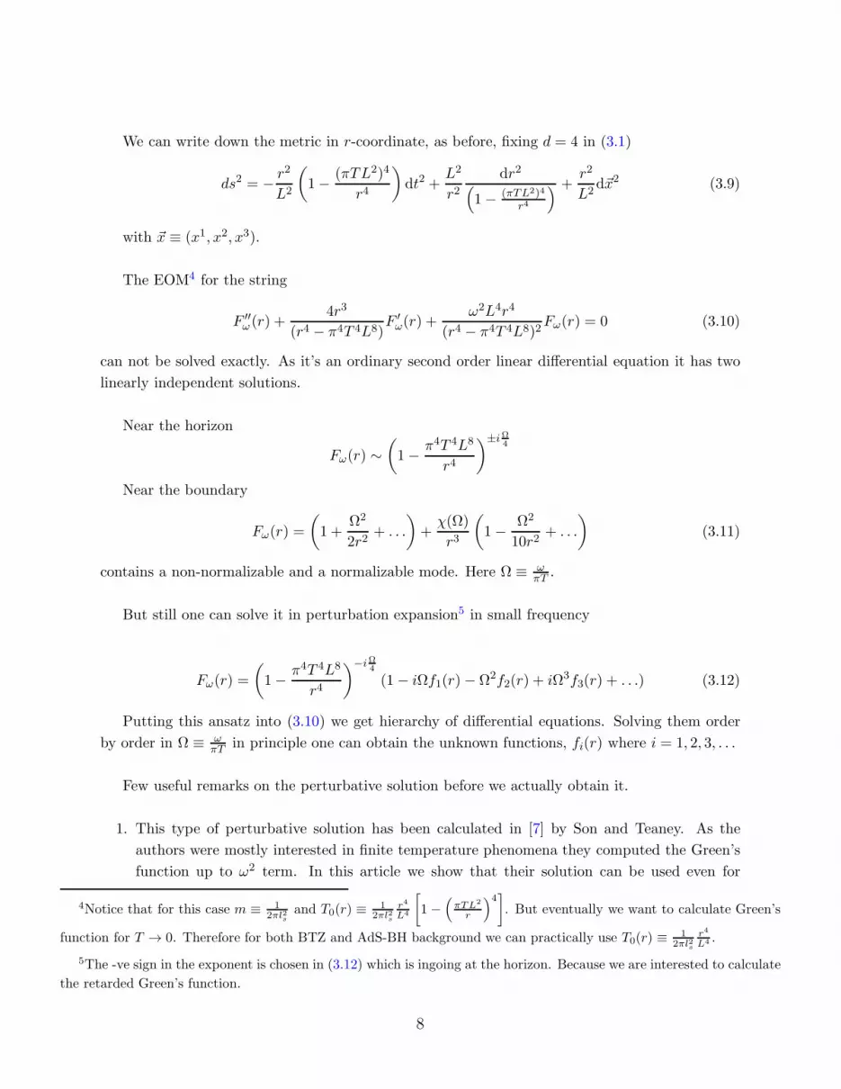
We can write down the metric in r-coordinate, as before, fixing d = 4 in (3.1)
ds2 = − r2
L2
(
1− (πTL2)4
r4
)
dt2 +L2
r2dr2
(
1− (πTL2)4
r4
) +r2
L2d~x2 (3.9)
with ~x ≡ (x1, x2, x3).
The EOM4 for the string
F ′′ω (r) +
4r3
(r4 − π4T 4L8)F ′ω(r) +
ω2L4r4
(r4 − π4T 4L8)2Fω(r) = 0 (3.10)
can not be solved exactly. As it’s an ordinary second order linear differential equation it has two
linearly independent solutions.
Near the horizon
Fω(r) ∼(
1− π4T 4L8
r4
)±iΩ4
Near the boundary
Fω(r) =
(
1 +Ω2
2r2+ . . .
)
+χ(Ω)
r3
(
1− Ω2
10r2+ . . .
)
(3.11)
contains a non-normalizable and a normalizable mode. Here Ω ≡ ωπT .
But still one can solve it in perturbation expansion5 in small frequency
Fω(r) =
(
1− π4T 4L8
r4
)−iΩ4
(1− iΩf1(r)− Ω2f2(r) + iΩ3f3(r) + . . .) (3.12)
Putting this ansatz into (3.10) we get hierarchy of differential equations. Solving them order
by order in Ω ≡ ωπT in principle one can obtain the unknown functions, fi(r) where i = 1, 2, 3, . . .
Few useful remarks on the perturbative solution before we actually obtain it.
1. This type of perturbative solution has been calculated in [7] by Son and Teaney. As the
authors were mostly interested in finite temperature phenomena they computed the Green’s
function up to ω2 term. In this article we show that their solution can be used even for
4Notice that for this case m ≡ 12πl2
s
and T0(r) ≡ 12πl2
s
r4
L4
[
1−(
πTL2
r
)4]
. But eventually we want to calculate Green’s
function for T → 0. Therefore for both BTZ and AdS-BH background we can practically use T0(r) ≡ 12πl2
s
r4
L4 .
5The -ve sign in the exponent is chosen in (3.12) which is ingoing at the horizon. Because we are interested to calculate
the retarded Green’s function.
8
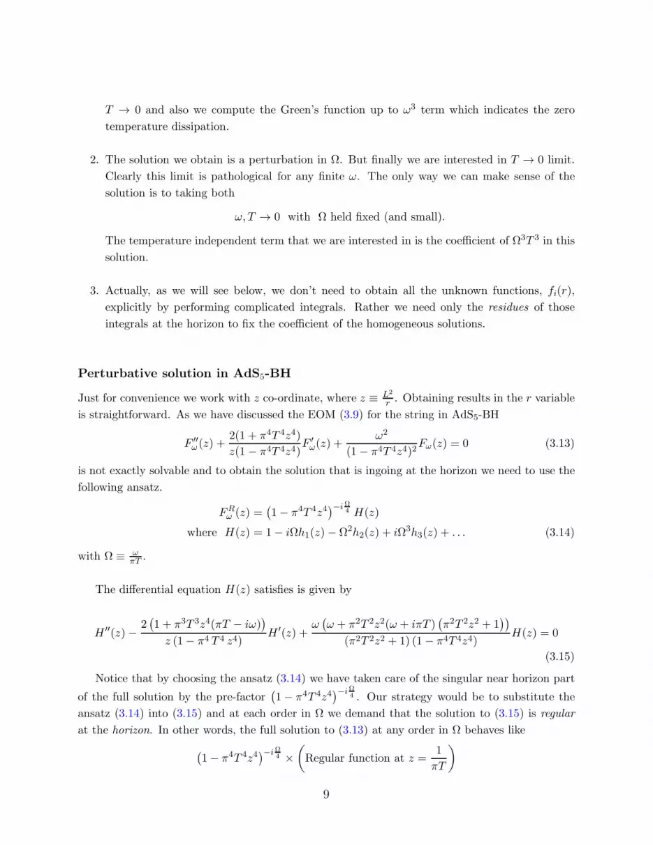
T → 0 and also we compute the Green’s function up to ω3 term which indicates the zero
temperature dissipation.
2. The solution we obtain is a perturbation in Ω. But finally we are interested in T → 0 limit.
Clearly this limit is pathological for any finite ω. The only way we can make sense of the
solution is to taking both
ω, T → 0 with Ω held fixed (and small).
The temperature independent term that we are interested in is the coefficient of Ω3T 3 in this
solution.
3. Actually, as we will see below, we don’t need to obtain all the unknown functions, fi(r),
explicitly by performing complicated integrals. Rather we need only the residues of those
integrals at the horizon to fix the coefficient of the homogeneous solutions.
Perturbative solution in AdS5-BH
Just for convenience we work with z co-ordinate, where z ≡ L2
r . Obtaining results in the r variable
is straightforward. As we have discussed the EOM (3.9) for the string in AdS5-BH
F ′′ω (z) +
2(1 + π4T 4z4)
z(1 − π4T 4z4)F ′ω(z) +
ω2
(1− π4T 4z4)2Fω(z) = 0 (3.13)
is not exactly solvable and to obtain the solution that is ingoing at the horizon we need to use the
following ansatz.
FRω (z) =
(1− π4T 4z4
)−iΩ4 H(z)
where H(z) = 1− iΩh1(z)− Ω2h2(z) + iΩ3h3(z) + . . . (3.14)
with Ω ≡ ωπT .
The differential equation H(z) satisfies is given by
H ′′(z)− 2(1 + π3T 3z4(πT − iω)
)
z (1− π4 T 4 z4)H ′(z) +
ω(ω + π2T 2z2(ω + iπT )
(π2T 2z2 + 1
))
(π2T 2z2 + 1) (1− π4T 4z4)H(z) = 0
(3.15)
Notice that by choosing the ansatz (3.14) we have taken care of the singular near horizon part
of the full solution by the pre-factor(1− π4T 4z4
)−iΩ4 . Our strategy would be to substitute the
ansatz (3.14) into (3.15) and at each order in Ω we demand that the solution to (3.15) is regular
at the horizon. In other words, the full solution to (3.13) at any order in Ω behaves like
(1− π4T 4z4
)−iΩ4 ×
(
Regular function at z =1
πT
)
9
.
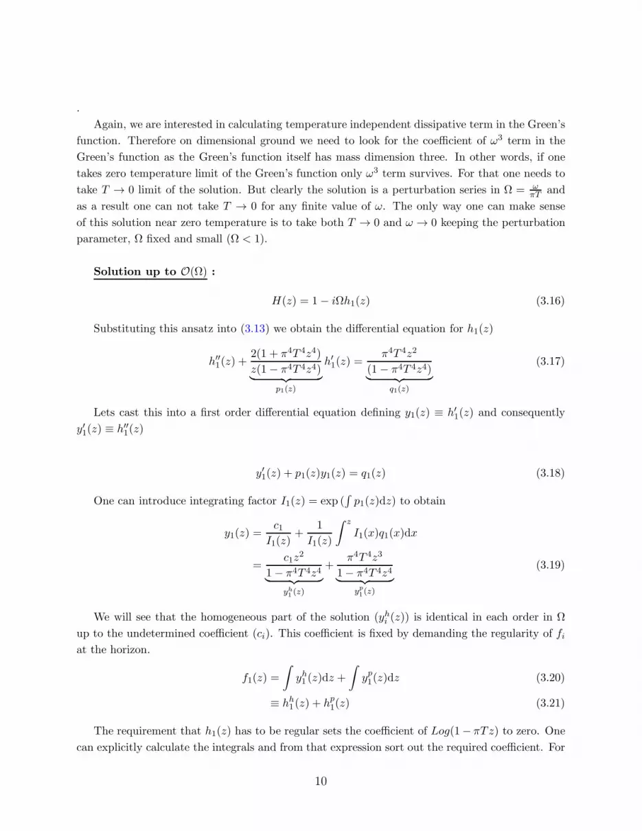
Again, we are interested in calculating temperature independent dissipative term in the Green’s
function. Therefore on dimensional ground we need to look for the coefficient of ω3 term in the
Green’s function as the Green’s function itself has mass dimension three. In other words, if one
takes zero temperature limit of the Green’s function only ω3 term survives. For that one needs to
take T → 0 limit of the solution. But clearly the solution is a perturbation series in Ω = ωπT and
as a result one can not take T → 0 for any finite value of ω. The only way one can make sense
of this solution near zero temperature is to take both T → 0 and ω → 0 keeping the perturbation
parameter, Ω fixed and small (Ω < 1).
Solution up to O(Ω) :
H(z) = 1− iΩh1(z) (3.16)
Substituting this ansatz into (3.13) we obtain the differential equation for h1(z)
h′′1(z) +2(1 + π4T 4z4)
z(1− π4T 4z4)︸ ︷︷ ︸
p1(z)
h′1(z) =π4T 4z2
(1− π4T 4z4)︸ ︷︷ ︸
q1(z)
(3.17)
Lets cast this into a first order differential equation defining y1(z) ≡ h′1(z) and consequently
y′1(z) ≡ h′′1(z)
y′1(z) + p1(z)y1(z) = q1(z) (3.18)
One can introduce integrating factor I1(z) = exp (∫p1(z)dz) to obtain
y1(z) =c1
I1(z)+
1
I1(z)
∫ z
I1(x)q1(x)dx
=c1z
2
1− π4T 4z4︸ ︷︷ ︸
yh1(z)
+π4T 4z3
1− π4T 4z4︸ ︷︷ ︸
yp1(z)
(3.19)
We will see that the homogeneous part of the solution (yhi (z)) is identical in each order in Ω
up to the undetermined coefficient (ci). This coefficient is fixed by demanding the regularity of fi
at the horizon.
f1(z) =
∫
yh1 (z)dz +
∫
yp1(z)dz (3.20)
≡ hh1 (z) + hp1(z) (3.21)
The requirement that h1(z) has to be regular sets the coefficient of Log(1− πTz) to zero. One
can explicitly calculate the integrals and from that expression sort out the required coefficient. For
10
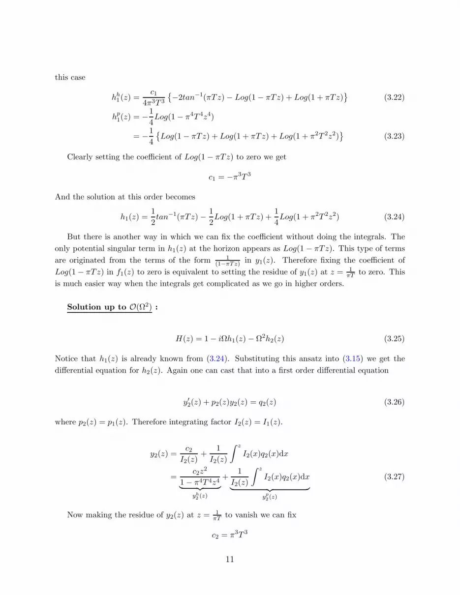
this case
hh1(z) =c1
4π3T 3
−2tan−1(πTz)− Log(1− πTz) + Log(1 + πTz)
(3.22)
hp1(z) = −1
4Log(1− π4T 4z4)
= −1
4
Log(1− πTz) + Log(1 + πTz) + Log(1 + π2T 2z2)
(3.23)
Clearly setting the coefficient of Log(1− πTz) to zero we get
c1 = −π3T 3
And the solution at this order becomes
h1(z) =1
2tan−1(πTz)− 1
2Log(1 + πTz) +
1
4Log(1 + π2T 2z2) (3.24)
But there is another way in which we can fix the coefficient without doing the integrals. The
only potential singular term in h1(z) at the horizon appears as Log(1 − πTz). This type of terms
are originated from the terms of the form 1(1−πTz) in y1(z). Therefore fixing the coefficient of
Log(1− πTz) in f1(z) to zero is equivalent to setting the residue of y1(z) at z = 1πT to zero. This
is much easier way when the integrals get complicated as we go in higher orders.
Solution up to O(Ω2) :
H(z) = 1− iΩh1(z)− Ω2h2(z) (3.25)
Notice that h1(z) is already known from (3.24). Substituting this ansatz into (3.15) we get the
differential equation for h2(z). Again one can cast that into a first order differential equation
y′2(z) + p2(z)y2(z) = q2(z) (3.26)
where p2(z) = p1(z). Therefore integrating factor I2(z) = I1(z).
y2(z) =c2
I2(z)+
1
I2(z)
∫ z
I2(x)q2(x)dx
=c2z
2
1− π4T 4z4︸ ︷︷ ︸
yh2(z)
+1
I2(z)
∫ z
I2(x)q2(x)dx
︸ ︷︷ ︸
yp2(z)
(3.27)
Now making the residue of y2(z) at z = 1πT to vanish we can fix
c2 = π3T 3
11
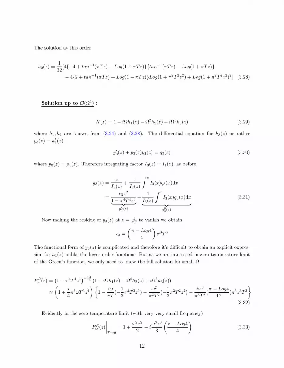
The solution at this order
h2(z) =1
32[4−4 + tan−1(πTz)− Log(1 + πTz)tan−1(πTz)− Log(1 + πTz)
− 42 + tan−1(πTz)− Log(1 + πTz)Log(1 + π2T 2z2) + Log(1 + π2T 2z2)2] (3.28)
Solution up to O(Ω3) :
H(z) = 1− iΩh1(z)− Ω2h2(z) + iΩ3h3(z) (3.29)
where h1, h2 are known from (3.24) and (3.28). The differential equation for h3(z) or rather
y3(z) ≡ h′3(z)
y′3(z) + p3(z)y2(z) = q3(z) (3.30)
where p3(z) = p1(z). Therefore integrating factor I3(z) = I1(z), as before.
y3(z) =c3
I3(z)+
1
I3(z)
∫ z
I3(x)q3(x)dx
=c3z
2
1− π4T 4z4︸ ︷︷ ︸
yh3(z)
+1
I3(z)
∫ z
I3(x)q3(x)dx
︸ ︷︷ ︸
yp3(z)
(3.31)
Now making the residue of y3(z) at z = 1πT to vanish we obtain
c3 =
(π − Log4
4
)
π3T 3
The functional form of y3(z) is complicated and therefore it’s difficult to obtain an explicit expres-
sion for h3(z) unlike the lower order functions. But as we are interested in zero temperature limit
of the Green’s function, we only need to know the full solution for small Ω
FRω (z) =
(1− π4T 4z4
)−iΩ4 (1− iΩh1(z)− Ω2h2(z) + iΩ3h3(z))
≈(
1 +i
4π3ωT 3z4
)
1− iω
πT(−1
3π3T 3z3)− ω2
π2T 2(−1
3π2T 2z2)− iω3
π3T 3(π − Log4
12)π3z3T 3
(3.32)
Evidently in the zero temperature limit (with very very small frequency)
FRω (z)
∣∣∣∣T→0
= 1 +ω2z2
2+ i
ω3z3
3
(π − Log4
4
)
(3.33)
12

In r co-ordinate
FRω (r)
∣∣∣∣T→0
= 1 +ω2L4
2r2+ i
ω3L6
3r3
(π − Log4
4
)
(3.34)
The retarded Green’s function at T = 0 can be calculated using the solution (3.34)
G0R ≡ lim
r→rBT0(r)F
R−ω(r)∂rF
Rω (r)
= limr→rB
1
2πl2s
r4
L4
(
−ω2L4
r3− i
ω3L6
4r4(π − Log4)
)
= −µω2
2π− i
√λ
2π
(π − Log4
4
)
ω3 (3.35)
Therefore the renormalized Green’s function
GR(ω) ≡ G0R +
µω2
2π= −i
√λ
2π
(π − Log4
4
)
ω3 (3.36)
It is evident that this zero temperature dissipation term is not same as that of pure AdS case
and actually off by a factor of π−Log44 .
4 Discussions
Whenever a charged particle accelerates or decelerates it radiates energy which is known as brehm-
strahlung effect. In this paper we talk about dissipation at and near zero temperature. Naturally
this zero temperature dissipation finds its origin in this brehmstrahlung phenomenon. One can
notice that this dissipative force term (Fdiss) goes as a cubic power in frequency
Fdiss(ω) ∼ −i√λ ω3x(ω)
In real space this each iω gives a time derivative and therefore the above force law reduces to
Fdiss(t) ∼√λ...x (t) =
√λ a
a here quantifies the rate of change in acceleration and is often called jerk or jolt. This formula
is very similar to that of “Abraham-Lorentz force” [32] in classical electrodynamics for a charged
particle with charge q
Frad(t) =2
3q2 a
This is the force that an accelerating charged particle feels in the recoil from the emission of ra-
diation. Only the effective coupling is different for the holographic case. This “coupling”(√λ) is
essentially the brehmstrahlung function B(λ,N). The corrections in λ and N can also be computed
for particular known theories (see [27–30]).
13
The main aim in this paper is to understand how this brehmstrahlung function behaves near
zero temperature. We work in Poincare patch of AdS-black hole on the gravity side. We notice
that for higher dimensional cases (we performed calculations in AdS5-BH) value of this function6
near T → 0 doesn’t match that of at T = 0. Actually this result is not unexpected as there is a
Hawking-Page phase transition at zero temperature in Poincare patch of black holes in AdS.
One the other hand we see that for a particle in 1+1 dimensional field theory the bremsstrahlung
function matches smoothly at T = 0. The possible reason behind this phenomenon is hidden in
the corresponding dual geometries namely AdS3 (for T = 0) and BTZ (at T 6= 0). A BTZ black
hole is just an orbifold of AdS3 and therefore locally AdS3. One can only distinguish the former
from the latter by studying global properties. BTZ in Poincare patch is no different than AdS3
at finite temperature (also called thermal AdS3) unlike the higher dimensional black holes in AdS
which are “genuine” black hole backgrounds.
5 Conclusions
We summarize the main points here:
• We have studied Brownian motion in various space time dimensions with the help of holo-
graphic Green’s function computation. In each case we obtain dissipation at zero temperature
due to radiation from accelerated charged Brownian particle.
• As long as we are considering Brownian motion in zero temperature, that is the string in
the dual gravity theory moves in a pure AdS spacetime, the coefficients of dissipation for
arbitrary space time dimensions are identical. The value of the coefficient is√λ
2π and can
be identified with B(λ,N) (2πB(λ,N) =√λ
2π ) identified in [26] as occurring in many other
physical quantities (such as the cusp anomalous dimension introduced by Polyakov [31]).
• Even the coefficients match for string in AdS3 and in BTZ as we take T → 0. This is because
BTZ in Poincare patch is nothing more than a thermal AdS3.
• For higher dimensions the coefficients at T = 0 and T → 0 don’t match. Thus one should
be careful when using pure AdS for calculating near zero temperature quantities. We have
shown this phenomenon via explicit computation by studying a string dynamics in AdS5-BH
background. The corresponding coefficient comes out to be√λ
2ππ−Log4
4 . This phenomenon
might have its origin in the Hawking-Page transition at T = 0 in Poincare patch.
6Of course we are working in leading order in large-N and large-λ. To compute corrections one needs to work with
some known supersymmetric UV theories (e.g, ABJM, N = 4 SYM)
14
A Perturbative solution for string in BTZ
We already mentioned that EOM for a string in BTZ can be solved exactly and hence one can
compute exact retarded Green’s function for the Brownian particle. Actually we have done the
same in 3.2. There we have seen that the zero temperature dissipation coefficient is√λ
2π . On the
other hand, the EOM of string in AdS5-BH is not exactly solvable and therefore we adopted a
perturbative technique to compute the above mentioned coefficient. In 3.2 we got a different value
for that coefficient. In this section we apply the same perturbative method for a string in BTZ
and show that the same result for zero temperature dissipation is reproduced. This is just to show
that the perturbative approach and the associated limits indeed work.
Our aim is to perturbatively solve (3.4) which in z-coordinate looks
f ′′ω(z) +
2
z(1 − 4π2T 2z2)f ′ω(z) +
ω2
(1− 4π2T 2z2)2fω(z) = 0 (A.1)
using the following ansatz
fRω (z) =
(1− 4π2T 2z2
)−iΩ2 (1− iΩh1(z)− Ω2h2(z) + iΩ3h3(z) + . . .) (A.2)
where in this section Ω ≡ ω2πT (notice the extra factor of two).
Again we will be working in the regime where
ω, T → 0 with Ω held fixed (and small).
Next step is to solve for the unknown functions, h1(x), h2(x), h3(x) etc. recursively. We repeat
the same procedure as in (3.2).
Solution up to O(Ω) :
fω(z) =(1− 4π2T 2z2
)−iΩ2 (1− iΩh1(z)) (A.3)
Substituting this ansatz into (A.1) we obtain the differential equation for h1(z)
h′′1(z) −2
z(1− 4π2T 2z2)︸ ︷︷ ︸
p1(z)
h′1(z) = − 4π2T 2
(1− 4π2T 2z2)︸ ︷︷ ︸
q1(z)
(A.4)
Lets cast this into a first order differential equation defining y1(z) ≡ f ′1(z) and consequently
y′1(z) ≡ f ′′1 (z)
y′1(z) + p1(z)y1(z) = q1(z) (A.5)
15
Introducing the integrating factor I1(z) = exp (∫p1(z)dz)
y1(z) =c1
I1(z)+
1
I1(z)
∫ z
I1(x)q1(x)dx
=c1z
2
1− 4π2T 2z2︸ ︷︷ ︸
yh1(z)
+4π2T 2z
1− 4π2T 2z2︸ ︷︷ ︸
yp1(z)
(A.6)
The homogeneous part of the solution (yhi (z)) will again be identical in each order in Ω up to
the undetermined coefficient (ci). This coefficient is fixed by demanding the regularity of hi at the
horizon.
h1(z) =
∫
yh1 (z)dz +
∫
yp1(z)dz (A.7)
≡ hh1 (z) + hp1(z) (A.8)
Demanding regularity for h1(z) fixes the coefficient of Log(1−2πTz) to zero. One can explicitly
calculate the integrals and from that expression sort out the required coefficient. For this case
hh1 (z) = c1
[
− z
4π2T 2+
1
16π3T 3Log(1 + 2πTz)− Log(1 − 2πTz)
]
(A.9)
hp1(z) = −1
2Log(1 − 4π2T 2z2)
= −1
2Log(1 + 2πTz) + Log(1 − 2πTz) (A.10)
Clearly setting the coefficient of Log(1− 2πTz) to zero we get
c1 = −8π3T 3
And the solution at this order becomes
h1(z) =1
2[4πTz − 2Log(1 + 2πTz)] (A.11)
As has been argued before we can equivalently set the residue of y1(z) at z = 12πT to zero to
fix the value of c1.
Solution up to O(Ω2) :
fω(z) =(1− 4π2T 2z2
)−iΩ2 (1− iΩh1(z)− Ω2h2(z)) (A.12)
h1(z) is already known from (A.11). The differential equation for h2(z) reduces to
y′2(z) + p2(z)y2(z) = q2(z) (A.13)
16

where p2(z) = p1(z) and integrating factor I2(z) = I1(z).
y2(z) =c2
I2(z)+
1
I2(z)
∫ z
I2(x)q2(x)dx
=c2z
2
1− 4π2T 2z2︸ ︷︷ ︸
yh2(z)
+1
I2(z)
∫ z
I2(x)q2(x)dx
︸ ︷︷ ︸
yp2(z)
(A.14)
Now making the residue of y2(z) at z = 12πT to vanish we can fix
c2 = 8π3T 3
The solution at this order
h2(z) =1
2
[−4πTz + Log(1 + 2πTz)2
](A.15)
Solution up to O(Ω3) :
fω(z) =(1− 4π2T 2z2
)−iΩ2 (1− iΩh1(z)− Ω2h2(z) + iΩ3h3(z)) (A.16)
where h1, h2 are known from (A.11) and (A.19). The differential equation for h3(z) or rather
y3(z) ≡ h′3(z)
y′3(z) + p3(z)y2(z) = q3(z) (A.17)
where p3(z) = p1(z) and thus integrating factor I3(z) = I1(z), as before.
y3(z) =c3
I3(z)+
1
I3(z)
∫ z
I3(x)q3(x)dx
=c3z
2
1− 4π2T 2z2︸ ︷︷ ︸
yh3(z)
+1
I3(z)
∫ z
I3(x)q3(x)dx
︸ ︷︷ ︸
yp3(z)
(A.18)
Now fixing residue of y3(z) at z = 12πT to vanish we obtain
c3 = 0
The functional form of h3(z) is simple unlike the higher dimensional case.
h3(z) = πTzLog(1 + 2πTz)2 − 1
6Log(1 + 2πTz)3 (A.19)
17
Therefore in this perturbative expansion the full solution becomes
fRω (z) =
(1− 4π2T 2z2
)−iΩ2 (1−iΩ(
1
2(4πTz − 2Log(1 + 2πTz))) − Ω2(
1
2(−4πTz + Log(1 + 2πTz)2))
+iΩ3(πTzLog(1 + 2πTz)2 − 1
6Log(1 + 2πTz)3)) (A.20)
Evidently in the zero temperature limit (with very small frequency)
fRω (z)
∣∣∣∣T→0
= 1 +ω2z2
2+ i
ω3z3
3(A.21)
In r co-ordinate
fRω (r)
∣∣∣∣T→0
= 1 +ω2L4
2r2+ i
ω3L6
3r3(A.22)
The retarded Green’s function at T = 0 can be calculated using this solution
G0R ≡ lim
r→rBT0(r)f
R−ω(r)∂rf
Rω (r)
= limr→rB
1
2πl2s
r4
L4
(
−ω2L4
r3− i
ω3L6
r4
)
= −µω2
2π− i
√λ
2πω3 (A.23)
Thus the renormalized Green’s function
GR(ω) ≡ G0R +
µω2
2π= −i
√λ
2πω3 (A.24)
This matches identically with the leading term in small frequency expansion of (3.8).
References
[1] J. M. Maldacena, “The large N limit of superconformal field theories and supergravity”, Adv.
Theor. Math. Phys. 2 (1998) 231. [hep-th/9711200]
[2] S. S. Gubser, I. R. Klebanov and A. M. Polyakov, “Gauge theory correlators from non-critical
string theory”, Phys. Lett. B 428 (1998) 105. [hep-th/9802109]
[3] E. Witten, “Anti-de Sitter space and holography”, Adv. Theor. Math. Phys. 2 (1998) 253.
[hep-th/9802150]
18
[4] E. Witten, “Anti-de Sitter space, thermal phase transition, and confinement in gauge theories”,
Adv. Theor. Math. Phys 2 (1998) 505. [hep-th/9803131]
[5] G. Policastro, D. T. Son and A. O. Starinets, “The Shear viscosity of strongly coupled N=4
supersymmetric Yang-Mills plasma,” Phys. Rev. Lett. 87 (2001) 081601 [hep- th/0104066]
[6] J. de Boer, V. E. Hubeny, M. Rangamani, M Shigemori, “Brownian motion in AdS/CFT”,
JHEP 0907, (2009) 094 [arXiv:0812.5112[hep-th]]
[7] D. T. Son and D. Teaney, “Thermal Noise and Stochastic Strings in AdS/CFT”, JHEP 0907
, (2009) 021. [arXiv:0901.2338[hep-th]]
[8] P. Banerjee and B. Sathiapalan “Holographic Brownian Motion in 1+1 Dimensions,” Nucl.
Phys. B 884 (2014) 74-105 [arXiv: 1308.3352 [hep-th]].
[9] A.Mikhailov, “Nonlinear waves in AdS/CFT correspondence”, [hep-th/0305196]
[10] B. -W. Xiao, “On the exact solution of the accelerating string in AdS(5) space,” Phys. Lett.
B 665 (2008) 173 [arXiv:0804.1343 [hep-th]].
[11] E. Caceres, M. Chernicoff, A. Guijosa, J. F. Pedraza, “Quantum Fluctuations and the
Unruh Effect in Strongly-Coupled Conformal Field Theories”, JHEP 1006 , (2010) 078.
[arXiv:1003.5332[hep-th]]
[12] Y. Hatta, E. Iancu, A.H. Mueller, D.N. Triantafyllopoulos, “Radiation by a heavy quark in
N=4 SYM at strong coupling”, Nucl.Phys. B 850 (2011) 31-52. [arXiv:1102.0232 [hep-th]]
[13] M. Chernicoff, A. Guijosa and J. F. Pedraza,“The Gluonic Field of a Heavy Quark in Con-
formal Field Theories at Strong Coupling”, JHEP 1110 (2011) 041. [arXiv:1106.4059[hep-th]]
[14] M. Chernicoff, J. A. Garcia, A. Guijosa and J. F. Pedraza, “Holographic Lessons for Quark
Dynamics”, J. Phys. G G 39, 054002 (2012) [arXiv:1111.0872 [hep-th]].
[15] M. Chernicoff, J. A. Garcia and A. Guijosa, “Generalized Lorentz-Dirac Equation for a
Strongly-Coupled Gauge Theory”, Phys.Rev.Lett. 102 (2009) 241601. [arXiv:0903.2047[hep-
th]]
[16] M. Chernicoff, J. A. Garcia and A. Guijosa, “A Tail of a Quark in N = 4 SYM”, JHEP 0909
(2009) 080. [arXiv:0906.1592[hep-th]]
19
[17] M. Chernicoff and A. Guijosa, “Acceleration, Energy Loss and Screening in Strongly-Coupled
Gauge Theories”, JHEP 0806 (2008) 005. [arXiv:0803.3070[hep-th]]
[18] T. Fulton and F. Rohrlich, “Classical radiation from a uniformly accelerated charge”, Annals
Phys.9, 499 (1960).
[19] D. G. Boulware, “Radiation From a Uniformly Accelerated Charge”, Annals Phys. 124, 169
(1980)
[20] D. Correa, J. Henn, J. Maldacena and A. Sever, “An exact formula for the radiation of
a moving quark in N = 4 super Yang Mills,” JHEP 1206, 048 (2012) [arXiv:1202.4455 [hep-th]]
[21] D. T. Son and A. O. Starinets, “Minkowski-space correlators in AdS/CFT correspondence:
recipe and applications” , JHEP 0209, (2002) 042. [hep-th/0205051]
[22] C. P. Herzog and D. T. Son, “Schwinger-Keldysh propagators from AdS/CFT correspon-
dence”, JHEP 0303, (2003) 046 [hep-th/0212072]
[23] C. P. Herzog, A. Karch, P. Kovtun, C. Kozcaz and L. G. Yaffe, “Energy loss of a heavy
quark moving through N = 4 supersymmetric Yang-Mills plasma”, JHEP 0607, (2006) 013.
[hep-th/0605158]
[24] W. Fischler, J. F. Pedraza and W. T. Garcia, “Holographic Brownian Motion in Magnetic
Environments”, JHEP 1212, (2012) 002. [arXiv:1209.1044[hep-th]]
[25] S. W. Hawking and D. N. Page, “Thermodynamics of Black Holes in Anti-de Sitter Space”,
Commun. Math. Phys. 87, 577-588 (1983)
[26] A. Lewkowycz and J. Maldacena, “Exact results for the entanglement entropy and the energy
radiated by a quark”, [arxiv: 1312.5682 [hep-th]]
[27] B. Fiol and B. Garolera, “Energy Loss of an Infinitely Massive Half-Bogomol’nyi-Prasad-
Sommerfeld Particle by Radiation to All Orders in 1/N” Phys.Rev.Lett. 107 (2011) 151601
[arXiv:1106.5418 [hep-th]]
[28] B. Fiol, B. Garolera and A. Lewkowycz, “Exact results for static and radiative fields of a
quark in N=4 super Yang-Mills,” JHEP 1205, 093 (2012) [arXiv:1202.5292 [hep-th]]
20
[29] Exact momentum fluctuations of an accelerated quark in N = 4 super Yang-Mills B. Fiol ,
B. Garolera and G. Torrents JHEP 1306, 011 (2013) [arXiv:1302.6991 [hep-th]]
[30] B. Fiol, E. Gerchkovitz and Z. Komargodski, “The Exact Bremsstrahlung Function in N = 2
Superconformal Field Theories” [arXiv : 1510.01332[hep-th]]
[31] A. M. Polyakov “Gauge fields as rings of glue,” Nucl. Phys. B 164 (1980) 171-188
[32] D. J. Griffiths “Introduction to Electrodynamics” 3rd Edition (2009)
***
21