digital holography techniques for optical microscopy
TRANSCRIPT
Florian Soulard
Master of Micro and Nanotechnologies for Integrated Systems
Research Master in Micro and Nano Electronics
2007 to 2009
Digital holography techniques
for optical microscopy
Department of Physics – Rome III University
Supervisor: Pr. Massimo Santarsiero
Dipartimento di Fisica "E. Amaldi"
via della Vasca Navale, 84
00146 ROMA - ITALIA
Acknowledgements
I would like to express my gratitude to my supervisor in Rome, Prof. Massimo
Santarsiero, for his kindness and his patience all along the internship. His advices and
suggestions were very useful when I encountered some problems with the techniques
presented in this report.
I acknowledge Prof. Franco Gori for the very good book he wrote, “Elementi di Ottica”.
This book was very useful to understand the principles of holography, and for
explaining the propagation method that was numerically implemented for the
holographic reconstruction. Additionally, I learnt the Italian vocabulary for optics while
reading it…
This internship would not have been possible without the agreement of Ms. Panagiota
Morfouli, responsible of the Master MNIS in Grenoble, and Mr. Jean-Pierre Petit, co-
director of PHELMA, who allowed me to work on a topic in which I have a strong
interest.
I would also like to thank my supervisor in Grenoble, Ms. Liliana Buda-Prejbeanu, for
the information provided, especially at the end of the internship. A special thanks for
the administrative staff in Grenoble too, in particular Ms. Eliane Zammit, for the helpful
documents I was sent to help me during my stay abroad.
I am grateful to the Rhones-Alpes region, for the financial support I was granted
through the “Explo’RA” scholarship.
Finally, I want to thank my family and my friends for their support.
Contents
Introduction ................................................................................................................. 1
1. Light properties, and principles of holography ...................................... 3
1.1. Nature of light ........................................................................................................ 3
1.2. Plane waves and spherical waves ......................................................................... 4
1.3. Photography versus holography........................................................................... 5
1.4. The optical set-up................................................................................................. 10
1.5. Digital recording .................................................................................................. 12
2. Reconstruction methods ................................................................................ 13
2.1. Decomposition in spherical waves ...................................................................... 13
2.2. Decomposition in plane waves ............................................................................ 15
3. Physical limitations, magnification............................................................ 19
3.1. Object to plate distance ....................................................................................... 19
3.2. Maximum achievable resolution......................................................................... 22
3.3. Magnification factor ............................................................................................ 23
4. Implementation in Matlab and results analysis.................................... 25
4.1. Creation of a graphical user interface ............................................................... 25
4.2. Reconstruction functions..................................................................................... 26
4.3. Zone selection and magnification factor............................................................ 31
4.4. Computing resources compromises ................................................................... 32
4.5. Holograms processing and results analysis ....................................................... 37
5. Phase shifting holography............................................................................. 45
5.1. Optical set-up ....................................................................................................... 45
5.2. Phase shift of π/2 .................................................................................................. 46
5.3. Unknown constant phase shift ............................................................................ 47
5.4. Results ................................................................................................................... 48
Conclusion .................................................................................................................. 55
References................................................................................................................... 56
Appendix 1
Lateral magnification from the book “Digital Holography”.......................... 57
Appendix 2
π/2 phase shift method......................................................................................... 60
Appendix 3
Piezo-actuator characteristics and calibration.................................................. 61
Appendix 4
Constant unknown phase shift method.............................................................. 64
Appendix 5
Files present on the CD ....................................................................................... 66
Appendix 6
Example of holographic reconstruction............................................................. 69
1
Introduction
In the frame of my Master of Micro and Nanotechnologies for Integrated Systems, I had
the opportunity to do my internship on “Digital holography techniques for optical
microscopy”. The six-month work placement took place at the Rome III University, at
the optics laboratory of the Physics department.
The city
Rome, as the capital of Italy, is a very beautiful city. There are many historical sites to
visit, in particular the antique Roman fora, the Colosseum, the Vatican Museums... Also
many wonderful cathedrals can be discovered in the centre, including beautiful
paintings and decorations. Several peaceful parks from antique Roman villas in
different parts of the city provide pleasant places to go for a walk, especially in the
summer when the weather is hot.
Transportation through the city is made easy by two metro lines, and the city is not far
from the coast, allowing one to spend the day at the seaside on weekends.
The university
The Rome III University is at the south of the city centre, not far from a metro stop. The
building on the main street is dedicated to Law studies, whereas the other departments
are located in different streets in the same area, such as the Physics department.
The optics laboratory present in this department has a long history with holography. In
the seventies, several impressive holograms were made on photographic plates by the
current laboratory director, Prof. Franco Gori. Nowadays, with the advent of the digital
era and the availability of more powerful computing hardware, the trend is towards the
digital recording, and numerical computation and analysis of the results. Other
researches are carried out at the optics laboratory, on polarization and propagation of
light through random media.
The project
The aim of this internship was to study and implement some digital holography
techniques, for their application in microscopy. Holography offers several advantages,
in particular the possibility to record the information related to the depth of the object.
For example, it is possible to relocate different parts of an object in space, while in
standard optical microscopy only the information present at the focus plane is correctly
recorded. The digital recording and processing of holograms enables to overcome some
stability issues of standard holography, and the digital format of the reconstructed data
enables to use other digital techniques to improve the quality of the pictures (contrast,
noise reduction…) and gives access to more information than the optical reconstruction
of holograms (example: phase of the wave on the reconstructed plane).
The tasks I accomplished at the optics laboratory involved:
- direct recording of holograms from a microscopic object on a CCD camera
- processing these holograms on a computer, in order to perform a virtual
reconstruction of the object
- enhancing the quality of the results
2
In the interest of showing the different stages of the work, the different problems
encountered and the solutions or compromises chosen to overcome those problems, the
following chapters are organized as follows.
First, some general properties and equations about light are given, only for the purpose
of justifying their use in the next chapter. In the same chapter, the principles of
holography are recalled. The optical set-up and the recording device are presented.
The second chapter explains different methods of reconstruction, and how they can be
applied programmatically, in order to improve the computation efficiency.
The third chapter describes the physical limits of the system in terms of object distance
and resolution. One way of getting a numerical magnification is proposed.
The fourth chapter shows the actual implementation using Matlab, and the compromises
that were made along with some results. Holograms pre-processing, prior to the actual
reconstruction, is explained. The results analysis will show some numerical limitations
to the image magnification, and the actual resolution achieved by the system is
measured.
A different technique, using a phase shift on one of the beams, was finally used to
improve the reconstructed images and is presented in the last chapter. The resolution
achieved with this second technique is compared with the resolution from the standard
holographic reconstruction. This technique eventually lead to a 3D reconstruction of a
surface.
3
1. Light properties, and principles of holography
In this chapter, general equations of light waves are recalled, and the differences of the
holographic recording versus the photographic recording are highlighted. The
instruments and the material that were used to record the holograms are presented along
with the optical set-up.
1.1. Nature of light
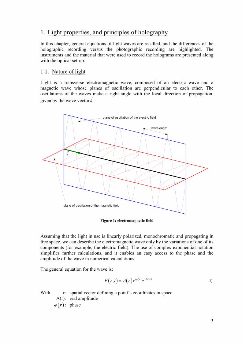
Light is a transverse electromagnetic wave, composed of an electric wave and a
magnetic wave whose planes of oscillation are perpendicular to each other. The
oscillations of the waves make a right angle with the local direction of propagation,
given by the wave vector k�
.
wavelength
k
plane of oscillation of the magnetic field
plane of oscillation of the electric field
Figure 1: electromagnetic field
Assuming that the light in use is linearly polarized, monochromatic and propagating in
free space, we can describe the electromagnetic wave only by the variations of one of its
components (for example, the electric field). The use of complex exponential notation
simplifies further calculations, and it enables an easy access to the phase and the
amplitude of the wave in numerical calculations.
The general equation for the wave is:
( ) ( ) ( ) 2, i r i tE r t A r e eϕ π ν−= 1)
With r: spatial vector defining a point’s coordinates in space
A(r): real amplitude
( )rϕ : phase
4
ν: frequency of light, c
νλ
= (λ being the wavelength and c the light speed)
t: time
This equation depends both on space (r) and time (t), however when using
monochromatic light the temporal part is omitted, because interferences of waves with a
sharp, single frequency are stable in time. In the real case a light source is not emitting
in only one single frequency, however if the bandwidth is narrow enough (such as for
laser light), this approximation still holds. Thus for the following, we consider light as
being described by the complex amplitude:
( ) ( ) ( )i rV r A r e ϕ= 2)
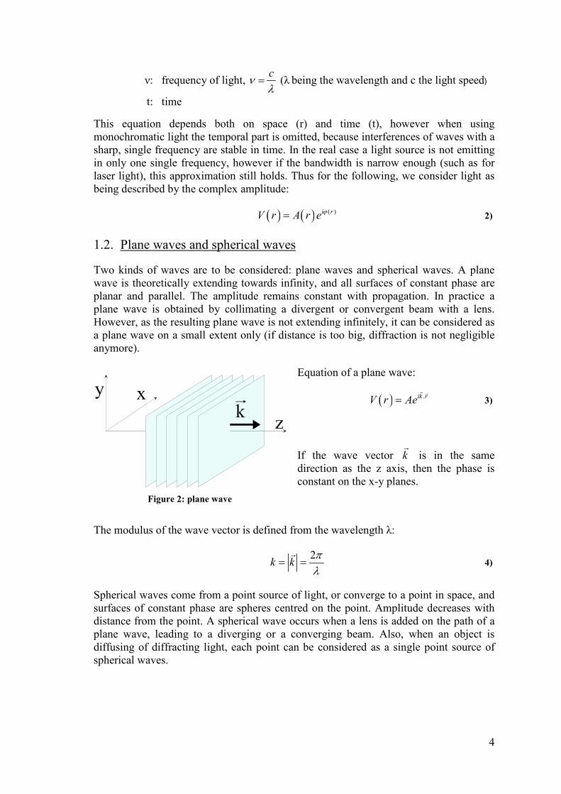
1.2. Plane waves and spherical waves
Two kinds of waves are to be considered: plane waves and spherical waves. A plane
wave is theoretically extending towards infinity, and all surfaces of constant phase are
planar and parallel. The amplitude remains constant with propagation. In practice a
plane wave is obtained by collimating a divergent or convergent beam with a lens.
However, as the resulting plane wave is not extending infinitely, it can be considered as
a plane wave on a small extent only (if distance is too big, diffraction is not negligible
anymore).
Equation of a plane wave:
( ) .ik rV r Ae=� �
3)
If the wave vector k�
is in the same
direction as the z axis, then the phase is
constant on the x-y planes.
The modulus of the wave vector is defined from the wavelength λ:
2
k kπλ
= =�
4)
Spherical waves come from a point source of light, or converge to a point in space, and
surfaces of constant phase are spheres centred on the point. Amplitude decreases with
distance from the point. A spherical wave occurs when a lens is added on the path of a
plane wave, leading to a diverging or a converging beam. Also, when an object is
diffusing of diffracting light, each point can be considered as a single point source of
spherical waves.
xy
zk
Figure 2: plane wave
5
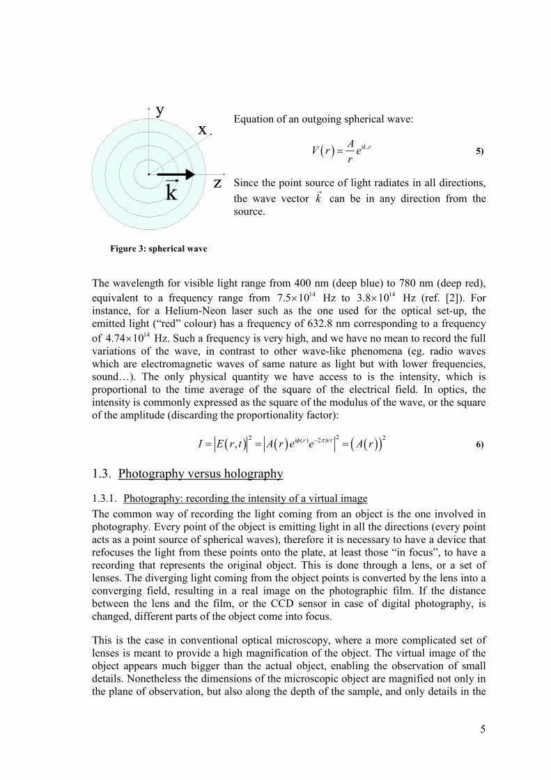
Equation of an outgoing spherical wave:
( ) .ik rAV r e
r= 5)
Since the point source of light radiates in all directions,
the wave vector k�
can be in any direction from the
source.
The wavelength for visible light range from 400 nm (deep blue) to 780 nm (deep red),
equivalent to a frequency range from 147.5 10× Hz to 143.8 10× Hz (ref. [2]). For
instance, for a Helium-Neon laser such as the one used for the optical set-up, the
emitted light (“red” colour) has a frequency of 632.8 nm corresponding to a frequency
of 144.74 10× Hz. Such a frequency is very high, and we have no mean to record the full
variations of the wave, in contrast to other wave-like phenomena (eg. radio waves
which are electromagnetic waves of same nature as light but with lower frequencies,
sound…). The only physical quantity we have access to is the intensity, which is
proportional to the time average of the square of the electrical field. In optics, the
intensity is commonly expressed as the square of the modulus of the wave, or the square
of the amplitude (discarding the proportionality factor):
( ) ( ) ( )( )22 2( ) 2, i r i tI E r t A r e e A rφ π ν−= = = 6)
1.3. Photography versus holography
1.3.1. Photography: recording the intensity of a virtual image
The common way of recording the light coming from an object is the one involved in
photography. Every point of the object is emitting light in all the directions (every point
acts as a point source of spherical waves), therefore it is necessary to have a device that
refocuses the light from these points onto the plate, at least those “in focus”, to have a
recording that represents the original object. This is done through a lens, or a set of
lenses. The diverging light coming from the object points is converted by the lens into a
converging field, resulting in a real image on the photographic film. If the distance
between the lens and the film, or the CCD sensor in case of digital photography, is
changed, different parts of the object come into focus.
This is the case in conventional optical microscopy, where a more complicated set of
lenses is meant to provide a high magnification of the object. The virtual image of the
object appears much bigger than the actual object, enabling the observation of small
details. Nonetheless the dimensions of the microscopic object are magnified not only in
the plane of observation, but also along the depth of the sample, and only details in the
Figure 3: spherical wave
6
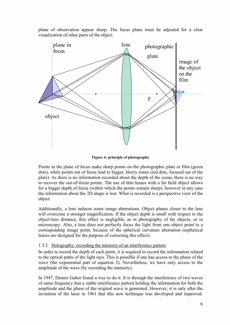
plane of observation appear sharp. The focus plane must be adjusted for a clear
visualization of other parts of the object.
plane in focus
lens
object
image of the object on the film
F
photographic
plate
Figure 4: principle of photography
Points in the plane of focus make sharp points on the photographic plate or film (green
dots), while points out of focus lead to bigger, blurry zones (red dots, focused out of the
plate). As there is no information recorded about the depth of the scene, there is no way
to recover the out-of-focus points. The use of thin lenses with a far field object allows
for a bigger depth of focus (within which the points remain sharp), however in any case
the information about the 3D shape is lost. What is recorded is a perspective view of the
object.
Additionally, a lens induces some image aberrations. Object planes closer to the lens
will overcome a stronger magnification. If the object depth is small with respect to the
object-lens distance, this effect is negligible, as in photography of far objects, or in
microscopy. Also, a lens does not perfectly focus the light from one object point to a
corresponding image point, because of the spherical curvature aberration (aspherical
lenses are designed for the purpose of correcting this effect).
1.3.2. Holography: recording the intensity of an interference pattern
In order to record the depth of each point, it is required to record the information related
to the optical paths of the light rays. This is possible if one has access to the phase of the
wave (the exponential part of equation 2). Nevertheless, we have only access to the
amplitude of the wave (by recording the intensity).
In 1947, Dennis Gabor found a way to do it. It is through the interference of two waves
of same frequency that a stable interference pattern holding the information for both the
amplitude and the phase of the original wave is generated. However, it is only after the
invention of the laser in 1961 that this new technique was developed and improved.
7
Indeed the process involves the use of a highly coherent light source, and only laser
light provides this property. Temporal coherence, related to the stability of the emitted
wavelength and the sharpness of the output bandwidth, is a requirement in order to have
a stable and contrasted pattern. The coherence length, in relation with the temporal
coherence, is a limit to a scene depth. Light beams travelling along different optical
paths can interfere only if the optical path difference is less than the coherence length.
This is due to the need of temporal synchronization between the interfering waves. The
lasers in common use in the laboratories offer coherence lengths ranging from several
centimetres to several meters, which is enough for digital holographic microscopy.
Spatial coherence is linked to the light source dimensions. In the case of a spherical
wave, the smaller the light source, the better the spatial coherence. If the source is
extending in space, the difference in the optical paths will lead to a phase shift between
the different “beams” coming from the source points, and the phase will not be constant
through the output beam. While the temporal coherence is about the synchronization of
the wave in the longitudinal direction, the spatial coherence measures the
synchronization across the beam.
Another critical parameter while recording holograms is stability. The exposure time
can be rather long when photographic plates are used, because the high resolution
recording plates have a lower sensibility, and exposure time of several seconds are
common. Also the recorded light is much dimmer than in photography, because it is not
focused on the plate with a lens. It is the whole optical field from the object that
interacts with a reference field instead, leading to very small interference fringes, down
to half a wavelength. Any vibration in the system of a magnitude higher than this
amount will lead to a shift of the fringes during the exposure, and the contrast will
decrease, or no pattern at all will be recorded.
Digital recording of holograms enables to reduce stability problems related to the
exposure time, in particular due to vibrations, since the holograms can be recorded
within a fraction of a second. Still, a high degree of coherence is a critical requirement.
The phase shifting technique presented in the chapter 5 requires a high stability too,
because the recording of several holograms with different phase shifts takes some time.
object beam
reference beam
interferences at the
holographic plate
Laserbeam splitter
expansion and/or
collimation of
the beam
object
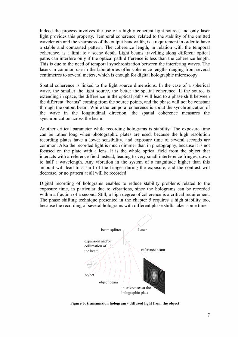
Figure 5: transmission hologram - diffused light from the object
8
Figure 5 shows the principle for the making of a transmission hologram. Two beams of
coherent light interfere on the holographic plate (or the CCD sensor, for digital
holography). One comes directly from the laser, the second one is modulated by the
object (in this example, it is the light diffused by the object). Since coherence between
the beams is necessary as explained before, the two beams come from the same source
of light, a laser. A beam splitter separates the two beams. The example above shows an
off-axis set-up (the object beam and the reference beam are not aligned).
From a qualitative point of view, the interference pattern comes from the destructive
and constructive addition of the two waves. When two wave crests coincide,
constructive interference leads to a higher amplitude (and higher recorded intensity),
and when a crest is present at the same place as a trough, destructive interference occurs
and a minimum of intensity is recorded. Between these two extremes, partial
interference is responsible for the smooth appearance of the interference fringes. This is
the general case, where the two interfering waves do not have necessarily the same
amplitude. Of course light waves also vary in time, but due to the use of a highly
monochromatic and coherent source, the phase shifts between object beam and
reference beam remain constant for each point of the hologram, and the intensity pattern
is constant in time.
When superimposing two beams, the waves add together:
( ) ( ) ( ), , ,H O RV x y V x y V x y= + 7)
Where ( ),HV x y is the complex amplitude of the hologram, and ( ),OV x y and ( ),RV x y
are the complex amplitudes of the object beam and the reference beam respectively.
The resulting intensity is proportional to the square of the modulus of the field at the
plane of the holographic plate (ref. [1] & [2]):
( ) ( ) ( )
( ) ( ) ( ) ( ) ( ) ( ) ( )
2
2 2 * *
, , ,
, , , , , , ,
H O R
H O R O R R O
I x y V x y V x y
I x y V x y V x y V x y V x y V x y V x y
= +
= + + + 8)
( ) ( ) ( ) ( ) ( ) ( ) ( )( ), , , 2 , , cos , ,H O R O H R OI x y I x y I x y I x y I x y x y x yϕ ϕ= + + − 9)
The intensity of light is recorded either chemically when the hologram is made on a
photographic plate, or electronically with a CCD sensor (and the corresponding electric
signals are sampled and quantized for saving the data in a digital format). The
corresponding photographic plate transparency after development is proportional to the
original intensity distribution:
0( , ) ( , )H Hx y I x yτ τ β= + 10)
where 0τ is the mean transparency and β is a proportionality factor (depending on
sensibility, time exposure…). 0β < for a negative of the plate.
While the silver halide plates are not fully linear (but they are considered linear on a
certain range), a CCD sensor is fully linear below saturation. In this case the offset 0τ is
9
called the “black level”, and β depends on the selected exposure time and sensitivity.
Thanks to this linearity, the equations for the intensity can be used to describe what
happens during the reconstruction.
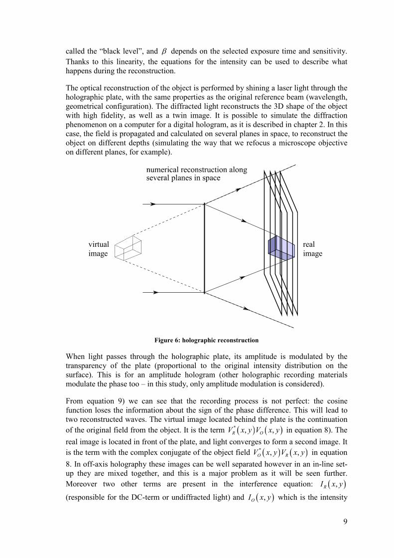
The optical reconstruction of the object is performed by shining a laser light through the
holographic plate, with the same properties as the original reference beam (wavelength,
geometrical configuration). The diffracted light reconstructs the 3D shape of the object
with high fidelity, as well as a twin image. It is possible to simulate the diffraction
phenomenon on a computer for a digital hologram, as it is described in chapter 2. In this
case, the field is propagated and calculated on several planes in space, to reconstruct the
object on different depths (simulating the way that we refocus a microscope objective
on different planes, for example).
Figure 6: holographic reconstruction
When light passes through the holographic plate, its amplitude is modulated by the
transparency of the plate (proportional to the original intensity distribution on the
surface). This is for an amplitude hologram (other holographic recording materials
modulate the phase too – in this study, only amplitude modulation is considered).
From equation 9) we can see that the recording process is not perfect: the cosine
function loses the information about the sign of the phase difference. This will lead to
two reconstructed waves. The virtual image located behind the plate is the continuation
of the original field from the object. It is the term ( ) ( )* , ,R OV x y V x y in equation 8). The
real image is located in front of the plate, and light converges to form a second image. It
is the term with the complex conjugate of the object field ( ) ( )* , ,O RV x y V x y in equation
8. In off-axis holography these images can be well separated however in an in-line set-
up they are mixed together, and this is a major problem as it will be seen further.
Moreover two other terms are present in the interference equation: ( ),RI x y
(responsible for the DC-term or undiffracted light) and ( ),OI x y which is the intensity
virtual
image
real
image
10
of the object alone (also called object auto-interference). These two terms can be easily
removed from the hologram in numerical calculation.
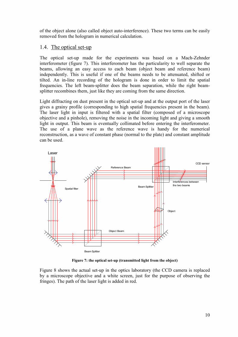
1.4. The optical set-up
The optical set-up made for the experiments was based on a Mach-Zehnder
interferometer (figure 7). This interferometer has the particularity to well separate the
beams, allowing an easy access to each beam (object beam and reference beam)
independently. This is useful if one of the beams needs to be attenuated, shifted or
tilted. An in-line recording of the hologram is done in order to limit the spatial
frequencies. The left beam-splitter does the beam separation, while the right beam-
splitter recombines them, just like they are coming from the same direction.
Light diffracting on dust present in the optical set-up and at the output port of the laser
gives a grainy profile (corresponding to high spatial frequencies present in the beam).
The laser light in input is filtered with a spatial filter (composed of a microscope
objective and a pinhole), removing the noise in the incoming light and giving a smooth
light in output. This beam is eventually collimated before entering the interferometer.
The use of a plane wave as the reference wave is handy for the numerical
reconstruction, as a wave of constant phase (normal to the plate) and constant amplitude
can be used.
Figure 7: the optical set-up (transmitted light from the object)
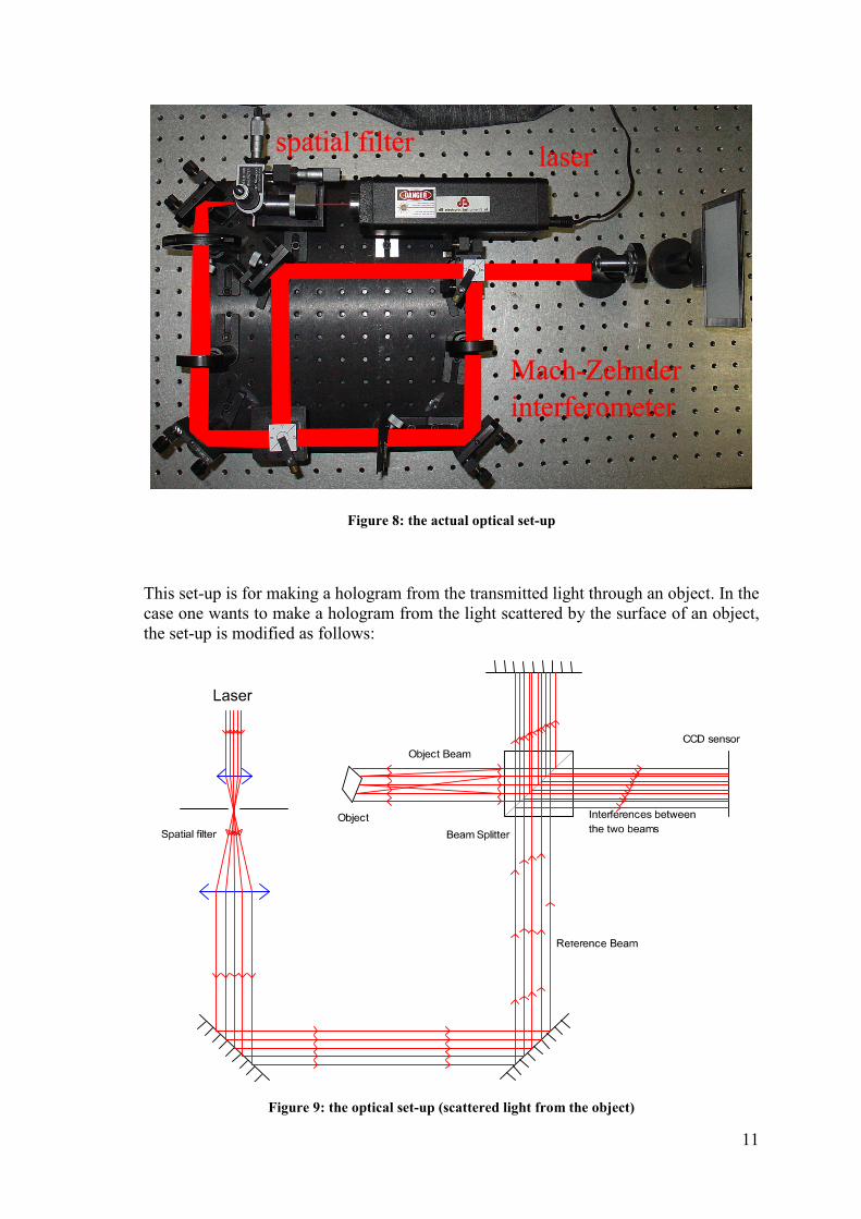
Figure 8 shows the actual set-up in the optics laboratory (the CCD camera is replaced
by a microscope objective and a white screen, just for the purpose of observing the
fringes). The path of the laser light is added in red.
11
Figure 8: the actual optical set-up
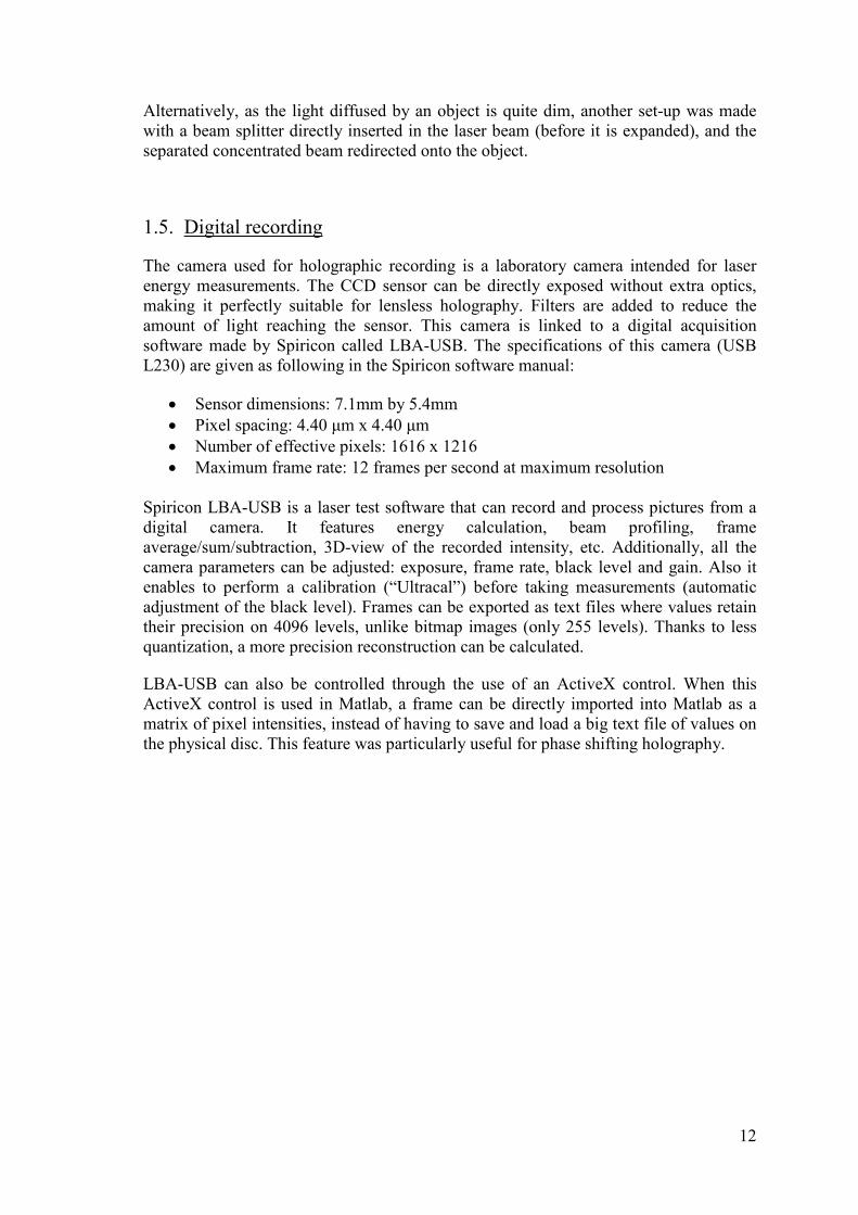
This set-up is for making a hologram from the transmitted light through an object. In the
case one wants to make a hologram from the light scattered by the surface of an object,
the set-up is modified as follows:
Figure 9: the optical set-up (scattered light from the object)
12
Alternatively, as the light diffused by an object is quite dim, another set-up was made
with a beam splitter directly inserted in the laser beam (before it is expanded), and the
separated concentrated beam redirected onto the object.
1.5. Digital recording
The camera used for holographic recording is a laboratory camera intended for laser
energy measurements. The CCD sensor can be directly exposed without extra optics,
making it perfectly suitable for lensless holography. Filters are added to reduce the
amount of light reaching the sensor. This camera is linked to a digital acquisition
software made by Spiricon called LBA-USB. The specifications of this camera (USB
L230) are given as following in the Spiricon software manual:
• Sensor dimensions: 7.1mm by 5.4mm
• Pixel spacing: 4.40 µm x 4.40 µm
• Number of effective pixels: 1616 x 1216
• Maximum frame rate: 12 frames per second at maximum resolution
Spiricon LBA-USB is a laser test software that can record and process pictures from a
digital camera. It features energy calculation, beam profiling, frame
average/sum/subtraction, 3D-view of the recorded intensity, etc. Additionally, all the
camera parameters can be adjusted: exposure, frame rate, black level and gain. Also it
enables to perform a calibration (“Ultracal”) before taking measurements (automatic
adjustment of the black level). Frames can be exported as text files where values retain
their precision on 4096 levels, unlike bitmap images (only 255 levels). Thanks to less
quantization, a more precision reconstruction can be calculated.
LBA-USB can also be controlled through the use of an ActiveX control. When this
ActiveX control is used in Matlab, a frame can be directly imported into Matlab as a
matrix of pixel intensities, instead of having to save and load a big text file of values on
the physical disc. This feature was particularly useful for phase shifting holography.
13
2. Reconstruction methods
For the reconstruction of the image, we will assume that the hologram is only
modulating the amplitude of the incident light, and that there is no modulation of the
phase in x and y (plane of the hologram). When the light passes through a transparent
slide of constant thickness with a varying transmittance, it diffracts and higher spatial
frequencies are created. In optics, the spatial frequency is related to the angle of the
propagating direction with respect to the plate normal. All the diffracted waves interfere
together, and converge towards the image points.
2.1. Decomposition in spherical waves
An intuitive way to consider the diffraction phenomenon is to consider each point of the
diffracting object as a single emitter of light. This principle was thought about as early
as 1678 by Christiaan Huygens, stating that the propagated form of a wave front can be
found from the sum of all the spherical waves originating at the previous wave front.
In the case of a hologram, every point at the surface is considered as a point source of
light, with same phase as the reconstructing beam impinging on the surface at that point,
and having for amplitude the product of the amplitude of the reconstructing beam with
the transparency value at that point. If the recording media is linear, then the
transparency of the corresponding point is directly proportional to the intensity of the
interferences in equations 8 and 9.
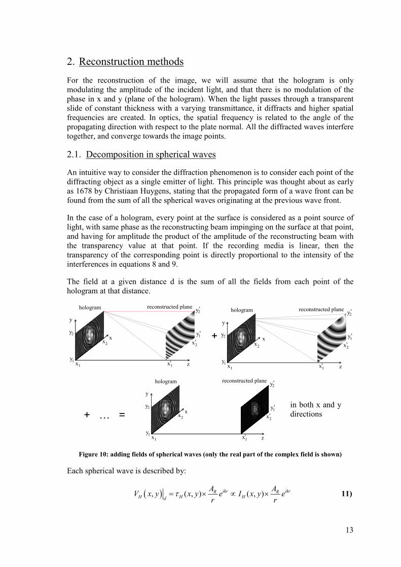
The field at a given distance d is the sum of all the fields from each point of the
hologram at that distance.
xy
1'
2x
1
y2
x1
2
y1
y2
'x
'
'hologram reconstructed plane
y
x
z xy
1'
2x
1
y2
x1
2
y1
y2
'x
'
'hologram reconstructed plane
z
y
x
xy
1'
2x
1
y2
x1
2
y1
y2
'x
'
'hologram reconstructed plane
y
x
z
Figure 10: adding fields of spherical waves (only the real part of the complex field is shown)
Each spherical wave is described by:
( ), ( , ) ( , )ikr ikrR RH H Hd
A AV x y x y e I x y e
r rτ= × ∝ × 11)
+
+ … = in both x and y
directions
14
With ( ) ( )2 2 2' 'r x x y y d= − + − + (optical path between a point of the hologram and a
point of the reconstructed plane at the distance d).
Or, from the reconstructed plane point of view, the field for each point at distance d is
the sum of the fields from all the points of the hologram with phase and amplitude
affected by the propagated distance r:
( )2 2
1 1
', ' ( , )
x y
ikrRd H
x y
AV x y I x y e dxdy
r= ∫ ∫ 12)
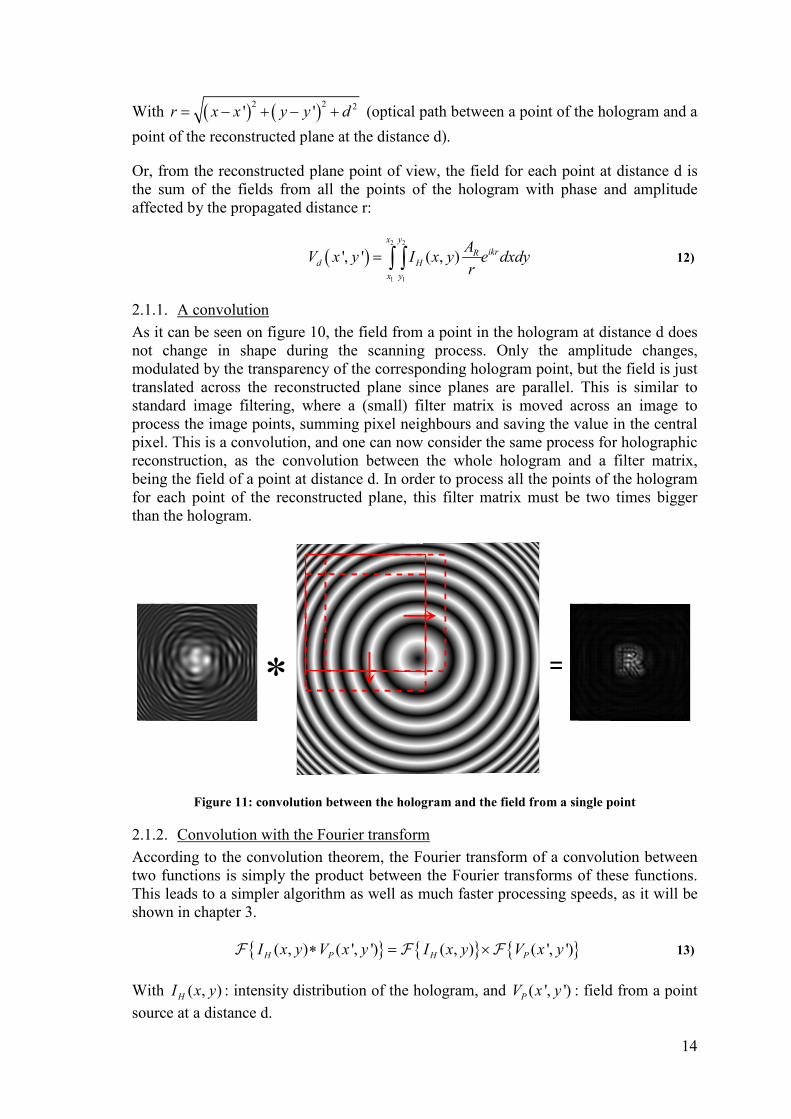
2.1.1. A convolution
As it can be seen on figure 10, the field from a point in the hologram at distance d does
not change in shape during the scanning process. Only the amplitude changes,
modulated by the transparency of the corresponding hologram point, but the field is just
translated across the reconstructed plane since planes are parallel. This is similar to
standard image filtering, where a (small) filter matrix is moved across an image to
process the image points, summing pixel neighbours and saving the value in the central
pixel. This is a convolution, and one can now consider the same process for holographic
reconstruction, as the convolution between the whole hologram and a filter matrix,
being the field of a point at distance d. In order to process all the points of the hologram
for each point of the reconstructed plane, this filter matrix must be two times bigger
than the hologram.
=
Figure 11: convolution between the hologram and the field from a single point
2.1.2. Convolution with the Fourier transform
According to the convolution theorem, the Fourier transform of a convolution between
two functions is simply the product between the Fourier transforms of these functions.
This leads to a simpler algorithm as well as much faster processing speeds, as it will be
shown in chapter 3.
{ } { } { }( , ) ( ', ') ( , ) ( ', ')H P H PI x y V x y I x y V x y∗ = ×F F F 13)
With ( , )HI x y : intensity distribution of the hologram, and ( ', ')PV x y : field from a point
source at a distance d.
15
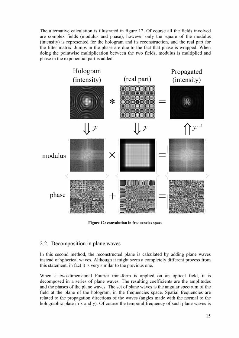
The alternative calculation is illustrated in figure 12. Of course all the fields involved
are complex fields (modulus and phase), however only the square of the modulus
(intensity) is represented for the hologram and its reconstruction, and the real part for
the filter matrix. Jumps in the phase are due to the fact that phase is wrapped. When
doing the pointwise multiplication between the two fields, modulus is multiplied and
phase in the exponential part is added.
(real part)(intensity) (intensity)
Hologram Propagated
F F F-1
modulus
phase
Figure 12: convolution in frequencies space
2.2. Decomposition in plane waves
In this second method, the reconstructed plane is calculated by adding plane waves
instead of spherical waves. Although it might seem a completely different process from
this statement, in fact it is very similar to the previous one.
When a two-dimensional Fourier transform is applied on an optical field, it is
decomposed in a series of plane waves. The resulting coefficients are the amplitudes
and the phases of the plane waves. The set of plane waves is the angular spectrum of the
field at the plane of the hologram, in the frequencies space. Spatial frequencies are
related to the propagation directions of the waves (angles made with the normal to the
holographic plate in x and y). Of course the temporal frequency of such plane waves is
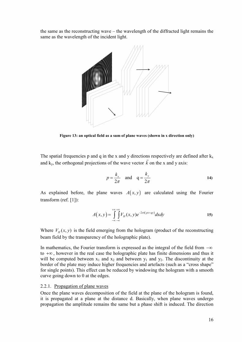
16
the same as the reconstructing wave – the wavelength of the diffracted light remains the
same as the wavelength of the incident light.
Figure 13: an optical field as a sum of plane waves (shown in x direction only)
The spatial frequencies p and q in the x and y directions respectively are defined after kx
and ky, the orthogonal projections of the wave vector k�
on the x and y axis:
and q2 2
yxkk
pπ π
= = 14)
As explained before, the plane waves ( ),A x y are calculated using the Fourier
transform (ref. [1]):
( ) ( )2, ( , )
i px qy
HA x y V x y e dxdyπ
+∞ +∞− +
−∞ −∞
= ∫ ∫ 15)
Where ( , )HV x y is the field emerging from the hologram (product of the reconstructing
beam field by the transparency of the holographic plate).
In mathematics, the Fourier transform is expressed as the integral of the field from −∞
to +∞ , however in the real case the holographic plate has finite dimensions and thus it
will be computed between x1 and x2 and between y1 and y2. The discontinuity at the
border of the plate may induce higher frequencies and artefacts (such as a “cross shape”
for single points). This effect can be reduced by windowing the hologram with a smooth
curve going down to 0 at the edges.
2.2.1. Propagation of plane waves
Once the plane waves decomposition of the field at the plane of the hologram is found,
it is propagated at a plane at the distance d. Basically, when plane waves undergo
propagation the amplitude remains the same but a phase shift is induced. The direction
17
of propagation is along the z axis, normal to the plane of the hologram. The added phase
shift is created by the scalar product .k r� �
in equation 3.
( ) ( ). , , . 0,0, .x y z zk r k k k d k d= =� �
16)
And with 2 2 2
x y zk k k k= + + :
( ) ( )2
2 22 2 2 2. . 2 2 . 2x yk r k k k d p q d md
ππ π π
λ = − − = − − =
� � 17)
2 2
2
1m p q
λ= − − is the propagation coefficient and is different for each plane wave.
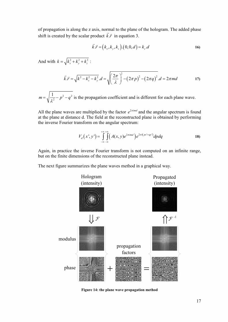
All the plane waves are multiplied by the factor 2 imde π and the angular spectrum is found
at the plane at distance d. The field at the reconstructed plane is obtained by performing
the inverse Fourier transform on the angular spectrum:
( ) ( ) ( )2 ' '2', ' ( , )i px qyimd
dV x y A x y e e dpdqππ
+∞ +∞+
−∞ −∞
= ∫ ∫ 18)
Again, in practice the inverse Fourier transform is not computed on an infinite range,
but on the finite dimensions of the reconstructed plane instead.
The next figure summarizes the plane waves method in a graphical way.
(intensity) (intensity)
Hologram Propagated
F F-1
modulus
phase
propagation
factors
Figure 14: the plane wave propagation method
18
The plane waves method is therefore very similar to the convolution method with the
Fourier transform. One Fourier transform is avoided (from the point source field to its
Fourier transform), consequently a faster processing speed is expected.
2.2.2. Space sampling and frequencies sampling
When the hologram is recorded on a CCD sensor, it is sampled in space. Light
impinging on the CCD sensor is integrated on the pixel surface. For numerical
calculations, sampled values are assumed to be sampled points separated by the
sampling distance S. For a CCD sensor, this is the pixel size, of the inter-pixel distance.
The latter is a better description since the pixel surface does not necessarily take the
entire surface available between pixels, due to the presence of transfer registers or
shielding gates, channel stops…
The Shannon-Nyquist sampling theorem states that when the Fourier transform is
calculated on a sampled signal, the maximum frequency in the signal should be below
half of the sampling frequency. For this reason, the Fast Fourier Transform algorithm
(FFT) calculates the frequencies between –Fmax and +Fmax. Spatial frequencies higher
than this value will be folded back into the limited frequency range, therefore a limit on
spatial frequencies has to be set, as it will be demonstrated in chapter 3.
Just as the spatial signal is sampled in space, its frequential counterpart is sampled in
the frequencies space. The frequencies sampling depends both on the maximum
frequency in the signal (linked to the spatial sampling value) and on the number of
samples along this dimension.
The USB L230 camera has a sampling value of 4.4 µm, therefore the sampling
frequency is:
5 -1
6
12.27 10 m
4.4 10SF −= ≈ ×
×
and the maximum spatial frequency is:
5 -1
max 1.14 10 m2
SFF = = × .
The FFT algorithm is optimized for sampled signals dimensions being a power of 2.
The matrix to be processed is padded with zeros up to the next power of 2. For the
camera resolution (1616 x 1216), this leads to a matrix of 2048 x 2048 values.
The output of the FFT function is in the following form (frequencies indexes, shown for
one dimension only):
0 F1 F2 … Fmax-2 Fmax-1 ± Fmax - Fmax-1 - Fmax-2 … - F2 - F1
The frequencies sampling is thus 2 -1max 1.11 10 m1024
samp
FF = ≈ ×
2048 values
1025 values
19
3. Physical limitations, magnification
3.1. Object to plate distance
3.1.1. Absolute minimum distance
In digital holography, the hologram is recorded on a CCD sensor, and is sampled in x
and y directions. Care must be taken not to have frequencies higher than the sampling
frequency in the sampled signal (the intensity interference pattern).
According to the Shannon-Nyquist sampling theorem, a signal must be sampled at a
frequency at least two times higher than the highest frequency present in the signal, or
at least two times a period.
In the case of recording an interference pattern between a plane wave and a spherical
wave from a point source at distance d (simplest hologram of one point), the higher the
angle between the optical path to a point on the plate and the orthogonal projection of
the point on the plate, the smaller the distance between the fringes. The fringes appear
to shrink with the increasing lateral distance. This is a Fresnel zone plate pattern.
As long as the optical path difference between two adjacent samples is less than half a
wavelength, the phase difference remains below π and it is possible to record the
pattern. This comes from the spherical wave equation:
( ) ( )
1
1
112
2
1
2
2 1
2 2 2
1 2
1 1 1
,2
ikr
O
i r ri krikr
O
V e with kr
V e e e with r r rr r r
if r
πϕλ
πλ
λϕ π
+∆ +∆
= =
= = = = + ∆
∆ ≤ ∆ ≤
19)
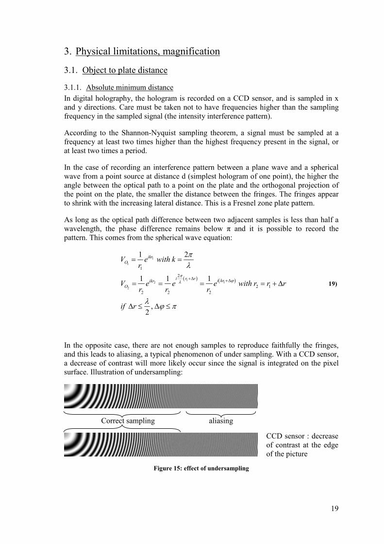
In the opposite case, there are not enough samples to reproduce faithfully the fringes,
and this leads to aliasing, a typical phenomenon of under sampling. With a CCD sensor,
a decrease of contrast will more likely occur since the signal is integrated on the pixel
surface. Illustration of undersampling:
Correct sampling aliasing
Figure 15: effect of undersampling
CCD sensor : decrease
of contrast at the edge
of the picture
20
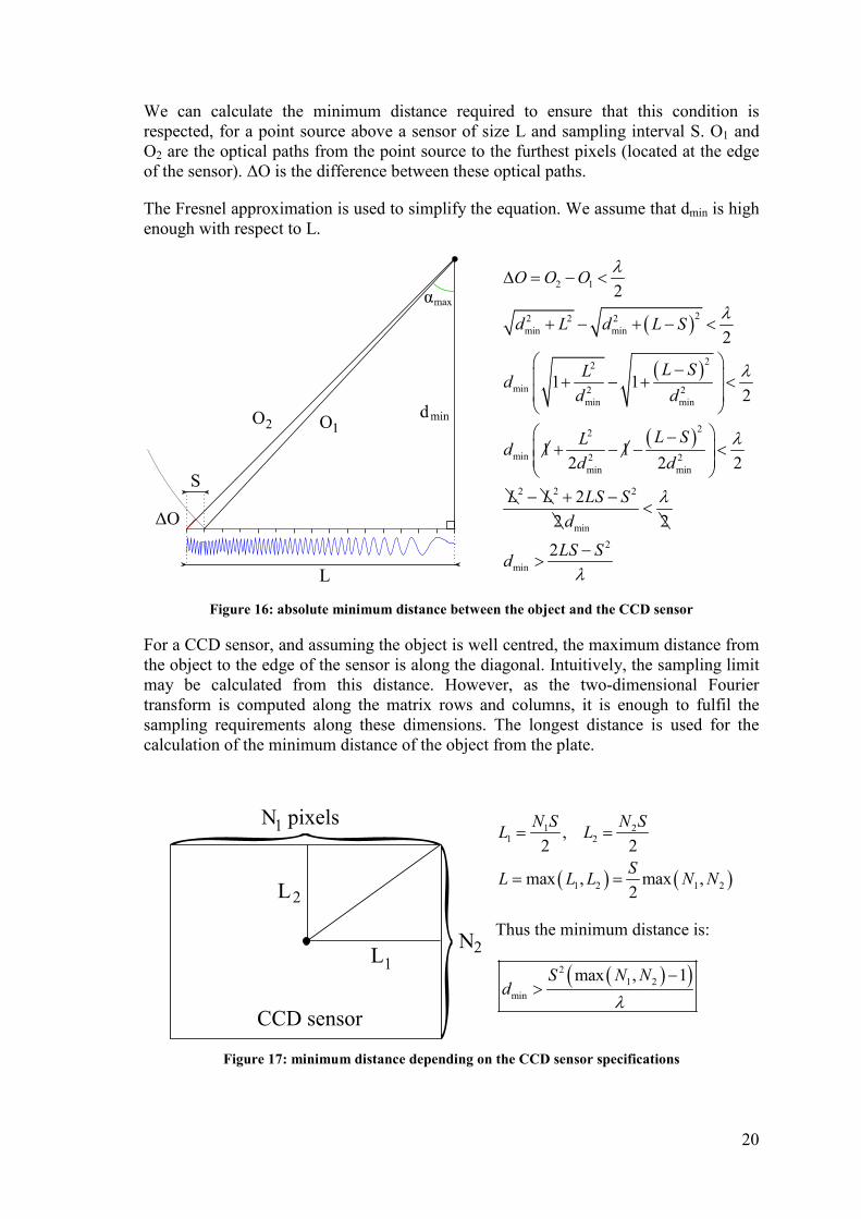
We can calculate the minimum distance required to ensure that this condition is
respected, for a point source above a sensor of size L and sampling interval S. O1 and
O2 are the optical paths from the point source to the furthest pixels (located at the edge
of the sensor). ∆O is the difference between these optical paths.
The Fresnel approximation is used to simplify the equation. We assume that dmin is high
enough with respect to L.
( )
( )
( )
2 1
22 2 2
min min
22
min 2 2
min min
22
min 2 2
min min
2 2 2
min
2
min
2
2
1 12
1 12 2 2
2
2 2
2
O O O
d L d L S
L SLd
d d
L SLd
d d
L L LS S
d
LS Sd
λ
λ
λ
λ
λ
λ
∆ = − <
+ − + − <
− + − + <
−+ − − <
− + −<
−>
Figure 16: absolute minimum distance between the object and the CCD sensor
For a CCD sensor, and assuming the object is well centred, the maximum distance from
the object to the edge of the sensor is along the diagonal. Intuitively, the sampling limit
may be calculated from this distance. However, as the two-dimensional Fourier
transform is computed along the matrix rows and columns, it is enough to fulfil the
sampling requirements along these dimensions. The longest distance is used for the
calculation of the minimum distance of the object from the plate.
( ) ( )
1 21 2
1 2 1 2
,2 2
max , max ,2
N S N SL L
SL L L N N
= =
= =
Thus the minimum distance is:
( )( )2
1 2
min
max , 1S N Nd
λ
−>
Figure 17: minimum distance depending on the CCD sensor specifications
21
Alternatively, we can define the maximum angle for the light impinging on the sensor:
( )( )
( )( )( )( )
1 21 2
max 2
min 1 21 2
max , max ,2tan2 max , 1 2max , 1
SN N N NL
d S N N SS N N
λ λ λα
= = = ≈ −−
max Arctan2S
λα =
With the following parameters:
6 9
1 24.4 10 , 1616 , 1216 , 632.8 10S m N pixels N pixels mλ− −= × = = = ×
We find an absolute minimum distance of min 49.4d mm≈ , and a maximum angle
object beam angle of max 4.1α ≈ ° .
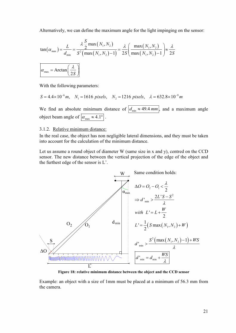
3.1.2. Relative minimum distance:
In the real case, the object has non negligible lateral dimensions, and they must be taken
into account for the calculation of the minimum distance.
Let us assume a round object of diameter W (same size in x and y), centred on the CCD
sensor. The new distance between the vertical projection of the edge of the object and
the furthest edge of the sensor is L’.
Same condition holds:
( )( )
2 1
2
min
1 2
2
2 ''
'2
1' max ,
2
O O O
L S Sd
Wwith L L
L S N N W
λ
λ
∆ = − <
−⇒ >
= +
= +
( )( )2
1 2
min
min min
max , 1'
'
S N N WSd
WSd d
λ
λ
− +>
= +
Figure 18: relative minimum distance between the object and the CCD sensor
Example: an object with a size of 1mm must be placed at a minimum of 56.3 mm from
the camera.
22
3.2. Maximum achievable resolution
The resolution is the ability to distinguish between two distinct points. As the
information is distributed in the hologram, and the waves are “refocused” in space, the
object may have a higher achievable resolution than the plate sampling value,
depending on the geometric configuration.
In the book from Thomas Kreis, “Handbook of Holographic Interferometry” (ref. [3],
page 171), a simple approximation is given to evaluate the maximum resolution
achieved by a holographic microscopy system. It is given by the formula: 0.61d
H
λδ ∼
With d being the distance of the object from the hologram, and H the dimension of the
CCD sensor. As we want the smallest possible resolution, let us take the distance limit
previously calculated, and the largest dimension of the CCD sensor (along the x axis):
9 36
6
632.8 10 49.4 100.61 2.68 10 m
4.4 10 1616δ
− −−
−
× × ×= × ≈ ×
× ×
A maximum lateral resolution of 2.7 µm is expected, which means that object points
separated by a smaller distance will appear as a unique point. This distance is higher
than the theoretical limit due to the light wavelength (diffraction limit).
Other formula are given in the same book, but for different set-ups, in particular for the
case of a Fourier hologram, where the reference beam is a point source of spherical
waves located in the plane of the hologram, which enlarges the interference fringes and
consequently lowers the distance limit from the hologram. However this set-up was not
used in this project.
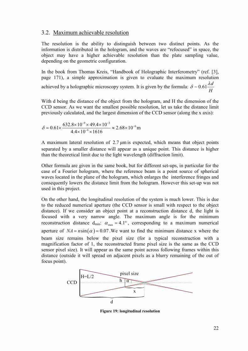
On the other hand, the longitudinal resolution of the system is much lower. This is due
to the reduced numerical aperture (the CCD sensor is small with respect to the object
distance). If we consider an object point at a reconstruction distance d, the light is
focused with a very narrow angle. The maximum angle is for the minimum
reconstruction distance dmin: max 4.1α = ° , corresponding to a maximum numerical
aperture of ( )sin 0.07NA n α= = .We want to find the minimum distance x where the
beam size remains below the pixel size (for a typical reconstruction with a
magnification factor of 1, the reconstructed frame pixel size is the same as the CCD
sensor pixel size). It will appear as the same point across following frames within this
distance (outside it will spread on adjacent pixels as a blurry remaining of the out of
focus point).
Figure 19: longitudinal resolution
23
( ) / 2tan
/ 2
H h hd S d S dx
d x H L N Sα
× ×= = ⇒ = = =
× 20)
With d = 49.4mm and N = 1616 pixels: 30.6 µmx = , which means that frames
separated by less than this distance will not show more detail in depth. Moreover, this
distance increases with the reconstruction distance, since the angle gets narrower.
Holograms will be reconstructed at the same resolution as the CCD sensor. If a higher
resolution is expected in the reconstructed frames, then it is necessary to implement a
magnification technique, or find a way to supersample the reconstructed image.
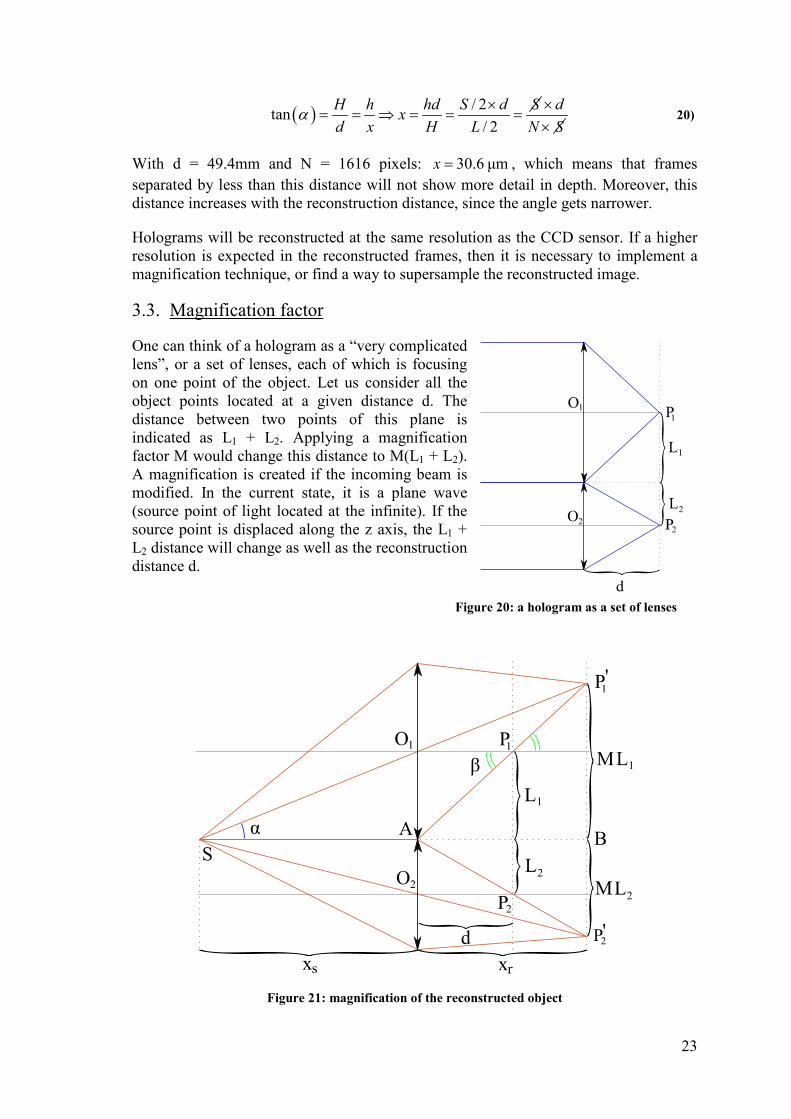
3.3. Magnification factor
One can think of a hologram as a “very complicated
lens”, or a set of lenses, each of which is focusing
on one point of the object. Let us consider all the
object points located at a given distance d. The
distance between two points of this plane is
indicated as L1 + L2. Applying a magnification
factor M would change this distance to M(L1 + L2).
A magnification is created if the incoming beam is
modified. In the current state, it is a plane wave
(source point of light located at the infinite). If the
source point is displaced along the z axis, the L1 +
L2 distance will change as well as the reconstruction
distance d.
Figure 21: magnification of the reconstructed object
Figure 20: a hologram as a set of lenses
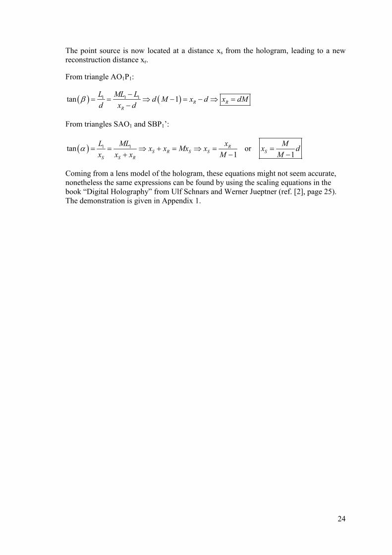
24
The point source is now located at a distance xs from the hologram, leading to a new
reconstruction distance xr.
From triangle AO1P1:
( ) ( )1 1 1tan 1 R R
R
L ML Ld M x d x dM
d x dβ
−= = ⇒ − = − ⇒ =
−
From triangles SAO1 and SBP1’:
( ) 1 1tan or1 1
RS R S S S
S S R
L ML x Mx x Mx x x d
x x x M Mα = = ⇒ + = ⇒ = =
+ − −
Coming from a lens model of the hologram, these equations might not seem accurate,
nonetheless the same expressions can be found by using the scaling equations in the
book “Digital Holography” from Ulf Schnars and Werner Jueptner (ref. [2], page 25).
The demonstration is given in Appendix 1.
25
4. Implementation in Matlab and results analysis
The virtual holographic reconstruction was implemented with Matlab. The reasons for
this choice are numerous. Firstly Matlab is designed and optimized to process matrices,
and the data to process was in the form of 2D matrices (hologram, single frames) or 3D
matrices (full set of reconstructed frames). Secondly, the use of complex numbers is
straightforward, without any difference in the way variables and matrices are handled.
Thirdly, the two-dimensional Fast Fourier Transform, the two-dimensional convolution
and many useful functions are embedded and can be directly called and used on
variables. Finally, Matlab includes many toolboxes, such as the Image Processing
Toolbox and the Curve Fitting Toolbox, which make the results processing a lot easier.
There are some limitations though, that will be described in this chapter.
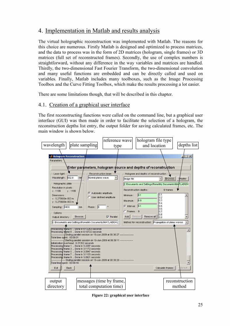
4.1. Creation of a graphical user interface
The first reconstructing functions were called on the command line, but a graphical user
interface (GUI) was then made in order to facilitate the selection of a hologram, the
reconstruction depths list entry, the output folder for saving calculated frames, etc. The
main window is shown below.
Figure 22: graphical user interface
wavelength plate sampling reference wave
type
hologram file type
and location
output
directory
depths list
messages (time by frame,
total computation time)
reconstruction
method
26
The goal of creating a GUI is to enable an easy use of the software with a user-friendly
interface, and to broaden its use to other cases. For example, the holographic plate
resolution in pixels and the sampling value are not fixed, and a different camera can be
used; a different wavelength can be entered if a different laser is used… The GUI calls
one of the reconstruction functions when the “Calculate frames” button is clicked, and
the “Result” button is activated once the calculation is complete. Pressing this latter
launches the calculation of the intensity (Appendix 5) on the optical fields previously
calculated, and displays the different depths using the Matlab function “implay”, which
is a frame-by-frame viewer.
The GUI was developed at first using “guide”, a Matlab graphical environment for
designing GUIs. This tool saves two different files: a “.fig” file which represents the
figure with the locations of the different controls, listboxes and buttons, and a “.m” file
(m-file) including the code for the initialization of the GUI and the actions performed
when a value is entered, a button is clicked or a listbox value is selected. Although
creating a GUI is easier when using this tool, some restrictions on the way variables are
handled within the GUI exist. Also, “guide” crashed after many hours of work on the
GUI, and the corresponding “.fig” file was corrupted. After some research on the
Mathworks website, it appeared that this was a known bug in Matlab 2008a, and that
nothing could be done to recover the file. For these reasons, the choice was made to
write the GUI programmatically, in a self-contained m-file. Even if defining all the
parameters for each control is a bit cumbersome, this has several advantages, in
particular to locate precisely the controls, to be able to have a custom system of
variables handling and sharing with the functions called, and to be able to recover from
a bug (Matlab automatically saves a back-up of m-files when changes are made).
The full code of the GUI can be found with the indications in Appendix 5. Some
functions were added to check values and paths entered in the fields, enable the
calculation only if all the required parameters have been entered, and make the
propagation calculation either in serial mode or in parallel.
4.2. Reconstruction functions
4.2.1. Convolution method
The first reconstruction function to be implemented is the decomposition in spherical
waves, named “Convolution (Fresnel pattern)” in the program because it makes the
convolution between the hologram and a Fresnel zone plate pattern (in fact, the real part
of the field is a zone plate pattern, but the convolution is calculated with the complex
field). It was programmed at first as a ray-tracing method, basically calculating the field
of a point of the hologram at the reconstructed plane depending on the optical paths, and
adding all the fields to find the final propagated field. The code was then changed to use
the “conv2” function in Matlab to take advantage of the fact that this operation is a two-
dimensional convolution between the hologram and the field from a point source at the
distance d (distance between the hologram and the reconstructed plane). Doing so, it is
enough to calculate once the field, and to apply the “conv2” function. This enables to
simplify the code and to speed up the calculation. Still it is much slower that the final
implementation, using the Fourier transform to calculate the convolution thanks to the
convolution theorem. As an example, here are some computation times for a 1024 x
1024 pixels hologram on a Pentium M 1.75GHz: (see next page)
27
- conv2: 130.7 s
- Fourier: 3.6 s
This big difference of calculation time is due to the big difference in the number of
operations to perform: for one point of the reconstructed plane, the “conv2” function
performs N1xN2 multiplications and N1xN2 additions. This must be done for all the
reconstructed plane points, N1xN2 times (N1 and N2 being the number of pixels in x and
y).
In contrast, the fast Fourier transform takes [ ] [ ]1 1 2 2 2 12 ln( ) 2 ln( )N N N N N N× + ×
operations (rows and columns). There are two FFT calls in the Fourier transform
implementation, and the product between the two fields takes N1xN2 multiplications. N1
and N2 are powers of 2 to ensure that the FFT algorithm runs at its optimized speed (this
is done by zero-padding the matrices up to the next power of 2).
As a summary, the “conv2” function takes about 2 2
1 22N N operations, and the Fourier
transform implementation takes ( ) ( )1 2 1 2 1 24 ln lnN N N N N N+ + operations. Of course
Matlab performs other operations to convert the complex fields from Cartesian form to
polar form and back when calculating multiplications, and N1 and N2 may not be the
same between the two methods due to the power of 2 length in the second one. However
this is given as an approximation, to show that the difference comes from the square
factor for the “conv2” method.
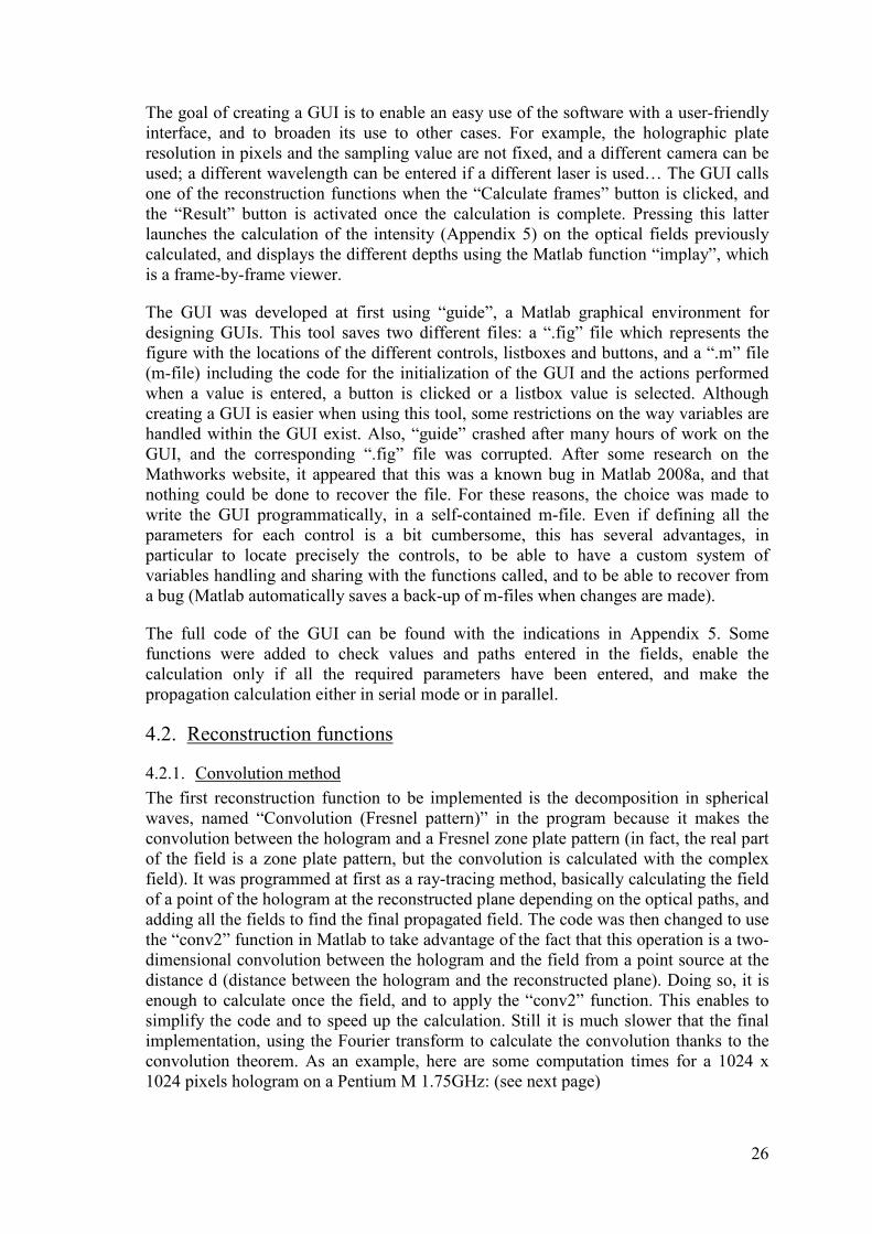
The final code (Appendix 5) includes a faster method to calculate the field from a point
source at the distance d: instead of calculating the field pointwise for every point, only
one row and one column are calculated. These are the columns at the center of the field,
where either ' 0x x− = or 'y y− =0. Then the full matrix is obtained by performing a
matrix product between the column vector and the row vector. The two methods are
equivalent only if the Fresnel approximation at the first order is used:
( ) ( ) ( ) ( )2 2 2
2 2
2 2
' ' '' 1 1
2 2
x x x x x xr x x d d d d
d d d
− − −= − + = + = + = +
21)
Additionally, only one quarter of the field is calculated and replicated using horizontal
and vertical symmetries.
matrix product:
column vector
x
row vector
horizontal
symmetry
vertical
symmetry
Figure 23: efficient way of calculating the field from a point source on a plane (real part displayed)
28
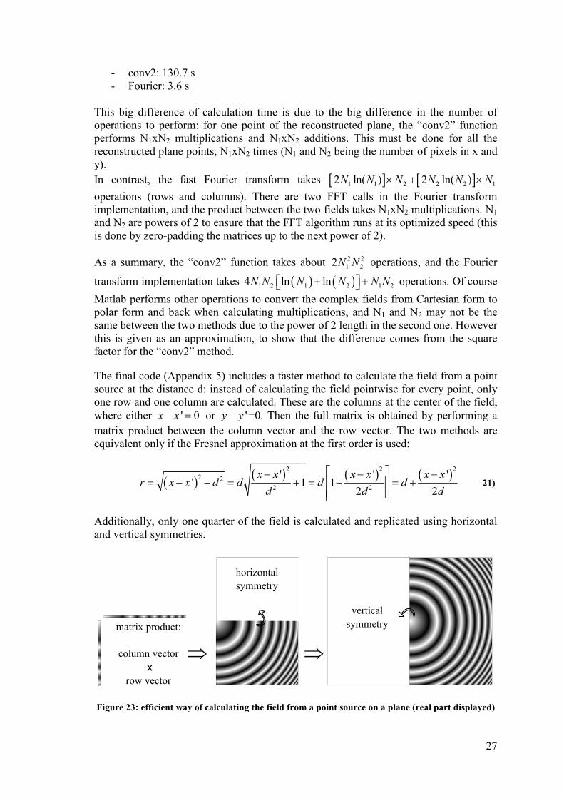
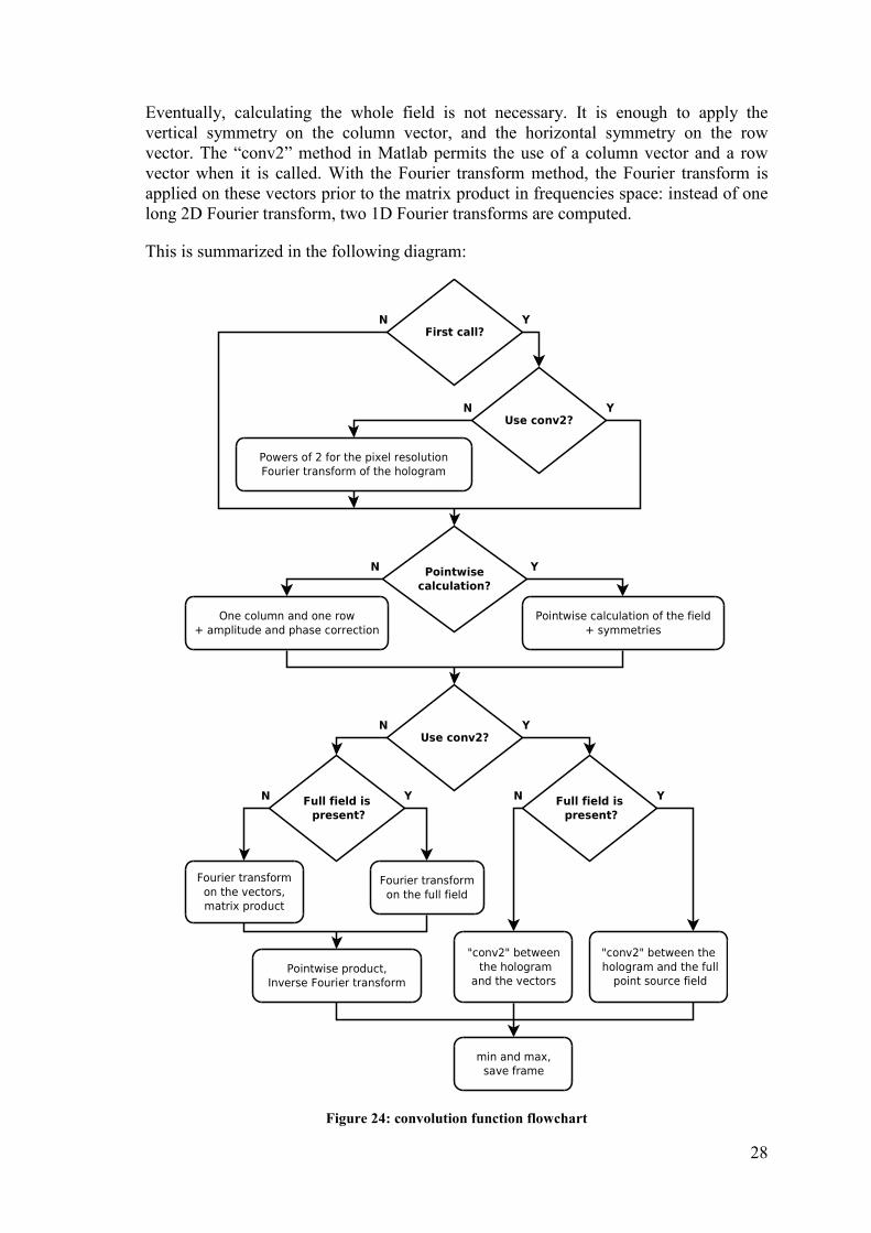
Eventually, calculating the whole field is not necessary. It is enough to apply the
vertical symmetry on the column vector, and the horizontal symmetry on the row
vector. The “conv2” method in Matlab permits the use of a column vector and a row
vector when it is called. With the Fourier transform method, the Fourier transform is
applied on these vectors prior to the matrix product in frequencies space: instead of one
long 2D Fourier transform, two 1D Fourier transforms are computed.
This is summarized in the following diagram:
First call?Y
Powers of 2 for the pixel resolution
Fourier transform of the hologram
Use conv2?N Y
N
Pointwise
calculation?
Y
Pointwise calculation of the field
+ symmetries
N
One column and one row
+ amplitude and phase correction
Use conv2?YN
Full field is
present?
Full field is
present?
YYN N
"conv2" between the
hologram and the full
point source field
"conv2" between
the hologram
and the vectors
Fourier transform
on the vectors,
matrix product
Fourier transform
on the full field
Pointwise product,
Inverse Fourier transform
min and max,
save frame
Figure 24: convolution function flowchart
29
Parameters for the reconstruction such as the hologram, the depths list and the spatial
coordinates are accessed by the convolution function through the use of a global
variable. The frame number is passed to the function as an argument, to indicate which
depth to use in the depth list for the current iteration. The Fourier transform of the
hologram is calculated only once, for the first call of the function. It is not calculated
again for subsequent calls in case of several depths to process. This is achieved with the
use of a persistent variable.
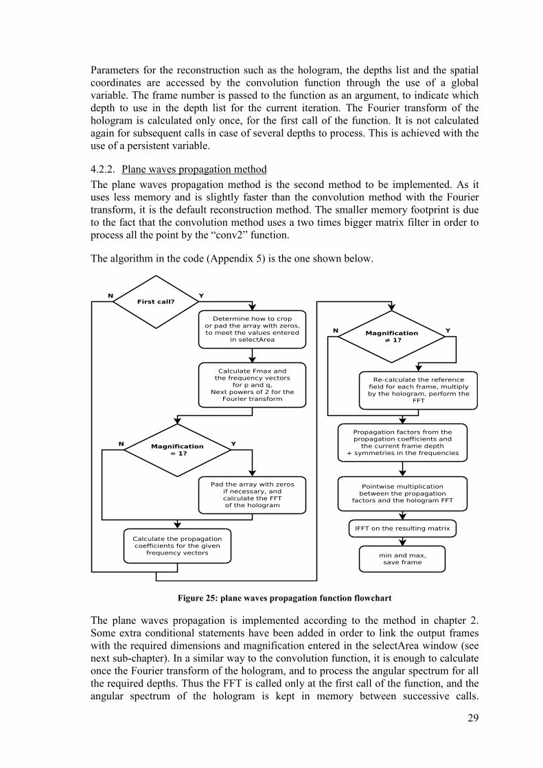
4.2.2. Plane waves propagation method
The plane waves propagation method is the second method to be implemented. As it
uses less memory and is slightly faster than the convolution method with the Fourier
transform, it is the default reconstruction method. The smaller memory footprint is due
to the fact that the convolution method uses a two times bigger matrix filter in order to
process all the point by the “conv2” function.
The algorithm in the code (Appendix 5) is the one shown below.
Calculate Fmax and
the frequency vectors
for p and q,
Next powers of 2 for the
Fourier transform
First call?YN
Magnification
= 1?
YN
Pad the array with zeros
if necessary, and
calculate the FFT
of the hologram
Determine how to crop
or pad the array with zeros,
to meet the values entered
in selectArea
Calculate the propagation
coefficients for the given
frequency vectors
Magnification
≠ 1?
YN
Re-calculate the reference
field for each frame, multiply
by the hologram, perform the
FFT
Propagation factors from the
propagation coefficients and
the current frame depth
+ symmetries in the frequencies
Pointwise multiplication
between the propagation
factors and the hologram FFT
IFFT on the resulting matrix
min and max,
save frame
Figure 25: plane waves propagation function flowchart
The plane waves propagation is implemented according to the method in chapter 2.
Some extra conditional statements have been added in order to link the output frames
with the required dimensions and magnification entered in the selectArea window (see
next sub-chapter). In a similar way to the convolution function, it is enough to calculate
once the Fourier transform of the hologram, and to process the angular spectrum for all
the required depths. Thus the FFT is called only at the first call of the function, and the
angular spectrum of the hologram is kept in memory between successive calls.
30
However, with the introduction of a magnification factor, a different reference field is
used for each reconstruction depth, and the field emerging from the hologram is
different for every iteration. In this case, the FFT must be computed for every call. This
is the reason for the existence of a magnification factor condition in the “First call” part
of the function, and in the main part.
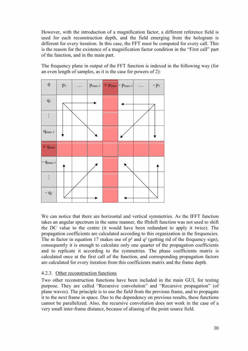
The frequency plane in output of the FFT function is indexed in the following way (for
an even length of samples, as it is the case for powers of 2):
0 p1 … pmax-1 ± pmax - pmax-1 … - p1
q1
⋮
qmax-1
± qmax
- qmax-1
⋮
- q1
We can notice that there are horizontal and vertical symmetries. As the IFFT function
takes an angular spectrum in the same manner, the fftshift function was not used to shift
the DC value to the centre (it would have been redundant to apply it twice). The
propagation coefficients are calculated according to this organization in the frequencies.
The m factor in equation 17 makes use of p² and q² (getting rid of the frequency sign),
consequently it is enough to calculate only one quarter of the propagation coefficients
and to replicate it according to the symmetries. The phase coefficients matrix is
calculated once at the first call of the function, and corresponding propagation factors
are calculated for every iteration from this coefficients matrix and the frame depth.
4.2.3. Other reconstruction functions
Two other reconstruction functions have been included in the main GUI, for testing
purpose. They are called “Recursive convolution” and “Recursive propagation” (of
plane waves). The principle is to use the field from the previous frame, and to propagate
it to the next frame in space. Due to the dependency on previous results, these functions
cannot be parallelized. Also, the recursive convolution does not work in the case of a
very small inter-frame distance, because of aliasing of the point source field.
31
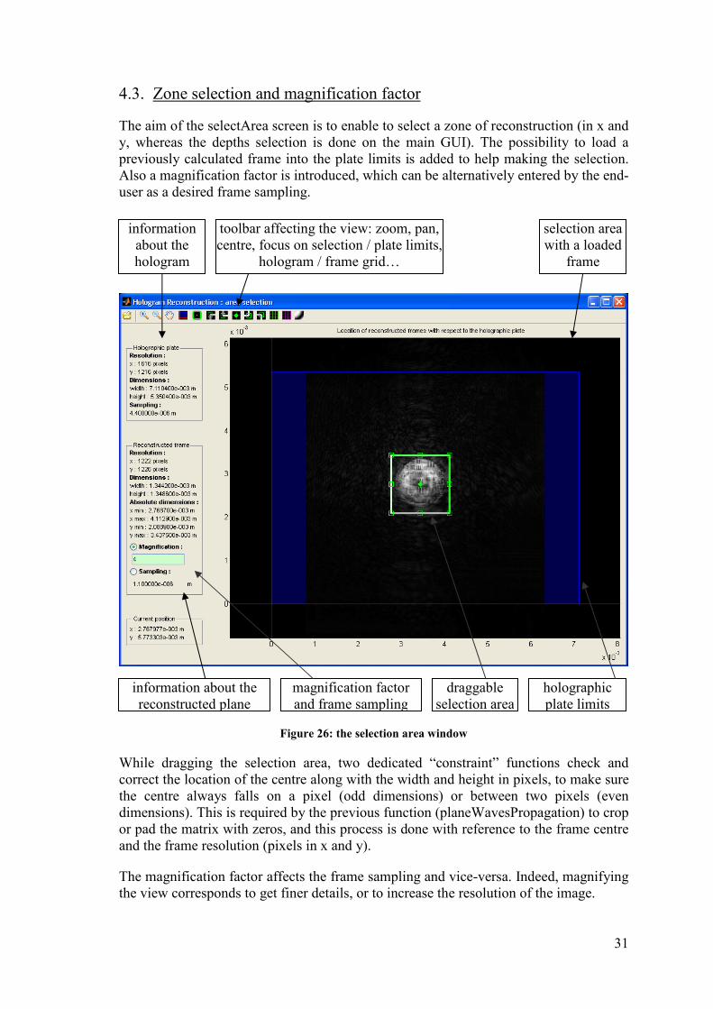
4.3. Zone selection and magnification factor
The aim of the selectArea screen is to enable to select a zone of reconstruction (in x and
y, whereas the depths selection is done on the main GUI). The possibility to load a
previously calculated frame into the plate limits is added to help making the selection.
Also a magnification factor is introduced, which can be alternatively entered by the end-
user as a desired frame sampling.
Figure 26: the selection area window
While dragging the selection area, two dedicated “constraint” functions check and
correct the location of the centre along with the width and height in pixels, to make sure
the centre always falls on a pixel (odd dimensions) or between two pixels (even
dimensions). This is required by the previous function (planeWavesPropagation) to crop
or pad the matrix with zeros, and this process is done with reference to the frame centre
and the frame resolution (pixels in x and y).
The magnification factor affects the frame sampling and vice-versa. Indeed, magnifying
the view corresponds to get finer details, or to increase the resolution of the image.
information
about the
hologram
toolbar affecting the view: zoom, pan,
centre, focus on selection / plate limits,
hologram / frame grid…
selection area
with a loaded
frame
information about the
reconstructed plane
magnification factor
and frame sampling
draggable
selection area
holographic
plate limits

32
The code for selectArea is available on the CD, see Appendix 5.
4.4. Computing resources compromises
The first problem that arose from the very beginning is the memory footprint. Indeed
processing complex optical fields in variable type “double” (Matlab default for high
precision) and with powers of 2 lengths for the Fourier transform takes a lot of memory.
Basically, it is not possible to keep all the calculated frames in memory as separate
variables, because the limits of the physical memory are reached even for a small
number of calculated depths. There is also a limit to the maximum array size, because
variables are created in contiguous blocks of memory. As an example, a complex array
of 2048 x 2048 values takes ( )22048 2048 8 2 / 1024 64 MB× × × = . One solution to
reduce this amount is to use “single” type instead of “double”, which takes two times
less memory at the cost of precision. However Matlab operations and functions are
processed in “double” by default, and the variables will be reconverted to “double” if
not specified otherwise.
On top of this must be added the system memory, the Matlab program size in RAM
(about 163 MB) and the fact that several big arrays are involved when the
reconstruction methods are applied. Also, when a function is called in Matlab, variables
are not shared but copied instead, leading to additional transient peaks of memory use.
For these reasons, it was decided to save each reconstructed field in a file on the hard
drive, before calculating the next one. Doing so, the memory usage is kept below hitting
the “virtual memory” (the use of the memory swap file must be avoided, since the
computation becomes much slower when the operating system is competing with
Matlab to read and write on the physical drive). The computer used at the laboratory
had 2GB of installed RAM, which was enough most of the time.
The second concern is about computation speed. Matlab is a single threaded application
therefore functions running in parallel are not permitted. By enabling the
“multithreading computations” in the preferences, some elementwise functions such as
sin and log can take profit of a multicore processor, however it does not allow parallel
functions.
The computer available at the laboratory is fit with a powerful Quad-core processor, the
Intel E6600 (2.4GHz). A single frame does not take much time to compute (2.8s in
average with the plane waves propagation method), still it is not used at its maximum
potential. Only one quarter of the processor is working at a time. Propagation to
different depths could be performed in parallel though, since each iteration is
independent of the other ones. Hence different parallelization schemes have been
assessed.
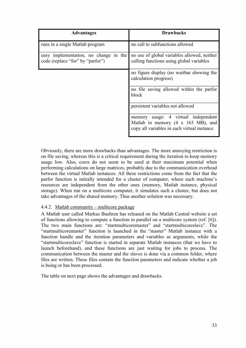
4.4.1. The parfor function
The Parallel Computing Toolbox includes a function called parfor. It is typically a “for”
loop, executing a given number of iterations, but these iterations are randomly
distributed to the participating computers present in the Matlab pool. The following
table summarizes its advantages and its drawbacks.
33
Advantages Drawbacks
runs in a single Matlab program no call to subfunctions allowed
easy implementation, no change in the
code (replace “for” by “parfor”)
no use of global variables allowed, neither
calling functions using global variables
no figure display (no waitbar showing the
calculation progress)
no file saving allowed within the parfor
block
persistent variables not allowed
memory usage: 4 virtual independent
Matlab in memory (4 x 163 MB), and
copy all variables in each virtual instance
Obviously, there are more drawbacks than advantages. The more annoying restriction is
on file saving, whereas this is a critical requirement during the iteration to keep memory
usage low. Also, cores do not seem to be used at their maximum potential when
performing calculations on large matrices, probably due to the communication overhead
between the virtual Matlab instances. All these restrictions come from the fact that the
parfor function is initially intended for a cluster of computer, where each machine’s
resources are independent from the other ones (memory, Matlab instance, physical
storage). When run on a multicore computer, it simulates such a cluster, but does not
take advantages of the shared memory. Thus another solution was necessary.
4.4.2. Matlab community – multicore package
A Matlab user called Markus Buehren has released on the Matlab Central website a set
of functions allowing to compute a function in parallel on a multicore system (ref. [6]).
The two main functions are: “startmulticoremaster” and “startmulticoreslave”. The
“startmulticoremaster” function is launched in the “master” Matlab instance with a
function handle and the iteration parameters and variables as arguments, while the
“startmulticoreslave” function is started in separate Matlab instances (that we have to
launch beforehand), and these functions are just waiting for jobs to process. The
communication between the master and the slaves is done via a common folder, where
files are written. These files contain the function parameters and indicate whether a job
is being or has been processed.
The table on next page shows the advantages and drawbacks.
34
Advantages Drawbacks
save frames in files for each iteration file system overhead (read and write the
variables on the hard drive)
straightforward adaptation from a
multicore computer to a cluster of
computers (it is enough to have a shared
directory)
does not make the difference between
fixed parameters (the hologram) and
variable parameters (list of depths) – all
parameters are transferred for every
iteration
add slaves dynamically during the process 4 Matlab instances must be launched on
the same computer (4 x 163 MB)
use a waitbar to show the progress the provided waitbar is not reliable
The trade-offs are more balanced in the case of this alternative, nevertheless the fact that
all parameters are read again for each iteration limits the efficiency, and the waitbar is
very annoying (it does not give a right clue of the actual progress state).
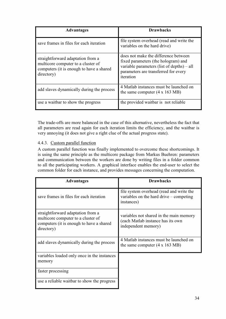
4.4.3. Custom parallel function
A custom parallel function was finally implemented to overcome these shortcomings. It
is using the same principle as the multicore package from Markus Buehren: parameters
and communication between the workers are done by writing files in a folder common
to all the participating workers. A graphical interface enables the end-user to select the
common folder for each instance, and provides messages concerning the computation.
Advantages Drawbacks
save frames in files for each iteration
file system overhead (read and write the
variables on the hard drive – competing
instances)
straightforward adaptation from a
multicore computer to a cluster of
computers (it is enough to have a shared
directory)
variables not shared in the main memory
(each Matlab instance has its own
independent memory)
add slaves dynamically during the process 4 Matlab instances must be launched on
the same computer (4 x 163 MB)
variables loaded only once in the instances
memory
faster processing
use a reliable waitbar to show the progress
35
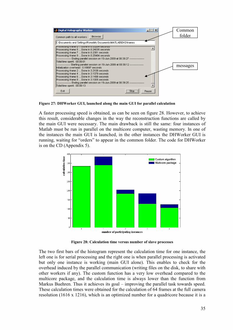
Figure 27: DHWorker GUI, launched along the main GUI for parallel calculation
A faster processing speed is obtained, as can be seen on figure 28. However, to achieve
this result, considerable changes in the way the reconstruction functions are called by
the main GUI were necessary. The main drawback is still the same: four instances of
Matlab must be run in parallel on the multicore computer, wasting memory. In one of
the instances the main GUI is launched, in the other instances the DHWorker GUI is
running, waiting for “orders” to appear in the common folder. The code for DHWorker
is on the CD (Appendix 5).
Figure 28: Calculation time versus number of slave processes
The two first bars of the histogram represent the calculation time for one instance, the
left one is for serial processing and the right one is when parallel processing is activated
but only one instance is working (main GUI alone). This enables to check for the
overhead induced by the parallel communication (writing files on the disk, to share with
other workers if any). The custom function has a very low overhead compared to the
multicore package, and the calculation time is always lower than the function from
Markus Buehren. Thus it achieves its goal – improving the parallel task towards speed.
These calculation times were obtained for the calculation of 64 frames at the full camera
resolution (1616 x 1216), which is an optimized number for a quadricore because it is a
Common
folder
messages
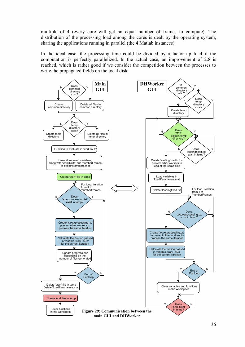
36
multiple of 4 (every core will get an equal number of frames to compute). The
distribution of the processing load among the cores is dealt by the operating system,
sharing the applications running in parallel (the 4 Matlab instances).
In the ideal case, the processing time could be divided by a factor up to 4 if the
computation is perfectly parallelized. In the actual case, an improvement of 2.8 is
reached, which is rather good if we consider the competition between the processes to
write the propagated fields on the local disk.
Doescommon directory
exist?
Y
Doestemp
directoryexist?
Create tempdirectory
N Y
Does'xxxxxprocessing.txt'
exist in temp?
Y
Create ‘xxxxxprocessing’ toprevent other workers to
process the same iteration
Calculate the funtion passedin variable 'workToDo'for the current iteration
For loop, iterationfrom 1 to'numberFrames'
Clear functionsin the workspace
End ofFor loop
N
NY
Delete all files incommon directory
Createcommon directory
N
Delete all files intemp directory
Function to evaluate in 'workToDo'
Save all required variables,along with 'workToDo' and 'numberFrames',
in 'fixedParameters.mat'
Create 'start' file in temp
Update progress bardepending on the
number of files generated
Create 'end' file in temp
Delete 'start' file in tempDelete 'fixedParameters.mat'
Iscommon directory
valid?
Y
Doestemp
directoryexist?
Create tempdirectory
N
Does‘start’
exist in tempdirectory?
Y
Does‘loadingfixed.txt’exist in temp?
N Y
Create ‘loadingfixed.txt’ toprevent other workers to
load at the same time
Load variables in‘fixedParameters.mat’
Delete ‘loadingfixed.txt’
N Y
Does'xxxxxprocessing.txt'
exist in temp?
Y
Create ‘xxxxxprocessing.txt’to prevent other workers toprocess the same iteration
Calculate the funtion passedin variable 'workToDo'for the current iteration
For loop, iterationfrom 1 to'numberFrames'
Clear variables and functionsin the workspace
End ofFor loop
N
NY
Does‘end’ existin temp?
NY
Figure 29: Communication between the
main GUI and DHWorker
Main
GUI
DHWorker
GUI
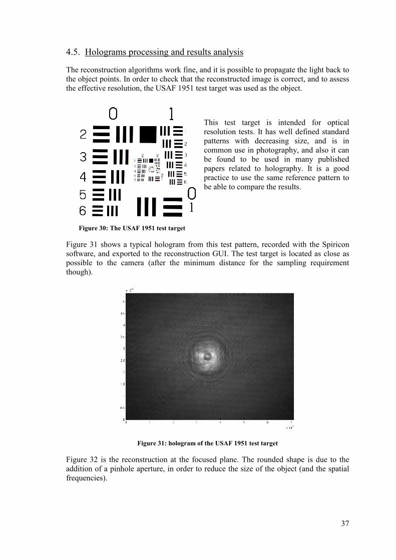
37
4.5. Holograms processing and results analysis
The reconstruction algorithms work fine, and it is possible to propagate the light back to
the object points. In order to check that the reconstructed image is correct, and to assess
the effective resolution, the USAF 1951 test target was used as the object.
This test target is intended for optical
resolution tests. It has well defined standard
patterns with decreasing size, and is in
common use in photography, and also it can
be found to be used in many published
papers related to holography. It is a good
practice to use the same reference pattern to
be able to compare the results.
Figure 30: The USAF 1951 test target
Figure 31 shows a typical hologram from this test pattern, recorded with the Spiricon
software, and exported to the reconstruction GUI. The test target is located as close as
possible to the camera (after the minimum distance for the sampling requirement
though).
Figure 31: hologram of the USAF 1951 test target
Figure 32 is the reconstruction at the focused plane. The rounded shape is due to the
addition of a pinhole aperture, in order to reduce the size of the object (and the spatial
frequencies).
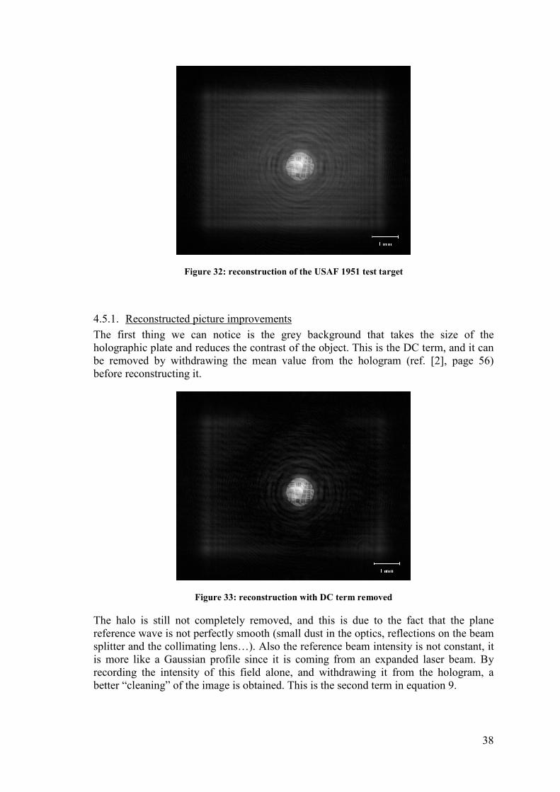
38
Figure 32: reconstruction of the USAF 1951 test target
4.5.1. Reconstructed picture improvements
The first thing we can notice is the grey background that takes the size of the
holographic plate and reduces the contrast of the object. This is the DC term, and it can
be removed by withdrawing the mean value from the hologram (ref. [2], page 56)
before reconstructing it.
Figure 33: reconstruction with DC term removed
The halo is still not completely removed, and this is due to the fact that the plane
reference wave is not perfectly smooth (small dust in the optics, reflections on the beam
splitter and the collimating lens…). Also the reference beam intensity is not constant, it
is more like a Gaussian profile since it is coming from an expanded laser beam. By
recording the intensity of this field alone, and withdrawing it from the hologram, a
better “cleaning” of the image is obtained. This is the second term in equation 9.
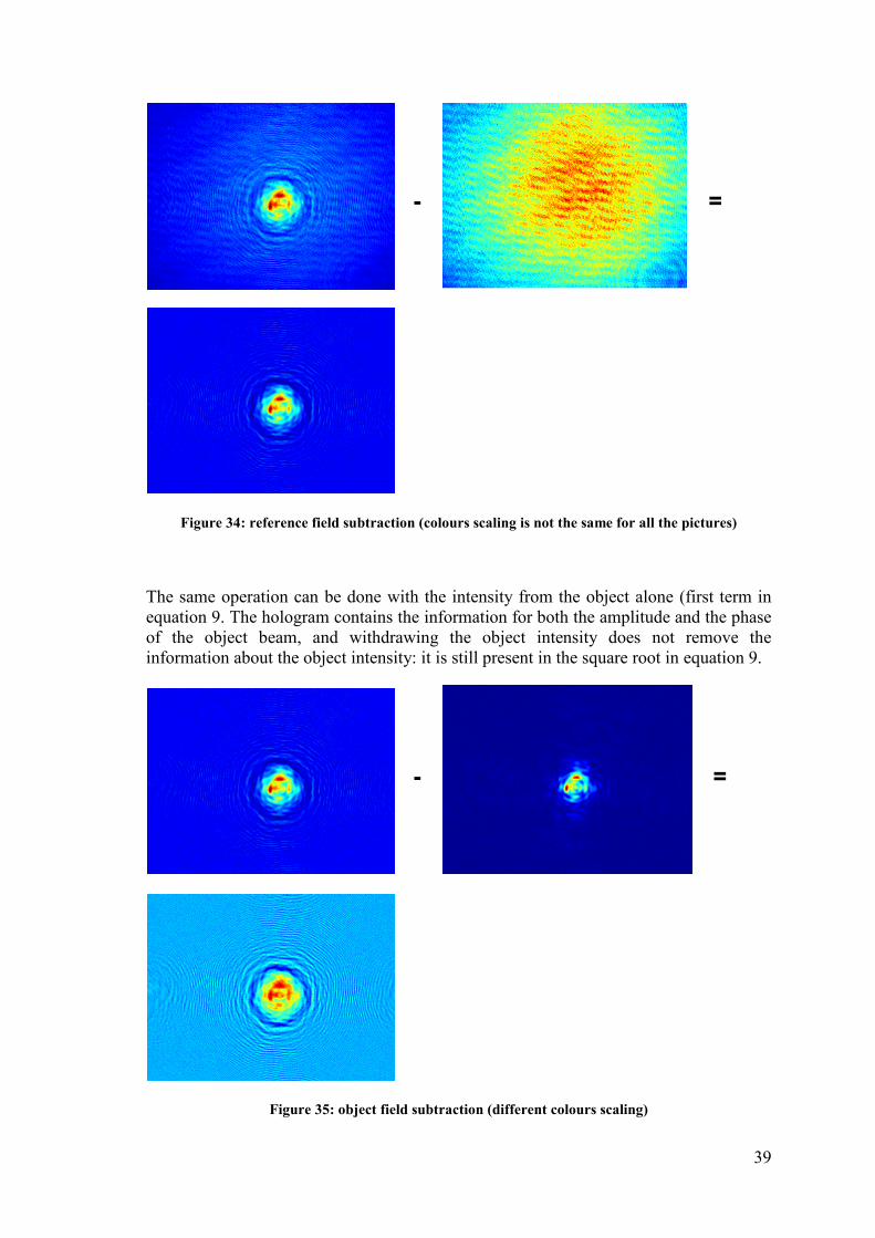
39
Figure 34: reference field subtraction (colours scaling is not the same for all the pictures)
The same operation can be done with the intensity from the object alone (first term in
equation 9. The hologram contains the information for both the amplitude and the phase
of the object beam, and withdrawing the object intensity does not remove the
information about the object intensity: it is still present in the square root in equation 9.
Figure 35: object field subtraction (different colours scaling)
- =
- =
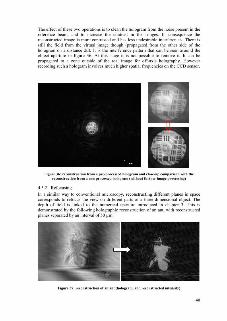
40
The effect of these two operations is to clean the hologram from the noise present in the
reference beam, and to increase the contrast in the fringes. In consequence the
reconstructed image is more contrasted and has less undesirable interferences. There is
still the field from the virtual image though (propagated from the other side of the
hologram on a distance 2d). It is the interference pattern that can be seen around the
object aperture in figure 36. At this stage it is not possible to remove it. It can be
propagated to a zone outside of the real image for off-axis holography. However
recording such a hologram involves much higher spatial frequencies on the CCD sensor.
Figure 36: reconstruction from a pre-processed hologram and close-up comparison with the
reconstruction from a non processed hologram (without further image processing)
4.5.2. Refocusing
In a similar way to conventional microscopy, reconstructing different planes in space
corresponds to refocus the view on different parts of a three-dimensional object. The
depth of field is linked to the numerical aperture introduced in chapter 3. This is
demonstrated by the following holographic reconstruction of an ant, with reconstructed
planes separated by an interval of 50 µm:
Figure 37: reconstruction of an ant (hologram, and reconstructed intensity)
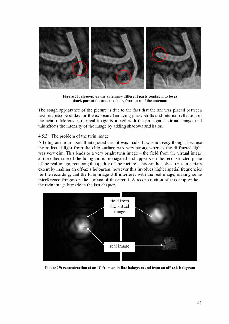
41
Figure 38: close-up on the antenna – different parts coming into focus
(back part of the antenna, hair, front part of the antenna)
The rough appearance of the picture is due to the fact that the ant was placed between
two microscope slides for the exposure (inducing phase shifts and internal reflection of
the beam). Moreover, the real image is mixed with the propagated virtual image, and
this affects the intensity of the image by adding shadows and halos.
4.5.3. The problem of the twin image
A hologram from a small integrated circuit was made. It was not easy though, because
the reflected light from the chip surface was very strong whereas the diffracted light
was very dim. This leads to a very bright twin image – the field from the virtual image
at the other side of the hologram is propagated and appears on the reconstructed plane
of the real image, reducing the quality of the picture. This can be solved up to a certain
extent by making an off-axis hologram, however this involves higher spatial frequencies
for the recording, and the twin image still interferes with the real image, making some
interference fringes on the surface of the circuit. A reconstruction of this chip without
the twin image is made in the last chapter.
Figure 39: reconstruction of an IC from an in-line hologram and from an off-axis hologram
real image
field from
the virtual
image
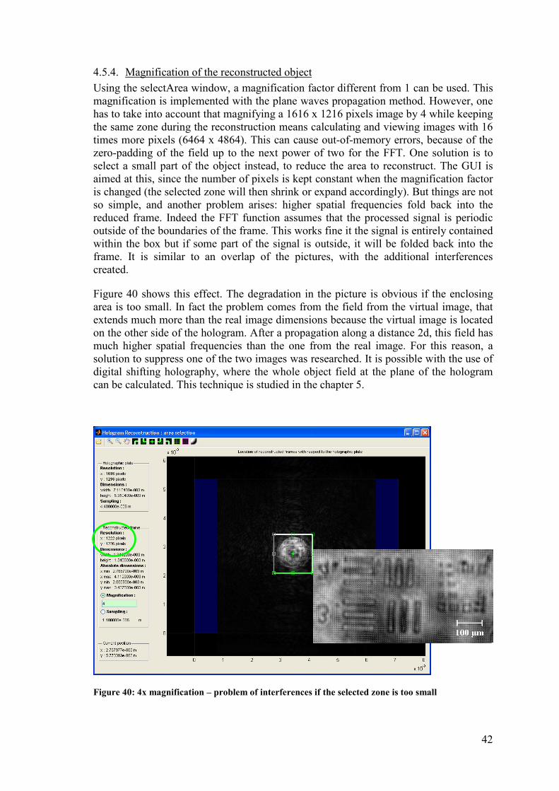
42
4.5.4. Magnification of the reconstructed object
Using the selectArea window, a magnification factor different from 1 can be used. This
magnification is implemented with the plane waves propagation method. However, one
has to take into account that magnifying a 1616 x 1216 pixels image by 4 while keeping
the same zone during the reconstruction means calculating and viewing images with 16
times more pixels (6464 x 4864). This can cause out-of-memory errors, because of the
zero-padding of the field up to the next power of two for the FFT. One solution is to
select a small part of the object instead, to reduce the area to reconstruct. The GUI is
aimed at this, since the number of pixels is kept constant when the magnification factor
is changed (the selected zone will then shrink or expand accordingly). But things are not
so simple, and another problem arises: higher spatial frequencies fold back into the
reduced frame. Indeed the FFT function assumes that the processed signal is periodic
outside of the boundaries of the frame. This works fine it the signal is entirely contained
within the box but if some part of the signal is outside, it will be folded back into the
frame. It is similar to an overlap of the pictures, with the additional interferences
created.
Figure 40 shows this effect. The degradation in the picture is obvious if the enclosing
area is too small. In fact the problem comes from the field from the virtual image, that
extends much more than the real image dimensions because the virtual image is located
on the other side of the hologram. After a propagation along a distance 2d, this field has
much higher spatial frequencies than the one from the real image. For this reason, a
solution to suppress one of the two images was researched. It is possible with the use of
digital shifting holography, where the whole object field at the plane of the hologram
can be calculated. This technique is studied in the chapter 5.
Figure 40: 4x magnification – problem of interferences if the selected zone is too small
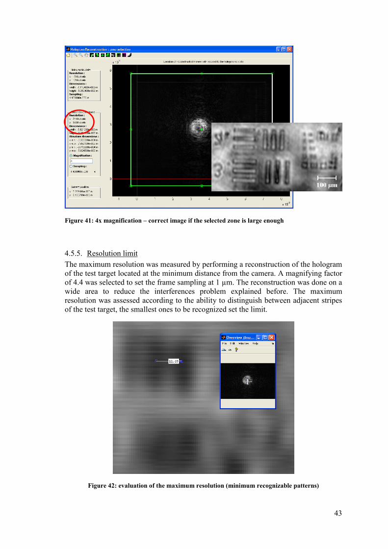
43
Figure 41: 4x magnification – correct image if the selected zone is large enough
4.5.5. Resolution limit
The maximum resolution was measured by performing a reconstruction of the hologram
of the test target located at the minimum distance from the camera. A magnifying factor
of 4.4 was selected to set the frame sampling at 1 µm. The reconstruction was done on a
wide area to reduce the interferences problem explained before. The maximum
resolution was assessed according to the ability to distinguish between adjacent stripes
of the test target, the smallest ones to be recognized set the limit.
Figure 42: evaluation of the maximum resolution (minimum recognizable patterns)
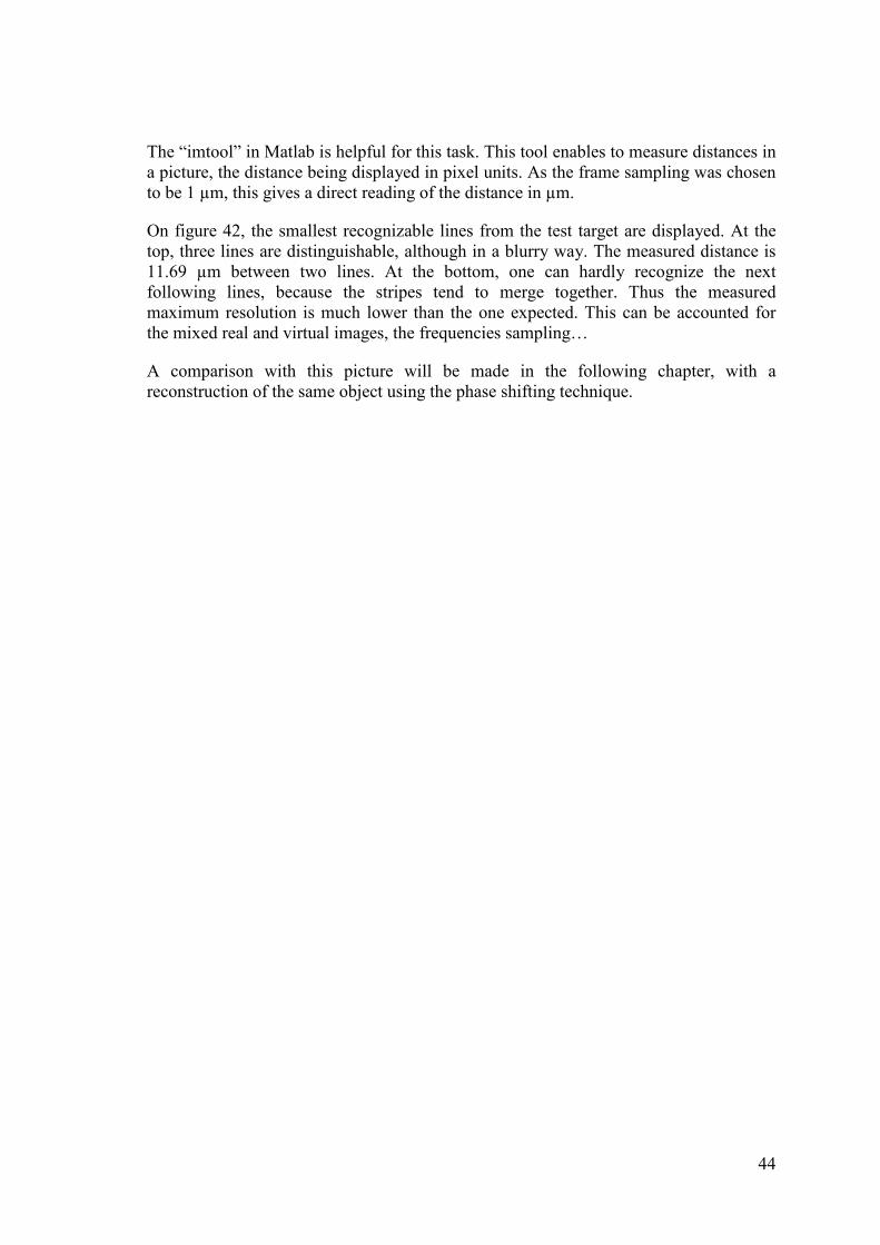
44
The “imtool” in Matlab is helpful for this task. This tool enables to measure distances in
a picture, the distance being displayed in pixel units. As the frame sampling was chosen
to be 1 µm, this gives a direct reading of the distance in µm.
On figure 42, the smallest recognizable lines from the test target are displayed. At the
top, three lines are distinguishable, although in a blurry way. The measured distance is
11.69 µm between two lines. At the bottom, one can hardly recognize the next
following lines, because the stripes tend to merge together. Thus the measured
maximum resolution is much lower than the one expected. This can be accounted for
the mixed real and virtual images, the frequencies sampling…
A comparison with this picture will be made in the following chapter, with a
reconstruction of the same object using the phase shifting technique.
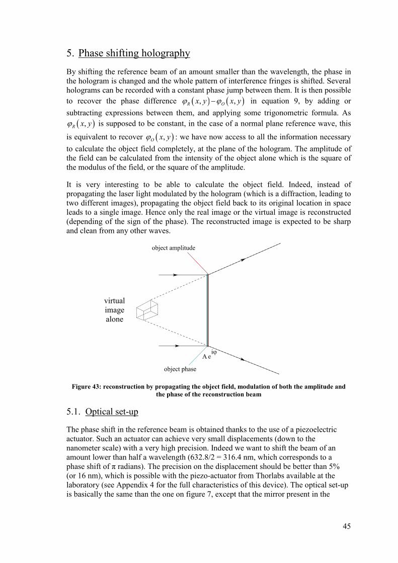
45
5. Phase shifting holography
By shifting the reference beam of an amount smaller than the wavelength, the phase in
the hologram is changed and the whole pattern of interference fringes is shifted. Several
holograms can be recorded with a constant phase jump between them. It is then possible
to recover the phase difference ( ) ( ), ,R Ox y x yϕ ϕ− in equation 9, by adding or
subtracting expressions between them, and applying some trigonometric formula. As
( ),R x yϕ is supposed to be constant, in the case of a normal plane reference wave, this
is equivalent to recover ( ),O x yϕ : we have now access to all the information necessary
to calculate the object field completely, at the plane of the hologram. The amplitude of
the field can be calculated from the intensity of the object alone which is the square of
the modulus of the field, or the square of the amplitude.
It is very interesting to be able to calculate the object field. Indeed, instead of
propagating the laser light modulated by the hologram (which is a diffraction, leading to
two different images), propagating the object field back to its original location in space
leads to a single image. Hence only the real image or the virtual image is reconstructed
(depending of the sign of the phase). The reconstructed image is expected to be sharp
and clean from any other waves.
Figure 43: reconstruction by propagating the object field, modulation of both the amplitude and
the phase of the reconstruction beam
5.1. Optical set-up
The phase shift in the reference beam is obtained thanks to the use of a piezoelectric
actuator. Such an actuator can achieve very small displacements (down to the
nanometer scale) with a very high precision. Indeed we want to shift the beam of an
amount lower than half a wavelength (632.8/2 = 316.4 nm, which corresponds to a
phase shift of π radians). The precision on the displacement should be better than 5%
(or 16 nm), which is possible with the piezo-actuator from Thorlabs available at the
laboratory (see Appendix 4 for the full characteristics of this device). The optical set-up
is basically the same than the one on figure 7, except that the mirror present in the
virtual
image
alone
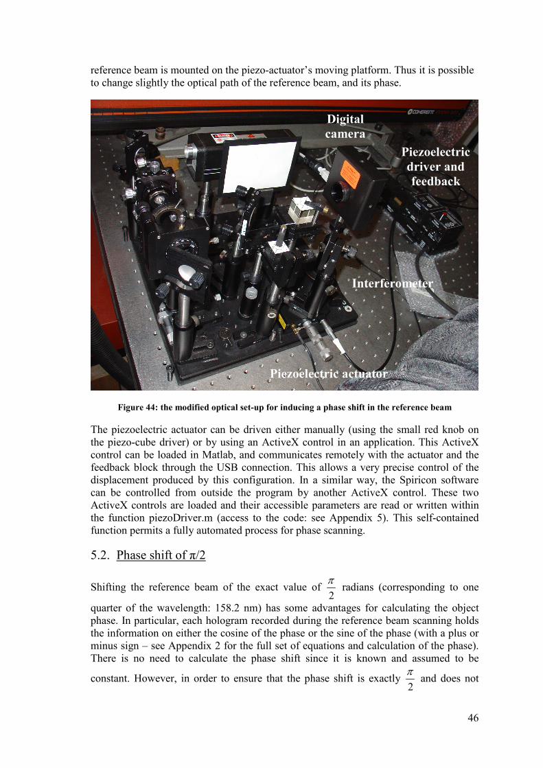
46
reference beam is mounted on the piezo-actuator’s moving platform. Thus it is possible
to change slightly the optical path of the reference beam, and its phase.
Figure 44: the modified optical set-up for inducing a phase shift in the reference beam
The piezoelectric actuator can be driven either manually (using the small red knob on
the piezo-cube driver) or by using an ActiveX control in an application. This ActiveX
control can be loaded in Matlab, and communicates remotely with the actuator and the
feedback block through the USB connection. This allows a very precise control of the
displacement produced by this configuration. In a similar way, the Spiricon software
can be controlled from outside the program by another ActiveX control. These two
ActiveX controls are loaded and their accessible parameters are read or written within
the function piezoDriver.m (access to the code: see Appendix 5). This self-contained
function permits a fully automated process for phase scanning.
5.2. Phase shift of π/2
Shifting the reference beam of the exact value of 2
π radians (corresponding to one
quarter of the wavelength: 158.2 nm) has some advantages for calculating the object
phase. In particular, each hologram recorded during the reference beam scanning holds
the information on either the cosine of the phase or the sine of the phase (with a plus or
minus sign – see Appendix 2 for the full set of equations and calculation of the phase).
There is no need to calculate the phase shift since it is known and assumed to be
constant. However, in order to ensure that the phase shift is exactly 2
π and does not
Digital
camera
Piezoelectric
driver and
feedback
Interferometer
Piezoelectric actuator
47
vary through the scanning process, additional effort is necessary to calibrate the
actuator. The calibration procedure that was used is explained in Appendix 3. Some
experiments were performed with success by using this method. Nevertheless, the
calibration procedure is very long and must be very precise, and it needs to be done
again between different phase scanning sessions because the voltage value required to
shift the piezo-actuator of the precise value of 2
π seems to change through time,
depending on external conditions. If the phase shift is not exactly equal to this special
value, the calculation using the simplified equations might lead to a wrong result for the
object phase. For these reasons, another method using a constant unknown phase shift
was implemented.
5.3. Unknown constant phase shift
A formula for a direct calculation of the phase difference is provided in the book of
Thomas Kreis (ref. [3], page 248). It relies on the recording of 4 holograms with an
unknown constant phase shift between them. This equation makes use of the Arctan
function to recover the phase, which wraps the phase in the range ;2 2
π π − + .
1 2 3 4 2 3 1 4
2 3 1 4
3 3arctan
I I I I I I I I
I I I Iϕ
+ − − × − − +∆ = + − −
22)
In practice, using this equation is not a good method, because the operations in the
square roots (performed pointwise on the set of holograms) leads to negative values for
some points. Matlab gives a complex result for the square root of a negative value,
which leads to some warnings when the Arctangent is calculated afterwards. This
problem is due to the noise present in the recorded images. Some frame averaging was
performed to reduce it, but still there are some warnings due to complex values. Also,
this equation does not provide a formula for ( )cos ϕ∆ and ( )sin ϕ∆ ( ϕ∆ being the
phase difference between the reference beam and the object beam that we want to
recover). Averaging on the cosine and the sine values prior to the Arctangent
calculation can produce better results, by reducing the noise. Moreover it is written in
the book of Kreis that calculating the phase shift first leads to better results.
Nevertheless, this method was implemented in a first attempt. More than 4 holograms
were recorded for each phase shift scan, allowing to make the average on the results to
reduce the noise present in the calculated phase. This is implemented in the file
unknownPhaseShift.m (see Appendix 5 for the access to the code).
In a second attempt, the set of equations representing the hologram was solved again to
find the value of the phase shift prior to calculating ( )cos ϕ∆ and ( )sin ϕ∆ , and the
Arctangent is performed on these values. The demonstration for solving the system of
equations is provided in Appendix 4. The Matlab implementation is the file
phaseShift.m (Appendix 5).
48
The phase displacement between adjacent holograms is calculated by:
( )( )
1 2 3 4
2 3
cos2
I I I I
I Iδ
− + −=
− 23)
The Arccos function is performed on this value to find δ.
( )cos ϕ∆ and ( )sin ϕ∆ are found from the expressions:
( ) ( )( )1 2 32 2 cos cos 1I I I B ϕ δ− + = ∆ − and ( ) ( )1 3 2 sin sinI I B ϕ δ− = ∆ 24)
Finally the Arctangent is used for recovering ϕ∆ .
In practice, more than 4 holograms are recorded (in piezoDriver.m, a value of 12
holograms is set, but this number can be changed). Averaging is performed on
overlapping series of 4 holograms, for the calculation of the phase shift first, and for the
calculation of the object phase later.
Initially, finding a value for ( )cos δ was very difficult. The first problem is due to
outliers: values outside of the [-1; 1] range appear due to the noise, and due to very low
values at the denominator of ( )cos δ in equation 23. Following the advice of T. Kreis in
his book, a map of outliers was created to discard these values. The second problem is
that the remaining values (supposed to be valid, after removing the out-of range values)
are not centred on a precise value, instead they are spread within the [-1; 1] range.
Finding the most probable value involved studying the statistical distribution of these
values, and keeping the maximum of this distribution as the most probable value for
( )cos δ . Then the Arccos function is calculated on this single value, which gives an
angle in the range [ ];π π− + . Depending of the direction of translation of the piezo-
actuator during the scanning process, and depending on adding or not a negative sign to
this angle, the real image or the virtual image will be reconstructed. Based on the
translation sense in piezoDriver.m and the δ sign in phaseShift.m, the virtual image is
reconstructed (for negative depths values on the z axis).
When ϕ∆ is calculated aftwerwards, based on the δ value, it was found that averaging
on ( )cos ϕ∆ and ( )sin ϕ∆ gave better results (less noisy phase map) than averaging on
( )tan ϕ∆ .
5.4. Results
Only results from the method phaseShift.m are shown in this last part, because this is
the best method so far, and it gives a correct result unlike the unknownPhaseShift.m
method. First the determination of valid values for the cosine of the phase displacement
δ is shown in figure 45. Outliers are set to -2 in the second picture to separate them from
the correct values. It can be seen that the correct values remain in a narrow range. This
is confirmed in figure 46, where the distribution of the cos(δ) is plotted with the
“ksdensity” function. The value under the maximum of this curve gives the value to use
for the Arccos function. In this case, a value of 0.72 leads to a calculated phase shift of
0.767 radians (or 43.9 °).
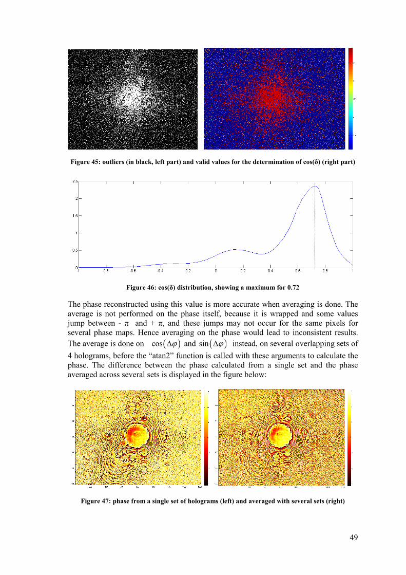
49
Figure 45: outliers (in black, left part) and valid values for the determination of cos(δ) (right part)
Figure 46: cos(δ) distribution, showing a maximum for 0.72
The phase reconstructed using this value is more accurate when averaging is done. The
average is not performed on the phase itself, because it is wrapped and some values
jump between - π and + π, and these jumps may not occur for the same pixels for
several phase maps. Hence averaging on the phase would lead to inconsistent results.
The average is done on ( )cos ϕ∆ and ( )sin ϕ∆ instead, on several overlapping sets of
4 holograms, before the “atan2” function is called with these arguments to calculate the
phase. The difference between the phase calculated from a single set and the phase
averaged across several sets is displayed in the figure below:
Figure 47: phase from a single set of holograms (left) and averaged with several sets (right)
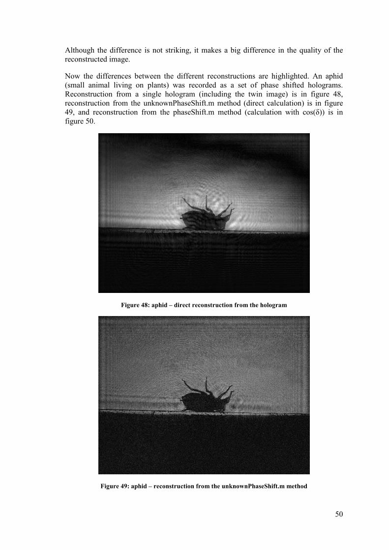
50
Although the difference is not striking, it makes a big difference in the quality of the
reconstructed image.
Now the differences between the different reconstructions are highlighted. An aphid
(small animal living on plants) was recorded as a set of phase shifted holograms.
Reconstruction from a single hologram (including the twin image) is in figure 48,
reconstruction from the unknownPhaseShift.m method (direct calculation) is in figure
49, and reconstruction from the phaseShift.m method (calculation with cos(δ)) is in
figure 50.
Figure 48: aphid – direct reconstruction from the hologram
Figure 49: aphid – reconstruction from the unknownPhaseShift.m method
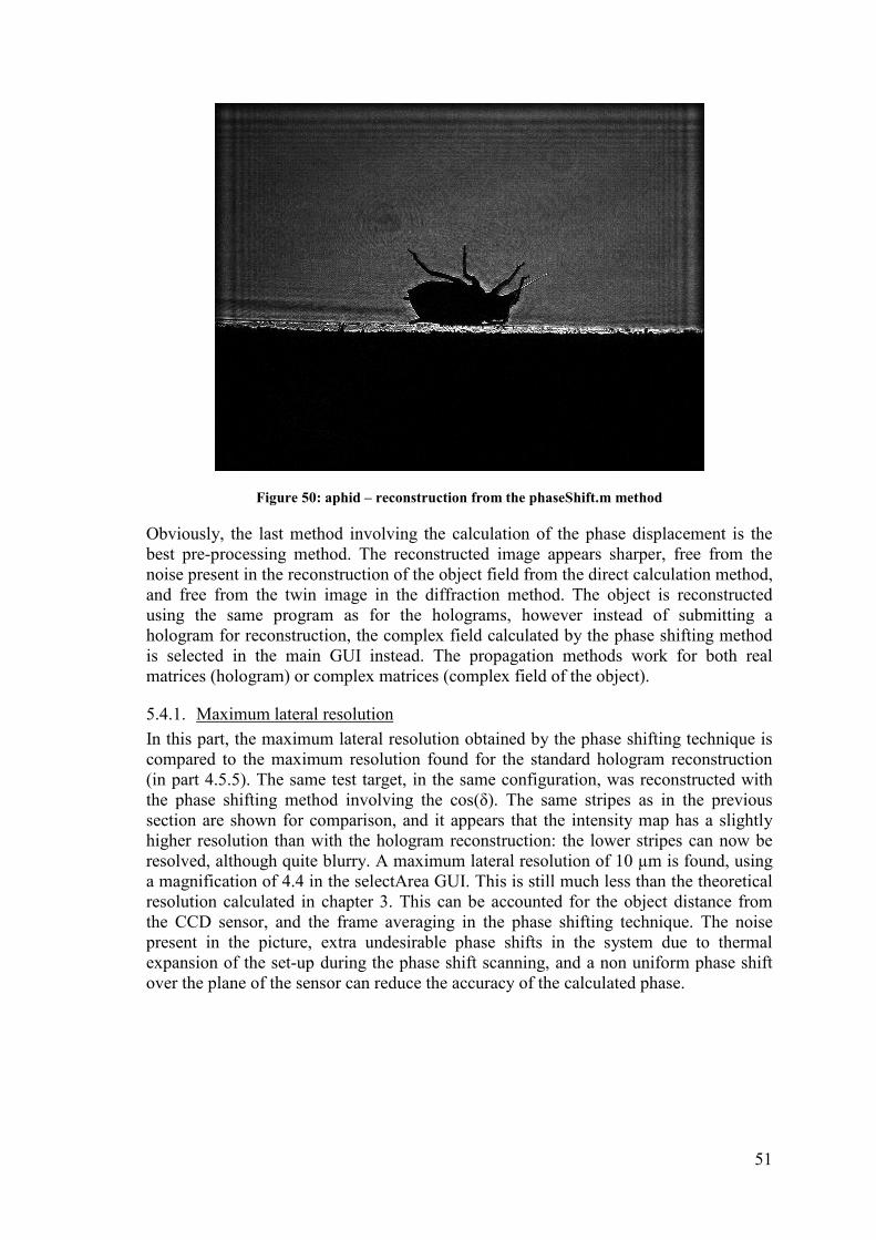
51
Figure 50: aphid – reconstruction from the phaseShift.m method
Obviously, the last method involving the calculation of the phase displacement is the
best pre-processing method. The reconstructed image appears sharper, free from the
noise present in the reconstruction of the object field from the direct calculation method,
and free from the twin image in the diffraction method. The object is reconstructed
using the same program as for the holograms, however instead of submitting a
hologram for reconstruction, the complex field calculated by the phase shifting method
is selected in the main GUI instead. The propagation methods work for both real
matrices (hologram) or complex matrices (complex field of the object).
5.4.1. Maximum lateral resolution
In this part, the maximum lateral resolution obtained by the phase shifting technique is
compared to the maximum resolution found for the standard hologram reconstruction
(in part 4.5.5). The same test target, in the same configuration, was reconstructed with
the phase shifting method involving the cos(δ). The same stripes as in the previous
section are shown for comparison, and it appears that the intensity map has a slightly
higher resolution than with the hologram reconstruction: the lower stripes can now be
resolved, although quite blurry. A maximum lateral resolution of 10 µm is found, using
a magnification of 4.4 in the selectArea GUI. This is still much less than the theoretical
resolution calculated in chapter 3. This can be accounted for the object distance from
the CCD sensor, and the frame averaging in the phase shifting technique. The noise
present in the picture, extra undesirable phase shifts in the system due to thermal
expansion of the set-up during the phase shift scanning, and a non uniform phase shift
over the plane of the sensor can reduce the accuracy of the calculated phase.
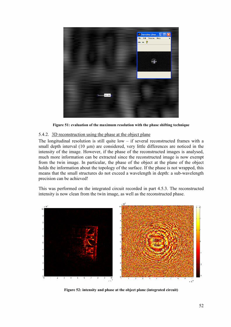
52
Figure 51: evaluation of the maximum resolution with the phase shifting technique
5.4.2. 3D reconstruction using the phase at the object plane
The longitudinal resolution is still quite low – if several reconstructed frames with a
small depth interval (10 µm) are considered, very little differences are noticed in the
intensity of the image. However, if the phase of the reconstructed images is analysed,
much more information can be extracted since the reconstructed image is now exempt
from the twin image. In particular, the phase of the object at the plane of the object
holds the information about the topology of the surface. If the phase is not wrapped, this
means that the small structures do not exceed a wavelength in depth: a sub-wavelength
precision can be achieved!
This was performed on the integrated circuit recorded in part 4.5.3. The reconstructed
intensity is now clean from the twin image, as well as the reconstructed phase.
Figure 52: intensity and phase at the object plane (integrated circuit)
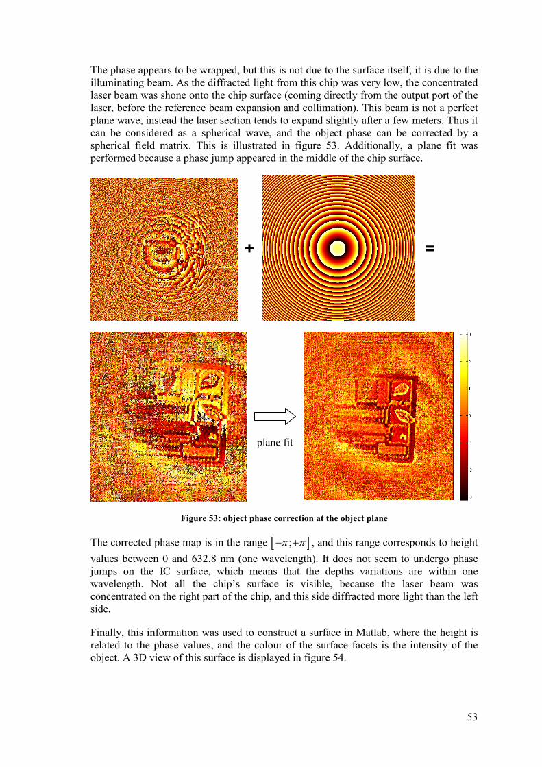
53
The phase appears to be wrapped, but this is not due to the surface itself, it is due to the
illuminating beam. As the diffracted light from this chip was very low, the concentrated
laser beam was shone onto the chip surface (coming directly from the output port of the
laser, before the reference beam expansion and collimation). This beam is not a perfect
plane wave, instead the laser section tends to expand slightly after a few meters. Thus it
can be considered as a spherical wave, and the object phase can be corrected by a
spherical field matrix. This is illustrated in figure 53. Additionally, a plane fit was
performed because a phase jump appeared in the middle of the chip surface.
Figure 53: object phase correction at the object plane
The corrected phase map is in the range [ ];π π− + , and this range corresponds to height
values between 0 and 632.8 nm (one wavelength). It does not seem to undergo phase
jumps on the IC surface, which means that the depths variations are within one
wavelength. Not all the chip’s surface is visible, because the laser beam was
concentrated on the right part of the chip, and this side diffracted more light than the left
side.
Finally, this information was used to construct a surface in Matlab, where the height is
related to the phase values, and the colour of the surface facets is the intensity of the
object. A 3D view of this surface is displayed in figure 54.
+ =
plane fit
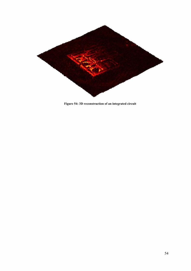
54
Figure 54: 3D reconstruction of an integrated circuit
55
Conclusion
The discovery and the implementation of some holographic reconstruction techniques
were of very high interest. Some issues were encountered from the theoretical point of
view and the practical use of the techniques, and solutions were found to overcome
them. Eventually, consistent results were obtained, providing a confirmation for the
expected improvements from the modifications brought to the optical set-up and the
numerical algorithms.
The lateral resolution remains lower than the one expected. This parameter could be
improved by using a CCD sensor with a smaller spatial sampling, or inter-pixel distance
(lowers the minimum distance between the object and the CCD sensor). Also, a wider
CCD sensor area allows for a bigger numerical aperture (but increases the minimum
distance). The use of a lens between the object and the CCD sensor lowers the spatial
frequencies on the CCD sensor, enabling to record an object at a smaller distance; but it
reduces the resolution.
The phase shifting technique is the most promising, enabling much sharper and cleaner
images reconstruction. It requires more experimental work for the holograms recording
and needs very precise tools for shifting the phase, but this is worthwhile because more
information can be recovered and a better object reconstruction is achieved.
Additionally, a 3D reconstruction of a surface topology becomes possible with the use
of the phase at the object plane, as the information for the depth. This was not possible
with the hologram reconstruction, because of the overlap of the real image and the
propagated field from the virtual image in space.
The reconstructed images are single colour images, because of the use of a single laser.
Full colour images could be obtained with an optical set-up including three lasers (red,
green and blue), combining these beams with beam splitters, and using a colour CCD
sensor to record three holograms at the same time. The numerical processing would
require three times more time or computing power; however such a holographic
microscope would equal or even surpass a conventional microscope thanks to the ability
to refocus the image as required, after the recording process.
56
References
Books
[1] Gori, F. (1995), Elementi Di Ottica, Roma: Accademica, ISBN 88-85929-06-0
[2] Schnars, U., & Juptner, W. (2004), Digital Holography, Berlin Heidelberg:
Springer Verlag, ISBN 3-540-21934-x
[3] Kreis, T. (2004), Handbook of Holographic Interferometry, Weinheim:
WILEY-VCH Verlag GmbH & Co.KGaA, ISBN: 3-527-40546-1
[4] Hariharan, P. (2002), Basics of Holography, Cambridge: Cambridge
University Press, ISBN: 0-521-00200-1
[5] Kasper, J. E. & Feller, S. A. (1985), The complete book of holograms – How
they work and how to make them, New York: Wiley, John & Sons,
Incorporated, ISBN: 0-471-62941-3
[6] Press, William H., Flannery, Brian P., Teukolsky, Saul A., Vetterling,
William T. (1986), Numerical recipes, Cambridge: Cambridge University
Press, ISBN: 0-521-30811-9
From Internet
[7] Mathworks website – Matlab Central: “Multicore - Parallel processing on
multiple cores” by Markus Buehren, freely downloadable, last access:
09/08/2009
http://www.mathworks.com/matlabcentral/fileexchange/13775
[8] High precision deformation measurement by digital phase shifting holographic
interferometry – by Ming Chang, Ching-Piao Hu, Philip Lam, and James C.
Wyant, last access: 09/08/2009
http://www.optics.arizona.edu/jcwyant/pdf/Published_Papers/Phase_Shifting/Hig
hPrecisionDeformationMeasurementByDigitalPhaseShiftingHolographicInterfer
ometry.pdf
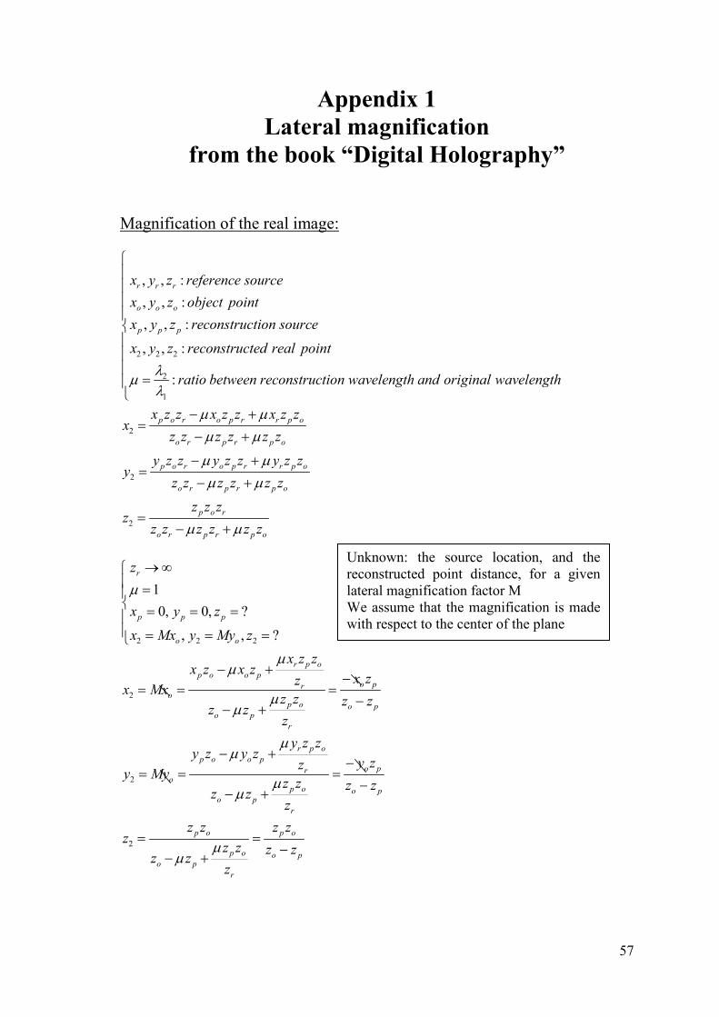
57
Appendix 1 Lateral magnification
from the book “Digital Holography”
Magnification of the real image:
2 2 2
2
1
2
, , :
, , :
, , :
, , :
:
r r r
o o o
p p p
p o r o p r r
x y z reference source
x y z object point
x y z reconstruction source
x y z reconstructed real point
ratio between reconstruction wavelength and original wavelength
x z z x z z xx
λµ
λ
µ µ
=
− +=
2
2
p o
o r p r p o
p o r o p r r p o
o r p r p o
p o r
o r p r p o
z z
z z z z z z
y z z y z z y z zy
z z z z z z
z z zz
z z z z z z
µ µ
µ µ
µ µ
µ µ
− +
− +=
− +
=− +
2 2 2
2
2
2
1
0, 0, ?
, , ?
r
p p p
o o
r p o
p o o po pr
op o o p
o p
r
r p o
p o o po pr
op o o p
o p
r
p o p o
p o o po p
r
z
x y z
x Mx y My z
x z zx z x z
x zzx Mx
z z z zz z
z
y z zy z y z
y zzy My
z z z zz z
z
z z z zz
z z z zz z
z
µ
µµ
µµ
µµ
µµ
µµ
→∞ = = = = = = =
− +−
= = =−
− +
− +−
= = =−
− +
= =−
− +
Unknown: the source location, and the
reconstructed point distance, for a given
lateral magnification factor M
We assume that the magnification is made
with respect to the center of the plane
58
( )
( )2 1
2
2
2
1
1 1
1
1 1
p op o p p
p o
p o
o p p o
o p
o oo o
oo o
o
z MzM M z z z z
z z M
z zz z z z z z
z z
Mz Mzz z z
M M
MzM Mz z z
M M
z Mz
= ⇒ − = ⇒ =
− − = ⇒ − = −
− = − −
− − = − −
= −
Magnification of the virtual image:
1 1 1
2
1
1
, , :
, , :
, , :
, , :
:
r r r
o o o
p p p
p o r o p r
x y z reference source
x y z object point
x y z reconstruction source
x y z reconstructed virtual point
ratio between reconstruction wavelength and original wavelength
x z z x z zx
λµ
λ
µ
=
+ −=
1
1
r p o
o r p r p o
p o r o p r r p o
o r p r p o
p o r
o r p r p o
x z z
z z z z z z
y z z y z z y z zy
z z z z z z
z z zz
z z z z z z
µ
µ µ
µ µ
µ µ
µ µ
+ −
+ −=
+ −
=+ −
The plane wave reference source is considered as a point source of light located at the
infinity. The ratio between the reconstruction wavelength and the original wavelength is
kept at one to ensure that the reconstruction is made with the same wavelength. This
parameter influences the longitudinal dimension but not the lateral dimensions.
59
1 1 1
1
1
1
1
0, 0, ?
, , ?
r
p p p
o o
r p o
p o o po pr
op o o p
o p
r
r p o
p o o po pr
op o o p
o p
r
p o p o
p o o po p
r
z
x y z
x Mx y My z
x z zx z x z
x zzx Mx
z z z zz z
z
y z zy z y z
y zzy My
z z z zz z
z
z z z zz
z z z zz z
z
µ
µµ
µµ
µµ
µµ
µµ
→∞ = = = = = = =
+ −= = =
++ −
+ −= = =
++ −
= =+
+ −
( )
( )1 1
1
1
1
1
1 1
1
1 1
p oo p p p
o p
p o
o p p o
o p
o oo o
oo o
o
z MzM M z z z z
z z M
z zz z z z z z
z z
Mz Mzz z z
M M
MzM Mz z z
M M
z Mz
= ⇒ + = ⇒ =
+ − = ⇒ + = +
+ = − −
− + = − −
=
Unknown: the source location, and the
reconstructed point distance, for a given
lateral magnification factor M
We assume that the magnification is made
with respect to the center of the plane
60
Appendix 2 π/2 phase shift method
( )
( )
( )
( ) ( )
1
2
3
4
cos sin2
cos
cos sin2
cos cos
I A B A B
I A B
I A B A B
I A B A B
πϕ ϕ
ϕ
πϕ ϕ
ϕ π ϕ
= + ∆ − = + ∆ = + ∆
= + ∆ + = − ∆
= + ∆ + = − ∆
( )
( )
1 3
2 4
sin2
cos2
I IB
I IB
ϕ
ϕ
− ∆ =
− ∆ =
The phase is calculated by doing ( )( )
sinarctan
cos
B
B
ϕϕ
ϕ
∆∆ = ∆
and adding π if
( )cos 0ϕ∆ < . Alternatively, the “atan2” function in Matlab can directly calculate the
angle in the [-π ; +π ] range: atan2( ( )sinB ϕ∆ , ( )cosB ϕ∆ ).
If even more holograms are recorded, more
averaging can be performed to reduce the noise
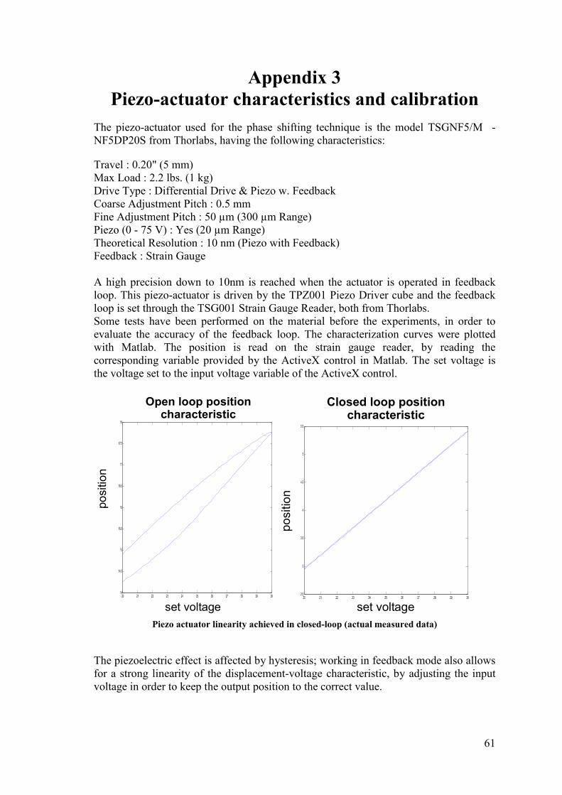
61
Appendix 3 Piezo-actuator characteristics and calibration
The piezo-actuator used for the phase shifting technique is the model TSGNF5/M -
NF5DP20S from Thorlabs, having the following characteristics:
Travel : 0.20" (5 mm)
Max Load : 2.2 lbs. (1 kg)
Drive Type : Differential Drive & Piezo w. Feedback
Coarse Adjustment Pitch : 0.5 mm
Fine Adjustment Pitch : 50 µm (300 µm Range)
Piezo (0 - 75 V) : Yes (20 µm Range)
Theoretical Resolution : 10 nm (Piezo with Feedback)
Feedback : Strain Gauge
A high precision down to 10nm is reached when the actuator is operated in feedback
loop. This piezo-actuator is driven by the TPZ001 Piezo Driver cube and the feedback
loop is set through the TSG001 Strain Gauge Reader, both from Thorlabs.
Some tests have been performed on the material before the experiments, in order to
evaluate the accuracy of the feedback loop. The characterization curves were plotted
with Matlab. The position is read on the strain gauge reader, by reading the
corresponding variable provided by the ActiveX control in Matlab. The set voltage is
the voltage set to the input voltage variable of the ActiveX control.
Open loop positioncharacteristic
set voltage
position
Closed loop positioncharacteristic
position
set voltage
Piezo actuator linearity achieved in closed-loop (actual measured data)
The piezoelectric effect is affected by hysteresis; working in feedback mode also allows
for a strong linearity of the displacement-voltage characteristic, by adjusting the input
voltage in order to keep the output position to the correct value.
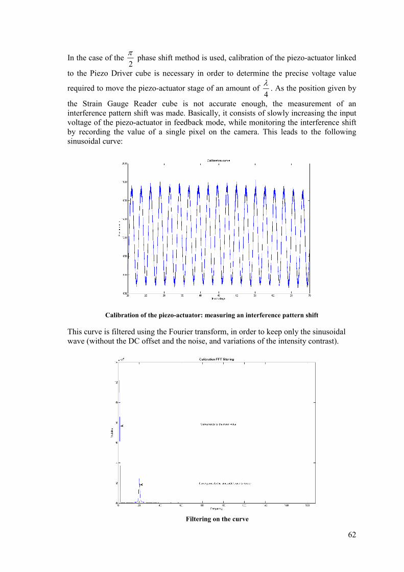
62
In the case of the 2
π phase shift method is used, calibration of the piezo-actuator linked
to the Piezo Driver cube is necessary in order to determine the precise voltage value
required to move the piezo-actuator stage of an amount of 4
λ. As the position given by
the Strain Gauge Reader cube is not accurate enough, the measurement of an
interference pattern shift was made. Basically, it consists of slowly increasing the input
voltage of the piezo-actuator in feedback mode, while monitoring the interference shift
by recording the value of a single pixel on the camera. This leads to the following
sinusoidal curve:
Calibration of the piezo-actuator: measuring an interference pattern shift
This curve is filtered using the Fourier transform, in order to keep only the sinusoidal
wave (without the DC offset and the noise, and variations of the intensity contrast).
Filtering on the curve
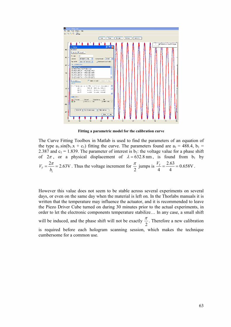
63
Fitting a parametric model for the calibration curve
The Curve Fitting Toolbox in Matlab is used to find the parameters of an equation of
the type a1.sin(b1.x + c1) fitting the curve. The parameters found are a1 = 488.4, b1 =
2.387 and c1 = 1.839. The parameter of interest is b1: the voltage value for a phase shift
of 2π , or a physical displacement of 632.8 nmλ = , is found from b1 by
1
22.63VTV
b
π= = . Thus the voltage increment for
2
π jumps is
2.630.658V
4 4
TV = = .
However this value does not seem to be stable across several experiments on several
days, or even on the same day when the material is left on. In the Thorlabs manuals it is
written that the temperature may influence the actuator, and it is recommended to leave
the Piezo Driver Cube turned on during 30 minutes prior to the actual experiments, in
order to let the electronic components temperature stabilize… In any case, a small shift
will be induced, and the phase shift will not be exactly 2
π. Therefore a new calibration
is required before each hologram scanning session, which makes the technique
cumbersome for a common use.
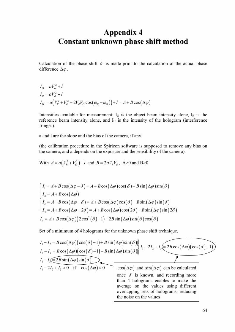
64
Appendix 4 Constant unknown phase shift method
Calculation of the phase shift δ is made prior to the calculation of the actual phase
difference ϕ∆ .
( )( ) ( )
2
2
2 2 2 cos cos
O o
R R
H R O R O R O
I aV l
I aV l
I a V V V V l A Bϕ ϕ ϕ
= +
= +
= + + − + = + ∆
Intensities available for measurement: IO is the object beam intensity alone, IR is the
reference beam intensity alone, and IH is the intensity of the hologram (interference
fringes).
a and l are the slope and the bias of the camera, if any.
(the calibration procedure in the Spiricon software is supposed to remove any bias on
the camera, and a depends on the exposure and the sensibility of the camera).
With ( )2 2
R OA a V V l= + + and 2 R OB aV V= , A>0 and B>0
( ) ( ) ( ) ( ) ( )( )( ) ( ) ( ) ( ) ( )( ) ( ) ( ) ( ) ( )
( ) ( )( ) ( ) ( ) ( )
1
2
3
4
2
4
cos cos cos sin sin
cos
cos cos cos sin sin
cos 2 cos cos 2 sin sin 2
cos 2cos 1 2 sin sin cos
I A B A B B
I A B
I A B A B B
I A B A B B
I A B B
ϕ δ ϕ δ ϕ δ
ϕ
ϕ δ ϕ δ ϕ δ
ϕ δ ϕ δ ϕ δ
ϕ δ ϕ δ δ
= + ∆ − = + ∆ + ∆
= + ∆
= + ∆ + = + ∆ − ∆ = + ∆ + = + ∆ − ∆
= + ∆ − − ∆
Set of a minimum of 4 holograms for the unknown phase shift technique.
( ) ( )( ) ( ) ( )( ) ( )( ) ( ) ( )
( ) ( )( )
( ) ( )( )
1 2
1 2 3
3 2
1 3
1 2 3
cos cos 1 sin sin2 2 cos cos 1
cos cos 1 sin sin
2 sin sin
2 0 if cos 0
I I B BI I I B
I I B B
I I B
I I I
ϕ δ ϕ δϕ δ
ϕ δ ϕ δ
ϕ δ
ϕ
− = ∆ − + ∆ − + = ∆ −
− = ∆ − − ∆ − = ∆
− + > ∆ <
( )cos ϕ∆ and ( )sin ϕ∆ can be calculated
once δ is known, and recording more
than 4 holograms enables to make the
average on the values using different
overlapping sets of holograms, reducing
the noise on the values
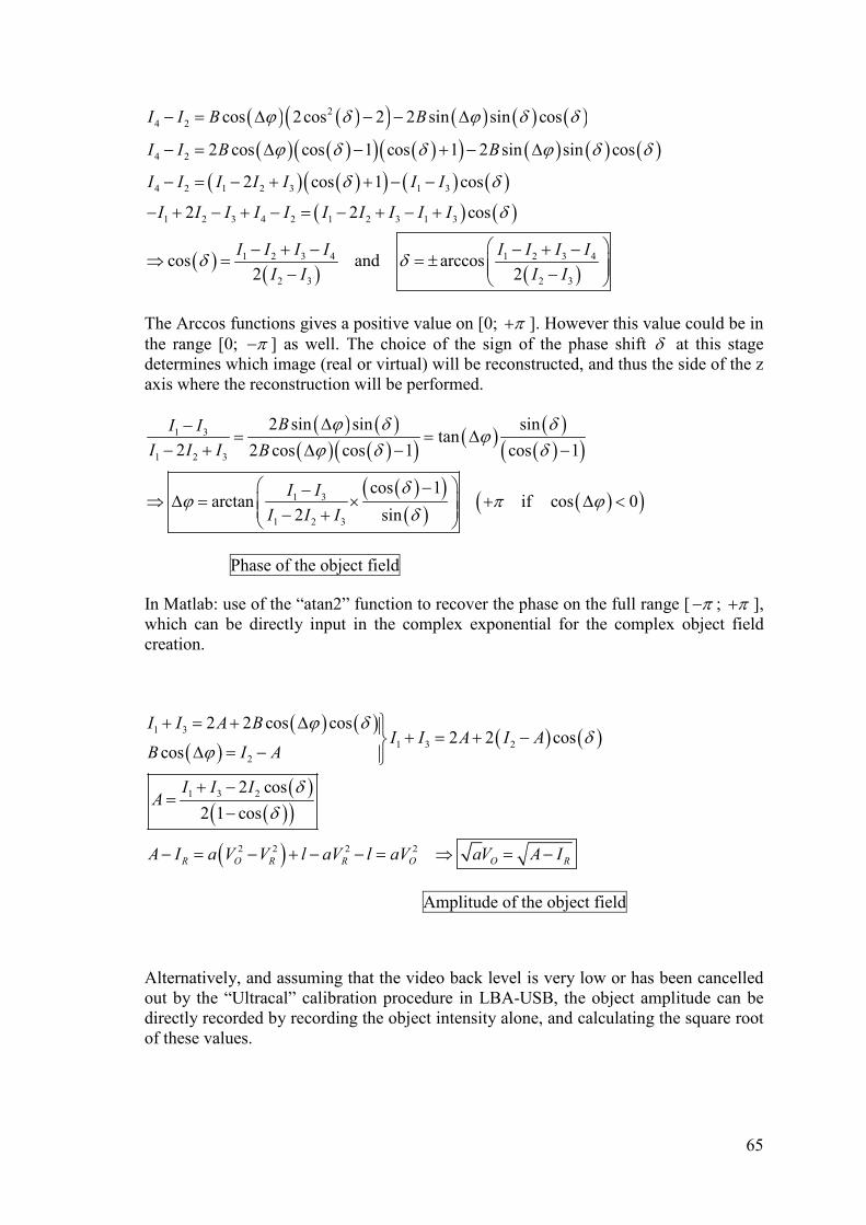
65
( ) ( )( ) ( ) ( ) ( )
( ) ( )( ) ( )( ) ( ) ( ) ( )( ) ( )( ) ( ) ( )
( ) ( )
( )( ) ( )
2
4 2
4 2
4 2 1 2 3 1 3
1 2 3 4 2 1 2 3 1 3
1 2 3 4 1 2 3 4
2 3 2 3
cos 2cos 2 2 sin sin cos
2 cos cos 1 cos 1 2 sin sin cos
2 cos 1 cos
2 2 cos
cos and arccos2 2
I I B B
I I B B
I I I I I I I
I I I I I I I I I I
I I I I I I I I
I I I I
ϕ δ ϕ δ δ
ϕ δ δ ϕ δ δ
δ δ
δ
δ δ
− = ∆ − − ∆
− = ∆ − + − ∆
− = − + + − −
− + − + − = − + − +
− + − − + −⇒ = = ± − −
The Arccos functions gives a positive value on [0; π+ ]. However this value could be in
the range [0; π− ] as well. The choice of the sign of the phase shift δ at this stage
determines which image (real or virtual) will be reconstructed, and thus the side of the z
axis where the reconstruction will be performed.
( ) ( )( ) ( )( ) ( ) ( )
( )( )( )( )( )
( )( )
1 3
1 2 3
1 3
1 2 3
2 sin sin sintan
2 2 cos cos 1 cos 1
cos 1arctan if cos 0
2 sin
BI I
I I I B
I I
I I I
ϕ δ δϕ
ϕ δ δ
δϕ π ϕ
δ
∆−= = ∆
− + ∆ − −
−−⇒ ∆ = × + ∆ < − +
Phase of the object field
In Matlab: use of the “atan2” function to recover the phase on the full range [ π− ; π+ ],
which can be directly input in the complex exponential for the complex object field
creation.
( ) ( )( )
( ) ( )
( )( )( )
( )
1 3
1 3 2
2
1 3 2
2 2 2 2
2 2 cos cos2 2 cos
cos
2 cos
2 1 cos
R O R R O O R
I I A BI I A I A
B I A
I I IA
A I a V V l aV l aV aV A I
ϕ δδ
ϕ
δδ
+ = + ∆ + = + −∆ = −
+ −=
−
− = − + − − = ⇒ = −
Amplitude of the object field
Alternatively, and assuming that the video back level is very low or has been cancelled
out by the “Ultracal” calibration procedure in LBA-USB, the object amplitude can be
directly recorded by recording the object intensity alone, and calculating the square root
of these values.
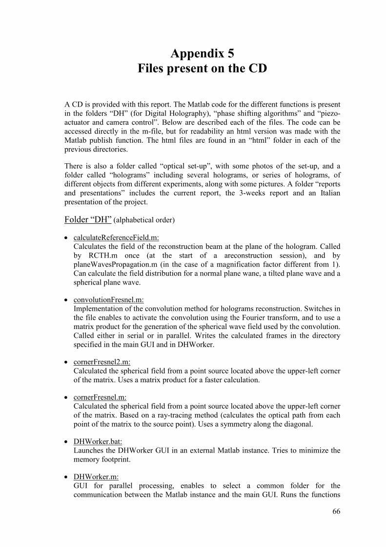
66
Appendix 5 Files present on the CD
A CD is provided with this report. The Matlab code for the different functions is present
in the folders “DH” (for Digital Holography), “phase shifting algorithms” and “piezo-
actuator and camera control”. Below are described each of the files. The code can be
accessed directly in the m-file, but for readability an html version was made with the
Matlab publish function. The html files are found in an “html” folder in each of the
previous directories.
There is also a folder called “optical set-up”, with some photos of the set-up, and a
folder called “holograms” including several holograms, or series of holograms, of
different objects from different experiments, along with some pictures. A folder “reports
and presentations” includes the current report, the 3-weeks report and an Italian
presentation of the project.
Folder “DH” (alphabetical order)
• calculateReferenceField.m:
Calculates the field of the reconstruction beam at the plane of the hologram. Called
by RCTH.m once (at the start of a areconstruction session), and by
planeWavesPropagation.m (in the case of a magnification factor different from 1).
Can calculate the field distribution for a normal plane wane, a tilted plane wave and a
spherical plane wave.
• convolutionFresnel.m:
Implementation of the convolution method for holograms reconstruction. Switches in
the file enables to activate the convolution using the Fourier transform, and to use a
matrix product for the generation of the spherical wave field used by the convolution.
Called either in serial or in parallel. Writes the calculated frames in the directory
specified in the main GUI and in DHWorker.
• cornerFresnel2.m:
Calculated the spherical field from a point source located above the upper-left corner
of the matrix. Uses a matrix product for a faster calculation.
• cornerFresnel.m:
Calculated the spherical field from a point source located above the upper-left corner
of the matrix. Based on a ray-tracing method (calculates the optical path from each
point of the matrix to the source point). Uses a symmetry along the diagonal.
• DHWorker.bat:
Launches the DHWorker GUI in an external Matlab instance. Tries to minimize the
memory footprint.
• DHWorker.m:
GUI for parallel processing, enables to select a common folder for the
communication between the Matlab instance and the main GUI. Runs the functions
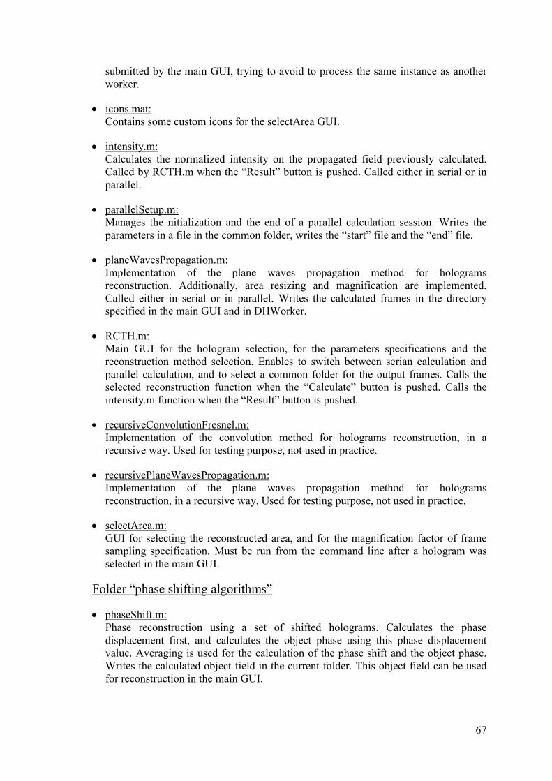
67
submitted by the main GUI, trying to avoid to process the same instance as another
worker.
• icons.mat:
Contains some custom icons for the selectArea GUI.
• intensity.m:
Calculates the normalized intensity on the propagated field previously calculated.
Called by RCTH.m when the “Result” button is pushed. Called either in serial or in
parallel.
• parallelSetup.m:
Manages the nitialization and the end of a parallel calculation session. Writes the
parameters in a file in the common folder, writes the “start” file and the “end” file.
• planeWavesPropagation.m:
Implementation of the plane waves propagation method for holograms
reconstruction. Additionally, area resizing and magnification are implemented.
Called either in serial or in parallel. Writes the calculated frames in the directory
specified in the main GUI and in DHWorker.
• RCTH.m:
Main GUI for the hologram selection, for the parameters specifications and the
reconstruction method selection. Enables to switch between serian calculation and
parallel calculation, and to select a common folder for the output frames. Calls the
selected reconstruction function when the “Calculate” button is pushed. Calls the
intensity.m function when the “Result” button is pushed.
• recursiveConvolutionFresnel.m:
Implementation of the convolution method for holograms reconstruction, in a
recursive way. Used for testing purpose, not used in practice.
• recursivePlaneWavesPropagation.m:
Implementation of the plane waves propagation method for holograms
reconstruction, in a recursive way. Used for testing purpose, not used in practice.
• selectArea.m:
GUI for selecting the reconstructed area, and for the magnification factor of frame
sampling specification. Must be run from the command line after a hologram was
selected in the main GUI.
Folder “phase shifting algorithms”
• phaseShift.m:
Phase reconstruction using a set of shifted holograms. Calculates the phase
displacement first, and calculates the object phase using this phase displacement
value. Averaging is used for the calculation of the phase shift and the object phase.
Writes the calculated object field in the current folder. This object field can be used
for reconstruction in the main GUI.
68
• unknownPhaseShift.m:
Phase reconstruction using a set of shifted holograms. Direct calculation of the object
phase. Problems due to outliers, and frame averaging is not correct. Writes the
calculated object field in the current folder.
Folder “piezo-actuator and camera control”
• piezoDriver.m:
Complete automation of the phase shifting scanning. Controls the hardware
(piezoelectric actuator and digital camera) through the use of ActiveX controls
within Matlab. Two modes are implemented: piezo-actuator calibration (sinusoidal
curve from a shifted interference pattern), and the actual phase shifting (holograms
recording). Calls the phase reconstruction function at the end of the holograms
recording session.
69
Appendix 6 Example of holographic reconstruction
1-1) Hologram of a mosquito:
1-2) Direct reconstruction from the hologram
(mixed real image and propagated virtual image):
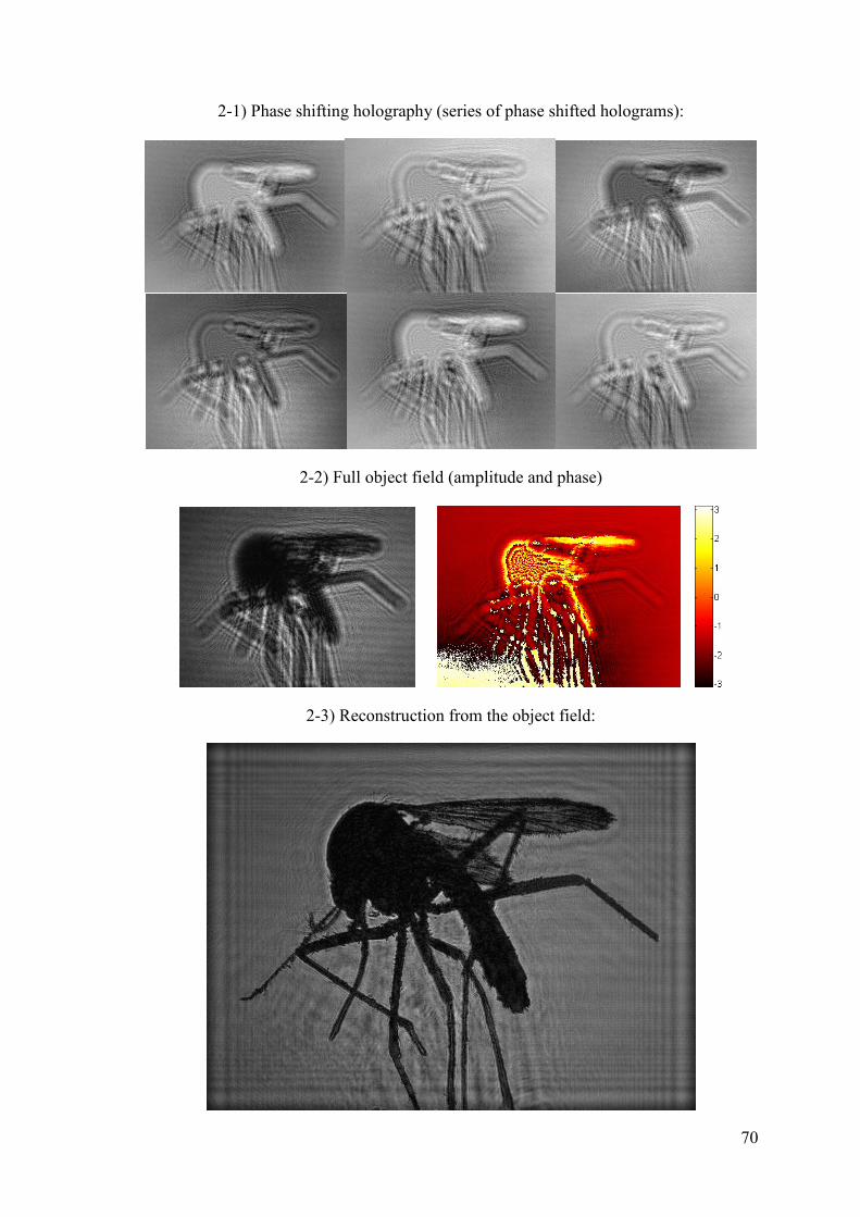
70
2-1) Phase shifting holography (series of phase shifted holograms):
2-2) Full object field (amplitude and phase)
2-3) Reconstruction from the object field:
Summary
This report describes the work made on the digital holography techniques for the optical
microscopy, in the frame of my Master’s internship.
Holograms of microscopic objects were recorded with a digital camera and virtually
reconstructed in space on a computer. Main targets were the precision of the
reconstruction, the reconstructed picture resolution and the management of the
computing resources involved for the propagation calculation. In order to facilitate the
selection of the hologram and of the reconstruction parameters, a graphical user
interface was created for the reconstruction program.
Different optical field propagation methods were implemented on Matlab. The
possibility of selecting an area to reconstruct as well as the use of a magnification factor
were added afterwards.
A different technique was used at the end of the internship. Using several holograms
recorded with an increasing phase shift of the reference beam, it was possible to
calculate the complex object field at the plane of the hologram. The propagation of this
object field with the same techniques as above lead to a better object reconstruction.
Moreover, a three-dimensional visualization of a microscopic surface depth was made
possible by using this technique.
Résumé
Ce rapport décrit le travail effectué sur l’holographie digitale pour la microscopie
optique, dans le cadre de mon stage de Master.
Des hologrammes d’objets microscopiques ont été enregistrés avec une caméra
numérique et ont été reconstruits virtuellement dans l’espace sur un ordinateur. Les
principaux objectifs visés étaient la précision de la reconstruction, la résolution de
l’image reconstruite et la gestion des ressources de l’ordinateur mises en jeu lors du
calcul de la propagation. De façon a faciliter la sélection de l’hologramme et des
paramètres de reconstruction, une interface graphique a été créée pour le programme de
reconstruction.
Differentes méthodes de propagation d’un champ optique ont été appliquées sur Matlab.
La possibilité de sélectionner une zone à reconstruire ainsi que l’usage d’un facteur
d’agrandissement ont été ajoutés par la suite.
Une technique différente a été utilisée à la fin du stage. En utilisant plusieurs
hologrammes enregistrés avec un déplacement de phase croissant du rayon de référence,
il a été possible de calculer le champ complexe de l’objet sur le plan de l’hologramme.
La propagation du champ de l’objet avec les mêmes techniques que précédemment a
conduit à une meilleure reconstruction de l’objet. De plus, la visualisation en trois
dimensions du relief d’une surface microscopique a été rendue possible par l’usage de
cette technique.