z)?3z- - dtic

REPORT DOCUMENTATION PAGE

Public reporting burden far this collection of information is estimated to average 1 hour per response, including the time for reviewing instructions, sea the collection of information. Send comments regarding this burden estimate or any other aspect of this collection of information, including sugg _ j Q-p T>T -"T'R-OO" Operations and Reports, 1215 Jefferson Davis Highway, Suite 1204, Arlington, VA 22202-4302, and to the Office of Management and Budget, Pape p^ KJ^"^-CS-"-LJJ-J

'eviewmg ormation

1. AGENCY USE ONLY /Leaveblank/ REPORT DATE *~

December, 1996 3. REPOF

Z)?3Z- 4. TITLE AND SUBTITLE

1996 Summer Research Program (SRP), Summer Faculty Research Program (SFRP), Final Reports, Volume 5A, Wright Laboratory

6. AUTHOR(S)

Gary Moore

7. PERFORMING ORGANIZATION NAME(S) AND ADDRESS(ES)

Research & Development Laboratories (RDL)

5800 Uplander Way Culver City, CA 90230-6608

9. SPONSORING/MONITORING AGENCY NAME(S) AND ADDRESS(ES)

Air Force Office of Scientific Research (AFOSR)

801 N. Randolph St. Arlington, VA 22203-1977

9. FUNDING NUMBERS

F49620-93-C-0063

8. PERFORMING ORGANIZATION REPORT NUMBER

10. SPONSORING/MONITORING AGENCY REPORT NUMBER

11. SUPPLEMENTARY NOTES

12a. DISTRIBUTION AVAILABILITY STATEMENT

Approved for Public Release

12b. DISTRIBUTION CODE

13. ABSTRACT (Maximum 200 words)

The United States Air Force Summer Research Program (USAF-SRP) is designed to introduce university, college, and technical institute faculty members, graduate students, and high school students to Air Force research. This is accomplished by the faculty members (Summer Faculty Research Program, (SFRP)), graduate students (Graduate Student Research Program (GSRP)), and high school students (High School Apprenticeship Program (HSAP)) being selected on a nationally advertised competitive basis during the summer intersession period to perform research at Air Force Research Laboratory (AFRL) Technical Directorates, Air Force Air Logistics Centers (ALC), and other AF Laboratories. This volume consists of a program overview, program management statistics, and the final technical reports from the SFRP participants at the Wright Laboratory.

14. SUBJECT TERMS

Air Force Research, Air Force, Engineering, Laboratories, Reports, Summer, Universities, Faculty, Graduate Student, High School Student

15. NUMBER OF PAGES

16. PRICE CODE

17. SECURITY CLASSIFICATION OF REPORT

Unclassified

18. SECURITY CLASSIFICATION OF THIS PAGE

Unclassified

19. SECURITY CLASSIFICATION OF ABSTRACT

Unclassified

20. LIMITATION OF ABSTRACT

UL Standard Form 298 (Rev. 2-89) (EG) Prescribed by ANSI Std. 239.18 Designed using Perform Pro, WHS/DIOR, Oct 94

UNITED STATES AIR FORCE

SUMMER RESEARCH PROGRAM - 1996

SUMMER FACULTY RESEARCH PROGRAM FINAL REPORTS

VOLUME 5A

WRIGHT LABORATORY

RESEARCH & DEVELOPMENT LABORATORIES

5800 Upiander Way

Culver City, CA 90230-6608

Program Director, RDL Program Manager, AFOSR Gary Moore Major Linda Steel-Goodwin

Program Manager, RDL Program Administrator, RDL Scott Licoscos Johnetta Thompson

Program Administrator, RDL Rebecca Kelly

Submitted to:

AIR FORCE OFFICE OF SCIENTIFIC RESEARCH

Boiling Air Force Base

Washington, D.C.

December 1996

{\(\ fA Ol" Ok" /a*fc

PREFACE

Reports in this volume are numbered consecutively beginning with number 1. Each report is paginated with the report number followed by consecutive page numbers, e.g., 1-1, 1-2, 1-3; 2-1, 2-2,

2-3.

Due to its length, Volume 5 is bound in three parts, 5A, 5B and 5C. Volume 5A contains #1-24. Volume 5B contains reports #25-48 and 5C contains #49-70. The Table of Contents for

Volume 5 is included in all parts.

This document is one of a set of 16 volumes describing the 1996 AFOSR Summer Research Program. The following volumes comprise the set:

VOLUME TITLE

2A&2B

3A&3B

4

5A , 5B & 5C

6

7A&7B

8

9

10A&10B

11

12A & 12B

13

14

15A&15B

16

Program Management Report

Summer Faculty Research Program (SFRP) Reports

Armstrong Laboratory

Phillips Laboratory

Rome Laboratory

Wright Laboratory

Arnold Engineering Development Center, Wilford Hall Medical Center and

Ar Logistics Centers

Graduate Student Research Program (GSRP) Reports


Phillips Laboratory

Rome Laboratory

Wright Laboratory

Arnold Engineering Development Center, United States Ar Force Academy, Wilford Hall Medical Center, and Wright Patterson Medical Center

High School Apprenticeship Program (HSAP) Reports


Phillips Laboratory

Rome Laboratory

Wright Laboratory

Arnold Engineering Development Center

SFRP FINAL REPORT TABLE OF CONTENTS i-xviii

1. INTRODUCTION 1

2. PARTICIPATION IN THE SUMMER RESEARCH PROGRAM 2

3. RECRUITING AND SELECTION 3

4. SITE VISITS 4

5. HBCU/MI PARTICIPATION 4

6. SRP FUNDING SOURCES 5

7. COMPENSATION FOR PARTICDPATIONS 5

8. CONTENTS OF THE 1996 REPORT 6

APPENDICDES:

A. PROGRAM STATISTICAL SUMMARY A-l

B. SRP EVALUATION RESPONSES B-l

SFRP FINAL REPORTS

SRP Final Report Table of Contents

University/Institution Armstrong Laboratory Author Report Title Directorate voi-Page DRRichelleM Allen-King AL/EQC 2- 1

Washington State University, Pullman , WA Reduction Kinetics in a Batch Metallic Iron/Water SystemrEffect of Iron/Water Exposure

DR Anthony R Andrews AL/EQC 2- 2 Ohio University, Athens, OH Investigation of the Electrochemiluminescent Properties of Several Natural & Synthetic Compounds

DR Deborah L Armstrong AL/CFTO 2- 3 Univ of Texas at San Antonio, San Antonio, TX Development of A primary Cell Culture Preparation for Studying Mechanisms Governi ng Circadian Rhyth

DR Robert L Armstrong AL/CFD 2- 4 New Mexico State University , Las Cruces, NM Microparticle Bioluminescence

DR Maureen E Bronson AL/OER 2- 5 Wilkes Univ School of Pharmacy , Wilkes-Barre, PA Lack of Effect of Ultra Wideband Radiation on Pentylenetetrazol-Induced Convulsions in Rats

DR Marc L Carter, PhD, PA AL/OEO 2- 6 University of South Florida, Tampa, FL Assessment of the Reliability of Ground-Based Observers for the Detection of Aircraft

DRJer-SenChen AL/CFHV 2- 7 Wright State University, Dayton, OH A Study of Data Compression Based on Human Visual Perception

DR Cheng Cheng AL/HRM 2- 8 Johns Hopkins University, Baltimore , MD Sequential Optimization Algorithm for Personnel Assignmt Based on Cut-Off Profiles & Rev of Brogden

DR Elizabeth T Davis AL/CFHP 2- 9 Georgia Institute of Tech, Atlanta, GA Perceptual Issues in Virtual Environments & Other Simulated Displays

DR Keith FEckerman AL/OEB 2- 10 Univ of Tennessee , Knoxville, TN

DR Paul A Edwards AL/EQC 2- 11 Edinboro Univ of Pennsylvania, Edinboro , PA A Viartion Fuel Identification- Neural Network Analysis of the Concentration of Benzene and Naphtha

üKF rinai Keport Table o± Contents

University/Institution Armstrong Laboratory Author Report Title Directorate voi-page DR Randolph D Glickman ———————— _____ _—__—

Univ of Texas Health Science Center, San Antonio , TX A Study of Oxidative Reaactions Mediated by Laser-Excited Ocular Melanin

DR Ellen L Glickman-Weiss AL/CFTF _ 2- 13 Kent State University, Kent, OH The Effect of Short Duration Respiratory Musculature Training on Tactical Air Combat

DR Irwin S Goldberg AL/OES 2- 14 St Mary's Univ of San Antonio, San Antonio, TX Development of a Physiologically-Based Pharmacokinetic Model for the Uptake of Volatile Chcicals dur

DR Robert J Hi rko AL/CFHP 2- 15 University of Florida, Gainesville, FL Investigation of The Suitability of Tactile and Auditory Stimuli for use in Brain Actuated Control

ISUVPPAcct4212313(Dooley) AL/OER 2- 16 Iowa State University , Ames, IA Determination of the Influence of Ultrawideband Exposure of Rts During Early Pregnancy on Pregnancy

DR Andrew E Jackson AL/HRA 2- 17 Arizona State University , Tempe, AZ A Description of Integrated Joint Use Initiatives to Satisfy Customer Reqmts Across Govt Academia

DR John E Kalns AL/AOHR Ohio State University , Columbus , OH

DR Nandini Kantian AL/CFTS Univ of Texas at San Antonio, San Antonio , TX Modeling Decompression Sickness Using Survival Analysis Techniques

DR Antti J Koivo AL/CFBA Purdue Research Foundation, West Lafayette, IN Skill Evaluation of Human Operators

DRSukBKong AL/OEA Incarnate Word College, San Antonio, TX Aromatic Hydrocabon Components in Diesel, Jet-A And JP-8 Fuels

DRXuanKong AL/CFHP Northern Illinois University, De Kalb , TL Mental Workload Classification via Physiological Signal Processing: EOG & EEG Analyses

ii

2- 18

2- 19

2- 20

2- 21

2- 22


University/Institution Armstrong Laboratory Author Report Title Directorate vol-rage DR Charles S Lessard AL/CFTO 2- 23

Texas A & M Univ-College Station , CoUege Station, TX Preliminary Studies of Human Electroencephalogram (EEG) Correlates of GzAcceleration Tolerance

DR Audrey D Levine AL/EQC 2- 24 Utah State University, Logan , UT Biogeochemical Assessment of Natural Attenuation of JP-4 Contaminated Ground Water

DR David A Ludwig AL/AOCY 2- 25 Univ of N.C. at Greensboro, Greensboro, NC The Illusion of Control & Precision Associated w/Baseline Comparisons

DR Robert G Main AL/HRT 2- 26 Cal State Univ, Chico , Chico , CA Designing Instruction For Distance Learning

DR Phillip H Marshall AL/HRM 2- 27 Texas Tech University , Lubbock, TX Time to Contact Judgments in The Presence of Static and Dynamic Objects: A Preliminary Report

MS Sandra L McAlister AL/AO 2- 28 Stonehill College, North Easton , MA

MR Bruce V Mutter AL/EQP 2- 29 Bluefield State College, Bluefield , WV Environmental Cost Analysis:Calculating Return on Investment for Emerging Technologies

DR Sundaram Narayanan AL/HRT 2- 30 Wright State University, Dayton , OH Java-Based Application of the Model-View-Controller Framwork in Developing Interfaces to interactive

DR Karl A Perusich AL/CFHI 2- 31 Purdue University , South Bend , IN Examing Alternate Entry Points in a Problem Using Fuzzy Cognitive Maps

DRJudyLRatlifT AL/EQC 2- 32 Murray State Univ, Murray, KY A Study of The Ability of Tunicates to be used as Global Bioindicators

DR Paul D Retzlaff AL/AOCN 2- 33 Univ of Northern Colorado , Greeley , CO Computerized Neuropsychological Assessment of USAF Pilots

in


University/Institution Armstrong Laboratory Author Report Title Directorate voi-gage DR William GRixcy" AL/EQC II_________ZI__ZZ_I 2- 34

University of Houston, Houston , TX The use of Solid-Phase Microextraction (SPME) for the low level Detection of BTEX and PAHs In Aqueou

DRAliMSadegh AL/CFBE 2- 35 CUNY-City College, New York, NY Investigation of Neck Models for Predicting Human Tolerance to Accelerations

DR Kandasamy Selvavel AL/AOEP . 2- 36 Claflin College, Orangeburg, SC Truncated Bivariate Exponential Models

DR Barth FSmets AL/EQC 2- 37 University of Connecticut, Storrs, CT Biodegradation of 2-4-DNTand 2,6-DNT in Mixed Culture Aerobic Fluidized Bed Reactor and Chemostat

DR Mary Alice Smith AL/OET 2- 38 University of Georgia, Athens, GA A Study of Apoptosis During Limb Development

DR Daniel P Smith AL/EQW 2- 39 Utah State University, Logan , UT Bioremediation & its Effect on Toxicity

MR. Joseph M Stauffer AL/HRMA 2- 40 Indiana State University, Terre Haute, IN Joint Corrections for Correlation Coefficients

DR William B Stavinoha AL/AOT 2- 41 Univ of Texas Health Science Center, San Antonio, TX Studies to Identify Characterisstic Changes in the Urine Following Ingestion of Poppy seed

DR William A Stock AL/HRA 2- 42 Arizona State University, Tempe, AZ Application of Meta-Analysis to Research on Pilot Training

DR Nancy J Stone AL/HRT 2- 43 Creighton University, Omaha , NE Engagement, Involvement, and Self-Regualted Leaarnign Construct and Measurement Development to Asses

DR Brenda M Sugrue AL/HRTI 2- 44 Univ of Northern Colorado, Greeley, CO Aptitude-Attribute Interactions in Test Performance

IV


University/Institution Armstrong Laboratory Author Report Title Directorate voi-Page DR Stephen A Truhon AL/HRM 2-45

Winston-Salem State University, Winston-Saiem, NC Mechanical Specialties in the U.S. Air Force: Accession Quality & Selection Test Validity

DR Mariusz Ziejewski AL/CFBV — 2-46 North Dakota State University, Fargo, ND Validation of the Deformable Neck Model for A +Gz Acceleration


University/Institution Phillips Laboratory Author Report Title Directorate voi-Page DR Graham R Allan PL/LIDN . 3.1

New Mexico Highlands University, Las Vegas, NM Temporal and Spatial Characterization of a Synchronously-Pumped Periodically-Poled Lithium Niobate Optical

3-2

3-3

DR Brian P Beecken PL/VTRP Bethel College, St Paul, MN Testing of a Dual-Band Infrared Focal Plane Array & An Infrared Camera Sys

DR Mikhail S Belen'kii PL/LIG Georgia Inst of Technology, Atlanta, GA Tilt Sensing Technique w/Small Aperture Beam & Related Physical Phenomena

DR Asoke K Bhattacharyya PL/WSQ 3-4 Lincoln University, Jefferson City, MO Part A: Effect of Earth's Surface & Loss on the Resonant Frequencies of Buried Objects

DR Joseph M Calo PL/GPD) 3.5 Brown University, Providence, RI Transient Studies of the Effects of Fire Suppressants in a Well-Stirred Combustor

DR James J Carroll PL/WSQ 3-6 Youngstown State University, Youngstown, OH Examination of Critical Issues in the use of (178) hf For High Energy Density Applications

DRSoyoungS Cha PL/LIMS 3-7 Univ of Dlinois at Chicago, Chicago, EL A Study on Hartmann Sensor Application to Flow Aero-Optics Investigation Through Tomographie Recons

DR Tsuchin Chu PL/RKS - Southern Illinois Univ-Carbondale, Carbondale, IL

DR Kenneth Davies PL/GPEVf Univ of Colorado at Boulder, Boulder, CO Studies of Ionospheric Electron contents and High-Frequency Radio Propagation

DR Judith E Dayhoff PL/LIMS Univ of Maryland, College Park, MD Dynamic Neural Networks: Prediction of an Air Jet Flowfield

DR Ronald R DeLyser PL/WSTS — 3-11 University of Denver, Denver, CO Analysis of Complex Cavities Using the Finite Difference Time Domain Method

3-8

3-9

3-10

DR Andrew G Detwiler PL/GPAB — — S Dakota School of Mines/Tech, Rapid City, SD Evaluation of Engine-Related Factors Influencing Contrail Prediction

DR Itzhak Dotan PL/GPH) The Open University of Israel, Tel-Aviv Israel

Studies of Ion-Molecule Reaction Rates at Very High Temperatures

vi

3-12

3-13


University/Institut!on Phillips Laboratory Author Report Title Directorate Voi-Page DROmarSEs-Said PL/RKE 3-14

Loyola Marymount University, Los Angeles, CA On the Matis Selection of Durable Coatings for Cryogenic Engineer Technology

DR Jeffrey F Friedman PL/LIMI 3-15 University of Puerto Rico, Mayaguez, PR Testing the Frozen Screen Model of Atmospheric Turbulence

DRJohnAGuthrie PL/WSMA 3-16 University of Central Oklahoma, Edmond, OK Ultrawide-Band Microwave Effects Testing on an Electronic System

DR George W Hanson PL/WSQ 3-17 Univ of Wisconsin - Milwaukee, WI A Volumetric Eigenmode Expansion Method for Dielectric Bodies

DR Mayer Humi PL/GPAA 3-18 Worcester Polytechnic Inst, Worcester, MA Wavelets and Their Applications to the Analysis of Meteorological Data

DR Christopher H Jenkins PL/VT 3-19 S Dakota School of Mines/Tec, Rapid City, SD Shape Control of An Inflated Thin Circular Disk

DRDikshituluKKalluri PL/GPIA 3-20 University of Lowell, Lowell, MA Electromagnetic Wave Transformation in a Two-Dimensional-Space-Varying and Time-Varying Magnetoplasm

DR Aravinda Kar

DR Spencer P Kuo

DR Andre Y Lee

DR Bruce WLiby

DR Feng-Bao Lin

PL/LIDB — 3-21 University of Central Florida, Orlando, FL Thick Section Cutting w/Chemical Oxygen-Iodine Laser & Scaling Laws

PL/GPI 3 - 23 Polytechnic University, Farmingdale, NY Theory of Electron Acceleration by HF-Excited Langmuir Waves

PL/RKS — 3 - 24 Michigan State University, East Lansing, MI

Characterization Methods for Adhesion Strength Between Polymers & Ceramics

PL/YTRA —— 3 - 25 Manhattan College, Riverdale, NY Acousto-Optic Retro-Modulator

PL/RKEM —— 3 - 26 Polytechnic List of New York, Brooklyn, NY Structural Ballistic Risk Assessment-Fracture Modeling

DRMArfinKLodhi PL/VTP 3-27 Texas Tech University, Lubbock, TX Theory, Modeling & Analysis of AMTEC

VII


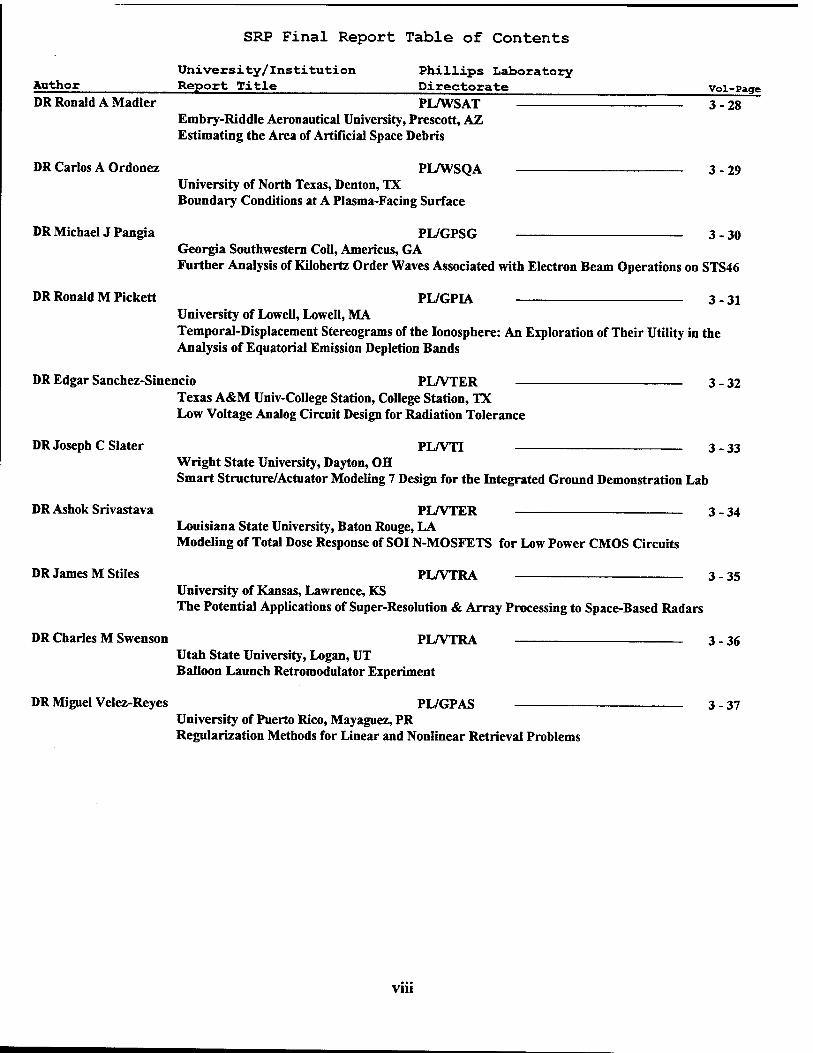
University/Institution Phillips Laboratory Author Report Title Directorate Voi-Page DR Ronald A Madler PL/WSAT 3-28

Embry-Riddle Aeronautical University, Prescott, AZ Estimating the Area of Artificial Space Debris

DR Carlos A Ordonez PLAVSQA 3-29 University of North Texas, Denton, TX Boundary Conditions at A Plasma-Facing Surface

DR Michael J Pangia PL/GPSG 3-30 Georgia Southwestern Coll, Americus, GA Further Analysis of Kilohertz Order Waves Associated with Electron Beam Operations on STS46

DR Ronald M Pickett PL/GPIA 3-31 University of Lowell, Lowell, MA Temporal-Displacement Stereograms of the Ionosphere: An Exploration of Their Utility in the Analysis of Equatorial Emission Depletion Bands

DR Edgar Sanchez-Sinencio PL/VTER 3-32 Texas A&M Univ-College Station, College Station, TX Low Voltage Analog Circuit Design for Radiation Tolerance

DR JosephC Slater PL/VTT 3-33 Wright State University, Dayton, OH Smart Structure/Actuator Modeling 7 Design for the Integrated Ground Demonstration Lab

DR Ashok Srivastava PL/VTER 3-34 Louisiana State University, Baton Rouge, LA Modeling of Total Dose Response of SOI N-MOSFETS for Low Power CMOS Circuits

DR James M Stiles PL/VTRA 3-35 University of Kansas, Lawrence, KS The Potential Applications of Super-Resolution & Array Processing to Space-Based Radars

DR Charles M Swenson PL/VTRA 3-36 Utah State University, Logan, UT Balloon Launch Retromodulator Experiment

DR Miguel Velez-Reyes PL/GPAS 3-37 University of Puerto Rico, Mayaguez, PR Regularization Methods for Linear and Nonlinear Retrieval Problems

VIII


University/Institution Rome Laboratory Author Report Title Directorate Voi-Page DRAFAnwar RL/ER 4-1

University of Connecticut, Storrs, CT A Study of Quantum Wells Formed in AlxGal-xAsySbl-y/InzGal-zAs/AlxGal-AsySbl-y Heterostructures

DR Ercument Arvas RL/OCSS 4-2 Syracuse University, Syracuse, NY An Assessment of the Current State of the Art of Stap from an Electromagnetics Point of View

DRAhmedEBarbour RL/ERDD 4-3 Georgia Southern University, Statesboro, GA Formal Verification Using ORA Larch/VEDL Theorem Prover

DRMilica Barjaktarovic RL/C3AB 4-4 Wilkes University, Wilkes Barre, PA Formal Specification and Verification of Missi Architecture Using Spin

DR Daniel C Bukofzer RL/C3BA 4-5 Cal State Univ, Fresno, Fresno, CA Performance Analysis & Simulation Results of Delay & Spread Spectrum Modulated Flip Wave-Signal Gene

DRXueshengChen RL/ERX 4-6 Wheaton College, Norton, MA Optical and Non-Destructive Methods to Determine the Composition and Thickness of an INxGAl-xAS/INP

DRJunChen RL/OCPA 4-7 Rochester Inst of Technology, Rochester, NY A Study of Optoelectronic Feedback-Sustained Pulsation of Laser Diodes at 1300 nm & 780 nm

DR Everett E Crisman RL/ERAC 4-8 Brown University, Providence, RI Evaluation of Semiconductor Configurations as Sources for Optically Induced Microwave Pulses

DRDigendraKDas RL/ERSR 4-9 SUNYIT, Utica, NY Techniques for Determining of the Precision of Reliability Predictions and Assessments.

DR Matthew E Edwards RL/ERDR 4-10 Spelman College, Atlanta, Ga The Analysis of PROFILER for Modeling the Diffusion of Aluminum-Copper on a Silicon Substrate

DR Kaliappan Gopalan RL/IRAA 4-11 Purdue University - Calumet, Hammond, IN Speaker Identification & Analysis of Stressed Speech

DR Joseph W Haus RL/OCPA 4-12 Rensselaer Polytechnic Institute, Troy, NY Mode-Locked Laser Models and Simulations

IX


Author University/Institution Report Title

Rone Laboratory Directorate

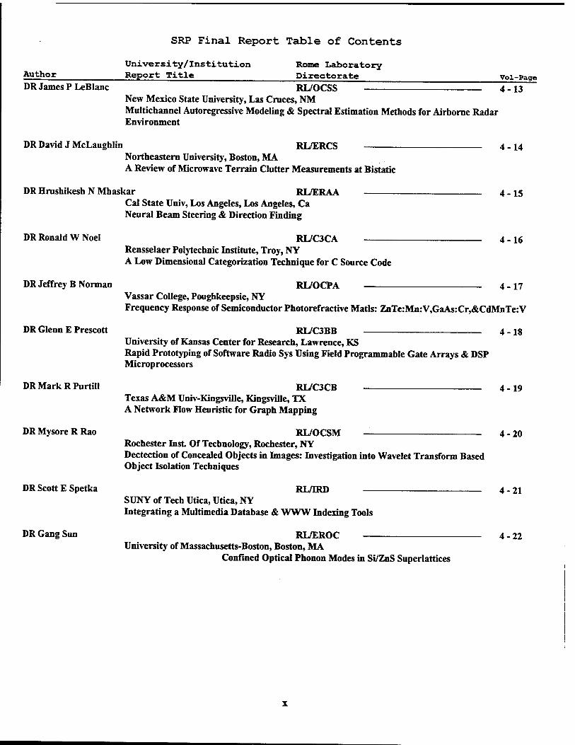
DR James P LeBlanc RL/OCSS New Mexico State University, Las Cruces, NM

Vol-Page

4-13

Multichannel Autoregressive Modeling & Spectral Estimation Methods for Airborne Radar Environment

DR David J McLaughlin RL/ERCS Northeastern University, Boston, MA A Review of Microwave Terrain Clutter Measurements at Bistatic

DR Hrushikesh N Mhaskar RL/ERAA Cal State Univ, Los Angeles, Los Angeles, Ca Neural Beam Steering & Direction Finding

DR Ronald W Noel RL/C3CA Rensselaer Polytechnic Institute, Troy, NY A Low Dimensional Categorization Technique for C Source Code

DR Jeffrey B Norman

DR Glenn E Prescott

RL/OCPA

4-14

4-15

4-16

4-17

DR Mark R Purtill

DR Mysore R Rao

DR Scott E Spetka

DR Gang Sun

Vassar College, Poughkeepsie, NY Frequency Response of Semiconductor Photorefractive Matls: ZnTe:Mn:V,GaAs:Cr,&CdMnTe:V

RL/C3BB University of Kansas Center for Research, Lawrence, KS Rapid Prototyping of Software Radio Sys Using Field Programmable Gate Arrays & DSP Microprocessors

RL/C3CB Texas A&M Univ-Kingsville, Kingsville, TX A Network Flow Heuristic for Graph Mapping

RL/OCSM Rochester Inst Of Technology, Rochester, NY Dectection of Concealed Objects in Images: Investigation into Wavelet Transform Based Object Isolation Techniques

RL/ERD SUNY of Tech Utica, Utica, NY Integrating a Multimedia Database & WWW Indexing Tools

4-18

4-19

4-20

RL/EROC University of Massachusetts-Boston, Boston, MA

4-21

4-22

Confined Optical Phonon Modes in Si/ZnS Superlattices


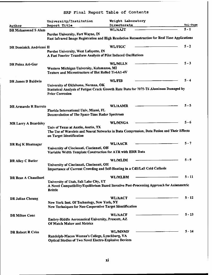
University/Institution Wright Laboratory Author Report Title Directorate voi-Page DRMohammad SAIam WL/AAJT 5-1

Purdue University, Fort Wayne, IN Fast Infrared Image Registration and High Resolution Reconstruction for Real Time Applications

DRDominickAndrisanin WL/FIGC 5-2 Purdue University, West Lafayette, IN A Fast Fourier Transform Analysis of Pilot Induced Oscillations

DRPninaAri-Gur WL/MLLN 5-3 Western Michigan University, Kalamazoo, MI Texture and Microstructure of Hot Rolled Ti-6A1-4V

DR James D Baldwin WL/FTB 5-4 University of Oklahoma, Norman, OK Statistical Analysis of Fatigue Crack Growth Rate Data for 7075-T6 Aluminum Damaged by Prior Corrosion

DR Armando RBarreto WL/AAMR 5-5 Florida International Univ, Miami, FL Deconvolution of The Space-Time Radar Spectrum

MR Larry A Beardsley WL/MNGA 5-6 Univ of Texas at Austin, Austin, TX The Use of Wavelets and Neural Networks in Data Compression, Data Fusion and Their Effects on Target Identification

DRRajKBhatnagar WL/AACR 5-7 University of Cincinnati, Cincinnati, OH Variable Width Template Construction for ATR with HRR Data

DR Alley C Butler WL/MLIM 5-9 University of Cincinnati, Cincinnati, OH Importance of Current Crowding and Self-Heating in a CdS/LaS Cold Cathode

DRReazAChaudhuri WL/MLBM 5-11 University of Utah, Salt Lake City, UT A Novel Compatibility/Equilibrium Based Iterative Post-Processing Approach for Arismmetric Brittle

DR Julian Cheung WL/AACT 5-12 New York Inst Of Technology, New York, NY New Techniques for Non-Cooperative Target Identification

DR Milton Cone WL/AACF 5-13 Embry-Riddle Aeronautical University, Prescott, AZ Of Match Maker and Metrics

DR Robert RCriss WL/MNMF 5-14 Randolph-Macon Woman's College, Lynchburg, VA Optical Studies of Two Novel Electro-Explosive Devices

XI


University/Institution Wright Laboratory Author Report Title Directorate voi-Page DR Robert J DeAngelis WL/MNM 5-15

Univ of Nebraska - Lincoln, Lincoln, NE Granin Size Effects in the Determination of X-Ray Pole figures and Orientation Distribution Function

DRYujieJDing WL/AADP 5-16 Bowling Green State University, Bowling Green, OH Investigation of Photoluminescence Intensity Saturation and Decay, and Nonlinear Optical Devices in Semiconductor Structures

DR Gregorys Elliott WL/POPT 5-17 Rutgers State Univ of New Jersey, Piscataway, NJ Laser Based Diagnostic Techniques for Combustion and Compressible Flows

DR Altan M Ferendeci WL/AADI 5-18 University of Cincinnati, Cincinnati, OH Vertical 3-D Interconnects for Multichip Modules

DR Dennis R Flentge WL/POSL 5-19 Cedarville College, Cedarville, OH Kinetic Studies of the Thermal Decomposition of Demnum and X-1P Using the System for Thermal Diagnostic Studies (STDS)

DR Himansu M Gajiwala WL/MLBP 5-20 Tuskegee University, Tuskegee, AL Novel Approach for the Compressive Strength Improvement of Rigid Rod Polymers

DR Allen G Greenwood WL/MTI 5-21 Mississippi State University, Mississippi State, MS A Framework for Manufacturing-Oriented, Design-Directed Cost Estimation

DR Rita A Gregory WL/FIVC 5-22 Georgia Inst of Technology, Atlanta, GA Affects of Int'l Quality Standards on Bare Base Waste Disposal Alternatives

DR Michael A Grinfeld WL/MLLM 5-23 Rutgers University, Piscataway, Piscataway, NJ Mismatch Stresses, Lamellar Microstructure & Mech

DRAwatef AHamed WL/FIM 5-24 University of Cincinnati, Cincinnati, OH Inlet Distortion Test Considerations for High Cycle Fatigue in Gas Turbine Engines

DR Stewart M Harris WL/MLPO 5-25 SUNY Stony Brook, Stony Brook, NY Compositional Modulation During Epitaxial Growth of Some IH-V Heterostructures

DR Larry S Heimick WL/MLBT 5-26 Cedarville College, Cedarville, OH Effect of Humidity on Wear of M-50 Steel with a Krytox Lubricant

DR Kenneth L Hensley MED/SGP 5-27 University of Oklahoma, Norman, OK Hyperbaric Oxygen Effects on the Postischemic Brain

xii



Wright Laboratory Directorate Vol-Page

DR Iqbal Husain

DR David W Johnson

WL/POOC university of Akron, Akron, OH Fault Analysis & Excitation Requirements for Switched Reluctance Starter-Generators

WL/MLBT

5-28

5-29 University of Dayton, Dayton, OH In Situ Formation of Standards for the Determination of Wear Metals in Perfluoropolyalkylether Lubricating Oils

DR Marian K Kazimierczuk WL/POOC Wright State University, Dayton, OH Aircraft Super Capacitor Back-Up System

DR Edward TKnobbe WL/MLBT Oklahoma State University, StUIwater, OK Corrosion Resistant Sol-Gel Coatings for Aircraft Aluminum Alloys

DR Michael C Larson WL/MLLM Tulane University, New Orleans, LA Cracks at Interfaces in Brittle Matrix Composites

DR Douglas A Lawrence WL/MNAG Ohio University, Athens, OH Analysis & Design of Gain Scheduled Missile Autopilots

DR Junghsen Lieh

DR Chun-Shin Lin

DR Zongli Lin

DRKuo-ChiLin

DR James S Marsh

WL/FTVM

5-30

5-31

5- 32

5-33

5-34

Wright State University, Dayton, OH Determination of 3D Deformations, Forces and Moments of Aircraft Tires with a Synchronized Optical and Analog System

WL/FIGP Univ of Missouri - Columbia, Columbia, MO Neural Network Technology for Pilot-Vehicle Interface & Decision Aids

WL/FI

5-35

5-36 SUNY Stony Brook, Stony Brook, NY Control of Linear Sys with Saturating Actuators with Applications to Flight Control Systems

WL/AASE University of Central Florida, Orlando, FL Study on Dead Reckoning Translation in High Level Architecture

WL/MNSI

5-37

5-38 University of West Florida, Pensacola, FL A Conceptual Model for Holographic Reconstruction & Minimizing Aberrations During Reconstruction

DR Paul Marshall WL/MLBT 5-39 University of North Texas, Denton, TX Computational Studies of the Reactions of CH3I With H and OH

XIII


University/Institution Wright Laboratory Author Report Title Directorate Voi-Page DRHuiMeng WL/POSC 5-40

Kansas State University, Manhattan, KS Investigation of Holographic PIV and Holographic Visualization techniques for Fluid Flows and Flames

DR Douglas J Miller WL/MLBP 5-41 Cedarville College, Cedarville, OH Band Gap Calculations on Oligomers with an All-Carbon Backbone

DR Ravi K Nadella WL/MLPO 5-42 Wilberforce University, Wilberforce, OH Hydrogen & Helium Ion Implantations for Obtaining High-Resistance Layers in N-Type 4H Silicon Carbide

DR Krishna Naishadham WL/MLPO 5-43 Wright State University, Dayton, OH Hydrogen & Helium Ion Implantations for Obtaining High-Resistance Layers in N-Type 4H Silicon

DR Timothy S Newman WL/AACR 5-44 Univ of Alabama at Huntsville, Huntsville, All A Summer Faculty Project for Anatomical Feature Extraction for Registration of Multiple Modalities of Brain MR

DR Mohammed Y Niamat WL/AAST 5-45 University of Toledo, Toledo, OH FPGA Implementation of the Xpatch Ray Tracer

DR James L Noyes WL/AACF 5-46 Wittenberg University, Springfield, OH The Development of New Learning Algorithms

DR Anthony COkafor WL/MTI 5-47 University of Missouri - Rolla, Rolla, MO Assessment of Developments in Machine Tool Technology

DRPaulDOrkwis WL/POPS 5-48 University of Cincinnati, Cincinnati, OH Assessing the Suitability of the CFD-H-Algorithm for Advanced Propulsion Concept simulations

Dr Robert PPenno WL/AAMP — 5-49 University of Dayton, Dayton, OH Grating Lobes in Antenna Arrays

DR George A Petersson WL/MLBT 5-50 Wesleyan University, Middletown, CT Absolute Rates for Chemical Reactions

DRMohamedNRahaman WL/MLLN 5-51 University of Missouri - Rolla, Rolla, MO

Effect of Solid Solution Additives on the Densification & Creep of Granular Ceramics

xrv



Wright Laboratory Directorate Vol-Page

DR Martin Schwartz WL/MLBT University of North Texas, Denton, TX AB Initio Modeling of the Enthalpies of Formation of Fluorocarbons

5-52

5-53 DR Thomas E Skinner MED/SGP Wright State University, Dayton, OH A Method for Studying Changes in Tissue Energetics Resulting from Hyperbaric Oxygen Therapy

DRMarekSkowronski WL/MLPO — 5-54 Carnegie Melon University, Pittsburgh, PA Investigation of Structural Defects in 4H-SiC Wafers

DR Grant D Smith WL/MLPJ Univ of Missouri - Columbia, Columbia, MO Theoretical Djvestigation of Phthalocyanin Dimers

DR James A Snide University of Dayton, Dayton, OH WL/MLLP Aging Aircraft: Preliminary Investigation of Various Materials and Process Issues

DR Yong D Song WL/MNAG North Carolina A & T State University, Greensboro, NC Memory-Base Control Methodology with Application to EMRAAT Missile

WL/MLIM DR Raghavan Srinivasan Wright State University, Dayton, OH Microstructural Development During Hot Deformation

DRJanuszAStarzyk WL/AACA Ohio University, Athens, OH Feature Selection for ATR Neural Network Approach

DR Alfred G Striz WL/FIB University of Oklahoma, Norman, OK On Multiobjective Function Optimization in Engineering Design

DR Barney E Taylor WL/MLBP Miami Univ - Hamilton, Hamilton, OH Optical and Electro-Optical Studies of Polymers

DR Joseph WTedesco WL/MNSA Auburn University, Auburn, AL Effects of Airblast Characteristics on Structural Response

DR Scott K Thomas

DR James P Thomas

DR Karen A Tomko

WL/POOS

5-55

5-56

5-57

5-58

5-59

5-60

5-61

5-62

5-63 Wright State University, Dayton, OH The Effects of Curvature on the Performance of a Spirally-Grooved Copper-Ethanol Heat Pipe

WL/MLLN University of Notre Dame, Notre Dame, IN Subcritical Crack Growth of Ti-6A1-4V Under Ripple Loading Conditions

WL/FTM

5-64

5-65 Wright State University, Dayton, OH Grid Level Parallelization of an Implicit Solution of the 3D Navier-Stokes Equations

xv



DR Saad A Ahmed AEDC King Fand Univ of Petroleum & Minerals, Saudi, Arabia

Arnold Engineering Development Center Directorate voi-Page

Turbulence Statistics & Energy Budget of a Turbulent Shear Layer

DR Csaba A Biegl AEDC Vanderbilt University, Nashville, TN Turbine Engine Blade Vibration Analysis System

DR Frank G Collins AEDC Tennessee Univ Space Institute, Tullahoma, TN Laser Vapor Screen Flow Visualization Technique

DR Randolph S Peterson AEDC The University of the South, Sewanee, TN

DR Robert L Roach AEDC Tennessee Univ Space Institute, Tullahoma, TN A Process for Setting Up Computation of Swirling Flows in the AEDC H-3 Heater

6-1

6-2

6-3

6-4

6-5

xvi


University/Institution U.S. Air Force Academy Author Report Title Directorate vol-Page DR Ryoichi Kawai USAFA 6-6

Univ of Alabama at Birmingham, Birmingham, AL A Massively Parallel Ab Initio Molecular Dynamis Simulation of Polymers & Molten Salts

xvii


University/Institution Air Logistic Centers Author Report Title Directorate Voi-Page DR Sandra A Ashford OCALC 6-7

University of Detroit Mercy, Detroit, MI Evaluation of Current Jet Engine Performance Parameters Archive, Retrieval and Diagnostic System

MR Jeffrey MBigelow OCALC 6-8 Oklahoma Christian Univ of Science & Art, Oklahoma City, OK Enhancing Tinker's Raster-to-Vector Capabilities

DR KM George OCALC 6-9 Oklahoma State University, Stillwater, OK A Computer Model for Sustainability Ranking

DRJagathJKaluarachichi OCALC 6-10 Utah State University, Logan, UT Optimal Groundwater Management Using Genetic Algorithm

XV1I1

INTRODUCTION

The Summer Research Program (SRP), sponsored by the Air Force Office of Scientific Research (AFOSR), offers paid opportunities for university faculty, graduate students, and high school students to conduct research in U.S. Air Force research laboratories nationwide during the summer.

Introduced by AFOSR in 1978, this innovative program is based on the concept of teaming academic researchers with Air Force scientists in the same disciplines using laboratory facilities and equipment not often available at associates' institutions.

The Summer Faculty Research Program (SFRP) is open annually to approximately 150 faculty members with at least two years of teaching and/or research experience in accredited U.S. colleges, universities, or technical institutions. SFRP associates must be either U.S. citizens or permanent residents.

Hie Graduate Student Research Program (GSRP) is open annually to approximately 100 graduate students holding a bachelor's or a master's degree; GSRP associates must be U.S. citizens enrolled full time at an accredited institution.

The High School Apprentice Program (HSAP) annually selects about 125 high school students located within a twenty mile commuting distance of participating Air Force laboratories.

AFOSR also offers its research associates an opportunity, under the Summer Research Extension Program (SREP), to continue their AFOSR-sponsored research at their home institutions through the award of research grants. In 1994 the maximum amount of each grant was increased from $20,000 to $25,000, and the number of AFOSR-sponsored grants decreased from 75 to 60. A separate annual report is compiled on the SREP.

The numbers of projected summer research participants in each of the three categories and SREP "grants" are usually increased through direct sponsorship by participating laboratories.

AFOSR's SRP has well served its objectives of building critical links between Air Force research laboratories and the academic community, opening avenues of communications and forging new research relationships between Air Force and academic technical experts in areas of national interest, and strengthening the nation's efforts to sustain careers in science and engineering. Tlie success of the SRP can be gauged from its growth from inception (see Table 1) and from the favorable responses the 1996 participants expressed in end-of-tour SRP evaluations (Appendix B).

AFOSR contracts for adrninistration of the SRP by civilian contractors. The contract was first awarded to Research & Development Laboratories (RDL) in September 1990. After

1

completion of the 1990 contract, RDL (in 1993) won the recompetition for the basic year and four 1-year options.

2. PARTICIPATION IN THE SUMMER RESEARCH PROGRAM

The SRP began with faculty associates in 1979; graduate students were added in 1982 and high school students in 1986. The following table shows the number of associates in the program each year.

YEAR SRP Participation, by Year ...

TOTAL

SFRP GSRP HSAP

1979 70 70

1980 87 87

1981 87 87 1982 91 17 108 1983 101 53 154 1984 152 84 236 1 1985 154 92 246 1 1986 158 100 42 300 1987 159 101 73 333 1988 153 107 101 361 1989 168 102 103 373 1990 165 121 132 418 1991 170 142 132 444 1992 185 121 159 464 1993 187 117 136 440 1994 192 117 133 442 1995 190 115 137 442 1996 188 109 138 435

Beginning in 1993, due to budget cuts, some of the laboratories weren't able to afford to fund as many associates as in previous years. Since then, the number of funded positions has remained fairly constant at a slightly lower level.

3. RECRUITING AND SELECTION

The SRP is conducted on a nationally advertised and competitive-selection basis. The advertising for faculty and graduate students consisted primarily of the mailing of 8,000 52- page SRP brochures to chairpersons of departments relevant to AFOSR research and to administrators of grants in accredited universities, colleges, and technical institutions. Historically Black Colleges and Universities (HBCUs) and Minority Institutions (Mis) were included. Brochures also went to all participating USAF laboratories, the previous year's participants, and numerous individual requesters (over 1000 annually).

RDL placed advertisements in the following publications: Black Issues in Higher Education, Winds of Change, and TF.F.K Spectrum. Because no participants list either Physics Today or Chemical & Engineering News as being their source of learning about the program for the past several years, advertisements in these magazines were dropped, and the funds were used to cover increases in brochure printing costs.

High school applicants can participate only in laboratories located no more than 20 miles from their residence. Tailored brochures on the HSAP were sent to the head counselors of 180 high schools in the vicinity of participating laboratories, with instructions for publicizing the program in their schools. High school students selected to serve at Wright Laboratory's Armament Directorate (Eglin Air Force Base, Florida) serve eleven weeks as opposed to the eight weeks normally worked by high school students at all other participating laboratories.

Each SFRP or GSRP applicant is given a first, second, and third choice of laboratory. High school students who have more than one laboratory or directorate near their homes are also given first, second, and third choices.

Laboratories make their selections and prioritize their nominees. AFOSR then determines the number to be funded at each laboratory and approves laboratories1 selections.

Subsequently, laboratories use their own funds to sponsor additional candidates. Some selectees do not accept the appointment, so alternate candidates are chosen. This multi-step selection procedure results in some candidates being notified of their acceptance after scheduled deadlines. The total applicants and participants for 1996 are shown in this table.

1996 Applicants and Participants

PARTICIPANT CATEGORY

TOTAL APPLICANTS

SELECTEES DECLINING SELECTEES

SFRP 572 188 39

(HBCU/MI) (119) (27) (5) GSRP 235 109 7

(HBCU/MI) (18) (7) (1)

HSAP 474 138 8

TOTAL 1281 435 54

4. SITE VISITS

During June and July of 1996, representatives of both AFOSR/NI and RDL visited each participating laboratory to provide briefings, answer questions, and resolve problems for both laboratory personnel and participants. The objective was to ensure that the SRP would be as constructive as possible for all participants. Both SRP participants and RDL representatives found these visits beneficial. At many of the laboratories, this was the only opportunity for all participants to meet at one time to share their experiences and exchange ideas.

5. HISTORICALLY BLACK COLLEGES AND UNIVERSITIES AND MINORITY INSTITUTIONS (HBCU/Mb)

Before 1993, an RDL program representative visited from seven to ten different HBCU/Mis annually to promote interest in the SRP among the faculty and graduate students. These efforts were marginally effective, yielding a doubling of HBCI/MI applicants. In an effort to achieve AFOSR's goal of 10% of all applicants and selectees being HBCU/MI qualified, the RDL team decided to try other avenues of approach to increase the number of qualified applicants. Through the combined efforts of the AFOSR Program Office at Boiling AFB and RDL, two very active minority groups were found, HACU (Hispanic American Colleges and Universities) and AISES (American Indian Science and Engineering Society). RDL is in communication with representatives of each of these organizations on a monthly basis to keep up with the their activities and special events. Both organizations have widely-distributed magazines/quarterlies in which RDL placed ads.

Since 1994 the number of both SFRP and GSRP HBCU/MI applicants and participants has increased ten-fold, from about two dozen SFRP applicants and a half dozen selectees to over 100 applicants and two dozen selectees, and a half-dozen GSRP applicants and two or three selectees to 18 applicants and 7 or 8 selectees. Since 1993, the SFRP had a two-fold applicant

4

increase and a two-fold selectee increase. Since 1993, the GSRP had a three-fold applicant increase and a three to four-fold increase in selectees.

In addition to RDL's special recruiting efforts, AFOSR attempts each year to obtain additional funding or use leftover funding from cancellations the past year to fund HBCU/MI associates. This year 5 HBCU/MI SFRPs declined after they were selected (and there was no one qualified to replace them with). The following table records HBCU/MI participation in this program.

SRP HBCU/MI Participation, By Year

YEAR SFRP GSRP

Applicants Participants Applicants Participants

1985 76 23 15 11

1986 70 18 20 10

1987 82 32 32 10

1988 53 17 23 14

1989 39 15 13 4

1990 43 14 17 3

1991 42 13 8 5

1992 70 13 9 5

1993 60 13 6 2

1994 90 16 11 6

1995 90 21 20 8

1996 119 27 18 - 7

6. SRP FUNDING SOURCES

Funding sources for the 1996 SRP were the AFOSR-provided slots for the basic contract and laboratory funds. Funding sources by category for the 1996 SRP selected participants are shown here.

1996 SRP FUNDING CATEGORY SFRP GSRP HSAP

AFOSR Basic Allocation Funds 141 85 123

USAF Laboratory Funds 37 19 15

HBCU/MI By AFOSR (Using Procured Addn'l Funds)

10 5 0

TOTAL 188 109 138

SFRP -150 were selected, but nine canceled too late to be replaced. GSRP - 90 were selected, but five canceled too late to be replaced (10 allocations for the ALCs were withheld by AFOSR) HSAP -125 were selected, but two canceled too late to be replaced.

COMPENSATION FOR PARTICIPANTS

Compensation for SRP participants, per five-day work week, is shown in this table.

1996 SRP Associate Compensation

PARTICIPANT CATEGORY 1991 1992 1993 1994 1995 1996

Faculty Members $690 $718 $740 $740 $740 $770

Graduate Student (Master's Degree)

$425 $442 $455 $455 $455 $470

Graduate Student (Bachelor's Degree)

$365 $380 $391 $391 $391 $400

High School Student (First Year)

$200 $200 $200 $200 $200 $200 1

High School Student (Subsequent Years)

$240 $240 $240 $240 $240 $240 1

The program also offered associates whose homes were more than 50 miles from the laboratory an expense allowance (seven days per week) of $50/day for faculty and $40/day for graduate students. Transportation to the laboratory at the beginning of their tour and back to their home destinations at the end was also reimbursed for these participants. Of the combined SFRP and

GSRP associates, 65 % (194 out of 297) claimed travel reimbursements at an average round- trip cost of $780.

Faculty members were encouraged to visit their laboratories before their summer tour began. All costs of these orientation visits were reimbursed. Forty-five percent (85 out of 188) of faculty associates took orientation trips at an average cost of $444. By contrast, in 1993, 58 % of SFRP associates took orientation visits at an average cost of $685; that was the highest percentage of associates opting to take an orientation trip since RDL has administered the SRP, and the highest average cost of an orientation trip. These 1993 numbers are included to show the fluctuation which can occur in these numbers for planning purposes.

Program participants submitted biweekly vouchers countersigned by their laboratory research focal point, and RDL issued paychecks so as to arrive in associates' hands two weeks later.

In 1996, RDL implemented direct deposit as a payment option for SFRP and GSRP associates. There were some growing pains. Of the 128 associates who opted for direct deposit, 17 did not check to ensure that their financial institutions could support direct deposit (and they couldn't), and eight associates never did provide RDL with their banks' ABA number (direct deposit bank routing number), so only 103 associates actually participated in the direct deposit program. The remaining associates received their stipend and expense payments via checks sent in the US mail.

HSAP program participants were considered actual RDL employees, and their respective state and federal income tax and Social Security were withheld from their paychecks. By the nature of their independent research, SFRP and GSRP program participants were considered to be consultants or independent contractors. As such, SFRP and GSRP associates were responsible for their own income taxes, Social Security, and insurance.

8. CONTENTS OF THE 1996 REPORT

The complete set of reports for the 1996 SRP includes this program management report (Volume 1) augmented by fifteen volumes of final research reports by the 1996 associates, as indicated below:

1996 SRP Final Report Volume Assignments

LABORATORY SFRP GSRP HSAP

Armstrong 2 7 12

Phillips 3 8 13

Rome 4 9 14

Wright 5A,5B 10 15

AEDC, ALCs, WHMC 6 11 16

APPENDIX A - PROGRAM STATISTICAL SUMMARY

A. Colleges/Universities Represented

Selected SFRP associates represented 169 different colleges, universities, and institutions, GSRP associates represented 95 different colleges, universities, and institutions.

B. States Represented

SFRP -Applicants came from 47 states plus Washington D.C. and Puerto Rico. Selectees represent 44 states plus Puerto Rico.

GSRP - Applicants came from 44 states and Puerto Rico. Selectees represent 32 states.

HSAP - Applicants came from thirteen states. Selectees represent nine states.

Total Number of Participants

SFRP 188

GSRP 109

HSAP 138

TOTAL 435

Degrees Represented

SFRP GSRP TOTAL

Doctoral 184 1 185

Master's 4 48 52

Bachelor's 0 60 60

TOTAL 188 109 297 |

A-l

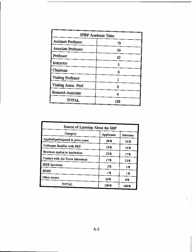
Source of Learning About the SRP

Categoiy

Applied/participated in prior years

Colleague familiar with SRP

Brochure mailed to institution

Contact with Air Force laboratory

IEEE Spectrum

BIIHE

Other source

TOTAL

Applicants

28%

19%

23%

17%

2%

1%

10%

100%

Selectees

34%

16%

17%

23%

8%

100%

A-2

APPENDIX B - SRP EVALUATION RESPONSES

1. OVERVIEW

Evaluations were completed and returned to RDL by four groups at the completion of the SRP. The number of respondents in each group is shown below.

Table B-l. Total SRP Evaluations Received

Evaluation Group Responses

SFRP & GSRPs 275

HSAPs 113

USAF Laboratory Focal Points 84

USAF Laboratory HSAP Mentors 6

All groups indicate unanimous enthusiasm for the SRP experience.

The summarized recommendations for program improvement from both associates and laboratory personnel are listed below:

A. Better preparation on the labs' part prior to associates' arrival (i.e., office space, computer assets, clearly defined scope of work).

B. Faculty Associates suggest higher stipends for SFRP associates.

C. Both HSAP Air Force laboratory mentors and associates would like the summer tour extended from the current 8 weeks to either 10 or 11 weeks; the groups state it takes 4-6 weeks just to get high school students up-to-speed on what's going on at laboratory. (Note: this same argument was used to raise the faculty and graduate student participation time a few years ago.)

B-l

2. 1996 USAF LABORATORY FOCAL POINT (LFP) EVALUATION RESPONSES

The summarized results listed below are from the 84 LFP evaluations received.

1. LFP evaluations received and associate preferences:

Table B-2. Air Force LFP Evaluation Responses (By Type)

Lab

AEDC WHMC AL FJSRL PL RL WL Total

Evals Recv'd

0 0 7 1

25 5

46

How Many Associates Would You Prefer To Get? (% Response) SFRP

1 2 3+

84

28 0 40 60 30

28 100 40 40 43

28 0 16 0 20

14 0 4 0 6

32% 50% 13% 5%

GSRP (w/Univ Professor) 3+

54 100 88 80 78

14 0 12 10 17

28 0 0 0 4

0 0 0 0 0

GSRP (w/o Univ Professor) 0 12 3+

80% 11% 6% 0%

86 0 84 100 93

0 100 12 0 4

14 0 4 0 2

0 0 0 0 0

73% 23% 4% 0%

LFP Evaluation Summary. The summarized responses, by laboratory, are listed on the following page. LFPs were asked to rate the following questions on a scale from 1 (below average) to 5 (above average).

2. Lros involved in SRP associate appücation evaluation process: a. Time available for evaluation of applications: b. Adequacy of applications for selection process:

3. Value of orientation trips: 4. Length of research tour 5 a. Benefits of associate's work to laboratory:

b. Benefits of associate's work to Air Force: 6. a. Enhancement of research qualifications for LFP and staff:

b. Enhancement of research qualifications for SFRP associate: c. Enhancement of research qualifications for GSRP associate:

7. a. Enhancement of knowledge for LFP and staff: b. Enhancement of knowledge for SFRP associate: c. Enhancement of knowledge for GSRP associate:

Value of Air Force and university links: Potential for future collaboration:

a. Your woriring relationship with SFRP: b. Your working relationship with GSRP:

11. Expenditure of your time worthwhile: (Continued on next page)

8. 9. 10

B-2

12. Quality of program literature for associate: 13. a. Quality of RDL's communications with you:

b. Quality of RDL's communications with associates: 14. Overall assessment of SRP:

Table] B-3. Laboratory Focal Point Reponses to above questions AEDC AL FJSRL PL RL WHMC WL

MEvalsRecv'd 0 7 1 14 5 0 46 Question it

2 - 86% 0% 88 % 80% - 85 % 2a - 4.3 n/a 3.8 4.0 - 3.6 2b - 4.0 n/a 3.9 4.5 - 4.1 3 - 4.5 n/a 4.3 4.3 - 3.7 4 - 4.1 4.0 4.1 4.2 - 3.9 5a - 4.3 5.0 4.3 4.6 - 4.4 5b - 4.5 n/a 4.2 4.6 - 4.3 6a - 4.5 5.0 4.0 4.4 - 4.3 6b - 4.3 n/a 4.1 5.0 - 4.4 6c - 3.7 5.0 3.5 5.0 - 4.3 7a - 4.7 5.0 4.0 4.4 - 4.3 7b - 4.3 n/a 4.2 5.0 - 4.4 7c - 4.0 5.0 3.9 5.0 - 4.3 8 - 4.6 4.0 4.5 4.6 - 4.3 9 - 4.9 5.0 4.4 4.8 - 4.2

10a - 5.0 n/a 4.6 4.6 - 4.6 10b - 4.7 5.0 3.9 5.0 - 4.4 11 - 4.6 5.0 4.4 4.8 - 4.4 12 - 4.0 4.0 4.0 4.2 - 3.8 13a - 3.2 4.0 3.5 3.8 - 3.4 13b - 3.4 4.0 3.6 4.5 - 3.6 14 - 4.4 5.0 4.4 4.8 - 4.4

B-3

3. 1996 SERP&GSRP EVALUATION RESPONSES

The summarized results listed below are from the 257 SFRP/GSRP evaluations received.

Associates were asked to rate the following questions on a scale from 1 (below average) to 5 (above average) - by Air Force base results and over-all results of the 1996 evaluations are listed after the questions.

1. The match between the laboratories research and your field: 2. Your working relationship with your LFP: 3. Enhancement of your academic qualifications: 4. Enhancement of your research qualifications: 5. Lab readiness for you: LFP, task, plan: 6. Lab readiness for you: equipment, supplies, facilities: 7. Lab resources: 8. Lab research and administrative support: 9. Adequacy of brochure and associate handbook: 10. RDL communications with you: 11. Overall payment procedures: 12. Overall assessment of the SRP: 13. a. Would you apply again?

b. Will you continue this or related research? 14. Was length of your tour satisfactory? 15. Percentage of associates who experienced difficulties in finding housing: 16. Where did you stay during your SRP tour?

a. At Home: b. With Friend: c. On Local Economy: d. Base Quarters:

17. Value of orientation visit: a. Essential: b. Convenient: c. Not Worth Cost: d. Not Used:

SFRP and GSRP associate's responses are listed in tabular format on the following page.

B-4

Table B-4. 1996 SFRP & GSRP Associate Responses to SRP Evaluation

Arnold Brooks Edwards Egfin Griffe Hanmm KeDy Kbtbnd Lackland Robins Tyndall WPAFB ««t»

res 6 48 6 14 31 19 3 32 1 2 10 85 257

1 4.8 4.4 4.6 4.7 4.4 4.9 4.6 4.6 5.0 5.0 4.0 4.7 4.6 2 5.0 4.6 4.1 4.9 4.7 4.7 5.0 4.7 5.0 5.0 4.6 4.8 4.7 3 4.5 4.4 4.0 4.6 4.3 4.2 4.3 4.4 5.0 5.0 4.5 4.3 4.4 4 4.3 4.5 3.8 4.6 4.4 4.4 4.3 4.6 5.0 4.0 4.4 4.5 4.5 5 4.5 4.3 3.3 4.8 4.4 4.5 4.3 4.2 5.0 5.0 3.9 4.4 4.4 6 4.3 4.3 3.7 4.7 4.4 4.5 4.0 3.8 5.0 5.0 3.8 4.2 42 7 4.5 4.4 4.2 4.8 4.5 4.3 4.3 4.1 5.0 5.0 4.3 43 4.4 8 4.5 4.6 3.0 4.9 4.4 4.3 4.3 4.5 5.0 5.0 4.7 4.5 4.5 9 4.7 4.5 4.7 4.5 4.3 4.5 4.7 4J 5.0 5.0 4.1 4.5 4.5 10 4.2 4.4 4.7 4.4 4.1 4.1 4.0 42 5.0 4.5 3.6 4.4 43 11 3.8 4.1 4.5 4.0 3.9 4.1 4.0 4.0 3.0 4.0 3.7 4.0 4.0 12 5.7 4.7 43 4.9 4.5 4.9 4.7 4.6 5.0 4.5 4.6 4.5 4.6

Numbers below are percentages 13a 83 90 83 93 87 75 100 81 100 100 100 86 87 13b 100 89 83 100 94 98 100 94 100 100 100 94 93 14 83 96 100 90 87 80 100 92 100 100 70 84 88 15 17 6 0 33 20 76 33 25 0 100 20 8 39 16a . 26 17 9 38 23 33 4 - - - 30 16b 100 33 • 40 . 8 - - - - 36 2 16c 41 83 40 62 69 67 96 100 100 64 68 16d «. . _ . . - - - - - - 0 17a _ 33 100 17 50 14 67 39 - 50 40 31 35 17b _ 21 . 17 10 14 - 24 - 50 20 16 16 17c . . . . 10 7 - - - - - 2 3 17d 100 46 - 66 30 69 33 37 100 - 40 51 46

B-5

4. 1996 USAF LABORATORY HSAP MENTOR EVALUATION RESPONSES

Not enough evaluations received (5 total) from Mentors to do useful summary.

B-6

5. 1996 HSAP EVALUATION RESPONSES

The summarized results listed below are from the 113 HSAP evaluations received.

HSAP apprentices were asked to rate the following questions on a scale from 1 (below average) to 5 (above average)

1. Your influence on selection of topic/type of work. 2. Working relationship with mentor, other lab scientists. 3. Enhancement of your academic qualifications. 4. Technically challenging work. 5. Lab readiness for you: mentor, task, work plan, equipment. 6. Influence on your career. 7. Increased interest in math/science. 8. Lab research & administrative support. 9. Adequacy of RDL's Apprentice Handbook and administrative materials. 10. Responsiveness of RDL communications. 11. Overall payment procedures. 12. Overall assessment of SRP value to you. 13. Would you apply again next year? Yes (92 %) 14. Will you pursue future studies related to this research? Yes (68 %) 15. Was Tour length satisfactory? Yes (82 %)

Arnold Brooks Edwards EgHn Griffiss Hanscom Kirdand Tyndafl WPAFB Totals #

icsp 5 19 7 15 13 2 7 5 40 113

1 2

2.8 4.4

3.3 4.6

3.4 4.5

3.5 4.8

3.4 4.6

4.0 4.0

3.2 4.4

3.6 4.0

3.6 4.6

3.4 4.6

3 4

4.0 3.6

4.2 3.9

4.1 4.0

4.3 4.5

4.5 4.2

5.0 5.0

4.3 4.6

4.6 3.8

4.4 4.3

4.4 4.2

5 6

4.4 3.2

4.1 3.6

3.7 3.6

4.5 4.1

4.1 3.8

3.0 5.0

3.9 3.3

3.6 3.8

3.9 3.6

4.0 3.7

7 8

2.8 3.8

4.1 4.1

4.0 4.0

3.9 4.3

3.9 4.0

5.0 4.0

3.6 4.3

4.0 3.8

4.0 4.3

3.9 4.2

9 10

4.4 4.0

3.6 3.8

4.1 4.1

4.1 3.7

3.5 4.1

4.0 4.0

3.9 3.9

4.0 2.4

3.7 3.8

3.8 3.8

11 12

4.2 4.0

4.2 4.5

3.7 4.9

3.9 4.6

3.8 4.6

3.0 5.0

3.7 4.6

2.6 4.2

3.7 4.3

3.8 4.5

Numbers below are percenta ges 13 14

60% 20%

95% 80%

100% 71%

100% 80%

85% 54%

100% 100%

100% 71%

100% 80%

90% 65%

92% 68%

15 100% 70% 71% 100% 100% 50% 86% 60% 80% 82%

B-7

Fast Infrared Image Registration and High Resolution Reconstruction for Real Time Applications

Mohammad S. Alam Assistant Professor of Electrical Engineering

Purdue University, ET 327A, Fort Wayne, IN 46805-1499 (219)481 -6020, [email protected]

Final Project Report: Summer Faculty Research Program

Air Force Wright Laboratory, Dayton, Ohio

Sponsored by: Air Force Office of Scientific Research

Boiling Air Force Base, DC and

Wright Laboratory, Wright-Patterson Air Force Base, Ohio

August 1996

1-1

Abstract

Forward looking infrared (FLIR) detector arrays generally produce low resolution images because the FLIR arrays can not be made sufficiently dense to yield a high sampling frequency using the current technology. Microscanning is an effective technique for reducing aliasing and increasing resolution in images produced by staring infrared imaging systems, which involves recording a sequence of frames through subpixel movements of the field of view on the detector array and then interlacing them to produce a high resolution image. The FLIR system is usually mounted on a moving platform, such as an aircraft, and the normal vibrations associated with the moving platform can be used to generate shifts in the FLIR recorded sequence of frames. Since a fixed number of frames is required for a given level of microscanning, and the shifts are random, some of the acquired frames may have almost similar shifts thus making them unusable for high resolution image reconstruction. In this paper, we utilize a modified version of the algorithm reported in Ref. 1 for estimating the shifts among the acquired frames and then utilize a it- nearest-neighbor approach for estimating the above mentioned missing frames to form the final high resolution image. Blurring by the detector and optics of the imaging system limits the increase in image resolution when microscanning is attempted at sub-pixel movements of less than half the detector width. We resolve this difficulty by the application of Wiener filter, designed using the MTF of the imaging system, to the microscanned images. Computer simulation and experimental results are presented to verify the effectiveness of the proposed technique. This technique is significantly faster than the alternate techniques, and is found to be especially suitable for real time applications.

1-2

1 Introduction

In many Forward Looking Infrared (FLIR) imaging systems, the detector spacing in the focal plane array is not sufficiently small so as to sample a band-limited scene at the Nyquist rate, resulting in a degraded image due to aliasing artifacts. The construction of a focal plane array with smaller and more closely spaced detector elements is very difficult and prohibitively expensive due to fabrication complexity and quantum efficiency problems. Over the last four years, the Electro-Optics Branch of Wright Laboratory has been developing a microscan imaging technique to increase the spatial sampling rate of existing focal plane arrays and to alleviate the aliasing effects in infrared imagery2. The microscanning process uses a sequence of spatially undersampled time frames of a scene to generate the high resolution image. Each frame is subpixel shifted relative to each other frame onto a set grid pattern. The sequence of frames are then interlaced to yield the high resolution image which represents the input scene effectively sampled at a higher spatial frequency. The aforementioned process is called controlled microscanning because the subpixel shifts between the temporal image frames are controlled and therefore known a priori. In this paper, we consider a practical scenario where an imager is mounted on a moving and/or vibrating platform, such as an aircraft. Consequently, controlled microscanning can not be used for such applications. Uncontrolled microscanning is the process where the shifts for each frame are unknown and must be estimated before registering onto the high resolution grid pattern. The shifts for each frame are unknown because they are generated by the random motion and/or vibration of the imager platform and not by a microscan mirror. Using random shifts alone eliminates the necessity for a microscan mirror and driver system. Since a fixed number of frames is required for a given level of microscanning, and the shifts are random, some of the acquired frames may have almost similar shifts which will create empty bins in the high resolution image reconstruction. Thus, the key factors for the high resolution image reconstruction are the accurate knowledge of the subpixel translational motion of the scene relative to the FLIR array and the accurate estimation of the missing frames (a frame whose translational shifts are similar to another frame or a frame which does not exist corresponding to a desired grid pattern). In this paper, we have utilized a modified version of the algorithm reported in Ref. 1 for estimating the shifts between the acquired frames and then used a k- nearest-neighbor approach for estimating the aforementioned missing frames. The proposed algorithm is significantly faster than alternate techniques3,4 and is found to be suitable for real time applications.

With the increase of microscan level (i.e., smaller and smaller subpixel movements), we expect to see a proportional increase in resolution of the final reconstructed image. However, attempts at increasing the resolution beyond the Nyquist rate produce images having the same general appearance independent of microscan level. This bottleneck in the microscanning process was found to be primarily caused by the blurring inherent to the system's modulation transfer function (MTF). The main contributors to the system MTF are the optical transfer function and the detector transfer function. Since all parameters of the imager optics and detector array are known, it is possible to accurately model the system MTF. The application of a Wiener filter was found to be an effective means of removing the blurring caused by the system MTF and improving the resolution of microscanned image data. Computer simulations were performed by varying the level of microscanning along with the optical transfer function and detector transfer function. The resulting images are then compared with those images produced after using Wiener

1-3

filtering to deconvolve the optical and detector blurring functions out of the microscan images. Note that the Wiener filter restoration is done in the discrete domain on the sensor's discrete output image. However, the blurring of an image by the optics and detectors of the sensor is a continuous process. Therefore the continuous blurring function must be mapped to a discrete blurring function to be used to create a discrete Wiener filter for restoration. To avoid aliasing in the continuous to discrete conversion of the function, the continuous function must be sampled at a high enough frequency so as to meet the Nyquist rate. Microscanning increases this sampling rate and allows the continuous functions to be properly mapped and used to form the discrete Wiener filter for restoration.

A considerable understanding of the advantages and limitation of the Wiener filtering technique was acquired from the information compiled during the microscan simulation. The knowledge acquired from the simulation was applied to restoring imagery collected from a real-time FLIR imaging system. From the simulation and experimental results, it is evident that the proposed k- nearest-neighbor approach for estimating the missing frames significantly improves the image quality. The resolution of the final high resolution image can be improved further by the application of Wiener filtering, especially for alleviating the effects of blurring caused by system MTF.

2 The Sampling Process

2.1 Sampling in a FLIR Array

In a FLIR array, sampling is performed by a finite sized array of detectors and three main factors must be taken into consideration: the optical point spread function, the detector charge integration, and the detector array geometry. The block diagram in Fig. 1 illustrates the sampling process in a FLIR array. The object scene, denoted o(x,y), is convolved with the point spread function of the optics, psf(x,y), and the aperture function for the square detector6, d(x,y).

Point Spread Function

Detector Integration nXy) samp(x,y)

Finite Detector Sampling Array Function

Figure 1. Block diagram of the imaging system.

For our imaging system, we assume the detector has a flat response across its active region so the detector function can be expressed as:

1 (x y\ d(x,y) = j—rrect - — , (1)

\ab\ \a bj where a and b are the dimensions of the individual detectors. The result is multiplied by a function representing the limited extent of the detector array, r(x,y), expressed as

1-4

r(x,y) = rect\ (2)

where X and Y are the dimensions of the array. To apply this integration to all of the detectors, it is multiplied by the sampling lattice, combA^AyCxj),

comb^U,y) =— 1 Z_S[J; -m. £-» j = 1 lj (x-**.y-*iy) (3)

where Ax and Ay are the center-to-center detector spacings. The resulting expression for the staring image is

Kx, y) = o(x,y)*Psf(x,y>^rect^ rect x y ,- • comVA>(*>>>)• X Y

(4)

An illustration of a uniform detector array showing critical dimensions is shown in Fig. 2.

ÄX ■ ■ ■ ■

m-M * Active

Area

■ ■ ■

1 ■ 1 1 Figure 2. The detector array.

2.2 Controlled Microscanning

In controlled microscanning, the subpixel shifts between temporal image frames are controlled and therefore known in advance. A level L microscan is defined to be the case where L staring frames are acquired for each high resolution frame and each staring frame has its own unique controlled subpixel shift, each shift being part of a uniform grid. Thus, each staring frame has a shift that is integer multiple of 1/L times the detector width. The staring frames are interlaced in an LxL pattern to produce a high resolution frame of size NLxNL where N is the size of the square detector array. For a level 2 or 2x2 microscanned image, the original scene is stepped one half the length of the detector in the x and y directions producing a series of four staring images. These images are then interlaced to produce the resulting microscan image of 2Nx2N pixels, as shown in Fig. 3 where the reconstructed image has 4 times the number of unique samples as any of the four frames. Thus, a level-L microscanning effectively increases the sampling frequency by L without changing the detector size or spacing. Since the effect of the finite detector array

1-5

r(x,y) is small compared to the effects of the detector integration and the psf, neglecting the effect of r(x,y), an LxL microscan process can be expressed as

1 -kl! -kJ f i i\ i(x,y)= o(x,y)*psf(x,y)*7J-rrect\-, Y 1 (x y)

.—rrect\ —,— . y, . \ab\ \a b)\L i=0 j=Q

1-1 l-l f j j

(5)

where the factor of 1/L2 is used to adjust for the reduction in detector integration time at each of the L2 microscan steps.

+ +». + +

+ ®^ + +

Frame 1

^ + + +

Frame 2

+ +M + /*

+ + + +

+ J + +^ +

+ + + +

Frame 4 Frame 3

Detector Size 1

+ 2

+ i 2

+ —I + 2 +

1 +

2 +

4 +

3 a 4 + 4 'Z ̂ 3

*^S /T. A/ 1

+ 2

+ 4

+ 3 a

+ + ^ 4 &

+

+ S^n* *+ + 4

+ + „ 4

+ 3

+ 4 3

+ + 4

+ 3

+

Microscan Pattern

Figure 3. Illustration of a level 2 microscanning process.

2.3 Uncontrolled Microscanning

Uncontrolled microscanning results from practical applications where the imager is mounted on a moving and/or vibrating platform, such as an aircraft, and the vibrations associated with the platform can be exploited to create the shifts in the acquired frames. In uncontrolled microscanning, the shifts for each recorded frame are unknown and must be obtained before forming an estimate of the high resolution image. Because the shifts are random in uncontrolled microscanning, it eliminates the need for a microscan mirror and driver system otherwise required in controlled microscanning. Since a fixed number of frames is required for a given level of microscanning, and the shifts are random, some of the acquired frames may have almost similar shifts or unusable shifts which will generate empty bins in the high resolution image reconstruction. Thus, the key factors for the high resolution image reconstruction are the accurate knowledge of the subpixel translational motion of the scene relative to the FLIR array and the accurate estimation of the missing frames for filling the empty bins in the high resolution image.

1-6

3 Image Registration

For uncontrolled microscanning, the movement of the scene on the array is produced by random motion and/or vibration of the imager platform. Therefore the image shifts are unknown for each recoreded frame. It is necessary to develop a suitable algorithm which can accurately estimate the registration parameters i.e., in our case, the random translational shifts. Various algorithms have been reported in the literature for estimating the image registration parameters •' . Among these techniques, the gradient based registration technique proposed in Ref. 2 appears to be particularly attractive for practical applications. However, this technique only works for small shifts. To accommodate the case where larger shift values are anticipated, we utilized the iterative technique proposed in Ref. 7 and incorporated it with the registration algorithm proposed in Ref. 1. In this algorithm, the first acquired frame is considered to be the reference frame and the shifts associated with the remaining frames are calculated with respect to the reference frame. If p represents the total number of frames acquired by the imager, and hk and vk represents the shifts in the horizontal and vertical directions for the fcth frame, then the observed Mi frame may be expressed as

ok(x,y)=ol(x + hk,y + vk), (6)

where k e (2, 3, 4, ..., p} and for the reference frame, hi = v; = 0. Considering the first three terms for the Taylor series expansion, Eq. (6) may be approximated as

ok(x,y) ~ol(x,y) + hk

dox{x,y) dox{x,y) ■ + v (7)

dx ' 'k dy '

Since Eq. (7) is an approximation itself and discrete estimates of x and y must be used, it is useful to apply the method of least squares for solving the registration parameters hk and v*. For the least squares solution9 the error expression

Ek(hk,vk) « 1

MN

M N

II m=\ n = l

ok(m,n)-ol(m,n) -hk

(9o,(m,n) dox(m,n) --v (8)

dm '* dn

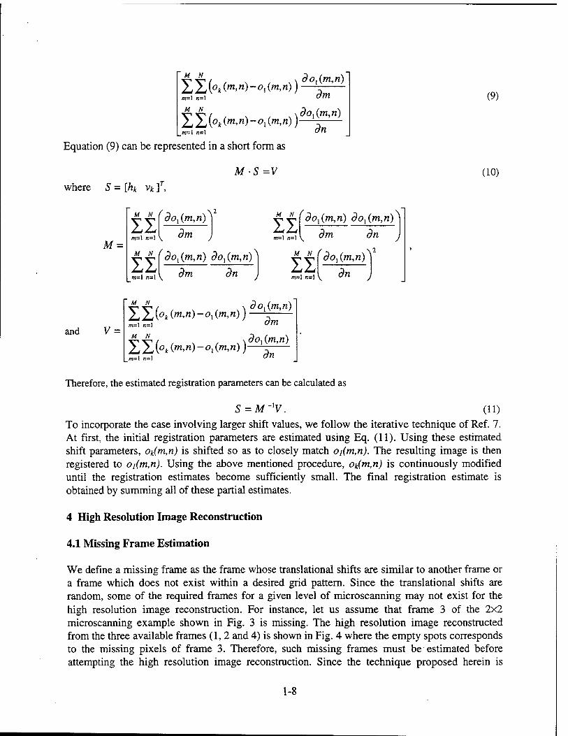
must be minimized, where m and n are discrete variables for the x and y directions, M and N represents the total number of pixels in the x and y directions, and hk and v* are the translational shifts in the x and y directions between the kth frame and reference frame. Equation (8) can be minimized by differentiating Ek(hk,vk) with respect to hk and v* and setting the derivatives equal to zero. This yields two equations which must be solved simultaneously and can be conveniently represented in the following matrix form:

M N (do{{m,n)

= 1 n = ! V

dm

dm

) si m=\ n = l V

^ ^ (dox{m,h) do,(m,n)^

dn

M N

II m=l n=l

dox(m,n) dOjim,!!)

dm

M N (dox{m,n) II m=l n-\ dn

dn

y )

1-7

M N

2X(°*(m'n)~°!(m'")) m=l n=\

M N

2, S (°k (m'") ~ °1 (m'") ) m=l n=l

do{(m,ri)

dm

dox{m,ri)

dn

(9)

Equation (9) can be represented in a short form as

M -S=V where 5 = [ft* v* ]r,

(10)

M =

»»(do^n)^

=1 n=l V 5m II m=l n=l

dox(m,ri) dox{m,ri)

dm dn

M N fz„ tm ^ ^ ,m „^ M N fdoAm,n)^2

II m=l n=lV

doAm,n) doAm,n)

im dn II m=l n=l dn

and V =

M Af

m=l n=l

XX(°*(m>n)~°i(m'n)) m=l n=l

dox{m,n)

dm

dox(m,ri)

dn

Therefore, the estimated registration parameters can be calculated as

S = M~'V. (11) To incorporate the case involving larger shift values, we follow the iterative technique of Ref. 7. At first, the initial registration parameters are estimated using Eq. (11). Using these estimated shift parameters, Ok(m,n) is shifted so as to closely match oi(m,n). The resulting image is then registered to oi(m,n). Using the above mentioned procedure, o^m,n) is continuously modified until the registration estimates become sufficiently small. The final registration estimate is obtained by summing all of these partial estimates.

4 High Resolution Image Reconstruction

4.1 Missing Frame Estimation

We define a missing frame as the frame whose translational shifts are similar to another frame or a frame which does not exist within a desired grid pattern. Since the translational shifts are random, some of the required frames for a given level of microscanning may not exist for the high resolution image reconstruction. For instance, let us assume that frame 3 of the 2x2 microscanning example shown in Fig. 3 is missing. The high resolution image reconstructed from the three available frames (1,2 and 4) is shown in Fig. 4 where the empty spots corresponds to the missing pixels of frame 3. Therefore, such missing frames must be estimated before attempting the high resolution image reconstruction. Since the technique proposed herein is

1-8

intended for real time applications, we must devise a computationally inexpensive algorithm for estimating the missing frames. Accordingly, we have used a ^-nearest-neighbor (k = 8) approach for estimating the missing frame pixels. In this approach, a missing frame pixel (i,j) in the high resolution image fh may be obtained as the average of its neighbors, and can be expressed as

i i

-1 n=-l

where m and n can not be zero simultaneously.

(12)

1 +

2 +

1 2 +

1 +

2 1 + +

2 +

4 +

4

v V MM y -NAJ ^V/ 1 2

^?v( ^c^ + + 4

+ ^

4

+ < ̂ ■*?

^^iL + + + +

4 +

4 +

4 +

4 +

^ 2

Microscan

Pattern

Figure 4. Level 2 microscanning process of Fig. 3 with frame 3 missing.

4.2 Blurring Effects

Let us now focus our attention towards the effect of image blurring and the use of the Wiener filter as a means of image restoration. For most FLIR imaging systems, there are two main sources of image blurring effects - the system optics and the finite detector size. Since the imager optics and detector parameters are known, one can accurately model the system MTF, which is a good representation of the overall system blurring function10. To deconvolve the effect of blurring, one can design a function using the system MTF which, when multiplied (convolved in the spatial domain) with the Fourier transform of the degraded image, will eliminate the system MTF and therefore the effects of blurring. This is precisely what is accomplished by the application of inverse filtering techniques such as Wiener filtering.

4.3 Wiener Filtering

It is possible to improve the image restoration with respect to the noise by incorporating some a priori knowledge of the statistical makeup of the noise. This is accomplished by an improved inverse filtering technique known as Wiener filtering. The Wiener filter is a linear filter which is designed to minimize the mean squared error between a given image and a desired image. Wiener filters are mathematically similar to traditional inverse filters with the addition of an

1-9

expression which attempts to minimize noise amplification by employing the power spectra of the original image o(x,y), and of the noise n(x,y). The continuous Wiener filter9, Hc

w(u,v) is represented by the following:

„w, x H'(u,v) Hc (U,V) = j= T, (13)

l//(M,v)l2+r[5wl(M,v)/5#(M,v)j

where Snn(u,v) and S^u,v) are the power spectral densities of the noise and original image, H(u,v) is the Fourier transform of the system point spread function, and y is a statistical design constant usually set equal to 1. Since the original image is unavailable and it is difficult to characterize the noise, Snn(u,v) and Sg(u,v) are unknown, Hc

w(u,v) can be approximated by

*'<"•*>=n/(£° ■ (14) \H(u,v)\ + nsr

where nsr = Snn(u,v)/S^u,v) is a constant representing the noise-to-signal ratio and nsr e [0, l]7.

The continuous optics and detector MTFs are shown Figs. 5a and 5b while the continuous system MTF is shown in Fig. 5c. From Fig 5a, it is evident that the optics cut off at 83.33cyc/mm and form Fig. 5b we observe that the first zero of the detector sine occurs at 25cyc/mm. Figure 5d shows the continuous Wiener Filter obtained from Eq. (14) using the continuous system MTF shown in Fig 5c where the parameter nsr is set to 0.01. Notice that the optical and detector blurs are both continuous functions acting on a continuous scene. However, the output of the FLIR is a discrete image, and image restoration is done in the discrete domain. Therefore, a discrete Wiener filter that works like a continuous filter must be used to restore the image. The effective discrete filter must have the same frequency response as the continuous filter shown in Fig. 5c. To successfully map a continuous function to discrete, the continuous function must be sampled at a high enough frequency so as to avoid aliasing in the continuous to discrete conversion of the function". The mapping of the continuous Wiener filter, HL

w(u,v), to a discrete Wiener filter, HdW(mi,ni) is given by12:

H.w{m,,nx) = H*(u,v), where u= n ' v = ——-, and 0< Im, , n, \<K . (15) 2KAX 27tay ' " '

For HdW(mi,ni) to operate like Hcw(u,v) as a linear system, the spatial sampling interval Ax/L

must be selected such that:

*C(u,v) = 0, where \u\>^~, M>T^- (16) 2Ax 2 Ay

The above condition truncates the continuous Wiener filter outside the foldover frequencies and prevents aliasing in the discrete version of the filter. The sampling interval is dictated by the detector spacing and microscan level. Increasing the microscan level will reduce the sampling interval and allow the condition of Eq. (16) to be met. If the cutoff of the continuous system MTF is known, the required microscan level can be calculated to meet this condition. In the present case where the MTF cuts off at 83.33 cycles/mm, and Ax = Ay = 0.05 mm, a microscan level greater than 8 will eliminate aliasing in the discrete Wiener filter. Figure 6 shows plots of the discrete system MTFs for various microscan levels. These plots show that at lower microscan levels the discrete system MTFs suffer from aliasing and are cutoff by the mapping process and therefore contain only the information in the central region of the continuous system MTF. Notice that the discrete system MTF resembles the continuous system MTF shown in Fig. 5c

1-10

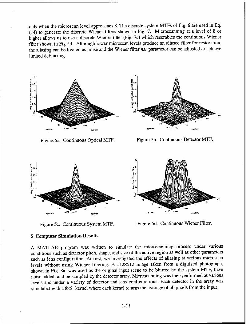
only when the microscan level approaches 8. The discrete system MTFs of Fig. 6 are used in Eq. (14) to generate the discrete Wiener filters shown in Fig. 7. Microscanning at a level of 8 or higher allows us to use a discrete Wiener filter (Fig. 7c) which resembles the continuous Wiener filter shown in Fig 5d. Although lower microscan levels produce an aliased filter for restoration, the aliasing can be treated as noise and the Wiener filter nsr parameter can be adjusted to achieve limited deblurring.

cyc/mm cyc/mm cyc/mm

Figure 5a. Continuous Optical MTF. Figure 5b. Continuous Detector MTF.

cyc/mm cyc/mm cyc/mm cyc/mm

Figure 5c. Continuous System MTF. Figure 5d. Continuous Wiener Filter.

5 Computer Simulation Results

A MATLAB program was written to simulate the microscanning process under various conditions such as detector pitch, shape, and size of the active region as well as other parameters such as lens configuration. At first, we investigated the effects of aliasing at various microscan levels without using Wiener filtering. A 512x512 image taken from a digitized photograph, shown in Fig. 8a, was used as the original input scene to be blurred by the system MTF, have noise added, and be sampled by the detector array. Microscanning was then performed at various levels and under a variety of detector and lens configurations. Each detector in the array was simulated with a 8x8 kernel where each kernel returns the average of all pixels from the input

1-11

Fig 6a. Discrete System MTF. L=l. Figure 7a. Discrete Wiener Filter Model. L=l.

Fig 6b. Discrete System MTF. L=4. Figure 7b. Discrete WienerFilter Model. L=4.

Fig 6c. Discrete System MTF. L=8. Figure 7c. Discrete Wiener Filter Model. L=8.

1-12

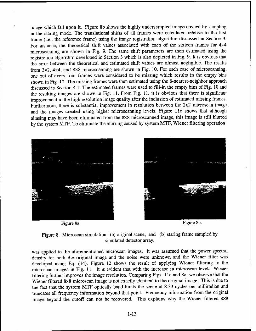
image which fall upon it. Figure 8b shows the highly undersampled image created by sampling in the staring mode. The translational shifts of all frames were calculated relative to the first frame (i.e., the reference frame) using the image registration algorithm discussed in Section 3. For instance, the theoretical shift values associated with each of the sixteen frames for 4x4 microscanning are shown in Fig. 9. The same shift parameters are then estimated using the registration algorithm developed in Section 3 which is also depicted in Fig. 9. It is obvious that the error between the theoretical and estimated shift values are almost negligible. The results from 2x2, 4x4, and 8x8 microscanning are shown in Fig. 10. For each case of microscanning, one out of every four frames were considered to be missing which results in the empty bins shown in Fig. 10. The missing frames were then estimated using the 8-nearest-neighbor approach discussed in Section 4.1. The estimated frames were used to fill-in the empty bins of Fig. 10 and the resulting images are shown in Fig. 11. From Fig. 11, it is obvious that there is significant improvement in the high resolution image quality after the inclusion of estimated missing frames. Furthermore, there is substantial improvement in resolution between the 2x2 microscan image and the images created using higher microscanning levels. Figure lie shows that although aliasing may have been eliminated from the 8x8 microscanned image, this image is still blurred by the system MTF. To eliminate the blurring caused by system MTF, Wiener filtering operation

Figure 8a. Figure 8b.

Figure 8. Microscan simulation: (a) original scene, and (b) staring frame sampled by simulated detector array.

was applied to the aforementioned microscan images. It was assumed that the power spectral density for both the original image and the noise were unknown and the Wiener filter was developed using Eq. (14). Figure 12 shows the result of applying Wiener filtering to the microscan images in Fig. 11. It is evident that with the increase in microscan levels, Wiener filtering further improves the image resolution. Comparing Figs. 1 lc and 8a, we observe that the Wiener filtered 8x8 microscan image is not exactly identical to the original image. This is due to the fact that the system MTF optically band-limits the scene at 8.33 cycles per milliradian and truncates all frequency information beyond that point. Frequency information from the original image beyond the cutoff can not be recovered. This explains why the Wiener filtered 8x8

1-13

microscan image is not exactly the same as the original input image. Therefore, the application of higher levels of microscanning may not yield better results.

x - Theoretical o - Shifts Associated with Simulated Frames

0.2 0.4 0.6 Horizontal shut h_k

Fig. 9. Theoretical and estimated registration parameters for 16 simulated frames.

6 Experimental Results

For experimental verification of the proposed algorithm, we applied the multiframe reconstruction and Wiener filtering technique to data collected on a real-time FLIR imaging system. The FLIR camera uses a 128x128 Amber AE-4128 infrared focal plane array with a 100 millimeter focal length f/3 lens. The focal plane array uses Indium-Antimonide (InSb) detectors with a response in the 3 to 5 micron wavelength band. The 100 millimeter lens was diffraction limited producing an optical cutoff of 8.33 cycles per milliradian. The system uses square detectors of size 50 microns with an 80% fill factor, making the active detector size of 40 microns with the remaining 10 microns being inactive. The information about the detector and lens configuration was used in our estimation of the system MTF, which was used for designing the Wiener filter during the computer simulation. The FLIR image data collected at Wright Laboratory using the Amber imaging system is shown in Figure 13. Three primary targets at a range of approximately 0.9 kilometers are contained in the image: a military truck, a civilian vehicle, and an M-60 tank. Figure 13a is one of the 16 staring image frames collected for a 4x4 microscan high resolution image. The staring image was then pixel replicated to the same size as the microscan image for comparison. The 4x4 microscan image is shown in Fig. 13b where the balnk horizontal lines shows that four (frames 13, 14, 15 and 16) out of the total of sixteen frames recorded have shifts similar to other frames i.e., four frames are missing. The missing frames were estimated using the procedure discussed earlier in Sections 4.1 and 5. The empty bins of Fig. 13b were filled with these estimated frames and the resulting microscan image is shown in Fig. 13c. The 4x4 microscan image after the application of Wiener filtering is shown in Fig. 13d. Notice that the application of Wiener filtering further increased the resolution of the 4x4 microscan image. The reason for this improvement is that by using Wiener filtering one reduces the blurring of the MTF which is responsible for suppressing the increase in image resolution that should be obtained at higher microscan levels. There appears to be slight ringing in the 4x4 microscanned image after the application of Wiener filter (Fig. 13d). This ringing is most noticeable in the boundary and in regions of high contrast, and is most likely the result of

1-14

phase distortions caused by the zero crossing values present in the system MTF. Figures 13e is the same as Fig. 13a but bilinear interpolation was used for the image replication. Comparing Fig 13c with 13d and 13e, it is evident that the proposed technique yields significantly improved image resolution even without Wiener filtering.

7 Conclusion

We have developed an efficient technique for real time infrared image registration and high resolution reconstruction by using multiple frames which are randomly shifted with respect to one another (uncontrolled microscanning). Such translationally shifted image sequences may be obtained by utilizing the random motion and/or vibration of the platform, such as an aircraft, on which the imager is mounted. A registration algorithm for estimating the random translational shifts among the multiple frames has been designed which is found to be inherently suitable for real time implementation. This algorithm can be used for estimating both non-integer as well as shift values larger than the detector width. However, with uncontrolled microscanning, some of the frames acquired by the imager may have shifts similar to other frames (missing frames) which results in empty bins in the high resolution image reconstruction. This problem has been tackled by developing a ^-nearest neighbor approach for estimating the missing frames so that it can be implemented in real time. Finally, Wiener filtering has been successfully applied as an effective means of reducing blurring in microscan images caused by the system MTF. A computer program which closely simulated the operation of the microscan system has been developed. The knowledge obtained from the microscan simulation was applied to real FUR data collected on the microscan imaging system. The results of the application of the Wiener filter to the microscan images confirmed the results obtained from the simulation data. It was found that Wiener filtering effectively reduces the effects of blurring and increases image resolution. This especially true with the real FUR data (compare Figs. 13c and 13d).

Future Research

Future research should address the following important issues: 1. In a practical scenario, the frames recorded by the FLIR array may be rotated as well as

translated with respect to each other. Therefore, it is essential to incorporate both the rotational and translational registration parameters in the high resolution image reconstruction.

2. Investigate the effects of detector nonuniformity (gain and bias drift) which creates fixed pattern noise on an image and developing a suitable algorithm to fix this problem.

3. Investigate the effects of both additive and multiplicative noise sources and develop a suitable algorithm to mitigate their effects.

4. Improving the interpolation techniques for calculating the missing frames for real time applications.

5. Investigating the effects of temporal blurring caused by factors such as atmospheric turbulence and alleviate such problems.

1-15

Acknowledgement

The authors would like to thank the following individuals for their assistance and support: John Bognar, Russell Hardie, Ernie Armstrong, Ken Barnard, Steve Cain, Brian Yasuda, Ed Watson, Donald Tomlinson, Paul McManamon and Dennis Cupp.

References

[I] A. Schaum and M. McHugh, "Analytic Methods of Image Registration: displacement Estimation and Resampling," Naval Research Report 9298, Feb. 28, (1992).

[2] E. A. Watson, R. A. Muse and F.P. Blommel, "Aliasing and blurring in microscanned imagery," Proc. of the SPIE, Vol. 1689, 242-250 (1992).

[3] R. C. Hardie and S. Cain, "MAP Estimation of a High Resolution Image From a Sequence of Undersampled Translationally Shifted Images," Under review, IEEE Transactions on Image Processing, February (1996).

[4] S. Cain and R. C. Hardie, "Restoration of Aliased Video Sequences via a Maximum- likelyhood Approach," To appear, Proceedings of the IRIS Symposium on Passive Sensors, Monterey, CA, March (1996).

[5] W. K. Pratt, Digital Image Processing, John Wiley and Sons, Inc., New York (1992).

[6] J. C. Gillette, T. M. Stadmiller, and R. C. Hardie, "Reduction of Aliasing in Staring Infrared Imagers Utilizing Subpixel Techniques," Optical Engineering, Vol. 34, pp. 3130-3137 (1995).

[7] M. Irani and S. Peleg, "Improving Resolution by Image Registration," CVGIP: Graphical Models and Image Processing, Vol. 53, pp. 231-239 (1991).

[8] E. Kaltenbacher and R. C. Hardie, "Infrared Image Registration and High Resolution Reconstruction," Proceedings of the National Aeronautics and Electronics Conference, pp. 702-709 (1996).

[9] R. C. Gonzalez and R.E . Woods, Digital Image Processing, Addison-Wesley, New York (1992).

[10] J. W. Goodman, Introduction to Fourier Optics, McGraw-Hill, Inc., New York, (1996).

[II] A. V. Oppenheim and R. W. Schäfer, Discrete Time Signal Processing, Prentice Hall, Inc., NJ, (1989).

[12] E. Armstrong, J. Bognar, B. Yasuda and R. C. Hardie, "The Appication of Wiener Filters to Microscan Imaging," To appear, Proceedings of the IRIS Symposium on Passive Sensors, Monterey, CA, March (1996).

1-16

Figure 10a. Figure 11a.

Figure 10b. Figure lib.

Figure 10c.

Figure 10. (a) through (c) are level 2,4 and 8 simulated microscan images with missing frames.

Figure 1 lc.

Figure 11. Restored images of Fig. 10 after estimating the missing frames.

1-17

Figure 12a. Figure 13a.

Figure 12b. Figure 13b.

Figure 12c.

Figure 12. Wiener Filtering. Figs. 1 la, b, and c are the Wiener filtered versions of Figs. 10a, b and c.

Figure 13c.

Figure 13. Real FLIR Images, (a) staring frame, (b) 4x4 microscan image, (c) restored image.

1-18

Figure 13d. Figure 13e.

Figure 13. Real FLIR Images, (d) restored image after Wiener filtering, (e) staring frame after bilinear interpolation.

1-19

ADDENDUM

High resolution infrared images may also be reconstructed from multiple translationally shifted aliased frames using iterative techniques such as Bayesian approach via maximum a posteriori (MAP) algorithm3 or maximum-likelihood approach via expectation maximization (EM) algorithm4. The MAP algorithm utilizes a prior statistical model for estimating the translational shifts. With this model, a maximum a posteriori estimator is used to estimate the high resolution image and the intraframe translational shifts. The shifts are iteratively updated along with the high resolution image using a suitable optimization technique such as gradient descent optimization. In the maximum-likelihood approach, the data are considered Poisson random variables and an EM algorithm is constructed that iteratively estimates an unaliased image compensated for the known imager system blur while simultaneously estimating the translational shifts. Both of these algorithms have been found to yield high resolution images from a sequence of randomly shifted frames. However, each of these algorithms require significant computation time and can not be implemented for real time applications using the currently available high performance microprocessors. The EM algorithm has been found to be faster than the MAP algorithm.

In this work, we have used the registration algorithm discussed earlier in Section 3 to estimate the translational shift parameters in just one step. Using this shift information, we have applied a simplified version of the EM algorithm to estimate the high resolution image from the given sequence of frames. The original EM approach recalculates the shits parameters with each iteration of the algorithm. The new image shift estimates are calulated by evaluating a cost function that compares the shifted and interlaced data frames to the corresponding values in the algorithm's latest high resolution image estimate. The cost function is the sum over all the pixels in the high resolution gird of the absolute value of the interlaced data frames divided by the high resolution image estimate. The shift parameters provided by the new registration algorithm are accurate enough to eliminate the need for iterative calculation of the translational shifts.

The proposed modified EM algorithm has been found to drastically reduce the computation burden compared to the original EM algorithm thereby making it more attractive for practical implementation. To verify the performance of the modified EM algorithm, let us consider the 16 staring FLIR real image data frames used in Section 6. One of these 16 staring FLIR image frames is shown in Fig. 13a. Using these 16 frames, the output obtained by the original EM algorithm4 and that obtained by the modified EM algorithm after ten iterations are shown in Figures 14a and 14b respectively. Comparing Figs. 14a with 14b, we observe that the modified EM algorithm yields high quality image and can be considered as a viable alternative to the original EM algorithm. For page number limitation, the author could not discuss this approach in detail in this report.

1-20

A FAST FOURIER TRANSFORM ANALYSIS OF PILOT INDUCED OSCILLATIONS

Dominick Andrisani, II Associate Professor

Sten E. Berge Graduate Student

School of Aeronautics and Astronautics Purdue University

West Lafayette, IN 47907-1282

Final Report for: Summer Faculty Research Program and Graduate Student Research Program

Wright Laboratory Wright-Patterson AFB, OH 45433


Boiling Air Force Base, DC

and

Wright Laboratory

August, 1996

2-1


Dominick Andrisani, II Associate Professor

Sten E. Berge Graduate Student

School of Aeronautics and Astronautics Purdue University

Abstract

During the summer of 1996 a program was initiated by the authors to study the

characteristics of pilot induced oscillations (PIOs). The long term goals are

• to develop a methodology to take time history data from flight or ground based

simulation and determine if a vehicle is PIO prone,

• to determine if a PIO actually occurred in a time history record,

• to develop a non-real-time analysis tool to determine from flight simulator time

history data if PIOs occurred so that simulation engineers can help insure

consistency between pilot comments, Cooper-Harper ratings, PIO ratings and time

history data, and

• to develop a real-time capability of detecting a PIO fast enough to take action to

prevent the full development of the PIO.

Results obtained over the period 7/1/96-8/23/96 deal primarily with the first goal

and are described in this report. A computer analysis tool is developed in which fast fourier

transforms are used to determine

• resonant frequency and output phase angles at the resonant frequency,

• predictions of PIO susceptibility using the Smith-Geddes PIO criteria.

The following preliminary results are highly encouraging.

• 13 of 14 configurations which experienced PIOs were correctly identified.

• In 12 additional configurations 6 were correctly identified as being not PIO prone.

Results for the remaining 6 configurations were complicated by multiple resonances

that confuse the resonance detector. However, depending on the choice of resonant

frequency the correct classification is made for each of the 6 configurations.

• The occurrence of multiple resonances is closely associated with configurations that

are not PIO prone.

• continued development of the resonance detector is planned.

2-2


Dominick Andrisani, II and Sten E. Berge

Background Pilot induced oscillations (PIOs) have received much recent attention [2-6]. Several

approaches to development of a unified PIO theory are currently being pursued. A catalog of

PIO events has been compiled and several existing criteria have been shown to successfully

predict PIO susceptibility. Accurate analysis of the ever-growing PIO database will gather

insight into the characteristics of PIOs. With this information, a PIO detector can be

designed for time history data as generated in either flight or simulation.

Discretization of Time History Data

Most PIO time history data in the catalog of PIO events is in paper copy form; the

original flight data having been lost or unavailable for various reasons. As a first step in

this analysis, various time history records from the PIO database were digitized. Eleven

classic PIOs and eighteen Bjorkman (NT-33) time histories [7] were digitized. The eleven

classic PIOs were taken from the PIO catalog compiled by HAI in cooperation with STI[2].

There is one roll ratchet, several rate limited actuator cases, mode switches, and both

lateral and longitudinal examples. The Bjorkman time histories are all longitudinal, but

provide a consistent database encompassing nearly the entire range of the PIO tendency

classification scale. The digitization was hampered by the quality of the reproductions and

the scales of the plots. Sections of data were often missing because of repeated previous

reproduction. Digitization noise was introduced into the data axis scaling was not well

chosen. For example, the B-2 charts cover too much time, and the non-PIO Bjorkman

configurations are plotted with the same scale as the large amplitude PIO histories.

Conversely, there were several data sets with time scaling that covered too small a time

period and which cut off the peaks of the data. The M2F2 charts are examples of this other

extreme.

The following multi-step digitization process was employed.

• PIO time histories were scanned and cleaned up using OFOTO commercial

software.

• PIO time histories were digitized the data using dataThief shareware.

• The resulting ASCII data file was converted to MATLAB script format.

2-3

• A MATLAB script was written to produce a second MATLAB script file with a

specified uniform time increment

• A MATLAB script was written to plot the time history data in a similar format to

the original.

In all 27 longitudinal records (flight records from the T-38, Shuttle, B-2, F-8, YF-22,

and X-15, 18 Bjorkman NT-33 flight records, and 3 HAVE PIO ground based simulation

records) and 5 lateral records (flight records from the F/A-18(2), F-14, YF-16, and M2-F2)

were digitized. These records are available at WL/FIGC-2 (Mr. David Leggett is the point of

contact, 513-255-8498).

Technical Approach A spectral analysis is performed on selected time histories to determine the

quantities needed for PIO characterization. The resonance of each measurement is

determined from power spectral density for that variable. The actual resonant frequency

will differ from the discrete frequencies used in the power spectral density plot, unless the

resonance happens to correspond to one of the harmonics of the spectral analysis. Therefore,

the resonant frequency is approximated by finding the centroid of the peak and its two

nearest neighbors. The cross spectrum between input and output is used to calculate a

frequency response function relating input and output. The phase angle at the resonant

frequency is taken from the phase angle of the frequency response function. The validity of

the results is related to the coherence of the cross spectral data points used.

The Smith-Geddes criteria are then evaluated. The pilot-vehicle resonant frequency

is chosen to be the resonant frequency of the variable with the most reliable time history.

This is most often pitch rate. The Smith-Geddes criteria require the phase angles of both

6(ja>)/F8(j<a) and Nz(j(ü)/FB(jfl>). The phase of 6(jä>)/Fg(joi) can also be calculated by

subtracting 90 degrees from the phase of q(jco)/F8(j(D). The Smith-Geddes analysis is done

with both the 6 and q phase angles. Susceptibility to PIO as defined in MIL-STD-1797A

[8], approximate Cooper-Harper rating, and approximate PIO rating based on Ralph Smith's

data method [10]are outputs of this analysis.

This procedure is not be completely automatic at this time for two reasons. First,

the FFT window size must be chosen subject to several constraints: the primary (lowest)

harmonic (set by the length of time (Twindow) used in the FFT, A(o=2Ä/Twindow) should be

approximately 1 rad/sec, and the highest harmonic (set by the time increment (AT),

©max=^AT) must be at least 20 rad/sec to include the resonant frequencies of all possible

types of PIOs including pitch bobbles and roll ratchets, the window not contain discrete

events such as control system mode switches, and at least two similar windows are required

2-A

to compute coherence. Second, the best pilot-vehicle resonant frequency must be manually

chosen when multiple resonances are present. Unless the same dominant resonant

frequency appears in all measurements, the correct choice is unclear. Further research on

this problem is continuing.

The spectral analysis is performed by MATLAB's spectrum function in the Signal

Processing Toolbox. The procedure used is Welch's averaged periodogram method [1,9].

Each frame consists of three subframes (two consecutive and one overlapping one half of the

other two). Each subframe is preprocessed by removing any bias and is windowed with a

Hanning window. Use of more than one subframe helps insure valid coherence. The

software steps through the time history frame by frame.

PIO susceptibility is determined by the Smith-Geddes criteria using the following steps.

• Pilot-in-the-Loop Properties

Resonant frequency, wr,

Amplitudes of inputs and outputs at wr from FFT data

©(M)> ?(M)> "«(M)

Pilot-Vehicle System Properties: Phase lags computed using Cross Spectral densities

Z e(ja>) F.tjco)

Z q(ja>) F.U'o»

Z nt(ja>) F.Ua»

• Smith-Geddes PIO Metrics

Use wr as the criterion frequency,

Determine susceptibility to

attitude type PIO (Type III) based on

z e(j(o) F.{j<0)

<-180 z q(j«>) F.Uco)

-90 < -180,

acceleration type PIO (Type I) based on

nU<o) <D(<a) = Z

Z Q(J(Q) F.(j<o)

F,U<o)

<-160

14. 3CO <-180 deg. when

2-5

A few comments are in order. We evaluate phase angles at the resonant frequency of

the pilot-in-the-loop system, wr. The Smith-Geddes criterion evaluates the phase angles at

the criterion frequency, wc = 0.24S + 6 where S is the average slope of the I q(ja>)/Fs(jca) I

over the interval from 1-6 radians per second, wc is an approximation to the crossover

frequency of the pilot-vehicle system during pitch attitude tracking. If there is a dominant

resonance in a time history record our approach is reasonable since the pilot-vehicle system

will resonate near the crossover frequency of the pilot-vehicle system.

Our approach is more than an open loop method because our resonant frequency is a

property of the pilot-vehicle system as expressed in the time histories from the piloted

system.

Problems with the Resonant Frequency Dutectar

Several problems were encountered with our resonant frequency detector.

• Power spectra of important traces sometimes have multiple peaks. Figure 1

shows an example of a time spectrum with two resonant peaks. Figure 2 shows the more

common case where there is a single dominant resonant peak.

• Power spectra of different traces sometimes have different peaks as shown in the

sketch below.

Power

Power

Frequency

• Low frequency power sometimes confuses our resonant frequency detector. Figure 1

also illustrates this problem.

There are several possible solutions to those problems. Multiple peaks on one power

spectrum and peaks that don't line up seem to correlate with the absence of PIO. Low

frequency power might be removed by a different choice of windowing in computing the FFT

2-6

or by filtering the time history before the FFT is taken. We are currently using a Hanning

window. The end of the summer prevented our resolution of the problems. Development of the

resonant frequency detector will continue until the end of 1996 by Professor Andrisani.

Bßfllltft

The results from our analysis of longitudinal PIO data are summarized in Tables 1

and 2. PIO amplitudes versus resonant frequency is shown in Figure 3. The longitudinal

PIOs in this study occur at a wide range of amplitudes. This suggests amplitude of the

resonance is not a good metric to determine if a PIO is occurring.

Angle * (of the Smith-Geddes criterion [10]) versus actual average PIO rating for the

Bjorkman data is shown in Figure 4. The line in the figure comes from [10] and seems to

underestimate the average PIO ratings. Average Cooper-Harper ratings versus angle of

e(jü))/F8(jco) is shown in Figure 5. Figure 6 shows that the occurrence of a PIO seems to correlate well with a single

dominant resonant frequency in the time history. This characteristic seems more helpful in

determining that a PIO has occurred than output amplitude at the resonant frequency.

More work is required here to determine how to effectively use this fact

Table 1 indicates that acceleration type PIO were important in detecting PIO

susceptibility in only 1 of 24 cases (B2). The need for acceleration type PIO is currently

under review by the authors. These results indicate that the Smith-Geddes boundaries are

reasonable. When phase angles vary significantly during a time history nonlinear behavior is

suspected. One cause of this is rate limiting, where phase lag is a function of amplitude and

frequency. The Shuttle record, Figure 7, show« strong time varying phase angle of

q(j<D)/Fs(j©). The B2 record, Figure 8, shows almost no time varying phase angle of

q(j<ö)/F8(jö>). The ability of this method to track time varying phase angles is significant

because this can trigger a PIO.

TW,rH« H Time Domain PIO Detector.

The following comments summarize the status of our efforts at developing a FFT

Based PIO detector. • The existing algorithm is not set up to run in real time. A Wright Laboratory in-

house effort by Mr. Phil McKeehan is anticipated in this area.

2-7

• Some operator intervention is helpful in selecting the time periods to analyze so

that PIO events are not split into different time frames.

• Improvement is necessary on the resonant frequency detector.

• We still need to determine in what way amplitude at resonant frequency is helpful

for PIO detection.

• We need to decide what the occurrence of multiple resonances indicates about PIO.

Conclusions Based on recently digitized time histories of 27 longitudinal PIOs the following

conclusions are drawn.

• Our FFT Based PIO Analysis Software using the Smith-Geddes criteria does an excellent

job of determining PIO susceptibility.

• Preliminary results indicate that the Smith-Geddes boundaries are reasonable.

• Acceleration type PIO were important in detecting PIO proneness in only 1 of 24 cases

(B2). The need for this characterization is under continuing review.

• Continued development of the resonant frequency detector is required for cases where

multiple resonances occur.

• The ability of this method to track time varying phase angles is significant because this

can serve as a trigger for PIOs.

Further Work During Professor Andrisani's sabbatical at Wright Laboratories (8/19/96-12/20/96)

the additional work on the following items is planned.

• resonant frequency detector,

• adequacy of the Smith-Geddes boundaries,

• need for acceleration type PIOs,

• importance of multiple resonances in PIO detection,

• automating the analysis process to achieve the third goal mentioned in the

abstract.

An in-house Wright laboratory effort is anticipated to develop and implement a real

time PIO detector based upon this work.

Acknowledgments This work was conducted under the Summer Research Program supported by the Air

Force Office of Scientific Research at Wright Laboratory, Wright-Patterson AFB. The focal

points were Wayne Thor (513-255-8497), David Legget and Tom Cord.

2-8

References 1. Bendat, Julius S. and Allan G. Pip.rsol. Engineering Applications of Correlations and

,qPAH-.r»l Analysis. John Wiley & Sons, New York, 1980.

2. Mitchell, David G. and Hoh, Roger H. , Development of a Unified Method To Predict

Tendencies for Pilot-Induced Oscülations, WL-TR-95-3049, June 1995.

3. Klyde, David H., Duane T. McRuer, and Thomas T. Myers, Unified Pilot-Induced

Oscillation Theory, Volume 1: PIO Analysis with Linear and Non linear Effective Vehicle

Characteristics, Including Rate Limiting, WL-TR-96-3028, December 1995.

4. Preston, Jeff D., Hodgkinson, John, and Buckley, Jim, Unified Pilot-Induced

Oscillation Theory, Volume II: Pilot Induced Oscillation Criteria Applied to Several McDonnell

Douglas Aircraft, WL-TR-96-3029, December 1995.

5. Anderson Unified Pilot-Induced Oscillation Theory, Volume 1: PIO Analysis with

Linear and Non linear Effective Vehicle Characteristics, Including Rate Limiting, WL-TR-96-

3028, December 1995.

6. Bailey, Randall E. and Bidlack, Timothy, J., Unified Pilot-Induced Oscillation

Theory, Volume 2V: Time Domain Neal-Smüh Criteria, WL-TR-96-3031, December 1995.

7. Bjorkman, Eileen A. Flight Test Evaluation of Techniques to Predict Longitudinal

Pilot Induced Oscillations, M.S. Thesis, Air Force Institute of Technology, AFIT/GAE/AA/86J-

1, December 1986.

8. Military Standard, Flying Qualities of Piloted Aircraft, MIL-STD-1797A, revised 28

June 1995.

9. Welch, Peter D., The Use of Fast Fourier Transform for Estimation of Power

Spectra: A Method Based on Time Averaging Over Short, Modified Periodograms, IEEE

Trans. Audio and Electroacoust., vol. AU-15, pp. 70-73, June 1967.

10 Smith, Ralph H., "The Smith-Geddes Handling Qualities Criterion," 1994 SAE

Aerospace Atlantic Conference, Dayton, OH, April 20,1994.

2-9

Table 1. Summary of Numerical Results for Longitudinal PIOs.

PHASE LAG ANALYSIS Long. PtO from Right

Aircraft wr ThetaWrdeg qWrdeg nzWrdeg phi

PIO in time history T-38 7.49 -268 -234 -248 -355 Shuttte(t«24-30) 2.40 NaN -153 NaN NaN Shuttte(t«26-32) 3.40 NaN -171 NaN NaN B2 (t=25-31.7) 3.63 -165 -8 -138 -190 F8(t=8.1-20.6) 2.79 -220 -144 -185 -225 YF-22 3.25 -213 -121 -197 -243 Bjorkman 2-5 2.57 -208 -125 -196 -232 Bjorkman 2-8 4.33 -219 -126 -174 -236 Bjorkman 3-12 1.91 -162 -72 -126 -154 Bjorkman 3-13 3.21 -184 -130 -178 -224 Bjorkman 5-9 3.51 -227 -122 -185 -235 Bjorkman 5-10 2.81 -195 -119 -176 -216 HAV£,4/13,#21(Bj3-13) 1.32 -277 -196 -261 -279 HAVE, 4/13,#22(Bj3-13) 1.13 NaN -195 -271 -287 HAVE,4/13,#23(Bj3-13) 1.76 -320 -236 -322 -348

no PIO in time history Bjorkman 2-B 4.95 -123 -74 -137 -207 Bjorkman 2- 1(wr-1.1) 1.12 -70 37 -93 -109

(wr-5.4) 5.43 -266 -97 -178 -256 Bjorkman 3-D 6.88 -180 -89 -32 -130 Bjorkman 3-1 1.78 -67 14 -67 -93 Bjorkman 3-3 3.51 -119 -47 -114 -165 Bjorkman 3-6 (wr-8.9) 8.87 -203 -108 -36 -163

(wr-3.0) 3.00 -105 -13 -50 -93 Bjorkman 4-1 (wr-6) 5.97 -174 -94 -141 -227

(wr-10) 10.00 -277 -122 -340 -483 (wr-2.5) 2.52 -120 -8 -92 -128

Bjorkman 4-2 4.83 -155 -65 -129 -198 Bjorkman 5-1 2.37 -100 -35 -100 -133

maybe PIO in time history Bjorkman 2-7(t« 14-29) 4.29 -197 -119 -138 -200

(t-22-29, wr-4.3) 4.28 -194 -119 -144 -205 (t=22-29,wr«6.1) 6.12 -241 -149 -120 -208

Bjorkman 3-8 7.03 -246 -155 -117 -217 Bjorkman 5-11 (wr-2.5) 2.50 -202 -113 -142 -178

(Vtf-1.9) 1.87 -147 -56 -108 -135 (wr-3.2) 3.32 -229 -137 -145 -193

2-10

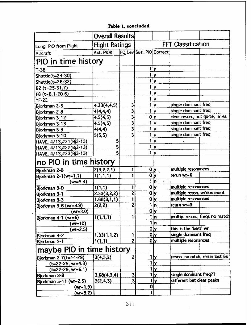
Table 1, concluded

Overall Results

Long. PIO from Flight Flight Ratings FFT Classification

Aircraft Act. PIOR FQLev Sus_PI0 Correct

PIO in time history T-38 y Shuttle(t«24-30) y Shuttle(t-26-32) y B2(t=25-31.7) y F8(t-8.1-20.6) y YF-22 y Biorkman 2-5 4.33(4,4,5) 3 y single dominant freq

Bjorkman 2-8 4(4,4,4) 3 y single dominant freq

Bjorkman 3-12 4.5(4,5) 3 0 n clear reson., not quite, miss

Bjorkman 3-13 4.5(4,5) 3 y single dominant freq

Bjorkman 5-9 4(4,4) 3 y single dominant freq

Bjorkman 5-10 5(5,5) 3 y single dominant freq

HAVE,4/13,#21(Bj3-13) 5 y HAVE,4/13,#22(Bj3-13) 5 y HAVE.4/13.#23(Bj3-13) 5 y

no PIO in time history Bjorkman 2-B 2(3,2,2,1) 1 0 y multiple resonances

Bjorkman 2- 1(wr« 1.1) 1(1,1,1) 1 0 y rerun wr«6

(wr-5.4) 1 n

Biorkman 3-D 10,1) 1 0 y multiple resonances

Biorkman 3-1 2.33(3,2,2) 2 0 y multiple reson. w/dominant

Bjorkman 3-3 1.68(3,1,1) 1 0 y multiple resonances

Bjorkman 3-6 (wr-8.9) 2(2,2) 2 1 n reumwr-3

(wr-3.0) 0 y Bjorkman 4-1 (wr-6) 10.1,1) 1 1^ n murtip. reson., freqs no mate*

(wr-10) 1 n

(wr-2.5) 0 y this is the'best* wr

Biorkman 4-2 1.33(1,1,2) 1 0 y single dominant freq

Biorkman 5-1 10.1) 2 0 y multiple resonances

maybe PIO in time history Bjorkman 2-7(t-14-29) 3(4,3,2) 2 1 y reson. no mtch, rerun last 6s

(t=22-29, wr-4.3) 1 y (t=-22-29,wr«6.1) 1 y

Bjorkman 3-8 3.68(4,3,4) 3 1 y single dominant freq??

Bjorkman 5-11 (wr=2.5) 3(2,4,3) 3 1 y different but c ear peaks

(wr-1.91 0 (wr-3.2) 1

2-11

Table 3. Summary of PIO Classification Results

Configurations Results 14 PIO-prone Configs correct classification: 13

Bjorkman8 configs with wrong classification: 1 PIOR consistently >4 (Bjorkman 3-12)

T-38, Shuttle, B-2, F-8, YF-22 (There was a clear single dominant S HAVE PIOs (Bjorkman 3-12) frequency.)

9 not PIO-prone Configs correct classification: 6 Bjorkman Configs with correct by choice of wn 3

PIOR consi8tently<4 wrong classification: 0

S maybe PIO Configs correct by choice of wn 3 at least 1 PIOR »4 wrong classification: 0 ( Bjorkman 2-7, Config(PIOR) Bjorkman 3-8, Bj2-7(4&2) PIO-prone at 3/3 wrs Bjorkman 5-11) BJ3-8 (4A4) PIO-prone at 1/1 wrs

Bi5-ll(2,4.3) PIO-prone at 2/3 wrs

2-12

Resonance from Pilot input. Bjorkman config. 2-1. Time=( 0.01 -14.49) sec

N

%

%3h

<D

O B2

Resonant Frequency= 1.06 r/s

x

*

x *XK ?K * ^ Ä Ä ill **tt:»ix*yxxxxx

10 15 20 frequency (rad/sec)

25 30

Figure 1. Power spectrum showing multiple resonances and low frequency power

2-13

1200

1000-

Resonance from Pilot Input, F8, Tlme=( 8.08 - 20.57) sec T

N 800-

§ 600

400

200-

10 15 20 frequency (rad/sec)

25 30 35

Figure 2. Power spectrum showing a single dominant frequency

2-14

o o 00

o < 4- 9

o - °. (D

O O

n O E o 0L

o o

i

> o e • 3

o E m

o -- °.

o _- o

o o

o o d

o o to CM

o o

CM

o o

o o

o o

o o

(o«8/C«p)b to •pnuiduw

Figure 8. Properties of Longitudinal PIOs

2-15

at c CO CC O 5Z

i

-V ■

_ v—

o w m

© o CO

o u> CM

O O C4

O m

o o

o 10

to in in o w c\j

OufieU OW "»Ay

w «- in

Figure 4. Actual average PIO ratings versus phi for Bjorkman records

2-16

c (0 cc O K

s.

< 1

\

<

i ►

♦

o

< ► N

■

\

\

\ \

-

o CM

O

CM

o CM CM

O O CM

O CD

O to

**

2 ?

o o

o

o (0

o CM

IO CM]

ßunea HO "CAV

Figure 5. Actual average Cooper-Harper ratings versus phase of ©(jtOrVFsOör) for Bjorkman records

2-17

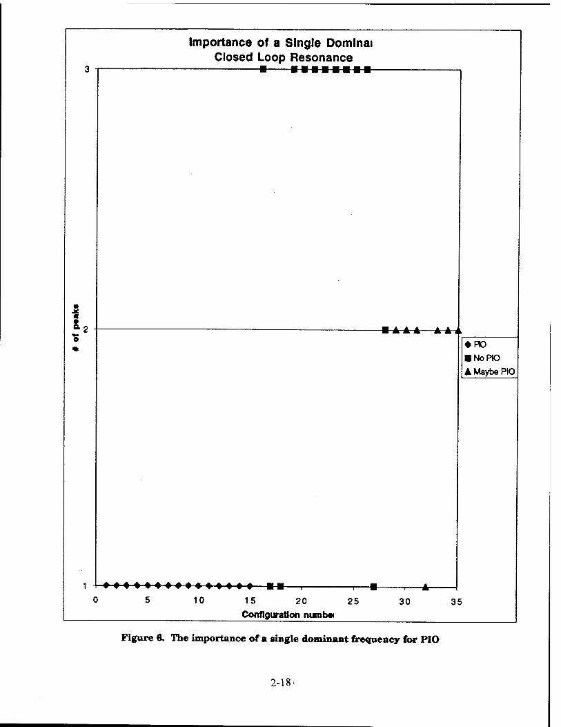
Importance of a Single Domlnai Closed Loop Resonance

e *

iVA—A-ä-ii ♦ PO

■ NoPK) A Maybe PIO

1 +■

10 15 20 25

Configuration numb« 30 35

Figure 6. The importance of a single dominant frequency for PIO

2-18-

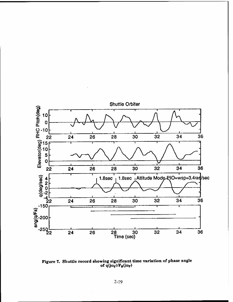
Shuttle Orbiter

IO=wsp=3.4ra« /sec

28 30 Time (sec)

Figure 7. Shuttle record showing significant time variation of phase angle of q(jöJr)/Fg(Jö>r)

2-19

B-2

25 30 Time (sec)

Figure 8. B2 record showing insignificant time variation of phase angle of qOörWgtfcor)

2-20

TEXTURE AND MICROSTRUCTURE OF HOT ROLLED Ti-6A1-4V

Pnina Ari-Gur Associate Professor

Department of Construction Engineering, Materials Engineering & Industrial Design

Western Michigan University Kalamazoo, MI 49008-5064

Final Report for: Summer Faculty Research Program

Wright Laboratory



and

Wright Laboratory

September 1996

3-1

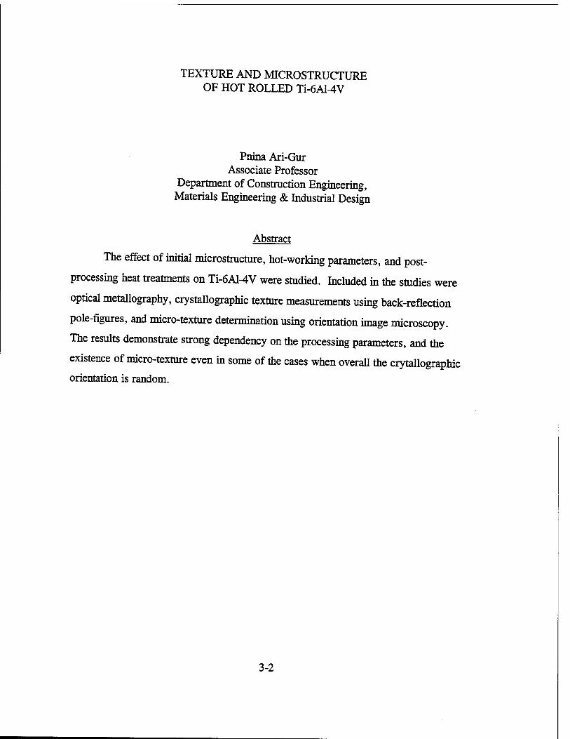
TEXTURE AND MICROSTRUCTURE OF HOT ROLLED Ti-6A1-4V

Pnina Ari-Gur Associate Professor

Department of Construction Engineering, Materials Engineering & Industrial Design

Abstract

The effect of initial microstructure, hot-working parameters, and post-

processing heat treatments on Ti-6A1-4V were studied. Included in the studies were

optical metallography, crystallographic texture measurements using back-reflection

pole-figures, and micro-texture determination using orientation image microscopy.

The results demonstrate strong dependency on the processing parameters, and the

existence of micro-texture even in some of the cases when overall the crytallographic

orientation is random.

3-2

TEXTURE AND MICROSTRUCTURE

OF HOT ROLLED Ü-6A1-4V

Pnina Ari-Gur

Introduction:

Ti-6A1-4V is a high-strength light-weight material that has been in extensive use

for aerospace applications. Its processing is difficult — it is not workable at low

temperatures, while at temperatures above 75% of the solidus temperature, its

developing microstructure is hard to control [1].

At room temperature and up to 1815°F, Ti-6A1-4V has a dual phase (a+ß)

structure. The a-phase (HCP), the dominant phase throughout this temperature range,

is highly anisotropic in nature. The second phase (ß) is BCC, and is the single phase

present above the transus temperature (1815°F). Numerous studies investigated the

relationship between processing and crystallographic texture development in dual-

phase titanium alloys and its effect on the mechanical properties. However, failure

analyses done on Ti-6A1-4V parts often reveal that even in the absence of overall

preferred orientation (texture) in the part, aligned a colonies provide nucleation site for

internal fatigue cracks. This phenomenon may result in a ten-fold decrease in fatigue

life [2,3]. The aligned a colonies can be traced back to the original ß (BCC) grain that

existed above the transus temperature. Breaking the original microstructure, as well as

3-3

elimination of the micro-texture (local aligned colonies), are what thermo-mechanical

processing [1] is aimed at.

The goal of this work was to study the effects of initial microstructure, assorted

hot-rolling parameters, and several post-processing heat treatments on the evolution of

microstructure, crystallographic texture, and micro-texture.

2. EXPERIMENTAL PROCEDTTRF.S

2.1 Processing:

The as-received plate of Ti-6A1-4V (1.17" thick) was divided to two groups,

that were heat treated differently to provide different initial microstructures. Each one

was heat treated in preparation for the hot rolling. These are summarized in Table 2.1.

Table 2.1 Pre-processing Heat Treatments

Group 1 (ß annealed)

Temperature 1725T 20 min

1950T 15 min

1725T 5 min

1500°F 15 min

Air cool Time |

Group 2 (ß quenched)

Temperature 1 1725°F 1950T Water Quench Time | 20 min 15 min

The 1725T and 1500°F treatments, following the 15 min at 1950°F for group 1,

were intended to simulate the slow cooling of large billets.

To study the development (or breakdown) of structure during the process,

specimens were hot rolled to two levels of strains:

• Light reduction (sT = 0.57, from 1.17" to 0.658")

• Heavy reduction (sT = 1.5, from 1.17" to 0.27" )

3-4

Three rolling temperatures were chosen in consideration of the ß transus

temperature (1815°F) and the minimum temperature where Ti-6A1-4V is still workable.

The rolling temperatures were:

• 1780T

• 1700T

• 1500T

To guarantee temperature uniformity, specimens were placed in the furnace for

40 minutes prior to rolling. The reduction per rolling pass was 10% (except for the

rolling at 1500°F that was performed at 5% reduction per pass). Between passes, the

specimens were re-heated for 3 minutes.

To study the effect of dynamic versus static recrystalliztion, some of the

specimens were heat treated following the hot-rolling. These heat treatments are

summarized in Table 2.2. Group number four (as-hot rolled) was tested

metallographically only. The heat treatment at 1300°F is for relieving stresses only and

does not change the structure or texture. It was needed for the micro-texture studies,

due to the sensitivity of the orientation imaging technique.

Table 2.2 Post-processing Heat Treatments

Group Number Temperature Time Cooling 1 Same as rolling 2 hours Air 2 1600°F 2 hours Air 3 1750°F 2 hours Air 4 As hot rolled N/A N/A 5 1300°F 1 hour Air

3-5

2.2 Testing

The microstructure, crystallographic texture, and micro-texture of the hot-rolled

and heat-treated samples were characterized by regular optical metallography, x-ray

diffraction, and orientation imaging microscopy. For the sake of comparison, the pre-

rolling, as heat treated plates were tested too.

2.2.1 Metallography

Metallographic samples were sectioned parallel to the N-R plane (perpendicular

to the transverse direction), polished and etched for 15 seconds in Kroll's solution (3.5

vol% HN03, 1.5 vol% HF, balance H20). Specimens of as-hot rolled, as well as heat

treated (Table 2.2) were photographed.

2.2.2 Texture

X-ray diffractometer (Cu Kcc radiation) equipped with pole-figure goniometer

was used for the crytallographic texture studies. Basal plane (0002) pole figures were

created for samples cut and polished in the R-T plane (parallel to the rolling plane about

2.5mm below the surface). Only back reflection data were collected (maximum tilt of

80°).

2.2.3 Micro-texture

Samples were cut, mechanically polished and electro-polished parallel to the N-

T plane (perpendicular to the rolling direction). The electro-polishing was necessary to

remove any surface damage left after the careful mechanical polishing. Two areas of

3-6

2mm x 2mm each were scanned (1mm x 4mm for the heavily rolled samples), one close

to the rolling surface, and the other — at mid-section).

Icosahedral maps were plotted for the basal (0002) plane. They were based on

40,000 points of measurement each. Each indexed point is within 0.9° of an

icosahedral face (or else the program determines that it is unable to index it and the

point appears white on the map).

In addition to the icosahedral maps, pole-figures (parallel to the N-T and to the

R-T plane) were drawn reflecting the average texture in each scanned area.

3. EXPERIMENTAL RESULTS AND DISCUSSION

3.1 Micro-structure

The microstructures of the pre-processing heat treated samples are shown in

Figure 1. As expected, the ß-annealed sample (Figure la) demonstrates a coarse,

basket-weave (Widmanstatten) type structure, while the ß- quenched sample has a lot

finer microstructure (Figure lb).

Even relatively large deformations (s=1.5) at 1500°F resulted in a non-uniform

microstructure (Figure 2). Post-rolling heat treatment at 1500°F does little, if at all to

change the previously deformed microstructure (Figure 3). At the higher temperatures

tested , recrystalliztion occurs, and heat treatment at 1750°F following the rolling,

results in equiaxed structure (Figure 4).

3-7

At the other end, rolling at 1780T, resulted in non-uniform deformation only at

small strains (s=0.57, Figure 5a). Subsequent deformation to s = 1.5 at this

temperature, resulted in a uniform microstructure (Figure 5b). Post-deformation heat

treatment at 1600°F merely coarsened the microstructure of the lightly rolled specimens

(Figure 6a), but resulted in basket-weave like structure for the heavily rolled specimen

(Figure 6b). It seems as if the subsequent deformation has triggered an earlier

transformation.

Figure la: Microstructure of the pre-processing ß-annealed sample.

3-8

Figure lb: Microstructure of the pre-processing ß-quenched Sample.

Figure 2 Microstructure of a sample that was ß-annealed and hot-rolled (e=1.5) at

1500°F.

3-9

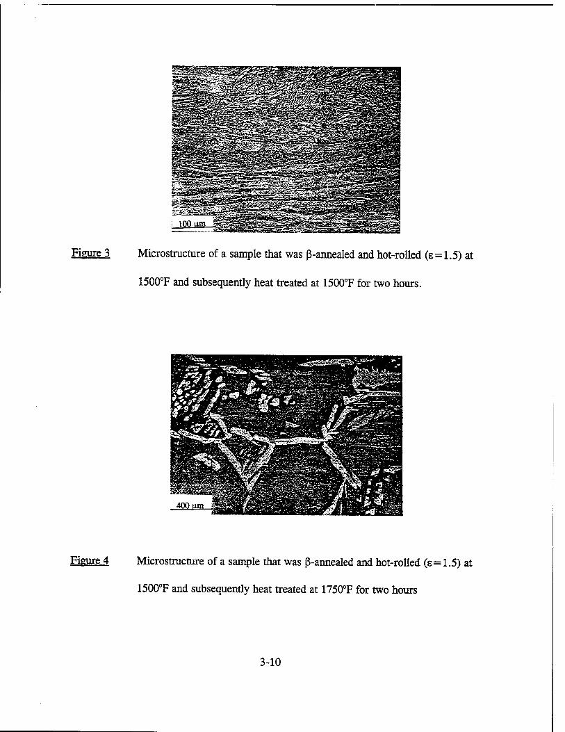
Figure 3 Microstmcture of a sample that was ß-annealed and hot-rolled (s=1.5) at

1500°F and subsequently heat treated at 1500°F for two hours.

Figure 4 Microstmcture of a sample that was ß-annealed and hot-rolled (s = 1.5) at

1500T and subsequently heat treated at 1750°F for two hours

3-10

Figure 5a Microstructure of a sample that was ß-annealed and lightly hot-

rolled (s=0.57) at 1780°F.

lö

rfr E*T **"?C:

^5Q9EC?*WB/

i«^S £JJB^^JgiP

.a -^ ?jJr7j|B^*' —'.•"; rarri^ £-± *"nrir ~A*5?*^

S5S5ä5y=3 •jjlsfiiäf;

"jLt^^LL ' Jj

fg§s|§ _100iim J

Figure 5b Microstructure of a sample that was ß-annealed and heavily hot-

rolled (s=1.5) at 1780°F.

3-11

Figure 6a Microstructure of a sample that was ß-annealed and lightly hot-

rolled (s=0.57) at 1780°F and subsequently heat-treated at

1600°F for two hours.

Figure 6b Microstructure of a sample that was ß-annealed and heavily hot-

rolled (s=1.5) at 1780°F and subsequently heat-treated at

1600°F for two hours.

3-12

3.2 Crvstallographic Texture

Pole-figures of the (0002) plane for the ß-annealed ß-quenched plates are

presented in Figure 7. Both demonstrate preferred orientation. Although the large

grain-size may make the texture appear stronger than it is, its consistency and four-fold

symmetry serve as a proof of its existence. The two texture components both of them

demonstrate, are in the transverse direction, and at about 45°. Rolling the plate at

1780°F (Figure 8) retained the TD texture, but eliminated the 45° and prompted an RD

texture to develop. Based on the literature [4], the appearance of the RD texture was

not expected for deformation below the transus. It is possible that the oxygen levels

(resulting from heat treatment in air) in our samples were different than the literature

and caused a shift in their location in the phase diagram.

Itou Iwlatiw • L* m- *» IwitiMM • *3 a*, flan «nu hnu IMM* • UtlTI * HtM • a-U «f liaytii > M.M «f. Imp MIT ■ 44.» Of.

NTMllaOKltr* 411 tUM>IM«Mii I*JM

pi.n

_. V A. >-~^Jl 1.1/ • «

l| LM1UM HUJt-IUti

Figure 7a: Pole-figures of the (0002) plane for the ß-annealed plate.

3-13

KÜM M« I**» total«*« « M l*. F»l to*HUai - «.• • MM.uMiRi Htm« aji*»- hoy—ii ■ a.a*«i. iiw litttutr ■ »U ■«*» tot»»» - m

-a. t

n TIM'/

II .»-UM C l LK- L*l l(LH<MN [(Mt* UM f ( MI-U.M Kiurtuu

Figure 7b: Pole-figures of the (0002) plane for the ß-quenched plate.

«Murwc fwwam Hat nttt fa-alao« • 2.1 «i. m taa-iattaa - M a*.

toiiM lit-awtr • »O ■■>»*• tot-awt- • 32

V. V t ii~-/—= - ' -r^ i

.I!.B-I..I \, -Cr-^1-—^-^^'-^^ -'

Figure 8: Pole-figures of the (0002) plane for the specimen rolled at 1780°F.

3-14

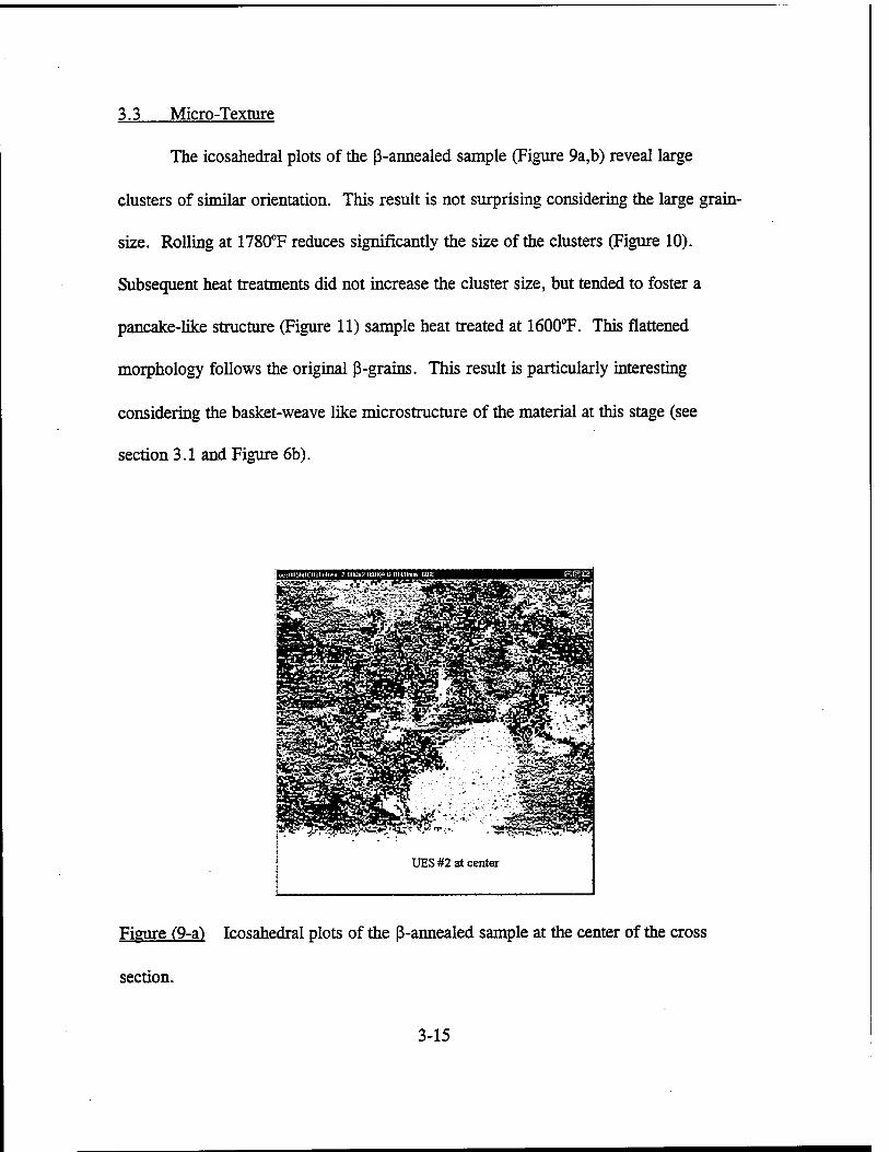
3.3 Micro-Texture

The icosahedral plots of the ß-annealed sample (Figure 9a,b) reveal large

clusters of similar orientation. This result is not surprising considering the large grain-

size. Rolling at 1780°F reduces significantly the size of the clusters (Figure 10).

Subsequent heat treatments did not increase the cluster size, but tended to foster a

pancake-like structure (Figure 11) sample heat treated at 1600°F. This flattened

morphology follows the original ß-grains. This result is particularly interesting

considering the basket-weave like microstructure of the material at this stage (see

section 3.1 and Figure 6b).

Figure (9-a) Icosahedral plots of the ß-annealed sample at the center of the cross

section.

3-15

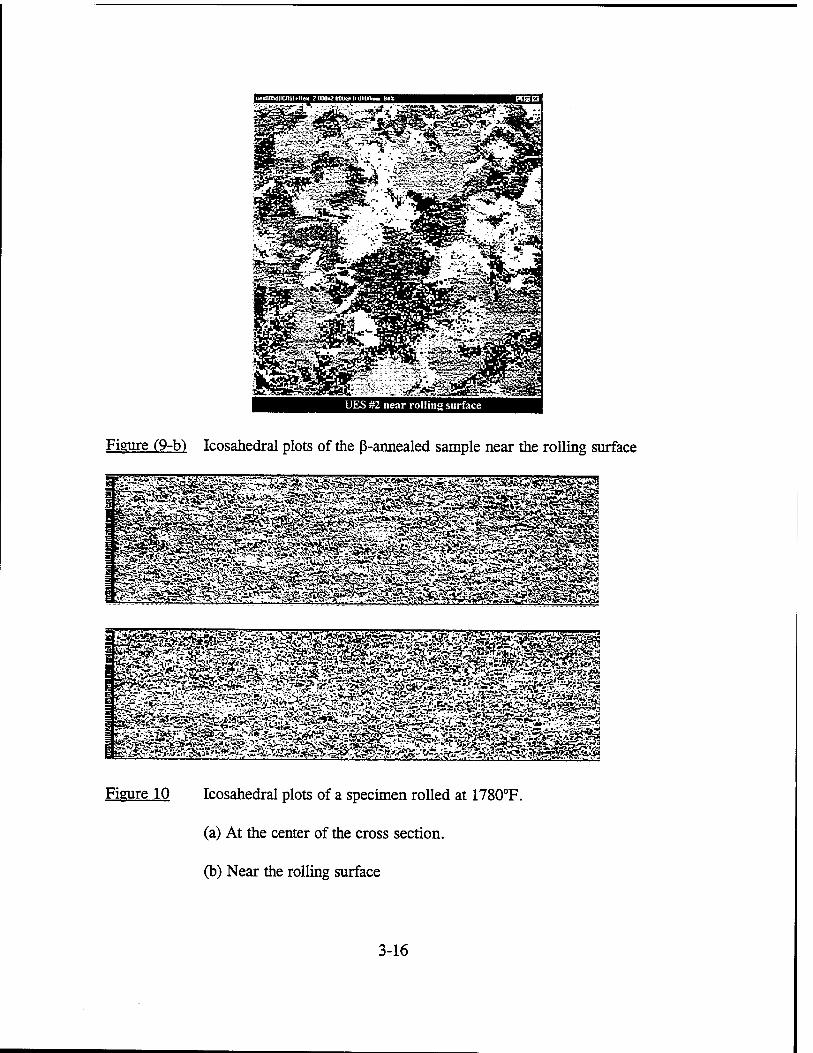
ueiOOMIIUHii-Hen 2 WS0*2 ÜO0(^ 0 ÜWOtnm »42

UES #2 near rolling surface

Figure (9-b) Icosahedral plots of the ß-annealed sample near the rolling surface

Figure 10 Icosahedral plots of a specimen rolled at 1780T.

(a) At the center of the cross section.

(b) Near the rolling surface

3-16

[email protected]ömm 70S

Sample 722 near surface

Figure 11 (a) Icosahedral plots of a specimen rolled at 1780°F then heat treated at

1600T. Scan taken from the area near the rolling surface.

Figure 11 (b) Icosahedral plots of a specimen rolled at 1780T then heat treated at

1600°F. Scan taken from the area near the center of the cross section

3-17

SUMMARY:

1. The samples that underwent heat treatment only, demonstrated large clusters with

similar orientation. The microstructure is a typical basket-weave.

2. Light rolling the heat-treated plates resulted in a highly non-uniform deformation

throughout the temperature range studied.

3. Heavy rolling close to the transus temperature resulted in a uniform deformation.

4. Heat treating the previously hot rolled samples may have fostered a pancake-like

arrangement of the crystallographic orientations, that may be correlated with the

original ß-grains.

RECOMMENDED FUTURE STUDIES:

1. Orientation imaging microscopy studies of the evolution of micro-texture in samples

that were ß-quenched and subsequently hot rolled and heat treated.

2. Complete studies of samples rolled at 1725T and 1750°F. From the results

reported here, it seems as if the 1780°F temperature resulted with substantial

transformation to ß, testing of samples rolled at lower temperatures, will enable us

to study the effect of a-phase deformation at elevated temperatures.

3-18

ACKNOWLEDGEMENTS:

Special thanks to Dr. Lee Semiatin for his contribution in numerous discussions

and for his continued encouragement. Thanks also to Keith Krueger of Lambda

Research for the x-ray diffraction, to John Sutliff and Scott Sitzman of General Electric

for the OJM, and to Robert Lewis for his help with the metallography.

REFERENCES:

1. Semiatin, S. L., et al, "Hot Working of Titanium Alloys - an Overview", in Weiss,

I., et al, eds., Advances in the Science and Technology of Titanium Processing,

TMS, 1996.

2. Woodfield, A. P., et al, "Effect Of Microstructure On The Dwell Fatigue Behavior

Of Ti-6242", in Eighth World Titanium Conference, Birmingham, England,

October, 1995.

3. Semiatin, S. L., and Eylon, D., Private communication, 1996.

4. Williams, J. C. and Starke, E. A., "The Role of Thermomechanical Processing in

Tailoring the Properties of Aluminum and Titanium Alloys", in Krauss, G., ed.,

Deformation, Processing, and Structure, (Materials Park, OH, 1984), 279-354.

3-19

STATISTICAL ANALYSIS OF FATIGUE CRACK GROWTH RATE DATA FOR 7075-T6 ALUMINUM DAMAGED BY PRIOR CORROSION

J.D. Baldwin Assistant Professor

School of Aerospace & Mechanical Engineering

University of Oklahoma 865 Asp Avenue, Room 212 Norman, Oklahoma 73019

Final Report For Summer Faculty Research Program

Wright Laboratory, Flight Dynamics Directorate Wright-Patterson Air Force Base

Sponsored By: Air Force Office of Scientific Research

Boiling Air Force Base, D.C.

August 15,1996

4-1

ANALYSIS OF FATIGUE CRACK GROWTH RATE DATA FOR ALUMINUM ALLOYS DAMAGED BY PRIOR CORROSION

J.D. Baldwin Assistant Professor

School of Aerospace & Mechanical Engineering University of Oklahoma

Abstract

The differences in fatigue crack propagation behavior in 7075-T6 aluminum alloy between

specimens damaged by corrosion and those in a baseline (noncorroded) condition are examined

using a statistical hypothesis test. Middle tension plate specimens were corroded on one side in the

laboratory and subjected to constant load amplitude (AT-increasing) tests in dry and moist air

environments. The results show that there is a statistically-significant increase in fatigue crack

growth rates in the corroded material for stress intensity values based on nominal thickness. When

the specimen thicknesses were reduced to account for corrosion material loss, the difference

disappeared in most of the instances examined here. In one case, the thickness correction was found

to predict fatigue crack growth rates that were slower in the corroded material. This anomalous

result suggests that full thickness corrections may not be appropriate at higher stress intensity

ranges.

4-2

INTRODUCTION In fracture mechanics-based structural durability analysis, one of the important material

response parameters is the fatigue crack growth rate (FCGR), characterized by da/dN versus AK

data. Here a is the crack length, N is the number of load cycles and AK is the stress intensity

factor range for the load cycle. Although the fatigue crack growth rate data for a material can

be presented in the form of an empirical equation (e.g., the Paris equation), it is typically given

graphically. As with other types of fatigue data, crack growth experiments display considerable

scatter. Usually the variability in FCGR data is viewed as a nuisance and little account is taken

of it. Attempts have been made, however, at incorporating the variability into probabilistic crack

growth models. Specifically, Virkler, et al. [1979] and Ghonem and Dore [1987] developed

experimental data that clearly illustrates the crack growth rate variability and scatter. Recent

analyses by Yang and Manning [1996] and Maymon [1996] illustrate current developments in

stochastic crack growth analysis. The data scatter also becomes of great interest, however, when

one is faced with the task of comparing two sets of FCGR data to detect whether they are

substantially equal or not. Such an analysis is particularly important when differences in cracking

behavior are anticipated due to experimental treatments such as surface condition, environment

and stress ratio.

The analysis developed here has come about within the context of the U.S. Air Force Aging

Aircraft program. The USAF's fleet of cargo and tanker aircraft are being operated well beyond

their original design life and structural damage mechanisms that were not considered in the design

process, specifically corrosion, are becoming of increasing interest in assessing the continued

durability of these aircraft. It is now well-known that the average ages of commercial and military

aircraft fleets are increasing, prompting an intense examination of the tradeoffs between economic

efficiency and airworthiness. As the fleets age, corrosion damage and its impact on airframe

durability become of particular concern. As Schutz noted [1995], fatigue strength and corrosion

parameters combine in a synergistic manner that has not yet been completely described. The

technical challenges facing operators of aging aircraft came into sharp focus in April 1988 when

Aloha Airlines Flight 243 experienced a catastrophic failure of the forward fuselage. Although the

cause of the Aloha structural failure was formally given as multiple site damage, there was a

component of corrosion damage involved. Corrosion-induced aircraft accidents have occurred

4-3

throughout the history of aviation. Campbell and Lahey [1984] reported that, since 1927, there had

been over 60 accidents worldwide at least partly attributable to corrosion damage. In a more recent

study, Hoeppner, et al. [1995] update Campbell's statistics, reporting that since 1975 there have been

nearly 700 domestic incidents and accidents in which corrosion was at least a contributing factor.

Hendricks [1991] estimated the cost of a major commercial aircraft overhaul at $2-20

million. Compared with the approximately $50-100 million required for a new aircraft, the

economic incentive for operating older planes is apparent. For operators of large fleets, however,

the economic burden of keeping aging aircraft operational is becoming prohibitive. In 1994, a U.S.

Air Force study showed that the maintenance costs of repairing corrosion damage alone had reached

the $1-3 billion per year level [Chang, 1995]. Since the Aloha accident, the issues involved in

operating aging aircraft fleets have received increased attention from agencies such as the U.S. Air

Force, U.S. Navy, National Aeronautics and Space Administration and Federal Aviation

Administration. It is important to realize that corrosion damage, one of the primary sources of

aircraft structural degradation, is not accounted for in the design structural analysis, and thus in the

inspection intervals, of any major aircraft system.

The U.S. Air Force's fleet of nearly 700 C/KC-135 tanker aircraft, first designed in the mid-

195 0's, now has an average age of more than 30 years with none newer than 24 years old [Chang,

1995]. By virtue of its vintage, the C/KC-135 was designed before the damage tolerant design

philosophy was mandated for all USAF aircraft and therefore, does not include features such as

crack arrestors commonly found in more recent designs. Corrosion of the aluminum fuselage panels

and wing skins has been observed with increasing regularity, particularly in lap joints and around

fastener holes. In fact, corrosion has proven to be an insidious enemy, often found only after

disassembly of the structure, despite the use of nondestructive inspection systems. These tendencies

are observed not only in the C/KC-135 fleet, but in other aging weapons systems as well. Because

of the prohibitive cost to replace the fleet, these aircraft are considered a national asset and, as such,

will be expected to serve well into the next century [Lincoln, 1995]. In fact, it is anticipated that the

C/KC-135's will be one of the last of the current USAF transport platforms to be retired. Because

there is no plan to replace these aircraft in the near future, the effect of corrosion on structural

integrity must be quantified and incorporated into the fleet maintenance procedures.

Regarding corrosion, the relevant characteristic of the operation of such aircraft is that they

4-4

spend most of their time outdoors on the ground and only a few hundred hours per year in flight.

Therefore, unlike the classical case of corrosion fatigue, where corrosion and fatigue processes

evolve concurrently, to a first approximation the corrosion and fatigue damage processes can be

assumed to be uncoupled in the case of military transport aircraft. Only recently have fracture

mechanics-based experiments designed to quantify the fatigue response of corroded metal begun to

appear. Chubb, et al. [1991a, 1991b, 1995] examined the effect of exfoliation corrosion on the

fatigue crack growth rates of 2024-T351 and 7178-T6 alloys. Chubb's data shows that at low AK

levels, the corroded material experienced crack accelerations of up to five times over noncorroded

material. Scheuring and Grandt [1994,1995] used 2024-T3,7075-T6 and 7178-T6 materials taken

from retired C/KC-135 aircraft corroded in service. Scheuring notes that the lightly corroded

material shows little difference in crack growth behavior compared to noncorroded material. Their

data also shows that the acceleration in crack growth tends to diminish as the stress ratio R increases.

While these two research teams report valuable, although limited, results, the conclusions drawn are

based on qualitative comparison of the data. Lacking a statistical analysis, it is difficult to separate

the effects of the test parameters such as corrosion damage level, stress ratio and test environment.

Because of the lack of a suitable body of fatigue data on aluminum alloys damaged by prior

corrosion, a material characterization program was begun by the USAF to develop some basic

fatigue crack growth rate data on specimens with laboratory-grown corrosion damage. The goal of

the program was to compare the crack growth behavior of corrosion-damaged material with the

baseline, noncorroded material. From that data, conclusions would be drawn about the impact of

corrosion damage on fatigue performance; subsequent policy decisions regarding continued

airworthiness and any necessary modifications to inspection intervals and procedures would then

be based on a suitably large body of experimental data.

The statistical analysis reported here was conceived to examine two issues relating to the

fatigue cracking behavior of metal damaged by prior corrosion. First, the existence of any

corrosion-based crack acceleration had not previously been addressed rigorously. As noted above,

Chubb, et al. [1991a, 1991b, 1995] reported crack accelerations of up to five times in corroded

material. On the other hand, Scheuring and Grandt [1995] observed little or no differences in the

da/dN versus AK data for "lightly" corroded material. It is important to note that both conclusions

were drawn without resorting to statistical analysis and, rather, were based on visual observation of

4-5

the data. Given the potential economic and safety ramifications of an incorrect assessment of the

relative performance of baseline and corroded material, such subjective analysis is inadequate. The

second issue of interest is whether or not modeling the corrosion damage as simply a thickness loss

from the specimen is sufficient to describe any differences in crack growth rates; this hypothesis was

initially proposed by Doerfler, et al. [1994]. If a significant difference persists after the thickness

correction, one might be alerted to the presence of a secondary process effecting crack growth rates,

perhaps acting on a microstructural scale. Again relying on a subjective assessment, Scheuring and

Grandt reported that correcting their AK values for measured thickness loss did not alter the

conclusion that there was no effect due to corrosion. In cases such as these, a statistical analysis of

the data will allow us to address these questions in a rigorous way, avoiding the subjective nature

of visual data inspection.

In this report, a statistical analysis is described that has been used to address the equality of

two or more fatigue crack growth rate experiments. We begin with the body of FCGR da/dN vs. AK

data segregated into two groups: the baseline group (i.e., specimens without the experimental

treatment of interest) and the specimens subjected to the experimental treatment. Next, for each

experiment, a curve is fit through the FCGR data using a polynomial kernel. Using the curve fits,

we can then estimate the value of da/dN at any value of AK of interest for each experiment and

compute the mean value of each of the two groups. A Student t-test is used to test the null

hypothesis that the mean da/dN for each of the two groups is equal. If we are led to reject the null

hypothesis, we then conclude that the experimental treatment has an effect on the fatigue cracking

behavior ofthat material. Examples are given illustrating the analysis for aluminum alloy specimens

damaged by prior corrosion compared to specimens without corrosion.

EXPERIMENTAL DATA

To motivate and illustrate the comparative statistical analysis, we will use a series of test data

developed in the USAF Round-Robin Corrosion Fatigue Program. The round robin test program

was carried out to explore the effect of prior corrosion on fatigue behavior of representative aircraft

aluminum alloys by comparing fatigue crack growth rates in corroded and the baseline

(noncorroded) specimens. AT-increasing fatigue crack growth rate tests were conducted according

to ASTM E 647 on samples of 2024-T3,2024-T4,7075-T6 and 7178-T6 aluminum harvested from

4-6

retired USAF KC-135 aircraft. All specimens were 1.75 inches wide and 0.062 inches thick

(nominally) in the center-cracked plate configuration with EDM crack starter notches. In one half

of the specimen population, corrosion was induced on one side of the specimen by exposing them

to an ASTM Bl 17 3.5% NaCl fog solution until the damage was deemed to be "severe"; no other

apriori assessment of the corrosion damage was made. The other half of the specimen population

remained in an as-delivered (i.e., baseline or noncorroded) condition. In addition to the material

condition (baseline vs. corroded), the additional experimental parameters stress ratio (R = 0.05, R

= 0.50) and humidity (< 15% R.H., > 85% R.H.) were considered. The test matrix illustrating the

multiple replicate full factorial design used in the testing is given in Table 1; the actual test progress

to date is found in Table 2. To assist future researchers in identifying data sets with common

characteristics, an index to the tested specimens is compiled in Table 3. In what follows, a test

series will be considered to be all of the specimens exposed to a given stress ratio-humidity

combination. The round robin testing was conducted in five different laboratories, both within and

outside the Air Force. Originally, the intent of the test program was to test six replicates of each test

series, but organizational difficulties prevented more than four corroded specimens from being tested

in any of the conditions.

In all cases, crack lengths were measured using optical microscopes on micrometer slides.

The recorded a versus N data were processed into da/dNvs. Abusing secant interpolation and the

stress intensity solution for the ASTM middle tension specimen

AK-<* 7t a __% a / j\ sec- B M 2W 2

In this expression AP is the cycling load range, B is the specimen thickness, W is the specimen

width, and a= a/W. Any data points that exceeded the ASTM-specified maximum plastic zone size

were removed from further analysis as invalid.

Since the appearance of the Paris expression summarizing crack growth rates [Paris and

Erdogan, 1960]

daldN = CLKm (2)

it has been traditional to show these data on logarithmic coordinates. Therefore, we will use the data

in log da/dN - log AK form. For the four experimental test series, the crack growth rate data are

shown in Figure 1. All of the data here is based on using the actual specimen thicknesses making

4-7

no deduction for corrosion-induced material loss. In this program, two test conditions contributed

to the relatively narrow data domain. First, the scope of the data was restricted at low AK levels by

not being from decreasing Attests. Also, the relatively narrow test specimens could not develop long

enough cracks to result in high AfCs before reaching the plastic zone size limits of LEFM, thus data

at high AK levels have been restricted. In Figure 1, there is certainly the appearance of crack

acceleration due to prior corrosion, particularly at lower AK levels. It is interesting to note that the

baseline and corroded data seem to coincide at the highest AK levels reached during testing.

Although it has not been examined rigorously, this effect is presumably due to the overriding

influence of the crack tip driving force as the crack nears instability. The question remains,

however, as to whether the corroded material behavior is really different from the baseline, or are

the observed differences simply due to experimental data scatter. In the analysis that follows, we

develop and demonstrate a statistical hypothesis test that addresses this concern.

STATISTICAL ANALYSIS

In curve fitting equations of the form jy = mx + b (e.g., the Paris equation in logarithmic

coordinates), the statistics of the fitting parameters m and b can be computed for each data set

[Draper and Smith, 1981]. A Student f-test can then be run to identify presumably equal data sets.

Such an analysis would, in this case, give only a "global" determination in that the overall

equivalence throughout the relevant AK range is tested. Our goal was to implement a "local"

analysis capable of identifying AK ranges where the FCGR's were equal. Thus, the polynomial-

based global-local method described here, using a "global" curve fit to make "local" estimates, was

found to be suitable for our purposes.

The first step in the statistical analysis is to summarize each experimental data set (the crack

length versus cycles data for an individual specimen) by a curve fit of the FCGR data. By

establishing a curve fit for each experiment, we can then interpolate between data points and

estimate da/dNdX convenient values of AK, rather than at the actual values that will not coincide in

every experiment. There have been many different models used to describe this type of data,

ranging from the simple original Paris equation, to nonlinear models such as the hyperbolic sine

model [Miller and Gallagher, 1981] given by

4-8

log daldN = Cj sinh [C2 (log AK + C3)] + C4 (3)

the Weibull model [Salivar and Hoeppner, 1979]

daldN = e + (v + e) -In fl ^

Ilk

(4)

and a three-parameter reciprocal relationship [Saxena, et al., 1981]

1 1 '--^-♦4 daldN (MC)"1

(5) (AK) "> (KJLl ~ R)) "2

In this study, however, we have restricted our attention to a simple fourth-order polynomial model,

given by

log daldN = k0 + kx (log AK) + £2(logA£)2 + £3(logA£)3 + fc4(logA£)4 (6)

This equation form does a good job of capturing the sigmoidal shape of the FCGR data (something

the log-linear Paris equation cannot do) and has the computational advantage of being a linear

regression calculation, as opposed to the more problematic nonlinear regression required for

relationships such as Equations (3 and 5). It should be noted, that Equation (6) is not being

recommended as a model for general description of FCGR data; it is used here because we have

found that it does a satisfactory job of describing fatigue crack growth experimental data. Other

expressions have been shown to be superior for recovering crack lengths by integration [e.g., Miller

and Gallagher, 1981], but that was not the goal of this investigation. To illustrate the adequacy of

the quartic polynomial for describing da/dN versus AK data, the average coefficients of

determination for each of the four test series are summarized in Table 4. These values indicate that

the model is a reasonable reflection of the data in the intervals where the data exist. Whereas the

curve fits can be expected to provide good interpolation between data points, they clearly cannot be

used to extrapolate beyond the domain of the data.

For this analysis, the quartic curve fits were used to estimate the da/dN values for each

experiment (specimen) at AK= 2,4,6, ... 20 ksiVinch. Because the starting stress intensity range

was 3-5 ksiVinch in these experiments, the AK= 2 ksiVinch values were not used in the statistical

analysis. Recall also, that at the higher AK ranges, the data was censored to remove points

representing invalid plastic zone sizes according to ASTM E 647. With two experimental data sets

(baseline and corroded) established at a given value of AK, the issue of whether the data sets can be

assumed equivalent, i.e., representative of a single population, can be addressed. The following

4-9

statistical hypothesis has been posed:

HO: At the a= 0.01 significance level, the mean baseline material da/dN is equal to the corroded

material mean da/dN at a given AK

To explore this question, an unpaired Student Mest was run on each AK group. If the null

hypothesis was rejected based on the data, we concluded that there was a statistically-significant

difference between the baseline and corroded material crack growth rates. If we fail to reject the

null hypothesis, we must accept the possibility that there is no difference.

ANALYSIS RESULTS

For purposes of the statistical analysis, the four 7075-T6 test series summarized in Table 2

were considered separately; no attempt was made at comparing differences due to stress ratio or

relative humidity. In Table 5, the ranges of AK are listed where statistically-significant differences

in the crack growth rates were observed. Consulting Figure 1, we can see that the regions of

statistically-significant difference can be easily correlated to differences in the plotted data. Also,

comparing Figure 1 and Table 5, we see that the tendency for differences in da/dN to disappear at

higher AK levels is confirmed by the statistical analysis. Therefore, based on the original specimen

thickness, we conclude that these data show a statistically-significant difference between baseline

and corroded material, primarily at low to moderate AK levels.

It was noted above that a second reason for developing and implementing the current

statistical analysis of FCGR data was to address the validity of modeling corrosion as mechanical

damage. Doerfler, et al. [1994] originally proposed this simplification without supporting data.

Scheuring and Grandt [1995], based on a subjective analysis, concluded that, for "light" corrosion,

differences in FCGR were accounted for by making an appropriate thickness correction. To explore

this issue further, another set of statistical analysis runs were made on the 7075-T6 data. A post

fracture microscopic examination of the two shortest-life specimens revealed that, on the fracture

surface, the thickness lost to corrosion was between 12% and 16% of the nominal thickness. These

thickness reduction figures represent average values on the specimen cross section. More detailed

analysis may be able to give more localized thickness data, thus allowing improved estimates of the

4-10

instantaneous value of AK at various crack positions, but it is felt that this added sophistication will

not affect the engineering accuracy of the material characterization. Using the 16% thickness

reduction figure as representative (and recalling that such values were not available for all the

specimens), each specimen thickness was reduced by 16% and modified A^s were computed for

each data point. The resulting da/dN versus AK are plotted in Figure 2. In this Figure, it can be seen

that the corroded material data now lies on top of the baseline data throughout a much larger range

of AK. In fact, as Table 5 shows, the regions of statistically-significant differences for the reduced

thickness case effectively disappear. The exception to this trend is in the R = 0.05, < 15% R.H. data

set, where the corroded material data are seen to lie below the baseline data. In this case, the

thickness correction has resulted in corroded material FCGR's that, as shown in Table 5, are

significantly slower than the baseline material. This result is unexpected and is probably not correct

physically. Under no circumstances would we expect corrosion damage to retard crack growth.

This test series suggests that the thickness correction should be fully applied at higher AK levels.

In spite of this unusual occurrence, the other test series are found to confirm the assumption that

thickness corrections are sufficient to explain FCGR increases in the presence of corrosion damage.

CONCLUSIONS

The statistical analysis presented here has been shown to be useful in assessing the equality

of fatigue crack growth rate data. It was implemented to determine whether the experimental

treatment of corrosion damage was causing significantly increased crack growth rates over a

baseline (noncorroded) material. Analysis of experimental data on aluminum alloy 7075-T6

revealed that, using the nominal specimen thicknesses, the corroded material had accelerated crack

growth rates, especially at low AK levels. At high levels, the baseline and corroded data tended to

coincide. When the corroded specimens were corrected for a 16% corrosion-induced thickness loss,

the crack growth rates were found to be statistically equivalent over much wider AK ranges. This

finding represents the first objective evidence that corrosion damage can be modeled as simply a

thickness loss.

4-11

REFERENCES

G.S. Campbell, and R. Lahey, 1984, "A Survey of Serious Aircraft Accidents Involving Fatigue

Fracture," Internationaljournal of Fatigue, 6(1), 25-30.

J.C.I. Chang, 1995, "Aging Aircraft Science and Technology Issues and Challenge and USAF Aging

Aircraft Program," Structural Integrity in Aging Aircraft, AD-Vol. 47, American Society of

Mechanical Engineers, 1-7.

J.P. Chubb, T.A. Morad, B.S. Hockenhull and J.W. Bristow, 1991a, "The Effect of Exfoliation

Corrosion on the Fatigue Behavior of Structural Aluminum Alloys," Structural Integrity of

Aging Airplanes, Atluri, Sampath and Tong, eds., 87-97.

J.P. Chubb, 1991b, "Effect of Environment and Corrosion on the Fatigue of Structural Aluminum

Alloys," Aluminum Today, September 1991,44-49.

J.P. Chubb, T.A. Morad, B.S. Hockenhull and J.W. Bristow, 1995, "The Effect of Exfoliation

Corrosion on the Fracture and Fatigue Behavior of 7075-T6 Aluminum," International

Journal of Fatigue, 17(1), 49-54.

M.T. Doerfler, A.F. Grandt, R.J. Bucci and M. Kulak, "A Fracture Mechanics Based Approach for

Quantifying Corrosion Damage," Proceedings of the Tri-Service Conference on Corrosion,

Orlando Florida, 433-444, 1994.

N.R. Draper and H. Smith, Applied Regression Analysis, 2nd edition, John Wiley & Sons, 1981.

H. Ghonem and S. Dore, 1987, "Experimental Study of the Constant-Probability Crack Growth

Curves Under Constant Amplitude Loading," Engineering Fracture Mechanics, 27(1), 1-25.

W.R Hendricks, 1991, "The Aloha Airlines Accident - A New Era for Aging Aircraft,", Structural

Integrity of Aging Airplanes, Atluri, Sampath and Tong, eds., 153-165.

D.W. Hoeppner, L. Grimes, A. Hoeppner, J. Ledesma, T. Mills and A. Shah, 1995, "Corrosion and

Fretting as Critical Aviation Safety Issues: Case Studies, Facts and Figures from U.S.

Aircraft Accidents and Incidents," International Committee on Aeronautical Fatigue, 22

pages.

J. Lincoln, "The USAF Approach to Attaining Structural Integrity of Aging Aircraft," Structural

Integrity of Aging Aircraft, AD-Vol. 47, American Society of Mechanical Engineers, 9-19.

G. Maymon, 1996, "The Problematic Nature of the Application of Stochastic Crack Growth Models

4-12

in Engineering Design," Engineering Fracture Mechanics, 53(6), 911-916.

M.S. Miller and J.P. Gallagher, "An Analysis of Several Fatigue Crack Growth Rate (FCGR)

Descriptions," Fatigue Crack Growth Rate Measurement and Data Analysis, ASTM STP

738, S.J. Hudak and R.J. Bucci, eds., 1981,205-251.

P.C. Paris and F. Erdogan, 1960, "A Critical Analysis of Crack Propagation Laws," Journal of Basic

Engineering, 85,528-534.

G.C. Salivar and D.W. Hoeppner, "A Weibull Analysis of Fatigue-Crack Propagation Data From

a Nuclear Pressure Vessel Steel," Engineering Fracture Mechanics, 12,1979,181-184.

A. Saxena, S.J. Hudak and G.M. Jouris, "A Three Component Model for Representing Wide Range

Fatigue Crack Growth Data," Engineering Fracture Mechanics, 12,1979,103-115.

Scheuring, J.N. and A.F. Grandt, 1994, "An Evaluation of Fatigue Properties of Aging Aircraft

Materials," US AF Structural Integrity Program Conference, San Antonio TX.

Scheuring, J.N. and A.F. Grandt, 1995, "An Evaluation of Aging Aircraft Material Properties,"

Structural Integrity of Aging Aircraft, AD-Vol. 47, American Society of Mechanical

Engineers, 99-110.

Schutz, W., 1995, "Corrosion Fatigue - The Forgotten Factor in Assessing Durability," 15th

Plantema Memorial Lecture, 18th Symposium of the International Committee on

Aeronautical Fatigue.

D.A. Virkler, B.M. Hillberry and P.K. Goel, 1979, "The Statistical Nature of Fatigue Crack

Propagation," Journal of Engineering Materials Technology, 101,148-153.

J.N. Yang and S.D. Manning, 1996, "A Simple Second Order Approximation for Stochastic Crack

Growth Analysis," Engineering Fracture Mechanics, 53(5), 677-686.

4-13

Table 1: KC-135 Corrosion Fatigue Round Robin Planned Test Matrix

Baseline (N<

R = 0.05

jn-corroded)

7? = 0.50 Ä =

Corroded

0.05 R = 0.50

Material <15% >85% <15% >85% <15% >85% <15% >85% Totals

2024-T3 6 6 6 6 6 6 6 6 48

2024-T4 6 6 6 6 6 6 6 6 48

7075-T6 6 6 6 6 6 6 6 6 48

7178-T6 6 6 6 6 6 6 6 6 48

Totals 24 24 24 24 24 24 24 24 192

Totals exclude 72 spare and 4 low frequency (0.1 Hz.) specimens

Table 2: Accomplished Test Matrix

Baseline (N<

Ä = 0.05

Mi-corroded)

Ä = 0.50 Ä =

Corr

0.05

oded

Ä = 0.50

Material <15% >85% <15% >85% <15% >85% <15% >85% Totals

2024-T3 6 6 5 6 3 4 3 4 37

2024-T4 7 6 6 6 1 2 1 2 31

7075-T6 6 6 6 6 4 4 4 4 40

7178-T6 6 6 6 6 2 4 2 3 35

Totals 25 24 23 24 10 14 10 13 143

4-14

Table 3: Directory of USAF

2024-T3

Round Robin Test Specimens by Test Series 7075-T6

Baseline R = 0.05

R = 0.50

<15%R.H. 2024T3-29,34,35,37,52,58 >85%R.H. 2024T3-33,38,39,44,48,51

>15%R.H. 2024T3-28,32,40,41,45,59 < 85% R.H. 2024T3-46,50,53,54,55,60

Corroded R = 0.05

R = 0.50

<15%R.H. 2024T3-65,66,97 > 85% R.H. 2024T3-61,62,91,92

<15%R.H. 2024T3-67,98,99 >85%R.H. 2024T3-63,64,93,94

Baseline R = 0.05

R = 0.50

<15%R.H. 7075T6-15,20,24,30,32,33 >85%R.H. 7075T6-18,23,27,28,29,31

<15%R.H. 7075T6-06,14,19,21,25,26 >85%R.H. 7075T6-02,04,07,11,17,22

Corroded R = 0.05

R = 0.50

<15%R.H. 7075T6-3 8,39,56,68 >85%R.H. 7075T6-34,35,66,70

<15%R.H. 7075T6-40.41,69,73 >85%R.H. 7075T6-37,44,67,71

2024-T4 Baseline

R = 0.05

R = 0.50

<15%R.H. 2024T4-42,48,52,61,64,68,69 >85%R.H. 2024T4-47,53,57,62,63,67

<15%R.H. 2024T4-41,46,50,51,54,65 > 85% R.H. 2024T4-43,44,45,60,72,73

Corroded R = 0.05

R = 0.50

<15%R.H. 2024T4-36 >85%R.H. 2024T4-30.31

<15%R.H. 2024T4-37 >85%R.H. 2024T4-32,33

7178-T6 Baseline

R = 0.05

R = 0.50

<15%R.H. 7178T6-01,02,28,29,65,74 >85%R.H. 7178T6-05,06,32,33,67,76

<15%R.H. 7178T6-03,04,30,31,66,75 > 85% R.H. 7178T6-07,08,35,36,68,77

Corroded R = 0.05

R = 0.50

<15%R.H. 7178T6-60,62 >85%R.H. 7178T6-24,47,57,61

<15%R.H. 7178T6-63,64 >85%R.H. 7178T6-48,58,59

4-15

Table 4: Mean Coefficients of Determination From Quartic Curve Fits of da/dNvs. AKData

Mean Coefficient of Determination, r2

Test Series Baseline No Thickness Corr. 16% Thickness Corr.

7? = 0.05,<15%R.H. 0.9900 0.9355 0.9355

R = 0.05, > 85% R.H. 0.9781 0.9637 0.9637

i? = 0.50,<15%R.H. 0.9772 0.9714 0.9719

R = 0.50, > 85% R.H. 0.9806 0.9620 0.9612

Table 5: Range of Statistically-Significant Differences in da/dNvs. AK

AK Range of Statistically-Significant Difference

Experiment No Thickness Corr. 16% Thickness Corr. regression derivative

16% Thickness Corr. local derivative

R = 0.05,<15%R.H. 6-8 14-18 14-16

R = 0.05,>85%R.H. 6-12 6 6*

R = 0.50,<15%R.H. 4-12 — —

R = 0.50,>85%R.H. 4-8 — —

* At AK = 6 ksiVin, significance was found when t-test was run with at failed equal variance test (p=0.0465)

4-16

a ei

VO #

V oo U"> A I- -

F- <=>. rf-N

o ii il

a: £s s « = 1 a s o u

• 0

(sp&yin) NP/EP

vo * [•H ""> <T oo

o o un o

II S «• cC

« 8 = X 8S

CO u

• 0

(3p£ym) NP/ep

X

H 2

H = 3

(spfo/Tii) NP/ep

-, *ö

- ~: (0

- -

a " ~

•n v

% ;

o "S y- J*

«0

F- « o II ll

os so S

l! a g 03 U

%»;

• 0

b

■'" ■■■ " ' '•■■ ""'' ' ' '■'■ "'"I 1 i .L:-i. m oj*r win <M to «w f b Ö O O

(aiaCoyui) NP/^P

O

Figure 1: Fatigue Crack Growth Rate Comparison - Nominal Thickness

4-17

*o o fr- § •Tl —

^ a CT o

£ «, s- 00 »s A »a O a n o m u

11 Otf • 0

(3pAD/-tn) NP/^P

-i o

- 'w~ - *. - to

- ui

c - ■»

o 3

Wi

u w

^ „3 H § • *0s T

O w •<- .id

ox at °^äx K < Si m 00 b^?

1ft

A S " O m 2 =

o -

o 03 U « II

at • 0 ~

o

N o w * nui N <C

O O O O o o

(apfo/'in) NP/^P

-i "o tr-

- r-

«s

C Ul

o » o 3 •u

« c •T^^Dv

w

^ „ 5 H # ~7-

O en

r- r

fed _-. 0£ 0 C • <

V

o a § -

o « II

at • u «

O

CK n N IS (M r» ■"-

o C o o o o

(spAym) ^p/ep

o " ■*"

- ►.

~ IS

«1

O - T

o 5

a) c

« * H ^ ~y

r- r _ T- J„ä

°5 ^ - ^ D2

# I* J • <

w-i ggjjffp - „ V 1* ^ o ä S

11 U • 0

CJ

O

M as c u r- 1l—

o o o o O O

(spXo/-ui) MP/EP

Figure 2: Fatigue Crack Growth Rate Comparison - Damage Corrected Thickness

4-18

DECONVOLUTION OF THE SPACE-TIME RADAR SPECTRUM

Armando B. Barreto Assistant Professor

Department of Electrical and Computer Engineering

Florida International University University Park - EAS 3942

Miami, Florida, 33199


Wright Laboratory



and

Radar Branch Radio Frequency Division

Avionics Directorate Wright Laboratory

Wright-Patterson Air Force Base, OH.

September 1996

5-1


Armando B. Barreto Assistant Professor

Department of Electrical and Computer Engineering Florida International University

Abstract

Modern processing of radar data collected through an antenna array comprising a number of elements

takes advantage of the structure of the data in both space and time. In order to exploit that spatio-temporal

structure, data are arranged in a three-dimensional "Datacube", where each of the dimensions corresponds

to the different antenna elements, the consecutive radar pulses in a Coherent Pulse Interval (CPI) and to

different range gates . The two-dimensional FFT of data collected for a single range gate (i.e., a space-time

snapshot), reveals the presence of scatterers of interest, i.e., targets, in terms of their relative velocity with

respect to the radar system (Doppler frequency) and the azimuth angle with respect to the array normal.

This Space-Time Radar Spectrum may, on the other hand, incorporate the representations of unwanted

phenomena, such as the radar return due to scatterers that are not relevant to the detection process, or

"clutter", and the presence of jamming signals designed to obscure the existence of relevant targets. Due to

the operational principles of the radar system the manifestation of a target in the space-time spectrum will

have a structure that depends on the number of elements in the antenna array, N, and the number of pulses

in each CPI, M. This report explores the possibility of using the advanced knowledge of the structure of the

spectral configurations caused by valid targets to simplify the presentation of the velocity / angle

characteristics of the targets, by the process of deconvolution. Since some unwanted components of the

radar signal, such as clutter, do not necessarily have the same structure in their spectral manifestation as

valid targets, this report also explores the possibility of using the deconvolution process to aid in the

filtering of those unwanted components. The discussion is developed around examples involving both

simulated and real radar data.

5-2


Armando B. Barreto

Introduction

The availability of continuously increasing computational power has enabled the enhancement of

state-of -the-art radar systems which are now capable of processing the radar signals in both the domains of

space and time. The radar data collected through a modern radar system incorporating an antenna array with

N elements and using M pulses in each Coherent Pulse Interval (CPI) are typically arranged in a data

structure known as the "CPI Datacube" {1} . Figure 1 shows such arrangement. This figure also shows a

simplified summary of the rationale behind radar processing algorithms. The data from each M by N set of

samples associated with a given range gate, or "Space-Time Snapshot" are processed by a certain

transformation to give an indication of the likelihood of the presence of a valid target. If the estimate of the

likelihood of a target being present at a given range fulfills certain criteria the radar system will indicate the

presence of a target at that range.

CPI Datacube L

LRange Gates

M Pulses/CPI M

Figure I. The CPI Datacube and the target detection process

In the absence of unwanted components of the radar signal, the power spectral density, or space-time

spectrum of a space-time snapshot, obtained as the two-dimensional FFT transformation of the space-time

5-3

snapshot, would provide a good indication of the presence, relative velocity and angle of a valid target at

the range under study.

In a realistic operational scenario, however, there will be a number of unwanted components in the

data contained in the Datacube, which will also have an expression in the result of the two-dimensional FFT

and can potentially disrupt the target detection process. The predominant types of those unwanted

components are returns form irrelevant backgrounds, or clutter, and jamming signals purposely radiated to

overwhelm and obscure the returns from valid targets {5}.

There are three important characteristics of the process by which the presence of targets, clutter and

jamming express themselves in the space-time spectrum:

1) The space-time spectral manifestation of an elementary target (a target that exists at one azimuth

angle and has one relative velocity with respect to the radar system) has a predictable format, which

depends on the operational specifications of the radar system: The number of antenna elements in the array,

N, and the number of radar pulses per CPI.

2) The space-time spectral manifestation of unwanted components in the radar signal do not

necessarily follow the same format as for an elementary target.

3) The expressions for targets, clutter and jamming in the pace-time spectrum for a given range gate

appear combined in a additive fashion.

To enhance the capabilities of the radar system to identify valid targets exclusively several approaches

can be taken. The current Space-Time Adaptive Processing (STAP) techniques aim at the elimination of the

interference components in the space-time spectrum by the application of two-dimensional filters to the

space-time snapshot to place nulls in the areas of space-time spectrum where the interferences express

themselves. Given the variability of the interference these two-dimensional filters need to be recalculated

periodically, in a data-adaptive manner that requires the repeated estimation of the characteristics of the

interference. The alternative approach to the identification of valid targets proposed in this report is the

reversion of the process that transforms the information (velocity, azimuth and power) of a clearly specified

5-4

target into its expression in the space-time spectrum. This process of deconvolution of spectral expression

of valid targets will be beneficial to the detection process in that it will result in a sharper and more

identifiable representation for each one of the valid targets contained in the space-time snapshot.

Furthermore, since the deconvolution process is based on the spectral representation of a valid target only,

forms of interference not conforming to this model will not be represented in the deconvolved result,

providing some partial or total elimination of those unwanted components.

Methodology

The process of deconvolution of the space-time spectrum proposed here is based on the abstraction of

the whole process leading to the space-time spectrum of a snapshot containing one or several targets as a

linear, shift-invariant, two dimensional transformation, HNM{t(<t>, o^)}, applied to an abstract 'Target Field",

t(<j>, (üi). This 'Target Field", t(<|>, Ob) is the discrete representation of the presence / absence and power of

elementary targets at any given azimuth <|> and normalized Doppler frequency <% within the ranges (same

as ranges covered by the ordinary space-time spectrum):

-1 < sin(<(>) < 1

-0.5 <Cüü<0.5

It should be noted that this 'Target Field" is an abstract model synthesized from two physical

quantities: The relative velocity of any targets represented in the space-time snapshot (as indicated by the

corresponding Doppler frequency) and the azimuth of the targets. Thus, if a single target of unit power

exists in the space-time snapshot for a given range, at an azimuth <t>i, moving at a velocity represented by a

Doppler CüüI, then the only non-zero value in the whole Target Field will be an impulse located at Oh, o^i),

i.e., t(<(>, ccb) = 8 (<(>,, <%).

The proposed linear, shift-invariant transformation, HNM{t(<t>, <%)} models the complete process

involved in the operation of the multi-element radar system (which defines the data contained in the space-

time snapshot under analysis from the abstract Target Field), and the generation of the corresponding

5-5

space-time spectrum in terms of the Power Spectral Density for any given Doppler and azimuth, PSD((<|>,

Cub):

PSD(4>, ah) = HNM{ t((t>, Cüü) }

Under the assumption of linearity and shift-invariance of HNM{}, PSD(<)>, Cüü) can be obtained as the

circular convolution of the Target Filed and the impulse response associated with HNM{}, h((j), Cü^):

PSD«>, Cüj) = t((j), (üi) <8> h(<j>, a*)

Figure 2 shows this whole process for a Target Filed with a single elementary target and the impulse

• response of a system with 6 antenna elements and 6 pulses per CPI (N=6, M=6).

Space-Time Spectrum PSD(<t>,Cüd)

o%

Impulse response of HNM{} h(<|>,(Ba)

Target Field t(4>,cou)

(äi

1

[CONVOLUTION I

Ffgwre 2. Relationship between the Target Field, The HNM{} transformation and the space-time

spectrum under the convolution model.

5-6

Furthermore, in the context of discrete Target Fields and discrete space-time spectra, both of them

with finite support, the circular convolution operation representing the application of HNM{} to t((|>,0^) can

be put in terms of a matrix product of the row-scanned target filed, pre-multiplied by an appropriate matrix

H[i,j] to result in a vector representing the row-scanned time-space:

H(K )x(K ) t(K xl) = PSD(K xl)

In this equation K is the assumed number of discrete values for both dimensions of the Target Field

and the space-time spectrum. The [i,j] entries of the matrices involved in the above equation represent the

following:

t[p(N-l) +q,l]: the q* element of the p"1 row of the original N by M target field matrix

PSD[p(N-1) +q, 1 ]: the q"1 element of the p"1 row of the original N by M space-time matrix

H[i,j]: the contribution to the PSD in the Doppler, azimuth combination represented by

the [i,l] element of the vector PSD, due to an assumed elementary target of unit power located at the

Doppler / azimuth combination represented by the fj,l] element of the vector t.

The functional definitions of the elements in the matrix formulation of the convolution process that

yields the space-time spectrum from the Target Field is particularly useful in the context of the problem at

hand. This is because the H matrix can be generated by a numerical process that starts with the simulation

of the space-time spectrum for an elementary target at zero Doppler and zero azimuth :

HNM°= HfSOf.,^)}

HNM° can be obtained as a K by K matrix, simulating that target configuration, without any

interference, using the MATLAB functions developed by Y. Seliktar, from the Georgia Institute of

Technology, assuming N antenna elements and M pulses per CPI {2}. Then an augmented matrix can be

formed by placing 9 replicas of HNM° in a 3 by 3 arrangement and each i* row of the required

transformation matrix H can be found by selecting a K by K submatrix from the augmented matrix,

chosen such that the origin of the central replica of HNM° matches the position of the element represented by

the [i,l] element of the vector t and then row-scanning it into a single row.

5-7

Casting the circular convolution process in the form of a matrix product has the specific advantage that

it provides an immediate representation for the deconvolution process, i.e. the process that regenerates the

Target Filed from knowledge of the space-time spectrum and the transformation H{ } that links them.

An immediate approach to the numerical implementation of the deconvolution process would be,

assuming that the original transformation matrix H is non-singular:

H1 PSD= t

This implementation of deconvolution would also be very computationally efficient, since the bulk of

the computation would be required for the one-time calculation of H'1, given the fact that H is only a

function of the known characteristics of the radar system (N array elements, M pulses per CPI). Thus, H"1

could be calculated in advance and the prospective real-time implementation of the deconvolution would

only require the product of a K2 by K2 matrix, times a K2 by 1 vector (the PSD from the space-time

snapshot). Unfortunately, this is an unconstrained solution that will commonly model PSD components that

should be attributed to single positive targets as caused by configurations of multiples targets, some of

them negative, that can also explain the PSD features in question. Figure 3 shows the example of a target

field obtained by H"1 deconvolution from a PSD calculated for a simulated Target Filed with only one target

at zero Doppler and zero azimuth. The presence of excess components, some of them negative is evident.

Doppler (sin(azimuth)

Doppler sin(azimuth)

Figure 3. Example of results obtained through If' Deconvolution. a) PSD, b) Target Field

5-8

According to the initial formulation of the abstract Target Field, its values can only represent the

presence (t(<(),Cün) > 0 ) or absence (t^con) = 0 ) of a target at the specified Doppler frequency and

azimuth. Therefore, a deconvolution result which implies a target field with negative components does not

adjust to the modeling of the problem. This, in turn, indicates that we should look for a solution mechanism

in which the positivity constraint can be imposed over the solution. The initially proposed solution to the

system

H t = PSD

Requires that the following be strictly verified:

IIH t - PSD II = 0

Alternatively, the implementation of the deconvolution of the space-time spectrum can be approached

as the constrained minimization of II H t - PSD II, subject to the condition that all the elements of the

resulting solution PSD be positive or zero. Numerical methods for such type of constrained minimization

have been developed for the solution of problems in diverse fields. Specifically, Lawson and Hanson {6}

have developed a solution to the "Non-Negative Least Squares" (NNLS) problems that carries out this

constrained minimization. Their text demonstrates that the convergence of the minimization process is

guaranteed, although both the time required and the accuracy of the solution may vary, according to the

specifics of the matrix and vector involved.

Figure 4 shows the results of constrained minimization deconvolution of a space-time spectrum

calculated for a single simulated target at 30° azimuth and 150 Hz Doppler. The simulation of the single

target and the definition of the H matrix assumed the use of six antenna elements (N = 6) and six pulses per

CPI (M = 6). In this case the space-time spectrum obtained from the Georgia Tech MATLAB ® routines

had to be decimated from 256 by 256 values to 32 by 32, so that matrix sizes and computational time were

practical. It should be noted that even after this reduction in the accuracy of the representation for the target

its velocity and azimuth are indicated clearly in the deconvolved Target Field.

5-9

b)

Doppier -0.5 Doppier

Figure 4. Example of constrained minimization deconvolution on simulated target data,

a) Original PSD, b)Deconvolved Target Field

Results

In this section of the report results of the deconvolution process as applied to space-time radar data

will be shown, as evidence of the feasibility of this new approach to the enhancement of signal processing

systems to retrieve information about valid targets. Initially, the results for sets of synthetic data will be

shown. These data were simulated using the "simit" MATLAB ® utility developed by Y. Seliktar of

Georgia Tech {2}. In reach case the synthesis of data was carried out under controlled conditions (Target,

clutter and jamming information known and M and N values pre-specified). In each case, the space time

spectrum was also obtained using a customized version of "dispit" MATLAB ® utility by Y. Seliktar,

saving the magnitude of the space-time spectrum as a 256 by 256 matrix of real values . After decimation

to 32 by 32 for ease and speed of implementation, the spectrum matrix was row-scanned into the column

vector PSD, used in the constrained optimization. Next, results are shown of the application of space-time

spectral deconvolution to real space-time data from the Common Research Environment for STAP

Technology (CREST) Data Library, collected under the Mountain Top Program {7}. The author thanks

and acknowledges the assistance and access provided by the CREST office at the Maui High-Performance

Computer Center.

5- 10

* Results from synthetic data:

In all the results from synthetic data the general settings for the simulation were as follows:

•A single target with a power of 30 dB was simulated at -30° Azimuth and 150 Hz Doppler

•The Doppler Range was from -300 Hz to 300 Hz.

•The orientation of the "clutter ridge" was determined by a platform speed of 100 m/s

•When a jamming source was used, it was simulated at 0° azimuth

•The parameters N = 6 and M = 6 were used. The spectrum was downsampled to 32 by 32 (K = 32)

Target and low clutter and jamming: Figure 5 shows two views of the space-time spectrum for a

scenario in which the power of both clutter and jamming were simulated at 10 dB.

a)

d) 0.5

-0.5

-0.5 -l

«ft

Figure 5. Deconvolution of PSD including a target and low-power clutter and jamming, a), b) 3-D

and contour plots of original spectrum, c) d): 3-D and contour plots of deconvolved Target Field.

5- 11

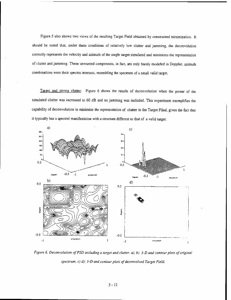
Figure 5 also shows two views of the resulting Target Field obtained by constrained minimization. It

should be noted that, under these conditions of relatively low clutter and jamming, the deconvolution

correctly represents the velocity and azimuth of the single target simulated and minimizes the representation

of clutter and jamming. These unwanted components, in fact, are only barely modeled in Doppler, azimuth

combinations were their spectra intersect, resembling the spectrum of a small valid target.

Target and strong clutter: Figure 6 shows the results of deconvolution when the power of the

simulated clutter was increased to 60 dB and no jamming was included. This experiment exemplifies the

capability of deconvolution to minimize the representation of clutter in the Target Filed, given the fact that

it typically has a spectral manifestation with a structure different to that of a valid target.

c)

d) 0.5

-0.5

Figure 6. Deconvolution of PSD including a target and clutter, a), b) 3-D and contour plots of original

spectrum, c) d): 3-D and contour plots of deconvolved Target Field.

5-12

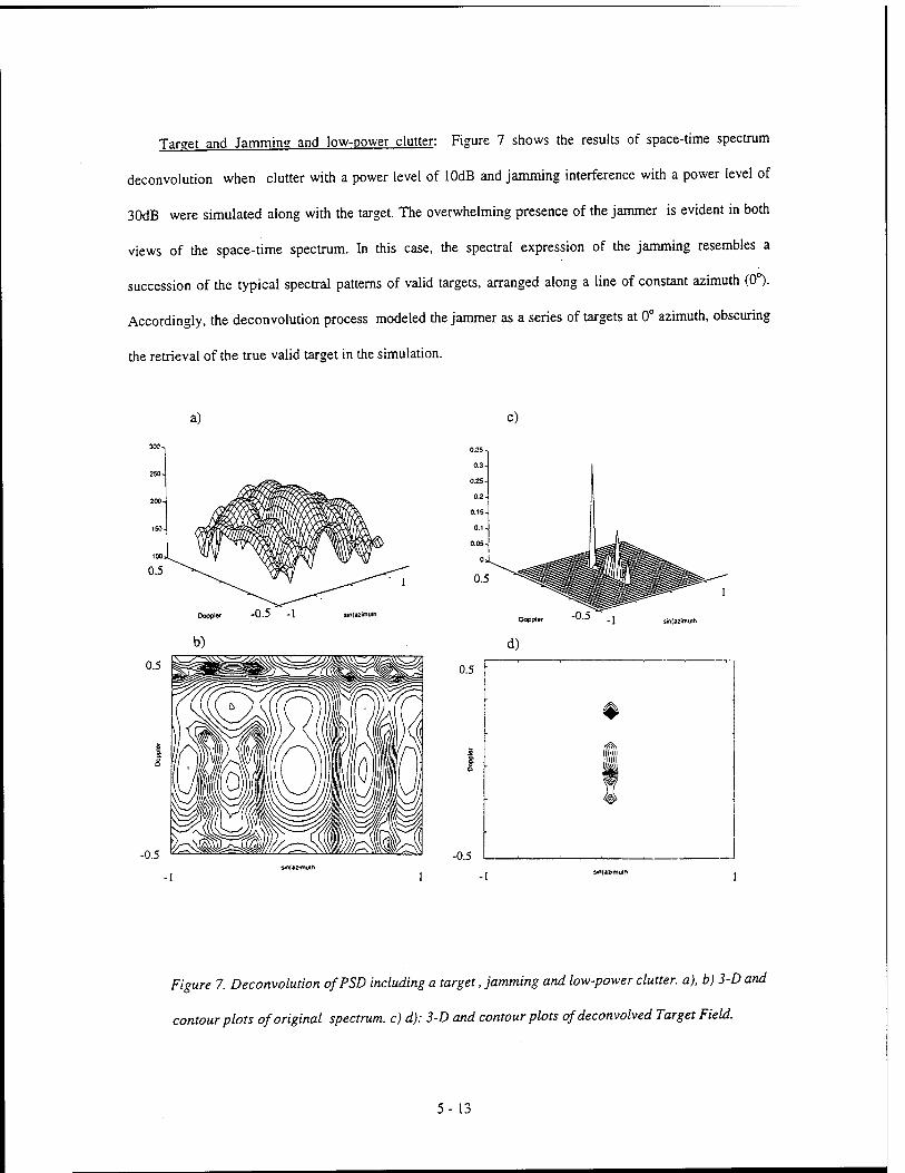
Target and Jamming and low-power clutter: Figure 7 shows the results of space-time spectrum

deconvolution when clutter with a power level of lOdB and jamming interference with a power level of

30dB were simulated along with the target. The overwhelming presence of the jammer is evident in both

views of the space-time spectrum. In this case, the spectral expression of the jamming resembles a

succession of the typical spectral patterns of valid targets, arranged along a line of constant azimuth (0°).

Accordingly, the deconvolution process modeled the jammer as a series of targets at 0° azimuth, obscuring

the retrieval of the true valid target in the simulation.

a)

-0.5 -1

0.5

-0.5

-I

C)

d)

Figure 7. Deconvolution of PSD including a target, jamming and low-power clutter, a), b) 3-D and

contour plots of original spectrum, c) d): 3-D and contour plots of deconvolved Target Field.

5- 13

* Results from real radar data: In order to verify the validity of the deconvolution method to retrieve

an accurate representation of the Doppler and azimuth of targets sensed through a real radar system, some

files from CREST Data Library have been processed. Real data were also used to confirm the observations

regarding the decreased sensitivity of the deconvolution process to clutter components of the space-time

spectrum.

Radar Data including a moving target simulator and IDPCA clutter: The following two experiments

show the results of constrained minimization deconvolution on space-time spectra of data collected

through the Radar Surveillance Technology Experimental Radar (RSTER) using the Inverse Displacement

Phase Center Array (IDPCA) at WSMR, New Mexico. Although the Array is physically at a fixed location,

the sequencing of the transmitted pulses in the IDPCA produces clutter returns equivalent to those sensed

by a moving antenna array. The Internal Test Target Generator in the RSTER was used to generate a target

signal in the record.

t36preöivi.CPt6 - IOPCA cluiter * FiSTER internal target generator Deconvolved. From i38pi<?Ütvl,CPI6 - processed w< Vemi-

c)

-0.5 -1

0.5

-0.5

/ Deconvolved: From tGSpreOlv 1.CPI6 - processed w kern]- S

#' ^ ' |

•IP ®

1

0 j

•4f !

Figure 8. Deconvolution of file t38pre01v.cpi6.mat. a), b) Original spectrum, c) d): Target Field.

5- 14

Figure 8 shows the original space-time spectrum and the deconvolved Target Field for data file

t38pre01vl.cpi6.mat. Here again, the original 256 by 256 space-time spectrum had to be downsampled to

32 by 32 to reduce the computational load of the solution. The spectral manifestation of the target is

discernible in the original space-time spectrum, but it is much more clear and localizable in the deconvolved

Target Field. There is virtually no evidence of a "clutter ridge" in the deconvolved Target Field. Figure 9

shows the results for a similar data file: t38-04vl.cpil.mat. Here the deconvolved Target Field is almost

exclusively defined by a non-zero target element, corresponding to the identifiable Doppler and azimuth of

the discernible target in the original space-time spectrum, with no representation of clutter.

Doppler

d)

sinfarimuih

- -

■

o

o"

-

■ o> \

a. o O

o 4fr o

O

o O

O 1 1

- 0 1

o J

0.5 o

Figure 9. Deconvolution of file t38-04vl.cpil.mat. a), b) Original spectrum, c) d): Target Field.

5- 15

The final example of deconvolution results from real data, shown in Figure 10, illustrates the level of

resistance of the deconvolution process to represent unwanted spectral components that do not conform to

the pattern of valid targets. The file, mmit003vl.cpil.mat, does not contain targets. It only contains "Hot

clutter" and light effects of a jammer, which have already been mitigated in the original space-time

spectrum. The results of constrained minimization deconvolution show a Target Field comprised of several

disorganized and very low-power components (the heights of the elements in the 3-D Target Field plot are

much smaller than those of targets in Figures 8 and 9.)

a) c)

Doppter sin(azimuth Doppfer -0.5 -1

b) 0.5

-0.5

-1 sin(azimuth

d)

0.5

b>

-0.5

O

♦* >

<@>

V -^ku e£s^.

< «

Figure 10. Deconvolution of file mmit003vl.cpil.mat. a), b) Original spectrum, c) d): Target Field.

5-16

Discussion

The results of constrained minimization deconvolution shown in the previous section confirm the

potential of this technique to:

a) Accurately model the presence of valid targets in the Target Field, clearly defining their azimuth

and their velocity, as represented by their Doppler frequency.

b) Provide only a limited representation of space-time spectrum components that do not conform to

the spectral patterns of valid targets, such as clutter.

It should be noted that the above experiments were carried out on space-time spectra downsampled

from their original 256 by 256 size to a reduced size of 32 by 32. This was done to bring the amounts of

storage and processing cycles involved to levels manageable by the system used for this project. The impact

of this simplification was less pronounced in the synthetic data experiments, where the number of antenna

elements, N, and the number of pulses per CPI, M, were both set at a value of six. It is interesting to note

that, for the purpose of deconvolution, the wider sidelobes in Doppler and azimuth that result from these

low values of N and M actually contribute to a good definition of the target spectral pattern in a

downsampled spectrum (K = 32). In contrast, spectra of real space-time snapshots obtained from the

CREST Data Library, recorded using N = 14 and M=16, experienced significant loss of detail through

downsampling, relative to the size of the lobes of the target spectral pattern. These limitations in both the

spectra under analysis and the impulse response used to form the H matrix required for the deconvolution

influenced the appearance of spurious non-zero values around the main components of the recovered Target

Fields.

The capability of the constrained minimization deconvolution to partially avoid the representation of

clutter was evidenced with both synthetic and real (IDPCA) clutter. This feature of the process is attributed

to the fact that the spectral manifestation of clutter is, in general, different from that of a valid target, which

is the one model that is being used for the reconstruction of the Target Field. On the other hand,

experiments involving synthetic jamming showed that the characteristic spectral pattern of barrage

5-17

jamming, spanning all frequencies along a single azimuth line, is interpreted by the deconvolution process

as the superposition of a series of targets with different velocities but lined up in a single angle.

While the deconvolution process does not appear to be able to discard jamming interference in the

reconstruction of the Target Field, its ability to accentuate the presence of valid targets and significantly

reduce the representation of clutter makes it suitable for its integration to partial adaptive algorithms that

excel in removing uni-directional jamming interference {8}. Specifically, spectral deconvolution could be

proposed as post-processing to follow standard beamforming techniques (adaptation in space only).

In considering the merits and potential of this new form of space-time radar data, it must be kept in

mind that this approach attempts to make an efficient use of the combined features in space and time of

data samples captured in a single space-time snapshot. This is in sharp contrast with most fully- or

partially-adaptive space-time processing methods for airborne radar {1}, {3}, {4}. In most of those

approaches the required knowledge about the interference and the target is made accessible by resorting to

the processing of augmented sets of data. For example, the estimation of the interference covariance matrix

Ru, used for the definition of the STAP weight vector that is appropriate for a single space-time snapshot

requires the processing of a number of snapshots "surrounding" the snapshot under study. This "Sample

Support" around the snapshot of interest may involve 2MN to 5MN auxiliary snapshots, each containing

MN space-time samples, under the assumption that the interference is effectively stationary. So, calculation

of a single weight vector, optimized for a specific combination of range, expected target Doppler frequency

and expected azimuth may require manipulation of a matrix Ru of size (MN)3 by (MN)3, in the fully

adaptive case {!}. Additionally, in the absence of a priori knowledge about the expected velocity and

azimuth of the target or targets, a number of different weight vectors need to be calculated and applied to

each space-time snapshot under study, to explore the possibility of finding a target in each Doppler /

azimuth cell of interest within the whole space-time spectrum.

In the context described above, it may be suggested that this new approach to the detection of relevant

targets in space-time radar data may be used, after standard adaptive beamforming to minimize the effects

5-18

of barrage jamming, to indicate the Doppler / azimuth combinations that may contain a target, if any.

Since the process of deconvolution may be carried simultaneously with any of the other fully- or partially-

adaptive STAP methods, this form of preselection of Doppler / Azimuth cells to study could expedite the

determination of presence or absence of a target in a given space-time snapshot.

Conclusions

This report has presented an exploration into the proposition of an alternative approach to the

definition of targets from space-time radar data. Most of the current space-time adaptive processing

methods concentrate in the development of multidimensional filters aimed at establishing nulls in the

areas of the space-time spectrum where the interferences lie. In order to achieve this goal extensive

knowledge about the interference type is needed, which is ordinarily estimated from additional data. In

contrast, the proposed deconvolution approach is based on the knowledge available about the space-time

spectral manifestation of a valid target, minimizing the representation of some forms of interference, such

as clutter, precisely because their spectral manifestation does not conform to the model sought (the spectral

pattern associated with a valid target). The shift of the focus in this alternative approach, from finding out

and de-emphasizing the interference, to finding out and emphasizing the target prompts to the potential

application of space-time spectral deconvolution as a parallel method to other STAP algorithms, within a

comprehensive detection system.

In this project an implementation for the deconvolution of discrete space-time radar spectra was

proposed. This implementation is developed as the constrained minimization of the norm of the difference

between the two sides of the equality relating the abstract 'Target Field" and the space-time spectrum of

radar data contained in a single snapshot. The proposed implementation was used to prove the feasibility

and potential of the deconvolution concept with both synthetic and real data. In both cases the method

showed the ability to properly represent valid targets while significantly de-emphasizing clutter. On the

other hand, the method was only able to de-emphasize the representation of jamming interference of low

power. Accordingly, it was suggested that for a realistic scenario an adaptive beamforming pre-processing

5-19

block aimed at canceling jamming would greatly benefit the performance of the deconvolution approach. It

is important to note, however, that while jamming interference may be very powerful and overwhelm a

target detection system, it is still a "one-dimensional" interference (single azimuth). On the other hand,

space-time deconvolution appears to be useful against some forms of interference that are truly two-

dimensional in nature, such as the clutter ridges that appear in spectral configurations (e.g. diagonals) that

effectively span a full range of Doppler frequencies and azimuth values.

References:

1. Ward, "Space-Time Adaptive Processing for Airborne Radar", Technical Report # 1015, Lincoln

Laboratory, MIT, Lexington Massachusetts, December 1994.

2. Y. Seliktar, D. Williams and J. McClellan, "Evaluation of Partially Adaptive STAP Algorithms

on the Mountain Top Data Set", ICASSP 96 (pre-print).

3. Wang and L. Cai, "On adaptive Spatio-Temporal Processing for Airborne Surveillance Radar

Systems", IEEE Transactions on Aerospace and Electronic Systems, Vol. 30, No. 3, July, 1994,

pp. 660 - 669.

4. C. Barile, T. P. Guella and D. Lamensdorf, " Adaptive Antenna Space-Time Processing

Techniques to Suppress Platform Scattered Clutter for Airborne Radar", IEEE Transactions on

Aerospace and Electronic Systems, Vol. 31, No. 1, January 1995, pp. 382 - 389.

5. Skolnik (ed.), "Radar Handbook, 2nd. Edition", McGraw-Hill Publishing Co., 1990.

6. Lawson and R. Hanson, " Solving Least Squares Problems", Prentice-Hall Series in Automatic

Computation, 1974.

7. Titi, "An overview of the ARPA/NAVY Mountaintop Program," 1994 IEEE Long Island Section

Adaptive Antenna Systems Symposium, Melville, New York, November 7-8, 1994.

8. Compton, Jr., "Adaptive Antennas, Concepts and Performance", Prentice-Hall, 1988

5-20

THE USE OF WAVELETS AND NEURAL NETWORKS IN DATA COMPRESSION, DATA FUSION AND THEIR EFFECTS ON TARGET IDENTIFICATION

LARRYA.BEARDSLEY INSTRUCTOR OF MATHEMATICS DEPARTMENT OF MATHEMATICS

UNIVERSITY OF TEXAS 26th & SPEEDWAY

AUSTIN, TX

Final Report for: Summer Faculy Research Program

Wright Laboratory Armament Directorate

Eglin Air Force Base, Florida



and

Wright Laboratory

September 1996

6-1

THE USE OF WAVELETS AND NEURAL NETWORKS IN DATA COMPRESSION AND FUSION WITH RESPECT TO TARGET IDENTIFICATION

Larry A. Beardsley Instructor of Mathematics

Department of Mathematics University of Texas

Abstract

The usefulness of wavelets in digital and signal processing has been widely accepted and appreciated for the

past several years. Also, the need for data compression as well as the ability to train networks via radial basis

functions has been known for the past decade. This research was conducted for the purpose to ascertain the benefits

of using wavelets for data compression followed by the use of a radial basis function to determine if data fusion in the

context of infared and passive millimeter wave imaging can benefit the identificatiion of potential targets as well as

discriminate between a non-target. The study showed that data compression can be attained while retaining a high

percentage of image characteristics of a target. Also, it is conjectured that data fusion most likely enhances target

identification. However, further study needs to be udertaken to determine under what conditions data fusion is most

successful. Finally, further investigation needs to be done to determine how well a non-target can be discriminated

from a non-target using neural networks.

6-2

THE USE OF WAVELETS AND NEURAL NETWORKS IN DATA COMPRESSION AND DATA FUSION WITH RESPECT TO TARGET IDENTIFICATION

LARRYA.BEARDSLEY

Introduction

In the recent past, the need for data compression has been recognized in many different applications. One

of the most well-known uses of data compression is in its value to fingerprinting. As of June, 1994, the FBI had about

30 million sets of fingerprints [ 5]. This number has substantially increased. These need to be digitized. For example,

when a thief is apprehended, fingerprints are recorded electronically. A central computer looks for a match. Until the

early 1990's, this process was time consuming and this would be costly to the chances of apprehending of the criminal

in time that could be valuable. In the beginning, it was expected that older Fourier methods would succeed here.

However, with a compression ratio of 20:1, the fingerprint ridges could not be easily followed due to the fact that lines

were broken between one eight-by-eight square and the next. Also, the short-timed Fourier transform introduced too

much blocking. With the used of wavelets, the image can be compressed at the given ratio of 20:1 with little loss of

information.

With the above applications and even earlier ones, it was conjectured by prominent individuals in academia,

industry, and the defense agencies, that there may be widespread advantages to military applications. Since time is of

the essence when imaging a military target with either passive millimeter wave or infared or both, the less the amount

of data to be processed to obtain virtually the same target, the better. Since the advent of the Coiflet and Daubechie

wavelet, great work has been accomplished in many applications, and data compression is one of these.

For the past year, the effect of using wavelets in military applications has been studied. This study was

undertaken to determine if wavelets were beneficial in target identification with less data. Also, later in the research

period, the study of neural nets and radial basis functions was underaken to see how it benefited in target recognition

using the two methods of imaging, passive milliter wave and infared. No strong results are presented in this paper with

respect to this last venture due to time constraints. However, the value of the use of neural nets to train for target and

non-target is not to be minimized. A detailed summary report of results of compression of images and the effects of

data fusion on the given images using PCNN is to be presented to the laboratory along with this final report. Due to the

classification of the images and the number of them, they are not included in this report. Also, more detailed

suggestions are included in that follow-up report.

Methodology

Several military targets were provided by the laboratory. These targets were in the form of what is commonly

called "raw format" or lif format". The "t'rf" formatted files could be opened using microsoft word. However, the wavelet

analysis could not be performed in this format. Yet, the raw format could be manipulated using matlab and a wavelet

6-3

toolbox to perform both imaging and data compression. Also, results could be derived using matlab programming to

determine the percentage of the image retained as well as generating histograms of the wavelet coifficients which in

turn gave useful information. Also, programming was done to decompress the data. The results of data compression

were very positive yielding high compression ratios while retaining the "energy" of the given picture; that is, the image

was virtually the same after data compression.

The last aspect of the study took place with only a few weeks of the researcher's tenure at the laboratory.

So, conclusive results were not found. However, using a method called PCCN, "pulse-coupled neural networks", to

segment the data, it is conjectured that PCCN can be used in the fusion of the two methods of imaging yielding

enhanced results in particular cases. Under what conditions, fusion is favorable needs to be studied as well as the

accuracy that target and non-target can be discriminated.

The Experiment

Original infared and mmw images were compressed using both the Daubechie2 and Daubechie6 wavelet

to compress the entire images. Then, PCNN was run on the entire image. Outlines of the regions of interest (ROI) of

possible targets were generated. Then a wavelet histogram routine was used to find the 50 (or 25, or other depending

on what was called for) on the largest coefficients. A window was created around the region of interest. Then, an RBF

algorithm "was to be used" to train a radial basis function using the given coefficients or the the wavelet histograms.

The next step was to do this for all N-1 histograms for training. Then, results were to be kept track of based on

probably of hit P(Hit) and P(miss).

6-4

THE USE OF WAVELETS AND NEURAL NETWORKS IN DATA COMPRESSION AND DATA FUSION WITH RESPECT TO TARGET IDENTIFICATION

The appearance of wavelets in mathematics is not so recent in mathematics but it is fairly recent in its

application to engineering, in particular to digital signal processing. The word wavelet or "ondelette" was first known to

have been used by the French researchers, Morlet [1}and Grossman [ 2 ], [3], in the early 1980's. However, the

existence of wavelet-like functions has been known since the early part of the 20th century, the first examples being

the Haar wavelet and the Littlewood-Payley wavelet. Many of the ideas formulated using wavelets have their origins in

work in subband coding in engineering, coherent states and renormalization group theory in physics and the study of

Calderon-Zygmund operators in mathematics. However, it was not until recently that the unifying concepts necessary

for a general understanding of wavelets were provided by researchers such as [5] Stromberg, Meyer, Mallat,

Daubechies, and Lemarie. Since that time, the growth of applications of wavelets has been colossal with numerous

authors contributing significantly to the research.

To give the reader an appreciation for how wavelets play a role in data compression, it seems appropriate

that a short introduction to wavelets be given in this paper.

The wavelet transform is a tool that cuts up data, functions or operators into different frequency components,

and studies each component with a resolution matched to its scale. For example, in signal analysis, the wavelet

transform yields a time history in terms of its frequency components. In this one respect, the wavelet transofrm

performs in much the same way as the Fourier transform. The Fourier transform extracts from the signal details of the

frequency content, but loses all information on the location of a particular frequency within the signal. A partial solution

is attempted by windowing the signal and then taking its Fourier transform. The problem with windowing is that the

slice of the signal that is extracted is always the same length. As a result, the slice or number of data points used to

resolve a high-frequency component is the same as the number used to resolve a low-frequency component. The

wavelet transform's solution to this is that it adapts the width of its time slice according to the frequency components

being extracted. For example, for a windowed Fourier transform expressed as

Crf)(w,t)= J7(s)g(*-Oe**ds,

then the corresponding wavelet transform is

(t-bs

(r"f)(a,b)= J/(Oq> dt

where the position of the slice of the signal that the wavelet samples in time is controlled by V and the extent of the

slice by the parameter 'a". Wavelets are being used in signal processing to develop best basis methods for signal

compression and signal characterization.

6-5

THE CONSTRUCTION OF WAVELETS AND THE RELATION TO DATA COMPRESSION

The construction of wavelets begins with vectors. We begin with the concept that every two-dimensional

vector (x,y) is a combination of the basis vectors (1,0) and (0,1). For example, the vector (4,3) can be obtained by

multiplying the first basis vector, (1,0) by 4 and the second basis vector, (0,1), by 3. In a like manner, all possible

vectors can be obtained by using the same two basis vectors. The basis vectors are not unique, but the number of

basis vectors for a given dimension, "n", must be also be "n". The best bases have another valuable property,

orthogonality. For example, the standard basis for R2 includes the vectors (0,1) and (1,0), and of course their dot

product is 0.

Considering four dimensions where we take the four components (x, , x2, x3, x4 ) as the strengths of the

signal, if the signal is x = (1,1,1,1), the tone is steady whereas if x = (1,2,4,8), the volume is increasing. An easy way

to send a signal x is to give its four components. You are then using the basis for R4 with basis vectors (1,0,0,0),

(0,1,0,0), (0,0,1,0), and (0,0,0,1), and the numbers x,, x2, Xj and x4 are sent. You may question how this could be

less than optimal. The answer depends on the signal being transmitted.

Compression discards basis vectors that are absent or barely present in a signal. When the vectors

represent different frequencies, the Fourier basis, high frequencies can often be discarded. With the standard basis,

the vector (0,0,0,1) can be discarded, for example when the fourth vector is not used. It was novel in the early 1900's

to devise a basis that included the constant, or scaling vector, (1,1,1,1) and the second basis vector (1,1,-1,-1), up

once and down once. Alfred Haar, the German mathematician, completed a perpendicular baisis in 1910 by dilation

and translation (ie. squeezing and shifting). He squeezed the vector (1,1,-1,-1) to produce the third vector (1,-1,0,0).

Then, he shifted the third vector by two time intervals to produce the fourth vector (0,0,1,-1). These basis vectors are

the columns of the Haar matrix.

H4 =

To find the amplitudes for longer signals, averages and differences are used. The averages move up in a

pyramid to be averaged again. The differences give the fine details at each level. Compression works by ignoring

what the eye cannot see and the ear cannot hear. So, for example, when a signal changes quickly, it is considered

unimportant; when a signal is almost steady, the signal may not be transmitted. The concept being developed here is

that of what is called multiresolution. We see a signal at multiple scales, fine, medium, and coarse. The signals are

resolved at each scale by details and averages.

1 1 1 0"

1 1 -1 0

1 -1 O 1

1 -1 0 1

6-6

HOW MULTIRESOLUTIONAL ANALYSIS WORKS?

Before undertaking how multiresolutional analysis works, it may be helpful to first look at how to develop a

multilevel representation of a function. The goal of multiresolution analysis is to develop representations of a function

f(x) at various levels of resolution. We achieve this by expanding the given function in terms of basis functions <t>(x)

which can be scaled to give multiple resolutions of the original function. In order to develop a multilevel representation

of a function in L2(R) we seek a sequence of embedded subspaces V, such that

{0}...cV,cVDcV1cV,..cL!(R)

with the following properties:

(a) M j eZ V j is dense in L2(R). (where Z is the set of integers.)

(b) f|;eZVj={0}

(c) The embedded subspaces are related by a scaling law

g(x)eVi «.g(2x)eVM

(d) Each subspace is spanned by integer translates of a single function g(x) such that

g(x)€ V0 og(x + 1)eV0

We also seek a scaling function tfx) e V0 such that its integer translatges {tfx - k), k e Z} from a Riesz basis for the space V0. Then <J>(2x - k) form a basis for V, (Scaling by powers other than two is possible but is not discussed here.) Therefore,

V0 = span{ <|>(x - k), k e Z} V, = span{(K2x-k),keZ}

Since the space V0 lies within the space V,, we can express any function in V0 in terms of the basis functions

of V,. In particular, <t»(x) = ^ ak 0(2* - k) in which a k, ke Z is a square summable sequence. (*)

We will refer to equation (•) as the dilation equation. The dilation equation is often referred to as the refinement equation or the scaling relation.

If we now define 4 mk(x) = 2m'2 4>(2mx- k), then 4 Jx), keZ forms a Riesz basis for the space V.. The dilation parameter m will bae called the scale.

An example using the box function as a basis (commonly know as the Haar basis).

6-7

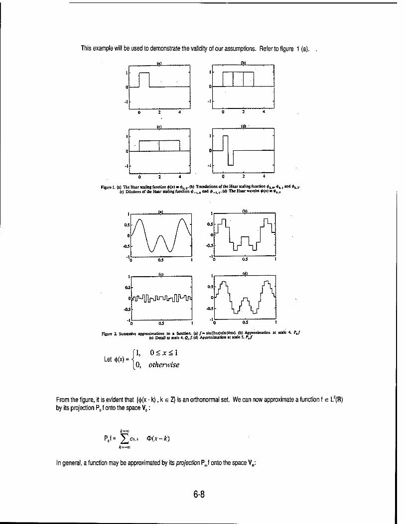
This example will be used to demonstrate the validity of our assumptions. Refer to figure 1 (a).

i •

fa)

•

■ ■

(b)

•

to I - I—I

<<n -

■

Figure 1. (a) The Haar seating function «V(x) ■ *o o- 0* Translation» of the Haar sealing function #„.,, *„,, and ^ r

<c) DilationsoftheHaarscalingfiinction«.lt0and»i.,.,.{<« The Haar wavelet Wx) H iff,,.

Figure Z Successive approximations to a function. (a)/-sin(2nx)sin(4itx). (b) Approximation at scale 4. TJ (c) Detail at scale 4. Q.f. <d) Approximation at scale 5, P,f

Let <(>(x): [1, 0<x<l

[O, otherwise

From the figure, it is evident that {<j>(x - k), k e Z} is an orthonormal set. We can now approximate a function f e L2(R) by its projection P0 f onto the space V0:

A=oo

P0f= ]Tco,* ®(x-k) k=-ca

In general, a function may be approximated by its projection Prof onto the space Vm:

6-8

£=oo

Pmf=FV= !/"•* *«■*(*) k=-oo

Infact Pmf approaches f as m -> °o

Figures 2 on p. 7 and Figure 3 below show two approximations to a function at consecutive scales. Note that the box function satisfies the dilation equation with coefficients a0 = a, = 1, and <|>(x) = <|>(2x) + <J>(2x -1), and from this we can see that

w . , , _, m i ■ l

0

•1 ■'

Figure 3. (a) Haar leafing (unction, (b) Haar wavelet, fc) Daubechiet D4 scaling function. <d) Daubechies D4 wavelet. (e) DaubecbiaD6icalin» function.(f) DtobechiaD6wavdct.(|) BatÜe-Larariescalinsfuocl»n,(h) Batäe-Lemarie

wavelet

V,cV,cV,

This example shows that the box function can be used to develop a sequence of embedded spaces with each space spanned by the translates of the box function at that scale.

Now , multiresolution decomposition takes the expansion coefficients cmk of an approximation Pm f, to a function at scale m and decomposes them into

(1) the expansion coefficients, c„,Ui of the approximation P„,, f at the next coarser scale m -1,

6-9

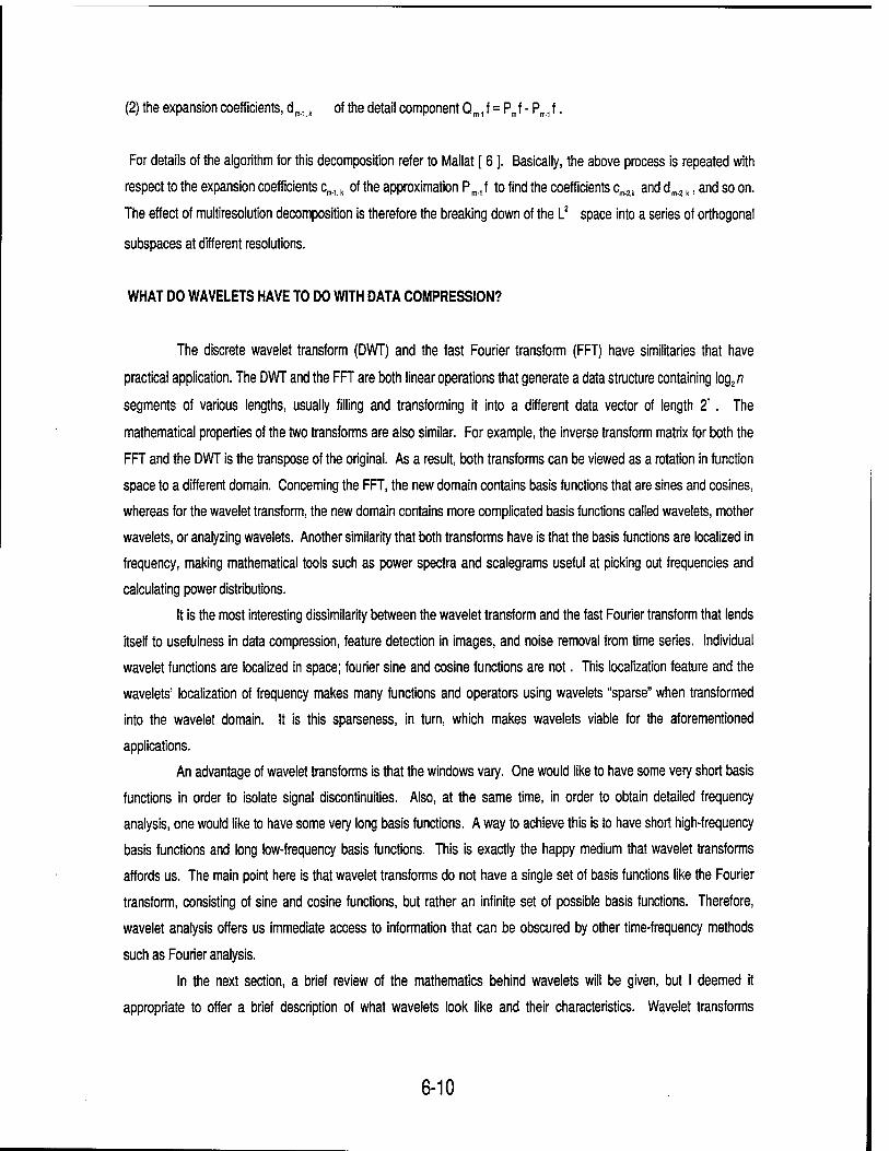
(2) the expansion coefficients, dm., k of the detail component Qm.,f = Pmf - P^f.

For details of the algorithm for this decomposition refer to Mallat [ 6 ]. Basically, the above process is repeated with

respect to the expansion coefficients cm.u of the approximation Pm.,f to find the coefficients c^ and dm.ak, and so on.

The effect of multiresolution decomposition is therefore the breaking down of the L2 space into a series of orthogonal

subspaces at different resolutions.

WHAT DO WAVELETS HAVE TO DO WITH DATA COMPRESSION?

The discrete wavelet transform (DWT) and the fast Fourier transform (FFT) have similitaries that have

practical application. The DWT and the FF are both linear operations that generate a data structure containing log2n

segments of various lengths, usually filling and transforming it into a different data vector of length 2". The

mathematical properties of the two transforms are also similar. For example, the inverse transform matrix for both the

FFT and the DWT is the transpose of the original. As a result, both transforms can be viewed as a rotation in function

space to a different domain. Concerning the FFT, the new domain contains basis functions that are sines and cosines,

whereas for the wavelet transform, the new domain contains more complicated basis functions called wavelets, mother

wavelets, or analyzing wavelets. Another similarity that both transforms have is that the basis functions are localized in

frequency, making mathematical tools such as power spectra and scalegrams useful at picking out frequencies and

calculating power distributions.

It is the most interesting dissimilarity between the wavelet transform and the fast Fourier transform that lends

itself to usefulness in data compression, feature detection in images, and noise removal from time series. Individual

wavelet functions are localized in space; fourier sine and cosine functions are not. This localization feature and the

wavelets' localization of frequency makes many functions and operators using wavelets "sparse" when transformed

into the wavelet domain. It is this sparseness, in turn, which makes wavelets viable for the aforementioned

applications.

An advantage of wavelet transforms is that the windows vary. One would like to have some very short basis

functions in order to isolate signal discontinuities. Also, at the same time, in order to obtain detailed frequency

analysis, one would like to have some very long basis functions. A way to achieve this is to have short high-frequency

basis functions and long low-frequency basis functions. This is exactly the happy medium that wavelet transforms

affords us. The main point here is that wavelet transforms do not have a single set of basis functions like the Fourier

transform, consisting of sine and cosine functions, but rather an infinite set of possible basis functions. Therefore,

wavelet analysis offers us immediate access to information that can be obscured by other time-frequency methods

such as Fourier analysis.

In the next section, a brief review of the mathematics behind wavelets will be given, but I deemed it

appropriate to offer a brief description of what wavelets look like and their characteristics. Wavelet transforms

6-10

comprise an infinite set, and different wavelet families yield different trade-offs between how compactly the basis

functions are localized in space and how smooth they are. Many of the wavelet bases have fractal structure of which

the Daubechies wavelet family is an example. Within each family of wavelets are wavelet subclasses distinguished by

the number of coefficients and by the level of iteration. This is an extra set of mathematical relationships which the

coefficients must satisfy and is directly related to the number of coefficients. [ 7 ]

The key to the wavelet analysis procedure is to adopt a wavelet prototype function, called a mother wavelet.

Temporal analysis is performed with a contracted, high-frequency version of the protype wavelet, while frequency

analysis is performed with a dilated, low-frequency version of the same wavelet. Since the original signal or function

can be represented in terms of a wavelet expansion (using coefficients in a linear combination of the wavelet functions,

data operations can be performed using just the corresponding wavelet coefficients. If you desire further to choose the

wavelets best adapted to your data or truncate the coefficients below a threshold, your data are sparsely represented.

It is this sparse coding that makes wavelets an excellent tool in the field of data compression.

HOW ARE FILTER COEFFICIENTS DERIVED FROM GENERALIZED SCALING FUNCTIONS AND WAVELETS?

From a heuristic standpoint to aid in a pedagogical environment, the Haar scaling function and Haar wavelet

previously described are very useful. However, from an applied standpoint, particularly to digital signal processing, the

Haar wavelet is not very useful. Their graphs are made from flat pieces consisting of 1's, O's, and -1's, and

approximation to most signals is poor at best. Many flat pieces are needed to represent even a sloping line to decent

accuracy. The Haar basis will not give compression ratios desired such as 20:1 minimally or 100:1. The key to the

problem is a better basis.

Actually, the Haar basis and scaling function described earlier are special cases of a more general class of

functions. In general, a scaling function, <D (x), is the solution to a dilation equation of the form

<D(x) = £ak ®(Sx-k) (1)

A good choice of the dilation factor is S = 2, in which case the equation becomes

4>(;c)= £ak <S>(2x-k) (2) k=-<o

The constant coefficients a, are called filter coefficients and it is often the case that only a finite number of these are

non-zero. The filter coefficients are derived by imposing conditions on the scaling function, 4>0). One condition is

that the scaling function and its translates should form an orthonormal set; that is,

6-11

j<DO0<D(x + />fc = 6,^ t eZ (3)

ri, /=o where 5 0 it. ,

[0, otherwise

A wavelet, *F (x), is orthogonal to the scaling function and is defined by

*(x)= S^'^-I-K *(2*-*) (4)

where N is an even integer. This definition satisfies orthogonality since

4=a> i=eo

<*(*),¥(*)> = L £ak 4(2*-*) £(-1) ' aN-i-1 <t>(2x-I) dx £=-» £=-oo

= 0.

The set of coefficients {ak} and {(-1)kaN.1.K> are said to form a pair of quadrature mirror filters.

Figure 3 depicts the Haar scaling function and Haar wavelet, Daubechies 4 scaling function and Daubechies 4

wavelet, Daubechies 6 scaling function and Daubechies 6 wavelet, and the Coiflet 2 scaling function and Coiflet 2

wavelet respectively. These were obtained by using different sets of filter coefficients to solve equations 3 and 4

above.

Now for the derivation of the coifficients. In order for the scaling function to provide a useful basis for

functional analysis, it should satisfy useful properties which lead to corresponding conditions on the filter coefficients.

These properties are:

(I) To uniquely define all scaling functions of a given shape, the area under the scaling function is normalized to unity;

that is,

00

[*(*)& =1. (4') —00

Also, the fact that the scaling function has a non-vanishing integral forces the sum of the filter coefficients to be equal

i=oo

to 2; that is, V a k = 0. (If this is not obvious, employ the "trick" of multiplying the scaling function 4(x) by 2 and t=-00

integrating by 2 to obtain

6-12

a> £=oo

2\®(x)dx = 2 I ^ak <H(2x-*)

£=oo » = Xa* J*(2*-*y(2*-*)

£=-oo _oo

£=a>

=> 2>>-2. (5)

£=-oo

£=oo

The uniqueness of #0) is guaranteed by ]Tak = 2. However, a smooth solution does not necessarily follow. £=-«>

As an example, let c0 = 2 with <D(x) = 8 (x). Then 8 (x) = 28 (2x), and yet the delta function is not smooth.

For a scaling function to be orthogonal to its integer translates, the filter coefficients must satisfy the additional

CO

requirement that J <D(x)0(x + £)dx = 8 0_ / I e Z -co

Jt=co

This forces the condition £ ^t + 2, = 2 8 0 g _ / e Z (6) £=-oo

To determine a unique set of filter coefficients, one more condition other than (5) and (6) needs to be satisfied. In an N

coefficient system, the two equations yield a total of N/2 +1 equations. For a unique solution, another N/2 -1

equations are necessary. To obtain the remaining equations, it was discovered by Daubechies [ 4] that we can

require the scaling function to be able to exactly represent polymonials of order up to, but not greater than p.

Enforcement of this requirement results in the compactly supported wavelets developed by Daubechies. This

requirement for approximation of order p is that any function of the form

f(x) = a,+ a,x+ a/ + a,x" + •• +a,, (7) £=oo

can be exactly represented by an expansion of the form f(x)= ^ a „*(*-*). (8)

Another way of saying this is that the polynomials 1,x,..., x1* are linear combinations of the translates,

<E>0 - k). This now may be translated as a condition on the wavelet. Taking the inner product of the equation in (8)

with \j/(;c) yields

</(*),¥(*)> = £ a k <$>(*-*), ¥(*)> = 0. £=-oo

Using this result with (7) and (8), we arrive at oo oo °o

a„ f¥(*)<& +a, $V(x)xdx + a2+ -- + \, j^Wx^dx. -oo-oo -oo

Since this identity is valid for all ^ (j = 0,1,2,..., p-1), choosing a,= 1 and letting all other a, = 0

6-13

yields f^(x)X dx = 0, ^ = 0,1,2 p-1 (9)

So, the first p moments of the wavelet must be zero.. To determine the constraints this places on the filter coefficients,

substitute equation (4) into (9). From this, it can be shown that

£ (-1)kay==0,/=0,1,2 p-1 (10)

It was shown earlier that equation (10) must yield n/2 -1 new equations. Now, the equation obtained by letting I = 0 is

redundant since it may be obtained from

■>j2[equaion(6)]i . o + 4[equation(6)} > o - [equation(5)]2 (11)

Equation (11) yields p-1 new equations which implies from (9) that p = N/2. So, the final conditions on the filter

coefficients is

£ (-1)kakk^=0, £ = 0,1,2 N/2-1 (12) £=-oo

Thus, the filter coefficients {a„k = 1 N -1} for an N coefficient system are uniquely defined by (5), (6), and (12).

The table below gives the coefficients for the Daubechies D$, D6, and D8 wavelet systems. The final problem that has

to be constructed is the actual scaling function O(x) from the fillter coefficients.

Table I. Filters coefficients for Daubechies DN filter where N = 4, 6, and 8 (rounded to nearest ten thousandth).

k D4 D6 D8

0 0.6830 0.4704 0.3258 1 1.11830 1.4144 1.0109 2 0.3170 0.6504 0.8922 3 -0.1830 -0.1909 -0.0396 4 -0.0450 0.2645 5 0.0498 0.0436 6 0.0465 7 -0.0150

6-14

How are the scaling functions constructed?

Generally, scaling functions do not have a closed form solution; rather, they have to be generated recursively

from the dilation equation (2). This equation may be explicitly written as

<DO) = aod>(2x) + a.O(2x -1)+.. .+a» - &(2x - N +1)

Writing this relationship for all integer values x = j, the following set of equations can be generated.

0(0) = aoO(O)

O(l) = ao<t>(2) + a.O(l) + a20)(0)

(J>(2) = aod>(4) + aiO(3) + a2<D(2) + a&(l) + a&(0)

®(N-2) = a«-&(N-l) + as-2®(N-2) + a*-i®(N-3)

<D(JV-l) = a»-.<D(iV-l)

The matrix form of the above can be generated and may be written as M O = <I>.

So, the vector of integer values of the scaling function, <E>, is the eigenvector of M corresponding to the eigenvalue 1.

As in all eigenvalue problems, the solution of the equation

(M-l)O = 0. (13)

is not unique, and therefore a normalizing condition is needed in order to determine a unique eigenvector. In this case

the normalizing condition arises from equation 4'. After some calculation, we obtain

§ 0(i) = 1,ieZ (14) £=-co

Therefore, the values of the scaling function at the integers are given bhy the solution to equation (13) and normalized

by equation (14). So, we have how to find the integer values of Y; the values of

O(x) of the half integers can be found by equation (2). That is,

0(x/2)= J^aMx-k), <15>

So, this process is repeated as many times as necessary to find the values of 0(x) at all dydadic points

{i/2n ,neZ)

How to Calculate the Wavelet Coefficients for a particular Example.

An example: The Daubechies 4 coefficient wavelet system

6-15

We will demonstrate how to use the previous results to construct the D4 (Daubechies 4 coefficient) scaling

function and wavelet.

(1) First construct the filter coefficients.

So, we want to solve equations (5), (6), and (12). The easiest way todo tihis is to include the redundant

equation for £ = 0 in equation (6), which we know is linear, and to exclude the non-linear equation for £ = 1in equation

(12). Therefore, we have

a,+^+^+8, = 2

a02+a,2+a2

2a/=2

-a0 +a,+2a2 -3aj = 0

Now, from the above linear equations, we have:

a^a,. -1/2, a2=3/2-a, ,a,= 1 -a,

Substituting for a 0, ^ , and % in the quadratic equation and solving gives

3±V3 a, = , and from this we find that

1±V3 3 + V3 1 + V3 ■>*ts

4

It is obvious that one set of solutions is the antithesis of the other. That is, if one leads to the scaling function O (x),

then the other will lead to <D (-x). Yet, both equations satisfy the condition of normality, orthonormality and exact

representation of a linear function. The solution that will be adopted is the one with the upper of "plus-minus or minus-

plus" in the above notation.

The values of the scaling function at the integer points are given by equation (13):

Ö0-1 0 0 0 " 0(0)- ■o

dl tfo-i do 0 *G) 0 0 03 flo-i a\ 0(2) 0 0 0 0 flo-i _d>(3)_ 0

From this, we find that O(O) = 0, <D(3) = 0, <t>(2) = _ 1-V3

1 + V3 <I>(1)

6-16

Substituting this into equation (14) yields

m = l±A and <D(2) = ^

Equation (15) then gives us the values of <f?(x) at the half-integers.

2 u w 4

o^=a3<D(2)+a2<D(i)=o

^Uo(2) + 2-^ .2) "" ^ 4

Now, the Mallat [6] transform decomposition algorithm or another can be used to operate on the coefficients

for data compression.

6-17

REFERENCES

1. J. Morlet, G. Arens, I. Fourgeau and D. Giard, Wave propagation and sampling theory',

Geophys., 47,203-236 (1982).

2. J. Morlet, Sampling theory and wave propagation', in Chen (ed.) NATO ASI Series, Issues in

Acoustic Signal/Image Processing and Recognition, Vol. I, Springer, Berlin, 1983, pp. 233-261.

3. A. Grossman and J. Morlet, 'Decomposition of Hardy fuctions into square integrable wavelets of

constant shape', SIAM J. Math, Anal, 15.723-736 (1984).

4. J.O. Stromberg,' A modified Franklin system and higher order spline systems on Rn as

unconditional bases for Hardy spaces', Conf. in Honour of A. Zygmund, Vol. II, Wadsworth Math.

Ser., 1982, pp. 465-493.

5. G. Strang, "Wavelets", American Scientist, 82,250-255, (1994).

6.. S.G. Mallat," A theory for multiresolution signal decomposition: the wavelet decomposition",

IEEE waveletdecomposition",IEEE Transactions on Pattern Analysis and Machine Intelligence,

2(7), 674-693 (1989).

7. I. Daubechies, Ten Lectures on Wavelets, CBMS-NSF Regional Conference Series, SIAM,

Philadelphia, 1992.

6-18

Variable-Width Template Construction for ATR with HRR Data

Raj Bhatnagar Associate professor

ECECS Department

University of Cincinnati Cincinnati, OH 45221

Final Report for: Summer Faculty Research program

Wright Laboratory

Sponsored By: Air Force office of Scientific Research

Boiling Air torce Base, DC

and

Wright Laboratory

September 1996

7- 1

1 Introduction

The research described in this report was conducted with the objective of studying and suggesting ways to improve the performance of Air-to-Ground Target Recognition systems that use High Resolution Radar (HRR) data. Specifically, we worked with the HRR data for five target vehicles.

During the first phase of research we performed a number of investigations with the objective of learning about the nature and characteristics of the HRR data. Our perspective during these studies was to determine the suitability of various types of features for the classification of target vehicles.

The insights provided by these studies led us to hypothesize that ATR performance can potentially be improved if instead of uniform-width templates, sets of variable-width templates are constructed from data. We developed a heuristic search based algorithm for constructing variable- width templates and demonstrated the potential improvement.

In the following sections we first list the results of the studies performed with the data and then outline our algorithm and results for constructing variable-width templates. We also describe a hierarchical attributes based recognition system for which only some preliminary work was initiated during this study.

2 Nature of Data

Our studies were performed using synthetic data generated by the XPATCH system. A brief description of the data is as follows. A transmitted signal containing 100 different frequencies is beamed at the target vehicle and the reflected energy is collected. This reflected energy depends on the shape of the reflection characteristics of the area from which it is reflected. A plot of the reflected energy for the 100 pulses, the (signature), contains information about the characteristics of the reflecting area. The data consists of signatures obtained from every 0.04 degree of each target vehicle. This gives us a 100 x 9000 matrix of complex numbers for each target vehicle and for a fixed elevation angle. We worked with the data for 5 target vehicles. These vehicles were: Ml tank, T-72 tank, School Bus, Fire Truck, and Scud Missile.

3 General Approach

The three phases of the ATR process are: (i) Pre-processing of data; (ii) Data Reduction and Representation; and (iii) Pattern Recognition. In the following, w? discuss the prevalent methods, details of studies performed by us and the results of modifications implemented by us.

3.1 Pre-Processing of Data

Most prevalent methods transform the signatures from frequency domain into time domain using Fourier Transform methods and work with the resulting Range-Profile data. In our studies we used the magnitude part of such Range-Profile data. We also performed a power transform of the data before using it so as to restore the normal distribution of the values that gets altered during the process of computing magnitude of complex numbers. A plot of one range profile is shown in Figure-1. Figure-2 shows the intensity plot for the 9000 range profiles of one target.

7-2

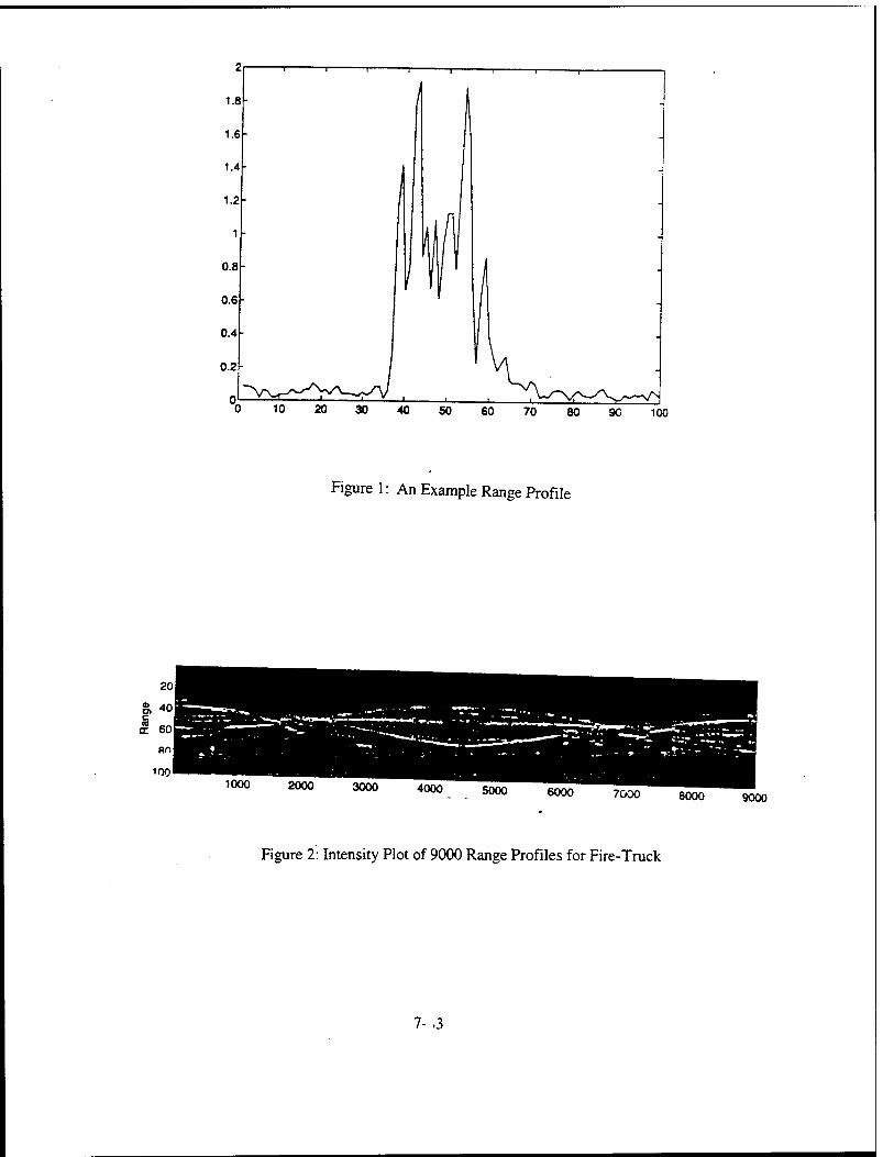
100

Figure 1: An Example Range Profile

1000 ^ **»400°. . 5000 6000 7OD0 8000 9000

Figure 2: Intensity Plot of 9000 Range Profiles for Fire-Truck

7- 3

3.2 Data Reduction and Representation

The data that needs to be stored for each target consists of one array of 100 x 9000 complex numbers for each target, and for each angle of elevation. This is an enormous amount of data. There is a large amount of redundancy in this data which arises due to the fact that signature of a vehicle varies only gradually as we change the rotational and/or the elevation angle.

In current ATR methods, this redundancy is exploited by constructing templates of fixed-sized angular regions around a vehicle. Typically. 180 templates of 2-degree angular width each may be constructed for a vehicle. Within each such template fifty contiguous range-profiles are averaged to obtain the representative template signature. During the recognition stage, a signature is matched to these templates to find the closest template. Figure-3 shows the intensity plot of range profiles for T-72 (for 90-180 degrees region) and also a similar plot for 3-degree templates in this region. Representation of 9000 range profiles for a target by 120 or 180 template signals is significant reduction in the amount of data to be stored.

3.3 Recognition

The Prevalent Method is to determine the distance between the sample (to be classified) range- profile and each of the template signals and find the closest template. Sample is then classified as belonging to the target of the closest template.

4 Preliminary Investigations

We performed a number of investigations for determining the characteristics of the HRR data for the targets. Most of these investigations employed measurement of various information-theoretic quantities for the data sets. A brief description of the investigations and their results is mentioned below.

• Task 1: We computed informational entropy for each range profile for the HRR data for each target. The calculation for the entropy was performed as follows. Take range profiles pm,pm + 1, and pm+2 for a target. Each of these profiles is of the type shown in Figure-1 and consists of 100 real values. Determine the maximum Max and the minimum Min of these three hundred values. Partition the Max-to-Min range in 25 equal intervals and determine the number of data points (out of 300) lying within each interval. Compute the entropy

25

Em = Y,-Pilog{Pi) (1)

where P, is the probability of a data point belonging to the ith of the 25 intervals. This value is shown as the entropy for the mth point and the step is repeated for all the 9000 profiles of a target data. An example of such a plot for target M-l is shown in Figure-4.

- These investigations showed areas of each target that are rich/deficient in informational entropy. Interestingly, each target's data showed very low entropy value around 0, 90, 180, and 270 degree regions. Intuitively, it is easier to distinguish targets in regions where they possess high informational entropy.

7-4

o o CM CNJ

o o CM CM

o CO

o CD

o o o CM CM

© o CO

o o CO

in CM

in CM

to 0» a a 09 •a o CO

© co

a a> CO

E (E CE X CM

O o ID

o o

o o

CO

o o "*

CM a

o o o

o o CO

o 0. a> c o

c a

a a

o o CO

I o o 2 »

o

CO

o o CO

CO

« CL E s CD a.

co CO w a * CO

co a a E rr CE x c a a 5 CM

o CM

CO

O.

E

a» o» a E

CE CE X c o CO

5

a C9 c 03

CE a> c o

a a

, o CM

3 « a E as

o o -a-

o o CM

o

CM

o o o o o CM rr <D CD o

o o o o o CM 'Q- CO CO O

o o o o o CM 'C CO CO O

© o o

eSuey aöuBy a6uEy

Figure 3: Templates for T-72 Target (90-180 degrees)

aßuEy

7- 5

.8

8

8

CO

a6uey Figure-4: Entropy Values for the HRR Data of M-1 Tank

*- o

7-06

7- 6

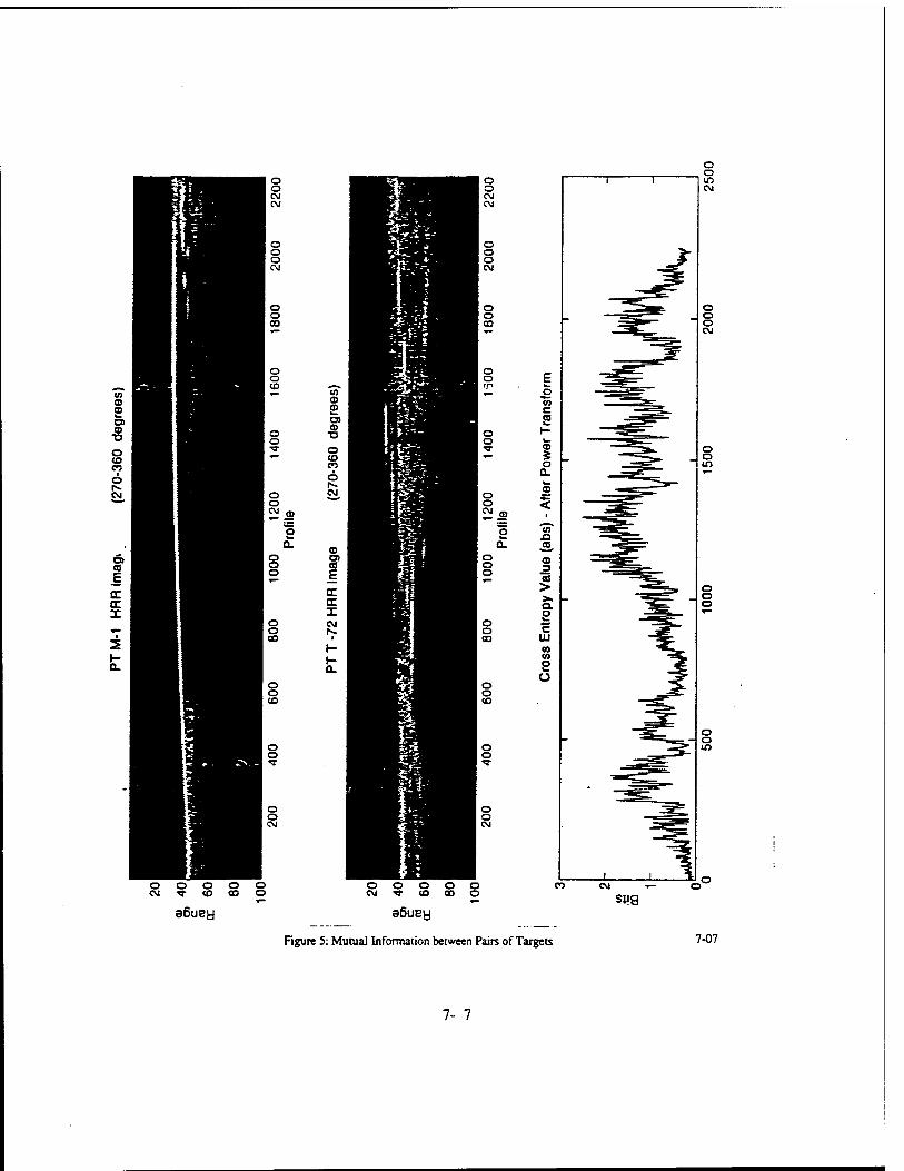
o o <N eg

I o CVJ

CO

o F f.O w. ,— o

m c C3

o H o w ^- CB

* O a. w C9 o «: o <

o w £} a. CS o o o

cs 3 es > >s Q. O

o o c CO III

01 01 o O o

o (O

o , o CM

a6uBu a6uey

Figure 5: Mutual Information between Pairs of Targets

sug

7-07

7- 7

• Task 2: We compared the informational entropy of range profiles, the same quantity as described above, for all targets before and after applying the power transform. Figure-4 shows the plots for the entropy values in the two cases.

- It is evident from these plots that throughout the target's 360 degrees the entropy value increases by an almost constant amount as a result of applying the power transform. However, the relative amount of information in various regions of a target remains the same.

• Task 3: Computed Mutual information for all pairs of targets. This study compared regions of targets and showed which regions were similar/different to each other from the perspective of informational entropy. A sample output is shown in Figure-5.

5 Seeking Good Features

Based on the insight provided by the above studies we designed a set of hierarchical features to be extracted for the HRR Data set of each target. An overview of these features can be summarized by the three-level binary tree shown in the following diagram.

2

<> 4 5

3 <v 6 7

One such binary tree corresponds to one range-profile signal similar to the one shown in Figure- 1. Each such signal is 100-points wide, we examine all 10-point wide regions and determine the region with maximum amount "Energy" in it. An estimated measure of energy is obtained by the product of informational entropy in the 10-point wide region and the average value of the signal in the region. The center cf this 10 point wide region is called the location of the corresponding energy amount.

For a signal we determine the location of the maximum energy and assign it to the node number 1 of the binary tree. The signal is then partitioned at this point into two parts. The Left Part contains the signal that lies to the left of the 10-point region of maximum energy and the Right Part contains the signal that lies to the right of the maximum energy region. Determination of regions of maximum energy and partitioning is recursively continued until the seven nodes of the above tree have been filled. It is possible that many nodes of this tree may remain unfilled due to the nature of a particular signal.

7-v8

This system was fine-tuned and binary trees determined for the 180 2-degree templates of each target. That is, data for each target was reduced to 180 template signals by summing over 2-degree regions and then a binary tree was generated for each resulting template signal. Figure-6 shows a plot of these binary trees for a target. This plot only shows the locations where regions of high energy are found in the consecutive template signals. Solid line shows the locus of the location stored at node number 1 of the tree. Loci for the locations stored at node numbers 2 and 3 of the tree are shown by dashed line; and those for node numbers 4 and 7 by the dotted lines. The plot shown in Figure-6 presents a very good presentation of the main scatter centers for the target. This is a validation of the fact that the features capture good physical properties of the target from the HRR data. There is much noise, however, in the plot in Figure-6 and the definitions of features need to be further refined before a recognition system is finally constructed.

The binary tree representation stores at its nodes information about the locations and amounts of energy at the various energy-centers of a signal. This information can be used to synthesize new attributes at each node. For example, a moment-of-energy can be computed at each node based upon the moments-of-energy at the children nodes. A number of encouraging results were obtained in this direction but they also pointed towards an anomaly having its origins in the data-reduction stage.

5.1 A Problem with Template-Making

Each range-profile is a signal consisting of 100 values. In our HRR dataset a signal is obtained after every 0.04 degree movement around a target, and from a fixed elevation. This results in 9000 range-profiles being collected for a target, for an elevation. Templates are made by Averaging contiguous sets of 50 profiles each, assuming that the shapes of signals change only gradually.

The assumption that the shapes of signals change only gradually is largely true but there are numerous points where the transitions in signals' characteristics are sharper than the usual. When the sharper transitions are included within a templates and the signals averaged, the resulting templates have larger variation from the individual signals contained in the template. More formally, let us define ith range-profile as Pi(k) where k takes the values from 1 to 100. The mth

template tm is formed by averaging 50 contiguous range profiles as follows:

m*50

tm(k)= £ Pi(k) for k = 1....100. (2) f=(m-l)*50+l

. The av?r.~f;?J template signals-differs from each of the 50 individual signal? of which it is an avsr.ajrc. One way to define this error for the Vth range profile is by deferrohurig the Square-Error as follows:

Ei{k) = {abs{Pi{k) - tm{k)))2 for k = 1....100. (3)

The average of the Square-Error vector for a template can be computed as follows:

m*50

MSEm{k) = Y, Ei(k) for k = 1....100. (4) i=(m-l)*50+l

Figure-7 shows a template signal and its corresponding MSE signal. A measure of how much, on the average, a template varies from its constituent signals can be obtained by computing the area

7--9

(A

s Q. E a> a> CD

a> ■o

a> S

a

01

o o

Figure 6: A Plot of Binary Tree-structured Attribute Values 7-10

7-10

under the MSE curve shown in Figure-7. This area can be computed as:

100

ERRORm = Y, MSEm{l). (5) /=i

5.2 Uniform-Width Templates

The prevalent method for making templates is to partition the entire angular region around a target into equal-sized angular regions and then average the range-profiles falling within the region of each template. For our dataset, if we want to make 2-degree templates then contiguous sets of 50 profiles would be taken to form template signals. The starting points of these templates would be at profile numbers: 1, 51, 101, 151 ...8951. The average error resulting from forming 180 uniform-width templates in this way can be determined as:

180

Avg-MSE = l/lS0{Y,ERRORm- (6)

5.3 Variable-Width Templates

Our insights into the HRR data for target vehicles suggested that the ERROR resulting from averaging within a fixed-width template is high because signatures of significantly different characteristics get averaged together. That is, the angular regions around a target where the transition in signal shapes is sharper than the average gradual rate of change, the resulting template signals have higher value for ERROR. The ERROR-value can be decreased if the boundaries of the 180 templates are moved around and readjusted in such a way that the points of sharper transitions form the boundaries between templates. The problem now is to determine the placements for the boundaries such that the ERROR is minimized.

5.4 Heuristic Search for Template Boundaries

The problem of finding the template boundaries so as to minimize the value of ERROR is an optimization problem and can possibly be formulated in a number of different ways. After our initial attempts at formulating it in terms of some relaxation algorithms did not show much promise, we formulated it as a heuristic search problem. Main steps of this algorithm are as follows:

• 1. TaVe --. Wr.-.dow -".-f 5-degree width and slide it. by changing one range profile at a time, across the entire dataset for the target. Determine the value of MSE for each 5-degree template as the window slides across the target. Figure-8 shows a plot of the MSE value for one target.

2. Rearrange the points according to increasing values of their corresponding MSE values.

3. Select a subset of 50 template-starting points from the above list such that:

(a) Every range profile gets included in one or the other template. (By a template we refer to all those contiguous range profiles that will be averaged to obtain a representative template signal.)

7-11

100

Figure7: A Template Signal and corresponding MSE signal

1000 2000 3000 4000 5000 6000 7000 8000 9000

Figure 8: Mean Square Error for a sliding window of 2-degree width (Fire Truck)

7-12

(b) No two templates overlap.

(c) Starting points are chosen as much as possible towards the beginning of the list created in step-2.

A set of points generated as above constitutes one hypothesis about the template starting points. It is possible to generate a number of such hypotheses. After generating these hypotheses we have to find the best solution by suitable refining the most promising hypotheses by operators that change the staring point? of templates. This is achieved by the following step that performs a heuristic search.

4. Run a heuristic algorithm (modeled after A* search algorithm) with the following search operators:

(a) Expand a template to include more range profiles.

(b) Partition a template into two templates in such a way that their weighted MSE is minimized. The weightings are provided by the width of each partition.

(c) Merge two adjoining templates into one.

At each step of this algorithm a heuristic function is used to determine the hypothesis that should be selected for modification by one of the above steps.

5. The algorithm terminates when the number of templates has reached 180.

For the case of uniform-width templates the value AYg-MSE as defined above gives an indication of "Goodness" of the templates. The same function can be employed to determine the similar "Goodness" for the variable-width templates generated by our search algorithm. However, there is one difference that we must account for. When the templates are of different widths their contribution to the average error for all the templates should be in proportion to their individual widths. That is.

180

Avg - MSE = {l/9000){^2{ERRORrr. * Widthm) where (7) n=l

Widthm is the width of the mth template. The heuristic functions chosen by us for the above described search algorithm were designed to minimize this error function. It is also possible to alter these heuristic functions and minimize some other measure of error, such as,

Avg -MSE=(Max™l(ERROPm*Widthm). (8)

5.5 Results of Search Algorithm

We plotted the values of Avg-MSE for an equal number of uniform-width and variable-width templates constructed from the same regions of all targets. The plot for the fire-truck target is shown in Figure-9. It can be seen from this plot that for the case of 180 templates the average value of error for variable-width templates is about 12% less than the error for the same number of uniform-width templates. Or alternatively, about 30% fewer templates of variable-width need to be constructed for maintaining the same error rate. Figure-10 shows the distribution of error- values for individual templates for the two types of template construction procedures.

7-13

FTR: Comparison of MSE for equal and variable sized templates (0-360 degrees)

50 100 150 Number of Templates in 360 degree region

200

Figure-9: Mean Square Error for Equal Number of Uniform and Variable Width Templates

7-14

Dianbution of MSE-vaM tor 120 Uriterm »mplatu

20 25 30 MSETtmplatt-Siz«

FTR Distrfcutjon o( MSE viiiw «or 120 vmrabnl« sind umpuias (0-120 d*grw)

20 25 30 MSE («rut' l*mobt*-anOm

Figure 10: Distribution of Error among Uniform and Variable Width Templates

7-15

This result is significant in that is demonstrates that by adjusting the boundaries of templates it is possible to significantly reduce the Mean-Square Error within each template. This should result in enhanced performance for those implementations of ATR algorithms that use variable- width templates instead of uniform-width templates.

The comparison between uniform-width and variable-width templates was performed for each of the five targets. It is evident from these tests that the weighted average of the MSEs can be reduced by approximately 10-15 percent, or alternatively, the same MSE level can be maintained by constructing 30-40 percent fewer variable-width templates.

The above results have been possible with the help of a very crude heuristic implemented only for demonstrating the correctness of the approach. The intuitive explanation for the improvement is that the structural features of the target vehicles are aligned at the boundaries of variable-width templates. It is possible to improve these heuristics and obtain better reduction in the MSE values by constructing variable-width templates.

6 Conclusion

The main contribution of this research has been the demonstration of an algorithm for efficiently constructing variable-width templates. These variable-width templates result in template signals for ATR that have significantly smaller data-compression error. This can help increase the performance of ATR systems. The scope of this study was limited and the actual ATR tests could not be carried out to ascertain the extent to which the performance of ATR can be improved.

Other contributions of this study are the insights that have been obtained into the characteristics of the HRR data for ground vehicles.

7-J6

ROBOT PATH PLANNING

into

CAVITIES DEFINED BY SPLINES

Alley C. Butler, Ph.D., P.E. Associate Professor

Mechanical & Industrial Engineering Dept.

Louisiana Tech University P.O. Box 10348

Ruston, LA 71272-0046


U. S. Air Force Materials Direcotrate (WL/MLIM) Wright Patterson AFB


Boiling AFB, Washington, DC.

and

Air Force Materials Directorate

October 1996

8-1

Alley C. Butler Robot Path Planning into Cavities defined by Splines

ABSTRACT

This report describes the development of a robot path planning system in which computational geometry is

used to generate an optimal robot path. The architecture of this system makes extensive use of B-splines. The

system is designed to support non-destructive testing of jet engine parts which contain multiple cavities. These

cavities are modeled by B-splines, and a Voronoi tree is developed by finding the intersection points for offset

curves or hodographs from the B-splines. In a manner similar to the Voronoi diagram, the Voronoi tree is

maximally distant from adjacent obstacles. This Voronoi tree, therefore, represents the path with greatest

clearance. For this reason, the Voronoi tree is used to guide path development for a single robot manipulator

which is inserted into the cavities. The addition of potential field methods allow development of complete path

information for the robot manipulator, based on attaching the potential field to the robot arm. In this report, a

literature survey is provided, and the techniques for finding a Voronoi tree are described. Next, the adaptation of

these techniques to develop manipulator paths using a potential field is discussed. Further evolution of the

methodology is outlined, and conclusions with recommendations are provided.

8-2

TABLE OF CONTENTS

Abstract 8-2

Table of Contents 8-3

Introduction 8-4

Literature Survey 8-5

Development of a Spline Based Model Finding the Voronoi Tree 8-9 Adding Linkages 8-10

Evolution of the Methodology 8-12

Conclusions and Recommendations 8-13

Acknowledgment 8-14

References 8-14

8-3

INTRODUCTION

Reliability of high performance jet aircraft engines is important to the combat survival of the pilot and the

aircraft. This reliability is ensured by periodic non-destructive inspection of the jet engines. For the Pratt and

Whitney F100-PW-229 engine, the inspection is done on a partly automated basis. Further automation of non-

destructive inspection has the potential for dramatically reducing engine inspection costs, thereby allowing the Air

Force to improve affordability. Figure 1 shows a cut-away view of the F100-PW-229 jet engine (Pratt & Whitney,

1996).

Figure 1 - Cutaway View of F100-PW-229 Engine (Pratt & Whitney, 1996)

Present methods involve eddy current inspection of engine parts using a Cartesian robot system. The path

planning process for these Cartesian systems takes approximately 25 hours of work for manual path planning

through conventional teach pennant technology. Recent advances in the development of algorithms for automated

robot path planning have reduced this tedious and manpower intensive process, significantly to a matter of

minutes. However, the present techniques are not optimal in nature, and the occurrence of undetected collisions

requires additional computational steps.

One of the more challenging inspection processes, involves inspection of engine internals which form a set

of cavities, presently inspected by a Cartesian robot with a probe for flaw detection using eddy currents. These

cavities must be entered by a robot manipulator without collision with the part that is being inspected. This

involves developing a path which describes the motion of the robotic arm as it moves the probe into position for

inspection. The beginning point is called the home position by those involved in operating the robot, but the

terminology in the literature typically discusses movement from a start position, S, to a goal position, G. Figure 2

shows a sectional view of this process for the eddy current inspection of engine internals.

8-4

The sectional view represents a three dimensional engine part in two dimensions. This is appropriate, since

the engine is symmetric about its central axis. For the purpose of path planning, two dimensional analysis can be

undertaken as a simplification of the more complex three dimensional problem, because of symmetry about the

central axis. This approach, in which the path plan is developed in two dimensions and subsequently checked in

three dimensions, is the currently used method. It is also the approach employed in this study.

S or Home

Figure 2 - Sectional View for Robot Path Planning

The presently employed path planning method includes a number of steps which provide a path without

collision from S to G (Chemaly, 1996). The planning process begins with the development of a straight line from

S to G. If this does not intersect a boundary, then no adjustments must be made. However, this is unlikely.

Adjustments are made for those parts of the line between S and G which interfere (intersect) with the engine part.

The adjustments are developed by replacing the portions of the straight line path which interfere, with a path

which follows the surface of the engine part. This is distinctly similar to the method used by Lumelsky's (1991)

Bug-2 algorithm. Once collisions are eliminated by replacing intersecting paths with paths following the part's

boundary, a limited technique for improving the path can be employed. This limited technique finds shorter paths

by finding straight line motions which eliminate segments of the path. The result from this sequence of steps is a

path which is similar in principle to the visibility methods described by Lozano-Perez and Taylor (1989), and

identical to the "string tightened path" discussed by DuPont and Derby (1988).

In the visibility methods, the path is very close to collision, similar to a string which is stretched tight

against all obstacles. This is done to shorten the distance traveled. Unfortunately, this similarity to visibility

techniques has important drawbacks in the present application. Because the present technique shortens the path in

a manner identical to the visibility methods, the path is close to collision for some portions of the planned path.

8-5

3D """ "*" * «—«. -*. a«ional tae Mt, computationa]

deserve. Tie Voronoi Tee is general through ^ nse of nff , ' "*"*' ,he "^ V™» - 's

»*■ the engine pan,. „ shouId „ noM „^ * * ~ «*« ""» « ■»*«*. » <b. B-spUnes which

r*to-—^-t^sr-■;—-— described in this study. (W17MLIM) and subsequent application as

-isions. The optima, p.. deveI ^' £ * "" ^ « ** - "* distant from „ p0Bmia,

fro, a,, holies as * Senses ta /To U 7 " "" "" "*" ™ '° h ""^ —'

—« which is ho* convenient and „^JJ ^.T " "" ^ "^ *"*"' " «"» collision when «he p„h is converted to 3D I thJ "^ " *° ^^ *» F-** *»

discussion of the development of the Voronni , „ Y SphneS" ™s inclu^s a

—^.ichisjir;:::::^r^rr.-r——— ^e made. described, and conclusions with recommendations

LITERATURE SURVEY

- ^Z^rjTT^r moüo° ptani"g' sch™z - -* - -* , . ^ -1 °Ptima! motion p annins 21 pvnin™,„ .

8-6

the robot's environment, and typically, fc „„,y movi obJKt

optimal motion p,an„ine is reoa.YM **" For Ih» P«*l»> considered here,

êdranr:: ^^T^^"^^""*"»'-»«-

A,m„nghsoovai„e„986)coniide;soj :::: r»r;,r M a ^ "ave,ing teTO

B-splines to mode, obstades in «he form of cavities "" " "™ * ^ "*to ** -

Surveys of robot motion planning exi<:f wh;^h î„ •*. ,.

Hwang and Ahuja (1992) prov de aêx ^ "^ ^"^ ^ ^ '^> an K SIVC taX°n0my 0f the mo«on Planning process Th, r , approaches as cell decomposition, skeleton potential field .„H ♦„ * * CUITent

methods including visibility graph Voronoi d "' ^«^ ** *e skeleton nl„ . . "•'y^Ph.VoronQ.djagram, silhouette, and subgoal network Yann9S7^r planning m terms of physical snace <™™, *, network. Yap (1987) defines motion

—- - -i jr r;;:;7 ™:dr:::vrK'—-* - Planning and computational geometrv is d™ c S C°nneCti°n bctWBen motio"

-* * - .o .e use J Z^^ ^l t^ T ^ " ^ " ^ (Lee & Preparata, 1984; Böhm et al. 1984). P ^^ Md rela£ed science*

- a rrrr r^rcrrrme,hods invoive—* -— -er approach, he discusses «-JT^^jTCt " ^ "" "" *~ '" h-actable. In the configuration space all obstael m°ÜOn P,a"ni"g JJr*,em ™»

- .0 - reduced I a J^ZZ' ~ ~~ —■

configuration space (Langier, ,988,. Brooks (,983 sea T^ ^ 'nV°',eS ""* """^

confignration space, as regions of o,eLuT , W ""^ " ^ '" «■*» ■»

eells (Brooks & Loamo-Perez 1985) In a re, , d " '°""" m0tion ™°"S *«

âceney rCafionships (SharfiTl^ ^XTl T* ™ " *""~ *» «* ~

«** Paths, deve,ops the graph from tTeTof ZT ^ **" "* ""* "

--^^*,-,^fÄzzzz:^zr~*^,"*h a search for a solution. manageable representation, and there is

*K Process of changing the problem representation to a..ow an efficient search fo , ■ • potential field methods as well. Hwang (1992^ de„ -K „■ U Ut,°n 1S preSent in

electrostatic potential assigned to ea h ol C " " "^ " **""* *"*» ** » «" obstacle. Based on tests of his system, Hwang states that his method is fast

8-7

and reaches solutions on all but a small «.t r>f „™M • , .

d,ss,pa.,ve terms ,o cause the snake ,„ find a goa, taion g* ^ «"» »"

witnpoysica, analogs ,Ppe„s ,„ ta com™ with^ ^ J£~* '»* ^ « °f ™« —

By seeking a position of lowest potential, an optimization process occurs On,!™, *,

m nummal „me (Wapenhans et al., 1994; Bessonne, 4 Ullemand mv TV ■ P

P—„g for some systems (Sandgre„ & Venkataram " 9 ^&t8I ^ 2 ^^

r::r °;r^to — -**-——". £ —i Venkataraman, 1989) and recursive quadratic programming (Leu & Singh 1988) A« ■ , ,

present application, cavities have been the obstacle Th«. cavities were recognized as natural candidates for the use of splines The use of NURBS , f splines) has become the predominant spline format NURBS „ (non-uniform, rational b-

by Piegl and Tiller (1987) Piegl (,99l as Ü " * *""" ^ ^ (1983)' «* ^ *<s /;. negl (1991) has provided a survey of NURBS properties.

-e,o ment of an":0::::zns r n"ded-Mer ™rk °n in~ °f **-—- *. 1989 Dokken 1985, !dT HO' "*'"" ^^ * "« » *" ,"~*» ^ «

cementation of splines (Bar„„i„ e, a .^l, ^ TT^ "^ ' ' ^ "" 1988) inw, ♦• ,, ' ; SederberS& Meyers, 1988; Kaufmann & Klass 1988). Intersections of lines and splines have been studied by Pantelic and Janevski (1989) Of co 7

--^^M^««^«,,^^..^«,—-—^-—o—o. ^«. «^o.«... --«^^r^ 'm this

A number of researchers have focused on offset curves or hodographs Klass nwnH , „

offset curves which follows the Hermite form (Foley et a, 1990) AH ^(IW)dB^''^*r by Pham (1988) Till. A „ ^ ^ Unif0™ B"sPlines was studied vy rnam (tyss). Tiller and Hansen (1984) and Coauillart naxn « t- ^ NURBS oth u , ^oquillart (1987) worked on the development of offsets for

- - .lines is a corop.e, process, an. ,ey taher a. ^ ^ZZ ^^^

(Tiller & Hansen, 1984). Despite the complexity, detecting intersections with offset curves is a key process in

computational geometry, for path planning using splines.

In addition to path planning using splines, the use of spline architectures is useful in another way. The path

planning process outlined here develops an ordered sequence of points in 2D for the robot and its joints to traverse.

This ordered sequence must be translated into a continuous path with smooth and continuous motion. This means

that the C , C , and C2 properties of B-splines can be used to avoid abrupt changes in velocity and acceleration.

Development of splines from a sequence of points has been studied by Papamichael and Soares (1987) and by

others. The use of these splines for the control of robot manipulators has also been demonstrated (Patel & Lin,

1988; and others). From these this prior work, it is apparent that development of robot path plans using splines is

easily feasible.

DEVELOPMENT OF A SPLINE BASED MODEL

Finding the Voronoi Tree The name Voronoi tree has been chosen to describe the technique outlined here, because of the similarity to

the Voronoi diagram which is maximally distant from all objects in a two dimensional space (Lozano-Perez &

Taylor, 1989). Both the Voronoi diagram and the Voronoi tree described here, provide paths for robot motion

which avoid collisions to the greatest extent allowed by the geometry, and this should permit solution of the path

planning problem in two dimensions without difficulties when the plan is checked in 3D.

The cavities found in the jet engine part, as shown in Figure 2, represent parts which should be described by

splines in a CAD system. The Voronoi tree is developed directly from the spline geometry. Therefore, this spline

based approach is both natural and efficient for path planning.

Offset curves from splines can be found for the cavity geometry. The utility of these curves or hodographs

was originally recognized by Air Force personnel (Dr. LeClair) with subsequent application here. These offset

curves or hodographs follow the contour of the spline, but they exist at an offset distance, d, from the spline. The

equations which describe the offset curves are parametric in t in a manner similar to the spline curves (Hoschek,

1985):

x'(t) = x(t) + d(nx) (1)

y'(t) = y(t) ± d(ny) (2)

where x\ y' describe the offset curve, x, y describes the spline, d is the offset distance, and n represents the

normal to the spline curve. Offset curves can be developed for different values of d.

8-9

f offse, curves fron, ,»„ surfaces described by splines intersec., dae p„in, of in.ersec.ion is a distance d ton,

«* spl,ne curve. So, .be poinK of in.erscc.ion for effse. curves (having idendca, values of d) are e,uidis.an. Iron,

^ sur.es. B, „erseebng m„,.ip,e * curves widn differen, valuea of d, poi„.s wfdch are e,ua„yIs I

Adding Robot Linkage

Altogb the Voronoi tree represems a path „hidl „ e^ally dis.a„. <o ail bounding sP,i„es i. does „o. prov.de ,„form,ion „ how . robo., ,inkages shou,d „ control]ed _ _ , cavjty fc ^ _ j^ '

»P,a,,„ , required .0 find the robofs „ptinra, coupon as i. inverses the Vorouoi tree fron. S , OT

»-*-, th.s portion of.be pa,b p.anning probieu,, offse. curves are again retired. These offset curv« I

»n ^.opro.dea.easnreof.bepo.en.ia, for intersection. Assuch, doe approacb ,8 sindiar .0 po,e„d I

: z rr. rprincipie *** ^ ^™ -*- - * - *— -- «£- fie,d „h.ch ,s used ,0 surround ai, obs.aeies. A,.bougb dais ardficia, po.en.ia, Md is based on stap„

add,g ™ .0 doe pa* pianning „goridon, the, added ,ems provide a means of ^iUng- ,be robo, a™

im- optimai mM s°'a ■—- - - * -*- - ~:

Offset Curve from Spline

Figure 3 - Developing Poi„,s „„ the Voronoi Tree with Inlersecdng Offse. Curves

In .he .echnique advocated here, .here is one difference ,0 o,ber po,e„,ia, deld me,b*. Most po.en.ia,

«elds are ass„c,a,ed wifb obs.acles. However, if ,ha. approach is used here .here w.,1 ta n,u„ip,e offse, £2

8-10

the offset curves will require significant computational time. Additionally, the intersections between the offset

curves and the polygonal boundaries of the robot must be found. This is a relatively complex computational task.

To limit these difficulties, an equivalent approach is used. The potential field is attached to the robot arm.

This allows offsets to be constructed as simple lines which are parallel to the polygon which represents the robot's

arm. These lines are intersected-with the splines which form the cavity. This represents a very efficient way to

represent and compute potential, since the lines all intersect with a spline which has known control points. (The

control points of the offset curve would have to be determined as added computational burden.) These control

points form a convex hull around portions of the curve, and this permits checking of line intersections with the

convex hull. The checking of intersection with the convex hull is a local property of the spline curve, and line-

spline intersections can, therefore, be rapidly and easily found. This is a significant innovation directly inspierd by

close collaboration with an Air Force research enginer (again, Dr. LeClair).

As presently implemented in C language code, the intersection of a line and spline is found by a hierarchical

method which rapidly excludes trivial cases in the computational hierarchy. This process of descending down the

hierarchy is developed to maximize computational speed. It involves excluding line spline intersection first by a

bounding box. Then, exclusion of line-spline intersection is accomplished by checking for intersection with the

convex hull for the spline. If the convex hull is intersected, then Newton-Raphson procedures are employed to

determine the point of intersection (Mortonson, 1985; Mortonson, 1990) using data from the earlier computations

on the convex hull. This provides line-spline intersection data rapidly and avoids expensive computation for non- intersecting cases.

Once line-spline intersections are determined, the level of potential field interference with the cavity

boundaries as obstacles can be determined. This potential field is based on the length of the offset lines which

intersect the splines. Equation (3) below shows how the potential function should be constructed. The first term

involves the development of a measure for the Euclidean distance between the manipulator tip at xt, y, and a point

on the Voronoi tree as x*, y*. This term is multiplied by a factor K which is adjusted to obtain a good balance

between robot arm position and motion of the manipulator tip relative to the Voronoi tree. The second term sums

the product of the weight associated with an offset curve as ws and the length of intersection as L, between the

offset curve and the spline describing the cavity. The value of Ls should reflect the severity of interference between

the obstacle and the offset line. Of course, offset lines at greater distance from the robot arm would have lesser

weight as Wi, since the probability of collision is less. The result is a measure as * of how close the robot arm is to

a collision.

*(**) = W(x*-xt)2 + (y*-yt)

2 + £ Li w. (3)

8-11

With this measure available, an optimal position for the robot arm can be found to avoid collision. This

technique is illustrated in Figure 4 for three linkages and a portion of the part.

Spline for Part Boundary

Robot Arm

Offset Curve (Line)

Figure 4 - Developing a Potential Field Attached to the Robot Arm

EVOLUTION OF THE METHODOLOGY

Time allocated to the research has been finite, and choices regarding which veins of research to pursue

aggressively had to be made. Despite limitations in time and resources, several key steps have been completed

which represent an important beginning. The steps which were completed include an orientation to the problem,

an in depth literature review (which is only partially represented in this report), development of key research

concepts and approaches, and commencement of programming for a prototype system. The programming was

conducted in the C language in a Unix and X Windows environment.

Due to limited time, some processes are deferred. These include the choice of offset curve architecture, and

the optimization of hodograph-hodograph intersection algorithms. Present methods require human computer

interaction which necessitates limited user involvement.

Additionally, programming is continuing on the development of the potential field technique. Code for

representation and rendering of splines as non-uniform, non-rational b-splines is presently in place. Intersection

algorithms for line-spline intersection have been developed using methods outlined by Prasad (1991) as improved

by Shafer and Fuestel (1992) for intersections with the convex hull. These methods are hierarchical and represent

an approach designed for fast computation. The development of other functions and routines for the path planning

system are continuing, with the development of algorithms to determine O in equation (3) as the next priority.

8-12

After development and testing of this code, a simulated annealing approach is planned for the optimization of $.

This will demonstrate the feasibility and utility of the overall Voronoi tree and potential field methods.

CONCLUSIONS AND RECOMMENDATIONS

As a result of this investigation, there are a number of conclusions which can be drawn from this work.

These conclusions are represent in the following:

1. Most of the literature discusses path planning in an environment with obstacles described by polytopes

(polygons in 2D and polyhedra in 3D). A few other papers discuss path planning using other regular

geometric shapes like the ellipse, circle, or cone. The author is unaware of any work which investigates path

planning into cavities defined by splines.

2. Computational speed is a key issue in the benchmarking of path planning systems. There is a trade-off

between using faster methods which require extensive checking and rework due to collisions in 3D, and a

method which may take longer to avoid the extensive checking and rework. Therefore, computational speed

continues to be an important item on the research agenda.

3. It is anticipated that solutions will be sensitive to the values of d in the offset curves or hodographs (equations

1 and 2), and to the values of K and w; in equation (3). Experience with the method should be the best guide

to generate proper solutions.

4. The algorithms described here for Robot path planning have no proof of convergence. The result is that the

algorithms may fail under certain conditions. It is expected that the outcome should, however, be similar to

Hwang's (1992) results in which failure occurs over a very limited subset of problems.

There is one key recommendation: The work which was begun through this study should continue. This

involves additional programming and program testing which can be accomplished in the coming months. As

secondary recommendations, robot dynamics/kinematics should be considered more fully in future approaches

(Seereeram & Wen, 1995; Xue & Sheu, 1989), and a migration to a continuous path approach should also be

considered (Brady, 1982).

The research outlined here uses a novel approach to accomplish path planning for robot arms which travel

into cavities. It is believe that the methods will prove superior to existing techniques, and improvements will drive

down inspection costs. This will make greater levels of reliability needed by the Air Force more affordable.

8-13

REFERENCES

Barnhill, R. E., G. Farin, M. Jordan, and B. R. Piper, 1987, "Surface/Surface Intersection," Computer-Aided Geometric Design, vol. 4, pp. 3-16.

Barnhill, Robert E., 1989, "Geometry Processing: Curvature Analysis and Surface-Surface Intersection," in Mathematical Methods in Computer Aided Geometric Design, (edited by) Tom Lyche and Larry L. Schumaker, Academic Press, Boston, pp. 51-60.

Bessonnet, G. and J. P. Lallemand, May 2-6, 1993, "Planning of Optimal Free Paths of Robotic Manipulators with Bounds on Dynamic Forces," Proceedings of the IEEE International Conference on Robotics and Automation Atlanta, GA, pp. 270-275.

Böhm, Wolfgang, Gerald Farin, and Jürgen Kahmann, 1984, "A Survey of Curve and Surface Methods in CAGD," Computer Aided Geometric Design, vol. 1, pp. 1-60.

Brady, Michael, 1982, "Trajectory Planning," as chapter 4 in Robot Motion: Planning and Control, (edited by) Michael Brady, John M. Hollerback, Timothy L. Johnson, Tomas Lozano-Perez, and Matthew T. Mason, The MIT Press, Cambridge, MA, pp. 221 -243.

Brooks, Rodney A., March/April 1983, "Solving the Find-Path Problem by Good Representation of Free Space," IEEE Transactions on Systems, Man, and Cybernetics, vol. SMC-13, no. 3, pp. 190-197.

Brooks, Rodney A. and Tomas Lozano-Perez, March/April 1985, "A Subdivision Algorithm in Configuration Space for Findpath with Rotation," IEEE Transactions on Systems, Man, and Cybewrnetics, vol SMC-15 no 2 pp. 224-233. ' ' '

Carriker, Wayne F., Pradeep K. Khosla, and Bruce H. Krogh, May 13-18, 1990, "The Use of Simulated Annealing to Solve the Mobile Manipulator Path Planning Problem," Proceedings of the 1990 IEEE International Conference on Robotics and Automation, Cincinnati, OH, pp. 204-209.

Chemaly, Adel, July 26, 1996, private communication with Alley Butler, Technosoft, Inc., Cincinatti, OH,

Coquillart, Sabine, July/August 1987, "Computing Offsets of B-Spline Curves," Computer Aided Design vol 19 no. 6, pp. 305-309. '

Dokken, Tor, 1985, "Finding Intersections of B-Spline Represented Geometries using Recursive Subdivision Techniques," Computer-Aided Geometric Design, vol. 2, pp. 189-195.

Dokken, Tor, Vibeke Skytt, and Anne-Marie Ytrehus, 1989, "Recursive Subdivision and Iteration in Intersections and Related Problems," in Mathematical Methods in Computer Aided Geometric Design, (edited by) Tom Lyche and Larry L. Schumaker, 207-214.

DuPont, Pierre E. and Stephen Derby, Oct. 16-22, 1988, "An Algorithm for CAD-Based Generation of Collision- Free Robot Paths," Proceedings of the NATO Advanced Research Workshop on Sensory Robotics for Limp Materials, Ciocco, Italy, pp. 433-465.

Farouki, R. T., 1985, "Exact Offset Procedures for Simple Solids," Computer Aided Geometric Design vol 2 DD 257-279. ■ ' rr-

Farouki, R. T., 1986, "The Approximation of Non-degenerate Offset Surfaces," Computer-Aided Geometric Design, vol. 3, pp. 15-43.

8-14

Farouki, R. T. and T. Sakkalis, September 1990, "Pythagorean Holographs," IBM Journal of Research and Development, vol. 34, no. 5, pp. 736-752.

Foley, James D., Andries van Dam, Steven K. Feiner, and John F. Hughes, 1990, Computer Graphics, Principles and Practice, Second Edition, Addison Wesley, Reading, MA, pp. 471-530.

Forrest, A. R., July 1980, "The Twisted Cubic Curve: A Computer-Aided Geometric Design Approach," Computer Aided Design, vol. 12, no. 4, pp. 165-172.

Gasmi, Bernadette, and Claude Reboulet, Oct. 16-22, 1988, "Trajectory Planning and Obstacle Avoidance," Proceedings of the NATO Advanced Research Workshop on Sensory Robotics for Limp Materials, Ciocco, Italy, pp. 244-261.

Hoschek, Josef, March 1985, "Offset Curves in the Plane," Computer Aided Design, vol. 17, no. 2, pp. 77-82.

Hoschek, Josef, 1988, "Spline Approximation of Offset Curves," Computer Aided Geometric Design, vol. 5, pp. 33-40.

Hwang, Yong K. and Narendra Ahuja, February 1992, "A Potential Field Approach to Path Planning," IEEE Transactions on Robotics and Automation, vol. 8, no. 1, pp. 23-32.

Klass, Reinhold, September 1983, "An Offset Spline Approximation for Plane Cubic Splines," Computer Aided Design, vol. 15, no. 5, pp. 297-299.

Kaufmann, E. and R. Klass, 1988, "Smoothing Surfaces using Reflection Lines for Families of Splines," Computer Aided Design, vol. 20, no. 6, pp. 312-316.

Koren, Yoram, April 9-11, 1991, "Potential Field Methods and Their Inherent Limitations for Robot Navigation," Proceedings of the 1991 IEEE International Conference on Robotics and Automation, Sacramento, CA, pp. 1398- 1404.

Laugier, Christian, Oct. 16-22, 1988, "Planning Robot Motions in the SHARP System," Proceedings of the NATO Advanced Research Workshop on Sensory Robotics for Limp Materials, Ciocco, Italy, pp. 151-187.

Lee, D. T. and Franco P. Preparata, December 1984, "Computational Geometry - A Survey," IEEE Transactions on Computers, vol. C-33, no. 12, pp. 1072-1101.

Leu, M. C. and S. K. Singh, July 4-6, 1988, "Optimal Planning of Trajectories for Robots," Proceedings of the NATO Advanced Research Workshop on CAD Based Programming for Sensory Robots, Ciocco, Italy, pp. 467-477.

Lozano-Perez, Tomas, and Michael A. Wesley, 1979, "An Algorithm for Planning Collision-Free Paths Among Polyhedral Obstacles," Communications of the ACM, vol. 22, no. 10, pp. 560-570.

Lozano-Perez, Tomas, 1982, "Task Planning," as chapter 6 in Robot Motion: Planning and Control, edited by Michael Brady, John M. Hollerback, Timothy Johnson, Tomas Lozano-Perez, and Matthew T. Mason, MIT Press, Cambridge, MA, pp. 485-585.

Lozano-Perez, Tomas, February 1983, "Spatial Planning: A Configuration Space Approach," IEEE Transactions on Computers, vol. C-32, on. 2, as reprinted in Autonomous Mobile Robots: Perception, Mapping, and Navigation, edited by S. S. Iyengar and Alberto Elfes, pp.395-407.

Lozano-Perez, Tomas and Russell H. Taylor, 1989, "Geometric Issues in Planning Robot Tasks," as Chapter 6 in, Robotics Science, edited by Michael Brady, MIT Press, Cambridge, MA, pp. 227-261.

8-15

Lumelsky VI., 1991 "A Comparative Study on the Path Length Performance of Maze-Searching and Robot Motion Planning Algorithms," IEEE Transactions on Robotics and Automation, vol. 7, no. 1, pp. 57-66

McLean Alistair and Stephen Cameron, May 2-6, 1993, "Snake-Based Path Planning for Redundant Manipulators, Proceedings of the 1EEE International Conference on Robotics and Automation, Atlanta, GA, pp

SS) lit J" B" ^mbCr IT' "An A1S°rithmic APProach to Some Problems in Terrain Navigation," Artificial Intelligence, vol. 37, no. 1-3, pp. 171-201.

S^JTHSSI w-SS:Computer Graphics Handb00k'Geometry and Mathematics>industriai p*». New Mortenson, Michael E., 1985, Geometric Modeling, John Wiley and Sons, New York.

Papamichael, N. and M J. Soares, 1987, "Cubic and Quintic Spline-on-Spline Interpolation," Journal of Computational and Applied Mathematics, vol. 20, pp. 359-366. 7

Patel, R. V. and Z. Lin, August 8-12, 1988, "Collision Free Trajectory Planning for Robot Maninulators "

Pantelic, Dejan V. and Zoran D. Janevski, 1989, "A New Kind of Splines and Their Use for Fast Ray-Tracing in Reflective Cavities, Computer Physics Communications, vol. 55, pp. 5-11.

Papamichael, N. and M. J. Soares, 1987, "Cubic and Quintic Spline-on-Spline Interpolation," Journal of Computational and Applied Mathematics, vol. 20, pp. 359-366. Journal of

Pham, B., 1988, "Offset Approximations of Uniform B-Splines," Computer Aided Design, vol. 20, no. 8, pp. 471-

Piegl, Les and Tiller, Wayne November 1987, "Curve and Surface Constructions using Rational b-Splines" Computer-Aided Design, vol. 19, no. 9, pp. 485-493. w-opimes,

Piegl, Les A, 1991, "Rational B-Spline Curves and Surfaces for CAD and Graphics," in State of the Art in

^^cSîp S^f" andMOddin8< (£dited by) DaVid R R°^s and Rae A Earnshaw, Springer-

Son, ^V'û'r"11011 of Line Sesments'"Gmphics Gems"'edited by james Mv°>Academic *«• wf fmîT U^lTechnol°Sies CorP-> 1996- "F100-PW-229 Increased Performance Engine" brochure 1991-10M, PO Box 109600, W. Palm Beach, FL 33410-9600'. orocnure

Rohnert, Hans, 1991, "MovingaDisc Between Polygons," AZ^nrWa, vol. 6, pp. 182-191.

ReafS An""0 \ yepnkataraman' ?f 17'21' 1989' "Robot Path PlanninS ™ Simulated Annealing: A Near

Real Time Approach, Proceedings of the ASME Design Automation Conference, pp. 345-351.

lt7T,u' J»7vand,^ ,Shadr' DeCember 1988' "A SUrvey of Motion Planni"g and Related Geometric Algorithms," Artificial Intelligence, vol. 37, no. 1-3, pp. 157-169. ueometnc

8-16

Sederberg, Thomas W. and Scott R. Parry, 1986, "Comparison of Three Curve Intersection Algorithms," Computer Aided Design, vol. 18, no. 1, pp. 58-63.

Sederberg, Thomas W. and Xuguang Wang, 1987, "Rational Hodographs," Computer Aided Geometric Design, vol. 4, pp. 33-335.

Sederberg, Thomas W. and Ray J. Meyers, 1988, "Loop Detection in Surface Patch Intersections," Computer Aided Geometric Design, vol. 5, pp. 161-171.

Seereeram, Sanjeev and John T. Wen, February 1995, "A Global Approach to Path Planning for Redundant Manipulators," IEEE Transactions on Robotics and Automation, vol. ll.no. l,pp. 152-160.

Shafer, Clifford A. and Charles D. Feustel, 1992, "Exact Computation of 2-D Intersections," Graphics Gems III, edited by David Kirk, Academic Press, Boston, pp. 188-192 & 491-495.

Sharir, Micha, and Elka Ariel-Sheffi, July 1984, "On the Piano Mover's Problem: Various Decomposable Two Dimensional Motion-Planning Problems," Communications on Pure and Applied Mathematics, vol. 37, no. 4, pp. 479-493.

Souvaine, D. L., 1986, Computational Geometry in a Curved World, Ph.D. Dissertation, Department of Computer Science, Princeton University, Princeton, NJ.

Tiller, Wayne, September 1983, "Rational B-splines for Curve and Surface Representation," IEEE Computer Graphics and Applications, vol. 3, no. 6, pp. 61-69. Discusses NURBS and they are needed.

Tiller, Wayne and Eric G. Hanson, 1984, "Offsets of Two Dimensional Profiles," IEEE Computer Graphics and Applications, vol. 4, no. 9, pp. 36-46.

Wapenhans, H., J. Holzl, J. Steinle, and F. Pfeiffer, 1994, "Optimal Trajectory Planning with Application to Industrial Robots," International Journal of Advanced Manufacturing Technology, vol. 9, pp. 49-55.

Whitsides, S. H., 1985, "Computational Geometry and Motion Planning," in Computational Geometry, (edited by) Godfried T. Toussaint, North-Holland, New York, pp. 311 All.

Xue, Quing and P. C-Y. Sheu, 1989, "Path Planning for Two Cooperating Robot Manipulators," IEEE Proceedings, pp. 649-657.

Yap, Chee-Keng, 1987, "Algorithmic Motion Planning," as chapter 3 in, Algorithmic and Geometric Aspects of Robotics, Volume 1, (edited by) Jacob T. Schwartz and Chee-Keng Yap, Lawrence Erlbaum Associates, Hillsdale, NJ., pp. 95-141.

Hwang, Yong K., and Narendra Ahuja, September 1992, "Gross Motion Planning - A Survey," ACM Computing Surveys, vol. 24, no. 3, pp. 219-291.

8-17

Importance of Current Crowding and Self-heating

Effects in a CdS/LaS Cold Cathode

M.Cahay

Associate Professor

Department of Electrical Engineering

University of Cincinnati

832 Rhodes Hall

Cincinnati, Ohio 45221

Final Report for:

Summer Faculty Research Program

Wright Laboratory

Sponsored by:

Air Force Office Of Scientific Research


and

Wright laboratory

November 1996

9-1

Modeling and Design of New Cold Cathode Emitters

Using Wide Bandgap Semiconductors

M.Cahay

Associate Professor

Department of Electrical Engineeering


ABSTRACT

We analyze the importance of current crowding in a new cold cathode emitter which consists

of a thin wide bandgap semiconductor material sandwiched between a metallic or heavily

doped semiconductor and a low work function semimetallic thin film. Potential material

candidates are suggested to achieve low-voltage (< 10 V), room-temperature cold cathode

operation with emission currents of several tens of A/ era2. We calculate the lateral potential

drop which occurs across the emission window of cold cathodes with circular geometry and

describe its effects on the emitted current density profile. The power dissipation in the

cold cathode is calculated as a function of a dimensionless parameter characterizing the

importance of current crowding. We determine the range of dc bias over which cold cathodes

of different radii must be operated to minimize current crowding and self-heating effects.

9-2

I. INTRODUCTION

Recently, there has been renewed interest into cold cathode emitters for applications to

a variety of electronic devices, including microwave vacuum transistors and tubes, pressure

sensors, thin panel displays, high temperature and radiation tolerant sensors, among others

[1, 2]. Introduction of such emitters would permit an unprecedented compactness and weight

reduction in device and equipment design. Low temperature operation in nonthermionic

electron emitters is very desirable for keeping the statistical energy distribution of emitted

electrons as narrow as possible, to minimize thermal drift of solid state device characteristics,

and to avoid accelerated thermal aging or destruction by internal mechanical stress and

fatigue. To keep the emitter temperature rise small appears easy if the emitters are built as

thin epitaxial films using vertical layering technology due to the extremely short heatpaths

and excellent heatsinking possibilities offered with this architecture. For an electron emitter

to be useful in microwave tube applications it should be capable of delivering current densities

in excess of 10 A/ cm2 and to sustain emission during operational lifetimes over periods of

105 hrs. To satisfy this requirement, the structural and chemical composition must be stable.

This rules out the historically practiced use of alkali metal films on emitter surfaces for the

lowering of electronic work functions. These films sublimate, evaporate or surface migrate

over time and end up on various surfaces inside the vacuum envelop.

Several cold cathode emitters have been proposed since their first successful demon-

stration by Williams and Simon [3] using a cesiated p-type GaP structure. A review and

criticism of the different cold cathode approaches was given recently by Akinwande et al.

[4]. In this work, we propose a new cold cathode emitter concept and use a simple model to

show that the new emitter is capable of achieving low voltage (< 10 V) room temperature

operation with emission current approaching 100 A/cm2 and large efficiencies. A prelimi-

nary report of this work has been published earlier [5]. The architecture of the structure is

shown in Fig. 1. The main elements in the design and functioning of such an emitter are

: (1) a wide bandgap semiconductor slab equipped on one side with a metallic contact [6]

or a heavily doped semiconductor (n++ — InP) on one side of an undoped CdS region that

supplies electrons at a sufficient rate into the conduction band and (2) on the opposite side,

a thin semimetallic film that facilitates the coherent transport (tunneling) of electrons from

the semiconductor conduction band into vacuum. Of importance is the mutual alignment

of the crystalline energy levels at the semiconductor-semimetal film junction. This requires

the use of new materials and development of their epitaxial growth technologies. For that

9-3

reason, the choice of InP as a substrate is particularly attractive since the lattice constant

of InP (5.S6 Ä) closely matches the lattice constant of the zincblende cubic CdS (5.83 Ä).

Furthermore, there have been recent reports on the deposition of crystalline layers of CdS on

InP by molecular beam epitaxy [7], chemical bath deposition [8], and pulsed laser deposition

[9]. The proposed cold cathode should therefore be realizable with present day technology.

As shown in Fig. 1(a), a thick metal grid is defined on the surface of the LaS thin

film to bias the structure. There are openings in the grid structure to expose the thin LaS

film which forms the active emission area of the cold cathode. Cathodes with rectangular

(Fig.l(b)) emission windows were studied previously [5]. Current crowding and self-heating

effects in cathodes with circular geometry (Fig.l(c)) emission windows will be considered

hereafter. The bias is applied between the back metallic contact and the metal grid with

emission occuring from the exposed LaS surface. If the applied voltage is equal or larger

than the semiconductor bandgap energy and the quotient of the applied voltage divided by

the semiconductor thickness approaches O.leV/A, then electrons are tunnel injected into the

conduction band and ascend during their travel across the semiconductor film to levels of

increasing energy. Referring to Fig. 2, the conduction band of the wide bandgap semicon-

ductor provides the launching site for electrons where they are - through a thin film - injected

into vacuum. This injection of electrons into vacuum becomes possible and is effective as

long as the semimetallic film is very thin and has a work function small enough so that its

vacuum edge is located energetically below the conduction band edge of the semiconductor.

This situation is referred to as negative electron affinity (NEA) for the semiconductor ma-

terial [10]. Depending on the particular materials choices, this implies that the semimetal

work function <J>M in relation to the semiconductor energy bandgap EG must obey one of the

inequalities 4>M < 0.5Ec or 4>M < Eg if an intrinsic or p-type doped wide bandgap semi-

conductor is used, respectively. A negative <f>M implies according to Fig.2 that the vacuum

level would be located below the lower conduction band edge. In that case, electrons in

the conduction band with momenta pointing toward the surface have a good chance to get

emitted unless deflected by collision or trapped by impurities or defects.

This paper is organized as follows. In section II, we derive the basic equations describing

the forward bias operation of the cold cathode emitter described above. We then calculate

the current density-voltage characteristics of the newly proposed cold cathode for specific sets

of materials and device parameters. In section III, we investigate the importance of current

crowding effects in various cold cathodes with circular geometry. Our analysis includes a

9-4

self-consistent modeling of current crowding effects and an analysis of power dissipation in

the cold cathode active area. The influence of power dissipation on self-heating effects in the

active area of the cathode is also described. Finally, Sec. IV contains our conclusions.

II. THE MODEL

Hereafter, we analyze the cold cathode whose energy band diagram is shown in Fig. 2

[5]. Under the influence of a large electric field in the wide bandgap semiconductor, electrons

will eventually tunnel from the left contact through the barrier at the metal-semiconductor

interface. A portion of the current emitted at the metal or heavily doped semiconductor

-CdS contact (which we model assuming Fowler-Nordheim injection) is transmitted at the

boundary of the LaS as well as the vacuum boundary. However, a fraction of the current is

lost in the thin LaS quantum well gives rise to the dynamic shift of the effective material

work function (Fig. 2). For a cathode operated at room temperature, we model this internal

field emission at the injection junction using a Fowler-Nordheim (FN) type expression for

the injected current (in A/cm2) [11]

JFN = C,{E*l±)ec^n'E, (1)

where C\ and C2 are constants which depend on the wide bandgap semiconductor. In our

numerical simulations, we chose d = 1.5.Y106 A/V and C2 = 6.9Xl07(y1/2cm)-1 which

are of the same order of magnitude as the constants appearing in the FN expression [11].

In Eq.(l), A is the barrier height (in eV) at the metal-semiconductor junction and E is

the electric field (in V/cm) in the wide bandgap semiconductor [12]. We assume that the

semiconductor layer thickness is such that the transport of injected electrons is close to being

ballistic up to the interface between the semiconductor and the thin semimetallic film. In so

doing, we also neglect carrier ionization processes in the semiconductor slab which could be

the main antagonist to ballistic transport in that region.

Because of the finite probabilities for the injected current to be transmitted at the

semiconductor-semimetal (probability 7\) and semimetal-vacuum interfaces (probability T2),

the contributions to the total emitted current can be calculated as the sum of the contribu-

tions resulting from the mutiple reflections of electrons in the semimetallic layer (See Fig. 2).

The magnitudes of the emitted current components decreases with the number of multiple

reflections in the semimetallic layer. Rather than trying to calculate these contributions

exactly, we assume that the current amplitude is decreased by a factor e = exp(-L2/^Las)

9-5

for each traversal of the semimetallic layer, where X^s is the collisional mean free path in

the semimetallic layer and L2 is the length of the semimetallic layer. Adding the contribu-

tions resulting from multiple crossings of the semimetallic layers, the total emitted current

is found to be

Jem = eT1T2J0(l+x + x2+ ...), (2)

where x — e2(l — Ti)(l — T2). In calculating J^ we limited the number of traversals of

the semimetallic slab to five to include the fact that electrons loose energy in each crossing

and eventually do not have enough energy to surmount the barrier at the semimetal-vacuum

interface. According to Eq.(2), the contributions from the multiple reflections decrease

rapidly since, in general, the quantity x will be much smaller than unity [13]. Once the

emitted current is found, the total current contributing to the increase in the sheet carrier

concentration in the thin semimetallic film can easily be written as Jcapt = JFN — Jem- The

total trapped current is then given by

iT = AJcapt = ARJFN (3)

where A is the area of each LaS emission window which in practice can be either rectangular

or circular (See Fig. lb and lc). In Eq.(3), R is the trapping coefficient of the well

R=l-eT1T2(l+x + x2). (4)

The semimetallic thin film can be modeled as a quantum well (Q.W) which will loose the

trapped electrons essentially at its lateral boundaries. In reality, Fig. 1(a) indicates that

not all electrons will move to the three-dimensional contact regions surrounding the thin

semimetallic layer but many of them will get reflected at the lateral thin film layer with

an average probability r (calculated for electrons with the Fermi velocity in the thin film).

The exiting number of electrons will depend on the thickness of the semimetallic layer and

could be adjusted by intentional passivation so that reflection at the boundaries of the thin

semimetallic film could be tuned from almost zero to nearly unity. Taking into account the

finite reflection amplitude at the thin film boundaries, the leakage current of the Q.W can

be rewritten

^ = 2eLN2DvF(l - r), (5)

for the case of a rectangular emission window and

dQr -^- = 2ireaN2DvF(l-r), (6)

9-6

for the case of a circular emission window.

In Eqns.(5) and (6), QT is the total charge captured by the well, e is the magnitude of

the electronic charge, N2D is the excess sheet carrier concentration in the thin film due to

the captured electrons, and vp is the Fermi electron velocity in the semimetallic thin film.

Under steady state operation of the cold cathode, the excess charge in the two-dimensional

semimetallic film is found using Eq.(3) and imposing the current balance requirement ^t =

%T = AJcapt. This leads to

N2D = WJcapt/2e(l-r)vF, (7)

for the case of a rectangular geometry and

N2D = a Jcapt/2e(l - r)vF, (8)

for the case of a circular geometry.

Simultaneously, the change N?D in the excess sheet carrier concentration in the Q.W

due to trapped electrons leads to the occupation of the boundstate energy levels according to

the energy density of states up to an energy level which will establish the dynamic Fermi level

EF1. The Fermi velocity vp entering Eqns.(5) and (6) must be calculated self-consistently

because of the dynamic work function shift | Ax I illustrated in Fig. 2. This dynamical shift

|Ax| is equal to {EF1 - Ep°\, where Ep° is the Fermi level in the thin semimetallic layer

under zero bias. For simplicity, we assume that the electrons in the conduction band of the

semimetallic films can be described using the Sommerfeld theory of metals while assuming

s-band conduction in the semimetallic thin film and while modeling the thin film using the

particle in a box model for the quantum well [14]. The set of equations (1-8) is then solved

self-consistently to calculate the work function shift |Ax| as a junction of the externally

applied bias. Once the dynamic shift has been determined self-consistently, Eq.(2) can then

be used to determine the emitted current.

RESULTS

We consider a specific structure with the material and structural parameters listed in

Table I and II, respectively. Both Au and Ag are known to form contacts to thin films of

semiconducting (n-type) CdS. In that case, the barrier height A shown in Fig. 2 is quite

small and is equal to 0.7S eV and 0.56 eV for the case of Au and Ag contacts, respectively

[11]. The lattice constant of CdS (5.83Ä) is very close to the lattice constant of the thin

semimetallic surface layer LaS (5.85 A) which in its cubic crystalline structure will therefore

9-7

be lattice matched to the semiconducting material. Additionally, LaS is expected to have

quite a low room temperature work function (1.14 eV) [15], a feature when combined with

the large energy gap (2.5 eV) of CdS leads to NEA of the semiconductor material. In the

following numerical simulations, the thicknesses of the CdS (Li) and LaS (L2) layers are set

equal to 500 A and 24.6 A (4 monolayers), respectively. We model a cathode with a square

(W = L) emission window with a 1 cm2 area.

Figure 3 is a plot of the dynamic work function shift as a function of applied bias for

the cold cathode emitter with both Au and Ag injecting contacts. The following parameters

were used: X^aS = 300Ä, 2\ = Ti = 0.5, and VF — 1.36X108cm/s. Figure 3 indicates that

the dynamic shift of the LaS work function is sensitive to the quality of the interface between

the two-dimensional semimetallic layer and the three-dimensional contacts which we model

by varying the reflection coefficient r between the two-dimensional semimetallic thin film

and the three-dimensional contact regions (See Fig. 1(a)). It should be noticed that the LaS

work function shift can approach the LaS workfunction even for the case of a leaky interface

between the thin semimetallic layer and the 3D contact regions. The dynamic shift |Ax| is

comparable to the work function of LaS for a smaller value of the applied bias in the case of

Ag contact because of the lower barrier at the Ag/CdS interface.

Figure 4 compares the emitted current densities Jem for the structure with Au and Ag

contacts calculated while including or neglecting the effects of the dynamic shift of the LaS

work function. The current density versus bias plots are stopped at the values of Vims a*

which |Ax| = 4>M{LCLS) = 1.14eV. Beyond that point, the theory exposed here is no longer

valid since we would need to include the spill over of the excess trapped carriers into vacuum.

As can be seen in Fig. 4, the emitted current densities can be more than a factor two larger

when the effects of the dynamic shift of the work function of the semimetal are included.

The effects could be made more drastic if a set of materials and device parameters could be

found for which the dynamic shift of the work function could be made comparable to the

work function itself at fairly low value of the applied bias (< 5 V).

Sensitivity of Dynamic Work Function Shift on Design Parameters

The previous numerical examples have shown that, under forward bias operation, the

electrons captured in the low work function material are responsible for an effective reduction

of the semimetallic film work function together with a substantial increase of the cathode

emitted current. This dynamic work function shift was shown to increase with the amount of

9-8

injected current. Hereafter, we perform a more extensive study of the dynamic work function

shift which includes variations of the length of the CdS region (Li), the electron mean free

path in the LaS region (Xus), the emission window size (W), the transmission coefficients

at the CdS/LaS (Ti) and laS/Vacuum interfaces (T2), and the reflection at the 2D/3D

interface region in the LaS quantum well (r).

Figure 3 indicates that the dynamic work function shift | Axl rises exponentially above

a threshold voltage of several volts and reaches rapidly (within a few volts range) a value

comparable to the LaS work function. For a structure with the parameters listed in Table I

and with the structural and physical parameters (L\ = 500 A, Li — 24.6Ä, W = 1cm, Xus =

300A, Ti = T2 = 0.5, A(Ag) = OMeV ), Fig. 5(a) shows that the dynamic work function

shift rises exponentially at a lower bias as the reflection coefficient at the 2D/3D interface

in the LaS region approaches unity. Figure 5(b) also shows that the difference between

the current densities calculated with and without including the dynamic work function shift

are more pronounced for smaller values of the applied bias when the reflection coefficient

between the 2D and 3D LaS regions is approaching unity. This results from the fact that

any mechanism (like r being closer to unity) which increases the amount of charge being

trapped in the LaS quantum well leads to an enhancement of the dynamic work function

shift at a given bias. For instance, all other cathode parameters being equal, the dynamic

work function rises much faster as a function of applied bias in structures with thinner CdS

regions (Fig. 6), with smaller values of the transmission coefficients T\ and T2 (Fig. 7), or

with smaller mean free path (Xus) in the semimetallic thin film (Fig. 8). As shown in Fig.

8(a), the dynamic work function shift occurs at a lower bias as Xus is decreased. On the

other hand, the emitted current density is lesser at a given bias in a cathode whose LaS thin

film has a lower electron mean free path (Fig. 8(b)). We have found this trend to be valid

for all values of the reflection coefficient at the LaS 2D/3D interface. However, there is a

larger spread in the family of curves representing the bias dependence of the dynamic work

function and emitted current densities as a function of the mean free path in the LaS thin

film for smaller values of the reflection coefficient r. Finally, even though not shown here,

the exponential rise of the dynamic work function shift and emitted current density has been

shown to occur at lower value of the bias by either reducing the thickness of the CdS layer

or by lowering the barrier height A at the metai/CdS interface.

Before leaving this section, we make two additional remarks on the bias dependence

of the emitted current density and the dynamic work function shift which we have checked

9-9

numerically on all the cold cathodes modelled in this work. First, since the emission of

electrons at the metal(or heavily semiconductor)/C<fS interface is assumed to be of the

Fowler-Nordheim type, the emission current is expected to have a bias dependence of the

form

JFN = AVbiaSexp(-B/Vbia3). (9)

This was checked numerically for all the cold cathodes modelled here. A typical example is

given in Fig.9(a), with the values of the parameters A and B listed in the inset. Most of

the quantities of interest to be determined hereafter (power dissipation, lateral variation of

emitted current and lateral potential drop,...) can be calculated exactly analytically if the

following approximation is used

JFN = JoeaVbi". (10)

For all the cold cathodes simulated here, we have shown that Eq.(10) gives a fairly accurate

fit to the plot of the emitted current density versus applied bias if the range of the fit is

restricted to current densities between 1 and 1000 A/cm2 . A typical fit for the one of the

cold cathode studied here is shown in Fig.9(b) with the values of the parameters J0 and a

in Eq.(8) shown in the inset. Table III gives a summary of the parameters J0 and a for cold

cathodes of different width and with the physical parameters listed in the caption of Fig.5.

We have found that the bias dependence of the dynamic work function shift is also of the

Fowler-Nordheim type, i.e,

Ax = &oVhiJex-p(-VQIVhias). (11)

This is illustrated in Fig. 10 for the cold cathode with the same parameters as in Fig.9. The

values of A0 and V0 are indicated in the inset of Fig. 10. We point out that the values of the

parameters B and V0 in Eqns.(9) and (10) are nearly identical.

Temperature Rise in the Cold Cathode

Hereafter, we derive an upper estimate of the temperature rise in the LaS thin film as a

result of the power dissipation mechanisms discussed above. We focuss on a cold cathode

where the CdS thin film is deposited on a InP substrate as shown in Fig.l(a). The successful

growth of cubic CdS thin films with good crystalline quality on InP substrates has been

reported recently by Shen and Kwok [9]. For the case of a InP/CdS interface, there has not

been any report of the conduction band discontinuity AEC at the interface between the two

9-10

materials, to the best of our knowledge. For that reason, AEC was assumed to be given by

Anderson's rule, i.e, A in Fig. 2 is assumed to be given by \x(InP) — x(CdS)\ = 0.2 eV

[16]. This estimate was based on the measured electron affinities of InP (4.4 eV) and CdS

(4.2 eV) reported in refs. [17] and [IS], respectively. The back contact to the substrate is

assumed to be perfectly ohmic and to act as a perfect heat sink (300K). Since the device

area (heat source formed of the LaS thin fim) is much thinner than the substrate, it is

necessary to consider the effect of heat spreading laterally in the substrate. Furthermore,

we assume that the temperature of the CdS layer will be the same as the LaS top layer.

The active area of the cathode (CdS and LaS layers) is therefore assumed to be acting as a

heat source with the power density calculated in the previous section. Because of the finite

thermal conductivity of the substrate, we expect self-heating effects to affect the operation

of the cold cathode if the power level dissipated in the active area of the cathode becomes

too important. Hereafter, we model the thermal conductivity of the InP substrate as follows

K(T) = K0(T/T0)-b, (12)

where /c0 is the thermal conductivity at To (300K), K0 = 0.74 W/Kcm is the room temperature

thermal conductivity of InP and b=1.45. Starting with Fick's law and making use of a

Kirchoff transformation to take into account the temperature dependence of the thermal

conductivity of the InP substrate given by Eq.(12), it can be shown that the active area of

the cold cathode will be operated at a temperature given by

r = (6-1) RthfiPdis W=T)

(13) Lib6"1 v ; T0

b

where To is the ambient room temperature (assumed to be 300 K hereafter), Pdiss is the total

power dissipated per finger as calculated in the previous section, and

iW = - f *-£v (14) «o -to A{z)

where Zs is the thickness of the InP substrate. Our estimate of the temperature rise in the

active cold cathode area will give an upper estimate of the temperature of operation since

we neglected heat conduction to the top Au contacts in the thick portion of the LaS thin

film.

9-11

III. Current Crowding Effects in Proposed Cold

Cathode with a Circular Geometry

In this section, we study the effects of current crowding in the case of an emission window

with circular geometry (see Fig.l(c)). The lateral potential drop in the circular LaS window

satisfies the following differential equation [19]

% - 7;«' <»> where i(r) is the total lateral current per unit length flowing outward across a circle of radius

r, whose center coincide with the center of the emission window. The lateral current satisfies

the following equation

2xri(r) = 2xR f dr'r'j(r). (16) Jo

If we further assume that the Fowler-Nordheim emitted current j(r) can be approximated

by Eq.(lO) over the range of dc bias considered here, the following second-order differential

equation must be satisfied by the lateral potential drop:

*V + lSV = esRJoeY(r)/VT

dr2 r dr t

This differential equation must be solved subject to the following boundary conditions valid

for the circular geometry dV

at r = 0, and

V(r = a) = Vbia3, (19)

at the edge of the circular window. Introducing the reduced variable r = r/a and the

quantity

Y = ^^Si, (20)

Eq.(17) can be recast as follows

<PY 1 dY n 2 Y

where ■y2 = &-£- and the parameter ß is identical to the one defined for the planar problem

[20].

9-12

The general solution of Eq.(21) can be found analytically and is given by

eY = (c<$772)[/'2/(l - or'6)2}, (22)

where 6 and c are constants to be determined so the boundary conditions (18) and (19) are

satisfied. Using the new system of variables, Eq.(lS) becomes

^lo-O, (23)

Y{\) = 0. (24)

6 = 2. (25)

while Eq.(19) now reads

Equation (23) leads to

and Equation (24) becomes

S2 = (1 - c)V/c (26)

Combining these last two equations, we obtain the following result

, 4c 7 = [1-cP'

Equation (27) can be solved exactly for the parameter c

(27)

c = [72 + 2-2v/7

2 + l]/72 (28)

in terms of which we can write various quantities of interest, including the ratio

J(0)/J(a) = [l-c]2, (29)

characterizing the importance of current crowding in the circular geometry. Using Eqn.(22),

the radial dependence of the lateral potential drop if found to be 2 2

V(r) = Vbias - 2VrMa2n~CrJ, (30)

a^l — c)

from which the maximum value of the in plane electric field is found to be

£r(r = a)=-%^. (31) c— i a

As in the case of the rectangular geometry, the total power dissipated in the LaS thin

film is given by the sum of the following four contributions [20]. The power dissipated by

the electrons being trapped in the LaS circular thin film is given by

P1 = 2irR I* drj(r)V(r). (32) Jo

9-13

The power dissipated by Joule heating as trapped electrons move to the edge of the LaS

window is given by D 2irp3R

2 fa dr. r , , , ■£*{[;&)*■■?. (33) t

The third contribution to power dissipation comes from from Joule heating linked to the

current making it from the LaS thin film to the Au contacts on top of the thick LaS

regions.

P3 = Rc{2*ai{a))2. (34)

where Re is the resistance of the LaS region between the edge of the LaS thin film and the

top Au layer. This resistance can be estimated as follows [21]

_ psH Ink Rc ~ H^FTT' (35)

where k = b/t, a is the radius of the circular window, and H is the height of the thick LaS

region.

Finally, there is also a contribution to power dissipation due to the blocking effect on

the Folwer-Nordheim emission current emitted under the wide LaS contacts:

P4 = irb(b + 2a)JQeaV^'. (36)

Starting with Eqns.(lO) and (30), the different contributions to the power dissipation

can be calculated exactly and are found to be

Px = ira2J0ReaV^'Vbias(l - c) - IT a2 J0ReaV»" VT{2{1 - c) + (1~c)2/n(l - c)2], (37) c

P2 = R(Ta2J0eaV^)VT[2(l - c) + Ö—^!/n(l - c)2], (38)

c P3 is given by Eq.(34) and P4 is found to be

p* ~ 2(1 -RyIem ' (39^

where I,™ is the total emitted current through the circular window

Am = 2TT(1 - R) f rj(r)dr. (40) Jo

The latter can be calculated explicitely and is found to be

Iem = (1 - P)[T<Z2

J0eaVH(l - c). (41)

9-14

The input power (per emission window) delivered by the power supply biasing the cold

cathode is given by

Pinvut = fa+b 27rrj(r)V(r)dr, (42) Jo

which can readily be shown to be given by

Pinput = Pl/R + P4. (43)

The power efficiency of the cold cathode can be calcualted as follows

* in-put "diss (AA\ VP = p • V**J

* input

and the temperature rise in the cathode is given by Eq.(13). where the thermal resistance

Rth,o must be calculated for the case of power dissipation through the substrate from a heat

source with circular geometry. In this case, we find

Rtkfi = r—;—;—7ff' ' ' Ko a [a + zstant/\

in which the heat spreading angle 9 is set equal to 45" in the numerical examples below, for

simplicity.

Numerical Examples

Figure 11 shows the variation of the parameter c in Eq.(28) as a function of applied

bias for cold cathodes with circular emission window of different radii. For all cathodes,

the physical parameters are the same as listed in the caption of Fig.5. As in the case of a

rectangular window, we use the criterion that current crowding is negligible if the lateral

potential drop between the center and the edge of the LaS circular window, V(r = 0) - Vuas,

is kept less than O.lVr- Using Eqns.(2S) and (30), we find that this criterion requires the

parameter c to be less than 0.05. This limit is indicated as a vertical line in Fig. 11. The

family of curves in Fig. 11 is parametrized with the radius of the emission window. Figure 11

shows that the range of dc bias over which current crowding can be neglected in a circular

window is comparable to the range of dc bias over which current crowding is negligible in a

rectangular window whose width is equal to the radius of the circular emission window [20].

Figure 12 illustrates the importance of current crowding on the lateral potential drop

in emitter windows of different radii. The left frames show the radial dependence of the

electrostatic potential for four different values (1,10,100,1000 A/cm2) of the current density at

9-15

the rim of the circular LaS window. The right frames in Fig. 12 show the corresponding radial

dependence of the emitted current density. From Fig. 12, it can be seen that current crowding

is negligible in emitter windows with radius less than 50 fxm if the emitted current density-

is kept under 10 A/cm2. As in the case of LaS windows with rectangular geometry, Figure

12 shows that the current density profiles are much more sensitive to the finite resistivity of

the LaS thin film than the lateral potential drop.

Figure 13 is a plot of the four contributions to the total power dissipated in cold

cathodes with different radii plotted as a function of the parameter c. For all cathodes, the

power dissipation due to Joule heating in the LaS thin film and the thick LaS regions is

negligible compare to the power released by electrons being trapped in the LaS thin film and

by electrons blocked in the thick LaS regions. The latter is always about one of magnitude

higher than the former. Figure 13 shows that substantial power dissipation occurs in the

cathode with radius under 50/zm while the cathode is still operating without any substantial

current crowding effects (i.e, c < 0.05). The power efficiency T)P of cathodes of different

width is plotted as a function of Vbias and the emitted current density J^ in Figs. 14(a)

and 14(b), respectively. For all window size, the efficiency decreases with Vwoa and Jem as a

result of current crowding. The efficiency is more or less constant over a wider range of Vbias

for window with smaller radius because current crowding is less important in that case, as

illustrated in Fig. 12. The overall lower efficiency for window with smaller radius illustrated

in Fig. 14 comes from the fact that the width of the thick LaS regions was set equal to

lQOfim for all cathodes. The efficiency of cathodes could be increased by making the ratio

b/a in Fig. 1(b) closer to unity.

Figure 15 shows the temperature of the active area of a cold cathode with the param-

eters listed in Table I as a function of V6,aa for emitter window with different radii. The

thickness of the LaS contacts and InP substrate was set equal to 100Ä and 100/zm, respec-

tively. As in case of cold cathodes whose emission window as a rectangular geometry [20],

Fig. 15 indicates that to limit the temperature rise in any cathode to less than 200 K, the

dc bias must be limited to a smaller range for emitters with smaller window radius. For

instance, according to Figures 11 and 15, a cathode with a 20/j.m diameter can be operated

up to 8.3 V with negligible self-heating effects (AT around 100 K ). For that bias, Figure 12

indicates that current crowding would be negligible in the cathode and the emitted current

density would be around 100 A/cm2 (See Fig. 16). On the other hand, Figure 11 indicates

that a 100^m diameter window can be operated up to 6.8 V before current crowding becomes

9-16

non negligible. At this bias, the emitted current density would be around 15 A/cm2 (Fig.

16) while the temperature rise in the device would be only about 15 K as shown in Fig. 15.

IV. CONCLUSIONS

We have proposed a new cold cathode emitter which consists of a thin wide bandgap semi-

conductor material sandwiched between a metallic material or heavily doped semiconductor,

and a low work function semimetallic thin film. We have shown that the capture of electrons

by thin semimetallic layers grown on the escape surface of wide bandgap semiconductors can

lead to a dynamical shift of the work function of the semimetallic layers together with an

increase of the cathode emission current. While varying the device and physical parameters

of the structure, our studies suggest that any mechanism which promotes additional charge

deposit in the well enhances the dynamic work function shift phenomenon thereby increasing

the emitted current. Potential material candidates were proposed for cold cathode operation

with applied bias under 10 V, with current densities approaching several tens of A/cm2, and

with large power efficiencies (77p approaching 15 %).

The results of our analysis show that a cold cathode with either a rectangular or circular

emission window and with the parameters listed in Tables I and II would emit a uniform

current density of about 15A/cm2 at a dc biasing voltage of about 8V. For that bias, the

effects of current crowding would be negligible and the temperature rise in the active area

of the cathode (CdS/LaS layers) as a result of self-heating effects would be negligible.

Further improvements to the theory should include a more realistic model for the emis-

sion current and transport through the wide bandgap material. Also, the semimetallic film

energy density of states (to account for the d-band character of the conduction band in the

chosen rare-earth semimetallic samples [14]), the finite probability for electron wavefunctions

in the thin semimetallic films to extend in the semiconductor material [22], a more accurate

description of the energy loss mechanisms [23] and screening effects (including the lateral

ohmic voltage drop) in thin semimetallic layers [24]. Finally, our study of self-heating effects

should include partial cooling of the cathode due to heat conduction through the thick LaS

layers which was neglected in this study. The latter would allow to extend slightly the dc

biasing operating range of the cathode beyond the estimate reported here. Furthermore, the

thermal and electrical models of the cathode described here should be solved self-consistently.

Once all these effects are taken into account, we believe the quantitative operation of the

cold cathode exposed here will stay essentially correct predicting a dynamical shift of the

9-17

work function of the thin semimetallic film of the same order of magnitude than the one

reported here.

Our analysis provides the basic design rules to fabricate a new cold cathode with

emission windows with a rectanguler or circular geometry. The growth of the structure

would require the epitaxial growth of the structure shown in Fig.l. As discussed above, the

epitaxial growth of InP/CdS heterostructures has been reported in the literature in the

past [9]. The deposition of epitaxial LaS thin films has not been reported, to the best of

our knowledge. We believe, however, that the figures of merits of the various cold cathodes

analyzed in this work are a strong incentive towards the experimental investigation of these

devices. If successful, such an experimental effort would lead to big pay-offs with the design

of highly efficient cold cathodes for large panel displays, IR image convertors and sensors, and

active power devices in mobile and airborne electronic equipment for military, commercial,

and private use.

ACKNOWLEDGMENT

This work was sponsored by the Air Force Office of Scientific Research, Boiling AFB,

D.C and by Wrigth laboratory.

References

[1] S. Iannazzo, Solid State Electronics, Vol. 36(3), 301 (1993).

[2] I. Brodie and C. A. Spindt, Advances in Electronics and Electron Physics, Vol. 83, p.2

(1992).

[3] B. K. Williams and R. E. Simon, Physical Review Letters, Vol. 18(13), 485 (1967).

[4] A. I. Akinwande, P. P. Rüden, B. L. Goldenberg, D. K. Arch, and John King, Proceed-

ings of 1994 Tri-Service (NASA) Cathode Workshop, Cleveland, Ohio, March 1994, p.

105.

[5] A preliminary account of this work has been published in: P. D. Mumford and M. Cahay,

Journal of Applied Physics, Vol. 79(5), 2176 (1996). This work follows suggestions which

are documented in two in-house reports by W. Friz, Final Technical Report, Task ELM-

9-18

9, June 1992, and Technical Note, Task ELM-6, January 1995 (Wright-Patterson Air

Force Base).

[6] The most desirable form of electron injection is accomplished by an ohmic contact

because it puts minimal electrical stress on the material and, at the same time, provides

the highest current densities.

[7] Deposition of crystalline layers of CdS on InP by MBE are presented by W. G. Wilke,

R. Seedorf, and K. Horn, J. Vac. Sei. Technology. B, Vol.7, p.807 (1989).

[8] Chemical bath deposition (CBD) of crystalline layers of CdS on InP are discussed by D.

Lincot, R. Ortega-Borges, and M. Froment, Appl. Phys. Letters, Vol. 64, p.569 (1994).

[9] W. P. Shen and H. S. Kwok, Appl. Phys. Letters, Vol. 65(17), p.2162 (1994). In this ar-

ticle, the authors report the epitaxial growth of various II-VI compound semiconductors

(ZnS, ZnSe, CdS, CdSe, and CdTe) on (111) and (1000) InP and GaAs substrates by

excimer laser ablation. All the films have good crystalline quality (fully in-plane) and

mirror-like surface morphology. They found that, on (lll)-oriented substrates, CdS and

CdSe films were in the hexagonal phase with the c axis perpendicular to the surface,

while ZnS and ZnSe flms were in the cubic phase. The films grwon on (lOO)-oriented

substrates were all cubic. See also W. P. Shen and H. S. Kwok in Compound Semicon-

ductor Epitaxy, edited by C. W. Tu, L. A. Kolodziejski, and V. R. McCrary, [ Mater.

Res. Soc. Symp. Proc. 340, 1994 ].

[10] P. R. Bell, Negative Electron Affinity Devices, Oxford: Claredon Press, 1973

[11] Sze, Physics of Semiconductor Devices, 2nd Edition, Wiley, p. 291 (1981).

[12] Assuming that the most part of the wide bandgap semiconductor is an intrinsic material

(See Fig. 1), accumulation and depletion effects can be ignored. Referring to Fig. 1, the

resulting uniform electric field across the wide bandgap semiconductor is then given by

E = Uvbias + A-(^-\Ax\)}. (46)

[13] Both 2\ and T2 should actually be function of the number of reflections in the semimetal-

lic slab since the electrons loose energy during each traversal. This is however just a

refinement to the general theory exposed in this paper.

9-19

[14] N. W. Aschcroft and N. D. Mermin, Solid State Physics, Saunders College, Philadelphia,

1976.

[15] The room temperature work function for LaS was calculated by extrapolating measured

work function values at high temperature as reported by S. Fomenko in Handbook of

Thermionic properties (Plenum, New York, 1966). Within the range of temperature

investigated by Fomenko, the LaS work function increases with temperature at a rate

of 2meV/K.

[16] There are other reports for the electron affinity of CdS, including A3cds = 4.5 eV in

[11]. In this case, Anderson's rule would allow electrons to spill over from the InP to

the CdS region, an injection mechanism hard to control. The problem of the InP/CdS

interface deserves more attention [9].

[17] Shyh Wang, Fundamental of Semiconductor Theory and Device Physics, Prentice Hall

Series in Electrical and Computer Engineering, Leon 0. Chua, Series Editor (1989).

[18] There are conflicting reports for the measured electron affinity of CdS. The affinity is

known to vary with the surface orientation and the phase of the semiconductor material.

Here, we use the electron affinity xcds = 4.2 eV reported in O. Madelung, "Semicon-

ductors other than Group IV elements and III-V compounds ", Springer (1992).

[19] E. S. Kohn, Journal of Applied Physics, Vol. 42(6), 2493 (1971).

[20] M. Cahay, Final report, Summer Faculty Research Program, AFOSR, September 1996.

[21] J. A. Edminister, Electromagnetics, Schaum's Outline Series, McGraw-Hill Book Com-

pany (1979).

[22] M. L. Huberman and J. Maserjian, Physical Review B, Vol. 37(15), 9065 (1988).

[23] R. C. Jaklevic and J. Lambe, Phys. Rev. B, Vol. 12, 4146 (1975).

[24] Y. Silberberg and T. Sands, IEEE Journal of Quantum Electronics, Vol. 28 (7), 1663

(1992).

9-20

Associate did not participate in program.

10

A NOVEL COMPATIBILITY/EQUILIBRIUM BASED ITERATIVE

POST-PROCESSING APPROACH FOR AXISYMMETRIC BRITTLE

MATRIX COMPOSITES

Reaz A. Chaudhuri, Associate Professor

Department of Materials Science & Engineering,

304 EMRO Building

University of Utah

Salt Lake City, UT 84112

Final Report for:


Wright Laboratory

Sponsored by:

Air Force Office of Scientific Research


and

Wright Laboratory

Wright -Patterson Air Force Base, Ohio

October, 1996

11-1



MATRIX COMPOSITES


Department of Materials Science & Engineering, University of Utah

Abstract

A semi-analytical iterative approach for enhancing the existing two-dimensional quasi-

continuous axisymmetric stress field for a brittle matrix micro-composite (i. e., a single fiber

surrounded by a concentric matrix cylinder), is presented. The existing solution employs

Reissner's variational theorem in conjunction with an equilibrium stress field in which the radial (r-

) dependence is assumed a priori.

In the present approach, the stress distribution in the radial direction obtained from the

afore-cited variational model is improved a posteriori through an iterative approach that involves

successive substitution of the previously computed strains (or stresses) into the equations of

compatibility and equilibrium. The boundary/interface conditions at r = constant surfaces are

satisfied in the pointwise sense. However, this process leaves the end boundary conditions in the

axial direction (i.e., at surfaces z = constant) undefined thus rendering the boundary-value

formulation ill-posed. This ill-posedness is removed by introducing appropriate boundary error

terms that help satisfy the end boundary conditions at surfaces z = constant. As a first step, an

approximate plane strain version of the present solution is implemented in a FORTRAN code. An

illustrative thermal stress problem is solved and used to compare with the existing variational

solution.

11-2



MATRIX COMPOSITES


Department of Materials Science & Engineering, University of Utah

1. Introduction:

Studies of the behavior of unidirectional and laminated composites made from stiff elastic

matrix materials which may develop imperfect interfaces with the fibers have enjoyed a revival after

the early classical work of Aveston, Cooper, and Kelly (1971). Pagano (1991) refers to these

materials as brittle matrix composites (BMC). The aforementioned ACK modeling, as well as the

more recent development proposed by Budiansky, Hutchinson, and Evans (1986), are based upon

primitive approximations of the stress field developed within a concentric cylinder, i.e., a circular

cylindrical body of one material surrounded by a concentric annulus or ring of a second material.

There exists a considerable body of literature associated with the elasticity problem of a concentric

cylinder, where modern interest is focused on its use as a representative volume element (RVE) of

a unidirectional composite (Hashin and Rosen, 1964; Pagano and Tandon, 1988). Additionally, a

significant segment of the composite literature is based upon the one-dimensional shear lag

analysis, which was apparently originated by Cox (1952). The results obtained using this kind of

analysis are too inaccurate to merit further attention in this report.

Sternberg (1970) solved several axisymmetric load diffusion problems within a concentric

cylindrical domain, in which the elasticity formulations are simplified by the assumption that the

core material (fiber) can be modeled as a one-dimensional bar while the annular region (matrix) in

all cases extends to infinity. An exact solution was derived for the case in which the bar was

circular in cross-section, and was fully immersed within the unbounded matrix. A similar

approach, with the difference of the fiber being assumed rigid, was employed by Luk and Keer

(1979). This assumption is more appropriate for resin matrix composites, where the fiber to

11-3

matrix modulus ratio is very high. The axisymmetric elasticity problem of a broken fiber embedded

in an infinite matrix was treated by Pickett and Johnson (1967). In that work, the fiber is

represented as a three-dimensional elastic medium; however, the report contained no numerical

results for the stress field. Smith and Spencer (1970) also formulated an axisymmetric elasticity

solution by a semi-inverse method for a class of boundary value problems in which the radius and

length of the concentric cylinder are both finite. The solution is expressed in the form of a series of

non-orthogonal functions which satisfy the field equations exactly. Homogeneous boundary

conditions on the radial surface of the body are satisfied exactly while realistic end conditions can

be approximated. The singularities predicted by Zak (1964) are smoothed out in this approach. A

very formidable study, which includes correlation with experimental observations, is that by

Atkinson et al (1982). In this work, the pullout of a single fiber from a matrix cylinder is treated.

The fiber extends only partially along its length into the matrix. Results are provided for a

perfectly bonded fiber-matrix interface as well as for states in which lateral (curved) surface

debonding or fiber end plane debonding take place. The problem is solved by "patching" the

asymptotic singular stress field to that given by finite elements, although this method is not always

reliable. An interesting conclusion is reached that, at least in a qualitative sense, the interface

failure response can be anticipated from the stress field within the uncracked rod. In a model

similar to Pagano's (1991), McCartney (1990) treated a class of concentric cylinder problems in

which matrix cracking or debonding with or without friction are present. In that work, the

functional r-dependence of the stress components is assumed which leads to a system of ordinary

differential equations in z. All appropriate field equations are satisfied with the exception of two of

the constitutive relations while some of the boundary/interface conditions could only be satisfied in

an average sense. The ease and potential effectiveness of this model for composite analysis will

demand its careful consideration in comparison with exact solutions and solutions given by

competitive approaches. For example, Kurtz and Pagano (1991) formulated an infinite series

solution of the axisymmetric elasticity problem in which a fiber is being pulled from the matrix.

The length of the body as well as the outer radius are finite. Although the singularity is not explicit

in the solution, Cesaro summation has been employed to improve the convergence of the stress

field within the singular region.

11-4

The solution for the stated problem has been obtained by employing a modified version of

the variational model (Pagano, 1991) of an axisymmetric concentric cylinder, which was

successfully implemented earlier in the case of a flat laminate by Pagano (1978). The model is

generated by subdividing the body into regions consisting of a core and a number of shells of

constant thickness and length and satisfying the Reissner variational equation (1950) with an

assumed stress field in each region. The number of regions, in particular in the r direction, can be

increased in order to improve solution accuracy. The regions are selected such that the

thermoelastic properties are constant and the boundary conditions do not change character on any

of the bounding surfaces within each region. Pagano (1991) has sought to predict the influence of

various kinds of damage (see Figure 1) and their interactions by accurately modeling the micro-

mechanical stress field in their presence by using the afore-cited variational approach.

Strengths and Weaknesses of the Existing Approach (Pagano. 199 f)

Strengths:

1. This assumed stress based approach insures satisfaction of the axisymmetric equilibrium

equations;

2. The existing method utilizes a reasonably accurate non-singular axial (z-direction) variation of

the computed stress field that also satisfies the end (z = const) boundary conditions (i. e., no

artificial discontinuity due to sectioning).

Weaknesses:

1. Layering in the radial direction, that introduces artificial discontinuities in some stress

components at a layer interface within the same material;

2. As the number of layer increases, the computed eigenvalues become numerically very large,

thus limiting the number of layers required for accurate stress field in the vicinity of a stress

singularity point.

Objectives of the Current Research:

The present method seeks to alleviate the afore-mentioned weaknesses of the existing approach,

while preserving its inherent strengths. The specific goals of the present investigation includes

- Improvement of the radial (r-) variation of the stresses so that subdivision into very thin layers

and the associated blow-up of the computed eigenvalues can be avoided,

11-5

- Artificial discontinuities of some stress components, such as ae at a layer interface within the

same material can be avoided.

2. Method of Analysis

Starting point of the present research is Pagano's (1991) layerwise axisymmetric solution

for fiber-matrix concentric cylinder model, based on Reissner's variational theorem (1950) in

conjunction with an equilibrium stress field, in which the radial (r-) dependence is assumed a

priori. An approximate model was formulated to define the thermoelastic response of a concentric

fiber-matrix cylindrical body under axisymmetric boundary conditions. The interfaces between

continguous cylinders may be either continuous or subjected to mixed traction and displacement

boundary conditions. The external surfaces may be subjected to mixed boundary conditions that

are consistent with the model assumptions but otherwise arbitrary.

In this paper, an improved stress field within a layer is derived starting from Pagano's

layerwise axisymmetric fiber-matrix concentric cylinder solution. The stress distribution in the

radial direction obtained from the afore-cited layerwise fiber-matrix concentric cylinder model is

improved a posteriori through an iterative approach that involves successive substitution of the

previously computed strains (or stresses) into the equations of compatibility and equilibrium. A

similar procedure was implemented in the post-processing part of a layerwise finite element code

for analysis of quasi-three-dimensional laminated plates/shells to obtain a more accurate through-

thickness distribution of interlaminar shear stresses (see Chaudhuri and Seide, 1987a; and

Chaudhuri, 1990). The boundary/interface conditions at r = constant surfaces are satisfied in the

pointwise sense, thus eliminating artificial discontinuity in computed ae(r,z)and Gz(r,z) across a

layer-interface within the same material. In what follows, the axisymmetric fiber-matrix concentric

cylinder is assumed, for the purpose of illustrating the potential of the new method, to be divided

into two layers — the core or fiber layer and the annulus or matrix layer. First, the method of

deriving the improved stress field is illustrated for the fiber layer, which is then followed by the

same for the matrix layer.

11-6

Tmproved Stress Field in the. Core. fFiher Lavert

Pagano (1991) in his axisymmetric fiber-matrix concentric cylinder model has assumed a

linear variation of axial stress, az(r,z) and hoop stress, ce(r,z), with respect to r within a fiber

or matrix layer. This is consistent with the assumption of Love-Kirchhoff s thin shell theory.

However, he derived the interlaminar shear stress, x^foz), and the radial stress, ar(r,z), using

the equations of equilibrium in line with his earlier work (see Pagano, 1969) before substituting

these stresses into Reissner's (1950) variational principle. Pagano (1969) had shown that these

stresses are improved to the extent that they are reasonably close to their elasticity theory based

counterparts. Chaudhuri (1986), and Chaudhuri and Seide (1987a) successfully implemented this

method in a finite element based post-processing approach for computing interlaminar shear stress

distribution through the thickness of a symmetric laminate. Pagano's (1991) stress field for the

fiber layer (core) is as shown below:

äJ(r,z) = p[1(z)^I + Pf2(z)-L da) h r2

£(r,z) = PL(z)- + P53(z)(r-r2)r (lb) r2

örf(r,z) = p|1(z)(^^)+p|2(z)- + p^(z)(r2 -r2

2)r + p^4(z)(r-r2)r (lc) *2 r2

A bar on the stresses indicates that these are computed using the axisymmetric variational model

due to Pagano (1991). The general form of Pagano's (1991) solution for any of the dependent

variables P(z) is expressed by

P(z) =^Aie^z + Pp(z) (2) i

within each constituent where Ai are constants, \\ are eigenvalues of a determinant, and Pp(z) is a

particular solution, which in the present case is a simple polynomial. Further details of the solution

procedure including the method for determining the higher order eigenvector and higher order

particular solution are discussed by Brown (1992).

It is worthwhile to point out here that although the barred stresses satisfy the equations of

equilibrium for an axisymmetric elastic body, the corresponding strains fail to satisfy the equations

11-7

of compatibility in the pointwise sense. It is noteworthy that although both the plane strain and

axisymmetric deformations represent two-dimensional states, the latter case requires four

compatibility equations to be satisfied by the strains computed using Pagano's (1991)

axisymmetric variational model. This is in contrast to the case of plane strain, wherein only one

compatibility equation out of the six is not an identity. However, if the hoop stress, ae, is derived

using the exact axisymmetric elasticity based kinematic relations and Hooke's law, then three of the

four compatibility equations required by the axisymmetric elasticity theory become identities. The

combined kinematic and stress-strain relations for axisymmetric elasticity theory are given as

follows (Timoshenko and Goodier, 1959):

u(r,z) = ree(r,z) = -fae - v(ar + oz)} E

3u(r,z) 1 fr = er(

r>z) = g far" vfae + °z))

(3a)

(3b)

Elimination of u(r,z) from eqns (3), followed by integration with respect to r, yields

öe(r,z) = r-(1+v)rj|(l + v)rvär(r,z) + vr(1+v>^^ + vr<1+v>^^}dr + F0(z)'

(4)

where FQ(Z) is an arbitrary function of z. Substitution of a,(r,z) and tfz(r,z) from eqns (la,b)

into the right side of eqn (4) yields

*f,-..x-,J~ .- 1 o&(r,z) = o&*(r,z) + - 1+v, ■D0(z) (5a)

where

cl *(r,z) = (1 + Vf Xp^CzX-J— - vf+l r2(vf + 2) ) + P32(z) r2(vf+2) + P33(z)0

"2

vf + 4 vf + 2 )

+P34(g)(-i7T --^r)]+Vf[-rii(z) r +PI2(Z) r +p|3(z)(-il7 vf + 3 vf + 2 (vf + 2)r2 r2(vf+2) vf + 4

.2 2r2

■-i^> + p!4(zX-^LT--Är)-pf1<z) +Pif2(z)-JL-] vf+2 yM vf+3 vf+2 vu r2(vf + 2) vn vf+2

(5b)

11-8

The corresponding strains, er and yrz, can now be obtained by substitution of the above stresses

into Hooke's law:

er = -kör - v(öe + äz)]; Yra = - t„ (6a,b) E CJ

It may be noted that the above two strains, £r and y^, are not compatible with the axial strain,£z,

computed using Hooke's law

e2=4[öz-v(äe+är)] (6c) E

because the remaining compatibility equation

2. rz

dt2 + dz2 dtdz (7)

is not satisfied. The axial strain is, therefore, obtained by substituting £r and yn given by eqns

(5a,b) into the integrated (twice with respect to r) version of the compatibility equation (7)

£z(r,z) = -ff^dsdr+f^dr+rF1(z) + F2(z) (8) JJ oz v oz

which yields

gz(r,z) = £z * (r,z) - ^D'0(z)(logr -1) + -^-{rD^z) + D2(z)} (9a) Ef Gf

where

4nr,z,=-i[P;1(z)i!<|^+PM(z)il+PM(^(il-i)+p^(z)f(i-r2,]

r2 r3 - r3 - r5

-vf(l + vf)[p31(z){— --— r—} + P32(Z)T7—-77-+P33(z){ 2(vf+l) 6(vf + 2)r2 ^ 6(vf+2)r2 20(vf+4)

2 3 4 3 3 _3 JkL—> + P34frX * „-** .Jl-Vft-PnCz)^ r, „, +P32(Z> 6(vf+2) ^ 12(vf+3) 6(vf+2) rJl 6(vf + 2)r2 6(vf+2)r2

11-9

+P33(^X^4-^ " 77^7) + P34(Z)(-AT - -?£-) - Pn(z)- f3

20(vf+4) 6(vf+2) "* 6(3+ vf) 6(2+ vf) r11 6r2(2 + vf)

+P;'2(Z)672T^3 + D°(4^ (9b)

It may be noted that the superscript f on py is dropped, in the interest of notational

convenience, in eqn (9b) and in those that follow. The corresponding normal stress, ö^, can be

obtained by using Hooke's law as follows:

öj(r,z) = Efez(r,z) + vf{ärf(r,z) + ö£(r,z)} (10)

It is noteworthy that although the axial strain or its stress counterpart, öz, satisfies the

compatibility eqn (7), it is no longer in equilibrium (in the pointwise sense) with the stresses,

T^and ör. These stresses are, therefore, rederived from the following two equilibrium equations:

if+-f+if=0 <Ita> 3ö, G, — Go dt—

xK and 6r can now be obtained from eqns (11) upon integration as follows:

TB(r,z) = i[-Jr-^dr + F3(z)] (12a)

dr(r,z) = -[Jdedr- Jr-^dr + F4(z)] (12b)

Substitution of cz(r,z), given by eqn (10) into the integrated equilibrium equation (12a) yields

xL(r,z) = xra*(r,z) + D;f^-} + D0(z) \ +-L-{Dl(z) + D2(z)} + ^- 2-vf (i_Vf)r

Vf 2Gf r (13a)

where

11-10

3 4 A J> x v •" r »' r -EfVf(l + Vf)[p,1(Z)(i^T^-35^T^)+P32(z)55^^ + P33(Z)(I—^

-3öfe1+pi(z),^^-3Ä1]-E'v?[-p-(z)i5^W 4 3r6 r2r4 - r5 r?r4

+^(2)30(vf+2)r2+P'3(Z),Il^T^ " Sfe1 + "^ W^> " 55^72)*

^"•W35^+^(ld3iic^äI+SCri2WÄ + ri'(,!X«-^)1

+v{[p31(z)(3lT218

2r2) + p32 (zxA + P33(z)(j -^) + PM(Z)(J -^)]

*(^-Älltv'[^(z,Ä+p;i(z)sfe 3r4 r2r2 r3 r r2 • r2

+P33(z)W^~^^}+P34^^^

+P;2(Z)_^_] (i3b) F12 3(vf+2)

Substitution of öe(r,z)and x^z) given by eqns (5) and (13) into the second integrated

equilibrium equation (12b) yields

df(r,z) = arf *(r,z)-(l+vf)D0(z)vfr

1 v' + D0(z)-—- l-vf

(l-vf)(2-vf)

■HDOCZ)^ r2"v,f j+T^-ato+D'2(

z» -D*3 (z)+^r- (14a) (2-vf)(3-vf) 6Gf r

11-11

where

orf *(r,z) = (1 + Vf)[p31(z){-^—-—-!-—} + p32(z)—-^—-

(vf +1) 2(vf + 2)r2 2(vf + 2)r2

3 2 2 +P33(Z){ f - ""2 } + P34(Z){—-?—- - —^-—}] + Vf [-p31 (Z):

4(vf+4) 2(vf+2) ^ 3(vf+3) 2(vf+2) l r21 2(vf+2)r2

r ,^, 3r3 2 1 , N, 2r2 rr +p32 (z) + p33 (z){ rr2 } + p34 (z){ 2 } F32V 2(vf + 2)r2 H33V A4(vf + 4) 2 2(vf +2)' F34V A3(vf + 3) 2(vf + 2)'

r r ••" isr r 1 «» r -PII(

Z)TT—-T^ + Pi2(z)77—r^]-[p3i(z)Hbr"7^0—+ P32(Z):

2(vf + 2)r2 r" 2(vf+2) 40 180 r2

3i 180r2

r7 ifr5 .». r6 r,r5 .... r4 r5

+p33 (z)( *—) + p34(z)( *_) _ Ef vf (1 + vf )[p31 (z){ } F33 1120 180 F34 504 180 ff f F31 40(vf+l) 180(vf+2)r2

r5 .«. r7 r2r5 ».- r6 +

P32(Z)T77; -ZT- + P33(z){737^ - T7TT ~} + P34<: 180(vf + 2)r2 *JJ 960(vf+4) 180(vf + 2) ""504(vf+3)

2 -}]-Efv?[-p31(z)— -—+p32(z): 180(vf + 2) ' ' "x 180(vf+2)r2

r" 180(vf+2)r2

, "" / u 3r? r22r5 i "", x, r6 r2r5 , +p33 (z){ * } + p34 (z){ * }

Vii 1120(vf+4) 180(vf + 2) F34 252(vf+3) 180(vf+2)

r5 .... r5 Ef ..» r5 .»• r6 isr5

-Pu(z) + Pn(z) ] + —rp«(z) + p«(z)( -—)] P11W180(vf + 2)r2 F12W180(vf+2)r2 Gf 52W180r2

P53V A504 180

r2r r3 r3 r5 r2r3 r4 r3r +Vf (P3l (2)(—2-" —) + p32 (z) — + p33 (z)(- ^-) + p34 (z)(- ^-% fW31V 6 12^ F32V > F33V A^ ^ ) P34V A^ ^ "

2 3 4 3 3 Jk£—} + P3>){ ' .„,- ** ,J] + v2[-P3i(z): r

4(vf + 2) '" 20(vf+3) 12(vf + 2) OL 12(vf+2)r2

r3 .. 3r5 r,2r3 .. r4 +P32(Z) „,. . „N + P33(zfc -T -TZT ~ > + P34(z){; 12(vf + 2)r2

r~ 30(vf + 4) 12(vf+3) "* 10(vf + 3)

11-12

12(vf+2) }-Pn(z)

12(vf+2)r2 + Pi2(z) 12(vf + 2)

]

(14b)

Improved Stress Field in the Annular Region (Matrix Layer)

The procedure illustrated above for the fiber layer can easily be repeated for the matrix

layer. Pagano's stress field for the matrix layer (annular region) is as shown below:

of» = P„(z) S-r^ VT2~TlJ

+ p12(z) r \ r-rx (15a) vr2~riy

ri(r2_ri) hvb-h)

^(rx + r2)r2 - (if + r^ + r2

2)r ( 0

V ri2r22 r

o<m).= p31(z)[ ^-L |+ pJjUL ]+ P33(z)(r3 -(r2 + rlf2 + r|)r + hr2(h + h)) \T2~rlJ \T2~TlJ

+P34(z)(f2 ~(ri + r2)r + r1r2) + p35(z)(r2 -ft H-r^r^)

(15b)

(15c)

Following the procedure illustrated above, the improved hoop stress, ce (r,z), axial strain,

e.f (r,z), interlaminar shear stress, x£(r,z), and the radial stress, ö™(r,z), are obtained as

follows:

äg1(r,z) = ag1*(r,z) + ^^ (16a)

og1 *(r,z) = (1 + vm)[p31(z)—( r2

h~h vm + l vm+2 ) + p32(z)(

vm + 2 vm+l

r3 r 1 r2

+P33(Z>{ 7T " (ri2 + hh + r22)——rrir2(ri + r2)——-} + p34(z){——

\rm "t~ T" Vm 1" Z, Vm 1 i. »m ' -? 'm 'm

-(r,+r2)—-—+ ^ } + p34(z) { 0i + r2) + r^}] Vl 2\m+2 vm+l' P34Wrir2

lvm + 2 VI 2\m + l rvm12

+vm[-p31(z) (r2-ri)(vm+2)

+ p32(z) (r2-ri)(vm + 2) + P33(z){

3rJ

(vm + 4)

-(rf + r^+rl) f ^}-t-+p34(z){/ F.„.-(li + ife) _}

(vm + 2) (vm + 3) (vm+2)'

11-13

11 r r +P35(Z){—: TT } - Pn(z); — + Pi2(z): T: id

rir2(vm+l) rvm (r2-ri)(vm + 2) (r2-ri)(vm + 2) (16b)

The axial strain is now obtained by substituting into the compatibility equation:

e*(r,z) = E^1 *(r,z)-^-C;(z)(logr-l) + -^-{rC1(z) + C2(z)} (17a)

Em Gm

where

m*, x 1 r " / ,(3r2r2-r3) - . N(r3-3r,r2) - , „r5

ef *(r,z) = -—[p31(z)v 2 / + P32(z)' , 1/+P33(z){— Em v\h~Tv 6(r2_ri) 20

r3 r2 » r4 r3 r2

"(r2 +rir2 + r|)—+ ^2^ + r2)y} + P34(z){—-(ri + r2)—+ rir2 y}

•• ... r3 (ri+r2)r2 „ ..,_ vm(l + vm)r p^(z) , r2r

2 +

P35(Z

MT ——LL— + r(logr -1)}] + -^ s^-[ FiIV ' {- 2 6rir2 2rir2 Em (r2-ri) 2(vm + l)

f3 , . " / x 1 r r3 rir2 , " / Nf r5

:} + P32(z)- -{- rrr-TT-1—d + PssCzM; 6(vm + 2) (r2-ri) 6(vm + 2) 2(vm+l)J /l20(vm+4)

-(r2 + rir2+r2)_^3_+(^r2)r1r2r

2 ; _;* (j^r^ 6(vm + 2) 2(vm +1) y34K "l2(vm + 3) (vm + 2)6

+J2EL} + P;5(Z){_^ (rrH^^^rlogCr-l) 2(vm +1)' P35V 'l6(vm + 2) 2(vm +1) vm

2 n r3 M f3 M ,r5

H>3i(z)— w T^T +

P32(Z)T; — - + p33(z){: Em 6(r2-ri)(vm+2) 6(vm+2)(r2-ri) 20(vm+4)

-(r2 + rir2 + r2)—I—} + p'34(z){—J-— - %±^L} + p35(z){- —r* 6(vm + 2) 6(vm+3) 6(vm + 2) 2rir2(vm+l)

r3 « r3

-(logr-l^-p^Cz)— —. + p;2(z)— —] 6(r2 - ri)(vm + 2) 6(r2 - ri)(vm + 2)

EmLPlU 6(r2-ri)

P12V 6(r2-ri) GmLP51' 6^-^

11-14

^C^^*^^^^»^** (17b) 6r2(T2-r1) 6iir2

Of (r,z) = Eme?(r,z) + vm{ärm(r,z) + äg1(r,z)} (18)

1-Vm i /-> (7\

xS(r,z) = xg*(r>z) + c;^-} + C0(Z)(i_^)rVm+— {c'l(z) + C2(z)} + -^ (19a)

where

.3 A A

xm fcrz

4, N r «., , (15r2r3 - 4r4) - , . (4r* -15^) ^ - , v r°

*(r>Z) = -[p31(z)\2g(r2_ri/ + P32(z) ^^ +P33(Z){-

r4 r3 r5 r4 31 -(r^ + r^ + rl)—+r1r2(r1 + r2)y} + p34(z){—-(ri + r2)—+ rir2r -}

_4 i 4 3 m 6

-} + P3"2(z)—~LA, , „, - 0/ * , ,,}+P33(zX- 30(vm + 2)' rjzv r2-riv30(vm+2) 8(vn+l) 120(vm+4)

,2 2. r4 rir2(ri+r2)r3. «... r5 (rx + r2)r4

+_a^L) + P35(z){^ Mi2)£l+iw!(,ogr-l/3))] 8(vm+l)' F35V A30(vm+2) 8(vm + l) 3vm

2 4 _4 6

- Vm-[-P3i(z)77: ^—r^r+P32(z)^—r^r; : + P»(z){ EmL ™x ,30Cr2-r1Xvm + 2) 30(vm + 2)(r2-ri) 40(vm + 4)

! + iir2 + r2)r4 •« r5 (ij + r2)r4 , , - , Nf r3

30(vm + 2) )+^[l6^)-^Tv}+P*(Z\h^+»

4 4 .£l£I£+1£} _ - (z) £ + - (z) E ] 2 A] PllW30(r2-ri)(vm+2) Pl2W30(r2-ri)(vm + 2)J

•^[Pn(z)(15r2r3-4r4VPr2(z)(4r4-15rir3V-i-[P;1(z)(15r^-4r4)

EmLPl1^ } 120(r2-ri)

Pl2' 120(r2-ri) GmLF51' UOr^ - h)

11-15

,(4r4-15r,r3) .. Ar1 + r2)4T4-IS«?+ V2 + TJ)V3

120r2(r2 - ,) + Pf3Wt BÖ?? ^»w.^. ,. H.>p»wr'T*rw :r2';r'r^r^r -nogr-m

3 2 2 +rir2(ri + r2)^-} + p34(z)£- - di + r2)^- + r^ £} + p35(z)£- - (h + r2)^ + %]

^ 4 3 2 3 2 r

-vm(i+vm)[p31(Z)-J—( y - r2 }+p32(z)-J—{. f2

(r2-ri) 2(1 +vm) 3(vm+2) rMW(rl-r1)t3(v1Il + 2)

2(vm + l)} + P33(z){5(vm+2) (fl +rir2 + r2)3(^2Ö+-2^+ir}

r3 r2 r 1 r2

+p34(z){——r -(ii + r2)— — + tirj — -}+ p35(z) {- vm+3 3(vm + 2) lz2(vm+l) ™ rir2

l3(vm+2)

-%±^I + ^}]-vm2[-p31(z)^ 1 r + pL(^ 1

2(v + l) vm m 3(vm+2)(r2-ri) ^w3(vm + 2)(r2-r1)

+P35(Z){27^te-t}-Pll(Z^(vm + 2X^

örm(r,z) = or

m *(r,z)-(l +vm)C0(z)vmr1-v- + Cj(z)- l-v„

(l-vm)(2-vm)

(19b)

2—v 2 +C°'(z)f2 v

r Y3 v J + ^{Ci'(z) + C2(Z)}"C3 & + ^ (20) v2-vm)(3-vm) 6Gm r

The expression for a™ * (r,z) is too long to be incorporated in this brief report

11-16

The above procedure introduces 10 "constants" of integration — 5 per layer— which are

functions of z. These are determined by using appropriate boundary/interface conditions including

those at the axis of symmetry. In the present two-layer fiber-matrix concentric cylinder model, the

continuity of the radial and shear stresses, and also of the radial and axial displacement

components, is enforced at the fiber-matrix interface. Additionally, the radial displacement

component and the shear stress vanish at the axis of symmetry. On the outer free surface, the radial

and shear stresses vanish. The details are available in Chaudhuri et al. (to be published), and are

omitted here because of space limitation.

Hl-posedness and Its Remediation Through Regularization

The above procedure loses the end boundary conditions in the axial direction (i.e., at

surfaces z = constant), a kind of mathematical Alzheimer's, thus rendering the boundary-value

formulation ill-posed. This is due to the fact that the boundary-value problem has now been

transformed into an initial value problem, which is analogous to Hadamard's treatment of the

Cauchy problem (see Tikhonov and Arsenin, 1979). This ill-posedness is removed by introducing

appropriate boundary constraint terms that help satisfy the end boundary conditions at surfaces z =

constant. The details are available in Chaudhuri et al. (to be published), and are omitted here

because of space hmitation.

3. Example Problem — Preliminary Results

As an illustration of the present approach and to examine the fidelity of its predictive

capability, we consider the body depicted in Figure 2 and compare our result to the respective

Pagano's (1991) variational model solution. We assume that all the boundaries are traction-free

and that the body is subjected to a 1°C temperature rise. The fiber is represented as a single solid

cylinder or the core, while the matrix is represented as a single annular ring (Pagano's N=l).

Both materials are assumed to be isotropic with the following properties

Ef = 413GPa vf = 0.2 af=3.25n/€ Em = 63GPa vm = 0.2 am = 3.50\ifC

where the subscripts f and m stand for fiber and matrix, respectively, and the geometric parameters

are taken as

11-17

1=10 k = 2 a a

As a first step, the present solution is further simplified by assuming two-dimensional

"plane strain" condition, and dropping 1/r terms in the equilibrium equations. Additionally, the

constitutive relations used are those due to plane strain. Although the preliminary results thus

obtained demonstrate that the present approach can be implemented in the existing FORTRAN

code, the accuracy of the results are far from encouraging. We are currently in the process of

implementing the exact axisymmetric analysis in the FORTRAN code. The results will be reported

in Chaudhuri et al. (to be published.

4. Summary and Conclusions

A semi-analytical iterative approach for enhancing the existing two-dimensional quasi-

continuous axisymmetric stress field for a brittle matrix micro-composite (i. e., a single fiber

surrounded by a concentric matrix cylinder), is presented. In the present approach, the stress

distribution in the radial direction obtained from the afore-cited variational model is improved a

posteriori through an iterative approach that involves successive substitution of the previously

computed strains (or stresses) into the equations of compatibility and equilibrium. The

boundary/interface conditions at r = constant surfaces are satisfied in the pointwise sense.

However, this process leaves the end boundary conditions in the axial direction (i.e., at surfaces z

= constant) undefined thus rendering the boundary-value formulation ill-posed. This ill-posedness

is removed by introducing appropriate boundary error terms that help satisfy the end boundary

conditions at surfaces z = constant. As a first step, an approximate plane strain version of the

present solution is implemented in a FORTRAN code. An illustrative thermal stress problem is

solved using the plane strain version and used to compare with the existing variational solution.

We are currently in the process of implementing the exact axisymmetric analysis in the

existing software. The results will be reported in Chaudhuri et al. (to be published.

The ongoing/future work is concerned with the determination of the "stress intensity

factor" by way of matching the local asymptotic stress field due to Zak (1964) with the improved

solution at an arbitrarily close distance from the point of stress singularity (i. e., fiber-matrix

11-18

interface located at a free edge). The model is designed to analyze experiments such as pullout

tests, and also to represent the concentric cylinder model of a composite representative volume

element and it contains the capability to enhance the accuracy of a given numerical solution. When

completed, this research will represent a novel semi-analytical approach to improve solution

accuracy and numerical efficiency of existing variational solutions for micro-composites.

Acknowledgment

This work was performed during the author's stay at the WL/MLBM, Wright-Patterson

AFB as an AFOSR summer faculty research associate in 1996. The author wishes to thank Dr. N.

J. Pagano for his technical discussions as well as mentoral support. Thanks are also due to Dr. G.

P. Tandon of Ad Tech. for his computing and other assistance.

References C. Atkinson, J. Avila, E. Betz, and R. E. Smelser, "The Rod Pull Out Problem, Theory and

Experiment," J. Mech. Phys. Solids, 30 (1982). J. Aveston, G. A. Cooper, and A. Kelly, "Single and Multiple Fracture," The Properties of Fibre

Composites Conference Proceedings, National Physical Laboratory, pp. 15-26. IPC Science and

Technology Press Ltd, Guildford, UK (1971). H. W. Brown HI, "Analysis of Axisymmetric Micromechanical Concentric Cylinder Model," Seventeenth Annual Mechanics of Composites Review, Air Force 86145/09-10-92-150, Dayton,

OH (1992). B. Budiansky, J. W. Hutchinson, and A. G. Evans, "Matrix Fracture in Fiber-Reinforced

Ceramics," J. Mech. Phys. Solids, 34, 167 - 189 (1986). R. A. Chaudhuri, "An Equilibrium Method for Prediction of Transverse Shear Stresses in a Thick

Laminated Plate," Computers and Structures, 23,139 -146 (1986). R. A. Chaudhuri and P. Seide, "An Approximate Method for Prediction of Transverse Shear

Stresses in a Laminated Shell," Int. J. Solids and Structures, 23, 1145- 1161 (1987a). R. A. Chaudhuri and P. Seide, "An Approximate Semi-Analytical Method for Prediction of Interlaminar Shear Stresses in an Arbitrarily Laminated Anisotropie Plate," Computers and

Structures, 25, 627 - 636 (1987b). R. A. Chaudhuri, "A Semi-Analytical Approach for Prediction of Interlaminar Shear Stresses in Laminated General Shells," Int. J. Solids and Structures, 26, 499 - 510 (1990). R. A. Chaudhuri, N. J. Pagano, G. P. Tandon and A. H. Khan, "Interfacing of Local Asymptotic

Singular and Global Axisymmetric Micromechanical Stress Fields in Brittle Matrix Composites,"

to be published.

11-19

H. L. Cox, "The Elasticity and Strength of Paper and Other Fibrous Materials," British J. Appl. Phys. , 3 (1952).

Z. Hashin and B. W. Rosen, "The Elastic Moduli of Fiber Reinforced Materials," J. Appl. Mech. 31 (1964).

R. D. Kurtz and N. J. Pagano, "Analysis of the Deformation of a Symmetrically Loaded Fiber Embedded in a Matrix Material," Engr Composites, 1 (1991).

V. K. Luk and L. M. Keer, "Stress Analysis for an Elastic Half Space Containing an Axially- Loaded Rigid Cylindrical Rod," Int. J. Solids Structures, 15 (1979).

L. N. McCartney, "New Theoretical Model of Stress Transfer Between Fibre and Matrix in a

Uniaxially Fibre-Reinforced Composite," Proc. R. Soc. London A 425, 215 - 244 (1990).

N. J. Pagano, "Exact Solution for Composite Laminates in Cylindrical Bending", J. Compos. Mater. ,3,398-411(1969).

N. J. Pagano, "Stress Fields in Composite Laminates," Int. J. Solids Structures, 14 (1978).

N. J. Pagano, "Axisymmetric micromechanical stress fields in composites," Proceedings 1991

IUTAM Symposium on Local Mechanics Concepts for Composite Materials Systems, p 1. Springer Verlag (1991).

N. J. Pagano and G. P. Tandon, "Elastic Response of Multi-directional Coated-Fiber Composites," Comp. Sei. Tech.., 31 (1988).

G. Pickett and M. W. Johnson, "Analytical Procedures for Predicting the Mechanical Properties of Fiber Reinforced Composites," Technical Report AFML-TR-65-220 (1967). E. Reissner, "On a Variational Theorem in Elasticity," J. Math. Phys., 29 (1950).

G. E. Smith and A. J. M. Spencer, "Interfacial Tractions in a Fibre-Reinforced Elastic Composite Material," J. Mech. Phys. Solids , 18 (1970).

E. Sternberg, "Load-Transfer and Load-Diffusion in Elastostatics," Proceedings of the Sixth U.S.

National Congress of Applied Mechanics, The American Society of Mechanical Engineers, New York (1970).

A. N. Tikhonov and V. Y. Arsenin, Solutions of Ill-Posed Problems, John Wiley & Sons, New York (1977).

S. P. Timoshenko and J. N. Goodier, Theory of Elasticity, 2nd edn., McGraw-Hill, New York (1959).

A. R. Zak, "Stresses in the Vicinity of Boundary Discontinuities in Bodies of Revolution," J. Appl. Mech., 31, 150 - 152 (1964).

11-20

NEW TECHNIQUES FOR

NON-COOPERATIVE

TARGET IDENTIFICATION

Julian Cheung Associate Professor


New York Institute of Technology 1855 Broadway

New York, NY 10023


Wright Laboratory



and

Wright Laboratory

September 1996

12-1

NEW TECHNIQUES FOR

NON-COOPERATIVE TARGET IDENTIFICATION

Julian Cheung

Associate Professor


New York Institute of Technology

ABSTRACT

A new methodology for identifying aircraft using radar range profiles through application of the

generalized likelihood ratio test is developed. The new identifier maximizes the probability of target

identification, at a prespecified Type I error, in dependent Gaussian noise, and it identifies the target

without the compromise of making forced decisions. When subjected to more restrictive conditions,

it reduces to other classes of identifiers, including the maximal cross-correlation identifier and, after

power transformation, the shortest Euclidean distance identifier. All system parameters necessary

for implementation are estimated, and the procedure does not require any prior information about the

statistical properties of the measured data. The results of experiments with an extensive real high

range resolution (HRR) data set demonstrate that the proposed identifier attains reasonable

probability of detection and is amenable to real time processing. It also suggests the feasibility of

target identification using synthetic signatures, and the implementation, except for minor

modifications, parallels its counterpart using measured signatures.

12-2

NEW TECHNIQUES FOR

NON-COOPERATIVE TARGET IDENTIFICATION

Julian Cheung

I. INTRODUCTION

The application of radar to target detection has been an important problems almost since its invention.

The crucial issue that has been overlooked is to identify what the radar has detected, without which

proper action cannot be initiated. This urgency is evident by the downing of two US helicopters by

two US F15's over the Kurdish region in Iraq. In its own right, target identification is an important

topic in pattern recognition. Motivated by these needs, there is a tremendous effort to advance the

problem of target identification using radar. A promising approach is to use the range profile, which

is the 1-dimensional (D) scattering distribution of a target along the meradial distance, for data

representation. Besides providing information pertinent to the location and scattering strength of the

target's scattering centers at a particular aspect, the shape of the range profile is essentially preserved

for minor changes in aspect angles. This should be compared to the target's radar cross-section

which, due to its dependency on frequency and aspect angles, is preventing it from use in direct

applications.

Most of these algorithms are designed based on maximizing the correlation of the testing

profile with the target signatures in the data base [1-4]. The pre-stored target signature correlating

most strongly with the testing profile is declared to belong in the latter's target class. The maximal

correlation technique is simple, fast and, after normalization, it is not susceptible to the variability of

the underlying profile's power resulting from the ever-changing radial distance between the target and

the radar. However, it does not maximize the probability of target identification and, therefore, it is

a suboptimal identifier. Neither does the procedure accommodate the intra-bin dependence of noise

processes due to the high sampling rate afforded by modern radar. At best, all these algorithms only

make forced decisions: they decide the testing profile to be a target class trained'in the library set,

even if the underlying profile belongs to a target class not in the library set. These difficulties are

addressed in this paper, by developing a new methodology for identifying an aircraft using radar range

profiles and an algorithm for computing them. A detailed discussion of this methodology can be

12-3

found in [5]. For purpose of brevity, only the basic concepts are presented in this technical report,

which is organized as follows.

Section II is devoted to the derivation of optimal target identifiers based on the generalized

likelihood test with unknown target signatures and dependent Gaussian noise processes. Section III

considers the problem of estimation of system parameters. Section IV concentrates on some practical

problems, including the variability of view of aspect, power, and signature location that plague a

parametric system, by suggesting appropriate remedies to circumvent these difficulties. The

compensation of synthetic target signatures in place of corresponding measured signatures is also

considered. In Section V identification experiments using real radar range profiles are undertaken

to demonstrate the efficacy of the new target identifiers. Further discussions and suggestions are

presented in Section VI.

H. OPTIMAL TARGET IDENTIFICATION

In this section the target identification problem for binary classes is formulated. The resulting

identifier requires only the noise covariance matrix and the average target-signature vectors. This is

generalized to the M-ary identification problem.

(a) Binary Classifier: Consider the radar scatterer returns x=[x1 ■■• xB]' from B range bins. According

to [6-7] the return from bin b, xb, is a complex scalar that entails in-phase and quadrature

components x^, xb.,, respectively, b=l,-,B.

When target class iol is present, i.e., hypothesis H1, each real part of xb is due to target plus

noise, implying that x^v^+s,^.^ and xb-j~v

b-j+Sn)b-j- In each bin the noise components are

2 2 normally distributed with zero mean and variance xAab, so v^ , vfc;/ ~N(0, V£afe). Introduce a 2-

tuple variate yb=[xb.^ x^]'- The5-tuple complex scatter returns x are converted to a 2J5-tuple real

scatter returns y, y=\y[ -y'B]', whose pdf is, for s(1)=[s(1)1;Ä s(1)W ••• s(mR saw]',

fiy\H,) = (27T)-25|Sy| -* exp (- V4 (y - s^%1 (y - s(1))) . (2.1)

12-4

The covariance matrix 2 2 = cov (y \ Hx) = cov (y \H2) = { ajk}, contains 5x5 submatrices o^:

ajk = cov(yj,yk) = covix^x^) cov{xrJi,xtJ)

cov(xrj,xkfi) cov{xfj,xkJ) covCv^v^) covCv^Vy) • (2-2)

In this paper bold case letters represents vectors/matrices; |. |, ||. ||, prime denote determinant, norm,

and transposition, respectively.

Under hypothesis H2 target class o>2 is present, we have xb = (v^+Sp^) + i (yb.j+s{2)b.J).

The pair s.2)W,s,2)b.j represents the in-phase, quadrature returns to the target co2 at range bin b. The

corresponding multivariate pdf is

f{y\H2) = (27t)-2S|Sy|-*exp(- V2(y - sjTyl (y - s(2))) . (2.3)

The identification of a target embedded in noise, based on HRR radar returns, is thus

formulated as a dual hypothesis testing problem

Hv y = i vi*+w VIJ

+SWJ - V+W VS

«)B-J y (2 4) HT y = [ Vltf+S(2)1;R VYJ+S{2)\J ■" VB*+S(2)B-Ji VB-J+S(2)Bj] •

Taking the natural logarithm of the ratio of (2.1) to (2.3) and simplifying, we have

Q2(y) - ß,0» >< x21. A,

(2.5)

The quadratic terms are Qm{y) = (y- s{m)Y 2y_1 (y - s(m)), w=l,2. The threshold t21 is chosen for

a prespecified Type I error a, with subscripts 2, 1 indicating it is set for the pair

(hypothesis, alternative) = (H2, Hy).

The decision rule is: if Qx{y) that is designed on the basis of the presence of target class C0j

is less than Q2iy), the latter designed on the basis of target class o2, by z21 then class o^ matches

better to the observable y and so Hx is accepted; if £>iO0 exceeds 02(y) then H2 is accepted.

12-5

Under Hx the quadratic term Qx(y) is close to zero while Q2(y) is a large positive number.

This is because, recalling (2.1),(2.3) and the principle of the likelihood ratio test [8], /(ylHJ is

designed to be maximum that is attained when öiOO ls minimum; /(y\H2) is not designed to be a

maximum and so Q2(y) is not a minimum. As expected, 02(y) - Ofy) is a large positive value,

yielding the correct decision Hl. By the same argument for H2 to be true öiOO is a large positive

value while Q2(y) is nearly zero. Therefore, Q2(y) - Qfo) is small, leading to the correct decision

that H2 is true. Consequently, the above classifier is effective in emphasizing a valid target and

suppressing the invalid target and noise. In fact, the quadratic classifier is a sufficient statistic of the

likelihood ratio test and it is the most powerful classifier.

(b) Unforced M-ary Classifier: The binary classifier can be generalized to generate the M-ary

classification, for instance, by picking target class co, such that Qt{y) <, Qm(y), meil, -, M) A m*l

[8]. This approach does not consider the situations: i) y may be noise only, ii) the underlying target

may belong to an unknown class. The italized word signifies that the corresponding class is untrained

and hence not in the library set. An M-ary classifier can be implemented via a two-step process: ia)

place all Qm(y) satisfying Q0(y) - Qm{y) > T0W(CC/M) into the set C, m e {1, •••, M); ib) decide on HQ

if C is an empty set, otherwise decide on Hl corresponding to the smallest element Qt(y) in the set.

The threshold x0m(a/M) is determined in the learning period pertinent to class wm at Type I error

a/M (for each subsystem); and Q0(y) =y'%~y y presupposes a null feature vector (no target).

Still ij does not cater to the situation ii) (unknown class of targets). This is because the

feature vector for an unknown target class is not available and, therefore, its threshold cannot be set.

This dilemma is bypassed on recognizing that the distribution of Qm(y) is known from the learning

period. To see this, denote Qm,Qm the minimum, maximum of Qm(y) computed in the learning

interval. An M-ary classifier with unforced decision thus may be implemented by:

12-6

Place all triplets {m, Qm(y), QJm(y)), i»e{l,-,M}, satisfying the condition

QjJLy) - (QJLJ) ~ QJLy)) / ^/M) * l in a set D ■ If D is not an empty set, order the elements in the set from the smallest to the largest. Decide on Hl

for the smallest possible element Qß(y) (since it belongs to D it naturally satisfies the normalized

thresholding condition) such that its second component Q^y) e[Qj,Qi). Otherwise decide on Ht.

(2.6)

Here #6 is the composite hypothesis pertaining to no target or a target of unknown class. By

normalizing Q(y) - Qm(y) with respect to the corresponding threshold, Q}{y) - Qm(y) can now

be quantified with other members of the class. Direct comparison in the ordinary M-ary testing is

impossible, owing to the incompatible thresholds for different pairs in simple hypothesis testing.

We remark that an unforced classifier is desirable because it avoids making a decision

contingent on the known target classes when there is no target or the target does not belong to the

known classes. Nevertheless, a larger number of target classes lowers the false alarm rate for each

of the subsystems, thereby increasing their thresholds and decreasing the identification power. These

drawbacks are inherent in both the unforced and forced M-ary systems.

m. SYSTEM PARAMETER ESTIMATION

In this section the estimation of parameters, necessary for the implementation of the identifier, is

considered.

(a) Target Signature Estimation: Suppose N statistically independent samples y^ -,ym are

collected during the learning period and target class wm is present a priori throughout the duration.

The posteriori pdf is evaluated from (2.1) as

fiym -,ym\Hm) - ffi, /oy#J=e*)-2™ IV ~*N exP (",/2 E?.i Ofa-W' K <>M-V) •

Taking the natural logarithm and, because of the identity A^B1*1 = trace (BA), we obtain

12-7

ln/(jto ~,yW\Hm) = c - KNhi \2y\ - V2 YZ* trace (s;1 (j^ - s(m)) (y^ - s(„/) , (3.1)

and c is a constant.

Utilizing the identity (dldA) trace (A'B) = B, the derivative with respect to s(m) is

(d/ds(mJ ln/Ori? "'■>W/:U =~2 IT=I V (J'rtrW- Settin§the derivative to zero and, because

2^ is invertible, the maximum likelihood estimate (MLE) of s,m) is

Taking the derivative with respect to s. . once more to get

(tfV^m))ln/(>ri1,--,}>rAn|#J = -JVX^1; it is a negative-definite matrix, implying that s(m) is a

necessary and sufficient estimator of s(m).

(b) Noise Covariance Matrix Estimation: Since the covariance matrix 2 is the same for all target

classes, it suffice to estimate the covariance matrix under Hl. Upon taking the derivative of (3.1)

(s(m) replaced by its estimate) with respect to 2 and invoking the identities {dldA) \n\A\ = A~l,

(dldA) trace(A~lB) = -AlBAl, then

(dld2y) lnf(ym ~, jy,!^) = - '/.A^1 + >/2 ££, K (jM " *(1)) (JM - \jTy\ (3.3)

Setting it to zero, the MLE is

%=^HlAy^-^iy^-\^ ■ (3-4)

Thus 2 is estimated by (3.4) in conjunction with (3.2). Furthermore, making use of data

samples from all a posteriori target classes the estimate can be improved, in the context of

convergence rate, as

%=im-1 EL EL cJW-%>)<>M-w- (3-5>

12-8

Because jv-,, n=\, -, N, is Gaussian distributed, all MLE estimators developed hitherto are

also the minimum variance unbiased estimators [9].

IV. UNCERTAINTY CONSIDERATIONS

In this section some practical problems confronting a parametric HRR classifier are considered.

These introduce additional layers of complexity into the system thereby degrading its performance.

Some solutions are suggested below.

(a) Variability of View of Aspect: Until now, the view of aspect (<K 0)1 of a target is assumed

constant. In reality this is not so, either because of the imperfection in estimation or the high

maneuverability of modern aircrafts. This makes the target identification problem difficult. To see

this, consider an aircraft of length L (nose to tail), width W (farthest distance between the wings),

height H, and view of aspect ((j>0, 80). Suppose the aircraft is nose-on to the radar. In this case,

radar returns from the front side on both wings appear in the same set of bins. The same can be said

for any subgroup of scatterers equidistant to the radar line of sight. Suppose now the view of aspect

is switched to (<J>j, 0O), «j^^o*then returns fr°m tne front sic*e of both wings may no longer be in

the same bins. The same phenomenology occurs when the angle of elevation changes. Apparently,

a target at different views of aspect casts different range profiles.

The variability of the range profile of a target (after alignment) as affected by the view of

aspect often confuses a parametric classifier; it assumes that the embedded signature of the same

target stays the same from one profile to the next. However, the shape of the range profile does not

vary much if the aspect angle changes are sufficiently small. This condition is assured if the maximal

'imagine an aircraft parked on the equatorial plane of a sphere in such a way that its nose points to the South, the wings to the East-West, the intersection of the wings and the fuselage coincides with the sphere's center, and the radar is along the South and noise-on to the aircraft. Suppose the aircraft rotates with respect to the center. The angle of azimuth (p,

-180° < <j) < 180°, is the angle between the South axis and the projection of the fuselage onto the equatorial plane. The

angle of elevation 8, -90° < 8 < 90° , defines the angle between the aircraft fuselage and its projection on the equatorial

plane. The pair((f>, 6) constitutes the view of aspect of the aircraft with respect to the radar. A segment of the sphere's

surface forms an aspect window.

12-9

time difference among all scatter returns caused by the aspect change is less than the radar sampling

interval. This is equivalent to the situation that the maximal distance difference among all compatible

scatters, due to aspect angle changes (A<|>, A0), is less than the radar resolution rresol and it is

satisfied, for A<)),A6>0, by2

L^<V>rresol, W^<Virresol, H^<V2rresol. (4.1)

Given the radar resolution and the target dimension, it becomes feasible to find the pair

(A(J>, A0) satisfying (4.1). One thus can be assured that the profile of a target at the nominal view of

aspect (<J)0, 0O) is essentially the same as any profiles of the same target in the aspect window

[VM>, <J>0+M>) x [OO-V^AÖ, e0+'/2A8).

Suppose y>, <f>], [8, 6] denote the closed intervals of azimuth and elevation angle,

respectively; the underbar, overbar represent the minimum, maximum of the associated parameter.

In the R*R space, the domain underlying the variability of <j>,9 is divided into N.NQ subregions

commonly called aspect windows {an n \ n^=l,-,N^; nQ=l,~,NQ}, where N^ = [_ (I-£)/A£ J, £=(j>,6.

Aspect window a is a 2-D region in the space of view of aspect, and

With this in mind, an unrestricted binary identifier that compensates for the variability of view

of aspect is thus a restricted binary identifier that assumes exact view of aspect accommodating all

the N^ NQ aspect windows. It is modified from (2.5) as

ß:(^Ve) " öi^Ve) ^ x2v N^n^l;N9znezl. (4.2) H2

Suppose the aircraft is nose-on to the radar. At (j)=0 the wings are perpendicular to the radar line of sight (RLOS).

For (J>=<f>0 the projection of the wings to the RLOS is WCOS (90+<f)o). When <b=(j)o+A(t> the projection of the wings

totheRLOSis WCos (90 +(j)0+A(J)). The difference is thus | WSin(§) - WSin{§+±§)\ <* WA§. Ifitisless

than VT. Trm[ then both wings' returns will fall on same set of bins. The factor V2 accounts for round-trip travel. Other

incidences are derived in a similar fashion.

12-10

Correspondingly, the quadratic term becomes Qm(y;n^nQ) = (y -s(M* e)f^y (j-s(OT*6), m=l,2.

The unrestricted M-ary identifier, either forced or unforced, is developed in an analogous

way.

(b) Discrepancy between Synthetic and Measured Data: In the same spirit as SPICE that simulates

the response of an electronic circuitry, there exists some sophisticated electromagnetic codes capable

of predicting the range bin returns of an aircraft, given its geometrical and physical structures. The

government proprietary XPATCH is a good example [10]. The output from these codes are called

synthetic data; and the data collected from a real scenario form measured data.

The importance of synthetic data cannot be overstated. For example, normal access to foreign

aircrafts is denied. The only option is to feed in structural information about the unknown aircraft

(as obtained from Jam's Aircraft, for example) to the degree possible from the predictive code, in

the hope that the resulting synthetic data resembles the measured data. Also, signature estimation

of an aircraft in a particular aspect window demands a large quantity of profiles of a very fine

(possibly granular) view of aspect which may be too costly or impractical for generation.

As Fig.l indicates, although the synthetic data resembles reasonably well the measured data

(after aligning bin 252 of the former with bin 316 of the latter), such agreement is qualitative and not

quantitative. To compensate for the inequality of the synthetic data s(m) as compared to the

measured data s,"t"9 , of aircraft class m at aspect window a , a constant vector cA e is added

to the synthetic data. The problem reduces to finding c(M* such that s(m) = s(B)) + c(m) . The

mean-square error is e . EI (#» - i^f - <£/*')' ( ff- &* - &*) I and the expectation

is taken over all samples in the aspect window an n . Taking the derivative of e with respect to ♦"6

c"^"e and setting it to zero, the estimate is

12-11

Here s"*^ (or s"j^) denotes they_th measured (or synthetic) data set of target class wm in aspect

window a „ .

(c) Nonstationarity of Power: In general, the power of the observation y may not equal to the power

of the training data set ym -, JWi tnat were usec*t0 estimate target signatures. Also, the power may

vary from observation to observation. This may be caused by several factors. Firstly, the distance

between a radar and its target may be changing. Because the radar transmitting power is inversely

proportional to the square of the meradial distance [6], on the receiver side the power of the back-

scattered signal after a two-way trip is inversely proportional to the fourth power of the distance.

Secondly, radar returns may be attenuated either by the transmitting media or other natural or man-

made sources. Lastly, the radar hardware in the field may be different from that used for training; or

the radar may be aging. Consequently, the embedded target signature may not be equal to any

member of the library set thereby degrading the identifier. To resolve this difficulty the incoming data

y is multiplied by p for power equalization between the data and the training set, that is,

(PJO'(P JO =N~* K=i JVlJW The p0wer e9ualizinS factor is

P N *''3?.iJfclJT-1 /4_4)

y'y

Of course, both the observation and the training set are associated with the same target at a specified

aspect window.

(d) Non-constant Target Signature Location: In each measurement embedded target signatures may

not belong in the same bins. Alignment of the observation is thus in demand because of two reasons.

Firstly, during training a target feature at a particular bin it is estimated by the mean of the

observables at the same bin (after noise compensation, ct. eq.(3.2)). A large number of observables

results in an efficient estimate of target signatures. The estimate is meaningless if the target features

embedded in the observation are misaligned. Secondly, the optimal parametric identification is

12-12

results in an efficient estimate of target signatures. The estimate is meaningless if the target features

embedded in the observation are misaligned. Secondly, the optimal parametric identification is

designed on the basis that when the observation contains a target feature s(lfI) the quadratic term

Qm(y) = O - s.y(y - s(m)) attains a minimum, while other quadratic terms Q}{y), j*m, do not

(refer to (eq.2.5)).3 This is because Qm(y) = (vm+ s(m) - s(m)Y (vm + s(B1) - s(m)) would be noise only,

but will not behave so when target features embedded in y are not aligned with respect to the feature

vector in the library set.

One way to align the observation vector is to correlate y with s(m)

s*o>) = £* i Wv*+ WiJVi-a.» u=1»-^ (4-5)

and y is zero-padded for out-of-bound elements. The u* that delivers the largest value among all S2(u)

is the order of bin the data profile needs to shift to the left for proper alignment. The summand

underneath the summation sign contains two terms because each bin consists of two components.

The alignment algorithm (4.5) requires 4 B2 multiplication operations (B > 600) and is time

consuming. A more efficient computationally method is to choose L largest features among s(ffl) that

belong to the target a priori, and the corresponding bin numbers in set D (see (2.6)). The L pair of

entries are subsequently copied onto s(m) (same indexing), all other elements of s{m) are assigned null.

A counterpart of (4.5) is

ä(«) = TJsD WW Wi-Vi-2»' v=h~,B;Dc:{l,-,B}. (4.6)

Besides require only 4BL multiplication operations (1*50), a subtle advantage is that

because major target features are more immune to noise effect (higher signal-to-noise ratio), 9£(u)

may be less susceptible to noise as well as the generation and destruction of features arising from

minor changes in the view of aspect. Moreover, the nonlinear filtering approach (4.6) may perform

3 For simplicity, throughout this section y is assumed statistically independent. In dependent processes y, S(m) are

replaced by y, § , respectively.

12-13

V. EXPERIMENTAL RESULTS

The operation of the foregoing identifier is summarized in Fig. 2. A C-based software package was

coded to implement the identification process. Using a Sun Sparc-10 workstation, it takes about 120

minutes for: i) system parameters estimation using 9906 profiles entailing three target classes and 18

aspect windows, and ii) identification using a second set of 9876 profiles. Most of the computer time

is spent on target training. If identification only is carried out, i.e., the lower portion in Fig.2, the time

is about 60 minutes. In other words, unforced target identification, when supplied with pre-estimated

system parameters, takes about 60x60/9876 = 0.3645 seconds per profile.

In particular, Fig.3 shows the performance of the proposed identifier in 18 various aspect

windows using measured target signatures. The superior performance of the new identifier speaks

for itself. Some aspect windows encounter low probability of identification. We offer three reasons.

Firstly, signatures of different targets (at least two) exhibit sufficient similarity in the affected

windows as to confuse the identification system. Secondly, in the affected windows a very low

number of profiles is available for training (less than 5). System parameters cannot be estimated and,

consequently, any parametric identifiers simply break down. Lastly, during the course of evaluation

it was discovered that algorithm (4.5) misaligns at a rate of about 1 per 20. Alignment is critical

both to signature estimation and target identification (Section IV). A single incidence of

misalignment may cause the process to break down, regardless of how efficient it may be.

The same diagram also presents the results when synthetic signatures are used. The

performance is satisfactory.

In Fig.4 we also compare the performance of the new identifier when alignment is carried out

either by the regular correlation algorithm (4.5) or by the magnitude correlation:

ä(u) = ££ 1 \l?(m)2j + 4m)2;>l ^-2U +^>l-2ü > U=l,-,£.

The inferiority of the magnitude approach in both aspect windows implies that misalignment

occurs even more frequently. This is expected. It is well known in basic communication theory that

a detector under-utilizing data information performs worse than its counterpart that uses the full

knowledge about the data [8]. A good example is incoherent (envelope) detection versus coherent

detection. Regrettably, target identification using the envelope (magnitude) version of (2.6) has not

12-14

a detector under-utilizing data information performs worse than its counterpart that uses the full

knowledge about the data [8]. A good example is incoherent (envelope) detection versus coherent

detection. Regrettably, target identification using the envelope (magnitude) version of (2.6) has not

been coded in our software package and hence direct comparison cannot be made. Based on the

above results, we may infer loosely that the magnitude profile approach, including the power

transformation, performs worse than the new detector.

VI. CONCLUSIONS

We have developed a new methodology for identifying an aircraft using radar range profiles through

application of the generalized likelihood ratio test. The new identifier maximizes the probability of

target identification, at a prespecified Type I error, in dependent Gaussian processes, and it identifies

the target without the degradation associated with making forced decisions. If the new identifier is

subjected to more restrictive conditions, it reduces to other classes of identifiers, including the

maximal cross-correlation identifier and, after power transformation, the shortest Euclidean distance

identifier. All system parameters necessary for the implementation of the identifier are estimated, and

the process does not require any prior information about the statistical properties of the measured

data.

The results of experiments with an extensive real HRR data set demonstrate that the proposed

identifier attains a reasonable probability of detection (see Fig. 3) and, moreover, it is amenable to real

time processing. It also delivers satisfactory results upon the replacement of measured target

signatures by a superposition of synthetic target signatures and compensation vectors. This is not

surprising. The identifier (2.6) processes an HRR profile based on the Euclidean distance (after

decorrelation). The norm of a profile that is effected from a target signature remains distinguishable

to the data processor from the norm of the same profile that is subtracted from other target

signatures, provided the associated target signatures are separable from each other; this is true

irrespective of whether the signatures are of measured or synthetic target type. It also suggests that

target identification based on magnitude or its variants (power transformation technique, for

example), is not recommended (see Fig.4).

These experiments, coupled with the theoretical analyzes, justifies the proposed technology

12-15

for reliable aircraft identification. Further, target identification using synthetic signatures is feasible

and its implementation procedure, except for minor modifications, parallels its counterpart using

measured signatures.

REFERENCES [1] HJ. Li and S.H. Yang, "Using range profiles as feature vectors to identify aerospace objects,"

IEEE Trans. AntennasPropagat., vol.41, no.3, pp.261-268, March 1993. [2] S. Hudson and D. Psaltis, "Correlation filters for aircraft identification from radar range

profiles," IEEE Trans. Aero. Elect. Syst., vol.29, no.3, pp.741-748, July 1993. [3] L.H. Wang and HJ. Li, "Using range profiles for data association in multiple-target tracking,"

IEEE Trans. Aero. Elect. Syst., vol.32, no.l, pp.445-450, Jan. 1996. [4] I. Jouny, F.D. Garber, and R.L. Moses, "Radar target identification using the bispectrum: a

comparative study," IEEE Trans. Aero. Elect. Syst., vol.31, no.l, pp.69-77, Jan. 1995. [5] J. Cheung, J. Hughes and L. Kurz, "A class of target identifiers using a high range resolution

radar," IEEE Trans. Aero. Elect. Syst., (submitted for publication). [6] J.L. Eaves and E.K. Reedy, Eds., Principles of modern radar, Van Nostrand-Reinhold, New

York, 1987. [7] N. Levanon, Radar principles, John Wiley, New York, 1988. [8] H.L. Van Trees, Detection, estimation, and modulation theory, part I, John Wiley, New

York, 1968. [9] D. Behar, J. Cheung and L. Kurz, "Contrast techniques for line detection in a correlated noise

environment," IEEE Trans. Image Process., (to appear in 1997). [10] DJ. Andersh, M. Hazlett, S.W. Lee, D.D. Reeves, D.P. Sullivan and Y. Chu, "XPATCH: A

high frequency electromagnetic scattering prediction code and environment for complex 3- dimensional objects," IEEE Antennas Propagat. Magazine, 36, pp.65-69, Feb. 1994.

12-16

I I I I I I I I I I I I I I I I I I I I I I I I I I I I I I I I I I I I I I

100.000 -

0.001 100 200 300 400 500 600 700 800

Bin number

Fig.l Magnitude plot of target signatured at azimuth=25°, elevation=-5c

using measured data (solid line) or synthetic data (dotted line) Note: they are unaligned with respect to each other

12-17

embedded by target m Alignment

Power equalization

embedded by targetj Alignment

Power equalization

Compute aspect window a

Compute^* ,2/

Computes^ & power

(b) (c)

Compute ßJ^Vo)

(a) (b) I (c)

Compute

(a)

(b)

(c)

09

Orderthe set (e)

Type I error a

|(e)

Look up T. (a/M)

in threshold list

I (a)

Data.? Locate aspect window

(b) (c)

Formß^/yij,)

after alignment and power equalization

Store those Q^O

satisfying Q^.) > 1

astm.ßJO.ß^.)* Order them

JL Is there a smallest possible

öjt/(-) suchthat

No

Decide onffö

Fig.2 Schematic diagram of unforcedM-ary target identification using measured HRR target signatures

Note: The upper, lower half denote training, detection period, respectively j, m=l,-,M;j*m; Vn^ ne

12-18

1.0

I 0.8 8

1 "5 06 IM

'S

I 0.4 CM O

"2 0.2 0-4

0.0 0 6 9 12

Aspect window

18

Fig.3 Probability of unforced identification of target j, j=A (•), B (■), C (A), that is embedded in data and in aspect window A„ n=l, -,18,

using measured (solid line) or synthetic (dotted line) data signature

12-19

1.0

0.9 - c o 0.8

s 0.7 o

• ^4

DO 0.6 s

0.5 o lM

.O 'S p 0.4

«4-1 O

V—4 0.3 x> el

«-1 0.2 CM

0.1

0.0

Target class

Fig.4 Probability of unforced target identification with the HRR data profiles aligned by in-phase and quadrature correlation (solid line) or magnitude correlation method

(dotted line) using measured (circles) or synthetic (rectangles) target signatures Note: solid, hollow symbols (circles, rectangles) represent aspect window Ah A-,

1,2,3 on x-axis represent target class A,B,C, respectively *2i

12-20

OF MATCH MAKER AND METRICS

Milton L. Cone Assistant Professor

Department of Computer Science/Electrical Engineering

Embry-Riddle Aeronautical University 3200 Willow Creek Road Prescott, Az 86301-3720


Wright Laboratory



and

Wright Laboratory

August 1996

13-1


Milton L. Cone Assistant Professor

Department of Computer Science/Electrical Engineering Embry-Riddle Aeronautical University

Abstract

The task of a sensor manager is to improve the performance of the individual avionics sensors by

coordinating their activities based on the sensor manager's best estimate of the future. This report continues

the study of scheduling algorithms for the sensor manager. It is composed of two individual reports, Match

Maker and Metrics. Match Maker offers a modification to the crossover algorithm of genetic algorithms

that shows promise of speeding convergence of the genetic search. Metrics is a discussion of the role the

choice of the evaluation function has on the performance of scheduling algorithms.

13-2


Milton L. Cone

Introduction

The task of a sensor manager is to improve the performance of the individual avionics sensors by

coordinating their activities based on the sensor manager's best estimate of the future. One way to improve

that performance is develop schedules that make better use of the limited resources onboard the aircraft.

This report continues the study of scheduling algorithms for the sensor manager. It is composed of two

individual reports, Match Maker and Metrics.

Match Maker offers a modification to the crossover operator of genetic algorithms that might speed

convergence of the genetic search. The summer afforded limited time to test Match Maker. On a six

machine/six job job shop scheduling problem Match Maker showed statistically significant improvement in

the average number of schedules the genetic algorithm needed to find the known optimal solution for the

minimum time to process all tasks. Experience on a wide variety of problems is needed to test the

robustness of Match Maker.

Metrics is a discussion of the role the choice of the evaluation function has on the performance of

scheduling algorithms. The paper concludes that a combination of classical metrics, while not maximizing

the performance of any one metric, leads to schedules that produce a balanced result between schedules that

meet deadlines and those that maximize processor utilization.

13-3

Match Maker

1. Introduction

The strength of genetic search is that it can integrate many different dispatch techniques into its algorithm

by using different dispatch rules to generate some of the schedules for the initial population that starts the

genetic algorithm (GA) search. By returning the best schedule found during the search, the GA guarantees

that the final schedule is no worse than the best schedule produced by the dispatch rules that helped build

the initial population. GA seems unique among scheduling approaches in its ability to unify different

scheduling algorithms. Unfortunately even with good starting locations, the search can take a long time to

converge since the search space, even for simple problems, is huge.

Another strength of genetic search is that, by comparison with other search techniques [Grefenstette, et. al.,

1991], the genetic algorithm can rapidly (comparatively) search large spaces. Grefenstette reports that

genetic search outperforms gradient search techniques in realistic problems where the constraints of the

gradient search are not completely met and random search in common problems that involve discontinuous,

noisy, high dimensional, and multimodal functions. The problem for this application is that for a real-time

application, genetic search may still be too slow. Ways to speed the search are needed.

2. Background

The final report from the 1995 AFOSR extension program [Cone, 1995] looked at genetic search's ability to

solve one of the standard job shop problems, the 6x6 JSSP. In this problem there are 6 machines to be

scheduled with 6 jobs. Each job passes through each machine but not in the same order and each job may

take different times to execute on the various machines. This problem is similar to the one expected in the

sensor manager.

Attempts to improve the performance of the genetic search were reported in [Cone, 1995]. These included

staticly varying the crossover and mutation rates as well as trying to optimize them dynamically during

execution of the search. The parametric study of the mutation and crossover rates showed certain

combinations of rates performed better than others. Starting with a seed of (123456789) for the random

number generator, the trial, x, in which the optimal makespan result of 55 was first found was recorded for

25 experiments consisting of 120 generations with 50 schedules (trials) in each generation. The average

number of trials needed to find the optimal schedule was averaged over the 25 experiments and that single

number reported as T. T measures, on average, how fast the GA finds the optimal solution for makespan.

The assumption is that better performing GA's for this problem will also be better performing for more

13-4

complex problems. The smallest T was found at a crossover rate of 0.4 and mutation rate 0.1. T for

various mutation and crossover rates varied from 892 to 5762. Recent investigation found a better T of

735 with a crossover rate of 0.4 and a mutation rate of 0.14 for this random seed. Finding the correct

mutation and crossover rates is an important step to improving the performance of the GA.

An alternate random number seed was also studied by Cone to see if a different random number string

would make a difference. The alternate seed is (987654321) and is generally referred to as the reverse seed.

The best result for starting the process with the reverse seed was 593 but that result was discounted since

there was no crossover in that particular study. Presumably the sequence of random numbers happened to

find the optimal solution early in the search an unusual number of times. With random seed (123456789)

the metric jumps to 1223 supporting the contention that the 593 was atypical. The next two best results for

the reverse seed were 816 and 866.

The dynamic adjustment of mutation and crossover rates did not show any improvement in the metric. In

fact, none of the techniques tried were able to beat 892 although the moving window, which limits the

number of genes over which crossover can occur, performed nearly as well. This lead Cone to try a new

approach, match maker, to accelerate convergence.

3. Match Maker

Match maker is inspired by the characteristic of a species to match the better suited of a species together. In

normal genetic search, chromosomes are randomly mated together to produce off-spring. In match maker

the chromosomes are matched before mating. This is accomplished by rank ordering the chromosomes

based on their evaluation. Crossover is then performed between the best chromosome and the second best.

Then third and fourth are matched and so on.

4. Early Results

Match maker was first tried on the same problem studied in [Cone, 1995]. Each study

consisted of 25 experiments where each experiment produced 6000 schedules (trials). Table 1. shows a

comparison of average trial number, T. R indicates the process started with the reverse seed.

While match maker didn't always improve the standard GA, where it did the effect is dramatic. For

crossover equal to 0.4 and mutation equal to 0.1 which was mean trial 892, match maker was able to find

the optimal makespan on average in 564 trials. Further tuning of the mutation rate got the average trial

down to 405. While the data may not always be statistically significant, the data suggests that there is

13-5

Crossover Mutation Rate Standard GA Match Maker

0.2 0.1 816R 349R

0.4 0.01 1470 3682

0.08 1203 532

0.1 892 564

0.1 1106R 450R

0.13 889 524

0.14 735 411

0.15 1053 405

0.17 1014 412

0.2 1023 431

0.25 1215 586

0.4 1549 748

0.6 0.1 866R 472R

0.15 1046 669

0.8 0.15 1307 490

Table 1. T for optimal makespan for 6x6 JSSP.

something positive happening. By comparison, none of the dynamic optimization techniques tried before

really showed much improvement.

The data in Table 1. is based on 25 experiments. Another study was conducted with more experiments to

establish the statistical significance of the data. The next section reports the results of this study.

4. Study of Statistical Significance

In statistical decision theory, [Spiegel, 1988], a hypothesis is created for the purpose of rejecting or

nullifying it. The hypothesis is denoted by H0 and is often called the null hypothesis. An alternative

hypothesis is any one that differs from the null hypothesis. This hypothesis is generally noted by Hj. If a

random sample is drawn from a population but the results of the sample differ significantly from the results

expected under the null hypothesis, then the hypothesis can generally be rejected or at least not accepted.

The procedures that enable one to determine whether observed samples differ significantly from the

expected results are called statistical decision rules.

13-6

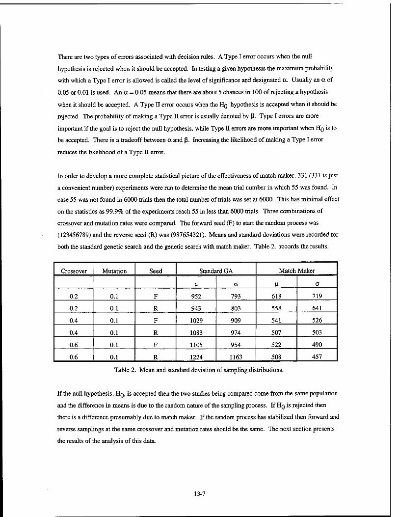
There are two types of errors associated with decision rules. A Type I error occurs when the null

hypothesis is rejected when it should be accepted. In testing a given hypothesis the maximum probability

with which a Type I error is allowed is called the level of significance and designated a. Usually an a of

0.05 or 0.01 is used. An a = 0.05 means that there are about 5 chances in 100 of rejecting a hypothesis

when it should be accepted. A Type II error occurs when the HQ hypothesis is accepted when it should be

rejected. The probability of making a Type II error is usually denoted by ß. Type I errors are more

important if the goal is to reject the null hypothesis, while Type II errors are more important when HQ is to

be accepted. There is a tradeoff between a and ß. Increasing the likelihood of making a Type I error

reduces the likelihood of a Type II error.

In order to develop a more complete statistical picture of the effectiveness of match maker, 331 (331 is just

a convenient number) experiments were run to determine the mean trial number in which 55 was found. In

case 55 was not found in 6000 trials then the total number of trials was set at 6000. This has minimal effect

on the statistics as 99.9% of the experiments reach 55 in less than 6000 trials. Three combinations of

crossover and mutation rates were compared. The forward seed (F) to start the random process was

(123456789) and the reverse seed (R) was (987654321). Means and standard deviations were recorded for

both the standard genetic search and the genetic search with match maker. Table 2. records the results.

Crossover Mutation Seed Standard GA Match Maker

M- a H a

0.2 0.1 F 952 793 618 719

0.2 0.1 R 943 803 558 641

0.4 0.1 F 1029 909 541 526

0.4 0.1 R 1083 974 507 503

0.6 0.1 F 1105 954 522 490

0.6 0.1 R 1224 1163 508 457

Table 2. Mean and standard deviation of sampling distributions.

If the null hypothesis, HQ, is accepted then the two studies being compared come from the same population

and the difference in means is due to the random nature of the sampling process. If HQ is rejected then

there is a difference presumably due to match maker. If the random process has stabilized then forward and

reverse samplings at the same crossover and mutation rates should be the same. The next section presents

the results of the analysis of this data.

13-7

6. Analysis of the Statistical Data

The following paragraphs give results of the analysis of the data collected in section 5. The data was tested

at the 0.05 significance level which means that HQ is not rejected if the normalized variable z is Izl < 1.96

and is rejected if Izl > 1.96 for a two-tailed test. To preview the results, each sample collected with the same

crossover and mutation rates tested from the same distribution regardless of forward or reverse seed. This

indicates that the 331 samples is enough to make the process independent of the starting seed. A

comparison of samples under identical conditions, except for match maker, shows that the samples come

from very different populations and that the results are highly significant.

Crossover 0.2 Mutation 0.1

Comparison of forward and reverse seeds without match maker.

z = 0.14 Samples from same distribution, process independent of seed. Because the

means are so close the chance of accepting the null hypothesis when the means come

from different populations is quite high, ß for z = 0.14 is 0.9434 when a is 0.05. If a is

relaxed then ß can be reduced.

Comparison of forward and reverse seeds with match maker.

z = 1.15 Samples from same distribution, process independent of seed but the conclusion

is not as clear cut as above, ß is 0.79. Because the separation of the means is greater than

above the chance of accepting the null hypothesis when it should be rejected is less.

Comparison of forward seeds with and without match maker.

z = 7.38 Samples clearly from different distributions. At this level of

significance there is very little chance of error.

Comparison of reverse seeds with and without match maker,

z = 6.83 Samples clearly from different distributions.



z = 0.734 Accept HQ. The samples probably come from the same

distribution, ß is 0.8715.


z = 0.865 Samples from same distribution, process independent of

seed, ß is 0.8619.


z = 8.44 Samples clearly from different distributions. At this level of

significance there is very little chance of error.

13-8

Comparison of reverse seeds with and without match maker,




z = 1.44 Accept HQ. The samples probably come from the same

distribution, ß is 0.699.


z = 0.372 Samples from same distribution, process independent of

seed, ß is 0.9342.



Comparison of reverse seeds with and without match maker.


7. Conclusions

It is concluded that match maker has an effect, that the results are not statistical variations of the sampling

process and that match maker favorably impacts the process. Thus match maker makes an important

improvement in the convergence rate for this problem. Match maker should undergo further testing to see if

it can also improve the convergence rate in other, more difficult problems. If it can, then, match maker can

be an important contribution to genetic algorithms.

References

M. L. Cone (1995). A genetic algorithm scheduler for the sensor manager. In USAF Summer Research Extension Program. RDL: Culver City, CA.

J. J. Grefenstette, L. Davis, & D. Cerys (1991). GENSIS and OOGA: Two Genetic Algorithm Systems. TSP, Melrose, MA.

M. R. Spiegel (1988). Schaum's Statistics. McGraw-Hill, New York

13-9

Metrics

1. Introduction

The purpose of this paper is to look at classic metrics to see which are appropriate for evaluating the sensor

manager's schedule. The metric dictates to some extent the kind of scheduler that is appropriate since for

some metrics there are optimal dispatch rules that can be used and for others a heuristic scheduling

approach may be known only for certain metrics. The paper starts with an overview of the sensor manager

scheduling problem. Next several classic metrics that have been used to develop schedules are summarized.

An evaluation of some of the metrics versus the sensor manager's scheduling problem follows. Finally,

examples showing the impact of different metrics on the similar job shop scheduling problem are given,

followed by conclusions.

2. The sensor manager's scheduling problem

Aspects of the scheduling problem have been summarized by [Popoli, 1992]. He lists the following

problems that the sensor manager might have to deal with:

• There are hard deadline tasks that have to be completed in a narrow window if they are to be of

any value.

• There are tasks without deadlines that have earliest start times before which they can't begin

execution.

• There are differences in task priorities. Some tasks are very important, others routine. A task's

priority generally reflects the urgency of its start time.

• Some tasks may be interruptable, others not.

• Tasks may vary greatly in length.

• Tasks can become necessary or unnecessary very suddenly.

• There may be some uncertainty in the requirements for the task. For example, the duration of

the task may not be known when the task begins execution.

Other problems not mentioned by Popoli include:

• Sensors may need to operate in parallel. At times one of the parallel tasks may be a no-op

effectively keeping one sensor from interfering with the operation of another sensor.

• Sensors may need to operate in series so that one sensor can cross queue another. This task

requires sequential operation of two or more sensors with possibly slack time between operations

to allow data to be transferred between sensors.

• The plant may change while the scheduler is operating. Some sensors may become inoperable

requiring an emergency rescheduling.

13-10

• Workload can be heavy requiring efficient use of all resources.

3. Classic Metrics

Unless noted these metrics come from [Penedo, 1995]. Generally the goal of the scheduler is to minimize

the value of these metrics (also called objective functions).

Makespan (Cmax). Makespan is the maximum of the completion times of the jobs in the system. It is the

time when the last job finishes. By minimizing the makespan jobs get through the system faster which leads

to better utilization of the machines.

Total weighted completion time (XWJC;). Completion time is taken as the time when a job finishes. It is

not referenced to when the job starts. Total weighted completion time measures how long it takes to

process the n jobs that the sum runs over. A longer weighted completion time means that there is more

work-in-process (WIP) in the plant. The weights account for different inventory costs while the material to

produce the products is in the plant. The sum of the completion times is also known as the flow time and

this metric may also be called the weighted flow time. A variation of this metric involves squaring the

completion time and adding a weight leading to the weighted sum of squared completion time metric.

Maximum lateness (Lmax). Lateness is the difference in time between the time when the job actually

completes and the due date for the completion of a job. Positive lateness means the job finished late and

negative lateness means the job finished early. The goal is to minimize the lateness of the worst job.

Lateness relates to customer satisfaction and is not appropriate when the jobs do not have deadlines. If all

jobs in the problem have a common deadline, then minimizing maximum lateness is the same as minimizing

makespan. Two variants of lateness are total lateness, the sum of the lateness for each job, and total

weighted lateness which applies a weight to each job's lateness.

Total weighted tardiness (EWJTJ). Tardiness is the maximum of lateness or 0. It recognizes that in some

cases there are penalties for being late but no benefits for being early. The total weighted tardiness sums the

tardiness for each job in the n jobs being considered in this planning cycle. Jobs must have deadlines for

this metric to be useful. Other variations on this same theme include letting all of the weights equal 1, only

considering the maximum tardiness or summing the weighted tardiness squared (ZWJTJ2

).

Weighted number of tardy jobs (XwjUj). U; is either one or zero. If the weights are all one then the

weighted number of tardy jobs is just the number of tardy jobs. This measure is simple to collect and

13-11

understand so is frequently used in practice. It is a measure of total customer satisfaction but is not

sensitive to how mad customers might be if their jobs are very late.

Sequence dependent setup times (Esp). Sjjjj is the sequence dependent setup time between job j and job k

for machine i. Minimizing this measure increases throughput and decreases slack time between jobs.

Idleness (SIj). Idleness is the time between the finish and the start of a job that is not devoted to

processing. It includes the dead time when the jobs are waiting to get on a machine and the sequence

dependent setup times. It is computed by taking the completion time of a job and subtracting the start time

and all of the time devoted to processing. Idleness is also known as slack time.

Economic makespan (XR^Cj^-a^)). The economic makespan metric [Morton and Pentico, 1993] builds

schedules that reflect the cost of machine utilization. A price, R^, is estimated for running the machine.

This price is multiplied times the completion time, C^, of the last job on that machine minus the earliest

time, a^, that the machine is available. This objective function is good in a heavily loaded shop where new

jobs are always coming in so that the idle time at the end of the current planning horizon for a particular

machine can be filled by the new jobs. It is generally equivalent to minimizing the internal slack in the

system.

Discounted total weighted completion time (SwjCl-e"1^;)). In the discounted total weighted completion

time the jobs that take longer to complete contribute a larger percentage of their weight, w;, to the metric.

As a measure, it favors finishing the longer jobs at the cost of taking longer to do the shorter jobs.

Total weighted earliness (SßiEj2). [Czerwinski and Luh, 1994] estimate the theoretical part start date by

backtracking along the critical path from the due date. Earliness is defined as the time ahead of the

theoretical part start date that the part actually starts production. There is no penalty for starting after the

theoretical start date. Squaring the earliness function causes the penalty to increase faster the larger

earliness becomes.

Number of processors (n). If there are more machines available then jobs then this schedule tries to

minimize n, the number of machines used. This objective function is usually associated with a shop that has

several identical machines operating in parallel.

13-12

4. Discussion of individual metrics

Makespan is probably the most frequently used metric for schedule generation. [Kober, 1994] has

suggested that some metric other than makespan may have some value for the sensor manager scheduler.

[Stankovic, et. al., 1995] believes that makespan is important in that it minimizes required system resources

but since it does not directly address deadlines it can't be a primary metric. Stankovic maintains that for

real-time systems the sum of completion times is not important because it doesn't have a direct assessment

of timing properties like deadlines and periods. He sees value in the weighted sum of completion times

since it recognizes that some jobs have more value than others. He also feels that value and deadlines are

both important and that many real-time scheduling systems concentrate only on deadlines.

Minimizing maximum lateness doesn't prevent tasks from being late. It is possible to construct an example

that minimizes the maximum lateness yet has all tasks miss their deadlines, [Stankovic, et. al., 1995].

Optimizing the total lateness or total weighted lateness may help but it also might cause more tasks to miss

their deadlines while trying to reduce the lateness of a very tardy task. Tardiness has the same problem as

lateness. By itself it isn't sensitive to the number of late jobs. For a real-time operation, being on time is the

most important measure of the effectiveness of a schedule. Minimizing the number of tardy jobs or the

weighted number of tardy jobs helps correct this. However, since the sensor manager is dealing with a task

set that may contain many jobs without deadlines, in cases where processor utilization is equally important,

objective functions that are only sensitive to deadlines are not totally adequate.

Minimizing either sequence dependent setup times or idleness is a direct measure of throughput through the

system. While these metrics increase efficiency they do not directly assess a schedule's ability to meet

deadlines.

The total weighted earliness metric penalizes a job for starting early. The presumption here is that jobs that

start too early end up staying in the plant too long which increases the work-in-process (WIP) costs. This

metric is generally used in conjunction with a metric that senses completion time so that the job has a

window of opportunity in which to move through the plant.

The economic makespan is similar to idleness except that idleness is based on how long jobs set idle

whereas economic makespan is based on how long machines are idle. Like several of the other metrics, it

has no sense of which jobs need to be completed to meet deadlines. Plant efficiency may have to be

sacrificed in order to complete certain jobs on time. This metric has the distinction of including a weight

measuring the importance of each machine. For example, the IR system may be favored over the radar in

low emission modes so the weight of the IR sensor may be high in certain periods of the mission.

13-13

The discounted total weighted completion time evaluation function produces schedules that improves plant

efficiency by scheduling longer and more important jobs first. Schedules generated from this metric are

similar to those using the longest processing time first dispatch rule. The difference is that the discounted

total weighted completion time metric includes slack time. This metric is useful to the sensor manager only

if another metric is included which measures the ability of the schedule to meet deadlines.

The last metric, number of processors, is not particularly useful for the sensor manager. It is appropriate

when there are several jobs and several machines available to choose from, and the jobs can run in parallel.

As this is not the usual sensor manager architecture the number of processors metric would not be

appropriate.

For a dynamic scheduling algorithm (one that schedules tasks when they arrive and the arrival times are

unknown in advance to the scheduler) the choice usually goes to a metric for which an optimal dispatch rule

is known. These rules generally exist only for standard plant models which the sensor manager architecture

will probably not match. For example there are dispatch rules such as "weighted shortest processing time

first" when all release dates and due dates are 0 or "earliest due date first" when all due dates are

sufficiently loose and spread out, that optimize the weighted tardiness under certain very restrictive

conditions. While these dispatch rules may not be appropriate for the configuration the sensor manager

finds itself in, they can still be used to make schedules for the initial population.

The next section considers the effect of combining individual metrics to improve the performance of the

schedules.

5. Evaluation of combined metrics

Metrics generally fall into two classes. The first deals with a schedule's ability to meet its deadlines.

Lateness, tardiness, number of tardy jobs and their variants belong to this class. The second group of

objective functions measures some aspect of processor utilization. Makespan, economic makespan,

completion time, sequence dependent setup times, earliness, number of processors and their variants are

examples. A good metric should have a measure from each class if it is to address the needs of real-time

scheduling.

Penedo suggests that one particular combination of objectives used in the process industry is the

minimization of total weighted tardiness and the sum of sequence-dependent setup times. Weighted

tardiness measures a company's ability to maintain the quality of its service while the sum of sequence-

dependent setup times indirectly measures the plant's efficiency (throughput). The relative importance of

13-14

the two may change over time. When the workload is light, tardiness may be more important, but when the

workload is heavy, plant efficiency may be more important.

[Czerwinski and Luh, 1994] also use a combined objective function in their Lagrangian relaxation

technique. This one combines an earliness with a tardiness penalty. These penalties together define a time

interval in which an operation can be scheduled with zero penalty. The objective of this penalty function is

to ensure on-time part completion and low work-in-process inventory. By penalizing schedules that start

early, machine utilization is improved and slack time is reduced.

The next two subsections evaluate the Pinedo and CzerwinskiTLuh combined metrics ability to handle the

sensor manager's scheduling problem.

5.1 Pinedo pair discussion

Schedules produced by the Pinedo pair, total weighted tardiness and the sum of sequence-dependent setup

times will be evaluated as to its ability to solve the sensor manager's scheduling problems of Section 2.

Hard deadlines that have earliest start times use both metrics to define an operating window in which they

can operate. The weighting factor takes care of any differences in the tasks' priorities. While the metrics do

not directly address whether the tasks are interruptable, any task that is can be tested against the metric to

see if it produces a better schedule. Varying task length does not directly impact the metric evaluation.

Sudden changes in a task's priority require a separate mechanism in the scheduler which is not a function of

the metric. For example, a pop-up job may be handled by a separate reactive scheduler [Morton & Pentico,

1993]. The reactive scheduler tries to produce a feasible schedule that has a minimal impact on the current

working schedule. It may not use a metric at all and may be as simple as trying to fit the task into a space in

the existing schedule or delaying tasks on a machine by enough to fit in the pop-up job. Reactive

schedulers have to be fast. If a new schedule can be built in time to handle the pop-up task using the usual

scheduling cycle, then there is no need for a reactive scheduler. The Pinedo pair, while not taking much

longer than any other metric, probably takes too long to be considered for reactive use.

Uncertainty in task requirements means that there is some information that is needed for scheduling that is

not precisely known. Whatever uncertainty there is gets mapped into uncertainty in the objective function.

It then becomes a matter for the scheduling algorithm to manage that uncertainty. Under some conditions

there are some NP-hard problems for deterministic models that have known optimal solutions for stochastic

models. One of these results is for the single machine problem when all deadlines are equal and the metric

is the sum of the weighted tardiness. This may be useful information to the scheduling algorithm whenever

the Pinedo pair is chosen.

13-15

The next two bullets from Section 2. concern sensor architecture, the modeling of the sensors in series or

parallel or a combination of both (job or flow shops). Sensor architecture only affects the Pinedo pair in

that there are limited configurations and conditions for which optimal scheduling algorithms are known. In

particular, one metric of the Pinedo pair, the sum of weighted tardiness, is NP-hard in the strong sense even

for one machine. This means that it is unlikely that a general algorithm can be found that gives an optimal

schedule in polynomial time and suggests that a heuristic scheduling technique like genetic search or

Lagrangian relaxation is required to develop good schedules.

The next problem, plant change, really doesn't affect the Pinedo pair. For example, if one sensor goes off-

line while the schedule is operating, the scheduler may have to go into a short rescheduling sequence using

a less demanding metric. This is the same as letting the reactive scheduler take over for the short term

before transitioning back into the long range scheduler.

Heavy workload presents its own problems. The ideal schedule is one that has the plant working at peak

efficiency. The weighted sum of tardiness is appropriate under heavy workload conditions since it allows

the most important jobs to be scheduled first and less important jobs to be left to later. Minimizing the

setup times reduces sensor idle time which helps throughput when the workload is heavy. The setup times

metric may not be as appropriate as makespan or economic makespan which more directly address

processor utilization.

5.2 Czerwinski and Luh discussion

The Czerwinski and Luh metric combines tardiness and earliness penalties for operations. They use the

following formula summed over all jobs:

Z(wjTj2 + ßjEj2)

In their formulation, the squaring of the tardiness and earliness metric penalizes the later or earlier jobs

more. This metric seems to be superior to the Pinedo pair against the first criteria, hard deadlines. While it

forces jobs into a window of opportunity which is what the first bullet requires, it also works directly on the

second bullet which requires jobs to start after a certain time. This metric is superior to Pinedo on this point

as Pinedo addresses the start time only as a second order effect. A possible problem with the

Czerwinski/Luh metric is that if some of the start times can't be violated, this objective function penalizes

but does not prevent jobs from starting early. As with Pinedo, weighting takes care of differing task

priorities.

13-16

The Czerwinski and Luh metric has no known optimal dispatch rule for any interruptable system (or for any

system for that matter). This means that a heuristic is required to develop schedules. Varying length

schedules pose no problem for the metric. Pop-up jobs have to be handled by a reactive scheduler as was

done for Pinedo. Uncertainty in the knowledge of start times for due dates is reflected in uncertainty in the

evaluation of a schedule. The Pinedo pair may have an advantage here since the setup times should be

determined in advance and the type of job to be scheduled has to be known as a minimum. Thus it is likely

there are less unknowns in the Pinedo pair.

The other problems that the scheduler may have to handle are similar for both metric combinations with the

exception of the last bullet which is heavy workload. By squaring the tardiness and earliness penalties,

Czerwinski and Luh get a tighter control of throughput and should be able to develop schedules that make

more efficient use of the sensors.

5.3 Recommendation

Inclusion of both classes of metrics is needed to produce a balanced result and so the recommendation is to

choose one metric from each class and build schedules using the combined metric. Which metrics to use

depend on the details of the avionics architecture used for the sensor suites and may vary with the intended

mission. Of the two combined metrics considered, the Czerwinski and Luh combination seems a better

choice.

6. Comparison of Example Schedules Generated by Different Metrics

As a simple demonstration of the impact of metrics on schedules, consider the 6x6 job shop scheduling

problem (JSSP), [Muth & Thompson, 1963]. In the 6x6 JSSP there are 6 machines and 6 jobs. Each job is

processed on all six machines but each in a different order. Three schedules were generated using different

evaluation functions. The three metrics used were makespan, sum of squared completion times and a

combination of makespan and sum of squared completion times. An evaluation of 55 is the known optimal

solution for makespan and is easily found by the genetic algorithm (GA). One of the many schedules with a

makespan of 55 was chosen to evaluate the sum of squared completion times. The sum of squared

completion times takes the time when each of the six jobs in the 6x6 JSSP completes, squares the

completion times and adds them. If the due date for each job is 0 then the completion date is the same as

the tardiness and the sum of squared completion times is the same as the sum of squared tardiness. Table 1.

lists the makespan and sum of squared completion times for all three schedules. The schedules in Table 1.

are individual schedules arbitrarily chosen from the list of those schedules minimizing their performance

metric.

13-17

Measure of Performance Schedule Evaluation Function

Makespan Squared Completion Combined

Makespan 55 64 60

Squared Completion 15607 13191 13298

End Time

Jobl 48 26 26

Job 2 52 64 60

Job 3 55 56 56

Job 4 54 59 58

Job 5 53 29 29

Job 6 43 31 41

Idle Time 108 68 73

Table 1. Comparison of schedules produced by three different metrics.

The makespan schedule found the optimal value of makespan but at the expense of the sum of completion

times squared. Looking at the end times of the jobs, the makespan metric tends to balance the completion

times of all jobs. There is no premium for completing jobs early. On the other hand, the sum of squared

completion times tries to complete jobs as soon as possible. If the environment is such that machines set

idle after a job is done waiting for the next surge, then makespan is a better metric since the last of the jobs

completes earlier and the next sequence can start sooner. If there are jobs coming in that could be

scheduled on a machine when it is available then the sum of squared completion times finishes some jobs

early and frees the machines for new jobs. For example, job 1 finishes at 48 for the makespan schedule, but

at 26 for the sum of squared completion times. If there are new jobs that could use machine 1 but are not in

the original schedule, then they could start at 26 with the squared completion times schedule. Job 5 shows

similar results.

The third metric combines makespan and squared completion times. The makespan is squared in order to

get the units of makespan the same as squared completion times. The result is a compromise between the

makespan and squared completion time schedules. Compared to the previous schedules, the makespan is

about half-way between and the sum of squared completion times is nearly as good as the sum of squared

completion time schedule.

Another way to compare schedules is on the basis of idle or slack time (defined as the completion time

minus the actual total time on all machines required for a job). For example, job 1 on the makespan

13-18

schedule completes at 48. If it is scheduled without any other jobs it would take 26 units to complete by

going directly from one processor to another. Thus job 1 sets idle for 22 units sometime during its

processing. Table 1. shows the idle time for each schedule. For these schedules the sum of squared

completion times produces a schedule that has the machines setting idle for the least time, although the

combined metric does almost as well.

As another example, consider the schedules produced by the dispatch rules, shortest processing time (SPT)

first and longest processing time first (LPT). In SPT the job with shortest execution time which has an open

machine and has its previous task completed is run next. LPT is the same as SPT except the job with the

longest processing time is considered first. The SPT rule is optimal for a flow shop where each of m

machines are in series, every job must be processed on every machine, each machine takes the same amount

of time to process job;', and the criteria is to minimize makespan. LPT optimizes makespan on m parallel

machines by assigning the m longest jobs to the m machines. After that, whenever a machine is freed, the

longest unscheduled job is put on that machine. Table 2. shows the results of the SPT and LPT rules

applied to the JSSP.

Measure of Performance Schedule Evaluation Function

SPT LPT

Makespan 84 76

Squared Completion 19507 21506

End Time

Jobl 38 70

Job 2 84 53

Job 3 50 49

Job 4 41 52

Job 5 51 54

Job 6 65 76

Idle Time 132 158

Table 2. Schedules produced by dispatch rules.

SPT doesn't produce a particularly good schedule for either of the two metrics considered here. The LPT

rule does even worse. Jobs take longer and set idle more than with any of the previous schedules. This

example illustrates the trouble with most dispatch rules when used in situations different than those in which

they were designed to operate. Performance is generally poor.

13-19

7. Conclusions

This paper has examined the impact of metrics on schedules. The sensor manager's scheduling problem was

described. Several classic metrics were listed along with the intended performance goal of the metric. It

was suggested that metrics generally fall into two classes and that a good schedule could be built by taking a

metric out of each class. Two combined metrics were evaluated as to their suitability for the sensor

manager problem. Examples of schedules built by three different metrics: makespan, sum of squared

completion times and a combination of both metrics were presented. They were evaluated based on the

makespan and sum of squared completion times metrics and also by a third metric, idleness, that none of the

schedules were designed to optimize. Finally two common dispatch rules, SPT and LPT, were used to

produce schedules that were based on the three previous metrics.

As expected, a schedule that is tuned to one metric generally performs poorly in a different metric. Thus

the sensor manager problem needs to be carefully analyzed so that the right metric is chosen. The schedule

generated by the combined makespan and sum of squared completion times was a compromise between the

schedules produced by the individual metrics. If the due dates of all jobs are considered to be the beginning

of the scheduling period, then the sum of squared completion times is the same as squared tardiness and the

combined metric example is an example of a metric taken from each class. The result is a schedule that

combines features of each of the individual metrics to produce a good schedule but not one that maximizes

the performance of any one individual metric.

References

C. S. Czerwinski & P. B. Luh (1994). Scheduling products with bills of materials using an improved lagrangian relaxation technique. IEEE Trans on Robotics and Automation, Apr.

W. Kober (1994). Personal communication.

T. E. Morton & D. W. Pentico (1993). Heuristic Scheduling Systems. John Wiley and Sons, Inc, New York.

J. F. Muth & G. L. Thompson (1963). Industrial Scheduling. Prentice Hall, Englewood Cliffs, NJ.

M. Pinedo (1995). Scheduling Theory, Algorithms, and Systems. Prentice Hall, Englewood Cliffs, NJ.

R. Popoli (1992). The sensor management imperative. In Yaakov Bar-Shalom, editor, Multitarget- Multisensor Tracking: Applications and Advances Volume II. Artec House, Norwood, MA.

J. A. Stankovic, M. Spuri, M. Di Natale, & G. C. Buttazzo (1995). Implications of classical scheduling results for real-time systems. Computer, Jun.

13-20

OPTICAL STUDIES OF TWO NOVEL ELECTRO-EXPLOSIVE DEVICES

Robert R. Criss Assistant Professor

Department of Physics

Randolph-Macon Woman's College 2500 Rivermont Avenue

Lynchburg, VA 24503-1526

Final Report for: Summer Faculty Research Program Wright Laboratory, Eglin AFB, FL



and

Wright Laboratory, Eglin AFB, FL

July 1996

14-1


Robert R. Criss Assistant Professor

Department of Physics Randolph-Macon Woman's College

Abstract

High speed streak photography and time integrated spectroscopy were used to characterize optical

emissions from plasmas formed by two novel electro-explosive devices; a semiconductor bridge (SCB), and a

semiconductor junction igniter (SJI). The spatial extent and expansion velocity of each plasma were determined as a

function of time. An estimation of ion/neutral temperature was made by assuming that the identity of the

ion/neutral was known and that the plasma was expanding freely in the plane parallel to the plane of the device. Time

integrated spectra of the plasmas were complex and analysis is not complete at this time.

14-2


Robert R. Criss

Introduction

Semiconductor bridges (SCB's) and semiconductor junction igniter's (SJI's) are electro-explosive devices

used to provide ignition of energetic compounds such as pyrotechnics and propellants. They can be used in

products ranging from automotive airbags to ordinance systems. The detailed structure of these devices has been

published elsewhere and will not be discussed in this report.1"2 A current pulse applied to the SCB/SJI quickly heats

the device, producing an ionized plasma which is used to ignite an energetic compound. Though the exact

mechanisms responsible for ignition are unknown, one might reasonably expect them to be related to plasma

properties such as the identity of species, temperature, density, expansion velocity, and amount of ionization. A

study of optical emissions from the plasma, taken in conjunction with current-voltage measurements, offers the

promise of determining all of the aforementioned plasma properties. Our optical studies consisted of high speed

streak photography and time integrated, multichannel emission spectroscopy. A preliminary analysis of the results is

presented in this report.

Methodology

The procedures used to collect data were the same for both SCB and SJI devices. All of the devices were

fired with a current pulse from a 0.2/iF capacitor charged to lkV. Multiple SCB's (and SJI's) were necessary to collect

a complete data set Since the I-V measurements from all of the SCB's were nearly identical, it has been assumed

that the plasma properties were reproducible from shot to shot This was also the case for the SJI's.

A bi-convex lens was used to focus an image of the device onto the entrance slit of the streak camera. Streak

pictures (covering a 2/*s time interval) of the luminous plasma were taken with the plane of the device parallel to the

plane of the camera entrance slit (front view) and with the plane of the device perpendicular to the plane of the

camera entrance slit (side view). Intensity contours from pictures taken with the device in each orientation

determine the location of the luminous plasma as a function of time. An intensity contour from the front view

pictures was used to determine the extent of the luminous plasma in the plane parallel to the plane of the device as a

function of time. When this location is plotted against the time, the slope of the curve yields the parallel expansion

14-3

velocity (this is the velocity of the plasma in the plane parallel to the plane of the device). Likewise, pictures taken

from the side view yield, as a function of time, the extent of the luminous plasma in the plane perpendicular to the

device and the perpendicular expansion velocity.

Spectra were collected with a 1-dimensional, computer interfaced diode array coupled to the exit of a

grating spectrometer. Each device was aligned with the plane of the device parallel to the plane of the spectrometer

entrance slit Spectra were collected from 200nm to 700nm in intervals of approximately lOOnm.

Results

Typical front and side view streak pictures of the plasma formed by an SCB are shown in figure 1. A contour

was traced along the edge of each picture and, from this contour, data points were taken for the plots of the spatial

extent of the SCB plasma as a function of time, shown in figure 2. Sixth order polynomials were fit to each curve.

The derivatives were then used to generate plots of the instantaneous expansion velocities as a function of time,

shown in figure 3. If the expansion of the plasma is assumed to be a free expansion, and if the identity of the plasma

species is known, the equipartition of energy theorem can be used to estimate the plasma ion/neutral temperature.

Under these conditions, the temperature can be written as

T = mv2/3k . (1)

where T is the temperature, m is the mass of the plasma species, k is Boltzmann's constant, and v is the velocity.

Aluminum and silicon are the species present in the plasma (this conclusion can be drawn from knowledge of device

construction and confirmed spectroscopically). The condition of 'free expansion' would most likely be met for

plasma expansion in the plane parallel to the plane of the device and at some time after the initial burst of plasma

formation. Using the parallel expansion velocity of the SCB plasma at a time 0.2 /AS after the initial burst yields a

temperature of 693 K for an aluminum plasma and 720 K for a silicon plasma. A volume of 0.09 mm3 was

calculated for the plasma at this time(0.2 its) by using the equation for the volume of a right circular cone and

dimensions taken from figure 2.

Typical front and side view streak pictures of the plasma formed by an SJI are shown in figure 4. Plots of the

spatial extent of the SJI plasma and the instantaneous expansion velocities, generated by the procedure outlined

above, are shown in figures 5 and 6. Substituting the parallel expansion velocity of the SJI plasma at a time 0.2 /xs

after the initial burst into equation (1) yields a temperature of 1309 K for an aluminum plasma and 1362 K for a

14-4

Silicon plasma. A volume of 0.19 mm3 was calculated for the plasma at this time(0.2 fis) by using the equation for

the volume of a right circular cone and dimensions taken from figure 5.

Spectra collected from both devices should confirm the identification of species in the plasma and might be

suitable for determination of the plasma electron temperature. The analysis has not been completed at this time but

will be presented for publication at a later date. Values for the resistivity, calculated from the current-voltage traces,

might also be used in conjunction with this temperature to determine the fractional ionization of the plasma.

Summary & Conclusions

Streak photography has been used to determine the location and expansion velocity of luminous plasmas

from SCB and SJI devices. Expansion velocities were measured both parallel and perpendicular to the plane of the

device. In each case, the velocity started at a maximum and decreased most sharply in the first O.ljtiS of the plasma

discharge. For both devices, the initial parallel expansion velocity was slightly larger than the initial perpendicular

expansion velocity. This may be due to shock effects or errors in alignment of the device with the streak camera slit

The effect of contrast enhancement of the streak pictures on the results of the image analysis also needs to be

considered. Further data analysis, which includes the consideration of shock effects, should resolve questions about

the validity of the temperature measurement discussed in this report

Though not presented in this report, analysis of the spectral data is ongoing. A tentative summary of those

results is presented in this report Spectral emissions from aluminum and silicon have been identified. It seems

possible that at least some of the features appearing in the spectra are from the air surrounding the plasma discharge.

Calculations of the plasma density as a function of time should suggest at what stage of the discharge features from

the surrounding air would be expected to appear. Spectra collected when the device is in a vacuum could also assist

in the identification of spectral peaks. It should be noted that all of the spectra collected were integrated, in time,

over the full duration of the plasma discharge.

We are still at too early a stage of data analysis to compare the results from the measurements on SCB

plasmas to those on SJI plasmas. Indeed, most of the analysis not yet complete. An ion/neutral temperature and an

estimation of plasma density should be possible from the streak pictures, used in conjunction with knowledge of

device geometry and some reasonable assumptions. The spectra have already confirmed the presence of aluminum

and silicon in the plasma. It might be possible to calculate a temperature, approximating the electron temperature,

14-5

from the spectra. If so, this temperature could be used in conjunction with the plasma resistivity (taken from the I-V

curves) to estimate the fractional ionization of the plasma. The complete analysis will be submitted for publication

in professional journals at a later date.

References

1. D. A. Benson, M. E. Larsen, A. M. Renlund, W. M. Trott, and R. W. Bickes, Jr. ,J. Appl. Phy. 62(5), 1622

(1987).

2. Thomas A. Baginski, IEEE Trans. Ind. App. 29(2), 412 (1993).

14-6

SCB: Position of Luminous Perpendicular Expansion Front

0.60 -i

0.50 —

0.40 —

E E § 0.30

"5 o 0.

0.20

0.10

0.00 —>

I ' I ' I ' I ' I ' I ' I ' I ' I ' I 0.00 0.10 0.20 0.30 0.40 0.50 0.60 0.70 0.80 0.9O

Time (us)

SCB : Position of Luminous Parallel Expansion Front

0.70 —i

i i r~^n ' i r—r^ i ' i ' i—>—i 0.00 0.10 0.20 0.30 0.40 0.50 0.60 0.70 0.80

Time (us)

Figure 2. 14-8

SCB: Perpendicular Velocity

5.00

4.00

CO 3 son C" e 2- o o <B 700 >

1.00

0.00

0.00 0.10 ~i—■ r~ 0.20 0.30

Time (us) 0.40 0.50

SCB: Parallel Velocity

E

s o

10.00

9.00

8.00

7.00

6.00

5.00

4.00

3.00 —

2.00 —

1.00 —

0.00

0.00 0.10 0.20 Time (us)

0.30 0.40

Figure 3. 14-9

SJI: Position of Luminous Perpendicular Expansion Front

0.90 —i

0.80 —

0.70 —

0.60 —

E E 0.50 —

55 0.40 -\ o a.

0.30

0.20

0.10

0.00 —! I ' I ' I ' I ' I ' I ' I ' I ' I ' I

0.00 0.10 0.20 0.30 0.40 0.50 0.60 0.70 0.80 0.90 Time (us)

0.70 —i

0.60

0.50

0.40 —

c

g 0.30 O.

0.20 —

0.10 —

SJI: Position of Luminous Parallel Expansion Front

-K

0.00 —' + + I ' I ' I ' I ' I ' I ' I ' I ' I ' I

0.00 0.10 0.20 0.30 0.40 0.50 0.60 0.70 0.80 0.90 Time (us)

Figure 5. 14-11

SJI: Perpendicular Velocity

7.00

6.00

5.00 —

g 4.00 —

o 3.00

2 2.00 —

1.00 —

0.00

i ' i ' r~ 0.00 0.10 0.20

n—'—r~ 0.30 0.40

Time (us) 0.50

SJI: Parallel Velocity

7.00

6.00 —

5.00

4.00

O 3.00

2 2.00

1.00

0.00

0.60 0.70

i ' i ' i ' i—' r~ 0.00 0.10 0.20 0.30 0.40 0.50

Time (us)

Figure 6. 14-12

GRAIN SIZE EFFECTS IN THE DETERMINATION OF

X-RAY POLE FIGURES AND

ORIENTATION DISTRIBUTION FUNCTIONS

Robert J. De Angelis Professor

Department of Mechanical Engineering

University of Nebraska-Lincoln 255 Walter Scott Engineering Center

Lincoln, Nebraska 68588-0656


Wright Laboratory Eglin Air Force Base, FL 32542



and

Wright Laboratory Eglin Air Force Base, FL

15-1

August 1996

GRAIN SIZE EFFECTS IN THE DETERMINATION OF

X-RAY POLE FIGURES AND


by: Robert J. De Angelis

Department of Mechanical Engineering University of Nebraska-Lincoln Lincoln, Nebraska 68588-0656

Abstract

The production of metallic materials with controlled degrees of anisotropy is important

because the controlled texture provides significant assurance that subsequent plastic

deformation can be performed successfully and reproducibly. To proceed to this condition,

the degree of anisotropy must be quantified by the experimental determination of x-ray pole

figures and the orientation distribution functions (ODF) calculated from the pole figure data.

To insure the intensity data collected is reliable the grain size of the specimen must be suitably

small. The objective of this research was to determine the grain size error in measurement of

pole figures on the x-ray diffractometer at Eglin AFB.

15-2

GRAIN SIZE EFFECTS IN THE DETERMINATION

OF

X-RAY POLE FIGURES

AND


Robert J. De Angelis

Introduction

Since the 1980's the description of material textures or crystal orientations in polycrystalline

wires and sheets started to move beyond the x-ray determined pole figures, the norm since the

1930's. The orientation distribution function (ODF) has recently become the method of choice

for presenting the description of material textures. This change was driven by the need for a

more complete method of describing and quantifying textures in the tailor making of materials

and was made possible by the advances in computer speed and capacity. The ODF is

computed from pole density data usually represented on pole figure plots which give the

density of poles (normals to a crystallographic plane) of a specific {hkl} plane in units of

multiples of the random pole density for that particular {hkl} pole. Pole figures are usually

15-3

represented on two dimensional polar coordinate plots where the center of the pole figure is the

normal to the sheet surface and the direction to the right is parallel to the rolling direction.

Therefore it is clear that the pole figure gives the position of the orientation of the specified

{hid} poles relative to and axial system based on the sample; e.g. rolling plane and rolling

direction in the case of sheet textures or wire axis direction in the case of wire textures. The

ODF gives the statistical distribution of crystallites in a small range of orientations plotted on

an angular axial system related to the crystallographic axis. A great advantage to the ODF

method of texture representation is that the coefficients of the harmonic equations employed to

describe the function provide weighing factors for the determination of the anisotropic elastic

and plastic properties of the material. These coefficients also are sensitive to orientation

changes that occur during certain solid state processes, such as; phase transformations, plastic

deformation and recrystallization.

However there has been little concern over the errors in measurement when

determining pole figures. There exist two contributors which determine the statistical

relevance of pole figure measurements; the number of grains irradiated in the diffraction

experiment and the photon detection. The main objective of this work is to determine the

grain size error in pole figure determinations.

Problem Description!

There is a statistical error based on the number of grain diffracting associated with the

determination of a texture pole figure. In a fixed geometry x-ray experiment the number of

grains in the beam will decrease inversely with the grain size of the diffracting material. The

error due to the number of grains diffracting is very similar to the statistical error in counting

15-4

the number of pulses arriving at a photon detector. Obviously the determination of pole

densities is a statistical process. Initially let us consider the statistical error due to photon

counting.

If many measurements of the number of photons, n, arriving at a fixed position in a

defined period of time are made. The number n will fluctuate about an average value of

counts, < n >. For a great enough number of counts (n > 100) the distribution of counts

observed follow a Gaussian distribution with a standard deviation of (n)I/2. Therefore the

counting error for one standard deviation is given by (n),/2/n or (n)",/2. For example: If <n>

is 100 counts the one standard deviation error is 0.1 or 10 counts. That is, 68% of the time

the counts observed will be between 90 and 110 counts. In practice the statistical counting

error is estimated from only one count.

Now turning to the error associated with the number of grains diffracting these same

concepts are directly applicable; i.e. the one standard deviation error in measurement is

(Nj)"1/2, where Ng is the number of grains diffracting at a fixed position. Except for a ideal

random sample the value of N, varies depending on measurement position due to type and

strength of the texture existing in the material. The most direct method to account for these

variations and evaluate the grain number error is by considering the reciprocal lattice geometry

of the powder diffraction process.

Consider the total irradiated volume of the specimen having a total of N randomly

oriented crystallites with an average volume of dv. Consider a set of (hid) planes oriented for

diffraction. The reciprocal lattice is a sphere of radius r, where the magnitude of r is l/d^.

The sphere is the locus of all normals to the (hkl) planes from all the crystallites in the

15-5

irradiated volume. The Ewald sphere intersects the reciprocal lattice sphere along a circular

line of radius (r cos (rc/2 - 6), where 0 is the perfect Bragg angle for the planes (hkl) (see Fig.

1). Very few normals, if any, that fall on the line will produce crystallites oriented for Bragg

diffraction. In a horizontal diffraction experiment the incident beam has a vertical divergence

of a. This divergence increases the contact area of the Ewald sphere and the reciprocal lattice

sphere from a line to a band of width da, as shown in Fig. 2. This immensely increases the

number of crystallites diffracting (i.e. having normals in the band on the reciprocal lattice

sphere). The fraction of crystallites diffracting at any position is given by the ratio of the area

of the band on the reciprocal lattice sphere to area of the total sphere; or:

Ng _ 2nr2cos(d-a)^ 1 - ,

-77 ^ '-da = — cosOcfa m N 4nr2 2 C1)

Introducing the multiplicity, m, of the (hkl) plane gives:

N m

N 2 (2)

In most metallic materials the diffraction process takes place in a specimen depth of dimension

much less than the grain size. Therefore it is very reasonable to employ an area rather than a

volume consideration in arriving at the number of grains available for diffraction. If a Pisson-

Voronoi mosaic basis is assumed for describing the grain size

15-6

distribution with a mean diameter d, then the average area, Ad, of a spherical grain exposed to

the beam on a fiat surface is:

Ad = d2/3.0988 (3)

Now:

N = AjJAd (4)

where At , is the area of the specimen covered by the incident beam. Then the number of

crystallites diffracting is given by:

mA. cos6<fa

*. ■ -ir (5)

The diffraction spots from these grains are spread over a cone of diffraction with an apex angle

of 40 and having a length of R, the distance from the specimen to the detector. The perimeter

of the circle containing these diffraction spots is 2 nR sin 20 at the position of the detector.

The fraction of the diffraction cone intercepted by the detector of length C is:

i/4i:Rsmd (6)

15-7

Giving the number of grains diffracting at a given position of:

n&A, da NJ = = m g 471^ sinö v/J

Resulis:

To determine the number of grains diffracting in a typical pole figure determination

experiment on a Siemens 5000 diffractometer, the following values for the quantities in Eq(7)

were employed:

height of 10 at the specimen 0.1 cm R 30 cm

9 = 22.8°

m = multiplicity = 12

{ = 1 cm

A. = 1 cm x 0.2 cm = 0.2 cm'

Ad = d2/3.0988

R = 30 cm

15-8

Inserting these quantities gives:

„/ 1.69x10-* cm 1.69xl0**(\xm)2

N* j, j, (8)

This result is shown graphically in Fig. 3 for grain sizes up to 100 microns. As can be

determined from Fig. 3 a grain size of 50 urn has a statistical error of 0.39, meaning there is a

68% probability that any measurement from this specimen where; N is 24.8 x 103 grains, N, is

914 grains and Ng' is 6.25 grains, will be from grains ranging in number from 8.95 to

3.81. Another way to look at this is, this specimen could have pole densities of between 1.39

to 0.69 times random.

REFERENCES:

H. J. Bunge, Texture Analysis in Materials Science, Butterworth, London 1982

Siemens Analytical X-ray Instruments, Inc., 6300 Enterprise Lane, Madison, WI 83719

Leonid V. Azaroff, Elements of X-ray Crystallography, McGraw Hill Book Co., New York, 1968

15-9

FIGURE CAPTIONS:

Figure 1. X-ray Powder Diffraction Geometry in Reciprocal Space.

Figure 2. The Area Sweep Out on the Reciprocal Lattice Sphere Due to Incident Beam Divergence.

Figure 3. One Standard Deviation Error in Measurement as a Function of Grian Size.

15-10

a 2

2 9

15-11

hkl Reciprocal-lattice Sphere

Figure 2

15-12

CL o CC

LLI LU N CO

<

CC (D

\

\

\

oqr^coin^-coojT- öööööööö

o o o 05

O 00

O

o CD

O LO

O ^1-

O CO

CM

O

O

CO c o b

CD N

CO

CO

UOjlOBJJ J0JJ3 15-13

Investigation of Photoluminescence Intensity Saturation, Decay, and Nonlinear Optical Devices in Semiconductor Structures

Yujie J. Ding Assistant Professor

Department of Physics and Astronomy

Bowling Green State University Bowling Green, OH 43403

Final Report for: Summer Research Program

Wright Laboratory


Boiling Air Force Base, Washington DC

and

Wright Laboratory

October 1996

16-1

INVESTIGATION OF PHOTOLUMINESCENCE INTENSITY

SATURATION AND DECAY,

AND NONLINEAR OPTICAL DEVICES

IN SEMICONDUCTOR STRUCTURES

Yujie J. Ding

Assistant Professor

Department of Physics and Astronomy

Bowling Green State University

Abstract

We have observed saturation of photoluminescence peak at low pump intensities in

growth-interrupted asymmetric-coupled quantum-well structure. We believe the saturation is

due to filling of the exciton states localized at the interface islands. We have observed

increase of the photoluminescence decay time as pump intensity increases in the same structure.

Based on our design, a new multilayer structure was grown for demonstrating

transversely-pumped counter-propagating optical parametric oscillation and amplification, and

achieving surface-emitting sum-frequency generation in a vertical cavity.

We have attempted to mode-lock Ti:Sapphire laser pumped by an Argon laser. We con-

clude that stability of the Argon laser is crucial for achieving stable mode-locking.

16-2

INVESTIGATION OF PHOTOLUMINESCENCE INTENSITY

SATURATION AND DECAY,

AND NONLINEAR OPTICAL DEVICES

IN SEMICONDUCTOR STRUCTURES

Yujie J. Ding

1. Introduction

Recently, it has been shown that by interrupting sample growth at every interface, one

can obtain multiple photoluminescence (PL) peaks with separate emission energies that

correspond to the excitonic emissions at interface islands of different sizes |l-4j. Because of

the formation of these interface islands, the well widths at these islands generally differ by

one monolayer with respect to the designed width in high quality samples [5]. However, the

area ratios among all these islands of different well widths are random, which cannot be con-

trolled in growth process. (Without the growth interruption, the recombination of the carriers

in the wells with different widths results in the inhomogeneous broadening in the PL spec-

trum.) At low temperatures, all the carriers generated by the pump will be eventually relaxed

down to the lowest energy levels and localized in the islands, resulting in very large carrier

densities. If the total area of the islands is small, it would be possible to completely fill exci-

ton states in these islands at relatively low intensities that may manifest as the saturation of

the PL peaks. It is worth noting that in growth-interrupted samples, Band-filling effects are

spatially-localized effects, due to additional confinement along the interface, similar to situa-

tion in quantum dots (i.e. all the islands are spatially isolated).

Recently, surface-emitting green light was obtained [6] by frequency-doubling infrared

laser beam (1.06 jim) in the waveguide based on periodically modulated second-order suscep-

tibility in alternating AlxGaj_xAs and AlvGaj_vAs (x*y) layers. When the multilayers are

sandwiched between two quarter-wave stacks, large increase in the conversion efficiency was

observed [7] though quasi phase-matching was not established. Following Ref. |8], second-

order susceptibility of asymmetric-coupled quantum-well (QW) domain structures were meas-

ured in the surface-emitting geometry [9]. The maximum conversion efficiency so far is still

less than 1%/W. Recently, we proposed a novel practical scheme for implementation of the

cascaded nonlinearity using surface-emitting second-harmonic generation (SHG) in the

Fabry-Perot cavity. We have shown that such scheme can be efficiently used for optical

power limiting and optical phase conjugation at low input power [10|. Most recently [11],

we propose to achieve nearly 100% conversion efficiency of SHG for the low input power,

by combining quasi phase-matching and cavity enhancements in semiconductor multilayers or

16-3

asymmetric QW domain structures. Thus, our investigation leads to the implementation of

practical frequency doublers which can cover the range from blue to infrared. More impor-

tantly, we proposed to implement tunable optical parametric oscillators (OPOs) and amplifiers

[12] based on a novel configuration. Frequency doublers, optical parametric oscillators and

amplifiers, and the nonlinear optical devices based on the cascaded second-order nonlineari-

ties have potential applications in generation of blue light, generation and amplification of

tunable mid-IR light, optical communication, ultrafast detection, sensor protection, real-time

holography, or optical lithography.

2. Discussion of Problem

a. Saturation of photoluminescence peak

Previously, we observed [ 13J saturation of photoluminescence peaks. We believe that it

is due to band-filling effects at the interface islands as a result of the growth interruption.

The intensities required to observe the saturation reflect the total area of the interface islands,

thus the interface roughness.

b. Photoluminescence decay

To determine the characteristic carrier density for completely filling the interface islands,

one needs to measure the carrier recombination times. Furthermore, the dependence of the

recombination time on the excitation intensity may provide information about nature of the

recombination processes.

The sample for studying Sections a and b above was grown by MBE on a semi-

insulating GaAs substrate at the temperature of 600 C in collaboration with Naval Research

Labs. The epitaxial layers consist of 20 periods, each of which is composed of two narrow

asymmetric coupled GaAs quantum wells with the designed thicknesses of 50 Ä and 65Ä,

coupled by 35A-Al035Ga()65As barriers, see Fig. 1. The thicknesses of the barriers between

the adjacent periods are 150A. During the sample growth there is an interruption for 60

seconds at every interface. Because of this growth interruption, interface islands with sizes

larger than the average exciton radius are formed, allowing excitons being spatially-localized

within these islands with separate optical transition energies from that of free-excitons |1'|. As

a result, in each designed well the absorption and/or emission peaks are separated from each

other corresponding to one monolayer thickness (2.8 k) difference.

c. Growth of a new structure

16-4

200 A GaAs

1000 A X= 0.35 AlGaAs

50 A GaAs

35 A X=0.35 AlGaAs

65 A GaAs

150 A X=0.35 AlGaAs

5000 A AlAs

Cap Layer

Repeat Period 19X more (20 periods total)

1 Period

Substrate

Etch Stop Layer

Fig. 1

16-5

Previously, we proposed to use semiconductor multilayers to generate surface-emitting

second-harmonic radiation [11] to implement transversely-pumped counter-propagating OPOs

[11]. Recently, we designed the first structure. The epitaxial layers consist of two Bragg

reflectors and alternating layers for achieving quasi-phase matching.

d. Attempt to mode-lock. Ti:Sapphire laser

To characterize semiconductor lasers in time-resolved domain, an ultrafast laser source

(i.e. mode-locked TirSapphire laser) is required to excite the carriers to the high-energy sub-

bands. The relaxation processes can be then probed via different techniques.

3. Methodology

a. Photoluminescence spectrum

Our asymmetric-coupled quantum-well structure is pumped by a CW Argon laser at the

wavelength of 5145 A. The photoluminescence was collected by a monochromator via a lens.


For the measurement of the PL decay, we used a mode-locked Ar+ laser as our excita-

tion pulse with the pulse duration of 150 ps and output wavelength of 5145 Ä. The temporal

traces of the PL signal were taken via a streak camera with a time resolution of 20 ps. Fig.

2 shows our schematic set-up.

c. Design of a new structure

Our optimized design of the multilayer structure is based on our vigorous consideration

of surface-emitting frequency doublers [Fig. 3(a)] and transversely-pumped counter-

propagating OPOs and OPAs [Fig. 3(b)], see Refs. [11,12].

d. Attempt to mode-lock Ti:Sapphire laser

The schematic set-up for Argon-laser-pumped mode-locked Ti:Sapphire laser and the

TirSapphire laser cavity are shown in Fig. 4. We have followed the manual for Ti:Sapphire

provided by Clark-MXR Inc. The mode structure and stability were determined by eyes after

expanding the laser beam. The output laser pulse from mode-locked TkSapphire laser can be

sent to Coumarin 460 for generating two-photon fluorescence.

4. Results

16-6

/- Mode-Locked Argon Laser Dewar (Magnet)

V Sampl

<$FV

Figure 2

16-7

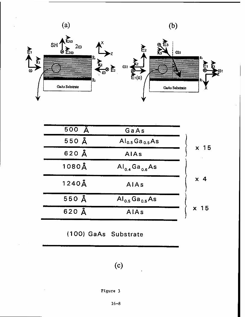
(a) (b)

500 A

550 A

620 A

1080A

1240A

550 A

620 A

GaAs

Alo.5Gao.5As

AlAs

A,o.4Gao.6As

AlAs

Al 0.5 G a 0.5 As

AlAs

x 15

x 4

x 15

(100) GaAs Substrate

(c)

Figure 3

16-8

TO-1 Transport

Optic

NJA-5 Modelocked Ti: Sapphire

Laser

Argon MNOVA-90 Laser

(a)

(b) Tr.Sapphire Laser Cavity

Figure 4

16-9

a. Saturation of photoluminescence peak

The PL spectra for several pump intensities are shown in Fig. 5. At laser intensity of

9.7 mW/cm2 there are two emission peaks: the one on the long wavelength side (-7780Ä)

corresponds to the emission of excitons at the interface islands while the other one (-7773Ä)

corresponds to the free excitons. When we change the laser intensity from 9.7 mW/cm2 to

1.4 W/cm2 at 4 K, we can see that the emission peak for the localized excitons loses its relative strength.

Due to growth interruption, a single PL peak breaks into two because of the formation

of interface islands with the size larger than the exciton radius. At low temperatures, all the

carriers generated by the pump laser will be eventually relaxed down to the lowest energy

levels and localized in the islands, resulting in large carrier densities. If the total area of the

islands is small, it would be possible to completely fill exciton states in these islands at rela-

tively low intensities, which manifests as the saturation of the PL peaks. This type of the

band-filling effect only occurs at the spatially-localized islands. The laser intensity required

to almost completely fill the localized exciton states is more than two orders of magnitude lower than that obtained before 113J.


We have made the time-resolved PL measurements in our sample. Fig. 6 shows the

typical temporal PL traces detected at the center wavelength of e1hh1 emission peak (the

excitonic emission peak) as a result of the carrier recombination at the interface islands. At

the low excitation intensity (207 W/cm2), the PL signal at the e,hh, (II) emission peak has a

decay time of about 269 ps. As the intensity increases, the decay time increases. As shown

in Fig. 6, when the laser intensity is 414, 621, and 828 W/cm2, the decay time is about 326, 537, and 666 ps.

In the quasi-CW regime, the density of excitons can be determined as

XT 'laser0

""laser

where Ilaser is the laser intensity, a is the absorption coefficient, and "hcolaSCT is the energy of a

single photon. The intensity required to completely fill the e,hh, exciton states is about

1.4W/cm2. Assuming a = 10000cm"1 at the pumping wavelength in our experiments, the

exciton density is then estimated to be 9.75x 1012cm~3. The corresponding area density is

1.46 x 10 cm-2. This carrier density is more than two orders of magnitude lower than that in Ref. [13].

16-10

oo

«w oo

o

££

o oo

U

u 00

16-11

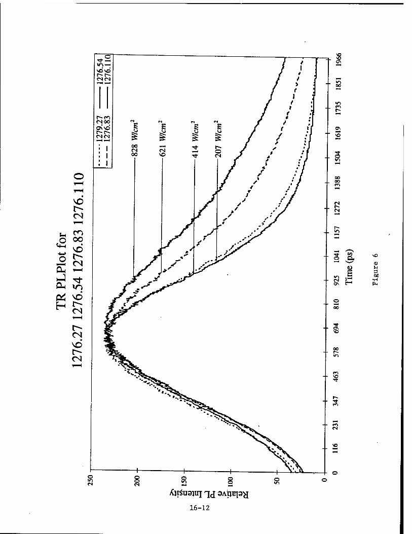
CO a,

1 93 U

M

16-12

c. Growth of a multilayer structure

Based on Refs. [11,12], we had already designed an optimized structure |see Fig. 3(c)].

We had grown this structure in collaboration with Drs. J. L. Loehr and J. Ehret at Wright

Labs. We will test the performance of this structure as an efficient frequency doubler and

optical parametric oscillator and amplifier at Bowling Green State University. The pump,

input and output wavelengths are designed to be 1.06 jim, 1.58 }im, and 3.23 (im. By chang-

ing the incident angle, one can tune the output wavelengths [12].

d. Attempt to mode-lock TirSapphire laser

The Ti:Sapphire laser is pumped by a re-furnished Argon laser (Coherent Innova 90),

see Fig. 4. For 4-watt pump power of a multi-line Argon laser, conversion efficiency as high

as 20% was achieved in CW regime. We had tried our best to mode-lock Ti:Sapphire laser.

We observed two-photon fluorescence in Coumarin 460, however, was not able to stablize

the mode-locked laser output. We believe that mode structure and pointing stability could be

the problems for mode-locking the TirSapphire laser. When there is no aperture for the

Argon laser, high-order modes other than TEM(H) exist in the Argon output beam profile. In

addition, we have crudely estimated the pointing stability as - 100|irad, which is an order of

magnitude larger than that required for stable mode-locking.

5. Conclusion

We have observed saturation of photoluminescence peak. We have measured time-

resolved photoluminescence decay in growth-interaipted asymmetric-coupled quantum wells.

We have subsequently determined decay times and characteristic carrier densities for the

observed photoluminescence intensity saturation. We have grown a multilayer structure that

can be used to implement an optical parametric oscillator and amplifier and frequency dou-

bler in a novel configuration. Finally, we have tried to mode-lock Ti:Sapphire laser and sum-

marized potential problems causing unstable mode-locked output.

Two journal papers based on our results will be submitted for publication.

6. Acknowledgement

We are indebted to Drs. J. P. Loehr, R. E. Sherriff, J. Ehret, J. Hoelscher, and D. C.

Reynolds for their expertise in the areas above, that had made it possible for us to work on

four different projects during ten-week period.

7. References

16-13

[1] D. Bimberg, D. Mars, J. N. Miller, R. Bauer, O. Oertel, and J. Christen, Supperlatt.

Microstruc. 3, 79 (1987).

[2] M. Kohl, D. Heitmann, S. Tarucha, K. Leo, and K. Ploog, Phys. Rev. B39, 7736 (1989).

[3] D. C. Reynolds, K. K. Bajaj, C. W. Litton, P. W. Yu, J. Singh, W. T. Masselink, R.

Fischer, and H. Morkoc, Appl. Phys. Lett. 46, 51 (1985).

[4] K. Fujiwara, K. Kanamoto, and N. Tsukada, Phys. Rev. B40, 9698 (1989).

[5] B. Devcaud, A. Chomctte, N. Roy, B. Scrmagc, and D. S. Katzer, Sur. Sei. 267, 199

(1992); D. Gammon, B. V. Shanabrook, and D. S. Katzer, Appl. Phys. Lett. 57, 2710

(1990).

[6] R. Normandin, R. L. Williams, and F. Chatenoud, Electr. Lett. 26, 2088 (1990); R. Nor-

mandin, H. Dai, S. Janz, A. Delage, J. Brown, and F. Chatenoud, Appl. Phys. Lett. 62,

118 (1993); D. Vakhshoori, R. J. Fischer, M. Hong, D. L. Sivco, G. J. Zydzik, G. N. S.

Chu, and A. Y. Cho, Appl. Phys. Lett. 59, 896 (1991).

[7] R. Lodenkamper, M. L. Bortz, M. M. Fejer, K. Bacher, and J. S. Harris, Jr., Opt. lett.

28, 1798 (1993).

[8] J. Khurgin, Appl. Phys. Lett. 21_, 2100 (1987): Phys. Rev. B38, 4056 (1988); J. Appl.

Phys. 64, 5026 (1988); J. Opt. Soc. Amer. B 6, 1673 (1989).

[9] S. Janz, F. Chatenoud, and R. Normandin, Opt. Lett. ]9, 622 (1994).

[10] J. B. Khurgin and Y. J. Ding, Opt. Lett. j9, 1066 (1994).

[11] Y. J. Ding, S. J. Lee, and J. B. Khurgin, J. Opt. Soc. Am. B ]2, 1586 (1995).

[12] Y. J. Ding, S. J. Lee, and J. B. Khurgin, Phys. Rev. Lett. 75, 429 (1995); Y. J. Ding, S.

J. Lee, and J. B. Khurgin, IEEE J. Quant. Electr. 3]_, 1648 (1995).

[13] A. G. Cui, Y. J. Ding, S. J. Lee, J. V. D. Veliadis, J. B. Khurgin, S. Li, D. C. Reynolds,

and J. Grata, J. Opt. Soc. Am. B J3, 536 (1996).

16-14

LASER BASED DIAGNOSTIC TECHNIQUES FOR COMBUSTION AND COMPRESSIBLE FLOWS

Gregory S. Elliott Assistant Professor

Department of Mechanical and Aerospace Engineering

Rutgers University P.O. Box 909

Piscataway, NJ 08855-0909


Wright-Patterson Air Force Base



and

Wright-Patterson Air Force Base

September 1996

17-1


Gregory S. Elliott Assistant Professor

Department of Mechanical and Aerospace Engineering Rutgers University

Abstract

Laser based diagnostic techniques were used and developed in the study of combustion and compressible flows. Laser diagnostic techniques based on using molecular filters to discriminate the Rayleigh scattering from molecules or particles in a flow field were investigated. The first technique termed filtered Rayleigh scattering was used to measure the instantaneous temperature field in hydrogen-air and methane-air flames. Uncertainties in these measurements were explored and found to be from 4 to 7% for the product region of the flame, but slightly higher (approximately 16%) in the reaction region of the flames studied. This uncertainty was primarily associated with the unknown species concentration and possible solutions to this problem will be investigated. A second molecular filter based technique called filter planar velocimetry (FPV) allows the measurement of the instantaneous velocity in a two dimensional plane. FPV was used to investigate axisymmetric and elliptic jets in a M = 2 cross flow. To date preliminary average measurements have been analyzed and are presented here. Lastly, flow visualizations were taken of underexpanded square jets to investigate the flow structure and use as a possible mixing enhancement configuration.

17-2


Gregory S. Elliott

I. THE USE OF FILTERED RAYLEIGH SCATTERING FOR PLANAR TEMPERATURE MEASUREMENTS IN COMBUSTION

LA. Introduction Techniques employing molecular filters to modify the light scattered from particles or

molecules in a flow offer the possibility of measuring single or multiple properties simultaneously.

The molecular filter is simply a cylindrical optical cell containing a molecule which has absorption

transitions within the frequency of the laser interrogating the flow field. The molecular filter is

placed in front of the receiving optics to modify the frequency spectrum of the scattering. Miles et

al.[1992] first demonstrated filtered Rayleigh scattering (FRS) employing molecular iodine filters

in conjunction with injection seeded, frequency-doubled Nd:YAG laser (A = 532 nm). With

injection seeding the linewidth is narrow (100 MHz) and the laser frequency can be tuned to match

the transitions of iodine. In addition to qualitative flow visualizations, Miles et al. [1992] showed

that average properties of the flow at each point in the illuminated plane can be obtained if the

scattered signal is collected from molecules. Recently Schrami et al. [1996] demonstrated that FRS

could also be used to obtain temperature measurements in lightly sooting flames, but there is still

a need for more comprehensive treatment of the uncertainties of the measurement technique.

LB. Experimental Arrangement Figure 1 gives a schematic of the burner and optical arrangement for the preliminary

measurements given here. Three different burners were used in this study. At Wright-Patterson Air

Force Base a hydrogen-air flame was studied using a Hencken burner with a 25 mm square

combustion region. The ability of FRS to record temperatures near the burner surface were

investigated in a methane/air flame created above a sintered bronze McKenna burner which is water

cooled to 283 K. The third burner is copper burner with an array of 64 1 mm diameter holes within

an area of 169 mm2. The interrogation laser beam was formed into a sheet with a combination of cylindrical and

spherical lenses. Two different frequency doubled Nd:YAG laser were used in the present

experiments a Spectra Physics GCR-150 (Henken and McKenen burner experiments at Wright

Paterson) with approximately 400 mJ per pulse and a Spectra Physics GCR-230 (copper burner

17-3

experiment at Rutgers) with 650 mJ per pulse. Both lasers have an injection seeder to provide a

narrow line width (~ 100 MHz) which can be tuned through the absorption lines of iodine around

532 nm. The Nd:YAG lasers used in these experiments have a pulse width of approximately 10 ns

with a repetition rate of 10 Hz. Two photodiodes were used to monitor the laser energy and

frequency fluctuations, using a second iodine filter. The Rayleigh scattering signal is collected using

a Princeton Instruments 14-bit intensified CCD camera. The images are stored on a Pentium 100

MHZ personal computer which provided camera control, laser synchronization, and frequency tuning control of the laser.

A major component of the FRS system is the iodine filter. The iodine filter is basically a

glass cylinder 9 cm in diameter and 24 cm in length with flat optical windows on both ends. Iodine

vapor is formed in the cell by inserting a small amount of iodine crystals and evacuating the cell.

The cell temperature (T^n) is raised above the ambient temperature with electrical heat tape so that

no iodine crystallizes on the windows. The coldest point in the cell is set in the side arm (Tn), which

is housed in a water jacket and maintained at a constant temperature by a circulation water bath. The

temperature of the side arm controls the vapor pressure (number density) of the iodine in the

absorption cell. The Nd: YAG laser has a narrow line width and at X = 532 nm it can be tuned across

the absorption bands of iodine. Figure 2 presents the absorption spectra with the two optically thick

absorption lines which were used in the present experiments at wave numbers of 18788.44 and

18789.28. The profile was taken with the cell operated at Tcell = 358 K and TI2 = 318 K.

I.C. Theoretical Description

Rayleigh scattering has been used to investigate combustion and flow fields for many years

and much of the theoretical analysis is well known. When interrogating a flow with a laser and

collecting the Rayleigh scattering signal from molecules, there are many important parameters

governing the scattered intensity (intensity of the illuminating light, polarization, frequency of the

illuminated light, etc.). In the current use of the FRS technique in combustion environments, the

intensity and spectral profile of the scattering are needed to deduce the temperature. Since the

flames studied here are at atmospheric pressure the Rayleigh scattering can be in the kinetic regime

and contain Brillouin scattering effects. Many different models exist for calculating the Rayleigh

scattering spectral profile [Yip and Nelkin, 1964 and Tenti et al.,1972] and have been confirmed by

experimental measurements [Lao et al., 1976]. The shape of the scattered spectrum is typically

parameterized by the dimensionless frequency X and the y parameter. The dimensionless frequency is nondimensionalized by the thermal broadening and is given by

X = s-2- . (1) 2sin(0/2) \j 2kT

17-4

where X is the wavelength of the incident light, (v -v0) is the frequency difference from line center,

0 is the angle between the incident and scattered wave vectors, k is the Boltzmann's constant, T is

the temperature of the gas, and M is the molecular mass. The y parameter (which is the ratio of the

collisional frequency to the acoustic spatial frequency) describes the shape of the Rayleigh scattering

spectrum and is given by

y = 4usin(6/2) \ 2kT

M (2)

where P is the pressure, and u is the viscosity. For y of the order of unity, the kinetic regime,

Brillouin components become important and kinetic models must be used. For y «1 (low pressures

or high temperatures) the scattering spectrum is Gaussian and the Brillouin components can be

neglected. The total spectral intensity is given by the intensity of the scattering of the ith gas species

weighted with its mole fraction x; and Rayleigh cross section oRi and is given by

I(v) =CI0N^. xioRir.(T,P,M.,e,v) (3)

where C is the optical calibration constant, I0 is the incident laser light intensity, N is the total

number density, and r, is the scattering distribution of the ith gas species determined by the kinetic

model (ie. S6 model used by Tenti et al., 1972). The intensity collected by the camera is a convolution of the total spectral intensity [I(v )]and

the transmission profile [A(v)] as shown schematically in Figure 3. As illustrated in Figure 3 the

scattering from particles and surfaces has a narrow linewidth and is attenuated by the iodine filter.

Since the Rayleigh scattering from molecules is thermally broadened much of the scattered intensity

passes outside the absorption profile (as illustrated by the shaded region of Figure 3). This is a

significant characteristic of FRS since molecular Rayleigh scattering is weak relative to surface and

particle scattering. In order to eliminate the dependence on the optical calibration constant and on the incident

laser irradiance distribution, images with the flame on were normalized by scattering collected from

the air at ambient conditions. For the present experiments only premixed flames are considered and

the dominate species is nitrogen, and therefore the scattering will be assumed to be from a single

species. Also the velocity component with the current arrangement leads to little change in

frequency due to Doppler shift and so it will be ignored in the present analysis. With these

assumptions and since the flames are all at atmospheric pressure the intensity is a function only of

temperature for a given optical arrangement and the ratio is given by

17-5

S(V) _ NNjqN/(T»P.MN2»e>V)A(V~V/)dV' S-(V) Nair]

,aa.rr(TSTp,PSTp,Mair,05v)A(v-v/)dv/ (4)

The local gas temperature influences the collected intensity through the gas number density (N) and

the thermal broadening which increases the portion of the scattering which is not absorbed by the

filter. Thus if the normalized intensity ratio is known [S(v)/Sair(v)] the temperature can be determined.

I.D. Hydrogen-Air Flame Results

Figure 4 gives the two dimensional temperature field (x-y view) for a hydrogen-air flame ($

= 0.25) 2 cm above the Henken burner with a plot of the temperature profile in the center of the

image given below the appropriate image. It should be noted that no particular care was taken to

physically eliminate particles in the flame or in the surroundings. Scattering from particles generally

will dominate the Rayleigh scattering, however, in the present experiment the particle scattering is

strongly absorbed since it is not thermally broadened. The adiabatic flame temperature in this case

is 1065 K. The first case (Fig. 4a) shows a single shot instantaneous temperature field with the

average temperature away from the edges of the flame being 1062 K. The instantaneous temperature

profile has a high degree of fluctuation in what should be a relatively flat profile as shown by CARS

measurements. Most likely this fluctuation is due to the photon statistics. Thus the signal to noise

ratio can be improved by either increasing the number of photons collected (more laser energy per

pulse), low pass filtering, or binning multiple pixels together. Figure 4b shows the effect of binning

3 adjacent pixels together (Fig. 4c) and as expected the random temperature fluctuations decrease,

but at the cost of decreased spatial resolution (from 0.1 mm2 to 1 mrrr ). Figure 4c is the two-

dimensional temperature field made by averaging 40 instantaneous images together. As expected

this shows the least amount of temperature fluctuation, but of course the instantaneous information is lost.

Figure 5a and 5b give the average temperature and standard deviation of the temperature in

the flat portion of the hydrogen-air flame for various equivalence ratios. The temperatures measured

with FRS are in excellent agreement with the adiabatic flame temperature. The maximum deviation

is at the highest temperatures with the FRS measurements always slightly lower as expected. The

standard deviation of the temperature across the flat portion of the flame is given in Figure 5b for

the instantaneous, bin by 3, and average temperature fields for various equivalence ratios. As

expected binning the pixels of the instantaneous image by three increases the signal to noise ratio

by approximately three for all cases which would be the case if the fluctuations were a result of

17-6

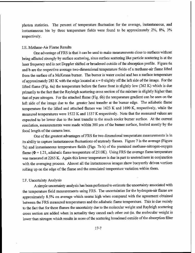
photon statistics. The percent of temperature fluctuation for the average, instantaneous, and

instantaneous bin by three temperature fields were found to be approximately 2%, 8%, 3%

respectively.

I.E. Methane-Air Flame Results One advantage of FRS is that it can be used to make measurements close to surfaces without

being affected strongly by surface scattering, since surface scattering like particle scattering is at the

laser frequency and is not Doppler shifted or broadened outside of the absorption profile. Figure 6a

and b are the respective average two-dimensional temperature fields of a methane-air flame lifted

from the surface of a McKenna burner. The burner is water cooled and has a surface temperature

of approximately 283 K with the edge located at x = 0 slightly off the left side of the image. For the

lifted flame (Fig. 6a) the temperature before the flame front is slightly low (262 K) which is due

primarily to the fact that the Rayleigh scattering cross section of the mixture is slightly higher than

that of pure nitrogen. For the attached flame (Fig. 6b) the temperature gradient can be seen on the

left side of the image due to the greater heat transfer at the burner edge. The adiabatic flame

temperature for the lifted and attached flames was 1623 K and 1690 K, respectively, while the

measured temperatures were 1522 K and 1537 K respectively. Note that the measured values are

expected to be lower due to the heat transfer to the much cooler burner surface. At the current

resolution, measurements were made within 300 urn of the burner surface, limited mostly by the

focal length of the camera lens. One of the greatest advantages of FRS for two dimensional temperature measurements is in

its ability to capture instantaneous fluctuations of unsteady flames. Figure 7 is the average (Figure

7a) and instantaneous temperature fields (Figs. 7b-h) of the premixed methane-nitrogen-oxygen

flame ($ = 1.21, adiabatic flame temperature of 251 OK). Using FRS the average flame temperature

was measured at 2265 K. Again this lower temperature is due in part to unsteadiness in conjunction

with the averaging process. Almost all the instantaneous images show buoyantly driven vortices

rolling up on the edge of the flame and the associated temperature variation within them.

I.F. Uncertainty Analysis A simple uncertainty analysis has been performed to estimate the uncertainty associated with

the temperature field measurements using FRS. The uncertainties for the hydrogen-air flame are

approximately 8.5% on average which seems high when compared with the agreement obtained

between the FRS measured temperatures and the adiabatic flame temperature. This is due mainly

to the fact that for these flames the uncertainty due to the molecular weight and Rayleigh scattering

cross section are added when in actuality they cancel each other out (ie. the molecular weight is

lower than nitrogen which results in more of the scattering broadened outside of the absorption filter

17-7

and the Rayleigh scattering cross section is lower than nitrogen resulting in less signal). Taking this

fact into consideration reduces the uncertainty to approximately 5% which is more in line with the measurements.

The highest uncertainties (above 10%) were found to be within the reactant region of the

methane flame particularly for the flame with the equivalence ratio of 1.2. The predominance of

methane with a Rayleigh scattering cross section twice that of nitrogen causes the temperatures to

be under estimated as is seen in the FRS measurements presented in Figure 6 and 7. The product

region of the flame, however, shows a lower uncertainty of approximately 4% for these methane

flames since the molecular weight and Rayleigh scattering cross section is much closer to nitrogen.

The uncertainties for the instantaneous images are higher (due to higher noise in the recorded

intensity) being approximately 20% for the reactant region and 7% for the product region of the

flame. It should also be noted here that the values for the uncertainty of the independent variables

were generally over estimated resulting in very conservative estimates of the total uncertainty in the

temperature measured with FRS.

II. FILTER PLANAR VELOCIMETRY MEASUREMENTS OF A JET IN A M = 2 CROSS FLOW

ILA. Introduction

Although filtered Rayleigh scattering relies on scattering from molecules for the temperature

measurements described above, other techniques use scattering off of particles natural present or

seeded into the flow. These molecular filter Based velocity techniques have been developed to

measure the average velocity (Doppler Global Velocimetry, DGV, [Meyers and Komine, 1991]) or

instantaneous velocity (Filtered Planar Velocimetry, FPV, [Elliott et al., 1994]). FPV utilizes two

cameras. One camera has a pressure broadened iodine filter in front of it which produces gradual

slopes (Figure 8) in the absorption profile instead of the sharp temperature broadened filter used by

Miles et al. [1992]. A second camera with no filter (similar to DGV) is used to normalize the image

from the filtered camera, accounting for variations in laser intensity, and particle size and density

in the measurements. When the laser frequency is tuned to the edge of the sloping region, the

Doppler shift will move the scattered intensity into the sloping region of the absorption profile

resulting in a deviation in the transmission ratio (Figure 8). The Doppler shift is given by

AfD = {(L~kJ-z (5)

where k, and k0 are the observed and incident unit light wave vectors, respectively, and V is the flow

17-8

velocity vector. Thus when the transmission ratio is calculated from the two cameras the frequency

shift can be obtained and the velocity is calculated from Equation 6. Instantaneous velocities have

been measured in compressible mixing layers [Elliott et al., 1994] and multiple velocity components

in boundary layers [Arnette et al., 1995] using FPV.

II.B. Experimental Arrangement

The flow field studied using FPV was a jet in a Mach 2 cross flow which utilized the

supersonic research facility at Wright-Paterson Air Force Base. Details of this facility are presented

elsewhere [Gruber et al. 1996]. Figure 9 gives a schematic of the tunnel, laser, and camera geomtry.

The test section for these experiments has a constant area test section with a cross section of 131mm

by 152 mm. The tunnel can be run continuously with a stagnation temperature and pressure of 300

K and 317 kPa respectively resulting in an average free stream velocity of 516 m/s. Two different

injector geometries, circular (6.35 mm diameter) and elliptic (6.2 mm major axis and 1.63 minor

axis, effective diameter of 6.35 mm) were incorporated into removable test inserts housed within the

bottom wall of the test section. The exit pressures of both jets were regulated to 476 kPa resulting

in a jet to free stream momentum flux ratio of 2.93. Particles were seeded into the freestream by the

combustion of silane which produces silicone dioxide particles in the range of 0.2 [am diameter.

The laser and camera system used here was the same as in the FRS experiments with the

exception of an additional camera which recorded the normalized image for each instantaneous

filtered image. Another difference between the FRS and FPV system is in the absorption properties

of the iodine filters used with each system. Figure 10 shows the difference between the two filter

profiles used in this study. The filter profile used in the FRS measurements was dominated by

thermal broadening resulting in relatively sharp slopes on either side of the profile. The absorption

profile used for FPV has a much more gradual profile which is made by introducing a nonabsorbing

gas (nitrogen with a partial pressure of 15 torr) into the iodine filter. This results in the absorption

profile being dominated by pressure broadening effects which can be used to adjust the slope for the

expected frequency range encountered in the flow studied.

In the past when making velocity measurements using molecular filter based techniques a

problem is encountered in measuring a velocity component which is "natural" to the flow being

studied is difficult without using more than one camera pair or viewing the flow at oblique angles.

To circumvent this problem we chose to use the laser optical arrangement of Figure 9 and reflect the

laser sheet back on itself. From Equation 6 it can be shown that for the present arrangement this

results in a sensitivity to the velocity vector essentially in the streamwise direction and instantaneous

streamwise velocities can be obtained. In order to find information about the spanwise velocity a

single laser pass was used resulting in a velocity vector 40 degrees from the streamwise direction.

Although the spanwise velocity component can not be decoupled from the streamwise velocity

17-9

component for the instantaneous measurements, for the average velocity field both optical

arrangements can be combined to calculate the spanwise velocity component.

II.C. Preliminary results

Measurements were taken at several streamwise locations for the circular and elliptic jet

injection geometries both with and without the laser sheet reflecting back on itself. At the present

time only the average velocity images have been reduced. Figure 11 gives of the unfiltered image

and streamwise velocity image for the circular jet, and the spanwise velocity image for the elliptic

jet. For these preliminary results the freestream velocity was used to calibrate the measurements

which will not be necessary when the instantaneous images are fully analyzed. As expected the

streamwise velocity image shows the velocity decrease after the bow shock consistent with the shock

angle which the flow has passed through. The streamwise velocity decreases further as the jet core

and boundary layer are approached. It should be kept in mind, however, that the jet was not seeded

and therefore the measurements in the core region are biased by the free stream velocity resulting

in a higher value than is really the case. The spanwise velocity image shows essentially zero

spanwise velocity outside the bow shock and in the core of the jet. There are however positive and

negative spanwise velocity components inside the bow shock to the left and right of the jet

respectively. This is most likely due to the streamwise vortices which are formed around the jet.

It should be emphasized that these results are very preliminary and further conclusions will be drawn

as the instantaneous images are calculated.

III. FLOW VISUALIZATIONS OF AN UNDEREXPANDED SQUARE JET

III.A. Introduction

In recent years much effort has been devoted into investigating non-circular (ie. square,

rectangular, elliptical) jets and the possibilities of their use to enhance mixing particularly in the

compressible flow regime [Grinstein, 1996 and Glawe, 1995]. These non-circular geometries find

applications in thrust vectoring, enhancing entrainment for combustion, and heat signature reduction.

Square jets have shown 45 degrees of axis rotation in the near field caused by the vortex dynamics

in the corners of the jet. Although these observations have been made there is still a need to better

understand the fluid mechanisms which govern these observations. As a first step toward this goal,

flow visualizations and FPV images have been taken in an under expanded square jet. Preliminary

images are given here with the majority of the data still to be processed.

17-10

III. B. Experimental Arrangement

The laser and camera system were the same as described previously for the FRS and FPV

experiments, allowing instantaneous (pulse width of 10 ns) images to be taken. The square jet

studied has a 25.4mm by 24.5mm cross section and can be operated continuously with the supply

air at the Wright-Patterson Air Force Base supersonic research facility. Stagnation pressures from

240 to 517 kPa were studied which resulted in an underexpanded jet for all conditions. Two

different laser sheet orientations were investigated one aligned parallel to the jet axis (streamwise

view) and one with the sheet aligned perpendicular to the jet axis (spanwise view). The scattering

was collected from ice particles formed from the moisture in the supply air as the temperature

decreases through the nozzle (marking the core of the jet), and as the moist ambient air mixes with

the colder supersonic air (marking the mixing region of the jet). These ice particles have been used

by other investigators to study various flow fields using similar techniques [Elliott et al., 1992].

III. C. Preliminary Results and Discussion Average streamwise images are given in Figure 12 for the square jet operated at P0 = 240 to

517 kPa. Each average image is calculated from 120 instantaneous images and normalized to

remove the Gaussian intensity distribution in the laser sheet. Oblique shock and expansion waves

are clearly visible above a stagnation pressure of 310 kPa. What appears to be a Mach disk occurs

for stagnation pressures above 380 kPa at an x/s ~ 1.5 (where s is the height of the jet).

Instantaneous streamwise images are given in Figure 13. For P0 = 240 and 345 kPa large scale

structures are apparent with alternate spacing above and below the jet centerline similar to what is

seen in axisymmetric jets when a helical mode is present. Also the instantaneous shock/expansion

wave pattern is much different than the average images for the P0 = 345 kPa case. Spanwise images

were taken for each operating pressure at various downstream locations. Average spanwise images

for the square jet operating at P0 = 276 and 517 kPa are given in Figure 14. For the lower stagnation

pressure case evidence of streamwise vorticity in the corners of the jet is visible, but there appears

to be no axis rotation as the shear layers on the sides of the jet develop down stream. For the higher

stagnation pressure case (P0 = 517 kPa), however, axis rotation of 45 degrees is observed as the

complex shock and expansion wave patterns develop downstream.

IV. ACKNOWLEDGMENT I would like to acknowledge Dr. C. Carter, Mr. J. Donbar, Dr. D. Glawe, Dr. M. Gruber, and

Dr. A. Nejad for running these experiments (sometimes late at night) and building the facility to

allow the research to take place. Also, I would like to acknowledge the support of AFOSR for

funding this work and the National Science Foundation for providing funding for part of the

equipment used here under grant number NSF-9622108 with Dr. R. Arndt.

17-11

IV. REFERENCES

Arnette, S.A., Samimy, M., and Elliott, G.S., "Two-Component filtered Planar Velocimetry

in the Compressible Turbulent Boundary Layer" Submitted to the AIAA 34th Aerospace Sciences Meeting, 1996.

Elliott, G.S., Samimy, M., and Arnette, S.A., "Study of Compressible Mixing Layers Using

Filtered Rayleigh Scattering Based Visualizations," AIAA Journal, Vol. 30, No. 10,1992.

Elliott, G.S., Samimy, M., and Arnette, S.A., "A Molecular Filter Based Velocimetry

Technique for High Speed Flows," Experiments in Fluids, Vol. 18, pp. 107-118,1994.

Glawe, D.D. "Parallel Injection from the Base of an extended Strut Into Supersonic Flow,"

Ph.D. Dissertation, The Ohio State University, 1995.

Grinstein, F.F. "Dynamics of Coherent Structures and Transition to Turbulence in Free Jets,"

AIAA Paper 96-0781,1996.

Gruber M.R., Nejad, A.S., Chen, T.H., and Dutton, J.C., "Large Structure Convection

Velocity Measurements in Compressible Transverse Injection Flowfields," AIAA Paper 96-0203, 1996.

Lao, Q.H. Schoen, P.E., and Chu, B., "Rayleigh-Brillouin Scattering of Gases with Internal

Relaxation," The Journal of Chemical Physics, Vol. 64. No. 9, pp. 3547-3555, 1976.

Meyers, J.F., and Komine, H., "Doppler Global Velocimetry: A New Way to Look at

Velocity," Laser Anemometry, Vol. 1,1991.

Miles, R.B., Forkey, J.N., and Lempert, W.R., "Filtered Rayleigh Scattering Measurements

in Supersonic/Hypersonic Facilities," AIAA Paper 92-3894,1992.

Schrami, S., Will, S., Hofmann, D. Munch, K.U., and Leipertz, A., "Two-Dimensional Laser

Diagnostics for Sooting Flames," 8th International Symposium on Applications of Laser Techniques to Fluid Mechanics, 1996.

Tenti, G, Boley C, and Desai, R., "On the Kinetic Model Description of Rayleigh-Brillouin

Scattering from Molecular Gases," Canadian Journal of Physics, Vol. 52, pp. 285-290, 1974.

Yip, S. and Nelkin, M., "Application of a Kinetic Model to Time-Dependent Density

Correlations in Fluids," Physical Review, Vol. 135, 1964, pp. A1241-A1245.

17-12

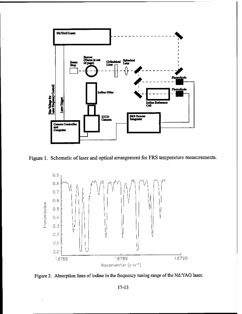
N&YfcQLMcr

CyHndrkal ffijf*1

Photodiode

S.-E3 PhctodJooc

Cefl

SRS Boxcar

Figure 1. Schematic of laser and optical arrangement for FRS temperature measurements.

c o

'a) CD

c o

18788 18789

Wavenumber (cm-1)

18790

Figure 2. Absorption lines of iodine in the frequency tuning range of the Nd:YAG laser.

17-13

Background Scattering from Surfaces and Particles

Absorption Filter Profile

Rayleigh Scattering Spectral Profile

5 6 7 8 9

Frequency

Figure 3. Schematic of absorption profile convoluted with molecular Rayleigh scattering.

a)

c)

b)

-ISO -100

MOO

1200

1000

800

600

400

300

-150 -100 SO 0 50 100 150 Rndius (mm)

1250

Li looo

"750

500

■250K

Figure 4. Instantaneous (a) bin by 3 (b) and average (c) images and temperature profiles taken using FRS above a hydrogen-air flame.

17-14

a)

e

b)

2500

2300 2100

1900

1700

1500

1300 1100

900 700

500

300

100

200

ISO

160

140

120

100

80

60

40

20

0

0.0 0.1 0.2 0.3 0.4 0.5 0.6 0.7 0.8 0.9 1.0

Equiv. Ratio

"

A--'

A...-

>"''""' " -■-'A

- - ~ A--- Instantaneous

-

^..'i

si.

X _.——-*— _—-"■

*•' S--^ll_»—-•——

■.-- _..---■"""""" ,-—■

- i i , i . , . , .

0.0 0.1 0.2 0.3 0.4 0.5 0.6 0.7 0.8 0.9 1.0 Eqiv. Ratio

Figure 5. Average temperature (a) and standard deviation (b) of the temperatures for a hydrogen- air flame operated at various equivalence ratios.

a)

10 mm 20 30 40 50 60 70 80

b)

2000

! 1500

1000

500

250 K

10 mm 20 30 40 50 60 70 80

Figure 6. Average two-dimensional temperature fields of a methane-air flame lifted (a) and attached (b) to the burner surface.

17-15

o o

© o o cs

o o

o o o

o ©

CO

CO

a •a es

s

CD l-i OH

CS <L> CO

O CO

iß u

CS

u

u co 3 O CD

i co C

§ CD

CS0

l-H CD >

CD

3 bp

17-16

Unshifted Background Light

Absorption Profile

Doppler Shifted Scattering

[o Frequency

Figure 8. Schematic illustrating Filtered Planar Velocimetry.

Minor

^7-^Y

~^

Nd:YAG Laser

Sperical Lens

1 Cylindrical Lens ^^

DZZZZ

<>Jet Flow Direction

Cylindrical Lens

Mirror

Iodine Filter

Window EZZZZZ

ICCD Camera

Figure 9. Plan view of the tunnel and optical arrangement for FPV measurements of a jet in a supersonic cross flow.

17-17

1.1

1.0

0.9

0.8

0.7

0.6

0.5

0.4

0.3

0.2

0.1

0.0

2 3

Frequency(GHz)

Figure 10. Iodine absorption filter profiles with and without pressure broadening from nitrogen.

a)

75 m/s

-75 m/s

Figure 11. Reference (a), streamwise velocity (b), and spanwise velocity (c) average images of a jet in a Mach 2 cross flow taken using FPV.

17-18

Figure 12. Average streamwise flow visualizations of underexpanded square jets operated at stagnation pressures (kPa) of 240 (a), 276 (b), 310 (c), 345 (d), 380 kPa (e), 414 (f), 450 (g), and 517(h).

17-19

Figure 13. Instantaneous streamwise flow visualizations of underexpanded square jets operated at stagnation pressures (kPa) of 276 (a), 345 (b), 414 (c), and 517 (d).

x/s = 0.5 x/s=l x/s = 2 x/s = 3

Figure 14. Average sspanwise flow visualizations of underexpanded square jets operated at stagnation pressures (kPa) of 276 (a-d), and 517 (e-h).

17-20

VERTICAL 3-D INTERCONNECTS FOR

MULTICHIP MODULES

Altan M. Ferendeci

Associate Professor


and Computer Science Department


Rhodes Hall 823, ML-30

Cincinnati, Ohio 45221-0030

Final Report for:


Wright Laboratories

Sponsored by

Air Force Office of Scientific Research


and

Wright Laboratory

August 1996

18-1


MULTICHIP MODULES

Altan M. Ferendeci

Associate Professor


and Computer Science Department


Abstract

In this report, a vertically-connected 3D T/R module for a conformal phased array antenna

systems is investigated. Active and passive elements and circuits suitable for the proposed 3/D

modules are analyzed. The module involves the use of thermally shunted HBT for power

amplifier, various distributed circuit elements realized by coplanar waveguides (CPW), and vertical

posts interconnecting the various circuit layers. Coplanar waveguides completely immersed in a

dielectric medium and surrounded by an upper and a lower ground plane is analyzed using

conformal mapping. It is shown that if the separation distance between the side ground planes of

the CPW is small compared to the vertical distances to the upper and lower ground planes, the

impedance of the line becomes independent of the dielectric layer thickness. Sycar is chosen as the

dielectric material. Uniformity and thickness control during the processing of sycar will lead to

reliable low loss vertical interconnects. The goal of the project is to implement a 3D T/R module

and demonstrate the feasibility of 3D vertical interconnects by incorporating these modules in a 2x2

phased array antenna system.

18-3


MULTICHIP MODULES

Altan M. Ferendeci

Introduction

At present, solid state power sources can not replace the high power slow-wave microwave

tubes. But by incorporating novel power combining techniques, the overall combined power of the

solid state sources may approach that of a single tube output. This is especially true for phased

array antenna systems where each radiator has its own power amplifier and the total radiated power

is the combined power of all the radiators. In a phased array antenna system, the transmit/receive

(T/R) modules are placed on a line (linear array), on a plane (planar array) or on a circular area

(circular array). To eliminate the main side lobes, the separation distance between the antennas

should be less than half the free space wavelength of the radiated signal.

At microwave and millimeter wave frequencies, planar antennas are replacing the

conventional antenna structures. The dimensions of the patch antennas are generally less than the

required free space half-wavelength. They can be configured to be used in any array configuration.

Unfortunately, if a compact module including all the electronics is to be integrated with the patch

antenna, it is impossible to place all the individual circuit modules on the same substrate and at the

same time satisfy the antenna spacing requirements. This becomes more important especially at

millimeter wavelengths. Even though most of the system components are in the form of monolithic

integrated circuits, they still occupy a large surface area of a substrate. Even if the complete circuit

can be laid out on the same GaAs or InP substrate, it will too expensive to use this type of large

area substrates behind each of the radiator . The complete transmit/receive (T/R) module also

contains a high power amplifier. Unless precautions are taken to remove the generated heat,

placing this circuit on the same substrate with other temperature sensitive circuits such as low noise

preamplifiers may not be desirable. Even if lumped elements are replaced by distributed elements at

higher frequencies, the overall T/R module may still require a large substrate area.

At present, all circuit modules are placed an enclosed casing. The power is coupled to the

antenna through one end of the casing. Unfortunately, this increases the overall depth of the T/R

module relative to the lateral dimensions of the antenna. These modular units have the distinct

disadvantage of having a surface area to depth ratio very small. Even with these limitations, they

can still be utilized in a linear or a planar array. They can not be distributed over a general curved

surface. For a module to be universally conformal to any surface, the depth of the module should

be negligibly small compared to the maximum lateral dimensions of the modular unit.

18-4

It is possible to place the circuit modules vertically one over the other so that the final T/R

module will occupy less space. 3D module configuration dictates the development of a new

packaging technology so that various circuit modules at various levels can be vertically

interconnected with each other with little or no loss in signal amplitude, with no cross coupling

between the elements and with manageable processing steps.

There is already considerable research and development effort being extended to

incorporate vertical interconnects in the implementation of monolithic microwave integrated circuits

(MMIC)[1,2]. There are two major concentrated research areas that utilize 3D vertical

interconnects. First area is the use of vertical interconnects for compacting the size of an integrated

circuit module [3]. In this scheme, thin multiple dielectric layers (2.5 ^im) are used for connecting

the various elements of the circuit together. The second major concentrated effort is to stack

various circuit modules of the overall T/R module one over the other using vertical interconnects.

Actually both of these concepts complement each other since the final T/R module may contain

various vertically interconnected MMICs.

In either case, coupling of microwave or millimeter wave signals between the layers

become a major area of research. Already, there is considerable research work going on related to

the coupling mechanisms between transmission lines of the various layers [4]. Novel transmission

lines are also proposed and analyzed [5-9].

In this report, a complete 3D vertically interconnected 3D T/R module for a conformal

phased array antenna system is proposed. Details of the proposed configuration including an

integral patch antennas will be given. The major components of the T/R module and the specific

areas that have to be developed will be discussed.

Phased Array Antenna Module

Typical front end of a T/R module for a radar system is shown Figure 1. Figure 2 shows a

2x2 modular phased array antenna system. The control and processing electronics are not shown in

these figures. The lowest substrate layer contains the power amplifier. Heat can be easily

transferred from the substrate by placing the overall module on a highly heat conducting metallic

surface.

Various layers of the T/R module are processed by deposition of multiple dielectric

materials of known thickness followed by metal depositions immersed between the dielectric

layers. As the module is processed, necessary interconnecting posts (or vias) are electro-deposited

and the circuit for that layer is finally processed.

18-5

The upper layer of the module has a patch antenna which could be either in rectangular,

circular or ring shape [10]. The thickness of the upper dielectric layer below the patch can be

adjusted to provide the maximum radiation condition for a specific antenna [11].

Typical dimensions for patch antennas operating at 10 GHz and with a dielectric material of

£=2.5 are given in Table I. The overall dimensions of these patches are smaller than Xfi.=15 mm

and thus can be used in phased array antenna systems since they easily satisfy the phased array

antenna spacing requirements.

Power TR Phase Amplifier Switch Shifter

/ \ / \ A. I \ /IF Afarxi.x V \ A \

V \ \

Patch

Control

«— ^Ui™ ~—=^- -»- ■'! ■ * ■*-f ■ B' HW -—< ■ ■« BIX ■*"! 1 Ml <: *-* ■

Substrate K ■ ft t

Figure 1. Major components of a T/R module.

Figure 3 shows possible distribution of vertically interconnected 3D T/R modules over

various surface configurations. These surface can actually be of any shape provided the radius of

curvature of the surface is not too small compared the lateral dimensions of the T/R module. Since

the overall thickness of the proposed vertically interconnected 3D T/R module is expected to be a

few millimeters, they can easily be distributed over any conformal surface topology. These

properties may lead to vast number of applications in communication and radar systems.

18-6

Table I. Dimensions of a patch antennas

(f=10GHz, X/2 = 15mm, e=2.5)

Patch Dimensions (mm) Directivity (dB)

Rectangular w=11.3, L=10.8 6.9

Circular D = 10.8 7.1

Ring b=4.1, a=2.6 <7.0

Modules

Figure 2. 4 element phased array antenna system with 3D T/R modules.

Figure 4 shows the essential components of a typical representative vertically

interconnected 3D T/R module. A substrate (preferably a Si-Silicon or Alumina) is the base of the

building block. Since the substrate can be attached to another heat conducting material such as a

metal, the power amplifier circuitry is processed on this substrate. The power amplifier chip is

attached to the Si-substrate by micromachining an opening on the Silicon surface and flip bonding

18-7

of the chip into the opening [12,13]. Since the dielectric thickness of the vertical layers are

relatively thin and their thickness may be comparable to the overall height of a thermally shunted

HBT, it is recommended that the micromachining depth should be as deep as the transistor height

so that the ensuing dielectric layers can be deposited uniformly over the substrate material.

Planar

##i%®:;#j%# y^AAAJUT

Figure 3. Distribution of patch antennas over a line, plane or a cylinder.

Circuit plane

Gnd Plane

Circuit plane

Gnd Plane

Vertical Interconnects

Transmission Power Lines Amplifier

Figure 4. Representative components of a 3D module.

18-8

There are four major areas that have to be developed in implementing a vertically

interconnected 3D T/R module. These are:

a) Power amplifier

b) Transmission lines and passive circuit components

c) Deposition and processing of dielectric layers

d) Low loss vertical interconnects.

Power Amplifier.

There are many possibilities for the implementation of the power amplifier. The complete

power amplifier can be processed as a monolithic integrated circuit using either HBTs or FETs,

Since there is a very successful development program on thermally shunted HBT power devices

(Figure 5) at the Devices Branch of the Electronics Division of the Avionics Laboratory (AADD) of

the Wright Laboratory [14], it will be an excellent opportunity to incorporate these devices in the

proposed 3D T/R modules. This will also allow close collaboration between the various branches

of the Electronics Division. The combined expertise of the various branches will lead to the

development of the best circuit topology for maximum operational efficiency.

Thermal Shunt

Emitter Fingers"

Figure 5. Thermally shunted power HBT developed at AADD of Avionics

Laboratory (Ref. 14).

Transmission Lines

There are many transmission line configurations that can be used in the implementation of

the vertically interconnected 3D T/R modules [15,16]. Microstrip lines, strip lines, slot lines and

coplanar waveguides are the best possible candidates that can be used with these modules. Because

of the unsymmetric nature of the slot line, it has limited applicability and in general is used for line

18-9

couplings between various layers. In many cases, circuit planes will be sandwiched between two

conducting ground planes. Therefore microstrip lines are replaced by stripline type transmission

lines. If the upper dielectric layer of a circuit plane is relatively thick compared to the lower

dielectric layer, microstrip like transmission lines can still be implemented with a slight

modification to the line characteristic. In this case, the strip is now embedded completely in a

dielectric material of 8r.

(a)

V' Photo-resist

Silicon

Metal Deposition

Etch #1 (b)

(c)

Etch #2 (d)

\^ / Low melting point

Thermal SI-GaAs Shunt Substrate

Gold Electrode HBT

Meta

4r

Si Substrate

Conductor

^-^

Dielectric

Si Substrate

Figure 6.3 Micromachining steps in Silicon for attaching the HBT chip. The transistor shunt metal

makes direct contact with Si-substrate.

(a) Stripline (b) Coupled Striplines

(c) Coplanar Waveguide (d) Coupled Coplanar Waveguide

Figure 7. Transmission line suitable for 3D interconnects.

18-10

In selecting transmission line structures best suited for the proposed 3D T/R module, the

lines should have low loss, easy to process and above of all they should be less sensitive to the

thickness of the processed dielectric layers. If the thickness of the dielectric layer can be controlled

accurately, the choice of the transmission line structure will not be critical.

For a circuit plane sandwiched between two ground planes, striplines (SL) and coplanar

waveguides (CPW) are the two best transmission line configurations that can be used in

implementing the passive elements of a vertically interconnected 3D module.

Figure 7 shows the stripline and the coplanar waveguide in the presence of both upper and

lower conducting planes. If the upper conducting ground plane is not present, the stripline

becomes a modified microstrip transmission lines imbedded in a dielectric material. Already

successful power coupling configurations from one layer to the other are implemented when the

lines are embedded within multiple dielectric layers [2].

X1

i x-plane

h1 -b >;sr ::-iä:: b

h2 V X3 *4 ;?•■

*;

(a)

z-plane (b)

w, w w-plane

w w lw w 4 5l 6 1

(C)

Figure 8. Conformal mapping of the CPW with top and bottom

ground planes immersed completely in a dielectric material.

18-11

In order to verify the suitability of CPW for the proposed 3D modules, the effect of the

upper and lower ground planes on the impedance characteristic of the coplanar waveguide is

investigated. The geometry given in Figure 8a represents a typical coplanar waveguide imbedded in

a dielectric material sandwiched between two conducting planes separated by distances h, and h2.

A quasi-electrostatic solution for the CPW can be found by using conformal transformations [17-

19]. The geometry given in Figure 8.a is treated as two separate problems, one for the upper and

one for lower parts of the transmission line. Both parts can be transformed into the z-plane through

the transformation

TEC z- tanh(—)

2Ä

The transformed z-plane coordinates are shown in Figure 8b. The z-plane is then

transformed into the w-plane using elliptic transformations (Figure 8c). The resulting characteristic

impedance can be written as

z<= 60 n — Kikl—mj-(Q) w 'eff Kw\) K(k\y

Here

k3 = tanh(^a/2/i1)/tanh(^/2/z])

k2 = tanh(^a/2/?2)/tanh(^/2Ä2)

and K(k) is the Complete Elliptic Integral of the First Kind with argument k and k' = V1 - k2.

Since the whole line is imbedded in a dielectric material, the £eff=er.

A FORTRAN program is written and the thickness of the dielectric layers between the

upper and lower ground planes are taken to be equal. For a gap of 2 |im and width of 20 (im, the

variation of the line impedance as a function of the dielectric thickness h is plotted as shown in

Figure 9. The impedance is not effected as the dielectric thickness becomes greater than twice the

overall separation distance of the two side ground planes. Therefore, for dielectric layer thickness

grater than 2(W+2S), the CPW parameters will not be critically dependent on the small differences

in the thickness of the deposited dielectric layers.

18-12

M P E D A N C E

50.0 A

/

/

24 48 72

HEIGHT (pm)

96 120

( W=20 um,G=2]Jim h=50um)

Figure 9. Impedance variation as a function of ground plane to CPW distance hfor

£=2.5.

In order to show the feasibility of utilizing CPWs as distributed circuit elements, a 3 section

equal ripple coupled-line filter is designed and simulated. The line parameters for the odd and even

mode impedance of the coupled CPW are calculated beginning from a low pass filter prototype

using the insertion loss method. The physical dimensions of the coupled CPW lines are then found

from the Line_Calc program of Libra simulation software. These are tabulated in Table II for h=50

U.m and £r=2.5. The layout of the filter is shown in Figure 9a.

-4&.0

(a)

Frmutnüy 6.0 BHi/frlV

(b)

Figure 9. (a) Layout and (b) simulated S parameters of a CPW 3-section coupled

equal ripple filter.

18-13

Table II. Parameters of the coupled coplanar waveguide filter

Section Zodd even Gap (C-C) Width S (C-G)

1 40.2 88.9 10 292.2 24.6

2 47.3 74.2 10 506.6 118.5

3 47.3 74.2 10 506.6 118.5

4 40.2 88.9 10 292.2 24.6

Using Libra, the circuit is simulated and the resulting IS2,I and IS,,I are plotted in Figure 9b.

It should be noted that coupled CPW line parameters used in the Libra simulations are for a CPW

with the upper layer in air.

Dielectric Deposition.

One of the crucial components of a vertically interconnected 3D system is the choice,

deposition and processing of the dielectric material. There are many different dielectric materials

that are used in the processing of semiconductor devices. Table III lists the properties of some of

the dielectric materials used in the implementation of 3D interconnects. The parameters in this table

are for a 50 Q microstrip transmission line. Gold metal is used to calculate the conductor losses.

. Dielectric materials to be used in vertically interconnected microwave and millimeter wave

modules should have some stringent mechanical, chemical and electrical properties. These can be

summarized as:

a) deposition of uniform and controlled thickness layers

b) adhesion to metal (gold) surface

c) adhesion of metal (gold) on the dielectric

d) low shrinkage during curing

e) compatibility with photoresists

f) prossesable with wet and dry etching techniques

g) maintain its properties over wide range of temperature operation.

Polyimide is one of the widely used dielectric materials in 3D interconnect circuitry. In this

work a new dielectric material referred to as 'Sycar' developed by Hercules Inc. Sycar will be used

18-14

due to its excellent moisture resistance, electrical properties, ionic purity and ease of handling. It is

applied by spin coating and curing at 200° C [17].

Table II. Properties of dielectric materials used in 3D interconnected modules.

BBC Si)2 Sycar Polyimide

Deposition

Process

Spin coat and

bake

CVD spin coat and

bake

spin coat and

bake

Dielectric

Constant

2.7 4.0 2.6 3.1-3.6

Tand 0.004 0.03 0.003 0.001

Possible

thickness (urn)

26 9 25 2.5-25

LossA,e\dielectric

? (dB) [conductive

0.093

0.812

0.712

2.307

0.070

0.838

0.023

7.327-0.876

It is very important that during the deposition process, the thickness of the dielectric layers

should be controlled to provide the desired thickness uniformity. Any variations in the thickness of

the layers will prevent successful implementation of the circuit elements especially those of the

distributed line elements whose parameters are likely to depend on the dielectric thickness. As has

been discussed above, distributed line elements such as CPW are recommended for the

implementation of the transmission lines since they are less dependent on the dielectric thickness

provided their lateral dimensions are small compared to the thickness of the dielectric material

Mechanical properties of the dielectric material also plays a very important role in the

implementation of the 3D interconnects. Shrinkage during processing, stability of the material,

adhesion to metals as well as adhesion of metal on the dielectric, pealing strength of the metal on

the dielectric are some of the properties that have to thoroughly investigated.

Compatibility of photoresists with the dielectric material and the type of etching process

such as wet or dry etching are also major steps in the successful implementation of the 3D

18-15

interconnects. It is possible that there may be a need for mechanical surface removal and polishing.

Thus the dielectric material should also be robust enough to allow this type of abuse.

Vertical Interconnects

Another major component of a 3D T/R module is signal routing a microwave or millimeter

waves from one level to another. In some of the 3D interconnects used in MMC processing novel

coupling schemes between various layers are already used. If a complete T/R module as shown in

Figure 1 is to be implemented, several ground planes will separate various circuit levels from each

other. Therefore, it will be necessary to couple signal from one layer to the other by means of

vertical posts (vias). IF CPWs are used, it is possible that parallel transmission line TEM modes

may be also excited in addition to CPW TEM modes. To prevent these unwanted modes, shorting

connections between the top and lower ground planes and the side ground planes of the CPW have

to be made. These will also require additional vertical posts.

Side view Top view

Front view

Figure 10. Vertical Interconnecting posts between layers. Additionalposts to prevent

possible parallel plate TEM modes are also shown.

18-16

Figure 10 shows the connecting posts (vias) from one layer to the next. Even though the

posts are shown as solid uniform cylinders, their shape may be intentionally modified to decrease

the return loss. The cross section of the posts may not be uniform vertically as a result of the

processing steps in the electrodeposition of the posts. In either case, extensive simulations and

refined processing steps will be necessary to find the best possible coupling configuration. In

Figure 10, additional posts connecting the ground planes and the side ground electrodes of the

CPWs are also shown.

There are two possible processing procedures in realizing the vertical interconnects. The

first one is to initially spin coat and cure the dielectric material to the required thickness. Photoresist

is then used to locate the post locations. Through a chemical or wet etching process, the dielectric

material is removed from these openings. Then gold metal is electro-deposited in these holes to the

height of the dielectric layer. Necessary circuit or ground metal plane is then deposited. The second

process involves first the deposition of a ground plane over the dielectric. Using photoresist, the

post locations and sizes are exposed. Metal posts are then electrodeposited to the required height.

The photo resist is then removed and the dielectric layer is spin coated and cured. This process will

form mesas over the posts. Thus mechanical lapping may be required to planarize the upper surface

of the dielectric material to the depth of the metal posts. Even though this process seems to be

attractive in the overall implementation of the 3D interconnects, required mechanical lapping may

not be desirable.

Modeling and Simulations

In order to implement an optimum vertically interconnected 3D T/R module, extensive

component and circuit simulations are necessary.

Even though circuit simulation software such as Libra, MDS and Compact are available,

they do not include some of the modified circuit topology that will be used with the 3D T/R

modules. For example, the CPW model used in Libra is for a CPW with the upper surface exposed

to air. In the CPWs that will be used in the 3D modules, the electrodes will be completely

immersed in a dielectric material and there will also be the upper and lower ground planes. In the

quasistatic solution given in Equation 1 for the CPW, both the dielectric and the presence of the

upper and the lower ground planes are included. Since Libra does not have this type of circuit

element in the Library, either a new library element has to be added to the simulator, or a new

simulation procedure has to be developed. This is also true for the coupled CPWs. The filter

18-17

simulations presented in Figure 9 are made using the conventional CPW models that are available

in Libra. The response of the filter will be modified by the presence of the upper ground plane as

well as complete immersion of the CPW in the dielectric medium. The lack of these elements will

generate large errors in the simulation results especially when resonant circuit elements are used in

a circuit.

Some of the simulation software also lacks detailed device modeling especially for the

power devices [19,20]. Since temperature effects modify the operating characteristics of power

devices such as HBTs, new nonlinear models has to be introduced into the software or new device

files have to generated and used with SPICE like programs.

There are also many electromagnetic simulators available. Among these, Microwave Lab

and Sonnet are the two software which are exclusively dedicated to modeling planar circuit

elements. CPWs and the vertical interconnects will be simulated using these software. Even though

these programs require large computer memory to run complicated geometry, they provide both

electric and magnetic field distributions, current distributions in the conductors as wells the S

parameter data at a given frequency. These are essential in the successful implementation of various

circuit components especially in finalizing the shapes and locations of the interconnects for

minimum return loss.

It can be concluded that successful implementation of 3D T/R modules will require

extensive and careful device and circuit modeling and simulations in addition to developing novel

processing techniques.

Short Term Goals

The short term goals of this research project is to implement a microwave transmitter with

and integral power amplifier, a bandpass filter and a patch antenna similar to the layer structure

given in Figure 4. The major emphasis in this phase of the project is to develop a reliable and

controllable dielectric deposition process so that necessary number of dielectric layers can be

deposited. The power amplifier will be designed to operate either in class B or class AB

configuration and will be processed on a SI Si-substrate. The first dielectric layer will be deposited

over the substrate followed by the first ground plane. Between the second and third dielectric

layers, a 3 section bandpass coupled CPW filter with equal ripple transmission characteristic will

be processed. In addition to demonstrating the feasibility of using CPWs, the filter circuitry will

prevent the higher harmonics of the amplified signal to reach the patch antenna. Over the fourth

dielectric layer, a patch antenna will be processed. In order to optimized the patch antenna radiation

18-18

characteristics, the thickness of this final layer may be thickener than the pervious three layers.

Vertical interconnects between the power amplifier and the filter and between filter and the patch

antenna will be processed and optimized for minimum transmission loss. This circuit essentially

includes all the major components and processing steps necessary in implementing the final 3D T/R

module. The transmitter will be experimentally tested in detail to verify the various parameters

predicted by various modeling and simulations.

The initial phase of the program will be concentrated in the deposition of the dielectric

layers. The uniformity as well as the reproducibility of these layers are very important. Thickness

control is also a major part of the development program. If a successful dielectric deposition

process is developed and the thickness of the deposited layers can be controlled to within a

micrometer, the ensuing circuit designs will be relatively simplified.

Long Term Goals

Long term goals of the project will be to implement complete T/R modules and test them in

a 2x2 array for their applicability in a conformal phased array antenna system. This challenging

task will be achieved through extensive theoretical analysis, simulations and experimental testing of

various components and circuit modules.

Conclusion

In this report, a novel vertically interconnected 3D transmit-receive module using an

integral patch antenna is proposed for a conformal phased array antenna system. Deposition of

uniform dielectric material and vertical interconnects between various circuit modules are a major

part of the development program. The feasibility of the proposed program will be demonstrated by

a microwave transmitter using a four dielectric layers incorporating a thermally shunted HBT

developed at Wright Laboratories. Coplanar waveguides will be incorporated as the transmission

medium. Extensive theoretical modeling and simulation will complement the experimental testing

of the transmitter modules. Emphasis is placed on designing and implementing low loss vertical

interconnects.

References:

[1] I.Toyoda & T. Tokumitsu, "Miniaturized Microwave Circuits on Multilayer MMICs," MWE

'93 Microwave Workshop Digest, 335-38(1993).

18-19

[2] T.Tokumitsu, K.Nishikawa, K. Kamogawa, I. Toyoda & M. Aikawa," Three Dimensional

MMIC Technology for Multifunction Integration and Possible Applications to Masterslice

MMIC," IEEE MTT-S Digest, MMW (1996).

[3] I.Toyoda, T. Tokumitsu & M. Aikawa, "Highly Integrated Three-Dimensional MMIC Single-

Chip Receiver and Transmitter," IEEE MTT-S Digest (1996).

[4] MJ.Tsai, C.Chen, T.S.Horng & N. Alexopolus, " Multiple arbitrary Shape Via Hole and Air

Bride Transitions in Multilayered Structures," III MTT-S Digest, 707-10 (9916).

[5[ K.Atsuki & K.Li, "Characteristics and Analysis Methods of Transmission Lines for Multilayer

Substrates," MWE '93, Microwave Workshop Digest, 323-26(1993).

[6] H. Mandai, T.Tsuru & M. Kato, "Characteristic of Ceramic Multilayer Substrates and

applications for RF Circuits," MWE 93 Microwave Workshop Digest, 327-30(1993).

[7] H.Yabuki & S.Maeda, "Characteristics of Multi-layer Soft Substrates and their applications to

RF Circuit Modules," MWE '93 Microwave Workshop Digest, 331-34(1993).

[8] T. Krems, W. Haydl, H. Massler & J. Rüdiger, "Millimeter Wave Performance of Chip

Interconnections Using Wire Bonding and Flip Chip," IEEE MTT-S Digest (1996).

[9] P.C. Hsu & C.Nguyen, "New Multilayer Planar Transmission Lines for Microwave and

Millimeter Wave Integrate Circuits," IEEE Trans. MTT-43, 1809-13(1995).

[10] Giudong Guo, "Active Phased Array Antenna Systems Using Ring Resonator Oscillators,"

M.S. Thesis, ECECS Dept. University of Cincinnati (June 1995). [11] K. Kamogawa, T. Tokumitsu & M.Aikawa, "A Novel Microstrip Antenna Using Alumina-

ceramic/Polyimide Multilayer Dielectric Substrate," IEEE MTT-S Digest (1096).

[12] P.M.Zavrocky, T.Earles, N.L.Pakrovsky, J.A.Gree & B. Burns, "Fabrication of Vertical

Sidewalls by Anisotropie Etching of Silicon (100) Wafers," J.Electrochem. Soc, Vol.

141,3182-88(1994).

[13] J.M.Kim, W.N.Carr, R.J.Zeto & L. Poli, "Reactive Ion Etching Techniques for Silicon

Sidewall Angle Control in Micromachining,", J. Elctrochem. Soc, 1700-05(1992).

[14] R.Dettmer, T.Jenkins, J.Barrette, C.Bozada, G.DeSalvo, J.Ebel, J.Gillespie, C.Havasy,

Clto, CPettiford, T.Quach, J.Sewell, D.Via & R. Anholt, "Effect of Device layout on the

Thermal Resistance of High Power Thermally-Shunted Heterojunction Bipolar

Transistors,' IEEE MTT-S Digest (1996).

18-20

KINETIC STUDIES OF THE THERMAL DECOMPOSITION OF DEMNUM AND X-1P USING THE

SYSTEM FOR THERMAL DIAGNOSTIC STUDIES (STDS)

Dennis R. Flentge Professor

Department of Science & Mathematics

Cedarville College P. O. Box 601

Cedarville, OH 45314-0601


Aero Propulsion and Power Directorate Wright Laboratory



and

Aero Propulsion and Power Directorate Wright Laboratory

September 1996

19-1



Dennis R. Flentge Professor

Department of Science and Mathematics Cedarville College

Abstract

The System for Thermal Diagnostic Studies (STDS) links a thermal reactor cell

directly to a GC/MS for the examination of gas phase behavior of materials as a

function of temperature, time, and atmosphere. Demnum, a perfluoropolyalkyl ether,

has been studied as a high temperature lubricant while X-1P, a cyclotriphosphazene,

has shown potential as a vapor phase lubricant. The decomposition of Demnum S-

65 was studied in the temperature range of 300°C to 750°C and X-1P was studied

between 300°C and 625°C. Rate constants for the decomposition were determined

for each substance.

19-2



Dennis R. Flentge

Introduction

As the demands for increased efficiency and greater power are made on

turbine engines, the need for lubricants that function well at higher temperatures

has grown. In addition to searching for liquids that are stable at high

temperatures, scientists and engineers have been examining materials that work

as vapor phase lubricants. Demnum, a perfluoropolyalkyl ether, has been studied

as a high temperature liquid lubricant while the cyclotriphosphazene X-1P shows

potential as a vapor phase lubricant (1, 2). A knowledge of the decomposition,

reaction rate constants, and activation energies of these compounds should

contribute to the understanding of the processes occurring at elevated

temperatures.

Methodology

The System for Thermal Diagnostic Studies (STDS) was designed by

Rubey of the University of Dayton Research Institute to study incineration of

hazardous wastes (3, 4). Since the STDS provides control of temperature,

reactive atmosphere, residence time of the reactant in the reaction vessel,

pressure, and degree of mixing, it is also an excellent tool to study the kinetics of

vapor phase lubricant samples (5).

19-3

The STDS contains four integrated components. First, there is a control

console that regulates the temperature of the reactor cell and the flow of the

reactor gas through it. The second component, a thermal reaction compartment,

is a Hewlett-Packard model 5890A gas Chromatograph modified so that it can

house the quartz reactor cell and the high temperature furnace. An unmodified

model 5890A gas Chromatograph is the third component. The thermal reaction

products and unreacted parent material are swept into this chamber and are

deposited near the beginning of the Chromatographie column. A Hewlett-Packard

model 5970B mass spectrometer is the last component in the system. Materials

separated by the gas Chromatograph are analyzed by the spectrometer.

Temperature, residence time of the parent material in the reactor, and the

atmosphere in the reactor were components of interest in this study. The injector

leading to the reactor cell was kept at 225°C and the oven surrounding the reactor

cell and furnace was at 300°C. The temperature of the reactor cell, controlled by

the furnace, was set at values ranging from 300°C to 750°C. Helium was the

reactor gas for Demnum S-65 while air was used for X-1 P. Residence time was

established by the flow rate of the reactor gas.

A 0.1 microliter sample of the neat liquid was injected into the reaction

compartment and the reactor gas carried the vaporized sample into the reactor

cell. The flow was maintained for ten (10) minutes to insure that the entire sample

had time to be carried through the reactor and that all of the products and

19-4

unreacted parent material had been transported to the beginning of the gas

Chromatographie column. Then the reactor gas flow was reduced and the helium

flow through the Chromatographie column was increased. The column was

flushed two minutes to carry all of the reactor gas through the gas Chromatograph

and past the detectors of the mass spectrometer. Then the program controlling

the temperature increase of the gas Chromatograph and the detection of particles

in the mass spectrometer was started. The temperature was raised from 50°C to

300°C at a rate of 5°/minute and was held at 300°C for 15 minutes for the

Demnum S-65 samples and for 10 minutes for the X-1P samples.

Reaction rates were followed by measuring the areas of peaks associated

with fragments of the molecules under study or of their decomposition products.

Parent molecules were not observed because their molar masses are above the

range detected by the mass spectrometer (35-800 amu).

The mass spectrometer's sensitivity varied from day to day. A sample of

the parent material injected into the reactor set at 300°C served as the standard

for each day's data. All data collected on that day were adjusted using the ratio of

the total peak area of the daily standard to the peak area of a sample measured at

the beginning of the data collection for a substance.

The Chromatographie column, which is connected directly to the mass

spectrometer, draws gas into itself at a rate that is independent of the flow rate of

the reactor gas. Samples of 1 % dodecane dissolved in hexane were injected at

19-5

several different reactor gas flow rates. A plot of the log of the peak area versus

flow rate gave a relationship used to correct the data for the effect of flow rate.

Demnum S-65, a perfiuoropolyalkyl ether, is a blend of oligimers that has

an average molecular weight of about 4500. Its formula is F-(CF2CF2CF2-0)n-

CF2CF3. The average value of n is 26 but its value may range from less than 15 to

more than 40. As a high temperature lubricant candidate, its thermal

decomposition temperature and the products formed in the decomposition are

important.

X-1P is also a blend of several molecules with the general formula

R R Ris

p. -<H3H „ II I or

R^D -CKO: R R _

CF3

N3P3RmR'6.m, where m takes values from 0 to 6. R is the 4-fluorophenoxy group

and R' is the 3-trifluoromethylphenoxy group. The most abundant molecule in the

mixture has the molecular formula N3P3R2R'4. The mixture contains a set of

molecules with formulas that have 100% R groups (N3P3R6) to those with 100% R'

groups (N3P3R'6).

Results

Demnum S-65

19-6

Figure 1 shows the spectrum of Demnum S-65 passed through the reactor

cell at 300°C. The complex spectrum is a consequence of the wide range of

oligimers present in the mixture. The primary mass number that accounts for the

spectrum corresponds to a C3F7 fragment which separates from the parent

molecule. The total area associated with this peak was the basis for the

evaluation of kinetic data.

•Abundance ^

200000 -j

TIC:.DMNM300.D

I

Time--> 15.00 20.00 25.00 30.00 35.00 40.00 45.00

Figure 1

Figure 2 contains the spectrum of Demnum S-65 passed through the

reactor cell at 750°C. The rate constant for the thermal decomposition reaction at

19-7

750 °C was determined by plotting the total peak area versus residence time.

Figure 3 shows a plot of the data that yields a rate constant of 1.59 s"1. One goal

of this project was to measure the activation energy for this reaction. However, a

shift in the needs of the laboratory led to the kinetic study of X-1 P.

Ion 169.00 (168.70 to 169.70): DM750HE.D iAbundance : 800000-j

700000

: 600000

, 500000 -j

: 400000

300000^

! 200000-

100000-

rrime--> 15.00 20.00 25.00 30.00 35.00 40.00 45.00

Figure 2

19-8

Rate Constant Determination @ 750 C

1.4 1.6 1.8 2 2.2 Residence Time, s

X-1P

Figure 3

Figure 4 shows the spectrum of X-1P passed through the reactor cell at

300°C. These peaks represent the contribution of 6 fragments from the X-1P

molecule. Samples heated to higher temperatures showed the same spectral

features. Figure 5 shows the plot of peak area versus temperature. The shape of

the curve shows that a reaction is occurring at temperatures below 500°C.

19-9

Abundance

1000000

800000

600000

400000 -

200000 -

TIC: X300-725.D

Time-->

W^ %J UJJ 46.00 -43.00 50.00 52.00 54.00 56^00 58.00

Figure 4

Fsk Area versus Temperature, X-1P

4.0E-M35

3.0E+G9

£ 2.0E+K <

1.0E-KE 1

0.0E-KE ■ i—i—i—i 1 ■ i i [ i—*•-

330 350 400 450 500 550 600 650

Temperature, Celsius

Figure 5

Rate constant studies were done at 560°C and 545°C. Figures 6 and 7

contain the data gathered in -tiose studies. Examination of the plots shows a wide

scatter in the data points. This is due primarily to the decline in the performance

19-10

of the mass spectrometer during August. Efforts made to compensate for this

problem were unsuccessful.


• 19.5 .

• SJ • 19 . •'S.

00 w • J 18.5 .

£ 18 . s 17.5 .

• 17 . ■ l i i—>— 1 ' 1 I 1 '

1.8 1.9 2 2.1 2.2 2.3 2.4 Residence Time

Figure 6


1.9 2 2.1 2.2 2.3 2.4

Residence Time

Figure 7

19-11

Conclusions and Recommendations

The STDS shows excellent potential as an instrument to examine the

behavior of vapor phase lubricants. Results from the study of Demnum S-65

show that high quality kinetic data can be obtained from the system. In addition to

the ability to separate and analyze products that can be trapped on a column at

50°C, it can also retain molecules of lower molar mass using a cryostatic trap.

This allows one to examine the entire range of reaction products from the thermal

decomposition of the lubricants.

The next step in this study is to measure rate constants for X-1P at

temperatures below 500°C and determine the activation energy of the reaction.

The cryostatic trap could be used to identify low molar mass products of the

decomposition.

Additional kinetic studies on Demnum S-65 can be completed and

activation energies calculated. Analysis of low molar mass components of the

decomposition may identify corrosive products that cause rapid failure in systems

using Demnum as a lubricant.

19-12

References

(7) Forster, Nelson H. and Trivedi, Hitesh K, "Rolling Contact Testing of Vapor

Phase Lubricants: Part l-Material Evaluation," accepted for publication,

Tribology Transactions.

(2) Forster, Nelson H. and Trivedi, Hitesh K, "Rolling Contact Testing of Vapor

Phase Lubricants: Part ll-System Performance Evaluation," accepted for

publication, Tribology Transactions.

(3) Striebich, R. C. and Rubey, W. A., "A System for Thermal Diagnostic

Studies," American Laboratory, January 1990.

(4) Rubey, Wayne A. and Grant, Richard A., "Design Aspects of a Modular

Instrumentation System for Thermal Diagnostic Studies," Rev. Sei.

Instrum., 59(2), February 1988.

(5) Wright, Robert L., "The Gas Phase Decomposition and Trimethylolpropane

Phosphate Neurotoxin Formation Potential of Tricresyl and t-Butylphenyl

Phosphates," Technical Report WL-TR-96-2004, 1996.

19-13

NOVEL APPROACH FOR THE COMPRESSIVE STRENGTH IMPROVEMENT OF RIGID ROD POLYMERS

Himansu M. Gajiwala Associate Professor

Department of Chemistry

Tuskegee University Tuskegee, AL 36088.


Wright Laboratory



and

Wright Laboratories

August 1996.

20-1


Himansu M. Gajiwala Associate Professor

Department of Chemistry Tuskegee University

Abstract

Rigid rod polymers like PBZT, PBZO and PBZI are known for their excellent

thermal stability, high modulus and high strength. However, one of the major drawback

of these polymers is their low compressive strength. To overcome this problem a novel

approach was taken and the new monomer was synthesized. This monomer was

synthesized by reacting 4,4'-dibromo-2,2'-bis(4-methylbenzoxazolyl)biphenyl with 2-

amino-p-cresol in PPSE, o-DCB mixture at an elevated temperature. The bromide

functionality was subsequently replaced by cyano group and then hydrolysed to the

carboxylic acid. Computer simulation on this monomer has indicated the non-planar

geometry. The bulkiness and the thermal stability of the side group is indicative of the

non planarity of the biphenyl rings in thermally treated polymers. This will result in 3-D

cross-linked polymer of high compressive strength.

20-2


Himansu M. Gajiwala

INTRODUCTION

The rigid-rod polybenzobisazole polymers that have received the greatest

attention in the literature are poly([benzo(l,2-d:4,5d')bisthiazole-2,6-diyl]-l,4-phenylene)

(PBZT), poly([benzo(l,2-d:5,4-d')bisoxazole-2,6-diyl]-l,4-phenylene) (PBZO) and

poly([ 1,7-dihydrobenzo( 1,2-d:4,5-d')bisimidazole-2,6-diyl]-1,4-phenylene) (PBZI)

systems.

PBZT PBZO

-KXXX7]- L Jn

PBZI

All these polymers have been prepared by the polycondensation reactions in

polyphosphoric acid. With the exception of PBZI, these polymers can be obtained as a

lyotropic liquid crystalline solution. All these rigid rod polymers are soluble in strong

acids like methane sulphonic acid (MSA), chlorosulphonic acid (CSA), sulfuric acid, etc.

For all these polymers, as their glass transition temperature is higher than their

decomposition temperature, they can be processed only from the solution. Processing of

20-3

these rigid rod polymer solutions from the liquid crystalline state produces very high

modulus, high strength fibers and films. For PBZT and PBZO polymers, modulus values

of 300GPa with tenacity values of 3.0GPa have been reported on wet-spun fibers after

heat treatment. However, one of the major drawback of these polymers is their low

compressive strength. For example, the synthetic rigid organic polymer like Kevlar 49

has the compressive strength of 365MPa whereas PBZT and PBZO have the compressive

strengths of 270 and 200MPa respectively.

The low values of compressive strengths, in case of PBZT and PBZO polymers

can be attributed to their structural features. Morphology studies of PBZT and PBZO

fibers spun from liquid crystalline solutions have shown that fibers are the network of

micro fibrils with no transverse coupling between the fibrils. This structural feature

results in microfibrilar buckling when compressed, resulting into the low compressive

strength. In the case of Kevlar, larger force is required to observe such buckling

phenomena as fibrils are interconnected by weak hydrogen bonds. However, PAN based

C-fibers show the highest compressive strength values because of cross-linking and/or

interwining of the ribbon like chain structures. Based on this correlation, it can be

generalized that if the fibers have the interconnected network than higher value of the

compressive strength can be obtained.

Cross-linking is one of the approach that has been attempted in past to improve

the compressive properties of PBZT and PBZO fibers. Cross-linking was achieved by

synthesizing the monomers containing thermally labile methyl and/or cyclobutane rings.

Copolymers were synthesized using these modified as well as the conventional

monomers. Resulting copolymers were processed initially by the standard technique

using the lyotropic liquid crystalline dope. The fibers/films thus obtained were then heat

treated to decompose the thermally labile groups (methyl or cyclobutane ring) and to

20-4

generate highly reactive free radicals. These free radicals reacted with each other and

generated a cross-linked system. When such cross-linked systems were tested for

compressive strength, insignificant change in the compressive strength was observed.

Morphology studies on these modified cross-linked copolymeric systems have revealed at

least three reasons for the observed experimental findings:

1. Intramolecular cross-linking of the system in place of intermolecular cross linking:

This happens when the generated free radicals react intramolecularly instead of

intermolecular reaction. For example, if 2,2'-dimethyl biphenyl moiety is used for the

generation of the free radicals, then there is a chance that the non-planar

dimethylbiphenyl moiety will become planar system as shown below when the free

radicals are generated.

heat

treatment

Planar

If this type of reaction occurs than the system will not show intermolecular cross-

linking and the resulting polymer will not exhibit improved compressive strength.

2. Two dimensional cross-linking instead of three dimensional cross-linking:

Sometimes the polymers containing non-planar monomeric systems containing

the thermally labile groups, processed from the liquid crystalline state, react

20-5

intermolecularly when heated. However, thermodynamically, the resulting network is two

dimensional rather than three dimensional. This also results in an insignificant change in

the compressive strength of the polymer.

3. Intrafibrillar cross linking in place of interfibrillar cross linking:

Many times it has been observed that when polymers containing thermally labile

groups are heat treated than the generated highly reactive free radicals react with the

system that is in close proximity and results in the cross-linking within the fibrils. This

happens when methyl groups are directly attached to the polymer backbone. In these

cases, the distance of the free radical from the polymer backbone is not large enough to

create the cross-linking between the fibrils. On the contrary, this type of system favors the

intrafibrilar cross linking. Thus, once again, under the compressive loading, individual

fibrils will take the load and will result in the buckling failure with insignificant

improvement in the compressive failure load.

OBJECTIVE

The long term objective of the present research was to design new PBZT and

PBZO type of the polymers having improved compressive strength. The Reaction

Schemes I and II were designed to meet the above mentioned objective.

RATIONALE

The aromatic rings in the proposed biphenyl monomer are locked into one

particular conformation due to the bulky benzoxazole pendant rings. Computer simulation

results have indicated that the dihedral angle between the two aromatic rings of biphenyl

is ~63° and the distance of the methyl groups on the pendant benzoxazole rings from the

biphenyl backbone is 7.37°A. This indicates that the methyl groups are far away from the

20-6

polymer backbone. In addition, experimentally it has been found that the distance

between two fibrils in case of conventional PBZT and PBZO is of the order of 4 °A.

When methyl groups are directly attached to the PBZT or PBZO backbone, the methyl

groups are at the distance of ~2°A from the backbone. This results in the intrafibrillar

cross linking that does not improve the compressive strength significantly. In the

proposed system, as the methyl groups are farther away from the backbone (7.37°A

instead of ~2°A), this will help them to cross-link with the other methyl groups of the

polymeric chains in the different fibril. This will help the interfibrillar cross-linking

imparting better compressive strength to the resultant polymers. In addition, simulation

results have indicated that the methyl groups are in two different planes and are in a

somewhat locked conformation because of the bulkiness of the benzoxazole pendant

group. This will result in three dimensional type of cross linking that in turn will further

improve the compressive strength of the polymer.

EXPERIMENTAL

4,4'-dibromodiphenic acid (Daychem Inc.) was used after recrystallization water.

2- amino-p-cresol (Aldrich) was also used after recrystallization from water. Diphenic

acid(Aldrich) and 2-aminophenol(Aldrich), 1,2-dichlorobenzene (O-DCB, anhydrous,

Aldrich), Trimethylsilyl polyphosphate (PPSE, Fluka Chemicals) were used as received.

4,4' - dibromo-2,2' bis(4-methy!benzoxazolyl)biphenyl

To the 33mL mixture of PPSE:0-DCB (14mL:19mL), 2gms (5mmole) of 4,4'-

dibromodiphenic acid and 1.23 gms (10 mmoles) of 2-amino-p-cresol were added. The

solution temperature was raised to 140°C in one hour with continuous stirring under

nitrogen atmosphere. The solution temperature was maintained at 140°C for the total of

16 hrs and then maintained at 160°C for an additional 20 hours. The solution was then

20-7

cooled to room temperature and added to 10% sodium bicarbonate solution. The organic

layer is then extracted using ethyl acetate. Ethyl acetate was then roto evaporated and the

product was precipitated as light yellow crystals by the addition of hexane. Required

product was obtained in 10% yield.

Melting point: 166- 168°C

IR: Absence of carbonyl and hydroxyl stretch.

*H NMR in CDC13: 8.42ppm(d, J 2.04Hz), 7.63 ppm(d of d, J 8.19Hz and 2.1Hz),

7.35ppm (s), 7.18ppm (d, J 8.19Hz), 7.10ppm (d, J 8.28Hz), 7.02ppm (d of d, J 8.4Hz

and 1.56Hz), 2.39ppm(s)

Mass spectrum: EIMS technique, 572, 574, 576

4,4' - dicyano-2,21 bis(4-methylbenzoxazolyl)biphenyl

A mixture of 4,4' - dibromo-2,2' bis(4-methylbenzoxazolyl)biphenyl (0.32gms),

cuprous cyanide (0.3gms) and dry N-methyl-2-pyrrolidinone (3 ml) was heated under

nitrogen for 22 hrs at 170°C. The reaction mixture was cooled to 60°C and poured into

100ml of 0.1%(w/v) sodium cyanide solution and stirred at 60°C for Ihr. The resulting

precipitate was filtered and washed with water and dried to get 0.32gms of the required

product.

IR: Showed presence of cyano group at 2139 cm-1.

Mass spectrum: EIMS technique, 466, 334, 77

4,4' - dicarboxy-2,2' bis(4-methyIbenzoxazolyI)bipheny!

A solution of 0.3gms of 4,4' - dibromo-2,2' bis(4-methylbenzoxazolyl)biphenyl,

2.5gms of 85% phosphoric acid and 0.99gms of phosphorous pentoxide was refluxed at

173°C for 24hrs. The solution was cooled to room temperature and precipitated in 450ml

of distilled water. The precipitate thus obtained was filtered, washed with water and

20-8

dried. The product was dissolved in 10% potassium hydroxide and the solution was

acidified to pH 2 using hydrochloric acid to get green color precipitate. The product was

filtered, washed with water and dried.

IR: Absence of cyano group peak and the presence of peak at 17 lOcnr1 for the carbonyl

group stretch along with hydroxyl group broad peak in the range of 2400-3500crrr1.

Mass spectrum: EIMS technique, 504,459, 372,77

4,4'-biphenyIdicarbonyl chloride

Solution mixture of 25gms of 4,4'-biphenyldicarboxylic acid, 150ml of thionyl

chloride and four drops of dimethylformamide was refluxed for 24 hrs. Excess thionyl

chloride was distilled off using 70 ml of toluene as the chaser solvent. Toluene was

distilled till solution started forming the crystals. The solution was then cooled in ice and

the clear toluene solution was decanted. The crystals were once again recrystallized using

200ml of fresh toluene. HPLC of the crystals indicated only one component as expected.

4,4'-dibenzoxazolebiphenyl (Model compound synthesis)

Solution of 4,4'-biphenyldicarbonyl chloride (lgm) and 2-aminophenol (0.7819

gms) in 83%polyphosphoric acid (12.4 gms) was swirled at 160°C under nitrogen

atmosphere for 3 days. The solution was then precipitated on ice and filtered and washed

with -1000ml of hot water and finally with acetone and dried to get yellowish white

granular material in 75% yield.

Melting point: (crude sample) 350 -365°C

IR: 1684cm-1,1605cm-1,1293cm"1,

Mass spectrum: EIMS technique - 388, 296

20-9

Polybenzoxazole from 4,4'-biphenyldicarbonyI chloride (Model polymer synthesis)

Measured amounts of 4,4'biphenyldicarbonyl chloride (2gms) was mixed with

diaminodithiophenol (1.7569gms) in 77% polyphosphoric acid (16.2264gms). The

solution was slowly swirled under nitrogen purge at 60°C for 2 days. Additional amount

of phosphorous pentoxide (5.7269 gms) was added to make 83% polyphosphoric acid.

The solution temperature was then raised to 100°C and swirled under nitrogen overnight.

Solution temperature was then raised to 197°C over a period of 2 days and maintained at

that temperature for an additional 2 days. The solution was then cooled and precipitated

on 700 ml of ice cold water. The precipitate was filtered, washed and dried to get 3.1

gms of the light green color product. The precipitate was further washed in soxhelt

extractor for an additional two days to get 2.5 gms of the green color product.

Discussion

In order to synthesize 4,4' - dibromo-2,2' bis(4-methylbenzoxazolyl)biphenyl

strong but neutral dehydrating agent PPSE was selected to prevent the possible

intramolecular dehydration reaction. However, with this reaction, the yield of the required

product was very low and to get very pure product column chromatography was essential.

The NMR spectrum as well as IR and mass spectroscopy confirmed that the required

product was obtained by this technique. To improve the yield, several experiments were

carried out by varying several different reaction parameters. However, significant

improvement in the yield was not observed. To overcome this, it was decided to use

polyphosphoric acid as the dehydrating agent. When polyphosphoric acid was used,

following reaction product was obtained in nearly quantitative yield.

20-10

Structure of this yellowish green color crude product as well as the bright yellow

colored NMP recrystallized product was confirmed by IR and Mass spectrum. Mass

spectrum showed peaks at 467, 469 and 471 corresponding to M+. IR shows a strong

carbonyl group peak at 1722cm"1. The recrystallized product had the melting point of

272 - 272.5°C. These results indicated that the required product can only be obtained by

theuseofPPSE.

The product obtained by the use of PPSE was then treated with cuprous cyanide to

replace the bromine with cyano group. IR and mass spectroscopy confirmed the structure

of the expected dicyano product. The dicyano product was then hydrolyzed using

phosphoric acid. Once again the structure of the required product was confirmed by IR

and mass spectroscopy.

In order to study the polymer made out of this novel system, it was essential to

study the basic polymer system made out of 4.4'-biphenyl dicarboxylic acid. To judge the

reactivity of this compound, it was decided to make the model compound using 4,4'-

biphenyl dicarbonyl chloride and 2-aminophenol. The reaction was carried out as

20-11

indicated in the experimental section and the results indicated that the reaction is feasible.

The structure of the product was confirmed by IR and Mass spectroscopy.

The basic polymeric system was tried using 4,4'-biphenyldicarbonyl chloride and

diaminodithiophenol. The reaction product indicated that the reaction is feasible and

further characterization study is needed to confirm the structure as well as the properties

of the resultant polymer.

Thus, these reaction sequences indicated that the new type of dicarboxylic acid

can be synthesized and it can be utilized for the synthesis of novel polybenzoxazole and

polybenzthiazole that can exhibit better compressive strength.

20-12

Reaction Scheme 1: Monomer synthesis

£OOH Bromination

HOOC

US OH

NH,

CuCN

H,C

SOCi2

HOOC COOH CIOC COCI

H,C

20-13

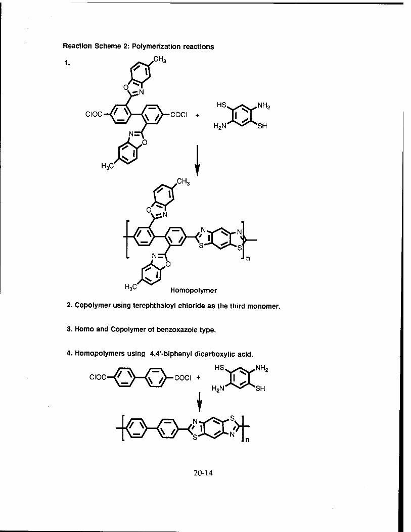
Reaction Scheme 2: Polymerization reactions

1. - 'CHa

HSÄ' HSW ^r^ ^NH2

OCX-

Homopolymer

2. Copolymer using terephthaloyl chloride as the third monomer.

3. Homo and Copolymer of benzoxazole type.

4. Homopolymers using 4,4'-biphenyl dicarboxylic acid.

20-14

c 3

">s C u CX

IS

c o c ao c

"5 o

x:

-a c o ex E o u

13 •o o

o

c o

3

U 3 ex

a Ui 3 SO

20-15

- 86'

»611

5SH

C u JS o. IS

o N

X o N C

I «3

> S9Ct I

O E 8

OZS! 3 fa O

0Ä

3

S"Z* (TO* 0"SC S'lJ (TOE S'iZ 0"or r:x

20-16

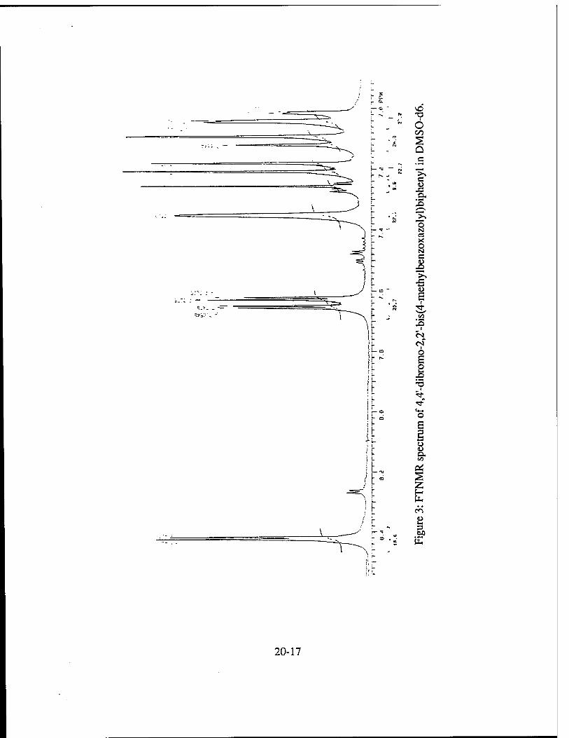
It

vO •o I

O e/5

Q

c u J3 OH

o SI es

o N C

!

•s

I o

X! -5

i

■<sf

It o u GO

Cd

Z

en s 3

20-17

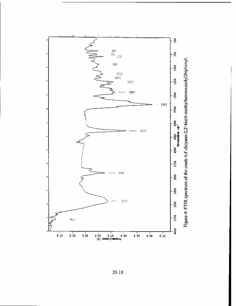
c

"E. J5

o N «J X o N c

■>»

6 I

•-■<

X) i

fM

I O § o

'"£

5 o u

o u OH

Cd

2

9'iS O'SS S-JS O'OS S-i* o*s» s-:» <rot S"i£

20-18

c

s* IS

s 03 X. o N C

£ ■

■

i

X o >1 c3

5 o

o u

Cd

e

0"0i S":9 C"S9 S"J9 0"09 S"iS 0"SS S"ZS CCS S"i* ITS* r;f 0'0» S'iE [*] soüwrmstrerj,

20-19

S'i» 0"s» s*z* c [H] 9SCK3THSII8;,

0'S£

20-20

A FRAMEWORK FOR MANUFACTURING-ORIENTED, DESIGN-DIRECTED COST ESTIMATION

Allen G. Greenwood Associate Professor

Department of Industrial Engineering

Mississippi State University P. O. Box 9542

125 McCain Engineering Building Mississippi State, MS 39762


Wright Laboratory / Manufacturing Technology Directorate Manufacturing and Engineering Systems Division



and

Wright Laboratory Wright-Patterson Air Force Base, OH

September 1996

21- 1


Allen G. Greenwood Associate Professor

Department of Industrial Engineering Mississippi State University

ABSTRACT

Defense system requirements have shifted from performance at all costs, to one of ensuring

superiority, yet being affordable. As a result, affordability has become the primary focus of weapon

system procurement. In order to develop affordable products, product design and manufacturing

process design must be considered concurrently and early in the design phase. One approach to

developing affordable systems is to combine the integrated product/process development (IPPD)

process and virtual manufacturing (VM), or "manufacture in the computer." However, if product and

process design issues are to be effectively considered, then cost, schedule, and risk assessment tools

must be sensitive to changes in the product's physical design as well as to changes in the manufacturing

system. Unfortunately, such tools are not available today. However, this deficiency provides an

opportunity to totally rethink or "re-engineer/re-design" manufacturing cost estimating methodologies.

But, before "designing" and developing cost estimating methodologies that adequately address

affordability issues, effectively support the IPPD process, relate product and process variables, operate

in a virtual design environment, and model manufacturing and non-manufacturing indirect activities,

the progression of modeling, analysis and costing — from the individual features of the product being

designed to its impact on the enterprise — needs to be understood. This research provides a framework

that defines the modeling and analysis progression from product features to an enterprise view of the

production of the product. The framework provides the foundation for manufacturing-oriented, design-

directed cost estimating (MODDCE).

21- 2


Allen G. Greenwood

INTRODUCTION

In the 21« Century, technologically superior Air Force weapons systems will be produced for half of the cost and fielded in half the time through a fully integrated commercial, military and organic industrial base. The existing fleet will be upgraded and/or modified to maintain its superiority with the same reductions in cost and time. ([1], p. i) The environment for today's cost estimator and analyst is certainly very challenging. Computerization, software, robots, composites, uncertainty, and integrated systems all challenge the applicability of our existing tools and techniques. (R. R. Crum, [2])

In most commercial and defense industries today, the focus is on affordability. Affordability is

defined as the balance among requirements, costs, and budgets and considers both product performance

and cost. A technology is considered affordable if it meets the customer's requirements, is within the

customer's budget, and has the best value among available alternatives ([3], p. 2). This paper provides a

framework for addressing both product and process cost issues, during the design phase. Before

defining the framework, this section briefly provides the background, context, and motivation for this

research, in terms of the current military design and manufacturing environment and state of the art in

manufacturing cost estimating.

The Military Design and Manufacturing (and re-manufacturing) Environment

Any management system is affected by both a general environment and an operating

environment. The general environment includes basic economic, social, political, and legal pressures

that are brought to bear upon the firm or industry. More specifically, companies and industries must

function in an operating environment that includes customers, suppliers, competition, government,

technology (both internal and external) and the organization or management system itself. One of the

primary characteristics of today's general business environment is change. The defense industry, like

many others, is experiencing a period of rapid change. The change in the DoD's missions and needs is

driven by a shifting and uncertain threat environment, e.g. collapse of the Soviet Union, strong

downward fiscal pressures. As a result, affordability has become the primary focus of weapon system

procurement. Defense system requirements have shifted from performance at all costs, to one of

ensuring superiority, yet being affordable. DoD is adopting "a more balanced cost of performance view

where weapon system life cycle cost is viewed as an independent variable, not simply fall-out as a

dependent variable." [4]

The focus on affordability has led to widespread acquisition reform, utilization of integrated

product teams (IFTs), application of an integrated product/process development (IPPD) process or

21- 3

concurrent engineering, adoption of commercial practices in military production, military production on

commercial lines, emphasis on sustainment (stretching the life cycle of weapon systems through

modification and re-manufacture), etc. Few new major weapon system programs are expected in the

foreseeable future and those programs that are developed will mostly be procured in low production

volume and at a low production rate; in some cases, e.g. missiles, there will be low volume and a high

product mix. Many weapon system components have no commercial counterpart and, due to the highly

complex nature of the components and their low production volumes, many of the military's needs can

not "compete" in the broader global market. Obviously, these current and future trends all present

major challenges to the design and manufacture of superior yet affordable defense systems.

Affordability, a key metric in defense system acquisition and operation, considers both cost and

performance and is obtained and maintained by (1) identifying and assessing cost drivers early in the

life cycle, (2) considering process design and manufacturing operations early in the product life cycle,

(3) effectively linking product and process design, especially in terms of cost, schedule, and risk, and

(4) managing cost and risk over the system's entire life cycle. While affordability assessments need to

address all phases of the product's life cycle, and the costs that will be incurred in those phases, i.e. life

cycle cost, this project focuses only on the costs incurred in the production phase and the design and

operation of manufacturing systems.

One vehicle for addressing affordability, and other issues, is through IPTs and the IPPD process.

The IPTs must concurrently consider, either in person or over computer networks, product design and

manufacturing process design in terms of product performance and cost tradeoffs. The largest payoffs

result from effectively utilizing IPTs as early as possible in the design phase. The importance of early

design decisions is widely recognized. It is often stated that roughly 70 percent of the total life cycle cost

of the system is determined during conceptual design [5].

The relationships between the business and operating environment, the IPPD process, the

concurrent consideration of product and process design, and the tradeoffs between cost and

performance is represented graphically in Figure 1.

The cost/performance tradeoff graphic at the bottom of Figure 1, a variation on a concept put

forth by Yoshimura [6], depicts the goal of design as seeking higher product performance and lower

process cost; i.e., driving the design toward the "efficient frontier." The efficient frontier, the edge of the

feasible region in Figure 1, contains the Pareto optimum design solutions — those solutions where there

exists no other feasible design solution that will yield an improvement in one objective without causing

degradation in the other objective. Cost estimating methodologies are generally grouped into four

categories [7]: (1) judgment - use of expert opinion of one or more qualified experts in the area to be

estimated, (2) parametric — mathematical expressions, often referred to as cost estimating relationships

or CERs, that relate cost to independent cost driving variables, (3) analogy - use of actual costs from a

similar existing or past programs with adjustments for complexity, technical or physical differences, to

21- 4

derive a new system estimate, and (4) grass roots, also referred to as "engineering build up" or "detailed

estimate" are performed at the functional level of the Work Breakdown Structure.

-gs^4s^f«;SSSg«^^

Social Political Legal

Technology Olganization

Si?

8

O— *W- frJESXn-) OfcSw G°™tt COmpeÜti0n

.-;■■■ ' Opg*nt '^^^^"^^^^-^^■^v^^^^ ^"^TS^"^ i.v^^'l?^^^^^^^

Integrated Product/Process

Development

o U '^L- -—-*~ •gfcyff

rtrforrnvKc

Figure 1: Affordability is the driving force in today's defense manufacturing environment.

One way to develop affordable products is through virtual manufacturing (VM), or

"manufacture in the computer." VM is one of the key technologies which allows defense manufacturers

to go beyond the assumptions driving the historic acquisition process because it provides four

fundamental changes for defense manufacturing [8]: (1) VM can be used to prove the production

scenarios, resulting in "pre-production hardened systems"; (2) VM can support the generation of more

reliable estimates of production costs and schedule because the models are based on actual processes,

not just parametrics; (3) modeling and simulation can significantly improve production flexibility, hence,

reducing the fixed costs; and, (4) reliable predictions of costs, risk, and schedule can substantially

improve the decision making process of acquisition managers.

In this new and evolving technology, fabrication and assembly of any product, including the

associated manufacturing processes and all variables in the production environment from shop floor

processes to enterprise transactions, are modeled and simulated in an integrated computer environment.

VM accommodates the visualization of interacting production processes, process planning, scheduling,

assembly planning, logistics from the line to the enterprise, and related impacting processes such as

21- 5

accounting, purchasing, and management [9]. The move from solid models to virtual environment

enables manufacturing and industrial engineers to design, test, and modify manufacturing processes

without physical prototypes or production interruptions. It allows integrated product and process

development (IPPD) in a virtual, 3-D world that is understood by all participants in the product and

process design. ([10], pp. 35-36)

In order for IPTs to effectively consider product and process design issues, they need cost,

schedule, and risk assessment tools that are sensitive to changes in the product's design, as well as to

changes in the design of the manufacturing system. Unfortunately, such tools are not available today. A

review by Thomas [11] of papers published in major journals in the past five years, resulted in the

following conclusions: (1) research in manufacturing cost estimation has involved rather few people and

as a result there are no broadly applicable mathematical models, (2) there is widespread dissatisfaction

with the way overhead or indirect costs are handled, and (3) the lack of broadly applicable cost models

leads to few efforts directed towards their integration into the CAD/IPPD systems.

Many cost models do not provide the capability to perform meaningful product/process trades

and, in fact, may lead to an inefficient improvement focus. For example, many existing cost models are

driven by parameters such as weight. As Dean [12] points out, "there are many perceptions of cost

which people believe to be true and act upon, but which leads us in the wrong direction. ... The weight-

based cost estimating relationship, as are many other common perceptions of cost, is quite misleading

unless fully understood from a cost perspective and an engineering perspective." This is illustrated in

Figure 2, using data from the Manufacturing 2005 Program ([13], [14]). In this case, if a design goal is to

reduce manufacturing cost of the horizontal stabilizer and if CERs that are based on weight are used in

the analysis, then the design focus would be on the stabilizer's skins. As seen in the table below, each

skin comprises approximately one third of the weight of the structure and accounts for about one fifth of

the cost. However, the ribs account for more than one third of the manufacturing cost but comprise less

than ten percent of the weight.

Based on the research conducted during this project, the author adds the following issues to the

list of concerns with the current state of manufacturing cost estimating in the IPPD process: (1) Cost

model drivers need to be more closely related to the characteristics of manufacturing processes and

operations. The process needs to be designed as much as the product; all too often the product is

designed and then the process (manufacturing) must be designed to accommodate it or the product

must be redesigned to accommodate the process. (2) Cost model drivers need to be more closely related

to product features. (3) Manufacturing process design and resulting costs need to be considered earlier

in the design of the product. (4) Product and process design must be sensitive to the existing or planned

manufacturing state, especially in an agile environment; i.e. a design may change based on current

factory utilization. Cost models need to capture the dynamics and stochastic nature of manufacturing.

(5) The relationship between product/process costs and indirect costs need to be better defined and

21- 6

understood. Indirect costs, both manufacturing and non-manufacturing, need to be "modeled" so that

they can be addressed during design. (6) Legacy cost system data are often not tracked at the level of

detail needed in design. (7) Legacy cost system data are often based on processes and methods that are

no longer used.

Weight Putt Bastenen Tool» Labor Material $ S

Upper akin

Lower skin

Bronx tpai

Read spar

Rika Box Assembly

Other

llllpgASs 12.« 11; !::;';S;33.'" IM II'

».» 10.»

».7 4»

».» pSS»:' 11 5.1

L» 0.0

Süll 235

lt.*

I.(

M.1 |

7.6

0.0

1X0

».» «.( 7.0

■;WJ • 5.7"

ai

Mann£ Coat

15.7 ;i;;i:SäÖSSs!!tÜ|

.„.„... ^

«.• 7.7

U.0 >_:■»«»«*;

0.0 fci

131 ■■■

7J

»X 1.0

Source: Fordon. I. W. Jr. D. Rasjnussen. et aL (1S%> larg* Compos* Slmrttf« - Cwmwrc«: Miitoy Inky/atam (M«wy Pro*«* Uatie fcW C«mBfrt»I Prart«) Plate I -Aton^eaiTwr 2005 Bvimm Prarit» ifcm^öwwr WJMhweau^ Prooe» T«*»otojyDmqn« Vota«U-MnvM™S »OSitontoo». Whf^t Jattmon Air Fon* Bast, OK Marnifaet-mng Technology Directorate Wnght laboratory. AirForceMatene! Cflnwatl p. EW. 3&

Figure 2: Many weight -driven cost models do not permit meaningful product/process trades.

Despite the shortcomings of past and current cost estimating methodologies and the lack of

perceived value that they provide to the IPPD process, there are research efforts underway that are

attempting to mitigate these problem; some of those efforts will be identified later in this report. It seems

that if we can model and simulate the operation and behavior of a product and process, we certainly

should be able to model and simulate a product/process's cost behavior. In fact, VM provides an

opportunity to "re-engineer" costing methodologies. We need to freshly examine how costing should be

done in a virtual environment, unencumbered by traditional accounting practices. New costing

methodologies need to be designed to fit into tomorrow's environment.

But, before "designing" and developing cost estimating methodologies that adequately address

affordability issues, effectively support the IPPD process and relate product and process variables,

operate in a virtual design environment, and model manufacturing and non-manufacturing indirect

activities, we need to understand the progression of modeling, analysis and costing from the individual

features of the product being designed to its impact on the enterprise. The result of this research study is

a framework that defines the modeling and analysis progression from product features to an enterprise

view of the production of the product. The framework provides the foundation for manufacturing-

oriented, design-directed cost estimation (MODDCE).

THE MODDCE FRAMEWORK

An overview of the manufacturing-oriented, design directed cost estimating (MODDCE)

framework that was developed as part of this research study is provided in Figure 3. The framework is

21- 7

composed of five levels that progress from a hierarchical decomposition of a product's features through

three intermediate steps to an enterprise-level model that links product features with manufacturing

and non-manufacturing entities throughout the enterprise. The highest or enterprise level provides the

most comprehensive analysis capabilities for assessing the effect of changes in product and process

design on the enterprise and the resulting effect of those changes on "total" cost. The progression to

each level requires the completion of an activity. For example, in order to move from the hierarchical

decomposition of a product's features to the corresponding manufacturing elements that create those

features, requires an activity that maps or associates features with transformation elements. Each of the

activities that link the five levels are described in the following sub-sections.

Decomposition of kerns/Features

Entwprts« Modal

Enterprise Cost

Manufacturing Elements

Transformations of snap« and properties

Manufacturing Operations

Manufacturing Process Objects

Mfg. System

Elemental Cost

\^E" Operations Cost *»

sZ— rrr—sj

SystwnCost

g*^

Figure 3: MODDCE framework provides the basis for "designing" and integrating costing methodologies that link product features to an enterprise view of the production of the product.

A preliminary and partial data model for implementing the MODDCE framework is provided

in Figure 4. The data model is described in the framework subsections that are most closely related to

each data model entity. As a matter of notation, lines with no double-headed arrows indicate a one-to-

one relationships between entities, a double-headed arrow on one end represents a one-to-many

relationship, and arrows on both ends represents a many-to-many relationship. For example, there is a

many-to-many relationship between suppliers and items - an item may be obtained from multiple

suppliers and a supplier may provide many items to the company. Also, there is an implied inheritance

of information from entity to entity, as one moves from left to right in Figure 4; i.e., a manufacturing

process object inherits all of the information about manufacturing operations, manufacturing elements,

and product feature characteristics.

21- 8

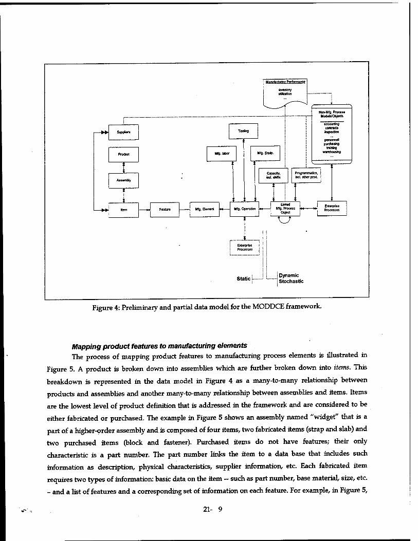
Manufacturing Performance

inventory utKzation

Suppfere Toofing

Mfg. labor

Assembly

->► H Mfg. Element «+■

Mfg. Equip-

Non-Mfg. Process Models/Objects

accounting

contracts

personnefl

purchasing training

warehousing

Capaefty,

incL shifts

Programmaties,

incl. other prod.

Mfg. Operation

Linked Mfg. Process (M **

Object

XT Enterprise Processes

Enterprise

Processes

Static ?• Dynamic Stochastic

Figure 4: Preliminary and partial data model for the MODDCE framework.

Mapping product features to manufacturing elements The process of mapping product features to manufacturing process elements is illustrated in

Figure 5. A product is broken down into assemblies which are further broken down into items. This

breakdown is represented in the data model in Figure 4 as a many-to-many relationship between

products and assemblies and another many-to-many relationship between assemblies and items. Items

are the lowest level of product definition that is addressed in the framework and are considered to be

either fabricated or purchased. The example in Figure 5 shows an assembly named "widget" that is a

part of a higher-order assembly and is composed of four items, two fabricated items (strap and slab) and

two purchased items (block and fastener). Purchased items do not have features; their only

characteristic is a part number. The part number links the item to a data base that includes such

information as description, physical characteristics, supplier information, etc. Each fabricated item

requires two types of information: basic data on the item — such as part number, base material, size, etc.

- and a list of features and a corresponding set of information on each feature. For example, in Figure 5,

21- 9

the fabricated item "slab" has three features, two holes and one surface characteristic. Hole features

would contain such information as diameter, depth, tolerance, location, etc. and surface features would

contain such information as the face that is treated, purpose of treatment, material, etc.

Once all of the items have been defined and their features specified, a manufacturing element

that creates the feature, either by transforming the shape of the item or altering its properties (non-

shaping), is specified. There is a one-to-one relationship between a feature and an element. Elements are

specified from a taxonomy of manufacturing processes, e.g. [15]. The element specification may be for a

specific manufacturing process or for a more general process family. The choice of a manufacturing

process is dictated by various considerations ([16], p. 1232): characteristics and properties of the

workpiece material, shape, size, and thickness of the part, tolerances and surface finish requirements,

functional requirements for the expected service life of the item, production volume and schedule, level

of automation required to meet production volume and rate, costs involved in individual and combined

aspects of the manufacturing operation. Numerous guidelines are available on the capabilities of various

manufacturing processes for producing items from different materials, shape characteristics, tolerance

and shape characteristics, etc. Some guidelines are incorporated into CAD software to provide real-time

feedback to the designer. Cost guidelines are also available, usually on a relative basis. All too often

these guidelines represent general trends and are not related to specific processes and product features.

Few guidelines are available on the cost impact of production volume, rate, lead time, etc. These are

factors that are becoming increasingly important to address during design especially when fewer new

defense systems are being procured and there is a growing need to sustain and re-manufacture systems

that are no longer being procured.

Using the Todd et al. taxonomy [15], a hole requires a shaping manufacturing process that could

be either mass reducing or mass conserving. If a hole is created by mechanical mass reduction, further

specification would require consideration of manufacturing processes that are chip-oriented (e.g.

drilling) or shear-oriented (e.g. blanking). Alternatively, a hole could be created through a mass

conservation process which may involve a consolidation process, such as casting, or a deformation

process, such as forging. As shown in Figure 5, for the widget example, the hole features in the slab and

straps are specified very generally; they are only identified as being mass reduction elements. On the

other hand, the surface property of the slab in Figure 5 is specified more precisely as being a charge-

transferred spray coating. Note that at this level of analysis, even if the methodology used to create the

feature is precisely specified, such considerations as setup, simultaneous operations, resource

availability, etc. are not considered.

Specification of manufacturing elements provide the first opportunity for cost assessment.

However, in order to provide a cursory assessment of cost, a default manufacturing process would have

to be associated with each element, e.g. the manufacturing process drilling could be Hie assumed

process used to create a hole. Since each element is discrete and disjoint, it is more appropriate to begin

21- 10

costing at the next level, the operations level. The transition to the operations level requires combining

elements related to each feature into manufacturing operations; this activity is described in the following

section.

ckufl] - F*i_»a, Material, height, vridli, thicltae», weight,. cbafft] ■ diameter, depth, tolerance, locatioa, ... duiJ3] ■ face, nuten*!, — cha*(4] - p*rt_*o., ...

»-fabricated item H* » pwrchascd Hen

Figure 5: Mapping product features to manufacturing elements.

Combining manufacturing elements into operations The second activity combines manufacturing elements for each feature, as described above, into

manufacturing process operations. An illustration of this activity using the widget example is provided in

Figure 6. The oval-shaped symbols in the figure represent manufacturing operations. As can be seen in

Figure 6, the strap item is produced by stamping - the base material is cut to size and the two holes are

formed in one step using the stamping process. Note that the creation of several feature elements have

been combined in order to form the stamping operation and that the manufacturing process for creating

the features has become more specifically defined, from the general mass reduction process family

specified for the manufacturing elements to the particular process, stamping, specified as a process

operation. It is at this level that specific equipment, labor skill requirements, and tooling are designated,

as illustrated in the data model in Figure 4, where the manufacturing operations are linked to

equipment, labor, and tooling data files. It is also at this level where precedence among elements and

operations is defined. The dashed lines in Figure 6 indicate precedence; for example, for the slab item,

the base material is cut first, then painted, and finally the holes are created through drilling.

21- 11

Based on the research conducted during this study, this level of analysis is the current state of

the art in cost estimating methodologies that directly link product features to process characteristics.

Development of this capability is a part of two JSF/J AST projects. The Joint Strike Fighter (JSF) program,

formerly the Joint Advanced Strike Fighter OAST) program, is chartered to develop an affordable next-

generation strike weapon system for the Navy, Marine Corps, Air Force, and our allies. Both projects -

JMD, JAST Manufacturing Demonstration (prime contractor: Hughes Aircraft Company) and SAVE,

Simulation Analysis Validation Environment (prime contractor: Lockheed Martin Tactical Aircraft

Systems, LMTAS) - link feature-based CAD software (Pro/E and CATIA, respectively) to Cognition

Corporation's Cost Advantage (CA) software system. CA is a design for manufacturing expert system

that provides design guidance, manufacturing alternative analysis, producibility analysis, and predictive

cost analysis. CA uses process models that are comprised of information and rules to estimate costs and

advise engineers on the manufacturability of product designs. As part of this research program, the

author met with engineers from Cognition Corporation and LMTAS [17] in order to better understand

their development efforts.

However, in order to have a complete virtual manufacturing environment, the cost estimating

capability must be extended beyond this process-level analysis to the system level and ultimately to the

enterprise level. The following two sections describe these levels.

Manufacturing Elements

Transformations of shape and propertiaa

■^^

combine elements into process operations

Manufacturing Process

Operations

Elemental Cost Operations Cost

A . widget | assembly join

5-SKK I-F

■IBS I-F

strap hotel hold

slab hotel holeZ sutf_char

—> base material _> drill _> drill

base material drill drill paint

§|1| I-F | block

11111 I-F I fastener

material

— -/faltai J

Figure 6: Combining elements into process operations.

21- 12

Transforming process operations into manufacturing process objects The third activity moves the modeling and analysis capability from the process level to the

system level by transforming discrete process operations into system-level manufacturing process

objects. It is at this level, and through the use of the objects, that manufacturing process operations are

placed in the context of an actual production environment and the product is integrated into the fabric

of a manufacturing environment. As a result, the objects become the basis for the design of production

operations and facilities by considering such things as product movement, storage and handling issues,

resource availability, interference with other products, grouping of elements into cells, etc. The

combining of process operations into objects is analogous to implementing process plans into the

production environment. The application of process objects is illustrated by the facility layout in the

middle of Figure 7. In this case, continuing with the widget example, the strap item is created in the

press area; the slab is created by slitting, is then painted, and fabrication is completed in the cell prior to

assembly with the other items.

The symbols at the bottom of Figure 7 illustrate the differences between process operations and

process objects. Process operations consider both the procedures (manufacturing steps) and the human

and equipment resources that are required to perform the specific manufacturing activities. For

example, the stamping process operation identifies the type of machine and operator that are needed to

do the stamping, as well as the time required per item. As shown in the process object symbol in

Figure 7, objects also consider procedures and resources but in addition they consider movement and

storage of the product between and within objects, machine and operator capacities, programmatics,

interaction with other products, and interaction among resources. Also, process operations are static;

whereas, process objects are dynamic and stochastic - both of which are characteristics of most

manufacturing systems. That is, process objects are time sensitive and have the ability to incorporate

random events. Process objects obtain most of their power from imbedded methods, such as scheduling

algorithms, simulation, etc.

It is only through manufacturing process objects and the interaction among objects that

manufacturing performance, including costs, can be evaluated. The object provides output regarding

both the expected value and distribution of such measures as completion times, throughput, operator

and machine utilization, work-in-process inventory, space requirements, etc. System-level analysis

provides a means to identify bottlenecks and other potential problems before the product is committed

to production. It is only at this level that the impact of a product's characteristics on production process

can be assessed and evaluated. This is especially important in an agile environment or for

accommodating small batches of dissimilar products (e.g. items for the defense industry be produced on

commercial lines). In fact, the design of the product may change based on the current state of the

manufacturing facility, e.g. available resources, supplier constraints, etc.

21- 13

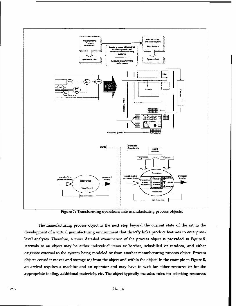
Manufacturing

Operations

Operations Cost

Create process objects that simulate dynamic and

stochastic manufacturing systems

> Manufacturing

Process Objects

Mfg. System

measure manufacturing performance

System Cost

3=£ ]S>--<£>-

Finished goods ♦

Static

operations) or processed ftem(6)

I Dynamic 1 Stochastic invwietv

tfjkza&oti boeMrwcks

operation^) Of processed item<s) j

Figure 7: Transforming operations into manufacturing process objects.

The manufacturing process object is the next step beyond the current state of the art in the

development of a virtual manufacturing environment that directly links product features to enterprise-

level analyses. Therefore, a more detailed examination of the process object is provided in Figure 8.

Arrivals to an object may be either individual items or batches, scheduled or random, and either

originate external to the system being modeled or from another manufacturing process object. Process

objects consider moves and storage to/from the object and within the object. In the example in Figure 8,

an arrival requires a machine and an operator and may have to wait for either resource or for the

appropriate tooling, additional materials, etc. The object typically includes rules for selecting resources

21- 14

or for the resources to select products. Activity times, both machine and operator, are stochastic and

sampled from probability distributions. Also, resources used by objects are not always available, due to

scheduled or unscheduled maintenance, shift schedules, etc. Objects also include the modeling of the

disposition of scrap and re-work. It is only through the dynamic and stochastic capabilities of the

manufacturing process object that a system's performance can realistically be evaluated and virtual

manufacturing can truly be achieved.

-Afrtvite:^

;,:j)rooB6* object m:,t

Figure 8: Example of a manufacturing process object.

Linking manufacturing process objects to enterprise processes The highest level of cost analysis is at the enterprise level. Enterprise-level costing extends

design sensitivity beyond direct manufacturing costs to include manufacturing and non-manufacturing

indirect costs. The impact of changes in product/process design on indirect entities in the enterprise is

assessed, and conversely, the impact of changes in indirect entities on manufacturing processes, and

hence on the product, is also assessed. For example, specification of a new material during product

design will not only affect operations in terms of the type of equipment used, labor skills, tooling, scrap

rate, etc. but will also affect numerous indirect entities in the organization, including training,

purchasing, warehousing, etc. Normally these effects are assumed to be captured in the application of

very general overhead rates. However, enterprise-level costing permits a more realistic assessment of

the impacts of product and process alternatives. In order to realize enterprise-level cost estimation, the

firm's business processes must be identified, modeled, and linked to the appropriate manufacturing

process object(s). This is illustrated in Figure 9 with the links between various functional entities in the

organization. Also, as illustrated in Figure 9, enterprise is defined in its broadest context and includes all

non-manufacturing entities in the company (administration, purchasing, etc.), as well as external entities

such as customers and suppliers.

21- 15

CUSTOMERS

Figure 9: Enterprise-level analysis links indirect entities with direct manufacturing objects.

An example of a model of a business process is provided in Figure 10; the supplier management

and procurement process was developed as part of the Manufacturing 2005 Program [13]. The process

model illustrates the linkages between manufacturing and such entities as program management,

engineering, quality assurance, the supplier, etc.

Source: Fondon, J. Wv Jrv D. Rmnwn, «t «1. (1996J. large Cmtpotik Strucbae - Cmmcrcml MäUgry Intqnwtkm (MUthay JYozarfe Uro; Bar C»mr<mirffrarfi«s; Phase 7 ~Mirm^ Pmcat Ttdmrtogtf Oepdopmtnt, Vahpnc Ü - Manufacturing 2005 Hanähcck. Wright-Pattmon Air Force Base, OH, Manufacturing TVthnotoRy Directorate, Wright I aboratory. Air Force Materiel Command, p. B-16.

Figure 10: Example linkage between business and manufacturing processes.

21- 16

As mentioned above, enterprise-level modeling and analysis results in a better understanding

and a better definition of the behavior of overhead costs. Overhead costs are a significant component of

total product cost. Raffi and Swamidass [18] report that in an average U.S. manufacturing firm,

manufacturing overhead cost is about two and one half times the direct labor cost. Thomas [11] reports

indirect costs to be 400 to 600 percent of direct costs in aerospace defense production. Despite the

significance of overhead costs, little published research exists in this area. The MODDCE framework

provides a foundation for modeling non-manufacturing processes and quantifying the effect of a

process's behavior on overhead cost. New accounting methodologies, such as activity-based costing

(ABC), will be required in order to model and link direct and indirect processes.

As part of this research project, the author visited the Northrop Grumman Commercial Aircraft

Division (NG-CAD) in Dallas, TX in order to gain a better understanding of the costing and risk

assessment methodologies used in the Manufacturing 20005 Program, Military Products using best

Commercial/Military Practices (MP-C/MP) [19].

Development of an Application of the MODDCE Framework This research project provides a framework for manufacturing-oriented, design-driven cost

estimating. Subsequent research will develop an application to implement the framework. This section

provides a brief and preliminary definition of the application.

As shown in Figure 11, a decision-support application that implements the MODDCE

framework would include, at a minimum, the seamless integration of: relational and/or object-oriented

database(s), a mechanical CAD package for product design (e.g. Cognition Corporation's Mechanical

Advantage, Parametric Technology Corporation's Pro/E), process and cost modeling system(s) (e.g.

Cognition Corporation's Cost Advantage), manufacturing process objects that would most likely be

developed from manufacturing and/or object-oriented simulators (e.g. AESOP's SIMPLE++, ProModel

Corporation's ProModel), and business modeling and simulation software (e.g. CACI's SimProcess,

ProModel Corporation's ProcessModel, AdvanEdge Technologies Corporation's OPTIMA!). These

components would be integrated using software such as Microsoft Visual Basic and/or Knowledge Base

Engineering's IKE (Integrated Knowledge Environment). The application would be developed in a

Microsoft Windows environment, most likely Windows NT.

Development of manufacturing process objects, development of the underlying database

structure, modeling of business processes, integration of the technologies outlined above, and design of

the user interface and decision-support environment would be required to effectively link product

features and characteristics to manufacturing and enterprise-wide processes. The application would

support the modeling of information flow as well as product and material flow. Costing methodologies,

e.g. activity-based costing, need to be investigated in order to determine their applicability to this

21- 17

environment and identify the best way to integrate the costing methodologies into the

framework/application.

Figure 11: Application software for implementing the framework.

FUTURE RESEARCH ISSUES

As defined in the previous section, the next research activity is to begin the development of a

prototypical application that demonstrates the proposed framework. This completed prototype will

provide a laboratory for exploring a variety of issues related to cost estimating in an integrated

product/process development environment and virtual design and manufacturing environments. Some

of those issues include specification of the most appropriate costing methodologies for assessing both

direct and indirect costs, the application of activity-based costing, application of machine learning,

development of approaches for optimization of product/process design via simulation, etc.

Another area for further research, which would directly support the application development

defined above, is the generalization and extension of the "innovative" costing work performed in

support of the Manufacturing 2005, MP-C/MP (Military Products Using Best Commercial/Military

Practices), Program ([13], [14]). One of the outcomes of the MP-C/MP Program is a detailed assessment

21- 18

of the impact of numerous business practice, manufacturing infrastructure, and process technology

improvement initiatives on product and process costs. The program clearly demonstrates that indirect

cost categories can be linked to product and process characteristics. The MP-C/MP Program cost

methodologies provide a basis for process modeling and linking manufacturing and non-manufacturing

activities.

A third research project would involve the development of an industry "survey" or workshop

that would determine and define the cost estimating needs for a virtual design environment. The project

would solicit ideas on how cost estimating should be performed in such an environment.

CONCLUSIONS

Realization of the proposed framework would advance the state of the art of manufacturing cost

estimating methodologies in the following ways: (1) Product design is directly linked to process design

and manufacturing operations, thereby achieving "true" virtual manufacturing. Shop-floor and above-

the-shop-floor assessments are performed in the computer before commitments are made to produce a

product; e.g. potential bottlenecks can be identified and resolved before they occur. (2) Product and

process design are directly linked to non-manufacturing activities in the enterprise, resulting in a more

accurate and more meaningful assessment of indirect costs. (3) Product/process designs are assessed

and "optimized" at the system level, rather than sub-optimized by functional area. (4) The framework is

applicable throughout the product and process life cycles, thereby providing traceability of product

design, manufacturing design, and cost. It also provides a growing knowledge base of past practices and

lessons learned to be used in future designs. (5) The aforementioned knowledge base can be used not

only for human learning, but as a basis for machine learning - a means to analyze and "optimize" the

relationships between product features and the processes required to produce those features.

(6) Product/process trades are made on "current" planned activities. This is especially important as the

design cycle time shrinks - current activities and plans for the facility may impact the selection of

product/process design alternatives.

BIBLIOGRAPHY

1. Air Force Manufacturing Science & Technology Program. FY96 Manufacturing Science and Technology Area Plan. Wright-Patterson Air Force Base, OH: Headquarters, Air Force Material Command, Directorate of Science and Technology, August 1,1995:

2. Kankey, R. and J. Robbins, eds. Cost Analysis and Estimating: Shifting U.S. Priorities. New York: Springer-Verlag, 1991.

3. Wright Laboratory Affordability Strategy Team. AffbrdaUlity in Science and Technology Development. Wright-Patterson Air Force Base, OH: Wright Laboratory, June 9,1993.

21- 19

4. Kaminski, P.G. The Defense Acquisition Challege: Technological Supremacy at an Affordable Cost. JAST Industry Conference, 1995.

5. Dierolf, D.A. and K.J. Richter. Computer-Aided Group Problem Solving for Unified Life Cycle Engineering (ULCE) Environment. IDA Paper P-2149, Alexandria, VA: Institute for Defense Analyses, 1989.

6. Yoshimura, M. Concurrent optimization of product design and manufacture, in Concurrent Engineering: Contemporary issues and modern design tools, H.R. Parsaei, Editor. London: Chapman & Hall. 1993, pp. 159-183.

7. Modern Technologies Corporation. Integrated Weapon Systems Management (IWSM) "How to" Manual for Manufacturing Cost Assessment (MCA). Dayton, OH: Modern Technologies Corporation, 1995.

8. Lawrence Associates, Inc. Virtual Manufacturing Use? Workshop. Dayton, OH, 1994.

9. Lawrence Associates, Inc. Virtual Manufacturing Technical Workshop. Dayton, OH, 1994.

10. Noor, A.K. and S.R. Ellis. Engineering in a Virtual Environment. Aerospace America, July 1996, pp. 32-37.

11. Thomas, R. Manufacturing Cost Estimation, Modeling and Control: A Review of the Literature. Beavercreek, OH: Stratech, Inc., August 1994.

12. Dean, E. Design for Competitive Advantage, Internet, Hampton, VA: NASA Langley Research Center, 1996.

13. Fondon, J.W., Jr., Rasmussen, Dane et al., Large Composite Structure — Commercial Military Integration (Military Products Using Best Commercial Practices) Phase I — Manufacturing 2005 Business Practices, Manufacturing Infrastructure, Process Technology Development, Volume II — Manufacturing 2005 Handbook Wright-Patterson Air Force Base, OH: Manufacturing Technology Directorate, Wright Laboratory, Air Force Materiel Command, 19%.

14. Riseley, M.K., T. Houpt, and S. Wheeler, Large Composite Structure — Commercial Military Integration (Military Products Using Best Commercial Practices) Phase I — Manufacturing 2005 Business Practices, Manufacturing Infrastructure, Process Technology Development, Volume I — Program Review. Wright-Patterson Air Force Base, OH: Manufacturing Technology Directorate, Wright Laboratory, Air Force Materiel Command, 1996.

15. Todd, R.H. et al, Manufacturing Process Reference Guide. New York: Industrial Press Inc., 1994.

16. Kalpakjian, S. Manufacturing Engineering and Technology. Reading, MA: Addison-Wesley Publishing Company, 1992.

17. Greenwood, A.G., Meeting on SAVE Program at LMTAS, 7/1/96. Wright-Patterson Air Force Base, OH: Manufacturing Technology Directorate, Wright Laboratory.

18. Raffi, F. and P.M. Swamidass. Towards a Theory of Manufacturing Overhead Cost Behavior: A Conceptual and Empirical Analysis. Journal of Operations Management, October 1987 pp. 121-137.

19. Greenwood, A.G., Meeting on Manufacturing 2005 Program at NG-CAD, 7/2/96. Wright-Patterson Air Force Base, OH: Manufacturing Technology Directorate, Wright Laboratory.

21- 20

AFFECTS OF INTERNATIONAL QUALITY STANDARDS ON BARE BASE WASTE DISPOSAL ALTERNATIVES

Rita A. Gregory Assistant Professor

School of Civil and Environmental Engineering Construction Engineering and Management

Georgia Institute of Technology Atlanta, GA 30332-0355


Wright Laboratory Air Base Technology Branch

WL/ FIVC-OL



and

Wright Laboratory Air Base Technology Branch

WL/FIVC-OL

September 1996

22-1


Rita A. Gregory Assistant Professor

School of Civil and Environmental Engineering Construction Engineering and Management

Georgia Institute of Technology

Abstract

This research was sponsored by the Air Force Office of Scientific Research,

Boiling AFB, DC and the Air Force Wright Laboratory Air Base Technology Branch

(WL/FIVC-OL Tyndall AFB, FL) as part of the Summer Faculty Research Program.

This research was designed to assist Wright Laboratory Air Base Technology Branch in

identifying emerging technologies for the development of a versatile, air mobile, and

environmentally safe waste processing system to support force deployment operations. In

addition, a specific thrust of this researcher is to develop cost/benefit methodologies and

to incorporate in the alternative development processes those aspects of engineering,

socio-economic, and policy issues that could impact the cost effectiveness of alternative

solutions. This final report discusses some of the issues that International Quality

Standards could have on the design and cost effectiveness of Bare Base Waste Disposal

Alternatives. Although these standards are still under development and there are not yet

definitive policies (14, 15) on how the DoD will integrate these standards into their bare

base deployments, a DoD wide Environmental Management Systems Committee has been

formed. (14, 15) They will continue to evaluate the development of international

standards to determine if they present an "opportunity for DoD to improve its

environmental management," with a "primary motivation for (sic) regulatory relief and

reduced costs." (14) This researcher believes these standards will require us to process

waste more efficiently and environmentally sound, thereby provide solid ground to support

technology innovation under development and proposed by Wright Laboratories.

22-2


Rita A. Gregory

Introduction

This research was sponsored by the Air Force Office of Scientific Research,

Boiling AFB, DC and the Air Force Wright Laboratory Air Base Technology Branch

(WL/FIVC-OL Tyndall AFB, FL) as part of the Summer Faculty Research Program.

This research was designed to assist Wright Laboratory Air Base Technology Branch in

identifying emerging technologies for the development of a versatile, air mobile, and

environmentally safe waste processing system to support force deployment operation. In

addition, a specific thrust of this researcher is to develop cost/benefit methodologies and

to incorporate in the alternative development processes those aspects of engineering,

socio-economic, and policy issues that could impact the cost effectiveness of alternative

solutions. This final report for the Summer Faculty Research Program discusses some of

the issues that International Quality Standards-specifically ISO 9000, international

standards for manufacturing and construction and ISO 14000, international standards for

environmental management systems (l)--could have on the design and cost effectiveness

of Bare Base Waste Disposal Alternatives. Although these standards are still under

development and there are not yet definitive policies (14, 15) on how the DoD will

integrate these standards into their bare base deployments, a DoD wide Environmental

Management Systems Committee has been formed. (14, 15) Members of this committee

believe "ISO 14000 will have greater impact on international trade than the ISO 9000"

and "ISO 14000 will grow in importance over time." (14) They will continue to evaluate

the development of international standards to determine if they present an "opportunity for

DoD to improve its environmental management," with a "primary motivation for (sic)

regulatory relief and reduced costs." (14)

The U.S. Army Corps of Engineers (COE) say the quality (management) system

outlined under ISO 9002 is the standard most applicable to construction firms in the

22-3

private sector that support military construction. (16) The Louisville (KY) District is

attempting registration under ISO 9000 and is tracking the development of ISO 14000.

They say "Registration to the ISO 9000 standard demonstrates to our customers our

commitment to quality and our ability to meet their specified requirements and to possibly

exceed their service expectations. . . . ISO 9001 registration is a practical, commercial

requirement for world-wide business organizations." (17) The ISO standards in the

United States are known as ANSI/ASQC Q9000 series. (17)

International Standards are the way of the future for home bases and contingency

deployments. This researcher believes these standards will require Air Force Bare Bases

to process waste more efficiently and environmentally sound, thereby provide solid ground

to support technology innovation under development and proposed by Wright

Laboratories.

Background/Discussion of Problem

In the future, under the doctrine of "Global Reach... Global Power," the USAF is

preparing to fight world wide from 1100-person Bare Bases consisting of only operating

surfaces and a source of water. All other base infrastructure components must be rapidly

brought via airlift. The USAF tasked Sverdrup Technology, Inc., TEAS Group with

developing the "Bare Base Infrastructure Road Map," identifying deficiencies and defining

promising technologies available in 1996 to 2015 for improving current austere base utility

and facility equipment. Inadequate Waste Management Systems was one of the top ten

deficiencies identified in this study. Several of the top priorities for immediate action

recommended by the study were to quantify and characterize waste streams and

investigate alternatives for waste disposal at Bare Bases. (2) The Office of Scientific

Research sponsored research under the Summer Faculty Research Program was

conducted with three major aspects: quantifying the waste stream, literature search on

emerging technologies and commercial-off-the-shelf (COTS) for waste remediation, and

identifying key policies or elements affecting the deployability and/or cost effectiveness of

these technologies. Quantifying and characterizing the waste stream of an 1100-person

deployed unit was not possible because there is no such exact team currently deployed.

22-4

The research team investigated several alternative sources for corollary data, such as the

Silver Flag training site at Tyndall AFB, FL, the RED HORSE Squadron at Huribert AFB

and their data from a recent Bosnia deployment, and the Logistics Civil Augmentation

Program (LOGCAP) data form the Corps of Engineers at Winchester, VA. This data

search is described by the Graduate Student Research Final Report, base page number 16.

The technology matrix, with accompanying discussions and brain-storming on

employment and deployment options, was provided under separate cover to the WL/FIVC

project officer. The final aspect, policies and or elements affecting the deployability

and/or cost effectiveness of the technologies, focused on the Global emphasis on

international specification standards and developing laws that can restrict operating

locations and limit equipment usage in deployed locations. This final report discusses this

third aspect of this summer research.

Methodology

The methodology consisted of literature research on International Organization for

Standardization (ISO), emerging laws or international policies, and company/industry

experiences in accepting or adapting to the emerging trend for international standards. In

addition, telephone interviews and/or discussions were held with various levels of the

USAF and DoD policy makers and analysts (15) to ascertain an impact or strategy for

incorporating these international standards in design or costing of alternative technologies.

There was no final, published DoD or USAF policy available for reference.

Results

The International Organization for Standardization (ISO) is a worldwide federation,

established in 1947, of 111 member countries represented mainly by industry and

governmental standards groups. (1) Its mission "is to promote the development of

standardization and related activities in the world with a view to facilitating the

international exchange of goods and services, and to developing cooperation in the

spheres of intellectual, scientific, technological, and economic activity. (ht.//www.iso.ch)"

(1) The International Organization for Standardization (ISO) defines standards as

22-5

"documented agreements containing technical specifications or other precise criteria to be

used consistently as rules, guidelines, or definitions of characteristics, to ensure that

materials, products, processes, and services are fit for their purpose." These international

agreements are, in turn, published as international standards or incorporated into national

standards. (1) International concern on abuse of the environment is a rapidly growing

trend.

Equally important in setting international standards is the European Union (EU).

The EU population of 375 million is made up of Austria, Belgium, Denmark, Finland,

France, Germany, Greece, Ireland, Italy, Luxembourg, the Netherlands, Portugal, Spain,

Sweden, and the United Kingdom (U.K.). In addition to the EU, companies should

anticipate international standards certification requirements from Norway, "seven nations

in Eastern Europe, three Baltic nations, and two Mediterranean nations that are

negotiating to enter the EU during the next ten years." (8) "This will increase the EU

population to 500 million with an additional 400 million population in EU Associate

Member States in North, West, and South Africa and the Caribbean." (8)

Bare Base deployment is inherently international, requires international or

intercountry agreements (13), and will be affected by the movement on global

sustainability, defined by the Brundtlandt Commission as "meeting the present human

needs without compromising the ability for future generations to meet their own" (1).

ISO 9000, international standards for manufacturing and construction and ISO 14000,

international standards for environmental management systems (1) are receiving the most

visibility. However, other movements such as the European Union Directive on

Packaging and Packaging Waste (11), and the "1996 German Takeback Legislation" (1)

and the German Topher Law (1) will have major impacts on deployment equipment and

locations for Bare Bases. These and other emerging standards and/or legislation will be

discussed relative to the impact on Bare Base deployments.

ISO 9000, the international standards for manufacturing and construction, is

"something that's becoming necessary to do business around the world." (1) Many of the

industries that provide equipment for DoD and companies that support through service

contracts are actively seeking certification of compliance with ISO 9000. (12) "They

22-6

realize (sic) that compliance is (sic) voluntary.. .but ignoring these requirements could

prove hazardous to their marketshare." (3) Defense Logistics Agency is examining how

ISO 14000 (and presumably 9000) will work in its business environment, since 85% of

their purchases are from small businesses. (14) Under current certification processes small

businesses will be at a disadvantage. One reference noted for a small business, it took one

year to achieve certification" (3). The Louisville District Corps of Engineers anticipates

12 to 18 months to achieve certification. (17) European Union (EU) is now legally

requiring CE marking on all products sold, imported, or used in their countries. (5, 8)

"CE is the French abbreviation for Conformite Europeene, which means European

Conformity in English." (5) A mandatory examination and certification by a third party

officially recognized by an EU Member State is required prior to affixing the CE mark. If

a product is not marked as certified, it is considered an illegal product. Depending on the

host nation law, it can be sent back, detained, confiscated, fined, or forced into

compliance. In one case, it cost a company $48,000 to reengineer their product and

resulted in six months delay to the customer. (9) Nonconformance penalties are set by

each EU Member State and range from civil fines of $62,500 per infraction in Germany to

$5,000 and three months in prison in the U.K. (5, 9) Potential of these fines must be

included in the cost of doing business and the cost effectiveness of alternatives, but more

importantly the potential of deploying forces being prohibited from entry to specific

locations must be a major element in choosing waste disposal systems. Under the USAF

doctrine of Global Reach-Global Power and Bare Base concepts, at no time can we allow

a waste disposal system be the limiting element for deployable locations.

More specific standards, identified in the EU Declaration of Conformity, such as

the EU Electromagnetic Compatibility Directive 89/336/EEC (6) and the EU Low

Voltage Directive 73/23/EEC (7), may affect specific alternatives such as plasma torch

technologies. In these directives "the manufacturer (of all parts and components) must

take all measures necessary in order that the manufacturing process shall ensure

compliance of the products with the technical documentation and the requirements of this

directive." (7)

22-7

In addition to compliance, the EU requires all manufacturers to maintain a

technical file that contains technical documentation to demonstrate the conformity of a

product with the essential safety requirements of a directive or standard. (10) Under

some directives the a manufacturer can "self-declare" conformance while other require

third party certification. The Air Force Center for Environmental Excellence is

considering seeking to become a third party certified for ISO 14000. The Air Force is not

aware of any private companies in the U.S. that are currently qualified to be certifiers. (14)

Reducing the solid waste stream for Bare Base is inherently a better alternative to

disposal. In characterizing the solid waste stream for Bare Base (refer to the Graduate

Student Research Final Report, base page number 16 of this report), operational forces

repeatedly identified packaging and shipping products as a major source of the waste

stream. The EU Directive on Packaging and Packaging Waste 94/62/EC (modeled after

the German packaging ordinance-VERPACKUNGSVERORDUNG) "covers all

packaging and all packaging waste whether it is used or released at the industrial,

commercial, office, shop, service, household, or any other level, regardless of the material

used." (11) "Packaging means all products made of any materials of any nature to be used

for the containment, protection, handling, delivery, and presentation of goods, from raw

materials to processed goods, from the producer to the user or the consumer." (11) This

directive established basic targets, quotas, and limitations, that are reviewed periodically

for upgrade, for the member states and people operating in those states. EU operates on

the "polluter pays" principle. "The polluter pays principle means that the responsibility for

recycling and recovery falls upon the packager, not the end user." (11) Similarly the

controversial "1996 German Takeback Legislation" requires the producer to "take back"

its product after it has served its purpose—the end product after the customer no longer

uses it. This law implies redesign of the full life-cycle of product development, plant lay-

out, processes, usage, and disposal. These laws and directives will make obsolete the

current Bare Base waste management alternative of using host nation landfills-thus

supporting new technology alternatives that are more environmentally friendly.

22-8

Impact on Wright Laboratory Technology Thrusts for Bare Base Waste Processing

Air Force Civil Engineers directly support Global Reach-Global Power and mission

readiness by providing the basing systems to protect, project, and support air and space

systems and forces. (18) In the stated vision, the Air Force will maintain forward

presence through contingency deployment and will provide engineering support to

domestic defense and natural disasters. Operations will be conducted in host nations

and/or at civilian airports. (18) Future projections anticipate up to 90% of Civil

Engineering capabilities will be met with commercial off-the-shelf technologies. (18)

Coordination/collaboration of research and development efforts is accomplished through

teaming arrangements with industry, academia, other federal agencies and foreign

governments. (18) These doctrine and issues underscore that International Standards will

affect the processes of development and the products of development from Wright

Laboratory.

The Next Generation Bare Base Waste Processing System (18) research and

development project is an example of emerging technology that can fulfill both the fact

and spirit of International Quality Standards. This project is studying the deployable bare

base waste system for all potential waste streams with the goal of reducing waste volume,

stabilizing pollutant and disease vectors, and recovering heat and decomposition gasses as

alternative fuel sources. Plasma vitrification technology uses only 15% of air required of

conventional incinerators and produces no harmful particulates, nor NOx/SOx emissions.

Exhausted heat from plasma vitrification process can be recovered for electricity

production or prime heat adsorbtion air conditioning. The payoff of this research will be

improved mission readiness, enhanced environmental and health benefits, and reduced

impact on the host nation landfill/site cleanup. (18)

Conclusions

The growing trend in international standards for environmental management and

manufacturing/construction will be a driving factor in the selection of methods to dispose

of Bare Base waste streams. Current methods, such as use of host nation land fills, will be

22-9

prohibited and/or will become excessively expensive to conform with international

standard environmental requirements. International standards will have an impact on the

cost effectiveness of alternatives of Bare Base waste disposal. More importantly, from an

operational perspective, enforcement of international standards could limit which countries

are willing to accept U.S. Bare Base forces, unless all our systems conform with their

compliance requirements. These trends will become the ground work for technology

innovation for systems that are more efficient and environmentally sound.

22-10

BIBLIOGRAPHY

1. Anonymous, "Standards of International Quality," Guest Lecturer Notes for Dr. Jerry Banks, ISYE 4897 course, Georgia Institute of Technology, Atlanta, GA, 1996.

2. Aeronautical Systems Center Directorate of Air Base Systems (ASC/VXO), "Bare Base Infrastructure Road Map," Eglin AFB, FL, Prepared by Sverdrup TEAS Group, 22 Mar 1996.

3. Banks, Dr. Jerry, ISYE 4897, "Standards of International Quality, Project Two: The Belt Corporation of America," Group 3: Yamada, Cardozo, Blanco, and Blitch, Georgia Institute of Technology, Atlanta, GA, 1996.

4. CISQ/SIS Fact Sheet EU-001-AIMD, "European Union Active Implantable Medical Devises Directive 90/385/EEC as Amended By 93/42/EEC and 93/68/EEC," Prepared by J.K. Kolka, Ph.D., J.D. and H. Grell-Lawe, Georgia Institute of Technology, Center for International Standards and Quality, Atlanta, GA, 1996.

5. CISQ/SIS Fact Sheet EU-002-CEM, "CE Marking," Prepared by J.K. Kolka, Ph.D., J.D. and H. Grell-Lawe, Georgia Institute of Technology, Center for International Standards and Quality, Atlanta, GA, 1996.

6. CISQ/SIS Fact Sheet EU-003-EMC, "European Union Electromagnetic Compatibility Directive 89/336/EEC as Amended By 92/31/EEC and 93/68/EEC," Prepared by J.K. Kolka, Ph.D., J.D. and H. Grell-Lawe, Georgia Institute of Technology, Center for International Standards and Quality, Atlanta, GA, 1996.

7. CISQ/SIS Fact Sheet EU-004-LOV, "European Union Low Voltage Directive 73/23/EEC As Amended BY 93/68/EEC," Prepared by J.K. Kolka, Ph.D., J.D. and H. Grell-Lawe, Georgia Institute of Technology, Center for International Standards and Quality, Atlanta, GA, 1996.

8. CISQ/SIS Fact Sheet EU-005-MACH, "European Union Machinery Directive 89/392/EEC As Amended By 91/368/EEC, 93/44/EEC, and 93/68/EEC," Prepared by J.K. Kolka, Ph.D., J.D. and H. Grell-Lawe, Georgia Institute of Technology, Center for International Standards and Quality, Atlanta, GA, 1996.

9. CISQ/SIS Fact Sheet EU-006-CEP, "Policing The European Union's CE Mark," Prepared by J.K. Kolka, Ph.D., J.D. and H. Grell-Lawe, Georgia Institute of Technology, Center for International Standards and Quality, Atlanta, GA, 1996.

10. CISQ/SIS Fact Sheet EU-007-TECH, "The European Union's Technical File Requirement," Prepared by J.K. Kolka, Ph.D., J.D. and H. Grell-Lawe, Georgia Institute of Technology, Center for International Standards and Quality, Atlanta, GA, 1996.

22-11

11. CISQ/SIS Fact Sheet EU-008-PACK, "European Union Directive on packaging and Packaging Waste 94/62/EC," Prepared by J.K. Kolka, Ph.D., J.D. and H. Grell-Lawe, Georgia Institute of Technology, Center for International Standards and Quality, Atlanta, GA, 1996.

12. Irving Professional Publishing, List of ISO 9000 Registered Companies, ISBN 0- 7863-0777-3, Fairfax, VA 1996.

13. Jacobson, Timothy C, Waste Management. An American Corporate Success Story. Gateway Business Books, ISBN 0-89526-511-7, Washington, DC 1993

14. Office of the Under Secretary of Defense, Assistant Deputy Under Secretary of Defense, Memorandum: "Minutes of July 16, 1996 Environmental Management Systems Committee Meeting," Washington, DC, 16 Aug 1996.

15. Telephone interviews and/or points of contact:

a. Richard C. Armstrong, HQ COE Pulaski Building, Washington DC 202-761- 8656.

b. Dr. John Austin, Deputy Under Secretary of Defense, Environmental Security, International Activities, 703- 695-3321 (DSN 225).

c. John Bravo-Prior AF/CE officer and State Department Contractor for international development.

d. Dr. Marcia Davies, Chief, HTRW Center of Expertise, Corps of Engineers, Omaha, NE, 402-697-2555.

e. Mr. Ed East, Chief, Engineering Management Branch, Engineering Division, Military Programs Directorate, HQ COE, Pulaski Building, Washington DC 202-761- 1114.

f Kathryn Elliott, Deputy Under Secretary of Defense, Environmental Security, International Activities, 703-614 3045 (DSN 224)

g. Col Pat Fink, Air Force Center for Environmental Excellence (AFCEE), Pollution Prevention Division, 210-536-3332 (DSN 240).

h. Mr. Tad McCall, Air Force Deputy Assistant Secretary (Environment, Safety and Occupational Health) (SAF/MIQ), 703-697-9297 (DSN 227).

i. Edmund Miller, Deputy Under Secretary of Defense, Environmental Security, Compliance Division, 703-604-5775 (DSN 664).

22-12

j. Carole Parker, Deputy Under Secretary of Defense, Environmental Security, Pollution Prevention Division, 703-604-5707 (DSN 664).

k. Andy Porth, Deputy Under Secretary of Defense, Environmental Security, Pollution Prevention Division, 703-604-1820 (DSN 664).

1. Maureen Sullivan, Deputy Under Secretary of Defense, Environmental Security, Compliance Division, 703-604-5807 (DSN 664).

m. Col Roy Salomon, Deputy Under Secretary of Defense, Environmental Security, Pollution Prevention Division, 703-604-1628 (DSN 664).

n. Col Bob Wallett, USAF Civil Engineer, Directorate of Environment, 703-697- 3323 (DSN 227).

16. U.S. Army Corps of Engineers, Information Paper, Subj: ISO 9000, ISO 9001, ISO 9002, Washington DC, 27 Jun 1996.

17. U.S. Army Corps of Engineers, Brochure: "ISO 9000 Quality Standards, Questions and Answers," Louisville District, Louisville, KY, undated.

18. Wright Laboratory Air Base Technology, Strategic Development Plan FY96-25, Tyndall AFB, FL 32403-5323, 21 Aug 1996.

22-13

MISMATCH STRESSES, LAMELLAR MICROSTRUCTURE AND MECHANICAL

PROPERTIES OF TiAl-ALLOYS

Michael Grinfeld Research Professor of Mechanical and Aerospace Engineering

Department of Mechanical and Aerospace Engineering Rutgers University Piscataway, NJ 08844


Wright-Patterson Laboratories


Boiling AFB, Washington DC and


August 1996

23-1

MISMATCH STRESSES, LAMELLAR MICROSTRUCTURE AND MECHANICAL PROPERTIES OF TiAl-ALLOYS

Michael Grinfeld Research Professor of Mechanical and Aerospace Engineering

Department of Mechanical and Aerospace Engineering, Rutgers University

Abstract

The elastic misfit stresses in TiAl alloys assume huge level of the order of the product of the elastic moduli times misfit deformations. The elastic energy associated with these stresses is enormously large also and it tries to relax via one of several possible mechanisms. Hence, there appears a driving force for the rearrangement of the material elements leading to the evolution accompanied by the creation of dislocations, migration of vacancies, development of interfacial corrugations, etc...

The goal of this research project is two-fold: i)to develop a theoretical approach which permits a self-consistence calculations of misfit stresses in TiAl lamellar multilayers and like structures, and ii)to develop a thermodynamic approach allowing one to study the possibility of stress relaxation by means of mass rearrangement in the vicinity of the interface between the lamellae. We assume that the rearrangement is accompanied by interfacial diffusion and migration of the vacancies. Since the full consideration of the coherent interface solid-solid includes lots of calculation and details we illustrate our results and approach by considering the much simpler but conceptually a very close problem of mass rearrangement in the vicinity of a stress-free interface.

23-2

MISMATCH STRESSES, LAMELLAR MICROSTRUCTURE AND MECHANICAL PROPERTIES OF TiAl-ALLOYS

Michael Grinfeld

1. Introduction

According to the publications of Dimiduk et al [3], Hazzledine et al [8] and others, the Ti-Al alloys improve almost all mechanical properties when they are in fully lamellar microstructural form. This is why this form of the microstructure attracts so much attention of the practitioners and researcher dealing with TiAl-alloys. Many fundamental features of this form of TiAl alloys remain unexplored and unclear. One of them is the magnitude of mismatched stresses in the lamellae, the mechanism of mismatch stresses relaxation and the influence of mismatch stresses on different mechanical properties. The source of these stresses is the lattice mismatch between the a- and 7-lamellae, and also between the 7-lamellae with different orientation. The crystallography and mismatch deformations in the TiAl-lamellae are explored pretty well nowadays by experimentalists, and it seems to be one of the urgent necessities to develop the theory allowing to calculate the mismatch stresses with the help of information relating to the crystallography and the mismatch strains. It is the central issue of this project to find the elastic misfit stresses in the TiAl-laminae. We have established rather simple compact formulae for the stresses within the lamellae (on certain distance from the external boundaries and the edges).

The misfit stresses are of the order of elastic moduli times misfit deformations. Since the misfit deformations have enormously high magnitude (as compared with the deformations in conventional macroscopic solids) the misfit stresses and corresponding elastic energy are both enormously large and they should be released via different mechanisms of stress relaxation including proliferation of misfit dislocations, migration of vacancies and dislocations, development of interfacial corrugations, etc... When working of this project we have developed i)some of our early results on the stress-driven rearrangement instabilities of the solid-solid interfaces to make them applicable to the Ti-Al lamellae and also ii)some of out results relating to the slow evolution of interfaces in pre-stressed solids. Though our developed approach do not face any conceptual obstacles for the applications to TiAl alloys we present here some preliminary results only on the both issues i)

23-3

and ii) because of the necessity of further routine calculations and analysis and because of volume limitations for this report.

2. Stresses in laminated elastic structure with misfit

2.1. The notion and geometry of misfit deformation

In this Section we give a simplified linear description of elastic heterogeneous systems with coherent interfaces and misfit strains (see Dimiduk et al [3], [4], Haz- zledine et al [8], Kad et al [10] for the crystallographic description and physical motivation, and Grinfeld [6] for the more general situation and a more detailed description of the mechanics of heterogeneous solids with finite misfit deformations). Let us choose one of the unstressed configurations of the crystalline substance to be the reference basis for the lamellae elastic structure. In the reference configuration we choose some affine coordinate system xi; the Latin indices run the values 1,2,3; the summation convention over repeated indexes is implied in what follows. We remind the reader that each affine coordinate system has straight coordinate axes which are not necessarily perpendicular to each other (in particular, any Cartesian coordinate system is necessarily affine): in the following we specify the choice of a specific coordinate system which is the most convenient for the structure in question.

We denote by nl the components of a unit vector which is perpendicular to the planes along which the lamellae match each other. The total displacement within L-th each of the lamellae Ui (xk) can be splitted into two parts

Ui (xk) = Ay x>+ m (xk) (2.1)

where the first term Ay xj is associated with the misfit deformations whereas the L

second v* (xk) is associated with the additional elastic deformations. We assume L

that the misfit strain Ay itself does not generate any stresses in the sense that un- L

der this strain the isolated lamellae does not accumulate any elastic energy. The misfit strain, however, is the indirect source of huge elastic stresses within the laminated structure since the strains Ay differ very significantly (as compared with

L conventional elastic deformations) within different lamellae. That difference in the misfit strain for different lamellae triggers paramount elastic strains dj u, (xk) and

L

23-4

stresses ^because of the requirement of coherency across the interfaces between L

different lamellae. In what follows the coherency is implied as the continuity of the total displacement across the interfaces. Using the notation [A]K of the jump of the quantity A across the interface separating the lamellae numbered as K + 1 and K we can present the coherency condition as follows:

K+l A{jXj + Ui(xk)

K+l

K 0 (2.2)

If we choose the coordinate system in such a way that the coordinate planes x1 — x2 (i.e., the plane xz = canst ) coincide with the interfaces between the lamellae, the equation 2.2 appears to be equivalent to the following one:

Ay+ djUi{xk) K+l

K «51 = 0 (2.3)

Here and in what follows the Greek indices run the values 1,2 and the summation convention over repeated Greek indices is implied; the "shift" symbol 6l

a is equal to 1 if i = a and it is equal to zero otherwise.

The equality of the forces across the coherent interface can be written as

P M K+l

K rii 0

The assumption of the linear elasticity gives the following formula:

(2.4)

(2.5)

where the elasticity tensors are symmetric with respect to the permutation of the indices cijkl= cjikl= cfciij= ... Combining 2.4, 2.5, we arrive at the following

JLf Lt Li

equations:

'cijMdluk]K*1nj = Q (2.6)

Within the bulk of each lamellae the following equilibrium equation should be satisfied:

cijkl dkdi uk= 0 (2.7) L L

The system of equations 2.3, 2.6, and 2.7 allows to find equilibrium displacement within each of the lamellae w, (xk) provided the appropriate mechanical

L conditions at the external interface is specified.

23-5

The equilibrium displacements depend significantly on the "misfit" strains Ay

and the elasticity tensors c^kl. The following two experimental observations allow

to simplify the system of equilibrium equation significantly: i)the elasticities c^'ware the same within each of the lamellae; in the following

consideration we use for them the notation cijkl,

ii)only the in-plane components Aaß of the misfit strain Ay deviate from zero;

hence

Ay = Aaß 6*6$, AiQ = 0 (2.8) L L L

2.2. Some features of the stresses in laminated structures with misfit

The TiAl alloys often have a laminated structure with the laminae having the in-plane dimensions much greater as compared with their thickness. Because of this very feature some general conclusions regarding the equilibrium stress-strain fields can be made in advance (these conclusions can be made on the basis of both: the experiment and relevant asymptotic analysis of the elasticity equations). The equilibrium fields can be splitted into two parts: i)the uniform stress-strain fields on certain distance from the external boundary and the external edges comparable with the thicknesses of individual lamellae (in the following we name it the "internal" field), and ii)the edge distortions of the above "internal" field which appear to be very significant in the vicinity of the external interfaces (in the following we name it the "external" field). The conditions at the external interface cannot change the very fact of the uniform character of the "internal" field though they can change the specific parameters of the "internal" field; needless to say, that the conditions at the external surface play a crucial role in the formation of the "external" stress-strain field. Both - the "external" and the "internal" fields can play significant roles in different aspects of the behavior of the lamellae-like alloys.

2.3. Uniform misfit stresses of the "internal" field

2.3.1. General system of equations defining strain-stress field

The equilibrium "internal" uniform displacements within the plates u{ (xk) can

be written as follows:

ui{xk) = Kijxi (2.9)

L L

23-6

where is the unknown matrix of the equilibrium gradients. Inserting 2.9 in the equations 2.3 and 2.6 we get, respectively:

K+l MK 6a = - 1

Aü]K

S'<

CiJklKkl

K+l

IK Uj = 0

(2.10)

(2.11)

The system of algebraic equations 2.10-2.11 includes less equations, than the amount of the unknowns K, v

L

This system includes only the demands based on

the mechanical equilibrium and coherency at the interfaces. To make the system self-sufficient certain additional physical ideas should be implemented. A deeper analysis shows that there are several "natural" extensions of the system 2.10- 2.11. Here we shall discuss only two extensions which are of interest for TiAl multilayers. One of them concerns the "misfit" stresses in multilayers grown on a thick substrate, the other - the "misfit" stresses in the multilayer which are free from any external support. In the former case the substrate appears to be unstressed because of its thickness: we refer the misfit stresses in this case as the "on-substrate" misfit stresses. We counterpose these "on-substrate" misfit stresses to the "free" misfit stresses related to the latter case.

The case of the "free" misfit stresses is more difficult for the calculations and it will be studied first. For this very case and periodically repeated stocks of the lamellae the appropriate asymptotic analysis shows that for the following equation should be satisfied [17]:

N N

E Hf= E H rfljkl

K=l K K K=l KK K

0 (2.12)

where H is the thickness the K-th lamella within the period. K

The 6(iV-1) equations 2.10, 3(iV-1) equations 2.11, and 9 2.12 form a closed system of equations with respect to 9N unknowns Kki. By using the equation 2.10

K

we can find 3iV unknowns corresponding to the skew-symmetric (rotational) part of the gradients K\ki\- Calculation gives the following formulae:

K

K{ij] K+l

K [a/3]

K+l

K <5?<5? + 2 Ji "3

K{ka) K+1 k ca K n6>3] (2.13)

The equation 2.13 allows to calculate the equilibrium rotations K within

each individual lamellae provided the equilibrium deformations K have already L(ka)

23-7

been determined from some other equations exhibited below. The equation 2.13 shows that i)the equilibrium rotation within the laminae are actually generated by the rotations in the misfit deformations and by the rotations associated with the deformations, and ii)the equilibrium displacements can be determined to within an arbitrary rotation of the sample as the whole.

For the 6N unknowns corresponding to the symmetric (deformation) part of the gradients K^ we find the following 6iV equations:

K

■\K+i

K Ha/3)

■ K+l

. K

K+\

K rii = 0

N

£ HfklK(kl) = 0 K=l KK K

(2.14)

(2.15)

(2.16)

The equation 2.10 gives us, in particular

K(aj) nJ

L 0 (2.17)

and. hence, the formula of the equilibrium rotation can be simplified to read

K\ij] K+l

IK Haß! K l 3 (2.18)

According to the equation 2.18 the equilibrium rotation is generated by the rotation in the misfit only, and not by the equilibrium deformations.

2.4. Misfit stresses in the "free" 7/7 plate-like periodic structure with isotropic moduli

In the case of the 7/7 lamellar structure the elastic moduli of the lamellae occur to be equal, and the master system 2.15-2.16 can be simplified significantly to read:

K=l K K

(2.19)

(2.20)

23-8

Using the equations 2.14, 2.19, 2.20 we find the following formula of the equilibrium stresses Pijwithin the L-th lamella of the 7/7 laminated structure for the

L case of isotropic lamellae:

Pij = TtY,H (-^-Skl8ij + 26ik6jl - -^-6klnv) (A(JM) - A(kl)) (2.21 L H^KKI-V 1-1/ / V A" Lj

)

where \x is the shear modulus of the substance. Simple analysis shows that for the case under consideration the in-plane stresses PQ/3only (a and ß run the values 1

Li

and 2) can assume non-zero values. For those very components the formula 2.21 can be simplified to read

Paß = ^T,H (r^-S^ ^ + 26a^s) U{l6) - A(7^ (2.22) L H ^K \l-V J \ K L j

2.5. Misfit stresses in the "free" a/7 - periodic structure (different elastic moduli)

2.5.1. a/7 - periodic structure (2-layers, isotropic elastic lamellae)

When considering the case of different elastic moduli we use the general system 2.14 - 2.16. First, we consider an analytical solution for the case of the isotropic elastic moduli and a periodic cell consisting of two lamellae: the one having the a-like structure and the other having the 7-like structure. A routine calculation gives the following result for the stresses within the lamellae:

2ßßH ( \ 2ßßH , N

1 ^ ßH + ßH I 27 r) m + ßH V 2 if J

11 22 v ' 11 22

2ßßH ( \ 2ßßH , s

2 * ßH + ßH I 2 17 ßH + ßH \ * \ ) 11 22 v 7 11 22

where the constant # is defined as

ßH (1 + 3 c] C + ßH (1 + 3 C) C v 1 1 V 1/2 2 2 V 2/1

ßH (l + 3 c\ (l+ Cj + ^tf (l +3 CJ (l+ cj n 1 1 V 1/2 22\ 2/ 1 n M "P ~ 7 w \ 7 W \> ^ - 1-2 ^

M

(2.24)

23-9

The in-plane deformations within the lamellae K^aß"> are equal to M

«(Q/3) = RJC- C] (A?„ - A?„) V* + ^ (A^ _ A^)\2.25) v ' 11 2 2

= -RK (c - c) (A^ - Al\ 6aß Ü (A<Q/3> - A^A x w 11 2 2

2

where

AK = 7 w \21 2 / w V (2-26) ^(1 + 3?)(1+f)+?f(1 + 3?)(1+?)

For the out-plane deformation components ft(33) we get the formulae

K(33) (l + 3 c) CA# V 2/122

(2.27)

^(i+3f)H)+ff(i+3?)(i+f) K 1/211

A^7 - A77 ^2 1 ,

K(33) _ V 1/211 (^y _ A 7 \

m (i + 3c) (i+c)+ w (i + 3c) (i+?) V 2'7r .V All other components of the deformation appear to be zero. If the Poisson ratios of the phases are equal - v = v = v - the formulae 2.24

- 2.27 allow some simplifications; in particular, we get the following formula of R in this case:

R* = rb (2-28) If, in addition, the shear moduli are equal - ß=p= a - the formulae 2.23 of the

l l stresses paß reads:

M

(2.29)

paß _ 2

H + H 1 2

paß

v ( \ Wn , x Al - A77 6

a0 + 2— A^ - A<<*>)

~- z At - A; 6°ß L_ (A(oß) _ A(aß)\ H + H l-v \ 2< JV H + H\ 2 i ; J- ^ 12

23-10

The formulae 2.29 appear to be in agreement with the formulae 2.23 as they should.

2.5.2. a/7 - periodic structure (N-layers, anisotropic elastic lamellae)

The analysis of this most general case is based on the system 2.14 - 2.16. It is convenient to introduce the following matrices:

L K=N paf T?,ß = Y, Hcaß^ss

K=l K K L^Snui

j aß K=N

Ä = £ HC** (A - A K=l

KK ^K

(JS) L (7«), (2.30)

where s are the "partial 1-2" part of the compliance tensor s ; caßrySis the

inverse of s , i.e., the tensor satisfying the relationship

ca^ss = 6fT8ß (2.31)

In terms of these "material" tensors the stress tensor within the L-th lamella Paß can be calculated with the of the following linear system of equations:

L Laß Taß p™= R (2.32)

We remind the reader that in the equations 2.30 - 2.32 the indices run the values 1 and 2 only (not 3!).

The above program can be fulfilled explicitly in the case of isotropic lamellae. Corresponding calculations give the following formula of the stresses within the L-th lamella of the spatial period including N lamellae:

(2.33)

N ,a/3 _

M=\

2 WT MML

1- v )2T (T + F

1- v \ ftp fi MJ LL saßt , M ca cß -0 0VU3 + —0^0^

L

(TTOJ) _ ^(TTUJ)

L

where T and F are defined as follows: L L

T L K=l

ß K

K ß'

N ß F L £#f,i.

V — V K L

s)H) (2.34)

23-11

2.6. Misfit stresses in the "on-substrate" periodic multilayers with different elastic moduli

The case of the "on-substrate" multilayer is of the primary interest in many applications, especially, those related to the deposition of thin films, though they are of a secondary interest in concerns the TiAl lamellar structure, and we pay much less attention to it in this report. In the "on-substrate" case the extremely thick substrate does not deform practically and it can be treated as if it is rigid. Because of this fact all the monolayers of the multilayer are "aware" of presence of the substrate only, and they "know" nothing about the existence of other monolayers. Therefore, we can rewrite the system 2.14, 2.15

« = - A(aß) (2.35)

ctf*'« % = -c*wA nj (2.36) M M(kl) J M M(kl)

where if the "misfit" with respect to the lattice of the substrate A . The system

2.35, 2.36 appears to be closed with respect to the unknown misfit deformations K . It shows, in particular, that the stresses do not depend of the lamellae's

{kl)

thicknesses. In the case of isotropic lamellae we arrive at the following misfit deformations and stresses:

K =o, K = —^—AaQ (2.37)

M(a3) M(33) 1 - VM M Q K }

Miaß)= ~2ßM ("" M

7^

6°ß + A(^>) (2-38)

3. Role of vacancies in slow evolution of interfaces

The elastic misfit stresses in TiAl alloys assume huge level of the order of the product of the elastic moduli times misfit deformations. The elastic energy associated with these stresses is enormously large also. Hence, there appears a driving force for the rearrangement of the species leading to the evolution accompanied by the creation of dislocations, migration of vacancies, development of interfacial corrugations, etc... The goal of this Section is to develop a thermodynamic approach allowing one to study the possibility of stress relaxation by means of mass

23-12

rearrangement in the vicinity of the interface between the lamellae. We assume that the rearrangement is accompanied by interfacial diffusion and migration of the vacancies. Since the full consideration of the coherent interface solid-solid includes lots of calculation and details we illustrate our results and approach by considering the much simpler but conceptually a very close problem of mass rearrangement in the vicinity of a stress-free interface.

Mass transport through the bulk of solids is produced by the migration of vacancies whereas near surfaces the migration of vacancies is accompanied by surface diffusion, vaporization-sublimation, etc. (see, for instance, Christian [5]). The simplest and most robust features of the mechanism of surface diffusion has been studied by Mullins [15]. It is widely accepted that this mechanism dominates over migration of vacancies near traction-free surfaces. The situation can change dramatically at the nano-scale (see, for instance, Lee and Bennet [14]). At this level the very applicability of common thermodynamics seems questionable. Since at the nano-scale it is difficult to distinguish between the bulk and the surface part of the solid it seems natural, at least, to withdraw existing macro- and micro-scale "obvious" pre-assumptions and to explore the mechanism of interaction between surface diffusion and vacancy migration.

In this note three dissipation mechanisms are taken into account: i)dissip ation from the flow of vacancies at the surface, ii)dissipation from bulk diffusion of vacancies, iii)dissipation from surface diffusion. In addition to the bulk energy (j> the Herring-like surface energy [9] is taken into account. We consider a slightly corrugated solid film of thickness H attached to a rigid substrate, see Figure. It is assumed that the vacancies can penetrate the bulk through the free interface E of the film only. We denote the time by t, the spatial coordinates by xk (the spatial - Latin - indices run 1,2,3, and summation over repeated indices is implied). x(xkyt) is the volume concentration of vacancies and Ql(xk, t) is the vector of the volume flux of vacancies. We denote the surface coordinates of the free surfaces by £& (the surface - Greek - indices run 1,2); c(£ß,t) and (f(€ß,t) are the normal velocity of the free surface and the surface flux of the species, respectively. Simple kinematics (Mullins, 1957 [15]; Christian, 1975 [5]; Grinfeld, 1994 [7]; Berdichevsky et al. 1996 [2]) leads to the following equations of mass conservation within the bulk

dJL-?9L (31) 8t " AB* ( }

and at the free surface

23-13

daa

c(l - X) = Q'ni + ^ (3.2)

where rii((ß,t) is a unit normal to the surface. The first term on the right hand side of Eq. 3.2 describes the migration of the free surface from the flow of vacancies through the surface, while the second describes the migration of the surface from the surface diffusion.

In this "kinematic surrogate" of a complete thermodynamic theory we ignore the role of stresses and heat and suppose that the energy per unit volume 0 is a function of the vacancy concentration x, whereas the surface energy per unit area is a positive constant a. The simplest "constitutive" equations of the volume and surface fluxes compatible with the requirement of energy dissipation read:

where Dzb3 and Daß are the bulk and surface positive symmetric diffusion tensors,

respectively; re is a doubled mean curvature of the surface. The simplest equation to describe the flow of vacancies Qlrii through the free surface compatible with the principle of energy dissipation reads

tfn, _ _j/+(l-x)^-w 1-X '

where Dj is a positive constant characterizing the resistance of the solid substance to penetrating of vacancies; (f>x = d<j>/dx- For the sake of simplicity we assume that no vacancies flow through the film-substrate interface S:

Q'ni = 0 (3.6)

The equations 3.1 - 3.6 form a closed self-consistent nonlinear system of the differential equations and boundary conditions for describing slow evolution of deformable elastic solids with vacancies.

We denote by x° the equilibrium concentration of vacancies within the film when it has a plane free surface and is exposed to vacuum. Hence, according to Eq. 3.5, x° satisfies the equation

0(X°) + (1 - xlMxl = 0 (3.7)

23-14

Let us assume now that the free surface E is slightly corrugated. The evolution of this corrugation can be explored by linearizing the equations 3.1 - 3.7 in the vicinity of the uniform configuration with further consideration of the solutions of the form ~ exp(rji + ika£a); here £Q are the Cartesian coordinates on the equilibrium plane surface, ka is the in-plane wave-number of the corrugation, 77 is the growth-decay rate of the corrugations.

In the following we assume that the film is isotropic and contains a small concentration of vacancies x° ^ 1- Hence, the diffusion tensors take on the form: Dx

b = DbStj, Da/d = Dsö

aß, where Db and Ds are positive constants whereas <5tJ

and 8a!3 are the spatial and surface Kronecker symbols. A routine computation results in the following dispersion equation for this case:

Want, tkHJl + ¥^- )+D, (r) + DsakA) + DbDiak3 = 0 (3.8)

where N = d2</>(x°)/<9x2- Eq. 3.8 shows that the real rj are necessarily negative as they should be in the

absence of destabilizing factors. If rj/(k2NDb) <lwe can derive from Eq. 3.8 the following dispersion relation:

; 3 DsDbk2 tanh (kH) + DjDsk + £>6£>J ,„ Q,

^--ak Dbktanh(kH) + Dr - { \

Eq. 3.9 shows clearly that the three dissipation mechanisms are not additive but interact with each other. It is quite instructive to extract from Eq. 3.9 Mullins' fc4-term by rewriting the equation in the form

" = -^4(1 + sri^)T^) (s'10)

The second terms in the brackets gives a correction to the "fc4-law" which might even dominate, depending on the magnitudes of the nondimensional numbers Dsk

2/Di, Dsk/Db, kH. First of all the assumption i]/(k2NDb) < 1 gives for the Mullins mode the following short wave-length limitation: D8ak2/NDb <C 1. The correction term approaches zero at Dsk

2/Di ~3> 1 or Dsk/Db » 1. For thin films the asymptote kH —*■ 0 is often of interest. In this limit Eq. 3.10 reads

23-15

and for sufficiently long wave corrugations with k~x > Ds/Db the correction term is comparable with the Mullins fc4-term. The A;3-term appears to dominate as k -» 0 and in this limit the rate r) approaches —Dbak3. The k3 variation also holds for thick films in the case of "instantaneous kinetics" (very large values of D{). We notice that the same dispersion equation rj oc k3 is valid for the transport mechanism "vaporization-condensation" which is presumably more effective than the vacancy transport at macro- and micro-scale level but the situation could be opposite at the nano-scale level because the values of Ds, Db, and Dt need not be the same as they are in macroscopic bodies.

It is well-known that stresses within the solid can destabilize flat interfaces when rearrangement of mass is allowed. Assuming that the film is isotropic and it is sufficiently thick we arrive the following generalization of Eq. 3.8:

Dbkjl + V + Di]r} +

11 + V

k2NDb j

~~{DkDi + DbDsk2)k2 + DiDsk

z ak-(l- v) T,

ß

(3.12)

= 0 k2NDb

where v is the Poisson ratio, T is the uniaxial stress. Eq. 3.12 can be presented in the following dimensionless form:

{VT+R + Kib)R + [Vl + R(Kib + Ksb) + KibKsb] [1 - (1 - v)$a]f = 0 (3.13)

where the dimensionless numbers R, Kib, Ksb, $a, T are defined as follows:

R V „ A „ Dsk T2

Kih = -rr-T-, Ksb = -^—, $Q! — ak

AT kWDb' "w Dbk' "50 Db ' *" a/xA;'

At R <C 1 we get the following nondimensional dispersion equation:

Kib + Ksb + KibKsb R = [1 - (1 - i/)$a] T

(3.14)

(3.15) 1 + Kib

which gives a consistent generalization of the dispersion equation of Asaro and Tiller (1972) [1], compatible also with the static stability criteria (see, for instance, Grinfeld, 1991 [6]; Nozieres, 1991 [16]) though it differs from the criterion of Vasudev, Asaro and Tiller (1975) [18]exploring the same mechanism of rearrangement via the bulk diffusion in pre-stressed crystal. The possibility of stress driven "necking"of a rod caused by the migration of vacancies has been noticed by Lärche and Cahn (1985) [12].

23-16

4. Conclusion

4.1. The main results of this project.

The elastic misfit stresses in TiAl alloys assume huge level of the order of the product of the elastic moduli times misfit deformations. The elastic energy associated with these stresses is enormously large also. Hence, there appears a driving force for the rearrangement of the material elements leading to the evolution accompanied by the creation of dislocations, migration of vacancies, development of interfacial corrugations, etc...

The goal of this research project was two-fold: i)to develop a theoretical approach which permits a self-consistence calculations of misfit stresses in TiAl lamellar multilayers and like structures, and ii)to develop a thermodynamic approach allowing one to study the possibility of stress relaxation by means of mass rearrangement in the vicinity of the interface between the lamellae.

We have developed a general scheme and establish several simple general formulae permitting to evaluate numerically and to analyze qualitatively misfit stresses in TiAl multilayers. On the basis of the model of coherent interfaces we arrive to the conclusion that one have to carefully distinguish between the "on- substrate" misfit stresses, on the one hand, and the "free-edge" misfit stresses, on the other case. The former case is more relevant for the stresses appearing at different processes of deposition: the misfit deformations and strains-in the "on- substrate" multilayers can be calculated with the help of the master system 2.35, 2.36 (for the general anisotropic case) and simple formulae 2.37, 2.38 for the case of isotropic monolayers. The "free-edge" misfit deformations and stresses can be calculated with the help of the master system of algebraic equations 2.14 - 2.16 for the arbitrary anisotropic lamellae with different moduli. Much more simple working formulae can be used in the case of isotropic lamellae:

i - 2.21, 2.22 for the case of equal elastic moduli (N-layer periodic multilayer in width),

ii - 2.23-2.29 for the case of different elastic moduli (2-layer period multilayer in width),

iii - 2.33, 2.34 for the case of different elastic moduli (N-layer periodic multilayer in width).

When studying possible mechanisms of stress relaxation we assumed that the rearrangement is accompanied by interfacial diffusion and migration of the vacan-

23-17

cies. Since the full consideration of the coherent interface solid-solid includes lots of calculation and details we illustrate our results and approach by considering the much simpler but conceptually a very close problem of mass rearrangement in the vicinity of a stress-free interface. Using one of the approaches of irreversible thermodynamics of solids we explored the slow evolution of corrugations at the free boundary of a crystalline substance. The central issues of this study are the roles and the interaction of the three dissipation mechanisms: i)the surface diffusion of the species, ii)the bulk diffusion of vacancies, and iii)the flow of vacancies within the solid from vacuum. For the flux of vacancies from vacuum we have postulated the constitutive equation 3.5 which can be easily justified on the basis of Onsager ideology (this means, basically, that the constitutive law for the flux should obey the linearity between the flux and corresponding driving force, and it has to provide the decay of the total accumulated energy). The new dissipative material constant Dj appearing in this modelling should be determined by quantitative measurement of different effects relating to the penetration of vacancies within the solid from vacuum (which is nothing else but rearrangement of the species accompanied by producing new vacancies in the vicinity of the free surface). One of the effects of this sort is the evolution of surface corrugations: the growth-decay rate of the corrugations depends, besides other parameters, on the value of Dj. We have derived a rather simple dispersion equation 3.8 of the growth rate of the surface corrugation r? with the help of the master system of slow evolution (Eqs. 3.1 - 3.6) using the simplest model of the isotropic elastic solid with vacancies (Lifshitz, 1962 [13]). The equation 3.8 and its implications 3.9 - 3.11 allow one to find those corrugations for which the Mullins' A;4 - law gives acceptable approximation and those for which it does not. The equations 3.8 - 3.10 clearly show that the three above mentioned dissipative mechanism cannot be described as the linear superposition even for small disturbances (as they are treated usually in the existing literature).

As the side result of this study we have derived the dispersion equation 3.12 of the growth rate of surface corrugations in the pre-stressed crystal. Our dispersion equation appears to be consistent with the known thermodynamic criterion of the stress driven rearrangement instability as it should.

4.2. The most promising directions of future research

The result of this project demands further studies in what concerns both theory and experiment. The following directions of theoretical studies look the most

23-18

urgent and promising:

I Misfit stresses in the case of large misfit deformations (actually, only the "in-plane" misfit deformations can be supposed small geometrically - of the order of several % - in the first approximation; the shear deformations are actually extremely big of the order of hundred %%).

II Misfit stresses in the plate-like random structure

III The edge effects

• The edge effects in vicinity of free surface

• The edge effects in vicinity of intersection of two free surfaces

• The edge effects at the corners

IV The grain structure of the lamellae

• An isolated grain within a lamella

• An equilibrium shape of an isolated grain within a lamella

• Stability of an isolated grain within a lamella

• A periodic ensemble of the grains within the isolated lamella

V Effective elastic moduli of laminated elastic structures with large internal stresses

• Effective elastic moduli in the 7/7 - periodic structure (equal elastic moduli)

• Effective elastic moduli in the a/7 - periodic structure (different elastic moduli)

VI The non-elastic effects

• Relaxation of misfit stresses via the mechanism of the stress driven rearrangement instability at the coherent interfaces

• Relaxation of misfit stresses via proliferation of misfit dislocations

• Nucleation of misfit dislocations via the mechanism of the stress driven rearrangement instability

23-19

References

[1] Asaro R. J. and Tiller W.A., Metall. Trans. 3 (1972) 1789.

[2] Berdichevsky V.L., Hazzledine P.M. and Shoyhet B.I., (1996), submitted.

[3] Dimiduk D.M., Miracle Y.W. and Kim Y.W., ISIJ Internat. 31 (1991) 367.

[4] Dimiduk D.M. and Parthasarathy T.A., Phil. Mag. Lett. 71 (1995), 21.

[5] Christian J. W., Transformations in Metals and Alloys, (Pergamon Press). 1975.

[6] GrinfeldM.A., Thermodynamic Methods in the Theory of Heterogeneous Sys- tems, (London: Longman) 1991.

[7] Grinfeld M.A., Scanning Microscopy, 8 (1994) 869.

[8] Hazzledine P.M., et al MRS Symposium 273 (1992) 81.

[9] Herring C, In Structure and Properties of Solid Surfaces, edited by R. Gomer and C.S. Smith (University of Chicago Press) 1953.

[10] Kad B.K. and Hazzledine P.M., Phil. Mag. Lett. 66 (1992), 133.

[11] Kassner K. and Misbah C, Europhys. Lett. 28 (1994) 245.

[12] Lärche F.C. and Cahn J.W., Ada Metall. 33 (1985) 331.

[13] Lifshitz I.M, Soviet Physics, ZETP 17 (1962) 909.

[14] Lee M.Y. and Bennet P.A., Phys. Rev. Lett. 75 (1995) 4460.

[15] Mullins W.W., J. Appl. Phys. 28 (1957) 333.

[16] Nozieres Ph., Lectures at Beg-Rohu Summer School (1989). in Solids Far From Equilibrium., edited by C. Godreche, (Cambridge: Cambridge Univ. Press) 1991.

[17] Shoykhet B.A. Private communication.

[18] Vasudev P., Asaro R.J. and Tiller, A.W., Ada Metall. 23 (1975) 341.

23-20

z)?3z- - dtic

Documents