western, a. w., g. blöschl and r. b. grayson (1998) how well do indicator variograms capture the...

How well do indicator variograms capture the spatialconnectivity of soil moisture?

Andrew W. Western,1* GuÈ nter BloÈ schl2 and Rodger B. Grayson11Centre for Environmental Applied Hydrology, Department of Civil and Environmental Hydrology, The University of Melbourne, Australia

2Institut fuÈr Hydraulik, GewaÈsserkunde und Wasserwirtschaft, Technische UniversitaÈt, Wien, Austria

Abstract:Indicators are binary transforms of a variable and are 1 or 0, depending on whether the variable is above orbelow a threshold. Indicator variograms can be used for a similar range of geostatistical estimation techniques

as standard variograms. However, they are more ¯exible as they allow di�erent ranges for small and large valuesof a hydrological variable. Indicator geostatistics are also sometimes used to represent the connectivity ofhigh values in spatial ®elds. Examples of connectivity are connected high values of hydraulic conductivity

in aquifers, leading to preferential ¯ow, and connected band-shaped saturation zones in catchments. However,to the authors' knowledge the ability of the indicator approach to capture connectivity has never been shownconclusively. Here we analyse indicator variograms of soil moisture in a small south-east Australian catchment

and examine how well they can represent connectivity. The indicator variograms are derived from 13 soilmoisture patterns, each consisting of 500±2000 point TDR (time domain re¯ectometry) measurements. Winterpatterns are topographically organized with long, thin, highly connected lines of high soil moisture in thedrainage lines. In summer the patterns are more random and there is no connectivity of high soil moisture

values. The ranges of the 50th and 90th percentile indicator semivariograms are approximately 110 and 75 m,respectively, during winter, and 100 and 50 m, respectively, during summer. These ranges indicate that,compared with standard semivariograms, the indicator semivariograms provide additional information

about the spatial pattern. However, since the ranges are similar in winter and in summer, the indicatorsemivariograms were not able to distinguish between connected and unconnected patterns. It is suggested thatnew statistical measures are needed for capturing connectivity explicitly. # 1998 John Wiley & Sons, Ltd.

KEY WORDS indicator variogram; soil moisture; connectivity; continuity; spatial pattern; range; correlation

length

INTRODUCTION

Soil moisture is highly variable in both time and space. This variability has a signi®cant impact on manyhydrological processes. For example, the spatial distribution of soil moisture determines rainfall±runo�response in many catchments (Dunne et al., 1975). Soil moisture also has an important in¯uence onprocesses such as erosion (Moore et al., 1988), solute transport, land Ð atmosphere interactions (Entekhabiet al., 1996) and various geomorphic (Beven and Kirkby, 1993) and pedogenic processes (Jenny, 1980). The

CCC 0885±6087/98/121851±18$17�50 Received 6 August 1997# 1998 John Wiley & Sons, Ltd. Accepted 16 December 1997

Hydrological ProcessesHydrol. Process. 12, 1851±1868 (1998)

*Correspondence to: Dr A. Western, Centre for Environmental Applied Hydrology, Department of Civil and EnvironmentalEngineering, University of Melbourne, Parkville, Victoria 3052, Australia.

Contract grant sponsors: Australian Research Council; Cooperative Research Centre for Catchment Hydrology; OesterreichischeNationalbank; Australian Department of Industry, Science and Tourism.Contract grant numbers: A395 31077; 5309.

spatial distribution of soil moisture can be measured either by remote sensing techniques or by multiple point®eld measurements. Remotely sensed soil moisture data have the advantage of great spatial detail, but thesignal is di�cult to interpret and reliable estimates of remotely sensed soil moisture are not generallyavailable at present (Jackson and Le Vine, 1996). Multiple point ®eld measurements of soil moisture areeasier to interpret. These ®eld measurements typically come from small research catchments. There is a needto transpose these ®eld measurements to other small catchments and to larger catchments. There is also aneed to interpolate between the point measurements to obtain estimates of the spatial distribution of soilmoisture. Both tasks require spatial estimation procedures. For these, geostatistical techniques are oftenused.

A central concept in geostatistics is the semivariogram. The semivariogram describes the variance betweentwo points in a spatial ®eld as a function of their separation. The main features of the semivariogram are thesill, the range (or correlation length) and the nugget. If a stable sill exists, the spatial ®eld is stationary and thesill can be thought of as the variance between two points separated by a large distance. The range is themaximum distance over which spatial correlation exists. It is the distance (separation or lag) at which thesemivariogram reaches the sill. The correlation length is the average distance of spatial correlation and it isclosely related to the range. The numerical value of the correlation length is about one-third of the range,depending on the shape of the semivariogram. The nugget is the variance between two points separated by avery small distance. It is the value at which the semivariogram intersects the y-axis. The semivariogram is ameasure of the spatial continuity of the ®eld. Semivariograms of smooth, or highly continuous, spatial ®eldshave a large range, while semivariograms of discontinuous, or rough, spatial ®elds have a short range.

Geostatistical techniques can be divided into linear and non-linear categories (Journel, 1986; ASCE,1990). In linear geostatistics, the intrinsic hypothesis is an important assumption which states that the spatialvariance between any two points of a random ®eld (i.e. the variogram) exists and depends only on theseparation of those points. Based on this assumption, linear kriging algorithms (e.g. ordinary kriging)provide the best linear unbiased estimate of the value of a random ®eld at any point, using the semivariogramand the sample data (Journel and Huijbregts, 1978; Isaaks and Srivastava, 1989).

To obtain more detailed information about a spatial ®eld further assumptions are required (Journel,1983). For example, to obtain con®dence intervals for kriged values, or the exceedance probability for agiven threshold, assumptions about the probability density function of the kriging errors are required(ASCE, 1990). Furthermore, unless the spatial ®eld is multi-Gaussian, estimates from linear krigingalgorithms are not the best possible estimates of the expected value of the spatial ®eld, just the best linearunbiased estimates (ASCE, 1990). A random ®eld is multi-Gaussian if all linear combinations of therandom variable are normally distributed (Deutsch and Journel, 1992). This is equivalent to assuming thatthere is no spatial structure beyond that captured by the semivariogram, i.e. the random ®eld varies in a waythat produces the maximum disorder consistent with the semivariogram (Journel and Deutsch, 1993).Because multi-Gaussianity enables a much wider range of inferences to be made, it is often assumed ingeostatistics (Journel, 1986). However, it is important to recognize that natural spatial ®elds often showfeatures that are not multi-Gaussian and hence are not captured by the semivariogram (Journel, 1986).Incorrectly assuming multi-Gaussianity can lead to signi®cant errors in an analysis (GoÂ mez-HernaÂ ndez andWen, 1997).

There are at least two ways in which hydrological spatial ®elds can deviate from a multi-Gaussian random®eld: (a) di�erent semivariograms at di�erent thresholds of the variable; and (b) spatial connectivity.

(a) Di�erent variograms at di�erent thresholds. There are many hydrological processes where heuristicconsiderations suggest that di�erent values of the variable (low and high) possess di�erent variograms. Inrainfall ®elds, for example, high rainfall intensities may be a result of small-scale convective processes andhence exhibit short ranges, while lower rainfall intensities may be related to large-scale synoptic processesand hence exhibit large ranges. Similarly, in aquifers, low and high values of hydraulic conductivity may be aconsequence of di�erent depositional processes and hence exhibit di�erent semivariograms (Anderson,1997). Another example is the spatial distribution of soil moisture. In saturated source areas the spatial

# 1998 John Wiley & Sons, Ltd. HYDROLOGICAL PROCESSES, VOL. 12, 1851±1868 (1998)

1852 A. W. WESTERN, G. BLOÈ SCHL, AND R. B. GRAYSON

variability tends to be controlled by soil properties (porosity) while in other areas with lower soil moisture thespatial variability is due to lateral ¯ow processes (Western et al., 1998a). Because of this, high soil moisturevalues may exhibit di�erent variograms to low soil moisture values.

One way of capturing di�erent variograms for high and low values is to use indicator techniques (Journel,1983, 1993). Indicator semivariograms are similar to traditional semivariograms, except that they arecalculated on indicator values rather than the actual value of the variable of interest. Indicator values indicatewhether the value of the variable is above (indicator value� 1) or below (indicator value� 0) a particularthreshold. The threshold is usually given as the percentile of the univariate distribution of the variable. Sinceindicator semivariograms can be calculated for a number of di�erent thresholds, they allow for a di�erentspatial structure (i.e. semivariogram) at each threshold. For a multi-Gaussian random ®eld, the range of theindicator semivariogram changes with the threshold in a unique way. The range is at a maximum for the 50%threshold and decreases symmetrically as the threshold approaches its extreme values of either 0% or 100%(Deutsch and Journel, 1992; GoÂ mez-HernaÂ ndez and Wen, 1997). Because of this, a property of multi-Gaussian random ®elds is that extreme values do not cluster in space. Indicator variograms for naturalhydrological ®elds may deviate from those prescribed by multi-Gaussianity. Therefore, indicator variogramsare more ¯exible and contain more information than traditional semivariograms if the ®eld is not multi-Gaussian. Unfortunately, for estimating reliable indicator variograms, a substantial amount of data isneeded. Because of this, very few indicator semivariograms have been derived from actual data in theliterature. However, a few studies derived indicator variograms from synthetic spatial ®elds of hydraulicconductivity in aquifers that show realistic geological features. Scheibe (1993) found that the ranges for the90th percentile (high hydraulic conductivity) were generally larger than those for the 10th percentile (lowhydraulic conductivity). While the actual values depended on the geological structure assumed, the ranges forthe 90th percentile were of the order of three times those for the 10th percentile. In a similar analysis, BloÈ schl(1996) found ranges at the 82nd percentile that were three times those at the 50th percentile and ®ve times thoseat the 10th percentile. The latter aquifer consisted of two sinusoidal high conductivity ¯ow paths representingburied stream channels in a lower conductivity medium.

For obtaining estimates of the spatial distribution of hydrological variables, a number of non-lineargeostatistical techniques have been proposed that are based on indicator variograms. These techniquesinclude indicator kriging, sequential indicator simulation (SIS) and the simulated annealing method(Deutsch and Journel, 1992). All of these techniques are able to generate spatial ®elds that are not multi-Gaussian with di�erent ranges for di�erent thresholds. Their main application is in the simulation ofaquifer heterogeneities (Kolterman and Gorelick, 1996). They also allow the estimation of the exceedanceprobability for a given threshold and hence the estimation of con®dence intervals.

(b) Spatial connectivity. Another way in which spatial hydrological ®elds can di�er from multi-Gaussian®elds is the connectivity of high (or low) values of a variable. Often, in aquifers, high saturated hydraulicconductivity values are connected and, as a consequence, form preferential ¯ow paths (BloÈ schl, 1996;SaÂ nchez-Vila et al., 1996). These are important hydrologically because they can lead to an early break-through of contaminants (Desbarats and Srivastava, 1991; BloÈ schl, 1996; GoÂ mez-HernaÂ ndez and Wen,1997). We refer to these interconnected features as connectivity. They are characterized by bands or long thinlines of high saturated hydraulic conductivity media. These bands are not necessarily straight lines nor arethey necessarily oriented in any particular direction, but their e�ect is to create hydraulically e�cientpathways that carry a disproportionately high percentage of the ¯ow through an aquifer. Their mostimportant feature is not their size but the degree to which they are interconnected.

Another example of connectivity is the existence of wet bands along drainage lines in catchments, whensoil moisture is topographically controlled. These areas are very important hydrologically because they areoften the source areas for surface runo� (Dunne et al., 1975), thus they control rainfall±runo� response ingeneral and ¯ood behaviour in particular. Grayson et al. (1995) and BloÈ schl (1996) simulated the rainfall±runo� response from a catchment with two di�erent antecedent soil moisture patterns using a physicallybased hydrological model. One was a pattern based on the topographic wetness index. This pattern had


SOIL MOISTURE VARIOGRAMS 1853

highly connected wet zones in the drainage lines. The second was a random ®eld which did not have anyconnectivity. Both antecedent soil moisture ®elds were identical in terms of their univariate probabilitydensity function and their semivariogram. Simulated peak ¯ow and runo� volumes were markedly di�erentfor the connected and the random patterns. The di�erences were also dependent on the depth and intensityof the rainfall event. It is important to emphasize here that continuity and connectivity are two completelydi�erent properties. Continuity relates to the smoothness of a spatial pattern while connectivity relates tointerconnected paths through the spatial pattern. It should also be noted that connectivity is di�erent fromstatistical anisotropy. Statistical anisotropy refers to di�erent ranges in di�erent directions. However, as theinterconnected features of a pattern exhibiting connectivity are not necessarily oriented in the same direction,anisotropy and connectivity are di�erent properties of a spatial pattern.

It is clear that connectivity is a structural feature not present in multi-Gaussian random ®elds. Because ofthis, it is not possible to capture connectivity by traditional semivariograms (Grayson et al., 1995; BloÈ schl,1996; SaÂ nchez-Vila et al., 1996; GoÂ mez-HernaÂ ndez and Wen, 1997). However, it has been suggested by anumber of authors that the indicator approach can capture connectivity (e.g. Journel and Alabert, 1989;Rubin and Journel, 1991; Kolterman and Gorelick, 1996; Anderson, 1997; GoÂ mez-HernaÂ ndez and Wen,1997). For example, Anderson (1997, p. 39) states, ``The most promising approach for simulating geologicalheterogeneity may be the use of indicator geostatistics with conditional stochastic simulations . . . It canquantify the important property of connectivity of units and thereby capture preferential ¯ow paths.'' One ofthe arguments that is sometimes suggested in support of this conjecture is that the indicator approach allowsfor much greater spatial correlation of extreme values than the multi-Gaussian approach (Journel andAlabert, 1989; Rubin and Journel, 1991). However, to our knowledge the ability of the indicator approach tocapture connectivity has never been shown conclusively.

There have been a number of studies in the context of groundwater transport addressing this question.Speci®cally, these studies examined whether indicator variograms can capture connectivity any better thantraditional variograms. The approach used in these studies is to use geostatistical simulations based ontraditional geostatistics and on indicator geostatistics to generate spatial ®elds. The relative merits of theapproaches are then assessed either by comparison of the simulated and real patterns or of the hydrologicalbehaviour of the ®elds using hydrological modelling techniques. Journel and Alabert (1989) conducted anindicator analysis of 1600 permeability measurements taken on a vertical 60 cm� 60 cm slab of sandstone,and then used a sequential indicator simulation (SIS) to reconstruct the ®eld from 16 data points. Comparedwith an approach based on traditional semivariograms, the indicator approach was better at reproducingcertain connectivity measures, but was not able to reproduce the connectivity fully. On the other hand,Guardino and Srivastava (1993) found that approaches based on indicator variograms were not ableto reproduce curvilinear connected features. BloÈ schl (1996) generated a synthetic aquifer containing highlyconnected preferential ¯ow paths. This ®eld was then subsampled and SIS and sequential Gaussiansimulation (SGS) were used to simulate the original ®eld (Deutsch and Journel, 1992). Solute transportsimulations were then run for both the original ®eld and the reconstructed ®elds. The performance of the SISand SGS approaches was assessed in terms of how close the simulated breakthrough curves were to those ofthe `true' synthetic aquifer. The results depended on the average spacing of the sample points. When thesample spacing was one-third of the correlation length (one-ninth of the range) of the original ®eld, both SISand SGS were able to capture partially the connectivity and the indicator approach had a slightly superiorperformance. When the sample spacing was similar to the correlation length, neither SIS nor SGS were ableto capture a signi®cant component of the connectivity. Finally, in a similar study, GoÂ mez-HernaÂ ndez andWen (1997) showed that random ®elds based on three di�erent indicator-based models led to meanbreakthrough times that were up to an order of magnitude shorter than those simulated for a multi-Gaussian®eld. These studies suggest some, but by no means, universal success in capturing connectivity using indi-cator approaches. Speci®cally, it appears that conditioning of the simulated patterns on the real data isimportant for capturing connectivity. If there is no, or little, conditioning (i.e. a large spacing of the samples)the connectivity tends not to be captured by the indicator variograms.



An alternative to hydrological simulations is to examine visually whether connectivity is present in thespatial patterns and to analyse, in a second step, the characteristics of the indicator variograms for di�erentthresholds. The idea then is to relate these characteristics to the presence of connectivity. This is the approachtaken in this paper.

The aim of this paper is twofold. First, we examine the characteristics of indicator variograms of spatialsoil moisture patterns. Speci®cally, we examine the ranges for di�erent percentile thresholds. An importantfeature of this analysis is that we are using real spatial patterns. Other authors have used syntheticallygenerated patterns because large data sets are required to derive meaningful indicator semivariograms. Thisstudy uses an extensive data set of soil moisture patterns based on a large number of data points. Secondly,we examine whether the indicator variograms can distinguish between those soil moisture patterns thatexhibit connectivity and those that do not. Speci®cally, we relate the di�erences in the ranges for di�erentthresholds to the presence or absence of connectivity in the soil moisture patterns for the various samplingoccasions.

STUDY SITE AND DATA

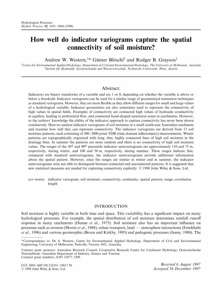
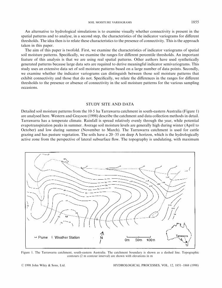
Detailed soil moisture patterns from the 10.5 ha Tarrawarra catchment in south-eastern Australia (Figure 1)are analysed here. Western and Grayson (1998) describe the catchment and data collection methods in detail.Tarrawarra has a temperate climate. Rainfall is spread relatively evenly through the year, while potentialevapotranspiration peaks in summer. Average soil moisture levels are generally high during winter (April toOctober) and low during summer (November to March). The Tarrawarra catchment is used for cattlegrazing and has pasture vegetation. The soils have a 20±35 cm deep A horizon, which is the hydrologicallyactive zone from the perspective of lateral subsurface ¯ow. The topography is undulating, with maximum

Figure 1. The Tarrawarra catchment, south-eastern Australia. The catchment boundary is shown as a dashed line. Topographiccontours (2 m contour interval) are shown with elevations in m



slopes of 14%. There are two distinct drainage lines which join at the runo� measuring ¯ume (Figure 1).These drainage lines become saturated during wet periods.

Thirteen spatial patterns of soil moisture have been collected in this catchment over a period of a year.Each pattern consists of approximately 500 point measurements on a 10 m by 20 m grid, or up to 2000 pointmeasurements with greater spatial detail. Average soil moisture in the top 30 cm of the soil pro®le wasmeasured at each point using time domain re¯ectometry (TDR). The TDR probes were inserted using ahydraulic insertion system mounted on an all-terrain vehicle. Di�erences between gravimetric and TDR soilmoisture measurements collected in the ®eld have a variance of 6.6 (%V/V)2. An analysis of the magnitude ofdi�erent error sources indicates that during normal operating conditions approximately half of this varianceis due to errors in the gravimetric measurements and half to errors in the TDR measurements. Estimates ofnugget variance support this conclusion (Western et al., 1998b). The all-terrain vehicle is ®tted with aposition-®xing system that has a resolution of +0.2 m. Table I provides the dates, antecedent rainfall,number of sample points, mean, variance, coe�cient of variation, and 50th, 75th and 90th percentiles for eachof the data sets used in the analysis. Very detailed information on soil properties and climate data have alsobeen collected which can assist in interpreting the soil moisture patterns (Western and Grayson, 1998).

METHODS OF ANALYSIS

The analysis of the soil moisture patterns consists of four steps. First, indicator values at each measurementsitewere calculated and indicatormapswere plotted. Indicator values were calculated by thresholding the dataat the pth percentile and assigning an indicator value of zero to sites with a soil moisture less than or equal tothe pth percentile, and a value of one to sites with a soil moisture greater than the pth percentile. The indicatormap is then referred to as the pth percentile indicatormap. Indicator maps were calculated for thresholds equalto the 50th, 75th and 90th percentiles. Table I provides these percentiles for each soil moisture pattern.

The second analysis step consisted of calculating indicator semivariograms for each indicator map.Indicator semivariograms were calculated in the same way as standard semivariograms (see, e.g., Isaaks andSrivastava, 1989), except that the indicator values were substituted for the actual soil moisture values. Forone of the occasions (10 November 1996), indicator semivariogram maps were calculated to examine thestatistical anisotropy of the data set. Since the anisotropy did not change between the percentile thresholds,the rest of the analysis was based on omnidirectional indicator semivariograms. These were calculated usingall data pairs separated by lags up to 305 m. This is about half of the maximum separation distance in the

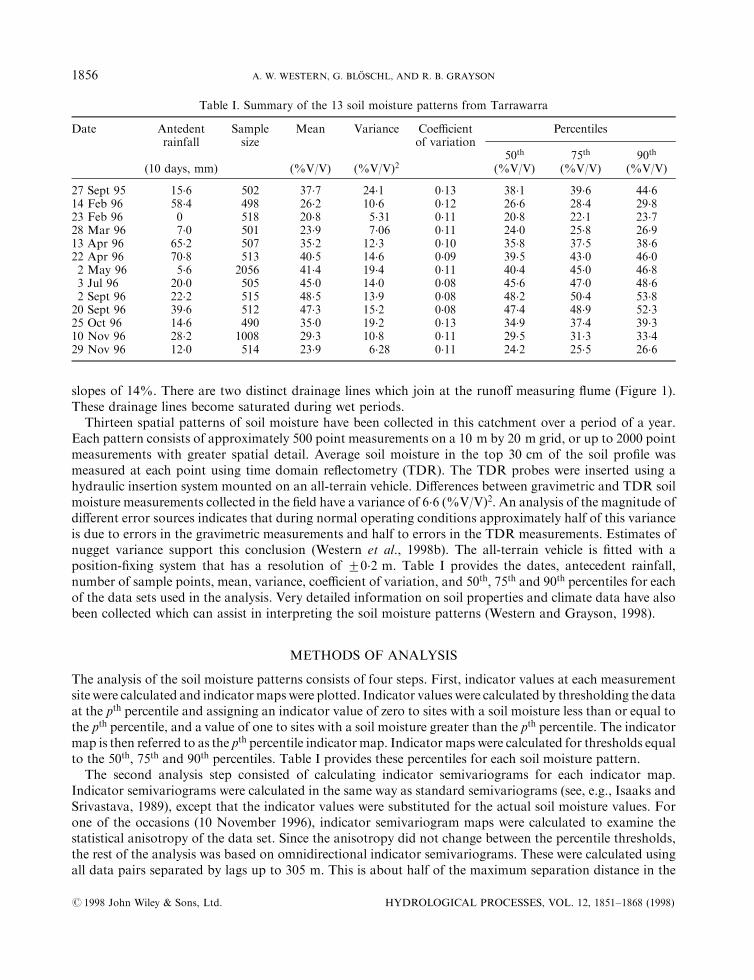
Table I. Summary of the 13 soil moisture patterns from Tarrawarra

Date Antedentrainfall

(10 days, mm)

Samplesize

Mean

(%V/V)

Variance

(%V/V)2

Coe�cientof variation

Percentiles

50th

(%V/V)75th

(%V/V)90th

(%V/V)

27 Sept 95 15.6 502 37.7 24.1 0.13 38.1 39.6 44.614 Feb 96 58.4 498 26.2 10.6 0.12 26.6 28.4 29.823 Feb 96 0 518 20.8 5.31 0.11 20.8 22.1 23.728 Mar 96 7.0 501 23.9 7.06 0.11 24.0 25.8 26.913 Apr 96 65.2 507 35.2 12.3 0.10 35.8 37.5 38.622 Apr 96 70.8 513 40.5 14.6 0.09 39.5 43.0 46.02 May 96 5.6 2056 41.4 19.4 0.11 40.4 45.0 46.83 Jul 96 20.0 505 45.0 14.0 0.08 45.6 47.0 48.62 Sept 96 22.2 515 48.5 13.9 0.08 48.2 50.4 53.820 Sept 96 39.6 512 47.3 15.2 0.08 47.4 48.9 52.325 Oct 96 14.6 490 35.0 19.2 0.13 34.9 37.4 39.310 Nov 96 28.2 1008 29.3 10.8 0.11 29.5 31.3 33.429 Nov 96 12.0 514 23.9 6.28 0.11 24.2 25.5 26.6



catchment. Pairs were grouped into lag `bins' and Equation (1) was used to calculate the indicator semi-variance for that bin. The mean lag of all the pairs in a particular bin was used as the representative lag forthat bin. The sample semivariance, gs(h), is the value of the semivariogram at a given lag, h

gs�h� �1

2N�h�X�i;j��I i ÿ I j�2 �1�

where, N is the number of pairs, Ii and Ij are the indicator values at points i and j, respectively, and thesummation is conducted over all i, j pairs in the lag bin. For indicator semivariograms the range is the mainfeature that contains information about the structure of the spatial ®eld, while the sill is simply a function ofthe percentile at which the data are thresholded. Therefore, the indicator semivariograms were normalized bythe sill such that gn(h)� gs(h)/s

2p, where s

2p � (17 p/100)p/100 is the variance of the indicator values at the pth

percentile. The sill of the normalized indicator variograms is equal to 1. The range of the normalizedindicator variograms is equal to the range of the original indicator variograms. The di�erences in range forthe di�erent thresholds are of most interest.

The third analysis step involved calculating ranges for each sample indicator semivariogram. Threeapproaches were used to calculate the ranges. The ®rst approach was to ®t an exponential semivariogrammodel to the sample semivariogram and to use the range parameter from the ®tted semivariograms asestimates of the range

ge�h� �s20s2p� 1 ÿ s20

s2p

!�1 ÿ e

ÿh=l� �2�

In Equation (2), l is the correlation length, and the practical range is 3l. s20/s2p is the normalized nugget. The

second approach was similar but used a spherical variogram model

gsp�h� �s20s2p� 1 ÿ s20

s2p

!1�5 h

aÿ 0�5 h

a

� �3" #

h5 a �3a�

gsp�h� � 1 h5 a �3b�

In Equation (3), a is the range. The third approach consisted of estimating the range directly from the sampleindicator semivariograms by visual inspection.

The last analysis step was to compare the estimated ranges for the di�erent thresholds. For a multi-Gaussian random ®eld, the ratio of the ranges at two percentile thresholds is uniquely de®ned by thepercentile values and the shape of the (traditional) semivariogram. Western et al. (1998b) showed that the(traditional) semivariograms of the Tarrawarra soil moisture data set are approximately exponential with anugget. For this type of variogram, the ratio of the ranges at the 90th and the 50th percentiles is about 0.8 ifthe ®eld is multi-Gaussian (Deutsch and Journel, 1992, equation V.20, p. 139). Estimated values of the ratiodi�erent from 0.8 indicate that the ®eld is not multi-Gaussian. If the indicator approach is able to captureconnectivity one would expect signi®cantly di�erent ratios for connected and not connected soil moisturepatterns.

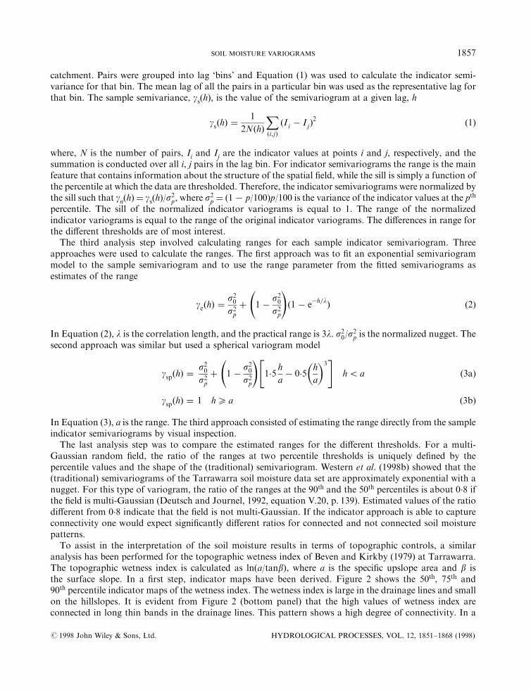
To assist in the interpretation of the soil moisture results in terms of topographic controls, a similaranalysis has been performed for the topographic wetness index of Beven and Kirkby (1979) at Tarrawarra.The topographic wetness index is calculated as ln(a/tanb), where a is the speci®c upslope area and b isthe surface slope. In a ®rst step, indicator maps have been derived. Figure 2 shows the 50th, 75th and90th percentile indicator maps of the wetness index. The wetness index is large in the drainage lines and smallon the hillslopes. It is evident from Figure 2 (bottom panel) that the high values of wetness index areconnected in long thin bands in the drainage lines. This pattern shows a high degree of connectivity. In a



second step, indicator semivariograms were derived from these indicator plots. Figure 3 shows 50th, 75th and90th percentile indicator semivariograms for the wetness index. Here, the range for the 90th percentileindicator semivariogram is about two-thirds of the range of the 50th percentile indicator semivariogram. Thisis signi®cantly lower than the theoretical value of 0.8 which indicates that the wetness index spatial ®eld is notmulti-Gaussian. The ®eld is less spatially continuous (the bands are narrower) at high wetness index valuesthan at the median wetness index value and the di�erence is larger than would be expected for a multi-Gaussian ®eld. Because of this, there is more spatial structure in the wetness index ®eld than can be capturedusing a traditional semivariogram. If the soil moisture ®eld is topographically organized, similar indicatorplots and similar indicator semivariograms can be expected for the soil moisture ®eld.

RESULTS

Indicator maps

Here the spatial pattern of soil moisture is examined using indicator maps. Figures 4±6 show 50th, 75th and90th percentile indicator maps, respectively, for soil moisture in the Tarrawarra catchment on 12 di�erentoccasions. When comparing the 50th and 90th percentile indicator maps, the most striking di�erence is thelow proportion of high moisture (black) cells in the 90th percentile map. Obviously this is due to the highermoisture threshold, which is exceeded only by 10% of the cells. The 90th percentile map shows the core or thewettest part of the wet areas in the 50th percentile map. Two other comparisons are more hydrologicallyinteresting.

The ®rst is a comparison of the characteristics of the soil moisture patterns during di�erent seasons. Thiscan be illustrated using the 75th percentiles in Figure 5. In the patterns from 14 and 23 February, and28 March 1996 there are black patches spread across the catchment in a relatively random manner. Whilethere is some tendency for high moisture measurements to group together, the high moisture patches are not

Figure 2. Indicator maps the topographic wetness index in the Tarrawarra catchment. Top 50th, middle 75th and bottom 90th percentile.The raster grid is 20 m by 10 m. Black cells have wetness index values greater than the threshold and grey cells have wetness index

values less than or equal to the threshold



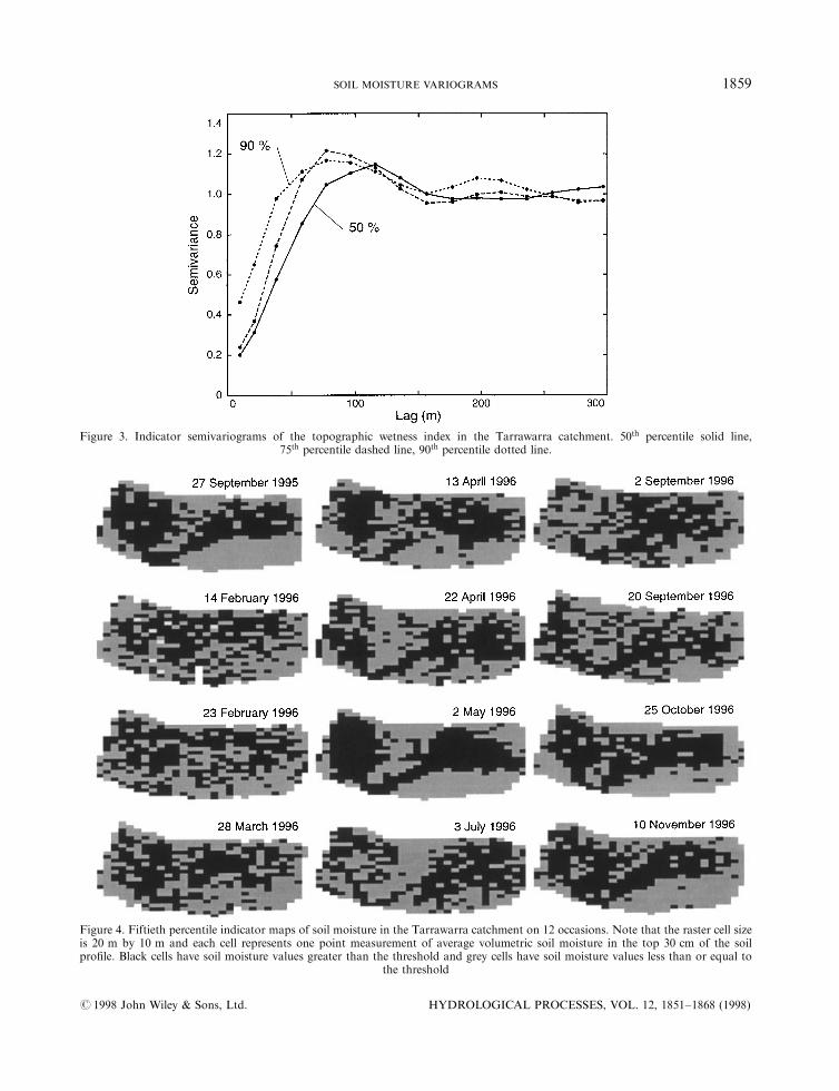
Figure 3. Indicator semivariograms of the topographic wetness index in the Tarrawarra catchment. 50th percentile solid line,75th percentile dashed line, 90th percentile dotted line.

Figure 4. Fiftieth percentile indicator maps of soil moisture in the Tarrawarra catchment on 12 occasions. Note that the raster cell sizeis 20 m by 10 m and each cell represents one point measurement of average volumetric soil moisture in the top 30 cm of the soilpro®le. Black cells have soil moisture values greater than the threshold and grey cells have soil moisture values less than or equal to

the threshold



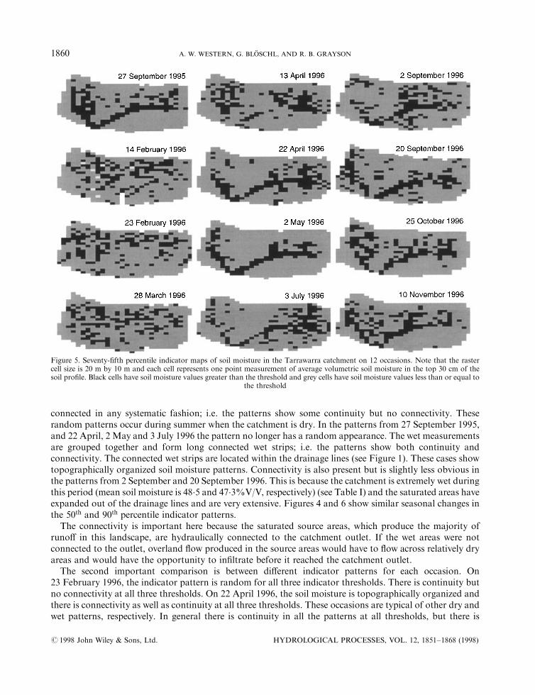
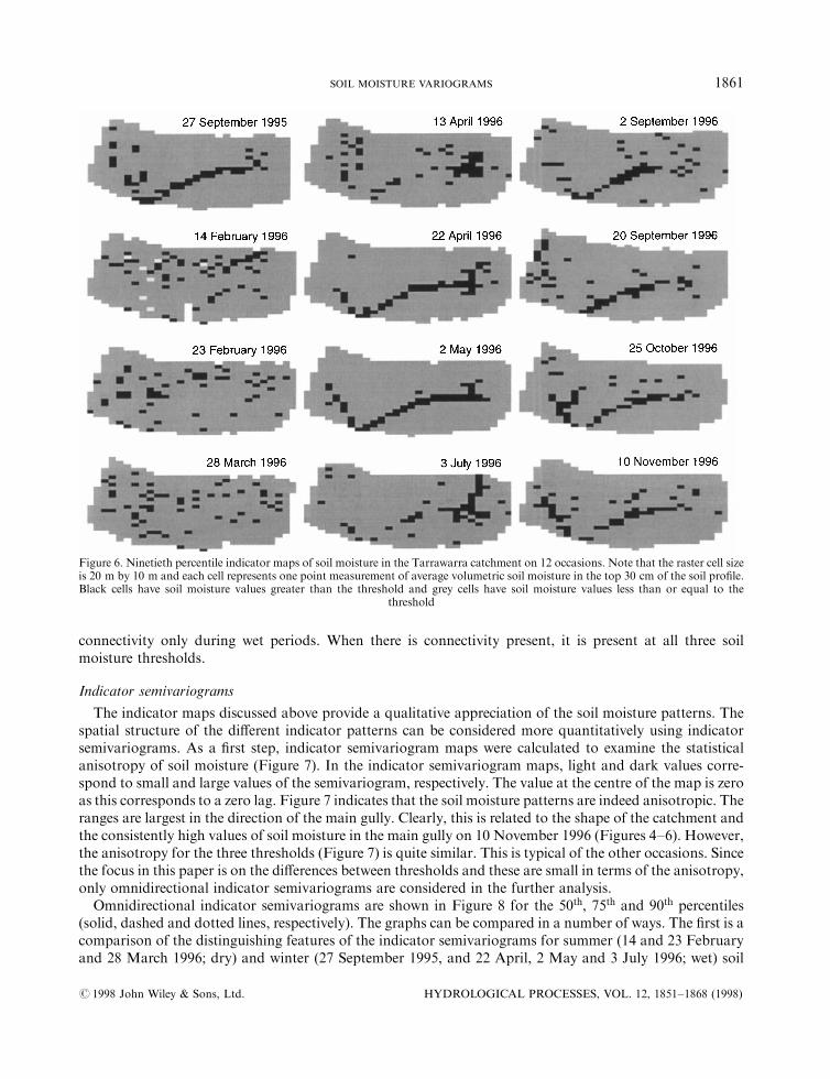
connected in any systematic fashion; i.e. the patterns show some continuity but no connectivity. Theserandom patterns occur during summer when the catchment is dry. In the patterns from 27 September 1995,and 22 April, 2 May and 3 July 1996 the pattern no longer has a random appearance. The wet measurementsare grouped together and form long connected wet strips; i.e. the patterns show both continuity andconnectivity. The connected wet strips are located within the drainage lines (see Figure 1). These cases showtopographically organized soil moisture patterns. Connectivity is also present but is slightly less obvious inthe patterns from 2 September and 20 September 1996. This is because the catchment is extremely wet duringthis period (mean soil moisture is 48.5 and 47.3%V/V, respectively) (see Table I) and the saturated areas haveexpanded out of the drainage lines and are very extensive. Figures 4 and 6 show similar seasonal changes inthe 50th and 90th percentile indicator patterns.

The connectivity is important here because the saturated source areas, which produce the majority ofruno� in this landscape, are hydraulically connected to the catchment outlet. If the wet areas were notconnected to the outlet, overland ¯ow produced in the source areas would have to ¯ow across relatively dryareas and would have the opportunity to in®ltrate before it reached the catchment outlet.

The second important comparison is between di�erent indicator patterns for each occasion. On23 February 1996, the indicator pattern is random for all three indicator thresholds. There is continuity butno connectivity at all three thresholds. On 22 April 1996, the soil moisture is topographically organized andthere is connectivity as well as continuity at all three thresholds. These occasions are typical of other dry andwet patterns, respectively. In general there is continuity in all the patterns at all thresholds, but there is

Figure 5. Seventy-®fth percentile indicator maps of soil moisture in the Tarrawarra catchment on 12 occasions. Note that the rastercell size is 20 m by 10 m and each cell represents one point measurement of average volumetric soil moisture in the top 30 cm of thesoil pro®le. Black cells have soil moisture values greater than the threshold and grey cells have soil moisture values less than or equal to

the threshold



connectivity only during wet periods. When there is connectivity present, it is present at all three soilmoisture thresholds.

Indicator semivariograms

The indicator maps discussed above provide a qualitative appreciation of the soil moisture patterns. Thespatial structure of the di�erent indicator patterns can be considered more quantitatively using indicatorsemivariograms. As a ®rst step, indicator semivariogram maps were calculated to examine the statisticalanisotropy of soil moisture (Figure 7). In the indicator semivariogram maps, light and dark values corre-spond to small and large values of the semivariogram, respectively. The value at the centre of the map is zeroas this corresponds to a zero lag. Figure 7 indicates that the soil moisture patterns are indeed anisotropic. Theranges are largest in the direction of the main gully. Clearly, this is related to the shape of the catchment andthe consistently high values of soil moisture in the main gully on 10 November 1996 (Figures 4±6). However,the anisotropy for the three thresholds (Figure 7) is quite similar. This is typical of the other occasions. Sincethe focus in this paper is on the di�erences between thresholds and these are small in terms of the anisotropy,only omnidirectional indicator semivariograms are considered in the further analysis.

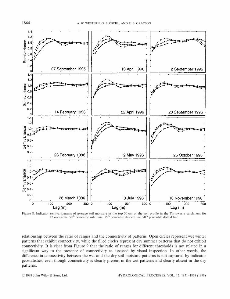
Omnidirectional indicator semivariograms are shown in Figure 8 for the 50th, 75th and 90th percentiles(solid, dashed and dotted lines, respectively). The graphs can be compared in a number of ways. The ®rst is acomparison of the distinguishing features of the indicator semivariograms for summer (14 and 23 Februaryand 28 March 1996; dry) and winter (27 September 1995, and 22 April, 2 May and 3 July 1996; wet) soil

Figure 6. Ninetieth percentile indicator maps of soil moisture in the Tarrawarra catchment on 12 occasions. Note that the raster cell sizeis 20 m by 10 m and each cell represents one point measurement of average volumetric soil moisture in the top 30 cm of the soil pro®le.Black cells have soil moisture values greater than the threshold and grey cells have soil moisture values less than or equal to the

threshold



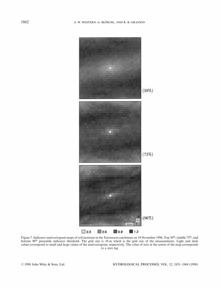
Figure 7. Indicator semivariogram maps of soil moisture in the Tarrawarra catchment on 10 November 1996. Top 50th, middle 75th, andbottom 90th percentile indicator threshold. The grid size is 10 m which is the grid size of the measurements. Light and darkvalues correspond to small and large values of the semivariogram, respectively. The value of zero at the centre of the map corresponds

to a zero lag



moisture patterns. During summer the normalized nugget is larger than during winter. This is related to themeasurement error and the variance of the soil moisture pattern. When the ratio of the measurement error tothe variance of the soil moisture is high, the normalized nugget is high. In summer the variance of the soilmoisture is low while during the winter the variance of the soil moisture is high. Since the measurement erroris relatively constant, there is a high normalized nugget in summer and a low normalized nugget in winter.

Another feature distinguishing the indicator semivariograms for the summer (dry) and winter (wet) soilmoisture patterns is the periodicity that appears in the indicator semivariograms, particularly for the 90th

percentile, during wet periods. This is related to the organization of the soil moisture pattern, speci®cally thewet drainage lines. This organization introduces a periodic component into the soil moisture pattern whichappears as periodicity in the semivariogram. However, this is likely to be an artefact of having a singlecatchment and is probably not a characteristic of the landscape as a whole. We would expect it to disappear ifmultiple catchments were studied. Neither the nugget nor the periodicity are features of the indicatorsemivariograms that would be useful for distinguishing between the connected and unconnected (i.e. the wetand the dry) patterns in a general way.

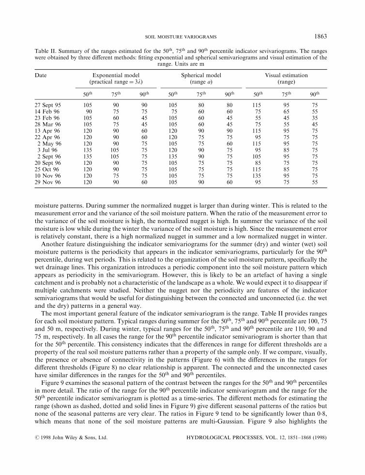
The most important general feature of the indicator semivariogram is the range. Table II provides rangesfor each soil moisture pattern. Typical ranges during summer for the 50th, 75th and 90th percentile are 100, 75and 50 m, respectively. During winter, typical ranges for the 50th, 75th and 90th percentile are 110, 90 and75 m, respectively. In all cases the range for the 90th percentile indicator semivariogram is shorter than thatfor the 50th percentile. This consistency indicates that the di�erences in range for di�erent thresholds are aproperty of the real soil moisture patterns rather than a property of the sample only. If we compare, visually,the presence or absence of connectivity in the patterns (Figure 6) with the di�erences in the ranges fordi�erent thresholds (Figure 8) no clear relationship is apparent. The connected and the unconnected caseshave similar di�erences in the ranges for the 50th and 90th percentiles.

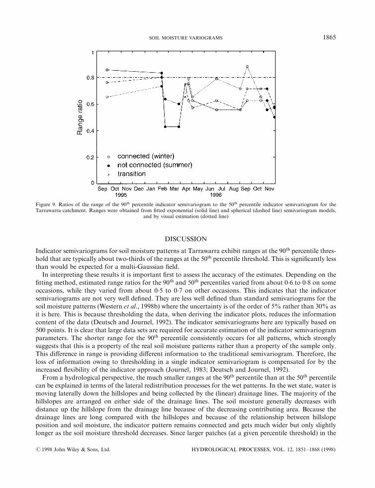
Figure 9 examines the seasonal pattern of the contrast between the ranges for the 50th and 90th percentilesin more detail. The ratio of the range for the 90th percentile indicator semivariogram and the range for the50th percentile indicator semivariogram is plotted as a time-series. The di�erent methods for estimating therange (shown as dashed, dotted and solid lines in Figure 9) give di�erent seasonal patterns of the ratios butnone of the seasonal patterns are very clear. The ratios in Figure 9 tend to be signi®cantly lower than 0.8,which means that none of the soil moisture patterns are multi-Gaussian. Figure 9 also highlights the

Table II. Summary of the ranges estimated for the 50th, 75th and 90th percentile indicator sevivariograms. The rangeswere obtained by three di�erent methods: ®tting exponential and spherical semivariograms and visual estimation of the

range. Units are m

Date Exponential model(practical range� 3l)

Spherical model(range a)

Visual estimation(range)

50th 75th 90th 50th 75th 90th 50th 75th 90th

27 Sept 95 105 90 90 105 80 80 115 95 7514 Feb 96 90 75 75 75 60 60 75 65 5523 Feb 96 105 60 45 105 60 45 55 45 3528 Mar 96 105 75 45 105 60 45 75 55 4513 Apr 96 120 90 60 120 90 90 115 95 7522 Apr 96 120 90 60 120 75 75 95 75 752 May 96 120 90 75 105 75 60 115 95 753 Jul 96 135 105 75 120 90 75 95 85 752 Sept 96 135 105 75 135 90 75 105 95 7520 Sept 96 120 90 75 105 75 75 85 75 7525 Oct 96 120 90 75 105 75 75 115 85 7510 Nov 96 120 75 75 105 75 75 135 95 7529 Nov 96 120 90 60 105 90 60 95 75 55



relationship between the ratio of ranges and the connectivity of patterns. Open circles represent wet winterpatterns that exhibit connectivity, while the ®lled circles represent dry summer patterns that do not exhibitconnectivity. It is clear from Figure 9 that the ratio of ranges for di�erent thresholds is not related in asigni®cant way to the presence of connectivity as assessed by visual inspection. In other words, thedi�erence in connectivity between the wet and the dry soil moisture patterns is not captured by indicatorgeostatistics, even though connectivity is clearly present in the wet patterns and clearly absent in the drypatterns.

Figure 8. Indicator semivariograms of average soil moisture in the top 30 cm of the soil pro®le in the Tarrawarra catchment for12 occasions. 50th percentile solid line, 75th percentile dashed line, 90th percentile dotted line



DISCUSSION

Indicator semivariograms for soil moisture patterns at Tarrawarra exhibit ranges at the 90th percentile thres-hold that are typically about two-thirds of the ranges at the 50th percentile threshold. This is signi®cantly lessthan would be expected for a multi-Gaussian ®eld.

In interpreting these results it is important ®rst to assess the accuracy of the estimates. Depending on the®tting method, estimated range ratios for the 90th and 50th percentiles varied from about 0.6 to 0.8 on someoccasions, while they varied from about 0.5 to 0.7 on other occasions. This indicates that the indicatorsemivariograms are not very well de®ned. They are less well de®ned than standard semivariograms for thesoil moisture patterns (Western et al., 1998b) where the uncertainty is of the order of 5% rather than 30% asit is here. This is because thresholding the data, when deriving the indicator plots, reduces the informationcontent of the data (Deutsch and Journel, 1992). The indicator semivariograms here are typically based on500 points. It is clear that large data sets are required for accurate estimation of the indicator semivariogramparameters. The shorter range for the 90th percentile consistently occurs for all patterns, which stronglysuggests that this is a property of the real soil moisture patterns rather than a property of the sample only.This di�erence in range is providing di�erent information to the traditional semivariogram. Therefore, theloss of information owing to thresholding in a single indicator semivariogram is compensated for by theincreased ¯exibility of the indicator approach (Journel, 1983; Deutsch and Journel, 1992).

From a hydrological perspective, the much smaller ranges at the 90th percentile than at the 50th percentilecan be explained in terms of the lateral redistribution processes for the wet patterns. In the wet state, water ismoving laterally down the hillslopes and being collected by the (linear) drainage lines. The majority of thehillslopes are arranged on either side of the drainage lines. The soil moisture generally decreases withdistance up the hillslope from the drainage line because of the decreasing contributing area. Because thedrainage lines are long compared with the hillslopes and because of the relationship between hillslopeposition and soil moisture, the indicator pattern remains connected and gets much wider but only slightlylonger as the soil moisture threshold decreases. Since larger patches (at a given percentile threshold) in the

Figure 9. Ratios of the range of the 90th percentile indicator semivariogram to the 50th percentile indicator semivariogram for theTarrawarra catchment. Ranges were obtained from ®tted exponential (solid line) and spherical (dashed line) semivariogram models,

and by visual estimation (dotted line)



indicator plot relate to longer ranges, the range increases as the threshold decreases. This interpretation issupported by the indicator plots and the indicator semivariograms of the wetness index (Figures 2 and 3).Both the indicator plots and the indicator semivariograms of the wetness index are similar to those of soilmoisture for the wet (winter) conditions. The wetness index can be thought of as a limiting case of a spatialpattern that is strongly controlled by topography. Indeed, Figure 2 very clearly illustrates the increasingwidth of the indicator pattern as the threshold decreases from the bottom to the top panel. This change inwidth translates into a change in the range of the indicator semivariograms of the wetness index fromabout 60 m at the 90th percentile to about 100 m at the 50th percentile (Figure 3). In other words, the largedi�erences in range for the wet soil moisture patterns can be interpreted in terms of the strong topographiccontrol.

For the dry case, there is no topographic control but the ranges at the 90th percentile are still signi®cantlysmaller than those at the 50th percentile. There is no clear explanation for this result. It is possibly related tosoil variations, particularly zones of di�erent soil types, to a slight in¯uence of aspect and slope on evapo-transpiration (owing to di�erent radiation inputs) or to some small patches of local lateral redistribution.

It is interesting to note that the change in range with changing threshold for the soil moisture patterns isopposite to the characteristics found for the conductivity in aquifers. In the aquifer case, often, the ranges forthe highest percentiles are signi®cantly larger than those for the lower percentiles (Scheibe, 1993; BloÈ schl;1996; GoÂ mez-HernaÂ ndez and Wen, 1997). This is not a contradiction, as the processes giving rise to thespatial patterns are vastly di�erent in the soil moisture and the aquifer cases.

While there is a large di�erence in range for di�erent thresholds, this di�erence was present for bothconnected and unconnected patterns. Therewas no clear dependence of the di�erence in range on the presenceor absence of connectivity. Therefore it must be concluded that the indicator semivariograms did not capturethe connectivity. This is opposite to what some authors have suggested in the literature. To shed more lighton this question we need to consider two things. First, what does the indicator semivariogram capture andhow is this related to connectivity, and secondly, what are the features of our patterns that change withthreshold?

Standard semivariograms are a measure of spatial continuity in general. Indicator semivariograms are ameasure of spatial continuity at a speci®c threshold. Multiple indicator semivariograms capture spatial con-tinuity at multiple thresholds and can thus be used to capture di�erences in continuity at di�erent thresholds,an important feature of many natural spatial patterns. Depending on the nature of the spatial patterns,connectivity may or may not be associated with di�erences in continuity at di�erent thresholds. However,because continuity and connectivity are two distinct properties of a spatial pattern, there are many possiblecombinations of connectivity and continuity at di�erent thresholds.

Consider ®rst the case of a multi-Gaussian random ®eld such as would be simulated by the turning bandsmethods (Mantoglou and Wilson, 1981). This type of ®eld has no connectivity (rounded shapes on a map)and the continuity (i.e. the range) is equal for all thresholds. The second case is the summer (dry) patternsanalysed in this study. These patterns have no connectivity and di�erent continuity at the 50th, 75th and 90th

percentiles. In an indicator plot, smaller continuity at the 90th percentile translates into a larger number ofsmaller patches at the 90th percentile as compared with a multi-Gaussian ®eld. These patches tend to beisolated and not connected with each other. The third case is the winter (wet) patterns. These patterns haveconnectivity at all percentile thresholds and di�erent continuity at the 50th, 75th and 90th percentiles. Thepresence of connectivity at all thresholds is related to the signi®cant topographically routed lateral ¯ow alongboth subsurface and surface ¯ow paths during the wet conditions in winter. Because there are lateralredistribution processes operating everywhere and because these processes, along with the convergence ofcatchments in general, have an inherent tendency to create connectivity, there is connectivity at all thres-holds. A fourth possible case is an aquifer with high conductivity ¯ow paths which has connectivity at thehigh percentile thresholds only and di�erent continuity at the di�erent percentiles. The processes leading toconnectivity can include ¯uvial sedimentary processes, fracturing and faulting (SaÂ nchez-Vila et al., 1996;Anderson, 1997). These are not processes that operate at all points in the ®eld at the same time and therefore



it would not be expected that they would lead to connectivity at all thresholds. The same processes may giverise to di�erences in continuity at the di�erent percentiles. In other words, this is an example wheredi�erences in connectivity are likely to be associated with di�erences in continuity at di�erent thresholds.

It is clear that for some spatial hydrological patterns, connectivity may be associated with di�erences incontinuity at di�erent thresholds. However, this depends on the nature of the spatial process and there doesnot appear to be a universal correspondence.

CONCLUSIONS

Indicator semivariograms of soil moisture patterns at Tarrawarra have been examined. Indicator semi-variogrammaps indicate that there is substantial anisotropy with the larger ranges in the direction of themaingully. However, this anisotropy is present for all indicator thresholds. Omnidirectional indicator semi-variograms have been analysed in terms of their ranges. Typical ranges during summer for the 50th, 75th and90th percentile are 100, 75 and 50 m, respectively. Typical ranges during winter for the 50th, 75th and90th percentile are 110, 90 and 75 m, respectively. In all cases the range for the 90th percentile indicatorsemivariogram is shorter than that for the 50th percentile. This consistency indicates that the di�erences inrange for di�erent thresholds are a property of the real soil moisture patterns rather than a property of thesample only. The ranges are similar to those of the indicator semivariograms for the topographic wetnessindex of Beven and Kirkby (1979). For the wetness index, the ranges for the 50th, 75th and 90th percentile areabout 100, 80 and 60 m, respectively. Since, for the soil moisture patterns, the ratio of the ranges at the 90th

percentile and the ranges at the 50th percentile is always smaller than its theoretical value of 0.8 for a multi-Gaussian ®eld, none of the soil moisture patterns are multi-Gaussian. Because of this, the indicatorsemivariograms provide additional information about the spatial pattern, compared with standard semi-variograms. Using this information may be an improvement over assuming multi-Gaussianity, especially inthe summer (dry) case, where no connectivity is present. For example, sequential indicator simulation(Deutsch and Journel, 1992), instead of multi-Gaussian simulation methods such as the turning bandsmethod, could be used to simulate the spatial pattern of soil moisture for input into a physically basedrainfall±runo� model.

This study also examined how well indicator semivariograms can capture the spatial connectivity of soilmoisture. The winter (wet) patterns exhibited a large degree of connectivity, while the summer (dry) patternsdid not exhibit any connectivity. However, the indicator semivariograms for the winter and the summerpatterns are similar in terms of their range. Speci®cally, the ratio of the ranges at the 90th and 50th percentilesis on the order of 0.6 to 0.7 for both the winter and the summer patterns. This ratio is the key property thatcan capture spatial structure beyond that of a traditional semivariogram. Since there is no clear dependenceof the ratio of the ranges on the presence (winter patterns) or absence (summer patterns) of connectivity, itmust be concluded that the indicator semivariograms did not capture the connectivity. Multiple indicatorsemivariograms capture spatial continuity at multiple thresholds and can thus be used to capture di�erencesin continuity at di�erent thresholds. Depending on the nature of the spatial patterns, connectivity may ormay not be associated with di�erences in continuity at di�erent thresholds.

There are a number of possible approaches to consider connectivity more explicitly. These may be moreappropriate for generating spatial patterns of soil moisture for the wet (winter) case than indicator-basedapproaches. One approach is to consider topograph explicitly, either as a covariate or by using coordinatesystems de®ned by topographic contours and ¯ow lines. Another possible approach is to use explicitconnectivity measures (see Allard, 1994). Work along these lines will be reported in the near future.

ACKNOWLEDGEMENTS

The Tarrawarra catchment is owned by the Cistercian Monks (Tarrawarra) who have provided free access totheir land and willing cooperation throughout this project. Funding for the above work was provided by the



Australian Research Council (project A39531077), the Cooperative Research Centre for CatchmentHydrology, the Oesterreichische Nationalbank, Vienna (project 5309), and the Australian Department ofIndustry, Science and Tourism, International Science and Technology programme.

REFERENCES

Allard, D. 1994. `Simulating a geological lithofacies with respect to connectivity information using the truncated Gaussian model',in Armstrong, M. and Dowd, P. A. (eds), Geostatistical Simulations. Kluwer Academic Publishers, Dordrecht, The Netherlands.pp. 197±211.

Anderson, M. P. 1997. `Characterization of geological heterogeneity', in Dagan, G. and Neuman, S. P. (eds), Subsurface Flow andTransport. Cambridge University Press, Cambridge. pp. 23±43.

ASCE Task Committee on Geostatistical Techniques in Geohydrology of the Ground Water hydrology Committee of the ASCEHydraulics Division, 1990. `Review of geostatistics in geohydrology. I: Basic concepts', J. Hydraul. Engng, 116, 612±632.

Beven, K. J. and Kirby, M. J. 1979. À physically-based variable contributing area model of basin hydrology', Hydrol. Sci. B., 24, 43±69.

Beven, K. and Kirkby, M. J. (eds) 1993. Channel Network Hydrology. Wiley, Chichester.BloÈ schl, G. 1996. `Scale and scaling in hydrology'. Habilitationsschrift. Wiener Mitteilungen, Wasser-Abwasser-GewaÈsser, vol. 132.

Technical University of Vienna, Vienna.Desbarats, A. J. and Srivistava, R. M. 1991. `Geostatistical characterisation of groundwater ¯ow parameters in a simulated aquifer',

Wat. Resour. Res., 27, 687±698.Deutsch, C. V. and Journel, A. G. 1992. GSLIB Geostatistical Software Library and User's Guide. Oxford University Press, New York.

340 pp.Dunne, T., Moore, T. R., and Taylor, C. H. 1975 `Recognition and prediction of runo�-producing zones in humid regions',Hydrol. Sci.

B, 20, 305±327.Entekhabi, D., Rodriguez-Iturbe, I., and Castelli, F. 1996. `Mutual interaction of soil moisture state and atmospheric processes',

J. Hydrol., 184, 3±17.GoÂ mez-HernaÂ ndez, J. J. and Wen, X.-H. 1997. `To be or not to be multi-Gaussian? A re¯ection on stochastic hydrogeology', Adv. Wat.

Resour., 21, 47±61.Grayson, R. B., BloÈ schl, G., and Moore, I. D. 1995. `Distributed parameter hydrologic modelling using vector elevation data:

Thales and TAPES-C', in Singh, V. P. (ed.), Computer Models of Watershed Hydrology. Water Resources Pub., Highlands Ranch,Colorardo. pp. 669±695.

Guardiano, F. B. and Srivastava, R. M. 1993. `Multivariate geostatistics: beyond bivariate moments', in Soares, A. (ed.), GeostatisticsTroÂia '92. Kluwer Academic Publishers, Dordrecht, The Netherlands. pp. 133±144.

Isaaks, E. H. and Srivastava, R. M. 1989. An Introduction to Applied Geostatistics. Oxford University Press, New York. 561 pp.Jackson, T. J. and Le Vine, D. E. 1996. `Mapping surface soil moisture using an aircraft-based passive microwave instrument: algorithm

and example', J. Hydrol., 184, 57±84.Jenny, H. 1980. The Soil Resource. Springer-Verlag, New York. 377 pp.Journel, A. G. 1983. `Nonparametric estimation of spatial distributions', Math. Geol., 15, 445±468.Journel, A. G. 1986. `Geostatistics: models and tools for the Earth Sciences', Math. Geol., 18, 119±140.Journel, A. G. 1993. `Geostatistics: roadblocks and challenges', in Soares, A. (ed.),Geostatistics TroÂia '92. Kluwer Academic Publishers,

Dordrecht, The Netherlands. pp. 213±224.Journel, A. G and Alabert, F. 1989. `Non-Gaussian data expansion in the Earth Sciences', Terra Nova, 1, 123±134.Journel, A. G. and Deutsch, C. V. 1993. Èntropy and spatial disorder', Math. Geol., 25, 329±355.Journel, A. G. and Huijbregts, C. J. 1978. Mining Geostatistics. Academic Press, London. 600 pp.Koltermann, C. E. and Gorelick, S. M. 1996. `Heterogeneity in sedimentary deposits: a review of structure-imitating, process-imitating

and descriptive approaches', Wat. Resour. Res., 32, 2617±2658.Mantoglou, A. and Wilson, J. L. 1981. `Simulation of random ®elds with the turning bands method', Department of Civil Engineering,

Massachusetts Institute of Technology, report no. 264. MIT, Cambridge, Massachusetts.Moore, I. D., Burch, G. J., and Mackenzie, D. H. 1988. `Topographic e�ects on the distribution of surface soil water and the location of

ephemeral gullies', Trans. Am. Soc. Agric. Eng., 31, 1098±1107.Rubin, Y. and Journel, A. G. 1991. `Simulation of non-Gaussian space random functions for modelling transport in groundwater',

Wat. Resour. Res., 27, 1711±1721.SaÂ nchez-Vila, X., Carrera, J., and Girardi, J. P. 1996. `Scale e�ects in transmissivity', J. Hydrol., 183, 1±22.Scheibe, T. D. 1993. `Characterization of the spatial structuring of natural porous media and its impacts on subsurface ¯ow and

transport', PhD Thesis, Stanford University, Palo Alto.Western, A. W. and Grayson, R. B. 1998. `The Tarrawarra data set: soil moisture patterns, soil characteristics and hydrological ¯ux

measurements', Wat. Resour. Res., in press.Western, A. W., Grayson, R. B., BloÈ schl, G., Willgoose, G. R., and McMahon, T. A. 1998a. Òbserved spatial organization of soil

moisture and relation to terrain indices', Wat. Resour. Res., submitted.Western, A. W., BloÈ schl, G., and Grayson, R. B. 1998b. `Geostatistical characterisation of soil moisture patterns in the Tarrawarra

Catchment', J. Hydrol., in press.



western, a. w., g. blöschl and r. b. grayson (1998) how well do indicator variograms capture the...

Documents