wave effect in gravitational lensing by the ellis wormhole
TRANSCRIPT

arX
iv:1
302.
7170
v2 [
gr-q
c] 6
Mar
201
3
Yukawa Institute for Theoretical Physics
Kyoto University
Department of Physics
Rikkyo University
YITP-13-15
RUP-13-3
Wave Effect in Gravitational Lensing by the Ellis Wormhole
Chul-Moon Yoo,1, ∗ Tomohiro Harada,2 and Naoki Tsukamoto2
1 Yukawa Institute for Theoretical Physics,
Kyoto University Kyoto 606-8502, Japan
2 Department of Physics, Rikkyo University, Tokyo 171-8501, Japan
We propose the use of modulated spectra of astronomical sources due to gravita-
tional lensing to probe Ellis wormholes. The modulation factor due to gravitational
lensing by the Ellis wormhole is calculated. Within the geometrical optics approx-
imation, the normal point mass lens and the Ellis wormhole are indistinguishable
unless we know the source’s unlensed luminosity. This degeneracy is resolved with
the significant wave effect in the low frequency domain if we take the deviation from
the geometrical optics into account. We can roughly estimate the upper bound for
the number density of Ellis wormholes as n . 10−9AU−3 with throat radius a ∼ 1cm
from the existing femto-lensing analysis for compact objects.
∗Electronic address: [email protected]

2
I. INTRODUCTION
In a variety of cosmological models based on fundamental theory, exotic astrophysical
objects which have not been observed are often predicted. Conversely, an observational
evidence for an exotic object would stimulate creative theoretical discussions. Probing these
exotic objects and detecting them will give us significant progress of research in fundamental
physics. Even if we cannot detect it, giving a constraint on the abundance of the exotic
objects is one of powerful means of investigating the nature of our universe.
Generally, the interaction between such unobserved exotic objects and well known matters
is very weak or not well established. Thus, only the gravitational interaction would cause
reliable observational phenomena. One of the most direct measurements of gravitational
effects of an exotic object is gravitational lensing. For instance, massive compact halo
objects are probed by using micro-lensing[1–3]. Cosmic strings are also targets for probing
by using gravitational lensing phenomena[4–12]. In this paper, we propose a way to probe
Ellis wormholes[13] by using lensed spectra of astronomical sources.
The Ellis wormhole was first introduced by Ellis as a spherically symmetric solution of
Einstein equations with a ghost massless scalar field. The dynamical stability of the Ellis
wormhole is discussed in Ref. [14] and the possible source to support the Ellis geometry
was proposed in Ref. [15]. Gravitational lensing by the Ellis wormhole was studied in
Refs. [16, 17] and recently revisited by several authors[18, 19]. So far, it has been suggested
that Ellis wormholes can be probed by using light curves of gamma-ray bursts [20], micro-
lensing [21–23] (see also Refs. [24, 25]) and imaging observations [26, 27], while our proposal
is the use of spectroscopic observations to probe Ellis wormholes.
In order to fully investigate the lensed spectrum of a point source, the wave effect in
gravitational lensing must be taken into account. The wave effect for the point mass lens
is discussed in Refs. [28, 29]. Wave effects in gravitational lensing by the rotating massive
object[30], binary system[31], singular isothermal sphere[32] and the cosmic string[33, 34]
have been considered. In Sec. II, we calculate the amplification factor of gravitational lensing
by the Ellis wormhole taking the wave effect into account. The geometrical optics limit is
analytically presented in Sec. III. The difference in the amplification factor between the
point mass lens and the Ellis wormhole lens is discussed in Sec. IV based on observables.
In Sec. V, possible observations to probe Ellis wormholes are listed. Sec. VI is devoted to a
summary.
In this paper, we use the geometrized units in which the speed of light and Newton’s
gravitational constant are both unity.
II. A DERIVATION OF THE LENSED WAVE FORM
The line element in the Ellis wormhole spacetime can be written by the following isotropic
form:
ds2 = −dt2 +
(
1 +a2
R2
)2(
dR2 +R2dΩ2)
, (1)

3
where R = a corresponds to the throat and we simply call a the throat radius in this paper.1
Assuming the thin lens approximation is valid, we consider the wormhole lens system
shown in Fig. 1. We use the position vector ~X = (X, Y, Z) in the flat space. Then, the
FIG. 1: Lens system with thin lens approximation. S, L, and O represent the source, lens, and
observer positions, respectively. The path SAB is a ray trajectory which is specified with the vector
~ξ on the lens plane ΣA. B′ is the intersection of the line AO and the plane ΣB. ~ξ′ is the position
vector of the point B on the plane ΣB.
coordinate R is given by R = | ~X − ~XL|, where | ~XL| is the lens position. We set Z-axis as
the perpendicular direction to the lens plane and the source plane. DS, DL, and DLS denote
the distances from the observer plane to the source plane, from the observer plane to the
lens plane, and from the lens plane to the source plane, respectively.
In the geometrical optics limit, we consider light rays emanated from the source. The
vector ~ξ on the lens plane ΣA in Fig. 1 specifies the light ray which is deflected once at~X = ~XL + ~ξ. Since ξ := |~ξ| can be regarded as the closest approach of the light ray, as is
shown in Ref. [16], the deflection angle α is given by
α(ξ) = π
(
a
ξ
)2
+O
(
a
ξ
)4
. (2)
As a result, the Einstein radius ξ0 for the Ellis wormhole is given by
ξ0 =
(
1
4πa2D
)1/3
, (3)
1 Since the throat surface area is given by 16πa2, our definition of the throat radius is half the areal radius
of the throat.

4
where
D =4DLDLS
DS. (4)
Since we are interested in the wave effect, that is, the deviation from the geometrical
optics limit, we need to treat the wave equation rather than light rays. Neglecting the
polarization effect, we consider the scalar wave equation with the frequency ω. The wave
equation for the monochromatic wave eiωtφ( ~X) is given by
ω2φ+
(
1 +a2
R2
)−3
∂i
[(
1 +a2
R2
)
δij∂jφ
]
= −4πA δ( ~X − ~XS), (5)
where ~XS is the position vector of the point source and A in the source term is a constant
which specifies the amplitude. Without the wormhole, we obtain the wave form φO at the
observer O as follows:
φO =A
√
D2S + η2
exp
[
iω√
D2S + η2
]
=A
DSexp
[
iωDS
(
1 +η2
2D2S
+O
(
(
η
DS
)4))]
, (6)
where η = |~η| and ~η = (XS−XL, YS−YL, 0) and we consider the case η ≪ DS in this paper.
Our assumptions to calculate the wave form at O are summarized as follows(see Ref. [29]):
(a) The geometrical optics approximation is valid between the source plane and the plane
ΣB in Fig. 1.
(b) Thin lens approximation is valid and a ray from the source is deflected once on the
lens plane ΣA.
(c) Assuming DS ∼ DL ∼ DLS ∼ D, we use a non-dimensional parameter ǫ defined by
ǫ := ξ0/D, which gives the typical scale of the deflection angle. Then, we assume
1/(ωD) ≪ ǫ ≪ 1 and η/D = O(ǫ).
(d) On the plane ΣB, the gravitational potential of the lens object is negligible and
δD/D = O(ǫ), where δD is the distance between the planes ΣA and ΣB.
On the assumptions made above, we calculate the wave form on the plane ΣB up to the
leading order for the amplitude and next leading terms for the phase part. Applying the
Kirchhoff integral theorem between the plane ΣB and the observer, we calculate the approx-
imate wave form at O.
The vector ~ξ specifies the light ray which is deflected once on the plane ΣA at ~X = ~XL+~ξ
and reaches the plane ΣB. The deflection angle is fixed by ~ξ and the background geometry.
The point A in Fig. 1 denotes the deflected point. We label the intersection of the deflected
light ray and the plane ΣB as B, while B′ in the Fig. 1 denotes the intersection of the line AO
and the plane ΣB. As will be mentioned at the end of this section, the dominant contribution
to the wave form at O comes from rays which satisfy ξ ∼ ǫD, where ξ = |~ξ|. Therefore we
consider ~ξ/D as O(ǫ) hereafter.

5
First, we consider the following ansatz for φ in the region between the source plane and
the plane ΣB:
φ = f( ~X) eiS(~X). (7)
On the plane ΣB, the amplitude f( ~X) is given by
f( ~X)∣
∣
∣
ΣB
=A
DLS(1 +O(ǫ)) . (8)
In the geometrical optics approximation, the phase S( ~X) satisfies the eikonal equation given
by
δij∂iS∂jS = ω2
(
1 +a2
R2
)2
. (9)
At the point B, the phase based on the source position S is given by the following integral
S|B =
∫ B
S
dxi
dl∂iSdl, (10)
where we have introduced the optical path length l defined as
δijdxi
dl
dxj
dl= 1. (11)
Since, in the geometrical optics approximation, we find
∂jS = ω
(
1 +a2
R2
)
δijdxi
dl, (12)
the integral (10) is given by
S|B = ω
∫ B
S
dl + ωa2∫ B
S
1
R2dl. (13)
After the calculations explicitly shown in Appendix A, we finally obtain the following ex-
pression:
S|B ≃ ω
DS
(
1 +η2
2D2S
)
+DLDS
2DLS
(
~ξ
DL−
~η
DS
)2
− r +πa2
ξ
. (14)
This expression for the phase and Eq. (8) for the amplitude can be used for any value of ~ξ,
that is, we have obtained an approximate wave form on the plane ΣB.
Applying the Kirchhoff integral theorem[35] and neglecting the contribution from the
infinity, we express the wave form φO at O by the following integral:
φO = −1
4π
∫
ΣB
dξ2
φB∂
∂Z
(
eiωr
r
)
−eiωr
r
∂φB
∂Z
, (15)

6
where φB is the waveform at B. Since we are interested in only the leading order of the
amplitude, we obtain
φO ≃ −iωA
2πDLDLSexp
[
iωDS
(
1 +η2
2D2S
)]∫
dξ2 exp
iω
+DLDS
2DLS
(
~ξ
DL−
~η
DS
)2
+πa2
ξ
,
(16)
where we have used the following approximations:
∂
∂Z
(
eiωr
r
)
≃iω
reiωr ≃
iω
DLeiωr, (17)
∂φB
∂Z≃
−iωA
DLS
eiS|B . (18)
Defining the amplification factor F by F := φO/φO, we obtain
F ≃ωd
πi
∫
dx2 exp
[
iωd
(~x− ~y)2 +2
x
]
, (19)
where
d =ξ20DS
2DLSDL
=2ξ20D
= 2ξ0ǫ, (20)
~x =~ξ
ξ0, (21)
~y =~ηDL
ξ0DS. (22)
d gives the optical path difference between the lensed trajectory and the unlensed one in the
geometrical optics limit for ~η = 0.
Introducing a polar coordinate, we rewrite this integral as
F ≃ωd
πieiωdy
2
∫ ∞
0
dxx exp
[
iωd
(
x2 +2
x
)]∫ 2π
0
dϕ exp [−2iωdxy cosϕ] (23)
= −2iωdeiωdy2
∫ ∞
0
dxx exp
[
iωd
(
x2 +2
x
)]
J0(2ωdxy). (24)
The integrand is divergent at the infinity on the real axis. This is caused by our approx-
imation associated with ǫ, and not real. If we write down the integrand in a precise form
without any approximation, we do not have any divergence. Actually, in the precise form,
the contribution from the integral in the region x ≫ 1 is negligible due to the cancellation of
the quasi-periodic integration. For the same reason, the contribution from the integration in
the region x ≪ 1 is also negligible. Since the approximate expression of Eq. (24) is valid in
the region x ≪ 1/ǫ, we can obtain a reliable result by neglecting the contribution from the
region x ≫ 1 in the integral (24). Practically, to make this integral finite, it is convenient
to consider the analytic continuation to the complex plane and take the path of the integral
as shown in Fig. 2. Then, this integral can be numerically performed.

7
FIG. 2: The path of the integral (24) taken in the numerical integration.
III. GEOMETRICAL OPTICS APPROXIMATION
In this section, we derive an approximate form of the amplification factor F . In the
expression (23), we apply the stationary phase approximation to the integral with respect
to x. Then we obtain
F ≃
√
ωd
πi
∫ 2π
0
dϕx0
√
1 + 2/x30
exp [iωdh(x0)] , (25)
where
h(x) = x2 − 2xy cosϕ+2
x(26)
and x0 = x0(ϕ) > 0 satisfies
h′(x0) = 0 ⇔ x30 − x2
0y cosϕ− 1 = 0. (27)
Note that Eq. (27) has only one positive root as a function of ϕ.
In Eq. (25), we again perform the stationary phase approximation in the integral with
respect to ϕ, and we obtain
F ≃ Fgeo =
(
x3+
√
(x3+ + 2)(x3
+ − 1)exp
[
iωd−x3
+ + 4
x+
]
+x3−
√
(x3− + 2)(1− x3
−)exp
[
iωd−x3
− + 4
x−
−iπ
2
]
)
, (28)
where x± satisfies
x3± ∓ x2
±y − 1 = 0. (29)
Note that 1 < x+ and 0 < x− < 1. If we define µ± and θ± as
µ± =x6±
(x3± + 2)(x3
± − 1), (30)
θ± = ωd−x3
± + 4
x±−
π
4±
π
4, (31)

8
Fgeo can be expressed as
Fgeo =∑
±
√
|µ±|eiθ±. (32)
µ± is the magnification factor for each image in the geometrical optics approximation.
As an observable, we focus on |F |2 in this paper. In the geometrical optics approximation,
we obtain
|Fgeo|2 = |µ+|+ |µ−|+ 2
√
|µ+µ−| sin(2ωdτ(y)) (33)
with τ(y) being the following:
τ(y) :=θ− − θ+ + π/2
2ωd, (34)
where note that the definition of τ can be written in terms of x±, which is a function of y.
|F |2 and |Fgeo|2 are depicted as functions of ω for each value of y in Fig. 3.
0.05 0.10 0.50 1.00 5.00 10.000.6
0.7
0.8
0.9
1.0
1.1
1.2
1.3
Ω @1TD
ÈF2
y=2
ÈFgeo2
ÈF 2
0.05 0.10 0.50 1.00 5.00 10.00
0.4
0.6
0.8
1.0
1.2
1.4
1.6
Ω @1TD
ÈF2
y=1
ÈFgeo2
ÈF 2
0.05 0.10 0.50 1.00 5.00 10.00
0.5
1.0
1.5
2.0
2.5
3.0
Ω @1TD
ÈF2
y=12
ÈFgeo2
ÈF 2
0.05 0.10 0.50 1.00 5.000
2
4
6
8
10
12
14
Ω @1TD
ÈF2
y=110
ÈFgeo2
ÈF 2
FIG. 3: |F |2 and |Fgeo|2 for the wormhole lens, where T = d τ .
IV. COMPARISON WITH THE POINT MASS LENS BASED ON
OBSERVABLES
In this paper, we assume the following situations for the observation:
• We can observe the spectrum of a source.

9
• The unlensed spectrum shape is well known.
Note that, in our analysis, knowledge about the luminosity is not necessary. The amplifica-
tion factor for the point mass lens is summarized in Appendix B. For both point mass and
wormhole cases, in the geometrical optics approximation, we obtain the form of Eq. (33) or
equivalently Eq. (B3).
In the frequency region where the geometrical optics approximation is valid, there are
basically three observables which characterize the form of the amplification factor. The first
is the frequency ω, the second is the period of the oscillation of the spectrum as a function
of ω, and the third is the ratio κ between the amplitude of the oscillation and the mean
value. The period of the oscillation of the spectrum makes T := τ(y)d an observable. κ is
given by
κ =2√
|µ+µ−|
|µ+|+ |µ−|(35)
from Eq. (33) and plotted as a function of y as is shown in Fig. 4. Since κ is observable, y
0.0 0.5 1.0 1.5 2.0 2.5 3.00.0
0.2
0.4
0.6
0.8
1.0
y
Κ
point mass
wormhole
FIG. 4: κ as a function of y for the Ellis wormhole case and the point mass lens case.
and hence τ(y) can be determined if we have enough accuracy of the observation. As shown
in Fig. 5, τ(y) is a monotonically increasing function of y and close to 2y in the region y < 1.
Then, from another observable T = τ(y)d we can obtain the value of d.
The situation for the point mass lens case is the same as for the Ellis wormhole case.
That is, the three observables ω, T , and κ can be regarded as gravitational lensing by a
point mass as well as a wormhole. This fact indicates that we cannot distinguish which is the
lens object only by using these three observables in the geometrical optics approximation.
This degeneracy is resolved in the small frequency region in which the wave effect becomes
significant as is explicitly shown in Fig. 6.

10
0.0 0.5 1.0 1.5 2.00
1
2
3
4
5
y
Τ2 y
point mass
wormhole
FIG. 5: τ(y) for the Ellis wormhole case and the point mass lens case. The two cases are almost
indistinguishable from each other in the region depicted here.
0.01 0.05 0.10 0.50 1.00 5.00 10.000.0
0.5
1.0
1.5
Ω @1TD
ÈF
2Μ
tot
Κ =910
ÈFp 2Μtot
p
È F 2Μtot
0.01 0.05 0.10 0.50 1.00 5.00 10.00
0.6
0.8
1.0
1.2
1.4
Ω @1TD
ÈF
2Μ
tot
Κ =12
ÈFp 2Μtot
p
È F 2Μtot
FIG. 6: Comparison between |F |2 and |F p|2.
To simply see this resolution of the degeneracy, we consider the small frequency limit, i.e.,
ω → 0. In this limit, we have F → 1 as explicitly shown in Figs. 3 and 8. If we can observe
the spectrum in any frequency region of interest, the following quantity is an observable:
limω→0
|F |2
limω→∞
< |F |2 >= 1/µtot := 1/(|µ+|+ |µ−|), (36)
where the bracket < > denotes the average through several periods. We depict 1/µtot as
a function of y for both the wormhole case and the point mass lens case in Fig. 7. In both
cases, 1/µtot approaches to 0 and 1 in the limits y → 0 and y → ∞, respectively. While
1/µtot < 1 is satisfied in all domain of y for the point mass lens, 1/µtot can exceed 1 for the
wormhole case due to the demagnification effect originated from the negative mass density
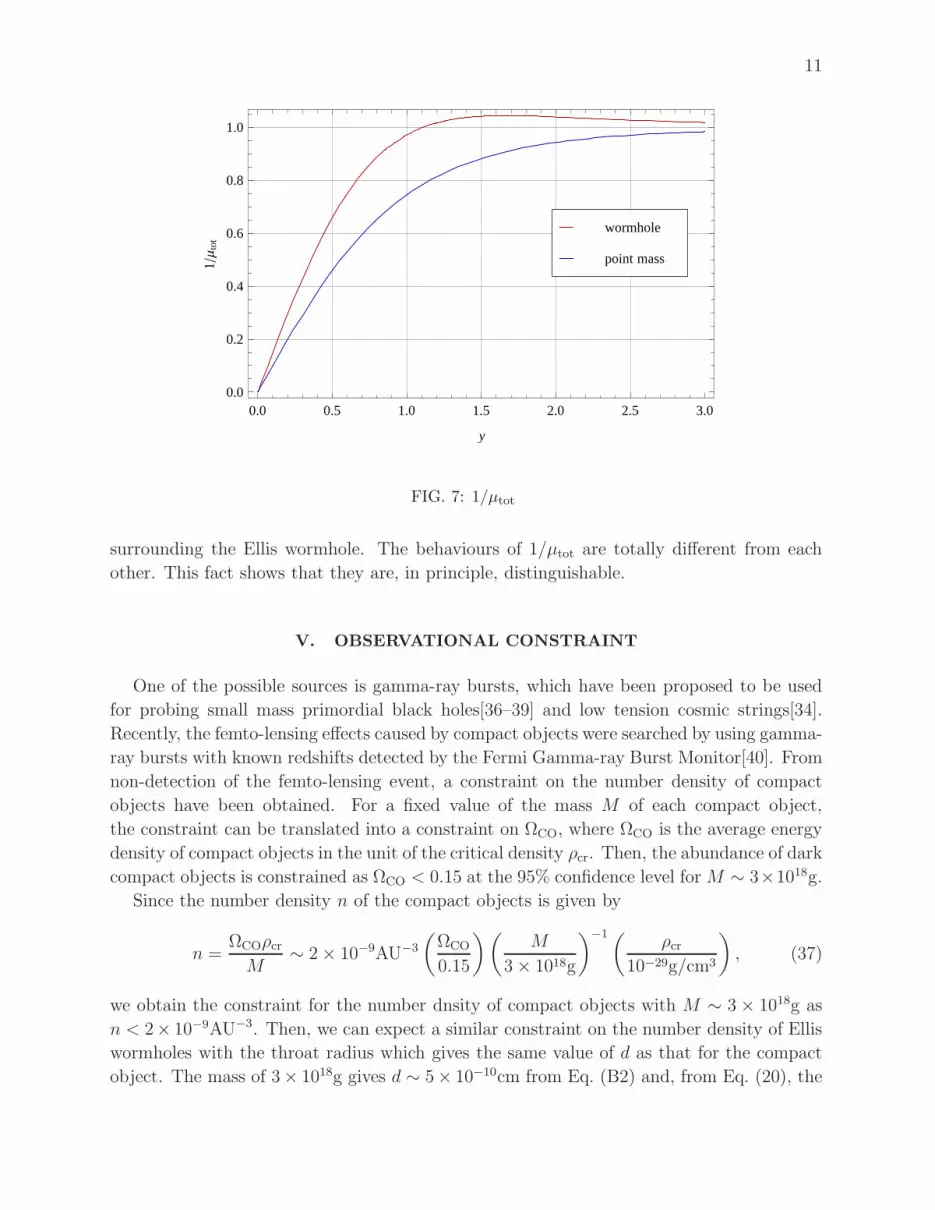
11
0.0 0.5 1.0 1.5 2.0 2.5 3.00.0
0.2
0.4
0.6
0.8
1.0
y
1Μ
tot
point mass
wormhole
FIG. 7: 1/µtot
surrounding the Ellis wormhole. The behaviours of 1/µtot are totally different from each
other. This fact shows that they are, in principle, distinguishable.
V. OBSERVATIONAL CONSTRAINT
One of the possible sources is gamma-ray bursts, which have been proposed to be used
for probing small mass primordial black holes[36–39] and low tension cosmic strings[34].
Recently, the femto-lensing effects caused by compact objects were searched by using gamma-
ray bursts with known redshifts detected by the Fermi Gamma-ray Burst Monitor[40]. From
non-detection of the femto-lensing event, a constraint on the number density of compact
objects have been obtained. For a fixed value of the mass M of each compact object,
the constraint can be translated into a constraint on ΩCO, where ΩCO is the average energy
density of compact objects in the unit of the critical density ρcr. Then, the abundance of dark
compact objects is constrained as ΩCO < 0.15 at the 95% confidence level for M ∼ 3×10¹⁸g.
Since the number density n of the compact objects is given by
n =ΩCOρcrM
∼ 2× 10⁻⁹AU−3
(
ΩCO
0.15
)(
M
3× 10¹⁸g
)−1(ρcr
10−29g/cm3
)
, (37)
we obtain the constraint for the number dnsity of compact objects with M ∼ 3 × 10¹⁸g as
n < 2× 10⁻⁹AU−3. Then, we can expect a similar constraint on the number density of Ellis
wormholes with the throat radius which gives the same value of d as that for the compact
object. The mass of 3× 10¹⁸g gives d ∼ 5× 10⁻¹⁰cm from Eq. (B2) and, from Eq. (20), the

12
corresponding throat radius a is given by
a ∼ 0.7cm
(
d
5× 10⁻¹⁰cm
)3/4(D
1028cm
)1/4
. (38)
Therefore, the number density of Ellis wormholes with a ∼ 1cm must satisfy n . 10−9AU−3.
Note that this constraint comes from the wave form in the geometrical optics approximation
and hence we do not distinguish between the point mass lenses and Ellis wormholes.
Another possible observation to probe Ellis wormholes is the observation of gravitational
waves from compact object binaries. The unlensed wave form of the gravitational waves from
a compact object binary is well known. From the chirp signal in the inspiral phase, we can
obtain the spectrum of the gravitational waves. In order to distinguish the Ellis wormhole
from a point mass lens, we need to observe not only the typical interference pattern but also
the wave effect in the lensed spectrum. Hence, the spectrum in d ∼ λ := 2π/ω is necessary
to probe the Ellis wormhole. Assuming d ∼ λ, the typical throat radius of Ellis wormholes
which can be probed by using gravitational waves is estimated as follows:
a = d3/4(
2D
π2
)1/4
∼ λ3/4
(
2D
π2
)1/4
∼ 7× 1012cm
(
λ
108cm
)3/4(D
1028cm
)1/4
. (39)
The same estimate is applicable for galactic sources of electro-magnetic waves. We obtain
a ∼ 105cm for galactic radio sources with λ ∼ 1cm, a ∼ 1m for galactic optical or infra-red
sources and a ∼ 1cm for galactic X-ray sources. The source must be compact enough to
show the clear oscillation behaviour in the spectrum. This fact can be clearly understood
by considering the y dependence of the phase in the amplification factor (33). Since τ(y)
is roughly approximated by 2y, the period δy for one cycle is given by δy ∼ π/(ωd). The
corresponding length scale δη on the source plane is given by
δη = δyDS
DLξ0 ∼
π
ω
√
2DLSDS
dDL
∼
√
λDLSDS
2DL
∼ 2× 1011cm
(
λ
1cm
)1/2(DLSDS/DL
10kpc
)1/2
, (40)
where we have assumed d ∼ λ. If the source radius is larger than δη, the interference
pattern will be smeared out. Observation of compact galactic sources such as pulsars and
white dwarfs might be useful to probe not only dark compact objects but also exotic compact
objects such as the Ellis wormhole.
VI. SUMMARY
In this paper, we have proposed the probe of Ellis wormholes by using spectroscopic
observations. We have assumed that the spectrum of the target source can be measured in

13
enough accuracy and the spectrum shape is well known without lensing, but the luminosity
is not necessarily observable. Then, we have discussed the distinguishability of the lensed
spectrum from the case of the point mass lens.
We have derived the wave form after the scattering by the Ellis wormhole including the
wave effect in the low frequency domain. The geometrical optics limit of the wave form
has been also analytically derived. Then, we have found that the Ellis wormhole cannot be
distinguished from the point mass lens by using only the high frequency domain in which
the geometrical optics approximation is valid. We have also found that this degeneracy is
resolved in the low frequency domain in which the wave effect is significant. Possible obser-
vational constraints are also discussed and we estimated the upper bound for the number
density of Ellis wormholes as n . 10−9AU−3 with throat radius a ∼ 1cm from the existing
femto-lensing analysis for compact objects.
Finally, we note that our method to probe the Ellis wormhole is complementary to the
other methods to probe the Ellis wormhole with micro-lensing [21–23] or the astrometric
image centroid displacements[26]. These are not feasible for observations on cosmological
scales because the time scale of the lens event is too long to detect modulation of the
light curve or the displacements. In contrast, the slow relative motion is an advantage for
spectroscopic observations. Therefore we may probe the Ellis wormhole on cosmological
scales using our method.
Acknowledgements
CY is supported by a Grant-in-Aid through the Japan Society for the Promotion of
Science (JSPS). The work of NT was supported in part by Rikkyo University Special Fund for
Research. TH was supported by the Grant-in-Aid for Young Scientists (B) (No. 21740190)
and the Grant-in-Aid for Challenging Exploratory Research (No. 23654082) for Scientific
Research Fund of the Ministry of Education, Culture, Sports, Science and Technology, Japan.
Appendix A: Derivation of Eq. (14)
The first term in Eq. (13) can be evaluated as follows.
∫ B
S
dl = |−→SA|+ |
−→AB| = |
−→SA|+ |
−→OA−
−→OB|
= |−→SA|+
√
|−→OA|2 + |
−→OB|2 − 2
−→OA ·
−→OB. (A1)
−→OB and
−−→OB′ can be written as
−→OB =
[
(
1−δD
DL
)
−→OL + ~η +
(
~ξ − ~η) DLS + δD
DLS
− αδD~ξ
ξ
]
(1 +O(ǫ3))

14
=
[
(
1−δD
DL
)
−→OL + ~ξ − α(ξ)δD
~ξ
ξ+(
~ξ − ~η) δD
DLS
]
(1 +O(ǫ3)), (A2)
−−→OB′ =
(
1−δD
DL
)
−→OA. (A3)
From these expressions, we can find
|−→OB| = |
−−→OB′|
(
1 +O(ǫ3))
, (A4)−→OA ·
−→OB =
−→OA ·
−−→OB′
(
1 +O(ǫ3))
. (A5)
Therefore we obtain
∫ B
S
dl =(
|−→SA|+ |
−→OA| − |
−−→OB′|
)
(
1 +O(ǫ3))
. (A6)
Since we find
|−→SA| =
√
|~ξ − ~η|2 +D2LS = DLS
(
1 +|~ξ − ~η|2
2D2LS
+O(ǫ4)
)
, (A7)
|−→AO| = DL
(
1 +ξ2
2D2L
+O(ǫ4)
)
, (A8)
we obtain the following expression:
∫ B
S
dl =
DS
(
1 +η2
2D2S
)
+DLDS
2DLS
(
~ξ
DL
−~η
DS
)2
− r
(
1 +O(ǫ3))
, (A9)
where r = |−−→OB′|.
In order to evaluate the second term in Eq. (13), we first consider the integral between S
and A. Letting P be a point on the segment SA, we obtain
|−→LP|2 = |~ξ +
−→AP|2 =
∣
∣
∣
∣
~ξ +
(
1−l
lSA
)
−→AS
∣
∣
∣
∣
2
= ξ2 + (lSA − l)2 + 2
(
1−l
lSA
)
~ξ ·−→AS, (A10)
where lSA = |−→SA| and l = |
−→SP|. Since ~ξ ·
−→AS = −~ξ ·(~ξ−~η), we obtain the following expression:
|−→LP|2 = ξ2 + (lSA − l)2 − 2
(
1−l
lSA
)
~ξ · (~ξ − ~η). (A11)
Substituting the above expression of |−→LP|2 into R2 of the second integral in Eq. (13) with
the integral region being from S to A, we obtain
∫ A
S
1
R2dl =
∫ lSA
0
dl
ξ2 + (lSA − l)2 − 2(1− llSA
)~ξ · (~ξ − ~η). (A12)
15
Then the integral (A12) can be performed and evaluated as
∫ lSA
0
dl
(lSA − l)2 + ξ2 − 2(1− llSA
)~ξ · (~ξ − ~η)=
lSAξDLS
[
arctan
(
−l2SA + ~ξ · (~ξ − ~η) + llSAξDLS
)]lSA
0
=
(
π
2ξ−
~ξ · ~η
ξ2DLS
)
(
1 +O(ǫ2))
. (A13)
The contribution from the integral between A and B can be also evaluated by the similar
integral. Finally, we obtain the expression (14).
Appendix B: Point Mass Lens
For the point mass case, we have the following expression for the amplification factor [28,
29]:
|F po| =∣
∣eπωd/2Γ (1− iωd) 1F1 (iωd, 1; iωdy)∣
∣ , (B1)
where Γ and 1F1 are the gamma function and the confluent hyper-geometric function, re-
spectively, and
d = 2M, y = η
√
DL
4MDLSDS
. (B2)
In the geometrical optics approximation (ω → ∞), we obtain
|F po|2 →∣
∣F pogeo
∣
∣
2:= |µpo
+ |+ |µpo− |+ 2
√
|µpo+ µpo
− | sin(2ωdτpo(y)), (B3)
where
µpo± = ±
1
4
[
y√
y2 + 4+
√
y2 + 4
y± 2
]
, (B4)
τpo(y) =1
2y√
y2 + 4 + ln
√
y2 + 4 + y√
y2 + 4− y. (B5)
|F po|2 and |F pogeo|
2 are depicted as functions of ω for each value of y in Fig. 8.
[1] MACHO Collaboration, C. Alcock et al., Astrophys.J. 542, 281 (2000),
arXiv:astro-ph/0001272, The MACHO project: Microlensing results from 5.7 years of
LMC observations.
[2] EROS-2 Collaboration, P. Tisserand et al., Astron.Astrophys. 469, 387 (2007),
arXiv:astro-ph/0607207, Limits on the Macho Content of the Galactic Halo from the EROS-2
Survey of the Magellanic Clouds.

16
0.05 0.10 0.50 1.00 5.00 10.000.7
0.8
0.9
1.0
1.1
1.2
1.3
1.4
Ω @1TD
ÈFpo
2
y=2
ÈFgeopo 2
ÈFpo 2
0.05 0.10 0.50 1.00 5.00 10.00
0.5
1.0
1.5
2.0
Ω @1TD
ÈFpo
2
y=1
ÈFgeopo 2
ÈFpo 2
0.05 0.10 0.50 1.00 5.00 10.000
1
2
3
4
Ω @1TD
ÈFpo
2
y=12
ÈFgeopo 2
ÈFpo 2
0.05 0.10 0.50 1.00 5.000
5
10
15
20
Ω @1TD
ÈFpo
2
y=110
ÈFgeopo 2
ÈFpo 2
FIG. 8: |F po|2 and |F pogeo|2 as functions of ω for each value of y, where T = d τpo.
[3] L. Wyrzykowski et al., Mon.Not.Roy.Astron.Soc. 397, 1228 (2009), arXiv:0905.2044, The
OGLE View of Microlensing towards the Magellanic Clouds. I. A Trickle of Events in the
OGLE-II LMC data.
[4] D. Huterer and T. Vachaspati, Phys.Rev. D68, 041301 (2003), arXiv:astro-ph/0305006, Grav-
itational lensing by cosmic strings in the era of wide - field surveys.
[5] M. Oguri and K. Takahashi, Phys.Rev. D72, 085013 (2005), arXiv:astro-ph/0509187, Char-
acterizing a cosmic string with the statistics of string lensing.
[6] K. J. Mack, D. H. Wesley, and L. J. King, Phys.Rev. D76, 123515 (2007),
arXiv:astro-ph/0702648, Observing cosmic string loops with gravitational lensing surveys.
[7] K. Kuijken, X. Siemens, and T. Vachaspati, MNRAS384, 161 (2008), arXiv:0707.2971, Mi-
crolensing by cosmic strings.
[8] J. Christiansen et al., Phys.Rev. D83, 122004 (2011), arXiv:1008.0426, Search for Cosmic
Strings in the COSMOS Survey.
[9] A. Tuntsov and M. Pshirkov, Phys.Rev. D81, 063523 (2010), arXiv:1001.4580, Quasar vari-
ability limits on cosmological density of cosmic strings.
[10] M. Pshirkov and A. Tuntsov, Phys.Rev. D81, 083519 (2010), arXiv:0911.4955, Local con-

17
straints on cosmic string loops from photometry and pulsar timing.
[11] D. Yamauchi, K. Takahashi, Y. Sendouda, and C.-M. Yoo, Phys.Rev. D85, 103515 (2012),
arXiv:1110.0556, Weak lensing of CMB by cosmic (super-)strings.
[12] D. Yamauchi, T. Namikawa, and A. Taruya, JCAP 1210, 030 (2012), arXiv:1205.2139, Weak
lensing generated by vector perturbations and detectability of cosmic strings.
[13] H. Ellis, J.Math.Phys. 14, 104 (1973), Ether flow through a drainhole - a particle model in
general relativity.
[14] H.-a. Shinkai and S. A. Hayward, Phys.Rev. D66, 044005 (2002), arXiv:gr-qc/0205041, Fate
of the first traversible wormhole: Black hole collapse or inflationary expansion.
[15] A. Das and S. Kar, Class.Quant.Grav. 22, 3045 (2005), arXiv:gr-qc/0505124, The Ellis worm-
hole with ‘tachyon matter’.
[16] L. Chetouani and G. Clement, General Relativity and Gravitation 16, 111 (1984), Geometrical
optics in the Ellis geometry.
[17] G. Clement, International Journal of Theoretical Physics 23, 335 (1984), Scattering of Klein-
Gordon and Maxwell Waves by an Ellis Geometry.
[18] K. Nakajima and H. Asada, Phys.Rev. D85, 107501 (2012), arXiv:1204.3710, Deflection angle
of light in an Ellis wormhole geometry.
[19] N. Tsukamoto and T. Harada, (2012), arXiv:1211.0380, Signed magnification sums for general
spherical lenses.
[20] D. F. Torres, G. E. Romero, and L. A. Anchordoqui, Phys.Rev. D58, 123001 (1998),
arXiv:astro-ph/9802106, Might some gamma-ray bursts be an observable signature of natu-
ral wormholes?
[21] M. Safonova, D. F. Torres, and G. E. Romero, Phys.Rev. D65, 023001 (2002),
arXiv:gr-qc/0105070, Microlensing by natural wormholes: Theory and simulations.
[22] M. Bogdanov and A. Cherepashchuk, Astrophys.Space Sci. 317, 181 (2008), arXiv:0807.2774,
Search for exotic matter from gravitational microlensing observations of stars.
[23] F. Abe, Astrophys.J. 725, 787 (2010), arXiv:1009.6084, Gravitational Microlensing by the
Ellis Wormhole.
[24] H. Asada, Prog.Theor.Phys. 125, 403 (2011), arXiv:1101.0864, Gravitational microlensing in
modified gravity theories: Inverse-square theorem.
[25] T. Kitamura, K. Nakajima, and H. Asada, (2012), arXiv:1211.0379, Demagnifying gravita-

18
tional lenses toward hunting a clue of exotic matter and energy.
[26] Y. Toki, T. Kitamura, H. Asada, and F. Abe, Astrophys.J. 740, 121 (2011), arXiv:1107.5374,
Astrometric Image Centroid Displacements due to Gravitational Microlensing by the Ellis
Wormhole.
[27] N. Tsukamoto, T. Harada, and K. Yajima, (2012), arXiv:1207.0047, Can we distinguish
between black holes and wormholes by their Einstein ring systems?
[28] S. Deguchi and W. D. Watson, Phys.Rev. D34, 1708 (1986), Wave effects in gravitational
lensing of electromagnetic radiation.
[29] P. Schneider, J. Ehlers, and E. E. Falco, Gravitational Lenses (, 1992).
[30] C. Baraldo, A. Hosoya, and T. T. Nakamura, Phys. Rev. D59, 083001 (1999), Gravitationally
induced interference of gravitational waves by a rotating massive object.
[31] A. Mehrabi and S. Rahvar, arXiv:1207.4034 [astro-ph.EP].
[32] R. Takahashi and T. Nakamura, Astrophys. J. 595, 1039 (2003), astro-ph/0305055, Wave
effects in gravitational lensing of gravitational waves from chirping binaries.
[33] T. Suyama, T. Tanaka, and R. Takahashi, Phys.Rev. D73, 024026 (2006),
arXiv:astro-ph/0512089, Exact wave propagation in a spacetime with a cosmic string.
[34] C.-M. Yoo, R. Saito, Y. Sendouda, K. Takahashi, and D. Yamauchi, (2012), arXiv:1209.0903,
Femto-lensing due to a Cosmic String.
[35] M. Born and E. Wolf, Principles of Optics (, 1999).
[36] A. Gould, ApJ386, L5 (1992), Femtolensing of gamma-ray bursters.
[37] K. Z. Stanek, B. Paczynski, and J. Goodman, ApJ413, L7 (1993), Features in the spectra of
gamma-ray bursts.
[38] A. Ulmer and J. Goodman, Astrophys.J. 442, 67 (1995), arXiv:astro-ph/9406042, Femtolens-
ing: Beyond the semiclassical approximation.
[39] G. Marani, R. Nemiroff, J. Norris, K. Hurley, and J. Bonnell, (1998), arXiv:astro-ph/9810391,
Gravitationally lensed gamma-ray bursts as probes of dark compact objects.
[40] A. Barnacka, J. Glicenstein, and R. Moderski, Phys.Rev. D86, 043001 (2012),
arXiv:1204.2056, New constraints on primordial black holes abundance from femtolensing of
gamma-ray bursts.