water budgets of two watersheds in different climatic zones under projected climate warming

WATER BUDGETS OF TWO WATERSHEDS IN DIFFERENT CLIMATICZONES UNDER PROJECTED CLIMATE WARMING

OMID MOHSENI and HEINZ G. STEFANUniversity of Minnesota, St. Anthony Falls Laboratory, Mississippi River at 3rd Ave. SE,

Minneapolis, MN 55414, U.S.A.E-mails: [email protected] and [email protected]

Abstract. A deterministic monthly runoff model (MINRUN96) was applied to watersheds withsubstantially different climates. One watershed is in the north-central U.S. (Minnesota) and is heavilytimbered. The other is in the south-central U.S. (Oklahoma) and is mainly covered with pasturesand agricultural crops. Runoff was simulated for past historical climate and two projected 2× CO2climate scenarios. The output of General Circulation Models (GCMs) was used to specify the two2 × CO2 climate scenarios. One GCM is the Goddard Institute of Space Studies (GISS) modeland the other is from the Canadian Center of Climate Modelling (CCC). In the northern watershedmore runoff is projected to occur in winter under a warmer climate and less runoff in spring. About80% increase in fall runoff and 20% decrease in soil moisture in June and July is projected for thesouthern watershed. When runoff simulations for the 2× CO2 climate scenarios were compared topast runoff, it was apparent that the change in runoff depended on both the season and the magnitudeof the precipitation change. An increase in spring precipitation caused a significant increase in directrunoff, whereas an increase in fall precipitation caused only a slight increase in total runoff. Also therunoff-precipitation relationship in the warm and seasonally dry southern watershed is very differentfrom that in the temperate and humid climate of the north. Therefore, runoff responses to projectedclimate change are substantially different in the two regions.

1. Introduction

The measured and projected increase of carbon dioxide in the atmosphere has be-come an important environmental issue. It is anticipated that atmospheric CO2 willdouble in the next century (NRC, 1982, 1983), and the impact on natural resourcesneeds to be studied. Herein we focus on fresh water resources, especially the effectof climate change on streamflow.

Streamflow depends on climate variables such as precipitation, air temperature,solar radiation, humidity and wind speed, and watershed parameters such as landuse and surface soil moisture content. Therefore, if there is a reliable projection ofthe future climate of a region, it may be possible to project the resulting change insurface runoff.

The scope of this paper is to project the mean monthly streamflow of two riversin the U.S. under three different climate scenarios, one being the observed climateand the other two forecast by two general circulation models (GCMs) for a 2×CO2 atmosphere (an atmosphere with a doubled concentration of carbon dioxide).

Climatic Change49: 77–104, 2001.© 2001Kluwer Academic Publishers. Printed in the Netherlands.

78 OMID MOHSENI AND HEINZ G. STEFAN

The two streams are located in different climatic zones of the central U.S., one inMinnesota and the other in Oklahoma. The characteristics of each will be describedlater. The streamflow model used in this study is a deterministic, monthly time scalemodel.

2. Previous Studies

A variety of models have been used to project streamflow from watersheds un-der different climate scenarios. Some models projected the changes in streamflowbased on perturbations in temperature, precipitation or evapotranspiration whileothers used the climate projections of GCMs as input. One may categorize themodels used as either monthly or daily time scale runoff models. Gleick (1987a)modified the Thornthwaite–Mather (1955) monthly runoff model by adding a cal-ibrated storm component. He applied the model to the Sacramento River basinand projected on average 35% increase in winter runoff and 45% decrease insummer runoff, using different climate projections of GCMs as input (Gleick,1987b). McCabe and Ayers (1989) used the original Thornthwaite–Mather (1955)model and applied it to the Delaware River watershed, the region for which themodel was originally developed. They projected different runoff trends using threedifferent GCMs. Overall, they projected a decrease in annual runoff. Newman etal. (1992) studied the effects of the GISS GCM climate projections on 9 water-sheds in Minnesota by applying the original Thornthwaite–Mather (1955) waterbudget model. Newman et al. (1992) projected a significant decrease in springand summer runoff and an increase in winter runoff. Schaake (1990) developeda simple nonlinear monthly water balance model and applied it to 52 basins in thesoutheastern U.S. for regional climate change studies. He projected the regionalrunoff for changes in evapotranspiration and precipitation. Rao et al. (1995) used amonthly time scale runoff model (Mimikou et al., 1990) and projected the climatechange effects in the Wabash River basin in Indiana. They did not use the outputof GCMs but formulated their own selective scenarios for temperature and pre-cipitation change. Xu and Halldin (1997) applied a simple monthly water balancemodel to 11 catchments in the NOPEX area under a number of climate changescenarios. They showed that a 20% increase in annual precipitation would result in31–51% increase in annual runoff. Lettenmaier et al. (1990) combined a snowmeltmodel (Anderson, 1973) with a soil moisture accounting model (Burnash et al.,1973), applied it to four subbasins of the Sacramento–San Joaquin River basin,and forecast climate change effects on the streamflow of the watersheds, using theoutput of three GCMs. They projected a significant increase in winter runoff anda small decrease in summer runoff. Singh and Kumar (1997) applied the UBCwatershed model to project changes in glacier melt runoff, snowmelt runoff andtotal runoff in a Himalayan river under different perturbations in temperature and

WATER BUDGETS OF TWO WATERSHEDS UNDER CLIMATE WARMING 79

precipitation. They projected that total streamflow would increase linearly withboth temperature and precipitation.

These studies generally involved the application of a specific model to water-sheds in a particular climate region. Only the Thornthwaite–Mather (1955) runoffmodel was applied to watersheds in different climatic zones. The Thornthwaite–Mather (1955) model was not validated for the rivers in Minnesota and had adifferent structure when applied to the Delaware and Sacramento River basins.Herein, a single model is applied to watersheds in two different climatic zones toassess the similarities and differences in response to 2× CO2 climate conditions.

The time scale and the spatial scale of the hydrologic model are importantconsiderations. Because the GCMs provide monthly values of weather parameterchanges at global grid points, which are on average 5◦ apart, one has difficulty touse these values on a watershed scale and a daily time scale. The temporal andspatial variability of precipitation, more than any other weather parameter, makesit however difficult to forecast runoff using the values at such GCM grid pointsand at a monthly time scale. There have been efforts to estimate the temporal andspatial variability of climate parameters within the GCM grid cells by using eitherregional climate models (Giorgi et al., 1994, 1998; Hostetler and Giorgi, 1995)or statistical downscaling methods (Wilks, 1992; von Storch et al., 1993; Hughesand Guttorp, 1994; Zorita et al., 1995). Both physics-based and stochastic modelsenhance, however, the uncertainties embedded in the forecast of 2× CO2 climateconditions.

A monthly time scale runoff model is compatible with the monthly output ofthe GCMs and spatial variability of precipitation within a grid cell is reduced atthe monthly time scale. Monthly runoff models also require less input data thandaily models and fewer calibration coefficients. Monthly or seasonal time scalesare widely used for watershed management and planning. Therefore, a monthlydeterministic model (MINRUN96) is used herein to study the effect of the 2×CO2

climate conditions on runoff. This model has been used to successfully simulatemonthly runoffand other water budget components of watersheds (Mohseni andStefan, 1998).

3. Streamflow Model

To devise a single model which requires minimum input data and can simulatestreamflow in both the cold regions of the northern U.S. and the semi-arid re-gions of the southwestern U.S. is a difficult task (Schaake, 1990). Snowmelt inthe northern regions requires very different model formulations and/or use of verydifferent calibration coefficients than intermittent storm runoff in southern regions.The interdependence of model parameters creates difficulties in the calibrationof such a model (Sorooshian and Gupta, 1983). The available runoff models areoften either simplistic and can only be applied to the regions for which they were


originally developed, or they are complex and have parameterized the hydrolo-gic processes using numerous interdependent calibration coefficients. Calibratingthese latter models is a difficult and sometimes an unmanageable task.

The runoff model used (Mohseni and Stefan, 1998) contains deterministic re-lationships to estimate four components of streamflow: Direct runoff, interflow,base flow and snowmelt. The model input is divided into two categories: Water-shed characteristics and meteorological data. Watershed characteristics include: (a)the physiography of the watershed (i.e., its area, total length of streams, averageoverland slope and percentage of forest cover), (b) soil characteristics such as thesaturation hydraulic conductivity, field capacity, wilting point and porosity, and(c) type of vegetation cover and the stage of growth. Meteorological data includeprecipitation, air temperature, dew point temperature, solar radiation, cloud coverand wind velocity. The model also requires the average number of rainy days ineach month as input, which can be calculated from the historical rainfall data. Themodel has four calibration coefficients: (1) the thickness of the uppermost layer ofthe surface soil which controls direct runoff, (2) the average number of rainy dayswhich produce storm runoff in each month, (3) the critical net radiation for thebeginning of snowmelt, and (4) a shading factor for snowmelt.

Following is a brief description of different components of the streamflowmodel (Mohseni and Stefan, 1998).

3.1. DIRECT RUNOFF

If there is rainfall, the model determines if there is any direct runoff. The conditionfor direct runoff comes from the comparison of the moisture deficit (with respectto the saturation content) of the uppermost layer of the surface soil,Fj = D1θj ,with the average daily rainfall,Pj/Nj . The parametersD and1θj are the thicknessand the average daily moisture deficit of the surface soil (cm3/cm3), respectively.Direct monthly runoff,Qd , is the average excess daily rainfall in a month times theaverage number of rainy days which become runoff,Mj , i.e.,

Qd,j = Mj

(Pj

Nj− Fj

). (1)

Direct runoff is simulated best whenM is calibrated, since calibratingM capturesother shortcomings of the infiltration/direct runoff parameterization. The thicknessof the uppermost layer of the surface soil is also obtained through calibration.

3.2. INTERFLOW

The rainfall which infiltrates into the root zone contributes to evapotranspiration.Evapotranspiration is estimated using the Penman–Monteith equation, which usescrop cover and soil moisture content as parameters. If the infiltration rate is largerthan the evapotranspiration rate, and if the moisture content in the root zone ex-ceeds the field capacity, some of the infiltrated water appears again on the surface


as interflow and contributes to the monthly streamflow; the rest joins the stor-age below the root zone. The fraction of the excess moisture content in the rootzone, which becomes interflow within a time step is estimated using the followingequation

β = 1.44LKsSoφA

, (2)

whereA is the area of the watershed (km2), L is total length of streams (km),So isthe average overland slope of the watershed,φ is porosity andKs is the saturationhydraulic conductivity of the root zone (m/hr).

3.3. BASE FLOW

The storage below the root zone (SBR) contains a saturated zone (the shallowaquifer) and an unsaturated zone (the layer between the root zone and the shallowaquifer). Whatever percolates into SBR adds to the overall moisture content of thezone but does not contribute to streamflow until the next time step (next month).When SBR exceeds field capacity then there will be base flow; base flow is estim-ated using the parameterβ introduced in Equation (2). Since in Equation (2), thepiezometric head gradient of the SBR is set equal to the average overland slope ofthe watershed, the hydraulic conductivity is set equal to the average unsaturatedhydraulic conductivity of the entire SBR. If SBR exceeds saturation, the extramoisture percolates into the deep aquifer. In this paper, the sum of base flow andinterflow is presented as subsurface flow.

3.4. SNOWFALL AND SNOWMELT

The runoff model divides the monthly precipitation into rainfall and snowfall ac-cording to air temperature. If monthly air temperature is below –1◦C the entiremonthly precipitation is set to be snowfall. This threshold temperature was ob-tained through trial and error. A –1◦C threshold temperature has also been usedby U.S. Army Corps of Engineers (1956) and van Hylckama (1956). The modelkeeps track of snow accumulation on the ground. Snowmelt occurs if monthly netradiation is larger than a critical value. There can be snowmelt in months withtemperatures below freezing if the net radiation is high enough. The critical netradiation is obtained by calibration. The snowmelt rate is a function of net radiationand the shading factor of the watershed. Shading can be either due to the vegetationcover, e.g., in forested regions, or due to the watershed topography, which restrainsthe duration of solar radiation. In this model, the shading factor is obtained bycalibration.


Figure 1.Geographical locations of the Baptism River and the Little Washita River watersheds in theU.S.

4. Watersheds and Model Calibration

The runoff model was applied to two watersheds, the Baptism River and the LittleWashita River. The Baptism River watershed (Figure 1) with an area of 363 squarekilometers (140 mi2) is located in northern Minnesota (at 47.5◦ latitude and 91.3◦longitude). It discharges 420 mm of water annually into Lake Superior. The meanannual precipitation in the watershed is 770 mm. The watershed is heavily timberedwith both deciduous and coniferous trees. The average overland slope is less than4% and the surface soil is shallow and mainly glacial drift. Snow accumulationstarts in November and snowmelt starts in March and continues to mid May.

There is no weather station within the watershed. The weather data, with the ex-ception of air temperature and precipitation, were obtained from the Duluth Airportabout 80 km away. Air temperature and rainfall data were from the gage at Isabella.Data collection at Isabella started in September 1957. The period 1961–1979 waschosen to represent the 1× CO2 (past) climate conditions. This period containsboth dry and wet years. In order to fill in a few missing monthly precipitation dataa multiple linear regression analysis between the Isabella station and four other


Figure 2.(a) Simulated and observed mean monthly streamflow and mean monthly recorded precip-itation in the Baptism River watershed for the period 1961–1979. (b) Mean monthly runoff changesin the Baptism River watershed under 2× CO2 climate scenarios.

stations around Isabella (Brimson, Babbitt 2 SE, Winton Power Plant and GrandMarais) was done for the period 1958–1990. The watershed characteristics arelisted in Table I. The runoff model was initially calibrated for the period 1966–1979with data for the Baptism River watershed (Mohseni and Stefan, 1998). Figure 2ashows a comparison between the simulated and the observed mean monthly runofffor the period 1961–1979. The ratio of annual simulated runoff to observed runoffis 0.96. The calibration coefficients were kept unaltered for the application to the2× CO2 climate scenarios.


TABLE I

Watershed characteristics

Watershed Baptism Little Washita

Type Forested Agricultural

Area (km2) 363 538

Total length of streams (km) 200 350

Average overland slope (%) 3.6 4.8

Percentage of forest cover (%) 95 5

Saturation hydraulic conductivity (m/hr) 0.60 0.09

Soil moisture content at field capacity 0.150 0.260

Soil moisture content at wilting point 0.060 0.060

Soil porosity 0.350 0.360

The Little Washita River watershed (Figure 1) with an area of 538 square kilo-meters (208 mi2) is located in Oklahoma (34.9◦ latitude and 98◦ longitude). It isa tributary of the Washita River, which is in the Red River drainage basin. Meanannual streamflow at gage 522, for the period 1966–1983, is 49 mm. The meanannual precipitation in the watershed, for the same period, is 748 mm. The LittleWashita is an agricultural watershed. One third of the watershed is cultivated andthe rest is either pasture or wooded pasture. The average overland slope is 5% andthe surface soil is typically sandy loam and silty loam.

The Little Washita River watershed has been used as an experimental watershed.Climate variables are recorded at a number of stations throughout the watershedand soil variables (Table I) have been mapped for the entire watershed (Allen andNaney, 1991). Representative precipitation data of the entire watershed were ob-tained from five rain gages within the watershed using the Thiessen method (Shaw,1983). Mean monthly air temperatures and wind velocities were extracted from thedata collected at gage 124, in the northern section of the watershed. Solar radiationand dew point temperature were obtained from the Oklahoma City weather station.Streamflow was measured at stream gage 522 during the period 1966–1983. Themodel was initially calibrated for the period 1966–1979 with data for the LittleWashita River watershed (Mohseni and Stefan, 1998). Figure 3a shows a compar-ison between the simulated and the observed mean monthly runoff for the period1966–1979. The ratio of annual simulated runoff to observed runoff is 1.0.


Figure 3. (a) Simulated and observed mean monthly streamflow and mean monthly recorded pre-cipitation in the Little Washita River watershed for the period 1966–1979. (b) Mean monthly runoffchanges in the Little Washita River watershed under 2× CO2 climate scenarios.

To measure the goodness of fit between model simulations and observations theNash–Sutcliffe coefficient (NSC) (Nash and Sutcliffe, 1970), which is defined as

NSC= 1−

n∑i=1

(Qsimi −Qobsi )2

n∑i=1

(Q̄obs−Qobsi )2

(3)


with a maximum of 1.0 as a perfect fit and a minimum of –∞, was calculatedfor the calibration period 1961–1979 for the Baptism River and 1966–1979 forthe Little Washita River. In Equation (3),Qsim is simulated monthly runoff,Qobs isobserved monthly runoff and̄Qobs is the average of observed monthly streamflows.For monthly runoff in the Baptism River and the Little Washita River, NSC was0.68 and 0.79, respectively, and for mean monthly runoff, NSC was 0.99 and 0.94,respectively.

5. 2× CO2 Climate Scenarios

The outputs from the GCMs developed at the Goddard Institute of Space Studies(GISS) (Hansen et al., 1983) and the Canadian Climate Center (CCC) (McFarlaneet al., 1992) were used to specify the 2×CO2 (equilibrium) climate scenarios. TheGISS-GCM is a finite difference atmospheric model with a grid size of 7.83◦×10◦.?The CCC GCMII is a spectral coupled atmosphere-ocean model with a grid size of3.75◦ × 3.75◦. The monthly changes in two weather parameters (air temperatureand precipitation) predicted by both GCMs for a 2× CO2 climate scenario andused for both watersheds are displayed in Figures 4 and 5. The changes are shownas increments in◦C for air temperature and percentage change for precipitation.

For the Baptism River, differences between the output of the two GCMs areevident throughout the year. There is a 2–3◦C difference in the projected Janu-ary and February air temperature changes (Figures 4a,b). The CCC-GCM projectsslightly more precipitation in winter and early spring while the GISS model showsa significant increase in precipitation in summer and fall (Figures 4c,d). Annualprecipitation, according to the GISS output, increases by 24%, but the CCC outputgives only 1% increase (Table II). Other variables are not projected to changesignificantly except the wind velocity.

In the Little Washita River, air temperature changes in fall and early winterprojected by the GISS-GCM are 2–3◦C larger than those projected by the CCC-GCM (Figures 5a,b). Mean monthly air temperature increments projected by thetwo GCMs are more compatible in the Little Washita River watershed than inthe Baptism River watershed. For the Little Washita River watershed, the maindifference is in the precipitation values. The GISS-GCM shows a 130% increase inprecipitation in September and the CCC-GCM shows a 145% increase in October(Figures 5c,d). Consequently, there will probably be a one month difference intiming the fall peak runoff prediction.

? The GISS has developed a new model with finer resolution, 4◦×5◦. The new model is a coupledatmosphere-ocean model which has been used to study transient climate (Russell et al., 1995).


Figure 4.The mean monthly climate parameter changes under 2×CO2 scenarios in the Baptism Riverwatershed. (a) The CCC-GCM projection of mean monthly air temperature incremental changes, (b)the GISS-GCM projection of mean monthly air temperature incremental changes, (c) the CCC-GCMprojection of mean monthly precipitation changes in percentage, and (d) the GISS-GCM projectionof mean monthly precipitation changes in percentage.

6. Model Input

The input data to the runoff model are watershed characteristics including physio-graphic parameters, vegetation and soils information, and meteorological data. Nochange in the physiographic characteristics is expected under the 2× CO2 climatescenarios. Therefore, it was assumed that the soil properties and the thickness of


Figure 5.The mean monthly climate parameter changes under 2×CO2 scenarios in the Little WashitaRiver watershed. (a) The CCC-GCM projection of mean monthly air temperature incrementalchanges, (b) the GISS-GCM projection of mean monthly air temperature incremental changes, (c) theCCC-GCM projection of mean monthly precipitation changes in percentage, and (d) the GISS-GCMprojection of mean monthly precipitation changes in percentage.

the top soil, which was calibrated for 1961–1979, would remain unchanged. It wasalso assumed that no change would occur to the vegetation cover. This assumption,however, might be true for the agricultural watershed, but not necessarily for theforested watershed. The change in vegetation would affect potential evapotranspir-ation and the shading factor. The sensitivity analysis conducted for MINRUN96(Mohseni and Stefan, 1998) showed that a±20% change in shading factor had no


TABLE II

Mean annual changes in climate variables in the Baptism River watershed projected for a 2× CO2climate scenario by the CCC-GCM and the GISS-GCM

Parameters Observed 2× CO2 CCC-GCM 2× CO2 GISS-GCM

Absolute Absolute Change Absolute Change

value value value

Air temperature (◦C) 3.4 8.4 +5.0◦C 7.7 +4.3◦CDew point temperature (◦C) –2.0 2.9 +4.9◦C 2.5 +4.5◦CNet radiation (MJ/m2) 2500 2480 –1% 2560 +2%

Wind speed (m/sec) 3.5 3.3 –5% 3.4 –4%

Precipitation (mm) 769 779 +1% 958 +25%

effect on the annual runoff, but changed the distribution of snowmelt in late winterand spring by 10%. Since the GCMs used in this study had not archived changes infrequency of rainfall under 2×CO2 climate conditions, the average number of rainydays was kept unchanged for the 2×CO2 climate scenarios. The sensitivity analysisalso showed that the mean monthly runoff would change between 10–17% whentheM value of that month (the average number of rainy days in a month whichbecome runoff) was changed by±20%. However, the annual runoff changed byless than 1% in the Baptism River and between 0.4–3% in the Little Washita River.Finally, all the calibration coefficients were kept unchanged.

The meteorological input data consisted of air temperature, dew point temper-ature, solar radiation, percentage of cloud cover, wind velocity and precipitation.Using the output of the GCMs, air temperatures were incremented by the differencebetween the 2×CO2 and the 1×CO2 climate scenarios projected by GCMs. Solarradiation, specific humidity, wind velocity and precipitation were changed usingthe ratios of the 2× CO2 to 1× CO2 climate scenarios.

Results were obtained with adjusted meteorological data of the period 1961–1979 for the Baptism River and 1962–1979 for the Little Washita River to specifythe 2× CO2 climate scenario.

7. Model Results

To project the effects of a 2×CO2 climate scenario, the absolute changes in meanmonthly water budget components were calculated. To illustrate the statistical sig-nificance of these changes, two-tail paired-samplet-tests at a 10% significancelevel were conducted for all monthly values of the water budget components.Circles in the upper part of each figure illustrate that the difference between thesimulated past and the 2× CO2 climate scenario is statistically significant at the


10% significance level. The error bars show the standard deviation of the meanmonthly changes.

7.1. BAPTISM RIVER RUNOFF UNDER A2× CO2 CLIMATE SCENARIO

The projected mean monthly changes in runoff in the Baptism River watershedare illustrated in Figure 2b. Due to the advancing of the snowmelt season underglobal warming both the CCC and GISS 2× CO2 scenarios give an increase inrunoff in March, and a decrease in April and May. The changes projected under theCCC 2×CO2 climate scenario are, however, smaller and statistically insignificant.There is disagreement in the projected fall runoff because the GISS 2×CO2 climatescenario shows a doubling of precipitation in September (Figure 4d) but the CCCscenario does not. There would be about 20% increase (statistically significant) inwinter runoff under both 2× CO2 climate scenarios. The CCC 2× CO2 climatescenario projects a 7%decreasein mean annual runoff, but the GISS 2× CO2

scenario gives a 12%increase(Table IV). Mean annual changes in runoff are, how-ever, statistically insignificant. The differences in projected annual precipitation(Table II) can explain the annual differences in projected runoff.

Conversion of monthly rainfall to monthly runoff is basically non-linear dueto the effects of other processes such as infiltration and evapotranspiration. Forthose months in which snowmelt does not contribute to runoff, simulatedchangesin runoff againstchangesin rainfall are displayed in Figure 6. When monthlyrainfall increases or decreases by amounts less than 70 mm the runoff responseis non-linear and not well defined. As monthly rainfall changes exceed 70 mm, therelationship becomes linear and runoff increases are about 0.5 times the increasesin monthly rainfall. Therefore, the GISS scenario projects a significant increase infall runoff.

Figure 6 also shows that under the CCC 2× CO2 climate scenario, monthlystreamflow increases occur often concurrently with monthly precipitation de-creases. This is possible during the low flow season (fall and winter) when thestreamflow lags the precipitation that has recharged the aquifer in the precedingmonths. This is illustrated in Figures 7 and 8 which give the water budget compon-ents of the Baptism River watershed. Under the CCC 2× CO2 climate scenario,potential evapotranspiration is increased throughout the year (Figure 7b). Actualevapotranspiration, however, does not change significantly (Figure 7c) due to adecrease in spring and summer precipitation (Figure 4c) causing reduced moisturecontent in the root zone in summer (Figure 8a) and thus a reduction in wateravailable for evapotranspiration. Under the GISS 2× CO2 climate scenario, thesoil moisture content and the actual evapotranspiration are projected to increase inAugust and September (Figures 7c and 8a) in response to an increase in precipit-ation (Figure 4d). Under both 2× CO2 climate scenarios, storage below the rootzone (SBR) would increase by about 20 mm year-round under the GISS, and by


Figure 6. Monthly simulated changes in runoff versus monthly changes in rainfall in the BaptismRiver watershed.

about 15 mm in winter and spring (no significant change in late summer and fall)under the CCC scenario (Figure 8b).

Snowfall is projected to start about one month later (December) due to the 3–6 ◦C increase in the November air temperature (Figures 4a,b). Snow accumulationis projected to decrease and to last only until April under the 2×CO2 climate con-ditions (Figure 8c). Both GCMs project an early snowmelt in March (Figure 9a),thus less snowmelt in April and almost no snowmelt in May.

Despite a decrease in precipitation and a decrease in the root zone moisturecontent in summer under the CCC 2×CO2 climate scenario, direct runoff decreasesonly very slightly. The small change is, however, statistically significant. A majorchange in direct runoff is projected in May, June and September under the GISS2× CO2 climate scenario (Figure 9b). Both GCMs project an increase in winterand spring subsurface flow due to an increase in winter and spring precipitationand early snowmelt (Figure 9c). Subsurface flow would not change significantlyin late summer and fall under the CCC 2× CO2 climate scenario even thoughthere is a decrease in summer and fall precipitation. Under the GISS 2× CO2

climate scenario, a significant increase (more than 20%, about 45% annually) insubsurface flow throughout the year is projected because of the seasonal pattern ofprecipitation increases (Figure 4d).


Figure 7. Mean monthly potential and actual evapotranspiration in the Baptism River watershedsimulated for past and 2× CO2 climate scenarios.


Figure 8. Mean monthly water storage components in the Baptism River watershed simulated forpast and 2× CO2 climate scenarios.


Figure 9.Mean monthly runoff components in the Baptism River simulated for past and 2× CO2climate scenarios.


TABLE III

Mean annual changes in climate variables in the Little Washita River watershed projected for a2× CO2 climate scenario by the CCC-GCM and the GISS-GCM

Parameters Observed 2× CO2 CCC-GCM 2× CO2 GISS-GCM

Absolute Absolute Change Absolute Change

value value value

Air temperature (◦C) 15.0 19.6 +4.6◦C 19.8 +4.8◦CDew point temperature (◦C) 7.7 11.9 +4.2◦C 12.2 +4.5◦CNet radiation (MJ/m2) 3750 3790 +1% 3960 +6%

Wind speed (m/sec) 3.8 3.8 0% 4.3 +13%

Precipitation (mm) 726 790 +9% 799 +10%

7.2. LITTLE WASHITA RIVER RUNOFF UNDER A2× CO2 CLIMATE SCENARIO

The two 2× CO2 climate scenarios for the Little Washita River watershed aremore similar than for the Baptism River. Projections of changes in mean monthlyrunoff for the Little Washita River in Oklahoma are very similar for both 2× CO2

climate scenarios (Figure 3b) except for early spring (April and May) and earlyfall (September and October). A 25% (2 mm/month) decrease in streamflow isprojected for early summer (June and July). A 50–80% rise in runoff is projectedfor early fall but there is a one month difference in timing between the CCC andthe GISS scenarios.

Under observed climate conditions, only 7% of the annual precipitation be-comes runoff in the Little Washita River (Mohseni and Stefan, 1998); under the two2×CO2 climate scenarios investigated, this percentage would change by less than1% (the CCC and GISS GCMs project a 9–10% annual increase in precipitationin the Little Washita River watershed, Table III). A similar increase (about 7%) inannual runoff is projected under the 2× CO2 climate conditions. These increases,although small, are statistically significant (Table IV).

The precipitation distribution throughout the year has a strong influence onthe annual runoff. Figure 10a shows the relationship between simulated monthlyrunoff in the Little Washita River and the monthly precipitation (numbers on thegraph identify the month of occurrence and are for past and 2× CO2 climatescenarios). For a monthly precipitation of less than 70 mm/month, runoff fluctuatesfrom 1–6 mm, because of significant evapotranspiration. For precipitation above 70mm/month two relationships are evident, one for early summer (5=May, 6= June,and 7= July) with a runoff-rainfall ratio of 0.09 and the other for early fall (9=September and 10=October) with a ratio of 0.04. The low surface soil moisture inthe Little Washita River watershed in fall, after a hot dry summer makes conditionsfor runoff unfavorable whereas in late spring or early summer surface soil moisture


Figure 10.(a) Monthlysimulatedrunoff in the Little Washita River versus monthly rainfall for pastand 2× CO2 climate scenarios. (b) Monthlyobservedrunoff versus monthly rainfall in the LittleWashita River watershed for the period 1966–1979. Numeric label is the month of occurrence.


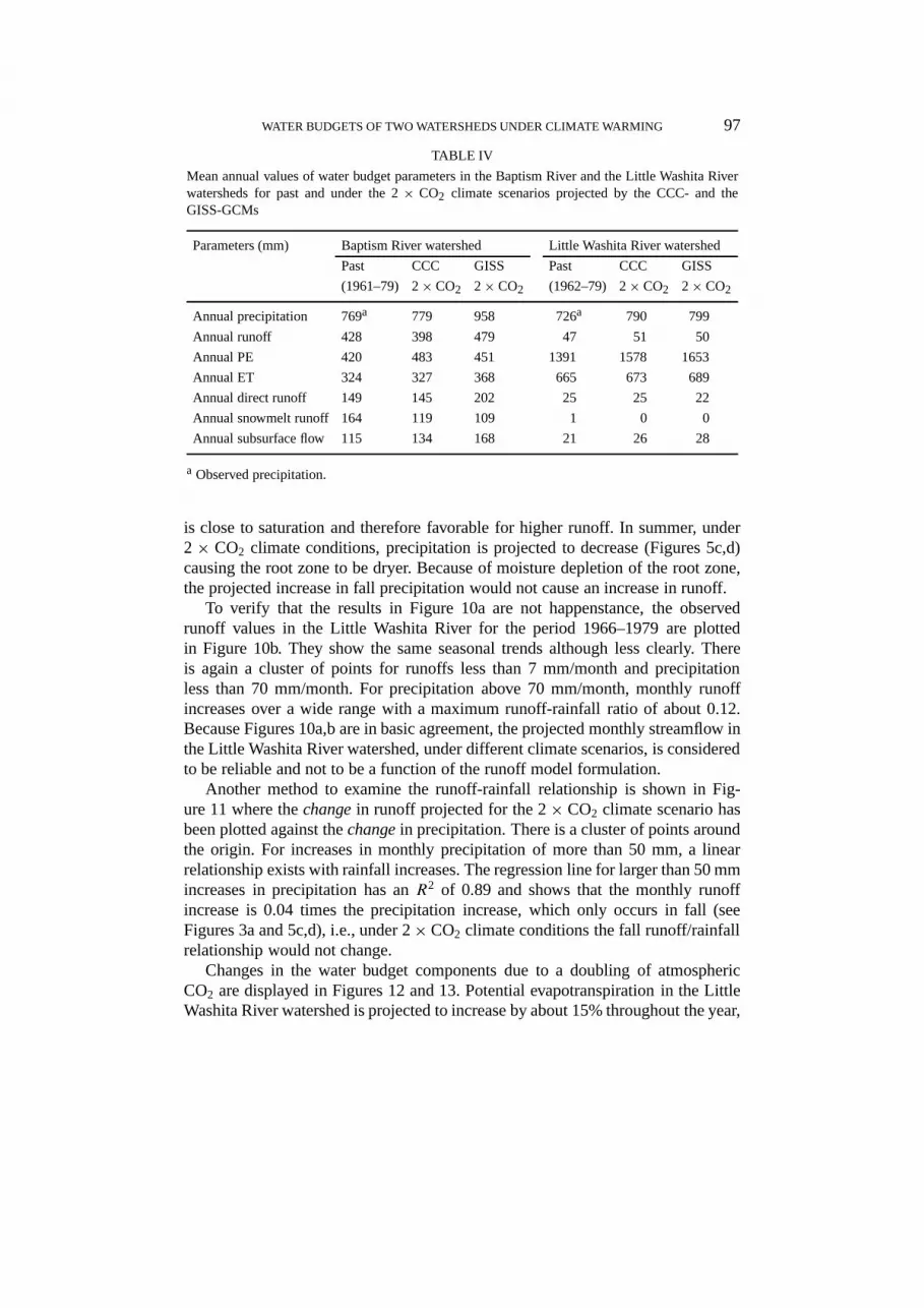
TABLE IV

Mean annual values of water budget parameters in the Baptism River and the Little Washita Riverwatersheds for past and under the 2× CO2 climate scenarios projected by the CCC- and theGISS-GCMs

Parameters (mm) Baptism River watershed Little Washita River watershed

Past CCC GISS Past CCC GISS

(1961–79) 2× CO2 2× CO2 (1962–79) 2× CO2 2× CO2

Annual precipitation 769a 779 958 726a 790 799

Annual runoff 428 398 479 47 51 50

Annual PE 420 483 451 1391 1578 1653

Annual ET 324 327 368 665 673 689

Annual direct runoff 149 145 202 25 25 22

Annual snowmelt runoff 164 119 109 1 0 0

Annual subsurface flow 115 134 168 21 26 28

a Observed precipitation.

is close to saturation and therefore favorable for higher runoff. In summer, under2× CO2 climate conditions, precipitation is projected to decrease (Figures 5c,d)causing the root zone to be dryer. Because of moisture depletion of the root zone,the projected increase in fall precipitation would not cause an increase in runoff.

To verify that the results in Figure 10a are not happenstance, the observedrunoff values in the Little Washita River for the period 1966–1979 are plottedin Figure 10b. They show the same seasonal trends although less clearly. Thereis again a cluster of points for runoffs less than 7 mm/month and precipitationless than 70 mm/month. For precipitation above 70 mm/month, monthly runoffincreases over a wide range with a maximum runoff-rainfall ratio of about 0.12.Because Figures 10a,b are in basic agreement, the projected monthly streamflow inthe Little Washita River watershed, under different climate scenarios, is consideredto be reliable and not to be a function of the runoff model formulation.

Another method to examine the runoff-rainfall relationship is shown in Fig-ure 11 where thechangein runoff projected for the 2× CO2 climate scenario hasbeen plotted against thechangein precipitation. There is a cluster of points aroundthe origin. For increases in monthly precipitation of more than 50 mm, a linearrelationship exists with rainfall increases. The regression line for larger than 50 mmincreases in precipitation has anR2 of 0.89 and shows that the monthly runoffincrease is 0.04 times the precipitation increase, which only occurs in fall (seeFigures 3a and 5c,d), i.e., under 2×CO2 climate conditions the fall runoff/rainfallrelationship would not change.

Changes in the water budget components due to a doubling of atmosphericCO2 are displayed in Figures 12 and 13. Potential evapotranspiration in the LittleWashita River watershed is projected to increase by about 15% throughout the year,


Figure 11.Monthly changes in simulated runoff versus monthly changes in precipitation in the LittleWashita River.

under both 2×CO2 climate scenarios (Figure 12b). However, little change in actualevapotranspiration is projected for most months (Figure 12c) except July (becauseof less rainfall in summer, Figures 5c,d) and October (because of more rainfallin fall). The associated simulated moisture content of the root zone is projected todecrease by about 20 mm in June and July (Figure 13a) under both 2×CO2 climatescenarios. Similarly, SBR is projected to increase in winter, and to drain until latespring (Figure 13b).

The monthly runoff components of the Little Washita River are shown in Fig-ure 14. A significant decrease in direct runoff is projected in June and July, and asignificant increase in September or October under both climate scenarios. Morethan 20% increase in subsurface flow is projected from fall to winter due to asignificant rainfall increase in fall.

8. Discussion

The relationship between the water budget and the climate change in two smallwatersheds of the central U.S. was investigated. One (Baptism River) is a forestedwatershed located in northern Minnesota in the drainage basin of Lake Superior, inthe temperate zone with seasonally cold climate. Mean annual runoff is 428 mm or


Figure 12. Mean monthly potential and actual evapotranspiration in the Little Washita Riverwatershed simulated for past and 2× CO2 climate scenarios.


Figure 13.Mean monthly water storage components in the Little Washita River watershed simulatedfor past and 2× CO2 climate scenarios.

56% of mean annual precipitation (769 mm). The other watershed (Little WashitaRiver) is an agricultural watershed in southwestern Oklahoma, in the drainagebasin of the Red River, in a warm climate. Mean annual runoff is only 47 mm or7% of mean annual precipitation (726 mm). The water budget components are verydifferent in the two watersheds. Despite similar annual precipitation, annual runoffvalues are an order of magnitude different. Annual evapotranspiration from thenorthern watershed is less than 50% of that from the southern watershed (Table IV).

A deterministic runoff model was used to estimate monthly runoff from threecomponents: Direct runoff, subsurface flow (interflow and base flow) and snow-melt. Direct runoff in the northern watershed is 35% (149 mm) and in the southern


Figure 14. Mean monthly runoff components in the Little Washita River simulated for past and2× CO2 climate scenarios.

watershed 53% (25 mm) of the annual runoff (Table IV). Subsurface flow is 27%(115 mm) and 45% (21 mm) in the northern and southern watersheds, respectively.The northern watershed has significant water storage as snow in winter and heavysnowmelt runoff (38% of the annual runoff) in spring. The southern watershed hasno snowmelt runoff.

After the model was calibrated, climate conditions of the past and climate con-ditions projected by two GCMs (GISS and CCC) for a 2× CO2 climate conditionwere applied to the model. All watershed characteristics in the model were assumedto remain the same, i.e., no changes in vegetation cover were imposed. The twoGCMs indicate different climate change scenarios for 2×CO2 climate conditions;


the differences are more pronounced for the Baptism River watershed than forthe Little Washita River watershed. The two watersheds, of similar size and withabout the same annual precipitation are projected to have different responses partlybecause they are located in different climate regions. The Baptism River will likelyrespond with an increase in winter runoff and a decrease in spring runoff withrespect to the past, whereas the Little Washita River will likely respond with anincrease in fall and winter runoff and a decrease in summer runoff. No significantchange in mean annual runoff is projected for the Baptism River and only a 7%increase in mean annual runoff is projected for the Little Washita River. Evapotran-spiration, soil moisture content and direct runoff are projected to decrease in midsummer and to increase in fall in the Little Washita River watershed with respect tothe past whereas no definite change in these parameters is projected in the BaptismRiver watershed. Interestingly, a 35% increase in August precipitation (90 mm) inthe Baptism River watershed (projected by the GISS-GCM) causes a significantincrease in the moisture content of the root zone, an increase in actual evapo-transpiration and direct runoff; however, a 40% increase in August precipitation(65 mm) in the Little Washita River watershed (projected by the GISS-GCM) givesno significant increase in the moisture content of the root zone, and no significantchange in actual evapotranspiration and direct runoff. Under both 2×CO2 climatescenarios, SBR and subsurface flow are projected to increase in fall, winter andspring in both watersheds. This is also the cause for about 20% increase in winterrunoff.

9. Summary

Under 2× CO2 climate scenarios, snowmelt runoff in the northern watershed isprojected to start earlier and to be smaller than in the past. The shallow aquifer isrecharged earlier in spring, and more subsurface flow is projected in fall, winterand spring. In months where precipitation is rainfall, if rainfall is more than 70mm/month, then the projected monthly runoff change is about one half the changein the monthly rainfall. No significant change in annual runoff is projected for theBaptism River.

For the southern watershed, precipitation is forecast to decrease in summerand to increase in fall. Runoff projections are also consistent with the rainfall, asmall (less than 25%) decrease in June and July runoff and a substantial (50–80%)increase in early fall. Because the main projected increase in precipitation occurs infall, when surface soil is at its driest condition, the projected direct runoff increaseis only 4% of the change in monthly precipitation. This absorption of additionalprecipitation by the soil is also consistent with a projected decrease in soil moistureof about 20% in June and July under the 2×CO2 climate conditions. On an annualbasis, about 7% increase in runoff is projected for the Little Washita River underboth climate scenarios.


The two watersheds respond differently to 2×CO2 climate conditions. The onlycommon point between the two watersheds is an increase in winter runoff whichis in agreement with findings by Gleick (1987b), Lettenmaier et al. (1990) andNewman et al. (1992).

The monthly/seasonal changes in climate variables play a crucial role ineach watershed’s runoff response to precipitation. Hence a reliable projection ofmonthly climate conditions by GCMs will give more realistic results for runoffthan annual climate scenarios. The runoff model used follows the main hydrolo-gic processes and can be considered a meaningful tool for runoff projections inresponse to climate changes. Further improvements in runoff projections wouldrequire adjustments in runoff process time scales, potential changes in vegetationcover in the watershed and more reliable 2×CO2 climate predictions from GCMs.

Acknowledgements

The work reported herein was supported by the National Water Quality Laboratory,Agricultural Research Service/USDA in Durant, Oklahoma and the Mid-ContinentEcology Division, U.S. Environmental Protection Agency, Duluth, Minnesota. Drs.Robert Williams, and John Eaton/Virginia Snarski were project officers.

References

Allen, P. B. and Naney, J. W.: 1991,Hydrology of the Little Washita River Watershed, Oklahoma;Data and Analysis, U.S. Department of Agriculture, Agricultural Research Service, Durant, OK,ARS-90.

Giorgi, F., Brodeur, C. S., and Bates, G. T.: 1994, ‘Regional Climate Change Scenarios over theUnited States Produced with a Nested Regional Climate Model’,J. Climate7, 375–399.

Giorgi, F., Meehl, G. A., Kattenberg, A., Grassl, H., Mitchell, J. F. B., Stouffer, R. J., Tokioka, T.,Weaver, A. J., and Wigley, T. M. L.: 1998, ‘Simulation of Regional Climate Change with GlobalCoupled Climate Models and Regional Modeling Techniques’, in Watson, R. T., Zinyowera,M. C., and Moss, R. H. (eds.),The Regional Impacts of Climate Change, Cambridge UniversityPress, Cambridge, U.K.

Gleick, P. H.: 1987a, ‘The Development and Testing of a Water Balance Model for Climate ImpactsAssessment: Modeling the Sacramento Basin’,Water Resour. Res.23, 1049–1061.

Gleick, P. H.: 1987b, ‘Regional Hydrologic Consequences of Increases in Atmospheric CO2 andOther Trace Gases’,Clim. Change10, 137–160.

Hansen, J., Russell, G., Rind, D., Stone, P., Lacis, A., Lebedeff, S., Ruedy, R., and Travis, L.: 1983,‘Efficient Three-Dimensional Global Models for Climate Studies: Model I and II’,Mon. Wea.Rev.111, 609–662.

Hostetler, S. W. and Giorgi, F.: 1995, ‘Effects of 2× CO2 Climate on Two Large Lake Systems:Pyramid Lake, Nevada, and Yellowstone Lake, Wyoming’,Global Planet. Change10, 43–54.

Hughes, J. P. and Guttorp, P.: 1994, ‘A Class of Stochastic Models for Relating Synoptic AtmosphericPatterns to Regional Hydrologic Phenomena’,Water Resour. Res.30, 1535–1546.

Lettenmaier, D. P. and Gan, T. Y.: 1990, ‘Hydrologic Sensitivity of the Sacramento–San JoaquinRiver Basin, California, to Global Warming’,Water Resour. Res.26, 69–86.


McCabe Jr., G. J. and Ayers, M. A.: 1989, ‘Hydrologic Effects of Climate Change in the DelawareRiver Basin’,Water Resour. Bull.25, 1231–1242.

McFarlane, N. A., Boer, G. J., Blanchet, J. P., and Lazare, M.: 1992, ‘The Canadian Climate CenterSecond-Generation General Circulation Model and its Equilibrium Climate’,J. Climate5.

Mimikou, M., Kouvpoulos, Y., Cavadias, G., and Vayianos, N.: 1991, ‘Regional Hydrological Effectsof Climate Change’,J. Hydrol.123, 119–146.

Mohseni, O. and Stefan, H. G.: 1998, ‘A Monthly Streamflow Model’,Water Resour. Res.34, 1287–1298.

National Research Council: 1982,Carbon Dioxide/Climate Review Panel. Carbon Dioxide andClimate: A Second Assessment, National Academy Press, Washington, D.C.

National Research Council: 1983,Changing Climate: Report of the Carbon Dioxide AssessmentCommittee, National Academy Press, Washington, D.C.

Newman, L. E., Baker, D. G., and Skaggs, R. H.: 1992,The Effects of Climate Variability and Green-house Effect-Scenarios on Minnesota’s Water Resources, Technical Report No. 135, Universityof Minnesota, Department of Geography and Soil Sciences, Water Resources Research Center.

Rao, A. R. and Al Wagdany, A.: 1995, ‘Effects of Climate Change in the Wabash River Basin’,J.Irrigation Drainage Engng.121, 207–215.

Russell, L. G., Miller, J. R., and Rind, D.: 1995, ‘A Coupled Atmosphere-Ocean Model for TransientClimate Change Studies’,Atmos.-Ocean33, 683–730.

Schaake Jr., J. C.: 1990, ‘Climate Change’, in Waggoner, P. E. (ed.),Climate Change and U.S. WaterResources, Wiley, New York.

Shaw, E. M.: 1983,Hydrology in Practice, 2nd edn., Chapman and Hall, London.Singh, P. and Kumar, N.: 1997, ‘Impact Assessment of Climate Change on the Hydrological Re-

sponse of a Snow and a Glacier Melt Runoff Dominated Himalayan River’,J. Hydrol. 193,316–350.

Sorooshian, S. and Gupta, V. K.: 1983, ‘Automatic Calibration of Conceptual Rainfall-RunoffModels: The Question of Parameter Observability and Uniqueness’,Water Resour. Res.19:260–268.

Thornthwaite C. W. and Mather, J. R.: 1955, ‘The Water Balance’, inPublications in ClimatologyLaboratory of Climatology, 8(1).

U.S. Army Corps of Engineers: 1956,Summary Report of the Snow Investigations: Snow Hydrology,Report, North Pacific Division, Portland, OR.

van Hylckama, T. E. A.: 1956, ‘The Water Balance of the Earth’,Publications in Climatology,Laboratory of Climatology, 9(2).

von Storch, H., Zorita, E., and Cubasch, U.: 1993, ‘Downscaling of Global Climate Change Estimatesto Regional Scales: An Application to Iberian Rainfall in Wintertime’,J. Climate6, 1161–1171.

Wilks, S. D.: 1992, ‘Adapting Stochastic Weather Generation Algorithms for Climate ChangeStudies’,Clim. Change22, 67–84.

Xu, C. Y. and Halldin, S.: 1997, ‘The Effect of Climate Change on River Flow and Snow Cover inthe NOPEX Area Simulated by a Simple Water Balance Model’,Nordic Hydrol.28, 273–282.

Zorita, E., Hughes, J. P., Lettenmaier, D. P., and von Storch, H.: 1995, ‘Stochastic Characterizationof Regional Patterns for Climate Model Diagnosis and Estimation of Local Precipitation’,J.Climate8, 1023–1042.

(Received 10 February 1999; in revised form 7 June 2000)

water budgets of two watersheds in different climatic zones under projected climate warming

Documents