Wage Subsidies and Skill Formation: A Study of the Earned Income Tax

Credit

Ricardo Cossa�

James J. Heckman��

Lance Lochner���

First Draft, November, 1997

This Version, May 1999

�University of Chicago, Department of Economics. ��University of Chicago, Department

of Economics and The American Bar Foundation. ���University of Rochester, Department

of Economics. This research was sponsored by NSF-97-09-873 and a grant from the Ameri-

can Bar Foundation. This paper was presented at a conference on wage subsidies sponsored

by the Russell Sage Foundation in New York, December, 1997, IRP conference at the Uni-

versity of Wisconsin, June, 1998, at the Western Economics Association Meeting, July,

1998, at the University of Rochester, November 1998, and at a Public Sector Workshop at

the University of Chicago, May 1999. We thank Alejandra Cox Edwards, Larry Summers,

Edmund Phelps and especially Casey Mulligan and Yona Rubenstein for comments on this

paper.

1 Introduction

Recent calls for wage subsidies have emphasized their value for attaching low skill persons

to the workplace. Firms o�ered compensation for hiring low skill workers will employ more

of them and attract them away from lives of idleness or crime. Wage subsidies can undo

the disemployment e�ects of minimum wage laws and welfare programs (Phelps, 1997;

Heckman, Lochner, Smith, and Taber, 1997; and Lochner, 1998).

Previous research on wage subsidies has focused exclusively on the e�ect of such subsidies

on employment and labor supply. This paper examines the impact of wage subsidies on the

skill formation of the subsidized. By promoting work among those who would not otherwise

work, wage subsidies create incentives for workers to invest in skills that are useful in the

workplace.

The skill formation e�ects of wage subsidies on persons who would work without the

subsidy are more subtle. If skills are acquired as a by-product of work (learning-by-doing),

wage subsidies will encourage skill acquisition if workers increase their labor supply in

response to the subsidy. If learning is rivalrous with working as in Becker (1964) or Ben

Porath (1967), wage subsidies can discourage investment in skills.

In addition to these e�ects, there is an even more subtle e�ect of wage subsidies on

skill formation arising from the nonlinearity in the return to work created by many pro-

posed schemes. These nonlinearities arise from the targeted nature of most programs. For

speci�city, consider the Earned Income Tax Credit program (EITC), a major wage subsidy

program in the U.S. that we study in this paper.1 Figure 1 graphs the EITC supplement

to annual labor earnings as a function of labor earnings for a prototypical person. For ana-

lytical simplicity, we abstract from all other tax-transfer programs or else assume that they

generate proportional schedules that preserve Figure 1 as a key feature of the budget set

facing workers. Whether or not this is true is an open empirical question. In the �rst region

of Figure 1, [0; a), the hourly wage is subsidized. In the second region, [a; b), the hourly

wage is the pre-subsidy wage, but the worker's total income is increased by the amount of

the annual subsidy, Sb. In the third region, [b; c), the subsidy is phased out and the e�ective

hourly wage is below the pre-subsidy wage level because each hour worked eliminates part

of the subsidy. When earnings are su�ciently high, (at or above c), the e�ective wage is

again the pre-subsidy wage. What is the e�ect of this subsidy scheme on skill formation?

In the standard economic model of skill formation, the major cost of skill investment

1Strictly speaking, the EITC subsidizes wage earnings rather than wage rates. For a given pre-subsidywage, the EITC alters the post-subsidy wage received for each hour worked and is e�ectively a wage subsidy.

1

is foregone earnings. Assume for simplicity that these are the only costs. In particular,

suppose for now, as in Becker (1964) and Ben Porath (1967), that we ignore the leisure costs

of investment. Time is devoted either to work or investment and people seek to maximize

the present value of their earnings. By abstracting from the labor-leisure decision that

motivated the introduction of the EITC, we can focus on the main impact of the program on

skill investment among workers without worrying about the e�ect of income ows generated

by the program on the total level of labor supplied to the market.

Suppose, for simplicity, that skills do not depreciate. In this case, wages always rise

(or remain constant) as investment is made over the life cycle. To simplify the argument

further, ignore any general equilibrium factor price e�ects arising from changes in aggregate

skill levels induced by the program.

For a person starting life on the �rst segment of the EITC schedule, the opportunity

cost of time investing in skill is raised compared to what it would be in the absence of the

program. If the investment produces su�cient earnings growth so that persons eventually

leave the �rst segment as their skills are enhanced, the e�ect of the subsidy is to reduce

skill formation, because the opportunity cost of time spent investing is increased during the

years when investment is made but the wage payment per hour of work is not increased

during the payo� years. Only if a person stays on the �rst segment throughout his working

lifetime will the e�ect of the subsidy be neutral on skill formation. In this case, marginal

returns and costs rise in the same proportion and there is no e�ect on skill investment.

For a person who starts life on the at segment of the subsidy schedule, the e�ects of

the subsidy on investment are ambiguous. First, if a person has annual earnings that never

leave the at segment, there is no e�ect of the subsidy on skill formation, since there is no

marginal e�ect of the program on either returns or costs. (Recall that there are no wealth

e�ects.) Second, if earnings rise so that the person spends part of his or her career on the

declining segment, skill formation is retarded, because the payo� to investment in human

capital is reduced as the subsidy is withdrawn. If a person jumps from the at segment to

a post-program earnings level above c, there again would be no e�ect of the program on

skill formation, although the continuous nature of the skill formation process makes this

case an empirically unlikely one.

Finally, consider a person who starts out life with initial earnings on the third (declining

subsidy) segment. In this case, the tax on earnings implicit in this schedule makes invest-

ment less costly compared to a no-program world, since earnings foregone are lowered by

the subsidy. If investment eventually causes the person to leave the third segment, the tax

2

on earnings is eventually removed and, hence, the relative payo� to investment is increased

by the subsidy. This e�ect promotes skill formation.

The overall e�ect of the program on the skill formation of workers a�ected by the

program is ambiguous even in this simple model. It can only be determined by an empirical

analysis. Adding the labor-leisure choice further complicates matters. The wealth e�ects

of the subsidy serve to reduce labor supply and, hence, the incentive to acquire skills.

Wage e�ects are ambiguous, depending on the relative strengths of income and substitution

e�ects. When substitution e�ects dominate, the EITC encourages skill investment for

individuals who spend their entire careers in the phase-in region or for those who move

from the phase-out region o� the schedule. Finally, the EITC may draw people into the

workplace. This will increase their hours of work and will increase their incentive to invest

in work-related skills.

Persons may also be drawn into the workforce by the EITC when skills are acquired

through work experience rather than through a separate learning activity as in the Becker

- Ben Porath model. In the conventional learning-by-doing model, investment time and

work time are the same, and the activity of investment is not rivalrous with earning. In

this framework, the e�ects of the EITC on skills accumulated through learning-by-doing

are much di�erent than they are in the Becker - Ben Porath model for persons who would

work even in its absence. For them, skill accumulation depends only on labor supply, so

for workers induced to work more hours, the EITC raises skills. Those induced to work

less by the program accumulate fewer skills. The EITC only raises hours worked among

workers whose earnings lie in the phase-in region of the schedule, assuming substitution

e�ects dominate income e�ects in determining labor supply. For all other workers, the

EITC reduces hours worked and, therefore, skills acquired through learning-by-doing. The

contrast between the e�ects of wage subsidies on skill formation in a learning-by-doing

model and in a Becker - Ben Porath model is a major �nding of this paper.

Our exposition proceeds in the following way. An analysis of the e�ect of the EITC

program on skill investment involves many issues: the choice of a model of skill formation

and labor supply, modi�cations for credit constraints and the like. To take these models to

data, it is necessary to develop multiperiod versions of models of skill formation and labor

supply. In addition, the reward function based on a schedule like that displayed in Figure 1

is non-di�erentiable and non-concave in control variables, at least for certain con�gurations

of parameter values.

In order to clarify the essential features of the program, we initially simplify the analysis.

3

In Section 2, we use a two period model of skill formation to analyze the e�ects of age-

speci�c, proportional wage subsidies or wage taxes on skill investment for several types

of subsidy programs using the two competing models of skill formation. At any age, we

assume that taxes or subsidies are the same irrespective of earnings levels, contrary to the

actual features of the EITC as depicted in Figure 1. Thus, we initially abstract from non-

concavity of the criterion and nonuniqueness in investment induced by the EITC schedule.

We explicitly account for these features in a later section. In this simpli�ed model, we can

focus attention on the primary incentives in tax-subsidy programs without getting bogged

down in details.

We establish that the two main models of skill formation widely used in the literature,

the Becker - Ben Porath model and a learning-by-doing model, have di�erent implications

for the e�ect of wage subsidies on skill formation. When the conventional learning-by-doing

model is carefully examined, it contains an apparent \free lunch" feature { persons who

work also acquire skill. The more they work, the more skills they acquire, so no earnings are

foregone. Foregone leisure is the sole cost of investment in this model. When a market for

jobs with di�erent learning content is introduced following Rosen (1972), earnings foregone

are added as a cost of acquiring skills in a learning-by-doing model and a major source of

disagreement between the two models of skill formation is eliminated. In a special case

which we establish below, the two models become e�ectively equivalent if leisure is added

to the Becker - Ben Porath framework, and if learning-by-doing opportunities are priced

appropriately.

In Section 3, we discuss speci�c features of the EITC program. We extend the models of

age-speci�c wage subsidies to consider the actual wage subsidies implicit in the EITC pro-

gram, which depend on the level of earnings. We discuss the resulting non-di�erentiability

and non-concavity of the criterion function for certain parameter con�gurations and the

need to account for a multiplicity of local optima in estimating the impact of the EITC

program and simulating its impact.

We present an analysis of the distribution of various demographic groups over the four

segments of Figure 1. We show that for most low skill working groups, the empirically

important range extends over segments three and four (segments [b; c) and [c;1) in that

�gure). The tax on earnings over segment [b; c) encourages investment among workers in

the standard model of investment if those workers eventually earn above c. In addition, the

EITC program stimulates work among non-workers and, thus, stimulates their investment

in human capital.

4

Section 4 extends the analysis of Section 3 to a multiperiod setting. The intuitions

developed in the simple two period models apply more generally. Section 5 presents es-

timates of two canonical models of skill formation using CPS data on wages and hours

worked for di�erent demographic groups. Our evidence suggests that a learning-by-doing

model is more consistent with the data than the conventional Becker - Ben Porath model

of on-the-job training.

Section 6 examines the implications of the two di�erent models of skill formation for

the impact of the EITC program on earnings and wage growth. Both models produce

approximately the same estimates of EITC-induced entry into the work force on wage

growth and human capital accumulation. The models di�er greatly in their prediction of

the quantitative impact of the EITC program on the wage growth of those who would work

even in the absence of the EITC program. Qualitatively, the models agree. Both predict

declines in potential skill levels over the empirically relevant range for most demographic

groups. But the predicted declines are quantitatively greater in the Becker - Ben Porath

model than they are in a conventional learning-by-doing model. For some educated males,

however, the Becker - Ben Porath model predicts increases in skills, since they move from

the phase-out region to beyond the maximum qualifying amount (c).

The learning-by-doing model predicts substantially larger negative impacts of the EITC

on hours worked. As a result, it also predicts larger declines in earnings than the OJT

model. If the entry e�ects of the EITC are small, the reductions in earnings can be as

large as 7% of the average skill level supplied to the market. While the aggregate e�ects

of the EITC on skills are similar in the two models, the predicted impacts on speci�c

groups of workers are often quite di�erent. Average measures of the impact of the EITC on

skills mask considerable heterogeneity in individual responses. These �ndings highlight the

importance of determining the appropriate model of skill formation in assessing the impact

of the EITC program on the skills and earnings of workers.

2 Models of Wage Subsidies and Skill Formation

This section analyzes several two period models of skill accumulation to investigate the

e�ect of proportional wage subsidies on skill formation. The EITC is not a period-speci�c

proportional wage subsidy. But the intuition obtained from an analysis of the simple

period-speci�c proportional subsidy and tax case carries over to the more general EITC

structure. We consider both income maximizing models and models with labor supply

assuming perfect credit markets. We also consider a version of the labor supply model with

5

borrowing constraints. Throughout this paper, we ignore the practically important issues

of fraud and enforcement in the administration of wage subsidy programs that are discussed

by Phelps (1997). In this paper, we focus on subsidies and taxes to workers based on their

hourly wages. Absent any frictions in the labor market such as minimum wages, a tax or

subsidy to �rms based on the hourly wage paid to workers has equivalent e�ects on hours

worked, the net wage paid to workers and their investment.2 Thus our analysis applies to

hourly wage subsidies to �rms or to workers.

Central to this investigation is the speci�cation of the skill formation process and the

costs of skill formation. The conventional model, due to Becker (1964) and Ben Porath

(1967), features earnings foregone as the main cost of skill formation. In this model, a

wage subsidy in the �rst period of a two period model tends to divert workers away from

investment and toward market work. Wage subsidies tend to reduce skill formation.

However, there is another model of skill formation that produces some diametrically

opposite conclusions: a model of learning-by-doing as developed by Heckman (1971), Weiss

(1972), Killingsworth (1982), Shaw (1989) and Altug and Miller (1990 and 1998). In this

model, an hour of work at any job produces skill (learning-by-doing) that has the same

value in all sectors of the economy. A wage subsidy that promotes work in the �rst period

promotes skill formation. The cost of work and skill acquisition in the learning-by-doing

model is leisure foregone.

This second model of skill formation appears to have a free lunch aspect to it. People

who work more in the �rst period have higher earnings both in the �rst and the second

period. There is no tradeo� between skill formation and earnings from work as in the

Becker - Ben Porath model. There is still a tradeo� between leisure and acquiring skills

through work, so in truth, there is no free lunch.

What produces the apparent free lunch is the implicit assumption that for any worker

an hour of work in any job is equally e�ective in producing skill. If jobs di�er in the rate

at which an hour of work produces skill, a market for jobs arises that is usually ignored in

analyses of learning-by-doing models. All current workers who will also work in the future

will cluster in the jobs with the highest learning content unless those jobs command higher

prices. Higher prices for jobs with more training content mean lower �rst period wages

for such jobs if workers of the same skill level and tastes have choices among otherwise

2In the presence of a minimum wage, a subsidy per worker-hour employed by the �rm can have di�erente�ects than a subsidy to the worker if the minimum wage is binding, because the wage of the worker willnot be able to adjust downward to accomodate the induced increase in supply. In this case, subsidies to�rms will be more e�ective.

6

equal jobs with di�erent training content.3 With the addition of heterogeneity in learning

opportunities, and prices of those opportunities, we regain a tradeo� between �rst period

investment and earnings from work.

2.1 Speci�cations of Skill Formation Equations

The most commonly used speci�cation of the human capital accumulation process is due

to Ben Porath (1967). Human capital in period 1, H1; is produced by time investment I.

(We assume there is no depreciation, so human capital is non-decreasing.) Thus, we write

(1) H1 �H0 = F (I)

with F 0 > 0, F 00 < 0, 0 � I � 1, where I is the e�ective proportion of time spent investing,

and H0 is the initial stock of human capital.

Assuming a perfect capital market with interest rate r and an e�ciency units model of

labor services with price R per e�ciency unit, agents choose I to maximize

(2) RH0(1� I) +R

1 + rH1

subject to (1). Investment is rivalrous with earnings. This formulation recognizes that there

will be no investment in the second (and �nal) period of life. We only consider the problem

for a single individual or a small set of individuals and ignore any general equilibrium e�ects

on factor prices.

Optimality requires that

(3) RH0 �R

1 + rF 0(I):

If I 6= 1, we are certain to obtain an interior solution provided F 0(0) = 1. Changes in R

do not a�ect skill investment. Increases in r decrease investment; so does an increase in

H0. The higher the �rst period opportunity wage or the lower the discounted return from

investment, the less time is spent investing.4

A proportional wage subsidy of (1 + �) per period clearly does not a�ect investment.

A wage subsidy of �0 in the �rst period, followed by �1 in the second, changes the interior

solution �rst order condition to

(4) (1 + �0)RH0 = (1 + �1)R

1 + rF 0(I):

If �0 > �1; investment is reduced compared to the case where �0 = �1; if �0 < �1, then

investment is increased.

We return to this model and analyze it more thoroughly after we develop a comparison

model of learning-by-doing. For that model, skills are produced by work. Let Lt be leisure

3Rosen (1972) introduced the notion of a market for jobs with di�erent training/learning content.4In the case of a strict inequality for (3), we obtain the stated results as \tendencies" i.e. predicted

increases in investment become predicted non-decreases.

7

in period t. There is no investment time, per se, so hours of work are given by 1 � Lt. In

this scheme

(5) H1 �H0 = '(1� L0)

with '0 > 0, '00 < 0. In principle, work in the second period also produces human capital,

but that output is not valued since there is no third period in the model. The cost of

work and acquiring new skills is leisure foregone. To introduce such costs, it is necessary

to introduce a utility function to value leisure. Then the consumer's problem is to choose

consumption and leisure to

(6) Max U(C0; L0) +1

1 + �U(C1; L1)

(where U is strictly concave and � is a discount factor) subject to

(7) RH0[1� L0](1 + �0) +R

1 + rH1[1� L1](1 + �1) +A0 = C0 +

C1

1 + rand (5) where A0 represents initial assets. Throughout this paper, we assume that goods

and leisure are normal. Let � denote the LaGrange multiplier associated with (7). Assuming

an interior solution, we obtain the following �rst order conditions:

(8a) U1(C0; L0) = �

(8b) U1(C1; L1) = �

�1 + �

1 + r

�

(8c) U2(C0; L0) = �R

�H0(1 + �0) +

'0(1� L0)[1� L1](1 + �1)

1 + r

�

(8d) U2(C1; L1) = �

�1 + �

1 + r

�R(H0 + '(1� L0))(1 + �1):

The price of time in the �rst period is potential earnings (RH0(1+� 0)) plus the e�ect of

an extra unit of work on discounted future earnings (R'0(1�L0)[1 �L1])(1+� 1)=(1+r)): As

�rst noted by Heckman (1971), even when � = r, it is possible that wages grow between pe-

riods 0 and l, but labor supply is the same in both periods even if labor supply increases with

the price of time. The opportunity cost of leisure

�RH0(1 + �0) +

R'0(1� L0)[1� L1](1 + �1)

1 + r

�in period 0 can equal the realized wage in period 1 (RH0 +R'(1� L0)(1 + � 1)).

In this model, an increase in R produces income and substitution e�ects. Compensating

to eliminate income e�ects, an increase in R promotes skill formation and labor supply.

There is no tradeo� between investment and work, because work is investment. If wages

are subsidized (�0 > 0) in period 0 and taxed (�1 < 0) in period 1 and the consumer is

compensated to eliminate income e�ects, the e�ects on skill formation are ambiguous: the

�rst period wage, RH0(1+ � 0), is increased but the future return,R'0(1� L0)[1� L1]

1 + r(1+

�1), is diminished.

In contrast to the model of skill investment previously analyzed, a compensated wage

subsidy in period zero that is changed to a wage tax in period one has ambiguous e�ects.

8

It may increase skills if the positive e�ects on current returns more than o�set the negative

e�ects on future returns. Similarly, a compensated wage tax applied in period zero followed

by a wage subsidy in period one also has ambiguous e�ects on skills. The resulting increase

in the return on future work may promote work (and, hence, investment) in the �rst period.

If �1 = 0, a wage subsidy in period 0 (�0 > 0) promotes skill formation, while a wage

tax (� 0 < 0) lowers skills { exactly the opposite from what is predicted in the Becker

- Ben Porath investment framework. These di�erences can be tested econometrically to

distinguish between the two models of skill formation.

2.2 Reconciling the Two Models of Skill Formation

The two models just considered have di�erent predictions about the e�ects of simple tax

and subsidy schemes on skill formation. What is the source of this di�erence? We now show

that adding leisure to the �rst model does not change the qualitative predictions derived

from it, provided that we compensate for income e�ects and provided that solutions are

interior. Allowing di�erent jobs to have di�erent training content, and pricing out the

training, moves the two models together.

As above, we write lifetime utility in terms of concave utility functions and the rate of

time preference �:

U(C0; L0) +1

1 + �U(C1; L1):

The utility function is maximized subject to

RH0[1� I � L0](1 + �0) +R

1 + r[F (I) +H0][1� L1](1 + �1) +A0 = C0 +

C1

1 + r:

This expression incorporates the observation that at the end of life there is no investment

I: As long as the agent works in period zero, a compensated wage subsidy in period zero

raises the price of time and reduces investment and leisure.

The interior solution �rst order conditions for leisure and investment are

(9a) U2(C0; L0) = �RH0(1 + �0)

(9b) U2(C1; L1) = �R[H0 + F (I)]

�1 + �

1 + r

�(1 + �1)

(10)R

1 + rF 0(I)[1 � L1](1 + �1) = RH0(1 + �0):

In this extended Becker - Ben Porath model, changes in R are no longer neutral. Holding

wealth e�ects constant, an increase in R increases skill formation by encouraging labor

supply in period 1. The qualitative e�ects of changes in taxes and subsidies in periods

0 and 1 are the same as in the income maximizing version of this model. If �0 < 0 and

�1 > 0, skill accumulation is fostered compared to the case where �0 = �1 = 0. If �0 > 0

9

and �1 < 0, skill accumulation is dampened. Adding leisure but compensating for wealth

e�ects, we obtain the same predictions about the impact of period-speci�c wage subsidies

on investment as is produced in the original Becker - Ben Porath model.

The crucial economic di�erence between the Becker - Ben Porath model and the learning-

by-doing model of skill formation is not that one model excludes leisure while the other

includes it. The major source of the di�erence is that in the Becker - Ben Porath model,

investment and labor supply compete for the agent's time budget while in the learning-

by-doing model they do not. In the Becker - Ben Porath model, higher investment comes

at the cost of foregone earnings. In the conventional learning-by-doing model, work and

investment are the same activity. A worker receives more current and future earnings by

working more today. There is no cost of foregone earnings for investment. The only cost is

foregone leisure.

Now consider a di�erent case where �rms di�er in the rate at which workers can learn

from an hour of work. All workers who plan to work in period 1 would ock to the �rms

that o�ered the highest total earnings package inclusive of future earnings. If �rms pay

the same spot wage R for H0, the �rm with the higher learning potential would attract all

the workers. Only workers who did not plan to work in period 1 would ignore the training

potential of a prospective job. Those who plan to work a lot would value it highly. In

the �nal period of our two period model, however, workers would not value jobs with high

training content, because they will not be able to harvest the fruits of their investment.

Everything else the same, older workers would prefer jobs with no training content.

To investigate this model more systematically, let � index the investment content of a

job, so we write the learning-by-doing function as '(1� L0; �): Assume

@2'

@�@(1� L0)> 0;

so opportunities with higher � produce greater learning-by-doing per hour of work. Assume

further that '(0; �) = 0, for all �, so that a person must work in order to harvest the bene�t

of �. For the same wage RH0, workers would prefer to work in �rms with higher �. Only

persons who choose not to work in period one are unconcerned about the � content of their

job. Implicit in the learning-by-doing speci�cations used in the literature is the assumption

that all �rms provide the same learning opportunities { i.e. � is identical across �rms.

If it is not, and if there is a distribution of � across �rms, say with an upper limit �Max

and a lower limit �Min, and if, for whatever reason, there are two or more �-types of �rms

in the market at any time, then a market price for training, P (�); will emerge. The exact

10

speci�cation of the pricing function critically a�ects the analysis. In this revised learning-

by-doing model, the agent's problem is to choose � along with C0, C1, L0, and L1 subject to

the revised budget constraint. Consider two �rms that di�er in their training e�ectiveness.

Firm 1 has �1 < �2, the value for �rm 2. For the same hours of work in period 0, an hour of

work at �rm 2 produces greater earnings in period 1. The larger (1�L1), the more value is

produced by working at �rm 2. If there were an unlimited supply of training opportunities

at � = �Max, all young workers would congregate at �rms with such opportunities. If the

supply of training jobs is limited for some reason, workers will sort to �rms with di�erent

�-types. A market for training options will emerge. Ceteris paribus, workers who will work

more in the second period will place greater value on high � jobs, and will be willing to pay

more for them.

For analytical simplicity, assume a continuum of �-type �rms coexist in the market.

The support of � is (��,�Max) where �� is the type of �rm with the lowest training potential

among active �rms. Workers who do not plan to work in period 1 will sort to low �

�rms. We assume that the price for a job of type � exists and the pricing function P (�)

is di�erentiable in �.5 In this speci�cation, we think of the �rm as providing a learning

environment common for all workers irrespective of the hours they work. Persons who work

more will derive more learning from their jobs. A �xed charge P (�) is paid by all workers

in the �rm.

The budget constraint for the extended learning-by-doing model is

(70) [RH0[1� L0]� P (�)](1 + �0) +RH1[1� L1](1 + �1)

1 + r+A0 = C0 +

C1

1 + rand the revised skill accumulation equation is

(50) H1 �H0 = '(1� L0; �):

With obvious notational changes to re ect the introduction of �, the �rst order condi-

tions (8a)-(8d) are the same. The new �rst order condition arising from the choice of �

is

5Rosen (1972) introduced the notion of a market for jobs with di�erent learning content. He reinterpretsthe Ben Porath model to let I play the role of the index � in our notation. Di�erent �rms may o�er jobs withdi�erent investment/learning content I, and �rms producing more learning for workers produce less outputof the consumption good. This generates an implicit market whereby �rms charge workers an amount RHIfor their learning. It also produces mobility across jobs as workers reduce I over the life cycle. Rosen doesnot consider the learning-by-doing model analyzed in this paper, in which hours of work at a �rm produceskill.

11

(11) (1 + �0)P0(�) = (1 + �1)

�R

1 + r

�[1� L1]

@'(1� L0; �)

@�:6

Workers with higher values of H0, lower values of A0, and lower values of � and r will sort

into high � jobs.7 In the second and �nal period, workers will cash out their investment and

choose jobs with low training content, because for them, there is no tomorow. Assuming

that �rms use H in production, and that only e�ciency units matter in producing �nal

output, the payment to human capital is RH for a person with human capital bundle H.

The pre-subsidy period 0 earnings for a person who chooses a job � and has human

capital H0 is

W (H0; �) = (RH0 � P (�))(1 � L0):

The pre-subsidy hourly wage rate is

w(H0; �) =W (H0; �)=(1� L0).

The pre-subsidy hourly wage understates the potential wage rate, RH0, as long as P (�) > 0.

The understatement is greater the greater the learning content of the job.8

In this amended learning-by-doing model, a compensated wage subsidy in period zero

(� 0 > 0) raises the cost of � and causes agents to reduce the learning content of their

work compared to the non-subsidized case (� 0 = 0). The net e�ect on skill formation is

ambiguous. Labor supply (1� L0) increases and � decreases. Thus,

@(H1 �H0)

@� 0jutility constant = '1

@(1� L0)

@�0jutility constant

+ '2

@�

@� 0jutility constant :

The �rst term on the right hand side is positive. The second term is negative. The overall

impact of the subsidy on skill formation is ambiguous. When the wealth e�ect of the change

6To guarantee an interior solution for �, we require that

(1+ �1)

�R

1 + r

�[1� L1]

@2'(1 � L0; �)

@�2� P 00(�)(1 + � 0) < 0:

7Higher H0 and lower A0 increase the demand for high � jobs, because less time will be spent workingin period 1 due to wealth e�ects on leisure. This assumes that labor supply increases with wages.

8This has substantial implications for econometric estimates of learning-by-doing models as estimated inAltug and Miller (1990, 1998). They implicitly assume that all �rms o�er the same training opportunities,and they are free. If training is costly, they understate the �rst period-wage, and the understatement isgreater for �rms with workers making more investment.

12

in the subsidy is added back, the e�ect of an increase of �0 on investment is diminished. A

wage subsidy in the second period (�1 > 0) promotes investment.

If there are implicit prices for jobs with di�erent training content, then a period 0 wage

subsidy in a learning-by-doing model may retard skill formation, just as it does in a Becker

- Ben Porath model. In general, the extended learning-by-doing model considered here

produces two o�setting e�ects. Compensating for income e�ects, a higher wage subsidy

will induce more hours of work and will produce more skills. At the same time, subsidized

agents shift to lower � jobs so the investment content of learning is diminished. The net

e�ect on skill formation is ambiguous. Adding back income e�ects tends to reduce incentives

to acquire skills.

Notice the similarity in the �rst order condition for �, equation (11), and the �rst order

condition for investment, I, in the Becker - Ben Porath model, equation (10). Conditions

governing consumption are identical. The greatest di�erence between the models arises in

the �rst order conditions for leisure. (Compare equations (8c,d) with equations (9a,b). If

learning opportunities in a �rm can be tailored to the individual worker and it is possible

to appropriately price out each hour of learning for a �xed �, then the learning-by-doing

(LBD) model and the Becker - Ben Porath on-the-job (OJT) training model are identical.

However, this requires that �rms be able to price � di�erently for persons who work di�erent

hours in periods 0 and 1. The simple pricing scheme P (�) is not enough.

To see this, consider a more general pricing scheme for learning opportunites, �:

P (�; 1� L0) = f(�) + !(�)[1� L0]

where f(�) is a �xed charge per unit � and !(�) is the marginal cost of an hour of training

in a �rm with learning parameter �.

Replacing P (�) with the more general P (�; 1�L0) yields the revised �rst order condition

for �rst period leisure:

(8c0) U2(C0; L0) = �

�RH0(1 + � 0)� !(�)(1 + �0) +R

@'

@(1� L0)

[1� L1](1 + �1)

1 + r

�.

The new �rst order condition for � now becomes

(110) (1 + �0)[f0(�) + !0(�)[1 � L0]] = (1 + �1)

R[1� L1]

1 + r

@'

@�:

Under certain conditions, the Becker - Ben Porath model and the extended LBD model

are analytically equivalent. To establish this equivalence observe that � in the LBD

model plays a role similar to I in the OJT model with leisure. The marginal cost of ��(1 + �0)

@P

@�

�plays the role of the marginal cost of I (RH0(1 + �0)).

@'

@�and F 0(I) play

13

comparable roles in terms of productivity of investment. The price of leisure L0 is the same

in both models if the �rm is able to set the marginal price of � as

!(�) =@'

@(1 � L0)

R[1� L1]

1 + r

�1 + �11 + �0

�:

If this condition is satis�ed, the marginal price of L0 in both models is RH0(1 + �0):

Qualitative predictions about the e�ects of taxes and subsidies on human capital and wage

growth are identical in both models when � is priced in this fashion. They can be made

quantitatively identical with a suitable choice of F and ' and the parameters of the model.

For this equivalence to arise, �rms must be able to price discriminate based on the

current and future number of hours a worker wants to work. That is, �rms must be able

to marginally charge workers based on the total return they receive from learning at their

� �rm. The marginal relative return to providing additional � (scaled by its price) must

match the marginal relative return to investment in the Becker - Ben Porath model.

In equilibrium, the pricing scheme for � will depend not only on the technology of

learning, but it also depends on the supply of learning capabilities (�) at existing �rms.

Recall that the prices for � arise from a market equilibrium between buyers and sellers

of labor and learning opportunities. From these conditions, a hedonic pricing scheme for

work/learning will arise. We would not expect the �ne price discrimination required to

equate the two models to arise in general. Furthermore, it seems extremely unlikely that

�rms can accurately predict the amount of hours a worker plans to work in the future,

even if it could perfectly price their learning/work package. Thus, the two models are quite

distinct and require separate analysis.

We present a more general model that combines the ideas of learning-by-doing, invest-

ment, and a market for jobs in Section 2.6.

2.3 Adding Corners

For both the Becker - Ben Porath model (with and without leisure), and both learning-by-

doing models (the one with P (�; 1�L0) = 0 and the one with P (�; 1�L0) > 0), subsidies

that promote work compared to non-employment will promote investment in skill. In the

learning-by-doing model, subsidies that promote work in the �rst period promote skill

formation and, hence, work in the second period. Subsidies to work in the second period

also raise the return to work in the initial period. In the Becker - Ben Porath model,

subsidies that promote work in the second period are the ones that promote skill formation,

because investment and current work are rivalrous activities.

14

2.4 Credit Constraints

In the Becker - Ben Porath model, credit constraints reduce investment and leisure and,

hence, promote work and reduce wage growth. A wage subsidy in the initial period has

ambiguous e�ects on investment. Holding initial resources constant in the presence of credit

constraints, the disincentive e�ects of period 0 wage subsidies on investment are attenuated

because the wealth e�ect of the wage subsidy e�ectively reduces the discount of future

earnings that arises when credit constraints are binding.

To show this, write lifetime utility as (6) maximized subject to a sequence of one period

constraints:

K0 +RH0[1� I � L0](1 + �0)� C0 = 0

with associated multiplier �0 and

K1 +R[H0 + F (I)][1 � L1](1 + �1)� C1 = 0

with associated multiplier �1. K0 and K1 are period-speci�c resource ows.

First order conditions for an optimum are

U1(C0; L0) = �0

U2(C0; L0) = �0RH0(1 + �0)

U1(C1; L1) = �1(1 + �)

U2(C1; L1) = �1(1 + �)R[H0 + F (I)]

�0RH0(1 + �0) = �1RF0(I)[1 � L1](1 + �1):

In the absence of credit constraints

�1�0

=1

1 + r:

With an inability to borrow against future earnings,�1�0

<1

1 + r(assuming the person

is e�ectively constrained from borrowing at the interest rate r) and this reduces the net

bene�t from investment as can be seen from the �rst order condition for investment:

RH0(1 + �0) =

��1�0

�RF 0(I)[1 � L1](1 + �1).

15

Investment is reduced compared to what it would be without the constraint, because �0

is higher than it would be in an unconstrained case. Future time working [1 � L1] is also

likely to be lower, since leisure is a normal good and period 1 has too many resources

compared to the unconstrained case. The period 0 constraint reduces consumption, leisure,

and investment, while increasing hours of work. An increase in �0 reduces �0 since we have

assumed that consumption and leisure are normal. This e�ect tends to o�set the negative

e�ect of a subsidy on investment in the unconstrained model.

In the classical learning-by-doing model, the sequence of one period budget constraints

is

K0 +RH0[1� L0](1 + �0)� C0 = 0

with associated multiplier �0 and

K1 +R[H0 + '(1� L0)][1� L1](1 + �1)� C1 = 0

with associated multiplier �1. First order conditions are

U1(C0; L0) = �0

U1(C1; L1) = �1(1 + �)

U2(C0; L0) = �0

�RH0(1 + �0) +

�1�0

(1 + �1)R'0(1� L0)[1 � L1]

�U2(C1; L1) = �1 [RH0 +R'(1� L0)] (1 + �1)(1 + �).

Again, in the constrained case�1�0

<1

1 + r: Thus, the future return to current work is

discounted more heavily in the constrained case. Period one work [1�L1] also tends to be

lower than it would be if resources were not constrained. The e�ect of the constraint on

hours of work in period 0 is ambiguous: the demand for resources is greater in period 0,

but the period 1 return from skills is discounted more heavily. An increase in the period

0 wage subsidy raises hours of work 1� L0 if the Marshallian wage e�ect is positive. This

e�ect is reinforced by the increase in the e�ective discount factor (�1=�0) that arises from

the addition to period zero resources arising from the wage subsidy.

Adding the e�ect of the price of a job, P (�) and for simplicity assuming only a �xed

charge per job, the �rst period budget constraint is changed to

K0 +RH0[1� L0](1 + �0)� P (�)(1 + �0)� C0 = 0.

16

A new �rst order condition is acquired:

�0P0(�)(1 + �0) = �1R

�@'

@�

�[1� L1](1 + �1).

The credit constraint reduces the demand for � so workers shift to jobs with lower investment

quality. An increase in the wage subsidy has ambiguous e�ects on �. It increases the cost

of investment (P 0(�)(1+� 0) goes up for a �xed �) but the resource ow into period 0 causes

�1=�0 to rise, reducing the e�ective discount rate on future returns, making learning today

more valuable.

2.5 Schooling

In the Becker - Ben Porath model, schooling is the case where I = 1.9 Ignoring credit

constraints, wage subsidies during the schooling years divert persons away from investment

(in schooling or job training) and toward work. Wage subsidies during the post schooling

years raise the payo� to work and, hence, promote schooling.

The learning-by-doing model must be extended to accommodate schooling. If schooling

is modeled as an activity that is rivalrous with work, we obtain the same predictions from

this model as from a Becker - Ben Porath model. Wage subsidies during the schooling years

reduce schooling. However, advocates of school to work programs (see, e.g. Hamilton, 1990)

argue that schooling in the workplace enhances the e�ectiveness of the learning environment,

especially for practically oriented students. In this case, a high training wage (a subsidy

to �rms o�ering schooling and work) may promote skill formation both by work and by

schooling. A pure subsidy for work may undercut such e�orts if it is not speci�cally o�ered

for workplace education. At issue is the relative e�ectiveness of school, work, and school at

work in producing skills. Targeted subsidies to speci�c learning environments are likely to

be more e�ective than general wage subsidies to unskilled workers.

2.6 A More General Model of Skill Formation

Extending the synthesis suggested by Killingsworth (1982), a more general learning technol-

ogy may be appropriate that embodies all three features of learning that we have discussed.

Learning may entail direct investment of time, I, that is rivalrous with work i.e. that

competes with work in the time budget, as in the Becker - Ben Porath model. Work may

itself be a source of learning as in the learning-by-doing model. Firms may di�er in their

9This corresponds to Becker's assumption that work in school o�sets tuition costs so that earningsforegone are the costs of schooling.

17

e�ectiveness as learning locations or the same �rm may o�er di�erent learning opportunities

for di�erent workers. This feature can be added to either a LBD model or an OJT model.

These considerations suggest a model of skill formation in which all three ingredients are

combined:

H1 �H0 = g(I; 1 � L0 � I; �)

where g1 > 0 and g2 > 0 and the function is concave and increasing for each value of �. �

may be vector valued, and as a notational convenience we assume that g23 > 0. We assume

g(0; 0; �) = 0 for all �, so investment requires inputs of time. In general, a market for jobs

will emerge as in Rosen (1972). The wage earnings of a person working L0 hours, investing

I hours in environment � are

W (I; L0; �).

Observed hours are 1�L0 if investment takes place on the job. In this more general model,

we obtain all of the e�ects attributed to speci�c models in the previous sections.

In the more general speci�cation with both marginal and �xed prices for � (!(�) and

f(�)) the budget constraint becomes

[RH0[1� I � L0]� f(�)� !(�)[1� I � L0]](1 + �0)

+R(1 + �1)

1 + r[H0 + g(I; 1 � I � L0; �)][1 � L1] +A0 = C0 +

C1

1 + r:

First order conditions for leisure and investment are

U2(C0; L0)

�= [RH0 � !(�)](1 + �0) + g2

R[1� L1]

1 + r(1 + �1) (L0)

U2(C1; L1)

�(1 + �)=

R

1 + r[H0 + g(I; 1 � I � L0; �)] (1 + �1) (L1)

(1+ �0)[RH0 � !(�)] =R

1 + r[g1 � g2][1 � L1](1 + �1) (I)

(1 + �0)[f0(�) + !0(�)[1� I � L0]] =

R

1 + rg3[1� L1](1 + �1): (�)

Observe that the e�ect of I includes the negative e�ect of an increase of I from taking

time away from learning-by-doing. This e�ect arises because investment, I, is rivalrous

with work, which also produces skill. Using the �rst order condition for I, the �rst order

condition for leisure, L0, can also be written as

U2(C0; L0)

�=

R

1 + rg1[1� L1](1 + �1):

18

The price of leisure is the value of the human capital produced by working another

hour. In the pure OJT model (g2 � 0); the marginal opportunity cost of investment time

is (1 + � 0)(RH0 � !(�)). Marginal job prices (!(�) > 0) reduce the opportunity cost of

investment and thus encourage it. The after-subsidy marginal (!(�)) and �xed (f(�)) job

prices are raised by a period zero job subsidy. A tax in period one (�1 < 0) reduces I and

�. In the combined model, a subsidy in period 0 tends to reduce leisure (L0) if labor supply

is upward sloping, provided RH0 � !(�) > 0; a necessary condition for positive observed

wages. The subsidy also reduces investment (provided g1 > g2) and reduces the training

content of jobs.

It is illuminating to consider a case where investment and learning-by-doing are perfect

substitutes in producing new skills. Suppose that each unit of investment, I, is equivalent

to � units of work, h (= 1� I�L0), in human capital production. Then the g function can

be speci�ed as

g = g(1 � I � L0 + �I; �).

In general, both investment time, I, and hours of work time, h, will be positive, provided

� is greater than one, but not too large. In a limiting case where I and h are perfect

substitutes trading o� one-for-one (� = 1), g may be written as:

g = g(1� L0; �):

In this case, total time supplied to the market (1�L0) generates wage growth, and optimal

I is zero because the net return to it is less than the return to work. We obtain a simple

LBD model. For � < 1, individuals will never invest, since investment produces less skill

than work and no current return. Another corner condition can arise if � is su�ciently

large. In this case, the �rst order condition for L0 becomes an inequality, and I = 1� L0.

All skills are produced through investment, and no time is spent working in period 0. We

leave the full development of this model for a later paper where we consider a variety of

speci�cations with di�erent substitution relationships between I and 1� L0 � I.10

In this paper, we adopt simple models to analyze a complicating feature of the EITC

program. The choice of tax-subsidy rate � facing an individual is endogenous and depends

on the earnings level attained by a person. In the next section, we describe the EITC

program in greater detail and then model it more explicitly within a two period framework.

Section 4 describes the analysis from a more general multiperiod model.

10The LBD model can also be interpreted as an OJT model with a Leontief g, so an hour of work impliesan hour of investment. In such a model, observed work hours are interpreted as I + h = 1�L0 and g2 � 0.

19

3 The EITC Program and its Recipients

3.1 A Description of the EITC Program

Beginning in 1975, the EITC program has provided a subsidy (or tax credit) to low income

workers. The amount of the subsidy depends on total labor income as well as the number

of children living with (supported by) the worker.11 For some wage income W , the EITC

schedule (for any given amount of children) can be described as follows:

S(W ) =

8>>><>>>:SaW W < a \phase-in"Sb a �W < b \plateau"Sb � Sc(W � b) b �W < c \phase-out"0 W � c

where Sa = Sb=a and Sc = Sb=(c � b). Figure 1 graphs the EITC schedule as a function

of pre-subsidy earnings. In terms of the notation of the last section, Sa plays the role of

(1 + �), � > 0, for a person with wages w = W=(1 � L) provided W < a; Sb corresponds

to � = 0 with A0 enhanced by Sb; and phase three corresponds to Sc = 1 + � with � < 0

and asset income adjusted by Sb+Scb. In the case of the EITC, however, the subsidy level

depends on the earnings decision level. The EITC program generates non-di�erentiable

constraints with non-convex regions so that some care must be taken in analyzing it.

If agents are uncertain about the exact location of the budget set, and we account for

the e�ects of all other programs on the e�ective tax subsidy schedule faxing workers, the

problem of non-convexity may diminish. In this paper we focus on the EITC program in

isolation of other programs, assuming that persons know their nonconvex budget set. We

leave an examination of these assumptions for another occasion.

Table 1 shows the EITC schedule for tax year 1994 as an example. Families with two or

more children receive the greatest credit for any given income level, with a maximum credit

of $2,528. Families with one dependent child can receive up to $2,038, while adults with no

children can receive at most $306. While the amount of the subsidy has risen substantially

since the early eighties (with major expansions in 1986, 1990, and 1993), the basic structure

has not changed. Only modest changes have taken place since 1994.

For individuals whose wage earnings stay within one of the regions [0; a), [a; b), [b; c), or

greater than or equal to c, the EITC is similar to a at rate subsidy or tax (with a lump-

sum subsidy of Sb over the [a; c) region). As noted in the introduction, for individuals who

begin their careers with earnings in the phase-in region and end their careers in the plateau

11The current law states that only children under nineteen (or under 24 if a full-time student) living inthe taxpayer's household for more than half of the calendar year qualify.

20

region, the EITC schedule acts like a progressive tax, with a negative tax rate below a and

a zero rate from a to b. The e�ects are similar for individuals who move from the plateau

region to the phase-out region; their marginal tax rate jumps from zero to Sc (ignoring

other taxes). For more skilled workers who move from the phase-out region to a wage

income above c, the credit is regressive. The EITC schedule will have di�erent e�ects on

skill acquisition at di�erent income levels, and those e�ects will depend on whether skills

are acquired through investment (and foregone earnings) or through work experience.

It is important to note that the EITC will not undo the e�ects of the minimum wage,

as some other subsidy schemes might. Because the subsidy is given to workers, those

constrained by the minimum wage cannot o�er to work for a wage below the minimum

wage even though they may want to given the subsidy. Wage subsidies given directly to

employers have this advantage: they will hire workers whose marginal products are lower

than the minimum wage by an amount less than or equal to the subsidy.

Before extending our simple two period models to accommodate speci�c features of the

EITC program, it is useful to understand who is eligible for it and in which regions of

Figure 1 most individuals are located.

3.2 The Qualifying Population

Using the 1994 March Current Population Survey (CPS), we study the distribution of in-

dividuals qualifying for the EITC by age, race, sex, and educational background. The

heterogeneous impacts of the EITC on individuals with di�erent lifetime earnings trajec-

tories makes a clear understanding of this distribution important.

We divide family income into seven distinct regions, including the phase-in, plateau,

and phase-out zones, as well as regions around the kinks at a, b, and c.12 The values of

a, b, and c depend on the number of qualifying children and are based on the 1994 EITC

schedule shown in Table 1.

Since it is necessary to identify qualifying children, we limit our sample of potential

recipients to heads of household. The EITC amount is based on family earnings, so we

add spouse's earnings, if present, to those of the household head. In this paper, we do not

model joint labor supply decisions, and in two person families we treat spousal income as

predetermined. The e�ective tax-subsidy rate operates on both spouses' wages. Earnings

include wage income, farm self-employment income, and business self-employment income.

We also limit our sample to individuals age 18-65. When determining the number of

12See Table A-1 of the appendix for a more detailed description of the seven regions.

21

qualifying children for a household, we include all of the household head's natural or adopted

children, grandchildren, step children, and foster children under 19 (or under 24 if the child

is currently enrolled in school full-time).

Table 2 shows the distribution of high school dropouts with one or two children with

respect to their position on the EITC schedule. Overall, about 20% of working high school

dropouts with one or two children have earnings low enough to place them in the phase-

in region of the schedule. Most working dropouts lie in the phase-out region or have

earnings too high to qualify for the credit. Disaggregating by age, we observe that 26.6%

of high school dropouts who are under the age of 30 and have one child (30.2% of those

under 30 with two or more children) have earnings in the phase-in region. That number

drops about 10% for those age 30-50, then drops another 5% for those over age 50. This

pattern is consistent with rising income pro�les over the life cycle. There is also a sizeable

fraction of young workers in the plateau region of the EITC. However, that fraction declines

considerably by age 30. On the other hand, the fraction of workers in the phase-out region

is roughly stable across age categories. The fraction of working dropouts with one or

two children who earn more than the maximum cuto� for the EITC rises steadily with age,

starting at around 20% and rising to about 40% for those with one or two children. Looking

more closely at the e�ects of sex and marital status on the location of the budget constraint,

we see that the majority of dropouts in the phase-out region are women, especially single

women. Single women are almost twice as likely to have earnings in the phase-in region as

are married women who are the heads of their households. Roughly the same fraction of

single men and married women (household heads) have earnings in the phase-in region (27-

29%). Married men who have dropped out of high school are the least likely (8-12%) to �nd

themselves in the phase-in region. Not surprisingly, single women are extremely unlikely to

have earnings greater than the maximum allowable amount, while 36-46% of married male

dropouts earn more than the highest qualifying amount. It is, perhaps, surprising how few

dropouts have earnings in the phase-in region of the EITC schedule, since this is presumably

the group targeted for the work incentive. Most working dropouts with children either earn

too much to qualify for the credit, or they have earnings that place them in the phase-out

region of the schedule.

As seen in Table 3, a somewhat similar story can be told for high school graduates

without any college, except that the earnings distribution is shifted towards higher earnings.

Only about 10% of all graduates have earnings in the phase-in region. Groups with a sizeable

fraction of earners in the phase-in region include workers under 30 and women. By age 40,

22

the majority of high school graduates with children have earnings too high to qualify for

the EITC. By age 30, a large majority of graduates have earnings in the phase-out region

or higher.

Table 4 reveals that household heads with at least some college education are unlikely

to qualify for the EITC. While young workers and single mothers are most likely to have

earnings in the phase-in region, only about 5% of all college educated workers over age 30

have incomes in that region. Roughly 50% of workers less than 30 and 75-80% of those

over 30 have earnings beyond the EITC qualifying range. For most household heads who

attended at least some college, the EITC does not a�ect them. Only for single workers

(male and female) is there a sizeable fraction with earnings in the phase-out region. A

sizeable portion of single women are in the phase-in region.

These tables suggest that the large majority of workers who qualify for the EITC have

earnings in the plateau or phase-out regions of the schedule. Very few workers (even among

the least educated) have earnings in the phase-in region, especially those beyond age 30.

One should, therefore, expect the overall impacts of the EITC to largely re ect its impacts

on workers with earnings in the plateau and phase-out regions. We next turn to a discussion

of those impacts on skill formation and hours worked modifying the simple models developed

in Section 2 to accommodate speci�c features of the EITC program. We extend the models

to a multiperiod setting in Section 4. Before doing this, we modify the analysis presented

in Section 2 to account for endogenous tax rates.

3.3 Allowing For Endogenous Tax-Subsidy Rates

First consider the income-maximizing Ben Porath model. The agent's problem in the

presence of EITC constraints becomes (20).

(20) maxIV = RH0(1� I)(1 + Sa)1(RH0(1� I) < a)

+[RH0(1� I) + Sb]1(a � RH0(1� I) < b)

+[RH0(1� I)(1 � Sc) + Sb + Scb]1(b � RH0(1� I) < c)

+[RH0(1� I)]1(RH0(1� I) � c) +RH1

1 + r(1 + Sa)1(RH1 < a)

+

"RH1 + Sb1 + r

#1(a � RH1 < b) +

[RH1(1� Sc) + Sb + Scb]

1 + r1(b � RH1 < c)

+RH1

1 + r1(RH1 � c)

subject to (1), where 1(A) = 1 if A is true; 1(A) = 0 otherwise.

This ungainly expression captures the essential features of the EITC program. (1) It

induces a non-di�erentiable reward function so a range of values of R, r, H0 and the

23

tax-subsidy parameters may produce the same optimizing value of I. (2) It introduces a

non-concavity to the problem. For payo� function V , we are not guaranteed that V is

everywhere concave, i.e. for �I = �I1 + (1� �)I2; 0 � � � 1,

V (I) � �V (I1) + (1� �)V (I2);

where to simplify the notation, we keep the other arguments implicit. The source of the

non-concavity arises from the phase-out region. Appendix B formally demonstrates how

non-concavity can arise. Persons starting in the phase-out region, as many people do, may

or may not have concave reward functions. This potential nonconcavity leads to multiple

local optima in some cases, and requires non-local methods for solving and estimating the

model.

All of the other skill accumulation models are similarly plagued by this problem. In the

Becker - Ben Porath model with leisure, the budget constraint has to be revised to account

for the schedule in the following way:

(90) A0 +RH0(1� I � L0)(1 + Sa)1(RH0(1� I � L0) < a)

+[RH0(1� I � L0) + Sb]1(a � RH0(1� I � L0) < b)

+[RH0(1� I � L0)(1 + Sc) + Sb + Scb] � 1(b � RH0(1� I � L0) < c)

+[RH0(1� I � L0)]1((RH0(1� I � L0) � c) +RH1(1� L1)

1 + r1(RH1(1� L1) < a)

+RH1(1� L1) + Sb]

1 + r1(a � RH1(1� L1) < b)

+[RH1(1� Sc) + Sb + Scb]

1 + r1(b � RH1(1� L1) < c)

+RH1(1� L1)

1 + r1(RH1(1� L1) � c).

An analogous modi�cation is required for the learning-by-doing model. The endogeneity

of the tax-subsidy parameters under the EITC coupled with the non-di�erentiability and

non-concavity of the model greatly complicates both theoretical and empirical analysis.

4 A Multiperiod Model

We now present models of on-the-job training and learning-by-doing in a multiperiod set-

ting. We discuss the dynamic impacts of the EITC on labor supply and skill formation in

both models. In most cases, as in the simple two period models previously examined, the

e�ect of the EITC on hours worked and skill accumulation is ambiguous and depends on

the balance of many o�setting forces. However, the two canonical learning models produce

very di�erent predictions about the e�ects of the EITC on skill formation. Rather than

24

formally derive all of the properties of these models in this paper, we discuss the main

implications of such a derivation to guide the simulations and estimation reported below.

Both models discussed in this section assume that individuals choose sequences of con-

sumption, C, and leisure, L, to maximize total (discounted) lifetime utility. In the on-the-

job training (OJT) model, individuals will also choose investment in skills, I, as discussed

below. Government policy is described by at income (or wage) tax rates, � , and the

Earned Income Tax Credit, S(:), which is a function of pre-tax labor earnings, W . Labor

earnings depend on the amount of time spent working and the human capital level, H, so

that W = H(1 � I � L). This e�ciency units assumption normalizes human capital in

terms of the pre-tax hourly wage rate.

We begin by assuming an environment without credit constraints. After-tax interest

rates are denoted by r. If utility is time-separable and individuals have single-period pref-

erences U(C;L) and time discount factor, �, we can write the individual maximization

problem as13

V (H;A) = maxC;L;I

�U(C;L) + �V 0(H 0; A0)

subject to the physical capital (A) accumulation equation

A0 = (1 + r)A+ (1� �)W (1� L� I) + S(W )� C;

the somewhat more general human capital equation

H 0 = H + F (H; I; 1 � I � L);

and the time constraints 0 � I + L � 1 and 0 � I; L � 1. We allow for the possibility

that both work and investment time raise skill levels and also allow for human capital to be

self-productive. We ignore the market for jobs with di�erent learning content, leaving its

development for another occasion. As suggested above, such a model would likely produce

impacts somewhere between those of the two pure models presented here. We assume that

workers live through age T and that human and physical capital have no value at the end

of life, so@VT+1

@HT+1

=@VT+1

@AT+1

= 0. At birth, individuals are endowed with an initial skill

level, H0, and assets, A0. We assume that U(C;L) is separable, increasing, and concave in

both of its arguments.

13Let x0 denote next period's value for any variable or function x.

25

4.1 On-the-Job Training

The model of on-the-job training due to Ben Porath posits that skills are only acquired

through costly time investments, I, so :

@F

@I> 0;

@2F

@I2< 0;

@F

@(1� I � L)� 0:

We also assume that@F

@H� 0 throughout, suggesting that human capital is self-productive.

The EITC schedule, S(W ), is not di�erentiable and also produces a non-convex budget

set for individuals. As previously noted, this feature greatly complicates the analysis.

Individuals can potentially choose bundles of investment and labor supply that place them

at a point of non-di�erentiability (a, b, or c). Non-convexity of the budget set also implies

that more than one set of (C; I; L) may satisfy local conditions for a maximum.

Fortunately, the qualitative conclusions of the two period model with �xed period-

speci�c tax and subsidy rates continue to hold in a more general life cycle setting. The

value of human capital depends positively on the number of hours worked in the given period

as well as in the future. In addition, human capital also helps to produce further human

capital. The more an individual intends to work in the future, the more he/she gains from

raising his skill level. Alternatively, if an individual does not intend to work in the future,

their is no value to investing in human capital.14 Therefore, to the extent that the EITC

increases hours worked, it also increases the marginal return to human capital and skill

investment. The �rst two e�ects of the EITC on human capital investment can be broadly

categorized as follows: (1) an income e�ect { the EITC can increase total lifetime wealth

like a lump-sum subsidy, which encourages the consumption of leisure and discourages

work { tends to reduce investment in skills;15 and (2) a compensated substitution e�ect {

by altering net wage rates, the EITC induces a substitution e�ect (in the opposite direction

as the income e�ect) on hours worked { impacts investment through current and future

hours worked. (3) There is also a direct e�ect of the EITC on the marginal costs of and

returns to investment. Direct e�ects are the only ones operating in an income maximizing

model. A positive marginal subsidy rate raises the marginal cost of investment by raising

the opportunity cost of time. A positive marginal subsidy also increases the return to

investment in skills, since future net wage rates are raised.

14If, as in Heckman (1976), the marginal utility of leisure depends positively on human capital, humancapital has value even when there is no work.

15In Heckman (1976), wealth e�ects on labor supply do not translate into e�ects on investment, becausehuman capital increases the marginal value of leisure at the same rate it increases wage rates.

26

We explore each of these e�ects for individuals with di�erent potential life cycle earnings

pro�les. As in the simple two period model, any labor force entry induced by the EITC

program raises skill formation compared to what it would be if an individual never worked.

First, consider individuals whose labor earnings would be less than a in Figure 1 at all ages

in the absence of the EITC. They face a positive marginal subsidy for each hour worked,

increasing their net wage rate. Standard income and substitution e�ects would alter labor

supply decisions { income e�ects would discourage work and substitution e�ects would

encourage work. Depending on which e�ect dominates, individuals may work more or less.

If the substitution e�ect dominates the income e�ect (i.e. individuals have upward sloping

labor supply curves), individuals would work more in response to the EITC. As a result,

the returns to human capital investment would increase, and individuals would respond by

investing more in their skills. Direct e�ects on investment would be o�setting, since the

marginal returns and marginal costs increase by exactly the same proportion.

Individuals whose incomes are between a and b throughout their careers (in the absence

of the EITC) would receive a lump-sum subsidy of Sb during each period of work (once

again, assuming momentarily that the EITC did not alter their incentives enough to move

them o� the plateau region). In this case, there would be only income e�ects on labor

supply operating through the lump sum subsidy and no direct e�ects on the marginal costs

and returns to investment. The EITC unambiguously discourages labor supply and human

capital investment through the income e�ect. In fact, the EITC may discourage investment

enough to lower earnings below a:

Next, examine the e�ects of the EITC on individuals whose earnings would increase from

the (0; a) region to the [a; b) region as they age.16 Wealth e�ects again tend to discourage

work and investment. Income e�ects operating through higher wage rates in the phase-in

region also discourage work and investment, while substitution e�ects have the opposite

e�ect. Finally, the marginal costs of investment are increased at ages when the worker is in

the phase-in region of the EITC; however, the marginal returns to investment are increased

by a lesser amount, since net wage rates are only higher for a fraction of future work years.

At the last age for which earnings are less than a, the marginal costs for investment are

raised by the marginal subsidy rate, while the marginal returns to investment in skills

are una�ected by the EITC since the marginal subsidy rate falls to zero in the plateau

region. Unless substitution e�ects on labor supply are substantial in early periods, we

should expect to observe reductions in investment in response to the EITC. We should also

16Recall that labor earnings are generally increasing with age in the absence of the EITC.

27

expect to observe a discontinuity in investment and hours worked pro�les when individuals

move into the plateau region, since the marginal cost of investment and leisure declines

discontinuously. Finally, we might also observe individuals reducing their investment and

hours worked pro�les enough to keep income below (or at) a for many years.

The e�ects of the EITC on investment and labor supply for individuals always within the

phase-out region are di�erent still. Wealth e�ects from the lump sum income adjustment

serve to discourage labor supply and investment. In addition, a lower marginal wage rate

causes the agent to favor leisure if substitution e�ects dominate income e�ects. The direct

e�ects on marginal investment costs and returns are the opposite of those that arise during

the phase-in region of the schedule. Both marginal costs and returns are directly reduced by

the EITC, exactly cancelling each other. So, the net e�ect on investment and hours worked

depends on the balance of income and substitution e�ects. For upward sloping labor supply

curves, we would expect reductions in hours worked and investment for individuals who

stay within the phase-out region. As above, the EITC may reduce investment and work

enough to push early earnings into the plateau region.

For those moving from the plateau to the phase-out region of the EITC schedule, invest-

ment and hours worked are likely to be lower than they would be without the tax credit.

Again, income e�ects discourage work and investment. Substitution e�ects operate as just

described during the phase-out region. The increase in e�ective marginal tax rates asso-

ciated with moving from the plateau to the phase-out region directly a�ects the marginal

returns and costs of investment like a progressive tax. The marginal costs of investment

are una�ected while in the plateau region of the schedule; however, the marginal returns to

investment are reduced during later earnings periods when the individual's income places

him in the phase-out region. Thus, holding labor supply constant, the EITC would tend

to reduce investment in human capital at early ages.17 The disincentive e�ects may be so

great as to reduce investment and work such that earnings never escape the plateau region.

Finally, we examine the e�ects of the EITC on individuals whose earnings would nor-

mally begin in the phase-out region and would increase to the point that they were no

longer quali�ed to receive any credit (moving from [b; c) to c and beyond.) Income and

substitution e�ects all operate as discussed above while earnings are in the phase-out re-

gion. The marginal costs of investment are reduced while in the phase-out portion of the

schedule, since reductions in earnings caused by increases in investment are partially o�set

17To the extent that the level of human capital increases the marginal returns to investment, invest-ment may also decline once individuals reach the phase-out region (holding hours worked constant) due toreductions in earlier investment.

28

by a higher subsidy. However, the marginal returns do not decline equiproportionally, since

no loss in subsidy is experienced when labor income increases during years when individuals

earn more than c. For inelastic labor supply, the direct e�ects of the EITC on investment

should dominate indirect e�ects through hours worked, so investment is encouraged by the

EITC. It is possible to observe declines in hours worked and increases in investment in re-

sponse to the EITC for these higher income workers. To the extent that the EITC directly

encourages investment and thereby raises skill levels and wage rates later in life, it likely

results in increased hours worked at older ages.

It is important to remember that investment, consumption, and hours worked are all

jointly determined. Policy impacts on one dimension a�ect the other dimensions indirectly.

We have highlighted three primary e�ects of the EITC on investment and labor supply

decisions. The balance of these e�ects and the interrelationships among them are an em-

pirical question we address below. The EITC is likely to discourage investment among low

income workers starting on the �rst phase of the constraint and to encourage investment

among workers moving from the phase-out region to beyond the schedule.

No Borrowing and Lending

In the presence of credit constraints, persons must live within their means each period, so

C = (1� �)HL+ S(H(1� I � L)) +K

where K is a period-speci�c transfer. If desired consumption increases at a slower rate

than income, individuals would never want to save, and this is equivalent to a simple no-

borrowing constraint.

In the presence of e�ective constraints, the cost of investment in skills is high in periods

with little consumption/earnings (early in the life cycle) and this reduces overall investment.

The subsidy eases the cash ow problem and this, by itself, raises investment. At the same

time, the subsidy a�ects the price of time. For those who start life in the plateau or

phase-out stages, the wage e�ect promotes investment. For those in the phase-in stage, it

discourages investment.

While we have stressed on-the-job learning as the source of skill formation, the sub-

sidy will have comparable e�ects for o�-the-job investments (formal education) since total

earnings (and not wage rates) determine the subsidy level. Therefore, this model applies to

both on-the-job training and more formal types of education.18 A subsidy to work in the

18This would not be the case for wage subsidies that depend on observed wage rates rather than total wageearnings. On-the-job investments are expensed through foregone earnings, thereby lowering observed wage

29

early stages of the life cycle when credit constraints are likely to bind diverts time away

from schooling and toward work to alleviate the cash constraint.

4.2 Learning-by-Doing

We next explore a basic experience-based model of learning-by-doing. We ignore costly

time investments, I, and concentrate on the e�ects of hours worked, h = 1� L, on human

capital accumulation, assuming

@F

@I� 0;

@F

@h> 0;

@2F

@h2< 0:

Again, we consider the case where human capital is self-productive in producing skill so@F

@H� 0.

We �rst present a brief description of individual behavior in the absence of the EITC.

When ��1 = 1 + r, consumption and the marginal value of assets are constant over the

life cycle. In the learning-by-doing model, there are two changing forces acting on leisure

which operate in opposite directions over the life cycle. As before, increasing human capital

increases wages. This force implies declining leisure and increasing labor supply with age.

On the other hand, the marginal value of additional labor market experience and human

capital declines with age, since there are fewer future years to reap the bene�ts of higher

wages. This second force tends to cause labor supply to decline with age. The net e�ect is

ambiguous and will inevitably depend on the exact nature of the skill production process

and preferences.

The EITC a�ects the marginal value of an additional hour of work today on future

earnings and the increase in future earnings due to an increase in work in the current

period. As with the OJT model, we discuss the e�ects of the EITC on labor supply and

skill formation for workers with di�erent lifetime earnings paths.

First, consider workers whose earnings would place them in the phase-in region of the

EITC schedule if their labor supply paths were held at their non-EITC levels. Additional

work increases the current subsidy, so substitution e�ects operate to increase hours worked.

Income e�ects operate in the opposite direction, discouraging work. An increase in work

today raises future skill levels and labor income. So, as long as labor earnings remain less

than a, an increase in hours worked today will also increase the amount of subsidy received

in the future (holding future hours worked constant). Of course, the balance of income and

rates, while education or training taken o� the job do not a�ect wage rates. Thus, on-the-job investmentswould a�ect the subsidy rate while investments o� the job would not.

30

substitution e�ects on future labor supply will also impact the future returns to current

work, since hours worked in the future a�ect the current marginal value of additional

human capital. For upward sloping labor supply curves, the phase-in region of the EITC

unambiguously increases both the current and future returns to work. As a result, labor

supply and skill acquisition increase at all ages. This prediction is in sharp contrast to

the negative e�ects on skill formation that are expected when learning is acquired through

OJT. Increases in labor supply and skill are likely to push incomes above a and into the

plateau region of the EITC.

The e�ects of the EITC on individuals with earnings in the plateau region are ambigu-

ous. As in the OJT model, pure substitution e�ects are absent. Only income e�ects operate

through the marginal valuation of wealth, causing individuals to work less at all ages. As

a result, skill levels and labor incomes are reduced.

For individuals moving from the phase-in to the plateau region of EITC, all of the

previously mentioned e�ects become relevant. Income e�ects discourage work at all ages.

Income and substitution e�ects are important at early ages when income is below a, but skill

prices are unchanged once incomes reach the plateau region. Assuming substitution e�ects

dominate income e�ects, the current returns to work are raised by the EITC in the phase-in

region. However, future returns are largely una�ected by the EITC, since the subsidy is

una�ected by increases in labor income in the plateau region.19 The EITC encourages skill

formation for those in the �rst phase by raising the current returns to work. When coupled

with the negative wealth e�ects over the plateau region, we should expect smaller e�ects of

the EITC on labor supply and skill formation for individuals moving beyond the phase-in

region than we observe for those remaining in that region.

While the phase-in region encourages work and skill formation by raising the current

and future returns to an hour of work, the phase-out region has the exact opposite e�ect. It

reduces the net wage rate which reduces both the current and future returns to work. The

lump sum transfer of wealth also serves as a disincentive for work. As long as labor supply

curves slope upward, individuals with incomes in the phase-out stage of the EITC schedule

will work less and produce fewer skills than they would in the absence of the EITC.

The same is true for individuals moving from the plateau region to the phase-out region.

Income e�ects operate to discourage work. While the current returns to work at early ages

are largely una�ected by income and substitution e�ects, the future returns to current work

19The required labor supply elasticities are quite small. See the evidence in Browning, Hansen andHeckman (1999).

31

are diminished by the EITC. This is because increases in work today raise future wage rates.

The resulting increases in future earnings are partially o�set by a reduction in the income

subsidy when labor income exceeds b. As a result, labor supply declines and less skill is

acquired.

Finally, work and skills are discouraged for individuals moving o� the EITC schedule

from the phase-out region (again, assuming upward sloping labor supply curves). Wealth

e�ects discourage work. While in the phase-out region, current returns from work are

reduced by the EITC, since for each additional dollar earned, a fraction of the tax credit

is lost. Future returns are largely una�ected, since no subsidy is received in periods when

labor income is above c. So, while those moving from the plateau to the phase-out region

work less because the future returns to work were diminished, workers beginning in the

phase-out region work fewer hours because the current returns are lower.

As long as labor supply curves are upward sloping, the EITC tends to encourage work

and skill formation for the lowest income workers { those who spend some of their lives

in the phase-in region of the schedule. For all other workers with incomes always above

a, the EITC discourages work and reduces the accumulation of skills. Individuals in the

phase-out region of the EITC are most discouraged from work, since it reduces both the

current and future returns to skills.

No Borrowing and Lending

When there is no credit market, people are induced to work harder. Introduction of a cash

subsidy reduces the incentive to work and, hence, reduces incentives for skill formation. As

before, wage e�ects are ambiguous. With upward sloping labor supply curves, those in the

phase-in region work more; those in the phase-out region tend to work less, reinforcing the

wealth e�ect. The future e�ects of the EITC on current decisions will tend to be muted

in comparison to the unrestricted borrowing and lending environment, since changes in

earnings in high income periods are valued less.

4.3 Comparing OJT and LBD

The two pure models of skill formation sometimes predict quite di�erent responses of in-

vestment to the EITC. In the OJT model, the EITC has little e�ect on skill formation for

workers in the phase-in region (though, if substitution e�ects dominate for labor supply

the EITC will raise investment and work for a�ected persons), while the LBD technology

produces positive e�ects on skills. For individuals moving o� the EITC schedule from the

32

phase-out region, the OJT model predicts an increase in skill accumulation, while the LBD

model predicts a decline. The e�ects on learning are reversed in both models for individu-

als moving from the phase-in region to the plateau region. Workers with earnings in other

regions of the EITC schedule respond with reductions in skill acquisition in both models,

though the magnitudes of those responses are likely to di�er.

As was true for the two period models, few sharp analytical predictions about the

magnitudes of these e�ects can be made without some knowledge of parameter values

for preferences and the skill production technology. We turn next to an initial empirical

exploration using speci�c versions of both human capital models, exploring the e�ects of

the EITC on skill formation and labor supply in economic environments with and without

credit markets.

5 Grounding The Model in Data

The appropriate way to estimate the impact of the EITC program on earnings and labor

supply is to estimate the model imposing the full constraints from the EITC schedule

and from economic theory. We do not undertake the formidable task of full structural

estimation in the presence of the EITC in this paper, leaving that for another occasion

after we have determined the non-convexity in the full schedule of taxes and bene�ts facing

low income workers, inclusive of all tax and transfer bene�ts. Instead, in this paper we

estimate parameters for individual preferences and skill functions using data from a time

period when the EITC was a small-scale program for low skilled workers. The empirical

results we o�er are necessarily more illustrative than de�nitive, but provide some guidance

on the likely magnitudes of the e�ects of the EITC on skill formation.

Responses to the EITC depend critically on where individuals lie on the EITC schedule.

We therefore consider a number of di�erent types of workers. In particular, we use data

on wages and hours worked from the 1980 March CPS to estimate preference and human

capital production parameters for individuals classi�ed by race (black and white), sex, and

education (less than 10 years of schooling, 10-11 years of schooling, high school graduates,

some college, and college graduates). The EITC provided only modest assistance primarily

designed as an o�set for the social security payroll tax for low income workers in the early

80's.

Because the EITC schedule is not everywhere di�erentiable and does not yield a convex

budget set, simple methods for solving the individual's problem cannot be used for our

simulations. To simplify the problem, we break the life cycle into 10 periods. Beginning at

33

age 18, individuals are grouped by 5 year periods through age 67. See Appendix C for an

explicit discussion of the algorithm used to solve the optimization problem, and to guard

against local optima.

We now present the empirical speci�cation for individual preferences and human capital

production technology that we use in our calibration and simulations. We assume the

following separable utility function

(14) U(C;L) =C +1

+ 1+

L�+1

� + 1where and � are both strictly negative and is positive. We choose the conventional Ben

Porath (1967) human capital production function for our OJT model:

H 0 = H +B(IH)�;

where B > 0 and 0 < � < 1. Heckman, Lochner and Taber (1998) present some evidence

in support of this form of the OJT model for men and women.20 There is less discussion in

the empirical literature about the speci�cation of learning-by-doing function. One interpre-

tation of a \Mincer" earnings function writes current earnings as a quadratic in cumulated

work experience:

H = H0 + �0X + �1X2

where X =t�1P�=1

h(� ) represents total work experience accumulated to date t. We expect

�0 > 0 and �1 < 0, which would yield increasing and concave wage pro�les.21

The quadratic in experience earnings function is familiar from the Mincer (1974) model;

although his justi�cation for the speci�cation is as an approximation to the Ben Porath

(1967) model. Our justi�cation for his speci�cation is more precise. In a single cross section,

it is impossible to distinguish between the two models, and in practice, labor economists

treat these models interchangeably; although they have very di�erent implications about

the e�ects of wage subsidies on skill formation.

Unfortunately, the available data do not allow us to identify all of the parameters of

the model since we lack information on consumption and wealth holdings. Since the EITC

targets low income workers, initial assets, A0, are assumed to be zero for all individuals. We

assume = �0:9, yielding an intertemporal elasticity of substitution for consumption of

1.11. We take perfect credit markets as our base case environment, and assume an interest

20A model in which human capital is produced via H0

� H = F (IH) is the original form of the BenPorath model.

21Shaw (1989) �ts such a model. Altug and Miller (1998) estimate a more general model in which bothemployment and work hours produce skill. Our speci�cation di�ers from Mincer's because we use levels ofwages while he uses logs.

34

rate of r = 0:6105, which corresponds to an annual interest rate of 10% (each period

represents �ve years). We assume a rate of time preference, � = :6219, which yields slightly

rising consumption pro�les. These values are consistent with the parameters reported by

Browning, Hansen and Heckman (1999).

We use weighted non-linear least squares to estimate the remaining parameters of both

human capital models. We estimate separate parameters, �, for each type of individual,

minimizingnXi=1

10Xt=1

hWw

t (wi;t � wt(�))2 +W h

t (hi;t � ht(�))2i;

where wi;t and hi;t are wage rates and hours worked22 for individual i of age t from the

CPS, and wt(�) and ht(�) are wage rates and share of time worked (which includes time

spent working and investing in skills in the OJT model) produced by the model for a person

age t, with the parameter vector � de�ning preferences and the human capital production

function. In our OJT model, � includes , �, B, �, and H0; in our LBD model, � includes

, �, �0, �1, and H0. The weights Wwt and W h

t are equal to the inverse of the variance of

wages and hours worked (respectively) for that demographic group.23

Tables D-1 and D-2 in the appendix present the estimated parameter values for both

models. The parameter determines how much an individual values leisure relative to con-

sumption, and � determines the intertemporal elasticity for labor supply. The estimates

from the OJT model suggest that labor supply is quite inelastic for all types as seen by the

large negative values for �. Estimates of � from the LBD model also show inelastic labor

supply, although they are generally smaller than the OJT estimates. These estimates are

within the range of estimates found in other studies of intertemporal labor supply elastici-

ties. (See Browning, Hansen, and Heckman, 1999, for a recent summary of estimated labor

supply elasticities in the literature.) Tables D-3 and D-4 reveal that our LBD speci�cation

�ts the data better in terms of the weighted sum of square errors criterion than does the

OJT speci�cation. Figures D-1 through D-4 present plots of the �tted models against the

data and reveal that for most groups the �t is good for both models, although the �t is

better for the LBD model.

There is considerable heterogeneity in estimates of the human capital production pa-

rameters, re ecting the obvious di�erences in life cycle earnings pro�les for each of the

22We use total hours worked divided by 5,840 (corresponding to 16 hours a day) to express hours in anamount corresponding to a share of available time.

23If hours worked and wages in each period are measured with independent and normally distributederrors with zero mean, this is equivalent to maximum likelihood. The parameter estimates are similar whendi�erent weights are used. We do not claim optimality for the estimator.

35

groups we examine. In general, initial stocks of human capital are increasing in education

for all sex-race groups. For the OJT model, white males tend to have the largest initial

skill levels and non-white females the smallest. Patterns for other parameters are not so

easily detected. In the LBD model, initial skill levels are more homogeneous across all

groups (ranging from 2.7 to 5.4 as compared to 3.0 to 7.3 in the OJT model). Estimates

of �0 tend to be greater for the more educated workers and for males, re ecting greater

returns to experience. The di�erence between the two sets of H0 estimates is due to on-

the-job investment in the OJT model. While initial earnings are quite similar across all

groups { note the similarity in H0 estimates in the LBD speci�cation { the steeper wage

pro�les among more educated workers implies that investment levels are greater for them

in the OJT speci�cation. Substantial investment among more educated workers suggests

that their initial human capital levels are much larger than their initial wage levels. Initial

wage and human capital levels are closer for less educated workers who do not invest as

much on the job. So, even though initial wages are similar across education groups, initial

skill levels vary considerably in the OJT speci�cation due to di�erences in early on-the-job

investments.

A major di�erence between the two models is in the estimated elasticity of intertem-

poral substitution in leisure demand with respect to the wage, which is the same as the

Frisch elasticity in the contemporaneously separable preference speci�cation we use. The

estimated OJT model produces much lower estimates of leisure demand than the LBD

model. The estimated OJT model minimizes the role of labor supply while the LBD model

assigns it a greater role. In the OJT model, I does the work of h = 1 � L0 in the LBD

model.

6 Simulating the E�ects of the EITC

In this section, we use the estimated models to simulate the e�ects of the 1994 EITC

schedule for families with two children on individual decisions over the life cycle, using

the parameter values described in the previous section. Since we only examine the e�ects

of the program on a single worker, we implicitly assume that there is no other source of

labor income (i.e. from a spouse). We begin by analyzing the e�ects of the EITC on skill

formation in the OJT model with and without borrowing and lending. We then simulate

the e�ects in our LBD model.

36

6.1 On-the-Job Training

The e�ects of the EITC depend on an individual's earnings pro�le. Table 5 reports the

EITC region for the initial and �nal earnings levels for each type of worker.24 Males of

all education levels tend to begin their careers in the phase-out region and either progress

beyond the limit of the EITC schedule later in life or they remain within the phase-out

region for their entire careers. Women, on the other hand, tend to begin their careers in

the phase-in or plateau region and �nish in the plateau or phase-out region.

We examine the impacts of the EITC on four speci�c worker types in order to shed

some light on the theoretical e�ects discussed in the previous section. In particular, we

study the e�ects of the EITC on human capital investment, leisure, skill levels, wage rates,

and wage income for non-white males and white females with 12 years of education; and

for non-white females with less than 10 years of education and with 10 or 11 years of

schooling. As shown in Table 5, these individuals represent (respectively) those who begin

in the phase-out region but move beyond the maximum qualifying amount; those who move

from the plateau region to the phase-out region (or kink between the plateau and phase-out

region); those who spend their entire careers in the phase-in region; and those who begin

in the phase-in region but move into the plateau section. Only the least educated female

workers spend time working in the phase-in region when faced with the EITC schedule.

We �rst consider the e�ects of the EITC on the investment (I) of persons who would

work even in the absence of the EITC. We consider entry e�ects later. Figure 2 reveals

that investment is reduced by introduction of the EITC for each of the worker types we

examine except non-white male high school graduates, who begin their careers in the phase-

out region and end up beyond the earnings range covered by the EITC. The solid lines are

the no-EITC investment paths; the dotted lines are investment paths after introducing the

EITC. The other two curves in these �gures correspond to pre- and post-EITC e�ects in an

environment with credit constraints. Credit constraints substantially retard skill formation,

but qualitatively the constrained and unconstrained paths are similar.

For non-white males, investment increases as long as their earnings remain in the phase-

out region. Their rising skill levels require greater investment to keep earnings in the phase-

out range of the EITC. Once they no longer qualify for the EITC credit, their investment

is largely una�ected by the EITC (compare the paths with and without the EITC). All

other worker types we study scale back their investment in response to the EITC, with the

24The earnings levels are computed for our OJT simulations when individuals face the EITC schedule.The regions di�er only slightly if we considered earnings in the absence of the EITC.

37

largest reductions observed for white female high school graduates, who move from inside

the plateau region to the kink at the beginning of the phase-out region. The high marginal

tax rates imposed by the EITC in the phase-out region substantially discourage investment.

Large investment reductions are also observed for non-white females with 10-11 years of

schooling, as they move from the phase-in region to the plateau region of the EITC.

Hours worked for these groups are presented in Figure 3. Without the EITC, hours

worked would generally rise for all four types of workers. However, with the EITC in place,

life cycle pro�les for work hours are substantially atter, even falling for some workers.

Hours worked increase for the less educated non-white females while their earnings remain

in the phase-in section; however, as earnings reach or move into the plateau region, hours

worked decline because of the wealth e�ects induced by the at subsidy rate. The dis-

continuities occur as workers move between di�erent regions of the EITC schedule. For

non-white male high school graduates, hours worked are initially reduced while earnings

are in the phase-out region, since labor earnings are e�ectively taxed at a high rate. After

moving beyond the schedule, hours worked jump above where they would be without the

EITC. Augmented skill levels resulting from the high rate of lifetime investment (Figure 2)

are responsible for the positive e�ects of the EITC on late-career hours worked.

Figure 4 shows the cumulative e�ects of on-the-job investments on human capital levels.

As could be predicted from Figure 2, white female high school graduates experience the

largest impact of the EITC on skills. Human capital levels are reduced by more than 10%

at the end of their careers. Only non-white male high school graduates show a positive

�nal e�ect on skills produced by the EITC. For quali�ed workers, the EITC perpetuates

poverty by reducing human capital.

The resulting e�ects of the EITC on life cycle wages can be seen in Figure 5. Wage

pro�les atten for all but non-white male high school graduates, who experience a short-

term decline in wages followed by a more permanent increase. Notice that the initial e�ects

on wages do not re ect the long-term e�ects, revealing the importance of a dynamic analysis.

Finally, the combined e�ects of the EITC on investment, hours worked, and skill levels are

translated into impacts on wage income, as seen in Figure 6. The impacts on wage income

are generally exaggerated versions of the impacts on wage rates.

The impacts on lifetime earnings can be seen in Table 6 (perfect credit markets) and

Table 7 (no borrowing and lending permitted). The EITC reduces labor market earnings for

all workers, with the largest e�ects observed for less skilled males and more skilled females.

These workers begin their careers in the plateau region or beyond. For low skill female

38

workers { those for whom the EITC was designed { the EITC has a substantial impact on

labor market earnings. The total lifetime amount of subsidy they receive is large, reaching

$20,000 in present value. For all but the least educated women, much of the subsidy is

o�set by a decrease in labor earnings. The results are much the same whether or not we

introduce credit constraints. The program reduces work among workers and also reduces

their skill levels. It replaces earnings with income from welfare.

In Table 8, we decompose the EITC impacts on wage earnings into skill, investment, and

leisure e�ects. Earnings reductions due to increases in time spent investing are generally

o�set by increases in skill levels. On net, the total e�ect of the EITC on wage earnings

closely matches the direct e�ect on leisure.

Thus far, we have only examined the e�ects of the EITC on those who would have worked

in the absence of the program. As suggested by the analysis of Eissa and Liebman (1996),

the EITC may also encourage individuals to work who otherwise would not. Table 9 reports

the annual compensation required to make each of the demographic groups we analyze

indi�erent between working and not working. These calculations compare the utility of

full-time leisure and a constant annual income with the income and leisure associated with

working for each group. The table reveals that uneducated women can be easily induced to

stay out of the labor market for small sums of `welfare' payments. Compensation for more

educated males would need to be extremely high for them to give up their earnings in the

labor market.

To estimate the total e�ect of the EITC program, it is necessary to also consider the

e�ect of the EITC on skill formation inclusive of entry e�ects. Eissa and Liebman (1996)

estimate that the 1986 expansion of the EITC increased employment of single women with

children by about three percentage points. There are no estimates of the total e�ect of

the EITC (vs. no EITC) on employment, and most studies of the EITC have focused on

women. We, therefore, explore the consequences for skill investment of a range of potential

employment e�ects to determine the total impact of the EITC on average skill levels. For

most groups, a three percentage point increase in the total employment rate attributable

to the program would be very large.25

Table 10 reports employment rates based on the 1994 March CPS and average human

capital (both potential, H, and utilized, H(1 � I � L)) as estimated above, assuming an

25In principle, one could estimate the employment e�ects using Table 9 and a distribution of potentialwelfare (or other income) payments to workers. The entry e�ect will depend on (1) how much the EITCraises the annual compensation necessary to make individuals indi�erent between working and not working;and (2) how many individuals are currently at the margin.

39

equal distribution of workers across all age groups. Utilized human capital is earnings. The

reported average human capital levels are inclusive of non-workers who are assumed to have

potential skill levels equal to H0 and to supply zero skills to the market. Skill and skill

supplied to the market increase with education levels.

In Table 11, we use our estimated preference and human capital parameters to examine

the e�ects of increasing employment on skill formation, using a range of values for the

estimated entry e�ect. Column 1 reports the raw di�erence in average lifetime skill levels

for workers and non-workers. We assume that those who do not work remain at their initial

skill levels throughout their lives, while those induced to work by the EITC accumulate

skills using the technology estimated in this paper (see Figure 4). Columns 2-5 report

the estimated impact on human capital of increasing employment by di�erent percentage

points. These entry e�ects increase the average skill level in the economy by anywhere

from .003 to more than .27 for di�erent groups. (Note that these are di�erences in potential

wage rates.) These must be balanced against the incentive or disincentive e�ects on those

who are already working, as reported in columns 6 and 7. Column 6 reports the change

in skills for workers attributable to the EITC, while column 7 weights that amount by the

employment rate for the particular group. When determining the total e�ect on average

skill levels for any demographic group, one simply adds the e�ect on skill from increased

employment (from one of columns 2-5) to the e�ect on current workers (column 7).

Based on the evidence in the literature, a plausible upper bound entry e�ect is a 3-5

percentage point increase. For some groups, a 7 percentage point increase is impossible.

For many groups, the skill accumulation e�ects at the intensive and extensive margins are

of similar magnitudes. For less skilled workers (those not moving from the phase-out to

a point beyond the EITC coverage range), the intensive margin e�ects are negative and

outweigh the positive entry e�ects for small changes at the extensive margin. It is clear

from this table that estimating the impact of the EITC on average skill levels requires

knowledge of both employment e�ects and the e�ects on current workers. Both e�ects are

important and are generally o�setting.

The bottom panel predicts how a universal EITC program for all workers regardless of

spousal earnings and child status would impact skill levels under various assumptions about

its impact on labor force entry. In this panel, we weight the e�ects of the EITC for each

group including employment e�ects and those for current workers by the proportion of the

population in that group (as reported in Table 10). The �rst row assumes that the EITC

has the same impact on employment for all worker types. Even with a one percentage point

40

increase in employment induced by the program, the EITC raises average skill levels in the

economy.

However, it is more likely that the EITC would have little e�ect on entry rates among

college educated workers who already participate at very high rates. See Table 10. Row 2

assumes that there are no e�ects of the EITC on employment for any groups having more

than a high school education. In this case, for an employment inducement e�ect of 1% for

those with a high school education or less, the EITC has a negative total e�ect on average

skills. The �nal row shows the total e�ects for all workers with less than or equal to 12 years

of school. E�ects are small (less than 1% of average human capital levels), but generally

positive.

Table 12 repeats these calculations for skills supplied to the market (earnings = H(1�

I � L) for workers and zero for non-workers) rather than total skills, H. The positive

impacts of the EITC due to entry are generally greater, especially when compared with the

average levels of utilized skill (reported in Table 10). But the e�ects at the intensive margin

for workers tend to be more pronounced as well. Assuming no e�ects on employment for

workers with some college, the net impact of the EITC on aggregate utilized human capital

is negative, even when employment e�ects are large for the less educated workers. So while

plausible estimates of the impact of the EITC on employment suggest that the EITC would

generally increase average skill levels in the economy, our analysis suggests that the EITC

will decrease utilized skills; that is, it will decrease average earnings.

6.2 Learning-by-Doing

The e�ects of the EITC on skill formation among those who would work in the presence or

absence of the program are much smaller in our estimated LBD speci�cation. Even though

hours worked are substantially reduced for white female high school graduates, as seen in

Figure 7, human capital accumulation is not. See Figure 8. The least educated non-white

females are encouraged to work by the EITC, since they spend their careers in the phase-

in region where both future and current returns to work are rewarded by the credit. All

others work less in most years in response to the EITC. Workers beginning in the phase-

out region and moving beyond the limits of the EITC credit (non-white male high school

graduates) generally reduce their work hours while in the phase-out region to capture more

of the subsidy. They then increase their hours worked once their earnings push them o�

41

the EITC schedule.26 Table 13 shows where along the EITC schedule individuals begin and

end their working careers. Most of the entries are similar to those discussed for the OJT

model (Table 5).

The small e�ects of the program on skill formation are largely due to the speci�cation of

the skill acquisition function. In our speci�cation, human capital is a function of cumulative

hours worked. If human capital peaks at some level of total hours worked within the span

of possible values, then fewer hours worked each year mean that the critical level is reached

later in life. Therefore, wages and skills peak later, but the height of the peak is the

same. Since we specify earnings (and skills) as a quadratic function of total experience, and

earnings peak at around age 45-50 for most workers, reductions in hours worked caused

by the EITC (or its expansion) simply cause a worker's earnings to peak at a later age.

The EITC does not reduce hours enough so that earnings never reach their peak. If the

in uence of past hours worked on current skill production depreciated quickly, we would

�nd larger e�ects of the EITC on skill formation, since earnings need not peak or may peak

at a di�erent level. Under any case, we should still not expect to see positive impacts on

skills for workers who do not spend part of their careers in the phase-in region. That is a

universal feature of a learning-by-doing model.

Wages are the same as skill levels in the LBD model. Figure 9 illustrates the weak esti-

mated e�ect of hours of work on hourly wages. Huge changes in hours of work are required

to change hourly wages by more than a few cents for most demographic groups. The e�ect

of the EITC on wage earnings, as shown in Figure 10, are essentially due to changes in

hours worked, because human capital levels are largely una�ected by the program. Only

non-white females with less than 10 years of education earn more as a result of the EITC

program.

Tables 14 and 15 translate these e�ects into the lifetime present value of earnings.

For most males, the subsidy is often more than o�set by reductions in lifetime earnings.

They are compensated by large increases in leisure time. Earnings reductions are often

much larger than those predicted from the OJT model. For the least educated women,

however, the EITC substantially supplements their earnings with little o�set from changes

in behavior. As previously noted, the least educated non-white women actually experience

increases in labor earnings. As with the OJT model, lifetime di�erences in earnings are

similar in both credit market environments.

26The temporary dip near the end of their careers is caused by the decline in skill and the fact that at veryhigh skill levels additional work actually lowers skill, an undesirable feature of our total experience-basedmodel of learning-by-doing.

42

Table 16 performs a decomposition similar to that done for the OJT model. E�ects

due to changes in human capital generally augment e�ects due to adjustments in leisure,

though they are of a much smaller magnitude in the LBD speci�cation. For most groups,

the reductions in leisure are much greater than those found for the OJT model, resulting

in huge reductions in lifetime earnings.

Table 17 shows the welfare compensation necessary to make workers indi�erent between

working and not working in our LBD speci�cation. As in the OJT model, the required sums

are small for uneducated women, but relatively large for educated men. Low skill women

can easily be discouraged from working. Table 18 is the LBD analog of Table 10, reporting

employment rates and average skill levels for each demographic group. Tables 19 and 20

examine the impacts of the EITC on average skills in the economy at the extensive margin

(entry e�ects) and at the intensive margin (for workers). These results are qualitatively

similar to those produced by the OJT model. Average potential human capital levels

are predicted to increase with the introduction of the EITC, since entry e�ects dominate.

However, utilized skills are predicted to decline for nearly every group, as the negative

e�ects of the EITC on workers dominate its positive entry e�ect. While the entry e�ects

on skill formation are quite similar to those found for the OJT model, reductions in skill

among workers caused by the EITC are typically much smaller than in the OJT model.

This could have been anticipated from a comparison of the strong e�ect of the EITC on

human capital in the OJT model (Figure 4) and the weak e�ect in the LBD model (Figure

8). The EITC, therefore, is predicted to have slightly larger impacts on average potential

skill levels when the LBD model is used. In contrast, the LBD model typically has more

negative impacts on the utilized skills of workers than the OJT model (compare the �nal

columns of Tables 12 and 20). This is largely due to the substantial e�ects of the EITC

on hours worked in the LBD model. In both models, however, the e�ects of the EITC on

total utilized skills are dominated by the e�ects on workers unless employment e�ects are

quite large. For small entry e�ects (of 1 percentage point), impacts on skills supplied to

the market (i.e. earnings) are as large as 7% of average levels for the LBD model, whereas

the OJT model predicts responses less than half that size.

6.3 Accounting for Life Cycle Eligibility Due To Children

Thus far, we have focused on the impacts of the EITC ignoring other family income or the

number of qualifying children. The simulation results presented in the previous sections

compare the case of extending the EITC to all workers vs. removing the EITC for all

43

workers.

The EITC has di�erent schedules based on the number of children living in the house-

hold. This seemingly harmless quali�cation can drastically a�ect estimated behavioral

responses to the EITC, since families cannot expect to receive the credit (or at least the

larger credit for parents) for their entire working careers unless they continue to have qual-

ifying children. In general, families can only expect to receive the credit for 20-30 years,

depending on how many children they have and how they space their children. Additional

sources of family income alter the analysis in a predictable way to reduce eligibility. We

focus on the less obvious e�ects of current child requirements.

Modifying the analysis to account for limited time periods of EITC quali�cation sub-

stantially changes the implications for workers about ending their careers in the phase-in

or phase-out regions of the EITC. If termination of EITC eligibility due to failure to meet

the child requirement occurs in the phase-in region, future returns to investment in skills

are no longer subsidized. Only costs of investment are increased, so the disincentive e�ects

reduce skills. In our simulations, the EITC only has moderate negative impacts on invest-

ment for the least educated non-white females due to income e�ects on labor supply. It will

have substantially larger negative impacts on their skill formation if they cannot receive

the bene�ts from increased subsidy levels later in their careers, as would be the case if their

children grow too old for them to qualify for the credit. On the other hand, for workers

ending their careers in the phase-out region, termination of the credit due to aging children

removes the tax on returns to investment that caused high school educated non-white male

workers to scale back their investments. For workers who end their careers with earnings

too high to qualify for the credit, the child restriction is of little consequence.

7 Conclusions

The EITC has been justi�ed on the grounds that it transfers income to the working poor

without substantially altering their incentives to work. It also stimulates non-workers to

work. This paper explores the impact of the EITC on incentives to work and accumulate

skills in two di�erent models of human capital formation. Correct speci�cation of the

skill formation process is critical to understanding the e�ects of the EITC on skills, since

di�erent models produce very di�erent predictions of its e�ects on skill formation. Theory

is ambiguous about the e�ects of the EITC on skill formation, so it is necessary to undertake

an empirical analysis of the question.

In order to measure the empirical e�ects of the EITC, preference and human capital

44

production parameters for two canonical models of skill formation are estimated from the

wage and hours worked pro�les of target demographic groups using the 1980 CPS. Those

parameters are then used to predict individual responses in labor supply and investment

caused by introduction of the EITC.

We �nd that in a training model in which skills are produced by costly time investments

(OJT), the EITC encourages skill investment for workers who begin their careers in the

phase-out region and end their careers above the EITC income cut-o�. Time spent working

is much lower during the phase-out region and slightly higher beyond that region. For

lower wage workers, who spend all their time in the plateau or phase-out regions, the EITC

substantially reduces investment and skill formation. Labor supply is initially higher for

workers facing the EITC schedule, but the life cycle pro�le is atter and hours worked

are lower later in the life cycle. Constrained credit markets generally reduce investment in

skills, and mute the incentive e�ects of the EITC.

Using our estimated experience-based learning-by-doing model of skill formation, we

�nd very di�erent impacts from the EITC. While labor supply is generally reduced by the

EITC (by as much as 20% in some periods for low wage workers in the phase-out and

plateau regions), the e�ects on skill formation are quite small. The inability to borrow

against future income reduces hours worked in most periods, but there is little quantitative

e�ect on skill levels.

Impacts of the EITC on skill formation at the extensive (or entry) margin are essentially

the same for both skill models. To the extent that the EITC raises employment rates by

making work more attractive, it also raises skill levels. For any given increase in work

rates, the increase (or decrease) in human capital supplied to the market from increased

employment does not depend much on how those skills are formed. In the OJT model,

the impacts on skill formation of the EITC for entrants and for those who would work

under any event, are of the same order of magnitude, but of the opposite sign. Total e�ects

are, therefore, quite small. For the LBD model, the entry e�ects on skill formation are

much stronger than the e�ects on those who would work with or without the program.

Thus, the greatest di�erences between models of skill formation are found for workers at

the intensive margin deciding how much to work and invest in additional skills. In the

LBD model, if employment e�ects are relatively small for uneducated workers and zero

for college attenders, the total net e�ect of the EITC is likely to be negative on average

observed earnings. We estimate declines as large as 7% of current average utilized skill

levels if entry e�ects are small and most of the e�ect of the program is on workers.

45

The empirical evidence presented in this paper can only be regarded as suggestive rather

than de�nitive. Like the rest of the literature, we have not yet produced a reliable estimate

of the e�ect of the EITC program on employment among those who would not work in

its absence. Our estimated entry e�ects are, at best, educated guesses about plausible

magnitudes of the response, and we present a range of plausible values for the e�ects of

entry on human capital accumulation rather than picking a single number.

Much more empirical work is required to determine the exact mechanism of skill for-

mation and how learning opportunities are priced in the market. We have compared two

simple speci�cations. The EITC has large e�ects on training in an OJT model but weak

e�ects on labor supply. It has little e�ect on skills produced from the LBD model we

employ.

A more general model of skill formation that recognizes the existence of markets for jobs

and that derives explicit solutions for the prices of jobs with di�erent learning opportunities

would be desirable. We have demonstrated the importance of knowing the exact mechanism

by which skills are produced and how jobs with di�erent learning content are priced. The

exact speci�cation of preferences and skill formation requires much further study before we

can be sure which model is more appropriate.

At our current level of understanding, the evidence shows that the EITC has little

impact on average skill levels in the economy, but it may have large e�ects on particular

groups of workers. This is because the positive impacts due to entry tend to o�set the

negative e�ects on those who would work in the presence or absence of the EITC program.

Furthermore, some workers respond to the EITC by increasing their skill levels, while others

reduce their skills. In the empirically plausible range, the program reduces earnings. This

e�ect operates through labor supply disincentives. The EITC may have substantial e�ects

on most workers, while only having a minor e�ect on average skill levels. Econometric

methods that only identify mean e�ects of programs like the EITC may miss the larger

picture.

46

References

[1] Altug, S., and R. Miller, \The E�ects of Work Experience on Female Wages and Labor

Supply," Review of Economic Studies, 65(222), 45-67, 1998.

[2] , \Household Choices in Equilibrium," Econometrica, 58(3), 543-570, 1990.

[3] Becker, Gary, Human Capital, New York: Columbia University Press, 1964.

[4] Ben Porath, Y., \The Production of Human Capital and the Life Cycle of Earnings,"

Journal of Political Economy, 75(4), 352-365, 1967.

[5] Browning, M., L. Hansen, and J. Heckman. \Micro Data and General Equilibrium

Models," in J. Taylor and M. Woodford, eds., Handbook of Macroeconomics. North-

Holland Press, Amsterdam, 1999.

[6] Eissa, N. and J. Liebman. \Labor Supply Response to the Earned Income Tax Credit,"

The Quarterly Journal of Economics, 111(2), 605-637, 1996.

[7] Hamilton, S., Apprenticeship for Adulthood, New York: Free Press, 1990.

[8] Heckman, J., \Three Essays on Household Labor Supply and the Demand For Market

Goods," Chapter 1, Ph.D. Dissertation, Princeton University, 1971.

[9] Heckman, J., \Life-Cycle Model of Earnings, Learning, and Consumption," Journal of

Political Economy, 84(4):S11-S44, August 1976.

[10] Heckman, J., L. Lochner, J. Smith and C. Taber, \The E�ects of Government Policy

on Human Capital Investment and Wage Inequality," Chicago Policy Review, 1(2),

1-40, 1997.

[11] Heckman, J., L. Lochner, and C. Taber. \Explaining Rising Wage Inequality: Explo-

rations with a Dynamic General Equilibrium Model of Labor Earnings with Heteroge-

neous Agents," Review of Economic Dynamics, 1(1), 1998.

[12] Killingsworth, M., \Learning By Doing and Investment in Training: A Synthesis of

Two Rival Models of the Life Cycle," Review of Economic Studies, 49(2), #156, 263-

272, 1982.

[13] Lochner, L., \A Life-Cycle Model of Human Capital and Crime: Estimating Deterrent

E�ects of Wage and Education Subsidies," Ph.D. Dissertation, University of Chicago,

1998.

47

[14] Mincer, J., Schooling, Experience and Earnings, New York: Columbia University Press,

1974.

[15] Phelps, N., Rewarding Work, Harvard University Press: Cambridge, 1997.

[16] Rosen, S., \Learning and Experience in the Labor Market," Journal of Human Re-

sources, 7(3), 326-342, 1972.

[17] Rosenbaum, D., \The EITC, AFDC, Medicade, and Single Women's Labor Supply:

Recent Evidence," Working Paper, Northwestern University, 1997.

[18] Shaw, K., \Lifecycle Labor Supply with Human Capital Accumulation," International

Economic Review, 30, 431-456, 1989.

[19] Weiss, Y., \On the Optimal Lifetime Pattern of Labour Supply," Economic Journal,

82(328), 1293-1315, 1972.

48

Table 1: Earned Income Tax Credit for 1994

Families with One Child Families with Two Childless Adults

or More Children

Phase-in

Income Range $1 - $7,749 $1 - $8,424 $1 - $3,999Phase-in Rate 26.3% 30.0% 7.64%

PlateauIncome Range $7,750 - $10,999 $8,425 - $10,999 $4,000 - $4,999

Maximum Credit $2,038 $2,528 $306

Phase-out

Income Range $11,000 - $23,754 $11,000 - $25,295 $5,000 - $8,999

Phase-out Rate 15.98% 17.68% 7.65%

Table 2Distribution of Earnings for High School Dropouts Over the EITC Schedule

(Household Heads with Children)

Percentage in EITC Region: No. of Obs.

I II III IV V VI VII

One Child

All 18.4 2.3 7.5 2.9 29.6 5.0 34.4 925

Age <30 26.6 1.9 12.6 3.3 28.5 4.2 22.9 214

Ages 30-40 17.4 1.4 3.3 4.7 32.4 6.1 34.7 213

Ages 40-50 17.9 2.4 7.2 1.6 31.1 4.0 35.9 251

Age >50 12.6 3.2 6.9 2.4 26.7 5.7 42.5 247

Single Female 42.5 5.6 8.1 5.6 31.3 0.6 6.3 160

Single Male 29.5 4.9 13.1 3.3 23.0 1.6 24.6 61

Married Female 27.3 2.9 9.4 2.2 30.9 3.6 23.7 139

Married Male 8.1 0.9 6.2 2.3 29.6 6.9 46.0 565

Two or More Children

All 20.2 2.5 7.3 2.7 34.6 4.0 28.7 1557

Age <30 30.2 2.8 9.6 3.8 31.6 4.1 17.9 291

Ages 30-40 19.1 2.3 6.6 1.6 37.4 5.0 28.1 701

Ages 40-50 17.9 2.1 6.3 3.7 32.6 3.4 34.0 380

Age >50 13.5 3.8 8.1 3.2 32.4 1.6 37.3 185

Single Female 52.2 6.2 12.0 2.4 23.4 1.0 2.9 209

Single Male 29.6 2.3 6.8 0.0 43.2 4.6 13.6 44

Married Female 27.9 1.8 10.4 5.4 31.5 4.5 18.5 222

Married Male 12.1 1.9 5.7 2.3 37.0 4.5 36.4 1082

Note: EITC regions correspond to: (I) phase-in region, (II) kink between the phase-in and plateauregion, (III) plateau region, (IV) kink between plateau and phase-out region, (V) phase-out region, (VI)maximum allowable earnings, and (VII) above the maximum allowable earnings limit. See Appendix A fora precise de�nition of these regions.

Table 3Distribution of Earnings for High School Graduates Over the EITC Schedule

(Household Heads With Children)

Percentage in EITC Region: No. of Obs.

I II III IV V VI VII

One Child

All 9.6 1.2 3.6 1.2 23.0 4.2 57.1 2816

Age <30 14.4 2.1 5.4 2.7 31.9 6.0 37.6 631

Ages 30-40 9.6 1.2 3.7 1.0 22.7 4.3 57.6 838

Ages 40-50 7.1 0.7 2.6 1.0 18.2 3.2 67.1 840

Age >50 7.5 1.2 2.8 0.4 20.5 3.6 64.1 507

Single Female 25.6 2.9 8.6 2.6 37.5 4.2 18.7 550

Single Male 11.1 1.2 6.4 1.2 40.9 5.9 33.3 171

Married Female 14.6 0.3 4.4 1.5 22.2 3.5 53.6 343

Married Male 3.4 0.9 1.6 0.8 16.9 4.2 72.2 1752

Two or More Children

All 10.0 0.7 2.8 1.4 23.0 4.8 57.3 3949

Age <30 19.0 0.8 4.5 2.9 34.3 3.2 35.3 621

Ages 30-40 8.7 0.9 2.3 1.1 22.6 5.2 59.2 2053

Ages 40-50 6.6 0.2 2.3 0.9 18.8 5.1 66.2 1007

Age >50 11.9 0.0 5.2 2.2 16.0 4.5 60.1 268

Single Female 37.5 1.6 7.3 3.3 34.4 3.3 12.6 451

Single Male 10.9 1.0 5.0 0.0 37.6 10.9 34.7 101

Married Female 17.9 1.0 5.4 3.1 23.9 4.7 44.1 515

Married Male 4.3 0.5 1.6 0.8 20.6 4.9 67.4 2882

Note: EITC regions correspond to: (I) phase-in region, (II) kink between the phase-in and plateau

region, (III) plateau region, (IV) kink between plateau and phase-out region, (V) phase-out region, (VI)

maximum allowable earnings, and (VII) above the maximum allowable earnings limit. See Appendix A for

a precise de�nition of these regions.

Table 4Distribution of Earnings for People with at Least Some College Over the

EITC Schedule(Household Heads With Children)

Percentage in EITC Region: No. of Obs.

I II III IV V VI VII

One Child

All 6.3 0.8 2.5 0.9 13.9 2.8 72.6 4036

Age <30 12.6 1.2 4.8 1.6 24.8 3.6 51.4 644

Ages 30-40 5.0 1.1 2.3 0.9 12.5 3.4 74.9 1331

Ages 40-50 5.5 0.4 2.3 0.6 11.6 2.3 77.4 1374

Age >50 5.0 0.4 1.5 0.9 11.4 2.3 78.6 687

Single Female 17.1 2.5 7.1 1.5 28.7 5.2 38.0 750

Single Male 8.8 0.6 3.9 0.6 24.2 5.5 56.6 182

Married Female 6.7 0.8 2.1 1.5 12.5 2.7 73.7 479

Married Male 3.1 0.3 1.2 0.7 9.3 2.0 83.5 2625

Two or More Children

All 5.8 0.3 1.5 0.8 13.3 3.1 75.2 6508

Age <30 12.8 0.8 3.2 1.0 26.4 7.0 48.9 501

Ages 30-40 5.7 0.3 1.5 0.8 13.5 3.2 75.2 2881

Ages 40-50 4.6 0.3 1.2 0.6 11.0 2.3 80.0 2659

Age >50 6.2 0.2 1.5 1.3 11.4 3.2 76.2 467

Single Female 20.6 1.5 4.2 3.6 35.4 4.9 29.9 618

Single Male 8.3 0.0 5.6 0.9 27.8 5.6 51.9 108

Married Female 6.6 0.7 1.6 0.8 17.1 3.6 69.7 756

Married Male 3.8 0.2 1.1 0.4 9.7 2.8 82.1 5026

Note: EITC regions correspond to: (I) phase-in region, (II) kink between the phase-in and plateau

region, (III) plateau region, (IV) kink between plateau and phase-out region, (V) phase-out region, (VI)

maximum allowable earnings, and (VII) above the maximum allowable earnings limit. See Appendix A for

a precise de�nition of these regions.

Table 5: Estimated Life-Cycle Progression Through the EITC ScheduleModel with Perfect Credit Markets

(OJT Simulations Based on 1994 EITC Schedule for Two Children)

Initial Final

EITC Region EITC Region

White Males

< 10 Years of School phase-out phase-out

10-11 Years of School phase-out2 beyond

12 Years of School phase-out beyond

Some College phase-out beyond

College Graduate phase-out beyond

Non-White Males

< 10 Years of School phase-out2 phase-out

10-11 Years of School plateau beyond

12 Years of School phase-out beyond

Some College phase-out beyond

College Graduate phase-out beyond

White Females

< 10 Years of School phase-in1 plateau

10-11 Years of School phase-in phase-out

12 Years of School plateau phase-out2

Some College plateau phase-out

College Graduate phase-out phase-out

Non-White Females

< 10 Years of School phase-in plateau1

10-11 Years of School phase-in plateau

12 Years of School plateau phase-out

Some College plateau2 phase-out

College Graduate phase-out beyond

Notes: 1 Denotes kink between `phase-in' and `plateau' regions.

Notes: 2 Denotes kink between `plateau' and `phase-out' regions.

Table 6: E�ects of EITC when Imposedin the Perfect Credit Market Environment

(OJT model)

% Change in Change in PV of receivedPV of Earnings PV of Earnings subsidies

(thousands of dollars)

White Males< 10 Years of School -6.08 -8.57 13.0610-11 Years of School -10.32 -13.63 16.0612 Years of School -4.49 -8.54 7.14Some College -6.48 -11.99 9.71College Graduate -1.73 -4.18 2.24

Non-White Males< 10 Years of School -8.86 -9.10 19.9210-11 Years of School -8.97 -10.06 18.2412 Years of School -8.56 -13.51 11.37Some College -8.47 -12.97 12.94College Graduate -3.66 -8.05 4.27

White Females< 10 Years of School -6.32 -4.68 20.6110-11 Years of School -1.97 -1.29 18.9112 Years of School -9.25 -8.65 20.61Some College -9.89 -9.67 19.97College Graduate -7.79 -11.46 12.46

Non-White Females< 10 Years of School -0.13 -0.09 19.6910-11 Years of School -0.79 -0.49 18.2612 Years of School -8.68 -8.29 20.30Some College -9.70 -10.67 18.91College Graduate -8.30 -14.10 9.43

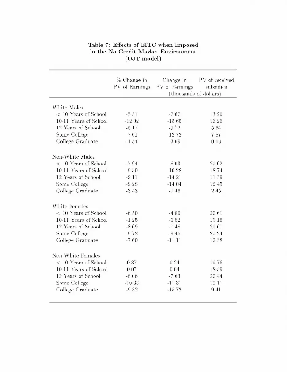
Table 7: E�ects of EITC when Imposedin the No Credit Market Environment

(OJT model)

% Change in Change in PV of receivedPV of Earnings PV of Earnings subsidies

(thousands of dollars)

White Males< 10 Years of School -5.51 -7.67 13.2010-11 Years of School -12.02 -15.65 16.2612 Years of School -5.17 -9.72 5.64Some College -7.01 -12.72 7.87College Graduate -1.54 -3.69 0.63

Non-White Males< 10 Years of School -7.94 -8.03 20.0210-11 Years of School -9.30 -10.28 18.7412 Years of School -9.11 -14.21 11.39Some College -9.28 -14.04 12.45College Graduate -3.43 -7.46 2.45

White Females< 10 Years of School -6.50 -4.80 20.6110-11 Years of School -1.25 -0.82 19.1612 Years of School -8.09 -7.48 20.61Some College -9.72 -9.45 20.24College Graduate -7.60 -11.11 12.58

Non-White Females< 10 Years of School 0.37 0.24 19.7610-11 Years of School 0.07 0.04 18.3912 Years of School -8.06 -7.63 20.44Some College -10.33 -11.31 19.11College Graduate -9.32 -15.72 9.41

Table 8: Decomposition of Changes in Wage Income Due to EITCModel with Perfect Credit Markets

(OJT Simulations Based on 1994 EITC Schedule for Two Children)

PV PV PV(h dH) (H dI) (H dL) Total

White Males< 10 Years of School -5.313 5.260 -8.739 -8.57410-11 Years of School -0.954 0.850 -13.648 -13.63012 Years of School 5.502 -5.852 -8.106 -8.542Some College 2.267 -2.419 -11.799 -11.990College Graduate 3.204 -3.557 -3.861 -4.184

Non-White Males< 10 Years of School -7.519 7.390 -9.447 -9.10210-11 Years of School -2.688 2.417 -10.070 -10.06412 Years of School -0.528 0.439 -13.513 -13.512Some College 0.453 -0.490 -12.931 -12.973College Graduate 3.019 -3.266 -7.785 -8.046

White Females< 10 Years of School -0.483 0.449 -4.684 -4.67610-11 Years of School -0.627 0.565 -1.282 -1.29412 Years of School -3.610 3.453 -8.858 -8.652Some College -1.106 0.984 -9.691 -9.667College Graduate -2.236 2.165 -11.546 -11.464

Non-White Females< 10 Years of School -0.335 0.316 -0.082 -0.08710-11 Years of School -0.679 0.629 -0.479 -0.48912 Years of School -2.716 2.482 -8.352 -8.293Some College -1.087 0.991 -10.695 -10.674College Graduate 0.511 -0.597 -14.044 -14.099

Notes: H=human capital, I=investment, L=leisure, h=1� I � L=hours worked,

dx = change in variable x

Table 9: Annual Compensation (in thousand of dollars) Necessary to MakePeople Indi�erent between Employment and Unemployment

(OJT Simulations Based on 1994 EITC Schedule for Two Children)

With Perfect Credit Markets Without Credit Markets

no EITC with EITC no EITC with EITC

White Males

< 10 Years of School 13.36 13.31 14.59 14.57

10-11 Years of School 9.44 9.19 10.62 10.43

12 Years of School 15.57 15.44 16.08 15.87

Some College 13.54 13.17 14.21 13.76

College Graduate 20.54 20.27 20.66 20.29

Non-White Males

< 10 Years of School 9.41 9.37 11.29 11.28

10-11 Years of School 8.96 8.79 10.47 10.39

12 Years of School 12.02 11.94 12.86 12.80

Some College 11.36 11.09 12.31 12.06

College Graduate 17.49 17.25 17.76 17.41

White Females

< 10 Years of School 5.40 5.39 7.04 7.04

10-11 Years of School 4.84 4.79 6.32 6.29

12 Years of School 6.70 6.69 8.33 8.33

Some College 7.12 7.05 8.69 8.66

College Graduate 12.43 12.38 13.46 13.44

Non-White Females

< 10 Years of School 4.95 4.95 6.52 6.52

10-11 Years of School 4.49 4.47 5.90 5.88

12 Years of School 7.52 7.48 9.22 9.21

Some College 8.82 8.75 10.40 10.37

College Graduate 12.46 12.42 13.10 13.07

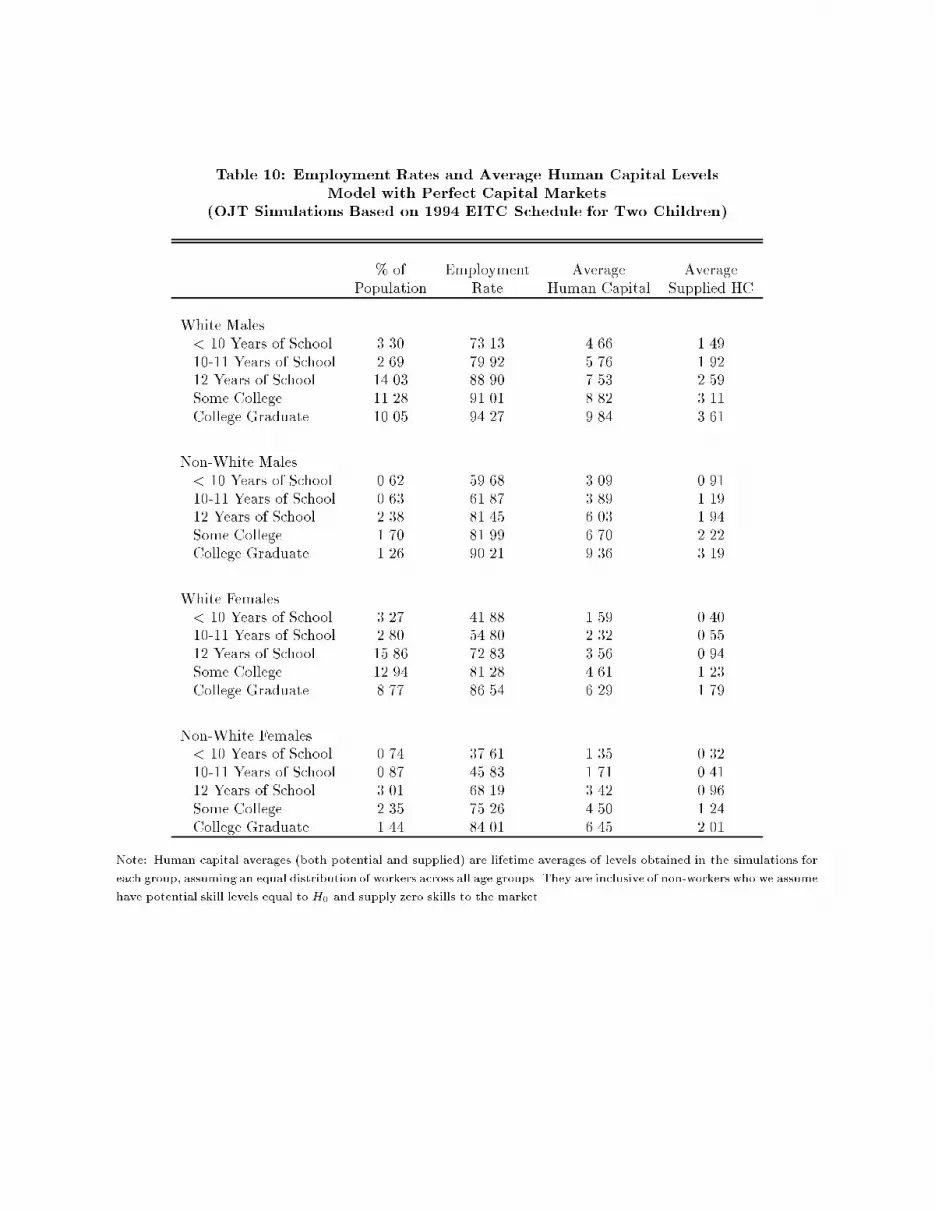
Table 10: Employment Rates and Average Human Capital LevelsModel with Perfect Capital Markets

(OJT Simulations Based on 1994 EITC Schedule for Two Children)

% of Employment Average AveragePopulation Rate Human Capital Supplied HC

White Males< 10 Years of School 3.30 73.13 4.66 1.4910-11 Years of School 2.69 79.92 5.76 1.9212 Years of School 14.03 88.90 7.53 2.59Some College 11.28 91.01 8.82 3.11College Graduate 10.05 94.27 9.84 3.61

Non-White Males< 10 Years of School 0.62 59.68 3.09 0.9110-11 Years of School 0.63 61.87 3.89 1.1912 Years of School 2.38 81.45 6.03 1.94Some College 1.70 81.99 6.70 2.22College Graduate 1.26 90.21 9.36 3.19

White Females< 10 Years of School 3.27 41.88 1.59 0.4010-11 Years of School 2.80 54.80 2.32 0.5512 Years of School 15.86 72.83 3.56 0.94Some College 12.94 81.28 4.61 1.23College Graduate 8.77 86.54 6.29 1.79

Non-White Females< 10 Years of School 0.74 37.61 1.35 0.3210-11 Years of School 0.87 45.83 1.71 0.4112 Years of School 3.01 68.19 3.42 0.96Some College 2.35 75.26 4.50 1.24College Graduate 1.44 84.01 6.45 2.01

Note: Human capital averages (both potential and supplied) are lifetime averages of levels obtained in the simulations for

each group, assuming an equal distribution of workers across all age groups. They are inclusive of non-workers who we assume

have potential skill levels equal to H0 and supply zero skills to the market.

Table 11: E�ects of EITC on Potential Skill LevelsModel with Perfect Capital Markets

(OJT Simulations Based on 1994 EITC Schedule for Two Children)

Di�erence in Change in Average HC Due to Changes in:Average HC Intensive Margin (those whobetween Extensive Margin (entry) would also work under no-EITC)

Workers and (Increase in Employment) Unweighted WeightedNon-Workers 1% 3% 5% 7% (by employment rate)

(1) (2) (3) (4) (5) (6) (7)

White Males< 10 Years of School 0.8685 0.0087 0.0261 0.0434 0.0608 -0.4960 -0.362810-11 Years of School 2.6327 0.0263 0.0790 0.1316 0.1843 -0.0370 -0.029612 Years of School 2.6331 0.0263 0.0790 0.1317 0.1843 0.4765 0.4236Some College 3.9265 0.0393 0.1178 0.1963 0.2749 0.1981 0.1803College Graduate 3.2697 0.0327 0.0981 0.1635 0.2289 0.1693 0.1596

Non-White Males< 10 Years of School 0.4738 0.0047 0.0142 0.0237 0.0332 -0.7338 -0.437910-11 Years of School 1.9565 0.0196 0.0587 0.0978 0.1370 -0.2282 -0.141212 Years of School 1.7827 0.0178 0.0535 0.0891 0.1248 0.0769 0.0627Some College 2.9992 0.0300 0.0900 0.1500 0.2099 0.0611 0.0501College Graduate 3.2945 0.0329 0.0988 0.1647 0.2306 0.2116 0.1908

White Females< 10 Years of School 0.2765 0.0028 0.0083 0.0138 0.0194 -0.0518 -0.021710-11 Years of School 0.9527 0.0095 0.0286 0.0476 0.0667 -0.0977 -0.053512 Years of School 0.2675 0.0027 0.0080 0.0134 0.0187 -0.4471 -0.3256Some College 1.2814 0.0128 0.0384 0.0641 0.0897 -0.1324 -0.1076College Graduate 1.0920 0.0109 0.0328 0.0546 0.0764 -0.2499 -0.2163

Non-White Females< 10 Years of School 0.2847 0.0028 0.0085 0.0142 0.0199 -0.0603 -0.022710-11 Years of School 0.6368 0.0064 0.0191 0.0318 0.0446 -0.1144 -0.052412 Years of School 0.7835 0.0078 0.0235 0.0392 0.0548 -0.3095 -0.2110Some College 1.3186 0.0132 0.0396 0.0659 0.0923 -0.1139 -0.0857College Graduate 1.4334 0.0143 0.0430 0.0717 0.1003 0.1497 0.1258

Aggregate Net E�ects of EITC on Average Human Capital for All Groups(Inclusive of E�ects at Extensive Margin)

AverageHuman Capital (Increase in Employment)(no EITC) 1% 3% 5% 7%

Total e�ects for all groups 5.9246 0.0084 0.0446 0.0809 0.1172Total e�ect assuming no entrye�ects for people withcollege education 5.9246 -0.0034 0.0093 0.0220 0.0348

Total e�ect for people with12 or less years of education 5.9246 -0.0100 0.0028 0.0155 0.0282

Note: Human capital averages are lifetime averages of levels obtained in the simulations for each group, assuming an equal

distribution of workers across all age groups. They are inclusive of non-workers who we assume have potential skill levels

equal to H0.

The values assumed for increase in employment denote percentage points of increase.

Table 12: E�ects of EITC on Skills Supplied to the MarketModel with Perfect Capital Markets

(OJT Simulations Based on 1994 EITC Schedule for Two Children)

Di�erence in Change in Average Suppied HC Due to Changes in:Avg Supplied HC Intensive Margin (those who

between Extensive Margin (entry) would also work under no-EITC)Workers and (Increase in Employment) Unweighted WeightedNon-Workers 1% 3% 5% 7% (by employment rate)

(1) (2) (3) (4) (5) (6) (7)

White Males< 10 Years of School 1.7805 0.0178 0.0534 0.0890 0.1246 -0.2540 -0.185710-11 Years of School 2.2596 0.0226 0.0678 0.1130 0.1582 -0.1458 -0.116512 Years of School 3.0616 0.0306 0.0918 0.1531 0.2143 0.1472 0.1308Some College 3.4519 0.0345 0.1036 0.1726 0.2416 0.0376 0.0342College Graduate 3.8951 0.0390 0.1169 0.1948 0.2727 0.0623 0.0588

Non-White Males< 10 Years of School 1.2039 0.0120 0.0361 0.0602 0.0843 -0.3191 -0.190510-11 Years of School 1.6925 0.0169 0.0508 0.0846 0.1185 -0.2314 -0.143212 Years of School 2.3095 0.0231 0.0693 0.1155 0.1617 -0.0743 -0.0605Some College 2.6552 0.0266 0.0797 0.1328 0.1859 -0.0504 -0.0413College Graduate 3.6022 0.0360 0.1081 0.1801 0.2522 0.0665 0.0600

White Females< 10 Years of School 0.8558 0.0086 0.0257 0.0428 0.0599 -0.0919 -0.038510-11 Years of School 0.8893 0.0089 0.0267 0.0445 0.0622 -0.1225 -0.067112 Years of School 1.0286 0.0103 0.0309 0.0514 0.0720 -0.2631 -0.1916Some College 1.2807 0.0128 0.0384 0.0640 0.0896 -0.2332 -0.1895College Graduate 1.8585 0.0186 0.0558 0.0929 0.1301 -0.2157 -0.1867

Non-White Females< 10 Years of School 0.7903 0.0079 0.0237 0.0395 0.0553 -0.0555 -0.020910-11 Years of School 0.8105 0.0081 0.0243 0.0405 0.0567 -0.0909 -0.041612 Years of School 1.1659 0.0117 0.0350 0.0583 0.0816 -0.2427 -0.1655Some College 1.4533 0.0145 0.0436 0.0727 0.1017 -0.1955 -0.1471College Graduate 2.3678 0.0237 0.0710 0.1184 0.1657 -0.0229 -0.0192

Aggregate Net E�ects of EITC on Average Supplied Human Capital for All Groups(Inclusive of E�ects at Extensive Margin)

AverageSupplied HC (Increase in Employment)(no EITC) 1% 3% 5% 7%

Total e�ects for all groups 1.9029 -0.0467 -0.0036 0.0395 0.0826Total e�ect assuming no entrye�ects for people withcollege education 1.9029 -0.0594 -0.0417 -0.0240 -0.0062

Total e�ect for people with12 or less years of education 1.9029 -0.0246 -0.0069 0.0108 0.0286

Note: Supplied human capital averages are lifetime averages of levels obtained in the simulations for each group, assuming

an equal distribution of workers across all age groups. They are inclusive of non-workers who we assume have potential skill

levels equal to H0 and supply zero skills to the market.

The values assumed for increase in employment denote percentage points of increase.

Table 13: Estimated Life-Cycle Progression Through the EITC ScheduleModel with Perfect Credit Markets

(LBD Simulations Based on 1994 EITC Schedule for Two Children)

Initial Final

EITC Region EITC Region

White Males

< 10 Years of School plateau phase-out

10-11 Years of School plateau beyond

12 Years of School phase-out beyond

Some College phase-out beyond

College Graduate phase-out beyond

Non-White Males

< 10 Years of School plateau1 phase-out

10-11 Years of School plateau1 phase-out

12 Years of School phase-out beyond

Some College phase-out2 beyond

College Graduate phase-out beyond

White Females

< 10 Years of School phase-in plateau

10-11 Years of School plateau1 phase-out

12 Years of School plateau phase-out

Some College plateau1 phase-out2

College Graduate phase-out phase-out

Non-White Females

< 10 Years of School phase-in phase-in

10-11 Years of School plateau1 plateau

12 Years of School phase-in1 plateau2

Some College plateau phase-out

College Graduate phase-out beyond

Notes: 1 Denotes kink between `phase-in' and `plateau' regions.

Notes: 2 Denotes kink between `plateau' and `phase-out' regions.

Table 14: E�ects of EITC when Imposedin the Perfect Credit Market Environment

(LBD model)

% Change in Change in PV of receivedPV of Earnings PV of Earnings subsidies

(thousands of dollars)

White Males< 10 Years of School -12.62 -16.77 15.8110-11 Years of School -13.49 -18.05 15.9012 Years of School -4.91 -9.21 7.53Some College -8.57 -15.82 9.59College Graduate -2.89 -6.46 5.98

Non-White Males< 10 Years of School -13.90 -13.86 19.6310-11 Years of School -18.09 -19.43 19.4012 Years of School -15.98 -23.92 14.47Some College -14.88 -21.79 15.09College Graduate -4.64 -9.71 5.99

White Females< 10 Years of School -4.34 -3.12 20.1810-11 Years of School -12.71 -10.38 20.5912 Years of School -14.20 -13.25 20.60Some College -18.14 -17.88 20.48College Graduate -12.91 -18.21 14.75

Non-White Females< 10 Years of School 1.26 0.70 16.9010-11 Years of School -13.30 -10.91 20.6112 Years of School -15.26 -13.87 20.58Some College -19.85 -20.81 20.35College Graduate -13.87 -22.09 12.68

Table 15: E�ects of EITC when Imposedin the No Credit Market Environment

(LBD model)

% Change in Change in PV of receivedPV of Earnings PV of Earnings subsidies

(thousands of dollars)

White Males< 10 Years of School -15.12 -19.91 16.7010-11 Years of School -15.93 -20.96 16.9112 Years of School -6.20 -11.54 7.01Some College -9.65 -17.53 8.54College Graduate -2.96 -6.51 5.14

Non-White Males< 10 Years of School -15.60 -15.43 20.2110-11 Years of School -19.38 -20.60 20.2612 Years of School -16.58 -24.64 14.56Some College -18.26 -26.40 15.58College Graduate -4.59 -9.48 4.84

White Females< 10 Years of School -4.31 -3.09 20.3010-11 Years of School -13.86 -11.29 20.6112 Years of School -12.64 -11.76 20.61Some College -17.00 -16.70 20.61College Graduate -13.04 -18.30 14.89

Non-White Females< 10 Years of School 1.27 0.70 16.8710-11 Years of School -14.55 -11.93 20.6112 Years of School -15.84 -14.36 20.61Some College -18.83 -19.68 20.60College Graduate -14.92 -23.63 12.65

Table 16: Decomposition of Changes in Wage Income Due to EITCModel with Perfect Credit Markets

(LBD Simulations Based on 1994 EITC Schedule for Two Children)

PV PV(h dH) (H dL) Total

White Males< 10 Years of School -1.754 -15.279 -16.76710-11 Years of School -2.847 -15.604 -18.05512 Years of School -1.803 -7.456 -9.208Some College -3.122 -12.860 -15.821College Graduate -1.929 -4.564 -6.464

Non-White Males< 10 Years of School -0.875 -13.191 -13.86210-11 Years of School -1.526 -18.351 -19.43212 Years of School -2.837 -21.494 -23.918Some College -3.137 -19.088 -21.794College Graduate -2.020 -7.732 -9.708

White Females< 10 Years of School 0.003 -3.123 -3.11710-11 Years of School -0.297 -10.167 -10.37712 Years of School -0.661 -12.691 -13.248Some College -0.836 -17.304 -17.883College Graduate -1.798 -16.627 -18.214

Non-White Females< 10 Years of School 0.035 0.662 0.69710-11 Years of School -0.263 -10.714 -10.90912 Years of School -0.554 -13.455 -13.872Some College -1.059 -20.091 -20.805College Graduate -2.447 -19.953 -22.086

Notes: H=human capital, L=leisure, h=1 � L=hours worked,

dx = change in variable x

Table 17: Annual Compensation (in thousand of dollars) Necessary to MakePeople Indi�erent between Employment and Unemployment

(LBD Simulations Based on 1994 EITC Schedule for Two Children)

With Perfect Credit Markets Without Credit Markets

no EITC with EITC no EITC with EITC

White Males

< 10 Years of School 8.08 7.86 9.07 8.97

10-11 Years of School 7.64 7.36 8.59 8.44

12 Years of School 13.78 13.42 14.32 13.98

Some College 11.70 11.34 12.28 11.90

College Graduate 18.97 17.82 19.47 18.38

Non-White Males

< 10 Years of School 5.65 5.51 6.86 6.81

10-11 Years of School 5.30 5.16 6.36 6.31

12 Years of School 8.62 8.47 9.43 9.32

Some College 8.16 7.96 9.02 8.86

College Graduate 15.04 14.61 15.44 14.98

White Females

< 10 Years of School 5.10 5.08 6.65 6.64

10-11 Years of School 4.01 3.98 5.18 5.18

12 Years of School 5.39 5.36 6.73 6.72

Some College 4.91 4.84 6.06 6.04

College Graduate 9.43 9.30 10.42 10.33

Non-White Females

< 10 Years of School 3.61 3.59 4.77 4.76

10-11 Years of School 4.03 4.02 5.23 5.22

12 Years of School 4.50 4.45 5.68 5.66

Some College 5.05 4.99 6.15 6.14

College Graduate 9.42 9.29 10.13 10.03

Table 18: Employment Rates and Average Human Capital LevelsModel with Perfect Capital Markets

(LBD Simulations Based on 1994 EITC Schedule for Two Children)

% of Employment Average AveragePopulation Rate Human Capital Supplied HC

White Males< 10 Years of School 3.30 73.13 4.45 1.4710-11 Years of School 2.69 79.92 5.42 1.8412 Years of School 14.03 88.90 7.05 2.50Some College 11.28 91.01 7.96 2.88College Graduate 10.05 94.27 9.83 3.73

Non-White Males< 10 Years of School 0.62 59.68 2.94 0.9110-11 Years of School 0.63 61.87 3.47 1.1212 Years of School 2.38 81.45 5.55 1.84Some College 1.70 81.99 5.98 1.99College Graduate 1.26 90.21 8.71 3.06

White Females< 10 Years of School 3.27 41.88 1.54 0.3910-11 Years of School 2.80 54.80 2.39 0.6412 Years of School 15.86 72.83 3.43 0.94Some College 12.94 81.28 4.34 1.18College Graduate 8.77 86.54 5.94 1.74

Non-White Females< 10 Years of School 0.74 37.61 1.27 0.2810-11 Years of School 0.87 45.83 1.81 0.5012 Years of School 3.01 68.19 3.16 0.90Some College 2.35 75.26 4.15 1.20College Graduate 1.44 84.01 6.17 1.95

Note: Human capital averages (both potential and supplied) are lifetime averages of levels obtained in the simulations for

each group, assuming an equal distribution of workers across all age groups. They are inclusive of non-workers who we assume

have potential skill levels equal to H0 and supply zero skills to the market.

Table 19: E�ects of EITC on Potential Skill LevelsModel with Perfect Capital Markets

(LBD Simulations Based on 1994 EITC Schedule for Two Children)

Di�erence in Change in Average HC Due to Changes in:Average HC Intensive Margin (those whobetween Extensive Margin (entry) would also work under no-EITC)

Workers and (Increase in Employment) Unweighted WeightedNon-Workers 1% 3% 5% 7% (by employment rate)

(1) (2) (3) (4) (5) (6) (7)

White Males< 10 Years of School 2.2159 0.0222 0.0665 0.1108 0.1551 0.0222 0.016310-11 Years of School 2.6936 0.0269 0.0808 0.1347 0.1886 -0.1123 -0.089712 Years of School 2.9668 0.0297 0.0890 0.1483 0.2077 -0.0283 -0.0251Some College 3.4262 0.0343 0.1028 0.1713 0.2398 -0.1210 -0.1101College Graduate 5.6936 0.0569 0.1708 0.2847 0.3986 -0.0482 -0.0455

Non-White Males< 10 Years of School 1.7035 0.0170 0.0511 0.0852 0.1192 0.0398 0.023710-11 Years of School 1.7787 0.0178 0.0534 0.0889 0.1245 -0.0449 -0.027812 Years of School 1.9416 0.0194 0.0582 0.0971 0.1359 -0.0726 -0.0591Some College 2.3888 0.0239 0.0717 0.1194 0.1672 -0.1398 -0.1146College Graduate 3.8302 0.0383 0.1149 0.1915 0.2681 -0.0601 -0.0542

White Females< 10 Years of School 0.6441 0.0064 0.0193 0.0322 0.0451 0.0186 0.007810-11 Years of School 0.7197 0.0072 0.0216 0.0360 0.0504 -0.0015 -0.000812 Years of School 0.9035 0.0090 0.0271 0.0452 0.0632 -0.0039 -0.0028Some College 1.3344 0.0133 0.0400 0.0667 0.0934 0.0365 0.0296College Graduate 1.9470 0.0195 0.0584 0.0974 0.1363 -0.0070 -0.0061

Non-White Females< 10 Years of School 0.5198 0.0052 0.0156 0.0260 0.0364 0.0011 0.000410-11 Years of School 0.5485 0.0055 0.0165 0.0274 0.0384 0.0219 0.010012 Years of School 0.9857 0.0099 0.0296 0.0493 0.0690 0.0194 0.0132Some College 1.2346 0.0123 0.0370 0.0617 0.0864 -0.0064 -0.0048College Graduate 1.8863 0.0189 0.0566 0.0943 0.1320 -0.0679 -0.0571

Aggregate Net E�ects of EITC on Average Human Capital for All Groups(Inclusive of E�ects at Extensive Margin)

AverageHuman Capital (Increase in Employment)(no EITC) 1% 3% 5% 7%

Total e�ects for all groups 5.6049 -0.0008 0.0452 0.0912 0.1372Total e�ect assuming no entrye�ects for people withcollege education 5.6049 -0.0153 0.0018 0.0188 0.0359

Total e�ect for people with12 or less years of education 5.6049 0.0020 0.0190 0.0361 0.0531

Note: Human capital averages are lifetime averages of levels obtained in the simulations for each group, assuming an equal

distribution of workers across all age groups. They are inclusive of non-workers who we assume have potential skill levels

equal to H0.

The values assumed for increase in employment denote percentage points of increase.

Table 20: E�ects of EITC on Skills Supplied to the MarketModel with Perfect Capital Markets

(LBD Simulations Based on 1994 EITC Schedule for Two Children)

Di�erence in Change in Average Supplied HC Due to Changes in:Avg Supplied HC Intensive Margin (those who

between Extensive Margin (entry) would also work under no-EITC)Workers and (Increase in Employment) Unweighted WeightedNon-Workers 1% 3% 5% 7% (by employment rate)

(1) (2) (3) (4) (5) (6) (7)

White Males< 10 Years of School 1.8172 0.0182 0.0545 0.0909 0.1272 -0.1925 -0.140810-11 Years of School 2.1586 0.0216 0.0648 0.1079 0.1511 -0.1461 -0.116812 Years of School 2.7897 0.0279 0.0837 0.1395 0.1953 -0.0280 -0.0249Some College 3.0872 0.0309 0.0926 0.1544 0.2161 -0.0752 -0.0684College Graduate 3.9209 0.0392 0.1176 0.1960 0.2745 -0.0341 -0.0321

Non-White Males< 10 Years of School 1.2665 0.0127 0.0380 0.0633 0.0887 -0.2527 -0.150810-11 Years of School 1.3944 0.0139 0.0418 0.0697 0.0976 -0.4081 -0.252512 Years of School 2.0936 0.0209 0.0628 0.1047 0.1465 -0.1679 -0.1368Some College 2.2876 0.0229 0.0686 0.1144 0.1601 -0.1437 -0.1178College Graduate 3.3518 0.0335 0.1006 0.1676 0.2346 -0.0351 -0.0317

White Females< 10 Years of School 0.8558 0.0086 0.0257 0.0428 0.0599 -0.0762 -0.031910-11 Years of School 0.9450 0.0094 0.0283 0.0472 0.0661 -0.2183 -0.119612 Years of School 1.0266 0.0103 0.0308 0.0513 0.0719 -0.2572 -0.1874Some College 1.0745 0.0107 0.0322 0.0537 0.0752 -0.3820 -0.3105College Graduate 1.8136 0.0181 0.0544 0.0907 0.1270 -0.1998 -0.1729

Non-White Females< 10 Years of School 0.7389 0.0074 0.0222 0.0369 0.0517 0.0062 0.002310-11 Years of School 0.9109 0.0091 0.0273 0.0455 0.0638 -0.1762 -0.080712 Years of School 1.0186 0.0102 0.0306 0.0509 0.0713 -0.3025 -0.2063Some College 1.1346 0.0113 0.0340 0.0567 0.0794 -0.4548 -0.3423College Graduate 2.2325 0.0223 0.0670 0.1116 0.1563 -0.0908 -0.0763

Aggregate Net E�ects of EITC on Average Supplied Human Capital for All Groups(Inclusive of E�ects at Extensive Margin)

AverageSupplied HC (Increase in Employment)(no EITC) 1% 3% 5% 7%

Total e�ects for all groups 1.8527 -0.1157 -0.0754 -0.0350 0.0053Total e�ect assuming no entrye�ects for people withcollege education 1.8527 -0.1275 -0.1108 -0.0940 -0.0773

Total e�ect for people with12 or less years of education 1.8527 -0.0497 -0.0330 -0.0162 0.0005

Note: Supplied human capital averages are lifetime averages of levels obtained in the simulations for each group, assuming

an equal distribution of workers across all age groups. They are inclusive of non-workers who we assume have potential skill

levels equal to H0 and supply zero skills to the market.

The values assumed for increase in employment denote percentage points of increase.

Figure 1Earned Income Tax Credit

Earnings

Cre

dit

a b c

sb

Figure 2: Simulated E�ects of EITC on Investment (OJT model)

No EITC

EITC

No EITC (C.C.)

EITC (C.C.)

1 2 3 4 5 6 7 8 9 100

1

2

3

4

5

6x 10

−3

period (5 year age period)

prop

ortio

n of

tim

e in

vest

ing

(I)

Non−White Females − Less than 10th grade

No EITC

EITC

No EITC (C.C.)

EITC (C.C.)

1 2 3 4 5 6 7 8 9 100

0.002

0.004

0.006

0.008

0.01

0.012

period (5 year age period)

prop

ortio

n of

tim

e in

vest

ing

(I)

Non−White Females − 10−11th grade

No EITC

EITC

No EITC (C.C.)

EITC (C.C.)

1 2 3 4 5 6 7 8 9 100

0.002

0.004

0.006

0.008

0.01

0.012

0.014

0.016

0.018

period (5 year age period)

prop

ortio

n of

tim

e in

vest

ing

(I)

White Females − HS graduates

No EITC

EITC

No EITC (C.C.)

EITC (C.C.)

1 2 3 4 5 6 7 8 9 100

0.005

0.01

0.015

0.02

0.025

0.03

period (5 year age period)

prop

ortio

n of

tim

e in

vest

ing

(I)

Non−White Males − HS graduates

Figure 3: Simulated E�ects of EITC on Hours Worked (OJT model)

No EITC

EITC

No EITC (C.C.)

EITC (C.C.)

1 2 3 4 5 6 7 8 9 100.21

0.215

0.22

0.225

0.23

0.235

0.24

0.245

0.25

period (5 year age period)

prop

ortio

n of

tim

e w

orki

ng (

h)

Non−White Females − Less than 10th grade

No EITC

EITC

No EITC (C.C.)

EITC (C.C.)

1 2 3 4 5 6 7 8 9 100.2

0.21

0.22

0.23

0.24

0.25

0.26

0.27

period (5 year age period)

prop

ortio

n of

tim

e w

orki

ng (

h)

Non−White Females − 10−11th grade

No EITC

EITC

No EITC (C.C.)

EITC (C.C.)

1 2 3 4 5 6 7 8 9 100.22

0.23

0.24

0.25

0.26

0.27

0.28

0.29

period (5 year age period)

prop

ortio

n of

tim

e w

orki

ng (

h)

White Females − HS graduates

No EITC

EITC

No EITC (C.C.)

EITC (C.C.)

1 2 3 4 5 6 7 8 9 100.24

0.26

0.28

0.3

0.32

0.34

0.36

period (5 year age period)

prop

ortio

n of

tim

e w

orki

ng (

h)

Non−White Males − HS graduates

Figure 4: Simulated E�ects of EITC on Human Capital (OJT model)

No EITC

EITC

No EITC (C.C.)

EITC (C.C.)

1 2 3 4 5 6 7 8 9 103.2

3.3

3.4

3.5

3.6

3.7

3.8

3.9

period (5 year age period)

hum

an c

apita

l

Non−White Females − Less than 10th grade

No EITC

EITC

No EITC (C.C.)

EITC (C.C.)

1 2 3 4 5 6 7 8 9 102.8

3

3.2

3.4

3.6

3.8

4

4.2

4.4

period (5 year age period)

hum

an c

apita

l

Non−White Females − 10−11th grade

No EITC

EITC

No EITC (C.C.)

EITC (C.C.)

1 2 3 4 5 6 7 8 9 104

4.5

5

period (5 year age period)

hum

an c

apita

l

White Females − HS graduates

No EITC

EITC

No EITC (C.C.)

EITC (C.C.)

1 2 3 4 5 6 7 8 9 105.5

6

6.5

7

7.5

8

8.5

9

period (5 year age period)

hum

an c

apita

l

Non−White Males − HS graduates

Figure 5: Simulated E�ects of EITC on Wage Rates (OJT model)

No EITC

EITC

No EITC (C.C.)

EITC (C.C.)

1 2 3 4 5 6 7 8 9 103.1

3.2

3.3

3.4

3.5

3.6

3.7

3.8

3.9

period (5 year age period)

hour

ly w

age

Non−White Females − Less than 10th grade

No EITC

EITC

No EITC (C.C.)

EITC (C.C.)

1 2 3 4 5 6 7 8 9 102.8

3

3.2

3.4

3.6

3.8

4

4.2

4.4

period (5 year age period)

hour

ly w

age

Non−White Females − 10−11th grade

No EITC

EITC

No EITC (C.C.)

EITC (C.C.)

1 2 3 4 5 6 7 8 9 103.8

4

4.2

4.4

4.6

4.8

5

5.2

5.4

period (5 year age period)

hour

ly w

age

White Females − HS graduates

No EITC

EITC

No EITC (C.C.)

EITC (C.C.)

1 2 3 4 5 6 7 8 9 105

5.5

6

6.5

7

7.5

8

8.5

9

period (5 year age period)

hour

ly w

age

Non−White Males − HS graduates

Figure 6: Simulated E�ects of EITC on Wage Income (OJT model)

No EITC

EITC

No EITC (C.C.)

EITC (C.C.)

1 2 3 4 5 6 7 8 9 107.5

8

8.5

9

9.5

10

period (5 year age period)

thou

sand

of d

olla

rs

Non−White Females − Less than 10th grade

No EITC

EITC

No EITC (C.C.)

EITC (C.C.)

1 2 3 4 5 6 7 8 9 106

7

8

9

10

11

12

13

period (5 year age period)

thou

sand

of d

olla

rs

Non−White Females − 10−11th grade

No EITC

EITC

No EITC (C.C.)

EITC (C.C.)

1 2 3 4 5 6 7 8 9 109

10

11

12

13

14

15

16

period (5 year age period)

thou

sand

of d

olla

rs

White Females − HS graduates

No EITC

EITC

No EITC (C.C.)

EITC (C.C.)

1 2 3 4 5 6 7 8 9 1014

16

18

20

22

24

26

28

30

32

34

period (5 year age period)

thou

sand

of d

olla

rs

Non−White Males − HS graduates

Figure 7: Simulated E�ects of EITC on Hours Worked (LBD model)

No EITC

EITC

No EITC (C.C.)

EITC (C.C.)

1 2 3 4 5 6 7 8 9 100.2

0.205

0.21

0.215

0.22

0.225

period (5 year age period)

prop

ortio

n of

tim

e w

orki

ng (

h)

Non−White Females − Less than 10th grade

No EITC

EITC

No EITC (C.C.)

EITC (C.C.)

1 2 3 4 5 6 7 8 9 100.2

0.22

0.24

0.26

0.28

0.3

period (5 year age period)

prop

ortio

n of

tim

e w

orki

ng (

h)

Non−White Females − 10−11th grade

No EITC

EITC

No EITC (C.C.)

EITC (C.C.)

1 2 3 4 5 6 7 8 9 100.2

0.21

0.22

0.23

0.24

0.25

0.26

0.27

0.28

0.29

period (5 year age period)

prop

ortio

n of

tim

e w

orki

ng (

h)

White Females − HS graduates

No EITC

EITC

No EITC (C.C.)

EITC (C.C.)

1 2 3 4 5 6 7 8 9 100.22

0.24

0.26

0.28

0.3

0.32

0.34

0.36

0.38

period (5 year age period)

prop

ortio

n of

tim

e w

orki

ng (

h)

Non−White Males − HS graduates

Figure 8: Simulated E�ects of EITC on Human Capital (LBD model)

No EITC

EITC

No EITC (C.C.)

EITC (C.C.)

1 2 3 4 5 6 7 8 9 102.8

2.9

3

3.1

3.2

3.3

3.4

3.5

3.6

period (5 year age period)

hum

an c

apita

l

Non−White Females − Less than 10th grade

No EITC

EITC

No EITC (C.C.)

EITC (C.C.)

1 2 3 4 5 6 7 8 9 103.4

3.5

3.6

3.7

3.8

3.9

4

4.1

4.2

4.3

period (5 year age period)

hum

an c

apita

l

Non−White Females − 10−11th grade

No EITC

EITC

No EITC (C.C.)

EITC (C.C.)

1 2 3 4 5 6 7 8 9 103.8

4

4.2

4.4

4.6

4.8

5

5.2

period (5 year age period)

hum

an c

apita

l

White Females − HS graduates

No EITC

EITC

No EITC (C.C.)

EITC (C.C.)

1 2 3 4 5 6 7 8 9 104.5

5

5.5

6

6.5

7

7.5

8

period (5 year age period)

hum

an c

apita

l

Non−White Males − HS graduates

Figure 9: Changes in Hourly Wages due to Increases in Hours Worked(LBD model)

Working 100 more hours per year

Working 1 more hour per day

0 1 2 3 4 5 6 7

x 104

−0.03

−0.02

−0.01

0

0.01

0.02

0.03

0.04

0.05

0.06

0.07

accumulated hours worked

dolla

r am

ount

of c

hang

e in

hou

rly w

age

Non−White Females − Less than 10th grade

Working 100 more hours per year

Working 1 more hour per day

0 1 2 3 4 5 6 7 8

x 104

−0.06

−0.04

−0.02

0

0.02

0.04

0.06

0.08

accumulated hours worked

dolla

r am

ount

of c

hang

e in

hou

rly w

age

Non−White Females − 10−11th grade

Working 100 more hours per year

Working 1 more hour per day

0 1 2 3 4 5 6 7 8

x 104

−0.04

−0.02

0

0.02

0.04

0.06

0.08

0.1

accumulated hours worked

dolla

r am

ount

of c

hang

e in

hou

rly w

age

White Females − HS graduates

Working 100 more hours per year

Working 1 more hour per day

0 1 2 3 4 5 6 7 8 9 10

x 104

−0.1

−0.05

0

0.05

0.1

0.15

0.2

accumulated hours worked

dolla

r am

ount

of c

hang

e in

hou

rly w

age

Non−White Males − HS graduates

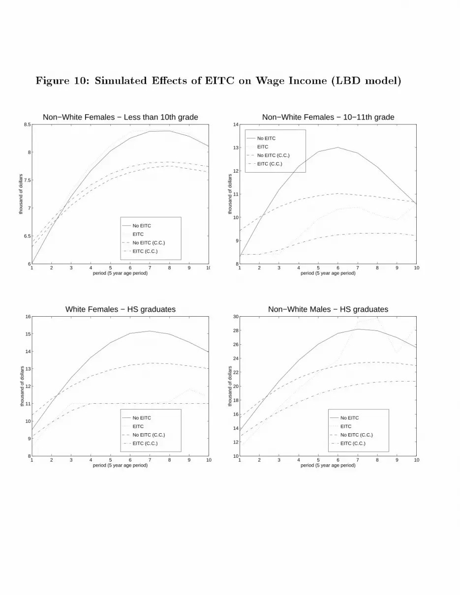
Figure 10: Simulated E�ects of EITC on Wage Income (LBD model)

No EITC

EITC

No EITC (C.C.)

EITC (C.C.)

1 2 3 4 5 6 7 8 9 106

6.5

7

7.5

8

8.5

period (5 year age period)

thou

sand

of d

olla

rs

Non−White Females − Less than 10th grade

No EITC

EITC

No EITC (C.C.)

EITC (C.C.)

1 2 3 4 5 6 7 8 9 108

9

10

11

12

13

14

period (5 year age period)

thou

sand

of d

olla

rs

Non−White Females − 10−11th grade

No EITC

EITC

No EITC (C.C.)

EITC (C.C.)

1 2 3 4 5 6 7 8 9 108

9

10

11

12

13

14

15

16

period (5 year age period)

thou

sand

of d

olla

rs

White Females − HS graduates

No EITC

EITC

No EITC (C.C.)

EITC (C.C.)

1 2 3 4 5 6 7 8 9 1010

12

14

16

18

20

22

24

26

28

30

period (5 year age period)

thou

sand

of d

olla

rs

Non−White Males − HS graduates

Appendix A

Table A-1: De�nition of EITC Regions for CPS Calculations

Region Income Range

I (phase-in) W < 0:95 aII (�rst kink) 0:95 a �W < 1:05 aIII (plateau) 1:05 a �W < 0:95 bIV (second kink) 0:95 b �W < 1:05 bV (phase-out) 1:05 b �W < 0:95 cVI (third kink) 0:95 c �W < 1:05 cVII (no credit) 1:05 c �W

49

Appendix B

Nonconcavity of the Reward Function in the Ben Porath model

in the Presence of an EITC Program

For simplicity, set R = 1, r = 0, H0 = 1. Then consider V (I) for a program where there

is either a phase-out range or a no program range. For I > k, we assume that a person is in

the phase-out range (branch 3). For I � k, we assume that a person is in the no program

range (no tax or subsidy). Using � as the phase-out tax rate, we may write V (I) for two

values of I1 and I2, which in the second period place the individual in the no-EITC zone.

V (I1) = (1 + �)(1� I1)1(I1 > k) + (1� I1)1(I1 � k) + F (I1)

V (I2) = (1 + �)(1� I2)1(I2 > k) + (1� I2)1(I2 � k) + F (I2)

We can always �nd such values of I1 and I2. (This is trivial if the agent starts in the no

program range.) Provided investment is su�ciently productive, we can move the agent from

the phase-out range to the no program range. This requires that we �nd values of I1 such

that (1�I1) < c; F (I1)+1 > c so 1� c < I1; F (I1) > c�1. Assuming F is monotonically

increasing Maxf1 � c; F�1(c� 1)g < I1. Then letting I = �I1 + (1� �)I2; 0 � � � 1;

V (I) = (1 + �)(1 � I)1(I > k) + (1� I)1(I � k) + F (I)

= �(1� I)1(I > k) + (1� �I) + F (I):

Next, we obtain

�V (I1) + (1� �)V (I2)

= ��(1� I1)1(I1 > k) + �(1� I1) + �F (I1)

+(1� �)�(1� I2)1(I2 > k) + (1� �)(1� I2) + (1� �)F (I2)

= (1� �I) + �(�(1� I1)1(I1 > k)) + �((1 � �)(1� I2)1(I2 > k))

+�F (I1) + (1� �)F (I2):

V (I) is concave if

V (I) � �V (I1) + (1� �)V (I2),

or

�(1� I)1(I > k) + F (I) �

� [�(1� I1)1(I1 > k)) + ((1� �)(1� I2)1(I2 > k)] + �F (I1) + (1� �)F (I2).

Clearly, F (I)��F (I1)�(1��)F (I2) � 0 by concavity in F (I). However, it is not necessarily

true that for � > 0

(1� I)1(I > k) � [�(1� I1)1(I1 > k) + (1� �)(1� I2)1(I2 > k)].

50

Provided I > 0; it is possible that I < k, but either I1 or I2 > k. Then our concavity

condition may or may not be true. Thus for certain ranges of values we obtain concavity of

the reward function. However, the result is delicate. If investment is su�ciently productive,

the contribution of F (I) � (�)F (I1) � (1 � �)F (I2) may o�set the non-concavity arising

from the jump in the indicator functions. Non-concavity is not generic for all values of the

parameters but may arise for some values.

51

Appendix C

Solution Algorithm for Individual Optimization Problem

Problems with discontinuity and a non-convex budget set require non-standard solution

methods be employed in solving the individual's optimization problem. This, in part, is

responsible for our reduction of the life cycle problem to ten periods. Because gradient

methods cannot be used, we use the direct search complex algorithm DBCPOL in Fortran

77 to simultaneously solve for all consumption, leisure, and investment (for the OJT model)

values when maximizing lifetime utility subject to the appropriate human and physical

capital accumulation constraints. In the OJT model, this amounts to guessing a path for

investment and leisure. Calculating the optimal consumption path given this investment

and leisure path is trivial. Then, total lifetime utility is found. These steps are iterated

using the DBCPOL algorithm until the maximizing consumption, leisure, and investment

pro�les are found. We use multiple starting values for each pro�le to determine whether the

optimization procedure produces global optima. Reasonable starting values for investment

and leisure generally yielded a global optimum. In particular, we use the optimal paths

for leisure and investment when the EITC is not imposed as initial guesses, and we always

�nd that this leads to a global optimum. A similar procedure is used for the LBD model,

dropping investment I.

52

Appendix D

Parameter Estimates

This appendix reports the parameter estimates and goodness of �t for the models used

in the paper. Tables D-1 and D-2 report the parameter estimates for the OJT and LBD

models, respectively. The weighted sum of squared errors are reported in Tables D-3 and D-

4, along with a decomposition of those errors into the contribution due errors in predicting

hours and wages. Figures D-1 and D-2 show the estimated and mean wage pro�les for the

workers we examine in the paper. The large uctuations in mean wages can be attributed

to the sometimes small sample sizes for some of the workers we examine, particularly those

with less than a high school education. Figures D-3 and D-4 report estimated and mean

hours worked pro�les.

53

Table D-1: Parameter Values for the OJT Model

� B � H0

White Males

< 10 Years of School 0.0792 -9.7102 1.7373 0.8734 5.0103

10-11 Years of School 0.8387 -4.1989 1.2618 0.3239 4.5328

12 Years of School 0.3532 -5.5217 1.5719 0.6899 6.3149

Some College 0.7019 -4.2462 1.6743 0.4244 5.9627

College Graduate 0.2694 -5.6716 1.5668 0.5101 7.3358

Non-White Males

< 10 Years of School 0.1238 -9.6809 1.8485 0.8820 3.9738

10-11 Years of School 0.4491 -6.2600 1.3667 0.4606 4.0993

12 Years of School 0.5817 -4.8789 1.5313 0.6884 5.6933

Some College 0.7169 -4.6215 1.3160 0.3034 5.2365

College Graduate 0.4572 -5.2305 1.5881 0.4767 7.2972

White Females

< 10 Years of School 0.8901 -5.3879 0.8558 0.6015 3.4585

10-11 Years of School 0.8971 -6.4344 0.7270 0.3122 3.1871

12 Years of School 0.8947 -5.0882 1.8262 0.8473 4.1736

Some College 0.8986 -5.4280 0.8636 0.3134 4.2562

College Graduate 0.3274 -7.4619 1.6189 0.7213 5.9213

Non-White Females

< 10 Years of School 0.7751 -6.4974 0.9285 0.6098 3.2512

10-11 Years of School 0.8907 -6.0751 0.9656 0.5064 2.9811

12 Years of School 0.5194 -6.3269 1.3129 0.6186 3.9263

Some College 0.5044 -6.7793 0.9770 0.3740 4.5435

College Graduate 0.7523 -4.4080 1.4460 0.6894 6.3922

Table D-2: Parameter Values for the LBD Model

� H0 �0 �1

White Males

< 10 Years of School 1.3755 -2.7587 3.8919 3.4658 -0.9355

10-11 Years of School 1.6521 -2.5783 3.9816 3.6629 -0.8089

12 Years of School 0.6226 -4.2401 4.9390 4.1659 -1.0071

Some College 1.1328 -3.1976 5.2034 3.6853 -0.6087

College Graduate 0.2074 -6.5865 4.6867 6.2757 -1.1821

Non-White Males

< 10 Years of School 1.7891 -2.4149 3.2587 2.7846 -0.7947

10-11 Years of School 2.6426 -1.5038 3.7872 2.7636 -0.7027

12 Years of School 1.6837 -2.2904 4.8043 2.8065 -0.6748

Some College 1.8593 -2.3070 4.7592 3.1820 -0.6676

College Graduate 0.6907 -4.3959 5.7665 4.4557 -0.8647

White Females

< 10 Years of School 0.9555 -5.1475 3.0491 1.2586 -0.4397

10-11 Years of School 3.0723 -1.3047 3.6451 1.2862 -0.3928

12 Years of School 1.9320 -2.5976 3.8051 1.5468 -0.4592

Some College 2.9105 -1.5383 4.0477 2.5122 -0.8191

College Graduate 1.1191 -3.9764 4.9137 3.2518 -0.9414

Non-White Females

< 10 Years of School 1.5521 -4.8080 2.8516 1.0161 -0.3479

10-11 Years of School 2.8638 -1.1183 3.4269 1.0245 -0.3375

12 Years of School 2.8248 -1.3371 3.6644 1.7231 -0.5218

Some College 3.0720 -1.2175 4.2671 2.1769 -0.6440

College Graduate 1.6362 -2.5354 5.3896 2.8619 -0.7268

Table D-3: Goodness of Fit (OJT Model)Weighted Sum of Squared Di�erences

Wages Hours Total

White Males

< 10 Years of School 57.92 179.99 237.91

10-11 Years of School 219.87 487.90 707.76

12 Years of School 763.13 819.53 1582.66

Some College 345.74 1347.42 1693.15

College Graduate 449.35 413.50 862.86

Non-White Males

< 10 Years of School 13.02 41.55 54.57

10-11 Years of School 39.11 119.97 159.08

12 Years of School 46.51 90.70 137.21

Some College 68.61 149.64 218.26

College Graduate 26.63 35.35 61.99

White Females

< 10 Years of School 16.34 74.86 91.20

10-11 Years of School 63.97 201.01 264.98

12 Years of School 150.16 134.43 284.59

Some College 222.94 415.20 638.15

College Graduate 77.07 137.92 214.99

Non-White Females

< 10 Years of School 8.92 24.92 33.84

10-11 Years of School 46.11 93.95 140.06

12 Years of School 49.00 96.13 145.13

Some College 20.80 101.91 122.71

College Graduate 12.48 14.33 26.80

Table D-4: Goodness of Fit (LBD Model)Weighted Sum of Squared Di�erences

Wages Hours Total

White Males

< 10 Years of School 13.09 53.84 66.93

10-11 Years of School 75.70 280.53 356.23

12 Years of School 85.02 418.02 503.04

Some College 136.13 1114.35 1250.48

College Graduate 19.88 294.29 314.17

Non-White Males

< 10 Years of School 8.27 20.92 29.19

10-11 Years of School 16.87 50.53 67.41

12 Years of School 13.59 25.99 39.58

Some College 33.45 101.25 134.71

College Graduate 16.33 28.49 44.82

White Females

< 10 Years of School 18.04 78.06 96.10

10-11 Years of School 118.15 178.90 297.05

12 Years of School 52.91 91.14 144.05

Some College 86.29 209.71 296.00

College Graduate 31.98 120.93 152.91

Non-White Females

< 10 Years of School 12.13 36.98 49.11

10-11 Years of School 64.02 114.98 179.00

12 Years of School 19.66 19.93 39.59

Some College 12.74 44.29 57.03

College Graduate 4.85 6.25 11.10

Figure D-1: Actual vs. Simulated Wage Earnings Paths (OJT model)

Simulated

Actual

1 2 3 4 5 6 7 8 9 103

3.2

3.4

3.6

3.8

4

4.2Non−White Females − Less than 10th grade

period (5 year age period)

thou

sand

of d

olla

rs

Simulated

Actual

1 2 3 4 5 6 7 8 9 102.6

2.8

3

3.2

3.4

3.6

3.8

4

4.2

4.4Non−White Females − 10−11th grade

period (5 year age period)

thou

sand

of d

olla

rs

Simulated

Actual

1 2 3 4 5 6 7 8 9 103.6

3.8

4

4.2

4.4

4.6

4.8

5

5.2

5.4White Females − HS graduates

period (5 year age period)

thou

sand

of d

olla

rs

Simulated

Actual

1 2 3 4 5 6 7 8 9 104.5

5

5.5

6

6.5

7

7.5

8

8.5

9Non−White Males − HS graduates

period (5 year age period)

thou

sand

of d

olla

rs

Figure D-2: Actual vs. Simulated Wage Earning Paths (LBD model)

Simulated

Actual

1 2 3 4 5 6 7 8 9 102.8

3

3.2

3.4

3.6

3.8

4

4.2Non−White Females − Less than 10th grade

period (5 year age period)

thou

sand

of d

olla

rs

Simulated

Actual

1 2 3 4 5 6 7 8 9 102.6

2.8

3

3.2

3.4

3.6

3.8

4

4.2Non−White Females − 10−11th grade

period (5 year age period)

thou

sand

of d

olla

rs

Simulated

Actual

1 2 3 4 5 6 7 8 9 103.6

3.8

4

4.2

4.4

4.6

4.8

5

5.2White Females − HS graduates

period (5 year age period)

thou

sand

of d

olla

rs

Simulated

Actual

1 2 3 4 5 6 7 8 9 104.5

5

5.5

6

6.5

7

7.5

8

8.5Non−White Males − HS graduates

period (5 year age period)

thou

sand

of d

olla

rs

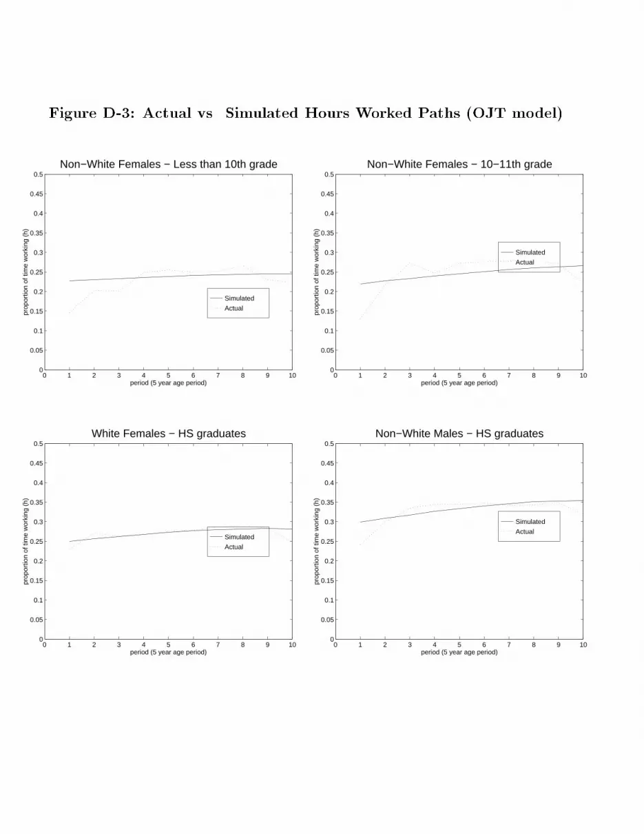
Figure D-3: Actual vs. Simulated Hours Worked Paths (OJT model)

Simulated

Actual

0 1 2 3 4 5 6 7 8 9 100

0.05

0.1

0.15

0.2

0.25

0.3

0.35

0.4

0.45

0.5Non−White Females − Less than 10th grade

period (5 year age period)

prop

ortio

n of

tim

e w

orki

ng (

h)

Simulated

Actual

0 1 2 3 4 5 6 7 8 9 100

0.05

0.1

0.15

0.2

0.25

0.3

0.35

0.4

0.45

0.5Non−White Females − 10−11th grade

period (5 year age period)

prop

ortio

n of

tim

e w

orki

ng (

h)

Simulated

Actual

0 1 2 3 4 5 6 7 8 9 100

0.05

0.1

0.15

0.2

0.25

0.3

0.35

0.4

0.45

0.5White Females − HS graduates

period (5 year age period)

prop

ortio

n of

tim

e w

orki

ng (

h)

Simulated

Actual

0 1 2 3 4 5 6 7 8 9 100

0.05

0.1

0.15

0.2

0.25

0.3

0.35

0.4

0.45

0.5Non−White Males − HS graduates

period (5 year age period)

prop

ortio

n of

tim

e w

orki

ng (

h)

Figure D-4: Actual vs. Simulated Hours Worked Paths (LBD model)

Simulated

Actual

0 1 2 3 4 5 6 7 8 9 100

0.05

0.1

0.15

0.2

0.25

0.3

0.35

0.4

0.45

0.5Non−White Females − Less than 10th grade

period (5 year age period)

prop

ortio

n of

tim

e w

orki

ng (

h)

Simulated

Actual

0 1 2 3 4 5 6 7 8 9 100

0.05

0.1

0.15

0.2

0.25

0.3

0.35

0.4

0.45

0.5Non−White Females − 10−11th grade

period (5 year age period)

prop

ortio

n of

tim

e w

orki

ng (

h)

Simulated

Actual

0 1 2 3 4 5 6 7 8 9 100

0.05

0.1

0.15

0.2

0.25

0.3

0.35

0.4

0.45

0.5White Females − HS graduates

period (5 year age period)

prop

ortio

n of

tim

e w

orki

ng (

h)

Simulated

Actual

0 1 2 3 4 5 6 7 8 9 100

0.05

0.1

0.15

0.2

0.25

0.3

0.35

0.4

0.45

0.5Non−White Males − HS graduates

period (5 year age period)

prop

ortio

n of

tim

e w

orki

ng (

h)