volume mls ray casting
TRANSCRIPT

Volume MLS Ray Casting
(Article begins on next page)
Citation Ledergerber, Christian, Gael Guennebaud, Miriah Meyer, MoritzBacher, and Hanspeter Pfister. 2008. Volume MLS ray casting.IEEE Transactions on Visualization and Computer Graphics 14(6):1372-1379.
Published Version doi:10.1109/TVCG.2008.186
Accessed May 18, 2011 8:29:05 AM EDT
Citable Link http://nrs.harvard.edu/urn-3:HUL.InstRepos:4100249
Terms of Use This article was downloaded from Harvard University's DASHrepository, and is made available under the terms and conditionsapplicable to Open Access Policy Articles, as set forth athttp://nrs.harvard.edu/urn-3:HUL.InstRepos:dash.current.terms-of-use#OAP

Volume MLS Ray Casting
Christian Ledergerber, Gael Guennebaud, Miriah Meyer,
Moritz Bacher and Hanspeter Pfister, Senior Member, IEEE
Abstract— The method of Moving Least Squares (MLS) is a popular framework for reconstructing continuous functions from scattereddata due to its rich mathematical properties and well-understood theoretical foundations. This paper applies MLS to volume rendering,providing a unified mathematical framework for ray casting of scalar data stored over regular as well as irregular grids. We use theMLS reconstruction to render smooth isosurfaces and to compute accurate derivatives for high-quality shading effects. We alsopresent a novel, adaptive preintegration scheme to improve the efficiency of the ray casting algorithm by reducing the overall numberof function evaluations, and an efficient implementation of our framework exploiting modern graphics hardware. The resulting systemenables high-quality volume integration and shaded isosurface rendering for regular and irregular volume data.
Index Terms—Volume Visualization, Unstructured Grids, Moving Least Squares Reconstruction, Adaptive Integration
1 INTRODUCTION
Volume visualization has become an integral component of the sci-entific discovery process and the simulation pipeline. Data comingfrom scanning devices such as MRI or ultrasound machines, as well asresults from simulations in fields like computational fluid dynamics,geophysics, and biomedical computing, are often represented volu-metrically. These volumes, however, can be defined over regular orirregular grids, giving rise to several distinct classes of rendering algo-rithms and a plethora of implementations.
In this paper we propose a unified framework for generatinghigh-quality visualizations of arbitrary volumetric datasets using themethod of Moving Least Squares (MLS). MLS is a popular scheme forreconstructing continuous functions from scattered data due to its wellunderstood mathematical foundations. Furthermore, the MLS frame-work contains several distinct components that provide a high levelof control over the function reconstruction, and allows for a tunableamount of data smoothing as well as interpolation.
Using MLS, we reconstruct continuous functions from data storedon regular as well as irregular grids. We introduce volume MLS raycasting to generate high-quality images with volume integration andisosurfaces, such as that shown in Figure 1.
The volume MLS framework enables computing analytic deriva-tives for high-quality isosurface shading with specularities. To de-crease the over-all number of MLS function evaluations we propose anovel adaptive preintegration technique.
The main contributions of this work are: a unified MLS frameworkfor reconstructing continuous functions and their derivatives from bothregular grids and unstructured volume data; a novel adaptive preinte-gration scheme for ray casting continuous functions with transfer func-tions that include isosurfaces; and a system that combines high-qualityisosurface rendering and volume integration. We provide details on thetheoretical foundations of the MLS framework, along with an explo-ration of the various tunable parameters. We also present an imple-mentation of volume MLS ray casting on modern graphics processorunits (GPUs), provide details of our system implementation, and showresults on several regular and irregular volume data sets.
• C. Ledergerber, M. Meyer, M. Bacher, and H. Pfister are with the IIC at
Harvard University, E-mail: firstname [email protected]
• G. Guennebaud is with CNR of Pisa, E-mail: [email protected]
Manuscript received 31 March 2008; accepted 1 August 2008; posted online
19 October 2008; mailed on 13 October 2008.
For information on obtaining reprints of this article, please send
e-mailto:[email protected].
2 PREVIOUS WORK
Direct Volume Rendering: The generation of high-quality im-ages of volume data relies on methods that accurately solve the vol-ume rendering integral [28], which models a volume as a medium thatcan emit, transmit, and absorb light. The standard method for solv-ing this integral is ray casting, and was proposed by Levoy [21] forregular grids, and by Garrity [14] for irregular grids, specifically tetra-hedral meshes. Splatting, an alternative to ray casting, was proposedby Westover [49] for regular grids, and has been extended to irregulargrids [25, 51]. In either case, a continuous function must be recon-structed from the discrete volume data.
While there are well-established mathematical frameworks for re-construction of continuous functions from regular volume data [10, 18,27, 9], irregular volumes are more challenging as there is no impliedspatial structure to the data points. Ray casting of tetrahedral meshesallows a direct interpolation of the data at ray-triangle intersections us-ing homogeneous coordinates [14]. For curvilinear grids, interpolationis more complicated [45] and is typically performed at the intersectionpoints with cell faces [6] or in computational space [13]. Another pop-ular algorithm for rendering tetrahedral meshes is the cell projectionmethod [42], in which tetrahedral cells are projected in back to frontorder onto the image plane [5, 11]. However, a correct depth-orderingof cells does not always exist, and great care must be taken to avoidvisual artifacts [50]. Finally, another class of algorithms uses a sweep-plane through the volume followed by rendering of 2D cells [15, 43].
In the case where no explicit structure of the data is given, scattereddata reconstruction schemes are applied. Arguably the most promi-nent method among these are radial basis functions (RBFs) that wereintroduced to volume rendering by Jang et al.[17]. While RBFs can beevaluated and rendered efficiently [31], the method requires a costlyinitial solution to a global system of equations, the size of which istied to the number of data points. Other methods proposed in the con-text of volume visualization are inverse distance weighting [35], whichis a special case of MLS [41], and discrete Sibson interpolation [36].This latter method inherently relies on resampling the data onto a reg-ular grid. In contrast to these approaches, volume MLS ray castingprovides a unifying mathematical framework for the reconstruction ofarbitrarily sampled volume data that allows the user to control the re-construction and data smoothing in a principled manner.
MLS Function Reconstruction: MLS was introduced almosthalf a century ago by Shepard [41], and more recently shown byLevin as a powerful surface approximation technique [20]. This tech-nique has been embraced by the computer graphics community forreconstructing point set surfaces [3, 4], where a number of extensionshave been proposed, such as reconstructing surfaces with sharp fea-tures [12, 23] and using anisotropic support regions [1]. Unlike RBFs,MLS does not require a solution to a global system of equations.

Volume Integration: During ray casting, a transfer function (TF),which maps scalar values and (optionally) gradients to colors andopacities, is applied to the volume function. These color and opac-ity properties of the volume are integrated along rays to obtain thefinal pixel colors. The TF must be smooth in order to compute the nu-merical integral efficiently and accurately as no general, closed-formsolutions are available. For the case of a smooth TF, well-known adap-tive numerical schemes can be employed [32], and theory from MonteCarlo integration can guide their design [7]. Also, interval arithmetichas been proposed to make the above approaches robust [33].
In practice, however, smooth TFs limit the range of achievable ren-dering effects, e.g., isosurface rendering via thin spikes in the TF that,in theory, require an infinite sampling density. To circumvent thisproblem Roettger et al. [39] introduce preintegration, which avoidsvisual artifacts by precomputing the volume rendering integral forray segments, assuming that the underlying scalar function is lin-ear. Recent efforts focus on accelerating the precomputation [8, 37],faster approximation algorithms [24], multidimensional transfer func-tions [30], and preintegrated lighting [24, 29].
In this paper we propose an adaptive integration scheme based onpreintegration. This scheme is similar in spirit to other numerical inte-gration schemes, such as adaptive Simpson [32] and the second deriva-tive refinement scheme of Roettger et al. [38].
3 VOLUME MLS
In order to generate high-quality images, a ray caster must evaluate acontinuous representation, and the associated derivatives, of volumet-ric data. For volume data defined over a grid, two approaches can betaken: first, the connectivity of the grid can be used to define a recon-struction scheme over the locally connected data points; or second,the data points can be used independently of their grid connectionsin a scattered data reconstruction scheme. The first approach workswell for regular grids, where higher order polynomials are often em-ployed to reconstruct functions of arbitrary continuity. For irregulargrids, however, reconstructions are challenging for anything other thenpiecewise linear interpolation. Thus, we advocate a unified reconstruc-tion framework that takes the latter approach, allowing for continuousand differentiable representations of regular and irregular grids.
Scattered data reconstruction takes a set of n data points, pi =(xi, fi), defined over a volume V , and computes an approximation(or interpolation) to the data points f (x) : V → R. One such well-studied, meshless scheme is MLS, where f (x) is obtained by approxi-mating the local neighborhood of x in a weighted least squares (WLS)sense. The MLS method has a high degree of flexibility, making itparticularly appealing for the reconstruction of volumetric data, whileavoiding the artifacts often incurred by reconstruction schemes that areconstrained to arbitrarily poor connectivities (i.e., interpolation overpoorly shaped mesh elements). This flexibility provides the capacityfor (controllably) handling noise due to measurement errors in scanneddata or numerical errors in simulated data. Furthermore, the MLS ap-proximation is a continuous reconstruction with well-defined, smoothderivatives which allows for high-quality shading effects.
In this section, we first describe the MLS framework and mathe-matical foundations in the context of reconstructing continuous func-tions from scattered data. We then discuss and explore the variouscomponents of the MLS method as they relate to reconstructing datastored over regular and irregular grids specifically for generating high-quality visualizations by ray casting. Our notation is as follows: boldface lower-case variables denote column vectors, such as x = [x y z]T ,while bold face upper-case variables denote matrices, such as the iden-tity matrix I. We note that the MLS discussion and mathematical def-inition holds for arbitrary dimensions, even though we restrict our ex-amples and results to R
3.
3.1 The MLS Framework
The main idea behind the MLS reconstruction method is depicted fora 1D signal in Figure 2. Shown in red, a continuous approximationf (x) is reconstructed from a set of n data points (xi, fi) by computing
Fig. 1. The continuous temperature function of a simulated heptaneplume rendered with volume MLS ray casting.
Fig. 2. MLS reconstruction of a given set of scattered data points (xi, fi)in 1D. The local WLS approximation gx for the point x is shown in blue.Its computation and evaluation at every point of the domain yields thecomplete MLS reconstruction shown in red.
and evaluating a local approximation gx at x (shown in blue):
f (x) = gx(x). (1)
The local approximation gx is obtained by the following WLS mini-mization problem:
gx = argming
∑i
wi(x)|g(xi)− fi|2, (2)
where wi(x) is the weight of the sample pi for the current evaluationpoint x. These weights typically decrease with distance from x (seeSection 3.1.2). Assuming gx can be represented as a linear combina-tion of k basis functions b(x) = [b1(x), . . . ,bk(x)]T with coefficients
cx = [c1, . . . ,ck]T , Equation 2 can be rewritten in the following matrix
form:cx = min
c∈Rk‖(
√
W(x)Bc− f)‖2, (3)
where W(x) = diag(w1(x), . . . ,wn(x)) ∈ Rn×n and Bi j = bi(x j),B ∈
Rn×k. It is well-known from linear algebra that the above least squares
problem can be solved using the normal equation. Substituting the so-lution for cx into f (x) = b(x)T cx yields the following explicit formu-lation of the MLS approximating function:
f (x) = b(x)T (BT W(x)B)−1BT W(x)f . (4)
This function is smooth, assuming the weights wi(x) are smooth [19],and can be computed as long as the weighted covariance matrixBT W(x)B is invertible, which is the case if rank(W(x)B) ≥ k — this
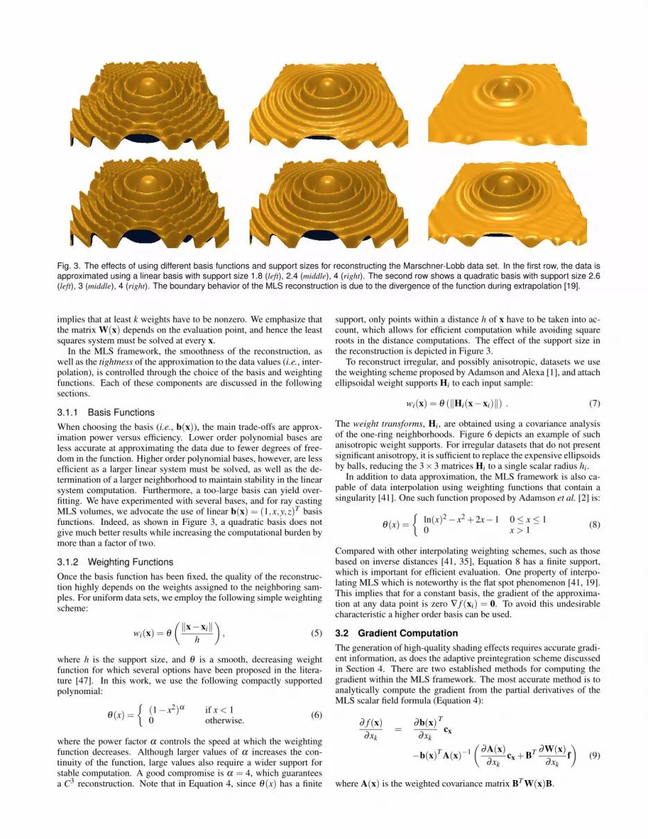
Fig. 3. The effects of using different basis functions and support sizes for reconstructing the Marschner-Lobb data set. In the first row, the data isapproximated using a linear basis with support size 1.8 (left), 2.4 (middle), 4 (right). The second row shows a quadratic basis with support size 2.6(left), 3 (middle), 4 (right). The boundary behavior of the MLS reconstruction is due to the divergence of the function during extrapolation [19].
implies that at least k weights have to be nonzero. We emphasize thatthe matrix W(x) depends on the evaluation point, and hence the leastsquares system must be solved at every x.
In the MLS framework, the smoothness of the reconstruction, aswell as the tightness of the approximation to the data values (i.e., inter-polation), is controlled through the choice of the basis and weightingfunctions. Each of these components are discussed in the followingsections.
3.1.1 Basis Functions
When choosing the basis (i.e., b(x)), the main trade-offs are approx-imation power versus efficiency. Lower order polynomial bases areless accurate at approximating the data due to fewer degrees of free-dom in the function. Higher order polynomial bases, however, are lessefficient as a larger linear system must be solved, as well as the de-termination of a larger neighborhood to maintain stability in the linearsystem computation. Furthermore, a too-large basis can yield over-fitting. We have experimented with several bases, and for ray castingMLS volumes, we advocate the use of linear b(x) = (1,x,y,z)T basisfunctions. Indeed, as shown in Figure 3, a quadratic basis does notgive much better results while increasing the computational burden bymore than a factor of two.
3.1.2 Weighting Functions
Once the basis function has been fixed, the quality of the reconstruc-tion highly depends on the weights assigned to the neighboring sam-ples. For uniform data sets, we employ the following simple weightingscheme:
wi(x) = θ
(
‖x−xi‖
h
)
, (5)
where h is the support size, and θ is a smooth, decreasing weightfunction for which several options have been proposed in the litera-ture [47]. In this work, we use the following compactly supportedpolynomial:
θ(x) =
{
(1− x2)α if x < 10 otherwise.
(6)
where the power factor α controls the speed at which the weightingfunction decreases. Although larger values of α increases the con-tinuity of the function, large values also require a wider support forstable computation. A good compromise is α = 4, which guaranteesa C3 reconstruction. Note that in Equation 4, since θ(x) has a finite
support, only points within a distance h of x have to be taken into ac-count, which allows for efficient computation while avoiding squareroots in the distance computations. The effect of the support size inthe reconstruction is depicted in Figure 3.
To reconstruct irregular, and possibly anisotropic, datasets we usethe weighting scheme proposed by Adamson and Alexa [1], and attachellipsoidal weight supports Hi to each input sample:
wi(x) = θ (‖Hi(x−xi)‖) . (7)
The weight transforms, Hi, are obtained using a covariance analysisof the one-ring neighborhoods. Figure 6 depicts an example of suchanisotropic weight supports. For irregular datasets that do not presentsignificant anisotropy, it is sufficient to replace the expensive ellipsoidsby balls, reducing the 3×3 matrices Hi to a single scalar radius hi.
In addition to data approximation, the MLS framework is also ca-pable of data interpolation using weighting functions that contain asingularity [41]. One such function proposed by Adamson et al. [2] is:
θ(x) =
{
ln(x)2 − x2 +2x−1 0 ≤ x ≤ 10 x > 1
(8)
Compared with other interpolating weighting schemes, such as thosebased on inverse distances [41, 35], Equation 8 has a finite support,which is important for efficient evaluation. One property of interpo-lating MLS which is noteworthy is the flat spot phenomenon [41, 19].This implies that for a constant basis, the gradient of the approxima-tion at any data point is zero ∇ f (xi) = 0. To avoid this undesirablecharacteristic a higher order basis can be used.
3.2 Gradient Computation
The generation of high-quality shading effects requires accurate gradi-ent information, as does the adaptive preintegration scheme discussedin Section 4. There are two established methods for computing thegradient within the MLS framework. The most accurate method is toanalytically compute the gradient from the partial derivatives of theMLS scalar field formula (Equation 4):
∂ f (x)
∂xk
=∂b(x)
∂xk
T
cx
−b(x)TA(x)−1
(
∂A(x)
∂xk
cx +BT ∂W(x)
∂xk
f
)
(9)
where A(x) is the weighted covariance matrix BT W(x)B.

Fig. 4. MLS reconstructions shaded using the local approximate nor-mals (left), and the exact analytic normals (right).
A more computationally efficient alternative is to compute the gra-dient of the local WLS approximation gx, which has been shown toreasonably approximate the gradient of the underlying function [22]:
∂ f (x)
∂xk
≈∂gx(x)
∂xk
=∂b(x)
∂xk
T
cx . (10)
In practice we find that images shaded using either the local gra-dient or the analytic formula most often lead to indistinguishable re-sults, except for models presenting high frequencies, such as the resultshown in Figure 4. Hence we advocate, in general, the use of the moreefficient local gradient.
4 ADAPTIVE PREINTEGRATION
The unified MLS framework proposed in this paper incurs a more ex-pensive scalar field function evaluation than other lower order recon-struction schemes. As such, we propose an adaptive preintegrationscheme that modifies the length of evaluation intervals along rays,focusing the computation along segments where the volume integralchanges the fastest. We observe that all of the information neededto robustly determine an appropriate interval length for evaluating thevolume integral is contained in the preintegration tables and the scalarfunction itself. First, because the preintegration tables ensure that iso-surfaces will be composited as long as the scalar function is monotonicover an interval, the interval length can be increased with increasingcomposited opacity values. And second, because isosurfaces near ex-trema in the scalar function can be missed, the interval length mustdecrease near these features.
From these observations we propose a novel, adaptive preintegra-tion method for computing the volume rendering integral. An illus-trative result of the method is shown in Figure 5, where the adaptivesample locations along one ray are shown. The behavior of the scalarfunction along the ray is shown in red while the accumulated opac-ity is shown in blue. It can be seen that the sampling of the adaptivescheme (bold vertical lines) becomes more coarse as the accumulatedopacity increases. Refinement occurs, however, around scalar func-tion extrema to ensure that all isosurface intersections are detected.Finally, the sampling is terminated when the opacity is saturated. Incontrast, standard preintegration methods [8] can only take advantageof early ray termination while choosing a conservative step size suchthat extrema in the scalar function are adequately sampled, produc-ing oversampling along intervals where the volume integral changesslowly.
Fig. 5. An illustration of the sampling along a ray with adaptive (verticallines). The function is plotted in red while the opacity along the ray isshown in blue. It can be seen that the adaptive scheme refines nearlocal extrema and at the beginning of the ray where the contribution tothe integral is large while the interval length increases with increasingopacity.
In the remainder of this section we first formulate an approximationof the volume rendering integral using arbitrary length evaluation in-tervals (Section 4.1), which is followed by a description of the intervallength adaptation scheme (Sections 4.2 and 4.3). We then include de-tails on the computation of the preintegration tables and a descriptionof how to handle clipped ray segments incurred from intersecting rayswith irregular grids (Section 5).
4.1 Approximating the Volume Integral
In this section we derive an approximation of the volume render-ing equation [28] for use with the proposed adaptive preintegrationmethod. Specifically, the derivation allows for the integration alonga ray to be approximated with a composition of colors and opacitiescomputed over arbitrary-length subintervals of the ray. To begin, thevolume rendering integral is given as:
I =∫ D
0c( f (x(λ )))τ( f (x(λ )))e−
∫ λ0 τ( f (x(λ ′)))dλ ′
dλ (11)
where c is the emitted color and τ is the extinction which changeswith the scalar function f along the ray x(λ ). For use with preinte-gration, the domain D of the integral can be split into the intervals [8]([d0,d1], . . . , [dn−1,dn]), where d0 = 0 and dn = D. the opacity (α) andcolor (C) for arbitrary length intervals can then be defined as:
α[di,di+1] = 1− exp
(
−∫ di+1
di
τ( f (x(λ )))dλ
)
(12)
C[di,di+1] =∫ di+1
di
c( f (x(λ )))τ( f (x(λ )))e∫ λ
diτ( f (x(λ ′)))dλ ′
dλ .(13)
Using Equations 12 and 13 we arrive at the well-known recursivefront-to-back composition formulas for opacity and color:
αi+1 = αi +(1−αi)α[di,di+1] (14)
Ci+1 = Ci +(1−αi)C[di,di+1] (15)
where I = Cn + I0αn and α0 = C0 = 0. This reformulation is exact,and because there are no assumptions about the length of the intervals,the step size can be varied along the ray. Furthermore, as Equations14 and 15 add the contribution of the interval [di,di+1], this contribu-tion is fully determined by (1−αi)α[di,di+1] and (1−αi)C[di,di+1]. This
property is important in Section 4.2.
Assuming that f (x(λ )) is a linear function on the interval [di,di+1],α[di,di+1] and C[di,di+1] can be precomputed in a 3D table. This pre-
computation depends on the value of the scalar function f at the frontf (di) and the back f (di+1) of the interval, as well as on the lengthl = di+1−di of the interval. We note that these table values are only anapproximation to the true integral over the interval because the func-tion is, in general, nonlinear and the table has a finite resolution.
For the remainder of this section let us denote the approximatedcolor of an interval (stored in a preintegration table) by Ci,i+1,l ≈C[di,di+1] and similarly, the approximated opacity as αi,i+1,l ≈ α[di,di+1].
4.2 Interval Length Adaptation
The accuracy of the volume integral approximation along a intervalcan be increased by further subdivision along the interval. As such, theinterval can be progressively refined until the difference of the volumeintegral approximation between any two successive subdivision levelsis below some error threshold.
Starting with a coarse step size, the initial volume integral approxi-mation along an interval for color (i.e., the contribution of the intervalin Equation 14), C1, is:
C1 = Ci,i+1,l (16)
To increase the accuracy of this approximation, the interval is subdi-vided, and the contribution, C2, becomes a summation over the twosubintervals:
C2 = Ci,i+1/2,l/2 +(1− αi,i+1/2,l/2)Ci+1/2,i+1,l/2
The subdivided contributions for opacity are defined similarly as:
αi,i+1,l ≈(
αi,i+1/2,l/2 +(1− αi,i+1/2,l/2)αi+1/2,i+1,l/2
)
This subdivision continues recursively until the difference in the vol-ume integral approximation over the entire interval changes by onlysome small amount.
Based on the volume integral approximations C1 and C2 we de-fine the relative error of the approximation as |C1 −C2|/|C2|, where
|C| =√
C.r2 +C.g2 +C.b2 — note that this is not independent fromthe opacity (see Equations 15 and 16). To adapt the sampling as theopacity increases we multiply the relative error by (1−α). The finaltermination criteria for the recursive subdivision is:
(1−αi)|C1 −C2|/|C1| < ε. (17)
In the recursion it is important to first subdivide the interval [di,di+1/2]
such that αi+1/2 is known when subdividing the interval [di+1/2,di+1].This is because αi+1/2 is used in the computation of the termination
criteria for the interval [di+1/2,di+1]. Note that this scheme is automat-
ically optimal for constant transfer functions and linear scalar fields,since C1 and C2 will be equal to within numerical errors.
4.3 Handling Scalar Function Extrema
The subdivision scheme in the previous section works well as long asthe scalar function is monotonic over an interval. If this property is vi-olated, an isosurface may exist near an extrema of the scalar functionwhich is never recovered during subdivision. The MLS reconstruc-tions are not guaranteed to be monotonic over an arbitrary interval asthey are not linear. Because of that, we allow extrema in the scalarfunction to induce subdivisions in the adaptive preintegration scheme.
We propose using the derivatives at the beginning and end of aninterval to determine whether the interval contains an extrema. Thus,an interval [di,di+1] will be further subdivided if
Dv( f (x(di)))Dv( f (x(di+1))) < 0 (18)
where Dv( f (x(di))) is the derivative of the scalar function f at x(di)in the direction of the ray v. To compute Dv( f (x(di))) we use thestandard formulation:
Dv( f (x)) = ∇ f (x) ·v . (19)
Equation 19 is efficient to compute in the proposed MLS frameworkas ∇ f (x) is already determined for shading, and imposes very littleoverhead in an MLS function evaluation. It should be noted that theaccuracy of the termination criteria heavily depends on the accuracyof the computed gradient ∇ f (x).
5 IMPLEMENTATION
The first step in the proposed volume MLS ray casting system is tocompute the preintegration tables based on an input transfer function.We compute the table for opacity, as well as the packed tables for shad-ing and material properties, using the incremental subrange preintegra-tion algorithm proposed by Lum et al. [24]. In the adaptive preintegra-tion scheme implementation we must choose two parameters, lmax andlmin, which bound the length of an interval. Since we know that duringthe subdivision process only intervals of length lmax, lmax/2, . . . , lmin
will be used, only those tables need to be computed.
We found that our adaptive preintegration scheme is sensitive tonumerical errors in the preintegration tables. To be able to explic-itly control the accuracy of the preintegration tables we improved the
incremental subrange preintegration such that we can control the max-imal step size of the numerical integration, i.e., we supersample inter-vals if necessary. While the table of length lk can also be computedfrom the table of length lk/2 using the idea of incremental preintegra-tion [46], we found it difficult to control the errors in such a scheme.The need for high accuracy preintegration also implies larger tables.All the results in this paper use tables with a resolution of 5122. Whilethese large tables increase the memory footprint of the system (the ta-bles require approximately 72MB), they are relatively fast to compute(up to 10 seconds on the CPU) and could likely be generated on theGPU at faster speeds, enabling interactive user control of the TFs.
In the case where an interval is clipped against the bounding geom-etry of the volume we must compute the integral for a length that is notpresent in any of the tables. For this scenario, the integral can be deter-mined by carefully combining values from different tables. Becausethis happens only twice per ray, this additional complexity is virtuallyunnoticeable.
Next, the ray caster intersects each ray with the boundary of thevolume, finding all the intervals that lie within the (possibly noncon-vex) hull of the grid. These intersection points are important as theMLS function approximation is ill-defined away from the data points.Along each of the intersected ray segments, integration intervals aredetermined using the adaptive scheme described in Section 4, and theMLS function and gradient are computed at the front and back of eachinterval (see next section). Finally, the volume integration along theinterval is computed via lookups into the preintegration tables. Theresulting color and opacity are composited with the stored values onthe ray. Early ray termination occurs when the opacity value is greaterthan some threshold close to one (for the results in this paper we use0.99).
5.1 Fast and Robust MLS Evaluation
The most time critical part of our rendering system is the evaluationof the MLS function and its gradient, which involves both a neighbor-hood query and solving a linear system. The complexity of the latteroperation depends on the size of the neighborhood and the number ofdegrees of freedom in the basis. For a small basis, once the covariancematrix BTW(x)B is computed, solving the normal equation itself isrelatively cheap and can be done efficiently using a Cholesky decom-position without square roots of the covariance matrix. Given
BTW(x)B = LDLT , (20)
where L is a lower triangular matrix with unit diagonal, and D is adiagonal matrix, we can solve cx as:
cx = L−TD−1L−1(
BTW(x)f)
. (21)
Not only does avoiding the computation of square roots improve per-formance, but it also increases the stability of the system. Moreover,both stability and efficiency can be further improved by shifting theorigin of the basis to the the evaluation point, i.e., b(xi) = b(xi − x),which is mathematically equivalent and avoids large numbers whencomputing the function far from the origin. Since the basis functionis only evaluated at x, i.e., at the origin, it is therefore sufficient tocompute the constant coefficient c1 of cx, hence avoiding most of thecalculation in Equation 21.
The computations of the neighbor samples, on the other hand, re-quires efficient spatial-data structures. More precisely, given an eval-uation point x, the challenge is to find all samples pi having strictlypositive weights. Therefore, the choice of both the data structure andsearch algorithm is related to the weighting scheme. For the weightingfunction defined in Section 3.1.2, we need to find all the ellipsoids (orballs) containing x. In our CPU implementation this is accomplishedusing a kd-tree partitioning of the space where a sample is referencedby all leaves intersecting its corresponding ellipsoid. Our kd-tree isbuilt recursively from top to bottom until the size of the node is smallerthan the average radius of the node’s samples.

Table 1. This table lists the data sets presented in this paper, along with the timings of our GPU implementation for the standard and adaptiveintegration schemes as well as the number of function evaluations needed by both schemes to satisfy the RMSE shown. We also show the stepsize parameters lmin, lmax and the termination criterion ε (see Section 4.2) for the adaptive scheme which were used to generate these results.
Data Set Grid Size FPS FPS # Func Evals # Func Evals Min / Max ε RMSE
Type Standard Adaptive Standard Adaptive Interval Length
Marschner-Lobb regular 41x41x41 0.28 0.46 22M 9.4M 0.16 / 2.6 0.03 0.044
Heptane Plume regular 302x302x302 0.72 0.69 44.6M 18.8M 0.16 / 2.6 0.03 0.044
Blunt Fin irregular 180K tets 241s(CPU) 196s(CPU) 1.7M 1.4M 4.6 / 1.15 0.08 0.017
Bucky Ball irregular 1.2M tets 0.45 0.64 26M 10M 0.25 / 4 0.03 0.017
Torso irregular 1.1M tets 1.9 3.2 5.4M 1.9M 0.25 / 4 0.05 0.043
5.2 CUDA Implementation
In order to achieve nearly interactive performance we implemented aGPU-based version of the raycaster using CUDA [34]. In our cur-rent implementation, each thread processes a single ray, and the raytraversal is entirely decoupled from the volume data structure. For theray traversal we implemented both a constant step size strategy andthe adaptive algorithm described in Section 4. In the latter case, therecursion is managed via a small stack stored in local memory. To ef-ficiently find neighbor samples, we use the dynamic redundant octreeof Guennebaud et al. [16]. This spatial search data structure is partic-ularly efficient for GPU applications, allowing for dynamic updates aswell as intuitive control of the memory footprint versus performance.We did not yet implement the anisotropic weights discussed in Sec-tion 3.1.2 on the GPU, even though that is possible.
6 RESULTS
In this section we present results of the proposed MLS framework forseveral well-known regular and irregular datasets. Except where notedotherwise, all of the MLS images were generated using a linear basiswith approximate gradients and the proposed adaptive preintegrationscheme with our GPU-based implementation.
Table 1 provides information on each data set, including the rele-vant parameters used to generate the images and performance results.The results were computed on a 2.6GHz Intel Core 2 Duo with 8 GBof RAM and an NVIDIA Quadro FX5600 GPU with 1.5 GB of videomemory. The parameters in Table 1 lead to a root mean square error(RMSE) below 5% compared to ground truth images computed us-ing a very small step size. We found that this error tolerance leadsto visually indistinguishable results from the ground truth images. Ofall the parameters ε (see Section 4.2) is the least sensitive for the re-sulting image quality, while a too-large value for lmax (see Section 5)can cause the adaptive integration scheme to entirely miss extrema inthe volume integral by inducing an early termination of the automaticrefinement scheme. This early termination results in visible disconti-nuities in the final image. A too-large segment length for the standardintegration scheme also introduces artifacts, but those are harder todetect because the images is less likely to exhibit discontinuites as thesampling positions on neighboring rays are very similar.
The capabilities of the MLS system for regular grids are shownin the renderings of the heptane plume dataset in Figure 1 and theMarschner-Lobb dataset in Figure 7. To illustrate MLS ray casting ofcurvilinear grids we show renderings of the highly anisotropic NASAblunt fin dataset in Figure 6. We show performance numbers for ren-dering the blunt fin on the CPU because we did not yet implementanisotropic weights on the GPU. Note that the CPU implementationis not optimized and takes orders of magnitude longer than the GPUimplementation. Irregular grid renderings of tetrahedral meshes areshown in Figure 8 with the bucky ball dataset (left) and the Utah torsomodel (right). For the torso model we estimated the sampling densityat the input samples using the k-nearest neighbor radius and renderedthe reconstructed function. In all of these images, the high-qualityshading of smooth isosurfaces confirms the quality of the MLS re-construction, while the range of datasets and grid-types illustrates theversatility of the MLS scheme.
To compare the MLS system with existing ray casting methods,we implemented a standard piecewise-linear scheme with weightednormals [26] for tetrahedral meshes (see Figure 6 (left)). The imageshows significant visual artifacts, even though we are using weightednormals. Figure 7 (middle) shows the result of cubic B-spline convo-lution for the reconstruction of a continuous function over a regulargrid. The B-spline reconstruction has been shown to be optimal forthe Marschner-Lobb dataset [27]. The comparison shows that MLSreconstruction obtains competitive results. Using a linear MLS ba-sis on a regular grid does not reduce approximation errors at the gridpoints [44], which explains why the MLS approximation is not tighter.However, we note that convolution is equivalent to MLS with a con-stant basis function [44], making MLS is a more general frameworkthat subsumes convolution.
Fig. 8. Our MLS framework allows for high-quality isosurface shading,including specularity, combined with volume integration. This is illus-trated for the irregular bucky ball dataset (left) and the torso model(right). The torso model displays the sampling density of the samplepoints estimated using the k-nearest neighbor radius.
6.1 Performance Analysis
In theory, the complexity of our algorithm is O(m ∗ p ∗ (k + log(n)))for irregular data sets where m is the number of pixels, p is the numberof function evaluations per ray, n is the size of the dataset, and k is thenumber of neighbors used. As pointed out in Section 4.2, the numberof function evaluations per ray depends on the complexity of the scalarfunction and transfer function. The runtime of a function evaluation isO(k+ log(n)), where O(log(n)) represents the traversal complexity ofthe hierarchical data structure — in practice the size of the dataset hasvery little impact on the evaluation cost that is highly dominated by thesize of the neighborhoods. Using an adaptive scheme, the total num-ber of function evaluations can be significantly reduced (see Table 1).However, the limited flexibility of current GPU architectures makes itvery challenging to take full advantage of this gain. In our experimentswe observed that more complex datasets (i.e., those that contain morehigh-frequency features) benefited the most from the adaptive scheme.
To give further insight into the complexity of a function evaluationwe compare the number of floating point operations (flops) used for

Fig. 6. The irregular blunt fin data set rendered using a standard tetrahedral rendering scheme (left), the proposed MLS technique with adaptivepreintegration (middle), and the anisotropic weights used in the MLS reconstruction (right).
Fig. 7. This image shows a comparison of different reconstructions of the Marschner-Lobb dataset sampled on a 41× 41× 41 grid. We show theanalytic function (left), a reconstruction with a B-spline filter (middle), and a reconstruction using MLS with linear basis and a support size of 2.4samples (right).
the evaluation of a number of reconstructing functions in Table 2. Wecompare standard trilinear interpolation of the normals and standardtetrahedral ray casting with weighted normals [26] to MLS ray castingwith constant and linear basis functions. The MLS performance is afunction of the number of neighbors (k). In practice, k usually variesbetween 8 and 20. From this analysis we conclude that the flops forone MLS evaluation is usually less then three times that of a trilin-ear interpolation. For irregular datasets the most expensive part of afunction evaluation remains the neighborhood query.
Table 2. This table compares the number of flops needed to computeone function evaluation for different function approximation schemesand k neighbor samples. For the constant basis we computed the an-alytic MLS gradient while we included the approximate gradient for thelinear basis. For the trilinear interpolation we included a central differ-ence gradient.
TriLinear Standard Tetrahedral Constant Linear
Kernel Ray Casting Basis Basis
function 30 7 15*k + 1 39*k + 56
gradient 186 20 14*k + 9 free
total 216 27 (+52 ray intersect.) 29*k + 10 39*k + 56
6.2 Reconstruction Quality Analysis
In practice, function reconstruction is an ill-posed problem for whichthere are many reasonable solutions. Furthermore, for visualizationthere is a tradeoff between approximation power and visually pleasingresults. The latter is subjective, while the former is well-studied forMLS. Convergence theory [48, 22] yields error bounds of the MLSreconstruction, and multivaried nonparametric regression in statis-tics [40] has lead to a thorough understanding of its bias and variance.
7 CONCLUSIONS & FUTURE WORK
Volume MLS ray casting produces high-quality images and providesan easy to understand mathematical framework with intuitive param-eters. It is a first step towards creating an efficient framework whichis able to handle any kind of data regardless of its topology. A nextstep in this direction would be to remove the necessary boundary in-formation and compute a (possibly) nonconvex hull of the data purelybased on the sampling. Our volume MLS framework ties in nicelywith a wealth of existing tools for MLS reconstruction. For example,one could extend this work to include exact reconstruction of sharpfeatures.
The proposed system lends itself well to streaming data. Since anadditional data point only affects the scalar function in a bounded re-gion, a local update of the image could be computed and no globalsystem has to be solved. The ray casting approach is attractive due toits simplicity and because it can easily be extended to include complexcut and region of interest geometry. Finally, our adaptive preintegra-tion scheme is immediately useful for other ray casting frameworks.We believe that progress on the theory of the convergence of preinte-gration could improve the efficiency and robustness of our scheme.
ACKNOWLEDGEMENTS
The authors sincerely thank Markus Gross, ETH Zurich, for inspiringthis work during stimulating discussions at the outset of this project.The authors wish to thank David Luebke and NVIDIA for gener-ous donation of hardware. Christian Ledergerber, Miriah Meyer, andMoritz Bacher were supported by funding from the Initiative in Inno-vative Computing (IIC) at Harvard. Gael Guennebaud was supportedby the ERCIM “Alain Bensoussan” Fellowship Programme. The Utahtorso model is courtesy of the NCRR Center for Integrative Biomed-ical Computing at the University of Utah, and heptane plume datasetis courtesy of the Center for the Simulation of Accidental Fires andExplosions, also at the University of Utah.
REFERENCES
[1] A. Adamson and M. Alexa. Anisotropic point set surfaces. In ACM
Afrigraph, pages 7–13, New York, NY, USA, 2006.
[2] A. Adamson and M. Alexa. Point-sampled cell complexes. ACM Trans.
Graph., 25(3):671–680, 2006.
[3] M. Alexa, J. Behr, D. Cohen-Or, S. Fleishman, D. Levin, and C. T. Silva.
Computing and rendering point set surfaces. IEEE Transactions on Visu-
alization and Computer Graphics, 9(1):3–15, 2003.
[4] N. Amenta and Y. J. Kil. Defining point-set surfaces. ACM Trans. Graph.,
23(3):264–270, 2004.
[5] F. F. Bernardon, S. P. Callahan, a. L. D. C. Jo and C. T. Silva. An
adaptive framework for visualizing unstructured grids with time-varying
scalar fields. Parallel Comput., 33(6):391–405, 2007.
[6] J. Challinger. Parallel volume rendering for curvilinear volumes. In Scal-
able High Performance Computing, pages 14–21, 1992.
[7] J. Danskin and P. Hanrahan. Fast algorithms for volume ray tracing. In
IEEE Workshop on Volume Visualization, pages 91–98, New York, NY,
USA, 1992.
[8] K. Engel, M. Kraus, and T. Ertl. High-quality pre-integrated vol-
ume rendering using hardware-accelerated pixel shading. In ACM SIG-
GRAPH/EUROGRAPHICS Workshop on Graphics Hardware, pages 9–
16, New York, NY, USA, 2001.
[9] A. Entezari. Extensions of the zwart-powell box spline for volumetric
data reconstruction on the cartesian lattice. IEEE Transactions on Vi-
sualization and Computer Graphics, 12(5):1337–1344, 2006. Member-
Torsten Moller.
[10] A. Entezari, D. Van De Ville, and T. Moller. Practical box splines for
reconstruction on the body centered cubic lattice. IEEE Transactions
on Visualization and Computer Graphics, 14(2):313–328, March-April
2008.
[11] R. Farias, J. S. B. Mitchell, and C. T. Silva. Zsweep: An efficient and
exact projection algorithm for unstructured volume rendering. In IEEE
Symposium on Volume visualization, pages 91–99, New York, NY, USA,
2000.
[12] S. Fleishman, D. Cohen-Or, and C. T. Silva. Robust moving least-squares
fitting with sharp features. ACM Trans. Graph., 24(3):544–552, 2005.
[13] T. Fruhauf. Raycasting of non regularly structured volume data. Com-
puter Graphics Forum, 13(3):293–303, 1994.
[14] M. P. Garrity. Raytracing irregular volume data. In IEEE Workshop on
Volume visualization, pages 35–40, New York, NY, USA, 1990.
[15] C. Giertsen. Volume visualization of sparse irregular meshes. IEEE Com-
puter Graphics & Applications, 12(2):40–48, Mar 1992.
[16] G. Guennebaud, M. Germann, and M. Gross. Dynamic sampling and
rendering of algebraic point set surfaces. Computer Graphics Forum,
27(2):653–662, Apr. 2008.
[17] Y. Jang, M. Weiler, M. Hopf, J. Huang, D. S. Ebert, K. P. Gaither, and
T. Ertl. Interactively visualizing procedurally encoded scalar fields. In
Eurographics / IEEE Symposium on Visualization, pages 35–44, 2004.
[18] G. Kindlmann, R. Whitaker, T. Tasdizen, and T. Moller. Curvature-based
transfer functions for direct volume rendering: Methods and applications.
In IEEE Visualization, pages 513–520, Washington, DC, USA, 2003.
[19] P. Lancaster and K. Salkauskas. Surfaces generated by moving least
squares methods. Mathematics of Computation, 37(155):141–158, 1981.
[20] D. Levin. The approximation power of moving least-squares. Mathemat-
ics of Computation, 67(224):1517–1531, 1998.
[21] M. Levoy. Display of surfaces from volume data. IEEE Computer Graph-
ics & Applications, 8(3):29–37, May 1988.
[22] Y. Lipman, D. Cohen-Or, and D. Levin. Error bounds and optimal neigh-
borhoods for mls approximation. In Symposium on Geometry Processing,
pages 71–80, 2006.
[23] Y. Lipman, D. Cohen-Or, and D. Levin. Data-dependent MLS for faithful
surface approximation. In Symposium on Geometry Processing, pages
59–67, 2007.
[24] E. B. Lum, B. Wilson, and K.-L. Ma. High-quality lighting and efficient
pre-integration for volume rendering. In Eurographics / IEEE Symposium
on Visualization, pages 25–34, 2004.
[25] X. Mao. Splatting of non rectilinear volumes through stochastic re-
sampling. IEEE Transactions on Visualization and Computer Graphics,
2(2):156–170, Jun 1996.
[26] G. Marmitt and P. Slusallek. Fast ray traversal of unstructured volume
data using plucker tests. Technical report, Saarland University, 2005.
[27] S. Marschner and R. Lobb. An evaluation of reconstruction filters for
volume rendering. In Symposium on Volume Visualization, pages 100–
107, 1994.
[28] N. Max. Optical models for direct volume rendering. IEEE Transactions
on Visualization and Computer Graphics, 1(2):99–108, 1995.
[29] M. Meissner, S. Guthe, and W. Strasser. Interactive lighting models and
pre-integration for volume rendering on PC graphics accelerators. In
Graphics Interface, pages 209–218, 2002.
[30] K. Moreland and E. Angel. A fast high accuracy volume renderer for
unstructured data. In IEEE Symposium on Volume Visualization, pages
9–16, 2004.
[31] N. Neophytou and K. Mueller. Gpu accelerated image aligned splatting.
Volume Graphics, pages 197–205, June 2005.
[32] K. Novins and J. Arvo. Controlled precision volume integration. In Work-
shop on Volume visualization, pages 83–89, 1992.
[33] K. L. Novins, J. Arvo, and D. Salesin. Adaptive error bracketing for
controlled-precision volume rendering. Technical Report TR92-1312,
Cornell University Department of Computer Science, 1992.
[34] NVIDIA. NVIDIA CUDA: Programming Guide. url:
http://developer.nvidia.com/object/cuda.html, 2007.
[35] S. Park, L. Linsen, O. Kreylos, J. D. Owens, and B. Hamann. A frame-
work for real-time volume visualization of streaming scattered data. In
Workshop on Vision, Modeling, and Visualization, pages 225–232, 2005.
[36] S. W. Park, L. Linsen, O. Kreylos, and J. D. Owens. Discrete Sibson in-
terpolation. IEEE Transactions on Visualization and Computer Graphics,
12(2):243–253, 2006. Member-Bernd Hamann.
[37] S. Rottger and T. Ertl. A two-step approach for interactive pre-integrated
volume rendering of unstructured grids. In IEEE symposium on Volume
visualization and graphics, pages 23–28, 2002.
[38] S. Rottger, S. Guthe, D. Weiskopf, T. Ertl, and W. Strasser. Smart
hardware-accelerated volume rendering. In Eurographics Symposium on
Data visualisation, pages 231–238, 2003.
[39] S. Rottger, M. Kraus, and T. Ertl. Hardware-accelerated volume and iso-
surface rendering based on cell-projection. In IEEE Visualization, pages
109–116, 2000.
[40] D. Ruppert and M. P. Wand. Multivariate locally weighted least squares
regression. The Annals of Statistics, 22(3):1346–1370, 1994.
[41] D. Shepard. A two-dimensional interpolation function for irregularly-
spaced data. In ACM national conference, pages 517–524, 1968.
[42] P. Shirley and A. Tuchman. A polygonal approximation to direct scalar
volume rendering. SIGGRAPH Comput. Graph., 24(5):63–70, 1990.
[43] C. T. Silva and J. S. Mitchell. The lazy sweep ray casting algorithm
for rendering irregular grids. IEEE Transactions on Visualization and
Computer Graphics, 03(2):142–157, 1997.
[44] H. Takeda, S. Farsiu, and P. Milanfar. Kernel regression for image pro-
cessing and reconstruction. Image Processing, 16(2):349–366, February
2007.
[45] A. Van Gelder and J. Wilhelms. Rapid exploration of curvilinear grids
using direct volume rendering. IEEE Visualization, pages 70–77, 1993.
[46] M. Weiler, M. Kraus, M. Merz, and T. Ertl. Hardware-based ray casting
for tetrahedral meshes. In IEEE Visualization, page 333, 2003.
[47] H. Wendland. Piecewise polynomial, positive definite and compactly sup-
ported radial functions of minimal degree. Advances in Computational
Mathematics, 4(1):389–396, 1995.
[48] H. Wendland. Local polynomial reproduction and moving least squares
approximation. IMA Journal of Numerical Analysis, 21(1):285–300,
2001.
[49] L. Westover. Footprint evaluation for volume rendering. In ACM SIG-
GRAPH Comp. Graph., pages 367–376, 1990.
[50] J. Wilhelms and A. V. Gelder. A coherent projection approach for direct
volume rendering. In ACM SIGGRAPH Comp. Graph., pages 275–284,
1991.
[51] M. Zwicker, H. Pfister, J. van Baar, and M. Gross. Ewa volume splatting.
In IEEE Visualization, pages 29–36, 2001.