volume 20, june 2021 - cvr college of engineering
TRANSCRIPT


ISSN 2277 – 3916 CVR Journal of Science and Technology, Volume 9, December 2015
CVR College of Engineering 1
CVR JOURNALOF
SCIENCE AND TECHNOLOGY
• Google Scholar• Directory of Research Journals Indexing (DRJI)• Scientific Indexing Services (SIS)• International Institute of Organised Research (I2OR)• Scholar Impact - Journal Index• Citefactor• Member Crossref / DOI
(UGC Autonomous - Affiliated to JNTU Hyderabad)Mangalpalli (V), Ibrahimpatnam (M),
R.R. District, Telangana. – 501510http://cvr.ac.in


ISSN 2277 – 3916 CVR Journal of Science and Technology, Volume 9, December 2015EDITORIAL
It is with immense satisfaction that we bring out Volume 20 of the Bi-annual CVR Journal ofScience and Technology, due in June 2021.This coincides with the 20th anniversary of CVR Collegeof Engineering. We could bring out this Volume also without any delay, despite partial closure ofeducational institutions due to COVID-19 Pandemic. It is more than one year, that the pandemic hitthe humanity and still normalcy is not in sight! Volume 18 of this Journal was brought out in June2020, when the Pandemic was at its peak. Situation was no better while working for Volume 19 torelease in December 2020, though for short period, there was hope of normalcy being restored. Thesituation was hybrid in nature, now with partial functioning and partial closure of educationinstitutions. It takes almost 6 months to complete the work, related to release of a Volume of theJournal. With Vaccination initiated, we hope that the situation would improve during July-December2021.
The Pandemic has thrown many challenges to researchers. New methods are being adopted for
question mark. Pandemic is haunting the academic year 2020-21 also. Under these circumstances,bringing out a research journal is really a challenge. Editorial team thanks all the authors, reviewers,contributors, and management for their co-operation in this difficult period. Even with all theconstraints, we could bring out Volume 20, in time with 25 research articles.
This Volume covers research articles in the following disciplines:
CIVIL – 4, CSE – 3, ECE – 4, EEE – 4, EIE – 3, IT – 1, MECH – 4, H & S – 2.
This Volume has DOI number and e-ISSN number along with print ISSN number on the coverpage. Every research article published is given DOI number and they can be accessed on-line. On-lineportal is also created for the Journal. This Volume is also brought out in time, with the co-operationof all the authors and editorial team. We are thankful to the Management for supporting this activity,and permitting to publish the journal in color print, using quality printing paper.
In this issue, an interesting article for conversion of body muscle signal to control an externaldevice using Surface Electromyography is published. In tune with the times and challenges posed byCOVID-19, the article, “AI Based Predictive Model for Detection of Corona Patient” must makeinteresting reading. Hope such research works will find practical applications. Another researcharticle, Low Power Fast and Accurate Localization Algorithm in Wireless Sensor Networks is anexample of interdisciplinary research work. The articles, “Analytical Study on Moment-Curvature ofNormal and High Strength Concrete Beams” and Role of Multiple Liquid Tuned Mass Dampers inTall Buildings will throw new light in those research areas. Two articles related to Stock marketsnamely “Analysis of Stock Market Price Prediction of Indian Finance Companies Using ArtificialNeural Network Approaches” and “High Net worth Individual Investors: The Influencing Power andResponsibility” must make interesting reading for all.
I am thankful to all the members of the Editorial Board for their help in reviewing and shortlisting the research papers for inclusion in the current Volume of the journal. I wish to thankDr. S. Venkateshwarlu, HOD, EEE for the effort made in bringing out this Volume. Thanks are due to HOD, H & S, Dr. G. Bhikshamaiah and the staff of English Department for reviewing the papers. I am also thankful to Smt. A. Sreedevi, DTP Operator in the Office of Dean Research for the preparation of research papers in Camera - Ready form.
For further clarity on waveforms, graphs, circuit diagrams and figures, readers are requested tobrowse the soft copy of the journal, available on the college website www.cvr.ac.in wherein a link isprovided. Authors can also submit their papers through our online open journal system (OJS)www.ojs.cvr.ac.in or www.cvr.ac.in/ojs
Prof. K. Lal KishoreEditor
teaching students at all levels. But the quality of education being imparted is leaving a big


ISSN 2277 – 3916 CVR Journal of Science and Technology, Volume 9, December 2015
CONTENTS Page No.
1. Analytical Study on Moment-Curvature of Normal and High Strength Concrete BeamsB. Mayur Sharath, Dr. T. Muralidhara Rao
2. Role of Multiple Liquid Tuned Mass Dampers in Tall BuildingsM. Mahesh, Dr. N. Murali Krishna
3. Analysis of Reinforced Concrete Framed Structure Subjected to Blast Load sing Sap2000Mittakolu Harveen Sai
4. A Case Study on Comparison of Column einforcement with Couplers and without ouplers as Lap SplicesN. Ramanjaneyulu, K. Aparna
5. Intelligent Aspect based Model for Efficient Sentiment Analysis of User ReviewsDr. M. Deva Priya, R. Rithika
6. Analysis of Stock Market Price Prediction of Indian Finance Companiesusing Artificial Neural Network ApproachesDr. D. Durga Bhavani, Ch. Sarada
7. Security from Phishing Attack on Internet using Evolving Fuzzy Neural NetworkP. Ashwini, Dr. Vadivelan N
8. Low Power Fast and Accurate Localization Algorithm in Wireless Sensor NetworksDr. Gaurav Sharma, Dr. Manjeet Kharub
9. FPGA Realization of Logic Gates using Neural NetworksR. Ganesh, D. Bhanu Prakash
10. An SDN Framework for VANETShakeel Ahmed, Dr. Humaira Nishat
11. COVID-19 Detection based on Lung CT Images using Convolutional Neural Network ArchitectureVangala Hymavathi, P. Sreekanth
12. Power Electronic Circuits and Control Strategies for Improving the Performance of EVs & HEVsDr. G. Sree Lakshmi, G. Divya
13.
14. Design and Simulation of Solar-based Induction Heating SystemA. Mounika, G. Manohar
15. Cleaning of Solar Panel using Automation TechniqueSairaj, Dr. K. Shashidhar Reddy
16. Conversion of Body Muscle Signal to Control a Gripper using Surface ElectromyographyDr. S. Harivardhagini
17. Examination of Specific Gravity of Urine Related to Chronic Kidney Diseases Based on MEMS and Data MiningDr. Narendra. B. Mustare
18. AI Based Predictive Model for Detection of Corona PatientDr. Santosh Kumar Sahoo
19. Development of An Android Application For COVID-19 using Firebase and Geo-fencingJannaikode Yashwanth Kumar, Dr. S.V. Suryanarayana
20. Design and Process Analysis of Single Cavity Injection Molding Die for Plastic Wing NutNeeraj Kumar Jha, G. Bharath Reddy, Vidyanand Kumar
21. Simulation Analysis of Additive Manufacturing of ImpellerK. Varsha, M. Indira Rani
22. Effects of Fiber Orientation on Mechanical Properties and Analysis of Failures forKevlar Epoxy Reinforced CompositesP. V. Sai Swaroop, A. Suresh
23. ybrid ano based SAE 15W-40 oilCharacterization of ZnO
24. Synthesis of 1, 8-Naphthyridine Derivatives using Biodegradable Starch Sulfuric Acid as Heterogeneous CatalystKadeer Md, Dr. Ramakanth Pagadala, Dr. Venkatesan Kasi, Dr. Ramesh Domala
25. High Net Worth Individual Investors: The Influencing Power and Position in Equity MarketsDr. E. Uma ReddyPapers accepted for next issue (Vol. 21, December 2021)
• Appendix: Template of CVR Journal
. Naveen Kumar, G. Bharath reddy


E-ISSN 2581 –7957 CVR Journal of Science and Technology, Volume 20, June 2021 P-ISSN 2277 – 3916 DOI: 10.32377/cvrjst2001
CVR College of Engineering
Abstract: In the present study, reinforced concrete beams are considered for the calculation of minimum flexural reinforcement, Moment-Curvature relationship and ductility index using fracture energy. Normal strength concrete i.e. M20, M30, M40, M50 and high strength concrete i.e. M60, M70, M80, M90, M100 are considered in this experiment with the varying grade of steel from Fe250, Fe415, Fe500. In a particular grade of concrete, minimum flexural reinforcement is decreased with the increase in grade of steel. In a particular grade of steel, minimum flexural reinforcement is increased with the increase in the grade of concrete. Ductility Index is decreased with the increase in grade of concrete. Similar trend is observed when fracture energy is not considered in calculation of minimum percentage of reinforcement.
Index Terms: Fracture Energy, Minimum percentage of flexural reinforcement, Moment-Curvature, Ductility Index, Energy absorption capacity, Brittleness.
I. INTRODUCTION
Brittle or sudden failure occurs in concrete beams due to under reinforcement. So, a minimum percentage of longitudinal reinforcement becomes necessary. Similarly, to protect the beam from compression failure before tension failure in steel a maximum limit is set. At ultimate state sufficient rotation is observed without failure.
Rotation of the member per unit length is defined as curvature. The general consideration for flexural member is sectional ductility whereas, strain ductility depends on the
G. Kaklauskas & M. Hallgren[1] studied the deformation behaviour of high strength concrete beams analytically and experimentally. In analytical part, comparison of
out. Moment–Curvature figures are plotted and compared with the ACI code, EI code and Russian code. Better results have been obtained for a moment level of 0.4Mu.
Viktor Gribniak, Ieva Misiunait, Arvydas Rimkus, Aleksandr Sokolov and Antanas Šapalas[2] carried out research on residual stiffness of reinforced members. Glass fiber-reinforced polymer (GFRP) bonded to surface of concrete as reinforcement are used for the study. These specimens were simulated to study the deformation behaviour by using non-linear finite element approach.
Tejaswini V.Jadhav, Dr. V. D.Gundakalle[3] developed a moment-curvature relationship for rectangular beam and study ductility parameters under flexure. Single and double reinforced beams with varying grades of concrete and dimensions are used. With an increase in grade of concrete, moment carrying capacity is increased. Singly reinforced beams showed higher increase than doubly reinforced beams. Doubly reinforced beams showed more ductility than singly reinforced beams.
Ravi Kumar, Vimal Choudhary, K S Babu Narayan and Venkat Reddy[4] investigated the seismic risk evaluation of reinforced concrete beam and column cross section developing nonlinear axial-force and Moment-Curvature relationship. Mander’s model is used in the study. Equilibrium equations, strain compatibility and constitutive relationships are used for calculating reactions and deformation.
Mohammed Fakhruddin Momin, Prashant Barbude, Kunal Bhagat, Prashant V. Muley[5] investigated the seismic risk evaluation of reinforced rectangular beam and column cross section. Modified Kent Park model is used for stress-strain relationships. A MATLAB code is written to obtain Moment-Curvature relationship and compared with analytical graphs.
ZeyangSun, YangYang, WenlongYan, GangWu,[6] and Xiaoyuan He [6] conducted Moment-Curvature parametric analysis on a steel-fiber-reinforced polymer composite bar. This bar is treated as a singly reinforced rectangular concrete
beam’s failure mode is presented. In this study, the concept of the maximum possible peak curvature is proposed.
H. Barros, C. Ferreira, and T. Marques[7] used Mapple software to develop (M-1/ϕ) relationship analytically. Equilibrium equations and deformation compatibility equations are used. Ramberg and Osgood equations are represented to explain various stages of cracked concrete with steel. European code is used. Moment-Curvature relationship and load-deflection relationship is studied for reinforced concrete beams.
III. ANALYTICAL INVESTIGATION
A program in C-language is written to study the Moment-Curvature response of reinforced concrete beam with minimum flexural reinforcement. Fracture energy of concrete is considered.
beam. The critical reinforcement ratio for differentiating the
II.
material type used. The ratio of curvature at failure to the
experimental curvatures predicted by four methods is carried
curvature at first yield is known as the curvature ductility.
LITERATURE REVIEW
Analytical Study on Moment-Curvature of Normal and High Strength Concrete Beams
B. Mayur Sharath1 and Dr. T. Muralidhara Rao2

E-ISSN 2581 –7957 CVR Journal of Science and Technology, Volume 20, June 2021 P-ISSN 2277 – 3916 DOI: 10.32377/cvrjst2001
CVR College of Engineering
A. Material Models Bilinear stress-strain relationship presented in Figure.1 is
used as a material model for concrete in tension.
Figure 1. Material model for concrete in tension.
Second-degree parabolic model (suggested by Hognestad)
is used as material model for concrete under compression.
Figure 2. Material model for concrete in compression
Bilinear stress-strain relationship is used as material model
for steel in tension and presented in Figure. 3.
Figure 3. Material model for steel in tension
B. Concrete Stess-Strain relationship The relationship between stress fi and strain epslj is as
follows: (i) When epslj < 0 (compression)
fi = - fc x b x st – ( )2] (1)
(ii) When 0 < epslj < (tension – pre cracking)
fi = epslj x Ec x b x st (2)
The stress-strain relationship for the reinforcement is divided into two regions:
1. When epslj <
fi = x epslj x Es (3)
2. When epslj >
fi = (4)
C. Algorithm 1. Beam cross section is divided into number of horizontal
strips of same thickness. 2. Initial Curvature value and neutral axis depth is
assumed. 3. Strain at centroid of each strip is calculated for every
curvature value. 4. Stress and the corresponding force in each strip are
calculated as per the constitutive relationship. 5. Equilibrium condition is checked by calculating total
tensile force and compressive force. 6. Moment of force in each strip about neutral axis of the
beam is calculated and the algebraic sum of moments is calculated for the given curvature value.
7. Then the curvature value is increased and steps2-6 are repeated.
8. The variation of moment and curvature of the member is plotted.
IV. RESULTS AND DISSCUSSIONS
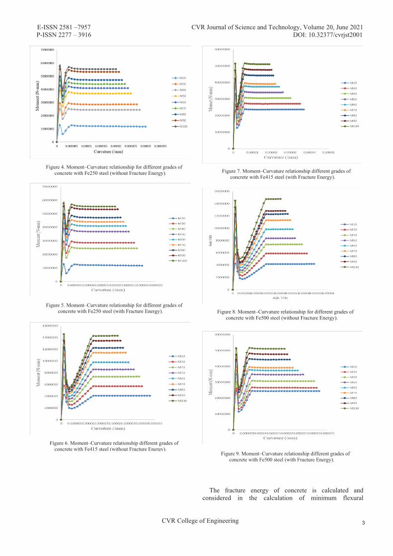
The Moment-Curvature relationships for different grades of concrete and steel are presented in, Figure 4, Figure 5. Figure 6. Figure 7, Figure 8and Figure 9 respectively.
Str
Stre
s
E-ISSN 2581 –7957 CVR Journal of Science and Technology, Volume 20, June 2021 P-ISSN 2277 – 3916 DOI: 10.32377/cvrjst2001
CVR College of Engineering
The fracture energy of concrete is calculated and
considered in the calculation of minimum flexural
Figure 4. Moment–Curvature relationship for different grades of concrete with Fe250 steel (without Fracture Energy).
Figure 5. Moment–Curvature relationship for different grades of concrete with Fe250 steel (with Fracture Energy).
Figure 6. Moment–Curvature relationship different grades of concrete with Fe415 steel (without Fracture Energy).
Figure 7. Moment–Curvature relationship different grades of concrete with Fe415 steel (with Fracture Energy).
Figure 8. Moment–Curvature relationship for different grades of concrete with Fe500 steel (without Fracture Energy).
Figure 9. Moment–Curvature relationship different grades of concrete with Fe500 steel (with Fracture Energy).

E-ISSN 2581 –7957 CVR Journal of Science and Technology, Volume 20, June 2021 P-ISSN 2277 – 3916 DOI: 10.32377/cvrjst2001
CVR College of Engineering
reinforcement. In a particular grade of concrete, minimum flexural reinforcement is decreased with the increase in grade of steel. The variation is presented in Figure. 10 and Figure 11.
Figure 10. Minimum flexural reinforcement for different grades of concrete and different grades of steel without fracture energy.
Figure 11. Minimum flexural reinforcement for different grades of concrete and different grades of steel with fracture energy.
For a particular grade of concrete, the moment at first
crack, moment at first yield and the moment at ultimate shows an increase in value. The variation is presented in Figure. 12, Figure 13, Figure. 14, Figure 15, Figure 16 and Figure 17.
Figure 12. Moment at first crack for different grades of steel and different
grades of concrete without fracture energy.
Figure 13. Moment at first crack for different grades of steel and different grades of concrete with fracture energy.
Figure 14. Moment at first yield for different grades of steel and different grades of concrete without fracture energy.
Figure 15. Moment at first yield for different grades of steel and different grades of concrete with fracture energy.
0
0.1
0.2
0.3
0.4
0.5
0.6
0.7
Fe25
0Fe
415
Fe50
0
Fe25
0Fe
415
Fe50
0
Fe25
0Fe
415
Fe50
0
Fe25
0Fe
415
Fe50
0
Fe25
0Fe
415
Fe50
0
Fe25
0Fe
415
Fe50
0
Fe25
0Fe
415
Fe50
0
Fe25
0Fe
415
Fe50
0
Fe25
0Fe
415
Fe50
0
M20 M30 M40 M50 M60 M70 M80 M90 M100
0.00
0.05
0.10
0.15
0.20
0.25
0.30
0.35
0.40
0.45
Fe25
0Fe
415
Fe50
0
Fe25
0Fe
415
Fe50
0
Fe25
0Fe
415
Fe50
0
Fe25
0Fe
415
Fe50
0
Fe25
0Fe
415
Fe50
0
Fe25
0Fe
415
Fe50
0
Fe25
0Fe
415
Fe50
0
Fe25
0Fe
415
Fe50
0
Fe25
0Fe
415
Fe50
0
M20 M30 M40 M50 M60 M70 M80 M90 M100
0
2000000
4000000
6000000
8000000
10000000
12000000
14000000
16000000
Fe25
0Fe
415
Fe50
0Fe
250
Fe41
5Fe
500
Fe25
0Fe
415
Fe50
0Fe
250
Fe41
5Fe
500
Fe25
0Fe
415
Fe50
0Fe
250
Fe41
5Fe
500
Fe25
0Fe
415
Fe50
0Fe
250
Fe41
5Fe
500
Fe25
0Fe
415
Fe50
0
M20 M30 M40 M50 M60 M70 M80 M90 M100
0
10000000
20000000
30000000
40000000
50000000
60000000
Fe25
0Fe
415
Fe50
0Fe
250
Fe41
5Fe
500
Fe25
0Fe
415
Fe50
0Fe
250
Fe41
5Fe
500
Fe25
0Fe
415
Fe50
0Fe
250
Fe41
5Fe
500
Fe25
0Fe
415
Fe50
0Fe
250
Fe41
5Fe
500
Fe25
0Fe
415
Fe50
0
M20 M30 M40 M50 M60 M70 M80 M90 M100
0
2000000
4000000
6000000
8000000
10000000
12000000
14000000
16000000
Fe25
0Fe
415
Fe50
0Fe
250
Fe41
5Fe
500
Fe25
0Fe
415
Fe50
0Fe
250
Fe41
5Fe
500
Fe25
0Fe
415
Fe50
0Fe
250
Fe41
5Fe
500
Fe25
0Fe
415
Fe50
0Fe
250
Fe41
5Fe
500
Fe25
0Fe
415
Fe50
0
M20 M30 M40 M50 M60 M70 M80 M90 M100
0
10000000
20000000
30000000
40000000
50000000
60000000
Fe25
0
Fe50
0
Fe41
5
Fe25
0
Fe50
0
Fe41
5
Fe25
0
Fe50
0
Fe41
5
Fe25
0
Fe50
0
Fe41
5
Fe25
0
Fe50
0
M20 M30 M40 M50 M60 M70 M80 M90 M100

E-ISSN 2581 –7957 CVR Journal of Science and Technology, Volume 20, June 2021 P-ISSN 2277 – 3916 DOI: 10.32377/cvrjst2001
CVR College of Engineering
Figure 16. Moment at ultimate for different grades of steel and different grades of concrete without fracture energy.
Figure 17. Moment at ultimate for different grades of steel and different grades of concrete without fracture energy.
The curvature at first yield and curvature at ultimate decrease for a particular grade of concrete with increasing grade of steel as presented in Figure. 18, Figure. 19, Figure. 20 and Figure. 21.
Figure 18. Curvature at first yield for different grades of concrete and different grades of steel without fracture energy.
Figure 19. Curvature at first yield for different grades of concrete and different grades of steel with fracture energy.
Figure 20. Curvature at ultimate for different grades of steel and different grades of concrete without fracture energy.
Figure 21. Curvature at ultimate for different grades of steel and different grades of concrete with fracture energy.
Ductility Index is decreased in a particular grade of
concrete with the increase in grade of steel as presented in Figure. 22 and Figure. 23.
0
2000000
4000000
6000000
8000000
10000000
12000000
14000000
16000000Fe
250
Fe41
5Fe
500
Fe25
0Fe
415
Fe50
0Fe
250
Fe41
5Fe
500
Fe25
0Fe
415
Fe50
0Fe
250
Fe41
5Fe
500
Fe25
0Fe
415
Fe50
0Fe
250
Fe41
5Fe
500
Fe25
0Fe
415
Fe50
0Fe
250
Fe41
5Fe
500
M20 M30 M40 M50 M60 M70 M80 M90 M100
0
10000000
20000000
30000000
40000000
50000000
60000000
Fe25
0Fe
415
Fe50
0Fe
250
Fe41
5Fe
500
Fe25
0Fe
415
Fe50
0Fe
250
Fe41
5Fe
500
Fe25
0Fe
415
Fe50
0Fe
250
Fe41
5Fe
500
Fe25
0Fe
415
Fe50
0Fe
250
Fe41
5Fe
500
Fe25
0Fe
415
Fe50
0
M20 M30 M40 M50 M60 M70 M80 M90 M100
0
0.000002
0.000004
0.000006
0.000008
0.00001
0.000012
0.000014
0.000016
Fe25
0Fe
415
Fe50
0Fe
250
Fe41
5Fe
500
Fe25
0Fe
415
Fe50
0Fe
250
Fe41
5Fe
500
Fe25
0Fe
415
Fe50
0Fe
250
Fe41
5Fe
500
Fe25
0Fe
415
Fe50
0Fe
250
Fe41
5Fe
500
Fe25
0Fe
415
Fe50
0
M20 M30 M40 M50 M60 M70 M80 M90 M100
0
0.000001
0.000002
0.000003
0.000004
0.000005
0.000006
0.000007
0.000008
Fe25
0Fe
415
Fe50
0Fe
250
Fe41
5Fe
500
Fe25
0Fe
415
Fe50
0Fe
250
Fe41
5Fe
500
Fe25
0Fe
415
Fe50
0Fe
250
Fe41
5Fe
500
Fe25
0Fe
415
Fe50
0Fe
250
Fe41
5Fe
500
Fe25
0Fe
415
Fe50
0
M20 M30 M40 M50 M60 M70 M80 M90 M100
0
0.000005
0.00001
0.000015
0.00002
0.000025
0.00003
0.000035
0.00004
Fe25
0Fe
415
Fe50
0Fe
250
Fe41
5Fe
500
Fe25
0Fe
415
Fe50
0Fe
250
Fe41
5Fe
500
Fe25
0Fe
415
Fe50
0Fe
250
Fe41
5Fe
500
Fe25
0Fe
415
Fe50
0Fe
250
Fe41
5Fe
500
Fe25
0Fe
415
Fe50
0
M20 M30 M40 M50 M60 M70 M80 M90 M100
0
0.000005
0.00001
0.000015
0.00002
0.000025
0.00003
0.000035
Fe25
0Fe
415
Fe50
0Fe
250
Fe41
5Fe
500
Fe25
0Fe
415
Fe50
0Fe
250
Fe41
5Fe
500
Fe25
0Fe
415
Fe50
0Fe
250
Fe41
5Fe
500
Fe25
0Fe
415
Fe50
0Fe
250
Fe41
5Fe
500
Fe25
0Fe
415
Fe50
0
M20 M30 M40 M50 M60 M70 M80 M90 M100

E-ISSN 2581 –7957 CVR Journal of Science and Technology, Volume 20, June 2021 P-ISSN 2277 – 3916 DOI: 10.32377/cvrjst2001
CVR College of Engineering
V. CONCLUSIONS
A programme in C-language was developed to find Moment-Curvature relationships, minimum flexural reinforcement and ductility properties of beams considering Fracture energy. 1. In a particular grade of steel, the moment at first yield increased with increase in grade of concrete. This may be due to increased strength and stiffness of the member with increase in grade of concrete. 2. It is found that, in a particular grade of concrete, the minimum flexural reinforcement decreased with the increase in grade of steel. This may be due to the increase in yield strength of steel with increase in grade of steel. 3. In a particular grade of steel, ductility index decreased with the increase in grade of concrete. This may be due to the increase in brittleness of concrete with the increase in the grade of concrete. 4. Higher the ductility index, higher the energy absorption capacity and vice versa. Therefore, the fracture energy of concrete need to be calculated accurately and should be considered in the calculation of minimum flexural reinforcement.
REFERENCES
[1] G. Kaklauskas & M. Hallgren, “Curvature Analysis of High Strength Concrete Beams”, ISSN: 1392-1525, pp 357-363,2012.
[2] Viktor Gribniak, Ieva Misiunait, Arvydas Rimkus, Aleksandr Sokolov and Antanas Šapalas, “Deformations of FRP–Concrete Composite Beam: Experiment and Numerical Analysis”, Appl. Sci, pp 2, 2019.
[3] Tejaswini V. Jadhav, V. D. Gundakalle, “Effect of Medium to High Grade of Concrete and Depth on Moment Curvature Relationship for Reinforced Concrete Beams Section”, IJSRD, Vol. 3, Issue 06, 2015.
[4] Ravi Kumar, Vimal Choudhary, K. S. Babu Narayan and D. Venkat Reddy, “Moment Curvature Characteristics for Structural Elements of RC Building”, June 22, 2014.
[5] Mohammed Fakhruddin Momin, Prashant Barbude, Kunal Bhagat, Prashant V. Muley, “Moment Curvature Relationship for Structural Elements of RC Building Using Matlab”, ISSN (Online): 2347 - 2812, Volume-5, Issue -2, 2017.
[6] Zeyang Sun, Yang Yang, Wenlong Yan, Gang Wu, and Xiaoyuan He, “Moment-Curvature Behaviours of Concrete Beams Singly Reinforced by Steel-FRP Composite Bars”, 2017.
[7] H. Barros, C. Ferreira, and T. Marques, “Moment-Curvature Diagrams for Evaluation of Second Order Effects In RC Elements”, ECCOMAS Congress, 2016.
[8] Daskshina Mirthy, Sudheer Reddy, “Moment-Curvature Characteristics of Ordinary Grade Fly Ash Concrete Beams”, International journal of civil and structural engineering, 2010.
[9] Ravi Kumar et al, “Moment- Curvature characteristics for structural elements of RC buildings”, Journal on Todays Idea-Tomorrow’s Technology, vol 2, June 2014.
[10] Hyo- gyong, Kwak, Sun-Pil Kim, “Non-linear analysis of RC beams based on Moment-Curvature Relation”, Computers and structures, 2002.
[11] M. Srikanth et al, “Moment-curvature of RC beams using various confinement models and experimental validation”, Asian Journal of Civil Engineering, 2007.
[12] D. H. Travis, G. Giongo, P. Paultre, “Behaviour of Reinforced Concrete Beams Reinforced with GFRP Beam” Ibracon Structures and Material Journal, 2008.
[13] Mohd Al Amin, Md Abur, “Effect of Material Properties on Ductility of Reinforced Concrete Beams”, The Institute of Malaysia, 2006.
[14] Abdel Hamid Charif, Saleh Dghaither, “Ductility of Reinforced Lightweight Concrete Beams Singly Reinforced by Steel FRP Composite Bars”, Advanced Civil Engineering, 2017.
[15] Gurey Arslan, Ercan Cihanli, “Curvature-Ductility Prediction of High-Strength Concrete Beams Sections”, Journals of Civil Engineering and Management,2010.
[16] Young Jang, Hoon Gyu- Park, Siu Foo Kim, “On Ductility of High Strength Concrete Beams”, International Journal of Concrete Structures and Materials, 2008.
[17] Japan society of Civil Engineers (JSCE), “Standard Specification for Concrete Structure: No 15” Cl. 13.4.2, 2007.
Figure 22. Ductility Index for a particular grade of concrete with varying grade of steel without fracture energy.
Figure 23. Ductility Index for a particular grade of concrete with varying grade of steel with fracture energy.

E-ISSN 2581 –7957 CVR Journal of Science and Technology, Volume 20, June 2021 P-ISSN 2277 – 3916 DOI: 10.32377/cvrjst2001
CVR College of Engineering
SYMBOLS
x Depth of neutral axis Ꜫcepsl Strain in Concrete fiber Ꜫs Strain in Steel ϕu curvature at failure for beam under
loading ϕc curvature at first yield for beam under
loading μ flexural ductility or curvature ductility Es Modulus of elasticity of steel Ec Modulus of elasticity of concrete
fck Characteristic compressive strength of concrete
fy Yield strength of steel St Stress in ith strip of the beam section Ro Minimum percentage of reinforcement
steel b Breath of the beam d Width of the beam l Length of the beam
E-ISSN 2581 – 7957 CVR Journal of Science and Technology, Volume 20, June 2021 P-ISSN 2277 – 3916 DOI: 10.32377/cvrjst2002
CVR College of Engineering
Role of Multiple Liquid Tuned Mass Dampers in Tall Buildings
M. Mahesh1 and Dr. N. Murali Krishna2 1Junior Engineer, Vishwa Teja Constructions/Attapur, Hyderabad, India
Email: [email protected] 2Professor, CVR College of Engineering/Civil Engg. Department, Hyderabad, India
Email: [email protected]
Abstract: High raised buildings with plan asymmetry are highly vulnerable to seismic induced vibrations on account of 1) large amount of base shear, 2) large lateral displacement and 3) twist of each story. The asymmetry in the building plan can’t be compromised due to the architectural requirements and the buildings utilities. Many techniques are attempted to minimize the base shear, lateral displacement and the twist using methods such as base isolation techniques, tuned massed dampers and the liquid tuned mass dampers. However, though the attempts are found to be fruitful, they are expensive, un acceptable and sometimes not feasible.
In this study the liquid tuned mass dampers are found more suitable and which are modeled making use of the overhead water tanks in buildings. The effect of Multiple Liquid Tuned Mass Dampers on the unsymmetrical buildings is to be studied in the present work. The study is carried-out on L-shape building, T-shape building and U-shape and rectangular building of 10, 15 stories height in different seismic zones using E-Tabs. The structural analysis is to be carried using linear time history analysis. It was found that with the increase in number of water head tanks and dampers, the base shear increased, but displacement decreased.
Index Terms: Tall structures, tuned mass damper (TMD), Tuned Liquid Mass Damper (TLMD), Base shear, Water tank, Seismic vibrations.
I. INTRODUCTION
For growing population, the only solution for accommodation remains vertical expansion, when horizontal expansion is limited. High structures pose greater challenges to structural engineer in form of stability and safety. High density tall buildings are vulnerable to lateral forces like wind forces and earthquakes. Lateral displacements at foundation level prove much risk to a buildings stability and pose threat to lives. Hence it becomes a necessity to increase stiffness and improve the structural configuration of buildings to overcome these hurdles.
The introduction of Tuned Mass Damper proved to be highly effective in reduction of base shear and amplitude of vibrations subjected to lateral forces and displacements. These also proved to be economical amongst which the usage of Liquid Tuned Mass Dampers is even more desirable due to their relative advantages. Overhead water tanks then serve as Liquid Tuned Mass Damper, which are economical and serve effectively in control of this distress.
In the present study, the mass of water in the tank plus the mass of the water tank is considered to constitute the total mass of the Tuned Mass Damper. The stiffness of the columns of the water tank would serve as the stiffness of the
Tuned Mass Damper. The structural damping due to the concrete structure constitute the damping of the Tuned Mass Damper. By suitably altering the mass of liquid in the water tank, the sizes of the water tank and the number and size of the column elements supporting the water tank, the mass, the damping and the stiffness of the Tuned Liquid Damper are tuned.
A. Objective of the study My predecessor had carried-out studies on the
contributions of single liquid tuned mass dampers. In the present work, the studies are extended to investigate the additional contributions due to multiple liquid tuned mass dampers. Having already appreciated the need to introduce multiple liquid tuned mass dampers, the present work is taken-up with following objectives: 1. To suitably choose the size of the water tank, mass of the
water tank with water as a ratio of mass of the structureand the number and sizes of the columns supporting thewater tank to arrive at an optional configuration of theLiquid Tuned Mass Damper.
2. Proposing either single or multiple numbers of LiquidTuned Mass Dampers together with their locations and allparameters as described in objective no.1.
3. The overall arrangement should result in the lowestpossible base shear and lateral displacement, yeteconomical in the event of seismic disturbance to thebuilding.
B. Procedure Adopted In this current project, ETABS package has been utilized
for Response Spectrum method and Time History analysis are on a RCC building subjected to seismic load. A G+10 and G+15 storey building, with and without Liquid Tuned Mass Dampers, located in zone–III and zone–IV of seismic disturbances is considered. L–shaped, T-shaped, U–shaped and rectangular buildings are considered. The studies are repeated by varying the water level in tanks as empty, one-third full, two-third full and full water tank conditions and the locations of the water tanks are altered to result in optimum values of seismic disturbances.
II. LITERATURE REVIEW
Chidige Anil Kumar and E Arunakranthi, the aim of the present work is analyzing the feasibility of implementing water tank as passive TMD and finding the optimum level of water which would reduce the peak response of the structure

E-ISSN 2581 – 7957 CVR Journal of Science and Technology, Volume 20, June 2021 P-ISSN 2277 – 3916 DOI: 10.32377/cvrjst2002
CVR College of Engineering
subjected to seismic force using SAP2000. The idea of seismic response control of the structures by using TMD’s is considered for this study. The frequency of the damper is tuned to a particular structural frequency so that when that frequency is excited, the damper will resonate out of phase with the structural motion and energy is dissipated by the damper inertia force acting on the structure. The building using 1893:2002, it was found that the roof displacements, storey drifts, time period and base shear have been reduced for 2/3rd level of water tank compared to other levels. It was concluded by them that if the water level of water in the tank is maintained between half full to two third full there is tendency to mitigate the vibrations of RC frame structures under seismic excitations [1].
Dorothy Reed et al analyzed Time histories of the base shear force and water-surface variations by shaking table tests and compared with a numerical model investigating behavior of tuned liquid dampers (TLD) with the help of laboratory experiment and numerical modelling. It was found that the response frequency of tuned liquid dampers increased as excitation amplitude increased, and the TLD behaved as a hardening spring system. The design frequency damper should be set at the value lower than that of the structure response frequency if it is computed using the linearized water-wave theory by which the actual nonlinear frequency of the damper matched with the structural response. It was found that, even if the damper frequency had been mistuned slightly, the TLD always performed favorably [2].
M. J. Tait, N. Isyumov investigated the performance of unidirectional and directional tuned liquid dampers (TLDs) under random excitation. A series of experiments were carried- out on scale model structure tuned liquid dampers systems for which the results are compared with those of a well-known tuned mass damper. The effective damping was calculated for each test conducted and the efficiency and robustness were subsequently examined. The performance of a mistuned TLD was experimentally investigated to highlight the robustness of these passive dynamic vibration absorbers. A nonlinear numerical model was used to conduct an extensive parametric study on the performance of a tuned liquid damper. It was concluded that a TLD is efficient and robust to reduce dynamic structural motions that occur as a result of random excitation [3].
Mudabbir Imran, Dr. B. K. Raghu Prasad Examined the effectiveness of both single and multiple tuned mass dampers (TMDs) to ease translational vibration when subjected to various earthquake ground accelerations. Making use of ETABS, they had modelled frame with single TMD, frame with multiple TMDs and a shear building with single TMD. Four external loading conditions were considered and the time history analysis was carried out for appropriate ground motion. The variations of displacements in the structural were compared. It was found that the response of the frame structure in terms of displacement reduced with the increase in the mass ratio of the single TMD. It has been observed that a frame structure equipped with MTMD with uniform distribution of mass ratio was more effective in controlling the vibrations of the structure compared to STMD as multiple dampers can weaken different modes. From the frames equipped with MTMD with uniform and non- uniform mass
ratios it was seen that MTMD with Non- uniform mass ratio was more efficient than MTMD with uniform mass ratio [4].
III. METHODOLOGY
The dynamic analysis of the building is carried out using Response Spectrum method Linear Time History method corresponding to seismic Zones-III and IV of seismic activities.
Modelling of structure using TLD is as follows: 1. A three-dimensional model of G+10 and G+15 Stories
building Structure is created using ETABS. 2. Created and assigning Material Properties. 3. Created and assigning Section Properties. 4. Response Spectrum and Time History functions are
defined for the desired zones considered in the study. 5. Assigning the external and internal wall loads acting on
the structure wherever necessary. 6. Assigning the floor finish load and live load acting on slab
panels. 7. A water tank is created at the desired location on the top
most of the existing building structure. 8. The water tank with desired length, width and height are
created and the beam, column and slab properties are assigned.
9. The next step is modelling a Tuned Liquid Damper which is attached to the water tank of the same building.
10. A TLD is modelled in ETABS using a combination of ‘Linear link type’ and a ‘Point spring’ attached in series.
11. From the Define� Section Properties� Link/support properties, add a new link property, add a new link property by selecting the ‘Linear link type’. The directional properties U1, U2, and U3 are selected in which U3 type is fixed.
12. From properties option�modify/show all�the stiffness and damping values for U1, U2 directions are entered.
13. Mass weight of the TLD (the water) is entered, which is the load acting on the water tank or the weight of water present in the water tank. In this step, the water level is varied to effect the changes in the values of mass weight of TLD and changes are in the stiffness and damping as well.
14. Define�Spring properties�point springs�Add new spring, select the ‘User specified/link properties option’.
15. From the ‘single joints link at point’ dialogue box, add the previous defined link property and the axial direction ‘+Z’ selected.
16. Links are drawn using ‘draw link’ option. 17. The links are connected to the columns in ‘+z’ direction
(upward), along which the water tank is standing. 18. The point spring which is defined earlier is assigned to the
joints at the base of the water tank by using ‘Draw spring’ option.
19. The mass of the TLD is assigned towards the free end of the link by selecting the joints of water tank, where springs and links are connected.
20. From the command Assign�Joint loads, the load value is assigned in downward or ‘-z’ direction. The total load acting on the water tank is divided equally on to the number of columns on which it is standing as shown figure 1.

E-ISSN 2581 – 7957 CVR Journal of Science and Technology, Volume 20, June 2021 P-ISSN 2277 – 3916 DOI: 10.32377/cvrjst2002
CVR College of Engineering
Figure 1. Plan with joint loads in ETABS The buildings considered for the study are RC ordinary
moment resisting space frames of G+10 and G+15 storey located in zone-III and IV of seismic disturbances. The analysis is carried-out on a rectangular shaped building and three different asymmetric shaped buildings of plan shapes L, T and U. The study is conducted by varying the water level in water tank by considering, 1. Empty water tank, 2. One-third, 3. Two-third’s full and 4. Full water tank conditions using ETABS software.
The Plan configurations of G+10, One water tank.
1. Model 1 - L-shaped plan Building (Figure 2), 2. Model 2 - T-shaped plan Building (Figure 3), 3. Model 3 - U-shaped plan Building (Figure 4), 4. Model 4 - Building Rectangular plan (Figure 5),
Figure 2. Plan and Isometric view of Model-1 with TLD
Figure 3. Plan and Isometric view of Model-2 with TLD
Figure 4. Plan and Isometric view of Model-3 with TLD
Figure 5. Plan and Isometric view of Model-4 with TLD
The Plan configurations of G+10, Two water tank.
1. Model 5 - L-shaped plan Building (Figure 6), 2. Model 6 - T-shaped plan Building (Figure 7), 3. Model 7 - U-shaped plan Building (Figure 8), 4. Model 8 - Building Rectangular plan (Figure 9),
Figure 6. Plan and Isometric view of Model-5 with TLD
Figure 7. Plan and Isometric view of Model-6 with TLD
Figure 8. Plan and Isometric view of Model-7 with TLD

E-ISSN 2581 – 7957 CVR Journal of Science and Technology, Volume 20, June 2021 P-ISSN 2277 – 3916 DOI: 10.32377/cvrjst2002
CVR College of Engineering
Figure 9. Plan and Isometric view of Model-8 with TLD
The Plan configurations of G+10, Three water tank.
1. Model 9 - L-shaped plan Building (Figure 10), 2. Model 10 - T-shaped plan Building (Figure 11), 3. Model 11 - U-shaped plan Building (Figure 12), 4. Model 12 - Building Rectangular plan (Figure 13),
Figure 10. Plan and Isometric view of Model-9 with TLD
Figure 11. Pan and Isometric view of Model-10 with TLD
Figure 12. Plan and Isometric view of Model-11 with TLD
Figure 13. Plan and Isometric view of Model-12 with TLD
The Plan configurations of G+15, One water tank.
1. Model 13 - L-shaped plan Building (Figure 14), 2. Model 14 - T-shaped plan Building (Figure 15), 3. Model 15 - U-shaped plan Building (Figure 16), 4. Model 16 - Building Rectangular plan (Figure 17),
Figure 14. Plan and Isometric view of Model-13 with TLD
Figure 15. Plan and Isometric view of Model-14 with TLD
Figure 16. Plan and Isometric view of Model-15 with TLD
Figure 17. Plan and Isometric view of Model-16 with TLD
The Plan configurations of G+15, Two water tank.
1. Model 17 - L-shaped plan Building (Figure 18), 2. Model 18 - T-shaped plan Building (Figure 19), 3. Model 19 - U-shaped plan Building (Figure 20), 4. Model 20 - Building Rectangular plan (Figure 21),
Figure 18. Plan and Isometric view of Model-17 with TLD

E-ISSN 2581 – 7957 CVR Journal of Science and Technology, Volume 20, June 2021 P-ISSN 2277 – 3916 DOI: 10.32377/cvrjst2002
CVR College of Engineering
Figure 19. Plan and Isometric view of Model-18 with TLD
Figure 20. Plan and Isometric view of Model-19 with TLD
Figure 21. Plan and Isometric view of Model-20 with TLD
The Plan configurations of G+15, Three water tank.
1. Model 21 - L-shaped plan Building (Figure 22), 2. Model 22 - T-shaped plan Building (Figure 23), 3. Model 23 - U-shaped plan Building (Figure 24), 4. Model 24 -Building Rectangular plan (Figure 25),
Fig 22. Plan and Isometric view of Model-21 with TLD
Figure 23. Plan and Isometric view of Model-22 with TLD
Figure 24. Plan and Isometric view of Model-23 with TLD
Figure 25. Plan and Isometric view of Model-24 with TLD
IV. SPECIEMN CALCULATIONS
The preliminary data for the Analysis of the frame in ETABS is considered as per the prevailing construction practice which is presented below.
1. Type of structure - Moment Resisting Frame 2. Materials -M30. Fe-500 3. Size of Beams -300x450 mm 4. Size of Columns -450x750 mm 5. Depth of Slab -150 mm 6. External Wall Load -11.14KN/m (IS 875 Part-1) 7. Internal Wall Load -5.57KN/m (IS 875 Part-1) 8. Seismic zone factor -0.16 & 0.24 (IS893:2016) 9. Response Reduction Factor -5 (IS 1893-2016)
A. Calculations of water tank for Model-L Total mass of the structure = 70209.18KN
Water required for single person = 135 liters No. of persons in each flat = 5 No. of flats in the building = 25 Total no of persons = 125 Water required = 16875 Water tank height = 0.75 m Volume of tank = LxBxH Area of tank (LxB) = 22.5 m2 L = 6 m B = 6 m H = 0.75 m
Total dead load =530.82KN Live Load (Water Required) = 165.48 KN
Total water tank load = 697.05KN
B. Calculations of the Tuned Liquid Damper for Model-L
Mass ratio (γ) =
Natural frequency (ωn) =1.874rad/sec

E-ISSN 2581 – 7957 CVR Journal of Science and Technology, Volume 20, June 2021 P-ISSN 2277 – 3916 DOI: 10.32377/cvrjst2002
CVR College of Engineering
Time period (Tn) =3.351 sec
*Tuning ratio (fopt) =
*Optimum damping ratio (ξdopt) =
*Optimum stiffness Kopt = γkfopt
2 *Optimum Damping Copt = 2ωmξdoptγ The above calculations are listed below in Table-1
TABLE I. CALCULATIONS OF TLMD PARAMETERS FOR VARYING WATER LEVEL IN
THE TANK Empty
Water tank
One-third level Water
Two-third level water
Full water tank
Mass ratio 0 0.00330 0.0066
0.00992
Tuning ratio 1 0.996
0.993
0.9901
Optimum damping ratio
0 0.03528
0.0499
0.0613
Optimum stiffness (KN/m)
0 82.72
164.371
244.94
Optimum Damping (KN-s/m)
0 30.74
87.09 160.26
V. RESULTS AND DISCUSSIONS
After analyzing the RCC buildings of ten-storey and fifteen-storey high using both Response Spectrum and Linear Time History Analysis methods with and without TLD’s, the results obtained in respect of base shear and maximum storey displacement in two orthogonal directions are tabulated in Tables. The studies are carried-out with water tank empty, one-third full, two-third full and full.
A. Zone-III, ten storey building 1. L-Shaped buildings of ten-storey high with one water
tank, when dampers are introduced, the base shear has slightly increased when tanks carry more water as compared to the tank without dampers. But the maximum displacement reduced by 43% when dampers are introduced.
2. L-Shaped building of ten-storey high with TWO water tanks, when dampers are introduced, the base shear has slightly increased when tanks are filled as compared to the tanks without dampers, but the maximum displacement was 58% less when dampers are introduced.
3. L-Shaped building of ten-storey high with THREE water tanks, when dampers are introduced, the base shear has slightly increased when tanks are filled as compared to the tanks without dampers, but the maximum displacement was 63% less when dampers are introduced.
4. T-Shaped building of ten-storey high with ONE water tank, when dampers are introduced, the base shear has slightly increased when tanks are filled as compared to the tank without dampers, but the maximum displacement was 43% less when dampers are introduced.
5. T-Shaped building of ten-storey high with TWO water tanks, when dampers are introduced, the base shear has slightly increased when tanks are filled as compared to the tanks without dampers, but the maximum displacement was 55% less when dampers are introduced.
6. T-Shaped building of ten-storey high with THREE water tanks, when dampers are introduced, the base shear has slightly increased when tanks are filled as compared to the tanks without dampers, but the maximum displacement was 58% less when dampers are introduced.
7. U-Shaped building of ten-storey high with ONE water tank, when dampers are introduced, the base shear has slightly increased when tanks are filled as compared to the tank without dampers, but the maximum displacement was 24% less when dampers are introduced.
8. U-Shaped building of ten-storey high with TWO water tanks, when dampers are introduced, the base shear has slightly increased when tanks are filled as compared to the tanks without dampers, but the maximum displacement was 41% less when dampers are introduced.
9. U-Shaped building of ten-storey high with THREE water tanks, when dampers are introduced, the base shear has increased when tanks are filled as compared to the tanks without dampers, but the maximum displacement was 47% less when dampers are introduced.
10. Rectangular-Shaped building of ten-storey high with ONE water tank, when dampers are introduced, the base shear has decreased when tanks are filled as compared to the tank without dampers, but the maximum displacement was 18% less when dampers are introduced.
11. Rectangular-Shaped building of ten-storey high with TWO water tanks, when dampers are introduced, the base shear has decreased when tanks are filled as compared to the tanks without dampers, but the maximum displacement was 34% less when dampers are introduced.
12. Rectangular-Shaped building of ten-storey high with THREE water tanks, when dampers are introduced, the base shear has slightly decreased when tanks are filled as compared to the tanks without dampers, but the maximum displacement was 42% less when dampers are introduced.
B. Zone-IV, ten storey building 13. L-Shaped building of ten-storey high with ONE water
tank, when dampers are introduced, the base shear has slightly increased when tanks are filled as compared to the tank without dampers, but the maximum displacement was 42% less when dampers are introduced.
14. L-Shaped building of ten-storey high with TWO water tanks, when dampers are introduced, the base shear has slightly increased when tanks are filled as compared to the tanks without dampers, but the maximum displacement was 58% less when dampers are introduced.
15. L-Shaped building of ten-storey high with THREE water tanks, when dampers are introduced, the base shear has slightly increased when tanks are filled as compared to the tanks without dampers, but the maximum displacement was 63% less when dampers are introduced.
16. T-Shaped building of ten-storey high with ONE water tank, when dampers are introduced, the base shear has

E-ISSN 2581 – 7957 CVR Journal of Science and Technology, Volume 20, June 2021 P-ISSN 2277 – 3916 DOI: 10.32377/cvrjst2002
CVR College of Engineering
slightly increased when tanks are filled as compared to the tank without dampers, but the maximum displacement was 44% less when dampers are introduced.
17. T-Shaped building of ten-storey high with TWO water tanks, when dampers are introduced, the base shear has slightly increased when tanks are filled as compared to the tanks without dampers, but the maximum displacement was 55% less when dampers are introduced.
18. T-Shaped building of ten-storey high with THREE water tanks, when dampers are introduced, the base shear has increased when tanks are filled as compared to the tanks without dampers, but the maximum displacement was 58% less when dampers are introduced.
19. U-Shaped building of ten-storey high with ONE water tank, when dampers are introduced, the base shear has slightly increased when tanks are filled as compared to the tank without dampers, but the maximum displacement was 24% less when dampers are introduced.
20. U-Shaped building of ten-storey high with TWO water tanks, when dampers are introduced, the base shear has slightly increased when tanks are filled as compared to the tanks without dampers, but the maximum displacement was 41% less when dampers are introduced.
21. U-Shaped building of ten-storey high with THREE water tanks, when dampers are introduced, the base shear has slightly increased when tanks are filled as compared to the tanks without dampers, but the maximum displacement was 47% less when dampers are introduced.
22. Rectangular-Shaped building of ten-storey high with ONE water tank, when dampers are introduced, the base shear has decreased when tanks are filled as compared to the tank without dampers, but the maximum displacement was 18% less when dampers are introduced.
23. Rectangular-Shaped building of ten-storey high with TWO water tanks, when dampers are introduced, the base shear has decreased when tanks are filled as compared to the tanks without dampers, but the maximum displacement was 34% less when dampers are introduced.
24. Rectangular-Shaped building of ten-storey high with THREE water tanks, when dampers are introduced, the base shear has slightly decreased when tanks are filled as compared to the tanks without dampers, but the maximum displacement was 42% less, when dampers are used.
C. Zone-III, fifteen storey building 1. L-Shaped building of fifteen storey high with ONE water
tank, when dampers are introduced, the base shear has slightly decreased when tanks are filled as compared to the tank without dampers, but the maximum displacement was 49% less when dampers are introduced.
2. L-Shaped building of fifteen-storey high with TWO water tanks, when dampers are introduced, the base shear has slightly increased when tanks are filled as compared to the tanks without dampers, but the maximum displacement was 63% less when dampers are introduced.
3. L-Shaped building of fifteen storey high with THREE water tanks, when dampers are introduced, the base shear has slightly increased when tanks are filled as compared to the tanks without dampers, but the maximum displacement was 68% less when dampers are introduced.
4. T-Shaped building of fifteen-storey high with ONE water tank, when dampers are introduced, the base shear has slightly decreased when tanks are filled as compared to the tank without dampers, but the maximum displacement was 50% less when dampers are introduced.
5. T-Shaped building of fifteen storey high with TWO water tanks, when dampers are introduced, the base shear has slightly decreased when tanks are filled as compared to the tanks without dampers, but the maximum displacement was 61% less when dampers are introduced.
6. T-Shaped building of fifteen storey high with THREE water tanks, when dampers are introduced, the base shear has slightly increased when tanks are filled as compared to the tanks without dampers, but the maximum displacement was 64% less when dampers are introduced.
7. U-Shaped building of fifteen storey high with ONE water tank, when dampers are introduced, the base shear has slightly decreased when tanks are filled as compared to the tank without dampers, but the maximum displacement was 30% less when dampers are introduced.
8. U-Shaped building of fifteen storey high with TWO water tanks, when dampers are introduced, the base shear has slightly decreased when tanks are filled as compared to the tanks without dampers, but the maximum displacement was 49% less when dampers are introduced.
9. U-Shaped building of fifteen storey high with THREE water tanks, when dampers are introduced, the base shear has decreases when tanks are filled as compared to the tanks without dampers, but the maximum displacement was 55% less when dampers are introduced.
10. Rectangular-Shaped building of fifteen storey high with ONE water tank, when dampers are introduced, the base shear has decreased when tanks are filled as compared to the tank without dampers, but the maximum displacement was 29% less when dampers are introduced.
11. Rectangular-Shaped building of fifteen storey high with TWO water tanks, when dampers are introduced, the base shear has slightly decreased when tanks are filled as compared to the tanks without dampers, but the maximum displacement was 43% less when dampers are introduced.
12. Rectangular-Shaped building of fifteen storey high with THREE water tanks, when dampers are introduced, the base shear has slightly increased when tanks are filled as compared to the tanks without dampers, but the maximum displacement was 48% less when dampers are introduced.
D. Zone-IV, fifteen storey building 13. L-Shaped building of fifteen storey high with ONE water
tank, when dampers are introduced, the base shear has slightly reduced when tanks are filled as compared to the tank without dampers, but the maximum displacement was 49% less when dampers are introduced.
14. L-Shaped building of fifteen storey high with TWO water tanks, when dampers are introduced, the base shear has slightly increased when tanks are filled as compared to the tanks without dampers, but the maximum displacement was 63% less when dampers are introduced.
15. L-Shaped building of fifteen storey high with THREE water tanks, when dampers are introduced, the base shear has slightly increased when tanks are filled as compared
E-ISSN 2581 – 7957 CVR Journal of Science and Technology, Volume 20, June 2021 P-ISSN 2277 – 3916 DOI: 10.32377/cvrjst2002
CVR College of Engineering
to the tanks without dampers, but the maximum displacement was 68% less when dampers are introduced.
16. T-Shaped building of fifteen storey high with ONE water tank, when dampers are introduced, the base shear has slightly reduced when tanks are filled as compared to the tank without dampers, but the maximum displacement was 50% less when dampers are introduced.
17. T-Shaped building of fifteen storey high with TWO water tanks, when dampers are introduced, the base shear has slightly reduced when tanks are filled as compared to the tanks without dampers, but the maximum displacement was 61% less when dampers are introduced.
18. T-Shaped building of fifteen storey high with THREE water tanks, when dampers are introduced, the base shear has slightly increased when tanks are filled as compared to the tanks without dampers, but the maximum displacement was 64% less when dampers are introduced.
19. U-Shaped building of fifteen storey high with ONE water tank, when dampers are introduced, the base shear has slightly reduced when tanks are filled as compared to the tank without dampers, but the maximum displacement was 30% less when dampers are introduced.
20. U-Shaped building of fifteen storey high with TWO water tanks, when dampers are introduced, the base shear has slightly reduced when tanks are filled as compared to the tanks without dampers, but the maximum displacement was 49% less when dampers are introduced.
21. U-Shaped building of fifteen storey high with THREE water tanks, when dampers are introduced, the base shear has slightly reduced when tanks are filled as compared to the tanks without dampers, but the maximum displacement was 55% less when dampers are introduced.
22. Rectangular-Shaped building of fifteen storey high with ONE water tank, when dampers are introduced, the base shear has slightly reduced when tanks are filled as compared to the tank without dampers, but the maximum displacement was 29% less when dampers are introduced.
23. Rectangular-Shaped building of fifteen storey high with TWO water tanks, when dampers are introduced, the base shear has slightly reduced when tanks are filled as compared to the tanks without dampers, but the maximum displacement was 43% less when dampers are introduced.
24. Rectangular-Shaped building of fifteen storey high with THREE water tanks, when dampers are introduced, the base shear has slightly increased when tanks are filled as compared to the tanks without dampers, but the maximum displacement was 51% less when dampers are introduced.
VI. CONCLUSIONS
In the present work, the dynamic analysis using ETABS package is performed on 10-storey and 15-Storey RCC buildings of different plan shapes in zone-3 and zone-4, with and without tuned liquid dampers. The results pertaining to base shear and maximum floor displacements are tabulated. With the values of the base shear and maximum lateral displacements available from tables, in chapter-5, the results and discussions are documented. Finally, based on the results and discussions, following conclusions are drawn.
1. Introduction TLD modelling of water tanks have invariably reduced the magnitudes of base shear and maximum lateral displacements to an extent of twenty percent.
2. Increasing water levels in the tanks, with either single or multiple TLD’s have resulted in the marginal increase in base shear but substantial decrease the maximum lateral displacements for RCC buildings with L shaped plans.
3. A similar behaviour is noticed for buildings with rectangular, T shaped and U-shaped plans as well.
4. Even though the magnitudes of base shear and maximum lateral displacement increase are higher for zone-4 in relation to zone-3, the magnitudes of base shear and maximum lateral displacements have exhibited a similar trend.
5. The structural design of high raised RCC buildings with multiple water tanks is most economical when the water tanks are modelled as TLDs. For design purpose, the maximum values of base shear and maximum lateral displacements shall be considered based on the quantum of water in tanks.
6. Even though, the sizing of water tank is decided based on the water requirements of a building, they are divided into multiple numbers to cause minimum dynamic disturbance to the building, in the event of seismic activity.
A. Scope for future work As of now, a large amount of information is available
regarding the base shear and the maximum lateral displacement for RCC buildings of different heights, different seismic zones, and different shapes of plans both with and without TLDs. This large data set may be used to train a neural net using back propagation paradigm. The input layer of the neural net would contain the shape of the building, numbers of stories, seismic zone coefficient, and number of TLDs, the relative fullness of tanks, Mass/Damping/Stiffness information of TLDs and their location with respect to mass center of the building in plan. The outputs of the net shall be the base shear and maximum lateral displacement. Such a trained neural net would recommend optimum configuration of numbers of TLD’s, their locations in building plan and their capacities.
REFERENCES [1] Chidige Anil Kumar, E Arunakanthi “A Seismic Study on
Effect of Water Tank modelled as Tuned Mass Damper”, International Journal of Innovation Research in Science, Engineering and Technology (2017).
[2] Dorothy Reed, Jinkyu Yu, z Harry Yes, Sigurdur Gardarsson “Investigation of Tuned Liquid Dampers under Large Amplitude Excitation”, American Society of Civil Engineers (1998).
[3] M. J. Tait, N. Isyumov, A. EI Damatty “Performance of Tuned Liquid Dampers”, American Society of Civil Engineers (2008).
[4] Mudabbir Imron, Dr. B. K. Raghu prasad “Seismic Response of Tail Structure Using Tuned Mass Dampers”, International Journal of Research in Engineering and Applied Science (2017).
[5] A. Lucchini, R. Greco, G. C. Marano and G. Monti “Robust Design of Tuned Mass Damper Systems for Seismic Protection

E-ISSN 2581 – 7957 CVR Journal of Science and Technology, Volume 20, June 2021 P-ISSN 2277 – 3916 DOI: 10.32377/cvrjst2002
CVR College of Engineering
of Multi-Storey Buildings”, American Society of Civil Engineers (2014).
[6] Emiliano Matta, “Effectiveness of Tuned Mass Dampers against Ground Motion Pulses”, American Society of Civil Engineers (2013).
[7] Manjusha M, Dr. Vra Saathappan “Analytical Investigation of Water Tank as Tuned Mass Damper Using Etabs”, International Research Journal of Engineering and Technology (2017).
[8] Khemraj S. Deore, Dr. Rajasekhar S. Talikoti, Kanhaiya K. Tolani “Vibration Analysis of structure using Tuned Mass Damper”, International Research Journal Engineering and Technology (2017).
[9] Ahmad Abdelraheem Fraghaly, Mahmoud Salem Ahmed “Optimum Design of Tuned Mass Damper System for Tall buildings”, International Scholarly Research Network (2012).
[10] S. M. Zahari, A. Ghannadi-Asl “Seismic Performance of Tuned Mass Dampers in Improving the Response of MRF Buildings”, Scientia Iranica (2008).
[11] Ashish A. Mohite, G.R. Patil “Earthquake Analysis of Tall Building with Tuned Mass Damper”, ISOR (2015).
[12] Saurabh Chalke, P. V. Muley “Vibration Control of Framed Structure Using Tuned Mass Damper” International Journal of Engineering Development and Research (2017).
[13] Dargush and Soong “Passive energy dissipation system for structural for design and retrofit.
[14] Fahim Sadek, Bijan Mohraz, Andrew W. Taylor and Riley M. Chung “A Method of Estimating the Parameters of Tuned Mass Dampers for Seismic Applications” (1997).
[15] Den Hartog “A Book on Mechanical Vibrations”. [16] A Shruthi, Dr. N. Murali Krishna “Role of Liquid Tuned Mass
Dampers in Improving Torsional Competence of Asymmetric Buildings” CVR Journal of Science and Technology (2019).

E-ISSN 2581 – 7957 CVR Journal of Science and Technology, Volume 20, June 2021 P-ISSN 2277 – 3916 DOI: 10.32377/cvrjst2003
CVR College of Engineering
Analysis of Reinforced Concrete Framed Structure Subjected to Blast Load sing Sap2000
Mittakolu Harveen Sai PG Scholar, CVR College of Engineering/Civil Engg. Department, Hyderabad, India
Email: [email protected]
Abstract: Blast is a wave of exceedingly compressed air spreading outwards from an explosion. Blast loading is the result of an explosion where this refers to a fast and surprising launch of saved energy. Some portion of the energy is released as thermal radiation while the major component of the response is coupled into the air as air blast and into the dirt as ground stun, both as radially growing stun waves. Blast loading on buildings can be from unconfined or partially restrained explosion charges. In the present project, the main aim is to analyze the response of reinforced concrete framed structure subjected to blast loads, with external blasting stand-off distances as 10m, 20m, & 30m and with different charge weights as 100kg, 200kg, and 300kg TNT. shear wall techniques are implemented to resist the structure using IS 4991:1968. Dynamic analysis of framed structure is done by time history function method using SAP2000 software and it also includes the detail report on displacements, and story drift of structure.
Index Terms: Explosion, impact, air blast, structural response, stand-off distances, SAP2000.
I. INTRODUCTION
Blast loading is a rising threat in the world, due to an extend in global terrorism. This creates an increased danger to critical infrastructure due to blast load. The cost of building was upgrading for a “certain level” of resistance against terrorist threats. A blast explosion is immediately cause of nearby building in a catastrophic damage. Due to main fiascoes following from gas-chemical blasts outcome in enormous unique burdens, bigger than the first sketch heaps of structure by way of this building's outside and inside underlying casings, falling of dividers, extinguishing of goliath regions of windows, and closing down of fundamental life security frameworks such as fire, & smoke induced damage to structure. blast induced the impulsive loads by these loads considerations the structure can be analyzed and designed with in Indian standard limits.[8]
A. Objective: 1. A G+10 multistore commercial structure within IS456:2000 limits for section properties and IS 10262:2009 limits for concrete mix design. 2. Gravity loads are induced on structure within the Indianstandards limits. 3. By numerical calculation with respect to IS 4991:1968 blastload is applied to structure. 4. With the same intensity of blast and shear wall techniqueare used. 5. Time history function is used to analyze with blast load.
B. Scope: In order to achieve the above objectives, tasks involving computations were carried. Reinforced concrete framed structure is subjected to bast dynamic loads in FEM package SAP2000 and the effect of blast pressure on structural components was represented.
II. BACKGROUN
A. Explosion: It is an abrupt transformation of potential energy into
kinetic energy with creation of gas discharge under pressure condition. Due to sudden release of gas pressure causes an increase in temperature and material present in that pressure is converted into hot compressed gases. These gases are in high temperature and high pressure and expand rapidly without a unique direction that creates a pressure wave which is known as a shock wave. The shock wave is air is generally referred as blast wave and almost instantaneously damage the built environment.[14] i. In Chemical Explosion: Fuel or any other carbon andhydrogen atoms mixes with air or another oxidizer agent results in rapid combustion reactions and gets damage to structures and environmental creatures [3] ii. In Physical Explosion: Energy is launched from thecatastrophic failure of a compressed gasoline in cylinder, volcanic eruptions and mixing of two liquids at one-of-a-kind temperatures [3] iii. In Nuclear Explosion: Materials used to produce nuclearexplosion by fission contains isotopes of uranium and plutonium and materials used to produce nuclear explosion. [3]
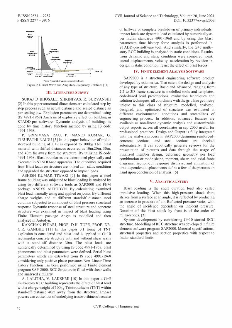
B. Blast phenomenon: When the blast occurs with respect to stand off distance to
structure, there is an increase in pressure above the ambient atmospheric pressure (Po). the pressure rapidly increases and reaches its peak value called over pressure (Pso). The pressure at that point rots into the surrounding level at time (td). After a session, the explosion at a certain distance the pressure behind the shock front decreases at that stage is called Negative Phase/ Negative phase impulse. The time duration runs in negative phase impulse is called negative duration (td
-). Later the pressure behind the shock front increases at that stage is called Positive Phase/ Positive phase impulse. The time duration runs in positive phase impulse is called Positive duration (td) as shown in Figure 2.1. [7]
E-ISSN 2581 – 7957 CVR Journal of Science and Technology, Volume 20, June 2021 P-ISSN 2277 – 3916 DOI: 10.32377/cvrjst2003
CVR College of Engineering
Figure 2.1. Blast Wave and Amplitude-Frequency Relations [12]
III. LITERATURE SURVEY
SURAJ D BHOSALE, SHRINIVAS. R. SURVANSHI [2] In this paper structural dimensions are calculated step by step process such as actual distance and scaled distance as per scaling law. Explosion parameters are determined using (IS 4991-1968) Analysis of explosive effect on building in STADD-pro software. Dynamic analysis of buildings is done by time history function method by using IS code 4991-1968.
P. SRINIVASA RAO, P. MANOJ KUMAR, G. TIRUPATHI NAIDU [3] In this paper behaviour of multi-storeyed building of G+7 is exposed to 100kg TNT blast material with shifted distances occurred as 10m,20m, 30m, and 40m far away from the structure. By utilizing IS code 4991-1968, Blast boundaries are determined physically and executed in STADD-ace apparatus. The outcomes acquired from Blast loads on structure are looked at in static condition and upgraded the structure opposed to impact loads.
ASHISH KUMAR TIWARI [5] In this paper a steel frame building was subjected to blast loading is analysed by using two different software tools as SAP2000 and FEM package ANSYS AUTODYN. By calculating examined blast load manually using and applied on joints. By different charge weights and at different standoff distance steel columns subjected to an amount of blast pressure structural response Dynamic response of steel structure and concrete structure was examined in impact of blast loading using Finite Element package Ansys is modelled and then analysed in Autodyn.
KANCHAN PUJARI, PROF. D.H. TUPE, PROF. DR. G.R. GANDHE [11] In this paper 0.1 tonne of TNT explosion is considered and blast load is applied to G+10 rectangular concrete structure with and without shear walls with a stand-off distance 30m. The blast loads are numerically determined by using IS code 4991-1968, blast phenomena and blast parameters were defined. Serial blast parameters which are extracted from IS code 4991-1968 considering only positive phase pressures Non-Linear Time history function has been performed using Finite element program SAP-2000. RCC Structure in filled with shear walls and analysed similarly.
A. LALITHA, V. LAKSHMI [10] In this paper a G+5 multi-story RCC building represents the effect of blast load with a charge weight of 100kg Trinitrotoluene (TNT) within stand-off distance 40m away from the structure. Impact powers can cause loss of underlying trustworthiness because
of halfway or complete breakdown of primary individuals. impact loads are dynamic load calculated by numerically as per Indian standards 4991-1968 and by using this blast parameters time history force analysis is performed in STADD-pro software tool. And similarly, the G+5 multi-story RCC building is analysed in static conditions. Results from dynamic and static condition were compared: peak lateral displacements, velocity, acceleration by revision in design in static condition, resist the effect of blast forces.
IV. FINITE ELEMENT ALALYSIS SOFTWARE
SAP2000 is a structural engineering software product developed by csiamerica. That caters the design and analysis of any type of structure. Basic and advanced, ranging from 2D to 3D frame structure is modelled tools and templates, code-based load prescriptions, evaluation techniques and solution techniques, all coordinate with the grid like geometry unique to this class of structure. modelled, analyzed, designed, and optimized of structure was evaluated at different environmental conditions and streamlines of engineering process. In addition, advanced features are available as non-linear dynamic analysis and customizable output reports across all coordinates in sap 2000 useful for professional practices. Design and Output is fully integrated with the analysis process in SAP2000 designing reinforced-concrete sections, and steel sections are checked automatically. It can robotically generate reviews for the presentation of pictures and data through the usage of Finalized member design, deformed geometry per load combination or mode shape, moment, shear, and axial-force diagrams, section-cut response displays, and animation of time-dependent displacements define a few of the pictures on hand upon conclusion of analysis. [5]
V. ANALYTICAL STUDY
Blast loading is the short duration load also called impulsive loading. When this high-pressure shock front strikes from a surface at an angle, it is reflected by producing an increase in pressure of air. Reflected pressure varies with the angle of incidence dependent on incident pressure. Duration of the blast shock by front is of the order of milliseconds. [2]
System development by considering G+10 storied RCC structure. Modelling of RCC structure was developed in finite element software program SAP2000. Material specifications, structural properties and section properties with respect to Indian standard limits.
E-ISSN 2581 – 7957 CVR Journal of Science and Technology, Volume 20, June 2021 P-ISSN 2277 – 3916 DOI: 10.32377/cvrjst2003
CVR College of Engineering
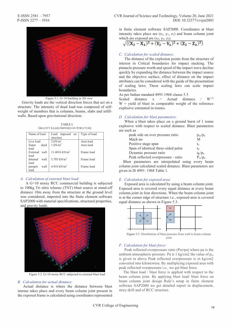
Figure 5.1. G+10 building in 3D view
Gravity loads are the vertical direction forces that act on a structure. The intensity of dead load was composed of self-weight of members that is columns, beams, slabs and infill-walls. Based upon gravitational direction.
TABLE I. GRAVITY LOADS IMPOSED ON STRUCTURE
Name of load Load imposed on structure
Type of load
Live load 2 kN/m2 Area load Super dead load
1 kN/m2 Area load
External wall load
11.4816 kN/m2 Frame load
Internal wall load
5.705 kN/m2 Frame load
parapet wall load
4.416 kN/m2 Frame load
A. Calculation of external blast load:
A G+10 storey RCC commercial building is subjected to 100kg Tri nitro toluene (TNT) blast source at stand-off distance 10m away from the structure at the ground level was considered, imported into the finite element software SAP2000 with material specifications, structural properties, and gravity loads.
Figure 5.2. G+10 storey RCC subjected to external blast load
B. Calculation for actual distance:
Actual distance is where the distance between blast intense takes place and every beam column joint present in the exposed frame is calculated using coordinates represented
in finite element software SAP2000. Coordinates at blast intensity takes place are (x1, y1, z1) and beam column joint which are exposed are (x2, y2, z2).
C. Calculation for scaled distance: The distance of the explosion points from the structure of
interest in Critical boundaries for impact stacking. The pinnacle pressure worth and speed of the impact wave decline quickly by expanding the distance between the impact source and the objective surface, effect of distance on the impact attributes can be considered with the guide of the presentation of scaling laws. These scaling laws can scale impact boundaries. As per Indian standard 4991:1968 clause 5.3 Scaled distance x = Actual distance / W1/3 W = yield of blast in comparable weight of the reference explosive estimated in tonnes. D. Calculation for blast parameters:
When a blast takes place on a ground burst of 1 tonne explosive with respect to scaled distance. Blast parameters are such as
peak side on over pressure ratio pso/pa Mach no M Positive stage span to Span of identical three-sided pulse td Dynamic pressure ratio qo/pa Peak reflected overpressure - ratio Pro/pa
Blast parameters are interpolated using every beam column joint calculated scaled distance. Blast parameters are given in IS 4991: 1968 Table 1.
E. Calculation for exposed area:
Exposed area is calculated by using a beam column joint. Exposed area is covered every equal distance at every beam column joint in four directions. When the beam column joint is at the corner edge of structure i.e., exposed area is covered equal distance as shown in Figure 5.3.
Figure 5.3. Distribution of blast pressure from wall to beam column
joint
F. Calculation for blast force: Peak reflected overpressure ratio (Pro/pa) where pa is the
ambient atmospheric pressure. Pa is 1 kg/cm2 the value of pro is given in above Peak reflected overpressure is in kg/cm2 converted into kilonewton. By multiplying exposed area with peak reflected overpressure i.e., we get blast force.
The blast load / blast force is applied with respect to the beam column joint. By applying blast load/ blast force on beam column joint design Rule’s setup in finite element software SAP2000 we get detailed report in displacement, story drift and of RCC structure.
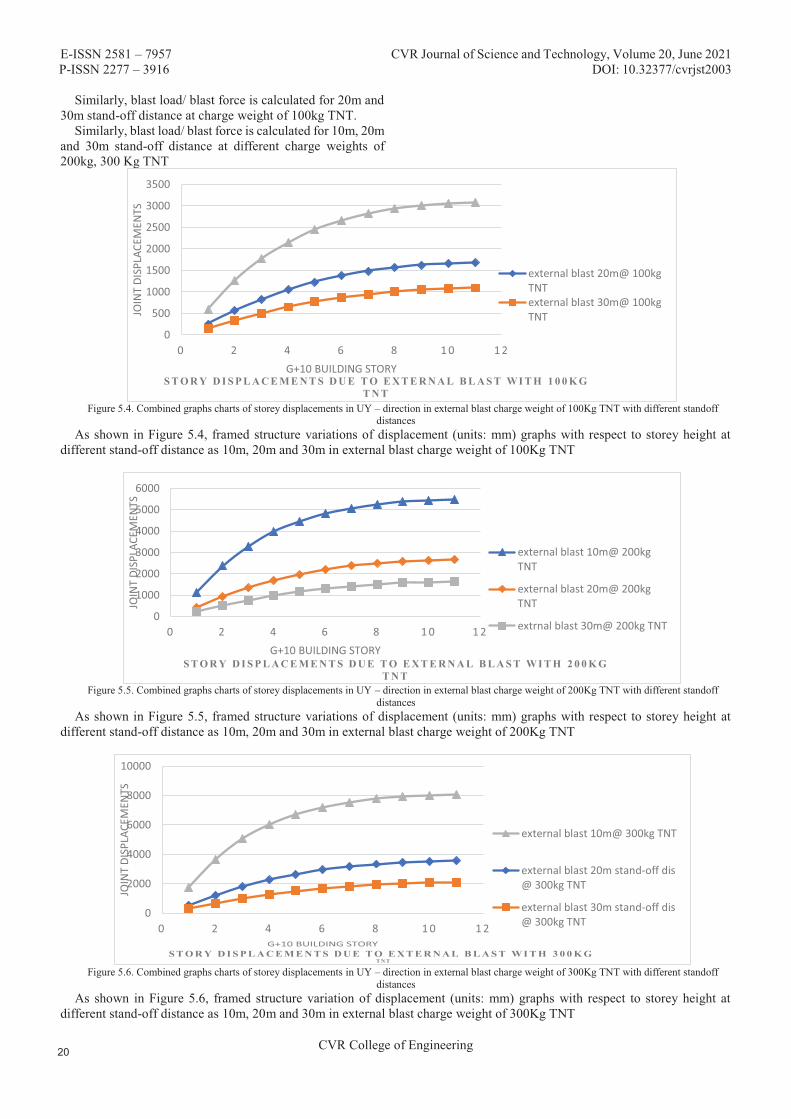
E-ISSN 2581 – 7957 CVR Journal of Science and Technology, Volume 20, June 2021 P-ISSN 2277 – 3916 DOI: 10.32377/cvrjst2003
CVR College of Engineering
Similarly, blast load/ blast force is calculated for 20m and 30m stand-off distance at charge weight of 100kg TNT.
Similarly, blast load/ blast force is calculated for 10m, 20m and 30m stand-off distance at different charge weights of 200kg, 300 Kg TNT
Figure 5.4. Combined graphs charts of storey displacements in UY – direction in external blast charge weight of 100Kg TNT with different standoff
distances As shown in Figure 5.4, framed structure variations of displacement (units: mm) graphs with respect to storey height at
different stand-off distance as 10m, 20m and 30m in external blast charge weight of 100Kg TNT
Figure 5.5. Combined graphs charts of storey displacements in UY – direction in external blast charge weight of 200Kg TNT with different standoff
distances As shown in Figure 5.5, framed structure variations of displacement (units: mm) graphs with respect to storey height at
different stand-off distance as 10m, 20m and 30m in external blast charge weight of 200Kg TNT
distances As shown in Figure 5.6, framed structure variation of displacement (units: mm) graphs with respect to storey height at
different stand-off distance as 10m, 20m and 30m in external blast charge weight of 300Kg TNT
0
500
1000
1500
2000
2500
3000
3500
0 2 4 6 8 1 0 1 2
JOIN
T DI
SPLA
CEM
ENTS
G+10 BUILDING STORYS T O R Y D I S P L A C E M E N T S D U E T O E X T E R N A L B L A S T W I T H 1 0 0 K G
T N T
external blast 20m@ 100kgTNTexternal blast 30m@ 100kgTNT
0
1000
2000
3000
4000
5000
6000
0 2 4 6 8 1 0 1 2
JOIN
T DI
SPLA
CEM
ENTS
G+10 BUILDING STORYS T O R Y D I S P L A C E M E N T S D U E T O E X T E R N A L B L A S T W I T H 2 0 0 K G
T N T
external blast 10m@ 200kgTNT
external blast 20m@ 200kgTNT
extrnal blast 30m@ 200kg TNT
0
2000
4000
6000
8000
10000
0 2 4 6 8 1 0 1 2
JOIN
T DI
SPLA
CEM
ENTS
G+10 BUILDING STORY
T N T
external blast 10m@ 300kg TNT
external blast 20m stand-off dis@ 300kg TNT
external blast 30m stand-off dis@ 300kg TNT
S T O R Y D I S P L A C E M E N T S D U E T O E X T E R N A L B L A S T W I T H 3 0 0 K G
Figure 5.6. Combined graphs charts of storey displacements in UY – direction in external blast charge weight of 300Kg TNT with different standoff

E-ISSN 2581 – 7957 CVR Journal of Science and Technology, Volume 20, June 2021 P-ISSN 2277 – 3916 DOI: 10.32377/cvrjst2003
CVR College of Engineering
G. Shear wall It is a structural system composed of braced panels to
counter the consequences of lateral load appearing on a structure. [11] Section property of shear wall
1. Reinforced Concrete shear wall Thickness-150mmMaterial property of shear wall
1. Material property of shear wall (concrete) M20
Figure 5.7. G+10 storey building with reinforced concrete external shear walls
The blast load with same intensity and standoff distance is applied with respect to beam column joint structure with external concrete shear walls as shown in Fig 5.7 design Rule’s setup in finite element software SAP2000 we get detail Report in displacement and story drift of RCC building.
Similarly blast load is calculated for different charge weights of 100kg, 200kg and 300kg TNT at stand-off distance 10m, 20m and 30m
Figure 5.8. Combined graphs charts of storey displacements in UY – direction with shear walls in external blast charge weight of 100Kg TNT with different standoff distances
As shown in Figure 5.8, framed structure with shear walls variation of displacement (units: mm) graphs with respect to storey height at different stand-off distance as 10m, 20m and 30m in external blast charge weight of 100Kg TNT
0
100
200
300
400
500
600
0 2 4 6 8 10 12
JOIN
T DI
SPLA
CEM
ENTS
G+10 BUILDING STORYS T O R Y D I S P L A C E M E N T S D U E T O E X T E R N A L B L A S T W I T H 1 0 0 K G T N T
external blast with shear walls20m @100kg TNTexternal blast with shear walls30m @100kg TNTLinear (external blast with shearwall 10m @100kg TNT)
E-ISSN 2581 – 7957 CVR Journal of Science and Technology, Volume 20, June 2021 P-ISSN 2277 – 3916 DOI: 10.32377/cvrjst2003
CVR College of Engineering
Figure 5.9. Combined graphs charts of storey displacements in UY – direction with shear walls in external blast charge weight of 200Kg TNT with
different standoff distances As shown in Figure 5.9, framed structure with shear walls variation of displacement (units: mm) graphs with respect to storey
height at different stand-off distance as 10m, 20m and 30m in external blast charge weight of 200Kg TNT
Figure 5.10. Combined graphs charts of storey displacements in UY – direction with shear walls in external blast charge weight of 300Kg TNT with
different standoff distances As shown in Fig. 5.10, framed structure with shear walls variation of displacement (units: mm) graphs with respect to storey
height at different stand-off distance as 10m, 20m and 30m in external blast charge weight of 300Kg TNT
VI. NON – LINEAR DYNAMIC ANALYSIS
Non-linear analysis is an analysis where a nonlinear relation holds between displacement and time. This is opposed to linear static analysis. When a blast force is exposed to structure with respect to time, the change of the output is not proportional to the change of the input. [8]
Time history analysis is used to determine the blast response structure under powerful stacking. Time history investigation is a stage through advance assessment of the dynamic reaction of a structure to a focused-on stacking that may likewise vary with time. [8]
A structure subjected to an external explosion; the fundamental natural period of the structure introductory positive pressure stage followed by a negative stage at any point as shown in Figure 6.1. The impact wave is going through a blast wind causing dynamic pressures. If the period of the positive segment, then it offers with an impulsive loading as shown in Figure 6.2. [8]
Figure 6.1. Triangular pulses and definition of relevant fictitious times
[12]
0
200
400
600
800
1000
1200
0 2 4 6 8 10 12
JOIN
T DI
SPLA
CEM
ENTS
G+10 BUILDING STORYS T O R Y D I S P L A C E M E N T S D U E T O E X T E R N A L B L A S T W I T H 2 0 0 K G T N T
external blast with shear wall20m @ 200kg TNT
external blast with shear wall30m @ 200kg TNT
external blast with shear walls10m @200 kg TNT
0200400600800
10001200140016001800
0 2 4 6 8 10 12
JOIN
T DI
SPLA
CEM
ENTS
G+10 BUILDING STORYS T O R Y D I S P L A C E M E N T S D U E T O E X T E R N A L B L A S T W I T H 3 0 0 K G T N T
external blast with shear walls20m stand-off @300kg TNT
external blast with shear walls30m stand-off @300kg TNT
external blast with shear walls10m @300 kg TNT
E-ISSN 2581 – 7957 CVR Journal of Science and Technology, Volume 20, June 2021 P-ISSN 2277 – 3916 DOI: 10.32377/cvrjst2003
CVR College of Engineering
Figure 6.2. Pressure – Impulse diagram. [12]
A G+10 storey RCC commercial building is subjected to
100kg Trinitrotoluene (TNT) blast source at the central point of the structure at the ground level was considered throughout the external surface of the building, at a stand-off distance 10m.
Figure 6.4. Rare Face graph Pressure and time of Explosion in time
history function
Figure 6.3. Front Face graph Pressure and time of Explosion in time history function

E-ISSN 2581 – 7957 CVR Journal of Science and Technology, Volume 20, June 2021 P-ISSN 2277 – 3916 DOI: 10.32377/cvrjst2003
CVR College of Engineering
Figure 6.5. Time history analysis by non-linearity
A. Output curves – time history function analysis
Figure 6.6. Plot function Displacement vs Time

E-ISSN 2581 – 7957 CVR Journal of Science and Technology, Volume 20, June 2021 P-ISSN 2277 – 3916 DOI: 10.32377/cvrjst2003
CVR College of Engineering
Figure 6.7. Nodal Displacements on the front middle structure vertical
Figure 6.8. Plot function of Acceleration vs Time

E-ISSN 2581 – 7957 CVR Journal of Science and Technology, Volume 20, June 2021 P-ISSN 2277 – 3916 DOI: 10.32377/cvrjst2003
CVR College of Engineering
Figure 6.9. Plot function of Velocity vs Time
Figure 6.10. Plot function of Torsion vs Time
VII. RESULTS AND DISCUSSIONS
� A G+10 RCC structure is subjected to external blast at 10m, 20m, and 30m stand-off distances and charge weight about 100kgs TNT blast load in each case is calculated from IS 4991-1968 by this highest lateral displacement is 3089mm, 1680mm, and 1092mm Similarly, building is designed with shear walls of 150mm thickness external surface of building with same impact structure is subjected to external blast of 100kg TNT at a standoff distances 10m, 20m, and 30m where highest lateral displacement is 534mm, 240mm, and 146mm displacement was decreased about 82%, 85%, and 86%
� Again G+10 RCC structure is subjected to external blast at 10m, 20m, and 30m stand-off distances and charge weight about 200kgs blast load in each case is calculated from IS 4991-1968 by this highest lateral displacement is 5475 mm, 2664mm, and 1627mm Similarly, building is designed with shear walls of 150mm thickness external surface of building with same impact structure is subjected to external blast of 200kg TNT at a standoff distances 10m, 20m, and 30m where highest lateral displacement is 1002mm, 387mm, and 220mm displacement was decreased about 81%, 85%, and 86%
� Again G+10 RCC structure is subjected to external blast at 10m, 20m, and 30m stand-off distances and charge weight about 300kgs blast load in each case is calculated

E-ISSN 2581 – 7957 CVR Journal of Science and Technology, Volume 20, June 2021 P-ISSN 2277 – 3916 DOI: 10.32377/cvrjst2003
CVR College of Engineering
from IS 4991-1968 by this highest lateral displacement is 8080mm, 3549mm, and 2110mm Similarly, building is designed with shear walls of 150mm thickness external surface of building with same impact structure is subjected to external blast of 300kg TNT at a standoff distances 10m, 20m, and 30m where highest lateral displacement is 1541mm, 515mm, and 287mm displacement was decreased about 80%, 85%, and 86%
VIII. CONCLUSIONS
In present study a R.C.C structure was analyzed for blast load in different parametric conditions. When the blast load hits to structure, the blast pressure leads to an increase in the kinetic energy of the structural system. The increase in velocity results in a large displacement of the framed elements.
Variation of displacement is Non-Uniform along the height of building and reached to Collapse Point for minimum standoff distance.
Effects of blast loads can also be decreased by providing lateral moment resisting frames like shear wall
REFERENCES
[1] IS 4991:1968, Criteria for blast resistant design of structures for explosions above ground
[2] Suraj D Bhosale, Shrinivas.R.Survanshi, “Dynamic analysis of RCC frame structure subjected to blast loading without infilled wall in multi storey building”,
International Journal of Current Engineering and Technology, Vol.6, No.3 (June 2016)
[3] P. Srinivasa Rao, P. Manoj Kumar, G. Tirupathi Naidu, “Study the impact of blast load on G+7 multistoried RCC structure with varied distances”, (IJITEE), ISSN: 2278-3075, Volume-8 Issue-4, February 2019
[4] Nitesh N. moon, “Prediction of blast loading and its
impact on buildings”, NIT Rourkela, 2009 [5] Ashish Kumar Tiwari, “Analysis of structural response
under blast loading using sap - 2000 and autodyn”,
Jaypee University of Information and Technology Waknaghat Solan, 2015
[6] M. Meghanadh, T. Reshma, “Blast analysis and blast
resistant design of R.C.C residential building”, (IJCIET) Volume 8, Issue 3, March 2017
[7] Quazi Kashif, Dr. M. B. Varma, “Effect of blast on g+4
RCC frame structure”, IJETAC, ISSN 2250-2459, ISO 9001:2008 Certified Journal, Volume 4, Issue 11, November 2014
[8] Priyanka A., Rajeeva S. V., “Dynamic response of a
multi-story building under blast load”, The International Reviewer Volume 2 Issue 1 January - June 2015 pp. 17-20 ISSN 2395-1575
[9] Thejashwini, Dr. M N Hegde, “Effect of blast loads on
multistoried RCC building”, (IRJET), Volume: 05 Issue: 07 July 2018
[10] A. Lalitha, V. Lakshmi, “Analysis of g+5 RC building
for blast forces”, (IJSR), ISSN: 2319-7064 (2018) [11] Kanchan Pujari, Prof. D.H. Tupe, Prof. Dr. G.R.
Gandhe, “Response of a rectangular reinforced concrete
structure with and without shear walls under blast loadings”, (IRJET), e-ISSN: 2395-0056 Volume: 06 Issue: 05 May 2019
[12] Vasilis KARLOS, George SOLOMOS, “Calculation of blast loads for application to structural components”,
Luxembourg: Publications Office of the European Union, 2013

Abstract: Regular construction practices focus makes use of reinforcing bars for transferring forces. Method of lap Splice is generally used for ensuring continuity of reinforcement steel. However, this method results in minor defects such as joint failure, inadequate length for lapping, improper welding of bars, increased cost of labor etc.
A comparative study of column reinforcement with couplers and without couplers as lap splices was carried out through a case study of an under construction building. Initially the quantity of reinforcing bars required for conventional lap splicing of columns was estimated. The value of steel for providing lap splices within the columns was also determined. Finite element analysis of coupled rebar is carried out to check for the yielding and ultimate stresses developed. These values are verified with that specified in the code. The use of couplers significantly decreases construction time and quantity of steel required in lapping.
The use of couplers as lap splices provides an economic way of connecting reinforcement without adversely affecting the strength of the joint.
Index Terms: Conventional lap spicing, reinforcement couplers, threading, Joints, Columns, FEA.
I. INTRODUCTION

�
�
�
�
II. LITERATURE REVIEW
III. METHODOLOGY

IV. ESTIMATION

Diameter of Bar (mm)
Length of Lap @50d (m)
Length of bars (m)
Weight of bars/Rmt (kg) Total Weight
(kg)
Rate of steel reinforcement/kg
(in Rs)
Total Amount (in Rs)
Diameter of Bar (mm)
No. of Laps
Cost of coupler per unit
(in Rs) Total Amount
For couplers (in Rs) (A)
Minimum thread Length
Price per mm
Cost of threading for one coupler
Total Amount for
Threading(in Rs) (B)
Total Amount (in Rs) for coupler and
threading (A+B)
S.No. Dia of Bar
(mm)
Cost of Lap length
(in Rs)
Cost of Coupler
(in Rs)
Difference (%)
Diameter of Bar (mm)
No. of Columns (A)
No. of Bars (B)
Cost of Lap (C) (in Rs)
Cost of Couplers (D) (in Rs)
Cost of Lapping (A*B*C) (in Rs)
Cost of Couplers (A*B*D) (in Rs)
Difference (%)

Diameter of Bar (mm)
Grade of Rebar
Yield stress (N/mm2)(as per IS 1786-1985)Yield stress Obtained
(N/mm2) Ultimate stress(N/mm2)(as per IS 1786-1985)
Ultimate stressObtained(N/mm2)
V. CONCLUSIONS
REFERENCES

E-ISSN 2581 –7957 CVR Journal of Science and Technology, Volume 20, June 2021P-ISSN 2277 – 3916 DOI: 10.32377/cvrjst2005
CVR College of Engineering
Intelligent Aspect based Model for Efficient Sentiment Analysis of User Reviews
Dr. M. Deva Priya1 and R. Rithika2
1Assoc. Professor, Sri Krishna College of Technology/CSE Department, Coimbatore, Tamil Nadu, IndiaEmail: [email protected]
2UG Scholar, Sri Krishna College of Technology/CSE Department, Coimbatore, Tamil Nadu, IndiaEmail: [email protected]
Abstract: Mining online reviews to extract opinion targets and words are substantial tasks in fine-grained opinion mining. The main aim is to mine sensible multi-grain aspects and opinion words from unlabeled reviews. In this paper, Combined Aspect based Sentiment Model (CASM) is propounded to cooperatively mine multi-grain features and opinions. CASM deals with aspects, opinions, sentiment polarity and granularity concurrently. Support Vector Machine-Radial Basis Function kernel (SVM-RBF) classifier is applied to improve CASM by splitting aspects and opinion words. CASM-SVM-RBF deals with two different kinds of aspects and opinions: general and particular aspects, overallopinions and aspect-precise opinions. Candidates with improved confidence are mined as opinion targets or words.The performance is analyzed in terms of Accuracy, Precision, Recall and F-Score for KNN, BPNN, NBC and ME classifiers.
Index Terms: Aspects, Opinions, Sentiments, Support Vector Machine, Radial Basis Function, Support Vector Machine (SVM), Radial Basis Function (RBF)
I. INTRODUCTION
In recent times, many online shopping sites have come into existence with the speedy increase of e-commerce and online merchants. To provide customer satisfaction, merchants and producers call for customer reviews that include views of the products bought or services demanded.Finally, the customers’ opinions on the numerous aspects of entities are aggregated. The aspects of different granularities are to be automatically extracted, followed by identification of related opinions, particularly aspect-basedopinions and classification of sentiment polarity.
These reviews subsequently become an intellectual basisof information. This information base is beneficial tocustomers and producers. Based on the reviews, the customers take decisions whether to buy a product or not.The producer on the other hand uses this information to comprehend and know the likings of customers. It greatlyaids them in developing better products, marketing and maintaining consumer relationship. Further, these customer reviews inspire the decisions of other customers. Hence, these reviews play a dominant role in supporting the business organizations to implement their development plans. There are 2 categories of textual data namely, facts and opinions. Web searching and text mining deal with facts. Opinion mining encompasses Natural Language Processing (NLP), computational linguistics and text mining. It involves study of emotions, sentiments and opinions conveyed in text.
A sentiment is a thought, view or attitude that is based on emotion. Opinion mining is otherwise called sentiment analysis. This field is used by organizations or individuals for knowing the overall sentiment related to a specific objectlike product, person, movie, institution etc., Earlier, with insufficient admittance to user produced opinions, research in this field was insignificant. With the incredible growth of the World Wide Web (WWW), vast amounts of texts including blogs, reviews, etc., have become available for analysis. WWW is the quickest, wide-ranging and effortlessly available medium that supports sentiment analysis.
Nevertheless, finding opinions and observing them on the web is a challenging task as varied sources are availablewith enormous amount of information. From a human’s viewpoint, it is demanding and tedious to find suitablesources, mine relevant sentences, read and process them,and establish them into a serviceable form. Here comes the need for an automated mining and summarizing model.Various models are available in the literature that process some of these tasks, but little work is done in developing models that enable all the operations to be performed concurrently.
In this paper, a Combined Aspect based Sentiment Model (CASM) model is proposed to cooperatively extract multi-grain aspects and opinions that is capable of addressing all the tasks. CASM is capable of dealing with the aspects,opinions, sentiment polarity and granularity concurrently.To perform separation of opinion and aspect words, CASM-SVM-RBF is proposed, wherein Support Vector Machine-Radial Basis Function kernel (SVM-RBF) classifier is applied to improve CASM.
A. Opinion MiningOpinion mining is a version of Natural Language
Processing (NLP) which is extensively used to track a particular product that the customer is opting. It is also known as sentimental analysis and acts as a platform that builds a system to categorize opinions over a product.Opinion mining can be integrated with Machine Learning (ML) to automate the process, thus forming a system for analyzing sentiments. It helps marketers to:
� Analyze the reach and success of an advertisement/ launch of a product
� Regulate a product/service’s versions� Assess the statistics of pros/cons of a particular
product

E-ISSN 2581 –7957 CVR Journal of Science and Technology, Volume 20, June 2021P-ISSN 2277 – 3916 DOI: 10.32377/cvrjst2005
CVR College of Engineering
For example, a mobile phone may have positive feedbacks considering the camera quality, yet might contain negatives reviews relating to the weight of the phone. This facilitates the vendor to obtain a clear idea of public opinion in contrast to the focus groups or surveys, as the reviews rendered thus are from customers.
Levels of Opinion Mining Opinion mining tasks are categorized based on the level
at which mining is performed. The different levels include: � The document level� The sentence level � The feature level
� Document level - Documents are categorized based on sentiments into positive, negative and neutral polarity. It is assumed that the document focuses only on a single aspect of the object. Opinions from the opinion holder are also included.
� Sentence level - At this level, data is classified into objective, subjective or opinionated text from the corpus and subjective or opinionated sentences are identified. As a result, the sentences in the document are classified into positive, negative and neutral polarities.
� Feature level - There are a number of tasks involved in this level which are listed below: � Task 1: It recognizes and extracts object features
commented on review/text� Task 2: Deals with inferring the opinions as
positive, negative or neutral� Task 3: Groups similar features and produces
feature based opinion summary of multiple reviews/text
These tasks are performed if the features and the synonyms are unknown. If the features are known, and the synonyms are unknown, then all the tasks are to be performed though the third step is easier. The new features that are discovered are mapped with the existing features. If they match, it is mandatory to perform task 2.
B. Challenges in Opinion MiningFollowing are some of the challenges of opinion mining:� A word can sound positive and negative in various
circumstances. The words render completely different meanings in each of the scenarios. For instance, with respect to a product review of a mobile, the word “long” gives a positive outlook when it is described for battery performance but gives a negative opinion when it comes to the booting speed. Therefore, the proposed system must be able to identify the category of opinions.
� It is to be noticed that the choice of expression varies for a large span of people. Small changes between two text fragments do not hinder the contextual meaning. But, as far as opinion mining is concerned, basic conjunctions like ‘and’, ’but’ and words that offer remarks like ‘not’ and ‘very’ must be scrutinized.
� Some views might be contradictory in the sense, the reviews can include both positive and negative statements which can be best suited for analysis when each sentence is analyzed separately. Due to the informal medium that is addressed, the reviews are complex with a variety of opinions in a single sentence. Like the remark which states “The overall performance is very good except for the longevity of the battery charge which is not encouraged.”
C. Sentence-Level Sentiment Analysis Web opinion mining revolves around sentimental
classification at the document-level. Document-level classification being too coarse for a majority of the applications, analysis is applied at the sentence-level. Classifying sentences based on objective or subjective speech is the main agenda of this analysis, and not extracting subjective sentences in news articles.
II. RELATED WORK
Opinion target and word extraction are the predominant tasks involved in opinion mining. Much work is done on them [1-5]. Opinion mining is divided into two types:sentence-level and corpus level based on their extraction aims. Hu & Liu (2004) [1] have used nearest-neighbor rules to recognize opinion relations that exist among words. Using a bootstrapping process, frequent and explicit product features are extracted. Using co-occurrence information or nearest-neighbor rules can never help in precisely detecting opinion relations among words.
Popescu & Etzioni (2007) [4] have used syntax related information to mine opinion targets and have developed syntactic patterns that identify opinion associations amid words. They have shown that their scheme is better than that of Hu & Liu (2004) [1, 6]. Identifying and computing opinion associations among words are the key components. Wang & Wang (2008) [5] have used the co-occurrence frequency of opinion targets and words to specify associations.
In Sequence-labelling problems, extraction at sentence-level deals with extracting opinion targets or words by identifying the opinion targets or expressions [7-9].Naturally, appropriate words are considered as features that specify opinion targets/words in sentences.
Ma & Wan et al (2010) [9] have also used CRF to mine opinion targets from reviews. These methods make use oflabelled data for model training. In case of insufficientlabelled training data, data is taken from varied domains in contrast to the available text leading to reduction of the extraction performance. They have propounded a mechanism that depends on transfer learning to ease cross domain mining of opinion targets/words. This mechanismuses labelled data from out-domains as the miningperformance wholly depends on the significance of in-domain and out-domain. Further, more work is done on corpus-level mining. Opinion target/word in sentences is not identified, but a set of opinion targets is mined or a sentiment word lexicon is generated from texts. Much of the earlier schemes have used a cooperative unsupervised mining framework.
E-ISSN 2581 –7957 CVR Journal of Science and Technology, Volume 20, June 2021P-ISSN 2277 – 3916 DOI: 10.32377/cvrjst2005
CVR College of Engineering
Further, traditional sequence labelling models such as Conditional Random Fields (CRFs) [10] and Hidden Markov Model (HMM) [11] are also used for extraction. Jin et al (2009) [11] have propounded a lexicalized HMM model to perform opinion mining.
Various authors have used topic modelling to detect inherent topics and sentiment words [12-15]. The main goal is not to mine an opinion target or word lexicon, but cluster words into conforming features in reviews. These mechanisms have used frequency statistics and phrase identification to identify right opinion targets/words. They have emphasized on clustering words into consistent topics or features. Mining opinion targets and words from online reviews are significant tasks in opinion mining, which involve identifying opinion associations among words.
Qiu et al (2009) [16] & Qiu et al (2011) [17] have propounded Double Propagation that involves syntactic associations amongst words to iteratively enlarge sentiment words and opinion targets. The chief restriction is that the patterns are based on dependence parsing tree and hence do not deal with all opinion associations. Liu et al (2012) [18]have dealt with opinion target mining based on unsupervised WAM that captures opinion associations in sentences. Opinion targets are mined in a regular random walk framework making it efficient for mining opinion targets. However, they have not dealt with demonstrating the efficiency of the WAMon opinion word mining. Kaur & Gupta (2013) [19] have stated that the machine must be able to infer the NLP techniques well before sentimental analysis phase. This technique is tested against languages like English, Hindi with the help of senti-wordnet to estimate the polarity of the sentences. To accomplish this, the machine is required to fathom NLP through training. Hasan et al (2014) [20] have performed sentimental analysis with Bangla text. In spite of acquiring senti-wordnet, the experiment displays difficulty in analysis as the texts are completely in Bangla and not English.
Asghar & Khan (2014) [21] have proposed a sentimental analysis which classifies subjective and objective sentences from collection of reviews. They have used senti-wordnet to predict the score by determining the polarity of the sentence.Ahmed et al (2015) [22] have surveyed on tool enhancement methods and tools available for analysis. Though the analysis of the applications is done, the comparative approaches for these applications are not accomplished. Sri & Ajitha (2016) [23] have applied sentiment classification to conduct a survey on product reviews. Frequent terms are found easily by using a new technique named semantic orientation. With time complexity and accuracy as parameters, a comparative study between existing and proposed solutions is conducted which shows that semantic orientation is the best.
Zhang et al (2017) [24] have stated that opinions rendered on various aspects of entities described in larger scale online reviews require automatic extraction of granularities, recognizing opinions that associate with the granularity and categorizing sentiments based on polarity. Although various models are proposed to process few of the tasks, a model to simultaneously perform the task is uncommon. This model focuses on separating polarity, opinion and model aspects
separately. To do so, Joint Aspect-Based Sentiment Topic with Maximum Entropy (JABST-ME) classifier is applied. Dubey et al (2018) [25] have suggested an item based collaborative filtering system to overcome the demerits of the conventional collaborative algorithm. The authors have proposed an improved recommender system. The system involves a record of sentiment scores which is determined by calculating the positive reviews. The scores are thus used in a filtering system which differentiates the overall negative user opinions from positive ones so as to improve the recommendation of the product.
Al-Ayyoub et al (2019) [26] have dealt with the online social networks that have paved the way for many domains including analysis of networks and contents to derive information. Sentimental analysis being one of the advancement is involved in extracting sentiments conveyed in the content. Though sentimental analysis has its own history, it has been in use from the recent decade as this allows users to interact over the network and post their views and opinions. Gopi et al (2020) [27] have conducted a survey from which it is inferred that some of the social networking platforms like Facebook offer users an option to express their opinions through emojis. Classifying opinions into different categories is termed as opinion mining,whereas defining a score for these opinions falls under sentimental analysis. The opinions are scored with numbers ranging from -5 to 25. To prove the theory, movie review data from twitter from the years 2013 to 2020 is used.Sankar et al (2020) [28] have proposed a technique for sentiment classification. To obtain optimal words, Machine Learning (ML) based techniques offer better results. The resulted features are then fed into a Neural Network (NN) for further processing. The approach is evaluated for the datasets like rotten tomatoes. This system is tested over an android application framework on smart phone reviews without the aid of cloud or server side Application Programming Interface (API) to offer effective results.
III. TEXT CLASSIFICATION MECHANISMS
In this section, some of the renowned text classificationschemes are discussed.
A. K-Nearest Neighbor (KNN) AlgorithmK-Nearest Neighbor (KNN) is simple to understand and
implement. It is based on statistics and not parameters. It makes decisions based on the trained data. KNN guesses whether the data is present in a feature space or not. Gene array vector is taken as input. Similarity measurement using different measures such as Euclidean, Minkowski and Manhattan are computed and the KNN classifier is trained using the selected features.
KNN depends on a distance function for pairs of data samples such as the Euclidean distance and Pearson’s correlation of their gene expression profiles. The data samples are classified based on the class memberships of their ‘K’ nearest neighbors. Many researchers prefer KNN due to its simplicity and its better performance. The classifier defines non-linear decision limits i.e. KNN improves the performance when the sample has insignificant non-linear variations around the decision margin result.

E-ISSN 2581 –7957 CVR Journal of Science and Technology, Volume 20, June 2021P-ISSN 2277 – 3916 DOI: 10.32377/cvrjst2005
CVR College of Engineering
Given an input gene array vector, the classifier extracts the reference set of ‘K’ nearest vectors based on the similarity and decides the label of input vector based on the classifier. Pearson’s coefficient correlation, Euclidean, Manhattan and Minkowski distances represent the similarity measures. For an input ‘x’ and a reference set,
(1)
The probability that ‘x’ can fit into a class is given by:
(2)
where,- Similarity amid ‘x’ and ‘ ’
- Bias term
B. Back-Propagation Neural Networks (BPNN)Back-Propagation Neural Networks (BPNN) is generally
used in training Deep Neural Networks (DNNs) to evaluate the error influence of each neuron for a set of data that is handled [29]. It is an unusual case of automatic differentiation. It is commonly used in adjusting the neuron weights by finding the gradient loss function. This mechanism is also known as backward propagation of errors, as the errors are computed in the output layer and sent back. It demands a known, preferred output for every input and is considered as a supervised learning method.
Back-Propagation is the essence of neural net training. It is the act of streamlining the weights of a neural net with the help of error rate acquired in the former iteration. Appropriate tuning of the weights guarantees lesser error rates making the model dependable by expanding its speculation. The algorithm searches for the reduced value of error function in the weight space by utilizing an approach known as the delta rule or gradient descent. The weights which limit the error function are considered as solutions for the learning problem.
BPNN is capable of creating complex decision boundaries/limits in the feature space. Even an attempt has been made using Multi-Layer Perceptron (MLP) networks trained with backpropagation, Radial Basis Function (RBF) networks and high-order polynomial networks which strongly recommend that a BPNN under suitable conditions can estimate Bayesian posterior probabilities at its outputs. This is critical on the grounds that a Bayesian classifier gives the finest performance with reduced error rate for a feature data distribution. It is not possible to predict the performance of BPNN similar to other non-parametric ways.Furthermore, some parameters like number of training samples and hidden nodes, and the learning rate are to be chosen.
C. Naïve Bayesian Classifier (NBC)Naïve Bayes Classifier (NBC) is the most common
classifier for text arrangement. It also serves as the basic criteria for redefining a classifier. For instance, an apple is associated with its features, that is, its color and shape. Based on the likelihood of these organic products, the classifiers are able to differentiate products based on theshading in their color, width and roundness. A
demonstration of contingent likelihood is made using a vector d=( ,…..,d), with the probability of p( | ,…..,d) for ‘k’ conceivable classes or results ‘ ’. The classifier defined as,
(3)
where,
D. Maximum Entropy (ME)The Maximum Entropy (ME) belongs to the class of
exponential models as it is a probabilistic classifier. ME unlike Naive Bayes Classifier (NBC) does not limit the repetition of the highlights. The MaxEnt function based on the principle of ME focuses on choosing the model withhigh entropy values from a pool of models that match the prepared information. The content order issues can besegregated under various aspects using ME classifier. A few issues which may occur frequently include point characterization, dialect location and supposition examination.
The parameters of a chosen model have to be assessed prior to further execution for which, ME requires a considerable amount of time to prepare and process the underlying goal, while NBC does not.
The first step is to look into the following arrangement ( , ) wherein ‘ ’ stands for the logical data corresponding to the record (meagre cluster) and ‘ ’ is it’s respective class. The second step focuses on outlining the preparation test approximating to its exact likelihood:
(4)Where,m - Size of the training datan -
The indicator function is given by,
(5)
The probability of class is derived as:(6)
Where,d - Class of the modele - Data point
- Weight vector.
ME poses to be much efficient with respect to NBC over the following reasons:
� Accurate classification in contrast to NBC� Portrays consistency and sign of improvement� Proves to be efficient when dealing with a large
volume of data� Easy processing of data irrespective of the
differences in formats

E-ISSN 2581 –7957 CVR Journal of Science and Technology, Volume 20, June 2021P-ISSN 2277 – 3916 DOI: 10.32377/cvrjst2005
CVR College of Engineering
E. Support Vector Machine (SVM)Support Vector Machine (SVM) [30] is a widely used
classifier. They are particularly helpful for predicting numerical data, classification and pattern matching techniques. They consider boundaries between data points, focusing on the decision boundary that isolates the data points into classes (or is the most generalizable). The main aim is to have the decision boundary between the points as extensive as possible. This expands the distance between data point and the boundary line.
It is a supervised training model related to learning algorithms for analyzing data and recognizing data patterns. The choice of kernel parameters involved in the training process has an influence on the classification accuracy. Feature selection also plays a major role in classification. It is used in pattern recognition [31], bioinformatics [32] and text categorization [33]. SVM categorizes data by finding a collection of support vectors that belong to a class of training inputs that define a hyperplane in the feature space. It focusses on fitting the hyperplane to the training data by using a kernel function. These functions can be chosen during training to identify support vectors along the functionlimits.
SVM includes kernels like the linear kernel, polynomial kernel and the RBF kernel, out of which the RBF kernel is the most popular. A function ‘y’ that maps a single vector to a higher dimensional vector, approximating the kernel isgiven below.
(7)
Where, ‘Ψ’is the implicit mapping embedded in RBF kernel.
The general function of SVM classifier is given by,
(8)
Where, the feature vector is defined as,
(9)
where, - Free parameter
IV. PROPOSED SYSTEM
In the present system, the opinions are categorized intopositive and negative types. Those with neutral opinions are not categorized precisely. Sentiment scores are computed using Senti-WordNet or WordNet tools which includescoring functions to measure the positive/ negative scoresproficiently when compared to the neutral score. The proposed system capable of dealing with neutral opinions and a scoring function is designed to offer a better scoring.The proposed system includes the following phases namely, data extraction, opinion extraction and sentiment evaluation.
An aspect term called feature indicates a particularattribute or component of an entity (product) which is anoun or noun phrase. For example, “voice” is an aspect in areview related to audio CD review. To accumulate opinions on features of objects in online reviews, it is significant to mine aspects of diverse granularities, recognize relatedopinions, particularly aspect-specific opinions and computesentiment polarities. The propounded mechanism includes the ensuing steps. In the text mining stage, stop words and symbols are removed. Feature extraction is carried out using stemming, finding Term Frequency (TF) and using Bag of Words (BoW) (Figure 1).
A. Data CollectionData is collected from user reviews in blogs, forums and
social networks that are not structured properly. It may be conveyed in diverse ways including various words, vernaculars and framework, thus making human analysis complex. Text analytics and NLP ease the process of extraction and classification.
B. Pre-processingIn this phase, the data is pre-processed to eliminate noise
and reduce dimensions. Verbs, nouns and non-verbs in the sentences are identified. The non-textual and inappropriate details are removed from the mined data. For example: common words like “computer” and “touchpad” are identified as aspects. To be specific, “computer” is recognized as a common aspect, while “touchpad” is identified as a particular aspect. It involves the following steps - Tokenization, Stop Word Removal, Stemming, Term Frequency-Inverse Document Frequency (TF-IDF) based feature extraction.
E-ISSN 2581 –7957 CVR Journal of Science and Technology, Volume 20, June 2021P-ISSN 2277 – 3916 DOI: 10.32377/cvrjst2005
CVR College of Engineering
Figure 1. Proposed System
TokenizationTokenization deals with splitting strings into tokens
which include words, keywords, phrases, symbols etc., Symbols like punctuation marks are cast-off and meaningful keywords are recognized. In short, it is the process of delineating and categorizing sections of a string. The words in a sentence are explored and consistency is established.
Stop Word RemovalStop words include the most frequently used words like
‘a, the, an, in’. The search engine ignores them while searching and extracting them based on the query. Removing them reduces the processing time. Stop words are removed before processing of text in natural language. Themost common stop words that support text mining areprepositions, articles and pro-nouns.
StemmingStemming is the process of condensing a word to its word
stem that relates to the prefix, the suffix or the root word known as lemma. It is also a pivotal component in Natural Language Understanding (NLU) and NLP. Stemming coupled with AI is extensively used for information extraction from big data sources. Interestingly enough, they also serve as a part of the search engine querry for quicker retrieval of data.
Term Frequency-Inverse Document Frequency (TF-IDF)based Feature Extraction
In this phase, the information with worthy reviews is
considered. It is the product of the frequencies of the word considered (TF) and the word in whole corpus
(IDF) [34].
(10)
- Weight of a term ‘i’ - Frequency of term ‘i’ in sample ‘j’
N - Number of samples in the corpus
- Number of samples with ‘i’
Adaptive words like ‘good’, ‘bad’, ‘very’, ‘not’, and conjunctions like ‘and, ‘but’ are identified. Adjectives are to be identified so that the product can be rated correctly. The customers would have rated one aspect positively, but another negatively. The ratings of both the features are to betaken into account while deciding the quality of the product.Combined Aspect based Sentiment Model (CASM) model is propounded to cooperatively mine multi-grain aspects and opinions which focus on all the tasks. CASM is capable of dealing with feature, opinion, sentiment polarity and granularity concurrently.
To isolate opinion and aspects, Combined Aspect based Sentiment Model with Support Vector Machine-Radial Basis Function kernel (CASM-SVM-RBF) is proposed, in which SVM-RBF classifier is applied to improve CASM.SVM-RBF classifier is applied to isolate aspect and opinion words. The goal is to mine multi-grain aspect and opinion words from unlabeled reviews. CASM-SVM-RBF is capable of dealing with different types of aspects and opinions like common and specific aspects, common and aspect-precise opinions.
C. SVM-RBF ClassificationThe adjoining words in the user reviews are taken into
account and the aspects are classified into either ‘Positive’ or ‘Negative’. In the proposed scheme, SVM-RBF is used for classification. It is seen that SVM-RBF does effective classification in contrast to KNN, BPNN, NBC and ME classifiers respectively.
D. WordNetWordNet is a huge lexical database of English. Various
viewpoints of a word including nouns, adjectives and adverbs and verbs are collected as cognitive synonyms (synsets), where each has its own structure. To compute the scores of reviews, the dictionary is loaded. By associatingthe reviews with the dictionary, the scores are anticipated.By involving Senti-WordNet, polarity can be computed.Table 1 shows the opinions and polarities.

E-ISSN 2581 –7957 CVR Journal of Science and Technology, Volume 20, June 2021P-ISSN 2277 – 3916 DOI: 10.32377/cvrjst2005
CVR College of Engineering
TABLE I.CLASSIFYING OPINIONS AND POLARITY
Aspect Opinion PolarityMobile screen Big Positive
Battery Not lasting PositiveGenerator More noise Negative
A model is built using SVM-RBF and precision is expected. The scores of the reviews are to be considered.The scores are taken as 1 for positive, -1 for negative and 0 for neutral reviews. Nevertheless, a review can include 2 or more sentiments. To predict the scores, a WordNet vocabulary dictionary which includes positive and negative words is stacked. The sentiment reviews which are cast-offin a record are stacked. By differentiating the reviews and the vocabulary word reference, reviews carrying positive and negative views are efficiently observed and scoring is carried out. Positive and negative reviews along with neutral reviews are considered. A scale of -2 to +2 limit is
considered to envisage the score, where the scale
signifies the values shown in Table 2.
TABLE II.
SCALE FOR SCORES Score Prediction
-2 Awful-1 Poor0 Fair1 Good2 Excellent
V. IMPLEMENTATION
The performance of the model is evaluated for reviews related to electronic devices and restaurants, both qualitatively and quantitatively. It is seen that the proposed model outperforms all the benchmarked schemes taken into consideration. The proposed CASM-SVM-RBF offers better accuracy and involves less time period in contrast to the existing methods and algorithms. The screenshots show the steps involved in classifying user reviews (Figure 2 to Figure 8).
Figure 2. Homepage
Figure 3. Register and log in form
Figure 4. Mining Reviews
Figure 5. Customer Review Selection
Figure 6. Customer Reviews Search Results

E-ISSN 2581 –7957 CVR Journal of Science and Technology, Volume 20, June 2021P-ISSN 2277 – 3916 DOI: 10.32377/cvrjst2005
CVR College of Engineering
Figure 7. Customer Reviews Search Results Positive & Negative Ranges
Figure 8. Product based Positive & Negative Values Calculation
VI. RESULTS AND DISCUSSION
A total of 1892 sentences are taken, and spam and recurrent views shown as emotions are removed. SVM-RBF classifier is used and polarity is computed. Once opinion ismined, around 202 sentences are found unique. UsingWordNet, scores are found.
The analysis involves sentence based sentiment classification. Hence, a lexicon containing positive and negative words is prepared. The neutral scores are alsounderstood. The lexicon dictionary is improved to computethe score for neutral sentences also. The grades are in the range - 2 to +2. The performance is measured in terms of Accuracy, Precision Recall and F-score.
Accuracy: It is the percentage of predictions that are estimated correctly during the process of opinion mining. It is the ratio of number of predictions that confirm the existence of opinions to the number of predictions imposed for detecting opinions derived from the twitter dataset.
(11)
where,TN - Correct predictions of an occurrence as negativeFN - Incorrect predictions of an occurrence as positiveFP - Incorrect predictions of an occurrence as negativeTP - Correct predictions of an occurrence as positive
Precision: It is the percentage of reviews from which opinion is accurately classified. It is the ratio of the
number of opinions detected correctly to the number of reviews considered in the opinion mining process.
(12)
Recall: It is the percentage of opinion mining that ispredicted correctly during the process of opinion mining.
(13)
F-score: It is the weighted average computed between the factor of precision and recall values determined during the process of opinion mining.
(14)
(15)
From Figure 9, it is evident that the SVM_RBF offers 31%, 21%, 16% and 5% better accuracy in contrast to KNN, BPNN, NBC and ME classifiers respectively.
Figure 9. Accuracy
From Figure 10, it is clear that SVM_RBF offers 28%, 22%, 18% and 4% better Precision in contrast to KNN, BPNN, NBC and ME classifiers respectively.
Figure 10. Precision
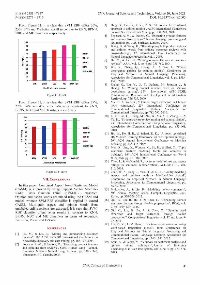
E-ISSN 2581 –7957 CVR Journal of Science and Technology, Volume 20, June 2021P-ISSN 2277 – 3916 DOI: 10.32377/cvrjst2005
CVR College of Engineering
From Figure 11, it is clear that SVM_RBF offers 30%, 23%, 17% and 3% better Recall in contrast to KNN, BPNN, NBC and ME classifiers respectively.
Figure 11. Recall
From Figure 12, it is clear that SVM_RBF offers 29%, 27%, 14% and 4% better F-Score in contrast to KNN, BPNN, NBC and ME classifiers respectively.
Figure 12. F-Score
VII. CONCLUSIONS
In this paper, Combined Aspect based Sentiment Model (CASM) is improved by using Support Vector Machine-Radial Basis Function kernel (SVM-RBF) classifier. Opinion and aspect words are mined using the CASM andmodel, wherein SVM-RBF classifier is applied to extend CASM. Multi-grain aspect and opinion words from unlabeled online reviews are extracted. It is seen that SVM-RBF classifier offers better results in contrast to KNN, BPNN, NBC and ME classifiers in terms of Accuracy, Precision, Recall and F-Score.
REFERENCES
[1] Hu, M., & Liu, B., “Mining and summarizing customerreviews”, 10th ACM SIGKDD International Conference on Knowledge discovery and data mining, pp. 168-177, 2004.
[2] Popescu, A.-M., & Etzioni, O., “Extracting product featuresand opinions from reviews”, Conf. Human Lang. Technol. Empirical Methods Natural Lang. Process., pp. 339 - 346, Vancouver, BC, Canada, 2005.
[3] Ding, X., Liu, B., & Yu, P. S., “A holistic lexicon-based approach to opinion mining”, ACM International Conferenceon Web Search and Data Mining, pp. 231-240, 2008.
[4] Popescu, A. M., & Etzioni, O., “Extracting product featuresand opinions from reviews”, Natural language processing and text mining, pp. 9-28, Springer, London, 2007.
[5] Wang, B., & Wang, H., “Bootstrapping both product features and opinion words from chinese customer reviews with cross-inducing”, 3rd International Joint Conference on Natural Language Processing, vol. I, 2008.
[6] Hu, M., & Liu, B., “Mining opinion features in customerreviews”, AAAI, vol. 4, no. 4, pp. 755-760, 2004.
[7] Wu, Y., Zhang, Q., Huang, X., & Wu, L., “Phrasedependency parsing for opinion mining”, Conference on Empirical Methods in Natural Language Processing, Association for Computational Linguistics, vol. 3, pp. 1533-1541, 2009.
[8] Zhang, Q., Wu, Y., Li, T., Ogihara, M., Johnson, J., & Huang, X., “Mining product reviews based on shallow dependency parsing”, 32nd International ACM SIGIR Conference on Research and Development in Information Retrieval, pp. 726-727, 2009.
[9] Ma, T., & Wan, X., “Opinion target extraction in Chinese news comments”, 23rd International Conference on Computational Linguistics: Posters, Association for Computational Linguistics, pp. 782-790, 2010.
[10] Li, F., Han, C., Huang, M., Zhu, X., Xia, Y. J., Zhang, S., & Yu, H., “Structure-aware review mining and summarization”,23rd International Conference on Computational Linguistics, Association for Computational Linguistics, pp. 653-661, 2010.
[11] Jin, W., Ho, H. H., & Srihari, R. K., “A novel lexicalizedHMM-based learning framework for web opinion mining”,26th ACM Annual International Conference on Machine Learning, pp. 465-472, 2009.
[12] Mei, Q., Ling, X., Wondra, M., Su, H., & Zhai, C., “Topicsentiment mixture: modeling facets and opinions in weblogs”, 16th ACM International Conference on World Wide Web, pp. 171-180, 2007.
[13] Titov, I., & McDonald, R., “A joint model of text and aspectratings for sentiment summarization”, ACL-08: HLT, 308-316, 2008.
[14] Zhao, W. X., Jiang, J., Yan, H., & Li, X., “Jointly modelingaspects and opinions with a MaxEnt-LDA hybrid”,Conference on Empirical Methods in Natural Language Processing, Association for Computational Linguistics, pp. 56-65, 2010.
[15] Mukherjee, A., & Liu, B., “Modeling review comments”,50th Annual Meeting Assoc. Comput. Linguistics, Jeju, Korea, pp. 320-329, 2012.
[16] Qiu, G., Liu, B., Bu, J., & Chen, C., “Expanding domainsentiment lexicon through double propagation”, IJCAI, vol. 9, pp. 1199-1204, 2009.
[17] Qiu, G., Liu, B., Bu, J., & Chen, C., “Opinion wordexpansion and target extraction through double propagation”, Computational linguistics, vol. 37, no. 1, pp. 9-27, 2011.
[18] Liu, K., Xu, L., & Zhao, J., “Opinion target extraction usingword-based translation model”, Joint Conference onEmpirical Methods in Natural Language Processing and Computational Natural Language Learning, Association for Computational Linguistics, pp. 1346-1356, 2012.
[19] Kaur, A., & Gupta, V., “A survey on sentiment analysis andopinion mining techniques”, Journal of Emerging Technologies in Web Intelligence, vol. 5, no. 4, pp. 367-371, 2013.

E-ISSN 2581 –7957 CVR Journal of Science and Technology, Volume 20, June 2021P-ISSN 2277 – 3916 DOI: 10.32377/cvrjst2005
CVR College of Engineering
[20] Hasan, K. A., & Rahman, M., “Sentiment detection from bangla text using contextual valency analysis”, 17th IEEE International Conference on Computer and Information Technology, pp. 292-295, 2014.
[21] Asghar, M. Z., & Khan, A., “Sentiment classification through semantic orientation using SentiWordNet”, Life Science Journal, vol. 11, no. 10, 2014.
[22] Ahmed, K., El Tazi, N., & Hossny, A. H., “Sentiment analysis over social networks: an overview”, IEEE International Conference on Systems, Man, and Cybernetics, pp. 2174-2179, 2015.
[23] Sri, R. J., & Ajitha, P., “Survey of product reviews using sentiment analysis”, International Journal of Science and Technology, 2016.
[24] Zhang, Y., Tang, F., Barolli, L., Yang, Y., & Xu, W., “Jointly modeling multi-grain aspects and opinions for large-scale online review”, 31st IEEE International Conference on Advanced Information Networking and Applications, pp. 570-577, 2017.
[25] Dubey, A., Gupta, A., Raturi, N., & Saxena, P., “Item-BasedCollaborative Filtering Using Sentiment Analysis of User Reviews”, International Conference on Application of Computing and Communication Technologies, pp. 77-87, Springer, Singapore, 2018.
[26] Al-Ayyoub, M., Khamaiseh, A. A., Jararweh, Y., & Al-Kabi, M. N., “A comprehensive survey of arabic sentiment analysis”, Information processing & management, vol. 56, no. 2, pp. 320-342, 2019.
[27] Gopi, A. P., Jyothi, R. N. S., Narayana, V. L., & Sandeep, K. S., “Classification of tweets data based on polarity using improved RBF kernel of SVM”, International Journal of Information Technology, pp. 1-16, 2020.
[28] Sankar, H., Subramaniyaswamy, V., Vijayakumar, V., Arun Kumar, S., Logesh, R., & Umamakeswari, A. J. S. P., “Intelligent sentiment analysis approach using edge computing-based deep learning technique”, Software: Practice and Experience, vol. 50, no. 5, pp. 645-657, 2020.
[29] Nielsen, M. A., “Neural networks and deep learning”, vol. 2018, San Francisco, CA: Determination press, 2015.
[30] Cortes, C., & Vapnik, V., “Support-vector networks”, Machine learning, vol. 20, no. 3, pp. 273-297, 1995.
[31] Pontil, M., & Verri, A., “Support vector machines for 3D object recognition”, IEEE Transactions on Pattern Analysis and Machine Intelligence, vol. 20, no. 6, pp. 637-646, 1998.
[32] Yu, G.X., Ostrouchov, G., Geist, A., & Samatova, N.F., “An SVM-based algorithm for identification of photosynthesis-specific genome features”, IEEE Bioinformatics Conference, pp. 235-243, 2003.
[33] Joachims, T., “Text categorization with support vector machines: Learning with many relevant features”, Springer Berlin Heidelberg, pp. 137-142, 1998.
[34] Mouthami, K., Devi, K.N. and Bhaskaran, V.M., “Sentiment analysis and classification based on textual reviews”, International Conference on Information Communication and Embedded Systems, pp. 271-276, 2013.

E-ISSN 2581 – 7957 CVR Journal of Science and Technology, Volume 20, June 2021 P-ISSN 2277 – 3916 DOI: 10.32377/cvrjst2006
CVR College of Engineering
Analysis of Stock Market Price Prediction of Indian Finance Companies using Artificial Neural
Network Approaches Dr. D. Durga Bhavani1 and Ch. Sarada2
1Professor, CVR College of Engineering/CSE Department, Hyderabad, India Email: [email protected]
2Asst. Professor, CVR College of Engineering/CSE Department, Hyderabad, India Email: [email protected]
Abstract: Organizations get their capital by giving portions
of stock; these are the units into which partnerships partition their possession. Shares are commonly called stocks. A solitary portion of the stock addresses fragmentary responsibility for enterprise in relation to the absolute number of offers. Preference shares are the shares that promise the holder a fixed dividend, whose payment takes priority over that of the ordinary share dividends.
The stock market prediction has attracted much attention from academia as well as business. However, it is a challenging research topic in which many advanced computational methods have been proposed but they have not yet been attained a desirable and reliable performance. In this paper, stock market prediction analysis done specially on Indian finance companies’ market. Analysis accomplished using three approaches Simple RNN, Long Short-Term Memory (LSTM) and Gated Recurrent Unit (GRU).
Index Terms: Simple RNN, Long Short-Term Memory,
Gated Recurrent Unit.
I. INTRODUCTION
``A stock market is an establishment where people and computers purchase and sell portions of organizations. It is a conglomeration of purchasers and venders of stocks (additionally called shares). Shares are a little piece of an organization, which address proprietorship claims on organizations; these may incorporate protections recorded on a public stock trade just as those just exchanged secretly. Examples of the latter include portions of privately owned businesses offered to financial specialists through value crowd funding stages. Stock exchanges list common equity and other security types, e.g., corporate bonds and convertible bonds. The reason that affects the price is the balance between supply and demand. If many buyers want to buy a stock, the price goes up. On the off chance that there are bigger number of dealers than purchasers, the cost goes down. Popular stock exchanges are NSE–National Stock Exchange and BSE-Bombay Stock Exchange.
In the past a few decades, predicting of the financial exchange is acquiring consideration as the productivity of speculators in the financial exchange fundamentally relies upon consistency. If the prediction of the market's direction is successful, the investors can yield enough profits out of the market using projection. Complex connections among sources of info and yields may not generally permit us to discover designs. The ANN is gaining much attention these
days because of its capability of solving such problems. It has a robust ability to discover the relationship in the input dataset without a priori assumption of the relation between the input and the output data. It is also beneficial as it can construct a model that distinguishes obscure, shrouded designs in the information, which can be useful for the purpose of prediction. In a chaotic system, like the stock market, in which many the known and the unknown factors affect the stock price, there is no significant mathematical relation between the characteristics and the cost can be found. There is no law exists which governs the stock prices using the underlying factors. Taking this into consideration, the application of neural networks would be very beneficial in predicting the stock market [1]. In this paper, market price prediction is analyzed using Artificial neural network approaches Recurrent Neural Network (RNN), Long Short-Term Memory (LSTM), and Gated Recurrent Unit (GRU).
II. RELATED WORK
The prediction of stock market movement is an important area of financial forecasting. Notwithstanding years of study and the newest technology, it seems that no technique continually works. Fundamental analysis frequently works the best over extended periods, where technical analysis is more appropriate for short term trading. Researchers have made many attempts to predict the performance of the financial market. Many models or approaches like artificial intelligence techniques such as Neural Network [8] and Fuzzy [14] Systems and data mining techniques such as random walk theory is proposed. However, it isn't easy to interpret their results. They are unable to view the nature of interactions between technical indicators and stock market fluctuations. The traditional techniques cover not all the possible relation of the stock price fluctuations. There are new approaches to known in-depth analysis of stock price variations like RNN [2], LSTM [3], and GRU [4]. In this paper, analysis is done on stock market prediction using Simple RNN [2], Long Short-Term Memory (LSTM) [3] and Gated Recurrent Unit (GRU) [4].
Stock market prediction using Artificial Neural Network is one approach to predict the stock market. In one of the analysis, NASDAQ’s stock market predicted using ANNs. It shows a good performance for NASDAQ stock market prediction [10]. The advantage of these networks is that it eases an approximation of any input or output and the major

E-ISSN 2581 – 7957 CVR Journal of Science and Technology, Volume 20, June 2021 P-ISSN 2277 – 3916 DOI: 10.32377/cvrjst2006
CVR College of Engineering
disadvantage is that they train very slow and requires lots of training data.
Many things like global and local economy, political news and unusual events like COVID-19 pandemic impact the stock market. In one of the analysis, Traditional Machine Learning algorithms and Deep Learning algorithms are used to predict the stock market using news headlines [7]. In this analysis, Deep Leaning approach gave better results than Machine Learning approach [7].
Stock market is highly sentiment based. Lot of analysis done on the impact of sentiment on stock market prediction. One such approach is based on Naïve Bayes [6].
Aparna Nayak, M. M. Manohara Pai and Radhika M. Pai [15] have attempted to the proposed two stock market prediction models, one for daily and the other for monthly prediction. Historical data is combined with sentiments in daily prediction model. In monthly prediction approach, monthly trends are compared and observed less correlation among monthly trends. Decision tree and SVM [9] algorithms used in daily prediction and decision tree gave better result.
Guizhu Shena, Qingping Tana, Haoyu Zhanga, Ping Zenga, Jianjun Xua [16] have replaced the last layer of GRU with SVM to predict HIS, DAX and S&P 500 index. Results proved that the modified GRU works effectively for index prediction [12]. However, this approach is to be explored on multiclass classifiers to check its efficiency.
Mohammad Obaidur Rahman, Md. Sabir Hossain, Ta-Seen Junaid, Md. Shafiul Alam Forhad, Muhammad Kamal Hossen [4] have made an attempt to improve the stock market prediction accuracy by modifying the GRU structure. In this approach, GRU is modified to eliminate local minimum problem, stochastic gradient descent problem. Results are promising. However, this system gave bad results in some cases. Further analysis is required to know its consistency.
Hiransha Ma, Gopalakrishnan E.Ab, Vijay Krishna Menonab, Soman K.P. [17] have worked with four deep learning approaches MLP, RNN, LSTM and CNN [18] for the prediction of NSE and NYSE. It shows that DL models are more efficient than Linear models like ARIMA because linear models are not capable of identifying underlying dynamics within various time series. CNN performed better among all four models as it can catch the unexcepted changes in the system.
Many approaches are being used in stock market prediction. The proposed system is purely analysis based and stock market prediction analysis is done on certain Indian finance companies like Power Finance Corporation Ltd., Mahindra and Mahindra Financial Services Ltd., Bajaj Finance Ltd.
III. PROPOSED SYSTEM
The proposed system analyses recurrent neural network (RNN), Long Short-Term Memory (LSTM), and Gated Recurrent Unit (GRU) neural network approaches for stock market prediction. The three different cells RNN, LSTM and GRU have been compared and found GRU with better result. Analysis has been done on certain Indian finance companies’ stock.
The proposed system is developed in Python. Power Finance Corporation Ltd., Mahindra and Mahindra Financial Services Ltd., Bajaj Finance Limited stock prices are used for the analysis.
Fig. 1 shows the operating procedure of the proposed System. In this paper, analysis has been done on three top Indian private finance companies dataset named, Power Finance Corporation Ltd., Mahindra & Mahindra Financial Services Ltd., Bajaj Finance Limited. Models were created and tested using three approaches: Recurrent Neural Network (RNN), GRU, and Long short-term memory (LSTM). In the proposed approach, Models trained based on closing stock feature. The following algorithm describes steps followed in the proposed approach. Algorithm: Stock Market Prediction Input: Stock Dataset 1. Import Stock Dataset 2. Divide Stock Dataset into Training set and Test set 3. Data normalization 3.1. Scale Training set features using Min Max Scaler
technique. 4. Incorporate Timesteps into Data Create data in 60 timesteps and then convert it into an array. Then, create 3D array with X_train samples and 60 timestamps. 5. Create simple RNN, LSTM and GRU Models. 6. Make predictions on Test Dataset with all three models. 7. Plot the results. 8. Repeat 1 through 7 for every Dataset. 9. Finally, compare results of all three Models.
After the dataset is imported, Normalization to be done. Normalization of data improves performance of the model. In this development, data is normalized using Min Max Scaler method and the resultant is given as the input to the models. MinMaxScaler transforms all the features into the range [0,1] where 0 is the minimum and 1 is the maximum value of a feature. Scaling improves model performance.
Every approach used in this analysis needs to give 3D array data as input to form the model. To create a 3D array, data created in 60 timesteps, then it is converted into an array. Finally, the data converted into a 3D array with X_train samples, 60time stamps and given as an input to form the model. Once the model is trained, it is tested with test data and resultant is plotted. All three models’ comparison result is also visualized. The Root-Mean-Square Error (RMSE), Mean Absolute Percentage Error (MAPE) and Mean Absolute Error (MAE), measures are used to evaluate Models. The Root-Mean-Square Error (RMSE) is a regularly used metric to determine the variances between predicted rate and actual rate of stock. The Mean Absolute Error (MAE) is another commonly used metric in stock market prediction. It measures the
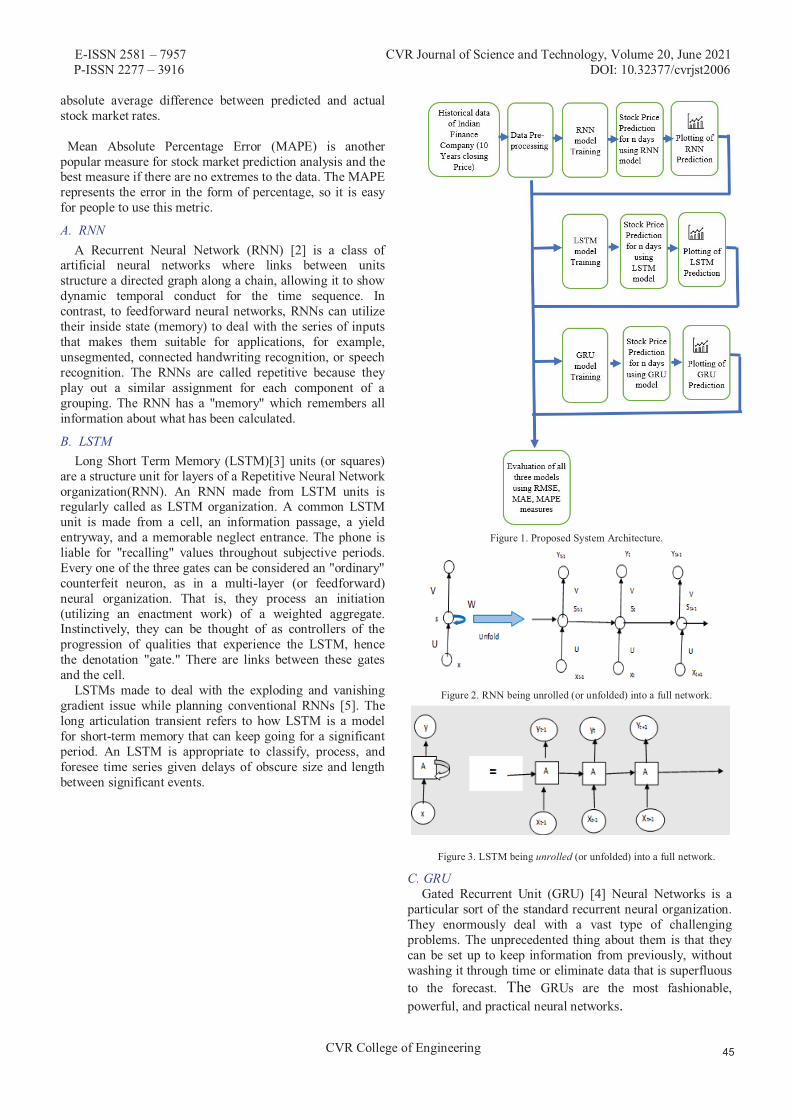
E-ISSN 2581 – 7957 CVR Journal of Science and Technology, Volume 20, June 2021 P-ISSN 2277 – 3916 DOI: 10.32377/cvrjst2006
CVR College of Engineering
absolute average difference between predicted and actual stock market rates. Mean Absolute Percentage Error (MAPE) is another popular measure for stock market prediction analysis and the best measure if there are no extremes to the data. The MAPE represents the error in the form of percentage, so it is easy for people to use this metric.
A. RNN A Recurrent Neural Network (RNN) [2] is a class of
artificial neural networks where links between units structure a directed graph along a chain, allowing it to show dynamic temporal conduct for the time sequence. In contrast, to feedforward neural networks, RNNs can utilize their inside state (memory) to deal with the series of inputs that makes them suitable for applications, for example, unsegmented, connected handwriting recognition, or speech recognition. The RNNs are called repetitive because they play out a similar assignment for each component of a grouping. The RNN has a "memory" which remembers all information about what has been calculated.
B. LSTM Long Short Term Memory (LSTM)[3] units (or squares)
are a structure unit for layers of a Repetitive Neural Network organization(RNN). An RNN made from LSTM units is regularly called as LSTM organization. A common LSTM unit is made from a cell, an information passage, a yield entryway, and a memorable neglect entrance. The phone is liable for "recalling" values throughout subjective periods. Every one of the three gates can be considered an "ordinary" counterfeit neuron, as in a multi-layer (or feedforward) neural organization. That is, they process an initiation (utilizing an enactment work) of a weighted aggregate. Instinctively, they can be thought of as controllers of the progression of qualities that experience the LSTM, hence the denotation "gate." There are links between these gates and the cell.
LSTMs made to deal with the exploding and vanishing gradient issue while planning conventional RNNs [5]. The long articulation transient refers to how LSTM is a model for short-term memory that can keep going for a significant period. An LSTM is appropriate to classify, process, and foresee time series given delays of obscure size and length between significant events.
Figure 1. Proposed System Architecture.
Figure 2. RNN being unrolled (or unfolded) into a full network.
Figure 3. LSTM being unrolled (or unfolded) into a full network.
C. GRU Gated Recurrent Unit (GRU) [4] Neural Networks is a
particular sort of the standard recurrent neural organization. They enormously deal with a vast type of challenging problems. The unprecedented thing about them is that they can be set up to keep information from previously, without washing it through time or eliminate data that is superfluous to the forecast. The GRUs are the most fashionable, powerful, and practical neural networks.

E-ISSN 2581 – 7957 CVR Journal of Science and Technology, Volume 20, June 2021 P-ISSN 2277 – 3916 DOI: 10.32377/cvrjst2006
CVR College of Engineering
It is explicitly intended to avoid long-term dependency [16]. The GRU has fewer parameters than LSTM, thus prepares a model somewhat faster, and also prediction accuracy is more. Examination indicated that the GRU beat the LSTM on the stock forecast.
Figure 4. GRU being unrolled (or unfolded) into a full network.
IV. RESULT ANALYSIS
Result analysis has been done on Power Finance Corporation Ltd., Mahindra and Mahindra Financial Services Ltd., Bajaj Finance Limited stock prices.
A. Power Finance Corporation Ltd. Stock
Power Finance Corporation Ltd. is a Schedule-A Navratna CPSE and is a leading Non-Banking Financial Corporation in the country Incorporated on July 16, 1986. The PFCs enlisted office is situated in New Delhi, and provincial workplaces are located at Mumbai and Chennai [17].
The PFC is under the regulatory control of the Ministry of Power. The PFC has presented the title of a 'Navratna CPSE' in June 2007 and was named Infrastructure Finance Company by the RBI on July 28, 2010. The Power Finance Corporation Ltd. [11], stock price data, has been downloaded from the following web page https://in.finance.yahoo.com/quote/PFC.NS/history/
TABLE I.
SNAPSHOT OF POWER FINANCE CORPORATION LTD. STOCK PRICE DATA.
B. Mahindra & Mahindra Financial Services Limited stock
Mahindra & Mahindra Financial Services Limited is a rustic NBFC settled in Mumbai, India. It is among the top farm truck financers in India and offers a wide scope of monetary items to address fluctuated client necessities. The
Mahindra & Mahindra Financial Services Limited stock price data has been downloaded from the following web page. https://in.finance.yahoo.com/quote/M%26MFIN.NS/history/
TABLE II. SNAPSHOT OF MAHINDRA & MAHINDRA FINANCIAL SERVICES.
C. Bajaj Finance Limited Stock Bajaj Finance Limited is the most broadened and
beneficial non-bank in the country with a wide arrangement of items spread across Consumer, SME and Commercial Lending, and Wealth Management. The Bajaj Finance Limited stock price data has been downloaded from the following web page. https://in.finance.yahoo.com/quote/BAJFINANCE.BO/history/
TABLE III. SNAPSHOT OF BAJAJ FINANCE LIMITED.
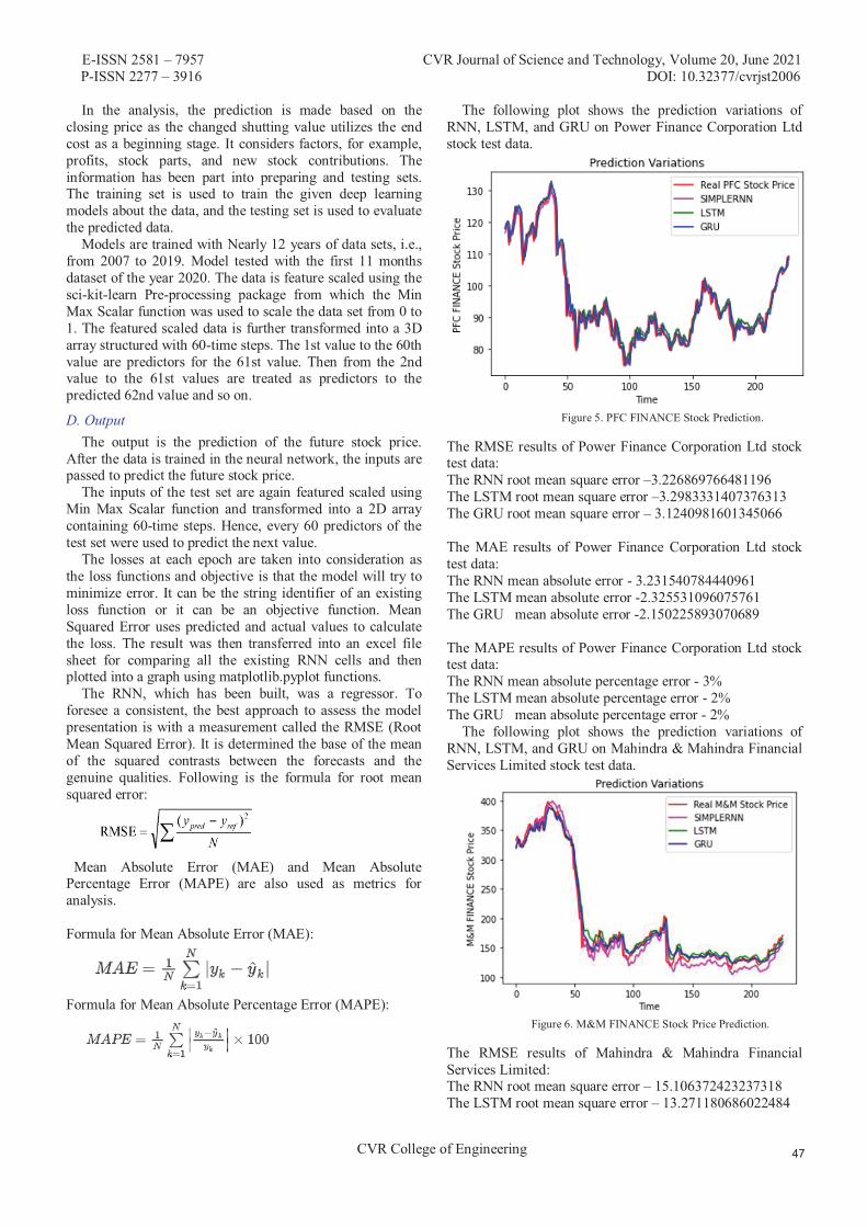
E-ISSN 2581 – 7957 CVR Journal of Science and Technology, Volume 20, June 2021 P-ISSN 2277 – 3916 DOI: 10.32377/cvrjst2006
CVR College of Engineering
In the analysis, the prediction is made based on the closing price as the changed shutting value utilizes the end cost as a beginning stage. It considers factors, for example, profits, stock parts, and new stock contributions. The information has been part into preparing and testing sets. The training set is used to train the given deep learning models about the data, and the testing set is used to evaluate the predicted data.
Models are trained with Nearly 12 years of data sets, i.e., from 2007 to 2019. Model tested with the first 11 months dataset of the year 2020. The data is feature scaled using the sci-kit-learn Pre-processing package from which the Min Max Scalar function was used to scale the data set from 0 to 1. The featured scaled data is further transformed into a 3D array structured with 60-time steps. The 1st value to the 60th value are predictors for the 61st value. Then from the 2nd value to the 61st values are treated as predictors to the predicted 62nd value and so on.
D. Output The output is the prediction of the future stock price.
After the data is trained in the neural network, the inputs are passed to predict the future stock price.
The inputs of the test set are again featured scaled using Min Max Scalar function and transformed into a 2D array containing 60-time steps. Hence, every 60 predictors of the test set were used to predict the next value.
The losses at each epoch are taken into consideration as the loss functions and objective is that the model will try to minimize error. It can be the string identifier of an existing loss function or it can be an objective function. Mean Squared Error uses predicted and actual values to calculate the loss. The result was then transferred into an excel file sheet for comparing all the existing RNN cells and then plotted into a graph using matplotlib.pyplot functions.
The RNN, which has been built, was a regressor. To foresee a consistent, the best approach to assess the model presentation is with a measurement called the RMSE (Root Mean Squared Error). It is determined the base of the mean of the squared contrasts between the forecasts and the genuine qualities. Following is the formula for root mean squared error:
Mean Absolute Error (MAE) and Mean Absolute Percentage Error (MAPE) are also used as metrics for analysis. Formula for Mean Absolute Error (MAE):
Formula for Mean Absolute Percentage Error (MAPE):
The following plot shows the prediction variations of RNN, LSTM, and GRU on Power Finance Corporation Ltd stock test data.
Figure 5. PFC FINANCE Stock Prediction.
The RMSE results of Power Finance Corporation Ltd stock test data: The RNN root mean square error –3.226869766481196 The LSTM root mean square error –3.2983331407376313 The GRU root mean square error – 3.1240981601345066 The MAE results of Power Finance Corporation Ltd stock test data: The RNN mean absolute error - 3.231540784440961 The LSTM mean absolute error -2.325531096075761 The GRU mean absolute error -2.150225893070689 The MAPE results of Power Finance Corporation Ltd stock test data: The RNN mean absolute percentage error - 3% The LSTM mean absolute percentage error - 2% The GRU mean absolute percentage error - 2%
The following plot shows the prediction variations of RNN, LSTM, and GRU on Mahindra & Mahindra Financial Services Limited stock test data.
Figure 6. M&M FINANCE Stock Price Prediction.
The RMSE results of Mahindra & Mahindra Financial Services Limited: The RNN root mean square error – 15.106372423237318 The LSTM root mean square error – 13.271180686022484
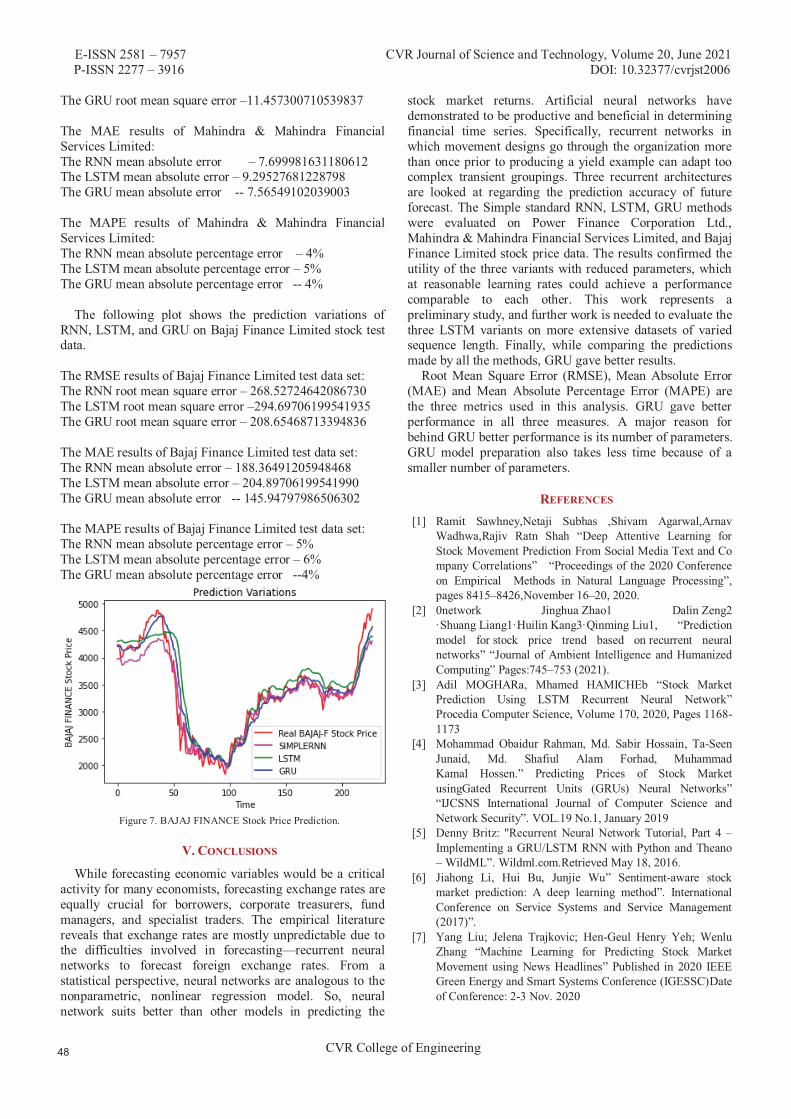
E-ISSN 2581 – 7957 CVR Journal of Science and Technology, Volume 20, June 2021 P-ISSN 2277 – 3916 DOI: 10.32377/cvrjst2006
CVR College of Engineering
The GRU root mean square error –11.457300710539837 The MAE results of Mahindra & Mahindra Financial Services Limited: The RNN mean absolute error – 7.699981631180612 The LSTM mean absolute error – 9.29527681228798 The GRU mean absolute error -- 7.56549102039003 The MAPE results of Mahindra & Mahindra Financial Services Limited: The RNN mean absolute percentage error – 4% The LSTM mean absolute percentage error – 5% The GRU mean absolute percentage error -- 4%
The following plot shows the prediction variations of RNN, LSTM, and GRU on Bajaj Finance Limited stock test data.
The RMSE results of Bajaj Finance Limited test data set: The RNN root mean square error – 268.52724642086730 The LSTM root mean square error –294.69706199541935 The GRU root mean square error – 208.65468713394836 The MAE results of Bajaj Finance Limited test data set: The RNN mean absolute error – 188.36491205948468 The LSTM mean absolute error – 204.89706199541990 The GRU mean absolute error -- 145.94797986506302 The MAPE results of Bajaj Finance Limited test data set: The RNN mean absolute percentage error – 5% The LSTM mean absolute percentage error – 6% The GRU mean absolute percentage error --4%
Figure 7. BAJAJ FINANCE Stock Price Prediction.
V. CONCLUSIONS
While forecasting economic variables would be a critical activity for many economists, forecasting exchange rates are equally crucial for borrowers, corporate treasurers, fund managers, and specialist traders. The empirical literature reveals that exchange rates are mostly unpredictable due to the difficulties involved in forecasting—recurrent neural networks to forecast foreign exchange rates. From a statistical perspective, neural networks are analogous to the nonparametric, nonlinear regression model. So, neural network suits better than other models in predicting the
stock market returns. Artificial neural networks have demonstrated to be productive and beneficial in determining financial time series. Specifically, recurrent networks in which movement designs go through the organization more than once prior to producing a yield example can adapt too complex transient groupings. Three recurrent architectures are looked at regarding the prediction accuracy of future forecast. The Simple standard RNN, LSTM, GRU methods were evaluated on Power Finance Corporation Ltd., Mahindra & Mahindra Financial Services Limited, and Bajaj Finance Limited stock price data. The results confirmed the utility of the three variants with reduced parameters, which at reasonable learning rates could achieve a performance comparable to each other. This work represents a preliminary study, and further work is needed to evaluate the three LSTM variants on more extensive datasets of varied sequence length. Finally, while comparing the predictions made by all the methods, GRU gave better results.
Root Mean Square Error (RMSE), Mean Absolute Error (MAE) and Mean Absolute Percentage Error (MAPE) are the three metrics used in this analysis. GRU gave better performance in all three measures. A major reason for behind GRU better performance is its number of parameters. GRU model preparation also takes less time because of a smaller number of parameters.
REFERENCES [1] Ramit Sawhney,Netaji Subhas ,Shivam Agarwal,Arnav
Wadhwa,Rajiv Ratn Shah “Deep Attentive Learning for Stock Movement Prediction From Social Media Text and Co mpany Correlations” “Proceedings of the 2020 Conference on Empirical Methods in Natural Language Processing”, pages 8415–8426,November 16–20, 2020.
[2] 0network Jinghua Zhao1 Dalin Zeng2 ·Shuang Liang1·Huilin Kang3·Qinming Liu1, “Prediction model for stock price trend based on recurrent neural networks” “Journal of Ambient Intelligence and Humanized Computing” Pages:745–753 (2021).
[3] Adil MOGHARa, Mhamed HAMICHEb “Stock Market Prediction Using LSTM Recurrent Neural Network” Procedia Computer Science, Volume 170, 2020, Pages 1168-1173
[4] Mohammad Obaidur Rahman, Md. Sabir Hossain, Ta-Seen Junaid, Md. Shafiul Alam Forhad, Muhammad Kamal Hossen.” Predicting Prices of Stock Market usingGated Recurrent Units (GRUs) Neural Networks” “IJCSNS International Journal of Computer Science and Network Security”. VOL.19 No.1, January 2019
[5] Denny Britz: "Recurrent Neural Network Tutorial, Part 4 – Implementing a GRU/LSTM RNN with Python and Theano – WildML”. Wildml.com.Retrieved May 18, 2016.
[6] Jiahong Li, Hui Bu, Junjie Wu” Sentiment-aware stock market prediction: A deep learning method”. International Conference on Service Systems and Service Management (2017)”.
[7] Yang Liu; Jelena Trajkovic; Hen-Geul Henry Yeh; Wenlu Zhang “Machine Learning for Predicting Stock Market Movement using News Headlines” Published in 2020 IEEE Green Energy and Smart Systems Conference (IGESSC)Date of Conference: 2-3 Nov. 2020

E-ISSN 2581 – 7957 CVR Journal of Science and Technology, Volume 20, June 2021 P-ISSN 2277 – 3916 DOI: 10.32377/cvrjst2006
CVR College of Engineering
[8] Refenes, A. N., Zapranis, A., & Francis, G. "Stock performance modeling using neural networks: A comparative study with regression models", Neural Networks, vol. 7, no. 2, pp. 375-388, 1994.
[9] Yuling LIN, Haixiang GUO and Jinglu HU “An SVM-based Approach for Stock Market Trend Prediction” The 2013 International Joint Conference on Neural Networks (IJCNN)” ,Date of Conference:August 2013
[10] Yunus YETISl, Halid KAPLAN2, and Mo JAMSHIDI3, “Stock Market Prediction by Using Artificial Neural Network”, Published in: 2014 World Automation Congress (WAC). Date of Conference: 3-7 Aug. 2014.
[11] https://www.pfcindia.com/ [12] Penglei Gao,Rui Zhang , andXi Yang “The Application of
Stock Index Price Prediction with Neural Network” Open access Article, Published: 18 August 2020
[13] https:// www.mahindra.com/ careers/businesses/financial services
[14] WEI YANG “Stock Price Prediction Based on Fuzzy Logic”, “Sixth International Conference on Machine Learning and Cybernetics”, Hong Kong, Date of Conference: 19-22 August 2007.
[15] Aparna Nayak, M. M. Manohara Pai and Radhika M. Pai “Prediction Models for Indian Stock Market”. “Procedia Computer Science” Volume 89 (2016) pages:441 – 449.
[16] Guizhu Shena, Qingping Tana, Haoyu Zhanga, Ping Zenga,Jianjun Xua “Deep Learning with Gated Recurrent Unit Networks for Financial Sequence Predictions”, Procedia Computer Science Volume 131 (2018) Pages:895–903.
[17] Hiransha Ma, Gopalakrishnan E.Ab , Vijay Krishna Menonab , Soman K.P “ NSE Stock Market Prediction Using Deep-Learning Models”,Procedia Computer Science, Volume 132(2018) Pages:1351–1362.
[18] Dr. D. Durga Bhavani, Mir Habeebullah Shah Quadri,Y. Ram Reddy “Dog Breed Identification Using Convolutional Neural Networks on Android” “CVR Journal of Science and Technology” Issue: Vol 17 No 1 (2019).
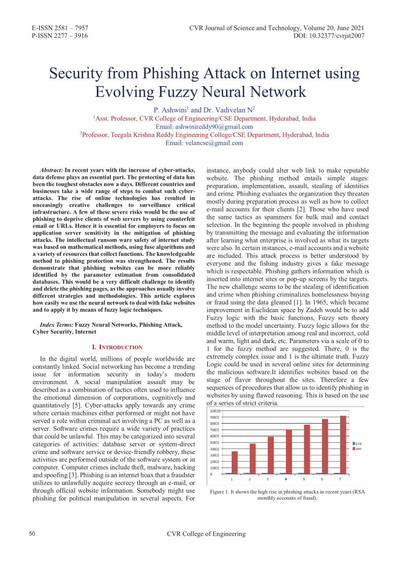
E-ISSN 2581 – 7957 CVR Journal of Science and Technology, Volume 20, June 2021 P-ISSN 2277 – 3916 DOI: 10.32377/cvrjst2007
Security from Phishing Attack on Internet using Evolving Fuzzy Neural Network
P. Ashwini1 and Dr. Vadivelan N2
1Asst. Professor, CVR College of Engineering/CSE Department, Hyderabad, IndiaEmail: [email protected]
2Professor, Teegala Krishna Reddy Engineering College/CSE Department, Hyderabad, IndiaEmail: [email protected]
Abstract: In recent years with the increase of cyber-attacks, data defense plays an essential part. The protecting of data has been the toughest obstacles now a days. Different countries and businesses take a wide range of steps to combat such cyber-attacks. The rise of online technologies has resulted in unceasingly creative challenges to surveillance critical infrastructure. A few of these severe risks would be the use of phishing to deprive clients of web servers by using counterfeit email or URLs. Hence it is essential for employers to focus on application server sensitivity in the mitigation of phishing attacks. The intellectual ransom ware safety of internet study was based on mathematical methods, using fuse algorithms and a variety of resources that collect functions. The knowledgeable method to phishing protection was strengthened. The results demonstrate that phishing websites can be more reliably identified by the parameter estimation from consolidated databases. This would be a very difficult challenge to identify and delete the phishing pages, as the approaches usually involve different strategies and methodologies. This article explores how easily we use the neural network to deal with fake websites and to apply it by means of fuzzy logic techniques.
Index Terms: Fuzzy Neural Networks, Phishing Attack, Cyber Security, Internet
I. INTRODUCTION
In the digital world, millions of people worldwide are constantly linked. Social networking has become a trending issue for information security in today’s modern environment. A social manipulation assault may be described as a combination of tactics often used to influence the emotional dimension of corporations, cognitively and quantitatively [5]. Cyber-attacks apply towards any crime where certain machines either performed or might not have served a role within criminal act involving a PC as well as a server. Software crimes require a wide variety of practices that could be unlawful. This may be categorized into several categories of activities: database server or system-direct crime and software service or device-friendly robbery, these activities are performed outside of the software system or in computer. Computer crimes include theft, malware, hacking and spoofing [3]. Phishing is an internet hoax that a fraudster utilizes to unlawfully acquire secrecy through an e-mail, or through official website information. Somebody might use phishing for political manipulation in several aspects. For
instance, anybody could alter web link to make reputable website. The phishing method entails simple stages: preparation, implementation, assault, stealing of identities and crime. Phishing evaluates the organization they threaten mostly during preparation process as well as how to collect e-mail accounts for their clients [2]. Those who have used the same tactics as spammers for bulk mail and contact selection. In the beginning the people involved in phishing by transmitting the message and evaluating the information after learning what enterprise is involved as what its targets were also. In certain instances, e-mail accounts and a website are included. This attack process is better understood by everyone and the fishing industry gives a fake message which is respectable. Phishing gathers information which is inserted into internet sites or pop-up screens by the targets. The new challenge seems to be the stealing of identification and crime when phishing criminalizes homelessness buying or fraud using the data gleaned [1]. In 1965, which became improvement in Euclidean space by Zadeh would be to add Fuzzy logic with the basic functions, Fuzzy sets theory method to the model uncertainty. Fuzzy logic allows for the middle level of interpretation among real and incorrect, cold and warm, light and dark, etc. Parameters via a scale of 0 to 1 for the fuzzy method are suggested. There, 0 is the extremely complex issue and 1 is the ultimate truth. Fuzzy Logic could be used in several online sites for determining the malicious software.It identifies websites based on the stage of flavor throughout the sites. Therefore a few sequences of procedures that allow us to identify phishing in websites by using flawed reasoning. This is based on the use of a series of strict criteria.
Figure 1. It shows the high rise in phishing attacks in recent years (RSA monthly accounts of fraud).
CVR College of Engineering
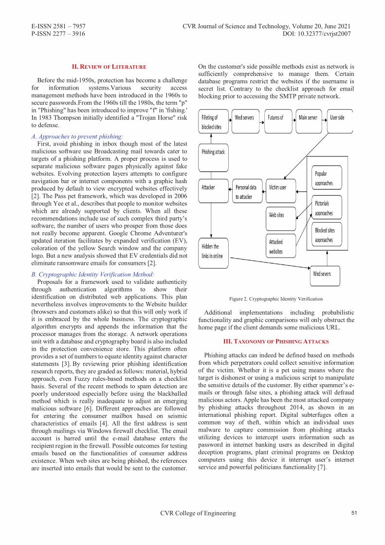
E-ISSN 2581 – 7957 CVR Journal of Science and Technology, Volume 20, June 2021 P-ISSN 2277 – 3916 DOI: 10.32377/cvrjst2007
II. REVIEW OF LITERATURE
Before the mid-1950s, protection has become a challenge for information systems.Various security access management methods have been introduced in the 1960s to secure passwords.From the 1960s till the 1980s, the term "p" in "Phishing" has been introduced to improve "f" in 'fishing.' In 1983 Thompson initially identified a "Trojan Horse" risk to defense.
A. Approaches to prevent phishing: First, avoid phishing in inbox though most of the latest
malicious software use Broadcasting mail towards cater to targets of a phishing platform. A proper process is used to separate malicious software pages physically against fake websites. Evolving protection layers attempts to configure navigation bar or internet components with a graphic hash produced by default to view encrypted websites effectively [2]. The Pass pet framework, which was developed in 2006 through Yee et al., describes that people to monitor websites which are already supported by clients. When all these recommendations include use of such complex third party’s software, the number of users who prosper from those does not really become apparent. Google Chrome Adventurer's updated iteration facilitates by expanded verification (EV), coloration of the yellow Search window and the company logo. But a new analysis showed that EV credentials did not eliminate ransomware emails for consumers [2].
B. Cryptographic Identity Verification Method:Proposals for a framework used to validate authenticity
through authentication algorithms to show their identification on distributed web applications. This plan nevertheless involves improvements to the Website builder (browsers and customers alike) so that this will only work if it is embraced by the whole business. The cryptographic algorithm encrypts and appends the information that the processor manages from the storage. A network operations unit with a database and cryptography board is also included in the protection convenience store. This platform often provides a set of numbers to equate identity against character statements [3]. By reviewing prior phishing identification research reports, they are graded as follows: material, hybrid approach, even Fuzzy rules-based methods on a checklist basis. Several of the recent methods to spam detection are poorly understood especially before using the blackballed method which is really inadequate to adjust an emerging malicious software [6]. Different approaches are followed for entering the consumer mailbox based on seismic characteristics of emails [4]. All the first address is sent through mailings via Windows firewall checklist. The email account is barred until the e-mail database enters the recipient region in the firewall. Possible outcomes for testing emails based on the functionalities of consumer address existence. When web sites are being phished, the references are inserted into emails that would be sent to the customer.
On the customer's side possible methods exist as network is sufficiently comprehensive to manage them. Certain database programs restrict the websites if the username is secret list. Contrary to the checklist approach for email blocking prior to accessing the SMTP private network.
Figure 2. Cryptographic Identity Verification
Additional implementations including probabilistic functionality and graphic comparisons will only obstruct the home page if the client demands some malicious URL.
III. TAXONOMY OF PHISHING ATTACKS
Phishing attacks can indeed be defined based on methods from which perpetrators could collect sensitive information of the victim. Whether it is a pet using means where the target is dishonest or using a malicious script to manipulate the sensitive details of the customer. By either spammer’s e-mails or through false sites, a phishing attack will defraud malicious actors. Apple has been the most attacked company by phishing attacks throughout 2014, as shown in an international phishing report. Digital subterfuges often a common way of theft, within which an individual uses malware to capture commission from phishing attacks utilizing devices to intercept users information such as password in internet banking users as described in digital deception programs, plant criminal programs on Desktop computers using this device it interrupt user’s internet service and powerful politicians functionality [7].
CVR College of Engineering

E-ISSN 2581 – 7957 CVR Journal of Science and Technology, Volume 20, June 2021 P-ISSN 2277 – 3916 DOI: 10.32377/cvrjst2007
Figure 3. Taxonomy of Phishing Attacks
IV. TYPES OF PHISHING
Unless the phishing emails have a unifying theme, its a mask. Intruders modify their contact information seems like it is from somewhere else, make up fake pages that seem through victims relationships, but use odd language features to hide URLs. In specific a strategy to phish your perpetrator aims to choose one of three people.
A. Hand over Sensitive Information:The above notifications are meant to deduce a Security
code frequently used by the perpetrator to expose significant facts. The complete saga of this scheme is to make an enormous financial post, which makes certain halves of the receivers are clients of that company, by bombarding the letter to millions around the world. The customers click on the reference in the text and has been driven to something like a fraudulent portal designed to emulate the Local bank. The perpetrator will now control that identity of the survivor.
B. Download Malware: As several viruses, certain styles of fake attempts are
meant to infect the user towards their own malicious device. Many notifications are "simple directed" and can be submitted to a Security professional, for example with an introduction that would be a career search engine summary. These appendices are mostly .zip or fraudulent encoded software papers from Windows Server. It has been calculated last year that 93% of fake attempts produced. The most prevalent type of malware was hostage goods.
C. Website Forgery: False news sites can be used by Phishing attacks to
gather data. This approach is referred to as websites falsification and occurs in 2 wise packets. Command line techniques are used to mask the exploited link throughout the page settings page as first case of web misrepresentation. Scammers usually mimic reliable organizations message panel logo and insert them next to their deceptive domain URLs. The phablets scripting may also close a pallets link to a photographic settings page replaced that with a real URL to conceal the identification of both the webpages. The
secondary forging approach is by utilizing the vulnerabilities in a database [8].
V. AVAILABLE DIGITAL INTERACTIVE LEARNING SOLUTIONS TO RAISE AWARENESS
Subscribers must usually be knowledgeable in a hope to provide a more trustworthy news network. A technique named the Yoo-hoo sensitization framework is one of the many other alternatives available for raising knowledge about information safety. This resource was primarily expected to boost the growth among computer programmers about the number of interconnected codes in which they operate every day. This method processes details on organization change and thereby strengthens the integrated process of defense. This platform was publicly known among computer programmers about the number of interconnected protocols in which they operate every day. It integrates details on change management and thereby strengthens the online control of defense.
TABLE I. EFFECTS OF CURRENT MEDIA MANIPULATION RECOGNITION
CAMPAIGNS AND TECHNOLOGIES. S.No Aim Methods Findings
1 Acknowledge the compliance causing acute and the Useful-ness Of.
The analysis is fo-cused on random-ized controlled trial of the history.
The final remedy calls for an aware-ness-provoking cultural improve-ment.
2 Gain Knowledge of threats by cognitive technology, identifi-cation, and avoid-ance.
Comprehensive re-view of sufficient data on assaults by social manipulation current methods of identification, avoidance, man-agement of threats and future paths.
Data management protection frame-works are more successful.
3 Consider the possible cyber-attacks styles.
The research is based on an analy-sis of the history.
Multiple sorts of incidents are eas-ier than transmit-ting letters to phishing and im-planted trainings.
4 The feasibility of a safety game is evalu-ated as a successful way to sensitize workers.
A survey was in-troduced and clos-ing interview was done with professors, busi-ness and financial people.
It would be a far more enjoyable and enticing pro-cess. The outcome was far more suc-cessful in increas-ing phishing threat behavior change.
Further strategy to improve respected business is by presenting crucial data, such as encouraging security and intelligence. Close-miss accidents are a significant factor of
CVR College of Engineering
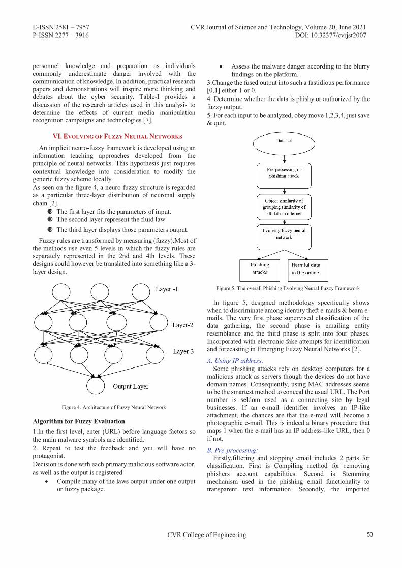
E-ISSN 2581 – 7957 CVR Journal of Science and Technology, Volume 20, June 2021 P-ISSN 2277 – 3916 DOI: 10.32377/cvrjst2007
personnel knowledge and preparation as individuals commonly underestimate danger involved with the communication of knowledge. In addition, practical research papers and demonstrations will inspire more thinking and debates about the cyber security. Table-I provides a discussion of the research articles used in this analysis to determine the effects of current media manipulation recognition campaigns and technologies [7].
VI. EVOLVING OF FUZZY NEURAL NETWORKS
An implicit neuro-fuzzy framework is developed using an information teaching approaches developed from the principle of neural networks. This hypothesis just requires contextual knowledge into consideration to modify the generic fuzzy scheme locally. As seen on the figure 4, a neuro-fuzzy structure is regarded as a particular three-layer distribution of neuronal supply chain [2].
� The first layer fits the parameters of input. � The second layer represent the fluid law. � The third layer displays those parameters output.
Fuzzy rules are transformed by measuring (fuzzy).Most of the methods use even 5 levels in which the fuzzy rules are separately represented in the 2nd and 4th levels. These designs could however be translated into something like a 3-layer design.
Figure 4. Architecture of Fuzzy Neural Network
Algorithm for Fuzzy Evaluation 1.In the first level, enter (URL) before language factors sothe main malware symbols are identified. 2. Repeat to test the feedback and you will have noprotagonist. Decision is done with each primary malicious software actor, as well as the output is registered.
� Compile many of the laws output under one output or fuzzy package.
� Assess the malware danger according to the blurry findings on the platform.
3.Change the fused output into such a fastidious performance[0,1] either 1 or 0. 4. Determine whether the data is phishy or authorized by thefuzzy output. 5. For each input to be analyzed, obey move 1,2,3,4, just save& quit.
Figure 5. The overall Phishing Evolving Neural Fuzzy Framework
In figure 5, designed methodology specifically shows when to discriminate among identity theft e-mails & beam e-mails. The very first phase supervised classification of the data gathering, the second phase is emailing entity resemblance and the third phase is split into four phases. Incorporated with electronic fake attempts for identification and forecasting in Emerging Fuzzy Neural Networks [2].
A. Using IP address: Some phishing attacks rely on desktop computers for a
malicious attack as servers though the devices do not have domain names. Consequently, using MAC addresses seems to be the smartest method to conceal the usual URL. The Port number is seldom used as a connecting site by legal businesses. If an e-mail identifier involves an IP-like attachment, the chances are that the e-mail will become a photographic e-mail. This is indeed a binary procedure that maps 1 when the e-mail has an IP address-like URL, then 0 if not.
B. Pre-processing: Firstly,filtering and stopping email includes 2 parts for
classification. First is Compiling method for removing phishers account capabilities. Second is Stemming mechanism used in the phishing email functionality to transparent text information. Secondly, the imported
CVR College of Engineering

E-ISSN 2581 – 7957 CVR Journal of Science and Technology, Volume 20, June 2021 P-ISSN 2277 – 3916 DOI: 10.32377/cvrjst2007
malware email address is translated into integer numbers (1, 0), while "1" is the legitimate website function and "0" is the fake website function. Then use the e-mail information gathering for E-mail Subject Similarities [4].
C. Spam features: Nearly 90 percent of all e-mails per day are spam. The
Spam Assassin edition 3.2.3.5 could be used in the following review with the predetermined principle and over 40 Conditional functions [5]. It has been tested using thresholds among the most potent technical resources accessible from freeware that could identify spammers. If the notification is labeled as junk is 0 and more or less 5 conditional function determines the average of 1.
VII. RESULTS AND DISCUSSION
Rules which are used in the rule base are divided into 10 layers. Each layer consists of two phishing characteristics rules and is assigned to 0.1 weightage. If the rules in any layer matches with website URL, then it is given 0.1 score. The score of this website is given from 0 to 1. Here 0 indicates low phishy website and 1 indicates high phishy website. The intermediate values between 0 to 1 indicates legitimate phishing. The table II gives different phishing intensity rating of the website for the scores obtained to the given inputs. Based on these results we can finally conclude whether website is fraudulent or the original one. Hence the fuzzy neural network gives one of the efficient ways to derive the website phishiness.
TABLE II. SHOWS THE INTENSITY OF PHISHINESS FROM THE GIVEN URL SCORE
. Frequency of phishing. score
highly Legitimate 0 – 0.1
Legitimate 0.1-0.3
suspicious 0.3 – 0.6
phishy 0.6 – 0.8
Highly phishy 0.8 – 1.0
The Fuzzy logic makes the introductory course of values, which is used to distinguish websites depending mostly on phishers stage that have already been presented in sites using a certain set of measurements and before the laws. Using this method, undefined factors can be processed, and domain operators can then work together to explain these quantities and their relationships. Fuzzy logic often discusses the functionality and the possibility of the website phishing with differential equations.
Accuracy was the parameter for category equations assessment. Informally, Accuracy is the ratio of our photographer's observations. Accuracy = Number of Correct Predictions
Total Number of Predictions
=
TABLE III. SHOWS THE POSSIBLE APPROACHES AND ACCURACY (%).
S.No Approach Accuracy (%)
1 Specifies weight for terms originating through URLs & HTML material includ-
ing trademark
96.3
2 Using a badge picture to define the New website identification through comparing
true and false Websites.
94.5
3 Probabilistic URLs as well as ranks of the websites
95.1
4 A system integrating various technologies has been suggested are KNN and SVM.
91.8
5 FLS (fuzzy Logic System) 97.2
6 FNN (Fuzzy Neural Networks) 99.8
This article shows an innovative solution directed at URL as well as the anger logic process to achieve the advantages of a flimsy principle scheme. This method is used in 5 steps: choose the URL functionality, calculation of 6 probabilistic variables, calculation of 12 fluid prices for 6 participation probabilistic reasoning technologies; Averaging 6 fluid phishing accounting knowledge (MP) and average 6 fluctuated principles for a legal language mark. The MP & ML quantities are linked to the New website classification. The solution was tested for 10,660 websites which includes 5,660 identity theft websites and 5,000 legal websites. Hence Accuracy of the proposed algorithm was 99.8%.
Figure 6. Accuracy of different Approaches
Neuro-Fuzzy method includes inductive reasoning of neural network rather than single fluid framework. Provided there is an extraction of a 300-value information source from six valid website regulation, consumer, credit cards, pop-up screens and client. The suggested framework was also used
CVR College of Engineering

E-ISSN 2581 – 7957 CVR Journal of Science and Technology, Volume 20, June 2021 P-ISSN 2277 – 3916 DOI: 10.32377/cvrjst2007
for preparation and research through Point Mutation Bridge. The fuzzy system has five comprehension and validation features, including input nodes, flushing, directive, centralization, and defecation. The inference was that the website factors does not influence the decision and only the new website has fool fighter features. Utilization of established global theory has become one of the most efficient means of achieving phishiness of a blog site. A description of several titles is given in Table I.
VIII. CONCLUSIONS
Phishing is a cyberattack where attackers target through Several alternatives. Phishing commonly utilizes internet for illegal purposes through phishing companies and e-mail spoofing.Electronic trades are important in this modern age of social Media which generate bad experiences. Their research allows new investors to know the past, recent patterns, and failures of alternative problems. Trojans Sites can indeed be predicted using fuzzy neural network models. Previous studies using different methods for data processing identification have been performed for predicting spam emails, but the failure rate of these techniques has been quite strong. This helps efficiency to be increased with faded neural systems as the failure is decreased and the accuracy is improved. We think this approach fits and has smaller margin of failure.
REFERENCES [1] L. Wenyin, G. Huang, L. Xiaoyue, X. Deng, and Z. Min,
“Phishing web page detection,” in Document Analysis and Recognition, 2005. Proceedings.Eighth International Confer-ence on. IEEE, pp. 560–564.
[2] B. B. Gupta, A. Tewari, A. K. Jain, and D. P. Agrawal, “Fighting against phishing attacks: state of the art and future challenges,” in Neural Computing and Applications, 2016.
[3] Maher Aburrous, M.A. Hossain, Keshav Dahal,Fadi Thab-tah “Predicting Phishing Websitesusing Classification Min-ing Techniques with Experimental Case Studies”, Seventh International Conference on Information Technology, 2010.
[4] Maher Aburrous, M.A. Hossain, Keshav Dahal,Fadi Thabtah “Intelligent phishing detectionsystem for e-banking using fuzzy data mining”,Expert Systems with Applications: AnIn-ternational Journal Volume 37 Issue 12,December, 2010.
[5] Zhou, Yu, et al. "Visual Similarity Based Anti-phishing with the Combination of Local and Global Features." Trust, Secu-rity and Privacy in Computing and Communications (Trust-Com), 2014 IEEE 13th International Conference on. IEEE, 2014.
[6] Yu, Weider D., Shruti Nargundkar, and NagapriyaTiruthani. "A phishing vulnerability analysis of web-based systems." Computers and Communications, 2008.ISCC 2008. IEEE Symposium on. IEEE, 2008.
[7] P.A. Barraclough, M.A. Hossain, M.A. Tahir b, G. Sexton, N.Aslam, “Intelligent phishing detection and protection scheme for online transactions”, Expert Systems with Appli-cations 40 (2013) 4697–4706.
[8] Gaurav Kumar Tak and Gaurav Ojha, “Multi-Level Parsing Based Approach against Phishing Attacks with the Help of Knowledge Bases”, International Journal of Network security & its applications (IJNSA), Vol.5, No.6, November2013.
CVR College of Engineering
E-ISSN 2581 – 7957 CVR Journal of Science and Technology, Volume 20, June 2021P-ISSN 2277 – 3916 DOI: 10.32377/cvrjst2008
CVR College of Engineering
Low Power Fast and Accurate Localization Algorithm in Wireless Sensor Networks
Dr. Gaurav Sharma1 and Dr. Manjeet Kharub2
1Asst. Prof , CVR College of Engineering/ECE Department, Hyderabad, IndiaEmail: [email protected]
2Assoc. Prof., CVR College of Engineering/Mechanical Engg. Department, Hyderabad, IndiaEmail: [email protected]
Abstract: Finding precise node localization is one of the critical issues in wireless sensor networks (WSNs), as the nodes are generally deployed randomly in the area of interest and without location stamp of the event, there is no use of that particular information. In this paper, a range-free localization algorithm called Horizontal-Vertical (H-V) scan method is presented which works mainly on collinearity concept. This method firstly estimates the collinearity of anchor nodes and rules out those anchor nodes which are collinear for location estimation of target nodes. By ruling out collinear anchor nodes, location is calculated by other than these ruled out anchor nodes through trilateration method which improves the localization accuracy. A new trajectory is also proposed for this method which improves coverage, accuracy and time for calculating localization. Simulation results show that the proposed method performs better in terms of localization accuracy, than the existing similar range-free localization methods.
Index Terms: Localization, Collinearity concept, H-V scan method, WSN, Localization accuracy.
I. INTRODUCTION
Wireless sensor networks are widely used for large-scale networks having very small embedded devices called as sensor nodes with sensing, transmitting, receiving and computational capabilities [1–3]. These sensor nodes are small in size with limited power, memory and communication bandwidth. Therefore, efficient uses of these resources become necessary for proper working of WSNs for a long time. Sensor nodes are mostly expected to be aware of their positions in network area. For instance, the location of occurrence is essential in applications which are designed to detect some phenomena like fire detection. Further, since some routing protocols are position-based, that must know the position of each node in the network [1]. Therefore, calculating or obtaining the position of the nodes in the network is a challenge in WSNs which is called localization [2].
In recent years, a large body of research has been conducted regarding the estimation of the node position in the network area and several localization methods were employed in WSNs in this regard. As shown in Fig. 1, these methods are mainly categorized into centralized anddistributed (self-localization) localization techniques. In the first technique, the localization process and its calculations are obtained by the Base Station while in the latter, each node separately calculates its position [3]. Therefore, different studies concentrated on anchor-based localization
in which a few numbers of anchor nodes are equipped with GPS receivers [4].
However, energy consumption and overhead cost are reported as two main drawbacks of GPS based localization methods [5]. The localization methods can be divided into anchor-free or anchor-based methods based on the use of anchor nodes. Moreover, these anchor nodes can be static or mobile for traversing the network region [6].Eventually, the localization algorithms which estimate and calculate the node positions are classified into range-free and range-based groups [7]. The position of nodes in range-free techniques is estimated based on exchange information among nodes known as connectivity information [8]. However, the location of nodes in range-based techniques is obtained by distance or angle of multiple nodes in the network. Accordingly, these methods impose extra cost, volume and energy usage to the network, since they must calculate the distance or angle among nodes [9].
In range-free methods, the Distance Vector by Hopcounting (DV-hop) algorithm [7] is considered as a standard technique for obtaining the necessary information for localization. In contrast, range-based methods use several approaches to calculate the distance or angle among nodes in order to estimate the location of each node. These techniques include the Time of Arrival ToA) [10], Time Difference of Arrival (TDoA) [11-12], Received Signal Strength Indicator (RSSI) [13], techniques for calculating distance and the Angle of Arrival of the signal (AoA) [14],technique for calculating angle ,and also hybrid methods that are combination of the abovementioned techniques [15],[16]. The present study focuses on random deployment of static sensor nodes which used one mobile anchor node as a reference node to calculate the nodes positions in network area.
II. RELATED WORKS
As previously mentioned, localization algorithms are categorized into range-based and range-free methods. The relevant localization algorithms presented in the literature are provided in the following paragraphs.
First, several studies in the area of the range-free method are discussed. Safa [23] proposed an algorithm based on theDV-hop method. Accordingly, the anchor nodes are located on a circle, or a semi-circle around the desired area in order to improve the localization accuracy. This placement strategy is suitable for military surveillance or tracking applications and environmental monitoring. The current
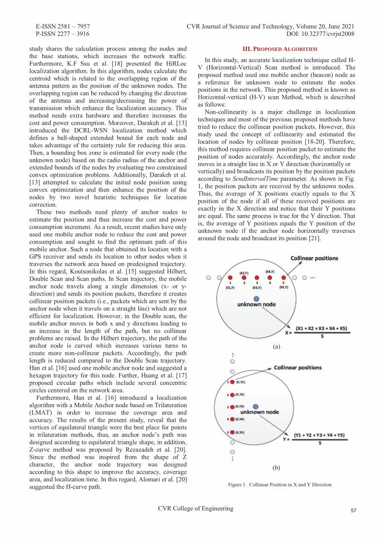
E-ISSN 2581 – 7957 CVR Journal of Science and Technology, Volume 20, June 2021 P-ISSN 2277 – 3916 DOI: 10.32377/cvrjst2008
CVR College of Engineering
study shares the calculation process among the nodes and the base stations, which increases the network traffic. Furthermore, K.F Ssu et al. [18] presented the HiRLoc localization algorithm. In this algorithm, nodes calculate the centroid which is related to the overlapping region of the antenna pattern as the position of the unknown nodes. The overlapping region can be reduced by changing the direction of the antenna and increasing/decreasing the power of transmission which enhance the localization accuracy. This method needs extra hardware and therefore increases the cost and power consumption. Moreover, Darakeh et al. [13] introduced the DCRL-WSN localization method which defines a ball-shaped extended bound for each node and takes advantage of the certainty rule for reducing this area. Then, a bounding box zone is estimated for every node (the unknown node) based on the radio radius of the anchor and extended bounds of the nodes by evaluating two constrained convex optimization problems. Additionally, Darakeh et al. [13] attempted to calculate the initial node position using convex optimization and then enhance the position of the nodes by two novel heuristic techniques for location correction.
These two methods need plenty of anchor nodes to estimate the position and thus increase the cost and power consumption increment. As a result, recent studies have only used one mobile anchor node to reduce the cost and power consumption and sought to find the optimum path of this mobile anchor. Such a node that obtained its location with a GPS receiver and sends its location to other nodes when it traverses the network area based on predesigned trajectory. In this regard, Koutsonikolas et al. [15] suggested Hilbert, Double Scan and Scan paths. In Scan trajectory, the mobile anchor node travels along a single dimension (x- or y-direction) and sends its position packets, therefore it creates collinear position packets (i.e., packets which are sent by the anchor node when it travels on a straight line) which are not efficient for localization. However, in the Double scan, the mobile anchor moves in both x and y directions leading to an increase in the length of the path, but no collinear problems are raised. In the Hilbert trajectory, the path of the anchor node is curved which increases various turns to create more non-collinear packets. Accordingly, the path length is reduced compared to the Double Scan trajectory. Han et al. [16] used one mobile anchor node and suggested a hexagon trajectory for this node. Further, Huang et al. [17] proposed circular paths which include several concentric circles centered on the network area.
Furthermore, Han et al. [16] introduced a localization algorithm with a Mobile Anchor node based on Trilateration (LMAT) in order to increase the coverage area and accuracy. The results of the present study, reveal that the vertices of equilateral triangle were the best place for points in trilateration methods, thus, an anchor node’s path was designed according to equilateral triangle shape, in addition, Z-curve method was proposed by Rezazadeh et al. [20]. Since the method was inspired from the shape of Z character, the anchor node trajectory was designed according to this shape to improve the accuracy, coverage area, and localization time. In this regard, Alomari et al. [20] suggested the H-curve path.
III. PROPOSED ALGORITHM
In this study, an accurate localization technique called H-V (Horizontal-Vertical) Scan method is introduced. The proposed method used one mobile anchor (beacon) node as a reference for unknown node to estimate the nodes positions in the network. This proposed method is known as Horizontal-vertical (H-V) scan Method, which is described as follows:
Non-collinearity is a major challenge in localization techniques and most of the previous proposed methods have tried to reduce the collinear position packets. However, this study used the concept of collinearity and estimated the location of nodes by collinear position [18-20]. Therefore, this method requires collinear position packet to estimate the position of nodes accurately. Accordingly, the anchor node moves in a straight line in X or Y direction (horizontally or vertically) and broadcasts its position by the position packets according to SendIntervalTime parameter. As shown in Fig. 1, the position packets are received by the unknown nodes. Thus, the average of X positions exactly equals to the X position of the node if all of these received positions are exactly in the X direction and notice that their Y positions are equal. The same process is true for the Y direction. That is, the average of Y positions equals the Y position of the unknown node if the anchor node horizontally traverses around the node and broadcast its position [21].
(a)
(b)
Figure 1. Collinear Position in X and Y Direction
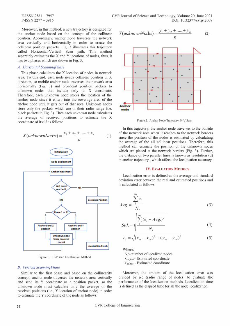
E-ISSN 2581 – 7957 CVR Journal of Science and Technology, Volume 20, June 2021 P-ISSN 2277 – 3916 DOI: 10.32377/cvrjst2008
CVR College of Engineering
Moreover, in this method, a new trajectory is designed for the anchor node based on the concept of the collinear position. Accordingly, anchor node traverses the network area vertically and horizontally in order to create the collinear position packets. Fig. 3 illustrates this trajectory called Horizontal-Vertical Scan path. This method separately estimates the X and Y locations of nodes, thus, it has two phases which are shown in Fig. 3.
A. Horizontal ScanningPhase This phase calculates the X location of nodes in network
area. To this end, each node needs collinear position in X direction, so mobile anchor node traverses the network area horizontally (Fig. 3) and broadcast position packets to unknown nodes that include only its X coordinate. Therefore, each unknown node stores the location of the anchor node since it enters into the coverage area of the anchor node until it gets out of that area. Unknown nodes store only the packets which are in their radio range (i.e. black packets in Fig. 3). Then each unknown node calculates the average of received positions to estimate the X coordinate of itself as follow:
nxxxesunknownNodX n���
�.....
)( 21 (1)
Figure 1. H-V scan Localization Method
B. Vertical ScanningPhase Similar to the first phase and based on the collinearity
concept, anchor node traverses the network area vertically and send its Y coordinate as a position packet, so the unknown node must calculate only the average of the received positions (i.e., Y location of anchor node) in order to estimate the Y coordinate of the node as follows:
nyyyesunknownNodY n���
�.....
)( 21 (2)
Figure . Anchor Node Trajectory: H-V Scan
In this trajectory, the anchor node traverses to the outside of the network area when it reaches to the network borders since the position of the nodes is estimated by calculating the average of the all collinear positions. Therefore, this method can estimate the position of the unknown nodes which are placed at the network borders (Fig. 3). Further, the distance of two parallel lines is known as resolution (d) in anchor trajectory , which affects the localization accuracy.
IV. EVALUATION METRICS
Localization error is defined as the average and standard deviation error between the real and estimated positions and is calculated as follows:
l
N
i
N
eAvg
l
�� 1. (3)
l
N
i
N
AvgeStd
l
� �� 1
2.)(. (4)
22 )()( acesacesi yyxxe ���� (5)
Where: Nl:- number of localized nodes xes,yes:- Estimated coordinate xac,yac:- Estimated coordinate
Moreover, the amount of the localization error was divided by (radio range of nodes) to evaluate the performance of the localization methods. Localization time is defined as the elapsed time for all the node localization.
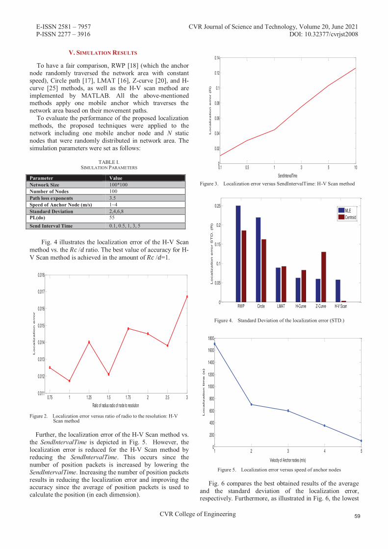
E-ISSN 2581 – 7957 CVR Journal of Science and Technology, Volume 20, June 2021 P-ISSN 2277 – 3916 DOI: 10.32377/cvrjst2008
CVR College of Engineering
To have a fair comparison, RWP [18] (which the anchor node randomly traversed the network area with constant speed), Circle path [17], LMAT [16], Z-curve [20], and H-curve [25] methods, as well as the H-V scan method are implemented by MATLAB. All the above-mentioned methods apply one mobile anchor which traverses the network area based on their movement paths.
To evaluate the performance of the proposed localization methods, the proposed techniques were applied to the network including one mobile anchor node and N static nodes that were randomly distributed in network area. The simulation parameters were set as follows:
TABLE I. SIMULATION PARAMETERS
Parameter Value Network Size 100*100 Number of Nodes 100 Path loss exponents 3.5 Speed of Anchor Node (m/s) 1~4 Standard Deviation 2,4,6,8 PL(do) 55 Send Interval Time 0.1, 0.5, 1, 3, 5
Fig. 4 illustrates the localization error of the H-V Scan method vs. the / ratio. The best value of accuracy for H-V Scan method is achieved in the amount of / =1.
0.75 1 1.25 1.5 1.75 2 2.5 30.011
0.012
0.013
0.014
0.015
0.016
0.017
0.018
Ratio of radius radio of node to resolution
Lo
ca
liza
tio
n e
rro
r
Figure 2. Localization error versus ratio of radio to the resolution: H-V Scan method
Further, the localization error of the H-V Scan method vs. the SendIntervalTime is depicted in Fig. 5. However, the localization error is reduced for the H-V Scan method by reducing the SendIntervalTime. This occurs since the number of position packets is increased by lowering the SendIntervalTime. Increasing the number of position packets results in reducing the localization error and improving the accuracy since the average of position packets is used to calculate the position (in each dimension).
0.1 0.5 1 3 5 100
0.02
0.04
0.06
0.08
0.1
0.12
0.14
SendIntervalTime
Lo
ca
liza
tio
n e
rro
r (
R)
Figure 3. Localization error versus SendIntervalTime: H-V Scan method
RWP Circle LMAT H-Curve Z-Curve H-V Scan0
0.05
0.1
0.15
0.2
0.25L
oca
liza
tio
n e
rro
r S
TD
. (R
)MLECentroid
Figure 4. Standard Deviation of the localization error (STD.)
1 2 3 4 50
200
400
600
800
1000
1200
1400
1600
1800
Velocity of Anchor nodes (m/s)
Lo
ca
liza
tio
n tim
e (
s)
Figure 5. Localization error versus speed of anchor nodes
Fig. 6 compares the best obtained results of the average and the standard deviation of the localization error, respectively. Furthermore, as illustrated in Fig. 6, the lowest
V. SIMULATION RESULTS

E-ISSN 2581 – 7957 CVR Journal of Science and Technology, Volume 20, June 2021 P-ISSN 2277 – 3916 DOI: 10.32377/cvrjst2008
CVR College of Engineering
value of localization error of H-V Scan is about 0.01R which is far less than all other methods.
The localization time is another critical parameter used to evaluate the performance of localization methods. This parameter is inversely proportional to the speed of the anchor node, thus the localization time decreases if the speed of the anchor node increases. The localization time of the H-V Scan method vs. the speed of the anchor node (V) is shown in Fig. 7. As expected, localization time reduced when the speed of the anchor node increased.
VI. CONCLUSIONS
H-V Scan localization technique was introduced in the present study in order to estimate the position of sensor nodes in the network area. This method suggested a new optimum trajectory for anchor node to traverse the network area. In addition, it used different algorithms to calculate the position of the nodes. H-V scan method is range-free method which used collinearity feature and calculated the location of nodes in the network based on collinearity concept. The simulation results indicated that this method can significantly improve the accuracy of localization with time overheads compared to other methods (i.e., RWP, Circle, LMAT, Z-curve, and H-curve) used in other studies.
REFERENCES [1] G. Mao, B. Fidan, and B. D. O. Anderson, “Wireless sensor
network localization techniques,” Comput. Networks, vol. 51, no. 10, pp. 2529–2553, Jul. 2007.
[2] A. Pal, “Localization algorithms in wireless sensor networks: Current approaches and future challenges,” Netw. Protoc. algorithms, vol. 2, no. 1, pp. 45–73, 2010.
[3] T. J. S. Chowdhury, C. Elkin, V. Devabhaktuni, D. B. Rawat, and J. Oluoch, “Advances on localization techniques for wireless sensor networks: A survey,” Comput. Networks, vol. 110, pp. 284–305, Dec. 2016.
[4] U. Nazir, N. Shahid, M. A. Arshad, and S. H. Raza, “Classification of localization algorithms for wireless sensor network: A survey,” in 2012 International Conference on Open Source Systems and Technologies, 2012, pp. 1–5.
[5] Yun Wang, Xiaodong Wang, Demin Wang, and D. P. Agrawal, “Range-Free Localization Using Expected Hop Progress in Wireless Sensor Networks,” IEEE Trans. Parallel Distrib. Syst., vol. 20, no. 10, pp. 1540–1552, Oct. 2009.
[6] G. Han, H. Xu, T. Q. Duong, J. Jiang, and T. Hara, “Localization algorithms of Wireless Sensor Networks: a survey,” Telecommun. Syst., vol. 52, no. 4, pp. 2419–2436, Apr. 2013.
[7] D. Niculescu and B. Nath, “DV Based Positioning in Ad Hoc Networks,” Telecommun. Syst., vol. 22, no. 1/4, pp. 267–280, 2003.
[8] G. Sharma and A. Kumar, “Fuzzy logic based 3D localization in wireless sensor networks using invasive weed and bacterial foraging optimization,” Telecommunication Systems, vol. 67, no. 2, pp. 149–162, May 2017.
[9] G. Sharma, & A. Kumar, “Improved DV-Hop localization algorithm using teaching learning based optimization for
wireless sensor networks”. Telecommunication Systems, vol. 67, no. 2, pp. 163-178, 2017.
[10] S. Go and J.-W. Chong, “Improved TOA-Based Localization Method with BS Selection Scheme for Wireless Sensor Networks,” ETRI J., vol. 37, no. 4, pp. 707–716, Aug. 2015.
[11] P. K. Sahu, E. H.-K. Wu, and J. Sahoo, “DuRT: Dual RSSI Trend Based Localization for Wireless Sensor Networks,” IEEE Sens. J., vol. 13, no. 8, pp. 3115–3123, Aug. 2013.
[12] P. Kułakowski, J. Vales-Alonso, E. Egea-López, W. Ludwin, and J. García-Haro, “Angle of- arrival localization based on antenna arrays for wireless sensor networks,” Comput. Electr. Eng., vol. 36, no. 6, pp. 1181–1186, Nov. 2010.
[13] F. Darakeh, G.-R. Mohammad-Khani, and P. Azmi, “CRWSNP: cooperative range-free wireless sensor network positioning algorithm,” Wirel. Networks, vol. 24, no. 8, pp. 2881–2897, Nov. 2018.
[14] Sharma, G., & Kharub, M. (2019). Enhanced Range Free Localization in Wireless Sensor Networks. CVR Journal of Science and Technology, 16(1), 26-31.
[15] D. Koutsonikolas, S. M. Das, and Y. C. Hu, “Path planning of mobile landmarks for localization in wireless sensor networks,” Comput. Commun., vol. 30, no. 13, pp. 2577– 2592, Sep. 2007.
[16] G. Han, C. Zhang, J. Lloret, L. Shu, and J. J. P. C. Rodrigues, “A mobile anchor assisted localization algorithm based on regular hexagon in wireless sensor networks.,” ScientificWorldJournal., vol. 2014, Jul. 2014.
[17] R. Huang and G. V. Zaruba, “Static Path Planning for Mobile Beacons to Localize Sensor Networks,” in Fifth Annual IEEE International Conference on Pervasive Computing and Communications Workshops (PerComW’07), 2007, pp. 323–330.
[18] K.-F. Ssu, C.-H. Ou, and H. C. Jiau, “Localization With Mobile Anchor Points in Wireless Sensor Networks,” IEEE Trans. Veh. Technol., vol. 54, no. 3, pp. 1187–1197, May 2005.
[19] G. Sharma and A. Kumar, “Modified Energy-Efficient Range-Free Localization Using Teaching–Learning-Based Optimization for Wireless Sensor Networks,” IETE Journal of Research, vol. 64, no. 1, pp. 124–138, Jul. 2017.
[20] J. Rezazadeh, M. Moradi, A. S. Ismail, and E. Dutkiewicz, “Superior Path Planning Mechanism for Mobile Beacon-Assisted Localization in Wireless Sensor Networks,” IEEE Sens. J., vol. 14, no. 9, pp. 3052–3064, Sep. 2014.
[21] A. Coluccia and A. Fascista, “On the Hybrid TOA/RSS Range Estimation in Wireless Sensor Networks,” IEEE Trans. Wirel. Commun., vol. 17, no. 1, pp. 361–371, Jan. 2018.
[22] N. Ben Halima and H. Boujemâa, “3D WLS hybrid and non hybrid localization using TOA, TDOA, azimuth and elevation,” Telecommun. Syst., pp. 1–8, Jun. 2018.
[23] H. Safa, “A novel localization algorithm for large scale wireless sensor networks,” Comput. Commun., vol. 45, pp. 32–46, Jun. 2014.
[24] G. Sharma, & A. Kumar, “Dynamic Range Normal Bisector Localization Algorithm for Wireless Sensor Networks”. Wireless Personal Communications, vol. 9, no. 3, pp. 4529-4549, 2017.
[25] A. Alomari, F. Comeau, W. Phillips, and N. Aslam, “New path planning model for mobile anchor-assisted localization in wireless sensor networks,” Wirel. Networks, vol. 24, no. 7, pp. 2589–2607, Oct. 2018.
E-ISSN 2581 – 7957 CVR Journal of Science and Technology, Volume 20, June 2021 P-ISSN 2277 – 3916 DOI: 10.32377/cvrjst2009
CVR College of Engineering
FPGA Realization of Logic Gates using Neural Networks
R. Ganesh1 and D. Bhanu Prakash2 1Assoc. Professor, CVR College of Engineering /ECE Department, Hyderabad, India
Email: [email protected] 2Assoc. Professor, CVR College of Engineering /ECE Department, Hyderabad, India
Email: [email protected]
Abstract: The real time systems are designed by using analog and digital sub systems with control logic. In the design of digital sub systems the logic gates are the major building blocks. The Neural Networks found many applications in the areas of pattern recognition, prediction, artificial intelligence and other applications. Most of the Neural Network designs are realized by using software domain and hardware domains. This paper presents the hardware realization of logic gates using Neural Network.
The logic gates like NAND, AND, NOR, OR, NOT, BUFFER are realized by using single layer neural network. The XNOR and XOR logic gates are realized by using structural representation of neural network based universal NAND gates. All the logic gates are realized by using Verilog HDL with Xilinx Vivado Design suite targeting for Xilinx Zynq-7000 SoC Evaluation Board. The Neural Network based logic gates are simulated for different test cases.
Index Terms: Neural Network, Logic Gate, Zynq-7000 SoC, Verilog HDL, Xilinx Vivado EDA tool.
. INTRODUCTION
The present modern real time systems are designed by using Digital, Analog, Mixed and co-design subsystems, to meet non functional constraints like area, speed, power, cost and other parameters. In all these subsystems the digital design plays an important role in meeting the non functional constraints.
The Neural Networks (NN) found many applications in the areas of pattern recognition, prediction, artificial intelligence, and other applications [1]. Most of the Neural Network designs are realized by using software domain with mainly concentrating on the application input, outputs and not on the internal structure of the design. This application oriented design of software realization has an advantage of simple coding, low cost with a limitation of slower execution time.
The limitation of software realization of NN can be overcome by using hardwar realization using Microprocessor, Digital Signal Processing (DSP) and Very Large Scale Integration (VLSI). The Neural Network design requires lot of parallel computations. The Microprocessors and DSP are not suitable for parallel execution of NN systems. Hence, to design Neural Network systems the VLSI is considered as the best method for parallelism [2].
The design approaches for VLSI systems is shown in Figure 1. The design of VLSI systems can be divided into three sub system domains. i.e. Digital VLSI system domain, Analog VLSI system domain and Mixed VLSI system domains [3].
Figure 1. Design approaches in VLSI Design
The digital VLSI systems are realized by using textual hardware languages like Very High Speed Integrated Circuit Hardware Description Language (VHDL), Verilog HDL, System Verilog etc. The Analog VLSI systems are realized by using transistors based schematic representations. The mixed VLSI systems are realized by using the combination of both Analog and Digital design entry representations. The Digital VLSI is divided into FPGA and standard cell-based designs. The Field Programmable Gate Array (FPGA) based design is having the feature of re-programmability, whereas the standard cell-based VLSI require the foundry based standard cell library and it is not having the feature of re-programmability. The Analog VLSI systems using transistors is done by using a full custom based approach, which does not use any HDL coding and re-programmability.
The FPGA based designs are well suited for the realization of digital design systems due to its flexibility of logic gates realization, HDL entry and re-programmability features. The logic gates are the major building blocks in the realization of digital design system. All these logic gates i.e. NAND, AND, NOR, OR, XNOR, XOR, NOT and BUFFER can be realized by using different design methodologies based on the targeted application. The design methodologies are selected to meet the logic functionality equation and truth table of the corresponding logic gate. All these logic gates are used as the basic building blocks for realizing the complex system.
This paper presents realization of neural network based logic gates i.e. NAND, AND, NOR, OR, XNOR, XOR, NOT and BUFFER using FPGA. The chapter II presents the concepts of Neural Networks along with the types of Neural Network architectures. The chapter III presents design methodology of Neural Networks based logic gates. The chapter IV gives the design and realization of NN based logic gates; the chapter V gives the simulation results. The conclusion is presented in chapter VI followed by references.
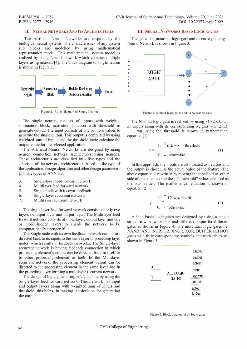
E-ISSN 2581 – 7957 CVR Journal of Science and Technology, Volume 20, June 2021 P-ISSN 2277 – 3916 DOI: 10.32377/cvrjst2009
CVR College of Engineering
. NEURAL NETWORKS AND ITS ARCHITECTURES
The Artificial Neural Networks are inspired by the biological neural systems. The characteristics of any system sub blocks are modelled by using mathematical representation model. This mathematical system model is realized by using Neural network which contains multiple layers using neurons [4]. The block diagram of single neuron is shown in Figure 2.
Figure 2. Block diagram of Single Neuron
The single neuron consists of inputs with weights, summation block, activation function with threshold to generate output. The input consists of one or more values to generate the single output. This output is computed by using weighted sum of inputs and the threshold logic calculate the output value for the selected application. The Artificial Neural Networks are designed by using neuron connection network architectures using neurons. These architectures are classified into five types and the selection of the network architecture is based on the type of the application, design algorithm and other design parameters [5]. The types of ANN are:
3. Single-layer feed forward network4. Multilayer feed forward network5. Single node with its own feedback6. Single-layer recurrent network7. Multilayer recurrent network
The single layer feed forward network consists of only two layers i.e. input layer and output layer. The Multilayer feed forward network consists of input layer, output layer and one or more hidden layers to enable the network to be computationally stronger [6]. The Single node with its own feedback network outputs are directed back to its inputs to the same layer or preceding layer nodes, which results in feedback networks. The Single-layer recurrent network is having feedback connection in which processing element’s output can be directed back to itself or to other processing element or both. In the Multilayer recurrent network, the processing element output can be directed to the processing element in the same layer and in the preceding layer forming a multilayer recurrent network. The design of logic gates using ANN is done by using the Single-layer feed forward network. This network has input and output layers along with weighted sum of inputs and threshold, this helps in making the decision for generating the output.
. NEURAL NETWORKS BASED LOGIC GATES
The general structure of logic gate and its corresponding Neural Network is shown in Figure 3.
Figure 3. N-input logic gates and its Neural network
The N-input logic gate is realized by using x1,x2,x3, …., xn inputs along with its corresponding weights w1,w2,w3, ….., wn using the threshold is shown in mathematical equation (1).
1, if Ʃ wixi > threshold y = (1)
0, otherwise
In this approach, the inputs are also treated as neurons and the output is chosen as the actual value of the feature. The above equation is rewritten by moving the threshold to other side of the equation and these “-threshold” values are used as the bias values. The mathematical equation is shown in equation (2).
1, if Ʃ wixi +b >0 y = (2)
0, otherwise
All the basic logic gates are designed by using a single structure with two inputs and different output for different gates as shown in Figure 4. The individual logic gates i.e. NAND, AND, NOR, OR, XNOR, XOR, BUFFER and NOT gates with their corresponding symbols and truth tables are shown in Figure 5.
Figure 4. Block diagram of all logic gates
E-ISSN 2581 – 7957 CVR Journal of Science and Technology, Volume 20, June 2021 P-ISSN 2277 – 3916 DOI: 10.32377/cvrjst2009
CVR College of Engineering
Figure 5. Symbols and truth tables of all logic gates
The neural network based output computation equations for single term Boolean equation uses the values of a and b as inputs for logic gates. The nandout, andout, norout, orout, notout and bufout are the output values for the NAND, AND, NOR, OR, NOT and buffer logic gates respectively. The weights of the logic gates are updated by using Perceptron algorithm, which is as follows; Step-1: Initialize weight values and bias with random numbers Step-2: Forward Propagate Step-3: Calculate the error Step-4: Update the weights and bias Step-5: Repeat for all input values
The error is calculated as the difference between the calculated output from step-2 and the actual desired output. The weights are updated by using the following equations (3) and (4).
Wi=Wi+d(Wi) (3) d(Wi)=Error * Xi (4)
Where, X is input to the logic gate and ‘i’ indicates the number of inputs for logic gate i.e. 1,2,3 ………n. The output values for all logic gates are done by using the [w1*a+w2*b+w3*c+……….+bias] neural network computational equation-2 by using decision making threshold logic [7]. This neural network computation equation can be rearranged as a straight-line equation is used to classify the digital logic gates outputs.
Let us consider an equation w1*a+w2*b+bias=0 which can be rearranged as b=-(w1/w2)*a-bias/w2. This equation looks like y=mx+c. Here m=-(w1/w2) and c=-(bias/w2). Let us consider two input AND gate with a,b as inputs and out as output. The output is logic-1 only when a and b are equals to ‘1’. In other cases the output is ‘0’. The Neural network can
classify these conditions by using the straight line equation as shown in Figure 6.
Figure 6. Neural Network Classifier for AND gate
The neural network-based output computations for all logic gates are calculated by using Perceptron algorithm for weights and Neural network classifier for output logic decision are as shown below. nandout=-2a-2b+3 andout=2a+2b-3 norout=-2a-2b+1 orout=2a+2b-1 notout=-2a+1 bufout=2b-1
The output is logic-1 when the value of computation is large or positive. Similarly, the output is logic-0 when the value of computation is small or negative. All the logic gates are analysed with the computation equations and neurons are shown in Figure 7. The NAND gate design has weights of -2,-2 and a threshold bias value of 3 to meet the requirements of its truth table.
Figure 7. All logic gates using ANN
The AND gate design has weights of 2, 2 and a threshold bias value of -3 to meet the requirements of its truth table. The NOR gate design has weights of -2, -2 and a threshold bias value of 1 to meet the requirements of its truth table. The OR gate design has weights of 2, 2 and a threshold bias value of -1 to meet the requirements of its truth table. The NOT gate design has weight of -2 and a threshold bias value of 1 to meet the requirements of its truth table. The BUFFER gate design has weight of 2 and a threshold bias value of -1 to meet the requirements of its truth table.
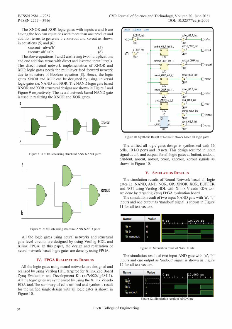
E-ISSN 2581 – 7957 CVR Journal of Science and Technology, Volume 20, June 2021 P-ISSN 2277 – 3916 DOI: 10.32377/cvrjst2009
CVR College of Engineering
The XNOR and XOR logic gates with inputs a and b are having the boolean equations with more than one product and addition terms to generate the xnorout and xorout as shown in equations (5) and (6).
xnorout= ab+a’b’ (5) xorout= ab’+a’b (6)
The above equations 1 and 2 are having two multiplications and one addition terms with direct and inverted input literals. The direct neural network implementation of XNOR and XOR logic gates needs the multilayer feed forward network due to its nature of Boolean equation [8]. Hence, the logic gates XNOR and XOR can be designed by using universal logic gates i.e. NAND and NOR. The NAND logic gate based XNOR and XOR structural designs are shown in Figure 8 and Figure 9 respectively. The neural network based NAND gate is used in realizing the XNOR and XOR gates.
Figure 8. XNOR Gate using structural ANN NAND gates
Figure 9. XOR Gate using structural ANN NAND gates
All the logic gates using neural networks and structural gate level circuits are designed by using Verilog HDL and Xilinx FPGA. In this paper, the design and realization of neural network-based logic gates are done by using FPGA.
. FPGA REALIZATION RESULTS
All the logic gates using neural networks are designed and realized by using Verilog HDL targeted for Xilinx Zed Board Zynq Evaluation and Development Kit (xc7z020clg484-1). All the logic gates are synthesized by using the Xilinx Vivado EDA tool.The summary of cells utilized and synthesis result for the unified single design with all logic gates is shown in Figure 10.
Figure 10. Synthesis Result of Neural Network based all logic gates
The unified all logic gates design is synthesized with 16 cells, 10 I/O ports and 19 nets. This design resulted in input signal as a, b and outputs for all logic gates as bufout, andout, nandout, norout, notout, orout, xnorout, xorout signals as shown in Figure 10.
. SIMULATION RESULTS
The simulation results of Neural Network based all logic gates i.e. NAND, AND, NOR, OR, XNOR, XOR, BUFFER and NOT using Verilog HDL with Xilinx Vivado EDA tool are done by targeting Zynq FPGA evaluation board.
The simulation result of two input NAND gate with ‘a’, ‘b’ inputs and one output as ‘nandout’ signal is shown in Figure 11 for all test vectors.
Figure 11. Simulation result of NAND Gate
The simulation result of two input AND gate with ‘a’, ‘b’ inputs and one output as ‘andout’ signal is shown in Figure 12 for all test vectors.
Figure 12. Simulation result of AND Gate
E-ISSN 2581 – 7957 CVR Journal of Science and Technology, Volume 20, June 2021 P-ISSN 2277 – 3916 DOI: 10.32377/cvrjst2009
CVR College of Engineering
The simulation result of two input NOR gate with ‘a’, ‘b’ inputs and one output as ‘norout’ signal is shown in Figure 13 for all test vectors.
Figure 13. Simulation result of NOR Gate
The simulation result of two input OR gate with ‘a’, ‘b’ inputs and one output as ‘orout’ signal is shown in Figure 14 for all test vectors.
Figure 14. Simulation result of OR Gate
The simulation result of two input XNOR gate with ‘a’, ‘b’ inputs and one output as ‘xnorout’ signal is shown in Figure 15 for all test vectors.
Figure 15. Simulation result of XNOR Gate
The simulation result of two input XOR gate with ‘a’, ‘b’ inputs and one output as ‘xorout’ signal is shown in Figure 16 for all test vectors.
Figure 16. Simulation result of XOR Gate
The simulation result of NOT gate with ‘a’ as input and ‘notout’ as output signal is shown in Figure 17 for all test vectors.
Figure 17. Simulation result of NOT Gate
The simulation result of BUFFER with ‘b’ as input and ‘bufout’ as output signal is shown in Figure 18 for all test vectors.
Figure 18. Simulation result of Buffer
The simulation result of unified structure for Neural Network based all logic gate with ‘a’, ‘b’ as inputs and ‘nandout’, ‘andout’, ‘norout’, ‘orout’, ‘xnorout’, ‘xorout’, ‘notout’, ‘bufout’ is shown in Figure 19 for all test vectors.
Figure 19. Simulation result of all logic gates
. CONCLUSIONS
All the logic gates are realized by using Verilog HDL with Xilinx Vivado Design suite targeting for Xilinx Zynq-7000 SoC Evaluation Board.
The logic gates NAND, AND, NOR, OR, NOT, BUFFER are realized by using single layer neural network with computational equations using Verilog HDL. The XNOR and XOR logic gates are realized by using structural representation of neural network based universal NAND gates. All these logic gates are simulated for different test cases.
A unified structure for Neural Network based all logic gates is designed and synthesized using Xilinx Vivado EDA tool. This unified logic gate structure is simulated for different test cases.

E-ISSN 2581 – 7957 CVR Journal of Science and Technology, Volume 20, June 2021 P-ISSN 2277 – 3916 DOI: 10.32377/cvrjst2009
CVR College of Engineering
[1]. O. I. Abiodun et al., "Comprehensive Review of Artificial Neural Network Applications to Pattern Recognition," in IEEE Access, vol. 7, pp. 158820-158846, 2019.
[2]. Haitham Kareem Ali and Esraa Zeki Mohammed, “ Design Artificial Neural Network Using FPGA”, IJCSNS International Journal of Computer Science and Network Security, Vol.10, No.8, August 2010.
[3]. Ganesh.R, “Design Procedure for Digital and Analog ICs using Cadence Tools”, CVR Journal of Science and Technology, Volume 9, December 2015.
[4]. A. Muthuramalingam, S. Himavathi, E. Srinivasan, “ Neural Network Implementation Using FPGA: Issues and Application”, International Journal of Information Technology, Vol. 4 Issue 2, p86, 2008.
[5]. Murat H. Sazli, “A Brief Review Of Feed-Forward Neural Networks”, Commun. Fac. Sci. Univ. Ank. Series A2-A3, V.50(1), pp 11-17 (2006).
[6]. Crescenzio Gallo, “Artificial Neural Networks Tutorial”, January 2015.
[7]. F. Rosenblatt, “The perceptron: a probabilistic model for Information storage and organization in the brain”, Psychological Review, Vol. 65, No. 6, 1958.
[8]. Blount, D., Banda, P., Teuscher, C., & Stefanovic, D. (2017), “Feedforward Chemical Neural Network: An In Silico Chemical System That Learns XOR. Artificial Life”, Volume 23, Issue 3, p. 295-317.
REFERENCES
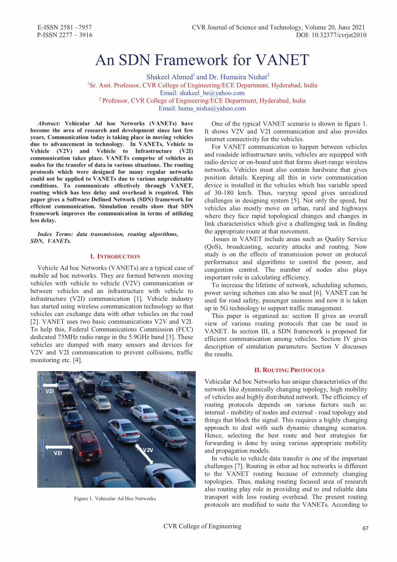
E-ISSN 2581 –7957 CVR Journal of Science and Technology, Volume 20, June 2021 P-ISSN 2277 – 3916 DOI: 10.32377/cvrjst2010
CVR College of Engineering
An SDN Framework for VANET 1Sr. Asst. Professor, CVR College of Engineering/ECE Department, Hyderabad, India
Email: [email protected] 2 Professor, CVR College of Engineering/ECE Department, Hyderabad, India
Email: [email protected]
Abstract: Vehicular Ad hoc Networks (VANETs) have become the area of research and development since last few years. Communication today is taking place in moving vehicles due to advancement in technology. In VANETs, Vehicle to Vehicle (V2V) and Vehicle to Infrastructure (V2I) communication takes place. VANETs comprise of vehicles as nodes for the transfer of data in various situations. The routing protocols which were designed for many regular networks could not be applied to VANETs due to various unpredictable conditions. To communicate effectively through VANET, routing which has less delay and overhead is required. This paper gives a Software Defined Network (SDN) framework for efficient communication. Simulation results show that SDN framework improves the communication in terms of utilizing less delay.
Index Terms: data transmission, routing algorithms, SDN, VANETs.
I. INTRODUCTION
Vehicle Ad hoc Networks (VANETs) are a typical case of mobile ad hoc networks. They are formed between moving vehicles with vehicle to vehicle (V2V) communication or between vehicles and an infrastructure with vehicle to infrastructure (V2I) communication [1]. Vehicle industry has started using wireless communication technology so that vehicles can exchange data with other vehicles on the road [2]. VANET uses two basic communications V2V and V2I. To help this, Federal Communications Commission (FCC) dedicated 75MHz radio range in the 5.9GHz band [3]. These vehicles are dumped with many sensors and devices for V2V and V2I communication to prevent collisions, traffic monitoring etc. [4].
Figure 1. Vehicular Ad Hoc Networks
One of the typical VANET scenario is shown in figure 1. It shows V2V and V2I communication and also provides internet connectivity for the vehicles.
For VANET communication to happen between vehicles and roadside infrastructure units, vehicles are equipped with radio device or on-board unit that forms short-range wireless networks. Vehicles must also contain hardware that gives position details. Keeping all this in view communication device is installed in the vehicles which has variable speed of 30-180 km/h. Thus, varying speed gives unrealized challenges in designing system [5]. Not only the speed, but vehicles also mostly move on urban, rural and highways where they face rapid topological changes and changes in link characteristics which give a challenging task in finding the appropriate route at that movement.
.Issues in VANET include areas such as Quality Service (QoS), broadcasting, security attacks and routing. Now study is on the effects of transmission power on protocol performance and algorithms to control the power, and congestion control. The number of nodes also plays important role in calculating efficiency.
To increase the lifetime of network, scheduling schemes, power saving schemes can also be used [6]. VANET can be used for road safety, passenger easiness and now it is taken up in 5G technology to support traffic management.
This paper is organized as: section II gives an overall view of various routing protocols that can be used in VANET. In section III, a SDN framework is proposed for efficient communication among vehicles. Section IV gives description of simulation parameters. Section V discusses the results.
II. ROUTING PROTOCOLS
Vehicular Ad hoc Networks has unique characteristics of the network like dynamically changing topology, high mobility of vehicles and highly distributed network. The efficiency of routing protocols depends on various factors such as: internal - mobility of nodes and external - road topology and things that block the signal. This requires a highly changing approach to deal with such dynamic changing scenarios. Hence, selecting the best route and best strategies for forwarding is done by using various appropriate mobility and propagation models.
In vehicle to vehicle data transfer is one of the important challenges [7]. Routing in other ad hoc networks is different to the VANET routing because of extremely changing topologies. Thus, making routing focused area of research also routing play role in providing end to end reliable data transport with less routing overhead. The present routing protocols are modified to suite the VANETs. According to
Shakeel Ahmed1 and Dr. Humaira Nishat2
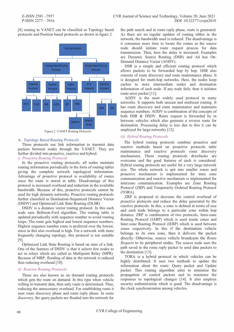
E-ISSN 2581 –7957 CVR Journal of Science and Technology, Volume 20, June 2021 P-ISSN 2277 – 3916 DOI: 10.32377/cvrjst2010
CVR College of Engineering
[8] routing in VANET can be classified as Topology based protocols and Position based protocols as shown in figure 2.
Figure 2. VANET Routing Protocols
A. Topology Based Routing Protocols These protocols use link information to transmit data
packets between nodes through the VANET. They are further divided into proactive, reactive and hybrid. i) Proactive Routing Protocols
In the proactive routing protocols, all nodes maintain routing information periodically in the form of routing tables giving the complete network topological information. Advantage of proactive protocol is availability of routes since the route is stored in table. Disadvantage of this protocol is increased overhead and reduction in the available bandwidth. Because of this, proactive protocols cannot be used for high dynamic networks. Proactive routing protocols further classified as Destination-Sequenced Distance Vector (DSDV) and Optimized Link State Routing (OLSR)
DSDV is a distance vector routing protocol. In this each node uses Bellmon-Ford algorithm. The routing table is updated periodically with sequence number to avoid routing loops. The route gets highest and lowest sequence numbers. Highest sequence number route is preferred over the lowest, since in this also overhead is high. For a network with more frequently changing topology, this protocol is not suitable [9].
Optimized Link State Routing is based on state of a link. One of the features of DSDV is that it selects few nodes to act as relays which are called as Multipoint Relay (MPR). Because of MRP, flooding of data in the network is reduced thus reducing overhead [10].
ii) Reactive Routing ProtocolsThese are also known as on demand routing protocols
which gets the route on demand. In this type when vehicle willing to transmit data, then only route is determined. Thus, reducing the unnecessary overhead. For establishing route it uses route discovery phase and route reply phase. In route discovery, the query packets are flooded into the network for
the path search and in route reply phase, route is generated. As there are no regular updates of routing tables in the network, the bandwidth used is reduced. The disadvantage is it consumes more time to locate the routes as the source node should initiate route request process for data transmission. Thus, here the delay is increased. Examples are Dynamic Source Routing (DSR) and Ad hoc On-Demand Distance Vector (AODV).
DSR is a simple and efficient routing protocol which allows packets to be forwarded hop by hop. DSR also consists of route discovery and route maintenance phase. It is designed for mutti-hop networks. Here, the nodes keep caches to store intermediate nodes and destination information of each node. If any node fails, then it initiates route error packet [11].
AODV is the most widely used protocol in many networks. It supports both unicast and multicast routing. It has route discovery and route maintenance and maintains sequence numbers. AODV is combination of the concepts of both DSR & DSDV. Route request is forwarded by in between vehicles which also generate a reverse route for destination. Processing delay is less due to this it can be employed for large networks [12].
iii) Hybrid Routing ProtocolsThe hybrid routing protocols combine proactive and
reactive methods based on proactive protocols table maintenance and reactive protocols route discovery mechanisms. These routing protocols drawbacks are overcome and the good features of each is considered. Hybrid routing protocols are useful for a very large network size. The whole network is spit into smaller zones and proactive mechanism is implemented for intra zone communication and reactive mechanism is implemented for interzone communication. Examples are Zone Routing Protocol (ZRP) and Temporarily Ordered Routing Protocol (TORA)
ZRP is proposed to decrease the control overhead of proactive protocols and reduce the delay generated by the reactive protocols. In this, a zone is defined in terms of size and each node belongs to a particular zone within hop distance. ZRP is combination of two protocols, Intra-zone Routing Protocol (IARP) which is used inside zones and Inter-zone Routing Protocol (IERP) which is used between zones respectively. In this if the destination vehicle belongs to its own zone, then it delivers the packet directly. Otherwise, source vehicle broadcasts the Route Request to its peripheral nodes. The source node uses the path saved in the route reply packet to send data packets to the destination [13].
TORA is a hybrid protocol in which vehicles can be highly distributed. It uses two methods to update the information about the route: Query packet and Update packet. This routing algorithm aims to minimize the propagation of control packets and to minimize the responses to topological changes [14]. It also employs security authentication which is good. The disadvantage is the clock synchronization among vehicles.
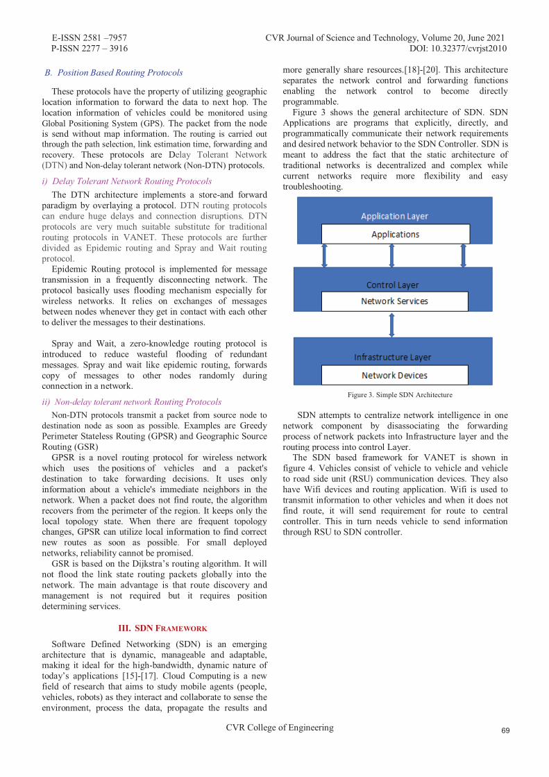
E-ISSN 2581 –7957 CVR Journal of Science and Technology, Volume 20, June 2021 P-ISSN 2277 – 3916 DOI: 10.32377/cvrjst2010
CVR College of Engineering
These protocols have the property of utilizing geographic location information to forward the data to next hop. The location information of vehicles could be monitored using Global Positioning System (GPS). The packet from the node is send without map information. The routing is carried out through the path selection, link estimation time, forwarding and recovery. These protocols are Delay Tolerant Network (DTN) and Non-delay tolerant network (Non-DTN) protocols.
i) Delay Tolerant Network Routing ProtocolsThe DTN architecture implements a store-and forward
paradigm by overlaying a protocol. DTN routing protocols can endure huge delays and connection disruptions. DTN protocols are very much suitable substitute for traditional routing protocols in VANET. These protocols are further divided as Epidemic routing and Spray and Wait routing protocol.
Epidemic Routing protocol is implemented for message transmission in a frequently disconnecting network. The protocol basically uses flooding mechanism especially for wireless networks. It relies on exchanges of messages between nodes whenever they get in contact with each other to deliver the messages to their destinations.
Spray and Wait, a zero-knowledge routing protocol is introduced to reduce wasteful flooding of redundant messages. Spray and wait like epidemic routing, forwards copy of messages to other nodes randomly during connection in a network.
ii) Non-delay tolerant network Routing ProtocolsNon-DTN protocols transmit a packet from source node to
destination node as soon as possible. Examples are Greedy Perimeter Stateless Routing (GPSR) and Geographic Source Routing (GSR)
GPSR is a novel routing protocol for wireless network which uses the positions of vehicles and a packet's destination to take forwarding decisions. It uses only information about a vehicle's immediate neighbors in the network. When a packet does not find route, the algorithm recovers from the perimeter of the region. It keeps only the local topology state. When there are frequent topology changes, GPSR can utilize local information to find correct new routes as soon as possible. For small deployed networks, reliability cannot be promised.
GSR is based on the Dijkstra’s routing algorithm. It will not flood the link state routing packets globally into the network. The main advantage is that route discovery and management is not required but it requires position determining services.
III. SDN FRAMEWORK
Software Defined Networking (SDN) is an emerging architecture that is dynamic, manageable and adaptable, making it ideal for the high-bandwidth, dynamic nature of today’s applications [15]-[17]. Cloud Computing is a new field of research that aims to study mobile agents (people, vehicles, robots) as they interact and collaborate to sense the environment, process the data, propagate the results and
more generally share resources.[18]-[20]. This architecture separates the network control and forwarding functions enabling the network control to become directly programmable.
Figure 3 shows the general architecture of SDN. SDN Applications are programs that explicitly, directly, and programmatically communicate their network requirements and desired network behavior to the SDN Controller. SDN is meant to address the fact that the static architecture of traditional networks is decentralized and complex while current networks require more flexibility and easy troubleshooting.
Figure 3. Simple SDN Architecture
SDN attempts to centralize network intelligence in one network component by disassociating the forwarding process of network packets into Infrastructure layer and the routing process into control Layer.
The SDN based framework for VANET is shown in figure 4. Vehicles consist of vehicle to vehicle and vehicle to road side unit (RSU) communication devices. They also have Wifi devices and routing application. Wifi is used to transmit information to other vehicles and when it does not find route, it will send requirement for route to central controller. This in turn needs vehicle to send information through RSU to SDN controller.
B. Position Based Routing Protocols
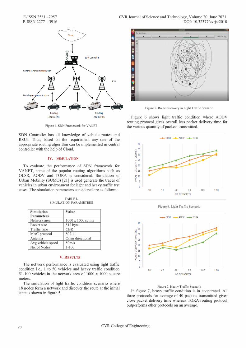
E-ISSN 2581 –7957 CVR Journal of Science and Technology, Volume 20, June 2021 P-ISSN 2277 – 3916 DOI: 10.32377/cvrjst2010
CVR College of Engineering
Figure 4. SDN Framework for VANET
SDN Controller has all knowledge of vehicle routes and RSUs. Thus, based on the requirement any one of the appropriate routing algorithm can be implemented in central controller with the help of Cloud.
To evaluate the performance of SDN framework for VANET, some of the popular routing algorithms such as OLSR, AODV and TORA is considered. Simulation of Urban Mobility (SUMO) [21] is used generate the traces of vehicles in urban environment for light and heavy traffic test cases. The simulation parameters considered are as follows:
TABLE I. SIMULATION PARAMETERS
Simulation Parameters
Value
Network area 1000 x 1000 sqmts Packet size 512 byte Traffic type CBR MAC protocol 802.11 Antenna Omni directional Avg vehicle speed 50m/s No. of Nodes 1-100
The network performance is evaluated using light traffic condition i.e., 1 to 50 vehicles and heavy traffic condition 51-100 vehicles in the network area of 1000 x 1000 square meters.
The simulation of light traffic condition scenario where 18 nodes form a network and discover the route at the initial state is shown in figure 5.
Figure 5. Route discovery in Light Traffic Scenario
Figure 6 shows light traffic condition where AODV routing protocol gives overall less packet delivery time for the various quantity of packets transmitted.
Figure 6. Light Traffic Scenario
Figure 7. Heavy Traffic Scenario In figure 7, heavy traffic condition is in cooperated. All
three protocols for average of 40 packets transmitted gives close packet delivery time whereas TORA routing protocol outperforms other protocols on an average.
V. RESULTS
I . SIMULATION

E-ISSN 2581 –7957 CVR Journal of Science and Technology, Volume 20, June 2021 P-ISSN 2277 – 3916 DOI: 10.32377/cvrjst2010
CVR College of Engineering
V . CONCLUSIONS
There is a demand now for efficient communication in VANET. This paper gives a SDN framework required for dynamic changing feature of VANET. Some of the standard protocols such as OLSR, AODV and TORA are compared in light and heavy traffic conditions in a limited area. It is concluded that in light traffic condition AODV on an average performs better and TORA protocol give better results that is less packet delivery time in high traffic conditions. In future, the protocols with security will be simulated and the various QoS metric will be evaluated.
REFERENCES [1] Y. Toor, P. Muhlethaler, A. Laouiti, and A. D. L. Fortelle,
“Vehicle ad hoc networks: applications and related technical issues,” IEEE Communications Surveys Tutorials, vol. 10, no. 3, pp. 74–88, 2008.
[2] H. Hartenstein and L. P. Laberteaux, “A tutorial survey on vehicular ad hoc networks,” IEEE Communications Magazine, vol. 46, no. 6, pp. 164–171, June 2008
[3] J. Choi, V. Marojevic, R. Nealy, J. H. Reed, and C. B. Dietrich, ‘‘DSRC and IEEE 802.11ac adjacent channel interference assessment for the5.9 GHz band,’’ in Proc. IEEE 89th Veh. Technol. Conf. (VTC-Spring), Kuala Lumpur, Malaysia, Apr. 2019, pp.1-5
[4] Wenshuang Liang, Zhuorong Li, Hongyang Zhang, Shenling Wang, and Rongfang Bie, “Vehicular Ad Hoc Networks: Architectures, Research Issues, Methodologies, Challenges, and Trends”, International Journal of Distributed Sensor Networks, 2015.
[5] S. Zeadally, R. Hunt, Y. S. Chen, A. 1. and A. Hassan, "Vehicular ad hoc networks (VANETS): status, results, and challenges",Springer Science and Business Media, LLC 2010, pp. 217 -241.
[6] Nyoman Wira Prasetya; Tsang-Ling Sheu; Achmad Basuki; Muhammad Aziz Muslim, “A Pre-Emptive Traffic Model with Cluster-based TDMA for Vehicular Networks”, IEEE International Conference on Software, Telecommunications and Computer Networks (SoftCOM), Sep. 2016, pp. 1-5.
[7] E.Royer and C.-K. Toh, "A Review of Current Routing Protocols for Ad Hoc Mobile Wireless Networks", IEEE Personal Communications Magazine, Vol.6, No. 2, April 1999.
[8] Ramandeep Kaur & Chandan Sharma,”Review paper on performance analysis of AODV, DSDV, OLSR on the basis of packet delivery”,IOSR Journal of Computer Engineering (IOSR-JCE) ,Volume 11, Issue 1 (May. -Jun. 2013), e-ISSN: 2278-0661, p- ISSN: 2278-8727
[9] Y. Fengjie, Y.Hui and Z.Ying,” Research on DSDV routing protocol based on wireless mesh network”, Chinese Control And Decision Conference, Shenyang, China, pp. 4292-4297, 2018.
[10] F. De Rango, M. Fotino and S. Marano, "EE-OLSR: Energy Efficient OLSR routing protocol for Mobile ad-hoc Networks," MILCOM 2008 - 2008 IEEE Military Communications Conference, San Diego, CA, USA, 2008, pp. 1-7, doi: 10.1109/MILCOM.2008.4753611.
[11] Mina Vajed Khiavi, Shahram Jamali & Sajjad Jahanbakhsh Gudakahriz,” Performance Comparison of AODV, DSDV, DSR and TORA Routing Protocols in MANETs “International Research Journal of Applied and Basic Sciences, Vol. 3(7), 1429-1436, 2012, ISSN 2251-838X
[12] Charles E. Perkins and Elizabeth M. Royer, "Ad hoc On-Demand Distance Vector Routing", Proceedings of the 2nd
IEEE Workshop on Mobile Computing Systems and Applications (WMCSA ' 99), pp. 90-100, February 1999.
[13] K. Yang and W. Huang, "Performance Research of an Improved Hybrid Routing Protocol," 2019 IEEE 19th International Conference on Communication Technology (ICCT), Xi'an, China, 2019, pp. 1242-1247
[14] Fang Yu, Yun Li, Fei Fang and Qianbin Chen, "A New TORA-based Energy Aware Routing Protocol in Mobile Ad Hoc Networks," 2007 3rd IEEE/IFIP International Conference in Central Asia on Internet, Tashkent, Uzbekistan, 2007, pp. 1-4, doi: 10.1109/CANET.2007.4401666.
[15] S. Bera, S. Misra, and A. V. Vasilakos, “Software-defined networking for internet of things: A survey,” IEEE Internet of Things Journal, vol. 4, no. 6, pp. 1994–2008, 2017.
[16] D. Kreutz, F. M. V. Ramos, P. E. Verssimo, C. E. Rothenberg, S. Azodolmolky, and S. Uhlig, “Software-defined networking: A comprehensive survey,” Proceedings of the IEEE, vol. 103, no. 1, pp. 14–76, Jan 2015.
[17] C. E. Palazzi, M. Roccetti, and S. Ferretti, “An intervehicular communication architecture for safety and entertainment,” IEEE Transactions on Intelligent Transportation Systems, vol. 11, no. 1, pp. 90–99, March 2010.
[18] M. A. Salahuddin, A. Al-Fuqaha, and M. Guizani, “Software-networking for RSU clouds in support of the Internet of vehicles,'' IEEE Internet Things J., vol. 2, no. 2, pp. 133_144, Apr. 2015.
[19] Park SC, Ryoo SY. An empirical investigation of end-users’ switching toward cloud computing: A two factor theory perspective. Computers in Human Behavior 2013; 29(1):160–70.
[20] R. Gasmi and M. Aliouat, "Vehicular Ad Hoc NETworks versus Internet of Vehicles - A Comparative View," 2019 International Conference on Networking and Advanced Systems (ICNAS), Annaba, Algeria, pp. 1-6, 2019
[21] Simulation of Urban Mobility (SUMO). http://sumo-sim.org.
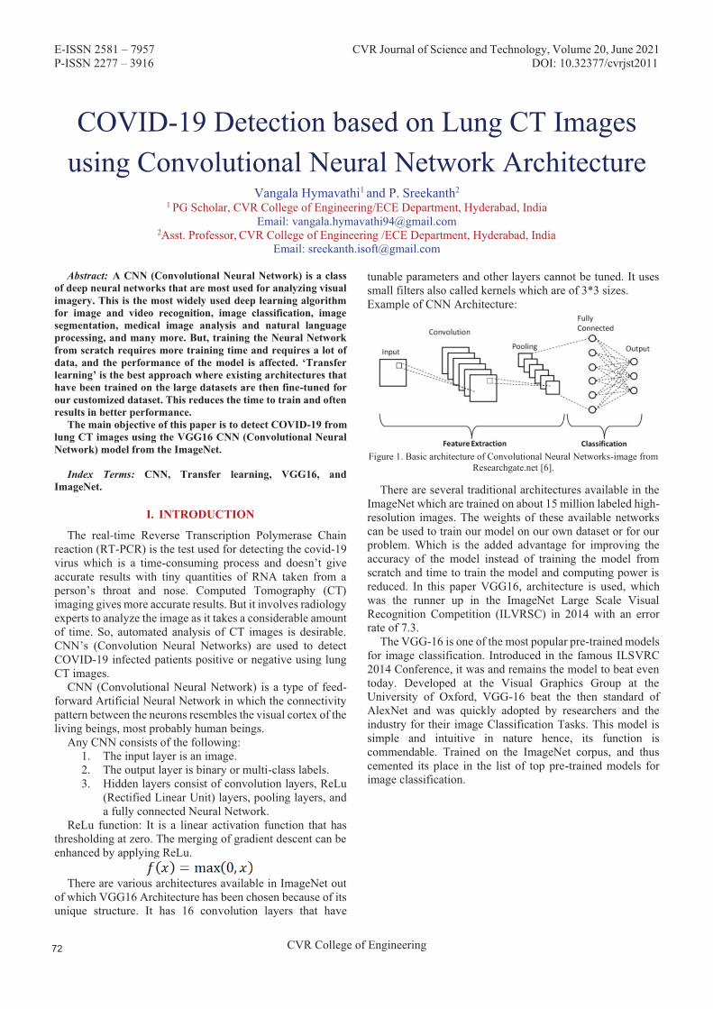
E-ISSN 2581 – 7957 CVR Journal of Science and Technology, Volume 20, June 2021 P-ISSN 2277 – 3916 DOI: 10.32377/cvrjst2011
CVR College of Engineering
COVID-19 Detection based on Lung CT Images using Convolutional Neural Network Architecture
Vangala Hymavathi1 and P. Sreekanth2
Email: [email protected] 2Asst. Professor, CVR College of Engineering /ECE Department, Hyderabad, India
Email: [email protected]
Abstract: A CNN (Convolutional Neural Network) is a class of deep neural networks that are most used for analyzing visual imagery. This is the most widely used deep learning algorithm for image and video recognition, image classification, image segmentation, medical image analysis and natural language processing, and many more. But, training the Neural Network from scratch requires more training time and requires a lot of data, and the performance of the model is affected. ‘Transfer learning’ is the best approach where existing architectures that have been trained on the large datasets are then fine-tuned for our customized dataset. This reduces the time to train and often results in better performance.
The main objective of this paper is to detect COVID-19 from lung CT images using the VGG16 CNN (Convolutional Neural Network) model from the ImageNet.
Index Terms: CNN, Transfer learning, VGG16, and ImageNet.
I. INTRODUCTION
The real-time Reverse Transcription Polymerase Chain reaction (RT-PCR) is the test used for detecting the covid-19 virus which is a time-consuming process and doesn’t give accurate results with tiny quantities of RNA taken from a person’s throat and nose. Computed Tomography (CT) imaging gives more accurate results. But it involves radiology experts to analyze the image as it takes a considerable amount of time. So, automated analysis of CT images is desirable. CNN’s (Convolution Neural Networks) are used to detect COVID-19 infected patients positive or negative using lung CT images.
CNN (Convolutional Neural Network) is a type of feed-forward Artificial Neural Network in which the connectivity pattern between the neurons resembles the visual cortex of the living beings, most probably human beings.
Any CNN consists of the following: 1. The input layer is an image.2. The output layer is binary or multi-class labels.3. Hidden layers consist of convolution layers, ReLu
(Rectified Linear Unit) layers, pooling layers, anda fully connected Neural Network.
ReLu function: It is a linear activation function that has thresholding at zero. The merging of gradient descent can be enhanced by applying ReLu.
There are various architectures available in ImageNet out of which VGG16 Architecture has been chosen because of its unique structure. It has 16 convolution layers that have
tunable parameters and other layers cannot be tuned. It uses small filters also called kernels which are of 3*3 sizes. Example of CNN Architecture:
Figure 1. Basic architecture of Convolutional Neural Networks-image from Researchgate.net [6].
There are several traditional architectures available in the ImageNet which are trained on about 15 million labeled high-resolution images. The weights of these available networks can be used to train our model on our own dataset or for our problem. Which is the added advantage for improving the accuracy of the model instead of training the model from scratch and time to train the model and computing power is reduced. In this paper VGG16, architecture is used, which was the runner up in the ImageNet Large Scale Visual Recognition Competition (ILVRSC) in 2014 with an error rate of 7.3.
The VGG-16 is one of the most popular pre-trained models for image classification. Introduced in the famous ILSVRC 2014 Conference, it was and remains the model to beat even today. Developed at the Visual Graphics Group at the University of Oxford, VGG-16 beat the then standard of AlexNet and was quickly adopted by researchers and the industry for their image Classification Tasks. This model is simple and intuitive in nature hence, its function is commendable. Trained on the ImageNet corpus, and thus cemented its place in the list of top pre-trained models for image classification.
g
1 PG Scholar, CVR College of Engineering/ECE Department, Hyderabad, India
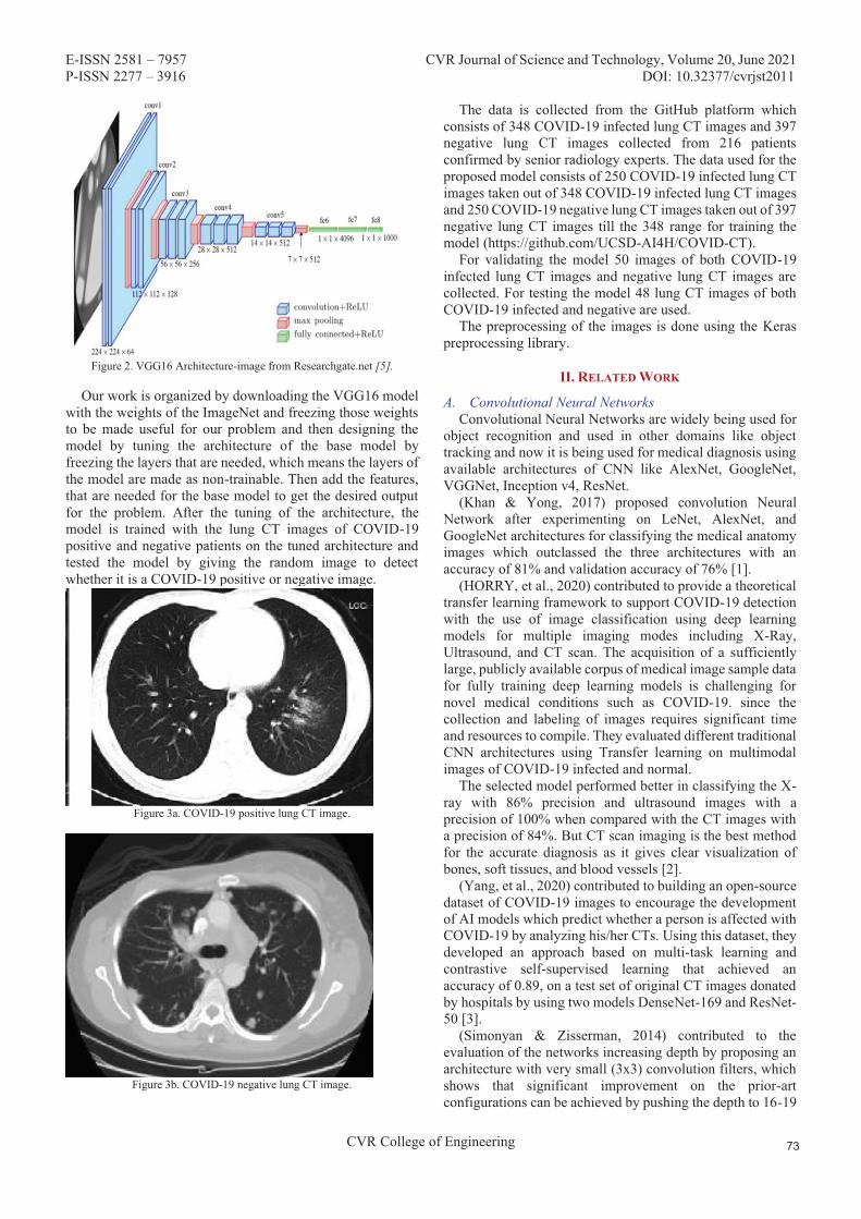
E-ISSN 2581 – 7957 CVR Journal of Science and Technology, Volume 20, June 2021 P-ISSN 2277 – 3916 DOI: 10.32377/cvrjst2011
CVR College of Engineering
Figure 2. VGG16 Architecture-image from Researchgate.net [5].
Our work is organized by downloading the VGG16 model with the weights of the ImageNet and freezing those weights to be made useful for our problem and then designing the model by tuning the architecture of the base model by freezing the layers that are needed, which means the layers of the model are made as non-trainable. Then add the features, that are needed for the base model to get the desired output for the problem. After the tuning of the architecture, the model is trained with the lung CT images of COVID-19 positive and negative patients on the tuned architecture and tested the model by giving the random image to detect whether it is a COVID-19 positive or negative image.
Figure 3a. COVID-19 positive lung CT image.
Figure 3b. COVID-19 negative lung CT image.
The data is collected from the GitHub platform which consists of 348 COVID-19 infected lung CT images and 397 negative lung CT images collected from 216 patients confirmed by senior radiology experts. The data used for the proposed model consists of 250 COVID-19 infected lung CT images taken out of 348 COVID-19 infected lung CT images and 250 COVID-19 negative lung CT images taken out of 397 negative lung CT images till the 348 range for training the model (https://github.com/UCSD-AI4H/COVID-CT).
For validating the model 50 images of both COVID-19 infected lung CT images and negative lung CT images are collected. For testing the model 48 lung CT images of both COVID-19 infected and negative are used.
The preprocessing of the images is done using the Keras preprocessing library.
II. RELATED WORK
A. Convolutional Neural Networks Convolutional Neural Networks are widely being used for
object recognition and used in other domains like object tracking and now it is being used for medical diagnosis using available architectures of CNN like AlexNet, GoogleNet, VGGNet, Inception v4, ResNet.
(Khan & Yong, 2017) proposed convolution Neural Network after experimenting on LeNet, AlexNet, and GoogleNet architectures for classifying the medical anatomy images which outclassed the three architectures with an accuracy of 81% and validation accuracy of 76% [1].
(HORRY, et al., 2020) contributed to provide a theoretical transfer learning framework to support COVID-19 detection with the use of image classification using deep learning models for multiple imaging modes including X-Ray, Ultrasound, and CT scan. The acquisition of a sufficiently large, publicly available corpus of medical image sample data for fully training deep learning models is challenging for novel medical conditions such as COVID-19. since the collection and labeling of images requires significant time and resources to compile. They evaluated different traditional CNN architectures using Transfer learning on multimodal images of COVID-19 infected and normal.
The selected model performed better in classifying the X-ray with 86% precision and ultrasound images with a precision of 100% when compared with the CT images with a precision of 84%. But CT scan imaging is the best method for the accurate diagnosis as it gives clear visualization of bones, soft tissues, and blood vessels [2].
(Yang, et al., 2020) contributed to building an open-source dataset of COVID-19 images to encourage the development of AI models which predict whether a person is affected with COVID-19 by analyzing his/her CTs. Using this dataset, they developed an approach based on multi-task learning and contrastive self-supervised learning that achieved an accuracy of 0.89, on a test set of original CT images donated by hospitals by using two models DenseNet-169 and ResNet-50 [3].
(Simonyan & Zisserman, 2014) contributed to the evaluation of the networks increasing depth by proposing an architecture with very small (3x3) convolution filters, which shows that significant improvement on the prior-art configurations can be achieved by pushing the depth to 16-19
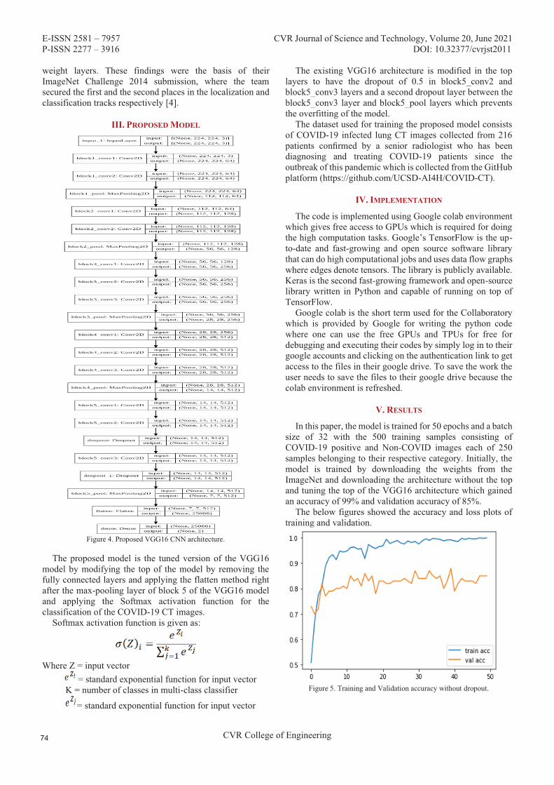
E-ISSN 2581 – 7957 CVR Journal of Science and Technology, Volume 20, June 2021 P-ISSN 2277 – 3916 DOI: 10.32377/cvrjst2011
CVR College of Engineering
weight layers. These findings were the basis of their ImageNet Challenge 2014 submission, where the team secured the first and the second places in the localization and classification tracks respectively [4].
III. PROPOSED MODEL
Figure 4. Proposed VGG16 CNN architecture.
The proposed model is the tuned version of the VGG16 model by modifying the top of the model by removing the fully connected layers and applying the flatten method right after the max-pooling layer of block 5 of the VGG16 model and applying the Softmax activation function for the classification of the COVID-19 CT images.
Softmax activation function is given as:
Where Z = input vector = standard exponential function for input vector
K = number of classes in multi-class classifier
= standard exponential function for input vector
The existing VGG16 architecture is modified in the top layers to have the dropout of 0.5 in block5_conv2 and block5_conv3 layers and a second dropout layer between the block5_conv3 layer and block5_pool layers which prevents the overfitting of the model.
The dataset used for training the proposed model consists of COVID-19 infected lung CT images collected from 216 patients confirmed by a senior radiologist who has been diagnosing and treating COVID-19 patients since the outbreak of this pandemic which is collected from the GitHub platform (https://github.com/UCSD-AI4H/COVID-CT).
IV. IMPLEMENTATION
The code is implemented using Google colab environment which gives free access to GPUs which is required for doing the high computation tasks. Google’s TensorFlow is the up-to-date and fast-growing and open source software library that can do high computational jobs and uses data flow graphs where edges denote tensors. The library is publicly available. Keras is the second fast-growing framework and open-source library written in Python and capable of running on top of TensorFlow.
Google colab is the short term used for the Collaboratory which is provided by Google for writing the python code where one can use the free GPUs and TPUs for free for debugging and executing their codes by simply log in to their google accounts and clicking on the authentication link to get access to the files in their google drive. To save the work the user needs to save the files to their google drive because the colab environment is refreshed.
V. RESULTS
In this paper, the model is trained for 50 epochs and a batch size of 32 with the 500 training samples consisting of COVID-19 positive and Non-COVID images each of 250 samples belonging to their respective category. Initially, the model is trained by downloading the weights from the ImageNet and downloading the architecture without the top and tuning the top of the VGG16 architecture which gained an accuracy of 99% and validation accuracy of 85%.
The below figures showed the accuracy and loss plots of training and validation.
Figure 5. Training and Validation accuracy without dropout.
g
g
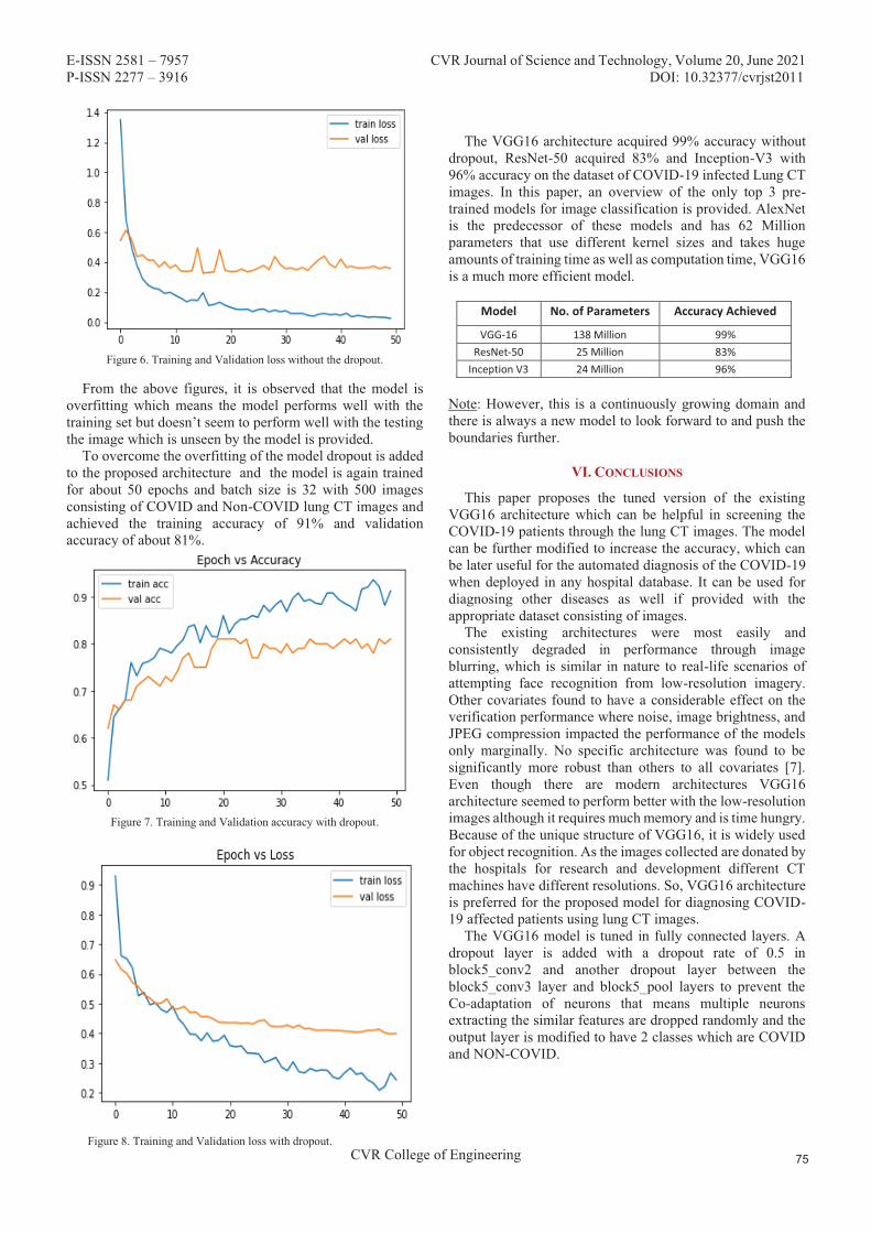
E-ISSN 2581 – 7957 CVR Journal of Science and Technology, Volume 20, June 2021 P-ISSN 2277 – 3916 DOI: 10.32377/cvrjst2011
CVR College of Engineering
Figure 6. Training and Validation loss without the dropout.
From the above figures, it is observed that the model is overfitting which means the model performs well with the training set but doesn’t seem to perform well with the testing the image which is unseen by the model is provided.
To overcome the overfitting of the model dropout is added to the proposed architecture and the model is again trained for about 50 epochs and batch size is 32 with 500 images consisting of COVID and Non-COVID lung CT images and achieved the training accuracy of 91% and validation accuracy of about 81%.
Figure 7. Training and Validation accuracy with dropout.
Figure 8. Training and Validation loss with dropout.
The VGG16 architecture acquired 99% accuracy without dropout, ResNet-50 acquired 83% and Inception-V3 with 96% accuracy on the dataset of COVID-19 infected Lung CT images. In this paper, an overview of the only top 3 pre-trained models for image classification is provided. AlexNet is the predecessor of these models and has 62 Million parameters that use different kernel sizes and takes huge amounts of training time as well as computation time, VGG16 is a much more efficient model.
Model No. of Parameters Accuracy Achieved
VGG-16 138 Million 99% ResNet-50 25 Million 83%
Inception V3 24 Million 96%
Note: However, this is a continuously growing domain and there is always a new model to look forward to and push the boundaries further.
VI. CONCLUSIONS
This paper proposes the tuned version of the existing VGG16 architecture which can be helpful in screening the COVID-19 patients through the lung CT images. The model can be further modified to increase the accuracy, which can be later useful for the automated diagnosis of the COVID-19 when deployed in any hospital database. It can be used for diagnosing other diseases as well if provided with the appropriate dataset consisting of images.
The existing architectures were most easily and consistently degraded in performance through image blurring, which is similar in nature to real-life scenarios of attempting face recognition from low-resolution imagery. Other covariates found to have a considerable effect on the verification performance where noise, image brightness, and JPEG compression impacted the performance of the models only marginally. No specific architecture was found to be significantly more robust than others to all covariates [7]. Even though there are modern architectures VGG16 architecture seemed to perform better with the low-resolution images although it requires much memory and is time hungry. Because of the unique structure of VGG16, it is widely used for object recognition. As the images collected are donated by the hospitals for research and development different CT machines have different resolutions. So, VGG16 architecture is preferred for the proposed model for diagnosing COVID-19 affected patients using lung CT images.
The VGG16 model is tuned in fully connected layers. A dropout layer is added with a dropout rate of 0.5 in block5_conv2 and another dropout layer between the block5_conv3 layer and block5_pool layers to prevent the Co-adaptation of neurons that means multiple neurons extracting the similar features are dropped randomly and the output layer is modified to have 2 classes which are COVID and NON-COVID.

E-ISSN 2581 – 7957 CVR Journal of Science and Technology, Volume 20, June 2021 P-ISSN 2277 – 3916 DOI: 10.32377/cvrjst2011
CVR College of Engineering
[1]. S. Khan and S.-P. Yong, “A deep learning architecture for classifying medical images of anatomy object,” in 2017
[2]. M. J. HORRY, S. CHAKRABORTY, M. PAUL, A. ULHAQ, B. PRADHAN, M. SAHA and N. SHUKLA, “COVID-19 Detection through Transfer Learning using Multimodal Imaging Data,” 2020.
[3]. X. Yang, X. He, J. Zhao, Y. Zhang, S. Zhang and P. Xie, “COVID-CT-Dataset: A CT Scan Dataset about COVID-19,” 2020.
[4]. k. simonyan and A. Zisserman, “Very Deep Convolutional Networks for Large-Scale Image Recognition,” 2014.
[5]. M. Ferguson, “Automatic localization of casting defects with convolutional neural networks,” IEEE International Conference on Big Data (Big Data) At Boston, MA, USA, December 2017.
[6]. V. H. Phung and E. J. Rhee, “A High-Accuracy Model Average Ensemble of Convolutional Neural Networks for Classification of Cloud Image Patches on Small Datasets,” no. Machine Learning Techniques Applied to Geospatial Big Data, 2019.
[7]. Grm, K., Štruc, V., Artiges, A., Caron, M., & Ekenel, H. K. (2018). Strengths and weaknesses of deep learning models for face recognition against image degradations. (pp. 81-89). IET Biometrics.
REFERENCES

E-ISSN 2581 – 7957 CVR Journal of Science and Technology, Volume 20, June 2021 P-ISSN 2277 – 3916 DOI: 10.32377/cvrjst2012
CVR College of Engineering
Power Electronic Circuits and Control Strategies for Improving the Performance of EVs & HEVs
Dr. G. Sree Lakshmi1 and G. Divya2 1Professor, CVR College of Engineering/ EEE Department, Hyderabad, India
Email: [email protected] 2Asst. Professor, CVR College of Engineering/ EEE Department, Hyderabad, India
Email: [email protected]
Abstract: To give cleaner air to future generation with less pollution and to protect our atmosphere from depletion of ozone layer there is a great need of adaptation of emission free vehicles like EVs and HEVs. Even though Government is giving many incentives and subsidies in making the shift towards EVs and HEVs, but due to lack of storage system, less improvement in power electronics and drive system, there is no prominent increase in the emission free transportation on road. With good storage system the cost of the EVs and HEVs are increasing when compared to ICE vehicles. A huge research is taking place in this area. This paper gives the details of Converters, Inverters and Control strategies used in EVs and HEVs to compare which is best suitable to increase the performance of EVs and HEVs. Basic Conventional Vehicle and Hybrid Vehicle system simulation results are taken, and they are compared to understand the advantages and improving the usage of EVs and HEVs with proper storage system.
Index terms: Electric Vehicle (EV), Hybrid Electric Vehicle (HEV), Internal Combustion Engine (ICE).
I. INTRODUCTION
In order to increase the HEVs performance the power electronic circuit is playing a prominent role. The main important Power electronic circuits in HEVs are Converters and Inverters. Converter is used to increase the voltage levels in EVs whereas the inverter is used to convert AC to DC. In addition to above uses there are many other advantages by using Inverters and Converters. In order to apply the concept for the HEVs it is very important to know which converters and inverters can be used in Electric Vehicles. So, this paper demonstrates the classification of the both converters and inverters used in HEVs. In order to understand the characteristics of Conventional and Hybrid vehicle it is essential to understand all the Inverters and Converters topologies used in to decide which is best. Previous simulation analysis and results have been taken and analyzed. The results show that EVs and HEVs have good advantages than that of Conventional Vehicles. The performance can be further increased by using proper combination of Inverters and Converters topology.
II. CONVERTERS
DC-DC converters are the main converters which are used in HEVs. Converters help to interface connection between battery and any energy storage device to DC-link. As there is need for decrease or increase of voltage level, at least one DC-DC converter is needed. So a high powered DC/DC converter is needed for supplying power for the Electric Vehicles. Power converter range varies from 20kW to 200kW. There are three different types of DC-DC converters. Mostly Bi-directional DC-DC converters are needed as power is made to flow in both the directions [1].
A. Isolated Converters 1. Traditional DC-DC Converters:a) Boost Converter: This type of converter uses only
positive voltage gain which is greater than that isneeded for motor action. So, Boost converter ismostly used in EVs. The polarities are same for inputand output.
Figure 1. Boost Converter
b) Buck-Boost: It is used for increasing and decreasingthe voltage level.
c) Cuk: It is current-Voltage- Current Converter. It isused for increasing and decreasing the voltage level.Mostly used for storing energy.
d) Charge Pump Converter: It is used in low powerapplication and can lower voltage level as well asinversing the level of voltage.
2. Interleaved DC-DC Converter:The main advantage of this type of converter is it can
increase voltage level more than four percent. The current ripple at input side and voltage ripples at output side will be
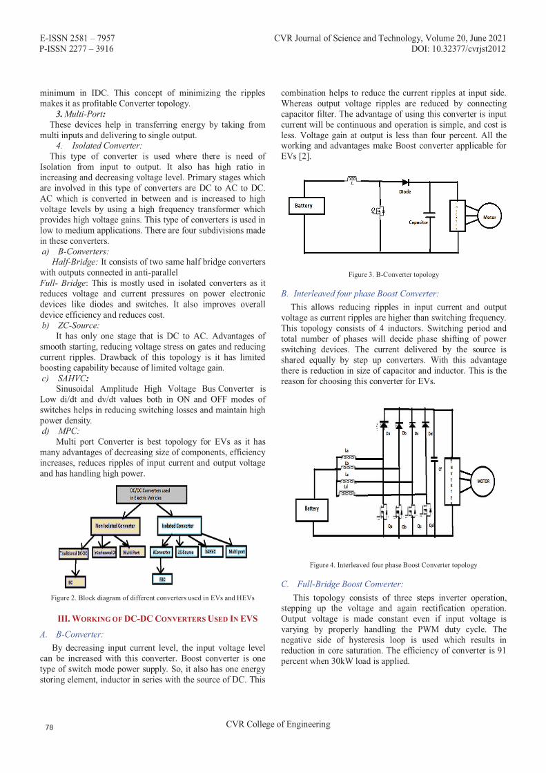
E-ISSN 2581 – 7957 CVR Journal of Science and Technology, Volume 20, June 2021 P-ISSN 2277 – 3916 DOI: 10.32377/cvrjst2012
CVR College of Engineering
minimum in IDC. This concept of minimizing the ripples makes it as profitable Converter topology.
3. Multi-Port:These devices help in transferring energy by taking from
multi inputs and delivering to single output. 4. Isolated Converter:
This type of converter is used where there is need of Isolation from input to output. It also has high ratio in increasing and decreasing voltage level. Primary stages which are involved in this type of converters are DC to AC to DC. AC which is converted in between and is increased to high voltage levels by using a high frequency transformer which provides high voltage gains. This type of converters is used in low to medium applications. There are four subdivisions made in these converters. a) B-Converters:
Half-Bridge: It consists of two same half bridge converters with outputs connected in anti-parallel Full- Bridge: This is mostly used in isolated converters as it reduces voltage and current pressures on power electronic devices like diodes and switches. It also improves overall device efficiency and reduces cost. b) ZC-Source:
It has only one stage that is DC to AC. Advantages ofsmooth starting, reducing voltage stress on gates and reducing current ripples. Drawback of this topology is it has limited boosting capability because of limited voltage gain. c) SAHVC:
Sinusoidal Amplitude High Voltage Bus Converter isLow di/dt and dv/dt values both in ON and OFF modes of switches helps in reducing switching losses and maintain high power density. d) MPC:
Multi port Converter is best topology for EVs as it hasmany advantages of decreasing size of components, efficiency increases, reduces ripples of input current and output voltage and has handling high power.
Figure 2. Block diagram of different converters used in EVs and HEVs
III. WORKING OF DC-DC CONVERTERS USED IN EVS
A. B-Converter: By decreasing input current level, the input voltage level
can be increased with this converter. Boost converter is one type of switch mode power supply. So, it also has one energy storing element, inductor in series with the source of DC. This
combination helps to reduce the current ripples at input side. Whereas output voltage ripples are reduced by connecting capacitor filter. The advantage of using this converter is input current will be continuous and operation is simple, and cost is less. Voltage gain at output is less than four percent. All the working and advantages make Boost converter applicable for EVs [2].
Figure 3. B-Converter topology
B. Interleaved four phase Boost Converter: This allows reducing ripples in input current and output
voltage as current ripples are higher than switching frequency. This topology consists of 4 inductors. Switching period and total number of phases will decide phase shifting of power switching devices. The current delivered by the source is shared equally by step up converters. With this advantage there is reduction in size of capacitor and inductor. This is the reason for choosing this converter for EVs.
Figure 4. Interleaved four phase Boost Converter topology
C. Full-Bridge Boost Converter: This topology consists of three steps inverter operation,
stepping up the voltage and again rectification operation. Output voltage is made constant even if input voltage is varying by properly handling the PWM duty cycle. The negative side of hysteresis loop is used which results in reduction in core saturation. The efficiency of converter is 91 percent when 30kW load is applied.

E-ISSN 2581 – 7957 CVR Journal of Science and Technology, Volume 20, June 2021 P-ISSN 2277 – 3916 DOI: 10.32377/cvrjst2012
CVR College of Engineering
Figure 5. Full-Bridge Boost Converter circuit
D. ZC-Source: By this Converter the efficiency can be increased more than
Full-Bridge Boost Converter, easy to control, light weight and small. With the help of Zero Voltage Switching Converter soft switching and cold starting is possible. The model is like dual half bridge circuitry which is placed on both the sides of transformer. Bi-directional power flow is possible without adding additional devices. Splitting DC Capacitor is needed in order to handle full load current, because stress due to high voltage across power switches in high power applications. ZC-Source also needs large filters to reduce ripples in output voltage.
Figure 6. ZC-Source
IV. INVERTERS USED IN HYBRID VEHICLES
EVs operate with high DC bus voltage and high value of power capacity around 48V to 800V with 10kW to 200kW power capacity. Inverter will change the speed of the motor by rotating frequency. It also controls motor in EVs and determines driving behavior. In addition to above function inverter will capture the energy during regenerative braking as well. So, efficiency of vehicle is determined by the inverter performance [3].
A. Traction Inverter types: 1. Packaged box-type inverter: It has 6-pack which is
filled with six pack gel.2. Integrated inverter design: Small and fully
encapsulated power modules which are placed incompartment of drive train. Electric machines can beintegrated into as fully transmission part byintegrating power inverter in same circuit. This typeof inverter design importance is growing because ofvery attractive features like cooling, vibration, sizeand cost.
3. Multi-level Inverter: The structure of this inverterhelps the vehicle in achieving high voltages to meetthe needs of heavy vehicles. As levels increases theoutput obtained will have number of steps andharmonic wave distortion in the output alsodecreases.
4. Cascaded H-Bridge inverter: This constructionconsists of series of full bridge inverter units in threephases. This unit serves as battery. In this each lowvoltage battery is isolated through switches andleakage current is less when switch is in on condition[4]-[6].
Figure 7. Cascaded H-Bridge inverter circuitry
V. CONTROL STRATEGIES USED IN EVS
Generally, the Hybrid Electric Vehicle requires controlling the drive train. Main aim of any control strategy is to reduce error. Specially in case of meeting the power demand, improving efficiency, State of Charge of battery and storing energy even while applying the brakes. Normally PWM Control is used for DC Motors and Induction Motors use Field Oriented Control (FOC) and Direct Torque Control (DTC).

E-ISSN 2581 – 7957 CVR Journal of Science and Technology, Volume 20, June 2021 P-ISSN 2277 – 3916 DOI: 10.32377/cvrjst2012
CVR College of Engineering
These control strategies are controlled by many different algorithms which are introduced in recent studies. Those control strategies are Classical Control Proportional Integral Derivative (PID), adaptive control, Fuzzy control, Neuro Network control.
A) PID Control:Generally, Inputs for the controller are torque and speed
of the road. The voltage and current are drawn depending on requirement. Here the voltage demanded is compared to voltage which is given as reference. The difference which is obtained by comparing these two is given as error signal to PID controller. Depending on the error signal the voltage is decreased, and the current value is increased depending on the requirement by the HEVs. In HEVs there is problem with electric phase with respect to rising time and settling time. This control strategy will help in managing to which not possible with normal control strategies [8].
Figure 8. PID Control Circuitry
B) Fuzzy Control:In the Fuzzy control only the PID is substituted with the
Fuzzy block and an Integrator and the result obtained after comparison of reference and output is used to decide how much voltage is needed and depending on that voltage level is managed to meet the power demand [7].
Figure 9. Fuzzy Control Circuitry
C) Neural Network Control:The inputs needed for this model are torque, SOC of battery
and speed. There are four different layers in this control they are input layer (m), output layer (n), hidden layer and undertaken layer. Selection of parameters Neural Network Control Strategies is determined by equation :
(1) is the constant value which is approximately equal to from
value 1 to 10. This method is trained by Levenberg-Marquardt algorithm. This method is trained by human brain. With proper training Neural method can produced maximum torque and reduce fuel consumption as well when compared to other methods. Fig 10 shows the neural network model and Fig.11. shows the structure of neural network [9].
Figure 10. Neural Network Model
Figure 11. Structure of Neural Network

E-ISSN 2581 – 7957 CVR Journal of Science and Technology, Volume 20, June 2021 P-ISSN 2277 – 3916 DOI: 10.32377/cvrjst2012
CVR College of Engineering
VI. SIMULATION RESULTS OF HYBRID ELECTRICVEHICLE
Figure 12. Block diagram of Basic Hybrid Electric Vehicle
Figure 13. Simulation results of Hybrid Electric Vehicle of Power vs Vehicle Speed
VII. SIMULATION RESULTS OF CONVENTIONAL V HICLEWITH CITY DRIVE CYCLE
Figure 14. Block diagram of basic Conventional Vehicle with driving cycle
Figure 15. Simulation result of Conventional vehicle of Speed, fuel economy [5]
In the Fig. 12 block diagram of Basic Hybrid Electric Vehicle is shown and in Fig. 13 the power verses vehicle speed characteristics is shown for HEV. In Fig.14 Block diagram of basic conventional vehicle with driving cycle is shown. In Fig.15 simulation results of conventional vehicle of speed fuel economy is shown. From the above two simulations from Fig.13 and Fig.15 which have been taken from two different analysis, it is understood that EVs have a very good Speed Velocity, Battery state of charge and Engine power when compared to Conventional vehicles. In addition to these added features EVs are environmentally friendly. With minimum development in EVs technology the simulation results have shown greater results. So, it is necessary to improve Converter and Inverter part along with other power electronic circuit in order to receive customer acceptance in a large number. Especially in the case of fuel storage and usage of stored fuel where circuits which involve electronic circuit comes into existence.

E-ISSN 2581 – 7957 CVR Journal of Science and Technology, Volume 20, June 2021 P-ISSN 2277 – 3916 DOI: 10.32377/cvrjst2012
CVR College of Engineering
VIII.
The paper has projected on importance of power electronic circuits and control strategies for EVs and HEVs. The basic Inverters, Converters and control strategies introduction are given. Also, simulation results which have been taken show that the HEVs give best results when compared to conventional ICE vehicles. This show if major improvements can be made in drive system and power electronic circuit increases the performance of EVs and HEVs. With increase in performance of emission less electric vehicle more adoption by customers can be gained.
[1] Monzer Al Sakka, Joeri Van Mierlo, and Hamid Gualous, “DC/DC Converters for Electric Vehicles” in In. book: “Electric Vehicles- Modelling and simulation,” Sep-2011, J. Clerk Maxwell, a Treatise on Electricity and Magnetism, 3rd ed., vol.2. Oxford: Clarendon, 1892, pp.68-73.
[2] Sajib Chakraborty 1,2 , Hai-Nam Vu 1,2, Mohammed Mahedi Hasan 1,2, Dai-Duong Tran 1,2 , Mohamed El Baghdadi 1,2 and Omar Hegazy 1,2,*,” DC-DC Converter Topologies for Electric Vehicles, Plug-in Hybrid Electric Vehicles and Fast Charging Stations: State of the Art and Future Trends”, 25 April 2019.K. Elissa.
[3] Leon M. Tolbert, Fang Z. Peng, Thosmas G. Habetler, “Multilevel inverters for Electric Vehicles Application,” WPET-98, Dearborn, Michigan, October 22-23, 1998. Pp-79-84.
[4] Abrar Ahmed,Palasksh Yelamali,R.UdayaKumar,”Modellingand simulation of hybrid technology in vehicles”, The 6th
International Conference on Power and Energy Systems Engineering (CPESE 2019), September 20–23, 2019, Okinawa, Japan”,volume 6 February 2020, Pages 589-594M.
[5] Conventional Vehicle Spark-Ignition Engine Fuel Economy and Emissions”, https://in.mathworks.com/help/autoblks/ug/conventional-vehicle-fuel-economy.html”.
[6] Syed Mohd Harussani Syed Omar, N. M. Arshad, I. M. Yassin, Mohd Hadi Anuar Mohd Fakharuzi, Tom Ward, “ Design andOptimization of a Powertrain systems for a prototype fuel cell electric vehicle,” Pages: 1401-1413, Journal of Mechanical Engineering and Sciences, Vol 8,Published 30 june 2015.
[7] S.k.jha, Anil Kumar Yadav,Prerna Gaur,” Power management for electric vehicle with PID and Fuzzy logic controllers”, 2017 International conference of Electronics, Communication and Aerospace Technology (ICECA),” April 2017 DOI: 10.1109/ICECA.2017.8212731.
[8] Hmidi Mohamed Elhedi, Ines Ben Salem,Lilia El Amaroui,”2DOF PID for dynamic control of drive system hybrid vehicle electrical”.
[9] “Ruijun Liu,1 Dapai Shi,1 and Chao Ma1”,Real-Time Control Strategy of Elman Neural Network for the Parallel Hybrid Electric Vehicle”, Volume 2014 |Article ID 596326 | https://doi.org/10.1155/2014/596326.
CONCLUSIONS
REFERENCES
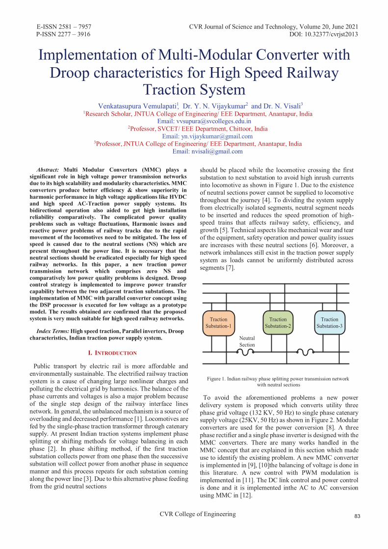
E-ISSN 2581 – 7957 CVR Journal of Science and Technology, Volume 20, June 2021 P-ISSN 2277 – 3916 DOI: 10.32377/cvrjst2013
CVR College of Engineering
Implementation of Multi-Modular Converter with Droop characteristics for High Speed Railway
Traction System Venkatasupura Vemulapati1 Dr. Y N Vijaykumar2 and Dr. N Visali3
1
2Professor, SVCET/ EEE Department, Chittoor, India
3Professor, JNTUA College of Engineering/ EEE Department, Anantapur, India
Abstract: Multi Modular Converters (MMC) plays a significant role in high voltage power transmission networks due to its high scalability and modularity characteristics. MMC converters produce better efficiency & show superiority in harmonic performance in high voltage applications like HVDC and high speed AC-Traction power supply systems. Its bidirectional operation also aided to get high installation reliability comparatively. The complicated power quality problems such as voltage fluctuations, Harmonic issues and reactive power problems of railway tracks due to the rapid movement of the locomotives need to be mitigated. The loss of speed is caused due to the neutral sections (NS) which are present throughout the power line. It is necessary that the neutral sections should be eradicated especially for high speed railway networks. In this paper, a new traction power transmission network which comprises zero NS and comparatively low power quality problems is designed. Droop control strategy is implemented to improve power transfer capability between the two adjacent traction substations. The implementation of MMC with parallel converter concept using the DSP processor is executed for low voltage as a prototype model. The results obtained are confirmed that the proposed system is very much suitable for high speed railway networks.
Index Terms: High speed traction, Parallel inverters, Droop characteristics, Indian traction power supply system.
I. INTRODUCTION
Public transport by electric rail is more affordable and environmentally sustainable. The electrified railway traction system is a cause of changing large nonlinear charges and polluting the electrical grid by harmonics. The balance of the phase currents and voltages is also a major problem because of the single step design of the railway interface lines network. In general, the unbalanced mechanism is a source of overloading and decreased performance [1]. Locomotives are fed by the single-phase traction transformer through catenary supply. At present Indian traction systems implement phase splitting or shifting methods for voltage balancing in each phase [2]. In phase shifting method, if the first traction substation collects power from one phase then the successive substation will collect power from another phase in sequence manner and this process repeats for each substation coming along the power line [3]. Due to this alternative phase feeding from the grid neutral sections
should be placed while the locomotive crossing the first substation to next substation to avoid high inrush currents into locomotive as shown in Figure 1. Due to the existence of neutral sections power cannot be supplied to locomotive throughout the journey [4]. To dividing the system supply from electrically isolated segments, neutral segment needs to be inserted and reduces the speed promotion of high-speed trains that affects railway safety, efficiency, and growth [5]. Technical aspects like mechanical wear and tear of the equipment, safety operation and power quality issues are increases with these neutral sections [6]. Moreover, a network imbalances still exist in the traction power supply system as loads cannot be uniformly distributed across segments [7].
TractionSubstation-1
TractionSubstation-2
TractionSubstation-3
NeutralSection
Figure 1. Indian railway phase splitting power transmission network with neutral sections
To avoid the aforementioned problems a new power delivery system is proposed which converts utility three phase grid voltage (132 KV, 50 Hz) to single phase catenary supply voltage (25KV, 50 Hz) as shown in Figure 2. Modular converters are used for the power conversion [8]. A three phase rectifier and a single phase inverter is designed with the MMC converters. There are many works handled in the MMC concept that are explained in this section which made use to identify the existing problem. A new MMC converter is implemented in [9], [10] the balancing of voltage is done in this literature. A new control with PWM modulation is implemented in [11]. The DC link control and power control is done and it is implemented in the AC to AC conversion using MMC in [12].
Email: [email protected]
Email: [email protected]
Email: [email protected]
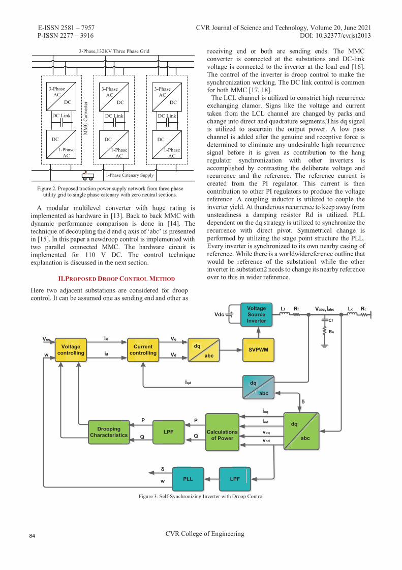
E-ISSN 2581 – 7957 CVR Journal of Science and Technology, Volume 20, June 2021 P-ISSN 2277 – 3916 DOI: 10.32377/cvrjst2013
CVR College of Engineering
3-PhaseAC
DC
1-PhaseAC
DC
DC Link
3-Phase,132KV Three Phase Grid
1-Phase Catenary Supply
3-PhaseAC
DC
1-PhaseAC
DC
DC Link
3-PhaseAC
DC
1-PhaseAC
DC
DC Link
MM
CCo
nver
ter
Figure 2. Proposed traction power supply network from three phase utility grid to single phase catenary with zero neutral sections.
A modular multilevel converter with huge rating is implemented as hardware in [13]. Back to back MMC with dynamic performance comparison is done in [14]. The technique of decoupling the d and q axis of ‘abc’ is presented in [15]. In this paper a new droop control is implemented with two parallel connected MMC. The hardware circuit is implemented for 110 V DC. The control technique explanation is discussed in the next section.
II. PR POSED DROOP CONTROL METHOD
Here two adjacent substations are considered for droop control. It can be assumed one as sending end and other as
receiving end or both are sending ends. The MMC converter is connected at the substations and DC-link voltage is connected to the inverter at the load end [16]. The control of the inverter is droop control to make the synchronization working. The DC link control is common for both MMC [17, 18].
The LCL channel is utilized to constrict high recurrence exchanging clamor. Signs like the voltage and current taken from the LCL channel are changed by parks and change into direct and quadrature segments. This dq signal is utilized to ascertain the output power. A low pass channel is added after the genuine and receptive force is determined to eliminate any undesirable high recurrence signal before it is given as contribution to the hang regulator synchronization with other inverters is accomplished by contrasting the deliberate voltage and recurrence and the reference. The reference current is created from the PI regulator. This current is then contribution to other PI regulators to produce the voltage reference. A coupling inductor is utilized to couple the inverter yield. At thunderous recurrence to keep away from unsteadiness a damping resistor Rd is utilized. PLL dependent on the dq strategy is utilized to synchronize the recurrence with direct pivot. Symmetrical change is performed by utilizing the stage point structure the PLL. Every inverter is synchronized to its own nearby casing of reference. While there is a worldwide reference outline that would be reference of the substation1 while the other inverter in substation2 needs to change its nearby reference over to this in wider reference.
Voltagecontrolling
Currentcontrolling
dq SVPWM
VoltageSourceInverter
DroopingCharacteristics LPF Calculations
of Power
dq
abc
dq
abc
VdcCf
Ra
δ
dq
abc
P P
Q Q
PLL LPF
w
Voq iq
id
Vq
Vd
iqd
δ
w
ioq
iod
voq
vod
Vabc,Iabc Lc RcLf Rf
Figure 3. Self-Synchronizing Inverter with Droop Control

E-ISSN 2581 – 7957 CVR Journal of Science and Technology, Volume 20, June 2021 P-ISSN 2277 – 3916 DOI: 10.32377/cvrjst2013
CVR College of Engineering
III. ESTIMATED VOLTAGE AND FREQUENCY
The topology of the switching module (SM) used in the MMC is that of a half bridge as shown in figure 3. The SM is ON when T1 is ON and SM is OFF when T2 is ON. Both the MOSET’s are never
ON simultaneously at any point of time or else it might lead to a short circuit.
Figure 4: Switching module topology
The reference values for the angle and voltage of the inverter is set by the grid and by a PLL in the stiff grid condition. When weak grid condition occurs, the inverter has to self- synchronize using the Droop characteristics. Figure 5 (a) shows the plot of typical power and angular frequency (P-ω) curve and Figure 5 (b) shows the plot of the reactive power and voltage (Q-V) curve. The reference frequency and voltage are obtained from these curves. Thus, operating the inverters in the self-synchronizing autonomous mode.
ω1
ω2
P1 P2
V1
V2
Q1 Q2P Q
(a) (b)
Figure 5. Droop Curves, (a) ( − ) curve and (b) ( − )curve
The slopes of ( − ) curve and ( − ) curve is shown
below,
And . Droop equation equations as shown below:
The PLL is used to find the actual frequency during the autonomous condition of the AC traction system. The PLL locks into the ‘d’ component to zero.
Vod +- 1/s
Kpc,q
Ki,PLL +0
Vod.f
1/s
377
ᵟωc,PLLS+ωc,PLL
Figure 6.PLL Module.
From figure 6 the PLL is shown. It is evident that the ‘d’ axis component of voltage is compared with zero. This is done so to synchronize with the direct axis.
The voltage controller uses the set points of voltage and frequency from the droop equations. The dq transformer components of the currents are given as input to the PI controller for the purpose of generating in the reference line current. The control variables, angular frequency from the PLL and calculated reference angular frequency is compared as shown in. Figure 7. Similarly, the other control variable ‘q’ component of the voltage is compared to the reference in the comparator and then given to PI controller.
(a)
(b)
Figure 7. Voltage Controller
;
( )

E-ISSN 2581 – 7957 CVR Journal of Science and Technology, Volume 20, June 2021 P-ISSN 2277 – 3916 DOI: 10.32377/cvrjst2013
CVR College of Engineering
;
The reference direct and quadrature voltages are generated by the current controller. Figure 7 shows how this reference voltage generated and Figure 8 shows how this reference current generated. The control voltages are calculated from the LCL filter. The PI controller is used with the current controller to get the control voltages from the command inductor currents ( L
*). These values correspond to inverter output voltage.
(a)
(b)
Figure 8. Current Controller
The voltage commands are calculated according to the equations defined in (9) and (10).
The LCL filter consist of two inductors and having parasitic resistance and respectively. The filter capacitor
along is connected in parallel along with damping resistor . The equation governing the filter characteristics of the
LCL filter without considering the IGBT and diodes losses are as shown below,
Figure 9. Design of Parallel connected MMC converter

E-ISSN 2581 – 7957 CVR Journal of Science and Technology, Volume 20, June 2021 P-ISSN 2277 – 3916 DOI: 10.32377/cvrjst2013
CVR College of Engineering
The Figure 9 shows the design of parallel connected half bridge MMC converter with total of six MMC modules per leg so that the upper arm has three MMC and lower arms have three MMC. As the result single leg it has six MMC controllers and another inverter has the same configuration. Both are in parallel to each other.
IV. RESULTS AND DISCUSSIONS
The simulation of proposed traction substation design from three phase to single phase converter controller using a multi modular converter was built. The locomotives are taken as the loads. The basic parameters considered for the simulation are mentioned in table 1. Two parallel incerters of traction substation are balanced with droop characteristics and DC-link voltage can be controlled. To obtain the non distorted output voltage waveform LC-filter is used. The L and C parameters are designed along with the MMC.
TABLE I. SIMULATION PARAMETERS
S.No
Parameters Value
1 Three Phase grid voltage 132kV,50 Hz
2 Traction power rating 30MW
3 Number of traction substations considered 2
4 No of Modules per leg in MMC structure 3
5 Traction output Voltage 27.5 kV,50 Hz
6 Frequency of carrier wave 1kHz
The existing indian traction power system with the input voltage of 132KV is given as input to the traction substation and same voltage and power ratings are considered for this simulation. The Grid side voltage and current waveforms are displayed in figure 10.
Time in Seconds
V
I
Figure 10. Three phase utility grid voltages
Time in seconds
Vot
age
inV
olts
Figure 11. DC-Link Voltage waveform

E-ISSN 2581 – 7957 CVR Journal of Science and Technology, Volume 20, June 2021 P-ISSN 2277 – 3916 DOI: 10.32377/cvrjst2013
CVR College of Engineering
Time in seconds
Vol
tage
inV
olts
Figure 12: Single Inverter Output voltage
The DC Link capacitor has to be balanced for back back operation in MMC Converter and voltage waveform is shown in Figure 11.The output of the parallel inverter voltage is represented in the Figure 12.
V. CONCLUSIONS
The main application of the MMC is for high voltage transmission, although it has also been used in other applications such as the distribution static synchronous compensator and electrical traction. A very important application is the connection of offshore wind farms to the transmission grid. End stations can be synchronized using communication systems or work independently following specific rules. Here the droop control is implemented in the DSP processor and the results are analyzed with the input of 110V DC at the DC point. The hardware implementation of MMC for a single phase with the DSP controller is employed and the programming to the converter is done using the embedded coder in MATLAB. The procedure with circuit and outputs are explained in this paper. The results obtained for the proposed method are satisfactory.
REFERENCES [1] V.Vemulapati, Y. N. Vijayakumar and N. Visali, "Droop
Characteristics based High Speed Traction Power Supply system using Modular Multilevel Converter," 2020 4th International Conference on Trends in Electronics and Informatics (ICOEI)(48184), Tirunelveli, India, 2020, pp. 111-118, doi: 10.1109/ICOEI48184.2020.9142920.
[2] Y. N. Vijaykumar, V. Vemulapati, N. Visali and K. Raju, "Railway Power Supply System using Modular Multilevel Converter with Droop Characteristics," 2020 4th International Conference on Electronics, Communication and Aerospace Technology (ICECA), Coimbatore, 2020, pp. 12-20, doi: 10.1109/ICECA49313.2020.9297599.
[3] K. Wang, Y. Li, Z. Zheng,” Voltage Balancing Control and Experiments of a Novel Modular Multilevel Converter” in Energy Conversion Congress and Exposition (ECCE), pp.3691-3696, 2010
[4] L. Zhang, G. Wang,” Voltage Balancing Control of a Novel Modular Multilevel Converter” in Proc. 4th int. Conference Electric Utility Deregulation and Restructuring and Power Technologies (DRPT), pp.109-114, 2011
[5] M. Hagiwara, H. Akagi,” Control and Experiment of Pulsewidth-Modulated Modular Multilevel Converters” IEEE Transactions on Power Electronics, vol. 24, no. 7, pp. 1737-1746, Jul. 2009
[6] M. Vasiladiotis, S. Kenzelmann, N. Checrix, A. Rufer,” Power and DC Link Voltage Control Considerations for Indirect AC/AC Modular Multilevel Converters” 14th European Conference on Power Electronics and Applications Conference (EPE), Birmingham, UK, Aug.-Sept. 2011
[7] S. Rohner, S. Bernet, M. Hiller, and R. Sommer,” Analysis and Simulation of a 6 kV, 6 MVA Modular Multilevel Converter” in Proc. IEEE Industrial Electronics Annual Conference (IECON), Bari, Porto, Portugal, pp. 225-230, 2009
[8] M. Saeedifard, R. Iravani,” Dynamic Performance of a Modular Multilevel Back-to-Back HVDC System” IEEE Transactions on power delivery, vol. 25, no. 4, pp. 2903-2912, Oct. 2010
[9] H. Mohammadi P., M. Tavakoli Bina,” A Transformerless Medium-Voltage STATCOM Topology Based on Extended Modular Multilevel Converters” IEEE Transactions on power electronics, vol. 26, no. 5, pp. 1534-1545, May 2011
[10] M. Glinka,” Prototype of multiphase modular-multilevel-converter with 2 MW power rating and 17-level-output- voltage” In Proc. IEEE Power Electronics Specialists Conference (PESC), Aachen, Germany, vol. 4, pp. 2572-2576, Jun. 2004
[11] L. Xiaoqian, S. Qiang, L. Jianguo, L. Wanhua,” Capacitor voltage balancing control based on CPSPWM of Modular Multilevel Converter” in Energy Conversion Congress and Exposition (ECCE), pp.4029-4034, 2011
[12] G. Ding, G. Tang, Z. Hem M. Ding,” New Technologies of Voltage Source Converter (VSC) for HVDC Transmission System Based on VSC” in Proc. IEEE Power Eng Soc. General Meet. Conversion and Delivery of Electrical Energy in the 21st Century, pp. 1-8 Beijing, Jul. 2008
[13] K. Ilves, A. Anthonopoulos, S. Norrga, H-P. Nee,” A New Modulation Method for the Modular Multilevel Converter Allowing Fundamental Switching Frequency” Proc. IEEE 8th Int. Power Electronics and ECCE Asia (IPCE & ECCE) Conf., pp. 991-998, 2011
[14] M. Rasheduzzaman, J.A. Mueller, J.W. Kimball, "An accurate small-signal model of inverter- dominated islanded microgrids using dq reference frame", IEEE J. Emerging Sel. Top. Power Electron. vol. 2, no. 4, pp. 1070-1080, 2014.
[15] G.T. Son, H.J. Lee, T.S. Nam, Y.H. Chung, U.K. Lee, S.T. Baek, K. Hur, J.W. Park,” Design and Control of a Modular Multilevel HVDC Converter with Redundant Power Modules for Noninterruptible Energy Transfer” IEEE Transactions on power delivery, vol. 27, no. 3, pp. 1611-1619, Jul. 2012 117 References
[16] A. Lescinar, R. Marquardt,” An Innovative Modular Multilevel Converter Topology Suitable for a Wide Power Range” in Proc.

E-ISSN 2581 – 7957 CVR Journal of Science and Technology, Volume 20, June 2021 P-ISSN 2277 – 3916 DOI: 10.32377/cvrjst2013
CVR College of Engineering
IEEE Power Tech. Conference, Bologna, Italy, vol. 3, Jun. 2003
[17] A. Anthonopoulos, L. Angquist, H.P. Nee,” On Dynamics and Voltage Control of the Modular Multilevel Converter” in Proc. 13th European Conf. on Power Electronics and Applications, Barcelona, Spain, pp. 1-10, Oct. 2009.
[18] Venkatasupura Vemulapati et al. Prototype model for high speed railwaypower supply system suitable for indian traction sub stations using multimodular converter.Turkish Journal of Computer and Mathematics Education (TURCOMAT), 12(10):7211–7222, 2021.

E-ISSN 2581 – 7957 P-ISSN 2277 – 3916
CVR Journal of Science and Technology, Volume 20, June 2021 DOI: 10.32377/cvrjst
CVR College of Engineering
Design and Simulation of Solar-based Induction Heating System
A. Mounika1 and G. Manohar2 1PG Scholar, CVR College of Engineering/EEE Department, Hyderabad, India
Email: [email protected] 2Assoc. Professor, CVR College of Engineering/EEE Department, Hyderabad, India
Email: [email protected]
Abstract: Solar energy is abundantly available energy for the generation of heat, and one the best appliances used for this purpose is Induction heaters. For the heat generation application, the combination of solar energy with the induction heat generation technique is the productive solution. Due to high efficiency and high-power density, resonant converters with soft switching are commonly utilized in domestic induction heating applications. For induction heating applications, a low profile and an improved efficiency resonant inverter design and implementation procedure are presented. Reducing conduction losses by using automotive-grade MOSFET devices against the classical IGBT-based converter. Conversion efficiency can be increased by decreasing switching losses which can be done by reducing switching times of MOSFET devices. Heating the metallic pan with circulating eddy currents induced by a high-frequency AC magnetic field is the principle of the induction cooker. If the load has an electrically conducting base, then the coil within the induction cooker and the load (pan/pot) acts as a transformer. The power will be transferred with high efficiency if the conducting base is ferromagnetic. An efficient control scheme incorporated in class E resonance heating by using solar power is presented. The simulation analysis is done in MATLAB-SIMULINK.
Index Terms: induction heating, solar energy, class E resonant converter, MOSFET, MATLAB-SIMULINK
I. INTRODUCTION
Cooking is an integral part of human life. Cooking is a necessity for people all over the world. It accounts for a serious share of energy consumption in developing countries. In the rural area, Cooking is highly dependent on inefficient biomass-based cooking. The main problems include the time that is needed to collect the firewood and other biomass by the people as they will have to walk across miles to collect firewood for cooking. Besides the cooking process using biomass generates tons of smoke leading to indoor pollution. Indoor air pollution leads to health hazards and various other environmental concerns. In urban areas, Cooking is highly dependent on liquefied petroleum gas (LPG). From time to time, the urban people suffer from an energy crisis, LPG shortage. The lack of affordable and systematic supply of LPG is a big problem for urban people. The increasing cost and scarcity of cooking gas are some of the most serious problems that we are witnessing. Therefore, there is a need to switch towards clean and efficient fuel which is known as electricity [1].
Cooking using electricity is one of the foremost clean and efficient methods of cooking as compared to biomass and other methods of cooking. Nowadays Induction heating
applications are quickly gaining popularity. Domestic induction heating technology has gained more importance in present days due to features such as high efficiency, safety, cleanliness, low-cost advanced power semiconductors, high performance, and scrupulous output power control, which surpasses other conventional domestic cooking techniques.
Induction Heating (IH) is a famous technique for producing very high temperatures in a fraction of time. In Induction heating, the cooking vessel is a part of the heat generation process. It also uses very high-frequency electricity to heat electrically conductive materials. Since it is non-contact, the heating process does not contaminate the fabric that's being heated. Induction heating is generally used in various industries for melting, hardening, and brazing. Induction cooking is an application of IH which is generally used for residential and commercial usage [2]. Induction heating is defined as the process of heating electrically ferromagnetic (conductive) materials by a process called electromagnetic induction. Induction cooking springs from the principle of magnetic induction by inducing eddy currents within the coil that gets stimulated within the ferromagnetic material to cause heating. High efficiency is achieved, when all the magnetic field created between the coil and the pan/pot is at least 80% transferred to the coil. The cooker presents fast warming energy saving with high-speed cooking with many temperature ranges. But the extensive upsurge in the price of electricity, the lack of availability of a large amount of electricity, and the load shedding problem force us to think about yet another alternative.
The continuous exhaustion of conventional energy sources and their environmental impacts have created an interest in choosing renewable energy sources such as solar- photovoltaic, solar thermal, and wind energy, biomass, and producer gas sources to power induction heating system. The main idea of integrating renewable energy sources such as solar photovoltaic, solar thermal, wind, and biomass and hybrid forms of energy with induction heating has been proposed by many researchers around the world to meet the energy demands and reduce the environmental impact. Solar energy can help the world in experiencing the dirty and short of non-renewable resources, such as coal, etc as it is a good and clean source of energy [3].
Solar energy, a naturally abundant energy resource without any negative impact on the environment has gained the attention of academia and industrial actors over the past decades for supplementing the supply of ever-increasing

E-ISSN 2581 – 7957 P-ISSN 2277 – 3916
CVR Journal of Science and Technology, Volume 20, June 2021 DOI: 10.32377/cvrjst201
CVR College of Engineering
energy demand. The need for the use of solar energy for power supply is more prominent in developing countries. The utilization of solar energy mainly depends on its availability and appropriate technology. The sun radiates an enormous amount of energy.
Solar electricity is largely used for lighting applications, powering computers, the internet, etc, solar PV can be used for cooking purposes as well. Experiments done by several researchers and experts in the field of the solar sector reveal that solar cooking is possible.
An induction cooking system makes use of electricity for generating heat, in this study solar energy is used as a source of power for the induction heating. The efficient solution for the induction heating and cooking application is combining solar energy with induction heating.
II. INDUCTION COOKING
Induction cooker has become quite popular due to its advantages such as fast heating, high thermal efficiency, safety, compact size, and cleanliness induction cooker. Induction cooktops are safer and easier to clean by avoiding the use of hot heating elements, inflammable gases, and open flames. The reduction in thermal inertia allows their power outputs to get adjusted and controlled with great precision. Moreover, lowering of energy costs is gained with high energy efficiency and can considerably abate ambient heating to the rest of the kitchen. When compared with other cooking methods such as gas or an ordinary electric cooker the thermal efficiency of an induction cooker is significantly higher because the energy gets transmitted into the cooking pan directly with the help of a magnetic field without dissipating any heat into the surrounding environment. Energy is converted into heat first and then used to heat the cooking pan, leading to a significant amount of waste heat and low thermal efficiency with gas or ordinary electric cookers. According to Table I , only 40% of energy is used in gas, and 47% of energy is used by high-efficiency Gas(Halogen) which is used for cooking, 58% is used by electric stoves, and with induction cooking around 90% of energy in electricity gets used for cooking[4]. The table which is shown below several efficiencies from different sources.
TABLE I. RANGE TOP ENERGY EFFICIENCY
Sources Efficiency(%)
Gas 40
Halogen 47
Electric 58
Induction 90
A. Operation of Induction Cooking The method of heating in which the cooking vessel is a
part of the heat generation process is termed as Induction heating. In an induction cooking process, a high-frequency alternating current is passed through the inductive coil. An
alternating magnetic field is generated within the vicinity of the coil due to the phenomenon of electromagnetic induction. Due to the induction, eddy currents are generated in the cooking vessel, when a cooking vessel is made up of ferromagnetic material and is placed nearby. The magnitude of the eddy current is proportional to the area of the conductor, the rate of change of flux, the strength of the magnetic field around the coil, and inversely proportional to the resistivity of the ferromagnetic material. Because of Joule’s heating effect, the cooking vessel inevitably has a certain resistance, it gets heated [5]. If IEDDY is the magnitude of eddy current-induced and RP is the effective resistance of the cooking vessel the heat generated is given by
Q = I2EDDY RP (1)
The basic circuit of a domestic purpose induction cooker is shown in "Fig. 1". Initially, an AC supply of 50 Hz is applied, in an induction cooker. It is then rectified to DC and subsequently back to a high-frequency AC source by making use of a Resonant inverter. A high frequency alternating magnetic field through an induction coil is produced with these high-frequency currents. Therefore, placing a cooking pan or a utensil close to the induction coil will induce an eddy current into the pan. Heat energy will be produced on the surface of the pan because of it. According to the Joules effect, the internal resistance of the pan causes heat to be dissipated. Thus, it is the pan itself that gets heated up and not the heater that heats up and cooks the food.
Figure 1. Induction cooking block diagram
B. Advantages of Induction Cooker � In induction heating, there is no flame employed. � There are efficient heat generation and heat
transfer. (LPG-35% efficient, Induction- 85% efficient).
� The coil is safer as it stays cooler. � Higher efficiency is obtained i.e. lower electricity
bills. � Output power remains constant. � Shock hazards are absent in the cooking pan. � Temperature control is very flexible. � Cheaper in cost than readily available microwave-
oven. � For cooking common kitchen-purpose steel utensils
are sufficient.
C. Disadvantages of Induction Cooking � Expensive than a common electric hot plate. � High resistivity and relative permeability heating
vessels can only be used.
III. RESONANT INVERTER
The resonant converter consists of resonant L-C networks in which voltage and current waveforms vary sinusoidally during each switching period. The resonant circuit of a
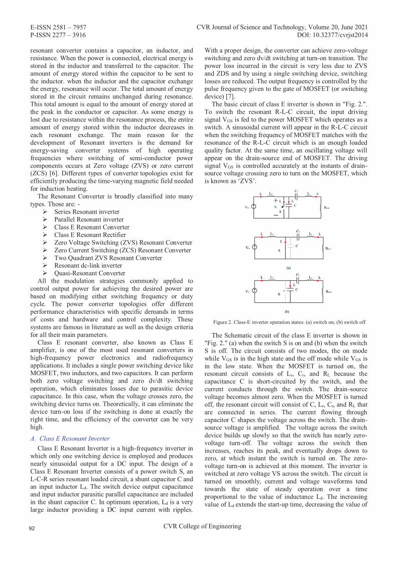
E-ISSN 2581 – 7957 P-ISSN 2277 – 3916
CVR Journal of Science and Technology, Volume 20, June 2021 DOI: 10.32377/cvrjst201
CVR College of Engineering
resonant converter contains a capacitor, an inductor, and resistance. When the power is connected, electrical energy is stored in the inductor and transferred to the capacitor. The amount of energy stored within the capacitor to be sent to the inductor. when the inductor and the capacitor exchange the energy, resonance will occur. The total amount of energy stored in the circuit remains unchanged during resonance. This total amount is equal to the amount of energy stored at the peak in the conductor or capacitor. As some energy is lost due to resistance within the resonance process, the entire amount of energy stored within the inductor decreases in each resonant exchange. The main reason for the development of Resonant inverters is the demand for energy-saving converter systems of high operating frequencies where switching of semi-conductor power components occurs at Zero voltage (ZVS) or zero current (ZCS) [6]. Different types of converter topologies exist for efficiently producing the time-varying magnetic field needed for induction heating.
The Resonant Converter is broadly classified into many types. Those are: -
� Series Resonant inverter � Parallel Resonant inverter � Class E Resonant Converter � Class E Resonant Rectifier � Zero Voltage Switching (ZVS) Resonant Converter � Zero Current Switching (ZCS) Resonant Converter � Two Quadrant ZVS Resonant Converter � Resonant dc-link inverter � Quasi-Resonant Converter
All the modulation strategies commonly applied to control output power for achieving the desired power are based on modifying either switching frequency or duty cycle. The power converter topologies offer different performance characteristics with specific demands in terms of costs and hardware and control complexity. These systems are famous in literature as well as the design criteria for all their main parameters.
Class E resonant converter, also known as Class E amplifier, is one of the most used resonant converters in high-frequency power electronics and radiofrequency applications. It includes a single power switching device like MOSFET, two inductors, and two capacitors. It can perform both zero voltage switching and zero dv/dt switching operation, which eliminates losses due to parasitic device capacitance. In this case, when the voltage crosses zero, the switching device turns on. Theoretically, it can eliminate the device turn-on loss if the switching is done at exactly the right time, and the efficiency of the converter can be very high.
A. Class E Resonant Inverter Class E Resonant Inverter is a high-frequency inverter in
which only one switching device is employed and produces nearly sinusoidal output for a DC input. The design of a Class E Resonant Inverter consists of a power switch S, an L-C-R series resonant loaded circuit, a shunt capacitor C and an input inductor Ld. The switch device output capacitance and input inductor parasitic parallel capacitance are included in the shunt capacitor C. In optimum operation, Ld is a very large inductor providing a DC input current with ripples.
With a proper design, the converter can achieve zero-voltage switching and zero dv/dt switching at turn-on transition. The power loss incurred in the circuit is very less due to ZVS and ZDS and by using a single switching device, switching losses are reduced. The output frequency is controlled by the pulse frequency given to the gate of MOSFET (or switching device) [7].
The basic circuit of class E inverter is shown in "Fig. 2.". To switch the resonant R-L-C circuit, the input driving signal VGS is fed to the power MOSFET which operates as a switch. A sinusoidal current will appear in the R-L-C circuit when the switching frequency of MOSFET matches with the resonance of the R-L-C circuit which is an enough loaded quality factor. At the same time, an oscillating voltage will appear on the drain-source end of MOSFET. The driving signal VGS is controlled accurately at the instants of drain-source voltage crossing zero to turn on the MOSFET, which is known as ‘ZVS’.
Figure 2. Class-E inverter operation states: (a) switch on; (b) switch off
The Schematic circuit of the class E inverter is shown in "Fig. 2." (a) when the switch S is on and (b) when the switch S is off. The circuit consists of two modes, the on mode while VGS is in the high state and the off mode while VGS is in the low state. When the MOSFET is turned on, the resonant circuit consists of Lr, Cr, and RL because the capacitance C is short-circuited by the switch, and the current conducts through the switch. The drain-source voltage becomes almost zero. When the MOSFET is turned off, the resonant circuit will consist of C, Lr, Cr, and RL that are connected in series. The current flowing through capacitor C shapes the voltage across the switch. The drain-source voltage is amplified. The voltage across the switch device builds up slowly so that the switch has nearly zero-voltage turn-off. The voltage across the switch then increases, reaches its peak, and eventually drops down to zero, at which instant the switch is turned on. The zero-voltage turn-on is achieved at this moment. The inverter is switched at zero voltage VS across the switch. The circuit is turned on smoothly, current and voltage waveforms tend towards the state of steady operation over a time proportional to the value of inductance Ld. The increasing value of Ld extends the start-up time, decreasing the value of
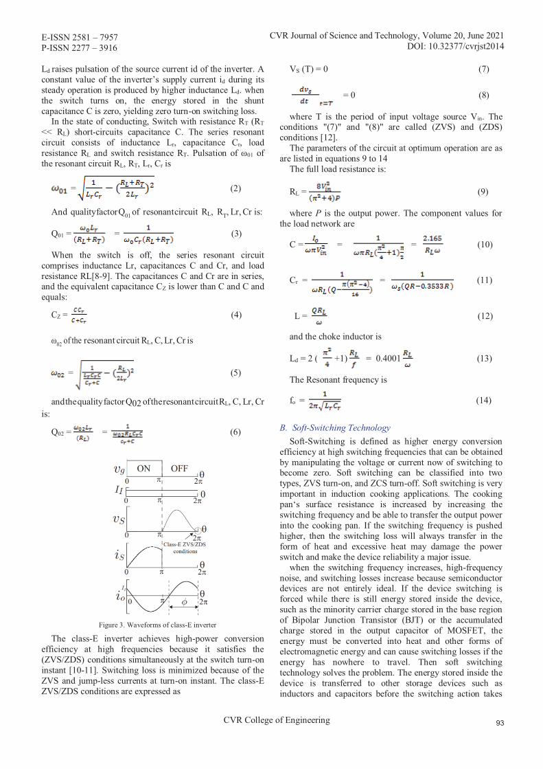
E-ISSN 2581 – 7957 P-ISSN 2277 – 3916
CVR College of Engineering
Ld raises pulsation of the source current id of the inverter. A constant value of the inverter’s supply current id during its steady operation is produced by higher inductance Ld. when the switch turns on, the energy stored in the shunt capacitance C is zero, yielding zero turn-on switching loss.
In the state of conducting, Switch with resistance RT (RT << RL) short-circuits capacitance C. The series resonant circuit consists of inductance Lr, capacitance Cr, load resistance RL and switch resistance RT. Pulsation of ω01 of the resonant circuit RL, RT, Lr, Cr is
= (2)
And quality factor Q01 of resonant circuit RL, RT, Lr, Cr is:
Q01 = = (3)
When the switch is off, the series resonant circuit comprises inductance Lr, capacitances C and Cr, and load resistance RL[8-9]. The capacitances C and Cr are in series, and the equivalent capacitance CZ is lower than C and C and equals:
CZ = (4)
ω02 of the resonant circuit RL, C, Lr, Cr is
= (5)
and the quality factor Q02 of the resonant circuit RL, C, Lr, Cr is:
Q02 = = (6)
Figure 3. Waveforms of class-E inverter
The class-E inverter achieves high-power conversion efficiency at high frequencies because it satisfies the (ZVS/ZDS) conditions simultaneously at the switch turn-on instant [10-11]. Switching loss is minimized because of the ZVS and jump-less currents at turn-on instant. The class-E ZVS/ZDS conditions are expressed as
VS (T) = 0 (7)
= 0 (8)
where T is the period of input voltage source Vin. The conditions "(7)" and "(8)" are called (ZVS) and (ZDS) conditions [12].
The parameters of the circuit at optimum operation are as are listed in equations 9 to 14
The full load resistance is:
RL = (9)
where P is the output power. The component values for the load network are
C = = = (10)
Cr = = (11)
L = (12)
and the choke inductor is
Ld = 2 (( +1) = 0.4001 (13)
The Resonant frequency is
fo = (14)
B. Soft-Switching Technology Soft-Switching is defined as higher energy conversion
efficiency at high switching frequencies that can be obtained by manipulating the voltage or current now of switching to become zero. Soft switching can be classified into two types, ZVS turn-on, and ZCS turn-off. Soft switching is very important in induction cooking applications. The cooking pan‘s surface resistance is increased by increasing the switching frequency and be able to transfer the output power into the cooking pan. If the switching frequency is pushed higher, then the switching loss will always transfer in the form of heat and excessive heat may damage the power switch and make the device reliability a major issue.
when the switching frequency increases, high-frequency noise, and switching losses increase because semiconductor devices are not entirely ideal. If the device switching is forced while there is still energy stored inside the device, such as the minority carrier charge stored in the base region of Bipolar Junction Transistor (BJT) or the accumulated charge stored in the output capacitor of MOSFET, the energy must be converted into heat and other forms of electromagnetic energy and can cause switching losses if the energy has nowhere to travel. Then soft switching technology solves the problem. The energy stored inside the device is transferred to other storage devices such as inductors and capacitors before the switching action takes
CVR Journal of Science and Technology, Volume 20, June 2021 DOI: 10.32377/cvrjst201
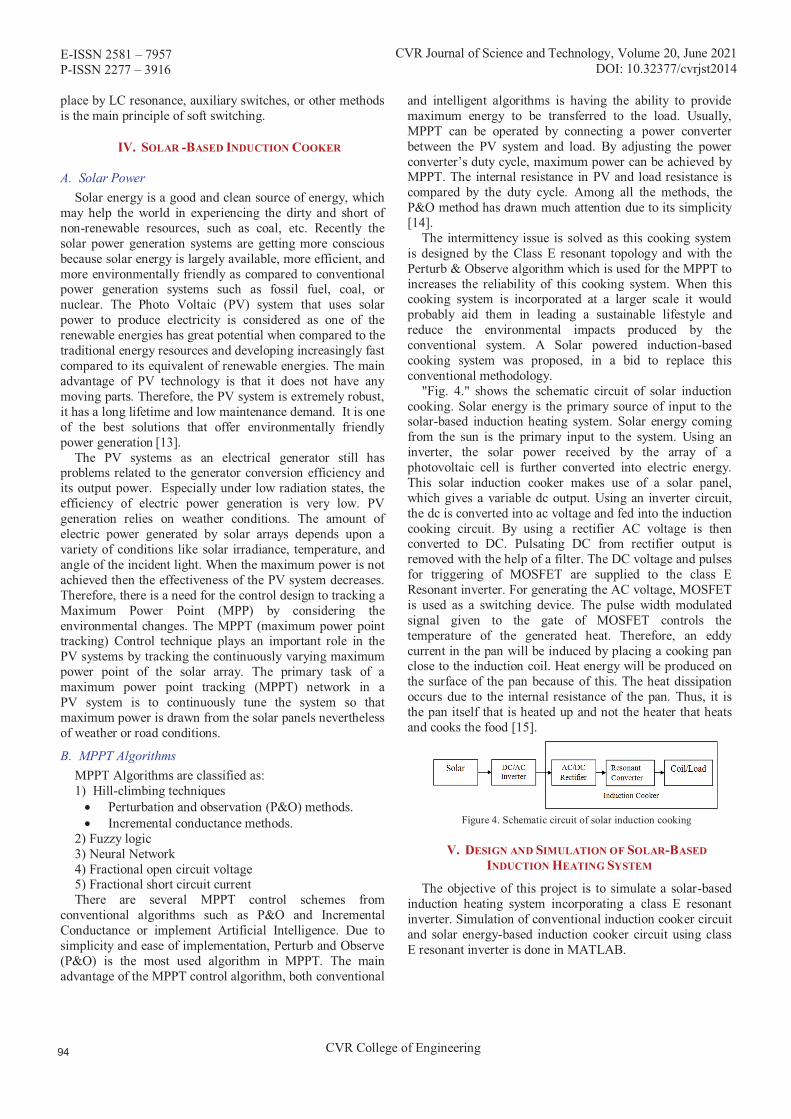
E-ISSN 2581 – 7957 P-ISSN 2277 – 3916
CVR College of Engineering
place by LC resonance, auxiliary switches, or other methods is the main principle of soft switching.
IV. SOLAR -BASED INDUCTION COOKER
A. Solar Power Solar energy is a good and clean source of energy, which
may help the world in experiencing the dirty and short of non-renewable resources, such as coal, etc. Recently the solar power generation systems are getting more conscious because solar energy is largely available, more efficient, and more environmentally friendly as compared to conventional power generation systems such as fossil fuel, coal, or nuclear. The Photo Voltaic (PV) system that uses solar power to produce electricity is considered as one of the renewable energies has great potential when compared to the traditional energy resources and developing increasingly fast compared to its equivalent of renewable energies. The main advantage of PV technology is that it does not have any moving parts. Therefore, the PV system is extremely robust, it has a long lifetime and low maintenance demand. It is one of the best solutions that offer environmentally friendly power generation [13].
The PV systems as an electrical generator still has problems related to the generator conversion efficiency and its output power. Especially under low radiation states, the efficiency of electric power generation is very low. PV generation relies on weather conditions. The amount of electric power generated by solar arrays depends upon a variety of conditions like solar irradiance, temperature, and angle of the incident light. When the maximum power is not achieved then the effectiveness of the PV system decreases. Therefore, there is a need for the control design to tracking a Maximum Power Point (MPP) by considering the environmental changes. The MPPT (maximum power point tracking) Control technique plays an important role in the PV systems by tracking the continuously varying maximum power point of the solar array. The primary task of a maximum power point tracking (MPPT) network in a PV system is to continuously tune the system so that maximum power is drawn from the solar panels nevertheless of weather or road conditions.
B. MPPT Algorithms MPPT Algorithms are classified as: 1) Hill-climbing techniques� Perturbation and observation (P&O) methods. � Incremental conductance methods.
2) Fuzzy logic3) Neural Network4) Fractional open circuit voltage5) Fractional short circuit currentThere are several MPPT control schemes from
conventional algorithms such as P&O and Incremental Conductance or implement Artificial Intelligence. Due to simplicity and ease of implementation, Perturb and Observe (P&O) is the most used algorithm in MPPT. The main advantage of the MPPT control algorithm, both conventional
and intelligent algorithms is having the ability to provide maximum energy to be transferred to the load. Usually, MPPT can be operated by connecting a power converter between the PV system and load. By adjusting the power converter’s duty cycle, maximum power can be achieved by MPPT. The internal resistance in PV and load resistance is compared by the duty cycle. Among all the methods, the P&O method has drawn much attention due to its simplicity
[14]. The intermittency issue is solved as this cooking system
is designed by the Class E resonant topology and with the Perturb & Observe algorithm which is used for the MPPT to increases the reliability of this cooking system. When this cooking system is incorporated at a larger scale it would probably aid them in leading a sustainable lifestyle and reduce the environmental impacts produced by the conventional system. A Solar powered induction-based cooking system was proposed, in a bid to replace this conventional methodology.
"Fig. 4." shows the schematic circuit of solar induction cooking. Solar energy is the primary source of input to the solar-based induction heating system. Solar energy coming from the sun is the primary input to the system. Using an inverter, the solar power received by the array of a photovoltaic cell is further converted into electric energy. This solar induction cooker makes use of a solar panel, which gives a variable dc output. Using an inverter circuit, the dc is converted into ac voltage and fed into the induction cooking circuit. By using a rectifier AC voltage is then converted to DC. Pulsating DC from rectifier output is removed with the help of a filter. The DC voltage and pulses for triggering of MOSFET are supplied to the class E Resonant inverter. For generating the AC voltage, MOSFET is used as a switching device. The pulse width modulated signal given to the gate of MOSFET controls the temperature of the generated heat. Therefore, an eddy current in the pan will be induced by placing a cooking pan close to the induction coil. Heat energy will be produced on the surface of the pan because of this. The heat dissipation occurs due to the internal resistance of the pan. Thus, it is the pan itself that is heated up and not the heater that heats and cooks the food [15].
Figure 4. Schematic circuit of solar induction cooking
V. DESIGN AND SIMULATION OF SOLAR-BASEDINDUCTION HEATING SYSTEM
The objective of this project is to simulate a solar-based induction heating system incorporating a class E resonant inverter. Simulation of conventional induction cooker circuit and solar energy-based induction cooker circuit using class E resonant inverter is done in MATLAB.
CVR Journal of Science and Technology, Volume 20, June 2021 DOI: 10.32377/cvrjst201

E-ISSN 2581 – 7957 P-ISSN 2277 – 3916
CVR College of Engineering
Figure 5. Conventional adaptor-based induction heating system with resonant E converter
Induction heating is a popular technique for producing very high heat in a fraction of time. Induction cooking is one of the applications of induction heating that is employed for residential and commercial usage. High power factor and low line current are achieved with the help of class E resonant inverter, which is very interesting in terms of commercial production. With a very high rate of change within the magnetic field, a high-frequency AC flowing through the coil provides the proper heat which is useful for cooking.
To increase the frequency and for the wiring protection, induction cook tops consist of electronic devices. The frequency at the coil is very large than the input frequency (generally, more than 1000 times). Induction cookware is generally made up of ferrous metals because these are relatively poor conductors of electricity, so they have high resistance. When a current is passed through a high resistive material, much of the current is converted into heat energy. The heat energy which is used to cook food on an induction cook top comes from this electrical resistance and changes in the magnetic field of the cookware.
A. Simulation of Conventional Induction Heating System ‘ Fig. 5,’ shows the main Circuit with a conventional
adaptor-based induction heating system with Class E Resonant Converter. The circuit consists of 4 parts: rectifier, filter, high-frequency inverter, and resonant load. The rectifier module is a full-bridge rectifier (D1, D2, D3, D4). The second portion of the system is a capacitive filter (Lf, Cf). The ripple components are minimized by this filter. The third is a high-frequency converter (Class E Resonant Inverter) to convert the constant DC to high-frequency AC by switching the MOSFET which is used as a power source and can be driven by the pulse signals. PWM generator is used for pulse generation. High-frequency alternating current is generated in the Resonant Load (Lr, Cr, RL). The parameters used for the filtering side and the resonant converter are given in below table II.
TABLE II. PARAMETERS
Parameter Expanded
Symbol Value of the parameter
Input Voltage V 220 V
Filter Inductor Lf 500 μH
Filter Capacitance
Cf 4.7 μF
Choke Inductor Ld 31.83 μH
Shunt Capacitor
C 1.7229 μF
Resonant Inductor
Lr 517.042 μH
Resonant Capacitance
Cr 0.10μF
Resistance Req 10Ω
AC supply of 220V is applied as input to the circuit. During the positive half cycle, the diodes D1, D4 operate. Mode 1 is active when the switch is ON. PWM pulses generation for the class E converter with a duty cycle of 50% is shown in "Fig. 6". During mode 1, the active switch is turned ON with ZVS, the current flows through Ld. The resonant circuit consists of Lr, Cr, and RL because the capacitance C is short-circuited by the switch, and the current conducts through the switch. The drain-source voltage becomes almost zero. The current through the switch increases till the switch gets off. During the negative half-cycle, the diodes D2 and D3 of the bridge rectifier will operate. Mode 2 is activated when Q is turned OFF. The resonant circuit will consist of C, Lr, Cr, and RL that are connected in series. The current flowing through capacitor C shapes the voltage across the switch. The drain-source voltage is amplified. The voltage across the switch device builds up slowly so that the switch has nearly zero-voltage turn-off. The voltage across the switch then increases, reaches its peak, and eventually drops down to zero, at which instant the switch is turned on.
CVR Journal of Science and Technology, Volume 20, June 2021 DOI: 10.32377/cvrjst201
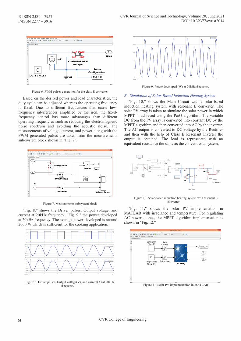
E-ISSN 2581 – 7957 P-ISSN 2277 – 3916
CVR College of Engineering
Figure 6. PWM pulses generation for the class E converter
Based on the desired power and load characteristics, the duty cycle can be adjusted whereas the operating frequency is fixed. Due to different frequencies that cause low-frequency interferences amplified by the iron, the fixed-frequency control has more advantages than different operating frequencies such as reducing the electromagnetic noise spectrum and avoiding the acoustic noise. The measurements of voltage, current, and power along with the PWM generated pulses are taken from the measurements sub-system block shown in "Fig. 7".
Figure 7. Measurements subsystem block
"Fig. 8,” shows the Driver pulses, Output voltage, and current at 20kHz frequency. "Fig. 9," the power developed at 20kHz frequency. The average power developed is around 2000 W which is sufficient for the cooking application.
Figure 8. Driver pulses, Output voltage(V), and current(A) at 20kHz frequency
Figure 9. Power developed (W) at 20kHz frequency
B. Simulation of Solar-Based Induction Heating System "Fig. 10,” shows the Main Circuit with a solar-based
induction heating system with resonant E converter. The solar PV array is taken to simulate the solar power in which MPPT is achieved using the P&O algorithm. The variable DC from the PV array is converted into constant DC by the MPPT algorithm and then converted into AC by the inverter. The AC output is converted to DC voltage by the Rectifier and then with the help of Class E Resonant Inverter the output is obtained. The load is represented with an equivalent resistance the same as the conventional system.
Figure 10. Solar-based induction heating system with resonant E converter
"Fig. 11," shows the solar PV implementation in MATLAB with irradiance and temperature. For regulating AC power output, the MPPT algorithm implementation is shown in "Fig. 12."
Figure 11. Solar PV implementation in MATLAB
CVR Journal of Science and Technology, Volume 20, June 2021 DOI: 10.32377/cvrjst201
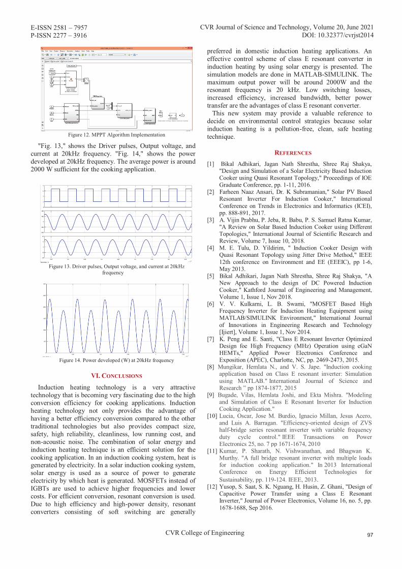
E-ISSN 2581 – 7957 P-ISSN 2277 – 3916
CVR College of Engineering
Figure 12. MPPT Algorithm Implementation
"Fig. 13," shows the Driver pulses, Output voltage, and current at 20kHz frequency. "Fig. 14," shows the power developed at 20kHz frequency. The average power is around 2000 W sufficient for the cooking application.
Figure 13. Driver pulses, Output voltage, and current at 20kHz frequency
Figure 14. Power developed (W) at 20kHz frequency
VI. CONCLUSIONS
Induction heating technology is a very attractive technology that is becoming very fascinating due to the high conversion efficiency for cooking applications. Induction heating technology not only provides the advantage of having a better efficiency conversion compared to the other traditional technologies but also provides compact size, safety, high reliability, cleanliness, low running cost, and non-acoustic noise. The combination of solar energy and induction heating technique is an efficient solution for the cooking application. In an induction cooking system, heat is generated by electricity. In a solar induction cooking system, solar energy is used as a source of power to generate electricity by which heat is generated. MOSFETs instead of IGBTs are used to achieve higher frequencies and lower costs. For efficient conversion, resonant conversion is used. Due to high efficiency and high-power density, resonant converters consisting of soft switching are generally
preferred in domestic induction heating applications. An effective control scheme of class E resonant converter in induction heating by using solar energy is presented. The simulation models are done in MATLAB-SIMULINK. The maximum output power will be around 2000W and the resonant frequency is 20 kHz. Low switching losses, increased efficiency, increased bandwidth, better power transfer are the advantages of class E resonant converter. This new system may provide a valuable reference to decide on environmental control strategies because solar induction heating is a pollution-free, clean, safe heating technique.
REFERENCES [1] Bikal Adhikari, Jagan Nath Shrestha, Shree Raj Shakya,
"Design and Simulation of a Solar Electricity Based Induction Cooker using Quasi Resonant Topology," Proceedings of IOE Graduate Conference, pp. 1-11, 2016.
[2] Farheen Naaz Ansari, Dr. K Subramanian," Solar PV Based Resonant Inverter For Induction Cooker," International Conference on Trends in Electronics and Informatics (ICEI), pp. 888-891, 2017.
[3] A. Vijin Prabhu, P. Jeba, R. Babu, P. S. Samuel Ratna Kumar, "A Review on Solar Based Induction Cooker using Different Topologies," International Journal of Scientific Research and Review, Volume 7, Issue 10, 2018.
[4] M. E. Tulu, D. Yildirim, " Induction Cooker Design with Quasi Resonant Topology using Jitter Drive Method," IEEE 12th conference on Environment and EE (EEEIC), pp 1-6, May 2013.
[5] Bikal Adhikari, Jagan Nath Shrestha, Shree Raj Shakya, "A New Approach to the design of DC Powered Induction Cooker," Kathford Journal of Engineering and Management, Volume 1, Issue 1, Nov 2018.
[6] V. V. Kulkarni, L. B. Swami, "MOSFET Based High Frequency Inverter for Induction Heating Equipment using MATLAB/SIMULINK Environment," International Journal of Innovations in Engineering Research and Technology [Ijiert], Volume 1, Issue 1, Nov 2014.
[7] K. Peng and E. Santi, "Class E Resonant Inverter Optimized Design foe High Frequency (MHz) Operation using eGaN HEMTs," Applied Power Electronics Conference and Exposition (APEC), Charlotte, NC, pp. 2469-2473, 2015.
[8] Mungikar, Hemlata N., and V. S. Jape. "Induction cooking application based on Class E resonant inverter: Simulation using MATLAB." International Journal of Science and Research ” pp 1874-1877, 2015
[9] Bugade, Vilas, Hemlata Joshi, and Ekta Mishra. "Modeling and Simulation of Class E Resonant Inverter for Induction Cooking Application."
[10] Lucia, Oscar, Jose M. Burdio, Ignacio Millan, Jesus Acero, and Luis A. Barragan. "Efficiency-oriented design of ZVS half-bridge series resonant inverter with variable frequency duty cycle control." IEEE Transactions on Power Electronics 25, no. 7 pp 1671-1674, 2010
[11] Kumar, P. Sharath, N. Vishwanathan, and Bhagwan K. Murthy. "A full bridge resonant inverter with multiple loads for induction cooking application." In 2013 International Conference on Energy Efficient Technologies for Sustainability, pp. 119-124. IEEE, 2013.
[12] Yusop, S. Saat, S. K. Nguang, H. Husin, Z. Ghani, "Design of Capacitive Power Transfer using a Class E Resonant Inverter," Journal of Power Electronics, Volume 16, no. 5, pp. 1678-1688, Sep 2016.
CVR Journal of Science and Technology, Volume 20, June 2021 DOI: 10.32377/cvrjst201

E-ISSN 2581 – 7957 P-ISSN 2277 – 3916
CVR College of Engineering
[13] Bandile I. Sibiya, Dr. Chitra Venugopal, "Solar Powered Induction Cooking System," 1st International Conference on Power Engineering, Computing and Control, PECCON-2017, 24 March 2017.
[14] A. C. Subrata, T. Sutikno, S. Padmanaban, and H. S. Purnama, "Maximum Power Point Tracking in PV Arrays with High Gain DC-DC Boost Converter," 6th International
Conference on Electrical Engineering, Computer Science and Informatics (EECSI), pp. 358-362, 2019.
[15] Vilas Bugade, Hemlata Joshi, Ekta Mishra, "Modeling and Simulation of Class E Resonant Inverter for Induction Cooking Application," International Journal of Engineering Trends and Technology (IJETT), Volume 60, Issue 1, June 2018.
CVR Journal of Science and Technology, Volume 20, June 2021 DOI: 10.32377/cvrjst201
E-ISSN 2581 – 7957 CVR Journal of Science and Technology, Volume 20, June 2021 P-ISSN 2277 – 3916 DOI: 10.32377/cvrjst2015
CVR College of Engineering
Cleaning of Solar Panel using Automation Technique
Sairaj1 and Dr. K. Shashidhar Reddy2
Email: [email protected] 2Professor, CVR College of Engineering India
Email: [email protected]
Abstract: Solar energy is considered to be one of the best major renewable energy resources to generate and meet the electrical energy demand of the entire globe. Solar PV modules produce electricity by collecting the sunlight. solar PV modules
India, which comes under the tropical region. Various dust particles present in the tropical region, so the dust particles are accumulated on the surface of the solar panel. Therefore, the incident light can be blocked. As a result, the module power capacity can be reduced. If the panel not cleaned properly the power output become reduced by 50%. To increase the power output an automatic cleaning mechanism has been designed. This automatic cleaning mechanism not only senses the dust accumulated on the solar panel but also clean the solar PV module automatically. This solar cleaning mechanism is mainly implemented using PIC 16F 1527 microcontroller, which mainly controls the stepper motor, Air compressor and water pump. The dust can be cleaned by the gantry which is mainly driven by the stepper motor. The gantry has mist nozzles which create pressurized air and water to clean the solar panel effectively. The cleaning can be done by air and water depending upon the dust accumulated on the solar panel.
Index Terms: solar panel; micro-controller; stepper motor; dust particles.
I. INTRODUCTION
The Solar panel cleaning mechanism is one of the best methods to clean the accumulated dust on the solar panel. Renewable energy resources have a major contribution to distributed generation. Solar energy plays a vital role in producing the distributed generation. Solar panels are used as the main power source for most the applications like agriculture, industrial as well as domestic applications. There are many types of solar panels. Dust build-up on solar module surface is an issue of great worry, particularly in desert provinces regular dust storms occur. The glass cover transmittance decreases because of the accretion of dust on the surface of the PV module, which ultimately decreases the amount of solar irradiation reaching the cells [1]. The dust density of the surface, orientation, the tilt angle, exposure period, dominant wind direction, and site climatic conditions are the main key factors to reduce the glass transmittance. The dusty environment countries produce a lot of dust on the solar panel as a result the transmittance of solar energy reduces on the solar panel. India faces this kind of problem. The accumulated dust decreases the tilt angle as a result sufficient amount of solar energy is not produced; the best way to eliminate the accumulated dust on the environment is to clean the solar panel.
In some places, the cleaning process is very complex for humans. This complexity can be reduced after the invention of an automation cleaning mechanism like an autonomous robot (Gantry). Gantry cleaning is the most effective way of cleaning in recent years. Gantry cleaner is an autonomous device that can move around and clean the surface using different techniques such as air and water jet cleaning. The proposed solar panel cleaning system falls in the category of cleaning gantry mechanism, but for industrial cleaning application in large scale solar power plants [2]. Dust may be defined as crushed form which is in the form of hundreds of microns. Dust may come in the environment from various sources such as construction sites, industries and other dust produced areas. Dust consists of floating invisible, visible and fallen particles of solid material. The authors have compared the various dust particles present on the solar panels, which mainly degrade the efficiency of solar panel. They also reported that a small amount of dust on the solar PV module creates a blockage for solar incident rays. Researchers conducted studies on the effect of different influential parameters on the efficiency and performance of PV cells [3]. Solar panels can be cleaned by two ways, they are: 1. Manual cleaning2. Automatic cleaning using gantry
1. Manual Cleaning:This type of cleaning is tedious, cumbersome and also
expensive in terms of the labor involved and time. It requires more manual setup and time consumption. To clean the solar panel manually has the following disadvantages [3].
1.1 Non-Uniform Pressure During The Cleaning: Manually, the pressure exerting on the solar panel is not
always equal. With too high pressure the panels can be damaged in the worst case. If the pressure on the other hand is too low, the surface will not be thoroughly cleaned.
1.2 It Is Not Possible To Manually Clean The Whole Solar Panel Surface:
Solar panels constructed at a certain height have corners and sides that are difficult to reach. It is very difficult even if we use scrubber.
1.3 People Become Tired And Made Mistakes: The solar PV panels occupy more surface areas so
cleaning the total solar panels with manual set up require more time [3]. The following are the common human errors:
� Panel surface areas are not cleaned properly.
are generally employed in dusty environmental areas like in
1 PG Scholar, CVR College of Engineering/ E E Department, Hyderabad, India

E-ISSN 2581 – 7957 CVR Journal of Science and Technology, Volume 20, June 2021 P-ISSN 2277 – 3916 DOI: 10.32377/cvrjst2015
CVR College of Engineering
� A wrong or sudden movement can cause scratches.
1.4 Manual Cleaning Solar Panels Are Not Always Safe: There are two important aspects to clean the solar
panels.
� Safety of PV Installation: As mentioned above, manual cleaning entails a potential
risk. Your valuable installation can be accidently damaged by human error [4].
� Safety of Cleaning Team: Cleaning staff often work in dangerous circumstances
during cleaning of the solar panel. There is particularly a risk of accidents when the panels are installed at a certain height [2].
Because of above disadvantages the manual cleaning of solar panel is time consuming and laborious. In order to overcome the above disadvantages, we prefer the automation cleaning [5].
Figure1. Manual cleaning.
2. Automatic Cleaning Using Gantry: This is the most innovative way of cleaning solar panels with the help of a microcontroller. This type of cleaning is very advantageous over manual cleaning since it doesn't require labour. It consumes very little time to clean the solar panels [6]. The following are the desired functions of an automated solar panel cleaning system: To cover cleaning area of solar panel in minimum amount of time. � To cover the cleaning area of solar panel in a minimum
amount of time. � To use a high-velocity water jet for cleaning. � To automate the water jet gantry movement in forward
and reverse directions. � To control the speed of movement of the gantry. � To automatically detect the edges of the panels and stop
the gantry movement. � To automatically switch on or switch off the gantry, air
compressor and water pump. � To control the cleaning cycle as per the given schedule. � To estimate the dust using water and air-jet cleaning
equipment. � To estimate the overall cost for cleaning the 1MW
capacity of panels based on this component.
� To implement control algorithm on an embedded controller.
� To identify and select the high-velocity jet nozzles. � To size the water pump suitable for the nozzles. � To understand air jet cleaning in place of water jet
cleaning. � To identify air jet nozzles suitable for dusting. � We can easily analyze the mechanical design of the
supporting structure. � We can easily clean the edges and corners of the entire
solar panel. Automatic cleaning is an accurate cleaning and improves the efficiency of the solar panel and reduces the consumption of water [7].
Figure 2. Automation cleaning.
II. PROPOSED METHOD
Initially provide power supply to the control panel which has the control components of the entire cleaning mechanism. In the control panel, we have a control circuit, protection relays, contactors and optocoupler. After Switch on the control panel, the converted power through SMPS enter into the CPU board. The CPU board consists of control and conversion components. The control panel can be operated either manually or automatically.
2.1. Manual Mode: � First switch on the air compressor and fill the
compressor with air up to its maximum level. � Now press the push buttons to run the gantry in a
forward direction. � The gantry can be driven with the help of a stepper
motor, i.e., the gantry moves in both forward and backward direction by a stepper motor.
� Now activate solenoid valve 1, so the compressed air comes through the nozzles and cleans the accumulated dust on the solar panel. The Air jet cleaning process is during the forward direction of the gantry.
� When the gantry reached to the desired length, the gantry can be stopped with the help of home switch.

E-ISSN 2581 – 7957 CVR Journal of Science and Technology, Volume 20, June 2021 P-ISSN 2277 – 3916 DOI: 10.32377/cvrjst2015
CVR College of Engineering
� Now press the push button to run the gantry in a backward direction, after that press the water pump push button.
� Now activate solenoid valve2. The water comes through the gantry and cleans the panel in the backward direction.
� After reaching the gantry at the starting point, now stop the operation by using a push-button.
Figure3. solar panel cleaning system in manual mode.
2.2. Automatic Mode: � The total operation can be controlled by a
microcontroller (PIC 16F 1527). Now embedded the time to fill the air compressor and dump this value into the microcontroller.
� Now embedded the stepper motor control and gantry movement i.e., both forward and reverse direction phenomenon code can be dump into the microcontroller.
� Now embedded the solenoid valves operation code and the water pump switch on timing can be dump into the microcontroller.
� Embedded the time taken to reach the gantry at the desired length and maintain the delay operation can be dump into the microcontroller.
� Fix the time delay of 2 -3 seconds for each operation and dump this time delay microcontroller.
Both these modules can be operated manually as well as Automatic mode depending upon the type of conditions present at the plant location. The only difference in manual mode is, it requires manual support but Automatic mode does not require any manual support it Automatically cleans the solar panel, depending upon its time grading. The time interval fixed in a microcontroller, i.e., the time interval of gantry movement can be fixed in a microcontroller depending upon the weather condition.
Figure4. solar panel cleaning system in Auto mode.
III. BLOCK DIAGRAM
Figure3. Describes the block diagram of Aautomatic solar panel cleaner. It has various stages of operation.
Figure 5. Block diagram of Automatic solar panel cleaner.
IV. FLOW CHART
Figure 6. Flow chart of automatic solar panel cleaner.
stop

E-ISSN 2581 – 7957 CVR Journal of Science and Technology, Volume 20, June 2021 P-ISSN 2277 – 3916 DOI: 10.32377/cvrjst2015
CVR College of Engineering
V. CONTROL PANEL
Control panel mainly has the following components. 5.1. Main circuit 5.2. Stepper motor driver 5.3. Optocouplers 5.4. Relays and contactors
Figure 7. Control panel
5.1 Main Circuit (Central Processing Unit): Main circuit has the following components. 5.1.1. Micro controller (PIC 16 F 1527) 5.1.2. Switched mode power supply (SMPS) 5.1.3. Switching regulator 5.1.4. Capacitors, resistors 5.1.5. Male and female sockets
5.1.1. Microcontroller (PIC 16F 1527): It is the main component of main circuit, all the user
defined operations are programmed and they were embedded in this microcontroller. In automation of solar panel cleaner PIC 16F 1527 micro controller is used.
Figure 8. Micro controller PIC 16F 1527.
The PIC 16F 1527 micro controller has the following features:
� Only 49 Instructions
� Up to 28 Kbytes Linear Program Memory Addressing.
� Up to 1536 Bytes Linear Data Memory Addressing. � It has I/O Ports, Primary and data memory, and
EEPROM, UART, PWM Operation and I2C operation.
� Operating Speed: � DC – 20 MHz clock input at 2.5V � DC – 16 MHz clock input at 1.8V � DC – 200 ns instruction cycle The PIC 16F 1527 micro controller consist of the
following inherent features: � It has input and output ports � Primary and data memory � EEPROM � UART � PWM OPERATION � I2C operation
5.1.2. Switched Mode Power Supply (SMPS): Initially we provide supply to the control panel; control panel gets on with the help of SMPS. Which converts the voltage from 230V (AC) to 24V (DC). In this control panel we used (Mean well LRS-50-24) SMPS. It has the following features: � No load power consumption. � High operating temperature up to 700C. � LED indicator for power on
Figure.9. SMPS
5.1.3. Switching Regulator: Switching regulator is used to convert the voltage from
any dc voltage to desired optimal voltage, which is in the order of 5V, 10V etc. In control panel I have used LM 2576T switching regulator.

E-ISSN 2581 – 7957 CVR Journal of Science and Technology, Volume 20, June 2021 P-ISSN 2277 – 3916 DOI: 10.32377/cvrjst2015
CVR College of Engineering
Figure 10. Switching regulator.
5.1.4. Capacitors & Resistors: These are mainly used in control panel to control higher voltage and currents. Especially capacitors mainly used as a filters, which removes the unwanted ripples in a dc output.
Figure 11. Capacitors
5.1.5. Male & Female Sockets: Male and female sockets act as interface between one
terminal and other terminal in control panel.
Figure 12. Male and female sockets.
5.2. Stepper Motor Driver: Stepper motor is an electromechanical device which converts electrical pulses into discrete mechanical movements. Depending upon the step angle through which motor shaft rotates for each command pulse of input.
. Figure 13. Stepper motor driver.
Figure 14. Stepper motor (NEMA 23).
5.3. Optocoupler: Optocoupler is mainly used to isolate electrical connections in the form of light energy. In control panel we used the PC817 optocoupler. A basic optocoupler is shown below.

E-ISSN 2581 – 7957 CVR Journal of Science and Technology, Volume 20, June 2021 P-ISSN 2277 – 3916 DOI: 10.32377/cvrjst2015
CVR College of Engineering
Figure 15. Optocoupler PC 817 connections.
Figure 16. Optocoupler PC 187.
5.4. Relays & Contactors: This section describes the relays, contactors, which
mainly operate the air compressor and water pump.
5.4.1. SPDT Relays: The electromagnetic SPDT relays (JQ 3F-C-S-10-DC
24V) are used in automatic solar panel cleaner. The rating of this relay is � Coil voltage: 24V DC � Current: 10A, Coil power: 0.45W
Figure 17. SPDT Relay.
5.4.2 Contactors: The power-controlled contactors (LC 1E 12) are used in
automatic solar panel cleaner. The rating of contactors are as follows: Minimum Switching Current: � 5 mA for signalling circuit. � Minimum Switching Voltage: 17 V for signalling
circuit � Non-Overlap Time: 1.5 ms on energisation between NC
and NO contact, 1.5 ms on de-energisation between NC and NO contact
� Insulation Resistance: > 10 MΩ for signalling circuit.
Figure 18. Contactors.
Relay and contactors are mainly used to operate the Air compressor and water pump. Whenever abnormal conditions will occur in the circuit then the contactor isolates the air compressor and water pump connections.
5.4.3 Water Pump: This water pump is mainly used to clean the solar panel
to create optimum amount of pressure to remove dust on solar panel through water.
� Horse Power: 1H.P � Max Current: 5A � Rotational Speed: 2800rpm � Head: 25m
Figure 19. Water pump.

E-ISSN 2581 – 7957 CVR Journal of Science and Technology, Volume 20, June 2021 P-ISSN 2277 – 3916 DOI: 10.32377/cvrjst2015
CVR College of Engineering
5.4.4 Air Compressor: Air compressor is mainly used to clean the solar panel to create optimum amount of pressure to remove dust on solar panel through air. � Max. pressure: 8 bar � Tank volume: 24 Liter � Air displacement:161 liter/min � Horse power: 1.5 hp � Powerful pump, less than 2 minutes to fill the tank to
maximum pressure.
Figure 20. Air compressor
Not only these components used in solar panel cleaner, but also used the following components they are:
v. Solenoid valve vi. Nozzles vii. Aluminium pipe viii. Screw rod ix. Aluminium extrusion x. Guide bars
5.4.5 Solenoid Valve: Solenoid valves are control units, which are electrically
energized or de energized. Whenever we provide electrical supply to the solenoid, the valve will automatically open and provides path for water as well as air flow.
In solar panel cleaner two solenoid valves are present, one is for air and one is for water.
Figure 21. Solenoid valve
5.4.6 Nozzles: In solar panel cleaner the Nozzles play vital role to
conserve water,and the air flow can be very high.i.e. It creates high pressure,which is main advantageous to clean the solar panel.
Figure 22.Mist Nozzles
5.4.7 Aluminium Pipe: � An 25.4mm OD Aluminum pipe with 3mm
thickness has been used to attach nozzles. � The pipe has been drilled at regular intervals along
the length.
Figure 23.Aluminium pipe.
5.4.8 Screw Rod: M12 ISO Metric threaded screw rod suspended at both
ends on ball bearings and coupled to stepper motor has been used to move gantry along the solar panels
� Pitch: 1.6mm � Diameter: 12mm � Length: 2000mm

E-ISSN 2581 – 7957 CVR Journal of Science and Technology, Volume 20, June 2021 P-ISSN 2277 – 3916 DOI: 10.32377/cvrjst2015
CVR College of Engineering
Figure 24.Screw rod.
5.4.9 Aluminium Extrusion: Aluminium extrusion is mainly used to guide the wheels to move forward as well as reverse direction.It provides free movement to the guide bars.
Figure 25. Aluminium extrusion.
5.4.10 Guide bars: 20X40 Aluminum extrusion along with delrin wheels has
been used as guide bars for the gantry.
Figure 26. Guide bars.
VI. FINAL RESULTS
With the help of solar panel, the following results are observed: � The optimum amount of water can be utilised by this
solar panel cleaner. Manually it takes 25 litres of water to clean two solar panels. With the help of solar panel cleaner, it takes around 0.5-1 litres of water.
� The solar panel can be cleaned at any time as per our requirement. Generally, regular interval of time is preferable, depending upon the dust accumulation on the solar panel.
� The efficiency of solar panel increased effectively. TABLE I.
P-V VALUES WHEN DUST ACCUMULATION ON SOLAR PANEL.
DATE DAY VOLTAGE (V) POWER (W)
01-02-2020 I 32 125
02-02-2020 II 29 119
03-02-2020 III 24 104
04-02-2020 IV 21 99
05-02-2020 V 20 85
06-02-2020 VI 22 70
07-02-2020 VII 21 60
AVERAGE POWER(W) 94.57
TABLE II. P-V VALUES AFTER CLEANING THE SOLAR PANEL.
DATE DAY VOLTAGE (V) POWER (W)
01-02-2020 I 40 155
02-02-2020 II 39 152
03-02-2020 III 36 150
04-02-2020 IV 35 149
05-02-2020 V 37 150
06-02-2020 VI 38 151
07-02-2020 VII 39 150
AVERAGE POWER(W) 151
By considering the above results the following observations were obtained: The power and voltage values gradually decrease because of the dust accumulated on the solar panel, where the values are considered for one solar panel under offload condition. � From table I. (PV values when dust accumulated on the
solar panel), depicts that the voltage and power levels are reduced. As a result, the efficiency of the solar panel reduces.
� From table II. (PV values when the dust cleared by solar panel cleaner), observed that the power and voltage values are slightly reduced when compared to table I. Reduction is due to the uneven dust deposition from the day I - day VII, i.e., the dust cannot be predicted exactly the day by day. The efficiency of the solar panel increased when the dust was cleared on the solar panel.
E-ISSN 2581 – 7957 CVR Journal of Science and Technology, Volume 20, June 2021 P-ISSN 2277 – 3916 DOI: 10.32377/cvrjst2015
CVR College of Engineering
The performance of solar panel can be improved effectively by using the solar panel cleaning. The efficiency can be calculated as follows:
The efficiency of solar panel can be degraded as follows: � The weather condition plays very important role in
the solar panel efficiency such as sun intensity, humidity, and huge amount of heat dissipation.
� Dust particles and bird drops also one of the major reasons to degrade the efficiency.
� Low quality material is used in the solar P-V cells also caused to reduce the efficiency of solar panel.
Efficiency comparison between the solar panels using automation and without using automation is as follows:
� Efficiency of solar panel without using Automation:
Ƞ = 94.57 *100
500 Ƞ = 18.91 %
Note: Average power considered from TABLE I. � Efficiency of solar panel using Automation:
Ƞ = 151 *100
500
Ƞ = 30.20 %
Note: Average power considered from TABLE II. Initially, the power and voltage can be in optimum value in both cases, i.e., the solar panel is using with automation and without automation.Whenever the dust accumulated on the surface of the solar panel, the output power and voltage can be dropped gradually. From table I, we conclude that the voltage and power levels are dropped gradually from the day I - day VII. As a result, the efficiency was not better, which is disadvantageous to the consumers. From table II, we conclude that the voltage and power levels from day I - day VII are much better than table I, i.e., the efficiency of a solar panel with automation is better than the efficiency of a solar panel without using automation.
3.1. Characteristics:
0
20
40
60
80
100
120
140
I I III V VII
V0LTAGE (V)
POWER (W)
DAY
Figure27. P-V characteristics of solar panel without solar panel cleaner.
020406080
100120140160180
I I III V VII
V0LTAGE (V)
POWER (W)
DAY
Figure28.P-V characteristics of solar panel using solar panel
Cleaner.
020406080
100120140160180
I I III V VII
POWER (W)WITHCLEANER
POWER (W)WITHOUTCLEANER
DAY
Figure 29. Comparing the power of solar panel, with and without using solar panel cleaner.

E-ISSN 2581 – 7957 CVR Journal of Science and Technology, Volume 20, June 2021 P-ISSN 2277 – 3916 DOI: 10.32377/cvrjst2015
CVR College of Engineering
VII. CONCLUSIONS
In a solar panel, cleaner designing is a very important task, thereafter controlling mechanism. During the cleaning mechanism some observations were made: � The linear actuator system working was very nice, so it
achieves the desired system parameter. � Using screw rod some unstable disturbances occur,
therefore some changes are necessary for the screw mechanism.
� There is a chance of reducing the weight of the gantry. As a result, the thrust can be reduced on the panel.
� The scrubber should attach with the gantry; therefore, the cleaning process is much efficient, i.e., the sticky dust can be removed on the solar panel.
VIII. FUTURE SCOPE
Automatic solar panel cleaner requires the following modifications, which can be improved as follows: � To clean 1 MW plant area of solar panels, in a short
interval of time. � To maintain the cleaning mechanism should be
uniform. � An automatic weather detector mechanism should be
included in this solar panel cleaner. � Weather forecasting data should include in this
mechanism. � A dust analyser should include in this mechanism.
REFERENCES [1] R.E.P.N. for the 21st Century, “Renewable 2012, global status
report”., tech.rep., [2] J. Zorilla-Casanova, “Analysis of dust losses in Photovoltaic
modules” of world renewable Energy Congress2011.Sweden, 8-13 May 2011.
[3] Katz.G. (2008, 27 April 2011),” Effect of dust on Solar panel”. Available: www.gregorybkatz.com.
[4] Shaharin A. Suleiman, Haizatul,” Energy efficiency of solar panel”. Indian streams research journal ISSN 2230-7850.
[5] K.A. Moharram, M.S. Abd - Elhady, H.A. K and H. El-Sheriff,” Influence of cleaning using water and surfactants on performance of photovoltaic panels”. Energy convers. Manage., vol.68, pp.266272,2013. DOI: 10.1016/j.enconman.2013.01.022.
[6] Mohammad A. Bou-Rabee,” Influence of Dirt Accumulation on performance of PV panels. “Available: http://docseurope.electrocomponents.com.
[7] El-Shobokshy MS, Hussein FM,” degradation of PV performance due to dust deposition on to its surface.” J Renew energy 1993.
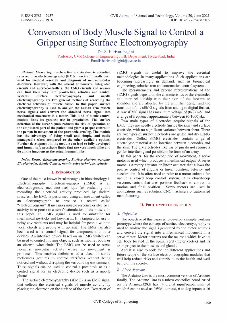
E-ISSN 2581 – 7957 CVR Journal of Science and Technology, Volume 20, June 2021 P-ISSN 2277 – 3916 DOI: 10.32377/cvrjst2016
CVR College of Engineering
Conversion of Body Muscle Signal to Control a Gripper using Surface Electromyography
Dr. S. Harivardhagini Professor, CVR College of Engineering / EIE Department, Hyderabad, India
Email: [email protected]
Abstract: Measuring muscle activation via electric potential, referred to as electromyography (EMG), has traditionally been used for medical research and diagnosis of neuromuscular disorders. However, with the advent of powerful integrated circuits and micro-controllers, the EMG circuits and sensors can find their way into prosthetics, robotics and control systems. Surface electromyography and needle electromyography are two general methods of recording the electrical activities of muscle tissue. In this paper, surface electromyography is used to analyse the human arm muscle nerve signals and convert the obtained nerve signal into mechanical movement in a motor. This kind of bionic control module finds its greatest use in prosthetics. The surface detection of the nerve signals reduces the risk of operation on the amputated part of the patient and gives a proper control to the person in movement of the prosthetic arm/leg. The module has the advantage of being small and simple, and easily manageable when compared to the other available options. Further development in the module can lead to fully developed and human safe prosthetic limbs that are very much alike and do all the functions as the actual human limbs.
Index Terms: Electromyography, Surface electromyography, Bio electrodes, Bionic Control, non-invasive technique, aphasia
I. INTRODUCTION
One of the most known breakthroughs in biotechnology is Electromyography. Electromyography (EMG) is an electrodiagnostic medicine technique for evaluating and recording the electrical activity produced by skeletal muscles. The EMG is performed using an instrument called an electromyograph to produce a record called “electromyogram”. It measures muscle response or electrical activity in response to a nerve's stimulation of the muscle. In this paper, an EMG signal is used to substitute for mechanical joysticks and keyboards. It is targeted for use in noisy environments and may be helpful for people without vocal chords and people with aphasia. The EMG has also been used as a control signal for computers and other devices. An interface device based on an EMG Switch can be used to control moving objects, such as mobile robots or an electric wheelchair. The EMG can be used to sense isometric muscular activity where no movement is produced. This enables definition of a class of subtle motionless gestures to control interfaces without being noticed and without disrupting the surrounding environment. These signals can be used to control a prosthesis or as a control signal for an electronic device such as a mobile phone.
The surface electromyography (sEMG) is an EMG signal that collects the electrical signals of muscle activity by placing the electrode on the surface of the skin. Detection of
sEMG signals is useful to improve the essential methodologies in many applications. Such applications are becoming increasingly in demand, such as biomedical engineering, robotics arm and automation control systems.
The measurements and precise representations of the sEMG signals depend on the characteristics of the electrodes and their relationship with their skin of the forearm or shoulder and are affected by the amplifier design and the transition of the sEMG signals from analog to digital format. A raw sEMG signal has maximum voltage of (0-2) mV, and a range of frequency approximately between (0-1000)Hz.
Two main types of electrodes acquire signals of the EMG; they are needle electrode (inside the skin) and surface electrode, with no significant variance between them. There are two types of surface electrodes are gelled and dry sEMG electrodes. Gelled sEMG electrodes contain a gelled electrolytic material as an interface between electrodes and the skin. The dry electrodes like bar or pin do not require a gel for interfacing and possible to be form of an array.
In this paper, for the recognition of movement, a servo motor is used which produces a mechanical output. A servo motor is a rotary actuator or linear actuator that allows the precise control of angular or linear position, velocity and acceleration. It is often used to refer to a motor suitable for use in a closed loop control system. It is closed-loop servomechanism that uses position feedback to control its motion and final position. Servo motors are used in applications such as robotics, CNC machinery or automated manufacturing.
II. PROTOTYPE CONSTRUCTION
A. Objective The objective of this paper is to develop a simple working
prototype where the concept of surface electromyography is used to analyse the signals generated by the motor neurons and convert the signal into a mechanical movement in a servo motor. Motor neurons are the neurons which have its cell body located in the spinal cord (motor cortex) and its axon project to the muscles and glands.
And it is also to look for the different applications and future scope of the surface electromyographic modules that will help reduce risks and contribute to the health and well being of the society.
B. Block diagram The Arduino Uno is the most common version of Arduino
family. The Arduino Uno is a micro controller board based on the ATmega328.It has 14 digital input/output pins (of which 6 can be used as PWM outputs), 6 analog inputs, a 16

E-ISSN 2581 – 7957 CVR Journal of Science and Technology, Volume 20, June 2021 P-ISSN 2277 – 3916 DOI: 10.32377/cvrjst2016
CVR College of Engineering
MHz ceramic resonator, a USB connection, a power jack, an ICSP header, and a reset button.
Figure 1 shows the block diagram of Bionic Control.
Figure 1. Block diagram of Bionic Control Using Electromyography The signals from human body are detected by an EMG
sensor. There are three electrodes used to sense the signals from different parts of the arm. The Arduino helps to obtain the signal and transfer to a microcontroller. The signal from the microcontroller is used to drive a motor. The whole set up uses a power supply for its functioning. The digital display is also obtained on a monitor. It is an Easy-to-use controller that detects muscle activity.
C. Circuit connections The implementation of the process has different levels or
stages. The first stage is sensing or getting the input variable to be measured and processed, then the signal is conditioned by a signal conditioning circuit that contains amplifiers, rectifiers, filters and the smootheners, a signal processing [1] happens were the signal is analyzed and then manipulated and finally an output is shown in terms of mechanical movement. Figure 2 shows the circuit connections to be taken from a human arm.
Figure 2. Circuit connections taken from an arm
The flow chart shown in figure 3 shows the stages of the signal processing done in the system.
Figure 3. Flow chart of signal processing
D. Sensing or Signal acquisition Surface EMG electrodes provide non-invasive technique for measurement and detection of EMG signal. The theory behind these electrodes is that they form a chemical equilibrium between the detecting surface and the skin of the body through electrolytic conduction, so that current can flow into the electrode. The sensors used in the circuit are the Ag-AgCl electrodes because they are more suitable for signal acquisition in Surface Electromyography. The human body is electrically neutral; it has the same number of positive and negative charges. But in the resting state, the nerve cell membrane is polarized due to differences in the concentrations and ionic composition across the plasma membrane. A potential difference exists between the intra-cellular and extra-cellular fluids of the cell. In response to a stimulus from the neuron, a muscle fiber depolarizes as the signal propagates along its surface and the fiber twitches. This depolarization, accompanied by a movement of ions, generates an electric field near each muscle fiber. An EMG signal is the train of Motor Unit Action Potential (MUAP) showing the muscle response to neural stimulation. There are three electrodes that sense and generate an electrical disturbance is the circuit, the mid muscle electrode, the end muscle electrode, and the reference electrode. The reference electrode is placed on an electrically neutral muscle and the other two electrodes are placed on the detection surface. Figure 4 shows the different types of electrodes used in this prototype.
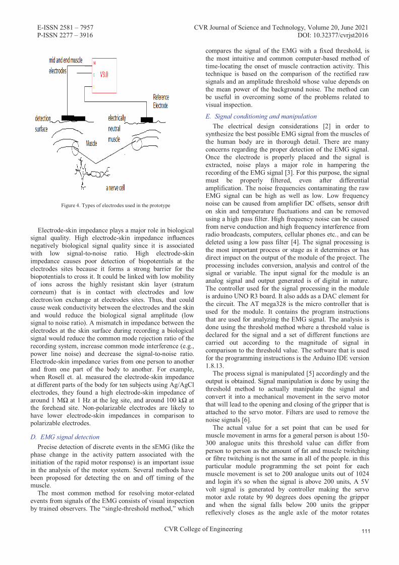
E-ISSN 2581 – 7957 CVR Journal of Science and Technology, Volume 20, June 2021 P-ISSN 2277 – 3916 DOI: 10.32377/cvrjst2016
CVR College of Engineering
Figure 4. Types of electrodes used in the prototype
Electrode-skin impedance plays a major role in biological signal quality. High electrode-skin impedance influences negatively biological signal quality since it is associated with low signal-to-noise ratio. High electrode-skin impedance causes poor detection of biopotentials at the electrodes sites because it forms a strong barrier for the biopotentials to cross it. It could be linked with low mobility of ions across the highly resistant skin layer (stratum corneum) that is in contact with electrodes and low electron/ion exchange at electrodes sites. Thus, that could cause weak conductivity between the electrodes and the skin and would reduce the biological signal amplitude (low signal to noise ratio). A mismatch in impedance between the electrodes at the skin surface during recording a biological signal would reduce the common mode rejection ratio of the recording system, increase common mode interference (e.g., power line noise) and decrease the signal-to-noise ratio. Electrode-skin impedance varies from one person to another and from one part of the body to another. For example, when Rosell et. al. measured the electrode-skin impedance at different parts of the body for ten subjects using Ag/AgCl electrodes, they found a high electrode-skin impedance of around 1 MΩ at 1 Hz at the leg site, and around 100 kΩ at the forehead site. Non-polarizable electrodes are likely to have lower electrode-skin impedances in comparison to polarizable electrodes.
D. EMG signal detection Precise detection of discrete events in the sEMG (like the
phase change in the activity pattern associated with the initiation of the rapid motor response) is an important issue in the analysis of the motor system. Several methods have been proposed for detecting the on and off timing of the muscle.
The most common method for resolving motor-related events from signals of the EMG consists of visual inspection by trained observers. The “single-threshold method,” which
compares the signal of the EMG with a fixed threshold, is the most intuitive and common computer-based method of time-locating the onset of muscle contraction activity. This technique is based on the comparison of the rectified raw signals and an amplitude threshold whose value depends on the mean power of the background noise. The method can be useful in overcoming some of the problems related to visual inspection.
E. Signal conditioning and manipulation The electrical design considerations [2] in order to
synthesize the best possible EMG signal from the muscles of the human body are in thorough detail. There are many concerns regarding the proper detection of the EMG signal. Once the electrode is properly placed and the signal is extracted, noise plays a major role in hampering the recording of the EMG signal [3]. For this purpose, the signal must be properly filtered, even after differential amplification. The noise frequencies contaminating the raw EMG signal can be high as well as low. Low frequency noise can be caused from amplifier DC offsets, sensor drift on skin and temperature fluctuations and can be removed using a high pass filter. High frequency noise can be caused from nerve conduction and high frequency interference from radio broadcasts, computers, cellular phones etc., and can be deleted using a low pass filter [4]. The signal processing is the most important process or stage as it determines or has direct impact on the output of the module of the project. The processing includes conversion, analysis and control of the signal or variable. The input signal for the module is an analog signal and output generated is of digital in nature. The controller used for the signal processing in the module is arduino UNO R3 board. It also adds as a DAC element for the circuit. The AT mega328 is the micro controller that is used for the module. It contains the program instructions that are used for analyzing the EMG signal. The analysis is done using the threshold method where a threshold value is declared for the signal and a set of different functions are carried out according to the magnitude of signal in comparison to the threshold value. The software that is used for the programming instructions is the Arduino IDE version 1.8.13.
The process signal is manipulated [5] accordingly and the output is obtained. Signal manipulation is done by using the threshold method to actually manipulate the signal and convert it into a mechanical movement in the servo motor that will lead to the opening and closing of the gripper that is attached to the servo motor. Filters are used to remove the noise signals [6].
The actual value for a set point that can be used for muscle movement in arms for a general person is about 150-300 analogue units this threshold value can differ from person to person as the amount of fat and muscle twitching or fibre twitching is not the same in all of the people. in this particular module programming the set point for each muscle movement is set to 200 analogue units out of 1024 and login it's so when the signal is above 200 units, A 5V volt signal is generated by controller making the servo motor axle rotate by 90 degrees does opening the gripper and when the signal falls below 200 units the gripper reflexively closes as the angle axle of the motor rotates
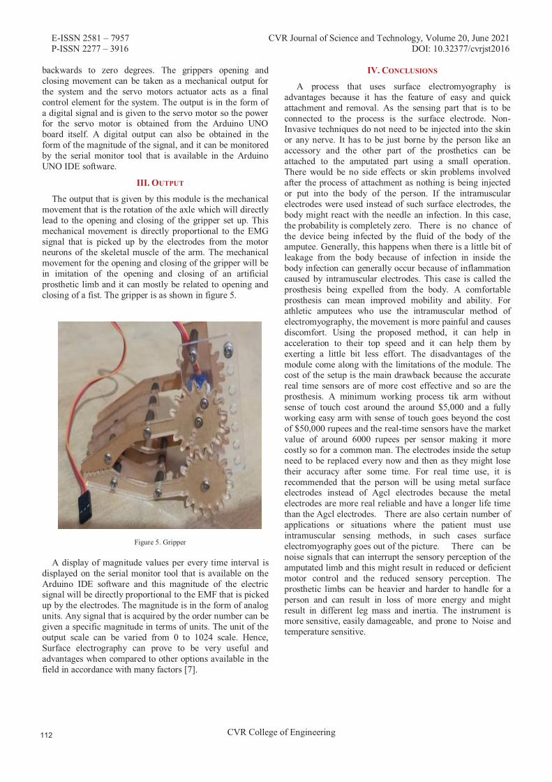
E-ISSN 2581 – 7957 CVR Journal of Science and Technology, Volume 20, June 2021 P-ISSN 2277 – 3916 DOI: 10.32377/cvrjst2016
CVR College of Engineering
backwards to zero degrees. The grippers opening and closing movement can be taken as a mechanical output for the system and the servo motors actuator acts as a final control element for the system. The output is in the form of a digital signal and is given to the servo motor so the power for the servo motor is obtained from the Arduino UNO board itself. A digital output can also be obtained in the form of the magnitude of the signal, and it can be monitored by the serial monitor tool that is available in the Arduino UNO IDE software.
III. OUTPUT
The output that is given by this module is the mechanical movement that is the rotation of the axle which will directly lead to the opening and closing of the gripper set up. This mechanical movement is directly proportional to the EMG signal that is picked up by the electrodes from the motor neurons of the skeletal muscle of the arm. The mechanical movement for the opening and closing of the gripper will be in imitation of the opening and closing of an artificial prosthetic limb and it can mostly be related to opening and closing of a fist. The gripper is as shown in figure 5.
Figure 5. Gripper A display of magnitude values per every time interval is
displayed on the serial monitor tool that is available on the Arduino IDE software and this magnitude of the electric signal will be directly proportional to the EMF that is picked up by the electrodes. The magnitude is in the form of analog units. Any signal that is acquired by the order number can be given a specific magnitude in terms of units. The unit of the output scale can be varied from 0 to 1024 scale. Hence, Surface electrography can prove to be very useful and advantages when compared to other options available in the field in accordance with many factors [7].
IV. CONCLUSIONS
A process that uses surface electromyography is advantages because it has the feature of easy and quick attachment and removal. As the sensing part that is to be connected to the process is the surface electrode. Non- Invasive techniques do not need to be injected into the skin or any nerve. It has to be just borne by the person like an accessory and the other part of the prosthetics can be attached to the amputated part using a small operation. There would be no side effects or skin problems involved after the process of attachment as nothing is being injected or put into the body of the person. If the intramuscular electrodes were used instead of such surface electrodes, the body might react with the needle an infection. In this case, the probability is completely zero. There is no chance of the device being infected by the fluid of the body of the amputee. Generally, this happens when there is a little bit of leakage from the body because of infection in inside the body infection can generally occur because of inflammation caused by intramuscular electrodes. This case is called the prosthesis being expelled from the body. A comfortable prosthesis can mean improved mobility and ability. For athletic amputees who use the intramuscular method of electromyography, the movement is more painful and causes discomfort. Using the proposed method, it can help in acceleration to their top speed and it can help them by exerting a little bit less effort. The disadvantages of the module come along with the limitations of the module. The cost of the setup is the main drawback because the accurate real time sensors are of more cost effective and so are the prosthesis. A minimum working process tik arm without sense of touch cost around the around $5,000 and a fully working easy arm with sense of touch goes beyond the cost of $50,000 rupees and the real-time sensors have the market value of around 6000 rupees per sensor making it more costly so for a common man. The electrodes inside the setup need to be replaced every now and then as they might lose their accuracy after some time. For real time use, it is recommended that the person will be using metal surface electrodes instead of Agcl electrodes because the metal electrodes are more real reliable and have a longer life time than the Agcl electrodes. There are also certain number of applications or situations where the patient must use intramuscular sensing methods, in such cases surface electromyography goes out of the picture. There can be noise signals that can interrupt the sensory perception of the amputated limb and this might result in reduced or deficient motor control and the reduced sensory perception. The prosthetic limbs can be heavier and harder to handle for a person and can result in loss of more energy and might result in different leg mass and inertia. The instrument is more sensitive, easily damageable, and prone to Noise and temperature sensitive.

E-ISSN 2581 – 7957 CVR Journal of Science and Technology, Volume 20, June 2021 P-ISSN 2277 – 3916 DOI: 10.32377/cvrjst2016
CVR College of Engineering
REFERENCES [1] G M. B. I. Raez, M.S. Hussain, and M. Yasin, “Techniques of
EMG signal analysis: detection, processing, classification and applications”, Biological Procedures Online, vol. 8, pp. 11–35, 2006.
[2] Sundaraj, K., “Cheap In-House Setup for EMG Acquisition,” IFMBE Proceedings BIOMED, pp. 146-148, 2008
[3] Surface Electromyography: Detection and Recording,” DelSys Incorporated, 1996..
[4] S.W. Johnson, P.A. Lynn, J.S.G. Miller, and G.A.L. Reed, “Miniature skin-mounted preamplifier for measurement of surface electromyographic potentials,” Medical and Biological Engineering and Computing, vol. 15, pp. 710-711, 1977.
[5] R. Merletti and H.J. Hermens, “Detection and conditioning of surface the EMG signal,” in Electromyography: physiology, engineering, and noninvasive applications, R. Merletti, and P.A. Parker, Eds. Wiley- IEEE, 2004, pp. 107-132.
[6] R.G.T. Mello, L.F. Oliveira, and J. Nadal, “Digital Butterworth filter for subtracting noise from low magnitude surface electromyogram”, Computer Methods and Programs in Biomedicine, vol. 87, pp. 28-35, 2007.
[7] M.J. Zwarts, G. Drost, and D.F. Stegeman, “Recent progress in the diagnostic use of surface EMG for neurological diseases,” Journal of Electromyography and Kinesiology, vol. 10, pp. 287-291, 2000.

E-ISSN 2581 – 7957 CVR Journal of Science and Technology, Volume 20, June 2021 P-ISSN 2277 – 3916 DOI: 10.32377/cvrjst2017
CVR College of Engineering
Examination of Specific Gravity of Urine Related to Chronic Kidney Diseases Based on MEMS and
Data Mining Dr. Narendra B. Mustare
1Professor, CVR College of Engineering/EIE Department, Hyderabad, India. Email: [email protected]
Abstract: Chronic Kidney Disease (CKD) is a major public health problem with growing challenges for its early diagnosis, timely prevention and effective treatment. The examination of specific gravity of urine in respect to CKD, like nephropathy and the parenchymal lesion is of great clinical importance for the treatment of the patient. The diagnosis of the doctor is based on accurate results in respect of the status of the specific gravity of urine. Mems is an effective and accurate tool for the measurement of the specific gravity of the liquid and thus the simulated results of the Mems are of importance in respect to the CKD mentioned above. The trend of the diseases can be correlated with the simulated output for which classification is done in the data mining software DTREG for helping the physicians so that they can prescribe the treatment of the subject in a precise manner.
Index Terms: CKD, Specific gravity of urine, MEMS and data mining.
I. INTRODUCTION
Nephropathy issues within the Udhanam region of Srikakulam district, Andhra Pradesh in India, have intended researchers to examine the assorted factors associated with kidney Diseases. Here, huge amount of farmers in agronomy are affected by Chronic Kidney Disease (CKD) [1]. It has been observed that the majority of people who are affected by this kidney disease in the Uddanam region are agricultural workers. In 2013, this CKD of the Uddanam region was named Uddanam nephropathy at the International Congress of Nephrology in China. The previous studies report states that there is a relationship between alteration of the gut microbiome (biological factor) and renal failure [2]. The Kidney is a very important regulator of equilibrium by filtration, organic process, secretion, synthesis, and degradation of metabolites in numerous pathways. Chronic means long-lasting, and CKD has been outlined based on the presence of kidney harm and its structure or faded kidney function or kidney damage and diminished function that lasts longer than three months. CKD is a serious public health issue with a universal prevalence of 13.4% and a mortality rate of 1.2 million (approx.) per year [3]. Chronic Kidney Disease (CKD) may be a worldwide health concern rising at a really quick pace. According to the National Kidney Foundation, one-tenth of the overall world population is affected by CKD leading to an increased death rate. It is estimated that in developing countries like China and India, the cases of kidney failure will increase disproportionately since the number of elderly
people is increasing due to enhanced life span [4]. Chronic Kidney Disease is also termed end-stage renal disease.
So, for the diagnosis of CKD diseases like nephropathy and parenchymal lesion, it is necessary to examine and thereby measure the specific gravity of urine [5]. The prevailing approaches of measuring the specific gravity of urine are time-consuming and involve the chances of human error. Modern techniques are needed to stop the pathogens which are responsible for CKD. With the help of various engineering techniques, one can easily design controllers to assess as well as to prevent CKD permanently. A large amount of work has been done in medical sciences in the area of CKD, but there is still scope for further research. From the recent studies, advanced tools such as data mining, etc., are considered to be the current trend in the area of CKD.
In this paper, we have introduced a new method to measure the specific gravity of urine using MEMS. The principle of a cavity resonator is being used in our method [6]. The specific gravity of the urine (i.e., the concentration of solute in urine) is measured by the Micro–Electro Mechanical System (MEMS). For minimum specific gravity, the electrodes of MEMS will vibrate with maximum amplitude and thus the amplitude of the vibration of the electrode is functionally related to specific gravity which is the underlying principle of MEMS. In specific gravity methodology, the higher the specific gravity of the fluid, the lower the resonant frequency of the filled tube. The specific gravity sensor contains a chip level, vacuum prepacked, and resonant semiconducting material tube. Whereas the tube, filled with a fluid, is driven into resonance electrostatically and its motion detected capacitively. Data obtained from the sensor is fed to software for further examination of blood samples [7].
II. RELATED WORK
In the recent past, various methods, as well as their applications, have been developed to predict CKD. In what follows, we will review and investigate related works on classification methodologies for kidney diagnosis done previously.
In the field of medical diagnosis of chronic kidney disease, D. Noia et al. presented a classifier based on the ensemble of ten artificial neural networks with the data collected over a period of 38 years [8]. A software tool has been developed predicting the end-stage kidney disease
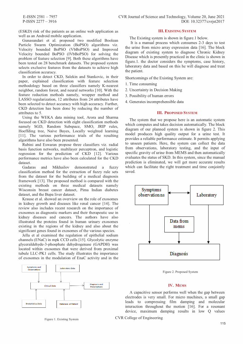
E-ISSN 2581 – 7957 CVR Journal of Science and Technology, Volume 20, June 2021 P-ISSN 2277 – 3916 DOI: 10.32377/cvrjst2017
CVR College of Engineering
(ESKD) risk of the patients as an online web application as well as an Android mobile application.
Gunasundari et al. proposed two modified Boolean Particle Swarm Optimization (BoPSO) algorithms viz. Velocity bounded BoPSO (VbBoPSO) and Improved Velocity bounded BoPSO (IVbBoPSO) for solving the problem of feature selection [9]. Both these algorithms have been tested on 28 benchmark datasets. The proposed system selects exclusive features from the datasets to achieve high classification accuracy.
In order to detect CKD, Salekin and Stankovic, in their paper, explained classification with feature selection methodology based on three classifiers namely K-nearest neighbor, random forest, and neural networks [10]. With the feature reduction methods namely, wrapper method and LASSO regularization, 12 attributes from 24 attributes have been selected to detect accuracy with high accuracy. Further, CKD detection has been done by reducing the number of attributes to 5.
Using the WEKA data mining tool, Arora and Sharma focused on CKD detection with eight classification methods namely SGD, Random Subspace, SMO, JRIP rules, Hoeffding tree, Naive Bayes, Locally weighted learning [11]. The various performance trials of the resulting algorithms have also been presented.
Rubini and Eswaran propose three classifiers viz. radial basis function networks, multilayer perceptron, and logistic regression for the prediction of CKD [12]. Various performance metrics have also been calculated for the CKD dataset.
Gadaras and Mikhailov demonstrated a fuzzy classification method for the extraction of fuzzy rule sets from the dataset for the building of a medical diagnosis framework [13]. The proposed method is compared with the existing methods on three medical datasets namely Wisconsin breast cancer dataset, Pima Indian diabetes dataset, and the Bupa liver dataset.
Krause et al. showed an overview on the role of exosomes in kidney growth and diseases like renal cancer [14]. The review also includes recent research on the importance of exosomes as diagnostic markers and their therapeutic use in kidney diseases and cancers. The authors have also illustrated the proteins found in human urinary exosomes existing in the regions of the kidney and also about the significant genes found in exosomes of the various species.
Jella et al examined the regulation of epithelial sodium channels (ENaC) in mpk CCD cells [15]. Glycolytic enzyme glyceraldehyde-3-phosphate dehydrogenase (GAPDH) was located within exosomes that were derived from proximal tubule LLC-PK1 cells. The study illustrates the importance of exosomes in the modulation of EnaC activity and in the collection of duct cells.
III. EXISTING SYSTEM
The Existing system is shown in figure.1 below. It is a manual process which consumes 2-3 days to test
the urine from micro array expression data [16]. The block diagram of existing system to diagnose Chronic Kidney Disease which is presently practiced in the clinic is shown in figure.1. the doctor considers the symptoms, case history, laboratory data and based on this he will diagnose and treat the patient.
Shortcomings of the Existing System are: 1. Time consuming 2. Uncertainty in Decision Making 3. Possibility of human errors 4. Generates incomprehensible data
III. PROPOSED SYSTEM
The system that we propose here is an automatic system which computes and takes decision automatically. The block diagram of our planned system is shown in figure 2. This model produces high quality output for a urine test. It provides a reliable performance estimate. It permits applying to unseen patients. Here, the system can collect the data from observations, laboratory testing, and the input of specific gravity of urine from MEMS and then automatically evaluates the status of SKD. In this system, since the manual prediction is eliminated, we will get more accurate results which can facilitate the right treatment and time conjointly saved.
Figure 2. Proposed System
IV. MEMS
A capacitive sensor performs well when the gap between electrodes is very small. For micro machines, a small gap leads to compressing film damping and molecular interaction throughout the motion [16]. For a resonant device, maximum damping results in low Q values
Figure 1. Existing System
E-ISSN 2581 – 7957 CVR Journal of Science and Technology, Volume 20, June 2021 P-ISSN 2277 – 3916 DOI: 10.32377/cvrjst2017
CVR College of Engineering
(resonator quality factor) or poor signal/noise ratio. Vacuum packaging of the microtube is utilized to overcome this problem along with a compatible electrical load transfer design. This has been accomplished using vacuum wafer-to-wafer bonding techniques. From MEMS, measurement of specific gravity of urine is done by examining its value with typical curve obtained within the simulation of sensor[17].
A. Relation of frequency of vibration of electrode of Mems and gain.
For minimum specific gravity, the electrodes of MEMS will vibrate with maximum amplitude which is shown in figure 3. But, the amplitude of the vibration of the electrode is functionally related to specific gravity which is the underlying principle of MEMS [18]. Both these phenomena have been simulated by MATLAB 7.0. Different curves of various resonant frequencies representing different urine samples have been simulated in MATLAB. Data obtained from MATLAB are decoded so that it can be fed to software for further examination and correlation with the data of blood samples obtained from the laboratory corresponding to the status of the subject.
Figure 3. Relation of frequency Vs gain
B. Relation of specific gravity of liquid and output voltage of Mems
As the specific gravity of the liquid increases, the density of the liquid also increases, and thus the mass of the liquid increases [19]. With different specific gravity i.e., different concentrations of liquid, the output voltage of Mems will vary according to the curve shown in figure 4.
Figure 4. Relation of specific gravity of liquid Vs output of MEMS
C. Relation of frequency and Δf
Different curves of various resonant frequencies representing different urine samples have been simulated in MATLAB. A relation between frequency(resonant frequencies) and Δf (urine samples) has been plotted after studying different curves. The relation obtained is as shown in figure 5.
Figure 5. Relation of resonant frequency(f) Vs urine samples(Δf)
D. Relation of mass of the urine (Sp. gravity) and resonant frequency
The relation of mass of the urine (Sp. Gravity) and resonant frequency is obtained using MATLAB and is shown in figure 6.
Figure 6. Relation of mass of the liquid and resonant frequency
E. MATLAB simulation for renal disorder:
The curves have been simulated in MATLAB Simulink 7.0. In this, we have simulated the curves related to the specific gravity of the urine linked to bacterial infection and this simulation is in agreement with the clinical values [20]. We have simulated the curves in a normalized way for projecting the status of the subject suffering from repeated bacterial infection. There is a possibility of renal failure with a repeated and very late bacterial infection.
A typical block diagram involved in Simulink 7.0 is shown in figure 7.
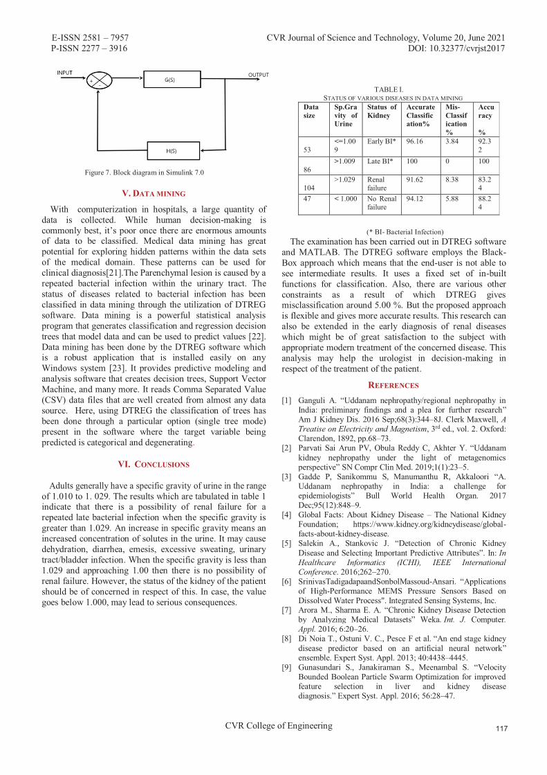
E-ISSN 2581 – 7957 CVR Journal of Science and Technology, Volume 20, June 2021 P-ISSN 2277 – 3916 DOI: 10.32377/cvrjst2017
CVR College of Engineering
Figure 7. Block diagram in Simulink 7.0
V. DATA MINING
With computerization in hospitals, a large quantity of data is collected. While human decision-making is commonly best, it’s poor once there are enormous amounts of data to be classified. Medical data mining has great potential for exploring hidden patterns within the data sets of the medical domain. These patterns can be used for clinical diagnosis[21].The Parenchymal lesion is caused by a repeated bacterial infection within the urinary tract. The status of diseases related to bacterial infection has been classified in data mining through the utilization of DTREG software. Data mining is a powerful statistical analysis program that generates classification and regression decision trees that model data and can be used to predict values [22]. Data mining has been done by the DTREG software which is a robust application that is installed easily on any Windows system [23]. It provides predictive modeling and analysis software that creates decision trees, Support Vector Machine, and many more. It reads Comma Separated Value (CSV) data files that are well created from almost any data source. Here, using DTREG the classification of trees has been done through a particular option (single tree mode) present in the software where the target variable being predicted is categorical and degenerating.
VI. CONCLUSIONS
Adults generally have a specific gravity of urine in the range of 1.010 to 1. 029. The results which are tabulated in table 1 indicate that there is a possibility of renal failure for a repeated late bacterial infection when the specific gravity is greater than 1.029. An increase in specific gravity means an increased concentration of solutes in the urine. It may cause dehydration, diarrhea, emesis, excessive sweating, urinary tract/bladder infection. When the specific gravity is less than 1.029 and approaching 1.00 then there is no possibility of renal failure. However, the status of the kidney of the patient should be of concerned in respect of this. In case, the value goes below 1.000, may lead to serious consequences.
TABLE I. STATUS OF VARIOUS DISEASES IN DATA MINING
Data size
Sp.Gravity of Urine
Status of Kidney
Accurate Classification%
Mis-Classification%
Accuracy
%
53 <=1.009
Early BI* 96.16 3.84 92.32
86 >1.009 Late BI* 100 0 100
104 >1.029 Renal
failure 91.62 8.38 83.2
4 47 < 1.000 No Renal
failure 94.12 5.88 88.2
4
(* BI- Bacterial Infection) The examination has been carried out in DTREG software and MATLAB. The DTREG software employs the Black-Box approach which means that the end-user is not able to see intermediate results. It uses a fixed set of in-built functions for classification. Also, there are various other constraints as a result of which DTREG gives misclassification around 5.00 %. But the proposed approach is flexible and gives more accurate results. This research can also be extended in the early diagnosis of renal diseases which might be of great satisfaction to the subject with appropriate modern treatment of the concerned disease. This analysis may help the urologist in decision-making in respect of the treatment of the patient.
REFERENCES [1] Ganguli A. “Uddanam nephropathy/regional nephropathy in
India: preliminary findings and a plea for further research” Am J Kidney Dis. 2016 Sep;68(3):344–8J. Clerk Maxwell, A Treatise on Electricity and Magnetism, 3rd ed., vol. 2. Oxford: Clarendon, 1892, pp.68–73.
[2] Parvati Sai Arun PV, Obula Reddy C, Akhter Y. “Uddanam kidney nephropathy under the light of metagenomics perspective” SN Compr Clin Med. 2019;1(1):23–5.
[3] Gadde P, Sanikommu S, Manumanthu R, Akkaloori “A. Uddanam nephropathy in India: a challenge for epidemiologists” Bull World Health Organ. 2017 Dec;95(12):848–9.
[4] Global Facts: About Kidney Disease – The National Kidney Foundation; https://www.kidney.org/kidneydisease/global-facts-about-kidney-disease.
[5] Salekin A., Stankovic J. “Detection of Chronic Kidney Disease and Selecting Important Predictive Attributes”. In: In Healthcare Informatics (ICHI), IEEE International Conference. 2016;262–270.
[6] SrinivasTadigadapaandSonbolMassoud-Ansari. “Applications of High-Performance MEMS Pressure Sensors Based on Dissolved Water Process". Integrated Sensing Systems, Inc.
[7] Arora M., Sharma E. A. “Chronic Kidney Disease Detection by Analyzing Medical Datasets” Weka. Int. J. Computer. Appl. 2016; 6:20–26.
[8] Di Noia T., Ostuni V. C., Pesce F et al. “An end stage kidney disease predictor based on an artificial neural network” ensemble. Expert Syst. Appl. 2013; 40:4438–4445.
[9] Gunasundari S., Janakiraman S., Meenambal S. “Velocity Bounded Boolean Particle Swarm Optimization for improved feature selection in liver and kidney disease diagnosis.” Expert Syst. Appl. 2016; 56:28–47.

E-ISSN 2581 – 7957 CVR Journal of Science and Technology, Volume 20, June 2021 P-ISSN 2277 – 3916 DOI: 10.32377/cvrjst2017
CVR College of Engineering
[10] Salekin A., Stankovic J. “Detection of Chronic Kidney Disease and Selecting Important Predictive Attributes”, In Healthcare Informatics (ICHI), IEEE International Conference. 2016;262–270.
[11] Arora M., Sharma E. “A. Chronic Kidney Disease Detection by Analyzing Medical Datasets” in Weka. Int. J. Computer. Appl. 2016; 6:20–26.
[12] Rubini L. j., Eswaran P. “Generating comparative analysis of early-stage prediction of Chronic Kidney Disease” Int. J. Mod. Eng. Res. 2015; 5:49–55.
[13] Gadaras I., Mikhailov L. “An interpretable fuzzy rule-based classification methodology for medical diagnosis” Artif. Intell. Med. 2009; 47:25–41.
[14] Krause M., Samoylenko A., Vainio S. J. “Exosomes as renal inductive signals in health and disease, and their application as diagnostic markers and therapeutic agents”, Front. cell Dev. Biol. 2015;3: 65.
[15] Jella K. K., Yu L., Yue Q et al. “Exosomal GAPDH from proximal tubule cells regulate ENaC activity”, PLoS One. 2016; 11:1–20.
[16] Moyer, V. A. & Force, U. S. P. S. T. “Screening for chronic kidney disease” U.S. Preventive Services Task Force recommendation statement. Ann. Intern. Med. 157, 567–570 (2012).
[17] Most Interesting Medical MEMS and Sensor Projects. MEMS Journal, Inc. Technology. Aug 7, 2014.
[18] D. Sparks*, S. Massoud-Ansari, M. Straayer, R. Smith, R. Schneider, J. Cripe, Y. Zhang, G. Meng “A Density / Specific Gravity Meter Based on Silicon Microtube Technology (MEMS)” -Proceedings Sensors Expo, Fall 2002, Boston, MA 2002
[19] NIH, “Urine specific gravity,” Medical Encyclopedia, MedlinePlus, www.nim.nih.gov/medlineplus/ency, 2002.
[20] A book by Devendra Chaturvedi, “Modelling and Simulation of Systems using MATLAB and Simulink’ CRC Press, Newyark,2002
[21] Karaganda, A. G.; A.S. Manjunath; M.A Jayaram “Application of Genetic Algorith Optimized Neural Network Connection Weighs for Medical Diagnosis of Pima Indians Diabetes” International Journal on Soft Computing (IJSC), Vol. 2, No.2, May 2011
[22] Chen T, Guestrin C. XG Boost “A Scalable Tree Boosting System”. In: Proceedings of the 22nd ACMSIGKDD International Conference on Knowledge Discovery and Data Mining. KDD’16. New York, NY, USA: ACM; 2016. p. 785–794.
[23] dRubini L. j., Eswaran P. “Generating comparative analysis of early-stage prediction of Chronic Kidney Disease” Int. J. Mod. Eng. Res. 2015; 5:49–55.

E-ISSN 2581 –7957 CVR Journal of Science and Technology, Volume 20, June 2021 P-ISSN 2277 – 3916 DOI: 10.32377/cvrjst2018
CVR College of Engineering
AI Based Predictive Model for Detection of Corona Patient
Dr. Santosh Kumar Sahoo Assoc. Professor, CVR College of Engineering/ EIE Department, Hyderabad, India
Email: [email protected]
Abstract: The proposed system can detect likelihood of the respiratory diseases, measure oxygen saturation and temperature of the patient. One of its goals is to test the patient for COVID-19 (i.e. pneumonia like symptoms). The system includes a testing stand which consists of respiratory sound recording unit, a pulse oximeter unit, an IR temperature check unit and a computer which consists of a software unit. The respiratory sound recording unit includes stethoscopes mounted inside a pillow on the testing stand which are connected to a microphone module which is further connected to the computer via an audio cable. The pulse oximeter unit includes a pulse oximeter sensor which is mounted on the right arm of the testing stand which is further connected to an Organic-LED (OLED) display, buzzer and the computer. The IR temperature check unit includes an IR temperature sensor which is mounted on the top arm of the testing stand which is further connected to an OLED display, buzzer and computer. It is to be noted that all the units can be adjusted according to
learning program i.e. COVID-19 diagnostic management system, present in the computer which is connected with all the above-mentioned parameters.
Index Terms: Corona virus, Chest X-ray Radiographs, Artificial Intelligence, Deep Learning, CT Scan image
I. INTRODUCTION
The whole world is currently facing a health crisis in the form of Novel corona virus (2019- nCoV) outbreak and every country is facing challenges such as testing, quarantining and treating people affected by corona virus. 15 Chinese public health authorities on 31st December 2019 reported Severe Acute Respiratory Syndrome (SARS) like pneumonia cases [1] of unidentified aetiology in the city of Wuhan, Hubei Province, China. It was later identified as a novel corona virus (2019-nCoV) and it was the causative agent of this outbreak, now known as corona virus disease 2019 (COVID-19). The virus, 2019-nCoV is a 20-novel strain of corona virus, not identified previously in humans. The initial outburst of COVID-19 in Wuhan spread briskly and greatly affected other parts of China [1]. The spread was so rapid that it took the shape of an epidemic in no time, with coverage in several other countries. Unlike Severe Acute Respiratory Syndrome (SARS), the range of 2019- nCoV epidemic is considerably wider. According to the European Centre for Disease Prevention and Control, more than 89,000 people globally were affected till March 2, 2020 and this number is increasing at an amazing rate, posing major hurdles for public health and the world economy.
World Health 30 Organization (WHO) has declared 2019-nCoV outbreak as a public health emergency of international concern (PHEIC) on January 30, 2020 and a three pandemic on March 11, 2020. WHO, while declaring it as pandemic on March 11, 2020 also announced COVID-19 as name for the new corona virus disease [2],[3]. This is historic, as WHO had declared merely two pandemics in the past: in 1918 for influenza and in 2009 for influenza H1N1. According to WHO, the official 5 numbers count as of March 16, 2020 is more than 167,000 cases in at least 150 countries with more than 6606 deaths worldwide. WHO has also released the Corona virus disease (COVID-19) advice for the public and it can be accessed through WHO website. COVID-19 testing involves analyzing samples to assess the current or past presence of SARS-CoV-2. The two main branches detect either the presence of the virus or of antibodies produced in response to infection. Tests for viral presence are used to diagnose individual cases and to allow public health authorities to trace and contain outbreaks [4]. Antibody tests instead, show whether an individual was affected with the disease. They are less useful for diagnosing current infections because antibodies may not develop for weeks after infection. It is used to assess disease prevalence, which aids the estimation of the infection fatality rate [5]. Using a stethoscope, the doctor may hear normal breathing sounds, decreased or absent breath sounds, and abnormal breath sounds. If the doctor is unable to understand the problem clearly, they might suggest taking an X-ray or CT Scan. Both have quite long procedures, they are slow, costly, and takes time to get the results [6]. In the case of corona virus, for most patients, COVID-19 begins and ends in their lungs, because like the flu, corona virus are respiratory diseases. Currently, the types of tests for COVID-19 are Polymerase Chain Reaction (PCR) swab test, antibody blood test and in some cases, X-ray or CT Scan is recommended too. One researcher found COVID preventive automated entry point (COPAEP) is an integrated system which incorporates a definite number of subsystems each enabling checks and/or preventive actions against the most obvious symptoms of corona virus [7]. The research when deployed at the entry point of the place of human assembly restricts the virus-infected people from entering the premise; and hence, mixing of the Covid-infected population and the
the height of the patient. The software unit includes a machine

E-ISSN 2581 –7957 CVR Journal of Science and Technology, Volume 20, June 2021 P-ISSN 2277 – 3916 DOI: 10.32377/cvrjst2018
CVR College of Engineering
fit ones can be prevented to lower the further spread of corona virus. The system includes methods for measuring the body-temperature and coughing of the entrant. Second researcher found COVID-19 kit: intelligent thermal scanning kit for testing the COVID-19 positivity and displaying real time count of positive case using IoT Support structures for positioning sensors on a physiologic tunnel for measuring physical, chemical and biological parameters of the body and to produce an action according to the measured value of the parameters [8] [9]. Third researcher found corona virus (COVID-19) diagnostic reagents kits. This research relates to nucleic acids and proteins from the COVID-19 corona virus. These nucleic acids and proteins can be used in the preparation and manufacture of vaccine formulations, diagnostic reagents, kits, etc Fourth researcher studied development of a heartbeat and temperature measuring system for remote health nursing during pandemic (COVID-19). The device is implemented for monitoring of heartbeat and body temperature of patient based on microcontroller using the fingertip sensor device and temperature sensor. There are few drawbacks in the existing diagnostic system. Thus, to overcome the problems, there is need to develop an improved, effective and efficient system. Hence the present research provides a COVID-19 diagnostic system using artificial intelligence and machine learning [10].
II. MODEL DESCRIPTION AND RESULT
The primary object of the present research is to provide Covid-19 diagnostic system using artificial intelligence and machine learning, which precisely detect likelihood of the Covid-19 [11]. Another object of the present research is to diagnose the patients for Covid-19 testing through respiratory sounds, oxygen saturation and temperature. Yet another object of the present research is to diagnose the patients with minimum contraction among healthcare providers and patients. Yet another object of the present research, is to quickly diagnose or test the patient which accelerates mass testing. Other objects, features and advantages will become apparent from detail description and appended claims to those skilled in art [12].
This work is described by way of example with reference to the following drawing where, Figure 1(A) shows covid-19 diagnostic system with a patient, where 100 denotes respiratory sound recording unit, 101 denotes computer, 102 denotes pulse oximeter unit, 103 denotes IR temperature check unit, 104 denotes testing stand, 105 denotes pillow, 106 denotes software unit / covid-19 diagnostic management system, 107 denotes audio cable. Figure 1B shows expanded view of covid-19 diagnostic system, where 100 denotes respiratory sound recording unit, 101 denotes computer, 102 denotes pulse oximeter unit, 103 denotes IR temperature check unit, 104 denotes testing stand, 105 denotes pillow, 106 denotes software unit / COVID-19 diagnostic
management system, 107 denotes audio cable, 108 denotes display unit [13]. Figure 2 demonstrates the block diagram of COVID-19 diagnostic system, where 200 denotes reset button, 201 denotes microcontroller, 202 denotes hardware code, 203 denotes stethoscope's microphone, 204 denotes pulse oximeter, 205 denotes IR temperature sensor, 206 denotes computer system, 207 denotes OLED display, 208 denotes buzzer, Figure 3 of represents the flow chart of procedure of COVID-19 diagnostic system. Figure 4 describes the final test reports (Figure 4(A), & 4(B)) generated by the Covid COVID-19 diagnostic management system [14] [15]. The manner in which the above-cited and other advantages and objects of the research are obtained, a more detailed description of the research briefly described above, will be referred to, which is illustrated in the appended drawing. Understanding that these drawings depict only typical embodiment of the research and therefore not to be considered limiting in its scope, the research will be described with additional specificity and details through the use of the accompanying drawing 6 Detailed description of research: The present research relates to COVID-19 diagnostic system using artificial intelligence and machine learning which precisely detects likelihood of the COVID-19. It comprises of a testing stand which consists of arespiratory sound recording unit, a pulse oximeter unit, an IR temperature check unit and a computer which consists of a software unit. Herein, the respiratory sound recording unit includes stethoscopes mounted inside a pillow which are connected to a microphone module which is further connected to the computer via an audio cable, the pulse oximeter unit includes a pulse oximeter sensor which is mounted on the right arm of the testing stand which is further connected to an OLED display, a buzzer and the computer and the IR temperature check unit includes an IR temperature sensor, which is mounted on the top arm of the testing stand which is further connected to an OLED display, a buzzer and the computer [16]. In this present task all the units can be adjusted according to the height of the patient. The software unit includes a machine learning program i.e. COVID-19 Diagnostic Management System, present in the computer which is connected to all the above-mentioned parameters. Here, system can detect respiratory diseases, measure oxygen saturation and temperature of the patient [17]. For recording the respiratory sound of the patient, the patient needs to stand in front of the testing stand in such a way that his back is facing the testing stand. The patient should make sure that his back is in contact with the pillow present on the testing stand. The height of the pillow can be manually adjusted according to the height and comfort of the patient. Then, the patient should take deep breaths for 30 seconds and relax. Meanwhile, the respiratory recording unit records the respiratory sounds and transmits it to the software present in the computer. For the
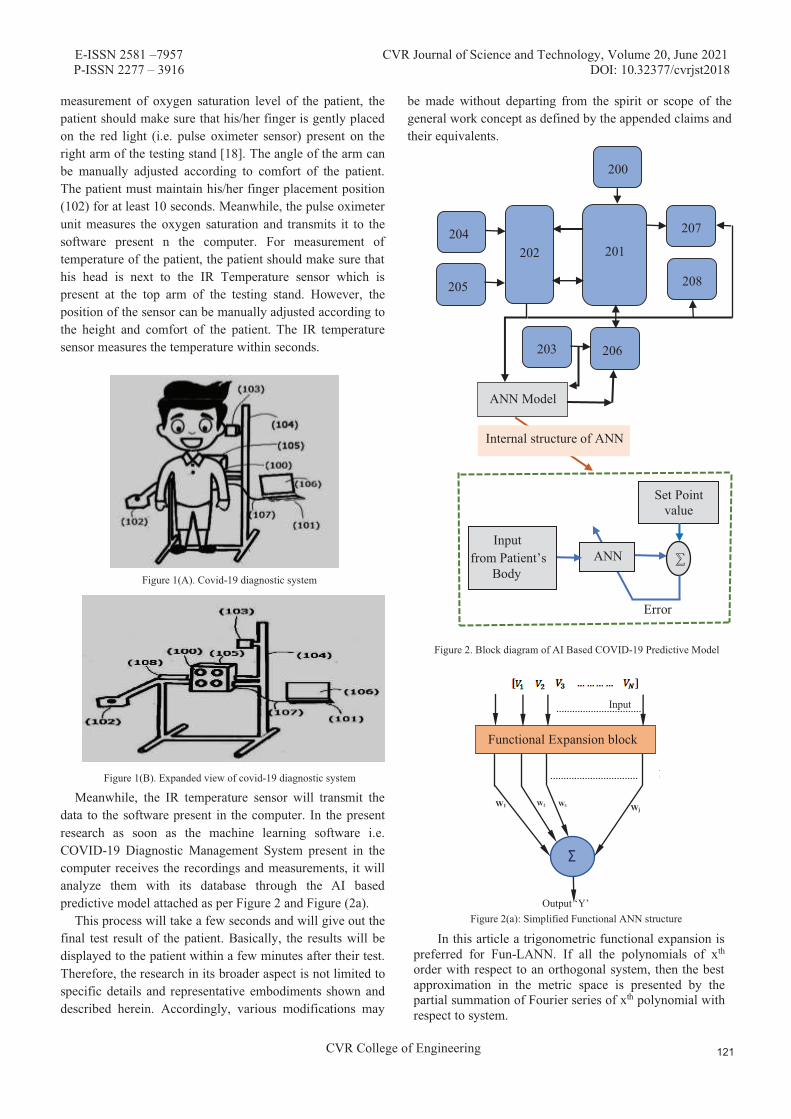
E-ISSN 2581 –7957 CVR Journal of Science and Technology, Volume 20, June 2021 P-ISSN 2277 – 3916 DOI: 10.32377/cvrjst2018
CVR College of Engineering
measurement of oxygen saturation level of the patient, the patient should make sure that his/her finger is gently placed on the red light (i.e. pulse oximeter sensor) present on the right arm of the testing stand [18]. The angle of the arm can be manually adjusted according to comfort of the patient. The patient must maintain his/her finger placement position (102) for at least 10 seconds. Meanwhile, the pulse oximeter unit measures the oxygen saturation and transmits it to the software present n the computer. For measurement of temperature of the patient, the patient should make sure that his head is next to the IR Temperature sensor which is present at the top arm of the testing stand. However, the position of the sensor can be manually adjusted according to the height and comfort of the patient. The IR temperature sensor measures the temperature within seconds.
Figure 1(A). Covid-19 diagnostic system
Figure 1(B). Expanded view of covid-19 diagnostic system
Meanwhile, the IR temperature sensor will transmit the data to the software present in the computer. In the present research as soon as the machine learning software i.e. COVID-19 Diagnostic Management System present in the computer receives the recordings and measurements, it will analyze them with its database through the AI based predictive model attached as per Figure 2 and Figure (2a).
This process will take a few seconds and will give out the final test result of the patient. Basically, the results will be displayed to the patient within a few minutes after their test. Therefore, the research in its broader aspect is not limited to specific details and representative embodiments shown and described herein. Accordingly, various modifications may
be made without departing from the spirit or scope of the general work concept as defined by the appended claims and their equivalents.
Figure 2. Block diagram of AI Based COVID-19 Predictive Model
Figure 2(a): Simplified Functional ANN structure
In this article a trigonometric functional expansion is preferred for Fun-LANN. If all the polynomials of xth order with respect to an orthogonal system, then the best approximation in the metric space is presented by the partial summation of Fourier series of xth polynomial with respect to system.
204
205
202 201
200
203 206
207
208
Internal structure of ANN
ANN Model
Error
ANN Input
from Patient’s Body
Set Point value
⅀
Output ‘Y’
W1 Wj W3 W2
Input
M
Functional Expansion block
Σ
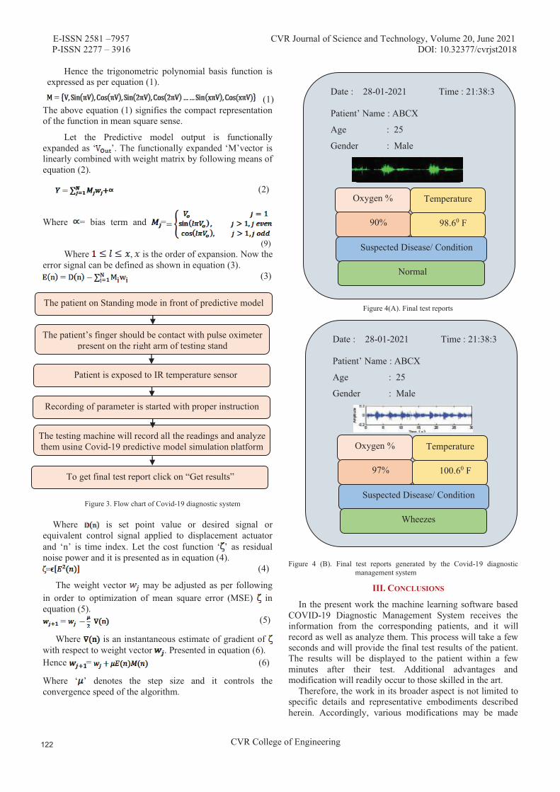
E-ISSN 2581 –7957 CVR Journal of Science and Technology, Volume 20, June 2021 P-ISSN 2277 – 3916 DOI: 10.32377/cvrjst2018
CVR College of Engineering
Hence the trigonometric polynomial basis function is expressed as per equation (1).
(1) The above equation (1) signifies the compact representation of the function in mean square sense.
Let the Predictive model output is functionally expanded as ‘ ’. The functionally expanded ‘M’vector is linearly combined with weight matrix by following means of equation (2).
(2)
Where = bias term and =
(9) Where , is the order of expansion. Now the
error signal can be defined as shown in equation (3). (3)
Figure 3. Flow chart of Covid-19 diagnostic system
Where is set point value or desired signal or equivalent control signal applied to displacement actuator and ‘n’ is time index. Let the cost function ‘ ’ as residual noise power and it is presented as in equation (4).
(4)
The weight vector may be adjusted as per following in order to optimization of mean square error (MSE) in equation (5).
(5)
Where is an instantaneous estimate of gradient of with respect to weight vector . Presented in equation (6). Hence = (6)
Where ‘ ’ denotes the step size and it controls the convergence speed of the algorithm.
Figure 4(A). Final test reports
Figure 4 (B). Final test reports generated by the Covid-19 diagnostic management system
III. CONCLUSIONS
In the present work the machine learning software based COVID-19 Diagnostic Management System receives the information from the corresponding patients, and it will record as well as analyze them. This process will take a few seconds and will provide the final test results of the patient. The results will be displayed to the patient within a few minutes after their test. Additional advantages and modification will readily occur to those skilled in the art.
Therefore, the work in its broader aspect is not limited to specific details and representative embodiments described herein. Accordingly, various modifications may be made
Date : 28-01-2021 Time : 21:38:3
Patient’ Name : ABCX
Age : 25
Gender : Male
Oxygen % Temperature
97% 100.60 F
Suspected Disease/ Condition
Wheezes
Date : 28-01-2021 Time : 21:38:3
Patient’ Name : ABCX
Age : 25
Gender : Male
Oxygen % Temperature
90% 98.60 F
Suspected Disease/ Condition
Normal
The patient on Standing mode in front of predictive model
The patient’s finger should be contact with pulse oximeter present on the right arm of testing stand
Patient is exposed to IR temperature sensor
Recording of parameter is started with proper instruction
The testing machine will record all the readings and analyze them using Covid-19 predictive model simulation platform
To get final test report click on “Get results”

E-ISSN 2581 –7957 CVR Journal of Science and Technology, Volume 20, June 2021 P-ISSN 2277 – 3916 DOI: 10.32377/cvrjst2018
CVR College of Engineering
without departing from the spirit or scope of the general research concept as defined by the appended objective and their equivalents.
REFERENCES
[1] Ruiz Estrada MA. The uses of drones in case of massive Epidemics contagious diseases relief humanitarian aid: Wuhan-COVID-19 crisis. SSRN Electron J 2020.
[2] Nguyen TT, Waurn G, Campus P. Artificial intelligence in the battle against corona virus (COVID-19): A survey and future research directions. 2020
[3] Maghdid HS, Ghafoor KZ, Sadiq AS, Curran K, Rabie K. A novel AI-enabled framework to diagnose coronavirus COVID 19 using smartphone embedded sensors: design study. 2020. page. 1-5.
[4] Wang CJ, New T, Sun F, et al. Response to COVID-19 in Taiwan big data analytics, new technology, and proactive testing. 2020. p. 1-2.
[5] Aishwarya Kumar, Puneet Kumar Gupta*, Ankita Srivastava, A review of modern technologies for tackling COVID-19 pandemic, Elsevier, Diabetes & Metabolic Syndrome: Clinical Research & Reviews 14 (2020) pg -569-573
[6] Ai T, Yang Z, Hou H, Zhan C, Chen C, Lv W, Tao Q, Sun Z, Xia L. Correlation of chest CT and RT-PCR testing in corona virus disease 2019 (COVID-19) in China: a report of 1014 cases. Radiology 2020.
[7] Luo H, Tang QL, Shang YX, Liang SB, Yang M, Robinson N, Liu JP. Can Chinese medicine be used for prevention of coronavirus disease 2019 (COVID-19)? A review of historical classics, research evidence and current prevention programs. Chin J Integr Med 2020.
[8] Haleem A, Vaishya R, Javaid M, Khan IH. Artificial Intelligence (AI) applications in orthopaedics: an innovative technology to embrace. J Clin Orthop Trauma 2019.
[9] Stebbing J, Phelan A, Griffin I, Tucker C, Oechsle O, Smith D, Richardson P. COVID-19: combining antiviral and anti-inflammatory treatments. Lancet Infect Dis 2020 Feb 27.
[10] Raju Vaishya, Mohd Javaid, Ibrahim Haleem Khan, Abid Haleem, Artificial Intelligence (AI) applications for COVID-19 pandemic, Elsevier, Diabetes & Metabolic Syndrome: Clinical Research & Reviews 14 (2020) Page 337-339
[11] Pedro R. A. S. Bassi, Romis Attux, A Deep Convolutional Neural Network for COVID-19 Detection Using Chest X-Rays, arXiv:2005.01578v2[eess.2], 18 june 2020, page – 1-19
[12] Asif Iqbal Khan, Junaid Latief Shah, Mohammad Mudasir Bhat, CoroNet: A deep neural network for detection and diagnosis of COVID-19 from chest x-ray images, Elsevier, Computer Methods and Programs in Biomedicine 196 (2020) 105581, Page 1-9
[13] Lin Li, BS Lixin Qin, PhD • Zeguo Xu, BS • Youbing Yin, PhD • Xin Wang, PhD • Bin Kong, PhD • Junjie Bai, PhD • Yi Lu, MS • Zhenghan Fang, MS • Qi Song, PhD • Kunlin Cao, PhD • Daliang Liu, PhD • Guisheng Wang, PhD • Qizhong Xu, MS • Xisheng Fang, BS • Shiqin Zhang, BS •
Juan Xia, BS • Jun Xia, PhD, Using Artificial Intelligence to Detect COVID-19 and Community-acquired Pneumonia Based on Pulmonary CT, Radiology 2020.
[14] Clinical Trials.gov. Bethesda (MD): National Library of Medicine (US). Identifier NCT03945825, Flublok or Fluzone With Advax-CpG55.2 or AF03; 2020 March 16 [cited 2020 March 23];
[15] Park A. AI develops’ turbocharged’ flu vaccine: A clinical trial will soon be underway in the U.S. to test the efficacy of an enhanced flu vaccine developed by an artificial intelligence system at Flinders University in South Australia. Becker’s Hospital Review. Accessed March 24, 2020.
[16] Smith M, Smith JC. Repurposing therapeutics for COVID-19: Supercomputer-based docking to the SARS-CoV-2 viral Spike Protein and viral spike protein-human ACE2 interface. Chem Rxiv 2020,
[17] Artificial intelligence and COVID-19: A multidisciplinary approach, Integrative Medicine Research 9 (2020) 100434
[18] Pravin RK, Akojwar SG, Bajaj ND. 2018. A hybridized neural network and optimization algorithms for prediction and classification of neurological disorders. Int J Biomed Eng Technol. 28(4):307–321.

E-ISSN 2581 – 7957 CVR Journal of Science and Technology, Volume 20, June 2021 P-ISSN 2277 – 3916 DOI: 10.32377/cvrjst2019
CVR College of Engineering
Development of an Android Application for COVID-19 using Firebase and Geo-fencing
Jannaikode Yashwanth Kumar1 and S.V. Suryanarayana2
Email: [email protected]
Email: [email protected]
Abstract: The coronavirus has challenged the lives of many people all around the globe. The widespread use of COVID-19 left people starving with no money and bread. To combat this effect on people the only way is to maintain social distance and be cautious all the time. We put forward a mobile application-based strategy to combat the risk of COVID-19. The motive of the proposed model is to make people aware of COVID-19 cases updates and also notify them at various situations. We developed the mobile application using android studio and made use of Google firebase for the database. COVID-19 cases status along with information related to pandemic and emergency contacts are featured in the application. The outcomes of the application are good in response time as well as in the delivering of notifications.
Index Terms: Geo-Fencing, Mobile Application, COVID-19, Android Studio, Google Firebase
The dreadful COVID-19 virus affected several lives all around the globe. COVID-19 pandemic has been declared a global health emergency by the World Health Organization (WHO) [1]. WHO has suggested a ‘test-isolate-trace’ approach throughout the pandemic [2]. In parallel, there has been a worldwide cooperative effort to develop a vaccine and numerous serological tests for the presence of antibodies [3]. This alarming situation has a great deal of impact on the lives of citizens. Many people across the globe are infected and have died due to this virus [4]. Strong immunity surely saves people at risk from getting affected with COVID-19. Children below 10 years and adults above 60 years are vulnerable to this disease as per the recorded statistics. Keeping ourselves clean and eating a nutritious diet would help us prevent ourselves from the deadly infection of the disease. The coronavirus has brought all the people together to strive hard in the field of science and technology so as to contribute to the society in this distressed period [5]. Since there is a rampant usage of mobile phones, every citizen has the knowledge of using mobile applications. There is no doubt in saying that mobile applications are pre-dominant than web-based applications. As the COVID-19 pandemic rages, engineers and researchers are coming up with applications, services, systems for contact tracing and many more creative ideas [6].
Mobile applications keep track of registered users so that they can know the vulnerable areas. Coronavirus Pandemic Epidemiology (COPE) has come up with a symptom tracker mobile application which collects the data and analyzes the effect of COVID-19 in different areas, thus residents in those localities can be alerted to take precautions. This application, launched in the UK, got a great reach of 2.8 million users in less than 2 months [7]. People get information regarding COVID-19 happenings around them through their mobiles. COVID-19 cases are gradually increasing irrespective of many lockdowns and strict guidelines given by the governments. The UK Government has a motive that better contact tracing application plays a vital role in beating COVID-19 and helps the present situation become new normal [8].
People can be alert all the time of what is happening around them through the updates. Mobile applications serve as a better aid to fulfill this requirement. The application developed notifies the user on entering and exiting the containment region. Many people are dubious that the virus spreads via waves. All these assumptions are absurd. Many countries, which do not have a 5G network, have a lot more COVID-19 cases than the countries which have better networks [9]. The organization of the paper is as follows. Section II of the paper deals with literature survey on applications in the market and their limitations. Section III gives better knowledge on proposed methodology. In section IV, results and performance of the application is discussed. Section V gives conclusion along with the future work of the proposed model.
II. L SURVEY
At present many applications exist all over the world, which give information related to COVID-19. In India, many states have developed an application to provide their state COVID-19 updates and information. Kerala, Tamil Nadu, Punjab, Maharashtra and Mizoram states have come up with the mobile applications for safeguarding the lives of their states’ people [10]. There are API’s which provide data regarding COVID-19 cases and updates [11]. These API’s make work easier as there is no need to update the database manually. Existing API’s provide data related to countries and states round the globe.
I. INTRODUCTION
1UG Scholar, CVR College of Engineering/IT Department, Hyderabad, India
2Assoc. Professor, CVR College of Engineering/IT Department, Hyderabad, India
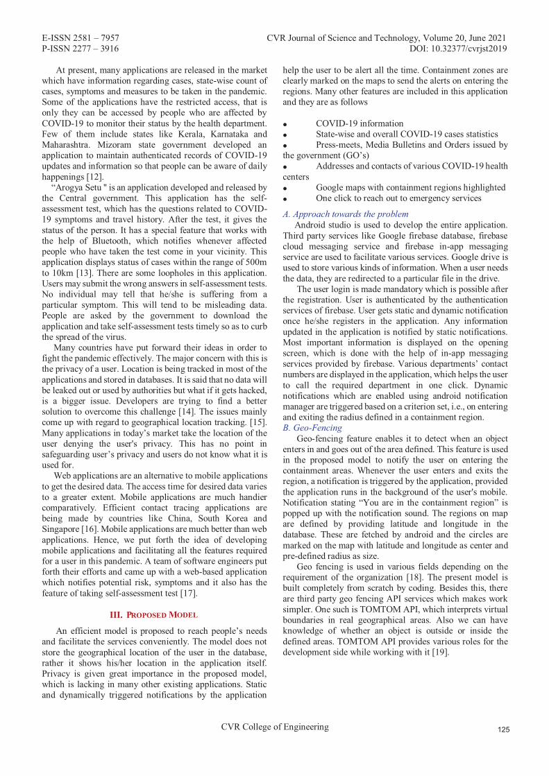
E-ISSN 2581 – 7957 CVR Journal of Science and Technology, Volume 20, June 2021 P-ISSN 2277 – 3916 DOI: 10.32377/cvrjst2019
CVR College of Engineering
At present, many applications are released in the market which have information regarding cases, state-wise count of cases, symptoms and measures to be taken in the pandemic. Some of the applications have the restricted access, that is only they can be accessed by people who are affected by COVID-19 to monitor their status by the health department. Few of them include states like Kerala, Karnataka and Maharashtra. Mizoram state government developed an application to maintain authenticated records of COVID-19 updates and information so that people can be aware of daily happenings [12]. “Arogya Setu '' is an application developed and released by the Central government. This application has the self-assessment test, which has the questions related to COVID-19 symptoms and travel history. After the test, it gives the status of the person. It has a special feature that works with the help of Bluetooth, which notifies whenever affected people who have taken the test come in your vicinity. This application displays status of cases within the range of 500m to 10km [13]. There are some loopholes in this application. Users may submit the wrong answers in self-assessment tests. No individual may tell that he/she is suffering from a particular symptom. This will tend to be misleading data. People are asked by the government to download the application and take self-assessment tests timely so as to curb the spread of the virus. Many countries have put forward their ideas in order to fight the pandemic effectively. The major concern with this is the privacy of a user. Location is being tracked in most of the applications and stored in databases. It is said that no data will be leaked out or used by authorities but what if it gets hacked, is a bigger issue. Developers are trying to find a better solution to overcome this challenge [14]. The issues mainly come up with regard to geographical location tracking. [15]. Many applications in today’s market take the location of the user denying the user's privacy. This has no point in safeguarding user’s privacy and users do not know what it is used for. Web applications are an alternative to mobile applications to get the desired data. The access time for desired data varies to a greater extent. Mobile applications are much handier comparatively. Efficient contact tracing applications are being made by countries like China, South Korea and Singapore [16]. Mobile applications are much better than web applications. Hence, we put forth the idea of developing mobile applications and facilitating all the features required for a user in this pandemic. A team of software engineers put forth their efforts and came up with a web-based application which notifies potential risk, symptoms and it also has the feature of taking self-assessment test [17].
III. P M
An efficient model is proposed to reach people’s needs and facilitate the services conveniently. The model does not store the geographical location of the user in the database, rather it shows his/her location in the application itself. Privacy is given great importance in the proposed model, which is lacking in many other existing applications. Static and dynamically triggered notifications by the application
help the user to be alert all the time. Containment zones are clearly marked on the maps to send the alerts on entering the regions. Many other features are included in this application and they are as follows � COVID-19 information � State-wise and overall COVID-19 cases statistics � Press-meets, Media Bulletins and Orders issued by the government (GO’s) � Addresses and contacts of various COVID-19 health centers � Google maps with containment regions highlighted � One click to reach out to emergency services
A. Approach towards the problem Android studio is used to develop the entire application. Third party services like Google firebase database, firebase cloud messaging service and firebase in-app messaging service are used to facilitate various services. Google drive is used to store various kinds of information. When a user needs the data, they are redirected to a particular file in the drive. The user login is made mandatory which is possible after the registration. User is authenticated by the authentication services of firebase. User gets static and dynamic notification once he/she registers in the application. Any information updated in the application is notified by static notifications. Most important information is displayed on the opening screen, which is done with the help of in-app messaging services provided by firebase. Various departments’ contact numbers are displayed in the application, which helps the user to call the required department in one click. Dynamic notifications which are enabled using android notification manager are triggered based on a criterion set, i.e., on entering and exiting the radius defined in a containment region. B. Geo-Fencing Geo-fencing feature enables it to detect when an object enters in and goes out of the area defined. This feature is used in the proposed model to notify the user on entering the containment areas. Whenever the user enters and exits the region, a notification is triggered by the application, provided the application runs in the background of the user's mobile. Notification stating “You are in the containment region” is popped up with the notification sound. The regions on map are defined by providing latitude and longitude in the database. These are fetched by android and the circles are marked on the map with latitude and longitude as center and pre-defined radius as size. Geo fencing is used in various fields depending on the requirement of the organization [18]. The present model is built completely from scratch by coding. Besides this, there are third party geo fencing API services which makes work simpler. One such is TOMTOM API, which interprets virtual boundaries in real geographical areas. Also we can have knowledge of whether an object is outside or inside the defined areas. TOMTOM API provides various roles for the development side while working with it [19].

E-ISSN 2581 – 7957 CVR Journal of Science and Technology, Volume 20, June 2021 P-ISSN 2277 – 3916 DOI: 10.32377/cvrjst2019
CVR College of Engineering
C. Implementation
Figure 1. Block diagram of application functionality
Figure 1, explains about the application functionality. The user logs in after the authentication done by google firebase authentication. User fetches data from firebase database or is redirected to corresponding google drive folders. Notifications are triggered on entering into the containment region which is facilitated using notification manager in firebase. Static notifications are enabled with the help of firebase cloud messaging service, which also helps the admin to see various analytics. In-app messaging services are also added to focus on more important issues on opening the application. Admin needs to post the required information in the site beforehand, size, banner, text and image need to be added in the site while sending these notifications.[20].
IV. R A
A. Application design and their functionality The design of the application is shown in figure 2. User login and registration pages are seen in 2.A screen and In screen 2.B, homepage consisting of information regarding COVID-19, its symptoms and preventive measures to be taken can be seen.
Figure 2. Screenshots of the application interface
Figure 3. Screenshots of containment regions and dynamic notification
Figure 3, shows the major part of the complete application. Users on entering the containment region get the notification as shown in C. User can check where he is on the map. This is illustrated clearly in screen A. B screen clearly shows all the containment regions. This helps the user to plan before travelling to a place in the vicinity of contained regions, thus making him alert by giving the knowledge of vulnerable areas.
Figure 4. Screenshots of application with different features
In figure 4, screen A displays the auto scrolling updates which are updated by the admin in the database, screen B has the list of emergency contacts through which the user can ring up but tapping on the number and giving permission to the app to make calls. Cloud messaging service is used to trigger static alerts that can be visualized in screen C. Cloud messaging service enables to send any number of notifications at any time with desired content and image [21].
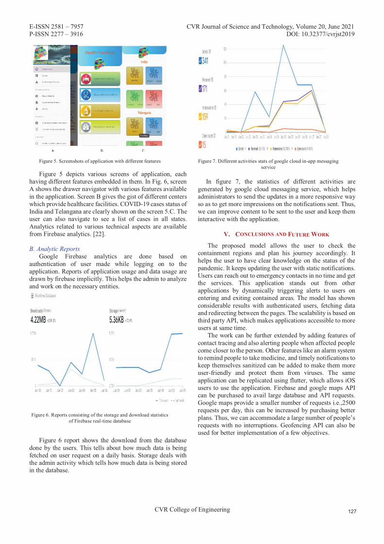
E-ISSN 2581 – 7957 CVR Journal of Science and Technology, Volume 20, June 2021 P-ISSN 2277 – 3916 DOI: 10.32377/cvrjst2019
CVR College of Engineering
Figure 5. Screenshots of application with different features
Figure 5 depicts various screens of application, each having different features embedded in them. In Fig. 6, screen A shows the drawer navigator with various features available in the application. Screen B gives the gist of different centers which provide healthcare facilities. COVID-19 cases status of India and Telangana are clearly shown on the screen 5.C. The user can also navigate to see a list of cases in all states. Analytics related to various technical aspects are available from Firebase analytics. [22]. B. Analytic Reports Google Firebase analytics are done based on authentication of user made while logging on to the application. Reports of application usage and data usage are drawn by firebase implicitly. This helps the admin to analyze and work on the necessary entities.
Figure 6. Reports consisting of the storage and download statistics of Firebase real-time database
Figure 6 report shows the download from the database done by the users. This tells about how much data is being fetched on user request on a daily basis. Storage deals with the admin activity which tells how much data is being stored in the database.
Figure 7. Different activities stats of google cloud in-app messaging service
In figure 7, the statistics of different activities are generated by google cloud messaging service, which helps administrators to send the updates in a more responsive way so as to get more impressions on the notifications sent. Thus, we can improve content to be sent to the user and keep them interactive with the application.
V. C F W
The proposed model allows the user to check the containment regions and plan his journey accordingly. It helps the user to have clear knowledge on the status of the pandemic. It keeps updating the user with static notifications. Users can reach out to emergency contacts in no time and get the services. This application stands out from other applications by dynamically triggering alerts to users on entering and exiting contained areas. The model has shown considerable results with authenticated users, fetching data and redirecting between the pages. The scalability is based on third party API, which makes applications accessible to more users at same time. The work can be further extended by adding features of contact tracing and also alerting people when affected people come closer to the person. Other features like an alarm system to remind people to take medicine, and timely notifications to keep themselves sanitized can be added to make them more user-friendly and protect them from viruses. The same application can be replicated using flutter, which allows iOS users to use the application. Firebase and google maps API can be purchased to avail large database and API requests. Google maps provide a smaller number of requests i.e.,2500 requests per day, this can be increased by purchasing better plans. Thus, we can accommodate a large number of people’s requests with no interruptions. Geofencing API can also be used for better implementation of a few objectives.

E-ISSN 2581 – 7957 CVR Journal of Science and Technology, Volume 20, June 2021 P-ISSN 2277 – 3916 DOI: 10.32377/cvrjst2019
CVR College of Engineering
[1]. COVID-19 outbreak: Migration, effects on society, global environment and prevention, https://www.sciencedirect.com/science/article/pii/S0048969720323998
[2]. BBC News, “WHO head: ‘Our key message is: test, test,test.’” https://www.bbc.co.uk/news/av/world51916707/who-head-our-key-message-is-test-test- test.
[3]. Pethick, “Developing antibody tests for SARS-CoV-2,”Lancet, vol. 395 (10230).
[4]. E. Hernández-Orallo, P. Manzoni, C. T. Calafate and J. Cano, "Evaluating How Smartphone Contact Tracing Technology Can Reduce the Spread of Infectious Diseases: The Case of COVID-19," in IEEE Access, vol. 8, pp. 99083-99097, 2020, doi: 10.1109/ACCESS.2020.2998042.
[5]. How Reliable and Effective Are the Mobile Apps Being Used to Fight COVID-19?, https://thewire.in/tech/COVID-19-mobile-apps-india
[6]. A flood of coronavirus apps are tracking us. Now it’s time tokeep track of them, https://www.technologyreview.com/2020/05/07/1000961/launching-mittr-COVID-19- tracing-tracker/
[7]. Now, a mobile app predicts COVID-19 incidence days in advance, https://www.thehindu.com/sci-tech/science/now-a-mobile-app-predicts-COVID-19-incidence-days-in-advance/article31544706.ece
[8]. COVID-19 apps around the world, https://techerati.com/features-hub/opinions/COVID-19- apps-around-the-world/
[9]. 5G mobiles do not spread COVID-19, https://www.who.int/emergencies/diseases/novel-coronavirus-2019/advice-for-public/myth-busters?gclid=Cj0KCQjwudb3BRC9ARIsAEa- vUvdlwAV59nTqxfJ1xp7nKMD9TZsiT4mksqnq11xrTuO37kL9m1qwwaAj_tEALw_wc B#5g
[10]. Coronavirus Apps: Every App the Central Government And States Have Deployed to Track COVID-19
[11]. https://gadgets.ndtv.com/apps/features/central-state-governments-launch-coronavirus- mobile-app-list-2204286
[12]. Corona virus app API,https://coronavirus.app/map?compared=US,DE,FR,GB,ES
[13]. Mizoram launches coronavirus app to disseminate authoritative info to the public https://www.deccanchronicle.com/technology/in-other-news/040420/mizoram-launches-coronavirus-app-to-disseminate-authoritative-info-to.html
[14]. Aarogya Setu- Features and tools https://en.wikipedia.org/wiki/Aarogya_Setu
[15]. Top-10 smartphone apps to track COVID- 19,https://www.geospatialworld.net/blogs/popular-apps-COVID-19
[16]. COVID-19 Apps. https://en.wikipedia.org/wiki/COVID-19_apps
[17]. COVID-19: The world embraces contact-tracing technology to fight the virushttps://www.livemint.com/news/world/COVID-19-the-world-embraces-contact-tracing-
[18]. CheckCOVID-19Now: A web app to spot coronavirus cases in Telangana,https://www.newindianexpress.com/cities/hyderabad/2020/apr/18/checkCOVID-19now-a-web-app-to-spot-coronavirus-cases-in-telangana-2131600.html
[19]. Geo-Fence ,Applications, https://en.wikipedia.org/wiki/Geo-fence
[20]. TOMTOM Geo Fencing API documentation, https://developer.tomtom.com/geofencing- api/geofencing-api-documentation
[21]. Firebase in-app messaging,https://firebase.google.com/docs/in-app-messaging/compose-campaign?authuser=2
[22]. Sending messages to multiple devices, https://firebase.google.com/docs/cloud-messaging/android/send-multiple?authuser=2
[23]. Firebase console databasehttps://firebase.google.com/docs/database/usage/monitor- usage?authuser=2
REFERENCES

E-ISSN 2581 – 7957 CVR Journal of Science and Technology, Volume 20, June 2021 P-ISSN 2277 – 3916 DOI: 10.32377/cvrjst2020
CVR College of Engineering
Design and Process Analysis of Single Cavity Injection Molding Die for Plastic Wing Nut
Neeraj Kumar Jha1, G. Bharath Reddy2 and Vidyanand Kumar3 1Assoc. Professor, CVR College of Engineering/ Mechanical Engg. Department, Hyderabad, India
Email: [email protected] 2Asst. Professor, CVR College of Engineering/ Mechanical Engg. Department, Hyderabad, India
Email: [email protected] 3Asst. Professor, CVR College of Engineering/ Mechanical Engg. Department, Hyderabad, India
Email: [email protected]
Abstract: Material selection is an important step under active planning phase in production planning and control and, so is process selection. Polymers are preferable option for various products due to their desirable properties. Light weight, low cost, corrosion resistant and high strength to weight ratio is few among them. In similar manner injection molding is the most suitable process to be preferred for processing various grades of thermoplastics. The process preferably utilizes a heating unit to take polymers to their injection temperature, a permanent mold with shaped cavity as the shape of the required product along with clamping and cooling provisions. The process is best suitable for mass production of plastic parts and is widely used industrially. The permanent mold used in injection molding process is also referred as plastic mold. These molds must be designed and analyzed before their manufacturing to ensure suitability of the molding with particular plastic material type. This article attempts to ensure suitability of molding plastic wing nuts, an internal threaded component, by injection molding process with polypropylene (PP) and high density poly ethylene (HDPE) material. Modeling of parts is done with UG Nx 9.0 while the flow analysis is performed by Autodesk Mold Flow Adviser 2015.
Index Terms: Injection molding, permanent mold, internal threaded component, polypropylene, high density poly ethylene.
I. INTRODUCTION
Injection molding is commonly used method for manufacturing of plastic components with complex geometries [1]. This process is considered as one of the primary shaping process which utilizes a permanent mold along with injection molding machine. The four phases of injection molding processes are clamping, injection, cooling and ejection [2]. Clamping is about closing the split mold and holding it to withstand injection pressure. Injection is about pressurized filling of the mold cavity with plastic material at semisolid phase. It utilizes shot volume, the volume of material sufficient to fill all the cavities of die at once. Solidification of the filled cavity by transferring temperature to the mold walls is referred as cooling. Ejection is the process of removal of solidified component from permanent mold cavity after opening of the split mold. The process is simple to observe, operate and automate but it involves proper understanding, care and analysis of numerous parameters. These parameters must be analyzed well before the die manufacturing to prevent loss of time
and money. The conventional approaches of obtaining correct die design adapted by industries, may affect quality of component as well as overall efficiency of the industry [3]. Suitable flow analysis software helps a designer to analyze and visualize the process control parameters for effective die design [4]. Researchers develop and compare the results from various mathematical models also, but the results obtained by software simulations are much convenient to visualize and understand for further design iterations [5]. As per current trend of eco-design, researchers are attempting to achieve sustainability in design phase [6]. There are many critical factors to take care, for the aim of getting a quality product economically and effectively. Injection temperature, flow rate, injection pressure and mold temperature are few independent variables of the process. Importance of fill time and solidification time also cannot be ignored as it directly affects the cycle time [7]. The process also depends on the processing material and its properties [8]. In the similar way, temperature variance, cooling time variance, pressure drop inside the mold etc. are also important parameters. With suitable software tool, not only the quality of product but defects like weld lines, air porosity, shrink cavities etc. also can be predicted. Researchers opined that the process parameters also affect the mechanical properties of the molded component [9].
Injection molding process can be compared with cold chamber die casting process [10]. Both the processes implement split mold, injection unit, cooling unit as well as provision of clamping. But the injection molding process has its unique advantage of molding threaded parts. Threaded profiles are not obtained by die casting process. Removal of threaded core is a difficult task and its accomplishment usually leads to broken thread profile in the component. Molten metal contracts along the helix of core, and relative movement of stiffer surfaces becomes difficult. Thus, in die casting cored holes are obtained with machining allowance. Further these cored holes of the ejected components are drilled and tapped to obtain the thread profile. But in the injection molding process obtaining threaded profiles is possible in the molding process itself. Inserts with thread profile is located at desired positions prior to injection. After injection, as usual plastic contracts on threaded profile but removal of these threaded inserts is easy and does not cause any damage to the thread profile of
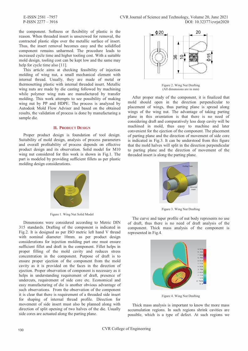
E-ISSN 2581 –7957 CVR Journal of Science and Technology, Volume 20, June 2021 P-ISSN 2277 – 3916 DOI: 10.32377/cvrjst2020
CVR College of Engineering
the component. Softness or flexibility of plastic is the reason. When threaded insert is unscrewed for removal, the contracted plastic slips over the metallic surface of insert. Thus, the insert removal becomes easy and the solidified component remains unharmed. The procedure leads to increased cycle time and higher tooling cost. With a suitable mold design, tooling cost can be kept low and the same may help for cycle time also [11].
This article aims at checking feasibility of injection molding of wing nut, a small mechanical element with internal thread. Usually, they are made of metal or thermosetting plastic with internal threaded insert. Metallic wing nuts are made by die casting followed by machining while polymer wing nuts are manufactured by transfer molding. This work attempts to see possibility of making wing nut by PP and HDPE. The process is analyzed by Autodesk Mold Flow Adviser and based on the obtained results, the validation of process is done by manufacturing a sample die.
II. PRODUCT DESIGN
Proper product design is foundation of tool design. Suitability of mold design, analysis of process parameters and overall profitability of process depends on effective product design and its observation. Solid model for M10 wing nut considered for this work is shown in Fig.1. The part is modeled by providing sufficient fillets as per plastic molding design considerations.
Figure 1. Wing Nut Solid Model
Dimensions were considered according to Metric DIN 315 standards. Drafting of the component is indicated in Fig.2. It is designed as per ISO metric left hand V thread with nominal diameter 10mm. as per product design considerations for injection molding part one must ensure sufficient fillet and draft in the component. Fillet helps in proper filling of the mold cavity and reduces stress concentration in the component. Purpose of draft is to ensure proper ejection of the component from the mold cavity as it is provided on the faces in the direction of ejection. Proper observation of component is necessary as it helps in understanding requirement of draft, presence of undercuts, requirement of side core etc. Economical and easy manufacturing of die is another obvious advantage of such observations. From the observation of the component it is clear that there is requirement of a threaded side insert for shaping of internal thread profile. Direction for movement of side insert must also be planned along with direction of split opening of two halves of the die. Usually side cores are actuated along the parting plane.
Figure 2. Wing Nut Drafting (All dimensions are in mm)
After proper study of the component, it is finalized that mold should open in the direction perpendicular to placement of wings, thus parting plane is spread along wings of the wing nut. The advantage of taking parting plane in this orientation is that there is no need of considering draft and comparatively less deep cavity will be machined in mold, thus easy to machine and later convenient for the ejection of the component. The placement of parting plane and the direction of movement of side core is indicated in Fig.3. It can be understood from this figure that the mold halves will split in the direction perpendicular to parting plane and the direction of movement of the threaded insert is along the parting plane.
Figure 3. Wing Nut Drafting
The curve and taper profile of nut body represents no use of draft, thus there is no need of draft analysis of the component. Thick mass analysis of the component is represented in Fig.4.
Figure 4. Wing Nut Drafting
Thick mass analysis is important to know the more mass accumulation regions. In such regions shrink cavities are possible, which is a type of defect. At such regions we

E-ISSN 2581 –7957 CVR Journal of Science and Technology, Volume 20, June 2021 P-ISSN 2277 – 3916 DOI: 10.32377/cvrjst2020
CVR College of Engineering
should remove mass by making weight reduction pockets. But for wing nut such remedies are not possible considering strength as criteria. But the situation is not very critical as the region is tapered and in a very shallow region thick mass accumulation is there. Additionally, by increasing holding pressure also, shrink cavities can be avoided.
III. PROCESS SIMULATION
Process simulation helps us to know proper gate position with respect to a component cavity, expected positions of vents, fill time, flow pattern, probable defects etc.
A. Material Selection The materials selected for this work is PP and HDPE.
Both are frequently available and widely used thermo plastics. PP is tough as well as flexible material while HDPE has superior mechanical properties. Their relative properties are enlisted in Table I.
TABLE I. MATERIAL SPECIFICATION
Material Properties PP HDPE Density 946 kg/m³ 970 kg/m³ Softening Point 150 °C 125 °C Formula (C3H6)n (C2H4)n Shrinkage 1-2.5% 1.5-3% Tensile Strength 21-37 N/mm² 19-39 N/mm² Injection Temperature 260 °C 240 °C Heat Deflection Temperature 120 °C 90 °C Mold Temperature 60°C 30°C
B. Process Parameter Selection Process parameters are selected from an injection
molding machine specification. The motive behind this was validation of result obtained from simulation with the trial results of the component. The specification of the considered injection molding machine is mentioned in Table II.
TABLE II. MACHINE SPECIFICATION
(TEXPLASST 1HD, MP LAB, CVRCE HYDERABAD)
Shot Capacity 2 – 45 gms / shot Plunger Diameter 25 mm Stroke Length 450mm Clamping Capacity 6.0 Tons Injection Pressure 80 kg/cm2 Heating Capacity 1.5 kw Total Installed Power 3.7 kw Total Shut Height 100 - 450mm
C. Simulation Results Based on the parameters discussed earlier, the flow
analysis was run using Autodesk Mold Flow Adviser. The results were satisfactory and helpful for die design corresponding to the component. Fig. 5 represents die cavity filling stages in clockwise direction from top left corner. The preferred gating position and flow of material around internal helical thread profile can be observed in the figure. Input parameters are separately entered to run the simulation for PP and HDPE materials. The flow analysis results were further compared.
Figure 5. Plastic Flow in Mold Cavity
Confidence of fill and quality prediction results was compared and the same is represented in Fig. 6. With both the materials probability of filling the die is high but quality prediction is not very high. It is medium in thread region for HDPE but for PP quality prediction is average for entire component. This result indicates that HDPE is more suitable for making wing nuts as quality prediction reflects mechanical properties and appearance of a component.
Figure 6. Confidence of Fill and Quality Prediction for PP( Top) and HDPE (Bottom)
The fill time estimated by the flow analysis indicates filling of cavity in 0.1 second with PP and 0.21 second for HDPE. This is quite possible as material flow in flow path is not considered. Additionally, shot volume is 2.32 cm3, total part weight is 1.71g for PP and 1.76g for HDPE. Fill time result is shown in Fig. 7.
Figure 7. Fill Time
E-ISSN 2581 –7957 CVR Journal of Science and Technology, Volume 20, June 2021 P-ISSN 2277 – 3916 DOI: 10.32377/cvrjst2020
CVR College of Engineering
The temperature variance result is represented in Fig. 8. This result helps us to identify areas with variable temperature so that cooling provision can be arranged accordingly. Maximum temperature is observed at thread region which can be further dissipated by threaded insert.
Figure 8. Temperature Variance
Temperature of flow front is indicated in Fig. 9. In case of both the materials the result is quite in agreement with assumption that the flow front should remain at high temperature so that complete filling of cavity can be ensured. Additionally, gate should solidify first so that directional solidification can be ensured and any back flow of material can be avoided. This also can be visualized in Fig. 9. This result is according to molding temperature of PP, 260°C and HDPE, 240°C.
Figure 9. Temperature at Flow Front
It is important to know the time to reach ejection temperature. This is measured from the starting time of filling the mold cavity and helps to estimate cycle time of the injection molding process. Fig. 10 represents this time for both the material and the software estimates the cycle time in case of PP and HDPE as 30.04 second and 30.80 second respectively.
Figure 10. Time to Reach Ejection Temperature
Weld line indicates angle of overlap of material flow fronts. They are unavoidable if flow fronts splits while filling a cavity. In case of this mold cavity around the internal thread profile, material flow is diverging. This can
be visualized from Fig. 5. Acute values of weld lines are acceptable and proper merger of flow fronts must be ensured by changing process parameters. Otherwise structural deficiency and surface imperfections are possible. To avoid weld lines, changing gate location, applying squeeze pressure, increasing melt temperature etc. can be attempted. Though there are smaller values of weld line angle for the component, we will apply squeeze pressure to overcome them as we are going to implement that for tackling shrink cavities. The weld line result with reference to both the materials in this work is shown in Fig. 11.
Figure 11. Weld Lines
The mold flow result indicates shrink cavities or sink marks also, as they were expected from thick mass analysis and shown in Fig. 4. Approximately same amount of sink mark was observed in thick mass region for both the materials, as shown in Fig. 12.
Figure 12. Sink Marks
The software indicated details of sink mark corresponding to both the materials which is shown in Table III. The amount of sink mark is minute but it can be avoidedby making mass reduction pockets in that portion which is not advisable as per design and strength criteria of wing nut. We opt to apply squeeze pressure or packing pressure to overcome shrinkage cavities. There were no indications of warpage or any other type of defects.
TABLE III. SINK MARK DETAILS
Material Properties PP HDPE Maximum Sink Depth 0.25mm 0.25mm Average Sink Mark Depth 0.04mm 0.04mm Model Prone to Sink Mark 0.62% 0.60%
IV. DIE TRIAL
From the satisfactory flow analysis results, a die was modeled. This die was prepared only for trial purpose and is unlike the actual injection molding die which is prepared for industrial purpose. An injection molding die prepared for actual manufacturing process consists of proper provision of

E-ISSN 2581 –7957 CVR Journal of Science and Technology, Volume 20, June 2021 P-ISSN 2277 – 3916 DOI: 10.32377/cvrjst2020
CVR College of Engineering
handling mismatch, mold cooling and ejection of the component. To achieve mass production, base on size of the component they are usually of multiple cavities.
A. Mold Design The modeled die consisted single cavity and flow path. It
has taper to take care of mismatch. No additional provision of mold cooling was given and ejection was also planned manually. The design was done considering ease of manufacturing. Based on overall volume of cavity runner length and diameter was taken from tool design parameter handbook from CITD. The assembly of modeled die is shown in Fig. 13 along with part and insert in its position. Runner of 4mm diameter and 30mm length can be observed, while gate diameter is 2mm and it is 3mm long. Taper on edges of core and cavity can be observed on the edges to avoid mismatch. Mold cavity and flow path are equally split in core and cavity.
Figure 13. Model Mold
B. Die Trial The model die was manufactured by EN 19 material.
Overall shape was then turned at top and bottom. It was milled resting and aligning with feed system of injection molding machine. The part profile was cut by CNC milling with ball nose cutter. The trial was taken on injection molding machine at CVRCE as specified in Table II. Near to fifty shots were taken with PP and HDPE materials. The shot of first trial is shown in Fig. 14.
Figure 14. The Die Trial
Similarly, in the simulation results, there were no defects found on the component. There were no weld lines on the surface and no shrinking mark over the bottom portion of the molded wing nut. Additional holding pressure was applied in each shot to overcome shrinkage and the same can be visualized from Fig. 15.
Figure 15. Molded Wing Nuts
V. CONCLUSIONS
With recent advances in materials and manufacturing technology it is ultimately possible to process any material by any manufacturing process. One must always see economy and feasibility of the process. Wing nuts are usually made of metal and irrespective of their primary shaping process they must come across machining operation for obtaining internal thread profile. Multiple operations lead to high cost of manufacturing a component. In terms of economic and manufacturing feasibility it is advisable to make wing nuts by injection molding process. But based on strength criteria and related to end use of the product, application of wing nut made of polymer is limited to optimum strength, light weight and corrosion resistant applications. Scope of this work is limited to evaluating feasibility of making wing nuts by injection molding process using different polymers. Optimization of process parameters and molding wing nuts by a type of polymer with comparable properties of a metal can be further scope of research work.
REFERENCES [1] R.Sánchez, A.Martinez, D.Mercado, A.CarbonelJ.Aisa,
“Rapid heating injection moulding: An experimental surface temperature study”, Polymer Testing, Volume 93, 2021, 106928
[2] Neeraj Kumar Jha, Bhavya Sri Tadiparthi, “Design and Analysis of the Sleeve Ejection System in Injection Molding Die for Trolley Wheel”, CVRJST, Vol. - 17, pp. 132-137, 2019.
[3] Giovanni Lucchetta, Davide Masato, Marco Sorgato, “Optimization of mold thermal control for minimum energy consumption in injection molding of polypropylene parts”, Journal of Cleaner Production,Vol.- 182, 2018, pp. 217-226.
[4] N. Sateesh, S. Devakar Reddy, G. Praveen Kumar, Ram Subbiah,” Optimization of injection moulding process in manufacturing the flip cover of water meter”, Materials Today: Proceedings 26, 2020, pp. 240-246.
[5] Abdulmecit Güldaş, Onuralp Uluer & Ahmet Özdemir, “The Numerical Analysis of a Mold Cavity Filling Using the Finite Control Volume Method and Comparison to the Experimental Results”, Polymer-Plastics Technology and Engineering, 48:4, 2009 , pp. 389-396.
[6] Marton Huszar, Fawzi Belblidia, Helen M.Davies, Cris Arnold, David Bould, Johann Sien, “Sustainable injection moulding: The impact of materials selection and gate location on part warpage and injection pressure”, Sustainable Materials and Technologies Vol.- 5, 2015, pp. 1-8.

E-ISSN 2581 –7957 CVR Journal of Science and Technology, Volume 20, June 2021 P-ISSN 2277 – 3916 DOI: 10.32377/cvrjst2020
CVR College of Engineering
[7] Jiseon Hong, Sun Kyoung Kim, Young-Hak Cho, “Flow and solidification of semi-crystalline polymer during micro-injection molding”, International Journal of Heat and Mass Transfer Vol.- 153, June 2020, 119576.
[8] Babur Ozcelik , Alper Ozbay, Erhan Demirbas, “Influence of injection parameters and mold materials on mechanical properties of ABS in plastic injection molding”, International Communications in Heat and Mass Transfer, Vol.- 37, Issue 9, 2010, pp. 1359-1365.
[9] E.Farotti, M.Natalini, “Injection molding. Influence of process parameters on mechanical properties of polypropylene polymer. A first study”, Procedia Structural Integrity, Vol.- 8, 2018,pp. 256-264.
[10] Neeraj Kumar Jha, P V Ramana, “Design Methodology and Analysis of Double Cavity Metal-Plastic-Insert Injection Molding Die for Push Board Pin”. CVRJST, Vol. - 14, pp. 91-96, 2018.
[11] Simion Haragas, Ovidiu Buiga, Ovidiu Buiga, Claudiu Popa, Florina Maria , ȘerdeanFlorina, Maria Șerdean,” Demolding Moment Calculation for Injected Parts with Internal Saw Thread”, MATERIALE PLASTICE, 2016, 53(3):378-381

E-ISSN 2581 – 7957 CVR Journal of Science and Technology, Volume 20, June 2021 P-ISSN 2277 – 3916 DOI: 10.32377/cvrjst2021
CVR College of Engineering
Simulation Analysis of Additive Manufacturing of Impeller
hru Technological University/Mechanical Engg. Hyderabad, India Email: [email protected]
Abstract: An Impeller is the rotating component of a pump; it transfers the energy from the motor to the fluid and accelerates the fluid to build up pressure. Impellers are manufactured using Additive Manufacturing (AM) technology. It is a technology that produces three-dimensional parts layer by layer from a variety of materials such as plastics, polymers and metals. The impeller is usually made up of Stainless Steel 316L, Inconel 718. AM technique used to manufacture impeller is Direct Metal Laser Sintering (DMLS). The main objective of this paper is to conduct simulation analysis of additive manufacturing of an impeller by varying process-parameters such as Power, Wall-thickness and Angle and recommend a suitable material with minimum von-misses stress, minimum displacement and minimum of maximum temperature using Amphyon software. Simulation analysis is performed on two different materials i.e., Stainless Steel 316L and Inconel 718 by varying process parameters such as Power at 200 to 400W, Wall thickness at 0.5 to 0.8mm and Angle at 00 to 60. Amphyon is a modular pre-processing and simulation software for Laser Beam Melting (LBM) processes. The simulation results were analyzed and optimization for Stainless-Steel 316L material impeller was done using one of the MADM methods i.e., Technique for Order of Preference by Similarity to Ideal Solution (TOPSIS) method. Later, the results of the two different materials (i.e., Stainless Steel 316L and Inconel 718) were compared. Stainless Steel 316L was found to have minimum von-misses stress, minimum displacement and minimum of maximum temperature at 200W power, 0.5mm wall-thickness and 00 angle.
Index Terms: Impeller, Additive Manufacturing, Direct Metal Laser Sintering (DMLS), Amphyon, MADM, TOPSIS.
I. INTRODUCTION
Impeller is a rotating element of a centrifugal pump which helps to accelerate the fluid outward from the center of the rotation, thereby transferring energy required from the motor that drives the pump to the motor driven by the fluid [1,2]. Various manufacturing techniques are used to build an impeller such as traditional manufacturing (i.e., casting), Additive Manufacturing (i.e., powder bed fusion method) and Hybrid Manufacturing which combines both traditional and additive manufacturing methods that makes it more effective [3]. The Additive manufacturing (AM) or 3D printing techniques have gained immense popularity for its ability to make complex objects such as impeller [4]. It also introduces the possibility for new products, largely due to greater design liberty. AM is a preferred process as it adds material layer by layer thereby reducing the wastage of material when compared to traditional manufacturing which
removes the material. AM has a wide range of applications with different variety of materials such as plastics, polymers and metals [5]. The impeller is usually made of Stainless Steel 316L and Inconel 718 as both these materials have high corrosion resistance. Both these materials are anisotropic in nature i.e., they show different behaviour
observed that the maximum anisotropic deformation is found at 450 for both the materials [6,7]. The AM method used to manufacture metal products is Laser Power Bed Fusion method. One of the LPBF technique used to manufacture impeller is Direct Metal Laser Sintering (DMLS) [8,9,10,11,12] as it has a wide range of materials such as Stainless steel 316l, Inconel718, Ti6Al4V, Stainless steel 17-PH. The principle behind this method is the application of thin layers of metal powder using a re-coater blade. The metal powder is sintered by a collimated laser beam, which fuses the particles of the metal together to create a solid material. The main objective of this paper is to conduct a simulation analysis of additive manufacturing of an impeller and to recommend a suitable material for manufacturing with minimum Von-misses stress, minimum Displacement and minimum of maximum Temperature by varying various process-parameters such as Power (200W to 400W), Wall-thickness (0.5mm to 0.8mm) and Angle (00 to 60) using Amphyon software. Amphyon is a modular pre-processing and simulation software for Laser Beam Melting (LBM) processes. The values of power, wall-thickness and angles are considered based on the following recommendations. The wall thickness above 0.5mm is considered to avoid warpage in the components [13,14]. The power impacts the micro-structure of the material thus two different laser powers are being considered [15] and according to the Amphyon software simulation assessment these orientations angles (i.e., 00 to 60) with respect to build plate was recommended for the material and build conditions mentioned earlier. Based on the above build parameters EOSINT M280 machine is considered for simulation. The simulation values were recorded. The simulation results of stainless steel were analyzed and optimization was performed using one of the Multi Attribute Decision Making (MADM). The technique used to perform optimization was Technique for Order of Preference by Similarity to Ideal Solution (TOPSIS) [16].
along the different directions of the materials. It has been
1 G Scholar, Jawaharlal Nehru Technological University/Mechanical Engg. Hyderabad, India
2Professor, Jawaharlal NeEmail: [email protected]
K. Varsha1 and Dr. M. Indira Rani2

E-ISSN 2581 – 7957 CVR Journal of Science and Technology, Volume 20, June 2021 P-ISSN 2277 – 3916 DOI: 10.32377/cvrjst2021
CVR College of Engineering
B. Machine Specifications The machine used is EOSINT M 280. The machine
comprises a process chamber with recoating system, elevating system and platform heating module, an optical system with laser, a process gas management system, a process computer with process control software, and a set of standard accessories. The machine components are integrated into a robust machine frame. During operation the process chamber is secured by interlock. The specifications are shown in the Table V.
TABLE III. COMPOSITION OF INCONEL 718
Element Mass (%)
Nickel 50-55
Chromium 17-21
Niobium and tantalum 4.75-5.5
Molybdenum 2.80-3.30
Titanium 0.65-1.15
Cobalt ≤ 1.00
Aluminum 0.20 -0.80
Manganese ≤ 0.35
Silicon ≤ 0.35
Copper ≤ 0.30
Carbon 0.02 – 0.05
Nitrogen ≤ 0.03
Oxygen ≤ 0.03
Phosphorous ≤ 0.015
Sulphur ≤ 0.015
Calcium ≤ 0.01
Magnesium ≤ 0.01
Selenium ≤ 0.005
Boron ≤ 0.005
Iron Balance
TABLE IV. MECHANICAL PROPERTIES OF INCONEL 718
Property Value
Ultimate tensile Strength 676 MPa
Yield Stress 541 MPa
Young’s modulus 178 GPa
Poisson’s ratio 0.3
II. MATERIALS AND MACHINE SPECIFICATION
A. Materials The materials used to manufacture impeller are Stainless
Steel 316L and Inconel 718 as they have high corrosion resistance.
Stainless Steel: The composition and mechanical properties are shown in Table I and Table II.
Material properties: 1. High hardness and toughness.2. High corrosion resistance.3. High machine-ability.4. Can be highly polished.
TABLE I. PROPERTIES OF STAINLESS STEEL 316L
Property Value
Ultimate tensile Strength 1467 MPa
Yield Stress 1150 MPa
Young’s modulus 205 GPa
Poisson’s ratio 0.3
TABLE II. COMPOSITION OF STAINLESS STEEL 316L
Element Concentration [Wt.%] Acc. ASTM A276
Carbon ≤ 0.03
Manganese ≤ 2
Silicon ≤ 1
Nitrogen ≤ 0.1
Phosphorous ≤ 0.045
Sulphur ≤ 0.015
Molybdenum 2-3
Chromium 16-18
Nickel 10-14
Iron Balance
Manganese ≤ 0.03
Inconel 718: The composition and mechanical properties are shown in Table III and Table IV.
Material properties: 1. Retains strength up to 650 °C.2. High creep resistance.3. High corrosion resistance.4. Solidification properties suit additive manufacture.

E-ISSN 2581 – 7957 CVR Journal of Science and Technology, Volume 20, June 2021 P-ISSN 2277 – 3916 DOI: 10.32377/cvrjst2021
CVR College of Engineering
C. Amphyon Software Amphyon is a modular pre-processing and simulation
software for laser beam melting (LBM) processes. The Amphyon modules can be used in pre-processing chains from CAD to build job by replacing or improving several stages. Driven by industrial needs and requirements in LBM processes, an innovative new pre-process chain was derived. Three main stages on the way to a stable, efficient and reliable process were identified.
Figure 1. The ASAP Principle
The mechanical simulation model in Amphyon uses an approach called Inherent Strain approach. The basic principle of the inherent strain approach for additive manufacturing is that if no external loads are applied, the inherent strains is defined as the sum of plastic and thermal strains which completely defines the stress state and the deformation within a given domain. The inherent strain approach for additive manufacturing is also called Mechanical Layer Equivalent (MLE) Method.
The thermal simulation model in Amphyon uses an approach of Global Thermal Analysis. The build rate and the amount of time for cooling down between consecutive
layers is one of the most important influencing factors for the macro scale thermal simulation of the process. If the cool down time between layers is increases by a factor of two, the macro scale thermal field is reduced by approximately the same factor if non-linear influences such as radiation, convection, absorption etc. are neglected.
D. Methodology The steps involved in the simulation analysis is shown in
the Figure 2. Twelve different simulation analysis are done for each material by varying the power (200W, 400W), wall-thickness (0.5mm, 0.8mm) and angle (00, 20, 50) respectively. The impellers with different angles with respect to build plate and their supports are shown in the Figure 3.
Figure 2. Flow-chart of steps involved in Simulation process
(a) (b) (c)
Figure 3. Supports generated to impeller build at different angles w.r.t build plate. (a) 00 angle (b) 20 angle (c) 50 angle
E. Boundary conditions Mechanical simulations: � Material is anisotropic, max deformation at 450. � Heat treatment: After the release of the base, stresses to
zero Thermal simulations: � Preheating of the build area at 500 C. � Energy transferred into the part. � Evaporation the material � Convection on the outside surface of Heat affected
zone.
TABLE V. EOSINT M 280 MACHINE TECHNICAL DATA
Effective building volume 250mm×250mm×215mm
Building speed (material- dependent)
2-20 mm3/s (0.0001 – 0.001 in3/sec)
Laser Power 200 W or 400 W
Laser Type Yb-fiber laser
Scan Speed Up to 7.0 m/s
Power Supply 32A
Layer Thickness 20 – 60 μm
Power Consumption Max 8.5kW/ typical 3.2 kW
Precision Optics F-theta- lens, high- speed scanner
Variable focus diameter 100 – 500 μm
Nitrogen generator Standard
Dimensions:
System 2000mm×1050mm×1940mm Recommended installation
space Approx. 3.5m×3.6m×2.5m
Weight Approx. 1130kg

E-ISSN 2581 – 7957 CVR Journal of Science and Technology, Volume 20, June 2021 P-ISSN 2277 – 3916 DOI: 10.32377/cvrjst2021
CVR College of Engineering
III. RESULTS
The results of the simulation are shown in the Table VI and Table VII. The tables consist of the values of von-misses stress, displacement and maximum temperature of Stainless steel 316L and Inconel 718.
Optimization: Table VIII shows minimum stress and displacement at 200W, 00 and 0.5mm wall-thickness and minimum value of maximum temperature occurs at 200W, 50 and 0.5mm wall-thickness. To resolve this ambiguity, one of the MADM techniques i.e., Technique for Order of Preference by Similarity to Ideal Solution (TOPSIS) is used. The process is carried out as follows: Step 1: Create an evaluation matrix
Step 2: Obtain normalized decision matrix Xij*=
TABLE V II. DECISION TABLE
Beneficial
Power (W)
Wall Thickness
(mm) Angle Von-Misses
(MPa)
Max Temperature
(0C)
Displacement (mm)
200 0.5 0 0.071665 58.1 0.189
200 0.5 2 0.2580 57.17 0.241
200 0.5 5 0.156 47.4 0.343
200 0.8 0 0.114 59.40 0.266
200 0.8 2 0.209 59.75 0.323
200 0.8 5 0.546 53 0.411
400 0.5 0 0.0729 69.206 0.1905
400 0.5 2 0.4089 69.59 0.242
400 0.5 5 0.2058 75.71 0.3427
400 0.8 0 0.4912 69.05 0.269
400 0.8 2 0.4589 69.226 0.322
400 0.8 5 0.3039 85.644 0.412
TABLE VII. VALUES OF STAINLESS STEEL 316L
Power (W)
Wall Thickness
(mm) Angle
Von-Misses (MPa)
Max Temperature
(C)
Displacement (mm)
200 0.5 0 0.118 59.504 0.245
200 0.5 2 0.7448 59.74 0.288
200 0.5 5 0.303 62.328 0.370
200 0.8 0 0.1669 59.560 0.300
200 0.8 2 0.190136 59.649 0.337
200 0.8 5 0.600 67.9 0.439
400 0.5 0 0.1539 69.23 0.246
400 0.5 2 0.5120 69.97 0.285
400 0.5 5 0.555 75.15 0.369
400 0.8 0 0.4912 69.05 0.269
400 0.8 2 0.4589 69.226 0.322
400 0.8 5 0.3039 85.644 0.412
TABLE VI. VALUES OF INCONEL 718
Power (W)
Wall Thickness
(mm) Angle Von-Misses
(MPA)
Max Temperature
(C)
Displacement (mm)
200 0.5 0 0.118 59.504 0.245
200 0.5 2 0.7448 59.74 0.288
200 0.5 5 0.303 62.328 0.370
200 0.8 0 0.1669 59.560 0.300
200 0.8 2 0.190136 59.649 0.337
200 0.8 5 0.600 67.9 0.439
400 0.5 0 0.1539 69.23 0.246
400 0.5 2 0.5120 69.97 0.285
400 0.5 5 0.555 75.15 0.369
400 0.8 0 0.1948 69.468 0.300
400 0.8 2 0.3127 69.656 0.335
400 0.8 5 0.53029 86.12 0.438 TABLE IX.
VALUES OF Xi2 AND
Xi2 1.20991799 51057.4803 1.11354354
SQRT(∑Xi2) 1.09996272 225.959024 1.05524572
TABLE X. NORMALIZED TABLE
Power (W)
Wall Thickness
(mm) Angle Von-Misses
(MPa)
Max Temperatur
e (0C)
Displacement (mm)
200 0.5 0 0.0051358 3375.61 0.035721
200 0.5 2 0.066564 3268.4089 0.058081
200 0.5 5 0.024336 2246.76 0.117649
200 0.8 0 0.012996 3528.36 0.070756
200 0.8 2 0.043681 3570.0625 0.104329
200 0.8 5 0.298116 2809 0.168921
400 0.5 0 0.0053144 4789.4704 0.03629025
400 0.5 2 0.1671992 4842.7681 0.058564
400 0.5 5 0.0423536 5732.0041 0.11744329
400 0.8 0 0.2412774 4767.9025 0.072361
400 0.8 2 0.2105892 4792.2390 0.103684
400 0.8 5 0.0923552 7334.8947 0.169744

E-ISSN 2581 – 7957 CVR Journal of Science and Technology, Volume 20, June 2021 P-ISSN 2277 – 3916 DOI: 10.32377/cvrjst2021
CVR College of Engineering
Step 4: Determine the worst and the best alternative.
Step 5: Calculate Separation Measures
Step 6: Calculate relative closeness to positive ideal solution Pi = and rank them.
From the above table we can conclude that the best optimal result is found at 200W, 00 angle and 0.5mm wall-thickness.
TABLE XV. RANK TABLE
Pi Rank
0.180254 0.913307 1
0.170828 0.646331 5
0.186891 0.708341 4
0.176151 0.815938 3
0.174034 0.645329 6
0.207386 0.229889 12
0.192749 0.834749 2
0.179794 0.397151 8
0.181533 0.58525 7
0.186756 0.286476 10
0.173823 0.261262 11
0.186985 0.391972 9
TABLE XIV. NORMALIZED WEIGHT TABLE
S. No. S+ S-
1 0.015627 0.164627
2 0.060417 0.110412
3 0.054509 0.132383
4 0.032423 0.143728
5 0.061725 0.112309
6 0.15971 0.047676
7 0.031852 0.160897
8 0.108388 0.071405
9 0.075291 0.106242
10 0.133255 0.053501
11 0.128409 0.045413
12 0.113692 0.073293
TABLE XIII. VALUES OF V+ and V-
V+ 0.02169569 0.06922494 0.05910472 V+
V- 0.16529469 0.12507808 0.12884203 V-
TABLE XII. NORMALIZED WEIGHT TABLE
S. No. Von-Misses (MPa)
Max Temperature (0C)
Displacement (mm)
1 0.02169569 0.08485167 0.05910472
2 0.07810628 0.08349346 0.07536633
3 0.04722705 0.06922494 0.10726412
4 0.03451208 0.08675024 0.08318442
5 0.06327214 0.0872614 0.10100965
6 0.16529469 0.07740341 0.12852931
7 0.02206957 0.10107133 0.0595738
8 0.12378938 0.10163214 0.07567906
9 0.06230338 0.11057005 0.1071703
10 0.14870468 0.10084351 0.08412259
11 0.13892625 0.10110054 0.10069693
12 0.09200194 0.12507808 0.12884203
TABLE XI. CALCULATION OF WEIGHTS
S. No. Von-Misses (MPa)
Max Temperature
(0C)
Displacement (mm)
Weights 0.33 0.33 0.33
1 0.06515221 0.25712627 0.1791052
2 0.2345534 0.25301048 0.22838283
3 0.14182299 0.20977255 0.32504278
4 0.10363988 0.26287952 0.25207399
5 0.19000644 0.26442847 0.30608984
6 0.49638046 0.2345558 0.38948274
7 0.06627497 0.30627677 0.18052667
8 0.37173987 0.30797619 0.22933047
9 0.18709725 0.33506075 0.32475848
10 0.44656059 0.30558638 0.25491693
11 0.41719596 0.30636528 0.3051422
12 0.27628209 0.37902447 0.39043039
Step 3: Calculate the weighted normalized decision matrix
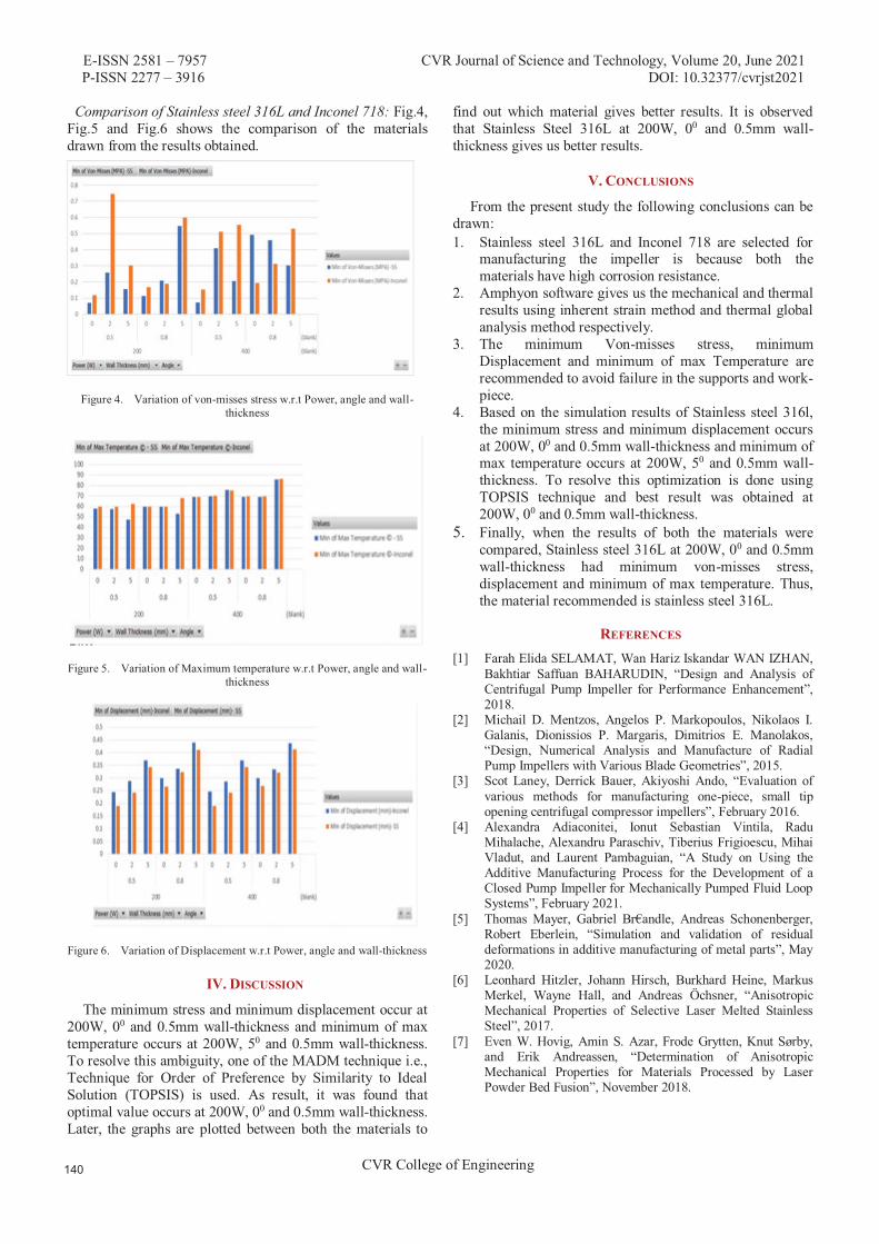
E-ISSN 2581 – 7957 CVR Journal of Science and Technology, Volume 20, June 2021 P-ISSN 2277 – 3916 DOI: 10.32377/cvrjst2021
CVR College of Engineering
Comparison of Stainless steel 316L and Inconel 718: Fig.4, Fig.5 and Fig.6 shows the comparison of the materials drawn from the results obtained.
Figure 4. Variation of von-misses stress w.r.t Power, angle and wall-thickness
Figure 5. Variation of Maximum temperature w.r.t Power, angle and wall-thickness
Figure 6. Variation of Displacement w.r.t Power, angle and wall-thickness
IV. DISCUSSION
The minimum stress and minimum displacement occur at 200W, 00 and 0.5mm wall-thickness and minimum of max temperature occurs at 200W, 50 and 0.5mm wall-thickness. To resolve this ambiguity, one of the MADM technique i.e., Technique for Order of Preference by Similarity to Ideal Solution (TOPSIS) is used. As result, it was found that optimal value occurs at 200W, 00 and 0.5mm wall-thickness. Later, the graphs are plotted between both the materials to
find out which material gives better results. It is observed that Stainless Steel 316L at 200W, 00 and 0.5mm wall-thickness gives us better results.
V. CONCLUSIONS
From the present study the following conclusions can be drawn: 1. Stainless steel 316L and Inconel 718 are selected for
manufacturing the impeller is because both the materials have high corrosion resistance.
2. Amphyon software gives us the mechanical and thermal results using inherent strain method and thermal global analysis method respectively.
3. The minimum Von-misses stress, minimum Displacement and minimum of max Temperature are recommended to avoid failure in the supports and work-piece.
4. Based on the simulation results of Stainless steel 316l, the minimum stress and minimum displacement occurs at 200W, 00 and 0.5mm wall-thickness and minimum of max temperature occurs at 200W, 50 and 0.5mm wall-thickness. To resolve this optimization is done using TOPSIS technique and best result was obtained at 200W, 00 and 0.5mm wall-thickness.
5. Finally, when the results of both the materials were compared, Stainless steel 316L at 200W, 00 and 0.5mm wall-thickness had minimum von-misses stress, displacement and minimum of max temperature. Thus, the material recommended is stainless steel 316L.
REFERENCES [1] Farah Elida SELAMAT, Wan Hariz Iskandar WAN IZHAN,
Bakhtiar Saffuan BAHARUDIN, “Design and Analysis of Centrifugal Pump Impeller for Performance Enhancement”, 2018.
[2] Michail D. Mentzos, Angelos P. Markopoulos, Nikolaos I. Galanis, Dionissios P. Margaris, Dimitrios E. Manolakos, “Design, Numerical Analysis and Manufacture of Radial Pump Impellers with Various Blade Geometries”, 2015.
[3] Scot Laney, Derrick Bauer, Akiyoshi Ando, “Evaluation of various methods for manufacturing one-piece, small tip opening centrifugal compressor impellers”, February 2016.
[4] Alexandra Adiaconitei, Ionut Sebastian Vintila, Radu Mihalache, Alexandru Paraschiv, Tiberius Frigioescu, Mihai Vladut, and Laurent Pambaguian, “A Study on Using the Additive Manufacturing Process for the Development of a Closed Pump Impeller for Mechanically Pumped Fluid Loop Systems”, February 2021.
[5] Thomas Mayer, Gabriel Br€andle, Andreas Schonenberger, Robert Eberlein, “Simulation and validation of residual deformations in additive manufacturing of metal parts”, May 2020.
[6] Leonhard Hitzler, Johann Hirsch, Burkhard Heine, Markus Merkel, Wayne Hall, and Andreas Öchsner, “Anisotropic Mechanical Properties of Selective Laser Melted Stainless Steel”, 2017.
[7] Even W. Hovig, Amin S. Azar, Frode Grytten, Knut Sørby, and Erik Andreassen, “Determination of Anisotropic Mechanical Properties for Materials Processed by Laser Powder Bed Fusion”, November 2018.

E-ISSN 2581 – 7957 CVR Journal of Science and Technology, Volume 20, June 2021 P-ISSN 2277 – 3916 DOI: 10.32377/cvrjst2021
CVR College of Engineering
[8] Peiying Bian, Xiaodong Shao, and Jingli Du, “Finite Element Analysis of Thermal Stress and Thermal Deformation in Typical Part during SLM", 28 May 2019.
[9] Kai Zhan, Tingting Liu, Wenhe Liao, Changdong Zhang, Yi Zheng, Huang Shao, “Simulation of The Thermal Behaviour and Analysis of Solidification Process During Selective Laser Melting of Alumina”, 2018.
[10] C. Y. Yap, C. K. Chua, Z. L. Dong, Z. H. Liu, D. Q. Zhang, L. E. Loh, and S. L. Sing, “Review of selective laser melting: Materials and applications”, 2015.
[11] Röttger, J. Boes, W. Theisen, M. Thiele, C. Esen, A. Edelmann, and R. Hellmann, “Microstructure and mechanical properties of 316L austenitic stainless steel processed by different SLM devices”, 30 September 2019.
[12] Milan Daňa, Ivana Zetková, and Josef Mach, “Mechanical Properties of Inconel Alloy 718 Produced by 3D Printing using DMLS”, September 2018.
[13] Johanna timhagen daniel nalumm, “Study of wall thickness and its impact on microstructure on 316L manufactured with Direct Metal Laser Sintering”, 2017.
[14] “Guidelines for Wall Thickness in Laser Sintering: Guidelines for Wall Thickness in Laser Sintering” | Additive Manufacturing [Accessed on February 2021].
[15] Hahn Choo, Kin-Ling Sham, John Bohling, Austin Ngo, Xianghui Xiao, Yang Renb , Philip J. Depond, Manyalibo J. Matthews, Elena Garlea, “Effect of laser power on defect, texture, and microstructure of a laser powder bed fusion processed 316L stainless steel”, 2018.
[16] Ali Jozaghi, Babak Alizadeh, Mohsen Hatami, Ian Flood, Mohammad Khorrami, Nastaran Khodaei, and Erfan Ghasemi Tousi, “A Comparative Study of the AHP and TOPSIS Techniques for Dam Site Selection Using GIS: A Case Study of Sistan and Baluchestan Province, Iran”, December 2018.
[17] Paul Swartz, “Evaluation of Tensile Properties for Selective Laser Melted 316l Stainless Steel and The Influence of Inherent Process Features on Static Performance”, June 2019.
[18] K. Kamarudin, M.S Wahab, A.A. Raus, Aqeel Ahmed, and S Shamsudin, “Benchmarking of Dimensional Accuracy and Surface Roughness for AlSi10Mg Part by Selective Laser Melting (SLM)”, 2017.
[19] Altaf Ahmed, Arfan Majeed, Zahid Atta, and Guozhu Jia, “Dimensional Quality and Distortion Analysis of Thin-Walled Alloy Parts of AlSi10Mg Manufactured by Selective Laser Melting”, 2019.
[20] Nils Keller, John Schlasche, Hongxiao Xu, and Vasily Ploshikhin, Simulation Aided Manufacturing Scanning Strategies for Low Distortion in Laser Beam Melting Processes”, 2016.
[21] Elham Mirkoohi, Hong-Chuong Tran, Yu-Lung Lo, You-Cheng Chang, Hung-Yu Lin, and Steven Y. Liang, “Analytical Modeling of Residual Stress in Laser Powder Bed Fusion Considering Part’s Boundary Condition”, April 2020.
[22] Tae-Jun Kim, Beom-Seon Jang, and Sung-Wook Kang, “Welding deformation analysis based on improved equivalent strain method considering the effect of temperature gradients”, 2015.
[23] Thoufeili Taufek, Yupiter HP Manurung, Stephan Lüder, Marcel Graf, and Farrahshaida Mohd Salleh, “Distortion Analysis of SLM Product of SS316L using Inherent Strain Method”, 2019.
[24] Suvi Santa-aho, Mika Kiviluoma, Tuomas Jokiaho, Tejas Gundgire, Mari Honkanen, Mari Lindgren, and Minnamari Vippola, “Additive Manufactured 316L Stainless-Steel Samples: Microstructure, Residual Stress and Corrosion Characteristics after Post-Processing”, January 2021.
[25] Santosh Kumar Parupelli, and Salil Desai, “A Comprehensive Review of Additive Manufacturing (3D Printing): Processes, Applications and Future Potential, 2019.
[26] “A Review on Direct Metal Laser Sintering: Process Features and Microstructure Modeling”, Available from: https://www.researchgate.net/publication/334504563_A_Review_on_Direct_Metal_Laser_Sintering_Process_Features_and_Microstructure_Modeling [accessed Feb 26 2021]
E-ISSN 2581 –7957 CVR Journal of Science and Technology, Volume 20, June 2021 P-ISSN 2277 – 3916 DOI: 10.32377/cvrjst2022
CVR College of Engineering
Effects of Fiber Orientation on Mechanical Properties and Analysis of Failures for Kevlar
Epoxy Reinforced Composites
E-mail: [email protected] 2Asst. Professor, CVR College of Engineering/Mechanical Engg. Department, Hyderabad, India.
E-mail: [email protected]
Abstract: This paper is an outcome of investigation made on Kevlar epoxy composites made by altering the fiber orientation. It is an important region to emphasize the effect of fiber angle in the composite that results in performance. In the present research the Kevlar fiber is made by 18 layers with different angular orientation from 0o to 90o. While preparing the composite the reinforcement is made by the addition of SiC and acetone to have the firm binding ability. In addition to that right from the first layer of the fiber to the 18th layer the angle is varied progressively from 0o to 90o. After the fabrication process the Kevlar composite is tested as a flat plate and a flat plate with a circular hole in it. The analysis has involved the maximum stress theory and Tsai-wu theory for the findings on fiber orientation against failure. The test results have yielded that the fiber orientation has the significant effect on the composite plate with a circular hole in it.
Index Terms: Kevlar epoxy composites, Mechanical characterization, Failure analysis
I. INTRODUCTION
Composites are a type of materials; possessing the properties that are to be tailored for meeting the higher level of anticipations including the aero space applications and outer space applications [1]. Researchers Mali et al [2] and Abd-Ali et. [3] had established the evidence by amending the fiber orientation with different angles in a type of composite laminate; hence, tracked down the different strengths that are to be accomplished. Hashimoto et al. [4] performed the research on tensile strength properties on the discontinuous and non uniform carbon fiber or polypropylene based composite with the disbursal of fiber direction. The exploration has proposed a ply-wise method to anticipate the discontinuous and non uniform fiber reinforced composite’s strength in tension and also the simple micro-mechanical investigation. The analysis has yielded the principle of combining is efficient & effective for the qualitative anticipation of mechanical strength and witnessed the accuracy hang on fiber direction distribution in the composites. Retnam et al. [5] have also studied the consequences of the fiber direction on mechanical properties such as strength of the hybrid glass / bamboo fiber based polymer composites. In that study, the mechanical possessions of composites are tested using the tensile test, impact test and flexural test before the repercussion was analyzed using the Scanning Electron Microscope (SEM).
The study divulges that the assimilation of composites escalate the mechanical properties next to improving the binding ability between the polyester resin and fiber. Due to its virtuosity and ruggedness, the Kevlar composite is one among the other composites that are chosen as advanced materials for the newfangled aircrafts. [6] In continuation with the engrossment, the researchers have started ushering studies in the domain of composite material. The cramming of composites have influenced the cut-out hole on the multilayered Kevlar/epoxy composite veneered plates has ushered by Talib et al. [7] for exploring the heterogeneity of acclimatization angles of the Kevlar fiber composite. The swatting was performed by the experimental ensuing by the simulation man oeuvre AUTODYN a part of ANSYS-12.1 software. With the outcomes, it was opined that the fiber angle and hole direction has influenced the Kevlar/epoxy composite material’s stiffness and strength. Gillespie Jr and Nilakantan. [8] also ushered a study on plain woven type Kevlar fabrics to find the reverberations of yarn sizing, fabric pre-tension and pullout rate. The investigation in this research exemplified the potential to the tactical tailoring of the yarn surface and yarn sizing characteristics to hone the ballistic whack performance of Kevlar fabric. Despite the enormous studies on the characteristics of the composite materials however there is yet a lack of studies that are related to the Kevlar/epoxy composites; thus, the etiquette of these characteristics are to be understood further. Hence, the motto of this research paper is to explore the reverberations of fiber orientation angle to conventionally woven Kevlar/Epoxy composites under the compression mode with the finite element analysis (FEA) software such as ANSYS.
Sapuan et al. [9] has made the research on kevlar epoxy reinforced composites with the fillers of coconut shell and also reported that the flexural and tensile strength of the Kevlar composites are increased with an improvement in the matter of the fillers of coconut shell. The composites evinced tensile stress in linear behavior associated with sharp fracture. Likewise, Thakur and Singha [10] divulged the mechanical traits of Phenol Formaldehyde matrix type reinforced composite with a fiber named Hibiscus Sabdariffa. It is babbled that particulate reinforcement fiber is more divulge than tiny fiber in tensile strength of composites. The strength in compression of fiber composite is also revamped than the base polymer. Xu et al. [11] explored the mechanical properties of Kevlar epoxy
1UG Scholar, CVR College of Engineering/Mechanical Engg. Department, Hyderabad, India. P. V. Sai Swaroop 1 and A. Suresh2
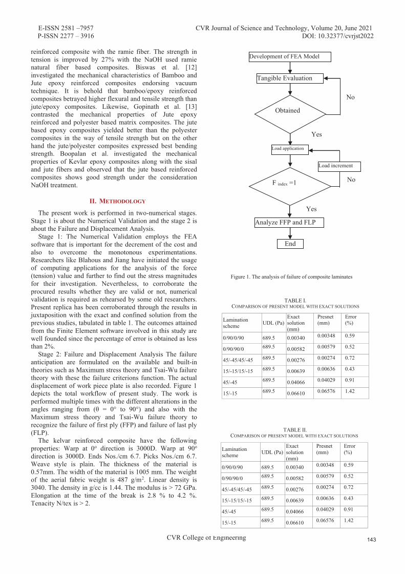
E-ISSN 2581 –7957 CVR Journal of Science and Technology, Volume 20, June 2021 P-ISSN 2277 – 3916 DOI: 10.32377/cvrjst2022
CVR College of Engineering
reinforced composite with the ramie fiber. The strength in tension is improved by 27% with the NaOH used ramie natural fiber based composites. Biswas et al. [12] investigated the mechanical characteristics of Bamboo and Jute epoxy reinforced composites endorsing vacuum technique. It is behold that bamboo/epoxy reinforced composites betrayed higher flexural and tensile strength than jute/epoxy composites. Likewise, Gopinath et al. [13] contrasted the mechanical properties of Jute epoxy reinforced and polyester based matrix composites. The jute based epoxy composites yielded better than the polyester composites in the way of tensile strength but on the other hand the jute/polyester composites expressed best bending strength. Boopalan et al. investigated the mechanical properties of Kevlar epoxy composites along with the sisal and jute fibers and observed that the jute based reinforced composites shows good strength under the consideration NaOH treatment.
II. METHODOLOGY
The present work is performed in two-numerical stages. Stage 1 is about the Numerical Validation and the stage 2 is about the Failure and Displacement Analysis.
Stage 1: The Numerical Validation employs the FEA software that is important for the decrement of the cost and also to overcome the monotonous experimentations. Researchers like Blahous and Jiang have initiated the usage of computing applications for the analysis of the force (tension) value and further to find out the stress magnitudes for their investigation. Nevertheless, to corroborate the procured results whether they are valid or not, numerical validation is required as rehearsed by some old researchers. Present replica has been corroborated through the results in juxtaposition with the exact and confined solution from the previous studies, tabulated in table 1. The outcomes attained from the Finite Element software involved in this study are well founded since the percentage of error is obtained as less than 2%.
Stage 2: Failure and Displacement Analysis The failure anticipation are formulated on the available and built-in theories such as Maximum stress theory and Tsai-Wu failure theory with these the failure criterions function. The actual displacement of work piece plate is also recorded. Figure 1 depicts the total workflow of present study. The work is performed multiple times with the different alterations in the angles ranging from (θ = 0° to 90°) and also with the Maximum stress theory and Tsai-Wu failure theory to recognize the failure of first ply (FFP) and failure of last ply (FLP).
The kelvar reinforced composite have the following properties: Warp at 0o direction is 3000D. Warp at 90o direction is 3000D. Ends Nos./cm 6.7. Picks Nos./cm 6.7. Weave style is plain. The thickness of the material is 0.57mm. The width of the material is 1005 mm. The weight of the aerial fabric weight is 487 g/m2. Linear density is 3040. The density in g/cc is 1.44. The modulus is > 72 GPa. Elongation at the time of the break is 2.8 % to 4.2 %. Tenacity N/tex is > 2.
Figure 1. The analysis of failure of composite laminates
TABLE I. COMPARISON OF PRESENT MODEL WITH EXACT SOLUTIONS
Lamination scheme UDL (Pa)
Exact solution (mm)
Presnet (mm)
Error (%)
0/90/0/90 689.5 0.00340 0.00348 0.59
0/90/90/0 689.5 0.00582 0.00579 0.52
45/-45/45/-45 689.5 0.00276 0.00274 0.72
15/-15/15/-15 689.5 0.00639 0.00636 0.43
45/-45 689.5 0.04066 0.04029 0.91
15/-15 689.5 0.06610 0.06576 1.42
Development of FEA Model
Tangible Evaluation
Obtained
Load application
F index =1
Load increment
Analyze FFP and FLP
End
Yes
Yes
No
No
TABLE II. COMPARISON OF PRESENT MODEL WITH EXACT SOLUTIONS
Lamination scheme UDL (Pa)
Exact solution (mm)
Presnet (mm)
Error (%)
0/90/0/90 689.5 0.00340 0.00348 0.59
0/90/90/0 689.5 0.00582 0.00579 0.52
45/-45/45/-45 689.5 0.00276 0.00274 0.72
15/-15/15/-15 689.5 0.00639 0.00636 0.43
45/-45 689.5 0.04066 0.04029 0.91
15/-15 689.5 0.06610 0.06576 1.42
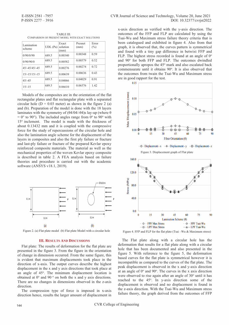
E-ISSN 2581 –7957 CVR Journal of Science and Technology, Volume 20, June 2021 P-ISSN 2277 – 3916 DOI: 10.32377/cvrjst2022
CVR College of Engineering
Models of the composites are in the orientation of the flat rectangular plates and flat rectangular plate with a separated circular hole (D = 0.03 meter) as shown in the figure 2 (a) and (b). Preparation of the model is done with the 18 layers laminates with the symmetry of (θ4/04/-θ4)s lay-up (where θ = 0° to 90°). The included angles range from 0o to 90o with 15o inclement. The model is made with the thickness of about 0.13432 mm and it is coupled with the compressive force for the study of repercussions of the circular hole and also the lamination angle scheme for the displacement of the layers in composites and also the first ply failure or fracture and last-ply failure or fracture of the prepared Kevlar epoxy reinforced composite materials. The material as well as the mechanical properties of the woven Kevlar epoxy composite is described in table 2. A FEA analysis based on failure theories and procedure is carried out with the academic software (ANSYS v18.1, 2019).
Figure 2. (a) Flat plate model (b) Flat plate Model with a circular hole
III. RESULTS AND DISCUSSIONS Flat plate: The results of deformation for the flat plate are
presented in the figure 3. From the figure in the orientation of change in dimension occurred. From the same figure, this is evident that maximum displacements took place in the direction of x-axis. The output curves describe the highest displacement in the x and y axis directions that took place at an angle of 45o. The minimum displacement location is obtained at 0o and 90 o on both the x and y axis directions. There are no changes in dimensions observed in the z-axis direction.
The compression type of force is imposed in x-axis direction hence, results the larger amount of displacement in
x-axis direction as verified with the y-axis direction. The outcomes of the FFP and FLP are calculated by using the Tsai-Wu and Maximum stress failure theory criteria that is been catalogued and exhibited in figure 4. Also from that graph, it is observed that, the curves pattern is symmetrical and found with a tiny gap difference in betwixt FFP and FLP. The highest stress recorded is found at an angle of 0o and 90o for both FFP and FLP. The outcomes dwindled proportionally apropos the 45o mark and also escalated back commensurate until it obtains 90o. It is also observed that the outcomes from twain the Tsai-Wu and Maximum stress are in good rapport for the test.
Figure 3. Displacement graph of Flat plate
Figure 4. FFP and FLP for the flat plate (Tsai –Wu & Maximum stress) The Flat plate along with a circular hole has the
deformation that results for a flat plate along with a circular hole that has been documented and also presented in the figure 5. With reference to the figure 5, the deformation based curves for the flat plate is symmetrical however it is incompatible as compared to the curves of the flat plate. The peak displacement is observed in the x and y-axis direction at an angle of 0o and 90o. The curves in the x axis direction were observed to rise again after an angle of 30o until it has reached to the 45o. In y-axis direction some of the displacement is observed and no displacement is found in the z-axis direction. With the Tsai-Wu and Maximum stress failure theory, the graph derived from the outcomes of FFP
TABLE III. COMPARISON OF PRESENT MODEL WITH EXACT SOLUTIONS
Lamination scheme UDL (Pa)
Exact solution (mm)
Presnet (mm)
Error (%)
0/90/0/90 689.5 0.00340 0.00348 0.59
0/90/90/0 689.5 0.00582 0.00579 0.52
45/-45/45/-45 689.5 0.00276 0.00274 0.72
15/-15/15/-15 689.5 0.00639 0.00636 0.43
45/-45 689.5 0.04066 0.04029 0.91
15/-15 689.5 0.06610 0.06576 1.42
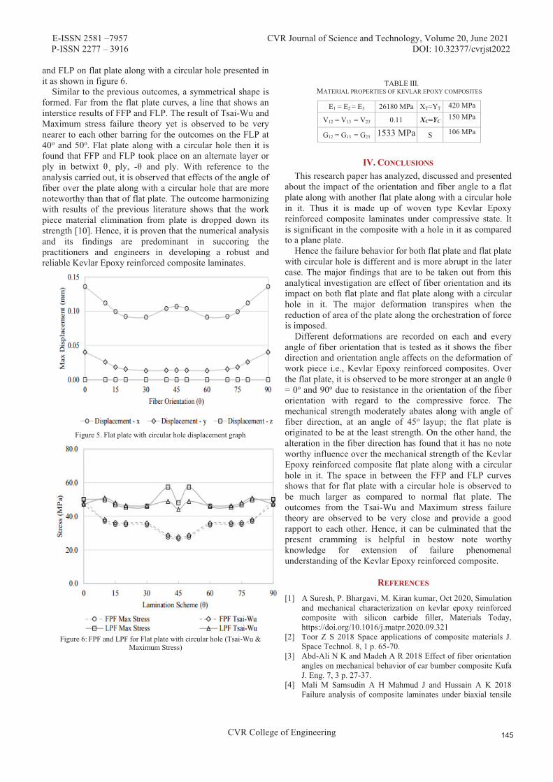
E-ISSN 2581 –7957 CVR Journal of Science and Technology, Volume 20, June 2021 P-ISSN 2277 – 3916 DOI: 10.32377/cvrjst2022
CVR College of Engineering
and FLP on flat plate along with a circular hole presented in it as shown in figure 6.
Similar to the previous outcomes, a symmetrical shape is formed. Far from the flat plate curves, a line that shows an interstice results of FFP and FLP. The result of Tsai-Wu and Maximum stress failure theory yet is observed to be very nearer to each other barring for the outcomes on the FLP at 40o and 50o. Flat plate along with a circular hole then it is found that FFP and FLP took place on an alternate layer or ply in betwixt θ ̧ ply, -θ and ply. With reference to the analysis carried out, it is observed that effects of the angle of fiber over the plate along with a circular hole that are more noteworthy than that of flat plate. The outcome harmonizing with results of the previous literature shows that the work piece material elimination from plate is dropped down its strength [10]. Hence, it is proven that the numerical analysis and its findings are predominant in succoring the practitioners and engineers in developing a robust and reliable Kevlar Epoxy reinforced composite laminates.
Figure 5. Flat plate with circular hole displacement graph
Figure 6: FPF and LPF for Flat plate with circular hole (Tsai-Wu &
Maximum Stress)
IV. CONCLUSIONS This research paper has analyzed, discussed and presented
about the impact of the orientation and fiber angle to a flat plate along with another flat plate along with a circular hole in it. Thus it is made up of woven type Kevlar Epoxy reinforced composite laminates under compressive state. It is significant in the composite with a hole in it as compared to a plane plate.
Hence the failure behavior for both flat plate and flat plate with circular hole is different and is more abrupt in the later case. The major findings that are to be taken out from this analytical investigation are effect of fiber orientation and its impact on both flat plate and flat plate along with a circular hole in it. The major deformation transpires when the reduction of area of the plate along the orchestration of force is imposed.
Different deformations are recorded on each and every angle of fiber orientation that is tested as it shows the fiber direction and orientation angle affects on the deformation of work piece i.e., Kevlar Epoxy reinforced composites. Over the flat plate, it is observed to be more stronger at an angle θ = 0o and 90o due to resistance in the orientation of the fiber orientation with regard to the compressive force. The mechanical strength moderately abates along with angle of fiber direction, at an angle of 45o layup; the flat plate is originated to be at the least strength. On the other hand, the alteration in the fiber direction has found that it has no note worthy influence over the mechanical strength of the Kevlar Epoxy reinforced composite flat plate along with a circular hole in it. The space in between the FFP and FLP curves shows that for flat plate with a circular hole is observed to be much larger as compared to normal flat plate. The outcomes from the Tsai-Wu and Maximum stress failure theory are observed to be very close and provide a good rapport to each other. Hence, it can be culminated that the present cramming is helpful in bestow note worthy knowledge for extension of failure phenomenal understanding of the Kevlar Epoxy reinforced composite.
REFERENCES
[1] A Suresh, P. Bhargavi, M. Kiran kumar, Oct 2020, Simulation and mechanical characterization on kevlar epoxy reinforced composite with silicon carbide filler, Materials Today, https://doi.org/10.1016/j.matpr.2020.09.321
[2] Toor Z S 2018 Space applications of composite materials J. Space Technol. 8, 1 p. 65-70.
[3] Abd-Ali N K and Madeh A R 2018 Effect of fiber orientation angles on mechanical behavior of car bumber composite Kufa J. Eng. 7, 3 p. 27-37.
[4] Mali M Samsudin A H Mahmud J and Hussain A K 2018 Failure analysis of composite laminates under biaxial tensile
TABLE III. MATERIAL PROPERTIES OF KEVLAR EPOXY COMPOSITES
E1 = E2 = E3 26180 MPa XT=YT 420 MPa
V12 = V13 = V23 0.11 XC=YC 150 MPa
G12 = G13 = G23 1533 MPa S 106 MPa

E-ISSN 2581 –7957 CVR Journal of Science and Technology, Volume 20, June 2021 P-ISSN 2277 – 3916 DOI: 10.32377/cvrjst2022
CVR College of Engineering
load due to variations in lamination scheme J. Mech. Eng. 13, 2 p. 10-20.
[5] Hashimoto M Okabe T Sasayama T Matsutani H and Nishikawa M 2018 Prediction of tensile strength of discontinous carbon fiber/polypropylene composite with fiber orientation distribution Compos. Part A. 43, p.1791-1799.
[6] Retnam B S J Sivapragash M and Pradeep P 2019 Effects of fibre orientation on mechanical properties of hybrid bamboo/glass fibre polymer composites Bull. Mater. Sci. 37, 5 p. 1059- 1064.
[7] Khusiafan F J 2018 Use of KEVLAR 49 in aircraft components Eng. Manage. Res. 7, 2 p. 14-19
[8] Talib A R A, Ramadhan A A, Rafie A S M and Zahari R 2018 Influence of cut-out hole on multilayer Kevlar-29/epoxy composite laminated plates Mater. Design. 43, p. 89-98.
[9] Nilakantan G and Gillespie Jr J W 2019 Yarn pull-out behavior of plain woven Kevlar fabrics: Effect of yarn sizin,
pullout rate, and fabric pre-tension Compos. Struct. 101, p. 215-224.
[10] Rahimi N Musa M Hussain A K and Mahmud J 2018 Finite element implementation to predict the failure of composite laminates under uniaxial tension Adv. Mater.Res. 499, p. 20-24.
[11] Jiang S and Blahous K 2020 Computer application in failure analysis of carbon/epoxy composite loops Inter. Conf.e on Edu. Technol.y and Comp. (ICETC). 2, p. 394-397.
[12] Samsudin A H and Mahmud J 2015 Deformation and failure analysis of symmetric and antisymmetric graphite/epoxy laminate due to variations in fiber orientation ARPN J. Eng. Appl. Sci. 10, 17 p. 7336-7344.
[13] Reddy J N 2012 Energy And Variational Methods In Applied Mechanics (with and Introduction to the Finite Element Method) (New York: John Wiley).

E-ISSN 2581 – 7957 CVR Journal of Science and Technology, Volume 20, June 2021 P-ISSN 2277 – 3916 DOI: 10.32377/cvrjst2023
CVR College of Engineering
Characterization of ZnO-TiO2 Hybrid Nano ased SAE 15W-40 Oil G. Naveen Kumar1 and G. Bharath reddy2
1Assoc. Prof., CVR College of Engineering/Mechanical Engg. Department, Hyderabad, India Email: [email protected]
2Asst. Prof., CVR College of Engineering/Mechanical Engg. Department, Hyderabad, India Email: [email protected]
Abstract: The main aim of the present investigation was to characterize the lubricant dispersed with ZnO-TiO2 hybrid nanoparticles. The work includes a dispersion of nanoparticles with varying proportions of 0.02 to 0.08 with an incremental step of 0.02 wt. % of base oil. Further, the samples were used to study the thermo-physical properties. The characterization result includes crystallinity and particle size of Zinc-oxide and titania nanoparticles, whereas the nano-based lubricant is characterized for its chemical compatibility, thermal conductivity, viscosity, and thermal stability. The result favors enhancing the thermo-physical properties of nano-based lubricant.
Index Terms: nanoparticles, lubricant, thermal conductivity.
I. INTRODUCTION
Organic lubricants are most popular in the various fields for operational enhancement. They can reduce friction between surfaces in mutual contact, ultimately reduces the heat generated when the surfaces move [1]. The property of reducing friction is known as lubricity. Typically, it also has additional functions of cooling the hotspots. Typically lubricants hold 90% base oil (mainly petroleum fractions, called mineral oils) and less than 10% additives. Synthetic liquids such as hydrogenated silicones, polyolefins, esters, fluorocarbons, and many others are sometimes used as base oils. Vegetable oils or synthetic liquids such as hydrogenated polyolefins, esters, silicones, fluorocarbons, and many others were sometimes used as base oils [2]. Additives can reduce friction and wear, increased viscosity, improved viscosity index, resistance to corrosion and oxidation, aging or contamination, etc. however, there is still much space for enhancing the thermo-physical properties of the lubricant.
The thermal conductivity of lubricants is an important factor in determining the cooling behavior; nevertheless, the low thermal conductivity of conventional lubricants confines their performance [14]. Researchers enhanced the thermal conductivity of lubricant with nano inclusions in it. Dispersed 7% Vol. fraction of ZrO2 nanoparticles, there was an appreciable enhancement of thermal conductivity. ZnO nanoparticles were dispersed in EG base fluid and achieved thermal conductivity enhancement of 9.13% [3]. Several researchers attempted enhancing the thermal conductivity of lubricant with nanoparticles dispersion. Nevertheless, hybrid
ZnO-TiO2 nanoparticles combination with SAE 15W-40 lubricant has not been tried for thermo-physical enhancement.
II. MATERIALS AND INSTRUMENTS
SAE 15W-40 lubricant procured from sigma Aldrich, Titanium dioxide, and Zinc Oxide nanoparticles were procured from Alfa Aesar, GT SONIC-QTD model for effective dispersion of nanoparticles in SAE 15W-40 lubricant. Rheometer instrument, HR 20 model, for measuring the viscosity of the sample, Fourier transform infrared spectroscopy to study the chemical compatibility of the sample, Thermogravimetric analyzer (TGA) SDT 650 model to study decomposition temperature of the sample, the thermal conductivity analyzer (TCA), FOX 200 model to measure thermal conductivity of the samples.
I I. METHODOLOGY
The conventional SAE 15W-40 lubricant was tested to thermo-physical characteristics; further ZnO-TiO2 nanoparticles were dispersed in the lubricant with varying from 0.02 to 0.08 with the incremental step of 0.02 wt. %. The agglomerated nanoparticles were ultrasonicated to de-agglomerate and to have a nano effect. The five samples (1 conventional lubricant and 4 nano based lubricant) were tested to study thermo-physical properties with an increased percentage of nanoparticles.
I . HYBRID NANO BASED OIL PREPARATION
The combined effect of ZnO and TiO2 nanoparticles were used in the oil for the preparation of hybrid nano-based oil. Table 1 shows the different samples. Sample 1 was the base oil without any nano effect, whereas the nanoparticles were dispersed in the oil varying from 0.02 to 0.08 weight percentage of oil with the increment of 0.02%.

E-ISSN 2581 – 7957 CVR Journal of Science and Technology, Volume 20, June 2021 P-ISSN 2277 – 3916 DOI: 10.32377/cvrjst2023
CVR College of Engineering
Figure 1. Pure and Hybrid nano based oil samples
TABLE I. HYBRID TITANIA - ZINCOXIDE BASED OIL PREPARATION
Sample No. Oil (ml) TiO2 (wt.
%) ZnO (wt.
%)
Total hybrid nano%
1 20 0 0 0 2 20 0.01 0.01 0.02 3 20 0.02 0.02 0.04 4 20 0.03 0.03 0.06 5 20 0.04 0.04 0.08
TABLE II. INSTRUMENT SPECIFICATION
S. No Instrument Purpose
1 Particle Size Analyzer Size of particles
2 Probe sonicator Nanoparticles dispersion in fluid
3 Fourier Transformer Infrared spectroscopy Chemical compatibility
4 Thermogravimetric analyzer Decomposition temperature
5 Rheometer Viscosity
6 Thermal conductivity Analyzer Thermal conductivity
. RESULTS AND DISCUSSIONS
A. Particle Size Analysis The nanoparticles were procured for dispersion in the oil
for preparing hybrid nano-based oil preparation; particle size analysis was performed to study the size distribution range. Figure 2 depicts that the particle range from 42 nm to 95 nm, and the average particle particles are around 70 nm with an intensity of almost 47%. There are traces of noise disturbances that can be seen in figure 2.
Figure 2. ZnO nano particle size distribution curve
Figure 3. TiO2 nano particle size distribution.
The TiO2 nanoparticles procured were used for nano oil preparation, and before using it, to confirm its particle range particle size analysis was done. The results depict that the particles range from 52 nm to almost 125 nm however, the average particle was close to 78 nm with an intensity of almost 50%. This confirms that the particles are nano range.
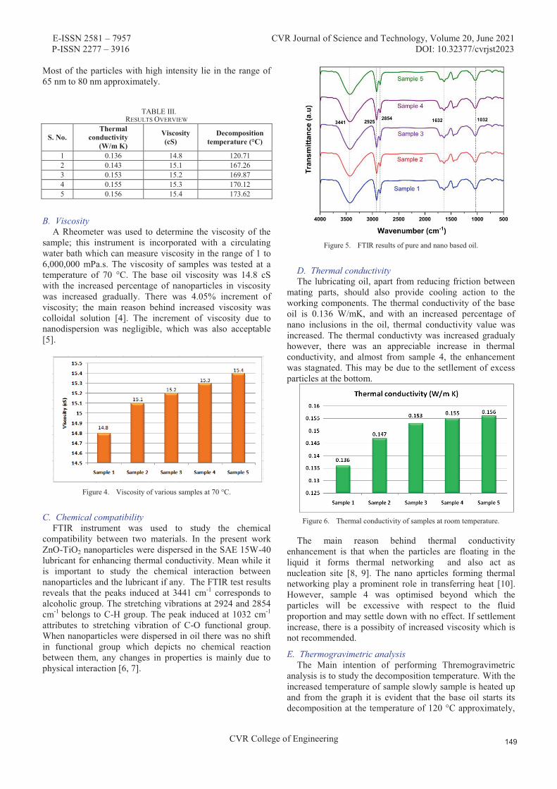
E-ISSN 2581 – 7957 CVR Journal of Science and Technology, Volume 20, June 2021 P-ISSN 2277 – 3916 DOI: 10.32377/cvrjst2023
CVR College of Engineering
Most of the particles with high intensity lie in the range of 65 nm to 80 nm approximately.
TABLE III. RESULTS OVERVIEW
S. No. Thermal
conductivity (W/m K)
Viscosity (cS)
Decomposition temperature (°C)
1 0.136 14.8 120.71 2 0.143 15.1 167.26 3 0.153 15.2 169.87 4 0.155 15.3 170.12 5 0.156 15.4 173.62
B. Viscosity A Rheometer was used to determine the viscosity of the
sample; this instrument is incorporated with a circulating water bath which can measure viscosity in the range of 1 to 6,000,000 mPa.s. The viscosity of samples was tested at a temperature of 70 °C. The base oil viscosity was 14.8 cS with the increased percentage of nanoparticles in viscosity was increased gradually. There was 4.05% increment of viscosity; the main reason behind increased viscosity was colloidal solution [4]. The increment of viscosity due to nanodispersion was negligible, which was also acceptable [5].
Figure 4. Viscosity of various samples at 70 °C.
C. Chemical compatibility FTIR instrument was used to study the chemical
compatibility between two materials. In the present work ZnO-TiO2 nanoparticles were dispersed in the SAE 15W-40 lubricant for enhancing thermal conductivity. Mean while it is important to study the chemical interaction between nanoparticles and the lubricant if any. The FTIR test results reveals that the peaks induced at 3441 cm-1 corresponds to alcoholic group. The stretching vibrations at 2924 and 2854 cm-1 belongs to C-H group. The peak induced at 1032 cm-1
attributes to stretching vibration of C-O functional group. When nanoparticles were dispersed in oil there was no shift in functional group which depicts no chemical reaction between them, any changes in properties is mainly due to physical interaction [6, 7].
Figure 5. FTIR results of pure and nano based oil.
D. Thermal conductivity The lubricating oil, apart from reducing friction between
mating parts, should also provide cooling action to the working components. The thermal conductivity of the base oil is 0.136 W/mK, and with an increased percentage of nano inclusions in the oil, thermal conductivity value was increased. The thermal conductivty was increased gradualy however, there was an appreciable increase in thermal conductivity, and almost from sample 4, the enhancement was stagnated. This may be due to the setllement of excess particles at the bottom.
Figure 6. Thermal conductivity of samples at room temperature.
The main reason behind thermal conductivity enhancement is that when the particles are floating in the liquid it forms thermal networking and also act as nucleation site [8, 9]. The nano aprticles forming thermal networking play a prominent role in transferring heat [10]. However, sample 4 was optimised beyond which the particles will be excessive with respect to the fluid proportion and may settle down with no effect. If settlement increase, there is a possibity of increased viscosity which is not recommended.
E. Thermogravimetric analysis The Main intention of performing Thremogravimetric
analysis is to study the decomposition temperature. With the increased temperature of sample slowly sample is heated up and from the graph it is evident that the base oil starts its decomposition at the temperature of 120 °C approximately,
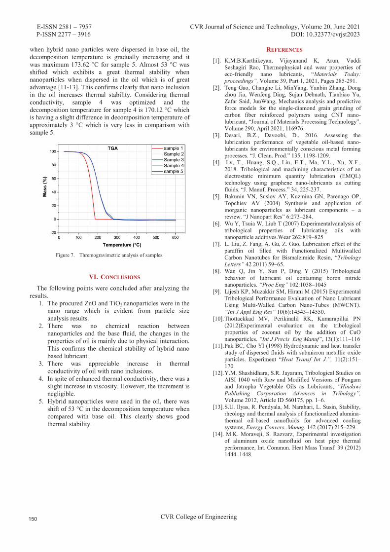
E-ISSN 2581 – 7957 CVR Journal of Science and Technology, Volume 20, June 2021 P-ISSN 2277 – 3916 DOI: 10.32377/cvrjst2023
CVR College of Engineering
when hybrid nano particles were dispersed in base oil, the decomposition temperature is gradually increasing and it was maximum 173.62 °C for sample 5. Almost 53 °C was shifted which exhibits a great thermal stability when nanoparticles when dispersed in the oil which is of great advantage [11-13]. This confirms clearly that nano inclusion in the oil increases thermal stability. Considering thermal conductivity, sample 4 was optimized and the decomposition temperature for sample 4 is 170.12 °C which is having a slight difference in decomposition temperature of approximately 3 °C which is very less in comparison with sample 5.
Figure 7. Thremogravimetric analysis of samples.
V . CONCLUSIONS
The following points were concluded after analyzing the results.
1. The procured ZnO and TiO2 nanoparticles were in thenano range which is evident from particle sizeanalysis results.
2. There was no chemical reaction betweennanoparticles and the base fluid, the changes in theproperties of oil is mainly due to physical interaction.This confirms the chemical stability of hybrid nanobased lubricant.
3. There was appreciable increase in thermalconductivity of oil with nano inclusions.
4. In spite of enhanced thermal conductivity, there was aslight increase in viscosity. However, the increment isnegligible.
5. Hybrid nanoparticles were used in the oil, there wasshift of 53 °C in the decomposition temperature whencompared with base oil. This clearly shows goodthermal stability.
REFERENCES [1]. K.M.B.Karthikeyan, Vijayanand K, Arun, Vaddi
Seshagiri Rao, Thermophysical and wear properties of eco-friendly nano lubricants, “Materials Today: proceedings”, Volume 39, Part 1, 2021, Pages 285-291.
[2]. Teng Gao, Changhe Li, MinYang, Yanbin Zhang, Dong zhou Jia, Wenfeng Ding, Sujan Debnath, Tianbiao Yu, Zafar Said, JunWang, Mechanics analysis and predictive force models for the single-diamond grain grinding of carbon fiber reinforced polymers using CNT nano-lubricant, “Journal of Materials Processing Technology”, Volume 290, April 2021, 116976.
[3]. Desari, B.Z., Davoobi, D., 2016. Assessing the lubrication performance of vegetable oil-based nano-lubricants for environmentally conscious metal forming processes. “J. Clean. Prod.” 135, 1198-1209.
[4]. Lv, T., Huang, S.Q., Liu, E.T., Ma, Y.L., Xu, X.F., 2018. Tribological and machining characteristics of an electrostatic minimum quantity lubrication (EMQL) technology using graphene nano-lubricants as cutting fluids. “J. Manuf. Process.” 34, 225-237.
[5]. Bakunin VN, Suslov AY, Kuzmina GN, Parenago OP, Topchiev AV (2004) Synthesis and application of inorganic nanoparticles as lubricant components – a review. “J Nanopart Res” 6:273–284.
[6]. Wu Y, Tsuia W, Liub T (2007) Experimentalvanalysis of tribological properties of lubricating oils with nanoparticle additives.Wear 262:819–825
[7]. L. Liu, Z. Fang, A. Gu, Z. Guo, Lubrication effect of the paraffin oil filled with Functionalized Multiwalled Carbon Nanotubes for Bismaleimide Resin, “Tribology Letters” 42 2011) 59–65.
[8]. Wan Q, Jin Y, Sun P, Ding Y (2015) Tribological behavior of lubricant oil containing boron nitride nanoparticles. “Proc Eng” 102:1038–1045
[9]. Lijesh KP, Muzakkir SM, Hirani M (2015) Experimental Tribological Performance Evaluation of Nano Lubricant Using Multi-Walled Carbon Nano-Tubes (MWCNT). “Int J Appl Eng Res” 10(6):14543–14550.
[10]. Thottackkad MV, Perikinalil RK, Kumarapillai PN (2012)Experimental evaluation on the tribological properties of coconut oil by the addition of CuO nanoparticles. “Int J Precis Eng Manuf”, 13(1):111–116
[11]. Pak BC, Cho YI (1998) Hydrodynamic and heat transfer study of dispersed fluids with submicron metallic oxide particles. Experiment “Heat Transf Int J.”, 11(2):151–170
[12]. Y.M. Shashidhara, S.R. Jayaram, Tribological Studies on AISI 1040 with Raw and Modified Versions of Pongam and Jatropha Vegetable Oils as Lubricants, “Hindawi Publishing Corporation Advances in Tribology”, Volume 2012, Article ID 560175, pp. 1–6.
[13]. S.U. Ilyas, R. Pendyala, M. Narahari, L. Susin, Stability, rheology and thermal analysis of functionalized alumina-thermal oil-based nanofluids for advanced cooling systems, Energy Convers. Manag. 142 (2017) 215–229.
[14]. M.K. Moraveji, S. Razvarz, Experimental investigation of aluminum oxide nanofluid on heat pipe thermal performance, Int. Commun. Heat Mass Transf. 39 (2012) 1444–1448.
E-ISSN 2581 – 7957 CVR Journal of Science and Technology, Volume 20, June 2021 P-ISSN 2277 – 3916 DOI: 10.32377/cvrjst2024
CVR College of Engineering
Synthesis of 1, 8-Naphthyridine Derivatives using Biodegradable Starch Sulfuric Acid as
Heterogeneous Catalyst Kadeer Md1, Dr. Ramakanth Pagadala2, Dr. Venkatesan Kasi3 and Dr. Ramesh Domala4 1Asst. Professor, CVR College of Engineering/H&S Department (Chemistry), Hyderabad, India
Email: [email protected] 2 Asst. Professor, CVR College of Engineering/H&S Department (Chemistry), Hyderabad, India
Email: [email protected] 3Asst. Professor, CVR College of Engineering/H&S Department (Chemistry), Hyderabad, India
Email: [email protected] 4Asst. Professor, Department of Chemistry and Pharmaceutical Sciences, M G University, Nalgonda, India
Email: [email protected]
Abstract: 2-amino-3-cyano substituted 1,8-naphthyridines has been developed in the presence of starch sulfuric acid (SSA catalyst using aminopyridine, malononitrile, and aromatic aldehydes via Knoevenagel condensation and Michael addition followed by intramolecular cyclization. The SSA catalyst could selectively be converted amino pyridine into 1,8-naphthyridines with good yield in a short period of time at room temperature. This catalyst can be efficiently reused several times without loss of its sustainable activity.
Index Terms: Starch sulfuric acid, naphthyridines, biodegradable solid catalyst, heterogeneous acid catalyst
I. INTRODUCTION
Greener synthetic transformations in the synthesis of bioactive heterocyclic compounds under solvent-free conditions provide more advantageous to the research laboratories and pharmaceutical industry [1-3]. Green chemical methodologies have become the motivating strength for organic researchers to afford environmentally kind paths for the synthesis of heterocyclic compounds. Hence, the enhancement of these privileged biologically important organic compounds in a greater yield of products in shorter process time, and from easily obtainable starting materials in great demand. The objective of green chemistry is to eliminate the hazardous byproducts, prevention of waste and increase the yield of the target compound with a sustainable eco-friendly environment [4, 5]. Bio-degradable catalysts had developed various environmentally benign protocols for organic synthesis [6-8]. Multicomponent one pot synthesis has great profit to the pharmaceutical industry with design and synthesis of organic molecules, where it can minimize time, cost and energy [9].
Heterocyclic compounds have a distinct place among pharmaceutically significant natural products and synthetic organic compounds [10-12]. Nitrogen heterocyclic compounds are abundant in nature and are of great importance to human life as they exist in many natural products such as alkaloids, hormones and vitamins [13-16]. The construction of naphthyridine analogs are huge importance in pharmacological, bio medicinal and synthetic chemistry.
The synthesis of nitrogenous aromatic substituted compounds such as 1,8-naphthyridine moieties has magnificent significance in medicinal research. Substituted 1,8-naphthyridines have attracted considerable attention to fertile field of research due to its various biological activities such as antimicrobial [17], antimalarial [18], anti-inflammatory [19, 20], anticonvulsant [21], hypoglycemic [22], vasodilators [23], psychotropic properties [24], insecticide [25] muscle relaxant [26] anticancer [27], β-adrenergic blocking properties [28], anti-hypertensive [29]. In previous years, nucleophilic substitution reactions were extensively used for the synthesis of substituted 1,8-naphthyridine catalyzed by CoCl2 in THF, N,N,N′,N′-tetrabromobenzene-1,3-disulfonamide [30] and various multi step catalyzed compounds which have more disadvantages like the toxicity of reagents, long reaction time, harsh reaction conditions such as high reaction temperatures, expensive, most of the reactions require tedious work-up procedures and recyclability of catalyst. Therefore, there is a need to develop a more efficient, simple and convenient protocol using a conservation catalyst.
Recently, the research being focused on the starch sulfuric acid (SSA) as solid heterogeneous catalyst due to its unique properties such as more efficient, economical, compatible and eco-friendly. The present study is intended to the synthesis of poly functional substituted 1,8-naphthyridines using SSA as heterogeneous catalyst.
II. RESULTS AND DISCUSSION
SSA is prepared by the addition of drop wise 0.5 g of chlorosulfonic acid (4.5 mmol) to the 2.5 grams of starch and added for about 10 ml of n-hexane at 0oC (Figure 1). Stirred the solution for about 2 hours and filter the compound. This SSA is white colored, non-hygroscopic solid and stable under reaction conditions.
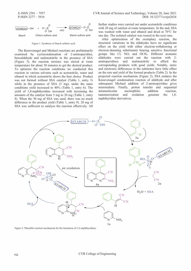
E-ISSN 2581 – 7957 CVR Journal of Science and Technology, Volume 20, June 2021 P-ISSN 2277 – 3916 DOI: 10.32377/cvrjst2024
CVR College of Engineering
Figure 1. Synthesis of Starch sulfuric acid.
The Knoevenagel and Michael reactions are preliminarily
examined by cyclocondensation of 2-aminopyridine, benzaldehyde and malononitrile in the presence of SSA (Figure 3), the reaction mixture was stirred at room temperature for about 30 minutes to get the desired product. To optimize the reaction conditions we conducted this reaction in various solvents such as acetonitrile, water and ethanol in which acetonitrile shows the best choice. Product was not formed without SSA catalyst (Table 1, entry 3) while in the presence of SSA (5 mg), under the same conditions yield increased to 40% (Table 1, entry 6). The yield of 1,8-naphthyridine increased with increasing the amounts of the catalyst from 5 mg to 20 mg (Table 1, entry 8). When the 30 mg of SSA was used, there was no much difference in the product yield (Table 1, entry 9). 20 mg of SSA was sufficient to catalyze the reaction effectively. All
further studies were carried out under acetonitrile conditions with 20 mg of catalyst at room temperature. In the end, SSA was washed with water and ethanol and dried at 70°C for one day. The isolated catalyst was reused in the next runs.
After optimization of the exemplary reaction, the structural variations in the aldehydes have no significant effect on the yield with either electron-withdrawing or electron-donating substituents bearing sensitive functional groups like Cl, NO2 and OCH3. Different aromatic aldehydes were carried out the reaction with 2-aminopyridines and malononitrile to afford the corresponding products with good yields. Notably, steric and electronic differences in the substrates have little effect on the rate and yield of the formed products (Table 2). In the projected reaction mechanism (Figure 2), SSA endures the Knoevenagel condensation reaction of aldehyde and after subsequent Michael addition of 2-aminopyridine gives intermediate. Finally, proton transfer and sequential intramolecular nucleophilic addition reaction, tautomerization and oxidation generate the 1,8-naphthyridine derivatives.
Figure 2. Plausible reaction mechanism for the formation of 1,8-naphthyridines

E-ISSN 2581 – 7957 CVR Journal of Science and Technology, Volume 20, June 2021 P-ISSN 2277 – 3916 DOI: 10.32377/cvrjst2024
CVR College of Engineering
Figure 3. SSA catalyzed synthesis of the 1,8-Naphthyridines (4a-h).
III. EXPERIMENTAL
Typical procedure for the synthesis of 1,8-naphthyridine derivatives catalyzed by SSA (4a-h)
A mixture of 2-aminopyridine (1 mmol), malononitrile (1 mmol), benzaldehyde (1.2 mmol), and SSA catalyst (20 mg) in acetonitrile (5 mL) was stirred at room temperature for the appropriate length of time (Table 1, entry 6). The progress of the reaction was monitored by TLC (6:4, n-hexane/ethyl acetate). After completion of the reaction, acetonitrile (10 mL) was added. The solid was filtered, washed with acetonitrile and dried. The residue was recrystallized from ethanol to afford the pure product. After evaporation of acetonitrile by reduced pressure, dichloromethane was added and filtered the catalyst. The collected SSA catalyst was reused four times in the same reaction.
Product 4a Off-white solid, Mp. 149-152 oC; IR (νmax, cm-1) (KBr): 3249, 3329, 2219; NMR 1H (300 MHz, CDCl3): δ 7.09 (s, 2H, NH2), 7.14 (m, 1HAr), 7.17 (m, 2HAr), 7.20 (m, 2HAr), 7.24 (m, 1HAr), 7.26 (m, 1HAr), 7.28 (m, 1HAr); C-13 NMR (100 MHz, CDCl3): δ117.8, 119.1, 124.2, 126.4, 127.8, 128.6, 129.5, 132.2, 136.1, 138.9, 143.5, 154.4, 158.9, 169.9, 172.5; EIMS: (m/z): 242 (M+1); Anal. Theoretical for C15H10N4: C; 73.16, H; 4.09, N; 22.75. Found (Exp.): C; 73.20, H; 4.10, N; 22.79.
Product 4b
TABLE II. SYNTHESIS OF 1,8-NAPHTHYRIDINES
ENTRY Aldehyde Product Time Yield (%)
1
3a
4a
30min 85
2
3b
4b
30min 81
3
3c
4c
30min 80
4
3d
4d
30min 82
5
3e
4e
30min 76
6
3f 4f
30min 83
7
3g 4g
30min 76
8
3h4h
30min 78
a Isolated yields
TABLE I. EFFECT OF SOLVENT ON SYNTHESIS OF 1,8-NAPHTHYRIDINES
ENTRY Compound
Amount
Solvent Temp Time Yield a(%)
1 4a - Ethanol rt 6h b
2 4a - Ethanol 70oC 6h b
3 4a - Acetonitrile rt 6h b
4 4a - Water rt 6h b
5 4a - Water 80oC 6h b
6 4a 5mg Acetonitrile rt 6h 40
7 4a 20mg Water rt 4h b
8 4a 20mg Acetonitrile rt 30min 85
9 4a 30mg Acetonitrile rt 30min 84
rt: room temperature; a Isolated yields; b No product found

E-ISSN 2581 – 7957 CVR Journal of Science and Technology, Volume 20, June 2021 P-ISSN 2277 – 3916 DOI: 10.32377/cvrjst2024
CVR College of Engineering
Off-white solid, Mp. 158-160 oC; IR (νmax, cm-1) (KBr): 3263, 3325,2223; NMR 1H (300 MHz, CDCl3): δ 7.13 (s, 2H, NH2), 7.18 (m, 2HAr), 7.24 (m, 2HAr), 7.29 (m, 1HAr), 7.30 (m, 1HAr), 7.36 (m, 1HAr); C-13 NMR (100 MHz, CDCl3): δ 110.8, 113.9, 116.4, 118.2, 121.2, 125.1, 128.2, 132.6, 135.9, 139.1, 141.8, 146.8, 147.6, 151.2, 155.5, 164.1; EMIS: (m/z): 292.32 (M+1) Anal. Theoretical for C15H9N5O2: C; 61.85, H; 3.11, N; 24.04, O; 10.99. Found (Exp.): C; 61.71, H; 3.10, N; 24.05, O; 10.96. Product 4c Off-white solid; NMR 1H (300 MHz, CDCl3): δ 4.21 (s, 3H), 5.58 (s, 2H), 6.11(s, 1H), 6.61 (d, 1H), 6.70 (d, 1H), 7.17 (d,1H), 7.78 (m, 3H), C-13 NMR (100 MHz, CDCl3): δ 62.5, 88.4, 115.0, 117.8, 118.9, 121.7, 125.1, 128.7, 132.8, 135.6, 138.8, 141.4, 146.6, 149.3, 154.9, 164.5. EMIS: (m/z): 293.16 [M+]; Anal. Theoretical for C16H12N4O2: C; 65.75, H; 4.14, N; 19.17, O; 10.95. Found (Exp.): C; 65.74, H; 4.09, N; 19.15, O; 10.96. Product 4d Off-white solid Mp. 155-157 oC; IR (νmax, cm-1) (KBr): 3240, 3292, 2231; NMR 1H (300 Hz, CDCl3): δ 3.749 (s, 3H), 6.81 (m, 2H, HAr), 7.21 (m, 1H, ArH), 7.29 (m, 1H, ArH), 7.31 (s, 2H, NH2), 7.37 (m, 2H, ArH), 7.40 (m, 1H, ArH); C-13 NMR (100 MHz, CDCl3): δ 111.9, 117.0, 121.6, 123.4, 125.0, 128.1, 130.1, 134.2, 135.8, 141.8, 145.9, 147.1, 150.3, 151.8, 158.1, 168.0; EIMS: (m/z): 261 (M+). Anal. Theoretical for C16H12N4: C; 73.83, H; 4.65, N; 21.52. Found (Exp.): C; 73.80, H; 4.63, N; 21.48.
Product 4e Yellow solid, Mp. 159-161 oC; IR (νmax, cm-1) (KBr): 3247, 3309, 2231; NMR 1H (400 MHz, CDCl3): δ 7.16 (s, 2H, NH2), 7.21 (s, 1H, ArH), 7.23 (m, 1H, ArH), 7.24 (m, 1H, ArH), 7.27 (m, 1H, ArH), 7.30 (m, 1HAr),7.33 (m, 1H, ArH), 7.36 (m, 1H, ArH); C-13 NMR (100 MHz, CDCl3): δ 111.1, 111.9, 113.4, 117.8, 122.0, 124.5, 128.8, 134.0, 136.1, 138.9, 142.0, 147.0, 149.0, 151.1, 155.0, 165.1; EIMS: (m/z): 291.41 (M+). Anal. Theoretical for C15H9N5O2: C; 61.85, H; 3.11, N; 24.04, O; 10.99. Found: C; 69.82, H; 3.11, N; 24.01, O; 11.01. Product 4f Orange solid; mp 164-167 oC; IR (νmax, cm-1) (KBr) 3423, 3056, 2176, 1634, 1618, 1601, 1539, 1459, 1363, 1268, 1143, 1087; NMR 1H (300 MHz, CDCl3): δ 6.92-7.47 (m, 3H, ArH), 8.62 (s, 1H, ArH), 8.67 (s, 1H, ArH), 7.73 (d, 2H, NH2), δ 3.34 (s, 1H, OH); C-13 NMR (100 MHz, CDCl3): δ: 113.7, 114.3, 119.2, 121.8, 129.4, 136.6, 142.2, 151.1, 154.6, 159.8, 161.8. EIMS: (m/z): 420.06 (M+3) Anal. Theoretical for C15H8Br2N4O: C; 42.89.16, H; 1.89, N; 13.84. Found (Exp.): C; 43.10, H; 1.87, N; 13.79. Product 4g Off-white solid; mp 164-166 oC; IR (νmax, cm-1) (KBr) 3434, 3092, 1725, 1689, 1604, 1576, 1543, 1434, 1423, 1296, 1214, 1178, 1109; NMR 1H (300 MHz, CDCl3): δ 7.56 (d, 2H, NH2), 7.75 (s, 1H, ArH), 7.43 (d, J = 7.2Hz, 1H, ArH), 7.56(d, J = 6.2Hz, 1H, ArH), 8.59 (s, 1H, ArH),
8.63 (s, 1H, ArH); C-13 NMR (100 MHz, CDCl3): δc: 119.7, 121.6, 126.9, 129.0, 131.7, 132.9, 134.3, 134.5, 135.1, 135.7, 138.6, 139.4, 140.6, 142.1, 151.2,159.8, 160.1, 162.5. EIMS: (m/z): 394 (M+), Anal. Theoretical for C15H7BrCl2N4: C; 45.72.16, H; 1.79, N; 14.22. Found (Exp.): C; 45.67, H; 1.80, N; 14.18. Product 4h Orange solid; mp 167-169 oC; IR (νmax, cm-1) (KBr) 3423, 3312, 3009, 2957, 1728, 1678, 1608, 1578, 1472, 1266, 1217, 1090, 865; NMR 1H (300 MHz, CDCl3): δ 3.27 (s, 1H, OH), 3.59 (s, 3H, OCH3), 7.71 (s, 2H, NH2), 6.76 (t, J = 5.0 Hz, 1H, ArH), 6.84 (d, J = 6.1 Hz, 1H, ArH), 7.07-7.21 (m, 3H, ArH), 7.89 (t, J = 3.3 Hz, 1H, ArH); C-13 NMR (100 MHz, CDCl3): δ 54.8, 57.3, 109.2, 112.7, 115.4, 118.7, 120.3, 121.4, 123.5, 124.3, 125.3, 138.2, 140.1, 146.9, 149.4, 149.7, 158.7, 163.2. EIMS: (m/z): 292.2 (M+), Anal. Theoretical for C16H12O2N4: C; 65.75.16, H; 4.14, N; 19.17. Found (Exp.): C; 65.76, H; 4.10, N; 19.09.
IV. CONCLUSIONS
In summary, we have synthesized a simple and effective method for the synthesis of medicinally important 2-amino 3-cyano substituted 1,8-naphthyridine derivatives. The SSA a catalyst reported in this paper will contribute positively to the green synthetic process by reducing the use of organic solvents. Catalytic amount of heterogeneous catalyst can be easily recovered and reutilized. The proposed method offers eco-friendly and reutilized SSA catalyst with easily available starting materials. In the view of ecological criteria, the present protocol should be a valuable addition for the synthesis of 2-amino 3-cyano substituted 1,8-naphthyridines.
REFERENCES [1] G. L. Thomas, R. J. Spandl, F. G. Glansdorp, M. Welch, A.
Bender, J. Cockfield, J. A. Lindsay, C. Bryant, D. F. J. Brown, O. Loiseleur, H. Rudyk, M. Ladlow, D. R. Spring, Angew. Chem. Int. Ed., 2008, 47, 2808.
[2] A. E. Rosamilia, C. R. Strauss, J. L. Scott, Pure Appl. Chem. 2007, 79, 1869.
[3] J. M. Mitchell, J. T. Shaw, Angew. Chem. Int. Ed. 2006, 45, 1722.
[4] M. B. Gawande, V. D. B. Bonifacio, R. Luque, P. S. Brancoa and R. S. Varma, Chem. Soc. Rev., 2013, 42, 5522.
[5] M. B. Gawande, P. S. Branco and R. S. Varma, Chem. Soc. Rev., 2013, 42, 3371.
[6] R. Ramachandran, S. Jayanthi, Y. T. Jeong, Tetrahedron., 2012, 68, 363.
[7] R. G. Koduri1, R. Pagadala1, R. Varala, CVR Journal of Science and Technology, 2018, 14, 107.
[8] M. D. Carrigan, K. J. Eash, M. C. Oswald, R. S. Mohan, Tetrahedron Lett., 2001, 42, 8133.
[9] J. C. Wasilke, S. J. Obrey, R. Tom Baker and G. C. Bazan, Chem. Rev., 2005, 105, 1001.
[10] R. Pagadala, S. Maddila, S. Rana, S.B. Jonnalagadda., RSC Adv., 2014, 4, 6602.
[11] R. Pagadala, S. Maddila, S.B. Jonnalagadda, Green Chem. Lett. Rev., 2014, 7, 131.
[12] Dr. K. Venkatesan, Dr. P. Ramakanth, Dr. Ch. Anjaneyulu, CVR Journal of Science and Technology, 2020, 18, 144.

E-ISSN 2581 – 7957 CVR Journal of Science and Technology, Volume 20, June 2021 P-ISSN 2277 – 3916 DOI: 10.32377/cvrjst2024
CVR College of Engineering
[13] R. Pagadala, S. Maddila, S. B. Jonnalagadda, Ultrasonics Sonochem., 2014, 21, 472.
[14] R. Pagadala, S. Maddila, V.D.B.C. Dasireddy, S.B. Jonnalagadda, Catal. Commun., 2014, 45, 148.
[15] R. Pagadala, S. Maddila, S.B. Jonnalagadda, Org. Prep. Proc. Int., 2014, 46, 261.
[16] R. Pagadala, S. Maddila, V. Moodley, W.E. van Zyl, S. B. Jonnalagadda, Tetrahedron Lett., 55 (2014) 4006.
[17] F. A. Ashour, S. A. Al-Mazoroa, J Pharm Sci., 1990, 4, 29. [18] P. Melnyk, V. Leroux, C. Sergheraert, P. Grellier, Bioorg.
Med. Chem. Lett., 2006, 16, 31. [19] M. Amir, S. Shahani, Indian J Heterocyclic Chem., 1998, 8,
107. [20] R. Paprocka, M. Wiese, A. Eljaszewicz, A. Helmin-Basa, A.
Gzella, B. Modzelewska-Banachiewicz, J. Michalkiewicz, Bioorg. Med. Chem. Lett., 2015, 25, 2664.
[21] J. R. Dimmock, S. C. Vashishtha, J. P. Stables, Eur. J. Med. Chem., 2000, 35, 241.
[22] F. Kurzer, Org. Compd. Sulphur Selenium Tellurium, 1974, 4, 417.
[23] L. C. Cullen, S. H. Lalgudi, D. D. Feng Chi, P. Ashok, J. Comb. Chem. 2008, 10, 28.
[24] M. K. Khalid, S. Salman, S. Muhammad, T. Muhammad, M. S. Syed, P. Shahnaz, M. Iqbal Choudhar, Bioorg. Med. Chem., 2014, 22, 6509.
[25] A. A. Fadda, E. M. Afsah, S. Bondock, M. M. Z. Hammouda, B. Naturforsch, J. Chem. Sci., 2015, 70, 385.
[26] M. H. Sherlock, J. J. Kaminsky, W. C. Tom, J. F. Lee, S. C. Wong, R. W. Bryant, A. T. McPhail, J. Med. Chem. 1988, 31, 2108.
[27] P. L. Ferrarini, C. Mori, G. Biogi, O. Livi, I. Tonetti, J. Heterocyclic Chem., 1984, 21, 417.
[28] P. L. Ferrarini, C. Mori, M. Badawneh, V. Calderone, R. Greco, C. Manera, A. Martinelli, P. Nieri, G. Saccomanni, Eur. J. Med. Chem., 2000, 35, 815.
[29] M. Ferrarini, M. Clendio, U. Calder, Ind. J. Chem., 2001, 20B, 619.
[30] G. Robert, D. S. Ziegler, C. Denise, A. C. Jakowetz, F. Auras, T. Bein, P. Knochel, Org. Lett., 2017, 19, 6384.
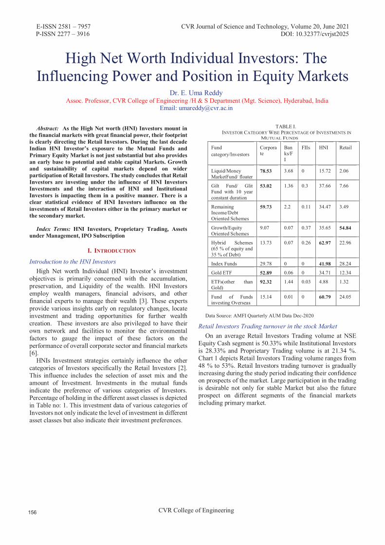
E-ISSN 2581 – 7957 CVR Journal of Science and Technology, Volume 20, June 2021 P-ISSN 2277 – 3916 DOI: 10.32377/cvrjst2025
CVR College of Engineering
High Net Worth Individual Investors: The
Dr. E. Uma Reddy Assoc. Professor, CVR College of Engineering /H & S Department (Mgt. Science), Hyderabad, India
Email: [email protected]
TABLE I. INVESTOR CATEGORY WISE PERCENTAGE OF INVESTMENTS IN
MUTUAL FUNDS
Abstract: As the High Net worth (HNI) Investors mount in the financial markets with great financial power, their footprint is clearly directing the Retail Investors. During the last decade Indian HNI Investor’s exposure to the Mutual Funds and Primary Equity Market is not just substantial but also provides an early base to potential and stable capital Markets. Growth and sustainability of capital markets depend on wider participation of Retail Investors. The study concludes that Retail Investors are investing under the influence of HNI Investors Investments and the interaction of HNI and Institutional Investors is impacting them in a positive manner. There is a clear statistical evidence of HNI Investors influence on the investments of Retail Investors either in the primary market or the secondary market.
Index Terms: HNI Investors, Proprietary Trading, Assets under Management, IPO Subscription
I. INTRODUCTION
Introduction to the HNI Investors High Net worth Individual (HNI) Investor’s investment
objectives is primarily concerned with the accumulation, preservation, and Liquidity of the wealth. HNI Investors employ wealth managers, financial advisors, and other financial experts to manage their wealth [3]. These experts provide various insights early on regulatory changes, locate investment and trading opportunities for further wealth creation. These investors are also privileged to have their own network and facilities to monitor the environmental factors to gauge the impact of these factors on the performance of overall corporate sector and financial markets [6].
HNIs Investment strategies certainly influence the other categories of Investors specifically the Retail Investors [2]. This influence includes the selection of asset mix and the amount of Investment. Investments in the mutual funds indicate the preference of various categories of Investors. Percentage of holding in the different asset classes is depicted in Table no: 1. This investment data of various categories of Investors not only indicate the level of investment in different asset classes but also indicate their investment preferences.
Fund category/Investors
Corporate
Banks/FI
FIIs HNI Retail
Liquid/Money MarketFund/ floater
78.53 3.68 0 15.72 2.06
Gilt Fund/ Glit Fund with 10 year constant duration
53.02 1.36 0.3 37.66 7.66
Remaining Income/Debt Oriented Schemes
59.73 2.2 0.11 34.47 3.49
Growth/Equity Oriented Schemes
9.07 0.07 0.37 35.65 54.84
Hybrid Schemes (65 % of equity and 35 % of Debt)
13.73 0.07 0.26 62.97 22.96
Index Funds 29.78 0 0 41.98 28.24
Gold ETF 52.89 0.06 0 34.71 12.34
ETFs(other than Gold)
92.32 1.44 0.03 4.88 1.32
Fund of Funds investing Overseas
15.14 0.01 0 60.79 24.05
Data Source: AMFI Quarterly AUM Data Dec-2020
Retail Investors Trading turnover in the stock Market On an average Retail Investors Trading volume at NSE
Equity Cash segment is 50.33% while Institutional Investors is 28.33% and Proprietary Trading volume is at 21.34 %. Chart 1 depicts Retail Investors Trading volume ranges from 48 % to 53%. Retail Investors trading turnover is gradually increasing during the study period indicating their confidence on prospects of the market. Large participation in the trading is desirable not only for stable Market but also the future prospect on different segments of the financial markets including primary market.
Influencing Power and Position in Equity Markets
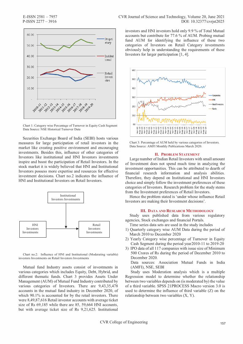
E-ISSN 2581 – 7957 CVR Journal of Science and Technology, Volume 20, June 2021 P-ISSN 2277 – 3916 DOI: 10.32377/cvrjst2025
CVR College of Engineering
Chart 1: Category wise Percentage of Turnover in Equity Cash Segment Data Source: NSE Historical Turnover Data
Securities Exchange Board of India (SEBI) hosts various measures for large participation of retail investors in the market like creating positive environment and encouraging investments. Besides this, influence of other categories of Investors like institutional and HNI Investors investments inspire and boost the participation of Retail Investors. In the stock market it is widely believed that HNI and Institutional Investors possess more expertise and resources for effective investment decisions. Chart no.2 indicates the influence of HNI and Institutional Investors on Retail Investors.
Chart no.2: Influence of HNI and Institutional (Moderating variable)
investors Investments on Retail Investors Investments Mutual fund Industry assets consist of investments in
various categories which includes Equity, Debt, Hybrid, and different thematic funds. Chart 3 provides Assets Under Management (AUM) of Mutual Fund Industry contributed by various categories of Investors. There are 9,43,35,478 accounts in the mutual fund industry in December 2020, of which 90.1% is accounted for by the retail investors. There were 8,49,87,616 Retail investor accounts with average ticket size of Rs 69,185 while there are 85, 59,664 HNI accounts, but with average ticket size of Rs 9,21,625. Institutional
investors and HNI investors hold only 9.9 % of Total Mutual accounts but contribute for 77.6 % of AUM. Probing mutual fund AUM for identifying the influence of these two categories of Investors on Retail Category investments obviously help in understanding the requirements of these Investors for larger participation [1, 4].
Chart 3: Percentage of AUM held by various categories of Investors. Data Source: AMFI Monthly Publications March 2020.
II. PROBLEM STATEMENT Large number of Indian Retail Investors with small amount
of Investment does not spend much time in analyzing the investment opportunities. This can be attributed to dearth of financial research information and analysis abilities. Therefore, they depend on Institutional and HNI Investors choice and simply follow the investment preferences of these categories of Investors. Research problem for the study stems from the Investment preferences of Retail Investors.
Hence the problem stated is ‘under whose influence Retail Investors are making their Investment decisions’.
III. DATA AND RESEARCH METHODOLOGY
Study uses published data from various regulatory agencies, Stock exchanges and financial Portals.
Time series data sets are used in the study includes 1) Quarterly category wise AUM Data during the period of
March 2010 to December 2020 2) Yearly Category wise percentage of Turnover in Equity
Cash Segment during the period year2010-11 to 2019-20 3) IPO data of all 117 companies with issue size of Minimum
500 Crores of Rs during the period of December 2010 to December 2020.
Data sources: Association Mutual Funds in India (AMFI), NSE, SEBI
Study uses Moderation analysis which is a multiple Regression model to determine whether the relationship between two variables depends on (is moderated by) the value of a third variable. SPSS 21PROCESS Macro version 3.0 is used to determine the influence of third variable (Z) on the relationship between two variables (X, Y).
HNI Investors Investments
Retail Investors
Investments
Institutional Investors Investments
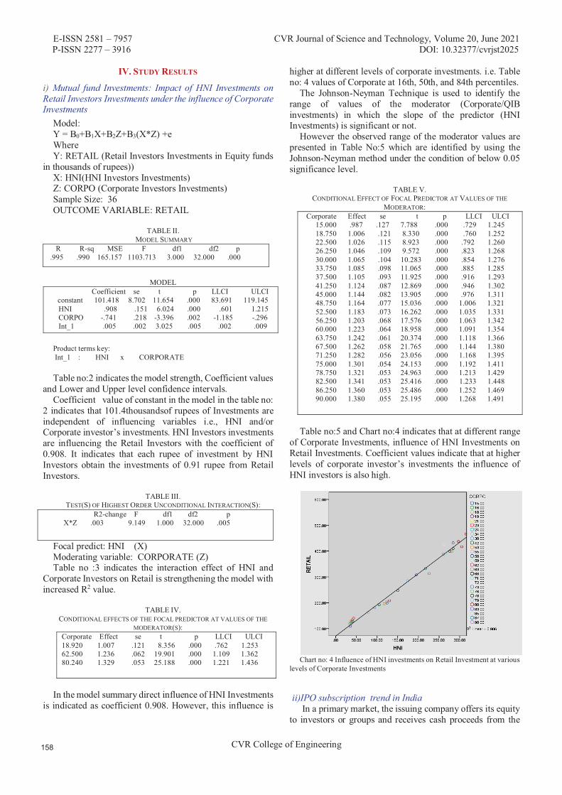
E-ISSN 2581 – 7957 CVR Journal of Science and Technology, Volume 20, June 2021 P-ISSN 2277 – 3916 DOI: 10.32377/cvrjst2025
CVR College of Engineering
IV. STUDY RESULTS
i) Mutual fund Investments: Impact of HNI Investments on Retail Investors Investments under the influence of Corporate Investments
Model: Y = B0+B1X+B2Z+B3(X*Z) +e Where Y: RETAIL (Retail Investors Investments in Equity funds
in thousands of rupees)) X: HNI(HNI Investors Investments) Z: CORPO (Corporate Investors Investments) Sample Size: 36 OUTCOME VARIABLE: RETAIL
TABLE II. MODEL SUMMARY
R R-sq MSE F df1 df2 p .995 .990 165.157 1103.713 3.000 32.000 .000
MODEL
Coefficient se t p LLCI ULCI constant 101.418 8.702 11.654 .000 83.691 119.145
HNI .908 .151 6.024 .000 .601 1.215 CORPO -.741 .218 -3.396 .002 -1.185 -.296 Int_1 .005 .002 3.025 .005 .002 .009
Product terms key: Int_1 : HNI x CORPORATE Table no:2 indicates the model strength, Coefficient values
and Lower and Upper level confidence intervals. Coefficient value of constant in the model in the table no:
2 indicates that 101.4thousandsof rupees of Investments are independent of influencing variables i.e., HNI and/or Corporate investor’s investments. HNI Investors investments are influencing the Retail Investors with the coefficient of 0.908. It indicates that each rupee of investment by HNI Investors obtain the investments of 0.91 rupee from Retail Investors.
TABLE III.
TEST(S) OF HIGHEST ORDER UNCONDITIONAL INTERACTION(S): R2-change F df1 df2 p X*Z .003 9.149 1.000 32.000 .005
Focal predict: HNI (X) Moderating variable: CORPORATE (Z) Table no :3 indicates the interaction effect of HNI and
Corporate Investors on Retail is strengthening the model with increased R2 value.
TABLE IV.
CONDITIONAL EFFECTS OF THE FOCAL PREDICTOR AT VALUES OF THE MODERATOR(S):
Corporate Effect se t p LLCI ULCI 18.920 1.007 .121 8.356 .000 .762 1.253 62.500 1.236 .062 19.901 .000 1.109 1.362 80.240 1.329 .053 25.188 .000 1.221 1.436
In the model summary direct influence of HNI Investments
is indicated as coefficient 0.908. However, this influence is
higher at different levels of corporate investments. i.e. Table no: 4 values of Corporate at 16th, 50th, and 84th percentiles.
The Johnson-Neyman Technique is used to identify the range of values of the moderator (Corporate/QIB investments) in which the slope of the predictor (HNI Investments) is significant or not.
However the observed range of the moderator values are presented in Table No:5 which are identified by using the Johnson-Neyman method under the condition of below 0.05 significance level.
TABLE V.
CONDITIONAL EFFECT OF FOCAL PREDICTOR AT VALUES OF THE MODERATOR:
Corporate Effect se t p LLCI ULCI 15.000 .987 .127 7.788 .000 .729 1.245 18.750 1.006 .121 8.330 .000 .760 1.252 22.500 1.026 .115 8.923 .000 .792 1.260 26.250 1.046 .109 9.572 .000 .823 1.268 30.000 1.065 .104 10.283 .000 .854 1.276 33.750 1.085 .098 11.065 .000 .885 1.285 37.500 1.105 .093 11.925 .000 .916 1.293 41.250 1.124 .087 12.869 .000 .946 1.302 45.000 1.144 .082 13.905 .000 .976 1.311 48.750 1.164 .077 15.036 .000 1.006 1.321 52.500 1.183 .073 16.262 .000 1.035 1.331 56.250 1.203 .068 17.576 .000 1.063 1.342 60.000 1.223 .064 18.958 .000 1.091 1.354 63.750 1.242 .061 20.374 .000 1.118 1.366 67.500 1.262 .058 21.765 .000 1.144 1.380 71.250 1.282 .056 23.056 .000 1.168 1.395 75.000 1.301 .054 24.153 .000 1.192 1.411 78.750 1.321 .053 24.963 .000 1.213 1.429 82.500 1.341 .053 25.416 .000 1.233 1.448 86.250 1.360 .053 25.486 .000 1.252 1.469 90.000 1.380 .055 25.195 .000 1.268 1.491
Table no:5 and Chart no:4 indicates that at different range
of Corporate Investments, influence of HNI Investments on Retail Investments. Coefficient values indicate that at higher levels of corporate investor’s investments the influence of HNI investors is also high.
Chart no: 4 Influence of HNI investments on Retail Investment at various
levels of Corporate Investments
ii)IPO subscription trend in India In a primary market, the issuing company offers its equity
to investors or groups and receives cash proceeds from the
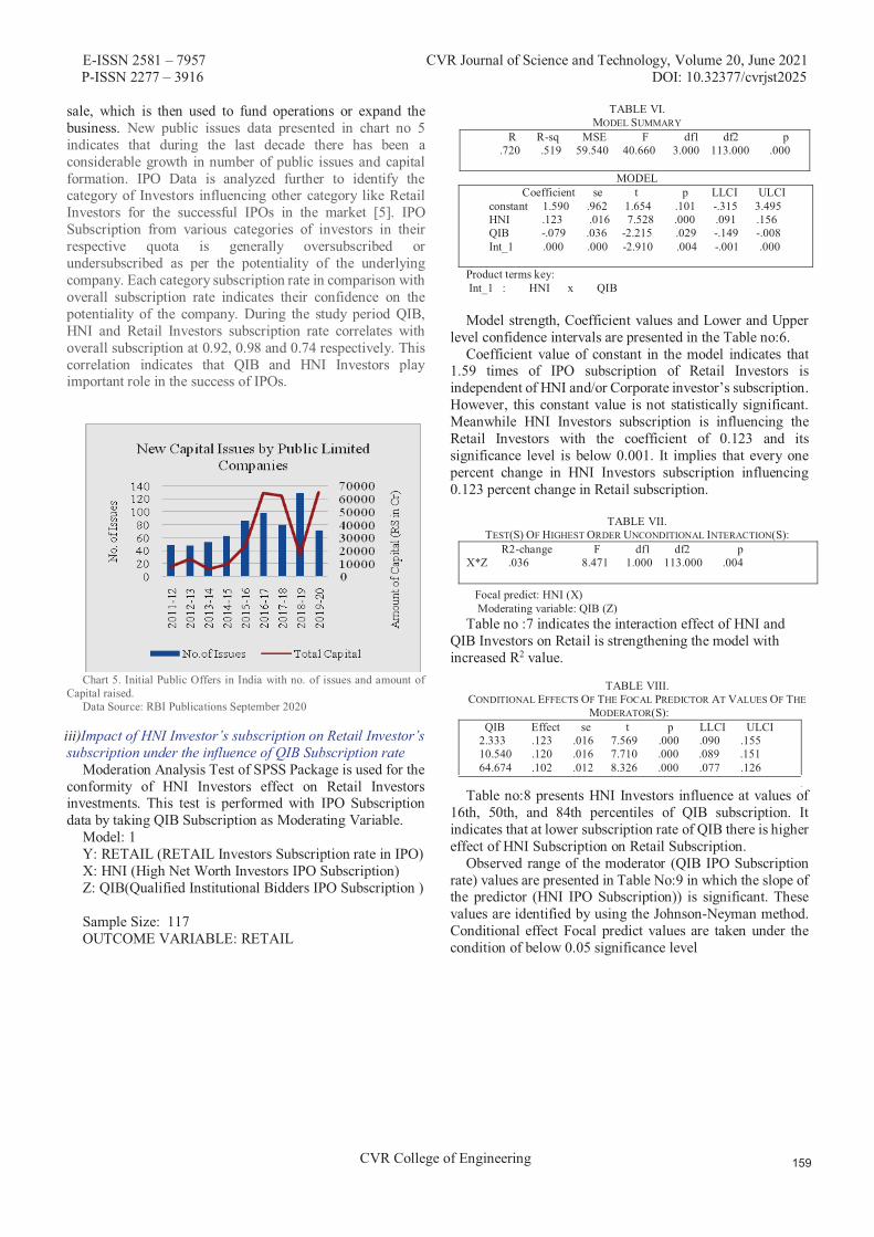
E-ISSN 2581 – 7957 CVR Journal of Science and Technology, Volume 20, June 2021 P-ISSN 2277 – 3916 DOI: 10.32377/cvrjst2025
CVR College of Engineering
sale, which is then used to fund operations or expand the business. New public issues data presented in chart no 5 indicates that during the last decade there has been a considerable growth in number of public issues and capital formation. IPO Data is analyzed further to identify the category of Investors influencing other category like Retail Investors for the successful IPOs in the market [5]. IPO Subscription from various categories of investors in their respective quota is generally oversubscribed or undersubscribed as per the potentiality of the underlying company. Each category subscription rate in comparison with overall subscription rate indicates their confidence on the potentiality of the company. During the study period QIB, HNI and Retail Investors subscription rate correlates with overall subscription at 0.92, 0.98 and 0.74 respectively. This correlation indicates that QIB and HNI Investors play important role in the success of IPOs.
Chart 5. Initial Public Offers in India with no. of issues and amount of Capital raised.
Data Source: RBI Publications September 2020
iii)Impact of HNI Investor’s subscription on Retail Investor’s subscription under the influence of QIB Subscription rate
Moderation Analysis Test of SPSS Package is used for the conformity of HNI Investors effect on Retail Investors investments. This test is performed with IPO Subscription data by taking QIB Subscription as Moderating Variable.
Model: 1 Y: RETAIL (RETAIL Investors Subscription rate in IPO) X: HNI (High Net Worth Investors IPO Subscription) Z: QIB(Qualified Institutional Bidders IPO Subscription )
Sample Size: 117 OUTCOME VARIABLE: RETAIL
TABLE VI. MODEL SUMMARY
R R-sq MSE F df1 df2 p .720 .519 59.540 40.660 3.000 113.000 .000
MODEL Coefficient se t p LLCI ULCI
constant 1.590 .962 1.654 .101 -.315 3.495 HNI .123 .016 7.528 .000 .091 .156 QIB -.079 .036 -2.215 .029 -.149 -.008 Int_1 .000 .000 -2.910 .004 -.001 .000
Product terms key: Int_1 : HNI x QIB
Model strength, Coefficient values and Lower and Upper level confidence intervals are presented in the Table no:6.
Coefficient value of constant in the model indicates that 1.59 times of IPO subscription of Retail Investors is independent of HNI and/or Corporate investor’s subscription. However, this constant value is not statistically significant. Meanwhile HNI Investors subscription is influencing the Retail Investors with the coefficient of 0.123 and its significance level is below 0.001. It implies that every one percent change in HNI Investors subscription influencing 0.123 percent change in Retail subscription.
TABLE VII. TEST(S) OF HIGHEST ORDER UNCONDITIONAL INTERACTION(S):
R2-change F df1 df2 p X*Z .036 8.471 1.000 113.000 .004
Focal predict: HNI (X) Moderating variable: QIB (Z) Table no :7 indicates the interaction effect of HNI and
QIB Investors on Retail is strengthening the model with increased R2 value.
TABLE VIII. CONDITIONAL EFFECTS OF THE FOCAL PREDICTOR AT VALUES OF THE
MODERATOR(S): QIB Effect se t p LLCI ULCI 2.333 .123 .016 7.569 .000 .090 .155 10.540 .120 .016 7.710 .000 .089 .151 64.674 .102 .012 8.326 .000 .077 .126
Table no:8 presents HNI Investors influence at values of 16th, 50th, and 84th percentiles of QIB subscription. It indicates that at lower subscription rate of QIB there is higher effect of HNI Subscription on Retail Subscription.
Observed range of the moderator (QIB IPO Subscription rate) values are presented in Table No:9 in which the slope of the predictor (HNI IPO Subscription)) is significant. These values are identified by using the Johnson-Neyman method. Conditional effect Focal predict values are taken under the condition of below 0.05 significance level

E-ISSN 2581 – 7957 CVR Journal of Science and Technology, Volume 20, June 2021 P-ISSN 2277 – 3916 DOI: 10.32377/cvrjst2025
CVR College of Engineering
TABLE IX. CONDITIONAL EFFECT OF FOCAL PREDICTOR AT VALUES OF THE
MODERATOR
Moderation effect in the table no:9 and Chart no:6 indicates that at higher levels of QIB investor’s subscription the influence of HNI investors is decreasing. However, HNI Investors influence is higher at lower subscription rate of QIB Investors.
Moderation effect which is significant at 0.01level graphically presented in the Chart no 6:
Chart no:6 Influence of HNIs IPO subscription rate on Retail subscription at various levels of QIBs IPO subscription.
Statistical evidence in the model summary and at different subscription rates of QIB Investors indicates that HNI Investors are playing important role in encouraging the Retail Investors at the time of low subscription from QIB Investors and rescuing the companies from under subscription or IPO failures.
V. CONCLUSIONS High Net worth Individual Investors primary objective is
always protection and maximization of their wealth through effective Investments. Investments data of HNIs in the primary and secondary markets of capital market clearly indicate their confidence on the potentiality of the Markets. HNI Investors selection of Assets and level of exposure to a particular investment avenue is clearly paving the way for the followers. HNI Investors subscription rate in IPOs is anchoring the successful capital formation for the business organizations and this matured primary market is essential for the growth of the economy and creating employment.
REFERENCES: [1]. C. P. Chandrasekhar, Sarat Malik and Akriti The elusive retail
investor: How deep can (and should) India’s stock markets be?*The Securities and Exchange Board of India ,Development Research Group.PR No. 43/2016
[2]. Galstyan, A. (2021). Hnwis Investments: Trends And The Capacity To Attract (Visegrad Region Case Study). The Euraseans: Journal On Global Socio-Economic Dynamics, (1(26), 07-18.
[3]. Matt Christensen High Net Worth Individuals and Sustainable Investment - Part I Journal: Australian Journal of Financial PlanningISSN:1833-1106 Volume:4Issue:2 PP 19-25
[4]. Sharma, Kapil Mutual Fund Purchases by High Net Worth Individuals in India.Journal of Management Research (09725814) . Aug2006, Vol. 6 Issue 2, p59-71. 13p.
[5]. Thomas J. Chemmanur, Gang Hu, Jiekun Huang The Role of Institutional Investors in Initial Public Offerings The Review of Financial Studies, Volume 23, Issue 12, December 2010, PP 4496–4540,
[6]. “World Wealth Report 2020" Capgemini. Archived (PDF) from the original on 2020-11-10. Retrieved 2020-11-09. https://www.capgemini.com/news/research-world-wealth-report-2020.
QIB Effect se t p LLCI ULCI .260 .123 .016 7.532 .000 .091 .156
9.860 .120 .016 7.699 .000 .089 .151 19.460 .117 .015 7.860 .000 .087 .146 29.060 .114 .014 8.010 .000 .085 .142 38.660 .110 .014 8.142 .000 .084 .137 48.260 .107 .013 8.245 .000 .081 .133 57.860 .104 .013 8.310 .000 .079 .129 67.460 .101 .012 8.324 .000 .077 .125 77.060 .098 .012 8.275 .000 .074 .121 86.660 094 .012 8.154 .000 .071 .117 96.260 .091 .011 7.957 .000 .068 .114 105.860 .088 .011 7.685 .000 .065 .111 115.460 .085 .012 7.343 .000 .062 .108 125.060 .081 .012 6.946 .000 .058 .105 134.660 .078 .012 6.507 .000 .054 .102 144.260 .075 .012 6.046 .000 .050 .100 153.860 .072 .013 5.576 .000 .046 .097 163.460 .069 .013 5.110 .000 .042 .095 173.060 .065 .014 4.659 .000 .038 .093 182.660 .062 .015 4.229 .000 .033 .091 192.260 .059 .015 3.824 .000 .028 .090

1. M. Ashok Kumar, Batchu RamanjaneyuluEffect of Egg Shell Powder on Index and EngineeringProperties of Clayey Soil
2. A High-Performance FIR Filter Architecture usingSymmetry and Distributed Arithmetic Logic
Venkata Krishna Odugu, Janardhana RaoBitra, Satish Bojjawar
3. A Survey on Leaf Disease Detection Techniques A.S Neelima, C.V.S. Sathyamurthy
4. K.L.N. Murthy, Darbha Rohit,A.C. Uma Maheshwar Rao
Impact of Post Welding Heat Treatment Process onMicrostructure and Mechanical Properties of TigWelded Ss-304 & Ss316l Dissimilar Metals
5. Effect of Water Level on Mechanical Properties ofUnderwater Friction Stir Welded Aluminum Alloys
G. Mrudula, Sk. Mohammad Shareef,P. Bhargavi
6. Design and Fabrication of Seabin Project for EfficientCollection of Water Waste using Solar Energy
Sarat Kumar Sahoo, S. T. Ahmed Nizami,Shaik Wahajuddin, Gampa Smruthi
7. Raghavendra Kulkarni1, K. GuruvidyathriExploration of Multicomponent Phase Diagrams andEvaluation of Calphad Databases

E-ISSN 2581 –7957 CVR Journal of Science and Technology, Volume 20, June 2021 P-ISSN 2277 – 3916 DOI: 10.32377/cvrjstxxxx
CVR College of Engineering
Template for the Preparation of Papers for Publication in CVR Journal of Science and
TechnologyFirst Dr. A. Author1 and Second B. Author2
1Designation, Name of Institution/Department, City, CountryEmail: [email protected]
2Designation, Name of Institution/Department, City, CountryEmail: [email protected]
Abstract: These instructions give you basic guidelines for preparing camera-ready papers for CVR College journal Publications. Your cooperation in this matter will help in producing a high-quality journal.
Index Terms: first term, second term, third term, fourth term, fifth term, sixth term
I. INTRODUCTION
Your goal is to simulate the usual appearance of papers in a Journal Publication of the CVR College. We are requesting that you follow these guidelines as closely as possible. It should be original work. Format must be done as per the template specified. Diagrams with good clarity withrelevant reference within the text are to be given. References are to be cited within the body of the paper. Number of pages must not be less than five with minimum number of 4000 words and not exceeding eight pages. The journal is published in colour. Colours used for headings, subheadings and other captions must be strictly as per the template given in colour.
A. Full-Sized Camera-Ready (CR) CopyPrepare your CR paper in full-size format, on A4 paper
(210 x 297 mm or 8.27 x 11.69 in). No header or footer, no page number.
Type sizes and typefaces: Follow the type sizes specified in Table I. As an aid in gauging type size, 1 point is about 0.35 mm. The size of the lowercase letter “j” will give the point size. Times New Roman has to be the font for main text. Paper should be single spaced.
Margins: Top and Bottom = 24.9mm (0.98 in), Left and Right = 16 mm (0.63 in). The column width is 86mm (3.39in). The space between the two columns is 6mm (0.24 in). Paragraph indentation is 3.7 mm (0.15 in).
Left- and right-justify your columns. Use tables and figures to adjust column length. On the last page of your paper, adjust the lengths of the columns so that they are equal. Use automatic hyphenation and check spelling. Digitize or paste down figures.
For the Title use 24-point Times New Roman font, an initial capital letter for each word. Its paragraph description should be set so that the line spacing is single with 6-point spacing before and 6-point spacing after. Use two additional line spacings of 10 points before the beginning of the double column section, as shown above.
Each major section begins with a Heading in 10 point Times New Roman font centered within the column and numbered using Roman numerals (except for REFERENCES), followed by a period, two spaces, and the title using an initial capital letter for each word. The remaining letters are in SMALL CAPITALS (8 point). The paragraph description of the section heading line should be set for 12 points beforeand 6 points after.
Subheadings should be 10 point, italic, left justified, and numbered with letters (A, B, …), followed by a period, twospaces, and the title using an initial capital letter for each word. The paragraph description of the subheading line should be set for 6 points before and 3 points after.
For main text, paragraph spacing should be single spaced, no space between paragraphs. Paragraph indentation should be 3.7mm/0.21in, but no indentation for abstract & index terms.
II. HELPFUL HINTS
A. Figures And TablesPosition figures and tables at the tops and bottoms of
columns. Avoid placing them in the middle of columns. Large figures and tables may span across both columns. Leave sufficient room between the figures/tables and the main text. Figure captions should be centered below the figures; table captions should be centered above. Avoid placing figures and tables before their first mention in the
TABLE I. TYPE SIZES FOR CAMERA-READY PAPERS
Type size
(pts.)
Appearance
Regular Bold Italic
6 Table caption, table superscripts
8
Tables, table names, f irst letters in table captions, figure captions, footnotes, text subscripts, and superscripts
9 References, authors’ biographies
Abstract
10Section titles ,Authors’
affiliations, main text, equations, first letters in section titles
Subheading
11 Authors’ names
24 Paper title
E-ISSN 2581 –7957 CVR Journal of Science and Technology, Volume 20, June 2021 P-ISSN 2277 – 3916 DOI: 10.32377/cvrjstxxxx
CVR College of Engineering
Figure 2. Note how the caption is centered in the column.
text. Use the abbreviation “Fig. 1,” even at the beginning of a sentence.
To figure axis labels, use words rather than symbols. Do not label axes only with units. Do not label axes with a ratio
of quantities and units. Figure labels should be legible, about 8-point type.
All figures, tables and references must be cited in the text.Please indicate the broad area/specializations into which
the research paper falls, in the covering letter/mail to the Editor, so that reviewers with those specializations may be identified.
B. ReferencesNumber citations consecutively in square brackets [1].
Punctuation follows the bracket [2]. Use “Ref. [3]” or “Reference [3]” at the beginning of a sentence:
Give all authors’ names; use “et al.” if there are six authors or more. Papers that have not been published, even if they have been submitted for publication, should be cited as “unpublished” [4]. Papers that have been accepted for publication should be cited as “in press” [5]. In a paper title, capitalize the first word and all other words except for conjunctions, prepositions less than seven letters, and prepositional phrases. Good number of references must be given.
Latest references in the area must be included and every refence must be cited in the text of the research article.
C. FootnotesNumber footnotes separately in superscripts 1, 2, …. Place
the actual footnote at the bottom of the column in which it was cited, as in this column. See first page footnote as an example.
D. Abbreviations and AcronymsDefine abbreviations and acronyms the first time they are
used in the text, even after they have been defined in the
abstract. Do not use abbreviations in the title unless they are unavoidable.
E. EquationsEquations should be left justified in the column. The
paragraph description of the line containing the equation should be set for 6 points before and 6 points after. Number equations consecutively with equation numbers in parentheses flush with the right margin, as in (1). Italicize Roman symbols for quantities and variables, but not Greek symbols. Punctuate equations with commas or periods when they are part of a sentence, as in
cba =+ . (1)
Symbols in your equation should be defined before the equation appears or immediately following. Use “(1),” not “Eq. (1)” or “equation (1),” except at the beginning of a sentence: “Equation (1) is ...”
F. Other RecommendationsUse either SI (MKS) or CGS as primary units. (SI units
are encouraged.) If your native language is not English, try to get a native English-speaking colleague to proofread your paper. Do not add page numbers.
III. CONCLUSIONS
The authors can conclude on the topic discussed and proposed, future enhancement of research work can also be briefed here.
REFERENCES
[1] G. Eason, B. Noble, and I. N. Sneddon, “On certain integrals of Lipschitz-Hankel type involving products of Bessel functions,” Phil. Trans. Roy. Soc. London, vol. A247, pp. 529–551, April 1955.
[2] J. Clerk Maxwell, A Treatise on Electricity and Magnetism, 3rd ed., vol. 2. Oxford: Clarendon, 1892, pp.68–73.
[3] I. S. Jacobs and C. P. Bean, “Fine particles, thin films and exchange anisotropy,” in Magnetism, vol. III, G. T. Rado and H. Suhl, Eds. New York: Academic, 1963, pp. 271–350.
[4] K. Elissa, “Title of paper if known,” unpublished.[5] R. Nicole, “Title of paper with only first word capitalized”, J.
Name Stand. Abbrev., in press.[6] Y. Yorozu, M. Hirano, K. Oka, and Y. Tagawa, “Electron
spectroscopy studies on magneto-optical media and plastic substrate interface,” IEEE Transl. J. Magn. Japan, vol. 2, pp. 740–741, August 1987 [Digests 9th Annual Conf. Magnetics Japan, p. 301, 1982].
[7] M. Young, The Technical Writer's Handbook. Mill Valley, CA: University Science, 1989.
[8] T. Ali, B.K. Subhash and R.C. Biradar, “A Miniaturized Decagonal Sierpinski UWB Fractal Antenna”, PIERS C, vol. 84, pp. 161-174, 2018.