vocabulary lists in computational historical linguistics

ii

“mylic_thesis” — 2013/12/19 — 20:14 — page 1 — #1 ii

ii

ii

Taraka Rama

Vocabulary lists in computationalhistorical linguistics

ii


ii

ii

Data linguistica<http://www.svenska.gu.se/publikationer/data-linguistica/>

Editor: Lars Borin

SpråkbankenDepartment of SwedishUniversity of Gothenburg

25 • 2014

ii


ii

ii

Taraka Rama

Vocabulary lists incomputational historicallinguistics

Gothenburg 2014

ii


ii

ii

Data linguistica 25ISBN 978-91-87850-52-3ISSN 0347-948X

Printed in Sweden byReprocentralen, Campusservice Lorensberg, University of Gothenburg2014

Typeset in LATEX 2ε by the author

Cover design by Kjell Edgren, Informat.se

Front cover illustration:A network representation of relations between Dravidian languages.by Rama and Kolachina (2013) c©

Author photo on back cover by Kristina Holmlid

ii

“mylic_thesis” — 2013/12/19 — 20:14 — page i — #5 ii

ii

ii

ABSTRACT

Computational analysis of historical and typological data has made great progr-ess in the last fifteen years. In this thesis, we work with vocabulary lists foraddressing some classical problems in historical linguistics such as discrimi-nating related languages from unrelated languages, assigning possible dates tosplits in a language family, employing structural similarity for language classi-fication, and providing an internal structure to a language family. In this thesis,we compare the internal structure inferred from vocabulary lists to the familytree structure inferred through the comparative method. We also explore theranking of lexical items in the widely used Swadesh word list and compare ourranking to another quantitative reranking method and short lists composed fordiscovering long-distance genetic relationships. We also show that the choiceof string similarity measures is important for internal classification and for dis-criminating related from unrelated languages. The dating system presented inthis thesis can be used for assigning age estimates to any new language groupand overcomes the criticism of constant rate of lexical change assumed byglottochronology. An important conclusion from these results is that n-gramapproaches can be used for different historical linguistic purposes. The fieldis undergoing a shift from – the application of computational methods to –short, hand-crafted vocabulary lists to automatically extracted word lists fromcorpora. Thus, we also experiment with parallel corpora for automatically ex-tracting cognates to infer a family tree from the cognates.

ii

“mylic_thesis” — 2013/12/19 — 20:14 — page ii — #6 ii

ii

ii

ii

“mylic_thesis” — 2013/12/19 — 20:14 — page iii — #7 ii

ii

ii

SAMMANFATTNING

Datorbaserad analys av historiska data har gjort stora framsteg under det sen-aste decenniet. I denna licentiatuppsats använder vi ordlistor för att ta oss annågra klassiska problem inom historisk lingvistik. Exempel på sådana problemär hur man avgör vilka språk som är släkt med varandra och vilka som inteär det, hur man tidsbestämmer rekonstruerade urspråk, hur man klassificerarspråk på grundval av strukturella likheter och skillnader, samt hur man slutersig till den interna strukturen i en språkfamilj (dess ‘familjeträd’).

I uppsatsen jämför vi metoder som använts för att postulera språkliga fa-miljeträd. Specifikt jämför vi ordlistebaserade metoder med den traditionellakomparativa metoden, som även använder andra språkliga drag för jämförelsen.Med fokus på ordlistor jämför vi den ofta använda Swadesh-listan med al-ternativa listor föreslagna i litteraturen eller framtagna i vår egen forskning,med avseende på deras användbarhet för att angripa de nämnda historisk-lingvistiska problemen.

Vi visar också i experiment att valet av likhetsmått är mycket betydelsefulltnär strängjämförelser används för att bestämma den interna strukturen i enspråkfamilj eller för att skilja besläktade och obesläktade språk åt. Ett viktigtresultat av dessa experiment är att n-grambaserade metoder lämpar sig mycketväl för flera olika språkhistoriska ändamål.

De metoder för språklig datering som presenteras här kan användas för atttidsbestämma nya språkfamiljer, dock utan att vara beroende av antagandet attförändringen av ett språks basordförråd är konstant över tid, ett hårt kritiseratantagande som ligger till grund för glottokronologin som den ursprungligenformulerades.

Metodologiskt har man inom området nu börjat utforska möjligheten attövergå från att arbeta med korta, på förhand givna ordlistor till att tillämpaspråkteknologiska metoder på stora språkliga material, t ex hela (traditionella)lexikon eller strukturerat språkligt material som extraheras ur flerspråkiga kor-pusar. I uppsatsen utforskas användningen av parallella korpusar för att auto-matiskt finna ord med ett gemensamt ursprung (kognater) och därefter härledaett språkligt familjeträd från kognatlistorna.

ii

“mylic_thesis” — 2013/12/19 — 20:14 — page iv — #8 ii

ii

ii

ii

“mylic_thesis” — 2013/12/19 — 20:14 — page vi — #10 ii

ii

ii

ii

“mylic_thesis” — 2013/12/19 — 20:14 — page vii — #11 ii

ii

ii

CONTENTS

Abstract i

Sammanfattning iii

Acknowledgements v

I Introduction to the thesis 1

1 Introduction 31.1 Computational historical linguistics . . . . . . . . . . . . . . . . 3

1.1.1 Historical linguistics . . . . . . . . . . . . . . . . . . . 41.1.2 What is computational historical linguistics? . . . . . . . 4

1.2 Questions, answers, and contributions . . . . . . . . . . . . . . . 91.3 Overview of the thesis . . . . . . . . . . . . . . . . . . . . . . . 11

2 Computational historical linguistics 152.1 Differences and diversity . . . . . . . . . . . . . . . . . . . . . . 152.2 Language change . . . . . . . . . . . . . . . . . . . . . . . . . . 19

2.2.1 Sound change . . . . . . . . . . . . . . . . . . . . . . . 192.2.2 Semantic change . . . . . . . . . . . . . . . . . . . . . 27

2.3 How do historical linguists classify languages? . . . . . . . . . . 312.3.1 Ingredients in language classification . . . . . . . . . . . 312.3.2 The comparative method and reconstruction . . . . . . . 34

2.4 Alternative techniques in language classification . . . . . . . . . 442.4.1 Lexicostatistics . . . . . . . . . . . . . . . . . . . . . . 442.4.2 Beyond lexicostatistics . . . . . . . . . . . . . . . . . . 45

2.5 A language classification system . . . . . . . . . . . . . . . . . . 472.6 Tree evaluation . . . . . . . . . . . . . . . . . . . . . . . . . . . 47

2.6.1 Tree comparison measures . . . . . . . . . . . . . . . . 482.6.2 Beyond trees . . . . . . . . . . . . . . . . . . . . . . . . 49

2.7 Dating and long-distance relationship . . . . . . . . . . . . . . . 502.7.1 Non-quantitative methods in linguistic paleontology . . . 52

2.8 Conclusion . . . . . . . . . . . . . . . . . . . . . . . . . . . . . 54

ii

“mylic_thesis” — 2013/12/19 — 20:14 — page viii — #12 ii

ii

ii

viii Contents

3 Databases 553.1 Cognate databases . . . . . . . . . . . . . . . . . . . . . . . . . 55

3.1.1 Dyen’s Indo-European database . . . . . . . . . . . . . 563.1.2 Ancient Indo-European database . . . . . . . . . . . . . 563.1.3 Intercontinental Dictionary Series (IDS) . . . . . . . . . 563.1.4 World loanword database . . . . . . . . . . . . . . . . . 573.1.5 List’s database . . . . . . . . . . . . . . . . . . . . . . . 573.1.6 Austronesian Basic Vocabulary Database (ABVD) . . . . 58

3.2 Typological databases . . . . . . . . . . . . . . . . . . . . . . . 583.2.1 Syntactic Structures of the World’s Languages . . . . . . 583.2.2 Jazyki Mira . . . . . . . . . . . . . . . . . . . . . . . . 583.2.3 AUTOTYP . . . . . . . . . . . . . . . . . . . . . . . . 58

3.3 Other comparative linguistic databases . . . . . . . . . . . . . . . 593.3.1 ODIN . . . . . . . . . . . . . . . . . . . . . . . . . . . 593.3.2 PHOIBLE . . . . . . . . . . . . . . . . . . . . . . . . . 593.3.3 World phonotactic database . . . . . . . . . . . . . . . . 593.3.4 WOLEX . . . . . . . . . . . . . . . . . . . . . . . . . . 59

3.4 Conclusion . . . . . . . . . . . . . . . . . . . . . . . . . . . . . 60

4 Summary and future work 614.1 Summary . . . . . . . . . . . . . . . . . . . . . . . . . . . . . . 614.2 Future work . . . . . . . . . . . . . . . . . . . . . . . . . . . . . 62

II Papers on application of computational techniques to vo-cabulary lists for automatic language classification 65

5 Estimating language relationships from a parallel corpus 675.1 Introduction . . . . . . . . . . . . . . . . . . . . . . . . . . . . . 675.2 Related work . . . . . . . . . . . . . . . . . . . . . . . . . . . . 695.3 Our approach . . . . . . . . . . . . . . . . . . . . . . . . . . . . 705.4 Dataset . . . . . . . . . . . . . . . . . . . . . . . . . . . . . . . 715.5 Experiments . . . . . . . . . . . . . . . . . . . . . . . . . . . . 735.6 Results and discussion . . . . . . . . . . . . . . . . . . . . . . . 745.7 Conclusions and future work . . . . . . . . . . . . . . . . . . . . 76

6 N-gram approaches to the historical dynamics of basic vocabu-lary 79

6.1 Introduction . . . . . . . . . . . . . . . . . . . . . . . . . . . . . 796.2 Background and related work . . . . . . . . . . . . . . . . . . . 82

6.2.1 Item stability and Swadesh list design . . . . . . . . . . 82

ii

“mylic_thesis” — 2013/12/19 — 20:14 — page ix — #13 ii

ii

ii

Contents ix

6.2.2 The ASJP database . . . . . . . . . . . . . . . . . . . . 836.2.3 Earlier n-gram-based approaches . . . . . . . . . . . . . 84

6.3 Method . . . . . . . . . . . . . . . . . . . . . . . . . . . . . . . 856.4 Results and discussion . . . . . . . . . . . . . . . . . . . . . . . 876.5 Conclusions . . . . . . . . . . . . . . . . . . . . . . . . . . . . . 89

7 Typological distances and language classification 917.1 Introduction . . . . . . . . . . . . . . . . . . . . . . . . . . . . . 917.2 Related Work . . . . . . . . . . . . . . . . . . . . . . . . . . . . 927.3 Contributions . . . . . . . . . . . . . . . . . . . . . . . . . . . . 947.4 Database . . . . . . . . . . . . . . . . . . . . . . . . . . . . . . 94

7.4.1 WALS . . . . . . . . . . . . . . . . . . . . . . . . . . . 947.4.2 ASJP . . . . . . . . . . . . . . . . . . . . . . . . . . . . 957.4.3 Binarization . . . . . . . . . . . . . . . . . . . . . . . . 95

7.5 Measures . . . . . . . . . . . . . . . . . . . . . . . . . . . . . . 967.5.1 Internal classification accuracy . . . . . . . . . . . . . . 967.5.2 Lexical distance . . . . . . . . . . . . . . . . . . . . . . 98

7.6 Results . . . . . . . . . . . . . . . . . . . . . . . . . . . . . . . 997.6.1 Internal classification . . . . . . . . . . . . . . . . . . . 997.6.2 Lexical divergence . . . . . . . . . . . . . . . . . . . . 100

7.7 Conclusion . . . . . . . . . . . . . . . . . . . . . . . . . . . . . 101

8 Phonotactic diversity and time depth of language families 1038.1 Introduction . . . . . . . . . . . . . . . . . . . . . . . . . . . . . 103

8.1.1 Related work . . . . . . . . . . . . . . . . . . . . . . . 1048.2 Materials and Methods . . . . . . . . . . . . . . . . . . . . . . . 106

8.2.1 ASJP Database . . . . . . . . . . . . . . . . . . . . . . 1068.2.2 ASJP calibration procedure . . . . . . . . . . . . . . . . 1068.2.3 Language group size and dates . . . . . . . . . . . . . . 1078.2.4 Calibration procedure . . . . . . . . . . . . . . . . . . . 1098.2.5 N-grams and phonotactic diversity . . . . . . . . . . . . 110

8.3 Results and Discussion . . . . . . . . . . . . . . . . . . . . . . . 1118.3.1 Worldwide date predictions . . . . . . . . . . . . . . . . 117

8.4 Conclusion . . . . . . . . . . . . . . . . . . . . . . . . . . . . . 118

9 Evaluation of similarity measures for automatic language classi-fication. 119

9.1 Introduction . . . . . . . . . . . . . . . . . . . . . . . . . . . . . 1199.2 Related Work . . . . . . . . . . . . . . . . . . . . . . . . . . . . 121

9.2.1 Cognate identification . . . . . . . . . . . . . . . . . . . 1229.2.2 Distributional measures . . . . . . . . . . . . . . . . . . 123

ii

“mylic_thesis” — 2013/12/19 — 20:14 — page x — #14 ii

ii

ii

x Contents

9.3 Contributions . . . . . . . . . . . . . . . . . . . . . . . . . . . . 1249.4 Database and expert classifications . . . . . . . . . . . . . . . . . 125

9.4.1 Database . . . . . . . . . . . . . . . . . . . . . . . . . . 1259.5 Methodology . . . . . . . . . . . . . . . . . . . . . . . . . . . . 127

9.5.1 String similarity . . . . . . . . . . . . . . . . . . . . . . 1279.5.2 N-gram similarity . . . . . . . . . . . . . . . . . . . . . 128

9.6 Evaluation measures . . . . . . . . . . . . . . . . . . . . . . . . 1309.6.1 Dist . . . . . . . . . . . . . . . . . . . . . . . . . . . . 1309.6.2 Correlation with WALS . . . . . . . . . . . . . . . . . . 1319.6.3 Agreement with Ethnologue . . . . . . . . . . . . . . . 131

9.7 Item-item vs. length visualizations . . . . . . . . . . . . . . . . . 1329.8 Results and discussion . . . . . . . . . . . . . . . . . . . . . . . 1349.9 Conclusion . . . . . . . . . . . . . . . . . . . . . . . . . . . . . 136

References 138

Appendices

A Supplementary information to phonotactic diversity 163A.1 Data . . . . . . . . . . . . . . . . . . . . . . . . . . . . . . . . . 163A.2 Diagnostic Plots . . . . . . . . . . . . . . . . . . . . . . . . . . 166A.3 Dates of the world’s languages . . . . . . . . . . . . . . . . . . . 169

B Appendix to evaluation of string similarity measures 179B.1 Results for string similarity . . . . . . . . . . . . . . . . . . . . . 179B.2 Plots for length normalization . . . . . . . . . . . . . . . . . . . 186

ii


ii

ii

Part I

Introduction to the thesis

ii


ii

ii

ii


ii

ii

1 INTRODUCTION

This licentiate thesis can be viewed as an attempt at applying techniques fromLanguage Technology (LT; also known as Natural Language Processing [NLP]or Computational Linguistics [CL]) to the traditional historical linguistics prob-lems such as dating of language families, structural similarity vs genetic simi-larity, and language classification.

There are more than 7,000 languages in this world (Lewis, Simons andFennig 2013) and more than 100,000 unique languoids (Nordhoff and Ham-marström 2012; it is known as Glottolog) where a languoid is defined as aset of documented and closely related linguistic varieties. Modern humans ap-peared on this planet about 100,000–150,000 years ago (Vigilant et al. 1991;Nettle 1999a). Given that all modern humans descended from a small Africanancestral population, did all the 7,000 languages descend from a common lan-guage? Did language emerge from a single source (monogenesis) or from mul-tiple sources at different times (polygenesis)? A less ambitious question wouldbe if there are any relations between these languages? Or do these languagesfall under a single family – descended from a single language which is nolonger spoken – or multiple families? If they fall under multiple families, howare they related to each other? What is the internal structure of a single lan-guage family? How old is a family or how old are the intermediary membersof a family? Can we give reliable age estimates to these languages? This thesisattempts to answer these questions. These questions come under the scientificdiscipline of historical linguistics. More specifically, this thesis operates in thesubfield of computational historical linguistics.

1.1 Computational historical linguistics

This section gives a brief introduction to historical linguistics and then to therelated field of computational historical linguistics.1

1To the best of our knowledge, Lowe and Mazaudon (1994) were the first to use the term.

ii


ii

ii

4 Introduction

1.1.1 Historical linguistics

Historical linguistics is the oldest branch of modern linguistics. Historical lin-guistics is concerned with language change, the processes introducing the lan-guage change and also identifying the (pre-)historic relationships between lan-guages (Trask 2000: 150). This branch works towards identifying the not-so-apparent relations between languages. The branch has succeeded in identifyingthe relation between languages spoken in the Indian sub-continent, the Uyghurregion of China, and Europe; the languages spoken in Madagascar islands andthe remote islands in the Pacific Ocean.

A subbranch of historical linguistics is comparative linguistics. Accordingto Trask (2000: 65), comparative linguistics is a branch of historical linguisticswhich seeks to identify and elucidate genetic relationships among languages.Comparative linguistics works through the comparison of linguistic systems.Comparativists compare vocabulary items (not any but following a few generalguidelines) and morphological forms; and accumulate the evidence for lan-guage change through systematic sound correspondences (and sound shifts) topropose connections between languages descended through modification froma common ancestor.

The work reported in this thesis lies within the area of computational his-torical linguistics which relates to the application of computational techniquesto address the traditional problems in historical linguistics.

1.1.2 What is computational historical linguistics?

The use of mathematical and statistical techniques to classify languages (Kroe-ber and Chrétien 1937) and evaluate the language relatedness hypothesis (Kroe-ber and Chrétien 1939; Ross 1950; Ellegård 1959) has been attempted in thepast. Swadesh (1950) invented the method of lexicostatistics which works withstandardized vocabulary lists but the similarity judgment between the words isbased on cognacy rather than the superficial word form similarity technique ofmultilateral comparison (Greenberg 1993: cf. section 2.4.2). Swadesh (1950)uses cognate counts to posit internal relationships between a subgroup of a lan-guage family. Cognates are related words across languages whose origin canbe traced back to a (reconstructed or documented) word in a common ances-tor. Cognates are words such as Sanskrit dva and Armenian erku ‘two’ whoseorigin can be traced back to a common ancestor. Cognates usually have similarform and also similar meaning and are not borrowings (Hock 1991: 583–584).The cognates were not identified through a computer but by a manual proce-dure beforehand to arrive at the pair-wise cognate counts.

ii


ii

ii

1.1 Computational historical linguistics 5

Hewson 1973 (see Hewson 2010 for a more recent description) can beconsidered the first such study where computers were used to reconstruct thewords of Proto-Algonquian (the common ancestor of Algonquian languagefamily). The dictionaries of four Algonquian languages – Fox, Cree, Ojibwa,and Menominee – were converted into computer-readable format – skeletalforms, only the consonants are fed into the computer and vowels are omitted– and then project an ancestral form (proto-form; represented by a *) for aword form by searching through all possible sound-correspondences. The pro-jected proto-forms for each language are alphabetically sorted to yield a setof putative proto-forms for the four languages. Finally, a linguist with suffi-cient knowledge of the language family would then go through the putativeproto-list and remove the unfeasible cognates.

CHL aims to design computational methods to identify linguistic differ-ences between languages based on different aspects of language: phonology,morphology, lexicon, and syntax. CHL also includes computational simula-tions of language change in speech communities (Nettle 1999b), simulation ofdisintegration (divergence) of proto-languages (De Oliveira, Sousa and Wich-mann 2013), the relation between population sizes and rate of language change(Wichmann and Holman 2009a), and simulation of the current distribution oflanguage families (De Oliveira et al. 2008). Finally, CHL proposes and studiesformal and computational models of linguistic evolution through language ac-quisition (Briscoe 2002), computational and evolutionary aspects of language(Nowak, Komarova and Niyogi 2002; Niyogi 2006).

In practice, historical linguists work with word lists – selected words whichare not nursery forms, onomatopoeic forms, chance similarities, and borrow-ings (Campbell 2003) – for the majority of the time. Dictionaries are a naturalextension to word lists (Wilks, Slator and Guthrie 1996). Assuming that weare provided with bilingual dictionaries of some languages, can we simulatethe task of a historical linguist? How far can we automate the steps of weedingout borrowings, extracting sound correspondences, and positing relationshipsbetween languages? An orthogonal task to language comparison is the task ofthe comparing the earlier forms of an extant language to its modern form.

A related task in comparative linguistics is internal reconstruction. Internalreconstruction seeks to identify the exceptions to patterns present in extantlanguages and then reconstruct the regular patterns in the older stages. Thelaryngeal hypothesis in the Proto-Indo-European (PIE) is a classical case ofinternal reconstruction. Saussure applied internal reconstruction to explain theaberrations in the reconstructed root structures of PIE.

PIE used vowel alternations such as English sing/sang/sung – also knownas ablaut or apophony – for grammatical purposes (Trask 1996: 256). The gen-eral pattern for root structures was CVC with V reconstructed as *e. However

ii


ii

ii

6 Introduction

there were exceptions to the reconstructed root of the forms such as CV- orVC- where V could be *a or *o. Saussure conjectured that there were threeconsonants: h1, h2, h3 in pre-PIE. Imagining each consonant as a functionwhich operates on vowels **e, **a and **o; h1 would render **e > *e; h2renders **e > *a; h3 renders **e > *o.2 Finally, the consonant in pre-vocalicposition affected the vowel quality and in post-vocalic position, it also affectedthe preceding vowel length through compensatory lengthening. This conjec-ture was corroborated through the discovery of the [h

ˇ] consonant in Hittite

texts.The following excerpt from the Lord’s Prayer shows the differences be-

tween Old English (OE) and current-day English (Hock 1991: 2–3):

Fæder ure þu þe eart on heofonum,Si þin nama gehalgod.

‘Father of ours, thou who art in heavens,Be thy name hallowed.’

In the above excerpt, Old English (OE) eart is the ancestor to English art‘are’ which is related to PIE *h1er-. The OE si (related to German sind) andEnglish be are descendants from different PIE roots *h1es- and *bhuh2- butserve the same purpose.

The work reported in this thesis attempts to devise and apply computationaltechniques (developed in LT) to both hand-crafted word lists as well as auto-matically extracted word lists from corpora.

An automatic mapping of the words in digitized text, from the middle ages,to the current forms would be a CHL task. Another task would be to iden-tify the variations in written forms and normalize the orthographic variations.These tasks fall within the field of NLP for historical texts (Piotrowski 2012).For instance, deriving the suppletive verbs such as go, went or adjectives good,better, best from ancestral forms or automatically identifying the correspond-ing cognates in Sanskrit would also be a CHL task.

There has been a renewed interest in the application of computational andquantitative techniques to the problems in historical linguistics for the last fif-teen years. This new wave of publications has been met with initial skepticismwhich lingers from the past of glottochronology.3 However, the initial skep-ticism has given way to consistent work in terms of methods (Agarwal andAdams 2007), workshop(s) (Nerbonne and Hinrichs 2006), journals (Wich-mann and Good 2011), and an edited volume (Borin and Saxena 2013).

2** denotes a pre-form in the proto-language.3See Nichols and Warnow (2008) for a survey on this topic.

ii


ii

ii

1.1 Computational historical linguistics 7

The new wave of CHL publications are co-authored by linguists, computerscientists, computational linguists, physicists and evolutionary biologists. Ex-cept for sporadic efforts (Kay 1964; Sankoff 1969; Klein, Kuppin and Meives1969; Durham and Rogers 1969; Smith 1969; Wang 1969; Dobson et al.1972; Borin 1988; Embleton 1986; Dyen, Kruskal and Black 1992; Kessler1995; Warnow 1997; Huffman 1998; Nerbonne, Heeringa and Kleiweg1999), the area was not very active until the work of Gray and Jordan 2000,Ringe, Warnow and Taylor 2002, and Gray and Atkinson 2003. Gray andAtkinson (2003) employed Bayesian inference techniques, originally devel-oped in computational biology for inferring the family trees of species, basedon the lexical cognate data of Indo-European family to infer the family tree. InLT, Bouchard-Côté et al. (2013) employed Bayesian techniques to reconstructProto-Austronesian forms for a fixed-length word lists belonging to more than400 modern Austronesian languages.

The work reported in this thesis is related to the well-studied problems ofapproximate matching of string queries in database records using string sim-ilarity measures (Gravano et al. 2001), automatic identification of languagesin a multilingual text through the use of character n-grams and skip grams,approximate string matching for cross-lingual information retrieval (Järvelin,Järvelin and Järvelin 2007), and ranking of documents in a document retrievaltask. The description of the tasks and the motivation and its relation to the workreported in the thesis are given below.

The task of approximate string matching of queries with database recordscan be related to the task of cognate identification. As noted before, another re-lated but sort of inverse task is the detection of borrowings. Lexical borrowingsare words borrowed into a language from an external source. Lexical borrow-ings can give a spurious affiliation between languages under consideration.For instance, English borrowed a lot of words from the Indo-Aryan languages(Yule and Burnell 1996) such as bungalow, chutney, shampoo, and yoga. If webase a genetic comparison on these borrowed words, the comparison wouldsuggest that English is more closely related to the Indo-Aryan languages thanthe other languages of IE family. One task of historical linguists is to identifyborrowings between languages which are known to have contact. A much gen-eralization of the task of identifying borrowings between languages with nodocumented contact history. Chance similarities are called false friends by his-torical linguists. One famous example from Bloomfield 1935 is Modern Greekmati and Malay mata ‘eye’. However, these languages are unrelated and thewords are similar only through chance resemblance.

The word pair Swedish ingefära and Sanskrit sr˚

ngavera ‘ginger’ have simi-lar shape and the same meaning. However, Swedish borrowed the word from adifferent source and nativized the word to suit its own phonology. It is known

ii


ii

ii

8 Introduction

that Swedish never had any contact with Sanskrit speakers and still has thisword as a cultural borrowing. Another task would be to automatically identifysuch indirect borrowings between languages with no direct contact (Wang andMinett 2005). Nelson-Sathi et al. (2011) applied a network model to detect thehidden borrowing in the basic vocabulary lists of Indo-European.

The task of automated language identification (Cavnar and Trenkle 1994)can be related to the task of automated language classification. A languageidentifier system consists of multilingual character n-gram models, where eachcharacter n-gram model corresponds to a single language. A character n-grammodel is trained on set of texts of a language. The test set consisting of a mul-tilingual text is matched to each of these language models to yield a probablelist of languages to which each word in the test set belongs to. Relating to theautomated language classification, an n-gram model can be trained on a wordlist for each language and all pair-wise comparisons of the n-gram modelswould yield a matrix of (dis)similarities – depending on the choice of similar-ity/distance measure – between the languages. These pair-wise matrix scoresare supplied as input to a clustering algorithm to infer a hierarchical structureto the languages.

Until now, I have listed and related the parallels between various challengesfaced by a traditional historical linguist and the challenges in CHL. LT methodsare employed to address research questions within the computational historicallinguistics field. Examples of such applications are listed below.

• Historical word form analysis. Applying string similarity measures tomap orthographically variant word forms in Old Swedish to the lemmasin an Old Swedish dictionary (Adesam, Ahlberg and Bouma 2012).

• Deciphering extinct scripts. Character n-grams (along with symbol en-tropy) have been employed to decipher foreign languages (Ravi andKnight 2008). Reddy and Knight (2011) analyze an undeciphered manu-script using character n-grams.

• Tracking language change. Tracking semantic change (Gulordava andBaroni 2011),4 orthographic changes and grammaticalization over timethrough the analysis of corpora (Borin et al. 2013).

• Application in SMT (Statistical Machine Translation). SMT techniquesare applied to annotate historical corpora, Icelandic from the 14th cen-tury, through current-day Icelandic (Pettersson, Megyesi and Tiedemann2013). Kondrak, Marcu and Knight (2003) employ cognates in SMT

4How lexical items acquire a different meaning and function over time. Such as Latin hostis‘enemy, foreigner, and stranger’ from PIE’s original meaning of ‘stranger’.

ii


ii

ii

1.2 Questions, answers, and contributions 9

models to improve the translation accuracy. Guy (1994) designs an al-gorithm for identifying cognates in bi-lingual word lists and attempts toapply it in machine translation.

1.2 Questions, answers, and contributions

This thesis aims to address the following problems in historical linguisticsthrough the application of computational techniques from LT and IE/IR:

I. Corpus-based phylogenetic inference. In the age of big data (Lin andDyer 2010), can language relationships be inferred from parallel corpora?Paper I entitled Estimating language relationships from a parallel corpuspresents results on inferring language relations from the parallel corporaof the European Parliament’s proceedings. We apply three string similar-ity techniques to sentence-aligned parallel corpora of 11 European lan-guages to infer genetic relations between the 11 languages. The paper isco-authored with Lars Borin and is published in NODALIDA 2011 (Ramaand Borin 2011).

II. Lexical Item stability. The task here is to generate a ranked list of con-cepts which can be used for investigating the problem of automatic lan-guage classification. Paper II titled N-gram approaches to the historicaldynamics of basic vocabulary presents the results of the application of n-gram techniques to the vocabulary lists for 190 languages. In this work,we apply n-gram (language models) – widely used in LT tasks such asSMT, automated language identification, and automated drug detection(Kondrak and Dorr 2006) – to determine the concepts which are resis-tant to the effects of time and geography. The results suggest that theranked item list agrees largely with two other vocabulary lists proposedfor identifying long-distance relationship. The paper is co-authored withLars Borin and is accepted for publication in the peer-reviewed Journalof Quantitative Linguistics (Rama and Borin 2013).

III. Structural similarity and genetic classification. How well can structuralrelations be employed for the task of language classification? Paper IIItitled How good are typological distances for determining genealogicalrelationships among languages? applies different vector similarity mea-sures to typological data for the task of language classification. We apply14 vector similarity techniques, originally developed in the field of IE/IR,for computing the structural similarity between languages. The paper is

ii


ii

ii

10 Introduction

co-authored with Prasanth Kolachina and is published as a short paper inCOLING 2012 (Rama and Kolachina 2012).

IV. Estimating age of language groups. In this task, we develop a system fordating the split/divergence of language groups present in the world’s lan-guage families. Quantitative dating of language splits is associated withglottochronology (a severely criticized quantitative technique which as-sumes that the rate of lexical replacement for a time unit [1000 years] ina language is constant; Atkinson and Gray 2006). Paper IV titled Phono-tactic diversity and time depth of language families presents a n-grambased method for automatic dating of the world’s languages. We applyn-gram techniques to a carefully selected set of languages from differentlanguage families to yield baseline dates. This work is solely authored byme and is published in the peer-reviewed open source journal PloS ONE(Rama 2013).

V. Comparison of string similarity measures for automated language clas-sification. A researcher attempting to carry out an automatic languageclassification is confronted with the following methodological problem.Which string similarity measure is the best for the tasks of discriminat-ing related languages from the rest of unrelated languages and also forthe task of determining the internal structure of the related languages?Paper V, Evaluation of similarity measures for automatic language clas-sification is a book chapter under review for a proposed edited volume.The paper discusses the application of 14 string similarity measures toa dataset constituting more than half of the world’s languages. In thispaper, we apply a statistical significance testing procedure to rank theperformance of string similarity measures based on pair-wise similaritymeasures. This paper is co-authored with Lars Borin and is submitted to aedited volume, Sequences in Language and Text (Rama and Borin 2014).

The contributions of the thesis are summarized below:

• Paper I should actually be listed as the last paper since it works withautomatically extracted word lists – the next step in going beyond hand-crafted word lists (Borin 2013a). The experiments conducted in the pa-per show that parallel corpora can be used to automatically extract cog-nates (in the sense used in historical linguistics) and then used to infer aphylogenetic tree.

• Paper II develops an n-gram based procedure for ranking the items in avocabulary list. The paper uses 100-word Swadesh lists as the point of

ii


ii

ii

1.3 Overview of the thesis 11

departure and works with more than 150 languages. The n-gram basedprocedure shows that n-grams, in various guises, can be used for quan-tifying the resistance to lexical replacement across the branches of alanguage family.

• Paper III attempts to address the following three tasks: (a) Compari-son of vector similarity measures for computing typological distances;(b) correlating typological distances with genealogical classification de-rived from historical linguistics; (c) correlating typological distanceswith the lexical distances computed from 40-word Swadesh lists. Thepaper also uses graphical devices to show the strength and direction ofcorrelations.

• Paper IV introduces phonotactic diversity as a measure of language di-vergence, language group size, and age of language groups. The combi-nation of phonotactic diversity and lexical divergence are used to predictthe dates of splits for more than 50 language families.

• It has been noted that a particular string distance measure (Levenshteindistance or its phonetic variants: McMahon et al. 2007; Huff and Lons-dale 2011) is used for language distance computation purposes. How-ever, string similarities is a very well researched topic in computer sci-ence (Smyth 2003) and computer scientists developed various stringsimilarity measures for many practical applications. There is certainlya gap in CHL regarding the performance of other string similarity mea-sures in the tasks of automatic language classification and inference ofinternal structures of language families. Paper V attempts to fill this gap.The paper compares the performance of 14 different string similaritytechniques for the aforementioned purpose.

1.3 Overview of the thesis

The thesis is organized as follows. The first part of the thesis gives an intro-duction to the papers included in the second part of the thesis.

Chapter 2 introduces the background in historical linguistics and discussesthe different methods used in this thesis from a linguistic perspective. In thischapter, the concepts of sound change, semantic change, structural change,reconstruction, language family, core vocabulary, time-depth of language fam-ilies, item stability, models of language change, and automated language clas-sification are introduced and discussed. This chapter also discusses the com-parative method in relation to the statistical LT learning paradigm of semi-

ii


ii

ii

12 Introduction

supervised learning (Yarowsky 1995; Abney 2004, 2010). Subsequently, thechapter proceeds to discuss the related computational work in the domain ofautomated language classification. We also propose a language classificationsystem which employs string similarity measures for discriminating relatedlanguages from unrelated languages and internal classification. Any classifica-tion task requires the selection of suitable techniques for evaluating a system.

Chapter 3 discusses different linguistic databases developed during thelast fifteen years. Although each chapter in part II has a section on linguis-tic databases, the motivation for the databases’ development is not consideredin detail in each paper.

Chapter 4 summarizes and concludes the introduction to the thesis and dis-cusses future work.

Part II of the thesis consists of four peer-reviewed publications and a bookchapter under review. Each paper is reproduced in its original form leading toslight repetition. Except for paper II, rest of the papers are presented in thechronological order of their publication. Paper II is placed after paper I sincepaper II focuses on ranking of lexical items by genetic stability. The rankingof lexical items is an essential task that precedes the CHL tasks presented inpapers III–V.

All the experiments in the papers I, II, IV, and V were conducted by me. Theexperiments in paper III were designed and conducted by myself and PrasanthKolachina. The paper was written by myself and Prasanth Kolachina. In papersI, II, and V, analysis of the results and the writing of the paper were performedby myself and Lars Borin. The experiments in paper IV were designed andperformed by myself. I am the sole author of paper IV.

The following papers are not included in the thesis but were published orare under review during the last three years:

1. Kolachina, Sudheer, Taraka Rama and B. Lakshmi Bai 2011. Maximumparsimony method in the subgrouping of Dravidian languages. QITL 4:52–56.

2. Wichmann, Søren, Taraka Rama and Eric W. Holman 2011. Phonolog-ical diversity, word length, and population sizes across languages: TheASJP evidence. Linguistic Typology 15: 177–198.

3. Wichmann, Søren, Eric W. Holman, Taraka Rama and Robert S. Walker2011. Correlates of reticulation in linguistic phylogenies. Language Dy-namics and Change 1 (2): 205–240.

4. Rama, Taraka and Sudheer Kolachina 2013. Distance-based phyloge-netic inference algorithms in the subgrouping of Dravidian languages.

ii


ii

ii

1.3 Overview of the thesis 13

Lars Borin and Anju Saxena (eds), Approaches to measuring linguisticdifferences, 141–174. Berlin: De Gruyter, Mouton.

5. Rama, Taraka, Prasant Kolachina and Sudheer Kolachina 2013. Twomethods for automatic identification of cognates. QITL 5: 76.

6. Wichmann, Søren and Taraka Rama. Submitted. Jackknifing the blacksheep: ASJP classification performance and Austronesian. For the pro-ceedings of the symposium “Let’s talk about trees”, National Museumof Ethnology, Osaka, Febr. 9-10, 2013.

ii


ii

ii

ii


ii

ii

2 COMPUTATIONAL

HISTORICAL LINGUISTICS

This chapter is devoted to an in-depth survey of the terminology used in the pa-pers listed in part II of the thesis. This chapter covers related work in the topicsof linguistic diversity, processes of language change, computational model-ing of language change, units of genealogical classification, core vocabulary,time-depth, automated language classification, item stability, and corpus-basedhistorical linguistics.

2.1 Differences and diversity

As noted in chapter 1, there are more than 7,000 living languages in the worldaccording to Ethnologue (Lewis, Simons and Fennig 2013) falling into morethan 400 families (Hammarström 2010). The following questions arise withrespect to linguistic differences and diversity:

• How different are languages from each other?

• Given that there are multiple families of languages, what is the variationinside each family? How divergent are the languages falling in the samefamily?

• What are the common and differing linguistic aspects in a language fam-ily?

• How do we measure and arrive at a numerical estimate of the differencesand diversity? What are the units of such comparison?

• How and why do these differences arise?

The above questions can be addressed in the recent frameworks proposedin evolutionary linguistics (Croft 2000) which attempt to explain the languagedifferences in the evolutionary biology frameworks of Dawkins 2006 and Hull

ii


ii

ii

16 Computational historical linguistics

2001. Darwin (1871) himself had noted the parallels between biological evo-lution and language evolution. Atkinson and Gray (2005) provide a historicalsurvey of the parallels between biology and language. Darwin makes the fol-lowing statement regarding the parallels (Darwin 1871: 89–90).

The formation of different languages and of distinct species, and theproofs that both have been developed through a gradual process, are cu-riously parallel [. . . ] We find in distinct languages striking homologiesdue to community of descent, and analogies due to a similar process offormation.

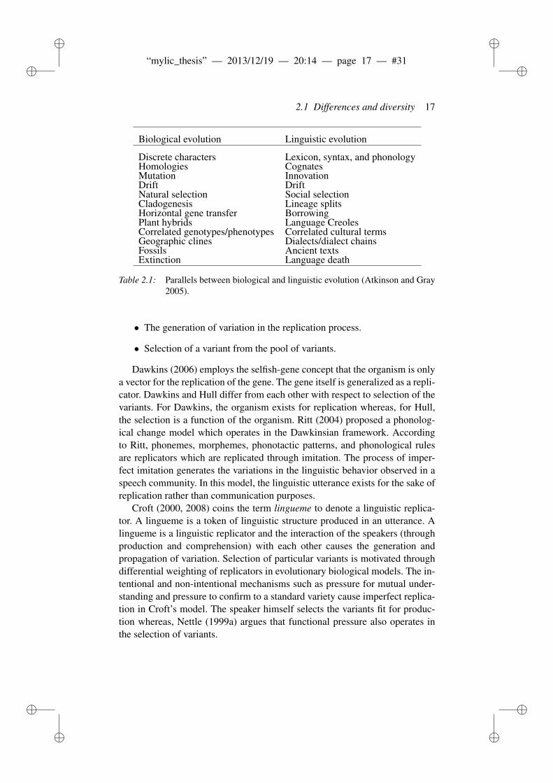
The nineteenth century linguist Schleicher (1853) proposed the stammbaum(family tree) device to show the differences as well as similarities betweenlanguages. Atkinson and Gray (2005) also observe that there has been a cross-pollination of ideas between biology and linguistics before Darwin. Table 2.1summarizes the parallels between biological and linguistic evolution. I preferto see the table as a guideline rather than a hard fact due to the followingreasons:

• Biological drift is not the same as linguistic drift. Biological drift is ran-dom change in gene frequencies whereas linguistic drift is the tendencyof a language to keep changing in the same direction over several gener-ations (Trask 2000: 98).

• Ancient texts do not contain all the necessary information to assist acomparative linguist in drawing the language family history but a suf-ficient sample of DNA (extracted from a well-preserved fossil) can becompared to other biological family members to draw a family tree. Forinstance, the well-preserved finger bone of a species of Homo family(from Denisova cave in Russia; henceforth referred to as Denisovan)was compared to Neanderthals and modern humans. The comparisonshowed that Neanderthals, modern humans, and Denisovans shared acommon ancestor (Krause et al. 2010).

Croft (2008) summarizes the various efforts to explain the linguistic differ-ences in the framework of evolutionary linguistics. Croft also notes that histor-ical linguists have employed biological metaphors or analogies to explain lan-guage change and then summarized the various evolutionary linguistic frame-works to explain language change. In evolutionary biology, some entity repli-cates itself either perfectly or imperfectly over time. The differences resultingfrom imperfect replication leads to differences in a population of species whichover the time leads to splitting of the same species into different species. Theevolutionary change is a two-step process:

ii


ii

ii

2.1 Differences and diversity 17

Biological evolution Linguistic evolution

Discrete characters Lexicon, syntax, and phonologyHomologies CognatesMutation InnovationDrift DriftNatural selection Social selectionCladogenesis Lineage splitsHorizontal gene transfer BorrowingPlant hybrids Language CreolesCorrelated genotypes/phenotypes Correlated cultural termsGeographic clines Dialects/dialect chainsFossils Ancient textsExtinction Language death

Table 2.1: Parallels between biological and linguistic evolution (Atkinson and Gray2005).

• The generation of variation in the replication process.

• Selection of a variant from the pool of variants.

Dawkins (2006) employs the selfish-gene concept that the organism is onlya vector for the replication of the gene. The gene itself is generalized as a repli-cator. Dawkins and Hull differ from each other with respect to selection of thevariants. For Dawkins, the organism exists for replication whereas, for Hull,the selection is a function of the organism. Ritt (2004) proposed a phonolog-ical change model which operates in the Dawkinsian framework. Accordingto Ritt, phonemes, morphemes, phonotactic patterns, and phonological rulesare replicators which are replicated through imitation. The process of imper-fect imitation generates the variations in the linguistic behavior observed in aspeech community. In this model, the linguistic utterance exists for the sake ofreplication rather than communication purposes.

Croft (2000, 2008) coins the term lingueme to denote a linguistic replica-tor. A lingueme is a token of linguistic structure produced in an utterance. Alingueme is a linguistic replicator and the interaction of the speakers (throughproduction and comprehension) with each other causes the generation andpropagation of variation. Selection of particular variants is motivated throughdifferential weighting of replicators in evolutionary biological models. The in-tentional and non-intentional mechanisms such as pressure for mutual under-standing and pressure to confirm to a standard variety cause imperfect replica-tion in Croft’s model. The speaker himself selects the variants fit for produc-tion whereas, Nettle (1999a) argues that functional pressure also operates inthe selection of variants.

ii


ii

ii


The iterative mounting differences induced through generations of imper-fect replication cause linguistic diversity. Nettle (1999a: 10) lists three differenttypes of linguistic diversity:

• Language diversity. This is simply the number of languages present ina given geographical area. New Guinea has the highest geographical di-versity with more than 800 languages spoken in a small island whereasIceland has only one language (not counting the immigration in the re-cent history).

• Phylogenetic diversity. This is the number of (sub)families found inan area. For instance, India is rich in language diversity but has onlyfour language families whereas South America has 53 language families(Campbell 2012: 67–69).

• Structural diversity. This is the number of languages found in an areawith respect to a particular linguistic parameter. A linguistic parametercan be word order, size of phoneme inventory, morphological type, orsuffixing vs. prefixing.

A fourth measure of diversity or differences is based on phonology. Lohr(1998: chapter 3) introduces phonological methods for the genetic classifica-tion of European languages. The similarity between the phonetic inventoriesof individual languages is taken as a measure of language relatedness. Lohr(1998) also compares the same languages based on phonotactic similarity toinfer a phenetic tree for the languages. It has to be noted that Lohr’s compar-ison is based on hand-picked phonotactic constraints rather than constraintsthat are extracted automatically from corpora or dictionaries. Rama (2013) in-troduces phonotactic diversity as an index of age of language group and familysize. Rama and Borin (2011) employ phonotactic similarity for the geneticclassification of 11 European languages.

Consider the Scandinavian languages Norwegian, Danish and Swedish. Allthe three languages are mutually intelligible (to a certain degree) yet are calleddifferent languages. How different are these languages or how distant are theselanguages from each other? Can we measure the pair-wise distances betweenthese languages? In fact, Swedish dialects such as Pitemål and Älvdalska areso different from Standard Swedish that they can be counted as different lan-guages (Parkvall 2009).

In an introduction to the volume titled Approaches to measuring linguisticdifferences, Borin (2013b: 4) observes that we need to fix the units of com-parison before attempting to measure the differences between the units. In thefield of historical linguistics, language is the unit of comparison. In the closely

ii


ii

ii

2.2 Language change 19

related field of dialectology, dialectologists work with a much thinner samplesof a single language. Namely, they work with language varieties (dialects) spo-ken in different sites in the geographical area where the language is spoken.5

For instance, a Swedish speaker from Gothenburg can definitely communicatewith a Swedish speaker of Stockholm. However, there are differences betweenthese varieties and a dialectologist works towards charting the dialectal con-tours of a language.

At a higher level, the three Scandinavian languages are mutually intelligibleto a certain degree but are listed as different languages due to political reasons.Consider the inverse case of Hindi, a language spoken in Northern India. Thelanguage extends over a large geographical area but the languages spoken inEastern India (Eastern Hindi) are not mutually intelligible with the languagesspoken in Western India (Western Hindi). Nevertheless, these languages arereferred to as Hindi (Standard Hindi spoken by a small section of the NorthernIndian population) due to political reasons (Masica 1993).

2.2 Language change

Language changes in different aspects: phonology, morphology, syntax, mean-ing, lexicon, and structure. Historical linguists gather evidence of languagechange from all possible sources and then use the information to classify lan-guages. Thus, it is very important to understand the different kinds of languagechange for the successful computational modeling of language change. In thissection, the different processes of language change are described through ex-amples from the Indo-European and Dravidian language families. Each de-scription of a type of language change is followed by a description of the com-putational modeling of the respective language change.

2.2.1 Sound change

Sound change is the most studied of all the language changes (Crowley andBowern 2009: 184). The typology of sound changes described in the followingsubsections indicate that the sound changes depend on the notions of positionin the word, its neighboring sounds (context) and the quality of the sound in fo-cus. The typology of the sound changes is followed by a subsection describingthe various string similarity algorithms which model different sound changes

5Doculect is the term that has become current and refers to a language variant described ina document.

ii


ii

ii


and hence, employed in computing the distance between a pair of cognates, aproto-form and its reflexes.

2.2.1.1 Lenition and fortition

Lenition is a sound change where a sound becomes less consonant like. Con-sonants can undergo a shift from right to left on one of the scales given belowin Trask (1996: 56).• geminate > simplex.• stop > fricative > approximant• stop > liquid.• oral stop > glottal stop• non-nasal > nasal• voiceless > voicedA few examples (from Trask 1996) involving the movement of sound ac-

cording to the above scales is as follows. Latin cuppa ‘cup’ > Spanish copa.Rhotacism, /s/ > /r/, in Pre-Latin is an example of this change where *flosis >floris genitive form of ‘flower’. Latin faba ‘bean’ > Italian fava is an exampleof fricativization. Latin strata > Italian strada ‘road’ is an example of voicing.The opposite of lenition is fortition where a sound moves from left to right oneach of the above scales. Fortition is not as common as lenition. For instance,there are no examples showing the change of a glottal stop to an oral stop.

2.2.1.2 Sound loss

Apheresis. In this sound change, the initial sound in a word is lost. An exampleof such change is in a South-Central Dravidian language, Pengo. The word inPengo racu ‘snake’ < *tracu.Apocope. A sound is lost in the word-final segment in this sound change. Anexample is: French lit > /li/ ‘bed’.Syncope. A sound is lost from the middle of a word. For instance, Old Indo-Aryan pat.t.a ‘slab, tablet’ ~ Vedic Sanskrit pattra- ‘wing/feather’ (Masica 1993:157).Cluster reduction. In this change a complex consonant cluster is reduced toa single consonant. For instance, the initial consonant clusters in English aresimplified through the loss of h; hring > ring, hnecca > neck (Bloomfield 1935:370). Modern Telugu lost the initial consonant when the initial consonant clus-ter was of the form Cr. Thus Cr > r : vrayu > rayu ‘write’ (Krishnamurti andEmeneau 2001: 317).

ii


ii

ii


Haplology. When a sound or group of sounds recur in a word, then one ofthe occurrence is dropped from the word. For instance, the Latin word nutrixwhich should have been nutri-trix ‘nurse’, regular feminine agent-noun fromnutrio ‘I nourish’ where tri is dropped in the final form. A similar example isLatin stipi-pendium ‘wage-payment’ > stipendium (Bloomfield 1935: 391).

2.2.1.3 Sound addition

Excrescence. When a consonant is inserted between two consonants. For in-stance, Cypriot Arabic developed a [k] as in *pjara > pkjara (Crowley andBowern 2009: 31).Epenthesis. When a vowel is inserted into a middle of a word. Tamil inserts avowel in complex consonant cluster such as paranki < Franco ‘French man,foreigner’ (Krishnamurti 2003: 478).Prothesis. A vowel is inserted at the beginning of a word. Since Tamil phonol-ogy does not permit liquids r, l to begin a word, it usually inserts a vowel ofsimilar quality of that of the vowel present in the successive syllable. Tamilulakam < Sanskrit lokam ‘world’, aracan < rajan ‘king’ (Krishnamurti 2003:476).

2.2.1.4 Metathesis

Two sounds swap their position in this change. Proto-Dravidian (PD) did notallow apical consonants such as t., t

¯, l, l., z. , r in the word-initial position. How-

ever, Telugu allows r, l in the word-initial position. This exception developeddue to the process of metathesis. For instance, PD *iran. t.u > ren. d. u ‘two’ wherethe consonant [r] swapped its position with the preceding vowel [i] (Krish-namurti 2003: 157). Latin miraculum > Spanish milagro ‘miracle’ where theliquids r, l swapped their positions (Trask 2000: 211).

2.2.1.5 Fusion

In this change, two originally different sounds become a new sound where thenew sound carries some of the phonetic features from the two original sounds.For instance, compensatory lengthening is a kind of fusion where after the lossof a consonant, the vowel undergoes lengthening to compensate for the loss inspace (Crowley and Bowern 2009). Hindi ag < Prakrit aggi ‘fire’ is an exampleof compensatory lengthening.

ii


ii

ii


2.2.1.6 Vowel breaking

A vowel can change into a diphthong and yields an extra glide which can bebefore- (on-glide) or off-glide. An example from Dravidian is the Proto-SouthDravidian form *ot.ay > Toda war. ‘to break’; *o > wa before -ay.

2.2.1.7 Assimilation

In this sound change, a sound becomes more similar to the sound preceding orafter it. In some cases, a sound before exactly the same as the sound next to it –complete assimilation; otherwise, it copies some of the phonetic features fromthe next sound to develop into a intermediary sound – partial assimilation. ThePrakrit forms in Indo-Aryan show complete assimilation from their Sanskritforms: agni > aggi ‘fire’, hasta > hatta ‘hand’, and sarpa > sappa ‘snake’.6

Palatalization is a type of assimilation where a consonant preceding a frontvowel develops palatal feature, such as [k] > [c]. For example, Telugu showspalatalization from PD: Telugu ceyi ‘hand’< *key < *kay (Krishnamurti 2003:128).

2.2.1.8 Dissimilation

This sound change is opposite to that of assimilation. A classic case of dissimi-lation is the Grassmann’s law in Sanskrit and Ancient Greek, which took placeindependently. Grassmann’s law states that whenever two syllables immediateto each other had a aspirated stop, the first syllable lost the aspiration. For ex-ample, Ancient Greek thriks ‘hair’ (nominative), trikhos (genitive) as opposedto thrikhos (Trask 2000: 142).

2.2.1.9 Some important sound changes

This subsection deals with some identified sound changes from the Indo-Europ-ean and the Dravidian family. These sound changes are quite famous and wereoriginally postulated as laws, i.e. exceptionless patterns of development. How-ever, there were exceptions to these sound laws which made them recurrentbut not exceptionless. The apical displacement is an example of such soundchange in a subset of South-Central Dravidian languages which is on-goingand did not affect many of the lexical items suitable for sound change (Krish-namurti 1978).

6This example is given by B. Lakshmi Bai.

ii


ii

ii


One of the first discovered sound changes in the IE family is Grimm’s law.Grimm’s law deals with the sound change which occurred in all languages ofGermanic branch. The law states that in the first step, the unvoiced plosivesbecame fricatives. In the second step, the voiced aspirated plosives in PIE losttheir aspiration to become unaspirated voiced plosives. In the third and finalstep, the voiced plosives became unvoiced plosives (Collinge 1985: 63). Cog-nate forms from Sanskrit and Gothic illustrate how Grimm’s law applies toGothic, while the Sanskrit forms retain the original state of affairs:

• C {-Voicing, -Aspiration} ~ C {+Continuant}: traya- ~ θreis ‘three’

• C {+Voicing, +Aspiration} ~ C {+Voicing, -Aspiration}: madhya- ~ mid-jis ‘middle’

• C {+Voicing, -Aspiration} ~ C {-Voicing, -Aspiration}: dasa- ~ taihun‘ten’

However, there were exceptions to this law: whenever the voiceless plosivedid not occur in the word-initial position or did not have an accent in the pre-vious syllable, the voiceless plosive became voiced. This is known as Verner’slaw. Some examples of this law are: Sanskrit pitár ~ Old English faedar ‘fa-ther’, Sanskrit (va)vrtimá ~ Old English wurdon ‘to turn’.

The next important sound change in IE linguistics is the Grassmann’s law.As mentioned above, Grassmann’s law (GL) states that whenever two sylla-bles (within the same root or when reduplicated) are adjacent to each other,with aspirated stops, the first syllable’s aspirated stop loses the aspiration. Ac-cording to Collinge (1985: 47), GL is the most debated of all the sound changesin IE. Grassmann’s original law has a second proposition regarding the Indiclanguages where a root with a second aspirated syllable can shift the aspira-tion to the preceding root (also known as aspiration throwback) when followedby a aspirated syllable. Grassmann’s first proposition is mentioned as a lawwhereas, the second proposition is usually omitted from historical linguisticstextbooks.

Bartholomae’s law (BL) is a sound change which affected Proto-Indo-Irani-an roots. This law states that whenever a voiced, aspirated consonant is fol-lowed by a voiceless consonant, there is an assimilation of the following voice-less consonant and deaspiration in the first consonant. For instance, in Sanskrit,labh+ta > labdha ‘sieze’, dah+ta > dagdha ‘burnt’, budh+ta > buddha ‘awak-ened’ (Trask 2000: 38).

Together, BL and GL received much attention due to their order of ap-plication in the Indic languages. One example is the historical derivation ofdughdas in Sanskrit. The first solution is to posit *dhugh+thas BL→ *dhughdhas

ii


ii

ii


GL→ *dughdhasdeaspiration→ dugdhas. Reversing the order of BL and GL yields the

same output. Collinge (1985: 49–52) summarizes recent efforts to explain allthe roots in Indic branch using a particular rule application order of BL andGL. The main take-away from the GL debate is that the reduplication exam-ples show the clearest deaspiration in first syllable. For instance, dh – dh > d –dh in Sanskrit da-dha-ti ‘to set’, reduplicated present. A loss of second syllableaspiration immediately before /s/, /t/ (Beekes 1995: 128). An example of thissound change from Sanskrit is: dáh-a-ti ‘burn’ < PIE *dhagh-, but 3 sg. s-aor.á-dhak < *-dhak-s-t.

An example of the application of BL and GL is: buddha can be explained asPIE *bhewdh (e-grade) GL→ Sanskrit budh (Ø-grade); budh+ta BL→ buddha ‘awak-ened’ (Ringe 2006: 20).

Another well-known sound change in Indo-European family is umlaut (met-aphony). In this change, a vowel transfers some of its phonetic features to itspreceding syllable’s vowel. This sound change explains singular : plural formsin Modern English such as foot : feet, mouse : mice. Trask (2000: 352–353)lists three umlauts in the Germanic branch:

• i-umlaut fronts the preceding syllable’s vowel when present in a pluralsuffix in Old English -iz.

• a-umlaut lowers the vowels [i] > [e], [u] > [o].

• u-umlaut rounds the vowels [i] > [y], [e] > [ø], [a] > [æ].

Kannada, a Dravidian language, shows an umlaut where the mid vowels be-came high vowels in the eighth century: [e] > [i] and [o] > [u], when the nextsyllable has [i] or [u]; Proto-South Dravidian *ket.u > Kannada kid. u ‘to perish’(Krishnamurti 2003: 106).

2.2.1.10 Computational modeling of sound change

Biologists compare sequential data to infer family trees for species (Gusfield1997; Durbin et al. 2002). As noted before, linguists primarily work with wordlists to establish the similarities and differences between languages to infer thefamily tree for a set of related languages. Identification of synchronic wordforms descended from a proto-language plays an important role in compara-tive linguistics. This is known as the task of “Automatic cognate identification”in LT literature. In LT, the notion of cognates is useful in building LT systemssuch as sentence aligners that are used for the automatic alignment of sen-tences in the comparable corpora of two closely related languages. One such

ii


ii

ii


attempt is by Simard, Foster and Isabelle (1993) employ similar words7 aspivots to automatically align sentences from comparable corpora of Englishand French. Covington (1996), in LT, was the first to develop algorithms forcognate identification in the sense of historical linguistics.8 Covington (1996)employs phonetic features for measuring the change between cognates. Therest of the section introduces Levenshtein distance (Levenshtein 1966) and theother orthographic measures for quantifying the similarity between words. Iwill also make an attempt at explaining the linguistic motivation for using thesemeasures and their limitations.

Levenshtein (1966) computes the distance between two strings as the min-imum number of insertions, deletions and substitutions to transform a sourcestring to a target string. The algorithm is extended to handle methathesis byintroducing an operation known as “transposition” (Damerau 1964). The Lev-enshtein distance assigns a distance of 0 to identical symbols and assigns 1 tonon-identical symbol pairs. For instance, the distance between /p/ and /b/ isthe same as the distance between /f/ and /æ/. A linguistic comparison wouldsuggest that the difference between the first pair is in terms of voicing whereasthe difference between the second pair is greater than the first pair. Levenshteindistance (LD) also ignores the positional information of the pair of symbols.The left and right context of the symbols under comparison are ignored in LD.Researchers have made efforts to overcome the shortcomings of LD in directas well as indirect ways. Kessler (2005) gives a summary of various phoneticalgorithms developed for the historical comparison of word forms.

In general, the efforts to make LD (in its plainest form is henceforth referredas “vanilla LD”) sensitive to phonetic distances is achieved by introducing anextra dimension to the symbol comparison. The sensitization is achieved intwo steps:

1. Represent each symbol as a vector of phonetic features.

2. Compare the vectors of phonetic features belonging to the dissimilarsymbols using Manhattan distance, Hamming distance or Euclidean dis-tance.

A feature in a feature vector can be represented as a 1/0 bit or a value on a con-tinuous (Kondrak 2002a) or ordinal (Grimes and Agard 1959) scale. An ordinalscale implies an implicit hierarchy in the phonetic features – place of articula-tion and manner of articulation. Heeringa (2004) uses a binary feature-valued

7Which they refer to as “cognates”, even though borrowings and chance similarities areincluded.

8Grimes and Agard (1959) use a phonetic comparison technique for estimating linguisticdivergence in Romance languages.

ii


ii

ii


system to compare Dutch dialects. Rama and Singh (2009) use the phoneticfeatures of the Devanagari alphabet to measure the language distances betweenten Indian languages.

The sensitivity of LD can also be improved based on the symbol distancesderived from empirical data. In this effort, originally introduced in dialectology(Wieling, Prokic and Nerbonne 2009), the observed frequencies of a symbol-pair is used to assign an importance value. For example, a sound correspon-dence such as /s/ ~ /h/ or /k/ ~ /c/ is observed frequently across the world’s lan-guages (Brown, Holman and Wichmann 2013). However, historical linguistsprefer natural yet, less common-place sound changes to establish subgroups.An example of natural sound change is Grimm’s law described in previous sub-section. In this law, each sound shift is characterized by the loss of a phoneticfeature. An example of unnatural and explainable chain of sound changes is theArmenian erku (cf. section 2.3.1.1). A suitable information-theoretic measuresuch as Point-wise Mutual Information (PMI) – which discounts the common-ality of a sound change – is used to compute the importance for a particularsymbol-pair (Jäger 2014).

List (2012) applies a randomized test to weigh the symbol pairs based onthe relative observed frequencies. His method is successful in identifying casesof regular sound correspondences in English ~ German where German showschanged word forms from the original Proto-Germanic forms due to the HighGerman consonant shift. We are aware of only one effort (Rama, Kolachinaand Kolachina 2013) which incorporates both frequency and context into LDfor cognate identification. Their system recognizes systematic sound corre-spondences between Swedish and English such as /sk/ in sko ‘shoe’ ~ /S/.

An indirect sensitization is to change the input word representation formatto vanilla LD. Dolgopolsky (1986) designed a sound class system based onthe empirical data from 140 Eurasian languages. Brown et al. (2008) devised asound-class system consisting of 32 symbols and few post-modifiers to com-bine the previous symbols and applied vanilla LD to various tasks in historicallinguistics. One limitation of LD can be exemplified through the Grassmann’sLaw example. Grassmann’s law is a case of distant dissimilation which cannotbe retrieved by LD.

There are string similarity measures which work at least as well as LD.A few such measures are Dice, Longest common subsequence ratio (Tiede-mann 1999), and Jaccard’s measure. Dice and Jaccard’s index are related mea-sures which can handle a long-range assimilation/dissimilation. Dice countsthe common number of bigrams between the two words. Hence, bigrams arethe units of comparison in Dice. Since bigrams count successive symbols, bi-grams can be replaced with more generalized skip-grams which count n-gramsof any length and any number of skips. In some experiments whose results are

ii


ii

ii


not presented here, skip-grams perform better than bigrams in the task of cog-nate identification.

The Needleman-Wunsch algorithm (Needleman and Wunsch 1970) is thesimilarity counterpart of Levenshtein distance. Eger (2013) proposes contextand PMI-based extensions to the original Needleman-Wunsch algorithm forthe purpose of letter-to-phoneme conversion for English, French, German, andSpanish.

2.2.2 Semantic change

Semantic change characterizes the change in the meaning of a linguistic form.Although textbooks (Campbell 2004; Crowley and Bowern 2009; Hock andJoseph 2009) usually classify semantic change under the change of meaning ofa lexical item, Fortson (2003) observes that semantic change also includes lex-ical change and grammaticalization. Trask (2000: 300) characterizes semanticchange as one of the most difficult changes to identify. Lexical change in-cludes introduction of new lexical items into language through the processesof borrowing (copying), internal lexical innovation, and shortening of words(Crowley and Bowern 2009: 205–209). Grammaticalization is defined as theassignment of a grammatical function to a previously lexical item. Grammat-icalization is usually dealt under the section of syntactic change. Similarly,structural change such as basic word order change, morphological type or erga-tivity vs. accusativity is also included under syntactic change (Crowley andBowern 2009; Hock and Joseph 2009).

2.2.2.1 Typology of semantic change

The examples in this section come from Luján 2010 and Fortson 2003 exceptfor the Dravidian example which is from Krishnamurti 2003: 128.

1. Broadening and narrowing. A lexical item’s meaning can undergo a shiftto encompass a much wider range of meaning in this change. Originally,dog meant a particular breed of dog and hound meant a generic dog. Theword dog underwent a semantic change to mean not a particular breedof dog but any dog. Inversely, the original meaning of hound changedfrom ‘dog’ to ‘hunting dog’. The original meaning of meat is ‘food’ inthe older forms of English. This word’s meaning has now changed tomean only ‘meat’ and still survives in expressions such as sweetmeatand One man’s meat is another man’s poison. Tamil kili ‘bird’ ~ Teluguchili- ‘parrot’ is another example of narrowing.

ii


ii

ii


2. Melioration and pejoration. In pejoration, a word with non-negativemeaning acquires a negative meaning. For instance, Old High Germandiorna/thiorna ‘young girl’ > Modern High German dirne ‘prostitute’.Melioration is the opposite of pejoration where a word acquires a morepositive meaning than its original meaning. For instance, the originalEnglish word nice ‘simple, ignorant’ > ‘friendly, approachable’.

3. Metaphoric extension. In this change, a lexical item’s meaning is ex-tended through the employment of a metaphor such as body parts: head‘head of a mountain’, tail ‘tail of a coat’; heavenly objects: star ‘rock-star’; resemblance to objects: mouse ‘computer mouse’.

4. Metonymic extension. The original meaning of a word is extended throu-gh a relation to the original meaning. The new meaning is somehowrelated to the older meaning such as Latin sexta ‘sixth (hour)’ > Spanishsiesta ‘nap’, Sanskrit ratha ‘chariot’ ~ Latin rota ‘wheel’.

2.2.2.2 Lexical change

Languages acquire new words through the mechanism of borrowing and neol-ogisms. Borrowing is broadly categorized into lexical borrowing (loanwords)and loan translations. Lexical borrowing usually involves introduction of a newword from the donor language to the recipient language. Examples of suchborrowings are the word beef ‘cow’ from Norman French. Although Englishhad a native word for cow, the meat was referred to as beef and was sub-sequently internalized into the English language. English borrowed a largenumber of words through cultural borrowing. Examples of such words arechocolate, coffee, juice, pepper, and rice. The loanwords are often modifiedto suit the phonology and morphology of the recipient language. For instance,Dravidian languages tend to deaspirate the aspirate sounds in the loanwordsborrowed from Sanskrit: Tamil metai < Sanskrit medha ‘wisdom’ and Telugukata < Sanskrit katha ‘story’.

Meanings can also be borrowed into a language and such cases are calledcalques. For instance, Telugu borrowed the concept of black market and trans-lated it as nalla bajaru. Neologisms is the process of creating new words torepresent hitherto unknown concepts – blurb, chortle; from person names –volt, ohm, vandalize (from Vandals); place names – Swedish persika ‘peach’ <Persia; from compounding – braindead; from derivation – boombox; amalga-mation – altogether, always, however; from clipping – gym < gymnasium, bike< bicycle, and nuke < nuclear.

ii


ii

ii


2.2.2.3 Grammatical change

Grammatical change is a cover term for morphological change and syntacticchange taken together. Morphological change is defined as change in the mor-phological form or structure of a word, a word form or set of such word forms(Trask 2000: 139–40, 218). A sub-type of morphological change is remor-phologization where a morpheme changes its function from one to another. Asound change might effect the morphological boundaries in a word causing themorphemes to be reanalysed as different morphemes from before. An exam-ple of such change is English umlaut which caused irregular singular : pluralforms such as foot : feet, mouse : mice. The reanalysis of the morphemes can beextended to words as well as morphological paradigms resulting in a restruc-turing of the morphological system of the language. The changes of extensionand leveling are traditionally treated under analogical change (Crowley andBowern 2009: 189–194).

Syntactic change is the change of syntactic structure such as the word or-der (markedness shift in word-order), morphological complexity (from inflec-tion to isolating languages), verb chains (loss of free verb status to pre- orpost-verbal modifiers), and grammaticalization. It seems quite difficult to drawa line between where a morphological change ends and a syntactic changestarts.9 Syntactic change also falls within the investigative area of linguistic ty-pology. Typological universals act as an evaluative tool in comparative linguis-tics (Hock 2010: 59). Syntactic change spreads through diffusion/borrowingand analogy. Only one syntactic law has been discovered in Indo-Europeanstudies called Wackernagel’s law, which states that enclitics originally occu-pied the second position in a sentence (Collinge 1985: 217).

2.2.2.4 Computational modeling of semantic change

The examples given in the previous section are about semantic change froman earlier form of the language to its current form. The Dravidian exampleof change from Proto-Dravidian *kil-i ‘bird’ > Telugu ‘parrot’ is an exampleof a semantic shift which occurred in a daughter language (Telugu) from theProto-Dravidian’s original meaning of ‘bird’.

The work of Kondrak 2001, 2004, 2009 attempts to quantify the amount ofsemantic change in four Algonquian languages. Kondrak used Hewson’s Al-gonquian etymological dictionary (Hewson 1993) to compute the phonetic aswell as semantic similarity between the cognates of the four languages. As-

9Fox (1995: 111) notes that “there is so little in semantic change which bears any relation-ship to regularity in phonological change”.

ii


ii

ii


suming that the languages under study have their own comparative dictionary,Kondrak’s method works at three levels:

• Gloss identity. Whenever two word forms in the dictionary have identi-cal meanings, the word forms get a semantic similarity score of 1.0.

• Keyword identity. In this step, glosses are POS-tagged with an existingPOS-tagger and only the nouns (NN tagged) are supposed to carry mean-ing. This step restricts the comparison of grammatically over-loadedforms and the identification of grammaticalization.

• WordNet similarity. In this step, the keywords identified through theprevious step are compared through the WordNet structure (Fellbaum1998). The sense distance is computed using a semantic similarity mea-sure such as Wu-Palmer’s measure, Lin’s similarity, Resnik Similarity,Jiang-Conrath distance, and Leacock-Chodorow similarity (Jurafsky andMartin 2000: chapter 20.6).

The above procedure of computing semantic distance is combined with a pho-netic similarity measure called ALINE (Kondrak 2000). The combination ofphonetic and semantic similarities is shown to perform better than the individ-ual similarity measures. There were few other works to compute semantic dis-tance between languages based on bilingual dictionaries (Cooper 2008; Egerand Sejane 2010).

The major deficiency in Kondrak’s work is the restriction on the mobilityof meaning across syntactic categories and the restriction to nouns. In con-trast, comparative linguists also work with comparing and reconstructing ofbound morphemes and their functions. Moreover, grammaticalization is notrecognized in this framework. Finally, Kondrak’s algorithms require compara-tive dictionaries as an input, which require a great deal of human effort. Thisseems to be remedied to a certain extent in the work of Tahmasebi (2013) andTahmasebi and Risse (under submission).

Unlike Kondrak, Tahmasebi works on the diachronic texts of a single lan-guage. Tahmasebi’s work attempts at identifying the contents and interpretingthe context in which the contents occur. This work identifies two importantsemantic changes, namely word sense change and named entity change. Au-tomatic identification of toponym change is a named entity related task. Anexample of named entity change is the reversal of city and town names, inRussia after the fall of Soviet Union, to their early or pre-revolutionary eranames such as Leningrad > St. Petersburg (also Petrograd briefly); Stalingrad(earlier Tsaritsyn) > Volgograd.

ii


ii

ii

2.3 How do historical linguists classify languages? 31

2.3 How do historical linguists classify languages?

Historical linguists classify languages through comparison of related languagesbased on diagnostic evidence. The most important tool in the toolkit of his-torical linguists is the comparative method. The comparative method worksthrough the comparison of vocabulary items and grammatical forms to iden-tify the systematic sound correspondences (cf. sections 2.2.1 and 2.2.2 for asummary of sound change and semantic change) between the languages andthen project those sound correspondences to intermediary ancestral languagesand further back, to a proto-language. The comparative method also recon-structs the phonemes (phonological system), morphemes (morphological sys-tem), syntax, and meanings in the intermediary ancestral languages – such asProto-Germanic. These intermediary languages are then used to reconstructthe single ancestral language such as Proto-Indo-European. The comparativemethod also identifies the shared innovations (sound changes which are sharedamong a subset of related languages under study) to assign a internal structure(a branching structure) to the set of related languages. This task comes underthe label of subgrouping. Overall, the application of the comparative methodresults in the identification of relations between languages and an assignmentof tree structure to the related languages. However, the comparative method isnot without problems. The comparative method works by following the tracesleft by the processes of language change. Unlike biology the traces of the ear-lier language changes might be covered or obliterated by temporally recentchanges. Thus the comparative method will not be able to recover the origi-nal forms whenever the change did not leave a trace in the language. This isknown as the time limit of the comparative method (Harrison 2003) where thecomparative method does not work for recovering temporally deep – greaterthan 8000 years (Nichols 1992) – language change.

The rest of the section describes the ingredients which go into the compar-ative method, models of language change, examples of how few families wereestablished through the comparative method, and the mechanized parts of thecomparative method.

2.3.1 Ingredients in language classification

The history of the idea of language relationships, from the sixteenth and sev-enteenth centuries is summarized by Metcalf (1974: 251) (from Hoenigswald1990: 119) as follows:

First, [. . . ] there was “the concept of a no longer spoken parent language

ii


ii

ii


which in turn produced the major linguistic groups of Asia and Europe.”Then there was [. . . ] “a concept of the development of languages intodialects and of dialects into new independent languages.” Third came“certain minimum standards for determining what words are borrowedand what words are ancestral in a language,” and, fourth, “an insistencethat not a few random items, but a large number of words from the basicvocabulary should form the basis of comparison” [. . . ] fifth, the doctrinethat “grammar” is even more important than words; sixth, the idea thatfor an etymology to be valid the differences in sound – or in “letters” –must recur, under a principle sometimes referred to as “analogia”.

The above quote stresses the importance of selection of basic vocabularyitems for language comparison and superiority of grammatical evidence oversound correspondences for establishing language relationships. The next sub-section describes the selection process of vocabulary items and examples ofgrammatical correspondences for positing language relationships.

2.3.1.1 Three kinds of evidence

Meillet (1967: 36) lists three sources of evidence for positing language re-lationships: sound correspondences obtained from phonology, morphologicalcorrespondences, and similarities in basic vocabulary. Basic lexical compari-son precedes phonological and morphological evidence during the process ofproposal and consolidation of language relationships.

Campbell and Poser (2008: 166) insist on the employment of basic vocab-ulary for lexical comparison. Curiously, the notion of basic vocabulary wasnot established on empirical grounds. Basic vocabulary is usually understoodto consist of terms for common body parts, close kin, astronomical objects,numerals from one to ten, and geographical objects. The strong assumptionbehind the choice of basic vocabulary is that these vocabulary items are veryresistant to borrowing, lexical replacement, and diffusion and hence, show theevidence of a descent from a common ancestor. However, basic vocabularycan also be borrowed. For instance, Telugu borrowed lexical items for ‘sun’,‘moon’, and ‘star’ – surya, candra, and nakshatra – from Indo-Aryan lan-guages, and the original Dravidian lexemes – end. a, nela, and cukka – becameless frequent or were relegated to specific contexts. Brahui, a Dravidian lan-guage surrounded by Indo-Aryan languages, also borrowed quite a large num-ber of basic vocabulary items.

The second evidence for language relationship comes from sound corre-spondences. Sound correspondences should be recurrent and not sporadic. The

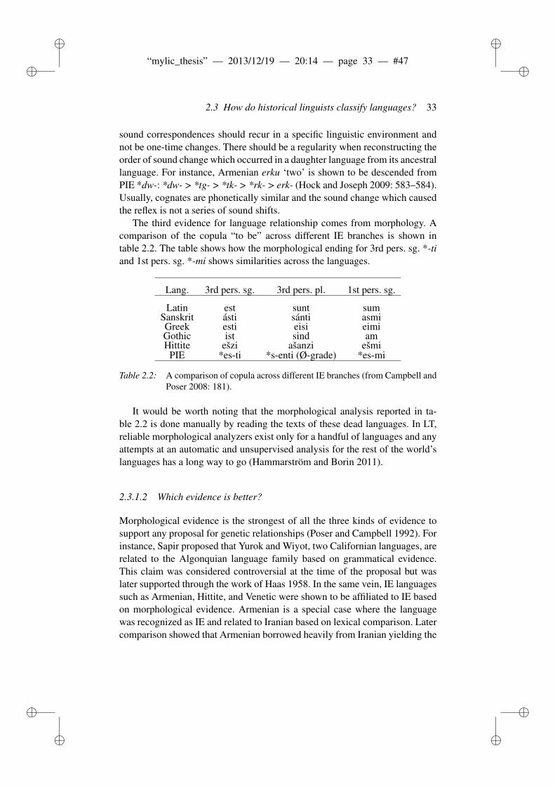
ii


ii

ii


sound correspondences should recur in a specific linguistic environment andnot be one-time changes. There should be a regularity when reconstructing theorder of sound change which occurred in a daughter language from its ancestrallanguage. For instance, Armenian erku ‘two’ is shown to be descended fromPIE *dw-: *dw- > *tg- > *tk- > *rk- > erk- (Hock and Joseph 2009: 583–584).Usually, cognates are phonetically similar and the sound change which causedthe reflex is not a series of sound shifts.

The third evidence for language relationship comes from morphology. Acomparison of the copula “to be” across different IE branches is shown intable 2.2. The table shows how the morphological ending for 3rd pers. sg. *-tiand 1st pers. sg. *-mi shows similarities across the languages.

Lang. 3rd pers. sg. 3rd pers. pl. 1st pers. sg.

Latin est sunt sumSanskrit ásti sánti asmiGreek esti eisi eimiGothic ist sind amHittite ešzi ašanzi ešmi

PIE *es-ti *s-enti (Ø-grade) *es-mi

Table 2.2: A comparison of copula across different IE branches (from Campbell andPoser 2008: 181).

It would be worth noting that the morphological analysis reported in ta-ble 2.2 is done manually by reading the texts of these dead languages. In LT,reliable morphological analyzers exist only for a handful of languages and anyattempts at an automatic and unsupervised analysis for the rest of the world’slanguages has a long way to go (Hammarström and Borin 2011).

2.3.1.2 Which evidence is better?

Morphological evidence is the strongest of all the three kinds of evidence tosupport any proposal for genetic relationships (Poser and Campbell 1992). Forinstance, Sapir proposed that Yurok and Wiyot, two Californian languages, arerelated to the Algonquian language family based on grammatical evidence.This claim was considered controversial at the time of the proposal but waslater supported through the work of Haas 1958. In the same vein, IE languagessuch as Armenian, Hittite, and Venetic were shown to be affiliated to IE basedon morphological evidence. Armenian is a special case where the languagewas recognized as IE and related to Iranian based on lexical comparison. Latercomparison showed that Armenian borrowed heavily from Iranian yielding the

ii


ii

ii


earlier conclusion that Armenian is a language within Iranian subfamily. Latergrammatical comparison, however, showed that Armenian is a distinct sub-group within the IE family. When working with all three kinds of evidencethe linguist seeks to eliminate borrowings and other spurious similarities whenconsolidating new genetic proposals. In a computational study involving theancient languages of the IE family, Nakhleh et al. (2005) perform experimentson differential weighting of phonological, morphological, and lexical charac-ters to infer the IE family tree. They find that weighting improves the matchof the inferred tree with the known IE tree. Kolachina, Rama and Bai (2011)apply the maximum parsimony method to hand-picked features in the Dravid-ian family to weigh the binary vs. ternary splitting hypotheses at the top-mostnode.

2.3.2 The comparative method and reconstruction

The previous subsection introduced the three sources for accumulating ev-idence for consolidating the genetic relation proposals between languages.This section summarizes the working of comparative method and the proce-dure for reconstructing the proto-language as well as the intermediary proto-languages. The comparative method has been described in various articles byHoenigswald (1963, 1973, 1990, 1991), Durie and Ross (1996), and Rankin(2003). The flowchart in figure 2.1 presents an algorithmic representation ofthe steps involved in the comparative method. The rest of the section summa-rizes the various steps and the models of language change with illustrations.

Comparison of basic vocabulary constitutes the first step in the comparativemethod. In this step the basic word forms are compared to yield a list of soundcorrespondence sets. The sound correspondences should be recurring and notan isolated pair such as Greek /th/ ~ Latin /d/ in theos ~ deus (Fox 1995: 66) –we know that Greek /th/ should correspond to Latin /f / in word-initial position.These sound correspondences are then used to search for plausible cognatesacross the languages. Meillet requires that a plausible cognate should occurin at least three languages to label the cognate set as plausible. In the nextstep, a possible proto-phoneme for a sound correspondences set is posited. Forinstance, if a sound correspondence set is of the form p/p/p, in the Latin, Greek,and Sanskrit words for ‘father’, then the proto-phoneme is posited as *p. Inthe next step, a phonetic value is assigned to the proto-phoneme. The case ofp/p/p is a relatively easy one whereas the case of Latin formus, Greek thermos,and Sanskrit gharmas ‘warm’ is a recurring sound correspondence of f /th/gh.In this case, a consensual phonetic value is assigned to the proto-phoneme.The actual reconstructed proto-phoneme is *gwh. This reconstruction comes

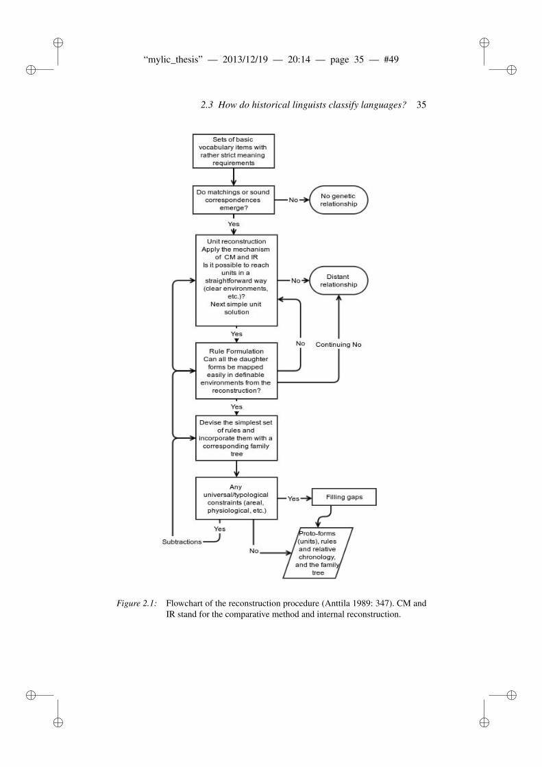
ii


ii

ii


Figure 2.1: Flowchart of the reconstruction procedure (Anttila 1989: 347). CM andIR stand for the comparative method and internal reconstruction.

ii


ii

ii


at a later stage when the proto-phonemes of natural type are established. Forinstance, even when Armenian erk- regularly corresponds to Sanskrit dw- inword-initial position, the explanation for such regularity is left for the laterstage. Anttila (1989) calls such regular yet non-gradual similarity an evidencefor distant relationship. It has to be noted that the assigned phonetic valueof a proto-phoneme should not be of any arbitrary value but something thatexplains the gradual phonetic shift and the change from a proto-phoneme toreflexes should be explainable in the least number of most natural changes,also referred to as Occam’s Razor.

As noted earlier, regular morphological correspondence provides the strong-est evidence for genetic relationship. In fact, Meillet (translated by Poser andCampbell 1992) holds that regular sound correspondences are not the absoluteproof of relatedness and goes on to stress that irregular grammatical forms arethe best evidence for establishing a common language. According to Anttila(1989), what passes as morphological reconstruction is mostly phonologicalin nature (morphophonemic analysis). Morphophonemic reconstruction makesup the reconstruction of grammatical forms and their grammatical function.

The reconstruction of the lexicon or the meaning of the reconstructed proto-forms is not parallel to that of phonological reconstruction. According to Fox(1995: 111–118), the lexicon reconstruction procedure does not have the par-allel step of positing a proto-meaning. The next step after the comparison ofdaughter languages’ meanings is the reconstruction of the proto-meanings. Aexample of such reconstruction are the assignment of meaning to the IE proto-form *pont. Greek has two meanings ‘sea’ and ‘path’; Latin and Armenianhave meanings ‘ford’ and ‘bridge’; Sanskrit and Old Church Slavonic have themeanings of ‘road’ or ‘path’. Vedic has the meaning of ‘passage’ through air aswell. A reconciliation of these different meanings would indicate that the orig-inal form had the meaning of ‘passage’ which was extended to ‘sea’ in Greek,a narrowing of travel over water or land in Latin and Armenian. So, the origi-nal meaning of *pont is reconstructed as a general word for travel. In English,little and small are different (roughly synonymous) lexical items, whereas inSwedish the cognate forms liten and små are inflectional forms of the samelexical item (liten, litet, lilla, lille are singular forms and små is plural).10 Toconclude, the lexicon reconstruction is done on a per-word basis and is not asstraightforward as phonological reconstruction.

Typological universals serve as a sanity check against the reconstructed lan-guages’ linguistic systems. For instance, positing an unbalanced vowel or con-sonant system would be untenable under known typological universals. Hock(2010: 60) summarizes the ‘glottalic’ theory in Indo-European languages as

10This example is given by Lars Borin.

ii


ii

ii


an example of typological check against the reconstructed consonant system.The PIE consonant inventory which was once the most widely accepted hada voiceless, voiced, and voiced aspirate consonants. This system was assertedas typologically impossible since any language with voiced aspirates shouldalso have voiceless aspirates. A glottalized consonant series in addition to thevoiceless aspirates was proposed as the alternate reconstruction that satisfiesthe conditions imposed by typology. Working from PIE to the daughter lan-guages, the expanded consonant system would reject Grimm’s law and sug-gests that the Germanic and Armenian consonant systems preserve the originalPIE state and all the other IE languages have undergone massive shifts fromPIE. The glottalic system has been discredited after the discovery of Indone-sian languages which have voiced aspirates without their voiceless counter-parts. Moreover the glottalic system is against the general principle of Occam’sRazor (Hock and Joseph 2009: 443–445).

The regular sound correspondences established through the comparativemethod also help in recognizing borrowings. For instance, English has twoforms with meanings related to ‘brother’ brotherly and fraternal. The regularsound correspondence of PIE *bh > b suggests that the f in fraternal is not anative word but was borrowed from Latin.

In this step, the enumeration of shared innovations and shared retentionsform the next stage for positing a family tree. Shared innovations are regularand natural sound changes shared by a subset of languages. The shared inno-vations in a subset of languages suggest that these languages have descendedfrom a intermediary common ancestor which has undergone this particular lin-guistic change and all the daughter languages of the ancestor show this change.Grimm’s law is such a sound change which groups all the Germanic languagesunder a single node. Meillet (1967: 36) employs a different term shared aber-rancies (also called shared idiosyncrasies by Hock and Joseph 2009: 437) suchas the recurrent suppletive form correspondence between English and Germanfor a strong evidence of the genetic relationship.

Despite the copious research in IE linguistics, the tree structure for IE athigher levels is not very well resolved (cf. figure 2.2). A basic assumption ofthe comparative method is that the proto-language is uniform and without di-alectal variation. However, there are unexplainable reflexes which cannot beaccounted for from known evidence. In such a case, a practitioner of the com-parative method has to admit it as dialectal variation. An example of the admit-tance of dialectal variation in proto-language is the correspondence of voice-less aspirates in Indo-Iranian to other IE branches: Sanskrit ratha- ~ Latin rota‘chariot, wheel’. Finally, the comparative method assumes that sound changeoperates without exceptions or it affects all the suitable lexical items. However,Krishnamurti (1978) demonstrated a sound change such as apical displacement

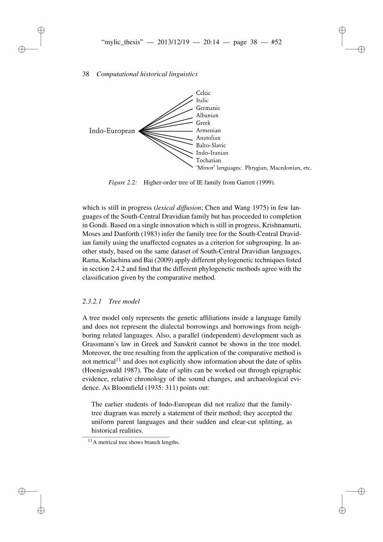
ii


ii

ii


Figure 2.2: Higher-order tree of IE family from Garrett (1999).

which is still in progress (lexical diffusion; Chen and Wang 1975) in few lan-guages of the South-Central Dravidian family but has proceeded to completionin Gondi. Based on a single innovation which is still in progress, Krishnamurti,Moses and Danforth (1983) infer the family tree for the South-Central Dravid-ian family using the unaffected cognates as a criterion for subgrouping. In an-other study, based on the same dataset of South-Central Dravidian languages,Rama, Kolachina and Bai (2009) apply different phylogenetic techniques listedin section 2.4.2 and find that the different phylogenetic methods agree with theclassification given by the comparative method.

2.3.2.1 Tree model

A tree model only represents the genetic affiliations inside a language familyand does not represent the dialectal borrowings and borrowings from neigh-boring related languages. Also, a parallel (independent) development such asGrassmann’s law in Greek and Sanskrit cannot be shown in the tree model.Moreover, the tree resulting from the application of the comparative method isnot metrical11 and does not explicitly show information about the date of splits(Hoenigswald 1987). The date of splits can be worked out through epigraphicevidence, relative chronology of the sound changes, and archaeological evi-dence. As Bloomfield (1935: 311) points out:

The earlier students of Indo-European did not realize that the family-tree diagram was merely a statement of their method; they accepted theuniform parent languages and their sudden and clear-cut splitting, ashistorical realities.

11A metrical tree shows branch lengths.

ii


ii

ii


The above statement suggests that the tree is only a model or device to repre-sent the inherited linguistic characteristics from a common ancestor. Moreover,the comparative method attempts to establish a successive split model of a lan-guage family. Thus, a resolved family tree need not show binary splits at allthe nodes – the Dravidian family tree shows a ternary split at the root (Krish-namurti 2003: 493). A mathematical treatment of the enumeration of possiblerooted binary vs. non-binary trees is given by Felsenstein (2004: 19–36). Thenumber of possible rooted, non-binary, and unlabeled trees for a given familysize is presented in table 2.3.

Family size Tree shapes

2 15 1210 231220 25673875140 9.573×1018

80 3.871×1040

100 2.970×1051

Table 2.3: Number of non-binary tree topologies.

2.3.2.2 Wave model

The observation that there were similarities across the different branches of theIE family led to the wave model, proposed by Schmidt (1872). The IE wavemodel is given in figure 2.3. For instance, the Balto-Slavic, Indo-Iranian, andArmenian subfamilies share the innovation from original velars to palatals. Inthis model, an innovation starts out in a speech community and diffuses outto neighboring speech communities. An example of an isogloss map for SouthDravidian languages is given in figure 2.4. The wave model is not an alternativeto the tree model but captures the points not shown by the tree model. The wavemodel captures the overlapping innovations across the subfamilies and alsoshows the non-homogeneity of the proto-language. Representing the proto-language at one end and dialects of a daughter language at the other end on agraded scale, the tree model can be re-conciliated with the wave model. Thetree-envelope representation of Southworth 1964 is one such example whichattempts at showing the subgrouping as well as the shared innovations betweenthe subgroups. The study of lexical diffusion of s > h > Ø in Gondi dialectsby Krishnamurti (1998) is an example where the original Proto-Dravidian *c> *s in the word-initial, pre-vocalic position completed the sound change in

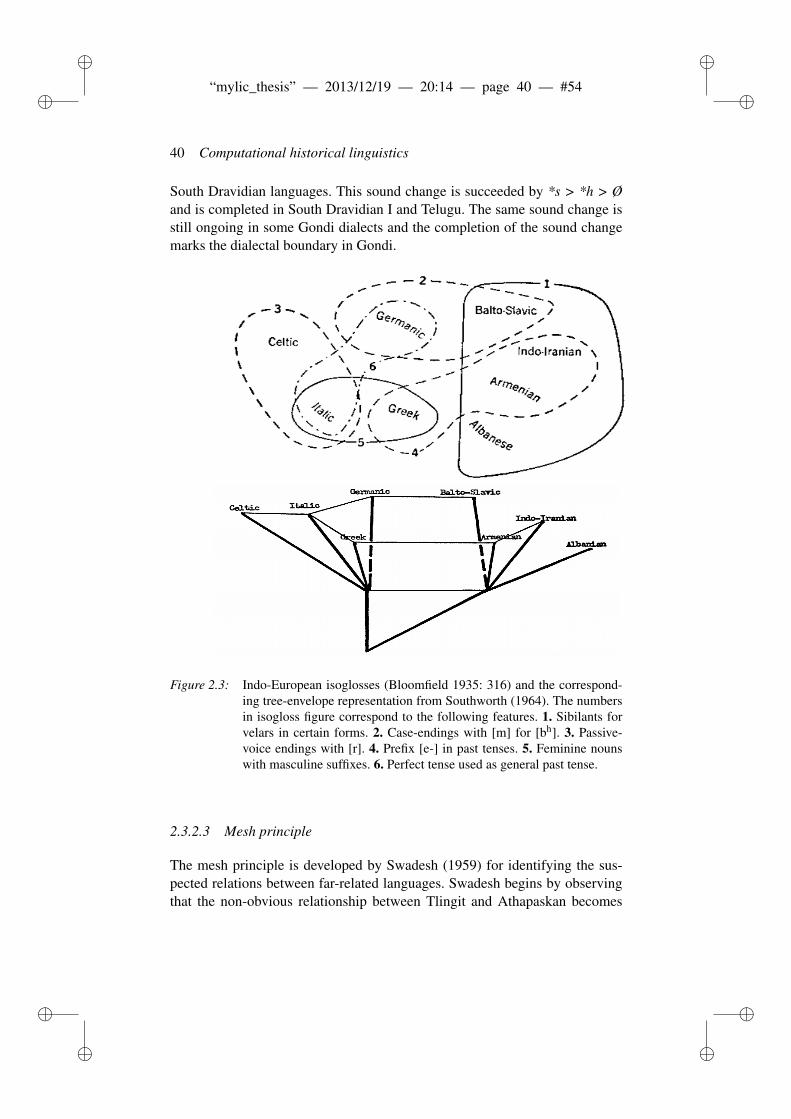
ii


ii

ii


South Dravidian languages. This sound change is succeeded by *s > *h > Øand is completed in South Dravidian I and Telugu. The same sound change isstill ongoing in some Gondi dialects and the completion of the sound changemarks the dialectal boundary in Gondi.

Figure 2.3: Indo-European isoglosses (Bloomfield 1935: 316) and the correspond-ing tree-envelope representation from Southworth (1964). The numbersin isogloss figure correspond to the following features. 1. Sibilants forvelars in certain forms. 2. Case-endings with [m] for [bh]. 3. Passive-voice endings with [r]. 4. Prefix [e-] in past tenses. 5. Feminine nounswith masculine suffixes. 6. Perfect tense used as general past tense.

2.3.2.3 Mesh principle

The mesh principle is developed by Swadesh (1959) for identifying the sus-pected relations between far-related languages. Swadesh begins by observingthat the non-obvious relationship between Tlingit and Athapaskan becomes

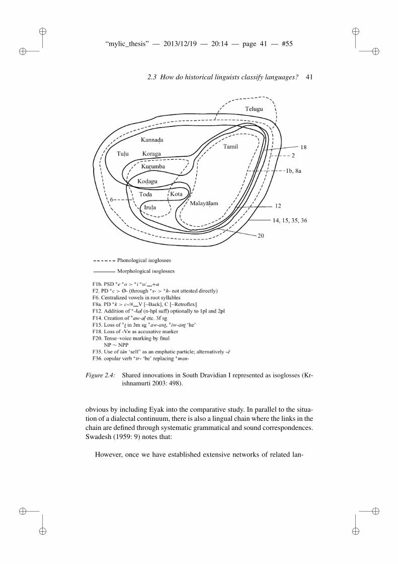
ii


ii

ii


Figure 2.4: Shared innovations in South Dravidian I represented as isoglosses (Kr-ishnamurti 2003: 498).

obvious by including Eyak into the comparative study. In parallel to the situa-tion of a dialectal continuum, there is also a lingual chain where the links in thechain are defined through systematic grammatical and sound correspondences.Swadesh (1959: 9) notes that:

However, once we have established extensive networks of related lan-

ii


ii

ii


guages connected with each other in a definite order of relative affinities,expressible, for example, in a two-dimensional diagram, it is possible totest each new language, as yet unplaced, at scattered points in the con-stellation to find where it comes the nearest to fitting.

This can be easily related to the Multi-dimensional Scaling technique (MDS;Kruskal 1964) which projects a multi-dimensional matrix to a two-dimensionalrepresentation. Consider the task of placing the position of a recalcitrant lan-guage in relation to other established subgroups, say Armenian. The first stepin this model will create a MDS diagram of IE languages without Armenianand then repeat the step with Armenian to see the shift in the positions of otherlanguages due to the introduction of Armenian. A much simpler case wouldbe to remove a pivotal language such as Sanskrit – that provided evidence forstress patterns in PIE (cf. Verner’s law) – to produce a MDS representation andthen repeat the step to see the shift of the languages in the fuller picture.

Given the recent application of biological network software to linguisticdata, Nichols and Warnow (2008) divide the mesh-like representations intotwo categories: implicit and explicit networks. Implicit networks do not showthe explicit interaction (such as borrowing and diffusion) between two inde-pendent languages such as French and English but show a mass of inheritedlinguistic material at the center of the network. The farther one gets away fromthe center and towards the branches of the network, the greater linguistic di-vergence one observes in the daughter languages. An example of such a net-work drawn from the cognate data of the Dravidian Etymological Dictionary(Burrow and Emeneau 1984) is given in figure 2.5. Explicit networks showthe contact scenario between the different branches in a family tree and areinferred from the three kinds of evidence (Nakleh, Ringe and Warnow 2005).

2.3.2.4 The comparative method as an iterative technique

The comparative method as explained in the previous section is iterative in na-ture. The flowchart presented in figure 2.1 captures the iterative aspect of thecomparative method. In the initial stages, the method accumulates evidencefrom basic vocabulary comparison and either reinforces or weeds out putativedaughter languages from comparison. Just as sound change that is character-ized to affect the suitable parts of vocabulary so does the comparative methodadds more evidence to it as it scans through more linguistic material. The ini-tial set of languages is always based on diagnostic evidence and not groundedin solid evidence. As Nichols (1996) notes, some branches of Indo-Europeansuch as Slavic were always known to be related due to the medieval records

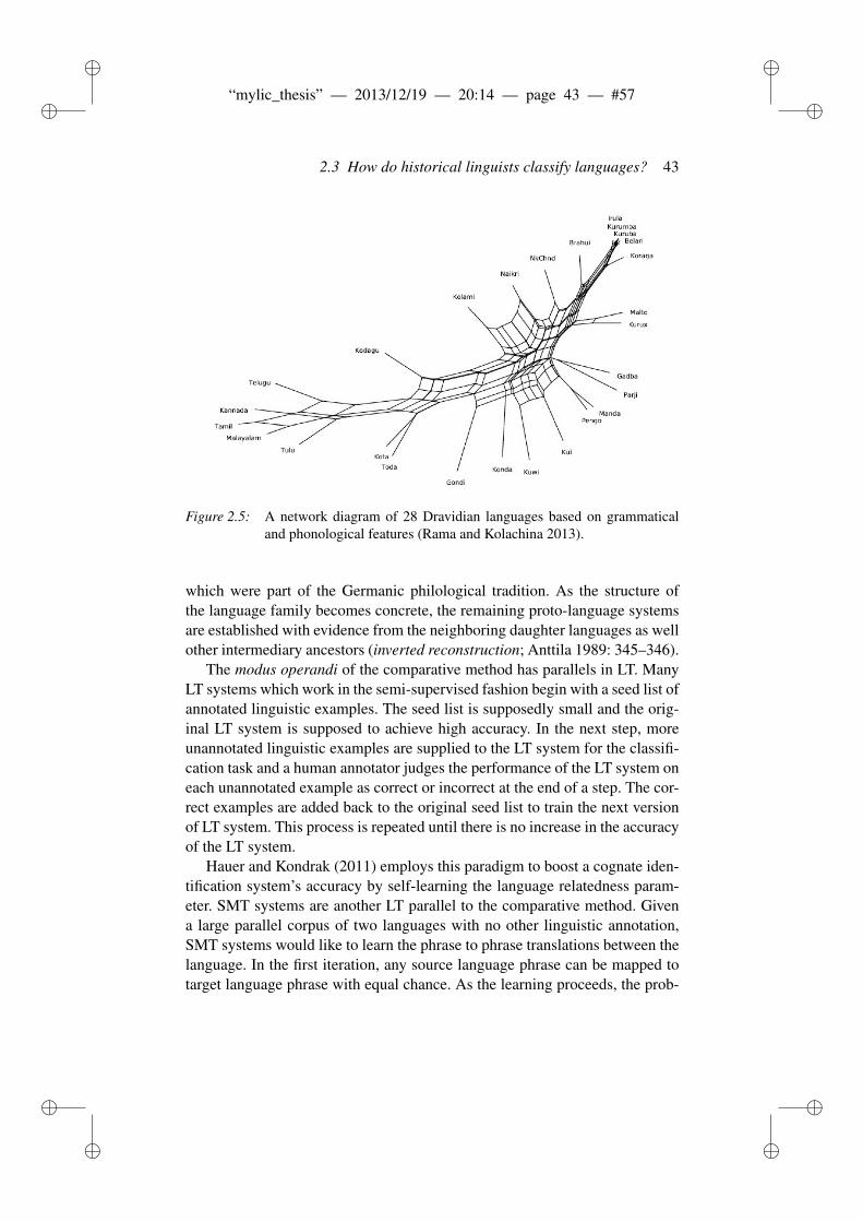
ii


ii

ii


Figure 2.5: A network diagram of 28 Dravidian languages based on grammaticaland phonological features (Rama and Kolachina 2013).

which were part of the Germanic philological tradition. As the structure ofthe language family becomes concrete, the remaining proto-language systemsare established with evidence from the neighboring daughter languages as wellother intermediary ancestors (inverted reconstruction; Anttila 1989: 345–346).

The modus operandi of the comparative method has parallels in LT. ManyLT systems which work in the semi-supervised fashion begin with a seed list ofannotated linguistic examples. The seed list is supposedly small and the orig-inal LT system is supposed to achieve high accuracy. In the next step, moreunannotated linguistic examples are supplied to the LT system for the classifi-cation task and a human annotator judges the performance of the LT system oneach unannotated example as correct or incorrect at the end of a step. The cor-rect examples are added back to the original seed list to train the next versionof LT system. This process is repeated until there is no increase in the accuracyof the LT system.

Hauer and Kondrak (2011) employs this paradigm to boost a cognate iden-tification system’s accuracy by self-learning the language relatedness param-eter. SMT systems are another LT parallel to the comparative method. Givena large parallel corpus of two languages with no other linguistic annotation,SMT systems would like to learn the phrase to phrase translations between thelanguage. In the first iteration, any source language phrase can be mapped totarget language phrase with equal chance. As the learning proceeds, the prob-

ii


ii

ii


abilities (evidence) for the source-target maps change and reach a local opti-mum where the evidence does not change over iterations. In a similar fashion,as evidence for language relationship accumulates, the comparative method’searlier predictions are subjected to change.

Bouchard-Côté et al. (2013) reconstruct Proto-Austronesian lexemes fromthe 200-word Swadesh list of 659 Austronesian languages. They assumed thetree topology of Austronesian language family as given and then proceededto reconstruct the proto-word forms of the 200 meanings. It has to be notedthat their method does not come close to the comparative method as the treestructure is given by linguists and not inferred from the data. Unfortunately,these authors reduce the reconstruction step to a search procedure over a treetopology inferred from the comparative method. Hence, there is an inherentcircularity in their method.

2.4 Alternative techniques in language classification

The standard historical linguistics textbooks list lexicostatistics and glotto-chronology as the alternative techniques in language classification. Howevernone of them note that positing genetic proximity based on cognate countsand the counts of shared phonological and grammatical innovations precededlexicostatistics. This crucial point is noted by Swadesh (1959) where Kroeberin 1907 used the established innovations to draw a two-dimensional proximitymaps for Californian languages. Campbell (2004) also makes the point thatonly a shared innovation can be used to classify languages. This brings us toan important question if there can be any method other than the comparativemethod to establish subgroups or classify languages. The rest of the section ison lexicostatistics and the recent classification methods that are beyond lexico-statistics. According to Wichmann (2013a), the textbooks usually portray theother methods as discredited.

2.4.1 Lexicostatistics

The lexicostatistical technique as introduced by Swadesh (1950) works onstandardized multi-lingual word lists. In contrary to the popular conceptionthat the similarities between two word lists are based on look-alikes, two wordsare judged to be similar if and only if they are cognates. The meanings in theselists are supposed to be resistant to borrowing and internal lexical replacement.The important question is how did Swadesh arrive at such a list? The multiplefamilies studied in CHL show that the list is actually robust and the classifica-

ii


ii

ii

2.4 Alternative techniques in language classification 45

tions inferred from the standardized word lists come close to the classificationsproposed through the comparative method (Greenhill and Gray 2009; Wich-mann et al. 2010a).

The issue of origin is investigated by Tadmor, Haspelmath and Taylor (2010).The authors quote from Swadesh (1971: 19) about the creation and refinementprocess from 215-word list to 100-word list.

In counting and statistics, it is convenient to operate with representativesamples, that is, a portion of the entire mass of facts so selected as toreflect the essential facts. For our lexical measure of linguistic diver-gence we need some kind of selected word list, a list of words for whichequivalents are found in each language or language variant [. . . ]

Apart from using the word lists for glottochronological studies, Swadesh in-tended to make the 100-word list a diagnostic vocabulary for investigatingknown as well as suspected language relationships.

2.4.2 Beyond lexicostatistics

A large amount of research has been conducted based on the 100/200 -wordlists. The availability of plug-and-play biological software spurred researchersto apply the methods to the Swadesh word lists to yield family trees basedon distance-based methods as well as character-based methods. An excerpt ofsuch input data is given in tables 2.4 and 2.5.

Items Danish Swedish Dutch English

‘person’ menneske/1 människa/1 mens/1 person/2‘skin’ skind/1 skinn/1, hud/2 huid/2 skin/1

Table 2.4: Two lexical characters for four Germanic languages (Wichmann 2010a:77–78). Each cell corresponds to a word form in a language and its cog-nacy state. word forms with the same state are cognates.

• Distance-based methods. The pair-wise cognate judgments are codedas sequence of ‘1’s and ‘0’s (cf. table 2.5) and the difference betweenthe character sequences is fed to a distance based algorithm. Some pop-ularly used distance-based algorithms are Neighbor-Joining (NJ), Un-weighted Pair Group Method with Arithmetic Mean (UPGMA), Fitch-Margoliash, and FastME (Fast Minimum Evolution). All the distancemethods try to optimize a criteria such as sum of the branches on the tree

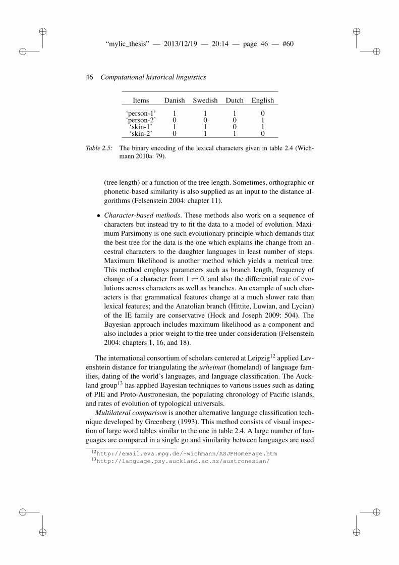
ii


ii

ii


Items Danish Swedish Dutch English

‘person-1’ 1 1 1 0‘person-2’ 0 0 0 1‘skin-1’ 1 1 0 1‘skin-2’ 0 1 1 0

Table 2.5: The binary encoding of the lexical characters given in table 2.4 (Wich-mann 2010a: 79).

(tree length) or a function of the tree length. Sometimes, orthographic orphonetic-based similarity is also supplied as an input to the distance al-gorithms (Felsenstein 2004: chapter 11).

• Character-based methods. These methods also work on a sequence ofcharacters but instead try to fit the data to a model of evolution. Maxi-mum Parsimony is one such evolutionary principle which demands thatthe best tree for the data is the one which explains the change from an-cestral characters to the daughter languages in least number of steps.Maximum likelihood is another method which yields a metrical tree.This method employs parameters such as branch length, frequency ofchange of a character from 1 0, and also the differential rate of evo-lutions across characters as well as branches. An example of such char-acters is that grammatical features change at a much slower rate thanlexical features; and the Anatolian branch (Hittite, Luwian, and Lycian)of the IE family are conservative (Hock and Joseph 2009: 504). TheBayesian approach includes maximum likelihood as a component andalso includes a prior weight to the tree under consideration (Felsenstein2004: chapters 1, 16, and 18).

The international consortium of scholars centered at Leipzig12 applied Lev-enshtein distance for triangulating the urheimat (homeland) of language fam-ilies, dating of the world’s languages, and language classification. The Auck-land group13 has applied Bayesian techniques to various issues such as datingof PIE and Proto-Austronesian, the populating chronology of Pacific islands,and rates of evolution of typological universals.

Multilateral comparison is another alternative language classification tech-nique developed by Greenberg (1993). This method consists of visual inspec-tion of large word tables similar to the one in table 2.4. A large number of lan-guages are compared in a single go and similarity between languages are used

12http://email.eva.mpg.de/~wichmann/ASJPHomePage.htm13http://language.psy.auckland.ac.nz/austronesian/

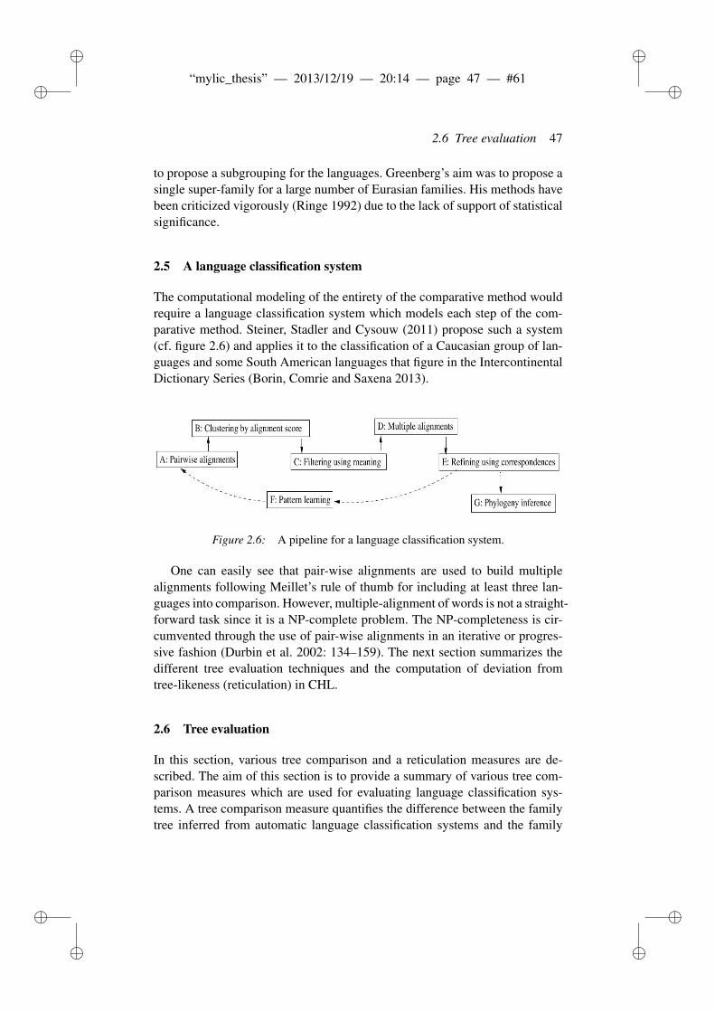
ii


ii

ii

2.6 Tree evaluation 47

to propose a subgrouping for the languages. Greenberg’s aim was to propose asingle super-family for a large number of Eurasian families. His methods havebeen criticized vigorously (Ringe 1992) due to the lack of support of statisticalsignificance.

2.5 A language classification system

The computational modeling of the entirety of the comparative method wouldrequire a language classification system which models each step of the com-parative method. Steiner, Stadler and Cysouw (2011) propose such a system(cf. figure 2.6) and applies it to the classification of a Caucasian group of lan-guages and some South American languages that figure in the IntercontinentalDictionary Series (Borin, Comrie and Saxena 2013).

Figure 2.6: A pipeline for a language classification system.

One can easily see that pair-wise alignments are used to build multiplealignments following Meillet’s rule of thumb for including at least three lan-guages into comparison. However, multiple-alignment of words is not a straight-forward task since it is a NP-complete problem. The NP-completeness is cir-cumvented through the use of pair-wise alignments in an iterative or progres-sive fashion (Durbin et al. 2002: 134–159). The next section summarizes thedifferent tree evaluation techniques and the computation of deviation fromtree-likeness (reticulation) in CHL.

2.6 Tree evaluation

In this section, various tree comparison and a reticulation measures are de-scribed. The aim of this section is to provide a summary of various tree com-parison measures which are used for evaluating language classification sys-tems. A tree comparison measure quantifies the difference between the familytree inferred from automatic language classification systems and the family

ii


ii

ii


tree inferred from the comparative method. This section also provides a de-scription of a reticulation measure called δ . The comparative method assumesthat languages diverge in a step-by-step fashion yielding a tree. However, itis widely known that language evolution is not always tree-like. For instance,English has borrowed French vocabulary but is still a Germanic language dueto its descent from Proto-Germanic. As noted previously, a network model isa graphical device of the amount of deviation of tree-likeness. But it does notprovide a number for the amount of deviation. The δ measure fills in this gapand provides a score for deviation from tree-likeness. The four different treecomparison techniques and δ are described in the next section.

2.6.1 Tree comparison measures

Robinson-Foulds (RF) Distance. The RF distance is defined as the number ofdissimilar bipartitions between an inferred tree and gold-standard tree. A bi-partition is a pair of language sets resulting from the removal of a internal edgein a phylogenetic tree. For a phylogenetic tree with N languages, there are atmost N−3 bipartitions. Thus, the RF distance measures the dissimilarity in thetopology between the inferred tree and the corresponding family tree. It shouldbe noted that the RF distance does not take branch lengths into account. Anytree inference algorithm yields a phylogenetic tree with branch lengths. RFdistance throws away the branch length information when comparing the in-ferred tree with the family tree. Steel and Penny (1993) introduced three othermeasures as alternatives to RF distance. Each of these measures are describedin detail below.

Branch Score Difference (BSD). BSD is related to RF and takes into accountbranch lengths. Instead of computing the number of dissimilar partitions be-tween the inferred tree and family tree, BSD computes the sum of the absolutedifference in each of the internal branch lengths in the two trees. If an internalbranch is absent in one tree and present in the other tree then the branch lengthfor the absent branch is treated as zero.

Path Length Distance (PD). This measure is based on the idea that thedistance between two languages can be expressed as the number of edges(branches) in the shortest path (in the tree) connecting the two languages. Eachcell of a path length matrix (PDM) consists of the path length between a pairof languages in a phylogenetic tree. PD is computed as the square root of theaverage of the square of the difference between each cell of the PDM of theinferred tree and the corresponding cell in the PDM of the linguistic tree.

Weighted Path Length Distance (WPD). WPD is computed in a similar fash-ion to that of PD except that the path length for a pair of languages, is computed

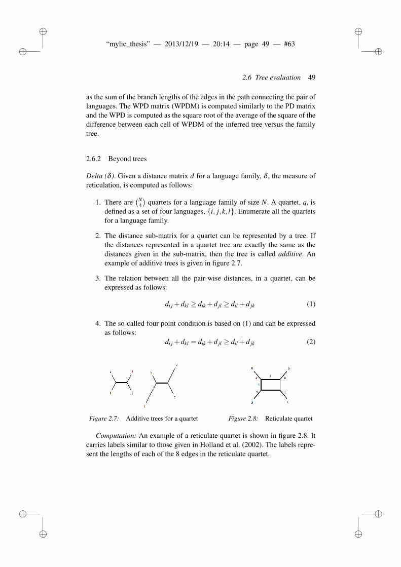
ii


ii

ii

2.6 Tree evaluation 49

as the sum of the branch lengths of the edges in the path connecting the pair oflanguages. The WPD matrix (WPDM) is computed similarly to the PD matrixand the WPD is computed as the square root of the average of the square of thedifference between each cell of WPDM of the inferred tree versus the familytree.

2.6.2 Beyond trees

Delta (δ ). Given a distance matrix d for a language family, δ , the measure ofreticulation, is computed as follows:

1. There are(N

4

)quartets for a language family of size N. A quartet, q, is

defined as a set of four languages, {i, j,k, l}. Enumerate all the quartetsfor a language family.

2. The distance sub-matrix for a quartet can be represented by a tree. Ifthe distances represented in a quartet tree are exactly the same as thedistances given in the sub-matrix, then the tree is called additive. Anexample of additive trees is given in figure 2.7.

3. The relation between all the pair-wise distances, in a quartet, can beexpressed as follows:

di j +dkl ≥ dik +d jl ≥ dil +d jk (1)

4. The so-called four point condition is based on (1) and can be expressedas follows:

di j +dkl = dik +d jl ≥ dil +d jk (2)

Figure 2.7: Additive trees for a quartet Figure 2.8: Reticulate quartet

Computation: An example of a reticulate quartet is shown in figure 2.8. Itcarries labels similar to those given in Holland et al. (2002). The labels repre-sent the lengths of each of the 8 edges in the reticulate quartet.

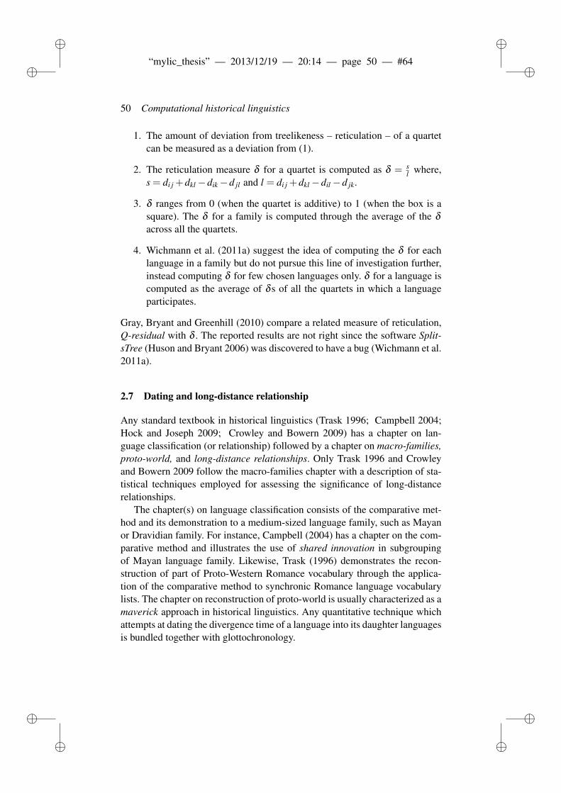
ii


ii

ii


1. The amount of deviation from treelikeness – reticulation – of a quartetcan be measured as a deviation from (1).

2. The reticulation measure δ for a quartet is computed as δ = sl where,

s = di j +dkl−dik−d jl and l = di j +dkl−dil−d jk.

3. δ ranges from 0 (when the quartet is additive) to 1 (when the box is asquare). The δ for a family is computed through the average of the δ

across all the quartets.

4. Wichmann et al. (2011a) suggest the idea of computing the δ for eachlanguage in a family but do not pursue this line of investigation further,instead computing δ for few chosen languages only. δ for a language iscomputed as the average of δ s of all the quartets in which a languageparticipates.

Gray, Bryant and Greenhill (2010) compare a related measure of reticulation,Q-residual with δ . The reported results are not right since the software Split-sTree (Huson and Bryant 2006) was discovered to have a bug (Wichmann et al.2011a).

2.7 Dating and long-distance relationship

Any standard textbook in historical linguistics (Trask 1996; Campbell 2004;Hock and Joseph 2009; Crowley and Bowern 2009) has a chapter on lan-guage classification (or relationship) followed by a chapter on macro-families,proto-world, and long-distance relationships. Only Trask 1996 and Crowleyand Bowern 2009 follow the macro-families chapter with a description of sta-tistical techniques employed for assessing the significance of long-distancerelationships.

The chapter(s) on language classification consists of the comparative met-hod and its demonstration to a medium-sized language family, such as Mayanor Dravidian family. For instance, Campbell (2004) has a chapter on the com-parative method and illustrates the use of shared innovation in subgroupingof Mayan language family. Likewise, Trask (1996) demonstrates the recon-struction of part of Proto-Western Romance vocabulary through the applica-tion of the comparative method to synchronic Romance language vocabularylists. The chapter on reconstruction of proto-world is usually characterized as amaverick approach in historical linguistics. Any quantitative technique whichattempts at dating the divergence time of a language into its daughter languagesis bundled together with glottochronology.

ii


ii

ii

2.7 Dating and long-distance relationship 51

Interestingly, Campbell (2004) uses the terms glottochronology and lexico-statistics interchangeably. Although both the methods use the same datasets,their object of investigation is different. It has to be kept in mind that lexico-statistics is concerned with subgrouping whereas glottochronology provides adivergence date to a pair of languages. The merits and demerits of the quan-tification of time depth in historical linguistics is addressed in a collection ofarticles edited by Renfrew, McMahon and Trask (2000). The main criticismagainst glottochronology is that the method works with a constant rate of lex-ical replacement (in general, language change). However, the recent phyloge-netic techniques (cf. section 2.4.2) do not necessarily assume a constant rate oflanguage change. Hence, the trees inferred from modern methods can be datedusing much sophisticated statistical techniques (Gray and Atkinson 2003).Even McMahon and McMahon 2005, who employ the latest computationaltechniques from computational biology to classify languages from Andes toIndo-Aryan languages (McMahon and McMahon 2007) spoken in NorthernIndia refrain from assigning dates to splits (McMahon and McMahon 2005:177).

Given that there is such a huge criticism against the aforementioned tech-niques, how come there are so many posited families? Is the comparativemethod highly successful in positing these families? Unfortunately, the answeris no. There are only few language families which are posited by the compar-ative method. For instance, consider the languages spoken in New Guinea.There are more than 800 languages spoken in the small island which do notbelong to Austronesian language family. How are these languages classified?In fact, the recent textbook of Hock and Joseph 2009: 445–454 does not listany of New Guinea’s languages. Interestingly, many of the proposed languagefamilies in New Guinea are proposed based on cognate counts, similarities inpronouns, typological similarity or geographical similarity (Wichmann 2013b:originally from Foley 1986). The situation for South American languages isonly a little better (Hammarström 2013), with many well established families,but also many relations that remain to be worked out using the comparativemethod (cf. Campbell 2012 for progress in this regard).

Long-distance genetic proposals is a contentious topic in historical linguis-tics. Probabilistic testing of suspected long-distance relationships or linguistichypotheses is met with skepticism. In a survey, Kessler (2008: 829; my em-phasis) makes the following observation:

Probabilistic analysis and the language modeling it entails are worthytopics of research, but linguists have rightfully been wary of claims oflanguage relatedness that are based primarily on probabilities. If nothingelse, skepticism is aroused when one is informed that a potential long-

ii


ii

ii


range relationship whose validity is unclear to experts suddenly becomesa trillion-to-one sure bet when a few equations are brought to bear onthe task.

Examples of such probabilistic support from Kessler 2008: 828:

• Nichols (1996) demonstrates that any language with an Indo-Europeangender system would be, in fact, Indo-European. She did this by count-ing frequencies of languages that have genders, that a language shouldhave at least three genders, that one of the gender markers should be-s, and so on from a large number of languages. The final number forchance similarity is .57× 10−6 which is such a small number that theoriginal hypothesis cannot be ruled out as a case of chance similarity.

• Dolgopolsky (1986) found similarities between words for 13 conceptsand ruled out the chance similarity with a numerical support of 10−20.The small number provides support for a broad Sibero-European lan-guage family.

Summarizing, any attempt at comparing the proto-languages of even spa-tially proximal families is usually viewed with suspicion. The next subsectiondiscusses the reality of linguistic reconstruction and attempts at correlating thelinguistic evidence with archaeological and other kinds of evidence.

2.7.1 Non-quantitative methods in linguistic paleontology

Linguistic paleontology makes inferences on the culture, society, and ecologyof prehistoric peoples based on reconstructed linguistic evidence (Hock andJoseph 2009: 481). Linguistic paleontology opens a window into the differ-ent aspects of life of prehistoric populations. Borrowed words correspondingto a technical innovation, names of places, and names of people allow his-torical linguists to assign a date to important linguistic changes affecting apre-language. Migration histories also provide evidence for the split of thecurrent languages from their ancestor. For instance, the vocabulary reconstruc-tions of domesticated animals in PIE are taken to indicate that the PIE speakerswere food-producers. The appearance of loan words and the subsequent soundchanges they triggered, also allow historical linguists to assign a date to thesound change. For instance, looking into the Romani vocabulary and tracingthe sources of loans provides information on the pattern of migration of Ro-mani people into Europe.

ii


ii

ii

2.7 Dating and long-distance relationship 53

Locating the probable geographical source of proto-language speakers isa highly debated topic. Historical evidence shows that the migrations of Ger-manic speakers caused the split of the Germanic ancestral language and thisoccurred about 2100 BP (before present). This date is considered as the an-tiquity of Proto-Germanic. The split date of Slavic languages is given around1500 BP since the written records of sixth century describe the state of politi-cal affairs and geographic expansion of the Common Slavic language (Holmanet al. 2011). The skepticism regarding the search for putative homelands canbe summarized in the following quote of Mallory (1989: 143).

the quest for the origins of the Indo-Europeans has all the fascinationof an electric light in the open air on a summer night: it tends to attractevery species of scholar or would-be savant who can take pen to hand

Sapir (1916) proposes a model for locating proto-language homelands call-ed the centre of gravity model. Under this model, the homeland of a languagefamily is the region that shows the highest amount of linguistic diversity. Thehomeland for a language family has the highest amount of divergence in termsof languages belonging to the oldest branches of the family since this pointcorresponds to the initial divergence of the language family.

The questions of dating, finding homelands, and evolution of cultural traitshad been addressed from a computational perspective in recent years. A fewexamples of such research are:

• Holden (2002) applies maximum parsimony to show that the Bantu fam-ily’s language trees reflect the spread of farming in sub-Saharan Africa.

• Jordan et al. (2009) apply Bayesian techniques to study the evolutionof matrilocal residence from Proto-Austronesian. This is done by ex-amining the evolution of matrilocal traits in the different Austronesianlanguages.

• Wichmann, Müller and Velupillai (2010) implement Sapir’s idea, find-ing the area of greatest diversity based on lexical evidence and identifythat area with the homeland; the approach is applied across the world’slanguage families.

• Walker et al. (2012) apply Bayesian techniques to study the cultural evo-lution in the Tupian language family in Lowland South America.

• Bouckaert et al. (2012) apply Bayesian techniques to map the originsand expansions of the Indo-European language family.

ii


ii

ii


In conclusion, a combination of computational, statistical, linguistic, andanthropological techniques can help address some questions about the originand spread of language families both spatially and temporally.

2.8 Conclusion

This chapter presented a linguistic introduction to the processes of linguisticchange, models of language evolution, computational modeling of the linguis-tic changes, and the recent developments in computational historical linguis-tics. The next chapter will summarize the various linguistic databases that re-sulted from digitization as well as new efforts to augment the older vocabularyand typological databases.

ii


ii

ii

3 DATABASES

This chapter describes the various linguistic databases used for language clas-sification. The papers listed in the second part of the thesis describe the Au-tomated Similarity Judgment Program (ASJP) database, World Atlas of Lan-guage Structures (WALS) database, and the Europarl parallel corpora (fromEuropean parliamentary proceedings). Thus, this chapter will focus on lin-guistic databases which are not listed in part II of the thesis. The linguisticdatabases used in language classification can be classified into the followingthree types.

• Cognate databases. Linguistic databases that show the state of phono-logical, lexical, and grammatical features (characters) across a languagefamily. Core vocabulary databases with or without cognate judgments.

• Typological databases presenting the variation of a typological featureon a graded scale.

• There are other linguistic databases that show linguistic features such asphoneme inventory size and part-of-speech annotation.

3.1 Cognate databases

Core vocabulary databases are parallel word lists for a language group. Thesize of the word lists usually range from 40–215 in these databases. The basicvocabulary databases are lexical in nature and may also carry cognate judg-ments. The core vocabulary databases can be used for lexicostatistical studiesand also as an input to the distance-based or character-based phylogenetic al-gorithms (cf. section 2.4.2).

ii


ii

ii

56 Databases

3.1.1 Dyen’s Indo-European database

Dyen, Kruskal and Black (1992) prepared a lexicostatistical database of 95Indo-European speech varieties for 200 concepts. The database has word formsand cognate judgments for the Celtic, Germanic, Indo-Iranian, Baltic, Slavic,Greek, Armenian, and Albanian branches of IE. The word forms in the databaseare not phonetically transcribed and hence, are not fit for phonetic analysis orcomputing phonetic similarity distances between the speech varieties. How-ever, the database was used for the purposes of cognate identification and in-ference of a Levenshtein-distance based IE tree (Ellison and Kirby 2006).

3.1.2 Ancient Indo-European database

Ringe, Warnow and Taylor (2002) designed a database consisting of IE wordlists for 24 ancient Indo-European languages. The database has 120 conceptsin addition to the 200 Swadesh concepts, 15 morphological characters, and22 phonological characters. Each character can exhibit multiple states. Thepresence of the ruki rule – change of PIE */s/ to */š/ before */r/, */u/, */k/,or */i/ – is coded as 2 in Indo-Iranian and Balto-Slavic languages and its ab-sence as 1 in other IE languages. Whenever a meaning has two forms, eachform is coded as a separate character and the cognate judgments are assignedaccordingly. For instance, Luvian shows two word forms for the concept ‘all(plural)’. Each word form is cognate with word forms present in some otherIE languages. Thus, the two word forms are listed as separated characters.Nakhleh et al. (2005) compare the performance of various distance-based andcharacter-based algorithms on this dataset.

3.1.3 Intercontinental Dictionary Series (IDS)

IDS is an international collaborative lexical database for non-prestigious andlittle known languages. The database is organized into 23 chapters consistingof 1,310 concepts. The database has a large collection of languages from SouthAmerica and the Caucasus region. The database has 215 word lists which areavailable for online browsing and download (Borin, Comrie and Saxena 2013).An extended concept list is proposed in the Loanword Typology Project (LWT)described in the next section. Cysouw and Jung (2007) use the IDS word listsfrom English, French, and Hunzib for cognate identification through multi-

ii


ii

ii

3.1 Cognate databases 57

gram alignments.14

3.1.4 World loanword database

The World Loanword Database, under the auspices of LWT, is a collabora-tive database edited by Haspelmath and Tadmor (2009a). This database is anextension of the concept lists proposed in the IDS project. The meanings are or-ganized into 24 semantic fields. For each concept, the database contains wordforms, the gloss of a word form, the source of the borrowing (if it is a bor-rowing) and the expert’s confidence on the borrowing on a scale of 1–5, andthe age of the word for 41 languages. The age of the word is the time of theearliest attestation or reconstruction for a non-borrowed word; for a borrowedword, age is the time period in which the word was borrowed. Tadmor, Haspel-math and Taylor (2010) apply the criteria such as (a) fewest borrowed coun-terparts (borrowability), (b) representation (fewest word forms for a meaningin a language), (c) analyzability (for a multi-word expression), (d) age to ar-rive at a 100-word list called the Leipzig-Jakarta list. The 100-word Leipzig-Jakarta concept list has 60 concepts in common with the 100-word Swadeshlist. Holman et al. (2008a) develop a ranking procedure to rank the meanings ofthe 100-word Swadesh list according to lexical stability and correlate stabilityranks and borrowability scores from the still unpublished results of the LWT,finding the absence of a correlation, suggesting, importantly, that borrowabilityis not a major contributor to lexical stability.

3.1.5 List’s database

List and Moran (2013) developed an python-based open-source toolkit forCHL. This toolkit implements the pipeline described in chapter 2 (cf. fig-ure 2.6). The authors also provide a manually curated 200-word Swadesh listfor the Germanic and Uralic families, Japanese and Chinese dialects. The wordlists are encoded in IPA and the toolkit provides libraries for automatic con-version from IPA to coarser phonetic representations such as ASJP and Dolgo-polsky’s sound classes.

14A n-gram of length i in language A is mapped to a n-gram of length j in language B where1≤ i, j ≤ n.

ii


ii

ii

58 Databases

3.1.6 Austronesian Basic Vocabulary Database (ABVD)

ABVD15 (Greenhill, Blust and Gray 2008) is a vocabulary database for 998Austronesian languages. The database has 203,845 lexical items for the Swad-esh concept list (of length 210). The database has cognate judgments and hasbeen widely used for addressing a wide-range of problems in Austronesianhistorical linguistics (Greenhill and Gray 2009).

3.2 Typological databases

3.2.1 Syntactic Structures of the World’s Languages

Syntactic Structures of the World’s Languages (SSWL)16 is a collaborative,typological database of syntactic structures for 214 languages. Although thedata is available for download, not much is known about the current state of itsdevelopment.

3.2.2 Jazyki Mira

Jazyki Mira is a typological database which is very much like WALS but withfuller coverage for a smaller set of Eurasian languages (Polyakov et al. 2009).Polyakov et al. (2009) compare the calculations of typological similarity andtemporal stability of language features from the data obtained from WALS andJazyki Mira.

3.2.3 AUTOTYP

AUTOTYP (Autotypology) is another typological database based at the Uni-versity of Zurich (Bickel 2002). Rather than working with pre-defined list oftypological features, the project modifies the list of typological features asmore languages enter into the database. The database was used for investi-gating quantitative and qualitative typological universals (Bickel and Nichols2002).

15Accessed on 2nd December 2013.16http://sswl.railsplayground.net/

ii


ii

ii

3.3 Other comparative linguistic databases 59

3.3 Other comparative linguistic databases

There are some databases which are indirectly related to CHL but so far havenot been employed for language classification.

3.3.1 ODIN

Online Database of Interlinear Text (ODIN; Lewis and Xia 2010) is an au-tomatically extracted database from scholarly documents present on the web.The database has more than 190,000 instances of interlinear text for more than1,000 languages. The database provides search facilities for searching the lan-guage data and the source of the data. The database is available for download.The authors parse the English gloss text and project the syntactic structuresto the original language data creating a parallel treebank in the process. Thedatabase also allows search by syntactic trees and categories.

3.3.2 PHOIBLE

PHOnetics Information Base and LExicon (PHOIBLE)17 is a phonological andtypological database for more than 600 languages. The database has phone-mic and allophonic inventories, and the conditioning environments that are ex-tracted from secondary sources like grammars and other phonological databas-es (Moran 2012).

3.3.3 World phonotactic database

The World phonotactic database has been recently published by a group of re-searchers at the Australian National University (Donohue et al. 2013). Thedatabase contains phonotactic information for more than 2,000 languages,and segmental data for an additional 1,700 languages. The main focus of thisdatabase is on the languages of the Pacific region.

3.3.4 WOLEX

The World Lexicon of Corpus is a database of lexicons extracted from gram-mars and corpora for 47 languages by Graff et al. (2011). The website18 lists

17Accessed http://phoible.org/ on 2nd December 2013.18http://qrlg.blogspot.se/p/wolex.html

ii


ii

ii

60 Databases

the 47 languages, size of lexicon, and the source of data. Nothing much isknown about the methodology and development of the corpus from the web-site of the project.

3.4 Conclusion

In this chapter, various linguistic databases are summarized. Not all of thedatabases have been used for language classification. As noted by Borin, Com-rie and Saxena (2013), using larger word lists (such as IDS) would be useful ininvestigating the rarer linguistic phenomena since the data requirement growon an exponential scale (Zipf’s law). To the best of our knowledge, except forthe Ancient languages IE database and ABVD, the rest of the databases havenot been exploited to their fullest for comparative linguistic investigations.

ii


ii

ii

4 SUMMARY AND FUTURE

WORK

This chapter summarizes the work reported in the thesis and provides pointersto future work.

4.1 Summary

Chapter 1 places the work in part II in the context of LT and gives relatedwork in CHL. Further, the chapter gives an introduction to some problems andmethods in traditional historical linguistics.

Chapter 2 introduces the concepts of linguistic diversity and differences,various linguistic changes and computational modeling of the respective chan-ges, the comparative method, tree inference and evaluation techniques, andlong-distance relationships.

Chapter 3 describes various historical and typological databases releasedover the last few years.

The following papers have as their main theme the application of LT tech-niques to address some of the classical problems in historical linguistics. Thepapers Rama and Borin 2013, Rama 2013, and Rama and Borin 2014 workwith standardized vocabulary lists whereas Rama and Borin 2011 works withautomatically extracted translational equivalents for 55 language pairs. Most ofthe work is carried out on the ASJP database, since the database has been cre-ated and revised with the aim of maximal coverage of the world’s languages.This does not mean that the methods will not work for larger word lists suchas IDS or LWT.

Rama 2013 provides a methodology on automatic dating of the world’slanguages using phonotactic diversity as a measure of language divergence.Unlike the glottochronological approaches, the explicit statistical modelingof time splits (Evans, Ringe and Warnow 2006), and the use of Levenshteindistance for dating of the world’s languages (Holman et al. 2011), the paperemploys the type count of phoneme n-grams as a measure of linguistic diver-gence. The idea behind this approach is that the language group showing the

ii


ii

ii

62 Summary and future work

highest phonotactic diversity is also the oldest. The paper uses generalized lin-ear models (with the log function as link, known as Γ regression) to model thedependency of the calibration dates with the respective n-grams. This modelovercomes the standard criticism of “assumption of constant rate of languagechange” and each language group is assumed to have a different rate of evolu-tion over time. This paper is the first attempt to apply phonotactic diversity asa measure of linguistic divergence.

The n-gram string similarity measures applied in Rama and Borin 2014show that n-gram measures are good at internal classification whereas Lev-enshtein distance is good at discriminating related languages from unrelatedones. The chapter also introduces a multiple-testing procedure – False Dis-covery Rate – for ranking the performance of any number of string similaritymeasures. The multiple-testing procedure tests whether the differential perfor-mance of the similarity measures is statistically significant or not. This pro-cedure has already been applied to check the validity of suspected languagerelationships beyond the reach of the comparative method (Wichmann, Hol-man and List 2013).

Rama and Kolachina 2012 correlate typological distances with basic vocab-ulary distances, computed from ASJP, and find that the correlation – betweenlinguistic distances computed from two different sources – is not accidental.

Rama and Borin 2013 explores the application of n-gram measures to pro-vide a ranking of the 100-word list by its genealogically stability. We compareour ranking with the ranking of the same list by Holman et al. (2008a). We alsocompare our ranking with shorter lists – with 35 and 23 items – proposed byDolgopolsky (1986) and Starostin (1991: attributed to Yakhontov) for inferringlong-distance relationships. We find that n-grams can be used as a measure oflexical stability. This study shows that information-theoretic measures can beused in CHL (Raman and Patrick 1997; Wettig 2013).

Rama and Borin 2011 can be seen as the application of LT techniques forcorpus-based CHL. In contrast to the rest of papers which work with the ASJPdatabase, in this paper, we attempt to extract cognates and also infer a phenetictree for 11 European languages using three different string similarity measures.We try to find cognates from cross-linguistically aligned words by imposing asurface similarity cut-off.

4.2 Future work

The current work points towards the following directions of future work.

• Exploiting longer word lists such as IDS and LWT for addressing vari-ous problems in CHL.

ii


ii

ii

4.2 Future work 63

• Apply all the available string similarity measures and experiment withtheir combination for the development of a better language classificationsystem. To make the most out of short word lists, skip-grams can be usedas features to train linear classifiers (also string kernels; Lodhi et al.2002) for cognate identification and language classification.

• Combine typological distances with lexical distances and evaluate theirsuccess at discriminating languages. Another future direction is to checkthe relationship between reticulation and typological distances (Dono-hue 2012).

• Since morphological evidence and syntactic evidence are important forlanguage classification, the next step would be to use multilingual tree-banks for the comparison of word order, part-of-speech, and syntacticsubtree (or treelet) distributions (Kopotev et al. 2013; Wiersma, Ner-bonne and Lauttamus 2011).

• The language dating paper can be extended to include the phylogenetictree structure into the model. Currently, the prediction model assumesthat there is no structure between the languages of a language group. Amodel which incorporates the tree structure into the dating model wouldbe a next task (Pagel 1999).

• Application of the recently developed techniques from CHL to digi-tized grammatical descriptions of languages or public resources such asWikipedia and Wiktionary to build typological and phonological databa-ses (Nordhoff 2012) could be a task for the future.

ii


ii

ii

ii


ii

ii

Part II

Papers on application ofcomputational techniques to

vocabulary lists for automaticlanguage classification

ii


ii

ii

ii


ii

ii

5 ESTIMATING LANGUAGE

RELATIONSHIPS FROM A

PARALLEL CORPUS

Taraka Rama, Lars Borin 2011. Estimating Language Relationships from aParallel Corpus. A Study of the Europarl Corpus. NEALT Proceedings Series(NODALIDA 2011 Conference Proceedings). 161–167

Abstract

Since the 1950s, Linguists have been using short lists (40–200 items) of ba-sic vocabulary as the central component in a methodology which is claimedto make it possible to automatically calculate genetic relationships among lan-guages. In the last few years these methods have experienced something of arevival, in that more languages are involved, different distance measures aresystematically compared and evaluated, and methods from computational bi-ology are used for calculating language family trees. In this paper, we explorehow this methodology can be extended in another direction, by using largerword lists automatically extracted from a parallel corpus using word alignmentsoftware. We present preliminary results from using the Europarl parallel cor-pus in this way for estimating the distances between some languages in theIndo-European language family.

5.1 Introduction

Automatic identification of genetic relationships among languages has gainedattention in the last few years. Estimating the distance matrix between the lan-guages under comparison is the first step in this direction. Then a distancebased clustering algorithm can be used to construct the phylogenetic tree for afamily. The distance matrix can be computed in many ways. Lexical, syntacticand semantic features of the languages can be used for computing this ma-trix (Ringe, Warnow and Taylor 2002). Of these, lexical features are the mostwidely used features, most commonly in the form of Swadesh lists.

ii


ii

ii

68 Estimating language relationships from a parallel corpus

Swadesh lists are short lists (40–200 items) of basic senses which are sup-posed to be universal. Further, the words expressing these senses in a languageare supposed to be resistant to borrowing. If these two assumptions hold, itfollows that such lists can be used to calculate a numerical estimate of geneticdistances among related languages, an endeavor referred to as lexicostatistics.A third assumption which was often made in the older literature was that the re-placement rate of this basic vocabulary was constant and could be expressed asa constant percentage of the basic vocabulary being replaced over some unit oftime (exponential decay). This third assumption has generally been abandonedas flawed and with it the body of research that it motivated, often referred to asglottochronology.

In lexicostatistics, the similarity between two languages is the percentageof shared cognates between the two languages in such a list. In the terminol-ogy of historical linguistics, cognates are words across languages which havedescended independently in each language from the same word in a commonancestor language. Hence, loanwords are not cognates. Cognates are identifiedthrough regular sound correspondences. For example, English∼German night∼ Nacht ‘night’ and hound ∼Hund ‘dog’ are cognates. If the languages are farenough removed in time, so that sound changes have been extensive, it is oftenfar from obvious to the non-expert which words are cognates, e.g. English ∼Greek hound ∼ kuon ‘dog’ or English ∼ Armenian two ∼ erku ‘two’.

In older lexicostatistical work (e.g. Dyen, Kruskal and Black 1992), cog-nates are manually identified as such by experts, but in recent years there hasbeen a strong interest in developing automatic methods for cognate identifica-tion. The methods proposed so far are generally based on some form of ortho-graphic similarity19 and cannot distinguish between cognates on the one handand loanwords or chance resemblances on the other. Confusingly, the wordpairings or groups identified in this way are often called cognates in the com-putational linguistics literature, whereas the term correlates has been proposedin historical linguistics for the same thing (McMahon and McMahon 2005). Inany case, the identification of such orthographically similar words is a centralcomponent in any automatic procedure purporting to identify cognates in thenarrower sense of historical linguistics. Hence, below we will generally referto these methods as methods for the identification of cognates, even if theyactually in most cases identify correlates.

There have been numerous studies employing string similarity measuresfor the identification of cognates. The most commonly used measure is nor-

19Even though the similarity measures used in the literature all work with written representa-tions of words, these written representations are often in fact phonetic transcriptions, so that wecan say that we have a phonetic similarity measure. For this reason we will use “orthographic”and “phonetic” interchangeably below.

ii


ii

ii

5.2 Related work 69

malized edit distance. It is defined as the minimum number of deletions, sub-stitutions and insertions required to transform one string to another. There havealso been studies on employing identification of cognates using string similar-ity measures for the tasks of sentence alignment (Simard, Foster and Isabelle1993), statistical machine translation (Kondrak, Marcu and Knight 2003) andtranslational lexicon extraction (Koehn and Knight 2002).

The rest of this paper is structured as follows. Section 5.2 discusses relatedwork. Section 5.3 explains the motivation for using a parallel corpus and de-scribes the approach.

5.2 Related work

Kondrak (2002a) compares a number of algorithms based on phonetic and or-thographical similarity for judging the cognateness of a word pair. His worksurveys string similarity/ distance measures such as edit distance, Dice coeffi-cient and longest common subsequence ratio (LCSR) for the task of cognateidentification. The measures were tested on vocabulary lists for the Algonquianlanguage family and Dyen, Kruskal and Black (1992) Indo-European lists.

Many studies based on lexicostatistics and phylogenetic software have beenconducted using Swadesh lists for different language families. Among the no-table studies for Indo-European are the lexicostatistical experiments of Dyen,Kruskal and Black 1992 and the phylogeny experiments of Ringe, Warnow andTaylor 2002 and Gray and Atkinson 2003. In another study, Ellison and Kirby(2006) used intra-language lexical divergence for measuring the inter-languagedistances for the Indo-European language family.

Recently, a group of scholars (Wichmann et al. 2010a; Holman et al.2008a) have collected 40-item Swadesh word lists for about two thirds of theworld’s languages.20 This group uses a modified Levenshtein distance betweenthe lexical items as the measure of the inter-language distance.

Singh and Surana (2007) use corpus based measures for estimating the dis-tances between South Asian languages from noisy corpora of nine languages.They use a phonetics based similarity measure called computational phoneticmodel of scripts (CPMS; Singh, Surana and Gali 2007) for pruning the possi-ble cognate pairs between languages. The mean of the similarity between thepruned cognate pairs using this measure is estimated as the distance betweenthe languages.

20Their collaboration goes under the name of the Automated Similarity Judgement Program(ASJP) and their current dataset (in late 2010) contains word lists for 4,820 languages, whereall items are rendered in a coarse phonetic transcription, even for those languages where aconventional written form exists.

ii


ii

ii


Bergsma and Kondrak (2007) conduct experiments for cognate identifica-tion using alignment-based discriminative string similarity. They automaticallyextract cognate candidate pairs from the Europarl corpus (Koehn 2005) andfrom bilingual dictionaries for the language pairs English–French, English–German, English–Greek, English–Japanese, English–Russian, and English–Spanish. Bouchard-Côté et al. (2007) also use the Europarl corpus to extractcognates for the task of modeling the diachronic phonology of the Romancelanguages. In neither case is the goal of the authors to group the languagesgenetically by family, as in the work presented here. The previous work whichcomes closest to the work presented here is that of Koehn 2005, who trainspair-wise statistical translation systems for the 11 languages of the Europarlcorpus and uses the systems’ BLEU scores for clustering the languages, underthe assumption that ease of translation correlates with genetic closeness.

5.3 Our approach

As noted above, automatic identification of cognates is a crucial step in compu-tational historical linguistics. This requires an approach in which cognates haveto be identified with high precision. This issue has been discussed by Brew andMcKelvie (1996). They were trying to extract possible English-French transla-tion pairs from a multi-lingual corpus for the task of computational lexicogra-phy. Two issues with the automatic methods is the presence of false friends andfalse negatives. False friends are word pairs which are similar to each other butare unrelated. Some examples of false friends in French and English are lux-ure ‘lust’ ∼ luxury; blesser ‘to injure’ ∼ bless. False negatives are word pairswhich are actually cognates but were identified as unrelated. For our task, wefocus on identifying cognates with a high precision – i.e., few false friends –and a low recall – i.e., many false negatives. The method requires that the wordpairs are translations of each other and also have a high orthographic similarity.

Section 5.4 introduces the use of the Europarl corpus for cognate identifica-tion. We extract the cognate pairs between a pair of languages in the followingmanner. For every language pair, the corpus is word aligned using GIZA++(Och and Ney 2003) and the word pairs are extracted from the alignments.Word pairs with punctuation are removed from the final set. Positive and neg-ative training examples are generated by thresholding with a LCSR cutoff of0.58.

The cutoff of 0.58 was proposed by Melamed (1999) for aligning bitextsfor statistical machine translation. The reason for this cutoff is to prevent theLCSR’s inherent bias towards shorter words. For example, the word pairs

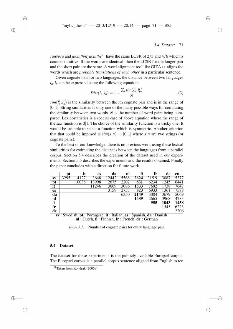
ii


ii

ii

5.4 Dataset 71

saw/osa and jacinth/hyacinthe21 have the same LCSR of 2/3 and 4/6 which iscounter-intuitive. If the words are identical, then the LCSR for the longer pairand the short pair are the same. A word alignment tool like GIZA++ aligns thewords which are probable translations of each other in a particular sentence.

Given cognate lists for two languages, the distance between two languagesla, lb can be expressed using the following equation:

Dist(la, lb) = 1− ∑i sim(lia, l

ib)

N(3)

sim(lia, l

ib) is the similarity between the ith cognate pair and is in the range of

[0,1]. String similarities is only one of the many possible ways for computingthe similarity between two words. N is the number of word pairs being com-pared. Lexicostatistics is a special case of above equation where the range ofthe sim function is 0|1. The choice of the similarity function is a tricky one. Itwould be suitable to select a function which is symmetric. Another criterionthat that could be imposed is sim(x,y)→ [0,1] where x,y are two strings (orcognate pairs).

To the best of our knowledge, there is no previous work using these lexicalsimilarities for estimating the distances between the languages from a parallelcorpus. Section 5.4 describes the creation of the dataset used in our experi-ments. Section 5.5 describes the experiments and the results obtained. Finallythe paper concludes with a direction for future work.

pt it es da nl fi fr de ensv 3295 4127 3648 12442 5568 2624 315 9 3087 5377pt 10038 13998 2675 2202 831 6234 1245 6441it 11246 3669 3086 1333 7692 1738 7647es 3159 2753 823 6933 1361 7588da 6350 2149 3004 3679 5069nl 1489 2665 3968 4783fi 955 1043 1458fr 1545 6223de 2206

sv : Swedish, pt : Portugese, it : Italian, es : Spanish, da : Danishnl : Dutch, fi : Finnish, fr : French, de : German

Table 5.1: Number of cognate pairs for every language pair.

5.4 Dataset

The dataset for these experiments is the publicly available Europarl corpus.The Europarl corpus is a parallel corpus sentence aligned from English to ten

21Taken from Kondrak (2005a)

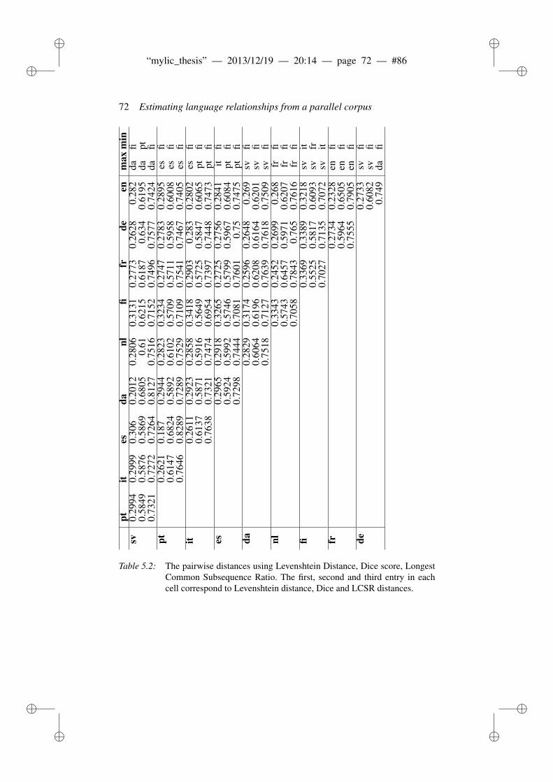
ii


ii

ii

72 Estimating language relationships from a parallel corpuspt

ites

danl

fifr

deen

max

min

sv0.

2994

0.29

990.

306

0.20

120.

2806

0.31

310.

2773

0.26

280.

282

dafi

0.58

490.

5876

0.58

690.

6805

0.61

0.62

150.

6187

0.63

40.

6195

dapt

0.73

210.

7272

0.72

640.

8127

0.75

160.

7152

0.74

960.

7577

0.74

24da

fipt

0.26

210.

187

0.29

440.

2823

0.32

340.

2747

0.27

830.

2895

esfi

0.61

470.

6824

0.58

920.

6102

0.57

090.

5711

0.59

580.

6008

esfi

0.76

460.

8289

0.72

890.

7529

0.71

090.

7541

0.74

670.

7405

esfi

it0.

2611

0.29

230.

2858

0.34

180.

2903

0.28

30.

2802

esfi

0.61

370.

5871

0.59

160.

5649

0.57

250.

5847

0.60

65pt

fi0.

7638

0.73

210.

7474

0.69

540.

7397

0.74

480.

7473

ptfi

es0.

2965

0.29

180.

3265

0.27

250.

2756

0.28

41it

fi0.

5924

0.59

920.

5746

0.57

990.

5967

0.60

84pt

fi0.

7298

0.74

440.

7081

0.76

010.

750.

7475

ptfi

da0.

2829

0.31

740.

2596

0.26

480.

269

svfi

0.60

640.

6196

0.62

080.

6164

0.62

01sv

fi0.

7518

0.71

270.

7639

0.76

180.

7509

svfi

nl0.

3343

0.24

520.

2699

0.26

8fr

fi0.

5743

0.64

570.

5971

0.62

07fr

fi0.

7058

0.78

430.

765

0.76

16fr

fifi

0.33

690.

3389

0.32

18sv

it0.

5525

0.58

170.

6093

svfr

0.70

270.

7135

0.70

72sv

itfr

0.27

340.

2328

enfi

0.59

640.

6505

enfi

0.75

550.

7905

enfi

de0.

2733

svfi

0.60

82sv

fi0.

749

dafi

Table 5.2: The pairwise distances using Levenshtein Distance, Dice score, LongestCommon Subsequence Ratio. The first, second and third entry in eachcell correspond to Levenshtein distance, Dice and LCSR distances.

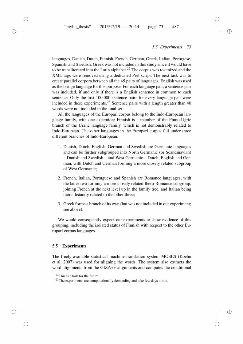
ii


ii

ii

5.5 Experiments 73

languages, Danish, Dutch, Finnish, French, German, Greek, Italian, Portugese,Spanish, and Swedish. Greek was not included in this study since it would haveto be transliterated into the Latin alphabet.22 The corpus was tokenized and theXML tags were removed using a dedicated Perl script. The next task was tocreate parallel corpora between all the 45 pairs of languages. English was usedas the bridge language for this purpose. For each language pair, a sentence pairwas included, if and only if there is a English sentence in common to eachsentence. Only the first 100,000 sentence pairs for every language pair wereincluded in these experiments.23 Sentence pairs with a length greater than 40words were not included in the final set.

All the languages of the Europarl corpus belong to the Indo-European lan-guage family, with one exception: Finnish is a member of the Finno-Ugricbranch of the Uralic language family, which is not demonstrably related toIndo-European. The other languages in the Europarl corpus fall under threedifferent branches of Indo-European:

1. Danish, Dutch, English, German and Swedish are Germanic languagesand can be further subgrouped into North Germanic (or Scandinavian)– Danish and Swedish – and West Germanic – Dutch, English and Ger-man, with Dutch and German forming a more closely related subgroupof West Germanic;

2. French, Italian, Portuguese and Spanish are Romance languages, withthe latter two forming a more closely related Ibero-Romance subgroup,joining French at the next level up in the family tree, and Italian beingmore distantly related to the other three;

3. Greek forms a branch of its own (but was not included in our experiment;see above).

We would consequently expect our experiments to show evidence of thisgrouping, including the isolated status of Finnish with respect to the other Eu-roparl corpus languages.

5.5 Experiments

The freely available statistical machine translation system MOSES (Koehnet al. 2007) was used for aligning the words. The system also extracts theword alignments from the GIZA++ alignments and computes the conditional

22This is a task for the future.23The experiments are computationally demanding and take few days to run.

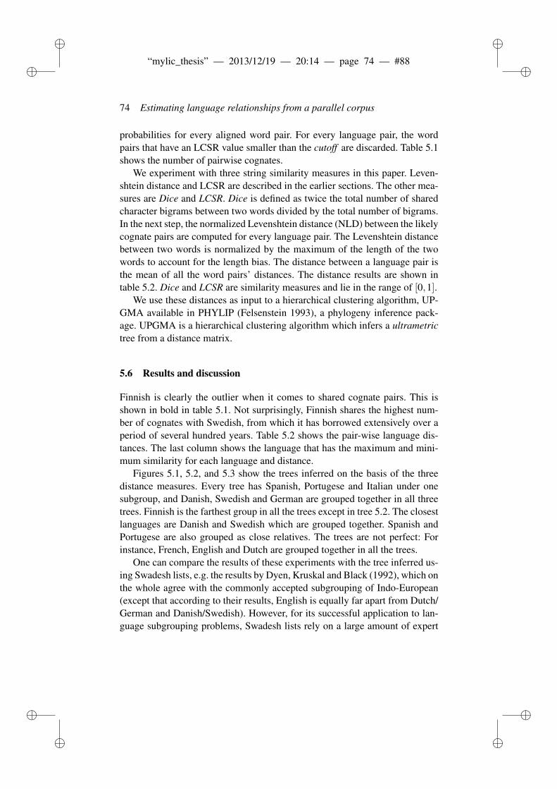
ii


ii

ii


probabilities for every aligned word pair. For every language pair, the wordpairs that have an LCSR value smaller than the cutoff are discarded. Table 5.1shows the number of pairwise cognates.

We experiment with three string similarity measures in this paper. Leven-shtein distance and LCSR are described in the earlier sections. The other mea-sures are Dice and LCSR. Dice is defined as twice the total number of sharedcharacter bigrams between two words divided by the total number of bigrams.In the next step, the normalized Levenshtein distance (NLD) between the likelycognate pairs are computed for every language pair. The Levenshtein distancebetween two words is normalized by the maximum of the length of the twowords to account for the length bias. The distance between a language pair isthe mean of all the word pairs’ distances. The distance results are shown intable 5.2. Dice and LCSR are similarity measures and lie in the range of [0,1].

We use these distances as input to a hierarchical clustering algorithm, UP-GMA available in PHYLIP (Felsenstein 1993), a phylogeny inference pack-age. UPGMA is a hierarchical clustering algorithm which infers a ultrametrictree from a distance matrix.

5.6 Results and discussion

Finnish is clearly the outlier when it comes to shared cognate pairs. This isshown in bold in table 5.1. Not surprisingly, Finnish shares the highest num-ber of cognates with Swedish, from which it has borrowed extensively over aperiod of several hundred years. Table 5.2 shows the pair-wise language dis-tances. The last column shows the language that has the maximum and mini-mum similarity for each language and distance.

Figures 5.1, 5.2, and 5.3 show the trees inferred on the basis of the threedistance measures. Every tree has Spanish, Portugese and Italian under onesubgroup, and Danish, Swedish and German are grouped together in all threetrees. Finnish is the farthest group in all the trees except in tree 5.2. The closestlanguages are Danish and Swedish which are grouped together. Spanish andPortugese are also grouped as close relatives. The trees are not perfect: Forinstance, French, English and Dutch are grouped together in all the trees.

One can compare the results of these experiments with the tree inferred us-ing Swadesh lists, e.g. the results by Dyen, Kruskal and Black (1992), which onthe whole agree with the commonly accepted subgrouping of Indo-European(except that according to their results, English is equally far apart from Dutch/German and Danish/Swedish). However, for its successful application to lan-guage subgrouping problems, Swadesh lists rely on a large amount of expert

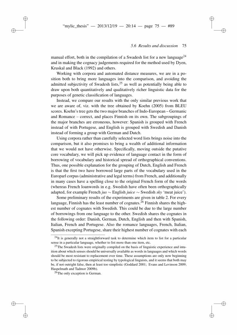
ii


ii

ii

5.6 Results and discussion 75

manual effort, both in the compilation of a Swadesh list for a new language24

and in making the cognacy judgements required for the method used by Dyen,Kruskal and Black (1992) and others.

Working with corpora and automated distance measures, we are in a po-sition both to bring more languages into the comparison, and avoiding theadmitted subjectivity of Swadesh lists,25 as well as potentially being able todraw upon both quantitatively and qualitatively richer linguistic data for thepurposes of genetic classification of languages.

Instead, we compare our results with the only similar previous work thatwe are aware of, viz. with the tree obtained by Koehn (2005) from BLEUscores. Koehn’s tree gets the two major branches of Indo-European – Germanicand Romance – correct, and places Finnish on its own. The subgroupings ofthe major branches are erroneous, however: Spanish is grouped with Frenchinstead of with Portugese, and English is grouped with Swedish and Danishinstead of forming a group with German and Dutch.

Using corpora rather than carefully selected word lists brings noise into thecomparison, but it also promises to bring a wealth of additional informationthat we would not have otherwise. Specifically, moving outside the putativecore vocabulary, we will pick up evidence of language contact in the form ofborrowing of vocabulary and historical spread of orthographical conventions.Thus, one possible explanation for the grouping of Dutch, English and Frenchis that the first two have borrowed large parts of the vocabulary used in theEuroparl corpus (administrative and legal terms) from French, and additionallyin many cases have a spelling close to the original French form of the words(whereas French loanwords in e.g. Swedish have often been orthographicallyadapted, for example French jus ∼ English juice ∼ Swedish sky ‘meat juice’).

Some preliminary results of the experiments are given in table 2. For everylanguage, Finnish has the least number of cognates.26 Finnish shares the high-est number of cognates with Swedish. This could be due to the large numberof borrowings from one language to the other. Swedish shares the cognates inthe following order: Danish, German, Dutch, English and then with Spanish,Italian, French and Portugese. Also the romance languages, French, Italian,Spanish excepting Portugese, share their highest number of cognates with each

24It is generally not a straightforward task to determine which item to list for a particularsense in a particular language, whether to list more than one item, etc.

25The Swadesh lists were originally compiled on the basis of linguistic experience and intu-ition about which senses should be universally available as words in languages and which wordsshould be most resistant to replacement over time. These assumptions are only now beginningto be subjected to rigorous empirical testing by typological linguists, and it seems that both maybe, if not outright false, then at least too simplistic (Goddard 2001; Evans and Levinson 2009;Haspelmath and Tadmor 2009b).

26The only exception is German.

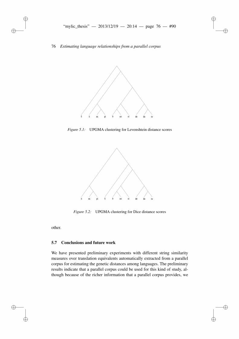
ii


ii

ii


Figure 5.1: UPGMA clustering for Levenshtein distance scores

Figure 5.2: UPGMA clustering for Dice distance scores

other.

5.7 Conclusions and future work

We have presented preliminary experiments with different string similaritymeasures over translation equivalents automatically extracted from a parallelcorpus for estimating the genetic distances among languages. The preliminaryresults indicate that a parallel corpus could be used for this kind of study, al-though because of the richer information that a parallel corpus provides, we

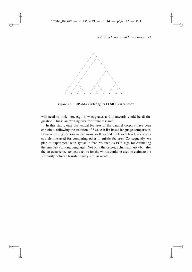
ii


ii

ii

5.7 Conclusions and future work 77

Figure 5.3: UPGMA clustering for LCSR distance scores

will need to look into, e.g., how cognates and loanwords could be distin-guished. This is an exciting area for future research.

In this study, only the lexical features of the parallel corpora have beenexploited, following the tradition of Swadesh list based language comparison.However, using corpora we can move well beyond the lexical level, as corporacan also be used for comparing other linguistic features. Consequently, weplan to experiment with syntactic features such as POS tags for estimatingthe similarity among languages. Not only the orthographic similarity but alsothe co-occurrence context vectors for the words could be used to estimate thesimilarity between translationally similar words.

ii


ii

ii

ii


ii

ii

6 N-GRAM APPROACHES TO

THE HISTORICAL DYNAMICS

OF BASIC VOCABULARY

Rama, Taraka and Lars Borin 2013. N-Gram Approaches to the Historical Dy-namics of Basic Vocabulary. Journal of Quantitative Linguistics 21 (1): 50–64.

Abstract

In this paper, we apply an information theoretic measure, self-entropy of phon-eme n-gram distributions, for quantifying the amount of phonological varia-tion in words for the same concepts across languages, thereby investigatingthe stability of concepts in a standardized concept list – based on the 100-itemSwadesh list – specifically designed for automated language classification. Ourfindings are consistent with those of the ASJP project (Automated SimilarityJudgment Program; Holman et al. 2008b). The correlation of our ranking withthat of ASJP is statistically highly significant. Our ranking also largely agreeswith two other reduced concept lists proposed in the literature. Our resultssuggest that n-gram analysis works at least as well as other measures for inves-tigating the relation of phonological similarity to geographical spread, auto-matic language classification, and typological similarity, while being compu-tationally considerably cheaper than the most widespread method (normalizedLevenshtein distance), very important when processing large quantities of lan-guage data.

6.1 Introduction

There are some 7,000 languages in the world (Lewis, Simons and Fennig2013). These can be grouped into 200–400 separate language families (Lewis,Simons and Fennig 2013; Dryer 2011; Hammarström 2010). Hammarström(2010: 198) defines a language family in this way (emphasis as in the original):

ii


ii

ii

80 N-gram approaches to the historical dynamics of basic vocabulary

– a set of languages (possibly a one-member set)– with at least one sufficiently attested member language– that has been demonstrated in publication– to stem from a common ancestor– by orthodox comparative methodology (Campbell and Poser 2008)– for which there are no convincing published attempts to demonstrate a

wider affiliation.This definition implies that the set of established language families may

change as research progresses, but also that there may be limits to what isknowable about the history of languages. Sometimes we find statements in theliterature to the effect that a hypothesized wider affiliation is too remote tobe recoverable using the traditional comparative method (Campbell and Poser2008: ch. 9–10).

However, only a very small minority of these language families are so well-studied that there is fair consensus among experts about their internal geneticsubgrouping – the structure of their family tree – at least in general outline. Forthe vast majority of the world’s languages, the work of confirming and sub-grouping established families and of combining them into more encompassingunits is still very much on the wish-list of historical-comparative linguistics.

This is a vast undertaking, and to boot one pursuing a receding goal, sincethe world’s languages are disappearing at an estimated rate of about one lan-guage every two weeks (Krauss 1992), many of them without leaving behindenough of a record so as to allow their genetic affiliations to be investigated inany detail. Here, as in other fields of scientific enquiry, we would do well to askourselves whether it would be possible to develop quantitative computationaltools that could help experts in this endeavor. One such tool is lexicostatistics,first explicitly articulated about a half-century ago by the American linguistMorris Swadesh in a series of oft-cited papers (Swadesh 1948, 1950, 1952,1955).

At the time – almost before computers – lexicostatistics was designed asa completely manual procedure. It relied on the manual calculation of degreeof overlap – the percentage of shared cognates27 – between short standardizedlists of central and universal senses, e.g., the so-called Swadesh lists contain-ing on the order of 200 (Swadesh 1952) or 100 items (Swadesh 1955). In lex-icostatistics as originally conceived, cognacy is always determined solely byhuman expert judgment.

The degree of overlap can be trivially calculated automatically once wehave the information about which items are cognates and thus are to be counted

27In the terminology of historical linguistics, items (words, morphemes or constructions)in related languages are cognates if they all descend directly from the same proto-languageitem. This is sometimes called vertical transmission, as opposed to horizontal transmission, i.e.,borrowing in a wide sense. Thus, cognacy in historical linguistics explicitly excludes loanwords.

ii


ii

ii

6.1 Introduction 81

as the same. Hence, the time-consuming bottleneck in lexicostatistics is thedetermination of cognacy, which requires considerable expertise and efforteven in the case of small language families (which is not where we wouldexpect to gain most from applying lexicostatistics in any case). Recently, someresearchers have for this reason turned to approaches more amenable to au-tomation, hoping that large-scale automatic language classification will thusbecome feasible.

It is important to stress at this point that such approaches are not intendedas an alternative to traditional historical-comparative linguistic methodology,but rather as an addition to its toolbox. If these methods live up to expectations,they will provide an initial screening and a good first approximation of possiblegenetic relationships among large numbers of languages, some of which canthen be singled out for more thorough investigation by human experts. Theresults of such investigations could then be brought back to inform and refinethe automated approaches.

In most of this work, explicit cognacy judgments are replaced by an auto-matic calculation crucially relying on some form of (string) similarity measure,based on the assumption that, on average, cognates will tend to be more similaracross languages than non-cognates. The outcome of the automated methodscan be tested by comparing the automatically calculated inter-language dis-tances to accepted language family subgroupings arrived at by the traditionalcomparative method, such as those provided in the Ethnologue (Lewis, Simonsand Fennig 2013) or the World Atlas of Language Structures (WALS; Haspel-math et al. 2011).

In this paper, our aim is to investigate an alternative similarity measure,phoneme n-gram distributions, in this context, comparing it to the currentlymost popular measure, a variant of Levenshtein distance.

The rest of the paper is structured as follows. In the next section we givesome necessary background information and a brief account of relevant re-lated work, including the design of the ASJP database, which we use in ourexperiments. In the following sections, we describe and motivate the methodwe propose for computing item stability across language families of the world,and report on the results obtained through the application of the method, com-paring them with earlier results reported in the literature. Finally, we discussthe implications of our rankings and indicate directions for further research.

ii


ii

ii


6.2 Background and related work

6.2.1 Item stability and Swadesh list design

In historical linguistics, item stability is defined as the degree of resistance ofan item to lexical replacement over time, either by another lexical item from thesame language or by a borrowed lexical item. The item itself may either go outof use and disappear from the language altogether, or acquire another meaning(semantic change), i.e., move into another item slot. For example, Old Englishdeor ‘animal’ > deer (compare the Swedish cognate djur ‘animal’, which hasnot undergone this shift in meaning). The modern English word animal is aborrowing from Old French.

The quest for a core vocabulary (list of central lexical items; see Borin2012 for a detailed discussion of some linguistic and computational linguisticaspects of core vocabularies) for language classification and dating of languagedivergence has been going on since the beginning of lexicostatistics (Swadesh1948, 1950, 1952, 1955). The initial list of 215 items, originally presentedby Swadesh in 1952, was reduced to a 100 item list in 1955. The items inthe Swadesh lists supposedly represent senses universally present in humanlanguages, and represented by words maximally resistant to lexical replace-ment. Unfortunately, the Swadesh lists were established mainly on the basis ofSwadesh’s own intuition and (considerable) professional linguistic experience,and were thus naturally limited in terms of the number of languages that couldbe taken into account.

Oswalt (1971) later attempted to provide more exact criteria for including aconcept in the Swadesh list: (1) The cognate set28 for the item should accountfor as many languages as possible. In other words, the number of cognate setsfor an item should be as small as possible. (2) Cognates found in far removedlanguages are a stronger indicator of stability than those found in closely re-lated languages.29

Together with the observation that cognates tend to be phonologically moresimilar than non-cognates – at least in the kind of vocabulary covered by theSwadesh lists – this opens the possibility to use (automatic) string similaritymeasures as proxies for (manual) cognacy judgments, thereby allowing us totest item stability on a large scale in order to investigate more objectively how

28The term cognate set refers to a set of cognate items, i.e., words in different languages goingback to the same proto-language word. In working with Swadesh lists, cognates are furtherrequired to express the same sense in order for them to be in the same cognate set.

29Compare English wheel to Hindi chakka ‘wheel’, which do not reveal themselves to becognates through visual inspection, but can nevertheless be traced back to the same Proto-Indo-European root.

ii


ii

ii

6.2 Background and related work 83

well-founded Swadesh’s intuitions were. To this end, Holman et al. (2008a) de-fined a measure – based on the phonological matches (measured using LDND;see below) between words for a single item in closely related languages (asdefined in terms of WALS genera of a family; see Dryer 2011) – to rank itemsin a 100-item Swadesh list as to their stability and to evaluate the effect ofthe word-list size on automatic language classification by comparing the auto-matically computed inter-language distances to the genetic classification givenin the WALS (Haspelmath et al. 2011) and Ethnologue (Lewis, Simons andFennig 2013). They found that the list could be pared down to a 40-item most-stable subset without impairing the classification significantly. The resultingstability ranking of the Swadesh list items will be used in our experiment de-scribed below.

At least two recent exhaustive evaluations in automatic language classifi-cation, by Pompei, Loreto and Tria (2011) and Wichmann et al. (2011a), vin-dicate the use of 40-item lists across the world’s language families. In bothcases, a tree building algorithm (Neighbour Joining; Saitou and Nei 1987) wasapplied to the LDND distance matrices and the resulting trees were comparedwith two expert classifications (Lewis 2009; Hammarström 2010) using threedifferent tree comparison measures, in all cases showing high agreement withthe expert classifications.

6.2.2 The ASJP database

The ASJP (Automated Similarity Judgment Program) project30 (Brown et al.2008), comprises a group of scholars who have embarked on an ambitious pro-gram of automating the computation of similarities between languages usinglexical similarity measures. The ASJP database covers a very large number oflanguages (more than half the world’s languages in the version of the databaseused in the present paper). For each language present in the database, it con-tains a short phonetically transcribed word list based on the 100-item Swadeshlist. For most of the languages this has been reduced down to the most stable40 items, according to the empirical findings of Holman et al. 2008a, describedabove.

These concepts are supposed to be highly stable dischronically and there-fore useful for estimating inter-language genetic distances. The ASJP programcomputes the distance between two languages as the average pair-wise length-normalized Levenshtein distance (Levenshtein 1966), called Levenshtein Dis-tance Normalized (LDN). LDN is further modified to compensate for chanceresemblance such as accidental phoneme inventory similarity between a pair

30http://email.eva.mpg.de/∼wichmann/ASJPHomePage.htm

ii


ii

ii


of languages to yield LDND (Levenshtein Distance Normalized Divided; Hol-man et al. 2008b).

The ASJP effort began with a small dataset of 100-item lists for 245 lan-guages. Since then, the ASJP database has been continually expanded, to in-clude in its latest version (v. 14) more than 5,500 word lists representing wellover one half of the languages of the world (Wichmann et al. 2011b). As men-tioned above, most of the added word lists have aimed to cover only the 40-item most stable Swadesh subset identified by Holman et al. (2008a), and notthe full 100-item list.

Each lexical item in an ASJP word list is transcribed in a broad phonetictranscription known as ASJP Code (Brown et al. 2008). The ASJP code con-sists of 34 consonant symbols, 7 vowels, and four modifiers, all rendered bycharacters available on the English version of the QWERTY keyboard. Tone,stress and vowel length are ignored in this format. The three modifiers combinesymbols to form phonologically complex segments (e.g., aspirated, glottalized,or nasalized segments).

6.2.3 Earlier n-gram-based approaches

In quantitative approaches to historical linguistics, there are at least two ear-lier lines of work where character n-grams have been used for computing thepair-wise distances between languages, in both cases based on multilingualcorpora rather than Swadesh-type word lists. Huffman (1998) compute pair-wise language distances based on character n-grams extracted from Bible textsin European and indigenous American languages (mostly from the Mayan lan-guage family). Singh and Surana (2007) use character n-grams extracted fromraw comparable corpora of ten languages from the Indian subcontinent forcomputing the pair-wise language distances between languages belonging totwo different language families (Indo-Aryan and Dravidian). Rama and Singh(2009) introduce a factored language model based on articulatory features toinduce a articulatory feature level n-gram model from the dataset of Singh andSurana 2007. The feature n-grams of each language pair are compared usingdistributional similarity measures such as cross-entropy to yield a single pointdistance between a language pair.

Being based on extensive naturalistic corpus data, these studies have theconsiderable positive aspect of empirical well-groundedness. On the negativeside, except for the study of Rama and Singh 2009, the real object of compar-ison – the phonology of the languages – is accessed only indirectly, throughtheir standard orthographies, which differ in various ways, potentially distort-ing the cross-linguistic comparison. Another shortcoming of using corpora for

ii


ii

ii

6.3 Method 85

large-scale cross-linguistic investigations stems from the fact that only a smallminority of the world’s languages have an established written form (Borin2009), and initiatives such as the “universal corpus of the world’s languages”of Abney and Bird 2010, although of course infinitely laudable, are still a verylong way from their realization.

6.3 Method

The work presented here considers a different approach from that of ASJP toinvestigate the individual relationship of phonological similarity with item sta-bility. The approach in this paper is inspired by the work of Cavnar and Trenkle1994, who use character n-grams for text categorization, based on their obser-vation that the n-grams for a particular document category follow a Zipfian dis-tribution. The rank of a character n-gram varies across documents belongingto different languages, topics and genres. Building upon this work, Dunning(1994) motivates the use of these character n-grams for automatic languageidentification and the computation of inter-language distances as well as dis-tances between dialects.

Our motivation for conducting the present investigation has been twofold:(1) There is a general lack of comparative studies in this area, and we thusaim to contribute to the general methodological development of the field; and(2) complexity-wise, an n-gram-based similarity calculation is much more ef-fective than LDND (linear vs. quadratic in the length of the input strings), andhence will scale up to much larger datasets, should the need for this arise (e.g.,for comparing corpus data or full-sized dictionaries, rather than the short wordlists used here).

For reasons given above, we depart from earlier n-gram-based approachesin that we do not use corpus data. Instead, we take advantage of the fact thatthe ASJP database offers an attractive alternative to corpora as the basis formassive cross-linguistic investigations. Wichmann, Rama and Holman (2011)show that the phoneme inventory sizes of 458 of the world’s languages (Mad-dieson and Precoda 1990) have a robust correlation (r = 0.61) with the numberof 1-grams (supposed phonemes) extracted from the word lists for the corre-sponding languages in the ASJP database. Given this result, it is reasonableto assume that the phoneme n-grams extracted from the ASJP database give afair picture of the phonology of the languages and consequently can be usedfor investigating item stability directly on the phonetic level.

All the experiments reported in this paper were performed on a subset ofversion 12 of the ASJP database.31 The database contains a total of 4,169 word

31Available on http://email.eva.mpg.de/~wichmann/listss12.zip.

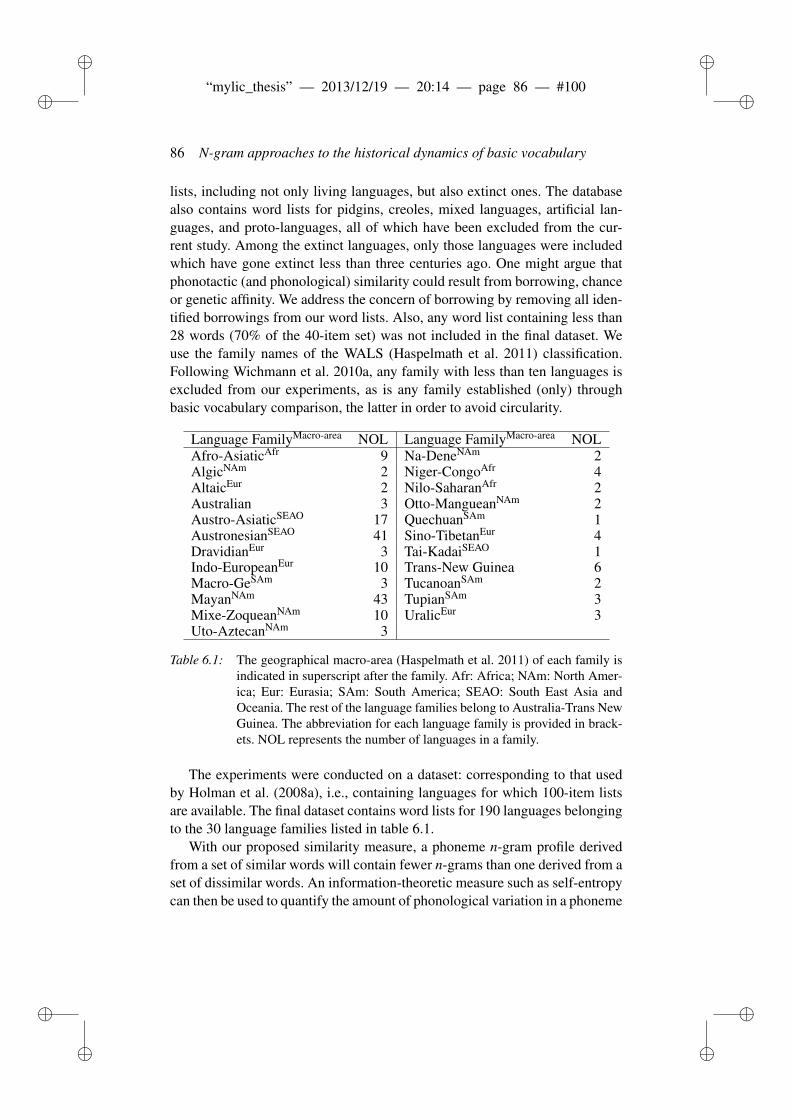
ii


ii

ii


lists, including not only living languages, but also extinct ones. The databasealso contains word lists for pidgins, creoles, mixed languages, artificial lan-guages, and proto-languages, all of which have been excluded from the cur-rent study. Among the extinct languages, only those languages were includedwhich have gone extinct less than three centuries ago. One might argue thatphonotactic (and phonological) similarity could result from borrowing, chanceor genetic affinity. We address the concern of borrowing by removing all iden-tified borrowings from our word lists. Also, any word list containing less than28 words (70% of the 40-item set) was not included in the final dataset. Weuse the family names of the WALS (Haspelmath et al. 2011) classification.Following Wichmann et al. 2010a, any family with less than ten languages isexcluded from our experiments, as is any family established (only) throughbasic vocabulary comparison, the latter in order to avoid circularity.

Language FamilyMacro-area NOL Language FamilyMacro-area NOLAfro-AsiaticAfr 9 Na-DeneNAm 2AlgicNAm 2 Niger-CongoAfr 4AltaicEur 2 Nilo-SaharanAfr 2Australian 3 Otto-MangueanNAm 2Austro-AsiaticSEAO 17 QuechuanSAm 1AustronesianSEAO 41 Sino-TibetanEur 4DravidianEur 3 Tai-KadaiSEAO 1Indo-EuropeanEur 10 Trans-New Guinea 6Macro-GeSAm 3 TucanoanSAm 2MayanNAm 43 TupianSAm 3Mixe-ZoqueanNAm 10 UralicEur 3Uto-AztecanNAm 3

Table 6.1: The geographical macro-area (Haspelmath et al. 2011) of each family isindicated in superscript after the family. Afr: Africa; NAm: North Amer-ica; Eur: Eurasia; SAm: South America; SEAO: South East Asia andOceania. The rest of the language families belong to Australia-Trans NewGuinea. The abbreviation for each language family is provided in brack-ets. NOL represents the number of languages in a family.

The experiments were conducted on a dataset: corresponding to that usedby Holman et al. (2008a), i.e., containing languages for which 100-item listsare available. The final dataset contains word lists for 190 languages belongingto the 30 language families listed in table 6.1.

With our proposed similarity measure, a phoneme n-gram profile derivedfrom a set of similar words will contain fewer n-grams than one derived from aset of dissimilar words. An information-theoretic measure such as self-entropycan then be used to quantify the amount of phonological variation in a phoneme

ii


ii

ii


n-gram profile, e.g., for a Swadesh-list item across a language family. Ourhypothesis is that this measure will work analogously to the LDND distancemeasure, and be a good, computationally cheaper substitute for it.

The phoneme n-gram profile for a language family is computed in the fol-lowing manner. A phoneme n-gram is defined as the consecutive phonemesegments in a window of a fixed length n. The value of n ranges from one tofive. All the phoneme 1-grams to 5-grams are extracted for a lexical item inan item list. All n-grams for an item, extracted from word-lists belonging to afamily, are merged, counted and sorted in order of descending frequency. Thislist constitutes the n-gram profile for the item. In the next step, the relativefrequency of each n-gram in an n-gram profile for an item is computed by nor-malizing the frequency of a phoneme n-gram by the sum of the frequencies ofall the n-grams in an item’s n-gram profile. This corresponds roughly to thelength normalization step in the calculation of LDND. It can be summarizedas in (4), where f i

ngram denotes the frequency of the ith n-gram and S denotesthe size of the n-gram profile for an item.

r f ingram =

f ingram

∑Si=1 f i

ngram(4)

Given this background, the self-entropy of the kth item’s n-gram profile candefined as in (5):

Hkitem =−

S

∑i=1

r f ingram · log(r f i

ngram) (5)

The self-entropy H(·) is further scaled by raising it to the power of e toprovide better resolution. Since self-entropy H(·) measures the amount of di-vergence in the phoneme n-gram profile for an item, the items can be rankedrelatively in terms of the ascending order of self-entropy averaged (weightedby the size of the family32) across the families.


Table 6.2 shows the 100 items ranked in decreasing order of stability, as indi-cated by the phoneme n-grams method. A Spearman’s rank correlation ρ be-tween the ranks given in table 6.2 and the ranks given by Holman et al. (2008a)

32We use weighted average to factor out the effect of sample size of each language family.We tried averaging using the number of families and total number of languages present in the100-word list sample. Both the averaging techniques correlate highly (ρ > 0.92, p < 0.001)with the weighted average.

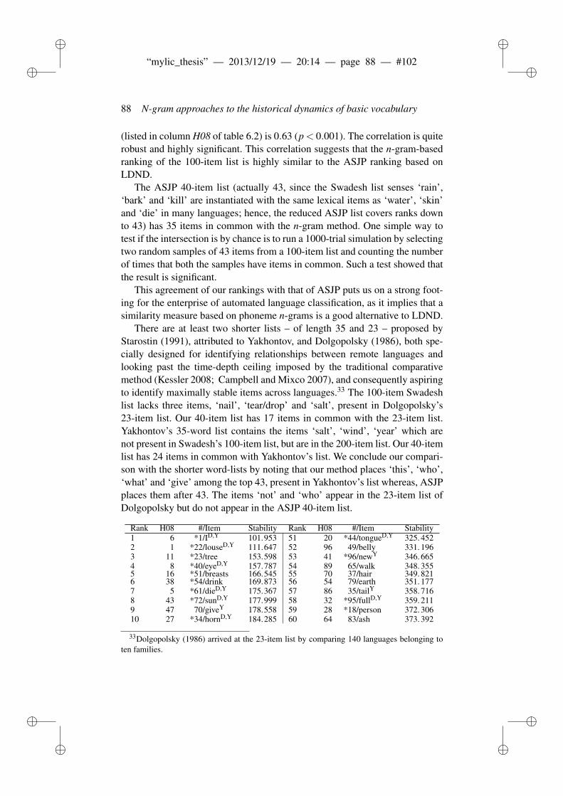
ii


ii

ii


(listed in column H08 of table 6.2) is 0.63 (p < 0.001). The correlation is quiterobust and highly significant. This correlation suggests that the n-gram-basedranking of the 100-item list is highly similar to the ASJP ranking based onLDND.

The ASJP 40-item list (actually 43, since the Swadesh list senses ‘rain’,‘bark’ and ‘kill’ are instantiated with the same lexical items as ‘water’, ‘skin’and ‘die’ in many languages; hence, the reduced ASJP list covers ranks downto 43) has 35 items in common with the n-gram method. One simple way totest if the intersection is by chance is to run a 1000-trial simulation by selectingtwo random samples of 43 items from a 100-item list and counting the numberof times that both the samples have items in common. Such a test showed thatthe result is significant.

This agreement of our rankings with that of ASJP puts us on a strong foot-ing for the enterprise of automated language classification, as it implies that asimilarity measure based on phoneme n-grams is a good alternative to LDND.

There are at least two shorter lists – of length 35 and 23 – proposed byStarostin (1991), attributed to Yakhontov, and Dolgopolsky (1986), both spe-cially designed for identifying relationships between remote languages andlooking past the time-depth ceiling imposed by the traditional comparativemethod (Kessler 2008; Campbell and Mixco 2007), and consequently aspiringto identify maximally stable items across languages.33 The 100-item Swadeshlist lacks three items, ‘nail’, ‘tear/drop’ and ‘salt’, present in Dolgopolsky’s23-item list. Our 40-item list has 17 items in common with the 23-item list.Yakhontov’s 35-word list contains the items ‘salt’, ‘wind’, ‘year’ which arenot present in Swadesh’s 100-item list, but are in the 200-item list. Our 40-itemlist has 24 items in common with Yakhontov’s list. We conclude our compari-son with the shorter word-lists by noting that our method places ‘this’, ‘who’,‘what’ and ‘give’ among the top 43, present in Yakhontov’s list whereas, ASJPplaces them after 43. The items ‘not’ and ‘who’ appear in the 23-item list ofDolgopolsky but do not appear in the ASJP 40-item list.

Rank H08 #/Item Stability Rank H08 #/Item Stability1 6 *1/ID,Y 101.953 51 20 *44/tongueD,Y 325. 4522 1 *22/louseD,Y 111.647 52 96 49/belly 331. 1963 11 *23/tree 153.598 53 41 *96/newY 346. 6654 8 *40/eyeD,Y 157.787 54 89 65/walk 348. 3555 16 *51/breasts 166.545 55 70 37/hair 349. 8216 38 *54/drink 169.873 56 54 79/earth 351. 1777 5 *61/dieD,Y 175.367 57 86 35/tailY 358. 7168 43 *72/sunD,Y 177.999 58 32 *95/fullD,Y 359. 2119 47 70/giveY 178.558 59 28 *18/person 372. 30610 27 *34/hornD,Y 184.285 60 64 83/ash 373. 392

33Dolgopolsky (1986) arrived at the 23-item list by comparing 140 languages belonging toten families.

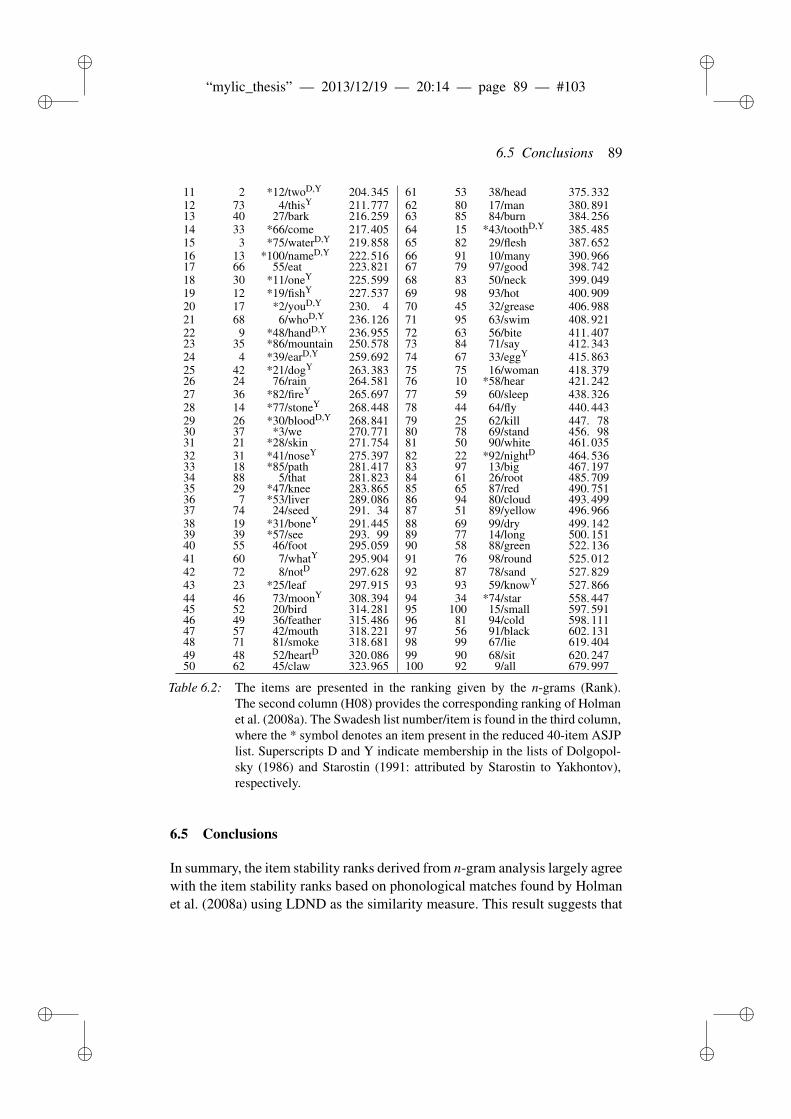
ii


ii

ii

6.5 Conclusions 89

11 2 *12/twoD,Y 204.345 61 53 38/head 375. 33212 73 4/thisY 211.777 62 80 17/man 380. 89113 40 27/bark 216.259 63 85 84/burn 384. 25614 33 *66/come 217.405 64 15 *43/toothD,Y 385. 48515 3 *75/waterD,Y 219.858 65 82 29/flesh 387. 65216 13 *100/nameD,Y 222.516 66 91 10/many 390. 96617 66 55/eat 223.821 67 79 97/good 398. 74218 30 *11/oneY 225.599 68 83 50/neck 399. 04919 12 *19/fishY 227.537 69 98 93/hot 400. 90920 17 *2/youD,Y 230. 4 70 45 32/grease 406. 98821 68 6/whoD,Y 236.126 71 95 63/swim 408. 92122 9 *48/handD,Y 236.955 72 63 56/bite 411. 40723 35 *86/mountain 250.578 73 84 71/say 412. 34324 4 *39/earD,Y 259.692 74 67 33/eggY 415. 86325 42 *21/dogY 263.383 75 75 16/woman 418. 37926 24 76/rain 264.581 76 10 *58/hear 421. 24227 36 *82/fireY 265.697 77 59 60/sleep 438. 32628 14 *77/stoneY 268.448 78 44 64/fly 440. 44329 26 *30/bloodD,Y 268.841 79 25 62/kill 447. 7830 37 *3/we 270.771 80 78 69/stand 456. 9831 21 *28/skin 271.754 81 50 90/white 461. 03532 31 *41/noseY 275.397 82 22 *92/nightD 464. 53633 18 *85/path 281.417 83 97 13/big 467. 19734 88 5/that 281.823 84 61 26/root 485. 70935 29 *47/knee 283.865 85 65 87/red 490. 75136 7 *53/liver 289.086 86 94 80/cloud 493. 49937 74 24/seed 291. 34 87 51 89/yellow 496. 96638 19 *31/boneY 291.445 88 69 99/dry 499. 14239 39 *57/see 293. 99 89 77 14/long 500. 15140 55 46/foot 295.059 90 58 88/green 522. 13641 60 7/whatY 295.904 91 76 98/round 525. 01242 72 8/notD 297.628 92 87 78/sand 527. 82943 23 *25/leaf 297.915 93 93 59/knowY 527. 86644 46 73/moonY 308.394 94 34 *74/star 558. 44745 52 20/bird 314.281 95 100 15/small 597. 59146 49 36/feather 315.486 96 81 94/cold 598. 11147 57 42/mouth 318.221 97 56 91/black 602. 13148 71 81/smoke 318.681 98 99 67/lie 619. 40449 48 52/heartD 320.086 99 90 68/sit 620. 24750 62 45/claw 323.965 100 92 9/all 679. 997

Table 6.2: The items are presented in the ranking given by the n-grams (Rank).The second column (H08) provides the corresponding ranking of Holmanet al. (2008a). The Swadesh list number/item is found in the third column,where the * symbol denotes an item present in the reduced 40-item ASJPlist. Superscripts D and Y indicate membership in the lists of Dolgopol-sky (1986) and Starostin (1991: attributed by Starostin to Yakhontov),respectively.

6.5 Conclusions

In summary, the item stability ranks derived from n-gram analysis largely agreewith the item stability ranks based on phonological matches found by Holmanet al. (2008a) using LDND as the similarity measure. This result suggests that

ii


ii

ii


phoneme n-grams work at least as well as other string similarity measures –e.g., LDND – for investigating the relation of phonological similarity to ge-ographical spread, automatic language classification, and typological similar-ity. At the same time, n-gram analysis is cheaper in terms of computationalresources – the fundamental comparison step has linear complexity, againstquadratic complexity for LDND – which is important when processing largequantities of language data.34

A topic in need of future research is a continuation of the methodologicalstrand of the work presented here, in the form of a more encompassing com-parison of different string similarity measures for automated lexicostatistics.There is also the general issue of whether the “classical” Swadesh lists are theoptimal point of departure for identifying the most stable lexical items acrossthe languages of the world, as has been (tacitly or explicitly) assumed in mostprevious work (with Dolgopolsky 1986 forming a notable exception in thisregard; see also Borin 2012 for a more in-depth discussion of this issue), orwhether even more stable items could be found by looking at the matter withfresh eyes, perhaps using text corpora.

34The LDND program takes about one hour to compute the inter-language distances whereas,the n-gram analysis takes less than two minutes.

ii


ii

ii

7 TYPOLOGICAL DISTANCES

AND LANGUAGE

CLASSIFICATION

Rama, Taraka and Prasanth Kolachina 2012. How good are typological dis-tances for determining genealogical relationships among languages? COLING(posters), 975–984.

Abstract

The recent availability of typological databases such as World Atlas of Lan-guage Structures (WALS) has spurred investigations regarding its utility forclassifying the world’s languages, the stability of typological features in ge-netic linguistics and typological universals across the language families of theworld. In this paper, we compare typological distances, derived from fifteenvector similarity measures, with family internal classifications and also lexi-cal divergence. These results are only a first step towards the use of WALSdatabase in the projection of NLP resources and bootstrapping NLP tools fortypologically or genetically similar, yet resource-poor languages.

7.1 Introduction

There are more than 7000 languages in this world (Lewis 2009), which fallinto more than 140 genetic families having descended from a common ances-tor. The aim of traditional historical linguistics is to trace the evolutionary path,a tree of extant languages to their extinct common ancestor. Genealogical rela-tionship is not the only characteristic which relates languages; languages canalso share structurally common features such as word order, similar phonemeinventory size and morphology. For instance, Finnish and Telugu, which aregeographically remote and yet have a agglutinative morphology. It would bea grave error to posit that two languages are genetically related due to a sin-gle common structural feature. There have been attempts in the past (Nichols1995) to rank the stability of structural features. Stability implies the resistance

ii


ii

ii

92 Typological distances and language classification

of a structural feature to change across space and time. For instance, Dravid-ian languages have adhered to subject-object-verb (SOV) word order for thelast two thousand years (Krishnamurti 2003; Dunn, Levinson and Lindström2008). Hence, it can be claimed that the structural feature SOV is very stablein Dravidian language family. Also, structural features have recently been usedfor inferring the evolutionary tree of a small group of Papuan languages of thePacific (Dunn et al. 2005).

In the area of computational linguistics, genealogical distances betweentwo language families have been shown to be useful for predicting the diffi-culty of machine translation (Birch, Osborne and Koehn 2008). However, theuse of typological distances in the development of various NLP tools largelyremains unexplored. Typologically similar languages provide useful leveragewhen working with low-resource languages. In this paper, we compare typo-logical distances with family internal classification and also within-family lex-ical divergence.

The paper is structured as followed. In section 7.2, we summarize the re-lated work. Section 7.3 lists the contributions of this work. Section 7.4 de-scribes the typological database, lexical database and the criteria for preparingthe final dataset. Section 7.5 presents the different vector similarity measuresand the evaluation procedure. The results of our experiments are given in Sec-tion 7.6. We conclude the paper and discuss the future directions in Section7.7.

7.2 Related Work

Dunn et al. (2005) were the first to apply a well-tested computational phy-logenetic method (from computational biology), Maximum Parsimony (MP;Felsenstein 2004) to typological features (phonological, syntactic and mor-phological). The authors used MP to classify a set of unrelated languages – inOceania – belonging to two different families. In another related work, Wich-mann and Saunders (2007) apply three different phylogenetic algorithms –Neighbor Joining (Saitou and Nei 1987), MP and Bayesian inference (Ron-quist and Huelsenbeck 2003) – to the typological features (from WALS) of 63native American languages. They also ranked the typological features in termsof stability. Nichols and Warnow (2008) survey the use of typological featuresfor language classification in computational historical linguistics. In a novelwork, Bakker et al. (2009) combine typological distances with lexical similar-ity to boost the language classification accuracy. As a first step, they computethe pair-wise typological distances for 355 languages, obtained through theapplication of length normalized Hamming distance to 85 typological features

ii


ii

ii

7.2 Related Work 93

(ranked by Wichmann and Holman 2009b). They combine the typological dis-tances with lexical divergence, derived from lexicostatistical lists, to boost lan-guage classification accuracy. Unfortunately, these works seem to have goneunnoticed in computational linguistics.

Typological feature such as phoneme inventory size (extracted from WALSdatabase; Haspelmath et al. 2011) was used by Atkinson (2011) to claim thatthe phoneme inventory size shows a negative correlation as one moves awayfrom Africa.35 In another work, Dunn et al. (2011) make an effort towardsdemonstrating that there are lineage specific trends in the word order universalsacross the families of the world.

In computational linguistics, Daume III (2009) and Georgi, Xia and Lewis(2010) use typological features from WALS for investigating relation betweenphylogenetic groups and feature stability. Georgi, Xia and Lewis (2010) moti-vate the use of typological features for projecting linguistic resources such astreebanks and bootstrapping NLP tools from “resource-rich” to “low-resource”languages which are genetically unrelated yet, share similar syntactic featuresdue to contact (ex., Swedish to Finnish or vice-versa). Georgi, Xia and Lewis(2010) compute pair-wise distances from typological feature vectors using co-sine similarity and a shared overlap measure (ratio of number of shared fea-tures to the total number of features, between a pair of feature vectors). Theyapply three different clustering algorithms – k-means, partitional, agglomera-tive – to the WALS dataset with number of clusters as testing parameter andobserve that the clustering performance measure (in terms of F-score) is not thebest when the number of clusters agree with the exact number of families (121)in the whole-world dataset. They find that the simplest clustering algorithm, k-means, wins across all the three datasets. However, the authors do not correctfor geographical bias in the dataset. Georgi, Xia and Lewis (2010) work withthree subsets of WALS database (after applying a pruning procedure describedin section 9.4). The first subset consists of 735 languages across the world.Both the second and third dataset are subsets of the first subset and consistof languages belonging to Indo-European and Sino-Tibetan language families.They divide their dataset into 10-folds and train the three clustering algorithmson 90% of the data to predict the remaining 10% of the features. Finally, thefeatures are ranked in the decreasing order of their prediction accuracy to yielda stability ranking of the features.

35Assuming a monogenesis hypothesis of language similar to the monogenesis hypothesis ofhomo sapiens.

ii


ii

ii


7.3 Contributions

In this article, we depart from Georgi, Xia and Lewis (2010) by not investigat-ing the much researched topics of feature stability and the feature predictionaccuracy of clustering measures. Rather, we try to answer the following ques-tions:• Do we really need a clustering algorithm to measure the internal classifi-

cation accuracy of a language family? Internal classification accuracy isa measure of closeness of the typological distances to the internal struc-ture of a language family.• How well do the typological distances within a family correlate with

the lexical distances derived from lexicostatistical lists (Swadesh 1952;Wichmann et al. 2011b), originally proposed for language classification?• Given that there are more than dozen vector similarity measures, which

vector similarity measure is the best for the above mentioned tasks?

7.4 Database

In this section, we describe WALS and Automated Similarity Judgment Pro-gram (ASJP), the two databases used in our experiments.

7.4.1 WALS

The WALS database36 has 144 feature types for 2676 languages distributedacross the globe. As noted by Hammarström (2009), the WALS database issparse across many language families of the world and the dataset needs prun-ing before it is used for further investigations. The database is represented asmatrix of languages vs. features. The pruning of the dataset has to be done inboth the directions to avoid sparsity when computing the pair-wise distancesbetween languages. Following Georgi, Xia and Lewis 2010, we remove all thelanguages which have less than 25 attested features. We also remove featureswith less than 10% attestations. This leaves the dataset with 1159 languagesand 193 features. Our dataset includes only those families having more than10 languages (following Wichmann et al. 2010a), shown in table 7.1. Georgi,Xia and Lewis (2010) work with a pruned dataset of 735 languages and twomajor families Indo-European and Sino-Tibetan whereas, we stick to inves-tigating the questions in section 7.3 for the well-defined language families –Austronesian, Afro-Asiatic – given in table 7.1.

36Accessed on 2011-09-22.

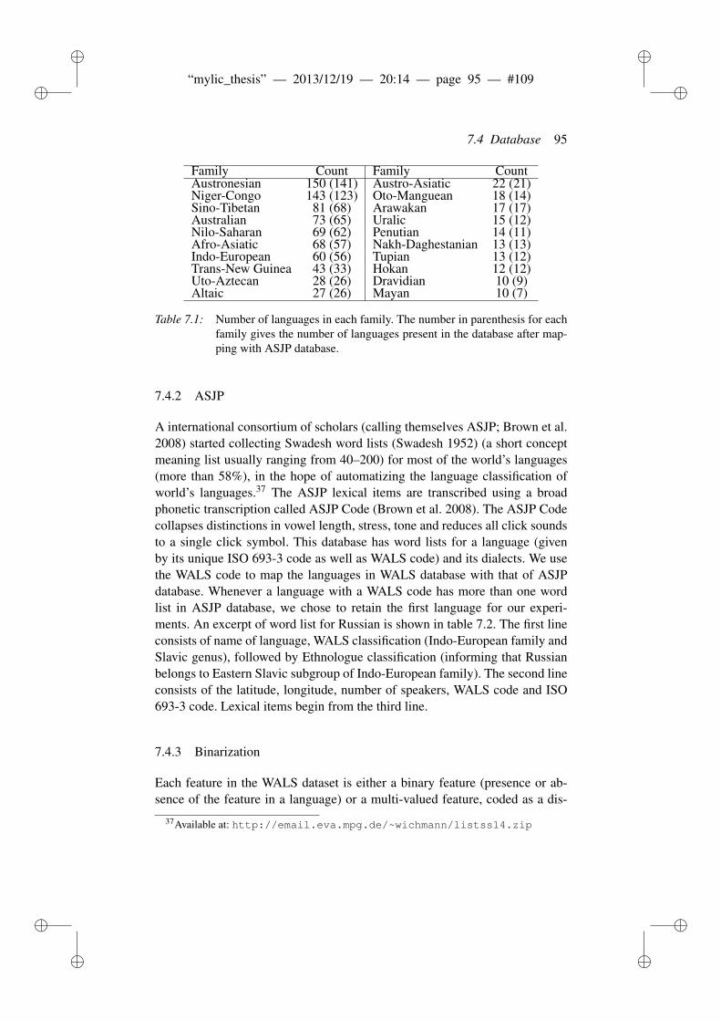
ii


ii

ii

7.4 Database 95

Family Count Family CountAustronesian 150 (141) Austro-Asiatic 22 (21)Niger-Congo 143 (123) Oto-Manguean 18 (14)Sino-Tibetan 81 (68) Arawakan 17 (17)Australian 73 (65) Uralic 15 (12)Nilo-Saharan 69 (62) Penutian 14 (11)Afro-Asiatic 68 (57) Nakh-Daghestanian 13 (13)Indo-European 60 (56) Tupian 13 (12)Trans-New Guinea 43 (33) Hokan 12 (12)Uto-Aztecan 28 (26) Dravidian 10 (9)Altaic 27 (26) Mayan 10 (7)

Table 7.1: Number of languages in each family. The number in parenthesis for eachfamily gives the number of languages present in the database after map-ping with ASJP database.

7.4.2 ASJP

A international consortium of scholars (calling themselves ASJP; Brown et al.2008) started collecting Swadesh word lists (Swadesh 1952) (a short conceptmeaning list usually ranging from 40–200) for most of the world’s languages(more than 58%), in the hope of automatizing the language classification ofworld’s languages.37 The ASJP lexical items are transcribed using a broadphonetic transcription called ASJP Code (Brown et al. 2008). The ASJP Codecollapses distinctions in vowel length, stress, tone and reduces all click soundsto a single click symbol. This database has word lists for a language (givenby its unique ISO 693-3 code as well as WALS code) and its dialects. We usethe WALS code to map the languages in WALS database with that of ASJPdatabase. Whenever a language with a WALS code has more than one wordlist in ASJP database, we chose to retain the first language for our experi-ments. An excerpt of word list for Russian is shown in table 7.2. The first lineconsists of name of language, WALS classification (Indo-European family andSlavic genus), followed by Ethnologue classification (informing that Russianbelongs to Eastern Slavic subgroup of Indo-European family). The second lineconsists of the latitude, longitude, number of speakers, WALS code and ISO693-3 code. Lexical items begin from the third line.

7.4.3 Binarization

Each feature in the WALS dataset is either a binary feature (presence or ab-sence of the feature in a language) or a multi-valued feature, coded as a dis-

37Available at: http://email.eva.mpg.de/~wichmann/listss14.zip

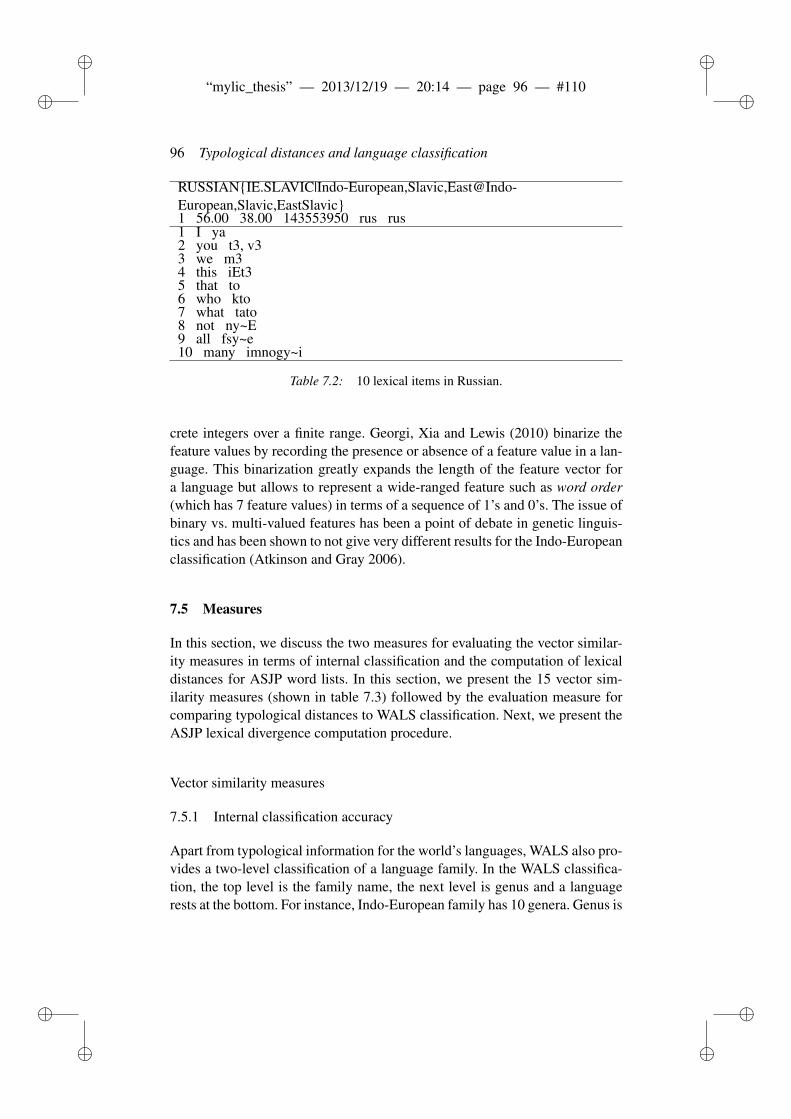
ii


ii

ii


RUSSIAN{IE.SLAVIC|Indo-European,Slavic,East@Indo-European,Slavic,EastSlavic}1 56.00 38.00 143553950 rus rus1 I ya2 you t3, v33 we m34 this iEt35 that to6 who kto7 what tato8 not ny~E9 all fsy~e10 many imnogy~i

Table 7.2: 10 lexical items in Russian.

crete integers over a finite range. Georgi, Xia and Lewis (2010) binarize thefeature values by recording the presence or absence of a feature value in a lan-guage. This binarization greatly expands the length of the feature vector fora language but allows to represent a wide-ranged feature such as word order(which has 7 feature values) in terms of a sequence of 1’s and 0’s. The issue ofbinary vs. multi-valued features has been a point of debate in genetic linguis-tics and has been shown to not give very different results for the Indo-Europeanclassification (Atkinson and Gray 2006).

7.5 Measures

In this section, we discuss the two measures for evaluating the vector similar-ity measures in terms of internal classification and the computation of lexicaldistances for ASJP word lists. In this section, we present the 15 vector sim-ilarity measures (shown in table 7.3) followed by the evaluation measure forcomparing typological distances to WALS classification. Next, we present theASJP lexical divergence computation procedure.

Vector similarity measures

7.5.1 Internal classification accuracy

Apart from typological information for the world’s languages, WALS also pro-vides a two-level classification of a language family. In the WALS classifica-tion, the top level is the family name, the next level is genus and a languagerests at the bottom. For instance, Indo-European family has 10 genera. Genus is

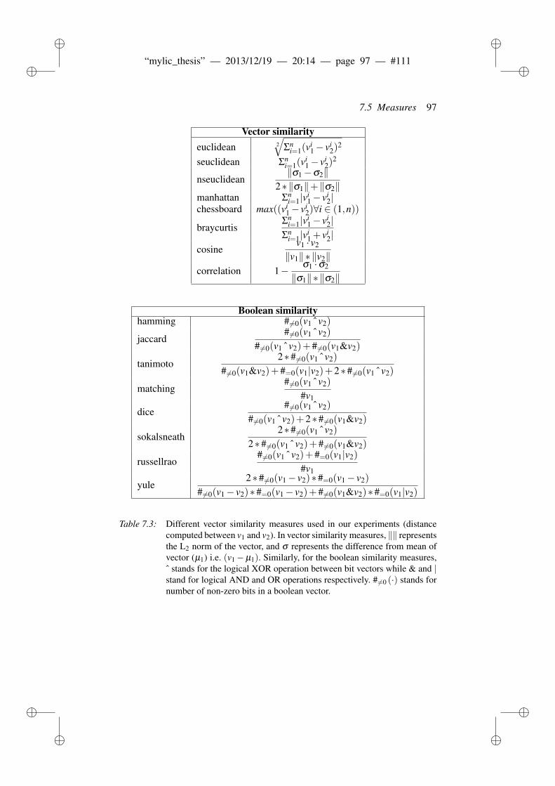
ii


ii

ii

7.5 Measures 97

Vector similarityeuclidean 2

√Σn

i=1(vi1− vi

2)2

seuclidean Σni=1(v

i1− vi

2)2

nseuclidean‖σ1−σ2‖

2∗‖σ1‖+‖σ2‖manhattan Σn

i=1|vi1− vi

2|chessboard max((vi

1− vi2)∀i ∈ (1,n))

braycurtisΣn

i=1|vi1− vi

2|Σn

i=1|vi1 + vi

2|cosine

v1 · v2

‖v1‖∗‖v2‖correlation 1− σ1 ·σ2

‖σ1‖∗‖σ2‖

Boolean similarityhamming #6=0(v1 ˆ v2)

jaccard#6=0(v1 ˆ v2)

# 6=0(v1 ˆ v2)+#6=0(v1&v2)

tanimoto2∗# 6=0(v1 ˆ v2)

#6=0(v1&v2)+#=0(v1|v2)+2∗# 6=0(v1 ˆ v2)

matching#6=0(v1 ˆ v2)

#v1

dice#6=0(v1 ˆ v2)

#6=0(v1 ˆ v2)+2∗# 6=0(v1&v2)

sokalsneath2∗# 6=0(v1 ˆ v2)

2∗#6=0(v1 ˆ v2)+# 6=0(v1&v2)

russellrao#6=0(v1 ˆ v2)+#=0(v1|v2)

#v1

yule2∗# 6=0(v1− v2)∗#=0(v1− v2)

# 6=0(v1− v2)∗#=0(v1− v2)+#6=0(v1&v2)∗#=0(v1|v2)

Table 7.3: Different vector similarity measures used in our experiments (distancecomputed between v1 and v2). In vector similarity measures, ‖‖ representsthe L2 norm of the vector, and σ represents the difference from mean ofvector (µ1) i.e. (v1−µ1). Similarly, for the boolean similarity measures,ˆ stands for the logical XOR operation between bit vectors while & and |stand for logical AND and OR operations respectively. #6=0 (·) stands fornumber of non-zero bits in a boolean vector.

ii


ii

ii


a consensually defined unit and not a rigorously established genealogical unit(Hammarström 2009). Rather, a genus corresponds to a group of languageswhich are supposed to have descended from a proto-language which is about3500 to 4000 years old. For instance, WALS lists Indic and Iranian languagesas separate genera whereas, both the genera are actually descendants of Proto-Indo-Iranian which in turn descended from Proto-Indo-European – a fact well-known in historical linguistics (Campbell and Poser 2008).

The WALS classification for each language family listed in table 7.1, canbe represented as a 2D-matrix with languages along both rows and columns.Each cell of such a matrix represents the WALS relationship in a language pairin the family. A cell has 0 if a language pair belong to the same genus and 1 ifthey belong to different genera. The pair-wise distance matrix obtained fromeach vector similarity measure is compared to the 2D-matrix using a specialcase of pearson’s r, called point-biserial correlation (Tate 1954).

7.5.2 Lexical distance

The ASJP program computes the distance between two languages as the aver-age pair-wise length-normalized Levenshtein distance, called Levenshtein Dis-tance Normalized (LDN) (Levenshtein 1966). LDN is further modified to ac-count for chance resemblance such as accidental phoneme inventory similaritybetween a pair of languages to yield LDND (Levenshtein Distance NormalizedDivided; Holman et al. 2008b). The performance of LDND distance matriceswas evaluated against two expert classifications of world’s languages in at leasttwo recent works (Pompei, Loreto and Tria 2011; Wichmann et al. 2011a).Their findings confirm that the LDND matrices largely agree with the classi-fication given by historical linguists. This result puts us on a strong ground touse ASJP’s LDND as a measure of lexical divergence within a family.

The distribution of the languages included in this study is plotted in figure7.1.

The correlation between typological distances and lexical distances is (with-in a family) computed as the Spearman’s rank correlation ρ between the typo-logical and lexical distances for all language pairs in the family. It is worthnoting that Bakker et al. (2009) also compare LDND distance matrices withWALS distance matrices for 355 languages from various families using a pear-son’s r whereas, we compare within-family LDND matrices with WALS dis-tance matrices derived from 15 similarity measures.

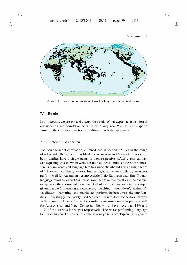
ii


ii

ii

7.6 Results 99

Figure 7.1: Visual representation of world’s languages in the final dataset.

7.6 Results

In this section, we present and discuss the results of our experiments in internalclassification and correlation with lexical divergence. We use heat maps tovisualize the correlation matrices resulting from both experiments.

7.6.1 Internal classification

The point bi-serial correlation, r, introduced in section 7.5, lies in the rangeof −1 to +1. The value of r is blank for Arawakan and Mayan families sinceboth families have a single genus in their respective WALS classifications.Subsequently, r is shown in white for both of these families. Chessboard mea-sure is blank across all language families since chessboard gives a single scoreof 1 between two binary vectors. Interestingly, all vector similarity measuresperform well for Australian, Austro-Asiatic, Indo-European and, Sino-Tibetanlanguage families, except for ‘russellrao’. We take this result as quite encour-aging, since they consist of more than 33% of the total languages in the samplegiven in table 7.1. Among the measures, ‘matching’, ‘seuclidean’, ‘tanimoto’,‘euclidean’, ‘hamming’ and ‘manhattan’ perform the best across the four fam-ilies. Interestingly, the widely used ‘cosine’ measure does not perform as wellas ‘hamming’. None of the vector similarity measures seem to perform wellfor Austronesian and Niger-Congo families which have more than 14% and11% of the world’s languages respectively. The worst performing languagefamily is Tupian. This does not come as a surprise, since Tupian has 5 genera

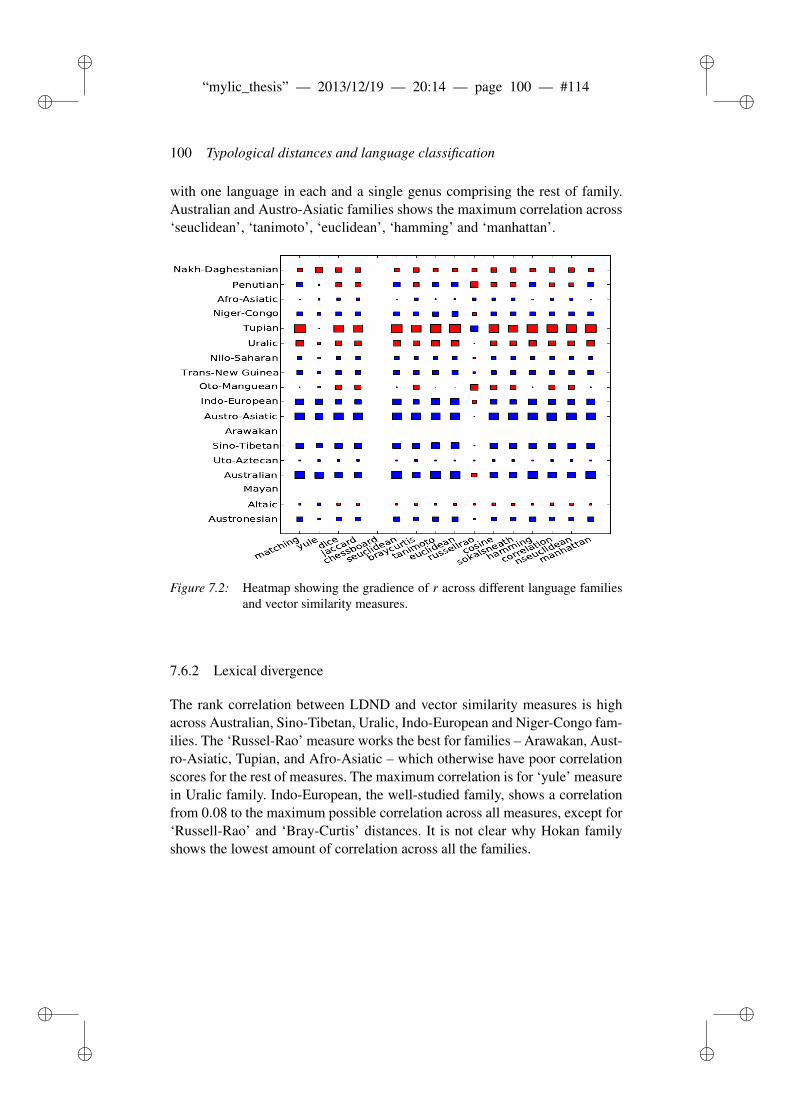
ii


ii

ii


with one language in each and a single genus comprising the rest of family.Australian and Austro-Asiatic families shows the maximum correlation across‘seuclidean’, ‘tanimoto’, ‘euclidean’, ‘hamming’ and ‘manhattan’.

Figure 7.2: Heatmap showing the gradience of r across different language familiesand vector similarity measures.

7.6.2 Lexical divergence

The rank correlation between LDND and vector similarity measures is highacross Australian, Sino-Tibetan, Uralic, Indo-European and Niger-Congo fam-ilies. The ‘Russel-Rao’ measure works the best for families – Arawakan, Aust-ro-Asiatic, Tupian, and Afro-Asiatic – which otherwise have poor correlationscores for the rest of measures. The maximum correlation is for ‘yule’ measurein Uralic family. Indo-European, the well-studied family, shows a correlationfrom 0.08 to the maximum possible correlation across all measures, except for‘Russell-Rao’ and ‘Bray-Curtis’ distances. It is not clear why Hokan familyshows the lowest amount of correlation across all the families.

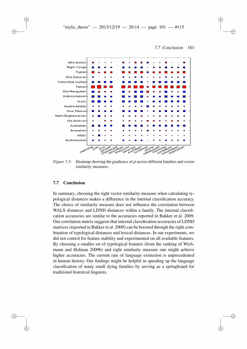
ii


ii

ii

7.7 Conclusion 101

Figure 7.3: Heatmap showing the gradience of ρ across different families and vectorsimilarity measures.

7.7 Conclusion

In summary, choosing the right vector similarity measure when calculating ty-pological distances makes a difference in the internal classification accuracy.The choice of similarity measure does not influence the correlation betweenWALS distances and LDND distances within a family. The internal classifi-cation accuracies are similar to the accuracies reported in Bakker et al. 2009.Our correlation matrix suggests that internal classification accuracies of LDNDmatrices (reported in Bakker et al. 2009) can be boosted through the right com-bination of typological distances and lexical distances. In our experiments, wedid not control for feature stability and experimented on all available features.By choosing a smaller set of typological features (from the ranking of Wich-mann and Holman 2009b) and right similarity measure one might achievehigher accuracies. The current rate of language extinction is unprecedentedin human history. Our findings might be helpful in speeding up the languageclassification of many small dying families by serving as a springboard fortraditional historical linguists.

ii


ii

ii

ii


ii

ii

8 PHONOTACTIC DIVERSITY

AND TIME DEPTH OF

LANGUAGE FAMILIES

Rama, Taraka 2013. Phonotactic Diversity Predicts the Time Depth of theWorld’s Language Families. PloS one 8.5:e63238.

Abstract

The ASJP (Automated Similarity Judgment Program) described an automated,lexical similarity-based method for dating the world’s language groups us-ing 52 archaeological, epigraphic and historical calibration date points. Thepresent paper describes a new automated dating method, based on phonotacticdiversity. Unlike ASJP, our method does not require any information on theinternal classification of a language group. Also, the method can use all theavailable word lists for a language and its dialects eschewing the debate of‘language’ and ‘dialect’. We further combine these dates and provide a newbaseline which, to our knowledge, is the best one. We make a systematic com-parison of our method, ASJP’s dating procedure, and combined dates. We pre-dict time depths for world’s language families and sub-families using this newbaseline. Finally, we explain our results in the model of language change givenby Nettle.

8.1 Introduction

Glottochronology, as introduced by Swadesh (1952, 1955), is a method forestimating the split/divergence time of two phylogenetically related languagesfrom their common ancestor. It makes use of Swadesh lists, which are shortlists, usually 100—215 items of core vocabulary, supposed to be resistant toborrowing and is universal and culture-free.

Core vocabulary is supposedly more resistant to lexical replacement thanother vocabulary items. There is an assumption of a universal constant rateof lexical change over time. The time depth of the point of split between two

ii


ii

ii

104 Phonotactic diversity and time depth of language families

languages is proportional to the logarithm of lexical similarity. The lexicalsimilarity between two languages is measured as the percentage of cognates,C, shared between the pair of languages. The time depth is estimated in unitsof 1000 years using the following formula.

t =log C

2 log r(6)

The constant r is experimentally determined by Lees (1953) using 13 controlcases.

Glottochronology was heavily criticized for several reasons, especially thefollowing ones:

• The composition of the core vocabulary list is not objective. Only re-cently, in Holman et al. 2008a; Petroni and Serva 2011 was the as-sumption of stability of the core vocabulary tested quantitatively for theworldwide language families.

• The rate of lexical replacement is not constant across different familiesor within the families. As demonstrated in Bergsland and Vogt 1962,Icelandic has a relatively lower rate of lexical change and East Green-landic Eskimo has a higher rate of lexical change than assumed by Lees(1953).

The related work in the field of computational historical linguistics is de-scribed in the next subsection.

8.1.1 Related work

The last decade has seen a surge in the number of papers published in historicallinguistics applying computational and statistical methods. This literature canbe broadly classified into two areas.

One area of work, represented by Wichmann et al. (2010a), Holman et al.(2008a), Bakker et al. (2009), Holman et al. (2011), Ringe, Warnow and Taylor(2002), and Gray and Atkinson (2003) focuses on collecting word lists forvarious language families for attacking classical historical linguistics problemssuch as dating, internal language classification, and lexical stability.

The other area of work, represented by papers such as Wichmann andHolman (2009a), Wichmann (2010b), Nettle (1999a), Wichmann, Müller andVelupillai (2010), Hammarström (2010), and Atkinson (2011) is characterizedby the application of quantitative methods to seek answers to questions alsoinvolving socio-historical processes, including the relations between language

ii


ii

ii

8.1 Introduction 105

diversity, human population sizes, agricultural patterns and geographical ori-gins of languages. It should be noted that this classification is not strictly mu-tually exclusive (see Wichmann 2008 for a survey of the computational, sta-tistical and inter-disciplinary work on language dynamics and change). Of theseveral works cited above, those of Wichmann et al. 2010a, Serva and Petroni2008, Holman et al. 2011 are relevant to this paper.

Gray and Atkinson (2003) date the Indo-European family as 8000 yearsold using a penalized minimum likelihood model which supports the Ana-tolian hypothesis of language spread. They use a binarily encoded charactermatrix (presence/absence of a cognate for a language; judged by comparativemethod) for Indo-European from Dyen, Kruskal and Black 1992 for inferringthe phylogenetic tree and dating its nodes.

A completely different approach is taken by the ASJP consortium for theautomated dating of the world’s language families. ASJP38 is a group of schol-ars who have embarked on an ambitious program of achieving an automatedclassification of world’s languages based on lexical similarity. As a means to-wards this end the group has embarked upon collecting Swadesh lists for allof the world’s languages. The database is described in the subsection ASJPDatabase below.

Holman et al. (2011) collected calibration points for 52 language groupsfrom archaeological, historical and epigraphic sources. The intra-language gro-up lexical similarity was computed using a version of the Levenshtein distance(LD). Levenshtein distance is defined as the minimum number of substitution,deletion and insertion operations required to convert a word to another word.This number is normalized by the maximum of the length of the two wordsto yield LDN, and finally the distance measure used, LDND (LDN Doublenormalized), is obtained by dividing the average LDN for all the word pairsinvolving the same meaning by the average LDN for all the word pairs involv-ing different meanings. The second normalization is done to compensate forchance lexical similarity due to similar phoneme inventories between unrelatedlanguages.

Now, we describe the computation of average lexical similarity for a intra-language group using the Scandinavian calibration point. The Scandinavianlanguage group has two sub-groups: East Scandinavian with 5 word lists andWest Scandinavian with 2 word lists. The internal classification information isobtained from Ethnologue (Lewis 2009). The ASJP procedure sums the LDNDof the 10 language pairs and divides them by 10 to yield an average LDND forScandinavian language group. Then, they fit a ordinary least-squares regres-sion model with average lexical similarity as a predictor and time depth as the

38http://email.eva.mpg.de/$~$wichmann/ASJPHomePage.htm

ii


ii

ii


response variable. The regression yields a highly robust correlation of −.84.Finally, they use the fitted regression model to predict a language group’s an-cestral time depth for different language families across the world.

Serva and Petroni (2008) were the first to use LD to estimate the time-depthof a language family. But their experiments were focused on dating the root ofthe Indo-European tree. They primarily use IE database (Dyen, Kruskal andBlack 1992) – augmented by some of their own data – for their experiments.

8.2 Materials and Methods

8.2.1 ASJP Database

The ASJP database (Wichmann et al. 2010b; Expanded versions of the ASJPdatabase are continuously being made available at 39) has 4817 word lists fromaround half of the languages of the world including creoles, dialects, artificiallanguages and extinct languages. We work with the version 13 database forcomparability with the results given by the ASJP dating procedure. A lan-guage and its dialects is identified through a unique ISO 639-3 code given inEthnologue (Lewis, Simons and Fennig 2013). The database also contains thelanguages’ genetic classification as given in WALS (Haspelmath et al. 2011)and Ethnologue (Lewis, Simons and Fennig 2013). The database has a shorterversion – the 40 most stable meanings empirically determined by Holman et al.(2008a) – of the original Swadesh list. A word list for a language is normallynot entered into the database if it has less than 70% of the 40 items. For our ex-periments, we use a subset of the data obtained by removing all the languagesextinct before 1700 CE.

The word lists in ASJP database are transcribed in ASJPcode (Brown et al.2008). ASJPcode consists of characters found on a QWERTY keyboard. ASJP-code has 34 consonant symbols and 7 vowel symbols. The different symbolscombine to form complex phonological segments. Vowel nasalization and glot-talization are indicated by ∗ and ” , respectively. Modifiers ∼ and $ indicatethat the preceding two or three segments are to be treated as a single symbol.

8.2.2 ASJP calibration procedure

The motivation for and the details of the ASJP calibration procedure is outlinedin this section. There are at least three processes by which the lexical similar-ity between genetically related languages decreases over time. Shared inher-

39http://email.eva.mpg.de/$~$wichmann/EarlierWorldTree.htm

ii


ii

ii

8.2 Materials and Methods 107

ited words (cognates) undergo regular sound changes to yield phonologicallyless similar words over time (e.g. English/Armenian two ∼ erku ‘two’; En-glish/Hindi wheel ∼ chakra ‘wheel’). Words can also undergo semantic shiftor are replaced through copying from other languages causing a decrement inthe lexical similarity between related languages. LDND is designed specifi-cally to capture the net lexical similarity between languages related throughdescent.

The ASJP’s date calibration formula is similar to that of glottochronology(6). Eqn. 6 implies that the ancestral language is lexically homogeneous att = 0. This formula is modified to accommodate lexical heterogeneity of theancestral language at time zero by introducing s0, representing average lexicalsimilarity at t = 0 of the language groups’ ancestral language. The cognateproportion C is replaced by the ASJP lexical similarity defined as 1−LDND.The formula then looks as in (2):

t = (log s− log s0)/2 log r (7)

The values of s0 and r are empirically determined by fitting a linear regressionmodel between the 52 language groups’ time depth (t) and their lexical similar-ity (s). The intra-language group similarity is defined as the average pairwiselexical similarity between the languages belonging to the coordinate subgroupsat the highest level of classification. Eqn. 7 and the negative correlation impliesthat log lexical similarity has an inverse linear relationship with time depth.

The next subsection describes our findings on the relation between languagegroup diversity and the age of the group.

8.2.3 Language group size and dates

As mentioned earlier, the ASJP consortium (Holman et al. 2011) collectedcommon ancestor divergence dates for 52 language groups, based on archae-ological, historical or epigraphic evidence. Written records can be used to de-termine the date of divergence of the common ancestral language reliably. Therecorded history of the speakers of the languages can be used to determine thedivergence dates based on major historical events. Since written records do notexist for temporally deep language families, the date for the common ancestormust often be inferred from archaeological sources.

Archaeological dates can be determined on the basis of traceability of theproto-language’s reconstructed words to excavated material objects. Dates canalso be inferred if loanwords can be correlated with historical or archaeologi-cal events. The process of compiling calibration points was extremely careful

ii


ii

ii


and archaeological calibration points were only included if they were non-controversial. Specifically, any glottochronologically determined date was ex-cluded from the sample.

A description of the sources of the dating points, the language groups’ sub-grouping adopted for computing the ASJP similarity, and also the ASJP simi-larity is available in the original paper. We wrote a python program to automat-ically extract the languages for a given group based on the description given inthe original paper. The data for number of languages, calibration date, type ofthe date, the genetic family, the mode of subsistence (pastoral or agriculture;from the compilation of Hammarström 2010), and the geographic area (basedon the continents Eurasia, Africa, Oceania, the Americas) for each languagegroup are given in table A.1.

First, we tested whether the sheer size of the language group (LGS) is re-lated to the calibration dates. The size was determined by counting the numberof languages in each language group, using Ethnologue (Lewis, Simons andFennig 2013). A scatter plot with time depth against LGS (on a log-log scale)shows a linear relationship. The regression, shown in figure 8.1, is r = .81and highly significant (p < 0.001). The linear relationship is shown by a solidstraight regression line. The younger dates are closer to the regression line thanthe older archaeological dates. figure 8.1 also displays the box plots of eachvariable along its axis. The box plot of LGS shows three outliers for groupslarger than 400, which are farther away from the rest of the dates but not fromthe regression line. The dotted line is the locally fitted polynomial regressionline (LOESS; with degree 2). The LOESS line stays close to the linear regres-sion line confirming that using a linear regression analysis is appropriate. Thesquare root of the variance of the residuals for the LOESS line is also shownas dotted lines on both the sides of the LOESS line.

Although this approach does not require the subgrouping information it isnot without problems. The ASJP database often has word lists from dialectsof a single language. The ASJP calibration procedure described in ASJP cal-ibration procedure subsection includes all the dialect word lists for a singlelanguage identified by its ISO code. Similarly, the LGS variable also countsthe total number of available word lists for a language group as its size.40

Nettle (1999a) summarizes the ‘language’ vs. ‘dialect’ judgmental difficultieswhen adopting language counts from Ethnologue for quantifying language di-versity (number of languages spoken per unit area). In another work, Nordhoffand Hammarström (2011) use the term ‘doculect’ to indicate a linguistic vari-ety identified in its descriptive resource. They use this definition to list various

40We obtain a Pearson’s r = .81 when LGS variable is counted as the number of languagesgiven in Ethnologue (Lewis, Simons and Fennig 2013).

ii


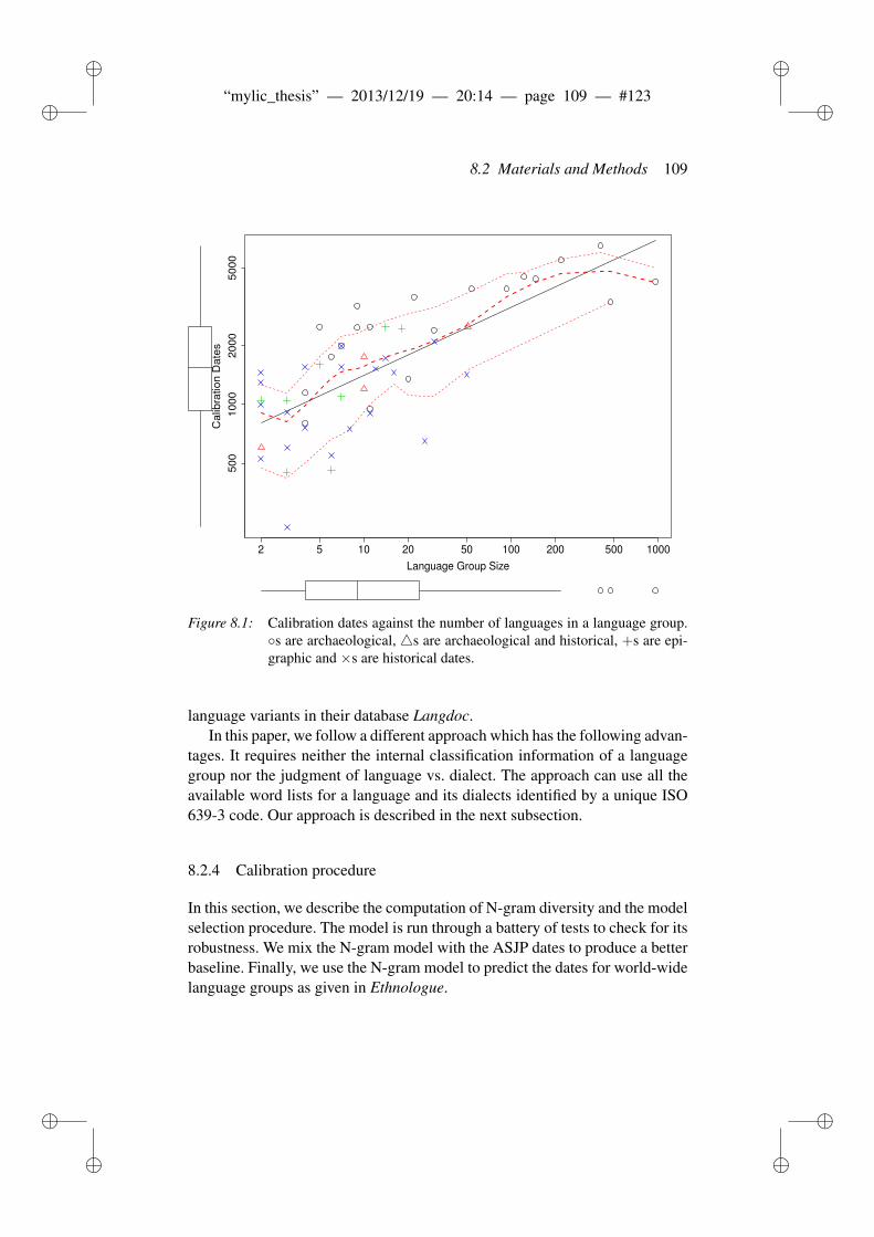
ii

ii

8.2 Materials and Methods 109

2 5 10 20 50 100 200 500 1000

500

1000

2000

5000

Language Group Size

Calib

ration D

ate

s

Figure 8.1: Calibration dates against the number of languages in a language group.◦s are archaeological, 4s are archaeological and historical, +s are epi-graphic and ×s are historical dates.

language variants in their database Langdoc.In this paper, we follow a different approach which has the following advan-

tages. It requires neither the internal classification information of a languagegroup nor the judgment of language vs. dialect. The approach can use all theavailable word lists for a language and its dialects identified by a unique ISO639-3 code. Our approach is described in the next subsection.

8.2.4 Calibration procedure

In this section, we describe the computation of N-gram diversity and the modelselection procedure. The model is run through a battery of tests to check for itsrobustness. We mix the N-gram model with the ASJP dates to produce a betterbaseline. Finally, we use the N-gram model to predict the dates for world-widelanguage groups as given in Ethnologue.

ii


ii

ii


8.2.5 N-grams and phonotactic diversity

N-grams are ubiquitous in natural language processing (NLP) and computa-tional linguistics, where they are used in systems ranging from statistical ma-chine translation to speech recognition, but they are relatively unknown in his-torical linguistics. N-grams are defined as a subsequence of length N from asequence of items. The items could be part-of-speech tags, words, morphemes,characters or phonemes. N-grams were originally introduced as a probabilis-tic model for predicting the next linguistic item, given a history of linguisticitems (Jurafsky and Martin 2000). The word “oxen” has four letter 1-grams‘o’,‘x’,‘e’,‘n’; three letter 2-grams ‘ox’, ‘xe’, ‘en’; two letter 3-grams ‘oxe’,‘xen’ and one letter 4-gram ‘oxen’. In general, any sequence of length n hasn−N +1 N-grams. The number of N-grams can similarly be calculated for aword in an ASJP word list for a given language.

Having introduced N-grams, we now define the phonological diversity ofa language and show how it can be computed using N-grams. Phonologicaldiversity for a language is defined as the size of its phoneme inventory. In asimilar fashion, the phonotactic diversity is defined as the total number of pos-sible phoneme combinations in a language. For a language, the 1-gram diver-sity (computed from a sufficiently long random list of phonetically transcribedwords) is the same as phonological diversity. Extending it further, the phono-tactic diversity can be computed as the N-gram diversity (N > 1). Given thatthe ASJP database (with its wide coverage) is a database of relatively short, 40-item word lists, it needs to be investigated whether the total number of uniquephonological segments represented in the 40 item word list can be used as aproxy for the actual phoneme inventory of a language.

Wichmann, Rama and Holman (2011) report a strong positive linear cor-relation of r = .61 between the phoneme inventory sizes for a sample of 392of the world’s languages, from the UPSID database (Maddieson and Precoda1990) and the number of phonological segments (which is the same as the 1-gram diversity) represented in word lists for the corresponding languages inthe ASJP database. The mean ratio of the ASJP segment size to the UPSIDinventory size is .817 and the standard deviation is .188. Also, there is a smallcorrelation (Pearson’s r = .17) between the size of the word list, which canvary from 28 to 40, and the number of ASJP phonological segments. This putsus on a solid ground before proceeding to use N-grams, extracted from theword lists, for purposes of calibrating dates.

The wide coverage of the ASJP database allows us to provide reasonablerelative estimates of the total number of phonological sequences (using ASJP-code) present in the world’s languages. Since ASJP modifiers∼ and $ combinethe preceding two or three symbols and there are 41 ASJP symbols in total, the

ii


ii

ii

8.3 Results and Discussion 111

number of theoretically possible phonological sequences is: 41+412 +413 =70,643. But the total number of ASJP sequences varies from 500 to 600 acrossall languages in the database depending on the criterion for extracting lan-guages from the ASJP database.

The N-gram (N ∈ [1,5]) diversity of a language group is defined as the setof all the combined unique phonological segments of length N for the lan-guages in the group. One might assume that N-grams are not a signature of alanguage group or, in other words, that N-grams do not distinguish unrelatedlanguage families from each other. However, it can be empirically establishedthat N-grams are more successful in distinguishing unrelated languages fromeach other than LDND. Wichmann et al. (2010a) devised a measure calleddist41 for measuring the efficacy of a lexical similarity measure (in this caseLDND vs. LDN) in distinguishing related languages vs. unrelated languages.In a separate experiment, which we will only briefly summarize here, usingASJP data from 49 of the worlds’ language families, we employed a 2-grambased measure, Dice,42 for quantifying the distance between the language fam-ilies and observed that it outperforms LDND in terms of dist. This empiricalresult shows that the set of N-grams of a language family is a genetic markerfor identifying related vs. unrelated languages.

8.3 Results and Discussion

Objective judgment of shared inheritance of words in related languages be-comes increasingly difficult due to the phonological distinctions accumulatedover time. We hypothesize that N-gram diversity for a language group is a non-decreasing function of time. To verify our hypothesis we check the nature ofrelationship between N-grams and dates. The last row in figure 8.2 shows thescatterplots of calibration dates (CD; given in table A.1) vs. N-grams. The lastcolumn of the upper triangular matrix displays significant correlations and thehighest correlation between 2-grams and CD. Both 3-grams and 1-grams showa similar correlation with CD whereas, 4-grams and 5-grams show a lower buta similar correlation. Another non-parametric test, Kendall’s τ , between theN-gram diversity and CD produces a relatively lower but highly significantcorrelation (p < 0.001). The highly significant ρ for different N-grams showsthat the hypothesis holds for different orders of N-grams.

Further, there is a highly significant ρ between N-gram diversity and group

41Dist of a family is defined as the difference between intra-family distance and inter-familydistances divided by the standard deviation of the inter-family distances.

42Between two strings: defined as twice the number of shared bigrams (2-grams) divided bythe total number of bigrams.

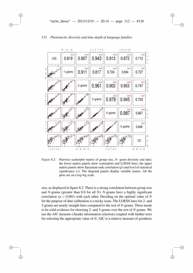
ii


ii

ii


LGS

3.0 4.0 5.0

0.819***

0.907***

4 5 6 7 8 9

0.943***

0.913***

3 4 5 6 7 8 9

0.872***

13

57

0.712***

3.0

4.0

5.0

1−grams 0.911***

0.817***

0.724***

0.654***

0.727***

2−grams 0.961***

0.902***

0.853***

4.5

5.5

6.5

7.5

0.747***

45

67

89

3−grams 0.978***

0.945***

0.723***

4−grams 0.987***

46

8

0.667***

35

79

5−grams 0.646***

1 2 3 4 5 6 7 4.5 5.5 6.5 7.5 4 5 6 7 8 9 5.5 6.5 7.5 8.5

5.5

7.0

8.5

CD

Figure 8.2: Pairwise scatterplot matrix of group size, N−gram diversity and date;the lower matrix panels show scatterplots and LOESS lines; the uppermatrix panels show Spearman rank correlation (ρ) and level of statisticalsignificance (?). The diagonal panels display variable names. All theplots are on a log-log scale.

size, as displayed in figure 8.2. There is a strong correlation between group sizeand N-grams (greater than 0.8 for all N). N-grams have a highly significantcorrelation (p < 0.001) with each other. Deciding on the optimal value of Nfor the purpose of date calibration is a tricky issue. The LOESS lines for 2- and3-grams are nearly straight lines compared to the rest of N-grams. There needsto be solid evidence for choosing 2- and 3-grams over the rest of N-grams. Weuse the AIC measure (Akaike information criterion) coupled with further testsfor selecting the appropriate value of N. AIC is a relative measure of goodness

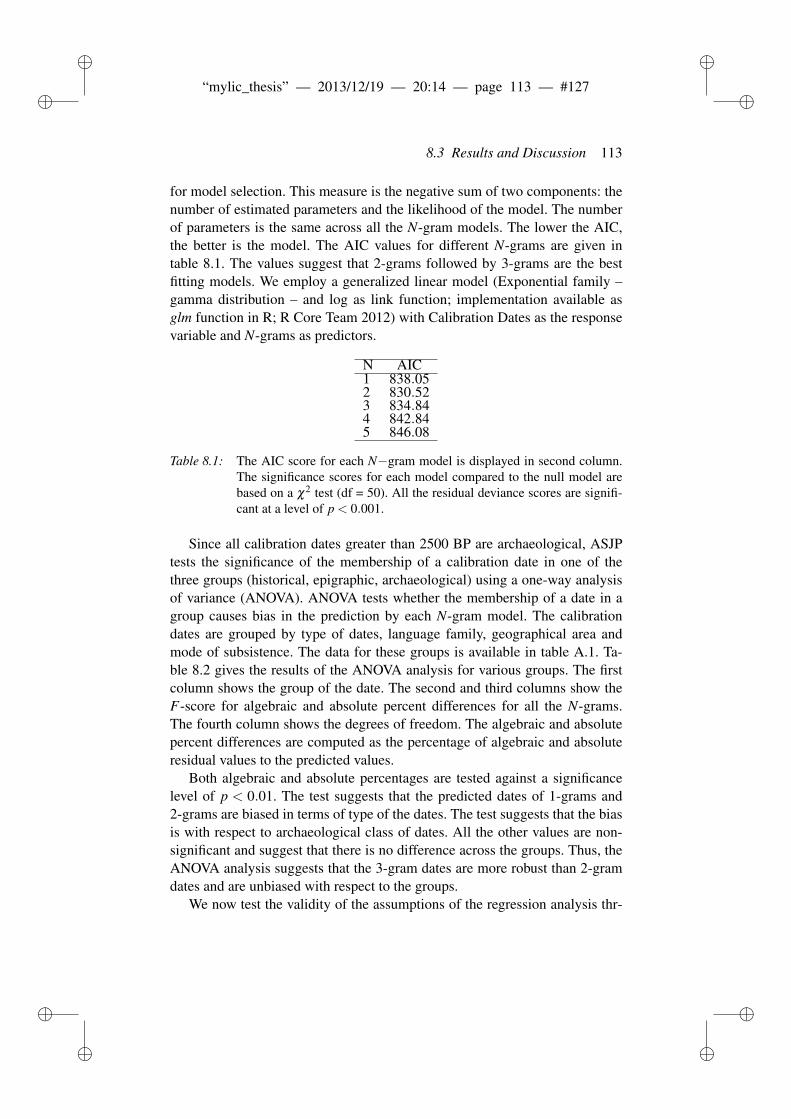
ii


ii

ii


for model selection. This measure is the negative sum of two components: thenumber of estimated parameters and the likelihood of the model. The numberof parameters is the same across all the N-gram models. The lower the AIC,the better is the model. The AIC values for different N-grams are given intable 8.1. The values suggest that 2-grams followed by 3-grams are the bestfitting models. We employ a generalized linear model (Exponential family –gamma distribution – and log as link function; implementation available asglm function in R; R Core Team 2012) with Calibration Dates as the responsevariable and N-grams as predictors.

N AIC1 838.052 830.523 834.844 842.845 846.08

Table 8.1: The AIC score for each N−gram model is displayed in second column.The significance scores for each model compared to the null model arebased on a χ2 test (df = 50). All the residual deviance scores are signifi-cant at a level of p < 0.001.

Since all calibration dates greater than 2500 BP are archaeological, ASJPtests the significance of the membership of a calibration date in one of thethree groups (historical, epigraphic, archaeological) using a one-way analysisof variance (ANOVA). ANOVA tests whether the membership of a date in agroup causes bias in the prediction by each N-gram model. The calibrationdates are grouped by type of dates, language family, geographical area andmode of subsistence. The data for these groups is available in table A.1. Ta-ble 8.2 gives the results of the ANOVA analysis for various groups. The firstcolumn shows the group of the date. The second and third columns show theF-score for algebraic and absolute percent differences for all the N-grams.The fourth column shows the degrees of freedom. The algebraic and absolutepercent differences are computed as the percentage of algebraic and absoluteresidual values to the predicted values.

Both algebraic and absolute percentages are tested against a significancelevel of p < 0.01. The test suggests that the predicted dates of 1-grams and2-grams are biased in terms of type of the dates. The test suggests that the biasis with respect to archaeological class of dates. All the other values are non-significant and suggest that there is no difference across the groups. Thus, theANOVA analysis suggests that the 3-gram dates are more robust than 2-gramdates and are unbiased with respect to the groups.

We now test the validity of the assumptions of the regression analysis thr-

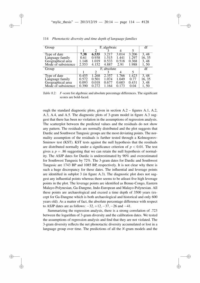
ii


ii

ii


Group F, algebraic df1 2 3 4 5

Type of date 7.38 6.535 3.217 3.014 3.206 3, 48Language family 0.61 0.938 1.515 1.441 1.297 16, 35Geographical area 1.148 1.019 0.533 0.518 0.368 3, 48Mode of subsistence 2.553 4.152 4.887 2.91 1.988 1, 50Group F, absolute df

1 2 3 4 5Type of date 0.455 1.268 2.357 1.766 1.423 3, 48Language family 0.572 0.501 1.074 1.049 0.77 16, 35Geographical area 0.093 0.018 0.677 0.603 0.431 3, 48Mode of subsistence 0.390 0.272 1.164 0.173 0.04 1, 50

Table 8.2: F-score for algebraic and absolute percentage differences. The significantscores are bold-faced.

ough the standard diagnostic plots, given in section A.2 – figures A.1, A.2,A.3, A.4, and A.5. The diagnostic plots of 3-gram model in figure A.3 sug-gest that there has been no violation in the assumptions of regression analysis.The scatterplot between the predicted values and the residuals do not showany pattern. The residuals are normally distributed and the plot suggests thatDardic and Southwest Tungusic groups are the most deviating points. The nor-mality assumption of the residuals is further tested through a Kolmogorov-Smirnov test (KST). KST tests against the null hypothesis that the residualsare distributed normally under a significance criterion of p < 0.01. The testgives a p = .86 suggesting that we can retain the null hypothesis of normal-ity. The ASJP dates for Dardic is underestimated by 90% and overestimatedfor Southwest Tungusic by 72%. The 3-gram dates for Dardic and SouthwestTungusic are 1743 BP and 1085 BP, respectively. It is not clear why there issuch a huge discrepancy for these dates. The influential and leverage pointsare identified in subplot 3 (in figure A.3). The diagnostic plot does not sug-gest any influential points whereas there seems to be atleast five high leveragepoints in the plot. The leverage points are identified as Benue-Congo, EasternMalayo-Polynesian, Ga-Dangme, Indo-European and Malayo-Polynesian. Allthese points are archaeological and exceed a time depth of 3500 years (ex-cept for Ga-Dangme which is both archaeological and historical and only 600years old). As a matter of fact, the absolute percentage difference with respectto ASJP dates are as follows: −32,+12,−37,−26 and −41.

Summarizing the regression analysis, there is a strong correlation of .723between the logarithm of 3-gram diversity and the calibration dates. We testedthe assumptions of regression analysis and find that they are not violated. The3-gram diversity reflects the net phonotactic diversity accumulated or lost in alanguage group over time. The predictions of all the N-gram models and the

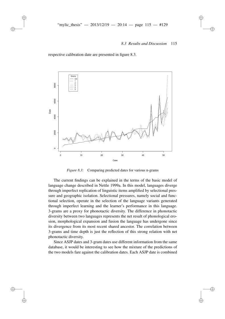
ii


ii

ii


respective calibration date are presented in figure 8.3.

0 10 20 30 40 50

02

00

04

00

06

00

08

00

0

Case

Da

te

Grams

CD

1

2

3

4

5

Figure 8.3: Comparing predicted dates for various n-grams

The current findings can be explained in the terms of the basic model oflanguage change described in Nettle 1999a. In this model, languages divergethrough imperfect replication of linguistic items amplified by selectional pres-sure and geographic isolation. Selectional pressures, namely social and func-tional selection, operate in the selection of the language variants generatedthrough imperfect learning and the learner’s performance in this language.3-grams are a proxy for phonotactic diversity. The difference in phonotacticdiversity between two languages represents the net result of phonological ero-sion, morphological expansion and fusion the language has undergone sinceits divergence from its most recent shared ancestor. The correlation between3-grams and time depth is just the reflection of this strong relation with netphonotactic diversity.

Since ASJP dates and 3-gram dates use different information from the samedatabase, it would be interesting to see how the mixture of the predictions ofthe two models fare against the calibration dates. Each ASJP date is combined

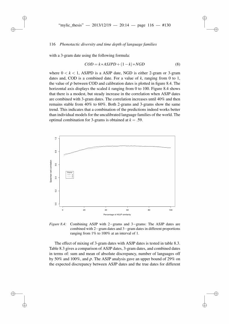
ii


ii

ii


with a 3-gram date using the following formula:

COD = k ∗ASJPD+(1− k)∗NGD (8)

where 0 < k < 1, ASJPD is a ASJP date, NGD is either 2-gram or 3-gramdates and, COD is a combined date. For a value of k, ranging from 0 to 1,the value of ρ between COD and calibration dates is plotted in figure 8.4. Thehorizontal axis displays the scaled k ranging from 0 to 100. Figure 8.4 showsthat there is a modest, but steady increase in the correlation when ASJP datesare combined with 3-gram dates. The correlation increases until 40% and thenremains stable from 40% to 60%. Both 2-grams and 3-grams show the sametrend. This indicates that a combination of the predictions indeed works betterthan individual models for the uncalibrated language families of the world. Theoptimal combination for 3-grams is obtained at k = .59.

0 20 40 60 80 100

0.0

0.2

0.4

0.6

0.8

1.0

Percentage of ASJP similarity

Sp

ea

rma

n r

an

k co

rre

latio

n

Grams

32

Figure 8.4: Combining ASJP with 2−grams and 3−grams: The ASJP dates arecombined with 2−gram dates and 3−gram dates in different proportionsranging from 1% to 100% at an interval of 1.

The effect of mixing of 3-gram dates with ASJP dates is tested in table 8.3.Table 8.3 gives a comparison of ASJP dates, 3-gram dates, and combined datesin terms of: sum and mean of absolute discrepancy, number of languages offby 50% and 100%, and ρ . The ASJP analysis gave an upper bound of 29% onthe expected discrepancy between ASJP dates and the true dates for different

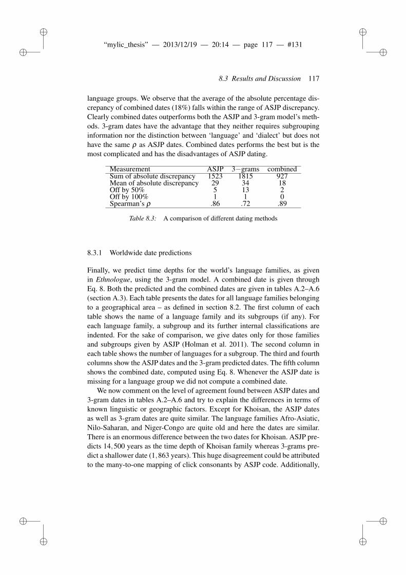
ii


ii

ii


language groups. We observe that the average of the absolute percentage dis-crepancy of combined dates (18%) falls within the range of ASJP discrepancy.Clearly combined dates outperforms both the ASJP and 3-gram model’s meth-ods. 3-gram dates have the advantage that they neither requires subgroupinginformation nor the distinction between ‘language’ and ‘dialect’ but does nothave the same ρ as ASJP dates. Combined dates performs the best but is themost complicated and has the disadvantages of ASJP dating.

Measurement ASJP 3−grams combinedSum of absolute discrepancy 1523 1815 927Mean of absolute discrepancy 29 34 18Off by 50% 5 13 2Off by 100% 1 1 0Spearman’s ρ .86 .72 .89

Table 8.3: A comparison of different dating methods

8.3.1 Worldwide date predictions

Finally, we predict time depths for the world’s language families, as givenin Ethnologue, using the 3-gram model. A combined date is given throughEq. 8. Both the predicted and the combined dates are given in tables A.2–A.6(section A.3). Each table presents the dates for all language families belongingto a geographical area – as defined in section 8.2. The first column of eachtable shows the name of a language family and its subgroups (if any). Foreach language family, a subgroup and its further internal classifications areindented. For the sake of comparison, we give dates only for those familiesand subgroups given by ASJP (Holman et al. 2011). The second column ineach table shows the number of languages for a subgroup. The third and fourthcolumns show the ASJP dates and the 3-gram predicted dates. The fifth columnshows the combined date, computed using Eq. 8. Whenever the ASJP date ismissing for a language group we did not compute a combined date.

We now comment on the level of agreement found between ASJP dates and3-gram dates in tables A.2–A.6 and try to explain the differences in terms ofknown linguistic or geographic factors. Except for Khoisan, the ASJP datesas well as 3-gram dates are quite similar. The language families Afro-Asiatic,Nilo-Saharan, and Niger-Congo are quite old and here the dates are similar.There is an enormous difference between the two dates for Khoisan. ASJP pre-dicts 14,500 years as the time depth of Khoisan family whereas 3-grams pre-dict a shallower date (1,863 years). This huge disagreement could be attributedto the many-to-one mapping of click consonants by ASJP code. Additionally,

ii


ii

ii


ASJP (Holman et al. 2011) noted that some of the family classifications givenin Ethnologue are controversial. Such a huge time gap could be a result of alack of consensus in the general definition of a language family.

There is a relatively minor difference between the dates in Holman et al.(2011) and 3-gram dates for the well-established language families of Eurasiasuch as Austro-Asiatic, Dravidian, Indo-European, Sino-Tibetan, and Uralic(table A.3). Both models predict similar dates for Eurasian language families.The dates for languages of Pacific area is given in table A.4. For Austronesian,a large language family (974 languages) in the Pacific area, the ASJP and 3-gram dates are 3,633 and 6,455 years, respectively. The combined date ofAustronesian family is 4,790 years which is fairly close to the age given byGreenhill, Drummond and Gray (2010), 5,100 years.

3-gram dates and ASJP dates differ greatly for nearly all the language fam-ilies of North America (table A.5). For instance, ASJP Holman et al. (2011)predict a time depth of 5,954 years for Algic whereas 3-grams predict 3,236years. The 3-gram dates and ASJP dates differ by a few decades for the Mixe-Zoque and Mayan families, which are spoken in Middle America. A similarkind of difference is evident for a majority of South American languages (tableA.6). In summary, the ASJP and 3-gram dates’ differences cannot be explainedin terms of geographical areas. A huge gap between ASJP and 3-gram dates,such as Khoisan, might be a potential signal for a phantom phylogeny.

8.4 Conclusion

In this paper we replicated the ASJP consortium’s process of extracting datarepresentative of 52 language groups for the use of calibrating linguistic chron-ologies. We proposed N-gram diversity as a measure of phonotactic diversityand found that 3-gram diversity had a significant correlation of 0.72 with cali-bration dates. The most important finding was that a combination of ASJP lexi-cal similarity and 3-gram diversity, currently, is the best baseline for predictingthe time depths for a language family. Finally, time depths for worldwide lan-guage families were predicted and combined with ASJP dates. The new datesare provided in section A.3.

ii


ii

ii

9 EVALUATION OF SIMILARITY

MEASURES FOR AUTOMATIC

LANGUAGE CLASSIFICATION.

Rama, Taraka and Lars Borin 2014. Comparison of string similarity measuresfor automated language classification. Under review.

9.1 Introduction

Historical linguistics, the oldest branch of linguistics, deals with language-relatedness and language change across space and time. Historical linguists ap-ply the widely-tested comparative method (Durie and Ross 1996) to establishrelationships between languages to posit a language family and to reconstructthe proto-language for a language family.43 Although, historical linguistics hasa curious parallel origins with biology (Atkinson and Gray 2005), unlike thebiologists, main-stream historical linguists have never been enthusiastic aboutusing quantitative methods for the discovery of language relationships or pre-dicting the structure of a language family. However, an earlier shorter periodof enthusiastic application of quantitative methods marked by Swadesh (1950)ended with the critique of Bergsland and Vogt 1962. The field of computationalhistorical linguistics did not receive much attention until the beginning of 90’swith the exception of two note-worthy doctoral dissertations: Embleton 1986;Sankoff 1969.

In traditional lexicostatistics, as introduced by Swadesh (1952), distancesbetween languages are based on human expert cognacy judgments of items instandardized word lists, e.g., the Swadesh lists (Swadesh 1955).44 Recently,some researchers have turned to approaches more amenable to automation,hoping that large-scale lexicostatistical language classification will thus be-come feasible. The ASJP (Automated Similarity Judgment Program) project45

43The Indo-European family is a classical case of the successful application of comparativemethod which establishes a tree relationship between the most populous languages of the world

44Gilij (2001) is one of the earliest known attempts at using core vocabulary for positinginter-language relationships in Americas.

45http://email.eva.mpg.de/~wichmann/ASJPHomePage.htm

ii


ii

ii

120 Evaluation of similarity measures for automatic languageclassification.

represents such an approach, where automatically estimated distances betweenlanguages are input to programs originally developed in computational biology(Felsenstein 2004), for the purpose of inferring genetic relationships among or-ganisms.

As noted above, traditional lexicostatistics assumes that the cognate judg-ments for a group of languages have been supplied before hand. Given a stan-dardized word list, consisting of 40–100 items, the distance between a pairof languages is defined as the percentage of shared cognates subtracted from100%. This procedure is applied to all pairs of languages, under considera-tion, to produce a pair-wise inter-language distance matrix. This inter-languagedistance matrix is then supplied to a tree-building algorithm such as Neighbor-Joining (NJ; Saitou and Nei 1987) or a clustering algorithm such as UPGMA46

to infer a tree structure for the set of languages. One such attempt by Swadesh(1950), even before the discovery of the first clustering algorithm: UPGMA,for Salish languages is reproduced in figure 9.1.

In the terminology of historical linguistics, cognates are related words a-cross languages and can be traced back to the proto-language. Cognates areidentified through regular sound correspondences. Usually cognates have sim-ilar surface form and related meanings. Examples of such revealing kind ofcognates are: English ~ German night ~ Nacht ‘night’ and hound ~ Hund ‘dog’.If a word has undergone many changes then the relatedness is not obvious fromvisual inspection and one needs to look into the history of the word to exactlyunderstand the sound changes which resulted in the synchronic form. For in-stance, the English ~ Hindi wheel ~ chakra ‘wheel’ are cognates and can betraced back to the proto-Indo-European root of kwekwlo−. Usually, the cognatejudgments are obtained from the expert historical linguist’s judgments.

The crucial element in these approaches is the method used for determiningthe overall similarity between two word lists.47 Often, this is some variant ofthe popular edit distance or Levenshtein distance (LD; Levenshtein 1966). LDfor a pair of strings is defined as the minimum number of symbol (character)additions, deletions and substitutions needed to transform one string into theother. A modified LD is used by the ASJP consortium, as reported in theirpublications (e.g., Bakker et al. 2009, Holman et al. 2008b, and Holman et al.2008a). We describe the related work in the next section.

46http://en.wikipedia.org/wiki/UPGMA47At this point, we use word list and language interchangeably. Strictly speaking, a language,

identified by its ISO 639-3 code, can have as many word lists as the number of dialects.

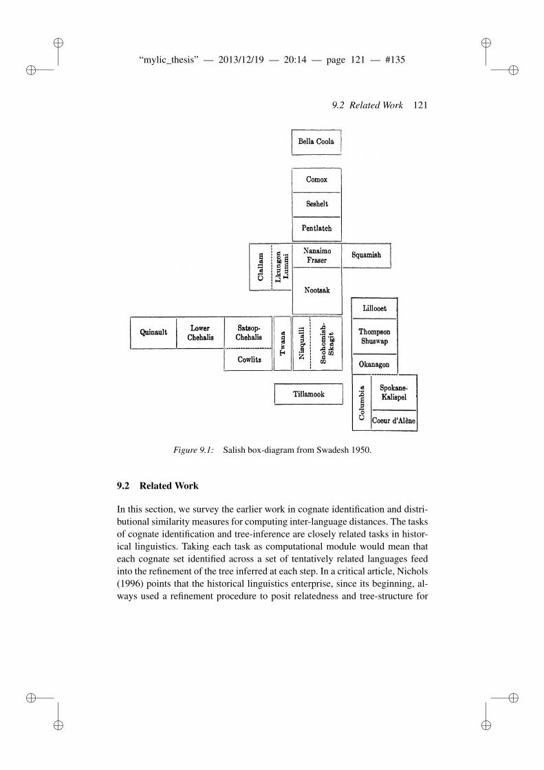
ii


ii

ii

9.2 Related Work 121

Figure 9.1: Salish box-diagram from Swadesh 1950.

9.2 Related Work

In this section, we survey the earlier work in cognate identification and distri-butional similarity measures for computing inter-language distances. The tasksof cognate identification and tree-inference are closely related tasks in histor-ical linguistics. Taking each task as computational module would mean thateach cognate set identified across a set of tentatively related languages feedinto the refinement of the tree inferred at each step. In a critical article, Nichols(1996) points that the historical linguistics enterprise, since its beginning, al-ways used a refinement procedure to posit relatedness and tree-structure for

ii


ii

ii


a set of tentatively related languages.48 The inter-language distance approachto tree-building, is incidentally straight-forward and comparably accurate incomparison to the computationally intensive Bayesian-based tree-inference ap-proach of Greenhill and Gray 2009.

The inter-language distances are either an aggregate score of the pair-wiseitem distances or based on a distributional similarity score. The string simi-larity measures used for the task of cognate identification can also be used forcomputing the similarity between two lexical items for a particular word sense.

9.2.1 Cognate identification

The task of identifying the genetically related words – cognates – is very wellexplored in computational linguistics. Kondrak (2002a) compares a numberof algorithms based on phonetic and orthographical similarity for judging thecognateness of a word pair. His work surveys string similarity / distance mea-sures such as edit distance, dice coefficient and longest common subsequenceratio (LCSR) for the task of cognate identification.

He developed a string matching algorithm based on articulatory features(called ALINE) for computing the similarity of a word pair. Although the algo-rithm is linguistically sound, it requires a International Phonetic transcription(IPA) transcribed input. ALINE was further evaluated against machine learn-ing algorithms such as Dynamic Bayesian Networks and Pair-wise HMMs forautomatic cognate identification (Kondrak and Sherif 2006). Even though, theapproach is technically sound, it suffers due to the bare-boned phonetic tran-scription used in Dyen, Kruskal and Black’s Indo-European dataset.49

Inkpen, Frunza and Kondrak (2005) compared various string similarity mea-sures for the task of automatic cognate identification for two closely relatedlanguages: English and French. The paper shows an impressive array of stringsimilarity measures. However, the results are too language specific to be gen-eralized for the rest of Indo-European family.

In another work, Ellison and Kirby (2006) use Scaled Edit Distance (SED)50

for computing intra-lexical similarity for estimating language distances basedon the dataset of Indo-European languages prepared by Dyen, Kruskal and

48This idea is quite similar to the famous paradigm of Expectation-Maximization in machinelearning field. Kondrak (2002b) uses this paradigm for extracting sound correspondences frompair-wise word lists for the task of cognate identification. The recent paper of Bouchard-Côtéet al. (2013) employs a feed-back procedure for the reconstruction of Proto-Austronesian witha great success.

49Available on http://www.wordgumbo.com/ie/cmp/index.htm.50SED for a pair of strings is defined as the edit distance normalized by the average of the

lengths of the pair of strings.

ii


ii

ii

9.2 Related Work 123

Black (1992). The distance matrix is then given as input to the NJ algorithmas implemented in PHYLIP package (Felsenstein 2002) to infer a tree for 87languages of Indo-European family.

Petroni and Serva (2010) use a modified version of Levenshtein distancefor inferring the trees of Indo-European and Austronesian language families.LD is usually normalized by the maximum of the lengths of the two wordsto account for length-bias. The normalized LD (LDN) can then be used incomputing distances between pairs of languages.

There are at least two ways of computing inter-language distances: LDNand LDND. Only pairs of words occupying the same slot in two lists are com-pared, i.e., words expressing the same sense in the two languages. LDN fortwo languages is computed as the mean of the normalized LD of all comparedword pairs. To compensate for chance similarity, LDN is further normalizedby the mean of all N(N− 1)/2 words to yield LDND, employed by Holmanet al. (2008a) for automatic language classification.

Petroni and Serva (2010) claim that LDN is more suitable than LDND formeasuring linguistic distances. In reply, Wichmann et al. (2010a) empiricallyshow that LDND performs better than LDN for distinguishing the languagesbelonging to a same family from the languages of other families. LDND wasdesigned to make sure that the chance resemblance, similarity in the phonemicinventory between unrelated languages do not influence the distance betweenthem.

9.2.2 Distributional measures

Huffman (1998) compute pair-wise language distances based on character n-grams extracted from Bible texts in European and American Indian languages(mostly from the Mayan language family). Singh and Surana (2007) use char-acter n-grams extracted from raw comparable corpora of ten languages fromthe Indian subcontinent for computing the pair-wise language distances be-tween languages belonging to two different language families (Indo-Aryanand Dravidian). Rama and Singh (2009) introduce a factored language modelbased on articulatory features to induce a articulatory feature level n-grammodel from the dataset of Singh and Surana 2007. The feature n-grams ofeach language pair are compared using distributional similarity measures suchas cross-entropy to yield a single point distance between a language pair.

Taking cue from the development of tree similarity measures in computa-tional biology, Pompei, Loreto and Tria (2011) evaluate the performance ofLDN vs. LDND on the ASJP and Austronesian Basic Vocabulary databases(Greenhill, Blust and Gray 2008). These authors compute NJ and Minimum

ii


ii

ii


Evolution trees51 for LDN as well as LDND distance matrices. They comparethe inferred trees to the classification given in Ethnologue (Lewis 2009) usingtwo different tree similarity measures: Generalized Robinson-Fould’s distance(GRF; A generalized version of Robinson-Fould’s [RF] distance) and Gener-alized Quartet distance (GQD). GRF and GQD are specifically designed toaccount for the polytomous nature – a node having more than two children –of the Ethnologue trees. Finally, Huff and Lonsdale (2011) compare the NJtrees from ALINE and LDND distance metrics to Ethnologue trees using RFdistance. The authors did not find any significant improvement by using a lin-guistically well-informed ALINE over LDND.

However, LD is only one of a number of string similarity measures used infields such as language technology, information retrieval and bio-informatics.Beyond the works cited above, so far there has to our knowledge been nostudy to compare different string similarity measures on the same dataset in or-der to determine their relative suitability for linguistic classification.52 In thispaper we compare various string similarity measures53 for the task of auto-matic language classification. We evaluate their effectiveness through distinc-tiveness measure and comparing them to the language classifications providedin WALS (World Atlas of Language Structures; Haspelmath et al. 2011) andEthnologue.

9.3 Contributions

In this article, we ask the following questions:

• Out of the numerous string similarity measures given in section 9.5:

– Which is the best suited for the tasks of distinguishing related lanu-gages from unrelated languages?

– Which is the best suited for the task of internal language classifi-cation?

– Is there a statistical procedure for determining the best string sim-ilarity measure?

• What is the best way to length normalize a string similarity measure?54

51A tree building algorithm closely related to NJ.52One reason for this may be that the experiments are computationally demanding, requiring

several days for computing a single measure over the whole ASJP dataset.53A complete list of string similarity measures is available on: http://www.coli.

uni-saarland.de/courses/LT1/2011/slides/stringmetrics.pdf54Marzal and Vidal (1993) propose an alternate normalization based on the length of the

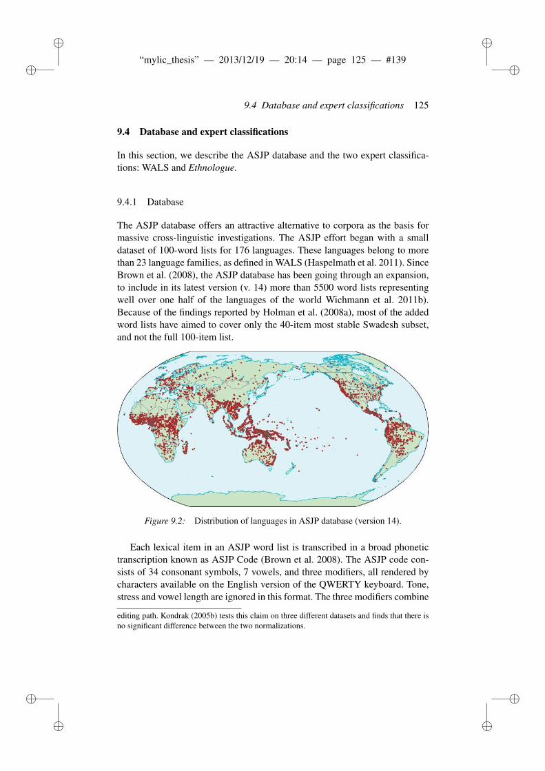
ii


ii

ii

9.4 Database and expert classifications 125

9.4 Database and expert classifications

In this section, we describe the ASJP database and the two expert classifica-tions: WALS and Ethnologue.

9.4.1 Database

The ASJP database offers an attractive alternative to corpora as the basis formassive cross-linguistic investigations. The ASJP effort began with a smalldataset of 100-word lists for 176 languages. These languages belong to morethan 23 language families, as defined in WALS (Haspelmath et al. 2011). SinceBrown et al. (2008), the ASJP database has been going through an expansion,to include in its latest version (v. 14) more than 5500 word lists representingwell over one half of the languages of the world Wichmann et al. 2011b).Because of the findings reported by Holman et al. (2008a), most of the addedword lists have aimed to cover only the 40-item most stable Swadesh subset,and not the full 100-item list.

Figure 9.2: Distribution of languages in ASJP database (version 14).

Each lexical item in an ASJP word list is transcribed in a broad phonetictranscription known as ASJP Code (Brown et al. 2008). The ASJP code con-sists of 34 consonant symbols, 7 vowels, and three modifiers, all rendered bycharacters available on the English version of the QWERTY keyboard. Tone,stress and vowel length are ignored in this format. The three modifiers combine

editing path. Kondrak (2005b) tests this claim on three different datasets and finds that there isno significant difference between the two normalizations.

ii


ii

ii


symbols to form phonologically complex segments (e.g., aspirated, glottalized,or nasalized segments).

In order to ascertain that our results would be comparable to those pub-lished by the ASJP group, we successfully replicated their experiments forLDN and LDND measures using the ASJP program and the ASJP dataset ver-sion 12 (Wichmann et al. 2010c).55 This database comprises of reduced (40–item) Swadesh lists for 4169 word lists. All pidgins, creoles, mixed languages,artificial languages, proto-languages and languages extinct before 1700 CEwere excluded for the experiment, as were language families represented byless than 10 word lists. This leaves a dataset with 3730 word lists. It turned outthat 60 word lists did not have English glosses for the items, which meant thatthey could not be processed by the program, so these languages were excludedfrom the analysis.

All the experiments reported in this paper were performed on a subset ofversion 14 of the ASJP database whose distribution is shown in figure 9.2.56

The database has 5500 word lists, including not only living languages, butalso extinct ones. The database also contains word lists for pidgins, creoles,mixed languages, artificial languages, and proto-languages, all of which havebeen excluded from the current study. Among the extinct languages, only thoselanguages were included which have gone extinct less than three centuries ago.Also, any word list containing less than 28 words (70%) was not included inthe final dataset. We use the family names of the WALS (Haspelmath et al.2011) classification. Following Wichmann et al. 2010a, any family with lessthan ten languages is excluded from our experiments. The final dataset for ourexperiments has 4743 word lists for 50 language families.

WALS. WALS classification is a two-level classification where each lan-guage belongs to a genus as well as family. A genus is a genetic classifica-tion unit given by Dryer (2000) and consists of set of languages supposedlydescended from a common ancestor which is 3000 to 3500 years old. For in-stance, Indic languages are classified as a separate genus from Iranian lan-guages although, it is quite well known that both Indic and Iranian languagesshare a common proto-Indo-Iranian ancestor.

Ethnologue. Ethnologue classification is a multi-level tree classification fora language family. Ethnologue classification was originally given by mission-aries and is very opportunistic in the inclusion of languages or genetic related-ness. The highest node in a family tree is the family itself and languages formthe lowest node. A internal node in the tree is not necessarily binary and can

55The original python program was kindly provided by Søren Wichmann. We modified theprogram to handle the ASJP modifiers.

56Available on http://email.eva.mpg.de/~wichmann/listss14.zip.

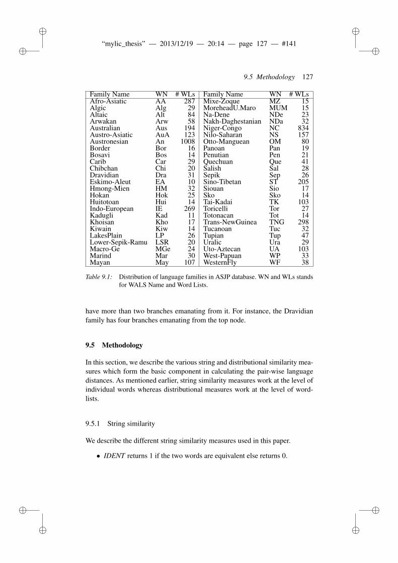
ii


ii

ii

9.5 Methodology 127

Family Name WN # WLs Family Name WN # WLsAfro-Asiatic AA 287 Mixe-Zoque MZ 15Algic Alg 29 MoreheadU.Maro MUM 15Altaic Alt 84 Na-Dene NDe 23Arwakan Arw 58 Nakh-Daghestanian NDa 32Australian Aus 194 Niger-Congo NC 834Austro-Asiatic AuA 123 Nilo-Saharan NS 157Austronesian An 1008 Otto-Manguean OM 80Border Bor 16 Panoan Pan 19Bosavi Bos 14 Penutian Pen 21Carib Car 29 Quechuan Que 41Chibchan Chi 20 Salish Sal 28Dravidian Dra 31 Sepik Sep 26Eskimo-Aleut EA 10 Sino-Tibetan ST 205Hmong-Mien HM 32 Siouan Sio 17Hokan Hok 25 Sko Sko 14Huitotoan Hui 14 Tai-Kadai TK 103Indo-European IE 269 Toricelli Tor 27Kadugli Kad 11 Totonacan Tot 14Khoisan Kho 17 Trans-NewGuinea TNG 298Kiwain Kiw 14 Tucanoan Tuc 32LakesPlain LP 26 Tupian Tup 47Lower-Sepik-Ramu LSR 20 Uralic Ura 29Macro-Ge MGe 24 Uto-Aztecan UA 103Marind Mar 30 West-Papuan WP 33Mayan May 107 WesternFly WF 38

Table 9.1: Distribution of language families in ASJP database. WN and WLs standsfor WALS Name and Word Lists.

have more than two branches emanating from it. For instance, the Dravidianfamily has four branches emanating from the top node.

9.5 Methodology

In this section, we describe the various string and distributional similarity mea-sures which form the basic component in calculating the pair-wise languagedistances. As mentioned earlier, string similarity measures work at the level ofindividual words whereas distributional measures work at the level of word-lists.

9.5.1 String similarity

We describe the different string similarity measures used in this paper.

• IDENT returns 1 if the two words are equivalent else returns 0.

ii


ii

ii


• PREFIX returns the length of the common prefix divided by the lengthof the longer word.

• DICE is defined as the number of shared segment bigrams divided bythe total number of bigrams in both the words.

• LCSR is defined as the length of the longest common subsequence di-vided by the length of the longer word.

• TRIGRAM is defined as twice the number of shared trigrams divided bythe sum of the shared trigrams.

• XDICE is defined similar to DICE where a bigram is a trigram with themiddle letter removed.

• Jaccard’s index, JCD, is a set cardinality measure. It is defined as theratio of the cardinality of the intersection of the bigrams between thetwo words to the cardinality of the union of the sets of bigrams betweentwo words.

Each Msim is converted to its distance counterpart by subtracting the scorefrom 1.0. Lin (1998) investigates three distance to similarity conversion tech-niques and motivates the results from an information-theoretical point. In thisarticle, we do not investigate this rather, we stick to the traditional conversiontechnique. Note that this conversion can sometimes result in a negative dis-tance which is due to the double normalization involved in LDND. A suffix“D” is added to each measure to indicate the LDND variant.

9.5.2 N-gram similarity

This section describes the distributional similarity measures originally devel-oped for automatic language identification in a multi-lingual document. Thisline of work started with the heavily cited paper of Cavnar and Trenkle 1994who use character n-grams for text categorization. They observe that the fre-quency of character n-grams for a particular document category follows a Zip-fian distribution. The rank of character n-grams vary for different categoriesand documents belonging to the same category have similar Zipfian distribu-tions. Based on this idea, Dunning (1994) postulates that the character n-gramsfor a language has its own signature distribution. Comparing the signatures oftwo languages can yield a single point distance between the languages undercomparison. The comparison procedure is usually accomplished through theuse of a distributional similarity measure (Singh 2006). The following stepsare followed for extracting the phoneme n-gram profile for a language.

ii


ii

ii

9.5 Methodology 129

For a language, the n-gram extraction procedure is as follows:

• A n-gram is defined as the consecutive phonemes in a window of N. Thevalue of N usually ranges from 3 to 5.

• All the unigrams, bigrams and trigrams are extracted for a lexical item.This step is repeated for all the lexical items in a word list.

• All the extracted n-grams are mixed and sorted in the descending orderof their frequency. The relative frequency of the n-grams are computed.

• Only the top G n-grams are retained and the rest of them are pruned.Usually G is fixed at 50.

For every pair of language, the n-gram profiles are compared using Out-of-Rank measure, Jaccard’s index, Dice distance, Overlap distance, Manhattandistance and Euclidean distance. The distances are explained below:

1. Out-of-Rank measure is defined as the aggregate sum of the absolutedifference in the rank of the shared n-grams between a pair of language.

2. Jaccard’s index is a set cardinality measure. It is defined as the ratioof the cardinality of the intersection of the n-grams between the twolanguages to the cardinality of the union of the two languages.

3. Dice distance is related to Jaccard’s Index. It is defined as the ratio oftwice the number of shared n-grams to the total number of n-grams inboth the language profiles.

4. Manhattan distance is defined as the sum of the absolute difference be-tween the relative frequency of the shared n-grams.

5. Euclidean distance is defined in a similar fashion to Manhattan distancewhere the individual terms are squared.

One possible set of measures, based on n-grams, and could be included areinformation theoretic based such as cross entropy and KL-divergence. Thesemeasures have been well-studied in natural language processing systems suchas machine translation, natural language parsing, sentiment identification, andalso in automatic language identification. The probability distributions requiredfor using these measures are usually estimated through maximum likelihoodestimation which require a fairly large amount of data. While replicating theoriginal ASJP experiments on the version 12 ASJP database, we tested if theabove distributional measures, [1–4] perform as well as LDN. Unfortunately,

ii


ii

ii


the results are on the discouraging side of the spectrum and we do not repeatthe experiments on the version 14 of the database. One main reason for this re-sult is the relatively small size of ASJP word list. The relatively small word listsize provides a poor estimates of the true language signatures. The next sectiondescribes the three different evaluation measures for comparing the differentstring similarity measures.

9.6 Evaluation measures

In this section, we describe the three different evaluation measures for rankingthe string similarity measures given in section 9.5.

1. The first measure dist, originally given by Wichmann et al. (2010a) totest if LDND performs better than LDN in the task of distinguishingrelated languages from unrelated languages.

2. The second measure, RW, is a special case of pearson’s r – called pointbiserial correlation (Tate 1954) – for computing the agreement betweenWALS’s two-level classification and the intra-family pair-wise distances.

3. The third measure, γ , is related to the Goodman and Kruskal’s Gamma(1954) which measures the strength of association between two ordinalvariables. In this paper, it is used to compute the level of agreementbetween the Ethnologue classification and the pair-wise intra-languagedistances.

9.6.1 Dist

Initially, we define a function f am which takes a language name and returnsthe family to which the language belongs.

When, f am(i) = f am( j)

din =1

∑i= j 1 ∑i 6= j

di, j (9)

When, f am(i) 6= f am( j)

dout =1

∑i6= j 1 ∑i6= j

di, j (10)

sdout = stdev(di, j) (11)

ii


ii

ii

9.6 Evaluation measures 131

dist =din−dout

sdout(12)

The dist measure for a family consists of two components: the pair-wisedistances inside a family (din) and the pair-wise distances from each languagein the family to the rest of the language families. A comparatively higher distvalue suggests that a measure is particularly resistant to random similarities be-tween unrelated languages and performs well at distinguishing elements froma genealogical unit from the rest of the dataset. The resistance of a string sim-ilarity measure to other language families is reflected by the value of sdout

which denotes the standard deviation of dout .

9.6.2 Correlation with WALS

The WALS database has classification at three levels. The top level is the fam-ily of the language, second level is the genus and the lowest level is the lan-guage itself. Two languages from different genera and same family have a dis-tance of 2 and a distance of 1 if they are in the same genus. This allows us todefine a inter-language distance matrix between the languages in a family. TheWALS distance matrix can be compared to the distance matrices of any mea-sure using Pearson’s r. The families with a single genus have no correlationand the corresponding row is left blank.

9.6.3 Agreement with Ethnologue

Given a pair-wise distance-matrix d of size N×N, where each cell di j is thedistance between two languages i and j and an Ethnologue tree E, the compu-tation of γ for a language family is defined as follows:

1. Find all the triplets for a language family of size N. A triplet, t for a lan-guage family is defined as {i, j,k}, where i, j,k are languages belongingto a family. A language family of size N has

(N3

)triplets.

2. For the members of each such triplet t, there are three distances di j, dik,and d jk. The expert classification tree E can treat the three languages{i, j,k} in four possible ways (| denotes a partition): {i, j | k}, {i,k | j},{ j,k | i} or can have a tie where all languages emanate from the samenode. All ties are ignored in the computation of γ .

ii


ii

ii


3. For a partition {i, j | k}, the distance matrix d is said to agree completelywhen the following conditions are satisfied:

di j < dik (13)

di j < d jk (14)

A triplet that satisfies these conditions is counted as a concordant com-parison, C; else it is counted as disconcordant comparison, D.

4. Steps 2 and 3 are repeated for all the(N

3

)triplets to yield γ for a family

defined as γ = C−DC+D .

At this point, one might wonder about the decision for not using a off-the-shelf tree-building algorithm to infer a tree and compare the resulting tree withthe Ethnologue classification. Although both the works of Pompei, Loreto andTria 2011; Huff and Lonsdale 2011 compare their trees to Ethnologue usingcleverly crafted tree-distance measures, they do not compare their distance ma-trices directly. A direct comparison of a family distance matrix to the family’sEthnologue tree removes the errors induced by the tree inference algorithm.The results of Wichmann et al. 2011a, suggest that the GE measure shows ahigh negative correlation with the GRF and GQD for the LDND distance ma-trix computed from ASJP database (v. 14) families.

9.7 Item-item vs. length visualizations

A distance measure such as LDND has two components:

• The average LDN computed between pair-wise lexical items for thesame meaning.

• The average LDN computed between pair-wise lexical items for differ-ent meaning-meaning pair.

Although, there have been multitude of publications involving LDND, noeffort has been put to look the base components of LDND through a magni-fying glass. It is quite interesting to see the overall distribution between LDand the lengths of the lexical items under comparison. We proceed to seethe variation of the pair-wise LDs vs. the pair-wise word lengths for lexicalitems sharing the same meaning and different meanings. We select a small (31word lists) but well-studied language family called Dravidian family, spokenin South Asia (comprising of modern day India, Pakistan, and Nepal), for thisstudy.

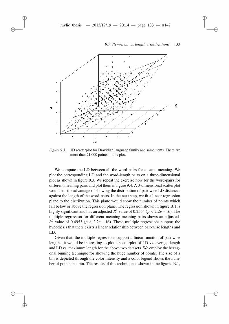
ii


ii

ii

9.7 Item-item vs. length visualizations 133

Figure 9.3: 3D scatterplot for Dravidian language family and same items. There aremore than 21,000 points in this plot.

We compute the LD between all the word pairs for a same meaning. Weplot the corresponding LD and the word-length pairs on a three-dimensionalplot as shown in figure 9.3. We repeat the exercise now for the word-pairs fordifferent meaning pairs and plot them in figure 9.4. A 3-dimensional scatterplotwould has the advantage of showing the distribution of pair-wise LD distancesagainst the length of the word-pairs. In the next step, we fit a linear regressionplane to the distribution. This plane would show the number of points whichfall below or above the regression plane. The regression shown in figure B.1 ishighly significant and has an adjusted-R2 value of 0.2554 (p < 2.2e−16). Themultiple regression for different meaning-meaning pairs shows an adjusted-R2 value of 0.4953 (p < 2.2e− 16). These multiple regressions support thehypothesis that there exists a linear relationship between pair-wise lengths andLD.

Given that, the multiple regressions support a linear function of pair-wiselengths, it would be interesting to plot a scatterplot of LD vs. average lengthand LD vs. maximum length for the above two datasets. We employ the hexag-onal binning technique for showing the huge number of points. The size of abin is depicted through the color intensity and a color legend shows the num-ber of points in a bin. The results of this technique is shown in the figures B.1,

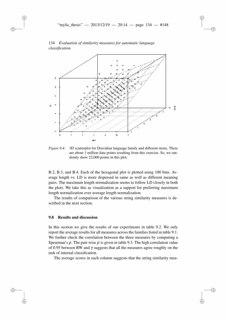
ii


ii

ii


Figure 9.4: 3D scatterplot for Dravidian language family and different items. Thereare about 1 million data points resulting from this exercise. So, we ran-domly show 22,000 points in this plot.

B.2, B.3, and B.4. Each of the hexagonal plot is plotted using 100 bins. Av-erage length vs. LD is more dispersed in same as well as different meaningpairs. The maximum length normalization seems to follow LD closely in boththe plots. We take this as visualization as a support for preferring maximumlength normalization over average length normalization.

The results of comparison of the various string similarity measures is de-scribed in the next section.


In this section we give the results of our experiments in table 9.2. We onlyreport the average results for all measures across the families listed in table 9.1.We further check the correlation between the three measures by computing aSpearman’s ρ . The pair-wise ρ is given in table 9.3. The high correlation valueof 0.95 between RW and γ suggests that all the measures agree roughly on thetask of internal classification.

The average scores in each column suggests that the string similarity mea-

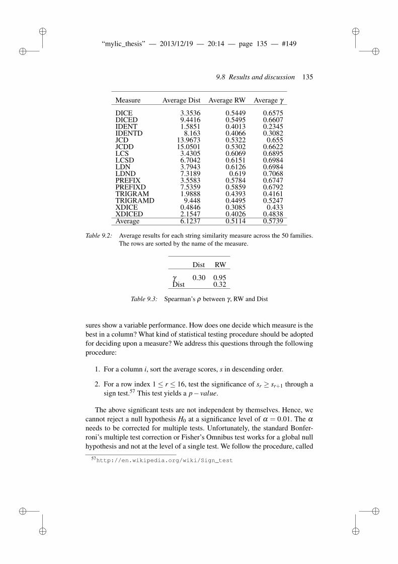
ii


ii

ii


Measure Average Dist Average RW Average γ

DICE 3.3536 0.5449 0.6575DICED 9.4416 0.5495 0.6607IDENT 1.5851 0.4013 0.2345IDENTD 8.163 0.4066 0.3082JCD 13.9673 0.5322 0.655JCDD 15.0501 0.5302 0.6622LCS 3.4305 0.6069 0.6895LCSD 6.7042 0.6151 0.6984LDN 3.7943 0.6126 0.6984LDND 7.3189 0.619 0.7068PREFIX 3.5583 0.5784 0.6747PREFIXD 7.5359 0.5859 0.6792TRIGRAM 1.9888 0.4393 0.4161TRIGRAMD 9.448 0.4495 0.5247XDICE 0.4846 0.3085 0.433XDICED 2.1547 0.4026 0.4838Average 6.1237 0.5114 0.5739

Table 9.2: Average results for each string similarity measure across the 50 families.The rows are sorted by the name of the measure.

Dist RW

γ 0.30 0.95Dist 0.32

Table 9.3: Spearman’s ρ between γ , RW and Dist

sures show a variable performance. How does one decide which measure is thebest in a column? What kind of statistical testing procedure should be adoptedfor deciding upon a measure? We address this questions through the followingprocedure:

1. For a column i, sort the average scores, s in descending order.

2. For a row index 1 ≤ r ≤ 16, test the significance of sr ≥ sr+1 through asign test.57 This test yields a p− value.

The above significant tests are not independent by themselves. Hence, wecannot reject a null hypothesis H0 at a significance level of α = 0.01. The α

needs to be corrected for multiple tests. Unfortunately, the standard Bonfer-roni’s multiple test correction or Fisher’s Omnibus test works for a global nullhypothesis and not at the level of a single test. We follow the procedure, called

57http://en.wikipedia.org/wiki/Sign_test

ii


ii

ii


False Discovery Rate (FDR), given by Benjamini and Hochberg (1995) foradjusting the α value for multiple tests. Given H1 . . .Hm null hypotheses andP1 . . .Pm p-values, the procedure works as follows:

1. Sort the Pk, 1 ≤ k ≤ m, values in ascending order. k is the rank of ap-value.

2. The adjusted α∗k value for Pk is km α .

3. Reject all the H0s from 1, . . . ,k where Pk+1 > α∗k .

The above procedure ensures that the chance of incorrectly rejecting a null hy-pothesis is 1 in 20 for α = 0.05 and 1 in 100 for α = 0.01. In this experimentalcontext, this suggests that we erroneously reject 0.75 true null hypotheses outof 15 hypotheses for α = 0.05 and 0.15 hypotheses for α = 0.01. We reportthe γ , Dist and RW for each family in tables B.1, B.2, and B.3. In each of thesetables, only those measures which are above the average scores, from table 9.2,are reported. A empty row in table B.1 implies that all triplets in Ethnologuetree are ties and; in table B.3, implies that there is a single genus in that family.

The FDR procedure for γ suggests that no sign test is significant. This isin agreement with the result of Wichmann et al. 2010a who showed that thechoice of LDN or LDND is quite unimportant for the task of internal clas-sification. The FDR procedure for RW suggests that LDN > LCS, LCS >PREFIXD, DICE > JCD, and JCD > JCDD. Here A > B denotes that A issignificantly better than B. The FDR procedure for Dist suggests that JCDD >JCD, JCD > TRID, DICED > IDENTD, LDND > LCSD, and LCSD > LDN.

The results point towards an important direction in the task of buildingcomputational systems for automatic language classification. The pipeline forsuch a system consists of 1) distinguishing related languages from unrelatedlanguages and 2) internal classification accuracy. JCDD performs the best withrespect to Dist. Further, JCDD is derived from JCD and can be computed inO(m+n), for two strings of length m and n. In comparison, LDN is in the orderof O(mn). In general, the computational complexity for computing distancebetween two word lists for all the significant measures is given in table 9.4.Based on the computational complexity and the significance scores, we pro-pose that JCDD be used for step 1 and measure like LDN be used for internalclassification.

9.9 Conclusion

We conclude the article by pointing that this is the first known attempt at ap-plying more than 20 similarity measures for more than half of the world’s lan-

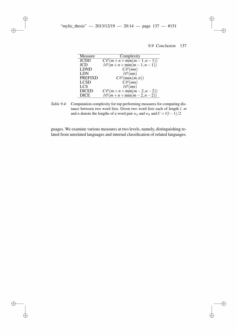
ii


ii

ii

9.9 Conclusion 137

Measure ComplexityJCDD CO(m+n+min(m−1,n−1))JCD lO(m+n+min(m−1,n−1))LDND CO(mn)LDN lO(mn)PREFIXD CO(max(m,n))LCSD CO(mn)LCS lO(mn)DICED CO(m+n+min(m−2,n−2))DICE lO(m+n+min(m−2,n−2))

Table 9.4: Computation complexity for top performing measures for computing dis-tance between two word lists. Given two word lists each of length l. mand n denote the lengths of a word pair wa and wb and C = l(l−1)/2

guages. We examine various measures at two levels, namely, distinguishing re-lated from unrelated languages and internal classification of related languages.

ii


ii

ii

ii


ii

ii

REFERENCES

Abney, Steven 2004. Understanding the Yarowsky algorithm. ComputationalLinguistics 30 (3): 365–395.

Abney, Steven 2010. Semisupervised learning for computational linguistics.Chapman & Hall/CRC.

Abney, Steven and Steven Bird 2010. The human language project: Buildinga universal corpus of the world’s languages. Proceedings of the 48thmeeting of the ACL, 88–97. Uppsala: ACL.

Adesam, Yvonne, Malin Ahlberg and Gerlof Bouma 2012. bokstaffua, bok-staffwa, bokstafwa, bokstaua, bokstawa... Towards lexical link-up for acorpus of Old Swedish. Proceedings of KONVENS, 365–369.

Agarwal, Abhaya and Jason Adams 2007. Cognate identification and phylo-genetic inference: Search for a better past. Technical Report, CarnegieMellon University.

Anttila, Raimo 1989. Historical and comparative linguistics. Volume 6 ofCurrent Issues in Linguistic Theory. Amsterdam/Philadelphia: John Ben-jamins Publishing Company.

Atkinson, Quentin D. 2011. Phonemic diversity supports a serial founder effectmodel of language expansion from Africa. Science 332 (6027): 346.

Atkinson, Quentin D. and Russell D. Gray 2005. Curious parallels and curiousconnections—phylogenetic thinking in biology and historical linguistics.Systematic Biology 54 (4): 513–526.

Atkinson, Quentin D. and Russell D. Gray 2006. How old is the Indo-Europeanlanguage family? Progress or more moths to the flame. Peter Forster andCollin Renfrew (eds), Phylogenetic methods and the prehistory of lan-guages, 91–109. Cambridge: The McDonald Institute for ArchaelogicalResearch.

Bakker, Dik, André Müller, Viveka Velupillai, Søren Wichmann, Cecil H.Brown, Pamela Brown, Dmitry Egorov, Robert Mailhammer, AnthonyGrant and Eric W. Holman 2009. Adding typology to lexicostatistics:A combined approach to language classification. Linguistic Typology 13(1): 169–181.

Beekes, Robert Stephen Paul 1995. Comparative Indo-European linguistics:

ii


ii

ii

140 References

An introduction. Amsterdam and Philadelphia: John Benjamins Publish-ing Company.

Benjamini, Yoav and Yosef Hochberg 1995. Controlling the false discoveryrate: A practical and powerful approach to multiple testing. Journal ofthe Royal Statistical Society. Series B (Methodological) 57 (1): 289–300.

Bergsland, Knut and Hans Vogt 1962. On the validity of glottochronology.Current Anthropology 3 (2): 115–153.

Bergsma, Shane and Grzegorz Kondrak 2007. Alignment-based discriminativestring similarity. Proceedings of the 45th annual meeting of the associ-ation of computational linguistics, 656–663. Prague, Czech Republic:Association for Computational Linguistics.

Bickel, Balthasar 2002. The AUTOTYP research program. Invited talk given atthe Annual Meeting of the Linguistic Typology Resource Center Utrecht.

Bickel, Balthasar and Johanna Nichols 2002. Autotypologizing databases andtheir use in fieldwork. Proceedings of the LREC 2002 workshop on re-sources and tools in field linguistics.

Birch, Alexandra, Miles Osborne and Philipp Koehn 2008. Predicting successin machine translation. Proceedings of the 2008 conference on empiricalmethods in natural language processing, 745–754. Honolulu, Hawaii:Association for Computational Linguistics.

Bloomfield, Leonard 1935. Language. London: Allen, George and Unwin.Borin, Lars 1988. A computer model of sound change: An example from Old

Church Slavic. Literary and Linguistic Computing 3 (2): 105–108.Borin, Lars 2009. Linguistic diversity in the information society. Proceedings

of the SALTMIL 2009 workshop on information retrieval and informationextraction for less resourced languages, 1–7. Donostia: SALTMIL.

Borin, Lars 2012. Core vocabulary: A useful but mystical concept in somekinds of linguistics. Shall we play the festschrift game? Essays on theoccasion of Lauri Carlson’s 60th birthday, 53–65. Berlin: Springer.

Borin, Lars 2013a. For better or for worse? Going beyond short word listsin computational studies of language diversity. Presented at LanguageDiversity Congress, Groningen.

Borin, Lars 2013b. The why and how of measuring linguistic differences.Lars Borin and Anju Saxena (eds), Approaches to measuring linguisticdifferences, 3–26. Berlin: De Gruyter Mouton.

Borin, Lars, Bernard Comrie and Anju Saxena 2013. The intercontinental dic-tionary series – a rich and principled database for language comparison.Lars Borin and Anju Saxena (eds), Approaches to measuring linguisticdifferences, 285–302. Berlin: De Gruyter Mouton.

ii


ii

ii

References 141

Borin, Lars, Devdatt Dubhashi, Markus Forsberg, Richard Johansson, Dim-itrios Kokkinakis and Pierre Nugues 2013. Mining semantics for cultur-omics: towards a knowledge-based approach. Proceedings of the 2013international workshop on Mining unstructured big data using naturallanguage processing, 3–10. Association for Computing Machinery.

Borin, Lars and Anju Saxena (eds) 2013. Approaches to measuring linguisticdifferences. Berlin: De Gruyter Mouton.

Bouchard-Côté, Alexandre, David Hall, Thomas L. Griffiths and Dan Klein2013. Automated reconstruction of ancient languages using probabilis-tic models of sound change. Proceedings of the National Academy ofSciences 110 (11): 4224–4229.

Bouchard-Côté, Alexandre, Percy Liang, Thomas L. Griffiths and Dan Klein2007. A probabilistic approach to diachronic phonology. Empirical meth-ods in natural language processing.

Bouckaert, Remco, Philippe Lemey, Michael Dunn, Simon J. Greenhill,Alexander V. Alekseyenko, Alexei J. Drummond, Russell D. Gray,Marc A. Suchard and Quentin D. Atkinson 2012. Mapping the originsand expansion of the Indo-European language family. Science 337 (6097):957–960.

Brew, Chris and David McKelvie 1996. Word-pair extraction for lexicography.Proceedings of the second international conference on new methods inlanguage processing, 45–55. Ankara.

Briscoe, Edward J. (ed.) 2002. Linguistic evolution through language acquisi-tion. Cambridge: Cambridge University Press.

Brown, Cecil H., Eric W. Holman and Søren Wichmann 2013. Sound corre-spondences in the world’s languages. Language 89 (1): 4–29.

Brown, Cecil H., Eric W. Holman, Søren Wichmann and Viveka Velupillai2008. Automated classification of the world’s languages: A descriptionof the method and preliminary results. Sprachtypologie und Universalien-forschung 61 (4): 285–308.

Burrow, Thomas H. and Murray B. Emeneau 1984. A Dravidian etymologicaldictionary (rev.). Oxford: Clarendon Press.

Campbell, Lyle 2003. How to show languages are related: Methods for dis-tant genetic relationship. Brian D. Joseph and Richard D. Janda (eds),The handbook of historical linguistics, 262–282. Oxford, UK: BlackwellPublishing.

Campbell, Lyle 2004. Historical linguistics: An introduction. Edinburgh: Ed-inburgh University Press.

Campbell, Lyle 2012. Classification of the indigenous languages of South

ii


ii

ii

142 References

America. Lyle Campbell and Verónica Grondona (eds), The indigenouslanguages of South America, 59–166. Berlin: De Gruyter Mouton.

Campbell, Lyle and Mauricio J. Mixco 2007. A glossary of historical linguis-tics. University of Utah Press.

Campbell, Lyle and William J. Poser 2008. Language classification: Historyand method. Cambridge University Press.

Cavnar, William B. and John M. Trenkle 1994. N-gram-based text catego-rization. Proceedings of SDAIR-94, 3rd annual symposium on documentanalysis and information retrieval, 161–175. Las Vegas, US.

Chen, Matthew Y. and William S-Y. Wang 1975. Sound change: actuation andimplementation. Language 51: 255–281.

Collinge, Neville Edgar 1985. The laws of Indo-European. Volume 35. Ams-terdam/Philadelphia: John Benjamins Publishing Company.

Cooper, Martin C. 2008. Measuring the semantic distance between languagesfrom a statistical analysis of bilingual dictionaries. Journal of Quantita-tive Linguistics 15 (1): 1–33.

Covington, Michael A. 1996. An algorithm to align words for historical com-parison. Computational Linguistics 22 (4): 481–496.

Croft, William 2000. Explaining language change: An evolutionary approach.Pearson Education.

Croft, William 2008. Evolutionary linguistics. Annual Review of Anthropology37 (1): 219–234.

Crowley, Terry and Claire Bowern 2009. An introduction to historical linguis-tics. 4. USA: Oxford University Press.

Cysouw, Michael and Hagen Jung 2007. Cognate identification and alignmentusing practical orthographies. Proceedings of ninth meeting of the ACLspecial interest group in computational morphology and phonology, 109–116. Association for Computational Linguistics.

Damerau, Fred J. 1964. A technique for computer detection and correction ofspelling errors. Communications of the ACM 7 (3): 171–176.

Darwin, Charles 1871. The descent of man. London: Murray.Daume III, Hal 2009. Non-parametric Bayesian areal linguistics. Proceed-

ings of human language technologies: The 2009 annual conference of thenorth american chapter of the association for computational linguistics,593–601. Association for Computational Linguistics.

Dawkins, Richard 2006. The selfish gene. 2. New York: Oxford universitypress.

De Oliveira, Paulo Murilo Castro, Adriano O Sousa and Søren Wichmann

ii


ii

ii

References 143

2013. On the disintegration of (proto-) languages. International Jour-nal of the Sociology of Language 2013 (221): 11–19.

De Oliveira, Paulo Murilo Castro, Dietrich Stauffer, Søren Wichmann andSuzana Moss De Oliveira 2008. A computer simulation of language fam-ilies. Journal of Linguistics 44 (3): 659–675.

Dobson, Annette J., Joseph B. Kruskal, David Sankoff and Leonard J. Savage1972. The mathematics of glottochronology revisited. AnthropologicalLinguistics 14 (6): 205–212.

Dolgopolsky, Aron B. 1986. A probabilistic hypothesis concerning the oldestrelationships among the language families of northern Eurasia. Vitalij V.Shevoroshkin and Thomas L. Markey (eds), Typology, relationship, andtime: A collection of papers on language change and relationship by So-viet linguists, 27–50. Ann Arbor, MI: Karoma.

Donohue, Mark 2012. Typology and Areality. Language Dynamics andChange 2 (1): 98–116.

Donohue, Mark, Rebecca Hetherington, James McElvenny and Virginia Daw-son 2013. World phonotactics database. Department of Linguistics, TheAustralian National University. http://phonotactics.anu.edu.au.

Dryer, Matthew S. 2000. Counting genera vs. counting languages. LinguisticTypology 4: 334–350.

Dryer, Matthew S. 2011. Genealogical Language List.Dunn, Michael, Simon J. Greenhill, Stephen C. Levinson and Russell D. Gray

2011. Evolved structure of language shows lineage-specific trends inword-order universals. Nature 473 (7345): 79–82.

Dunn, Michael, Stephen C. Levinson and Eva Lindström 2008. Structuralphylogeny in historical linguistics: Methodological explorations appliedin island melanesia. Language 84 (4): 710–59.

Dunn, Michael, Angela Terrill, Ger Reesink, Robert A. Foley and Stephen C.Levinson 2005. Structural phylogenetics and the reconstruction of ancientlanguage history. Science 309 (5743): 2072–2075.

Dunning, Ted 1994. Statistical identification of language. Technical reportCRL MCCS-94-273, Computing Research Lab, New Mexico State Uni-versity.

Durbin, Richard, Sean R. Eddy, Anders Krogh and Graeme Mitchison 2002.Biological sequence analysis: Probabilistic models of proteins and nu-cleic acids. Cambridge: Cambridge University Press.

Durham, Stanton P. and David Ellis Rogers 1969. An application of computerprogramming to the reconstruction of a proto-language. Proceedings of

ii


ii

ii

144 References

the 1969 conference on computational linguistics, 1–21. Association forComputational Linguistics.

Durie, Mark and Malcolm Ross (eds) 1996. The comparative method re-viewed: regularity and irregularity in language change. USA: OxfordUniversity Press.

Dyen, Isidore, Joseph B. Kruskal and Paul Black 1992. An Indo-Europeanclassification: A lexicostatistical experiment. Transactions of the Ameri-can Philosophical Society 82 (5): 1–132.

Eger, Steffen 2013. Sequence alignment with arbitrary steps and further gen-eralizations, with applications to alignments in linguistics. InformationSciences 237 (July): 287–304.

Eger, Steffen and Ineta Sejane 2010. Computing semantic similarity frombilingual dictionaries. Proceedings of the 10th International Conferenceon the Statistical Analysis of Textual Data (JADT-2010), 1217–1225.

Ellegård, Alvar 1959. Statistical measurement of linguistic relationship. Lan-guage 35 (2): 131–156.

Ellison, T. Mark and Simon Kirby 2006. Measuring language divergence byintra-lexical comparison. Proceedings of the 21st international confer-ence on computational linguistics and 44th annual meeting of the associ-ation for computational linguistics, 273–280. Sydney, Australia: Associ-ation for Computational Linguistics.

Embleton, Sheila M. 1986. Statistics in historical linguistics. Volume 30.Brockmeyer.

Evans, Nicholas and Stephen C. Levinson 2009. The myth of language univer-sals: Language diversity and its importance for cognitive science. Behav-ioral and Brain Sciences 32: 429–492.

Evans, Steven N., Don Ringe and Tandy Warnow 2006. Inference of diver-gence times as a statistical inverse problem. Phylogenetic methods andthe prehistory of languages. McDonald institute monographs, 119–130.

Fellbaum, Christiane 1998. WordNet: An electronic database. Cambridge,Massachusetts: MIT Press.

Felsenstein, J. 1993. PHYLIP (phylogeny inference package) version 3.5 c.Department of Genetics, University of Washington, Seattle, vol. 1118.

Felsenstein, Joseph 2002. PHYLIP (phylogeny inference package) version 3.6a3. Distributed by the author. Department of Genome Sciences, Univer-sity of Washington, Seattle.

Felsenstein, Joseph 2004. Inferring phylogenies. Sunderland, Massachusetts:Sinauer Associates.

ii


ii

ii

References 145

Fortson, Benjamin W. 2003. An approach to semantic change. Brian D. Josephand Richard D. Janda (eds), The handbook of historical linguistics, 648–666. Wiley Online Library.

Fox, Anthony 1995. Linguistic reconstruction: An introduction to theory andmethod. Oxford University Press.

Garrett, Andrew 1999. A new model of Indo-European subgrouping and dis-persal. Steve S. Chang, Lily Liaw and Josef Ruppenhofer (eds), Pro-ceedings of the Twenty-Fifth Annual Meeting of the Berkeley LinguisticsSociety, 146–156. Berkeley: Berkeley Linguistic Society.

Georgi, Ryan, Fei Xia and William Lewis 2010. Comparing language similar-ity across genetic and typologically-based groupings. Proceedings of the23rd International Conference on Computational Linguistics, 385–393.Association for Computational Linguistics.

Gilij, Filippo Salvatore 2001. Saggio di storia americana, osia storia natu-rale, ciuile, e sacra de regni, e delle provincie spagnuole di terra-fermanell’america meridional/descrita dall’abate filippo salvadore gilij.-roma:per luigi perego erede salvioni..., 1780-1784. Textos clásicos sobre la his-toria de venezuela:[recopilación de libros digitalizados], 11. MAPFRE.

Goddard, Cliff 2001. Lexico-semantic universals: A critical overview. Lin-guistic Typology, pp. 1–65.

Goodman, Leo A. and William H. Kruskal 1954. Measures of association forcross classifications. Journal of the American Statistical Association, pp.732–764.

Graff, P., Z. Balewski, K. L. Evans, A. Mentzelopoulos, K. Snyder, E. Taliep,M. Tarczon, and X. Wang 2011. The World Lexicon (WOLEX) Corpus.http://www.wolex.org/.

Gravano, Luis, Panagiotis G. Ipeirotis, Hosagrahar Visvesvaraya Jagadish,Nick Koudas, Shanmugauelayut Muthukrishnan, Lauri Pietarinen and Di-vesh Srivastava 2001. Using q-grams in a DBMS for approximate stringprocessing. IEEE Data Engineering Bulletin 24 (4): 28–34.

Gray, Russell D. and Quentin D. Atkinson 2003. Language-tree divergencetimes support the Anatolian theory of Indo-European origin. Nature 426(6965): 435–439.

Gray, Russell D., David Bryant and Simon J. Greenhill 2010. On the shape andfabric of human history. Philosophical Transactions of the Royal SocietyB: Biological Sciences 365 (1559): 3923–3933.

Gray, Russell D. and Fiona M. Jordan 2000. Language trees support theexpress-train sequence of Austronesian expansion. Nature 405 (6790):1052–1055.

ii


ii

ii

146 References

Greenberg, Joseph H. 1993. Observations concerning Ringe’s “Calculating thefactor of chance in language comparison”. Proceedings of the AmericanPhilosophical Society 137 (1): 79–90.

Greenhill, Simon J., Robert Blust and Russell D. Gray 2008. The Austronesianbasic vocabulary database: from bioinformatics to lexomics. EvolutionaryBioinformatics Online 4: 271–283.

Greenhill, Simon J., Alexei J. Drummond and Russell D. Gray 2010. How ac-curate and robust are the phylogenetic estimates of Austronesian languagerelationships? PloS one 5 (3): e9573.

Greenhill, Simon J. and Russell D. Gray 2009. Austronesian languagephylogenies: Myths and misconceptions about Bayesian computationalmethods. Austronesian Historical Linguistics and Culture History: AFestschrift for Robert Blust, pp. 375–397.

Grimes, Joseph E. and Frederick B. Agard 1959. Linguistic divergence inRomance. Language 35 (4): 598–604.

Gulordava, Kristina and Marco Baroni 2011. A distributional similarity ap-proach to the detection of semantic change in the Google Books Ngramcorpus. Proceedings of the GEMS 2011 workshop on geometrical mod-els of natural language semantics, 67–71. Association for ComputationalLinguistics.

Gusfield, Dan 1997. Algorithms on strings, trees and sequences: computerscience and computational biology. Cambridge University Press.

Guy, Jacques B. M. 1994. An algorithm for identifying cognates in bilingualwordlists and its applicability to machine translation. Journal of Quanti-tative Linguistics 1 (1): 35–42.

Haas, Mary R. 1958. Algonkian-Ritwan: The end of a controversy. Interna-tional Journal of American Linguistics 24 (3): 159–173.

Hammarström, Harald 2009. Sampling and genealogical coverage in theWALS. Linguistic Typology 13 (1): 105–119. Plus 198pp appendix.

Hammarström, Harald 2010. A full-scale test of the language farming dispersalhypothesis. Diachronica 27 (2): 197–213.

Hammarström, Harald 2013. Basic vocabulary comparison in South Amer-ican languages. Pieter Muysken and Loretta O’Connor (eds), Nativelanguages of South America: Origins, development, typology, 126–151.Cambridge: Cambridge University Press.

Hammarström, Harald and Lars Borin 2011. Unsupervised learning of mor-phology. Computational Linguistics 37 (2): 309–350.

Harrison, Sheldon P. 2003. On the limits of the comparative method. Brian D.

ii


ii

ii

References 147

Joseph and Richard D. Janda (eds), The handbook of historical linguistics,213–243. Wiley Online Library.

Haspelmath, Martin, Matthew S. Dryer, David Gil and Bernard Comrie 2011.WALS online. Munich: Max Planck Digital Library. http://wals.info.

Haspelmath, Martin and Uri Tadmor 2009a. The loanword typology projectand the world loanword database. Martin Haspelmath and Uri Tad-mor (eds), Loanwords in the world’s languages: A comparative hand-book, 1–33. De Gruyter Mouton.

Haspelmath, Martin and Uri Tadmor (eds) 2009b. Loanwords in the world’slanguages: A comparative handbook. De Gruyter Mouton.

Hauer, Bradley and Grzegorz Kondrak 2011. Clustering semantically equiv-alent words into cognate sets in multilingual lists. Proceedings of 5thinternational joint conference on natural language processing, 865–873.Chiang Mai, Thailand: Asian Federation of Natural Language Processing.

Heeringa, Wilbert Jan 2004. Measuring dialect pronunciation differences usingLevenshtein distance. Ph.D. diss., University Library Groningen.

Hewson, John 1973. Reconstructing prehistoric languages on the computer:The triumph of the electronic neogrammarian. Proceedings of the 5thconference on computational linguistics, Volume 1, 263–273. Associationfor Computational Linguistics.

Hewson, John 1993. A computer-generated dictionary of proto-Algonquian.Hull, Quebec: Canadian Museum of Civilization.

Hewson, John 2010. Sound Change and the Comparative Method: The Sci-ence of Historical Reconstruction. Silvia Luraghi and Vít Bubeník (eds),Continuum companion to historical linguistics, 39–52. Continuum Inter-national Publishing Group.

Hock, Hans Heinrich 2010. Typology and universals. Silvia Luraghi andVít Bubeník (eds), Continuum companion to historical linguistics, 59–69. Continuum International Publishing Group.

Hock, Hans Henrich 1991. Principles of historical linguistics. Walter deGruyter.

Hock, Hans Henrich and Brian D. Joseph 2009. Language history, languagechange, and language relationship: An introduction to historical andcomparative linguistics. Volume 218. Walter de Gruyter.

Hoenigswald, Henry M. 1963. On the history of the comparative method.Anthropological Linguistics 5 (1): 1–11.

Hoenigswald, Henry M. 1973. The comparative method. Sebeok (ed.), Currenttrends in linguistics, Volume 2, 51–62. Berlin: De Gruyter, Mouton.

ii


ii

ii

148 References

Hoenigswald, Henry M. 1987. Language family trees, topological and met-rical. Henry M. Hoenigswald and Linda F. Wiener (eds), Biologicalmetaphor and cladistic classification, 257–267. London: Pinter, Frances.

Hoenigswald, Henry M. 1990. Descent, perfection and the comparativemethod since Leibniz. Tullio De Mauro and Lia Formigari (eds), Leib-niz, Humboldt, and the origins of comparativism., 119–132. Amsterdam:John Benjamins Publishing Company.

Hoenigswald, Henry M. 1991. Is the “comparative” method general or family-specific? Philip Baldi (ed.), Pattern of change, change of pattern: Linguis-tic change and reconstruction methodology, 183–191. Berlin: Mouton deGruyter.

Holden, Claire Janaki 2002. Bantu language trees reflect the spread of farmingacross sub-Saharan Africa: A maximum-parsimony analysis. Proceed-ings of the Royal Society of London. Series B: Biological Sciences 269(1493): 793–799.

Holland, Barbara R., Katharina T. Huber, Andreas Dress and Vincent Moulton2002. δ plots: A tool for analyzing phylogenetic distance data. MolecularBiology and Evolution 19 (12): 2051–2059.

Holman, Eric W., Cecil H. Brown, Søren Wichmann, André Müller, VivekaVelupillai, Harald Hammarström, Hagen Jung, Dik Bakker, PamelaBrown, Oleg Belyaev, Matthias Urban, Robert Mailhammer, Johann-Mattis List and Dmitry Egorov 2011. Automated dating of the world’slanguage families based on lexical similarity. Current Anthropology 52(6): 841–875.

Holman, Eric W., Søren Wichmann, Cecil H. Brown, Viveka Velupillai, An-dré Müller and Dik Bakker 2008a. Explorations in automated languageclassification. Folia Linguistica 42 (3-4): 331–354.

Holman, Eric W., Søren Wichmann, Cecil H. Brown, Viveka Velupillai, AndréMüller and Dik Bakker 2008b. Advances in automated language classifi-cation. Antti Arppe, Kaius Sinnemäki and Urpu Nikanne (eds), Quantita-tive investigations in theoretical linguistics, 40–43. Helsinki: Universityof Helsinki.

Huff, Paul and Deryle Lonsdale 2011. Positing language relationships usingALINE. Language Dynamics and Change 1 (1): 128–162.

Huffman, Stephen M. 1998. The genetic classification of languages by n-gramanalysis: A computational technique. Ph.D. diss., Georgetown University,Washington, DC, USA. AAI9839491.

Hull, David L. 2001. Science and selection: Essays on biological evolutionand the philosophy of science. UK: Cambridge University Press.

ii


ii

ii

References 149

Huson, Daniel H. and David Bryant 2006. Application of phylogenetic net-works in evolutionary studies. Molecular Biology and Evolution 23 (2):254–267.

Inkpen, Diana, Oana Frunza and Grzegorz Kondrak 2005. Automatic identifi-cation of cognates and false friends in French and English. Proceedingsof the international conference recent advances in natural language pro-cessing, 251–257.

Jäger, Gerhard 2014. Phylogenetic inference from word lists using weightedalignment with empirically determined weights. Forthcoming.

Järvelin, Anni, Antti Järvelin and Kalervo Järvelin 2007. s-grams: Defininggeneralized n-grams for information retrieval. Information Processing &Management 43 (4): 1005–1019.

Jordan, Fiona M., Russell D. Gray, Simon J. Greenhill and Ruth Mace 2009.Matrilocal residence is ancestral in Austronesian societies. Proceedingsof the Royal Society B: Biological Sciences 276 (1664): 1957–1964.

Jurafsky, Daniel and James H. Martin 2000. Speech and language processing:An introduction to natural language processing, computational linguis-tics, and speech recognition. 2. Upper Saddle River, NJ, USA: PrenticeHall PTR.

Kay, Martin 1964. The logic of cognate recognition in historical linguistics.Technical Report, The Rand Corporation.

Kessler, Brett 1995. Computational dialectology in Irish Gaelic. Proceed-ings of the seventh conference on European chapter of the association forcomputational linguistics, 60–66. Morgan Kaufmann Publishers Inc.

Kessler, Brett 2005. Phonetic comparison algorithms. Transactions of thePhilological Society 103 (2): 243–260.

Kessler, Brett 2008. The mathematical assessment of long-range linguisticrelationships. Language and Linguistics Compass 2 (5): 821–839.

Klein, Sheldon, Michael A Kuppin and Kirby A Meives 1969. Monte Carlosimulation of language change in Tikopia & Maori. Proceedings of the1969 conference on computational linguistics, 1–27. Association forComputational Linguistics.

Koehn, Philipp 2005. Europarl: A parallel corpus for statistical machine trans-lation. Mt summit, Volume 5.

Koehn, Philipp, Hieu Hoang, Alexandra Birch, Chris Callison-Burch, MarcelloFederico, Nicola Bertoldi, Brooke Cowan, Wade Shen, Christine Moran,Richard Zens et al. 2007. Moses: Open source toolkit for statistical ma-chine translation. Proceedings of the 45th annual meeting of the ACL on

ii


ii

ii

150 References

interactive poster and demonstration sessions, 177–180. Association forComputational Linguistics.

Koehn, Philipp and Kevin Knight 2002. Learning a translation lexicon frommonolingual corpora. Proceedings of the ACL-02 workshop on unsuper-vised lexical acquisition, Volume 9, 9–16. Association for ComputationalLinguistics.

Kolachina, Sudheer, Taraka Rama and B. Lakshmi Bai 2011. Maximum parsi-mony method in the subgrouping of Dravidian languages. QITL 4: 52–56.

Kondrak, Grzegorz 2000. A new algorithm for the alignment of phonetic se-quences. Proceedings of the first meeting of the North American chapterof the association for computational linguistics, 288–295.

Kondrak, Grzegorz 2001. Identifying cognates by phonetic and semantic sim-ilarity. Proceedings of the second meeting of the North American chapterof the association for computational linguistics on language technologies,1–8. Association for Computational Linguistics.

Kondrak, Grzegorz 2002a. Algorithms for language reconstruction.Ph.D. diss., University of Toronto, Ontario, Canada.

Kondrak, Grzegorz 2002b. Determining recurrent sound correspondencesby inducing translation models. Proceedings of the 19th internationalconference on computational linguistics-volume 1, 1–7. Association forComputational Linguistics.

Kondrak, Grzegorz 2004. Combining evidence in cognate identification. Ad-vances in Artificial Intelligence, 44–59. Springer.

Kondrak, Grzegorz 2005a. Cognates and word alignment in bitexts. Proceed-ings of the tenth machine translation summit (mt summit x), 305–312.

Kondrak, Grzegorz 2005b. N-gram similarity and distance. String processingand information retrieval, 115–126. Springer.

Kondrak, Grzegorz 2009. Identification of cognates and recurrent sound cor-respondences in word lists. Traitement Automatique des Langues etLangues Anciennes 50 (2): 201–235 (October).

Kondrak, Grzegorz and Bonnie Dorr 2006. Automatic identification of con-fusable drug names. Artificial Intelligence in Medicine 36 (1): 29–42.

Kondrak, Grzegorz, Daniel Marcu and Kevin Knight 2003. Cognates can im-prove statistical translation models. Proceedings of the 2003 conferenceof the North American chapter of the association for computational lin-guistics on human language technology: companion volume of the pro-ceedings of HLT-NAACL 2003–short papers, Volume 2, 46–48. Associa-tion for Computational Linguistics.

Kondrak, Grzegorz and Tarek Sherif 2006. Evaluation of several phonetic

ii


ii

ii

References 151

similarity algorithms on the task of cognate identification. Proceedingsof ACL workshop on linguistic distances, 43–50. Association for Compu-tational Linguistics.

Kopotev, Mikhail, Lidia Pivovarova, Natalia Kochetkova and Roman Yangar-ber 2013. Automatic detection of stable grammatical features in n-grams.NAACL-HLT 13: 73–81.

Krause, Johannes, Qiaomei Fu, Jeffrey M. Good, Bence Viola, Michael V.Shunkov, Anatoli P. Derevianko and Svante Pääbo 2010. The com-plete mitochondrial DNA genome of an unknown hominin from southernSiberia. Nature 464 (7290): 894–897.

Krauss, Michael E. 1992. The world’s languages in crisis. Language 68 (1):4–10.

Krishnamurti, Bhadriraju 1978. Areal and lexical diffusion of sound change:Evidence from Dravidian. Language 54 (1): 1–20.

Krishnamurti, Bhadriraju 1998. Regularity of sound change through lexicaldiffusion: A study of s > h > ø in Gondi dialects. Language Variation andChange 10: 193–220.

Krishnamurti, Bhadriraju 2003. The Dravidian languages. Cambridge Lan-guage Surveys. Cambridge: Cambridge University Press.

Krishnamurti, Bhadriraju and Murray Barnson Emeneau 2001. ComparativeDravidian linguistics: Current perspectives. Oxford University Press.

Krishnamurti, Bhadriraju, Lincoln Moses and Douglas G. Danforth 1983. Un-changed cognates as a criterion in linguistic subgrouping. Language 59(3): 541–568.

Kroeber, Alfred L and C. D. Chrétien 1937. Quantitative classification of Indo-European languages. Language 13 (2): 83–103.

Kroeber, Alfred L and C. D. Chrétien 1939. The statistical technique andHittite. Language 15 (2): 69–71.

Kruskal, Joseph B. 1964. Nonmetric multidimensional scaling: A numericalmethod. Psychometrika 29 (2): 115–129.

Lees, Robert B. 1953. The basis of glottochronology. Language 29 (2): 113–127.

Levenshtein, Vladimir I. 1966. Binary codes capable of correcting deletions,insertions and reversals. Soviet physics doklady, Volume 10, 707.

Lewis, M. Paul, Gary F. Simons and Charles D. Fennig (eds) 2013. Ethno-logue: Languages of the world. Seventeenth. Dallas, TX: SIL Interna-tional. Online version: http://www.ethnologue.com.

ii


ii

ii

152 References

Lewis, Paul M. (ed.) 2009. Ethnologue: Languages of the world. Sixteenth.Dallas, TX, USA: SIL International.

Lewis, William D. and Fei Xia 2010. Developing ODIN: A multilingual repos-itory of annotated language data for hundreds of the world’s languages.Literary and Linguistic Computing 25 (3): 303–319.

Lin, Dekang 1998. An information-theoretic definition of similarity. Proceed-ings of the 15th international conference on machine learning, Volume 1,296–304.

Lin, Jimmy and Chris Dyer 2010. Data-intensive text processing with MapRe-duce. Synthesis Lectures on Human Language Technologies 3 (1): 1–177.

List, Johann-Mattis 2012. LexStat: Automatic detection of cognates in mul-tilingual wordlists. Proceedings of the EACL 2012 joint workshop ofLINGVIS & UNCLH, 117–125. Avignon, France: Association for Com-putational Linguistics.

List, Johann-Mattis and Steven Moran 2013. An open source toolkit for quanti-tative historical linguistics. Proceedings of the 51st annual meeting of theassociation for computational linguistics: System demonstrations, 13–18.Sofia, Bulgaria: Association for Computational Linguistics.

Lodhi, Huma, Craig Saunders, John Shawe-Taylor, Nello Cristianini and ChrisWatkins 2002. Text classification using string kernels. The Journal ofMachine Learning Research 2: 419–444.

Lohr, Marisa 1998. Methods for the genetic classification of languages.Ph.D. diss., University of Cambridge.

Lowe, John B. and Martine Mazaudon 1994. The reconstruction engine: Acomputer implementation of the comparative method. ComputationalLinguistics 20 (3): 381–417.

Luján, Eugenio R. 2010. Semantic change. Silvia Luraghi and VítBubeník (eds), Continuum companion to historical linguistics, 286–310.Continuum International Publishing Group.

Maddieson, Ian and Kristin Precoda 1990. Updating UPSID. UCLA workingpapers in phonetics, Volume 74, 104–111. Department of Linguistics,UCLA.

Mallory, James P. 1989. In search of the Indo-Europeans: language, archae-ology and myth. Volume 186. London: Thames and Hudson.

Marzal, Andres and Enrique Vidal 1993. Computation of normalized edit dis-tance and applications. Pattern Analysis and Machine Intelligence, IEEETransactions on 15 (9): 926–932.

Masica, Colin P. 1993. The Indo-Aryan languages. Cambridge LanguageSurveys. Cambridge: Cambridge University Press.

ii


ii

ii

References 153

McMahon, April, Paul Heggarty, Robert McMahon and Warren Maguire 2007.The sound patterns of Englishes: representing phonetic similarity. EnglishLanguage and Linguistics 11 (01): 113–142.

McMahon, April M. S. and Robert McMahon 2005. Language classificationby numbers. USA: Oxford University Press.

McMahon, April M.S. and Robert McMahon 2007. Language families andquantitative methods in South Asia and elsewhere. Michael D. Petragliaand Bridget Allchin (eds), The Evolution and History of Human Popula-tions in South Asia, Vertebrate Paleobiology and Paleoanthropology Se-ries, 363–384. Netherlands: Springer.

Meillet, Antoine 1967. The comparative method in historical linguistics. Paris:Librairie Honoré Champion. Translated by Gordon B. Ford.

Melamed, Dan I. 1999. Bitext maps and alignment via pattern recognition.Computational Linguistics 25 (1): 107–130.

Metcalf, George J. 1974. The Indo-European hypothesis in the sixteenth andseventeenth centuries. Dell Hymes (ed.), Studies in the history of linguis-tics: Traditions and paradigms, 233–257. Bloomington: Indiana Univer-sity Press.

Moran, Steven 2012. Using linked data to create a typological knowl-edge base. Christian Chiarcos, Sebastian Nordhoff and Sebastian Hell-mann (eds), Linked data in linguistics: Representing and connecting lan-guage data and language metadata, 129–138. Heidelberg: Springer.doi:10.1007/978-3-642-28249-2_13.

Nakhleh, Luay, Tandy Warnow, Don Ringe and Steven N. Evans 2005. Acomparison of phylogenetic reconstruction methods on an Indo-Europeandataset. Transactions of the Philological Society 103 (2): 171–192.

Nakleh, Luay, Don Ringe and Tandy Warnow 2005. Perfect phylogentic net-works: A new methodology for reconstructing the evolutionary history ofnatural languages. Language 81 (2): 382–420.

Needleman, Saul B. and Christian D. Wunsch 1970. A general method ap-plicable to the search for similarities in the amino acid sequence of twoproteins. Journal of Molecular Biology 48 (3): 443–453.

Nelson-Sathi, Shijulal, Johann-Mattis List, Hans Geisler, Heiner Fangerau,Russell D. Gray, William Martin and Tal Dagan 2011. Networks uncoverhidden lexical borrowing in Indo-European language evolution. Proceed-ings of the Royal Society B: Biological Sciences 278 (1713): 1794–1803.

Nerbonne, John, Wilbert Heeringa and Peter Kleiweg 1999. Edit distance anddialect proximity. David Sankoff and Joseph Kruskal (eds), Time warps,

ii


ii

ii

154 References

string edits and macromolecules: The theory and practice of sequencecomparison, 2, V–XV. Stanford, CA: CSLI publications.

Nerbonne, John and Erhard Hinrichs 2006. Linguistic distances. Proceedingsof the workshop on linguistic distances, 1–6. Association for Computa-tional Linguistics.

Nettle, Daniel 1999a. Linguistic diversity. Oxford: Oxford University Press.Nettle, Daniel 1999b. Using Social Impact Theory to simulate language

change. Lingua 108 (2-3): 95–117.Nichols, Johanna 1992. Linguistic diversity in space and time. Chicago: Uni-

versity of Chicago Press.Nichols, Johanna 1995. Diachronically stable structural features. Henning

Andersen (ed.), Historical linguistics 1993. Selected papers from the11th international conference on historical linguistics, 337–355. Ams-terdam/Philadelphia: John Benjamins.

Nichols, Johanna 1996. The comparative method as heuristic. Mark Durie andMalcom Ross (eds), The comparative method revisited: Regularity andirregularity in language change, 39–71. New York: Oxford UniversityPress.

Nichols, Johanna and Tandy Warnow 2008. Tutorial on computational linguis-tic phylogeny. Language and Linguistics Compass 2 (5): 760–820.

Niyogi, Partha 2006. The computational nature of language learning and evo-lution. Volume 43 of Current studies in linguistics. Cambridge: MITPress.

Nordhoff, Sebastian (ed.) 2012. Electronic Grammaticography. Honolulu,Hawaií: University of Hawaií.

Nordhoff, Sebastian and Harald Hammarström 2011. Glottolog/Langdoc:Defining dialects, languages, and language families as collections of re-sources. Proceedings of the first international workshop on linked sci-ence, Volume 783.

Nordhoff, Sebastian and Harald Hammarström 2012. Glottolog/Langdoc: In-creasing the visibility of grey literature for low-density languages. Lan-guage resources and evaluation conference, 3289–3294.

Nowak, Martin A., Natalia L. Komarova and Partha Niyogi 2002. Computa-tional and evolutionary aspects of language. Nature 417 (6889): 611–617.

Och, Franz Josef and Hermann Ney 2003. A systematic comparison of variousstatistical alignment models. Computational Linguistics 29 (1): 19–51.

Oswalt, Robert L. 1971. Towards the construction of a standard lexicostatisticlist. Anthropological Linguistics 13 (9): 421–434.

ii


ii

ii

References 155

Pagel, Mark 1999. Inferring the historical patterns of biological evolution.Nature 401 (6756): 877–884.

Parkvall, Mikael 2009. Sveriges språk-vem talar vad och var? (The languagesof Sweden. Who speaks what and where?). Institutionen för lingvistik,Stockholms universitet.

Petroni, Filippo and Maurizio Serva 2010. Measures of lexical distance be-tween languages. Physica A: Statistical Mechanics and its Applications389 (11): 2280–2283.

Petroni, Filippo and Maurizio Serva 2011. Automated word stability and lan-guage phylogeny. Journal of Quantitative Linguistics 18 (1): 53–62.

Pettersson, Eva, Beáta B. Megyesi and Jörg Tiedemann 2013. An SMT ap-proach to automatic annotation of historical text. Proceedings of theNodalida Workshop on Computational Historical Linguistics. Oslo, Nor-way: NEALT.

Piotrowski, Michael 2012. Natural language processing for historical texts.Synthesis Lectures on Human Language Technologies 5 (2): 1–157.

Polyakov, Vladimir N., Valery D. Solovyev, Søren Wichmann and OlegBelyaev 2009. Using WALS and Jazyki Mira. Linguistic Typology 13(1): 137–167.

Pompei, Simone, Vittorio Loreto and Francesca Tria 2011. On the accuracy oflanguage trees. PloS one 6 (6): e20109.

Poser, William J. and Lyle Campbell 1992. Indo-European practice and his-torical methodology. Proceedings of the Annual Meeting of the BerkeleyLinguistics Society, Volume 18, 214–236.

R Core Team 2012. R: A language and environment for statistical comput-ing. Vienna, Austria: R Foundation for Statistical Computing. ISBN3-900051-07-0.

Rama, Taraka 2013. Phonotactic diversity predicts the time depth of theworld’s language families. PloS one 8 (5): e63238.

Rama, Taraka and Lars Borin 2011. Estimating language relationships from aparallel corpus. A study of the Europarl corpus. NEALT Proceedings Se-ries (NODALIDA 2011 Conference Proceedings), Volume 11, 161–167.

Rama, Taraka and Lars Borin 2013. N-gram approaches to the historical dy-namics of basic vocabulary. Journal of Quantitative Linguistics 21 (1):50–64.

Rama, Taraka and Lars Borin 2014. Comparison of string similarity measuresfor automated language classification. Under review.

ii


ii

ii

156 References

Rama, Taraka, Prasant Kolachina and Sudheer Kolachina 2013. Two methodsfor automatic identification of cognates. QITL 5: 76.

Rama, Taraka and Prasanth Kolachina 2012. How good are typologicaldistances for determining genealogical relationships among languages?COLING (posters), 975–984.

Rama, Taraka and Sudheer Kolachina 2013. Distance-based phylogenetic in-ference algorithms in the subgrouping of Dravidian languages. Lars Borinand Anju Saxena (eds), Approaches to measuring linguistic differences,141–174. Berlin: De Gruyter.

Rama, Taraka, Sudheer Kolachina and B. Lakshmi Bai 2009. Quantitativemethods for phylogenetic inference in historical linguistics: An experi-mental case study of South Central Dravidian. Indian Linguistics 70:265–282.

Rama, Taraka and Anil Kumar Singh 2009. From bag of languages to fam-ily trees from noisy corpus. Proceedings of the International ConferenceRANLP-2009, 355–359. Borovets, Bulgaria: Association for Computa-tional Linguistics.

Raman, Anand and Jon Patrick 1997. Linguistic similarity measures usingthe minimum message length principle. Roger Blench and MatthewSpriggs (eds), Archaeology and language I: Theoretical and methodolog-ical orientations, 262–279. Routledge.

Rankin, Robert L. 2003. The comparative method. Brian D. Joseph andRichard D. Janda (eds), The handbook of historical linguistics, 199–212.Wiley Online Library.

Ravi, Sujith and Kevin Knight 2008. Attacking decipherment problems opti-mally with low-order n-gram models. Proceedings of the conference onempirical methods in natural language processing, 812–819. Associationfor Computational Linguistics.

Reddy, Sravana and Kevin Knight 2011. What we know about the Voynichmanuscript. Proceedings of the 5th ACL-HLT workshop on languagetechnology for cultural heritage, social sciences, and humanities, 78–86.Association for Computational Linguistics.

Renfrew, Colin, April M. S. McMahon and Robert Lawrence Trask 2000. Timedepth in historical linguistics. McDonald Institute for ArchaeologicalResearch.

Ringe, Don, Tandy Warnow and Ann Taylor 2002. Indo-European and com-putational cladistics. Transactions of the Philological Society 100 (1):59–129.

ii


ii

ii

References 157

Ringe, Donald 2006. From Proto-Indo-European to Proto-Germanic: A lin-guistic history of English. Volume 1. Oxford University Press.

Ringe, Donald A. 1992. On calculating the factor of chance in language com-parison. Transactions of the American Philosophical Society 82 (1): 1–110.

Ritt, Nikolaus 2004. Selfish sounds and linguistic evolution: A Darwinianapproach to language change. Cambridge University Press.

Ronquist, Fredrik and John P Huelsenbeck 2003. Mrbayes 3: Bayesian phy-logenetic inference under mixed models. Bioinformatics 19 (12): 1572–1574.

Ross, Alan S. C. 1950. Philological probability problems. Journal of the RoyalStatistical Society. Series B (Methodological), pp. 19–59.

Saitou, Naruya and Masatoshi Nei 1987. The neighbor-joining method: A newmethod for reconstructing phylogenetic trees. Molecular Biology andEvolution 4 (4): 406–425.

Sankoff, David 1969. Historical linguistics as stochastic process. Ph.D. diss.,McGill University.

Sapir, Edward 1916. Time perspective in aboriginal American culture: A studyin method. Anthropological Linguistics no. 13. Ottawa: GovernmentPrinting Bureau. Geological Survey of Canada Memoir 90.

Schleicher, August 1853. Die ersten Spaltungen des indogermanischen Ur-volkes. Allgemeine Monatsschrift für Sprachwissenschaft und Literatur1853: 786–787.

Schmidt, Johannes 1872. Die Verwantschaftsverhältnisse der indogermanis-chen Sprachen. Weimar: Böhlau.

Serva, Maurizio and Filippo Petroni 2008. Indo-European languages tree byLevenshtein distance. EPL (Europhysics Letters) 81: 68005.

Simard, Michel, George F. Foster and Pierre Isabelle 1993. Using cognates toalign sentences in bilingual corpora. Proceedings of the 1993 conferenceof the centre for advanced studies on collaborative research: distributedcomputing, Volume 2, 1071–1082. IBM Press.

Singh, Anil Kumar 2006. Study of some distance measures for language andencoding identification. Proceeding of ACL 2006 workshop on linguisticdistances. Sydney, Australia: Association for Computational Linguistics.

Singh, Anil Kumar and Harshit Surana 2007. Can corpus based measures beused for comparative study of languages? Proceedings of ninth meet-ing of the ACL special interest group in computational morphology andphonology, 40–47. Association for Computational Linguistics.

ii


ii

ii

158 References

Singh, Anil Kumar, Harshit Surana and Karthik Gali 2007. More accu-rate fuzzy text search for languages using Abugida scripts. Proceed-ings of ACM SIGIR workshop on improving web retrieval for non-englishqueries. Amsterdam, Netherlands.

Smith, Raoul N. 1969. Automatic simulation of historical change. Proceedingsof the 1969 conference on computational linguistics, 1–14. Associationfor Computational Linguistics.

Smyth, Bill 2003. Computing patterns in strings. Pearson Education.Southworth, Franklin C. 1964. Family-tree diagrams. Language 40 (4): 557–

565.Starostin, Sergei A. 1991. Altajskaja Problema i Proisxozhdenie Japonskogo

Jazyka [The Altaic Problem and the Origin of the Japanese Language].Moscow: Nauka Publishers.

Steel, Mike A. and David Penny 1993. Distributions of tree comparison met-rics—some new results. Systematic Biology 42 (2): 126–141.

Steiner, Lydia, Peter F. Stadler and Michael Cysouw 2011. A pipeline forcomputational historical linguistics. Language Dynamics and Change 1(1): 89–127.

Swadesh, Morris 1948. The time value of linguistic diversity. Paper presentedat the Viking Fund Supper Conference for Anthropologists, 1948.

Swadesh, Morris 1950. Salish internal relationships. International Journal ofAmerican Linguistics 16 (4): 157–167.

Swadesh, Morris 1952. Lexico-statistic dating of prehistoric ethnic contacts:with special reference to North American Indians and Eskimos. Proceed-ings of the American philosophical society 96 (4): 452–463.

Swadesh, Morris 1955. Towards greater accuracy in lexicostatistic dating. In-ternational Journal of American Linguistics 21 (2): 121–137.

Swadesh, Morris 1959. The mesh principle in comparative linguistics. Anthro-pological linguistics 1 (2): 7–14.

Swadesh, Morris 1971. The origin and diversification of language. JoelSherzer (ed.). London: Routledge & Paul, Kegan.

Tadmor, Uri, Martin Haspelmath and Bradley Taylor 2010. Borrowability andthe notion of basic vocabulary. Diachronica 27 (2): 226–246.

Tahmasebi, Nina 2013. Models and algorithms for automatic detection of lan-guage evolution. Towards finding and interpreting of content in long-termarchives. Ph.D. diss., Leibniz Universität, Hannover.

Tahmasebi, Nina and Thomas Risse SBM. The role of language evolution indigital archives. Submitted (SBM).

ii


ii

ii

References 159

Tate, Robert F. 1954. Correlation between a discrete and a continuous variable.Point-biserial correlation. The Annals of mathematical statistics 25 (3):603–607.

Tiedemann, Jörg 1999. Automatic construction of weighted string similar-ity measures. Proceedings of the joint SIGDAT conference on empiricalmethods in natural language processing and very large corpora, 213–219.

Trask, Robert Lawrence 1996. Historical linguistics. London: Oxford Univer-sity Press.

Trask, Robert Lawrence 2000. The dictionary of historical and comparativelinguistics. Edinburgh: Edinburgh University Press.

Vigilant, Linda, Mark Stoneking, Henry Harpending, Kristen Hawkes andAlan C. Wilson 1991. African populations and the evolution of humanmitochondrial DNA. Science 253 (5027): 1503–1507.

Walker, Robert S., Søren Wichmann, Thomas Mailund and Curtis J. Atkisson2012. Cultural phylogenetics of the Tupi language family in LowlandSouth America. PloS one 7 (4): e35025.

Wang, William S-Y. 1969. Project DOC: Its methodological basis. Proceed-ings of the 1969 conference on computational linguistics, 1–22. Associa-tion for Computational Linguistics.

Wang, William S-Y. and James W. Minett 2005. Vertical and horizontal trans-mission in language evolution. Transactions of the Philological Society103 (2): 121–146.

Warnow, Tandy 1997. Mathematical approaches to comparative linguistics.Proceedings of the National Academy of Sciences 94 (13): 6585–6590.

Wettig, Hannes 2013. Probabilistic, information-theoretic models for etymo-logical alignment. Ph.D. diss., University of Helsinki, Finland.

Wichmann, Søren 2008. The emerging field of language dynamics. Languageand Linguistics Compass 2 (3): 442–455.

Wichmann, Søren 2010a. Internal language classification. Silvia Luraghi andVít Bubeník (eds), Continuum companion to historical linguistics, 70–88.Continuum International Publishing Group.

Wichmann, Søren 2010b. Neolithic linguistics. Forthcoming.Wichmann, Søren 2013a. Genealogical classification. Oxford Bibliographies

Online: Linguistics.Wichmann, Søren 2013b. A classification of Papuan languages. Language and

Linguistics in Melanesia, pp. 313–386.

ii


ii

ii

160 References

Wichmann, Søren and Jeff Good 2011. Editorial statement. Language Dynam-ics and Change 1 (1): 1–2.

Wichmann, Søren and Eric W. Holman 2009a. Population size and rates oflanguage change. Human Biology 81 (2-3): 259–274.

Wichmann, Søren and Eric W. Holman 2009b. Assessing temporal stability forlinguistic typological features. München: LINCOM Europa.

Wichmann, Søren, Eric W. Holman, Dik Bakker and Cecil H. Brown 2010a.Evaluating linguistic distance measures. Physica A: Statistical Mechanicsand its Applications 389: 3632–3639.

Wichmann, Søren, Eric W. Holman and Johann-Mattis List 2013. The auto-mated classification of the world’s languages: Can it go deeper? Presentedat QITL-5, Leuven, Belgium.

Wichmann, Søren, Eric W. Holman, Taraka Rama and Robert S. Walker 2011a.Correlates of reticulation in linguistic phylogenies. Language Dynamicsand Change 1 (2): 205–240.

Wichmann, Søren, André Müller and Viveka Velupillai 2010. Homelands ofthe world’s language families: A quantitative approach. Diachronica 27(2): 247–276.

Wichmann, Søren, André Müller, Viveka Velupillai, Cecil H. Brown, Eric W.Holman, Pamela Brown, Sebastian Sauppe, Oleg Belyaev, Matthias Ur-ban, Zarina Molochieva, Annkathrin Wett, Dik Bakker, Johann-MattisList, Dmitry Egorov, Robert Mailhammer, David Beck and Helen Geyer2010b. The ASJP Database (version 13).

Wichmann, Søren, André Müller, Viveka Velupillai, Cecil H. Brown, Eric W.Holman, Pamela Brown, Matthias Urban, Sebastian Sauppe, OlegBelyaev, Zarina Molochieva, Annkathrin Wett, Dik Bakker, Johann-Mattis List, Dmitry Egorov, Robert Mailhammer, David Beck and HelenGeyer 2010c. The ASJP Database (version 12).

Wichmann, Søren, André Müller, Viveka Velupillai, Annkathrin Wett, Ce-cil H. Brown, Zarina Molochieva, Sebastian Sauppe, Eric W. Holman,Pamela Brown, Julia Bishoffberger, Dik Bakker, Johann-Mattis List,Dmitry Egorov, Oleg Belyaev, Matthias Urban, Robert Mailhammer, He-len Geyer, David Beck, Evgenia Korovina, Pattie Epps, Pilar Valenzuela,Anthony Grant and Harald Hammarström 2011b. The ASJP Database(version 14). http://email.eva.mpg.de/ wichmann/listss14.zip.

Wichmann, Søren, Taraka Rama and Eric W. Holman 2011. Phonologicaldiversity, word length, and population sizes across languages: The ASJPevidence. Linguistic Typology 15: 177–198.

ii


ii

ii

References 161

Wichmann, Søren and Apriar Saunders 2007. How to use typologicaldatabases in historical linguistic research. Diachronica 24 (2): 373–404.

Wieling, Martijn, Jelena Prokic and John Nerbonne 2009. Evaluating the pair-wise string alignment of pronunciations. Proceedings of the EACL 2009workshop on language technology and resources for cultural heritage,social sciences, humanities, and education, 26–34. Association for Com-putational Linguistics.

Wiersma, Wybo, John Nerbonne and Timo Lauttamus 2011. Automaticallyextracting typical syntactic differences from corpora. Literary and Lin-guistic Computing 26 (1): 107–124.

Wilks, Yorick, Brian M. Slator and Louise M. Guthrie 1996. Electric words:dictionaries, computers, and meanings. Cambridge, MA: MIT Press.

Yarowsky, David 1995. Unsupervised word sense disambiguation rivaling su-pervised methods. Proceedings of ACL, 189–196.

Yule, Henry and Arthur Coke Burnell 1996. Hobson-Jobson: The Anglo-Indian dictionary. Wordsworth Editions.

ii


ii

ii

ii


ii

ii

A SUPPLEMENTARY

INFORMATION TO

PHONOTACTIC DIVERSITY

This chapter contains the supplementary information (tables and figures) re-ferred in paper IV.

A.1 Data

Table A.1 presents the details of the calibration points used in the experiments.

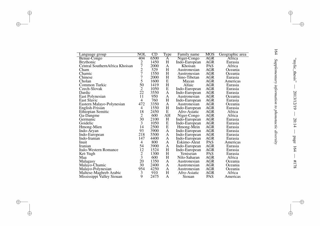
ii

“mylic_thesis”

—2013/12/19

—20:14

—page

164—

#178i

i

ii

ii

164Supplem

entaryinform

ationto

phonotacticdiversity

Language group NOL CD Type Family name MOS Geographic areaBenue-Congo 404 6500 A Niger-Congo AGR AfricaBrythonic 2 1450 H Indo-European AGR EurasiaCentral SouthernAfrica Khoisan 7 2000 A Khoisan PAS AfricaCham 2 529 H Austronesian AGR OceaniaChamic 7 1550 H Austronesian AGR OceaniaChinese 7 2000 H Sino-Tibetan AGR EurasiaCholan 5 1600 E Mayan AGR AmericasCommon Turkic 50 1419 H Altaic AGR EurasiaCzech-Slovak 2 1050 E Indo-European AGR EurasiaDardic 22 3550 A Indo-European AGR EurasiaEast Polynesian 11 950 A Austronesian AGR OceaniaEast Slavic 4 760 H Indo-European AGR EurasiaEastern Malayo-Polynesian 472 3350 A Austronesian AGR OceaniaEnglish-Frisian 4 1550 H Indo-European AGR EurasiaEthiopian Semitic 18 2450 E Afro-Asiatic AGR AfricaGa-Dangme 2 600 AH Niger-Congo AGR AfricaGermanic 30 2100 H Indo-European AGR EurasiaGoidelic 3 1050 E Indo-European AGR EurasiaHmong-Mien 14 2500 E Hmong-Mein AGR EurasiaIndo-Aryan 93 3900 A Indo-European AGR EurasiaIndo-European 218 5500 A Indo-European AGR EurasiaIndo-Iranian 147 4400 A Indo-European AGR EurasiaInuit 4 800 A Eskimo-Aleut PAS AmericasIranian 54 3900 A Indo-European AGR EurasiaItalo-Western Romance 12 1524 H Indo-European AGR EurasiaKet-Yugh 2 1300 H Yeniseian PAS EurasiaMaa 3 600 H Nilo-Saharan AGR AfricaMalagasy 20 1350 A Austronesian AGR OceaniaMalayo-Chamic 30 2400 A Austronesian AGR OceaniaMalayo-Polynesian 954 4250 A Austronesian AGR OceaniaMaltese-Maghreb Arabic 3 910 H Afro-Asiatic AGR AfricaMississippi Valley Siouan 9 2475 A Siouan PAS Americas

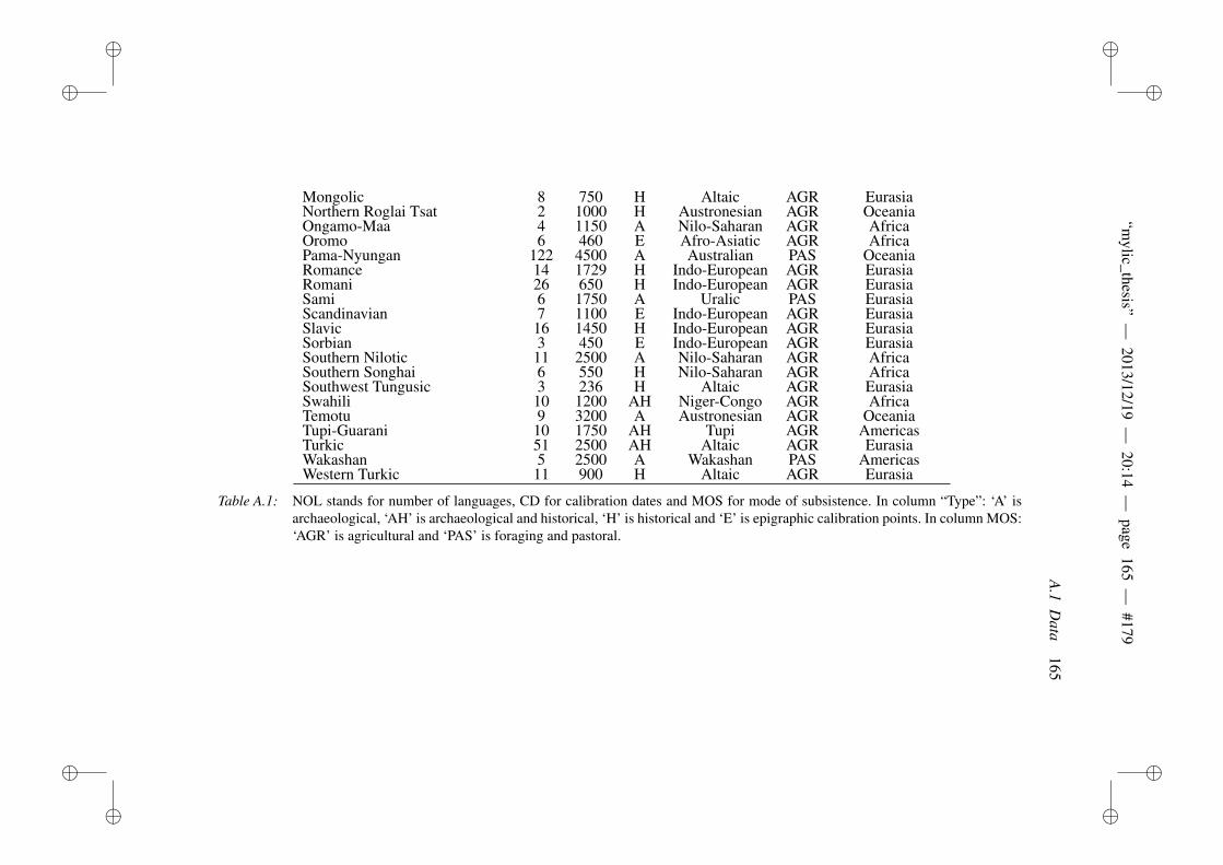
ii

“mylic_thesis”

—2013/12/19

—20:14

—page

165—

#179i

i

ii

ii

A.1

Data

165

Mongolic 8 750 H Altaic AGR EurasiaNorthern Roglai Tsat 2 1000 H Austronesian AGR OceaniaOngamo-Maa 4 1150 A Nilo-Saharan AGR AfricaOromo 6 460 E Afro-Asiatic AGR AfricaPama-Nyungan 122 4500 A Australian PAS OceaniaRomance 14 1729 H Indo-European AGR EurasiaRomani 26 650 H Indo-European AGR EurasiaSami 6 1750 A Uralic PAS EurasiaScandinavian 7 1100 E Indo-European AGR EurasiaSlavic 16 1450 H Indo-European AGR EurasiaSorbian 3 450 E Indo-European AGR EurasiaSouthern Nilotic 11 2500 A Nilo-Saharan AGR AfricaSouthern Songhai 6 550 H Nilo-Saharan AGR AfricaSouthwest Tungusic 3 236 H Altaic AGR EurasiaSwahili 10 1200 AH Niger-Congo AGR AfricaTemotu 9 3200 A Austronesian AGR OceaniaTupi-Guarani 10 1750 AH Tupi AGR AmericasTurkic 51 2500 AH Altaic AGR EurasiaWakashan 5 2500 A Wakashan PAS AmericasWestern Turkic 11 900 H Altaic AGR Eurasia

Table A.1: NOL stands for number of languages, CD for calibration dates and MOS for mode of subsistence. In column “Type”: ‘A’ isarchaeological, ‘AH’ is archaeological and historical, ‘H’ is historical and ‘E’ is epigraphic calibration points. In column MOS:‘AGR’ is agricultural and ‘PAS’ is foraging and pastoral.

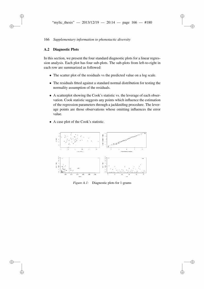
ii


ii

ii

166 Supplementary information to phonotactic diversity

A.2 Diagnostic Plots

In this section, we present the four standard diagnostic plots for a linear regres-sion analysis. Each plot has four sub-plots. The sub-plots from left-to-right ineach row are summarized as followed:

• The scatter plot of the residuals vs the predicted value on a log scale.

• The residuals fitted against a standard normal distribution for testing thenormality assumption of the residuals.

• A scatterplot showing the Cook’s statistic vs. the leverage of each obser-vation. Cook statistic suggests any points which influence the estimationof the regression parameters through a jackknifing procedure. The lever-age points are those observations whose omitting influences the errorvalue.

• A case plot of the Cook’s statistic.

Figure A.1: Diagnostic plots for 1-grams

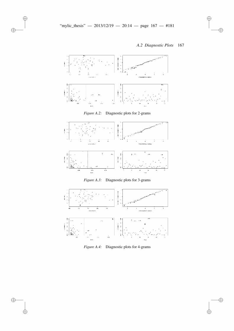
ii


ii

ii

A.2 Diagnostic Plots 167




ii


ii

ii



ii


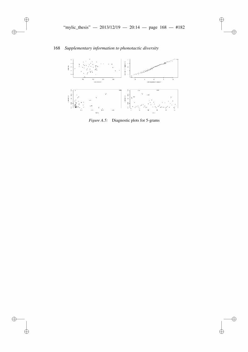
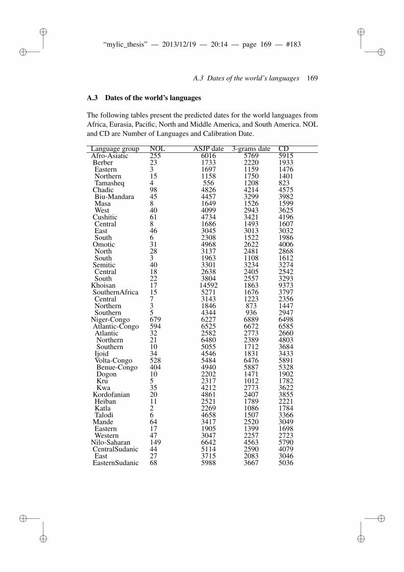
ii

ii

A.3 Dates of the world’s languages 169

A.3 Dates of the world’s languages

The following tables present the predicted dates for the world languages fromAfrica, Eurasia, Pacific, North and Middle America, and South America. NOLand CD are Number of Languages and Calibration Date.

Language group NOL ASJP date 3-grams date CDAfro-Asiatic 255 6016 5769 5915Berber 23 1733 2220 1933Eastern 3 1697 1159 1476Northern 15 1158 1750 1401Tamasheq 4 556 1208 823

Chadic 98 4826 4214 4575Biu-Mandara 45 4457 3299 3982Masa 8 1649 1526 1599West 40 4099 2943 3625

Cushitic 61 4734 3421 4196Central 8 1686 1493 1607East 46 3045 3013 3032South 6 2308 1522 1986

Omotic 31 4968 2622 4006North 28 3137 2481 2868South 3 1963 1108 1612

Semitic 40 3301 3234 3274Central 18 2638 2405 2542South 22 3804 2557 3293

Khoisan 17 14592 1863 9373SouthernAfrica 15 5271 1676 3797Central 7 3143 1223 2356Northern 3 1846 873 1447Southern 5 4344 936 2947

Niger-Congo 679 6227 6889 6498Atlantic-Congo 594 6525 6672 6585Atlantic 32 2582 2773 2660Northern 21 6480 2389 4803Southern 10 5055 1712 3684Ijoid 34 4546 1831 3433Volta-Congo 528 5484 6476 5891Benue-Congo 404 4940 5887 5328Dogon 10 2202 1471 1902Kru 5 2317 1012 1782Kwa 35 4212 2773 3622

Kordofanian 20 4861 2407 3855Heiban 11 2521 1789 2221Katla 2 2269 1086 1784Talodi 6 4658 1507 3366

Mande 64 3417 2520 3049Eastern 17 1905 1399 1698Western 47 3047 2257 2723

Nilo-Saharan 149 6642 4563 5790CentralSudanic 44 5114 2590 4079East 27 3715 2083 3046

EasternSudanic 68 5988 3667 5036

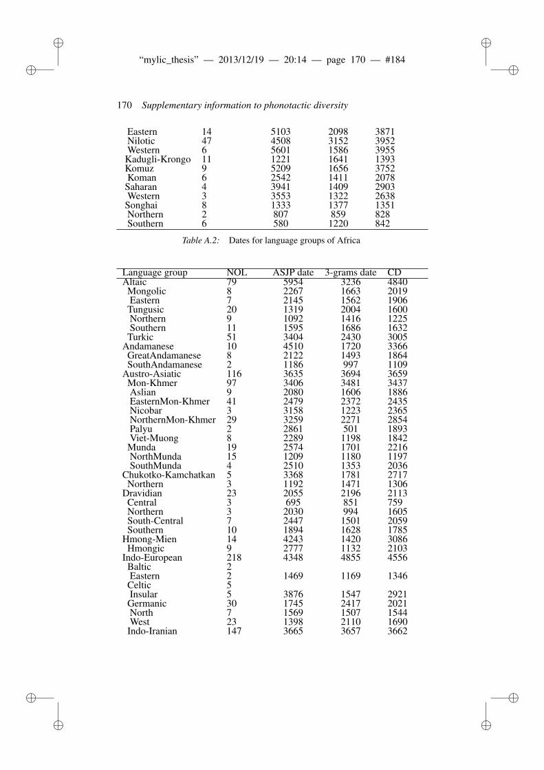
ii


ii

ii


Eastern 14 5103 2098 3871Nilotic 47 4508 3152 3952Western 6 5601 1586 3955

Kadugli-Krongo 11 1221 1641 1393Komuz 9 5209 1656 3752Koman 6 2542 1411 2078

Saharan 4 3941 1409 2903Western 3 3553 1322 2638

Songhai 8 1333 1377 1351Northern 2 807 859 828Southern 6 580 1220 842

Table A.2: Dates for language groups of Africa

Language group NOL ASJP date 3-grams date CDAltaic 79 5954 3236 4840

Mongolic 8 2267 1663 2019Eastern 7 2145 1562 1906Tungusic 20 1319 2004 1600Northern 9 1092 1416 1225Southern 11 1595 1686 1632Turkic 51 3404 2430 3005

Andamanese 10 4510 1720 3366GreatAndamanese 8 2122 1493 1864SouthAndamanese 2 1186 997 1109

Austro-Asiatic 116 3635 3694 3659Mon-Khmer 97 3406 3481 3437Aslian 9 2080 1606 1886EasternMon-Khmer 41 2479 2372 2435Nicobar 3 3158 1223 2365NorthernMon-Khmer 29 3259 2271 2854Palyu 2 2861 501 1893Viet-Muong 8 2289 1198 1842Munda 19 2574 1701 2216NorthMunda 15 1209 1180 1197SouthMunda 4 2510 1353 2036

Chukotko-Kamchatkan 5 3368 1781 2717Northern 3 1192 1471 1306

Dravidian 23 2055 2196 2113Central 3 695 851 759Northern 3 2030 994 1605South-Central 7 2447 1501 2059Southern 10 1894 1628 1785

Hmong-Mien 14 4243 1420 3086Hmongic 9 2777 1132 2103

Indo-European 218 4348 4855 4556Baltic 2Eastern 2 1469 1169 1346Celtic 5Insular 5 3876 1547 2921Germanic 30 1745 2417 2021North 7 1569 1507 1544West 23 1398 2110 1690Indo-Iranian 147 3665 3657 3662

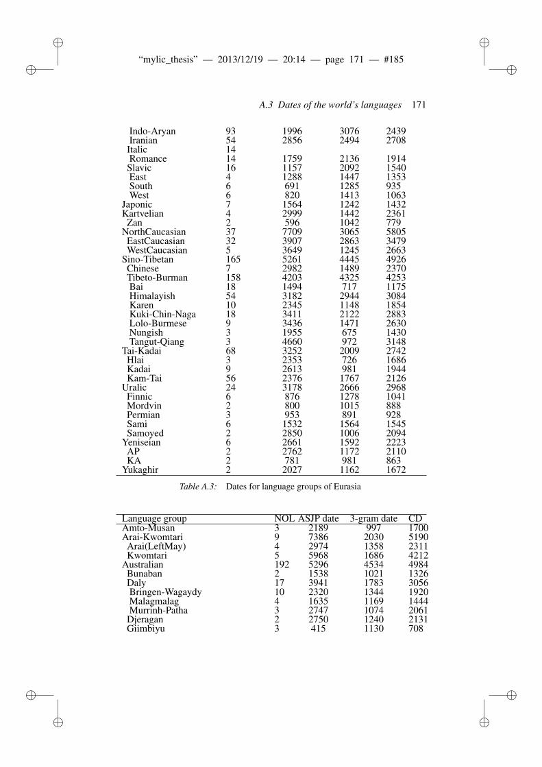
ii


ii

ii


Indo-Aryan 93 1996 3076 2439Iranian 54 2856 2494 2708Italic 14Romance 14 1759 2136 1914Slavic 16 1157 2092 1540East 4 1288 1447 1353South 6 691 1285 935West 6 820 1413 1063

Japonic 7 1564 1242 1432Kartvelian 4 2999 1442 2361

Zan 2 596 1042 779NorthCaucasian 37 7709 3065 5805

EastCaucasian 32 3907 2863 3479WestCaucasian 5 3649 1245 2663

Sino-Tibetan 165 5261 4445 4926Chinese 7 2982 1489 2370Tibeto-Burman 158 4203 4325 4253Bai 18 1494 717 1175Himalayish 54 3182 2944 3084Karen 10 2345 1148 1854Kuki-Chin-Naga 18 3411 2122 2883Lolo-Burmese 9 3436 1471 2630Nungish 3 1955 675 1430Tangut-Qiang 3 4660 972 3148

Tai-Kadai 68 3252 2009 2742Hlai 3 2353 726 1686Kadai 9 2613 981 1944Kam-Tai 56 2376 1767 2126

Uralic 24 3178 2666 2968Finnic 6 876 1278 1041Mordvin 2 800 1015 888Permian 3 953 891 928Sami 6 1532 1564 1545Samoyed 2 2850 1006 2094

Yeniseian 6 2661 1592 2223AP 2 2762 1172 2110KA 2 781 981 863

Yukaghir 2 2027 1162 1672

Table A.3: Dates for language groups of Eurasia

Language group NOL ASJP date 3-gram date CDAmto-Musan 3 2189 997 1700Arai-Kwomtari 9 7386 2030 5190

Arai(LeftMay) 4 2974 1358 2311Kwomtari 5 5968 1686 4212

Australian 192 5296 4534 4984Bunaban 2 1538 1021 1326Daly 17 3941 1783 3056Bringen-Wagaydy 10 2320 1344 1920Malagmalag 4 1635 1169 1444Murrinh-Patha 3 2747 1074 2061Djeragan 2 2750 1240 2131Giimbiyu 3 415 1130 708

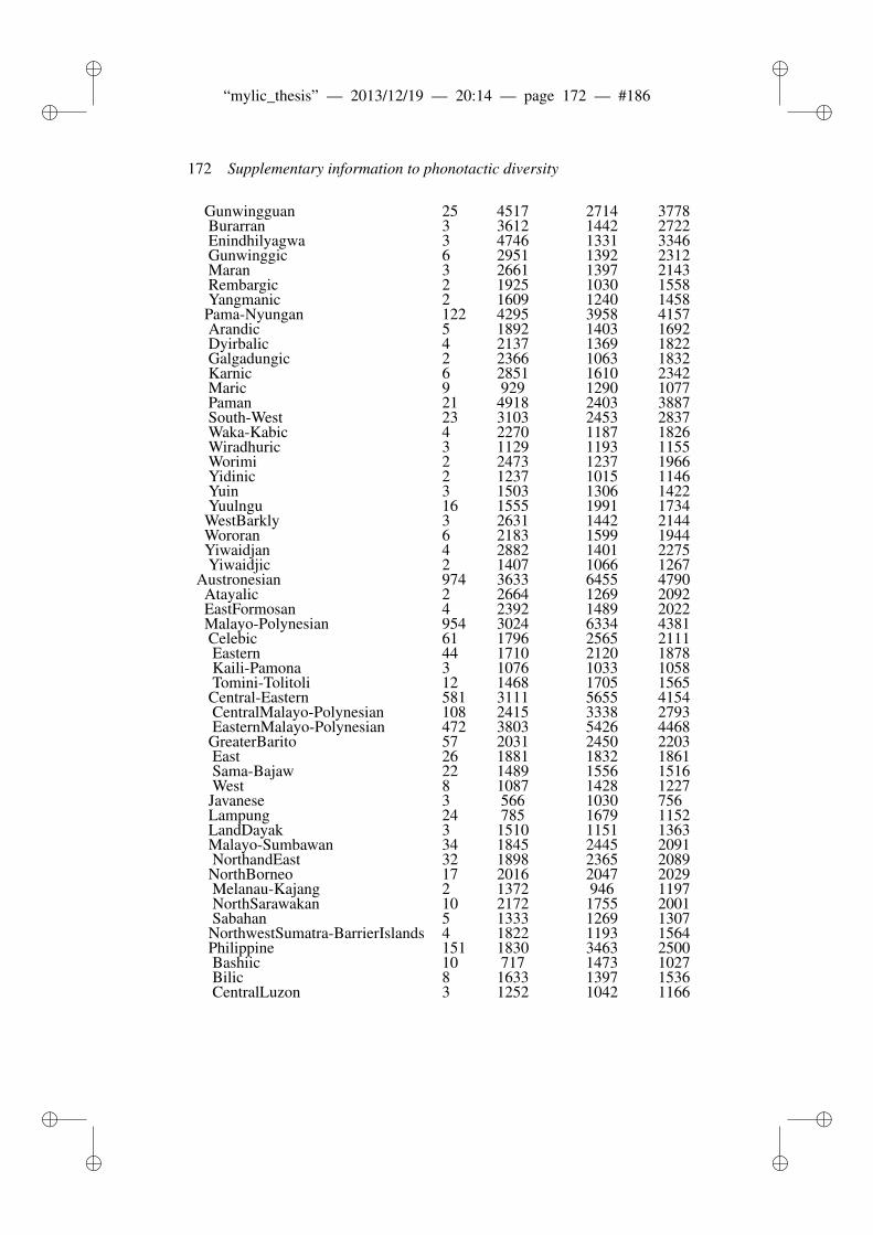
ii


ii

ii


Gunwingguan 25 4517 2714 3778Burarran 3 3612 1442 2722Enindhilyagwa 3 4746 1331 3346Gunwinggic 6 2951 1392 2312Maran 3 2661 1397 2143Rembargic 2 1925 1030 1558Yangmanic 2 1609 1240 1458Pama-Nyungan 122 4295 3958 4157Arandic 5 1892 1403 1692Dyirbalic 4 2137 1369 1822Galgadungic 2 2366 1063 1832Karnic 6 2851 1610 2342Maric 9 929 1290 1077Paman 21 4918 2403 3887South-West 23 3103 2453 2837Waka-Kabic 4 2270 1187 1826Wiradhuric 3 1129 1193 1155Worimi 2 2473 1237 1966Yidinic 2 1237 1015 1146Yuin 3 1503 1306 1422Yuulngu 16 1555 1991 1734WestBarkly 3 2631 1442 2144Wororan 6 2183 1599 1944Yiwaidjan 4 2882 1401 2275Yiwaidjic 2 1407 1066 1267

Austronesian 974 3633 6455 4790Atayalic 2 2664 1269 2092EastFormosan 4 2392 1489 2022Malayo-Polynesian 954 3024 6334 4381Celebic 61 1796 2565 2111Eastern 44 1710 2120 1878Kaili-Pamona 3 1076 1033 1058Tomini-Tolitoli 12 1468 1705 1565Central-Eastern 581 3111 5655 4154CentralMalayo-Polynesian 108 2415 3338 2793EasternMalayo-Polynesian 472 3803 5426 4468GreaterBarito 57 2031 2450 2203East 26 1881 1832 1861Sama-Bajaw 22 1489 1556 1516West 8 1087 1428 1227Javanese 3 566 1030 756Lampung 24 785 1679 1152LandDayak 3 1510 1151 1363Malayo-Sumbawan 34 1845 2445 2091NorthandEast 32 1898 2365 2089NorthBorneo 17 2016 2047 2029Melanau-Kajang 2 1372 946 1197NorthSarawakan 10 2172 1755 2001Sabahan 5 1333 1269 1307NorthwestSumatra-BarrierIslands 4 1822 1193 1564Philippine 151 1830 3463 2500Bashiic 10 717 1473 1027Bilic 8 1633 1397 1536CentralLuzon 3 1252 1042 1166

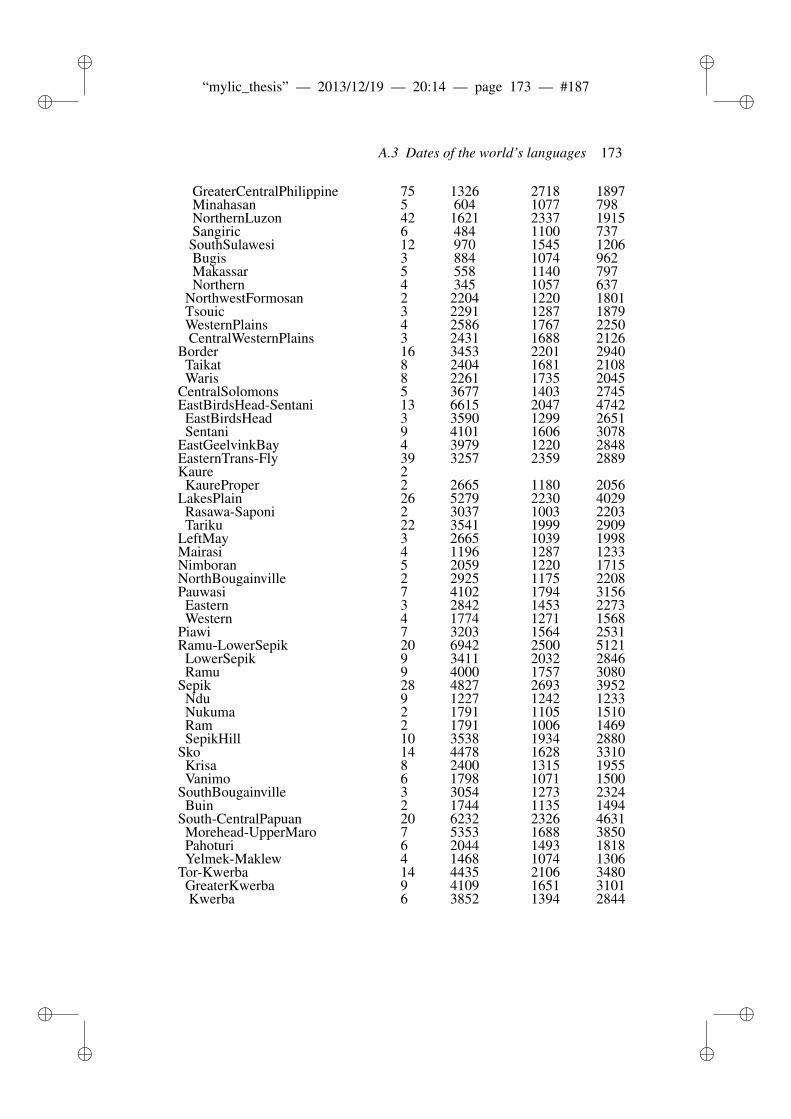
ii


ii

ii


GreaterCentralPhilippine 75 1326 2718 1897Minahasan 5 604 1077 798NorthernLuzon 42 1621 2337 1915Sangiric 6 484 1100 737SouthSulawesi 12 970 1545 1206Bugis 3 884 1074 962Makassar 5 558 1140 797Northern 4 345 1057 637

NorthwestFormosan 2 2204 1220 1801Tsouic 3 2291 1287 1879WesternPlains 4 2586 1767 2250CentralWesternPlains 3 2431 1688 2126

Border 16 3453 2201 2940Taikat 8 2404 1681 2108Waris 8 2261 1735 2045

CentralSolomons 5 3677 1403 2745EastBirdsHead-Sentani 13 6615 2047 4742

EastBirdsHead 3 3590 1299 2651Sentani 9 4101 1606 3078

EastGeelvinkBay 4 3979 1220 2848EasternTrans-Fly 39 3257 2359 2889Kaure 2

KaureProper 2 2665 1180 2056LakesPlain 26 5279 2230 4029

Rasawa-Saponi 2 3037 1003 2203Tariku 22 3541 1999 2909

LeftMay 3 2665 1039 1998Mairasi 4 1196 1287 1233Nimboran 5 2059 1220 1715NorthBougainville 2 2925 1175 2208Pauwasi 7 4102 1794 3156

Eastern 3 2842 1453 2273Western 4 1774 1271 1568

Piawi 7 3203 1564 2531Ramu-LowerSepik 20 6942 2500 5121

LowerSepik 9 3411 2032 2846Ramu 9 4000 1757 3080

Sepik 28 4827 2693 3952Ndu 9 1227 1242 1233Nukuma 2 1791 1105 1510Ram 2 1791 1006 1469SepikHill 10 3538 1934 2880

Sko 14 4478 1628 3310Krisa 8 2400 1315 1955Vanimo 6 1798 1071 1500

SouthBougainville 3 3054 1273 2324Buin 2 1744 1135 1494

South-CentralPapuan 20 6232 2326 4631Morehead-UpperMaro 7 5353 1688 3850Pahoturi 6 2044 1493 1818Yelmek-Maklew 4 1468 1074 1306

Tor-Kwerba 14 4435 2106 3480GreaterKwerba 9 4109 1651 3101Kwerba 6 3852 1394 2844

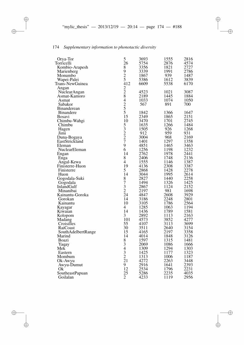
ii


ii

ii


Orya-Tor 5 3693 1555 2816Torricelli 26 5754 2876 4574

Kombio-Arapesh 8 3356 1821 2727Marienberg 9 3339 1991 2786Monumbo 2 1867 939 1487Wapei-Palei 5 5386 1612 3839

Trans-NewGuinea 412 6609 5538 6170Angan 2NuclearAngan 2 4523 1021 3087Asmat-Kamoro 8 2189 1445 1884Asmat 4 1033 1074 1050Sabakor 2 567 891 700Binanderean 5Binandere 5 1842 1366 1647Bosavi 15 2349 1865 2151Chimbu-Wahgi 10 3470 1701 2745Chimbu 5 1635 1266 1484Hagen 3 1505 926 1268Jimi 2 912 959 931Duna-Bogaya 2 3004 968 2169EastStrickland 7 1401 1297 1358Eleman 9 4851 1465 3463NuclearEleman 6 1256 1198 1232Engan 14 2762 1978 2441Enga 8 2406 1748 2136Angal-Kewa 4 1555 1146 1387Finisterre-Huon 19 4136 2308 3387Finisterre 5 2868 1428 2278Huon 14 3044 1995 2614Gogodala-Suki 8 2827 1440 2258Gogodala 7 1494 1326 1425InlandGulf 3 2867 1124 2152Minanibai 2 2197 981 1698Kainantu-Goroka 24 4847 2608 3929Gorokan 14 3186 2248 2801Kainantu 10 3105 1786 2564Kayagar 4 1285 1063 1194Kiwaian 14 1436 1789 1581Kolopom 3 2892 1113 2163Madang 101 4573 3852 4277Croisilles 55 4107 3113 3699RaiCoast 30 3511 2640 3154SouthAdelbertRange 15 4165 2197 3358Marind 14 4014 1848 3126Boazi 8 1597 1315 1481Yaqay 3 2069 1086 1666Mek 4 1309 1294 1303Eastern 3 1425 1177 1323Mombum 2 1313 1006 1187Ok-Awyu 21 4272 2263 3448Awyu-Dumut 9 2916 1641 2393Ok 12 2534 1796 2231SoutheastPapuan 25 5286 2235 4035Goilalan 2 4233 1119 2956

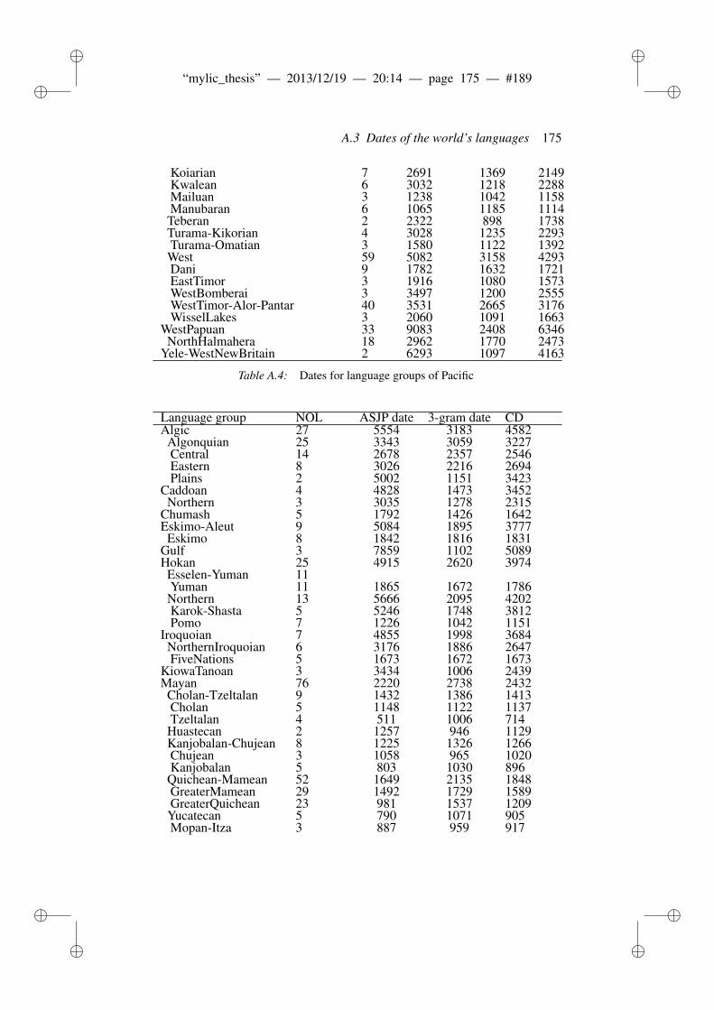
ii


ii

ii


Koiarian 7 2691 1369 2149Kwalean 6 3032 1218 2288Mailuan 3 1238 1042 1158Manubaran 6 1065 1185 1114Teberan 2 2322 898 1738Turama-Kikorian 4 3028 1235 2293Turama-Omatian 3 1580 1122 1392West 59 5082 3158 4293Dani 9 1782 1632 1721EastTimor 3 1916 1080 1573WestBomberai 3 3497 1200 2555WestTimor-Alor-Pantar 40 3531 2665 3176WisselLakes 3 2060 1091 1663

WestPapuan 33 9083 2408 6346NorthHalmahera 18 2962 1770 2473

Yele-WestNewBritain 2 6293 1097 4163

Table A.4: Dates for language groups of Pacific

Language group NOL ASJP date 3-gram date CDAlgic 27 5554 3183 4582

Algonquian 25 3343 3059 3227Central 14 2678 2357 2546Eastern 8 3026 2216 2694Plains 2 5002 1151 3423

Caddoan 4 4828 1473 3452Northern 3 3035 1278 2315

Chumash 5 1792 1426 1642Eskimo-Aleut 9 5084 1895 3777

Eskimo 8 1842 1816 1831Gulf 3 7859 1102 5089Hokan 25 4915 2620 3974

Esselen-Yuman 11Yuman 11 1865 1672 1786Northern 13 5666 2095 4202Karok-Shasta 5 5246 1748 3812Pomo 7 1226 1042 1151

Iroquoian 7 4855 1998 3684NorthernIroquoian 6 3176 1886 2647FiveNations 5 1673 1672 1673

KiowaTanoan 3 3434 1006 2439Mayan 76 2220 2738 2432

Cholan-Tzeltalan 9 1432 1386 1413Cholan 5 1148 1122 1137Tzeltalan 4 511 1006 714Huastecan 2 1257 946 1129Kanjobalan-Chujean 8 1225 1326 1266Chujean 3 1058 965 1020Kanjobalan 5 803 1030 896Quichean-Mamean 52 1649 2135 1848GreaterMamean 29 1492 1729 1589GreaterQuichean 23 981 1537 1209Yucatecan 5 790 1071 905Mopan-Itza 3 887 959 917

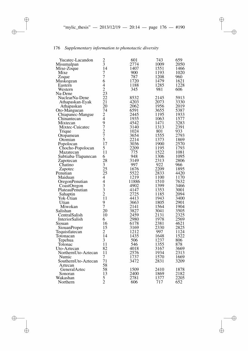
ii


ii

ii


Yucatec-Lacandon 2 601 743 659Misumalpan 3 2774 1009 2050Mixe-Zoque 14 1407 1551 1466

Mixe 7 900 1193 1020Zoque 7 787 1208 960

Muskogean 6 1720 1479 1621Eastern 4 1188 1285 1228Western 2 345 981 606

Na-Dene 23NuclearNa-Dene 22 8532 2145 5913Athapaskan-Eyak 21 4203 2073 3330Athapaskan 20 2062 1956 2019

Oto-Manguean 74 6591 3655 5387Chiapanec-Mangue 2 2445 1195 1933Chinantecan 4 1935 1063 1577Mixtecan 9 4542 1471 3283Mixtec-Cuicatec 7 3140 1313 2391Trique 2 1024 801 933Otopamean 7 3654 1555 2793Otomian 5 2214 1373 1869Popolocan 17 3036 1900 2570Chocho-Popolocan 5 2209 1195 1793Mazatecan 11 775 1522 1081Subtiaba-Tlapanecan 6 948 1306 1095Zapotecan 28 3149 2313 2806Chatino 3 997 922 966Zapotec 25 1676 2209 1895

Penutian 25 5522 2833 4420Maiduan 4 1219 1100 1170OregonPenutian 4 11886 1510 7632CoastOregon 3 4902 1399 3466PlateauPenutian 3 4147 1353 3001Sahaptin 2 2725 1185 2094Yok-Utian 11 4413 1943 3400Utian 9 3663 1805 2901Miwokan 7 2141 1564 1904

Salishan 20 3827 3041 3505CentralSalish 10 2459 2131 2325InteriorSalish 6 2980 1978 2569

Siouan 16 6178 2381 4621SiouanProper 15 3169 2330 2825

Tequistlatecan 2 1212 997 1124Totonacan 14 1435 1648 1522

Tepehua 3 506 1237 806Totonac 11 546 1355 878

Uto-Aztecan 82 4018 3167 3669NorthernUto-Aztecan 11 2576 1934 2313Numic 7 1737 1570 1669SouthernUto-Aztecan 71 3472 2831 3209Aztecan 58GeneralAztec 58 1509 2410 1878Sonoran 13 2400 1869 2182

Wakashan 5 2781 1377 2205Northern 2 606 717 652

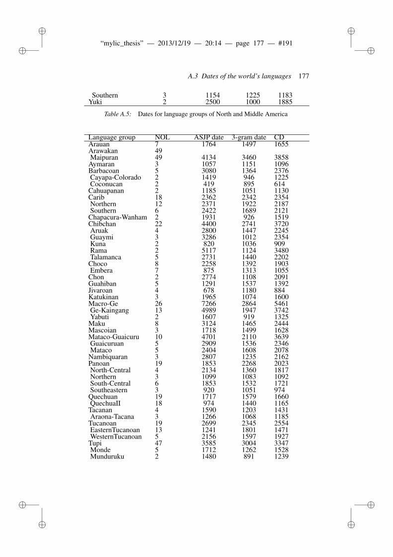
ii


ii

ii


Southern 3 1154 1225 1183Yuki 2 2500 1000 1885

Table A.5: Dates for language groups of North and Middle America

Language group NOL ASJP date 3-gram date CDArauan 7 1764 1497 1655Arawakan 49Maipuran 49 4134 3460 3858Aymaran 3 1057 1151 1096Barbacoan 5 3080 1364 2376Cayapa-Colorado 2 1419 946 1225Coconucan 2 419 895 614Cahuapanan 2 1185 1051 1130Carib 18 2362 2342 2354Northern 12 2371 1922 2187Southern 6 2422 1689 2121Chapacura-Wanham 2 1931 926 1519Chibchan 22 4400 2741 3720Aruak 4 2800 1447 2245Guaymi 3 3286 1012 2354Kuna 2 820 1036 909Rama 2 5117 1124 3480Talamanca 5 2731 1440 2202Choco 8 2258 1392 1903Embera 7 875 1313 1055Chon 2 2774 1108 2091Guahiban 5 1291 1537 1392Jivaroan 4 678 1180 884Katukinan 3 1965 1074 1600Macro-Ge 26 7266 2864 5461Ge-Kaingang 13 4989 1947 3742Yabuti 2 1607 919 1325Maku 8 3124 1465 2444Mascoian 3 1718 1499 1628Mataco-Guaicuru 10 4701 2110 3639Guaicuruan 5 2909 1536 2346Mataco 5 2404 1608 2078Nambiquaran 3 2807 1235 2162Panoan 19 1853 2268 2023North-Central 4 2134 1360 1817Northern 3 1099 1083 1092South-Central 6 1853 1532 1721Southeastern 3 920 1051 974Quechuan 19 1717 1579 1660QuechuaII 18 974 1440 1165Tacanan 4 1590 1203 1431Araona-Tacana 3 1266 1068 1185Tucanoan 19 2699 2345 2554EasternTucanoan 13 1241 1801 1471WesternTucanoan 5 2156 1597 1927Tupi 47 3585 3004 3347Monde 5 1712 1262 1528Munduruku 2 1480 891 1239

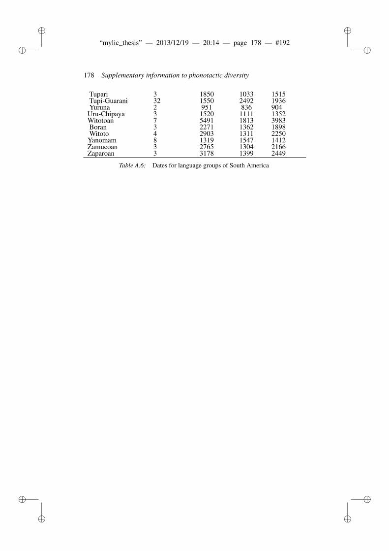
ii


ii

ii


Tupari 3 1850 1033 1515Tupi-Guarani 32 1550 2492 1936Yuruna 2 951 836 904Uru-Chipaya 3 1520 1111 1352Witotoan 7 5491 1813 3983Boran 3 2271 1362 1898Witoto 4 2903 1311 2250Yanomam 8 1319 1547 1412Zamucoan 3 2765 1304 2166Zaparoan 3 3178 1399 2449

Table A.6: Dates for language groups of South America

ii


ii

ii

B APPENDIX TO EVALUATION

OF STRING SIMILARITY

MEASURES

This chapter contains the supplementary information to the tables referred inpaper V.

B.1 Results for string similarity

The tables B.1, B.2, and B.3 show the family averages of Goodman-Kruskal’sGamma, distinctiveness score, and WALS r for different string similarity mea-sures.

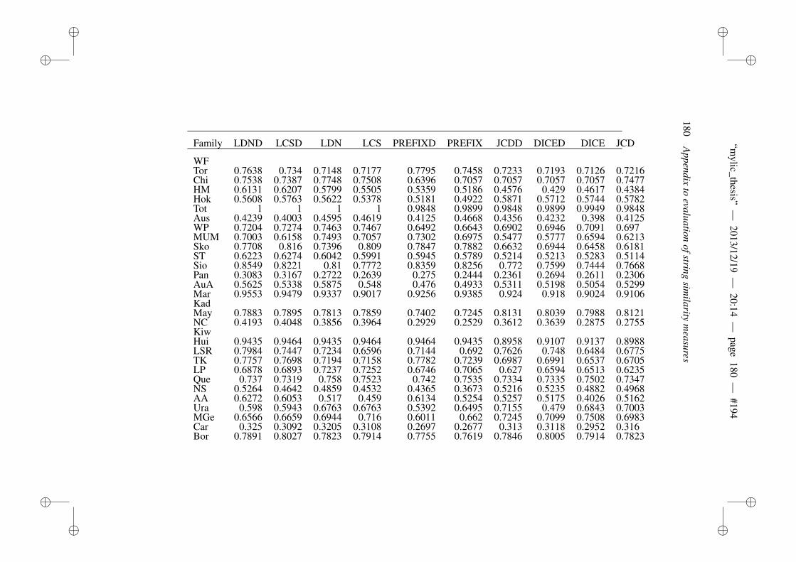
ii

“mylic_thesis”

—2013/12/19

—20:14

—page

180—

#194i

i

ii

ii

180A

ppendixto

evaluationofstring

similarity

measures

Family LDND LCSD LDN LCS PREFIXD PREFIX JCDD DICED DICE JCD

WFTor 0.7638 0.734 0.7148 0.7177 0.7795 0.7458 0.7233 0.7193 0.7126 0.7216Chi 0.7538 0.7387 0.7748 0.7508 0.6396 0.7057 0.7057 0.7057 0.7057 0.7477HM 0.6131 0.6207 0.5799 0.5505 0.5359 0.5186 0.4576 0.429 0.4617 0.4384Hok 0.5608 0.5763 0.5622 0.5378 0.5181 0.4922 0.5871 0.5712 0.5744 0.5782Tot 1 1 1 1 0.9848 0.9899 0.9848 0.9899 0.9949 0.9848Aus 0.4239 0.4003 0.4595 0.4619 0.4125 0.4668 0.4356 0.4232 0.398 0.4125WP 0.7204 0.7274 0.7463 0.7467 0.6492 0.6643 0.6902 0.6946 0.7091 0.697MUM 0.7003 0.6158 0.7493 0.7057 0.7302 0.6975 0.5477 0.5777 0.6594 0.6213Sko 0.7708 0.816 0.7396 0.809 0.7847 0.7882 0.6632 0.6944 0.6458 0.6181ST 0.6223 0.6274 0.6042 0.5991 0.5945 0.5789 0.5214 0.5213 0.5283 0.5114Sio 0.8549 0.8221 0.81 0.7772 0.8359 0.8256 0.772 0.7599 0.7444 0.7668Pan 0.3083 0.3167 0.2722 0.2639 0.275 0.2444 0.2361 0.2694 0.2611 0.2306AuA 0.5625 0.5338 0.5875 0.548 0.476 0.4933 0.5311 0.5198 0.5054 0.5299Mar 0.9553 0.9479 0.9337 0.9017 0.9256 0.9385 0.924 0.918 0.9024 0.9106KadMay 0.7883 0.7895 0.7813 0.7859 0.7402 0.7245 0.8131 0.8039 0.7988 0.8121NC 0.4193 0.4048 0.3856 0.3964 0.2929 0.2529 0.3612 0.3639 0.2875 0.2755KiwHui 0.9435 0.9464 0.9435 0.9464 0.9464 0.9435 0.8958 0.9107 0.9137 0.8988LSR 0.7984 0.7447 0.7234 0.6596 0.7144 0.692 0.7626 0.748 0.6484 0.6775TK 0.7757 0.7698 0.7194 0.7158 0.7782 0.7239 0.6987 0.6991 0.6537 0.6705LP 0.6878 0.6893 0.7237 0.7252 0.6746 0.7065 0.627 0.6594 0.6513 0.6235Que 0.737 0.7319 0.758 0.7523 0.742 0.7535 0.7334 0.7335 0.7502 0.7347NS 0.5264 0.4642 0.4859 0.4532 0.4365 0.3673 0.5216 0.5235 0.4882 0.4968AA 0.6272 0.6053 0.517 0.459 0.6134 0.5254 0.5257 0.5175 0.4026 0.5162Ura 0.598 0.5943 0.6763 0.6763 0.5392 0.6495 0.7155 0.479 0.6843 0.7003MGe 0.6566 0.6659 0.6944 0.716 0.6011 0.662 0.7245 0.7099 0.7508 0.6983Car 0.325 0.3092 0.3205 0.3108 0.2697 0.2677 0.313 0.3118 0.2952 0.316Bor 0.7891 0.8027 0.7823 0.7914 0.7755 0.7619 0.7846 0.8005 0.7914 0.7823

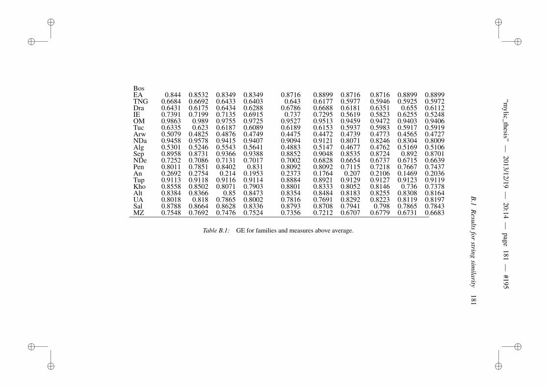
ii

“mylic_thesis”

—2013/12/19

—20:14

—page

181—

#195i

i

ii

ii

B.1

Results

forstring

similarity

181

BosEA 0.844 0.8532 0.8349 0.8349 0.8716 0.8899 0.8716 0.8716 0.8899 0.8899TNG 0.6684 0.6692 0.6433 0.6403 0.643 0.6177 0.5977 0.5946 0.5925 0.5972Dra 0.6431 0.6175 0.6434 0.6288 0.6786 0.6688 0.6181 0.6351 0.655 0.6112IE 0.7391 0.7199 0.7135 0.6915 0.737 0.7295 0.5619 0.5823 0.6255 0.5248OM 0.9863 0.989 0.9755 0.9725 0.9527 0.9513 0.9459 0.9472 0.9403 0.9406Tuc 0.6335 0.623 0.6187 0.6089 0.6189 0.6153 0.5937 0.5983 0.5917 0.5919Arw 0.5079 0.4825 0.4876 0.4749 0.4475 0.4472 0.4739 0.4773 0.4565 0.4727NDa 0.9458 0.9578 0.9415 0.9407 0.9094 0.9121 0.8071 0.8246 0.8304 0.8009Alg 0.5301 0.5246 0.5543 0.5641 0.4883 0.5147 0.4677 0.4762 0.5169 0.5106Sep 0.8958 0.8731 0.9366 0.9388 0.8852 0.9048 0.8535 0.8724 0.892 0.8701NDe 0.7252 0.7086 0.7131 0.7017 0.7002 0.6828 0.6654 0.6737 0.6715 0.6639Pen 0.8011 0.7851 0.8402 0.831 0.8092 0.8092 0.7115 0.7218 0.7667 0.7437An 0.2692 0.2754 0.214 0.1953 0.2373 0.1764 0.207 0.2106 0.1469 0.2036Tup 0.9113 0.9118 0.9116 0.9114 0.8884 0.8921 0.9129 0.9127 0.9123 0.9119Kho 0.8558 0.8502 0.8071 0.7903 0.8801 0.8333 0.8052 0.8146 0.736 0.7378Alt 0.8384 0.8366 0.85 0.8473 0.8354 0.8484 0.8183 0.8255 0.8308 0.8164UA 0.8018 0.818 0.7865 0.8002 0.7816 0.7691 0.8292 0.8223 0.8119 0.8197Sal 0.8788 0.8664 0.8628 0.8336 0.8793 0.8708 0.7941 0.798 0.7865 0.7843MZ 0.7548 0.7692 0.7476 0.7524 0.7356 0.7212 0.6707 0.6779 0.6731 0.6683

Table B.1: GE for families and measures above average.

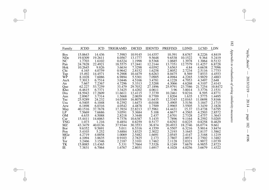
ii

“mylic_thesis”

—2013/12/19

—20:14

—page

182—

#196i

i

ii

ii

182A

ppendixto

evaluationofstring

similarity

measures

Family JCDD JCD TRIGRAMD DICED IDENTD PREFIXD LDND LCSD LDN

Bos 15.0643 14.436 7.5983 10.9145 14.4357 10.391 8.6767 8.2226 4.8419NDe 19.8309 19.2611 8.0567 13.1777 9.5648 9.6538 10.1522 9.364 5.2419NC 1.7703 1.6102 0.6324 1.1998 0.5368 1.0685 1.3978 1.3064 0.5132Pan 24.7828 22.4921 18.5575 17.2441 12.2144 13.7351 12.7579 11.4257 6.8728Hok 10.2645 9.826 3.6634 7.3298 4.0392 3.6563 4.84 4.6638 2.7096Chi 4.165 4.0759 0.9642 2.8152 1.6258 2.8052 2.7234 2.5116 1.7753Tup 15.492 14.4571 9.2908 10.4479 6.6263 8.0475 8.569 7.8533 4.4553WP 8.1028 7.6086 6.9894 5.5301 7.0905 4.0984 4.2265 3.9029 2.4883AuA 7.3013 6.7514 3.0446 4.5166 3.4781 4.1228 4.7953 4.3497 2.648An 7.667 7.2367 4.7296 5.3313 2.5288 4.3066 4.6268 4.3107 2.4143Que 62.227 53.7259 33.479 29.7032 27.1896 25.9791 23.7586 21.7254 10.8472Kho 6.4615 6.7371 3.3425 4.4202 4.0611 3.96 3.8014 3.3776 2.1531Dra 18.5943 17.2609 11.6611 12.4115 7.3739 10.2461 9.8216 8.595 4.8771Aus 2.8967 3.7314 1.5668 2.0659 0.7709 1.8204 1.635 1.5775 1.4495Tuc 25.9289 24.232 14.0369 16.8078 11.6435 12.5345 12.0163 11.0698 5.8166Ura 6.5405 6.1048 0.2392 1.6473 -0.0108 3.4905 3.5156 3.1847 2.1715Arw 6.1898 6.0316 4.0542 4.4878 1.7509 2.9965 3.5505 3.3439 2.1828May 40.1516 37.7678 17.3924 22.8213 17.5961 14.4431 15.37 13.4738 7.6795LP 7.5669 7.6686 3.0591 5.3684 5.108 4.8677 4.3565 4.2503 2.8572OM 4.635 4.5088 2.8218 3.3448 2.437 2.6701 2.7328 2.4757 1.3643Car 15.4411 14.6063 9.7376 10.6387 5.1435 7.7896 9.1164 8.2592 5.0205TNG 1.073 1.216 0.4854 0.8259 0.5177 0.8292 0.8225 0.8258 0.4629MZ 43.3479 40.0136 37.9344 30.3553 36.874 20.4933 18.2746 16.0774 9.661Bor 9.6352 9.5691 5.011 6.5316 4.1559 6.5507 6.3216 5.9014 3.8474Pen 5.4103 5.252 3.6884 3.8325 2.3022 3.2193 3.1645 2.8137 1.5862MGe 4.2719 4.0058 1.0069 2.5482 1.6691 2.0545 2.4147 2.3168 1.1219ST 4.1094 3.8635 0.9103 2.7825 2.173 2.7807 2.8974 2.7502 1.3482Tor 3.2466 3.1546 2.2187 2.3101 1.7462 2.1128 2.0321 1.9072 1.0739TK 15.0085 13.4365 5.331 7.7664 7.5326 8.1249 7.6679 6.9855 2.8723IE 7.3831 6.7064 1.6767 2.8031 1.6917 4.1028 4.0256 3.6679 1.4322

ii

“mylic_thesis”

—2013/12/19

—20:14

—page

183—

#197i

i

ii

ii

B.1

Results

forstring

similarity

183

Alg 6.8582 6.737 4.5117 5.2475 1.2071 4.5916 5.2534 4.5017 2.775NS 2.4402 2.3163 1.1485 1.6505 1.1456 1.321 1.3681 1.3392 0.6085Sko 6.7676 6.3721 2.5992 4.6468 4.7931 5.182 4.7014 4.5975 2.5371AA 1.8054 1.6807 0.7924 1.2557 0.4923 1.37 1.3757 1.3883 0.6411LSR 4.0791 4.3844 2.2048 2.641 1.5778 2.1808 2.1713 2.0826 1.6308Mar 10.9265 10.0795 8.5836 7.1801 6.4301 5.0488 4.7739 4.5115 2.8612Alt 18.929 17.9969 6.182 9.1747 7.2628 9.4017 8.8272 7.9513 4.1239Sep 6.875 6.5934 2.8591 4.5782 4.6793 4.3683 4.1124 3.8471 2.0261Hui 21.0961 19.8025 18.4869 14.7131 16.1439 12.4005 10.2317 9.2171 4.9648NDa 7.6449 7.3732 3.2895 4.8035 2.7922 5.7799 5.1604 4.8233 2.3671Sio 13.8571 12.8415 4.2685 9.444 7.3326 7.8548 7.9906 7.1145 4.0156Kad 42.0614 40.0526 27.8429 25.6201 21.678 17.0677 17.5982 15.9751 9.426MUM 7.9936 7.8812 6.1084 4.7539 4.7774 3.8622 3.4663 3.4324 2.1726WF 22.211 20.5567 27.2757 15.8329 22.4019 12.516 11.2823 10.4454 5.665Sal 13.1512 12.2212 11.3222 9.7777 5.2612 7.4423 7.5338 6.7944 3.4597Kiw 43.2272 39.5467 46.018 30.1911 46.9148 20.2353 18.8007 17.3091 10.3285UA 21.6334 19.6366 10.4644 11.6944 4.363 9.6858 9.4791 8.9058 4.9122Tot 60.4364 51.2138 39.4131 33.0995 26.7875 23.5405 22.6512 21.3586 11.7915HM 8.782 8.5212 1.6133 4.9056 4.0467 5.7944 5.3761 4.9898 2.8084EA 27.1726 25.2088 24.2372 18.8923 14.1948 14.2023 13.7316 12.1348 6.8154

Average 15.0501 13.9673 9.448 9.4416 8.163 7.5359 7.3189 6.7042 3.7943

Table B.2: Dist for families and measures above average

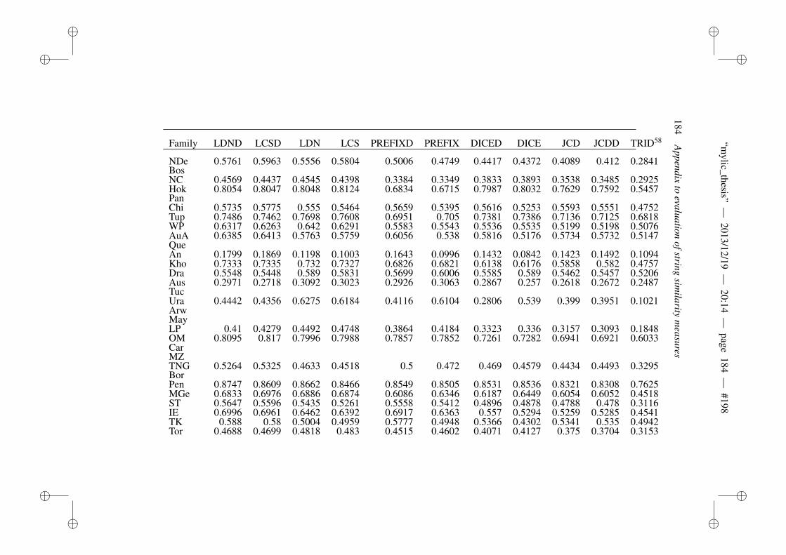
ii

“mylic_thesis”

—2013/12/19

—20:14

—page

184—

#198i

i

ii

ii

184A

ppendixto

evaluationofstring

similarity

measures

Family LDND LCSD LDN LCS PREFIXD PREFIX DICED DICE JCD JCDD TRID58

NDe 0.5761 0.5963 0.5556 0.5804 0.5006 0.4749 0.4417 0.4372 0.4089 0.412 0.2841BosNC 0.4569 0.4437 0.4545 0.4398 0.3384 0.3349 0.3833 0.3893 0.3538 0.3485 0.2925Hok 0.8054 0.8047 0.8048 0.8124 0.6834 0.6715 0.7987 0.8032 0.7629 0.7592 0.5457PanChi 0.5735 0.5775 0.555 0.5464 0.5659 0.5395 0.5616 0.5253 0.5593 0.5551 0.4752Tup 0.7486 0.7462 0.7698 0.7608 0.6951 0.705 0.7381 0.7386 0.7136 0.7125 0.6818WP 0.6317 0.6263 0.642 0.6291 0.5583 0.5543 0.5536 0.5535 0.5199 0.5198 0.5076AuA 0.6385 0.6413 0.5763 0.5759 0.6056 0.538 0.5816 0.5176 0.5734 0.5732 0.5147QueAn 0.1799 0.1869 0.1198 0.1003 0.1643 0.0996 0.1432 0.0842 0.1423 0.1492 0.1094Kho 0.7333 0.7335 0.732 0.7327 0.6826 0.6821 0.6138 0.6176 0.5858 0.582 0.4757Dra 0.5548 0.5448 0.589 0.5831 0.5699 0.6006 0.5585 0.589 0.5462 0.5457 0.5206Aus 0.2971 0.2718 0.3092 0.3023 0.2926 0.3063 0.2867 0.257 0.2618 0.2672 0.2487TucUra 0.4442 0.4356 0.6275 0.6184 0.4116 0.6104 0.2806 0.539 0.399 0.3951 0.1021ArwMayLP 0.41 0.4279 0.4492 0.4748 0.3864 0.4184 0.3323 0.336 0.3157 0.3093 0.1848OM 0.8095 0.817 0.7996 0.7988 0.7857 0.7852 0.7261 0.7282 0.6941 0.6921 0.6033CarMZTNG 0.5264 0.5325 0.4633 0.4518 0.5 0.472 0.469 0.4579 0.4434 0.4493 0.3295BorPen 0.8747 0.8609 0.8662 0.8466 0.8549 0.8505 0.8531 0.8536 0.8321 0.8308 0.7625MGe 0.6833 0.6976 0.6886 0.6874 0.6086 0.6346 0.6187 0.6449 0.6054 0.6052 0.4518ST 0.5647 0.5596 0.5435 0.5261 0.5558 0.5412 0.4896 0.4878 0.4788 0.478 0.3116IE 0.6996 0.6961 0.6462 0.6392 0.6917 0.6363 0.557 0.5294 0.5259 0.5285 0.4541TK 0.588 0.58 0.5004 0.4959 0.5777 0.4948 0.5366 0.4302 0.5341 0.535 0.4942Tor 0.4688 0.4699 0.4818 0.483 0.4515 0.4602 0.4071 0.4127 0.375 0.3704 0.3153

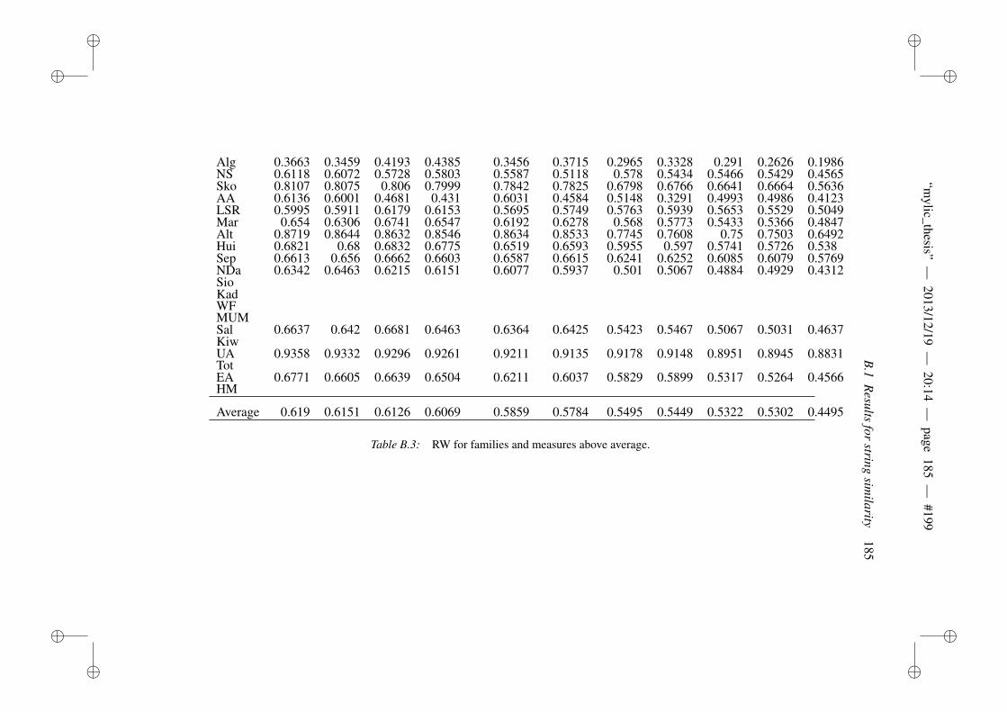
ii

“mylic_thesis”

—2013/12/19

—20:14

—page

185—

#199i

i

ii

ii

B.1

Results

forstring

similarity

185

Alg 0.3663 0.3459 0.4193 0.4385 0.3456 0.3715 0.2965 0.3328 0.291 0.2626 0.1986NS 0.6118 0.6072 0.5728 0.5803 0.5587 0.5118 0.578 0.5434 0.5466 0.5429 0.4565Sko 0.8107 0.8075 0.806 0.7999 0.7842 0.7825 0.6798 0.6766 0.6641 0.6664 0.5636AA 0.6136 0.6001 0.4681 0.431 0.6031 0.4584 0.5148 0.3291 0.4993 0.4986 0.4123LSR 0.5995 0.5911 0.6179 0.6153 0.5695 0.5749 0.5763 0.5939 0.5653 0.5529 0.5049Mar 0.654 0.6306 0.6741 0.6547 0.6192 0.6278 0.568 0.5773 0.5433 0.5366 0.4847Alt 0.8719 0.8644 0.8632 0.8546 0.8634 0.8533 0.7745 0.7608 0.75 0.7503 0.6492Hui 0.6821 0.68 0.6832 0.6775 0.6519 0.6593 0.5955 0.597 0.5741 0.5726 0.538Sep 0.6613 0.656 0.6662 0.6603 0.6587 0.6615 0.6241 0.6252 0.6085 0.6079 0.5769NDa 0.6342 0.6463 0.6215 0.6151 0.6077 0.5937 0.501 0.5067 0.4884 0.4929 0.4312SioKadWFMUMSal 0.6637 0.642 0.6681 0.6463 0.6364 0.6425 0.5423 0.5467 0.5067 0.5031 0.4637KiwUA 0.9358 0.9332 0.9296 0.9261 0.9211 0.9135 0.9178 0.9148 0.8951 0.8945 0.8831TotEA 0.6771 0.6605 0.6639 0.6504 0.6211 0.6037 0.5829 0.5899 0.5317 0.5264 0.4566HM

Average 0.619 0.6151 0.6126 0.6069 0.5859 0.5784 0.5495 0.5449 0.5322 0.5302 0.4495

Table B.3: RW for families and measures above average.

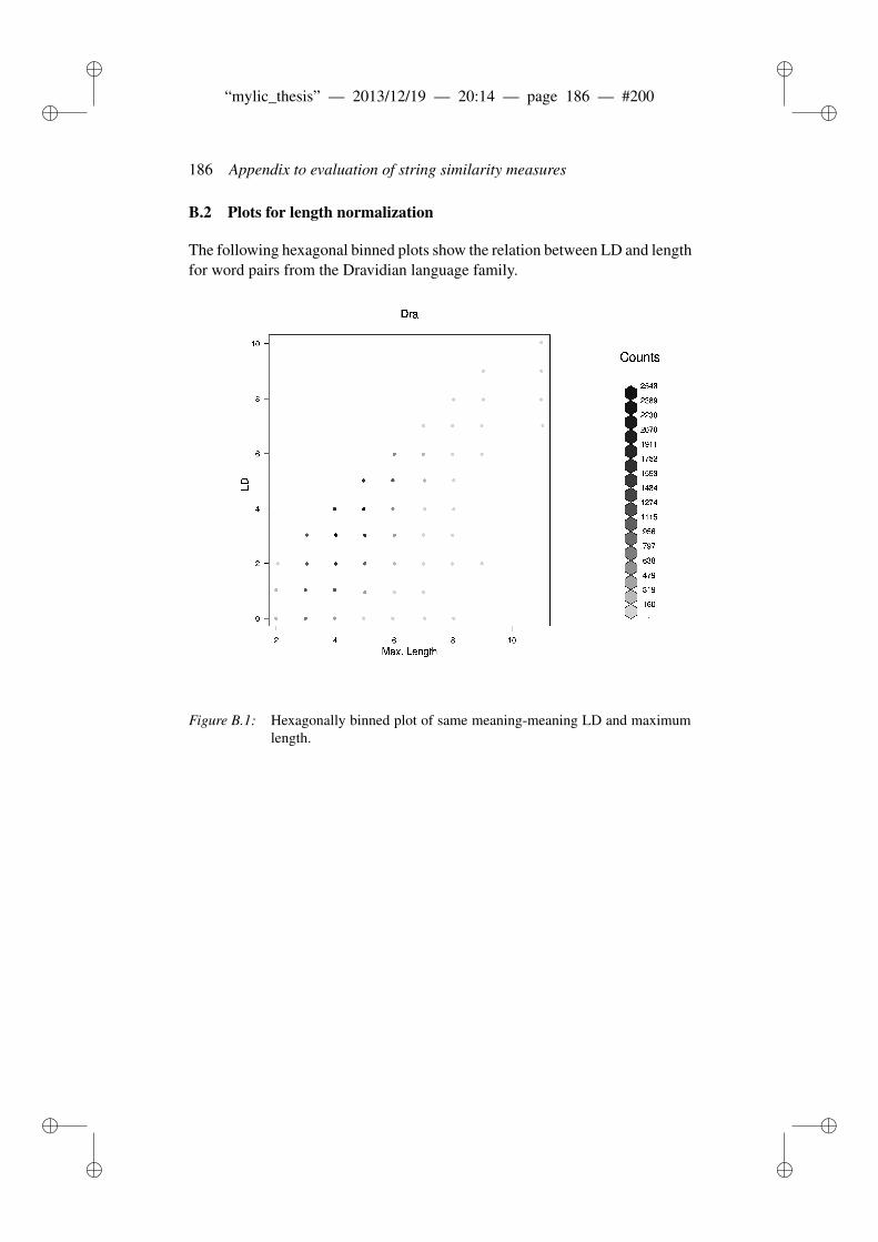
ii


ii

ii

186 Appendix to evaluation of string similarity measures

B.2 Plots for length normalization

The following hexagonal binned plots show the relation between LD and lengthfor word pairs from the Dravidian language family.

Figure B.1: Hexagonally binned plot of same meaning-meaning LD and maximumlength.

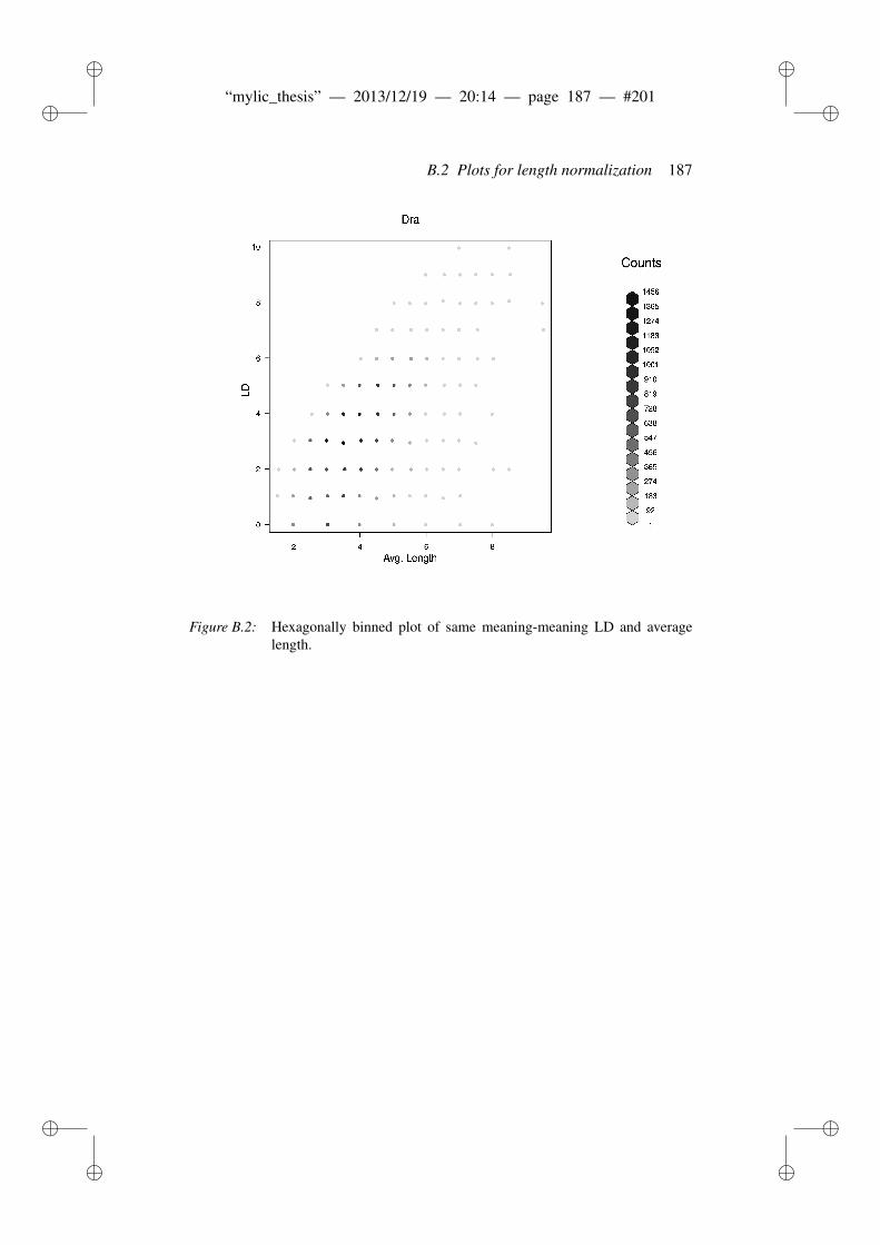
ii


ii

ii

B.2 Plots for length normalization 187

Figure B.2: Hexagonally binned plot of same meaning-meaning LD and averagelength.

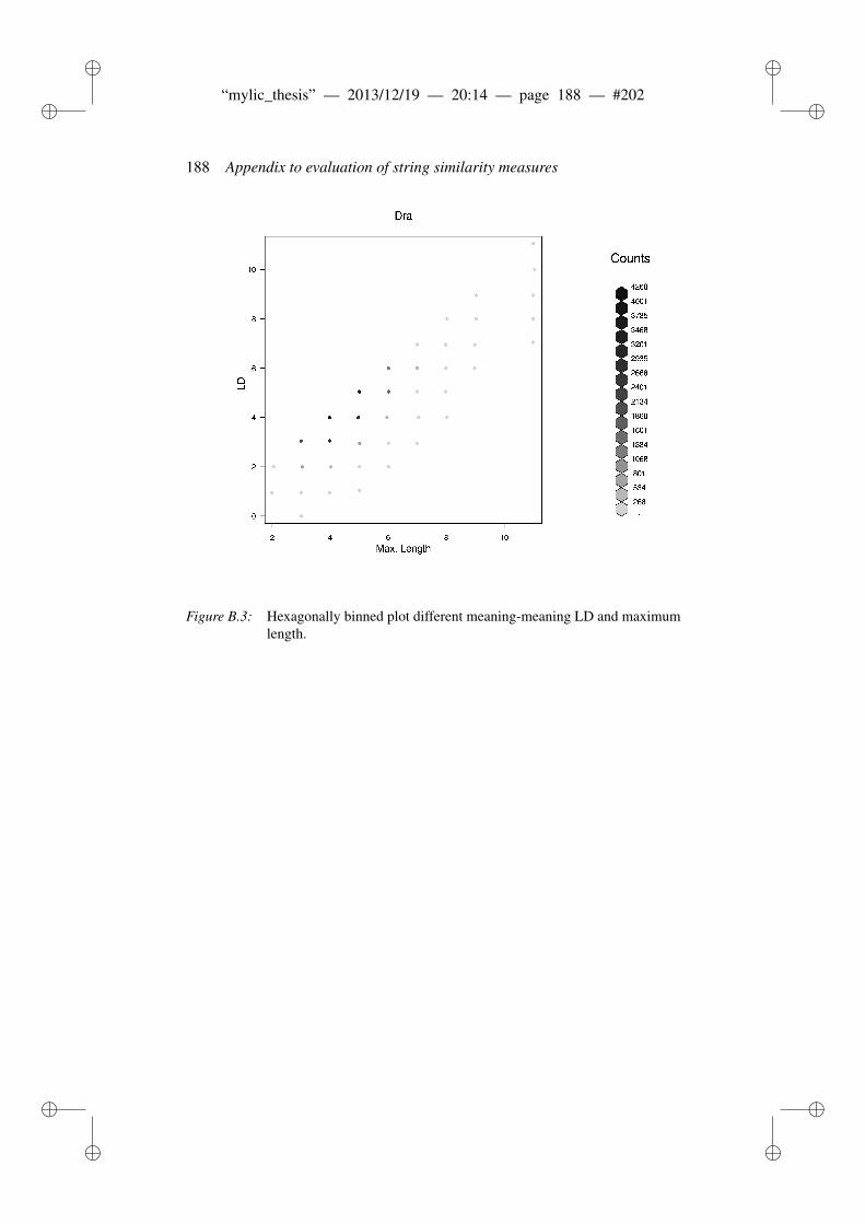
ii


ii

ii

188 Appendix to evaluation of string similarity measures

Figure B.3: Hexagonally binned plot different meaning-meaning LD and maximumlength.

ii


ii

ii

B.2 Plots for length normalization 189

Figure B.4: Hexagonally binned plot different meaning-meaning LD and averagelength.

vocabulary lists in computational historical linguistics

Documents