VALUATION OF TIMBERLANDUNDER PRICE UNCERTAINTY

A DissertationPresented to

the Graduate School ofClemson University

In Partial Ful�llmentof the Requirements for the Degree

Doctor of PhilosophyApplied Economics

byWallace Alexander Campbell

May 2013

Accepted by:Dr. Scott Templeton, Committee Chair

Dr. Tamara CushingDr. R. David LamieDr. James Brannan

Abstract

In the �rst essay, a critical examination of three commonly used stochastic price pro-

cesses is presented. Each process is described and rejected as a possible model of lumber

futures prices. A mean reverting generalized autoregressive conditional heteroskedastic-

ity (GARCH) model, developed by Bollerslev (1986), is proposed as a stochastic process

for lumber futures prices. The essay provides the steps that should be taken to ensure

that a proper price process is used in each application.

In the second essay, a �exible harvesting strategy known as the �reservation price�

strategy is presented. When the current price is below the reservation price, the forest

owner delays the harvest. An optimal stopping model is used to derive an expres-

sion for the optimal sequence of reservation prices under price uncertainty. A solution

method using a Monte Carlo backward recursion algorithm is presented. The Monte

Carlo simulation procedure may be applied when analytical solutions are di�cult or

intractable.

In the third essay, a simulation model is used to estimate the per acre value of

land devoted to timber production under di�erent harvesting strategies, stumpage price

processes, and site qualities. By following the reservation price strategy, forest owners

can increase the expected land value and reduce the variability in land values relative

to a �xed rotation strategy. For an estimated mean reverting GARCH process, the

reservation price strategy increases the value of timberland by 33.0 percent for a site

index of 90 and by 22.1 percent for a site index of 60 relative to a �xed rotation strategy.

ii

Dedication

To my parents, Bill and Janie Campbell, for believing that a Ph.D. in Economics was a

good idea; my grandmother, Edwina Alexander, for suggesting that I choose a topic related

to forestry; Aunt Cheryl and Joe, for not letting me quit; and my friends at Clemson, for

making the whole process highly enjoyable.

iii

Acknowledgements

I would like to thank my committee members for their time, dedication, and willingness

to read revisions on short notice. Special thanks to my advisor, Dr. Scott Templeton, who

met with me for countless hours over the last two years, read and revised thousands of pages,

and who has always been excited about my topics. I also greatly appreciate the help of Dr.

Tamara Cushing with obtaining stumpage prices and simulating timber growth data.

iv

Table of Contents

Page

Title Page . . . . . . . . . . . . . . . . . . . . . . . . . . . . . . . . . . . . . . . . . . . i

Abstract . . . . . . . . . . . . . . . . . . . . . . . . . . . . . . . . . . . . . . . . . . . . ii

Dedication . . . . . . . . . . . . . . . . . . . . . . . . . . . . . . . . . . . . . . . . . . iii

Acknowledgements . . . . . . . . . . . . . . . . . . . . . . . . . . . . . . . . . . . . . . iv

Table of Contents . . . . . . . . . . . . . . . . . . . . . . . . . . . . . . . . . . . . . . . v

List of Tables . . . . . . . . . . . . . . . . . . . . . . . . . . . . . . . . . . . . . . . . . vii

List of Tables . . . . . . . . . . . . . . . . . . . . . . . . . . . . . . . . . . . . . . . . . vii

List of Figures . . . . . . . . . . . . . . . . . . . . . . . . . . . . . . . . . . . . . . . . viii

List of Figures . . . . . . . . . . . . . . . . . . . . . . . . . . . . . . . . . . . . . . . . viii

Chapter 1:Introduction . . . . . . . . . . . . . . . . . . . . . . . . . . . . . . . . . . . . . 11.1 Types of forest owners . . . . . . . . . . . . . . . . . . . . . . . . . . . . . . . 11.2 Objectives of forest owners . . . . . . . . . . . . . . . . . . . . . . . . . . . . . 1

Chapter 2:Choosing a stochastic price process . . . . . . . . . . . . . . . . . . . . . . 42.1 Data . . . . . . . . . . . . . . . . . . . . . . . . . . . . . . . . . . . . . . . . 42.2 Stochastic price models . . . . . . . . . . . . . . . . . . . . . . . . . . . . . . 52.3 Features of observed lumber futures prices . . . . . . . . . . . . . . . . . . . 132.4 Discussion . . . . . . . . . . . . . . . . . . . . . . . . . . . . . . . . . . . . . . 18

Chapter 3:Flexible harvesting strategies in forestry . . . . . . . . . . . . . . . . . . 193.1 Discrete time optimal stopping model . . . . . . . . . . . . . . . . . . . . . . 213.2 The reservation price strategy . . . . . . . . . . . . . . . . . . . . . . . . . . . 233.3 Solving for reservation prices using a backward recursion algorithm . . . . . . 243.4 Advantages of the discrete time model . . . . . . . . . . . . . . . . . . . . . . 313.5 Conclusion . . . . . . . . . . . . . . . . . . . . . . . . . . . . . . . . . . . . . . 32

Chapter 4:What is the value of flexibly harvested timberland? . . . . . . . . . . . 334.1 Stochastic processes for stumpage prices . . . . . . . . . . . . . . . . . . . . . 344.2 Assumptions for numerical simulation . . . . . . . . . . . . . . . . . . . . . . 384.3 Fixed rotation length strategy . . . . . . . . . . . . . . . . . . . . . . . . . . 424.4 Simulation model of land value and harvest dates . . . . . . . . . . . . . . . 42

v

4.5 Simulation results . . . . . . . . . . . . . . . . . . . . . . . . . . . . . . . . . 444.6 Discussion . . . . . . . . . . . . . . . . . . . . . . . . . . . . . . . . . . . . . . 464.7 Barriers and limitations of �exible harvesting strategies . . . . . . . . . . . . 484.8 Application of the model . . . . . . . . . . . . . . . . . . . . . . . . . . . . . . 49

Chapter 5:Conclusion . . . . . . . . . . . . . . . . . . . . . . . . . . . . . . . . . . . . . . . 51

Bibliography . . . . . . . . . . . . . . . . . . . . . . . . . . . . . . . . . . . . . . . . . 52

Appendix . . . . . . . . . . . . . . . . . . . . . . . . . . . . . . . . . . . . . . . . . . . 72

vi

List of Tables

Table Page

1 Net present value, �xed rotation lengths . . . . . . . . . . . . . . . . . . . . . 56

2 Net present value applying the reservation price strategy, site index 60 . . . . 57

3 Net present value applying the reservation price strategy, site index 90 . . . . 58

vii

List of Figures

Figure Page

1 Lumber futures contract prices, monthly averages from November, 1972 toDecember, 2011 . . . . . . . . . . . . . . . . . . . . . . . . . . . . . . . . . . . 59

2 A simulated independent normal price process for lumber futures prices . . . 60

3 A simulated geometric Brownian motion process for lumber futures prices . . 61

4 A simulated geometric Ornstein-Uhlenbeck process for lumber futures prices 62

5 A simulated mean reverting GARCH process for lumber futures prices . . . . 63

6 Normal quantile plot of the distribution of percentage price changes for thesimulated mean reverting GARCH process . . . . . . . . . . . . . . . . . . . 64

7 Squared percentage changes in lumber futures prices (monthly volatility) . . 65

8 Normal quantile plot for monthly percentage changes in lumber futures prices 66

9 Variance ratios for the �rst 100 lags, test tor mean reversion of lumber futures 67

10 Sawtimber volumes for loblolly pine, upstate region of South Carolina, gen-erated using SiMS plantation simulator (ForesTech International, 2006) . . . 68

11 E�ect of price volatility on reservation prices, site index 90 and mean revertingGARCH price process . . . . . . . . . . . . . . . . . . . . . . . . . . . . . . . 69

12 E�ect of site quality on reservation prices, site index 90 and mean revertingGARCH price process . . . . . . . . . . . . . . . . . . . . . . . . . . . . . . . 70

13 Land values from each harvesting strategy, site index 90 and mean revertingGARCH price process . . . . . . . . . . . . . . . . . . . . . . . . . . . . . . . 71

viii

1 Introduction

1.1 Types of forest owners

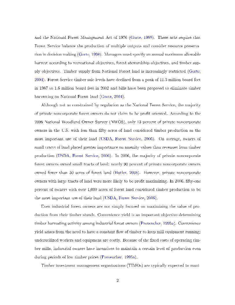
Timberland is de�ned as �forests capable of producing 20 cubic feet per acre of industrial

wood annually and not legally reserved from timber harvest� (Smith et al., 2007). In the

United States, ownership of forest land is classi�ed into four groups: national forest, other

public, private corporate, and private noncorporate. National forest land is managed by

the U.S. Forest Service. In 2007, the Forest Service managed approximately 19 percent of

the forest land in the United States (Smith et al., 2007). The �other public� ownership

class represents forest land managed by the Bureau of Land Management and state and

local governments. These owners managed 11 percent of forest land in 2007 (Smith et al.,

2007). Private corporate forest owners include timber investment management organizations

(TIMOs) and industrial forest owners. Industrial forest owners both manage forest land and

operate wood using plants. Approximately 21 percent of forest land was owned by TIMOs

and industrial corporations in 2007 (Smith et al., 2007). Nonindustrial private forest (NIPF)

owners are a heterogeneous group and have a diverse set of forest management objectives.

Private noncorporate forest owners include individuals and family partnerships. Private

noncorporate owners managed 49 percent of the forest land in the United States in 2007 -

more than any other ownership class (Smith et al., 2007).

1.2 Objectives of forest owners

Of course, timber is not the only output from forest land. To some extent, each ownership

classes uses forest land to produce both timber and non-timber goods. Use of land for

timber production often con�icts with other management objectives, such as scenic value.

In practice, pro�t maximization from timber production does not apply to all forest owners.

Clearly, the management behavior of the National Forest Service is not pro�t maximiz-

ing. Forest managers are highly limited by regulation. Two acts have largely de�ned the

management strategy of the Forest Service: the Multiple-Use Sustained Yield Act of 1960

1

and the National Forest Management Act of 1976 (Gorte, 1998). These acts require that

Forest Service balance the production of multiple outputs and consider resource preserva-

tion in decision making (Gorte, 1998). Managers must specify an annual maximum allowable

harvest according to recreational objectives, forest stewardship objectives, and timber sup-

ply objectives. Timber supply from National Forest land is increasingly restricted (Gorte,

2004). Forest Service timber sale levels have declined from a peak of 11.3 million board feet

in 1987 to 1.6 million board feet in 2002 and bills have been proposed to eliminate timber

harvesting on National Forest land (Gorte, 2004).

Although not as constrained by regulation as the National Forest Service, the majority

of private noncorporate forest owners do not claim to be pro�t oriented. According to the

2006 National Woodland Owner Survey (NWOS), only 13 percent of private noncorporate

owners in the U.S. with less than �fty acres of land considered timber production as the

most important use of their land (USDA, Forest Service, 2006). On average, owners of

small tracts of land placed greater importance on amenity values than revenues from timber

production (USDA, Forest Service, 2006). In 2006, the majority of private noncorporate

forest owners owned small tracts of land: nearly 90 percent of private noncorporate owners

owned fewer than 50 acres of forest land (Butler, 2008). However, private noncorporate

owners with large tracts of land were more likely to be pro�t maximizing. In 2006, �fty-one

percent of owners with over 1,000 acres of forest land considered timber production to be

the most important use of their land (USDA, Forest Service, 2006).

Even industrial forest owners are not simply focused on maximizing the value of pro-

duction from their timber stands. Convenience yield is an important objective determining

timber harvesting activity among industrial forest owners (Provencher, 1995a). Convenience

yield arises from the need to have a constant �ow of timber to keep mill equipment running;

underutilized workers and equipment are costly. Because of the �xed costs of operating tim-

ber mills, industrial owners have incentives to maintain a certain level of production even

during periods of low timber prices (Provencher, 1995a).

Timber investment management organizations (TIMOs) are typically expected to maxi-

2

mize pro�ts from timber production (Binkley et al., 1996). Timberland has become a popular

asset class among investors seeking a stable investment with high dividend yields (Binkley

et al., 1996). With capital from hedge funds, pension funds, and individual investors, organi-

zations such as TIMOs and REITs were formed with the purpose of managing forest land for

pro�t. Through timber harvesting, TIMOs use forest land to generate dividends and capital

gains for shareholders. These nonindustrial corporate owners manage more than half of the

land formerly owned by industrial corporations: as of 2006, TIMOs managed 22.4 million

acres of timberland, worth approximately eighteen billion dollars (USDA, Forest Service,

2011).

Pro�t maximizing agents are most likely to be interested in the topics discussed in this

dissertation. The �rst essay, an analysis of lumber futures prices, primarily applies to large-

scale forest owners that might wish to hedge against timber price risk. The �exible harvesting

strategy presented in the second and third essays re�ects a pro�t maximizing approach to

forest management. The strategy requires active management of timberland speci�cally for

timber production. As a result, the strategy may not coincide with the objectives of the

Forest Service or small-scale, private noncorporate owners. The �exible harvesting strategy

primarily applies to large-scale private noncorporate owners and TIMOs. These owners are

likely to be pro�t maximizing and have the freedom to set rotation intervals without being

restricted by maximum allowable cuts or convenience yield.

3

2 Choosing a stochastic price process

A stochastic process is a sequence of random variables that describes the evolution of

a system over time (Clapham and Nicholson, 2009). Stochastic processes are often used in

dynamic models of uncertainty, including price uncertainty (Dixit and Pindyck, 1994, page

12). The choice of a particular stochastic price process is often critical to the results of the

study. However, many studies in forestry economics have examined the e�ects of �uctuating

prices in forestry without devoting attention to accurately modeling the stochastic price

process (Brazee and Mendelsohn, 1988; Thomson, 1992; Lu and Gong, 2003; Alvarez and

Koskela, 2006, 2007; Manley and Niquidet, 2010). The main objective of this essay is to

provide a price process that can be used for simulation of lumber futures prices and to

describe the steps that should be taken to ensure that a proper price process is used in each

application.

In this essay, three commonly used price processes in forestry economics - independent

draws from a normal distribution, geometric Brownian motion, and the Ornstein-Uhlenbeck

processes - are described and rejected as a price model for lumber futures price data. Mul-

tiple hypotheses are tested regarding features of the price process and distribution of price

changes. A generalized autoregressive heteroskedasticity (GARCH) model, developed by

Bollerslev (1986), is proposed as a stochastic process for prices. GARCH models imply

clustering volatility and heavy tails in the distribution of price changes - features that are

consistent with observed lumber futures prices.

2.1 Data

The monthly average price for random length lumber futures from November, 1972 to

December, 2011 will be used for analysis (Chicago Mercantile Exchange, 2012). Monthly

average prices were calculated from a set of daily opening prices using an algorithm presented

in the Appendix, page 72. There are 470 observations in the monthly average price series.

These prices represent the front month contract for two inch by four inch lumber, eight to

twenty feet long, in dollars per thousand board feet ($/MBF). The front month contract

4

refers to the futures contract with the shortest duration relative to the current date (Chicago

Mercantile Exchange, 2012). Real prices were calculated using the consumer price index

(CPI) as a measure of in�ation (United States Department of Labor, Bureau of Labor

Statistics, 2012). The real price at the beginning of month t is

PRt = Pt ×[CPI0CPIt

], (2.1)

where CPI0 is the value of the CPI in January, 1972 and CPIt is the value of the CPI at

the beginning of month t. The time series of monthly average prices and corresponding real

prices of lumber futures is presented in Figure 1. Here, real prices are in constant January,

1972 dollars.

2.2 Stochastic price models

An overview of three commonly used stochastic processes is presented below. Each

type of price process is characterized by a rational expectations forecast of future prices.

Rational expectations imply that forest owners know the properties of the price process and

forecasts do not systematically deviate from realized prices (Muth, 1961). The parameters

of each model are estimated using lumber futures data and plots of simulated processes are

presented. The computer code for the estimation and simulation of each process is presented

in the Appendix, pages 72 to 74.

2.2.1 Independent draws from a probability distribution

Properties

Consider a price process consisting of a sequence of prices drawn randomly from a �xed

probability density function, f (P ). The distribution function may be discrete or continuous.

Given f (P ) ∼ N(µ, σ2

), an independent normal price process is simulated as

Pt = µ+ σεt, (2.2)

5

where εt ∼ N (0, 1). The rational expectations forecast of the price for an independent price

process is

E [Pt+s|Pt] = µ. (2.3)

The conditional expectation is the same as the unconditional expectation of all future prices;

current and past prices do not a�ect the forecast of future prices. The variance of the process

is σ2. The independence of prices implies that the correlation between Pt and Pt+1 (price

autocorrelation) is zero.

Estimation

The estimated mean and standard deviation for the series of monthly real prices are

µ = 80.0356 and σ = 28.41 dollars per thousand board feet. A simulated series of prices

and the corresponding percentage price changes, using the mean and standard deviation

estimated from the lumber futures data, is presented in Figure 2. The simulation equation

is

Pt = 80.0356 + 28.41εt (2.4)

where P0 = 80.0356 and εtiid.∼ N (0, 1).

2.2.2 Geometric Brownian motion

Properties

Geometric Brownian motion is de�ned by the stochastic di�erential equation

dP = µPdt+ σPdW, (2.5)

where µ is a drift parameter, dt is the change in time, σ is a volatility parameter and

dW = ε (t)×√dt, (2.6)

6

is the increment of a Wiener process (Dixit and Pindyck, 1994, page 71). Here, ε (t) is a

white noise error process assumed to follow a standard normal distribution. In discrete time,

Equation 2.5 can be expressed as

Pt = (1 + µ)Pt−1 + σPt−1εt, (2.7)

where dt = 1 and εtiid.∼ N (0, 1) (Dixit and Pindyck, 1994, page 72). The parameter µ

represents the average (expected) percentage change in prices over one time period and σ

controls the variability of the process.

The conditional forecast of the price is

E [Pt+s|Pt] = Pteµs (2.8)

and the conditional variance of the price is

Var (Pt+s|Pt) = P 2t e

2µs(eσ

2s − 1)

(2.9)

(Dixit and Pindyck, 1994, page 72). When µ = 0, geometric Brownian motion is a martingale

process; the best forecast of all future prices is the current price (Mandelbrot, 1971). Note

that the variance of the process increases over time without bound:

lims→∞

Var (Pt+s|Pt) =∞. (2.10)

As a result, the expected range of prices grows over time.

Estimation

Let

Rt =Pt − Pt−1Pt−1

(2.11)

7

represent the percentage price change from period t− 1 to period t. Note that Equation 2.7

can be expressed as

Rt = µ+ σεt. (2.12)

Consistent parameter estimates for µ and σ are

µ = E [Rt − σεt] (2.13)

= R (2.14)

and

σ = sR (2.15)

where R is the sample mean of R and sR is the sample standard deviation of R. For

the lumber futures prices, the estimated parameters are µ = 0.0005083 and σ = 0.07458.

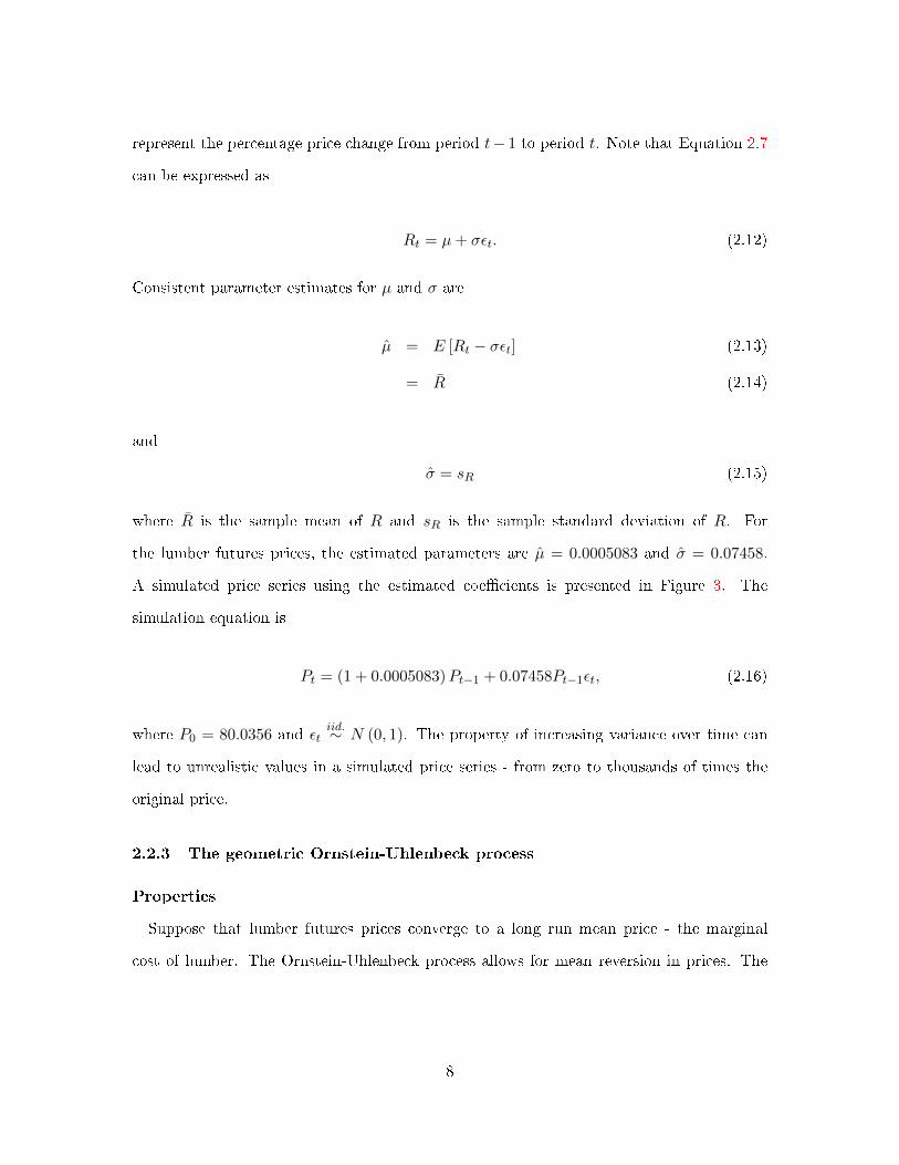
A simulated price series using the estimated coe�cients is presented in Figure 3. The

simulation equation is

Pt = (1 + 0.0005083)Pt−1 + 0.07458Pt−1εt, (2.16)

where P0 = 80.0356 and εtiid.∼ N (0, 1). The property of increasing variance over time can

lead to unrealistic values in a simulated price series - from zero to thousands of times the

original price.

2.2.3 The geometric Ornstein-Uhlenbeck process

Properties

Suppose that lumber futures prices converge to a long run mean price - the marginal

cost of lumber. The Ornstein-Uhlenbeck process allows for mean reversion in prices. The

8

standard Ornstein-Uhlenbeck process is

dP = η (µ− P ) dt+ σdW, (2.17)

where η ≥ 0 measures the speed of mean reversion, µ is the equilibrium price, and dW is the

increment of a Wiener process, de�ned in Equation 2.6 (Dixit and Pindyck, 1994, page 74).

Many applications of stochastic prices in forestry economics have used a variation of the

Ornstein-Uhlenbeck process that allows the volatility of the price to depend upon the price

level (Gjolberg and Guttormsen, 2002; Insley and Rollins, 2005; Insley and Chen, 2012).

The process is de�ned as

dP = η (µ− P ) dt+ σPdW. (2.18)

The process with volatility term σPdW was suggested by Dixit and Pindyck (1994, page

77) and has become known as the �geometric Ornstein-Uhlenbeck process.� An approximate

representation of Equation 2.18 in discrete time is

Pt = Pt−1 + η (µ− Pt−1) + σPt−1εt, (2.19)

where dt = 1 and εtiid.∼ N (0, 1) (Insley and Rollins, 2005). For η = 0, the process is

equivalent to geometric Brownian motion with a drift parameter equal to zero - a random

walk.

The conditional forecast is

E [Pt+s|Pt] = µ+ e−ηs (Pt − µ) . (2.20)

Equation 2.20 implies that if Pt > µ, then E [Pt+1|Pt] < Pt: if the current price is above

µ, the price in the next period is expected to be lower than the current price. For the

geometric Ornstein-Uhlenbeck process, the variability of future prices is a function of the

mean reversion parameter η as well as the volatility parameter σ. The conditional variance

9

of the price s periods into the future is

Var (Pt+s|Pt) =σ2Pt2η

(1− exp (−2ηs)) . (2.21)

An increase in mean reversion (higher value of η) implies a decrease in variance of future

prices:

∂Var [Pt+s|Pt]∂η

=−σ2Pt

2η2+σ2Pt2η2

exp (−2ηs)− 2sσ2Pt2η

exp (−2ηs) < 0. (2.22)

Therefore, the expected range of prices decreases as the level of mean reversion increases.

Lower values for η indicate weaker mean reversion, resulting in a process similar to geometric

Brownian motion. The variance of the process increases over time, but reaches a long-run

limit. The long-run limiting variance of the process is

lims→∞

Var (Pt+s|Pt) =σ2Pt2η

. (2.23)

Estimation

Equation 2.19 can be expressed as

Rt = −η +1

Pt−1ηµ+ σεt, (2.24)

where Rt is de�ned in Equation 2.11. The parameters of the process can be estimated using

the regression

Rt = α+ β1

Pt−1+ et, (2.25)

where α = −η , β = ηµ, and et = σεt (Insley and Rollins, 2005). For the lumber futures

data, α = −0.02376 and β = 1.72750. The estimate σ is the standard deviation of the

regression residuals: σt =√Var (et). The estimated parameters of the geometric Ornstein-

Uhlenbeck process are η = −α = 0.02618 , µ = −β/α = 72.70623, and σ = 0.07419. A

simulated geometric Ornstein-Uhlenbeck process using the estimated coe�cients is presented

10

in Figure 4. The simulation equation is

Pt = Pt−1 + 0.02618 (72.70623− Pt−1) + 0.07419Pt−1εt, (2.26)

where P0 = 72.70623 and εtiid.∼ N (0, 1).

2.2.4 Generalized autoregressive conditional heteroskedasticity models

Properties

Engle (1982) developed a model of asset price changes, known as autoregressive condi-

tional heteroskedasticity (ARCH), to enable �uctuations in price volatility. Unlike geometric

Brownian motion and the geometric Ornstein-Uhlenbeck process, ARCH models allow the

variance parameter to change over time according to an autoregressive model. Building

upon the ARCH model, Bollerslev (1986) developed a generalized ARCH model (GARCH)

where the conditional variance of the process is modeled as an autoregressive moving average

(ARMA) process. The general form of a GARCH (p, q) model is

Pt = E [Pt|Pt−1] + σ2t εt, (2.27)

where εtiid.∼ N (0, 1) and

σ2t = ω +

q∑i=1

αiε2t−i +

p∑i=1

βiσ2t−i (2.28)

(Bollerslev, 1986, page 309). In Equation 2.28, αi represent q autoregressive terms and βi

represent p moving average terms. The conditional expectation term, E [Pt|Pt−1], can repre-

sent any discrete stochastic process including geometric Brownian motion and the geometric

Ornstein-Uhlenbeck process.

The GARCH process can take many di�erent forms. Here, assume that prices follow a

geometric Ornstein-Uhlenbeck process and σt follows an ARMA(1, 1) process. In discrete

11

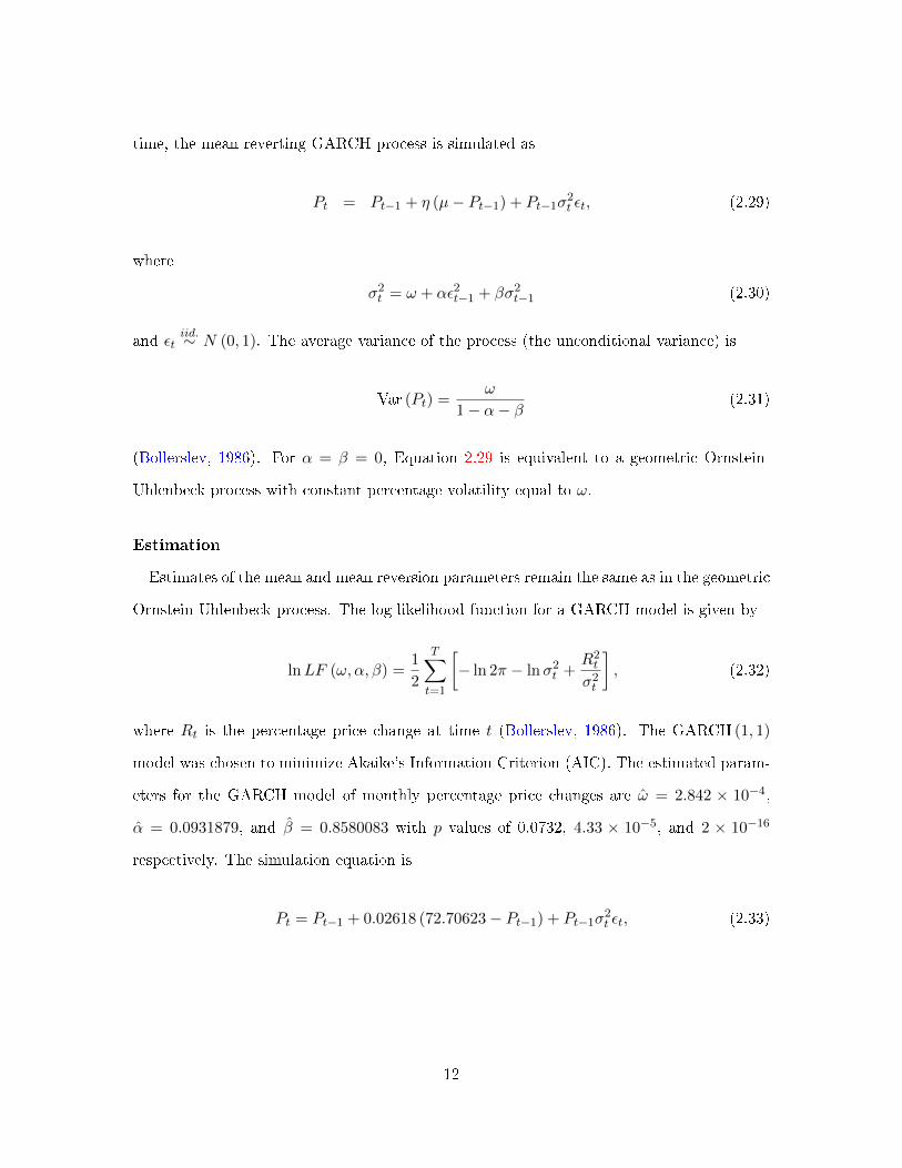
time, the mean reverting GARCH process is simulated as

Pt = Pt−1 + η (µ− Pt−1) + Pt−1σ2t εt, (2.29)

where

σ2t = ω + αε2t−1 + βσ2t−1 (2.30)

and εtiid.∼ N (0, 1). The average variance of the process (the unconditional variance) is

Var (Pt) =ω

1− α− β(2.31)

(Bollerslev, 1986). For α = β = 0, Equation 2.29 is equivalent to a geometric Ornstein-

Uhlenbeck process with constant percentage volatility equal to ω.

Estimation

Estimates of the mean and mean reversion parameters remain the same as in the geometric

Ornstein-Uhlenbeck process. The log-likelihood function for a GARCH model is given by

lnLF (ω, α, β) =1

2

T∑t=1

[− ln 2π − lnσ2t +

R2t

σ2t

], (2.32)

where Rt is the percentage price change at time t (Bollerslev, 1986). The GARCH (1, 1)

model was chosen to minimize Akaike's Information Criterion (AIC). The estimated param-

eters for the GARCH model of monthly percentage price changes are ω = 2.842 × 10−4,

α = 0.0931879, and β = 0.8580083 with p values of 0.0732, 4.33 × 10−5, and 2 × 10−16

respectively. The simulation equation is

Pt = Pt−1 + 0.02618 (72.70623− Pt−1) + Pt−1σ2t εt, (2.33)

12

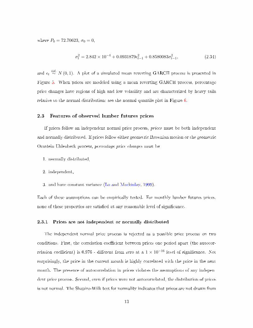
where P0 = 72.70623, σ0 = 0,

σ2t = 2.842× 10−4 + 0.0931879ε2t−1 + 0.8580083σ2t−1, (2.34)

and εtiid.∼ N (0, 1). A plot of a simulated mean reverting GARCH process is presented in

Figure 5. When prices are modeled using a mean reverting GARCH process, percentage

price changes have regions of high and low volatility and are characterized by heavy tails

relative to the normal distribution: see the normal quantile plot in Figure 6.

2.3 Features of observed lumber futures prices

If prices follow an independent normal price process, prices must be both independent

and normally distributed. If prices follow either geometric Brownian motion or the geometric

Ornstein-Uhlenbeck process, percentage price changes must be

1. normally distributed,

2. independent,

3. and have constant variance (Lo and Mackinlay, 1999).

Each of these assumptions can be empirically tested. For monthly lumber futures prices,

none of these properties are satis�ed at any reasonable level of signi�cance.

2.3.1 Prices are not independent or normally distributed

The independent normal price process is rejected as a possible price process on two

conditions. First, the correlation coe�cient between prices one period apart (the autocor-

relation coe�cient) is 0.976 - di�erent from zero at a 1 × 10−16 level of signi�cance. Not

surprisingly, the price in the current month is highly correlated with the price in the next

month. The presence of autocorrelation in prices violates the assumptions of any indepen-

dent price process. Second, even if prices were not autocorrelated, the distribution of prices

is not normal. The Shapiro-Wilk test for normality indicates that prices are not drawn from

13

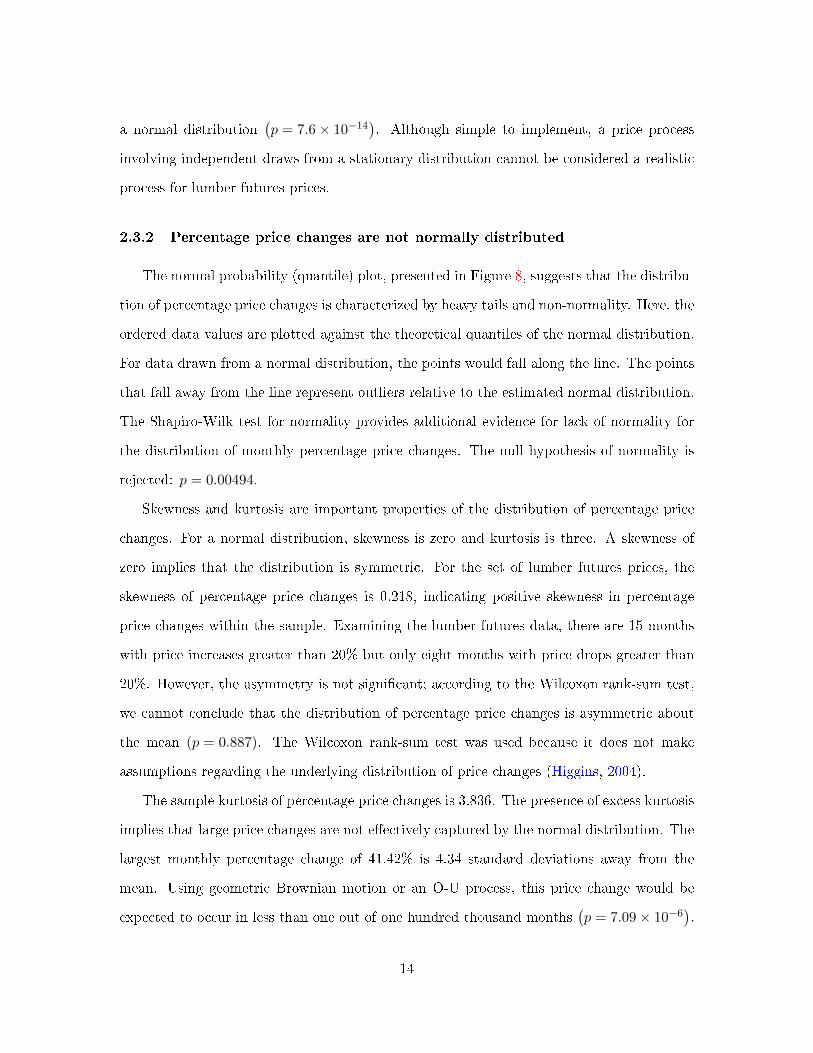
a normal distribution(p = 7.6× 10−14

). Although simple to implement, a price process

involving independent draws from a stationary distribution cannot be considered a realistic

process for lumber futures prices.

2.3.2 Percentage price changes are not normally distributed

The normal probability (quantile) plot, presented in Figure 8, suggests that the distribu-

tion of percentage price changes is characterized by heavy tails and non-normality. Here, the

ordered data values are plotted against the theoretical quantiles of the normal distribution.

For data drawn from a normal distribution, the points would fall along the line. The points

that fall away from the line represent outliers relative to the estimated normal distribution.

The Shapiro-Wilk test for normality provides additional evidence for lack of normality for

the distribution of monthly percentage price changes. The null hypothesis of normality is

rejected: p = 0.00494.

Skewness and kurtosis are important properties of the distribution of percentage price

changes. For a normal distribution, skewness is zero and kurtosis is three. A skewness of

zero implies that the distribution is symmetric. For the set of lumber futures prices, the

skewness of percentage price changes is 0.218, indicating positive skewness in percentage

price changes within the sample. Examining the lumber futures data, there are 15 months

with price increases greater than 20% but only eight months with price drops greater than

20%. However, the asymmetry is not signi�cant; according to the Wilcoxon rank-sum test,

we cannot conclude that the distribution of percentage price changes is asymmetric about

the mean (p = 0.887). The Wilcoxon rank-sum test was used because it does not make

assumptions regarding the underlying distribution of price changes (Higgins, 2004).

The sample kurtosis of percentage price changes is 3.836. The presence of excess kurtosis

implies that large price changes are not e�ectively captured by the normal distribution. The

largest monthly percentage change of 41.42% is 4.34 standard deviations away from the

mean. Using geometric Brownian motion or an O-U process, this price change would be

expected to occur in less than one out of one hundred thousand months(p = 7.09× 10−6

).

14

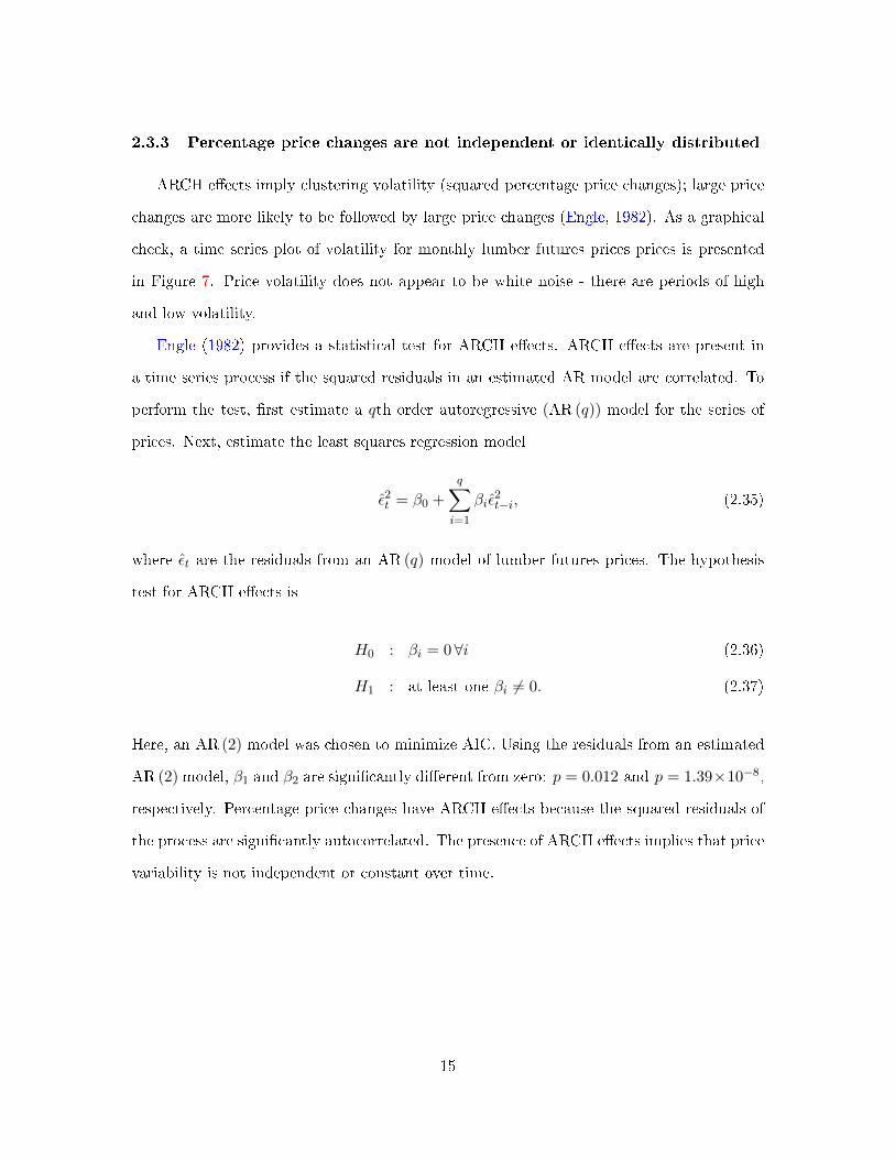
2.3.3 Percentage price changes are not independent or identically distributed

ARCH e�ects imply clustering volatility (squared percentage price changes); large price

changes are more likely to be followed by large price changes (Engle, 1982). As a graphical

check, a time series plot of volatility for monthly lumber futures prices prices is presented

in Figure 7. Price volatility does not appear to be white noise - there are periods of high

and low volatility.

Engle (1982) provides a statistical test for ARCH e�ects. ARCH e�ects are present in

a time series process if the squared residuals in an estimated AR model are correlated. To

perform the test, �rst estimate a qth order autoregressive (AR (q)) model for the series of

prices. Next, estimate the least squares regression model

ε2t = β0 +

q∑i=1

βiε2t−i, (2.35)

where εt are the residuals from an AR (q) model of lumber futures prices. The hypothesis

test for ARCH e�ects is

H0 : βi = 0∀i (2.36)

H1 : at least one βi 6= 0. (2.37)

Here, an AR (2) model was chosen to minimize AIC. Using the residuals from an estimated

AR (2) model, β1 and β2 are signi�cantly di�erent from zero: p = 0.012 and p = 1.39×10−8,

respectively. Percentage price changes have ARCH e�ects because the squared residuals of

the process are signi�cantly autocorrelated. The presence of ARCH e�ects implies that price

variability is not independent or constant over time.

15

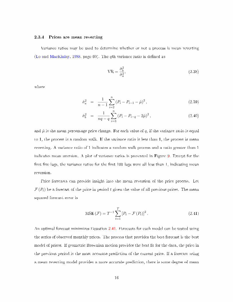
2.3.4 Prices are mean reverting

Variance ratios may be used to determine whether or not a process is mean reverting

(Lo and MacKinlay, 1988, page 60). The qth variance ratio is de�ned as

VR =σ2bσ2a, (2.38)

where

σ2a =1

n− 1

n∑i=2

(Pi − Pi−1 − µ)2 , (2.39)

σ2b =1

nq − q

n∑i=3

(Pi − Pi−q − 2µ)2 , (2.40)

and µ is the mean percentage price change. For each value of q, if the variance ratio is equal

to 1, the process is a random walk. If the variance ratio is less than 1, the process is mean

reverting. A variance ratio of 1 indicates a random walk process and a ratio greater than 1

indicates mean aversion. A plot of variance ratios is presented in Figure 9. Except for the

�rst �ve lags, the variance ratios for the �rst 100 lags were all less than 1, indicating mean

reversion.

Price forecasts can provide insight into the mean reversion of the price process. Let

F (Pt) be a forecast of the price in period t given the value of all previous prices. The mean

squared forecast error is

MSE (F) = T−1T∑t=1

[Pt −F (Pt)]2 . (2.41)

An optimal forecast minimizes Equation 2.41. Forecasts for each model can be tested using

the series of observed monthly prices. The process that provides the best forecast is the best

model of prices. If geometric Brownian motion provides the best �t for the data, the price in

the previous period is the most accurate prediction of the current price. If a forecast using

a mean reverting model provides a more accurate prediction, there is some degree of mean

16

reversion in the price process.

When the historical mean is used as the expected price in the next period, the forecast

error is 5, 893.33. The error when forecasting all future prices as the historical mean is

una�ected by the forecast horizon.Using a random walk forecast, the mean squared error

forecast is 606.51. The mean squared forecast error associated with the mean reverting

forecast is 589.76. The improvement of the mean reverting forecast over the random walk

forecast implies that there is likely some degree of mean reversion in prices. The one month

ahead mean reverting forecast results in an improvement of only 2.81 percent relative to

the martingale forecast. However, when prices are forecast more than one month into the

future, the performance of the mean reverting forecast improves relative to the martingale

forecast. The two, three, and four month ahead mean reverting forecasts provide improve-

ments of 4.98, 7.28, and 9.04 percent, respectively. Clearly, forecasting all future prices as

the historical mean is not the optimal forecast.

Schwartz (1997) and Andersson (2007) present theoretical and empirical evidence for

mean reversion in commodity prices. Andersson (2007) examined the mean reversion of

over 300 commodity futures prices. According to Andersson (2007), �if we believe in the

mechanics of a market economy, prices of standardized goods should in the long-run revert

towards the marginal cost of production as a result of competition among the producers.�

Likewise, in a competitive timber market, the price of a timber should revert to the marginal

cost of production in the long run. If the marginal cost of timber production is constant

over time, lumber futures prices may be expected to to revert to a mean price.

There are three compelling reasons to choose a mean reverting process over geometric

Brownian motion. First, the variance ratios suggest that the process is mean reverting over

time horizons of longer than �ve months. Second, the mean reverting forecast represents an

improvement over the martingale forecast. Third, mean reversion in commodity prices can

be justi�ed and explained on theoretical grounds.

17

2.4 Discussion

Although several studies have examined the common features of a wide range of com-

modity prices (Mandelbrot, 1963; Andersson, 2007), few studies have speci�cally analyzed

lumber futures prices. Insley and Chen (2012) examined the use of a regime switching model

as a process for lumber futures prices. The regime switching model alternated between two

geometric Ornstein-Uhlenbeck processes with di�erent degrees of variability. Insley and

Chen (2012) �nd that the regime switching model provides a better �t for lumber futures

prices than the geometric Ornstein-Uhlenbeck process. However, each regime model requires

percentage price changes to be normally distributed. As demonstrated, processes with nor-

mally distributed percentage price changes provide inadequate models of lumber futures

prices. Additionally, the forest manager must be able to determine when the regime has

switched from a high volatility to a low volatility state.

In this study, several features of lumber futures prices have been identi�ed: price changes

are not normally distributed, price variability is not constant, and prices are mean reverting.

A mean reverting GARCH process can be used to model each of these features. The use

of a ARMA process to characterize the variability of prices relaxes some of the unrealistic

assumptions of geometric Brownian motion and the geometric Ornstein-Uhlenbeck process.

A simulation-based study involving lumber futures prices would require an accurate char-

acterization of the price process. For example, lumber futures could be incorporated into a

�exible harvesting strategy as a method of hedging.

18

3 Flexible harvesting strategies in forestry

The Faustmann model is commonly used to predict the behavior of pro�t maximizing

agents in forestry and to determine the net present value of land devoted to timber pro-

duction. In the Faustmann model, forest owners choose the rotation length - the amount

of time that trees are allowed to grow in between harvests - to maximize the net present

value of land over an in�nite number of timber harvests. The rotation length determines the

harvested volume of timber and the net present value of land devoted to timber production.

Harvesting costs, planting costs, and the timber price are constant and the volume of timber

per acre changes according to a speci�ed deterministic growth function. In a determinis-

tic model with �xed parameters, the optimal rotation length is constant and land value is

known.

In practice, none of the parameters that determine the optimal rotation age are known

with certainty. Fluctuations in prices, costs, interest rates, and timber growth and the

potential for catastrophic losses (forest �res, pest infestations, etc.) cause pro�ts from

future harvests to be uncertain. When any model parameters are stochastic, the value of

land devoted to forestry cannot be expressed with certainty.

In principle, forest managers can time timber harvests in response to changing market

conditions. Forest owners could increase pro�ts by harvesting timber when prices are high

and delaying the harvest when prices are low. Multiple authors have considered the value and

feasibility of �exible harvesting strategies as an alternative to �xing a rotation length at the

time of planting. By using a �exible rotation length, forest owners might avoid uneconomical

harvests in search of higher prices. Norstrom (1975) and Brazee and Mendelsohn (1988)

were among the �rst authors to model a timber harvesting strategy in which forest owners

incorporate price �uctuations into the �nal harvest decision. Each suggested that forest

owners adopt a reservation price harvesting strategy. In each time period, a forest owner sets

a reservation price that depends upon both biological and economic factors. The reservation

price is de�ned as the minimum price in the current period that would induce a forest owner

19

to harvest timber. If the current price is below the reservation price, a forest owner will

delay the �nal harvest. If the current price is above the reservation price, a forest owner will

harvest timber and replant in the current period.

More recent research has adopted the terminology and models used to value �nancial

options (see Thomson, 1992; Plantinga, 1998; Insley and Rollins, 2005; Manley and Niquidet,

2010). An American style �nancial option gives the buyer the right to buy or sell an asset on

or before a speci�ed future date (Dixit and Pindyck, 1994). Planting timber is the equivalent

of purchasing an American put option. By planting trees, the forest owner purchases an

option to sell a growing asset over a range of years. The decision to harvest represents

the exercise of the option. Option value exists in forestry for three reasons. First, timber

harvesting is irreversible. Second, timber harvesting can be delayed; forest owners can

choose to harvest timber over a wide range of years. Third the pro�ts from future timber

harvests are uncertain at the time of planting. Option value would not exist if one or more

of these three conditions were not satis�ed (Dixit and Pindyck, 1994, page 3). Long term

investments are undervalued if option value is ignored (Laughton and Jacoby, 1993; Dixit

and Pindyck, 1994).

Plantinga (1998) described the relationship between option value and the reservation

price strategy: option value is equal to the di�erence between the value of a �xed rotation

length policy and the expected value of a �exible harvesting policy. In the forest economics

literature, option value has been calculated in several ways including the binomial option

pricing model (Thomson, 1992), a discrete time dynamic programming approach (Haight

and Holmes, 1991; Provencher, 1995a; Plantinga, 1998), the Black-Scholes option pricing

model (Hughes, 2000), and continuous time optimal stopping models (Insley, 2002; Insley

and Rollins, 2005; Rocha et al., 2006). In this essay, an discrete time optimal stopping model

20

is used to estimate reservation prices when stumpage prices are stochastic.

3.1 Discrete time optimal stopping model

3.1.1 State and control variables

Timber management can be formulated as a discrete time optimal stopping problem in

which there is a choice to stop (harvest) or continue (delay the harvest) in each period.

Optimal stopping problems are characterized by state variables and control variables (Bert-

sekas, 1987). In each period, the forest owner sets the value of the control variable, de�ned

as

xt =

0 delay the timber harvest

1 harvest timber at the beginning of period t

. (3.1)

The use of a binary control variable implies that the �nal timber harvest is characterized as

an all-or-nothing harvest; partial harvests and thinnings are not considered. Here, assume

that revenues from thinning cancel out any periodic management costs not included in the

model.

Let X be the sequence of harvesting decisions made by the forest owner: X = {xt}∞t=0.

Not all sets of harvesting decisions are possible - for example, the forest owner cannot clear

cut the same plot two periods in a row. Here, the set of feasible controls, X , is de�ned by a

minimum and maximum harvest age.

The state variables represent the information available to the forest owner. The forest

owner decides to harvest or delay harvest in each period based on the values of the state

variables. Here, the state variables are Pt and Vt: the stumpage price and the per acre

volume of merchantable timber at the beginning of period t, respectively. The stumpage

price, P = PH−CH , represents the payment that forest owners receive from a timber �rm in

exchange for the right to harvest standing timber. The stumpage price has two components:

the price of timber, PH , and harvesting costs, CH . Timber prices vary by wood quality and

the forces of supply and demand. Harvesting costs vary by region, tract size, distance from

timber mills, and geography of the tract. All else equal, the stumpage price for a plot of

21

land near a mill will be higher than a plot far away from a mill. The stumpage price is

represented as a discrete stochastic process:

Pt+1 = E [Pt+1|Pt] + εt+1, (3.2)

where εt+1 ∼ N(0, σ2t+1

). Volume is represented as a deterministic function of time:

Vt+1 (xt) = (g (Vt) + Vt) (1− xt) + xt × g (V0) , (3.3)

where g (Vt) is the change in the per acre volume of timber stock that occurs from the

beginning of period t to the beginning of period t + 1. The volume at the beginning of

period t + 1 is a function of the control variable xt. The volume changes according to a

known function that can be estimated from timber stand data.

3.1.2 Model of wealth maximization

Assume that the forest owner's objective is to maximize the discounted stream of payo�s

from an in�nite number of harvest rotations and each rotation begins with tree planting on

bare ground. The forest owner chooses a sequence of harvesting decisions to maximize wealth

from land subject to Equations 3.2 and 3.3. The objective is to de�ne a rule for choosing

the values of the control variable that maximize the wealth of the bare land.

To determine the optimal strategy, the in�nite sequence of rotations can be broken down

into a decision in each quarter. At the beginning of each quarter, forest owners are faced with

two choices: harvest timber or delay the harvest to any future period. At the beginning

of period t, the value of land with planted timber has two components: the value of the

standing timber, PtVt, and the value of bare land, λ. The discounted expected value of

delaying harvest to any future date is de�ned as

βE [J (Pt+1, Vt+1)] , (3.4)

22

where β = 1/ (1 + r/4) is a constant, quarterly discount factor. Equation 3.4 can be inter-

preted as the discounted value of the option to harvest or delay harvest in the next period.

The cost of delaying harvest involves the loss of an interest payment that could have been

earned on harvest revenue as well as the opportunity cost from delaying all future rotations.

The bene�ts of delaying harvest are timber growth and the possibility of a higher price in

the next period.

At the beginning of each period, the forest owner compares the value of the immediate

land value with the discounted expected land value from harvesting in any future period

and chooses between the maximum of the two values. The maximization problem at time t

is

J (Pt, Vt) = max [PtVt + λ, βE [J (Pt+1, Vt+1) |Pt]] . (3.5)

The expected value of delay is equal to the expected discounted value function in the next

period. The Bellman equation for the optimal stopping model is

J (P, V ) = max[PV + λ, βE

[J(P ′, V ′

)|P]], (3.6)

where P ′ and V ′ represent the price and volume at the beginning of the next period. The

function J (P, V ) is known as the �value function� and can be interpreted as the value of

a forest stand with price P and volume V assuming that forest owners follow an optimal

policy in all future periods. The Bellman equation allows the value function to be expressed

independent of time (Bertsekas, 1987).

3.2 The reservation price strategy

A policy consists of a sequence of single-period decision rules that specify the value of the

control variable given the values of the state variables. In the context of forestry, a policy

determines choice to harvest or delay harvest in each period. The forest owner's objective

is to determine the optimal harvest policy.

The problem is similar to the asset sale model presented by Bertsekas (1987), page 78.

23

The optimal policy in asset sale models is to set a reservation price at the beginning of each

period (Bertsekas, 1987). The reservation price policy implies that the control variable is a

function of the current price and current reservation price:

xt (Pt, RPt) =

1 Pt ≥ RPt

0 Pt < RPt

. (3.7)

When the current stumpage price is below the current reservation price, harvest is delayed.

The values of the reservation price and stumpage price determine the optimal decision at

each time period. Under the reservation price strategy, the forest owner can update the

path of the control variable as new price information arrives.

3.3 Solving for reservation prices using a backward recursion algorithm

3.3.1 Assumptions

Backward recursion is commonly used to solve sequential decision processes and has been

widely applied in the forest economics literature (Brazee and Mendelsohn, 1988; Haight and

Holmes, 1991; Plantinga, 1998). To calculate the reservation price using backward recursion,

the Markov property must hold: the future values of the state variables depend only upon

the current values of the state variables, not past values (Dixit and Pindyck, 1994, page 62).

Here, the Markov property implies that the expected value of the price in any future period

depends only upon the current price and the timber volume in all future periods depends

only upon the current timber volume. Additionally, forest owners must know the properties

of the price process and the parameters of the price process must not change over time.

To apply the backward recursion algorithm, a boundary date and value must be de�ned.

Let T be the boundary date. The boundary value at the beginning of period T is equal to

the value of standing timber plus the value of bare land: PTVT + λ. At the beginning of

period T , the forest owner must harvest timber or sell the land with the standing timber -

the value is the same either way. Land will be sold at the current stumpage value plus the

24

value of all future rotations. However, if a forest owner reaches the terminal period without

harvesting, the decision to harvest or sell timber at the beginning of period T may not be

optimal. Therefore, T should be far enough into the future to insure that harvests near T

are highly unlikely.

By de�ning a terminal value, previous value equations can be solved using a backward

recursion algorithm. The boundary value implies that RPT = 0. The goal of the backward

recursion algorithm is to use the information in the terminal period to solve the sequence of

reservation prices RPT−1, RPT−2 . . . RP0.

3.3.2 General solution

Recall the Bellman equation,

J (P, V ) = max[PV + λ, βE

[J(P ′, V ′

)|P]]. (3.8)

In each period, the forest owner sets a reservation price by comparing the value of an im-

mediate harvest with the discounted expected value from delaying the harvest to any future

time period. The reservation price is the value of P that makes the forest owner indi�er-

ent between harvesting at the beginning of the current period and delaying the harvest.

Equating the two values,

PV + λ = βE[J(P ′, V ′

)|P]. (3.9)

Solving Equation 3.9 for P yields the reservation price at the beginning of the current period.

Following the reservation price strategy, a forest owner should harvest at the beginning of

the current period if

P ≥ RP =βE [J (P ′, V ′) |P ]− λ

V, (3.10)

25

where the expected value in the next period is expressed as

E[J(P ′, V ′

)|P, V

]= Pr

(P ′ ≥ RP ′

)×(E[P ′|P ′ ≥ RP ′

]V ′ + λ

)+

(Pr(P ′ < RP ′

)× βE

[J(P ′′, V ′′

)|P ′]). (3.11)

The components of Equation 3.11 can be interpreted as follows.

• Pr (P ′ ≥ RP ′): the probability that timber is harvested at the beginning of the next

period.

• E [P ′|P ′ ≥ RP ′]V ′ + λ: the expected value of a harvest at the beginning of the next

period, given that the price exceeds the reservation price. Because V ′ is known and λ

is assumed to be a constant value, the expectation operator can be distributed. The

conditional price expectation is calculated as

E[P ′|P ′ ≥ RP ′

]=

´∞RP ′ P

′f (P ′|P ) dP ′

1− F (P ′|P ), (3.12)

where f (P ′|P ) is the density function of the stumpage price in the next period con-

ditional on the price in the current period. The calculation of this expectation is

presented in the Appendix, page 74.

• Pr (P ′ < RP ′): the probability that a harvest does not take place at the beginning of

the next period.

• βE [J (P ′′, V ′′) |P ′]: the value of following an optimal strategy in the future if a harvest

does not occur at the beginning of the next period. The expected value of the option

to delay harvest at the beginning of the next period.

Given that

RP ′ =βE [J (P ′′, V ′′) |P ′]− λ

V ′, (3.13)

26

it follows that

E[J(P ′′, V ′′

)|P ′]

=RP ′ × V ′ + λ

β. (3.14)

Therefore, Equation 3.11 can be expressed as

E[J(P ′, V ′

)|P]

= Pr(P ′ ≥ RP ′

)×(E[P ′|P ′ ≥ RP ′

]V ′ + λ

)+ Pr

(P ′ < RP ′

) (RP ′ × V ′ + λ

). (3.15)

This step was essential for computational purposes. By substituting a known reservation

price, calculated in the previous step, recursive calls to the value function were avoided. The

expectation of the value function, E [J (P ′, V ′) |P ], can be solved without the expectation

in the following period, E [J (P ′′, V ′′) |P ′].

3.3.3 Independently and identically distributed normal prices

Assume that the stumpage price in each period is an independent draw from a normal

distribution: Pt ∼ N(µ, σ2

). The value function at the beginning of the �nal period is

J (PT , VT ) = PTVT + λ (3.16)

and the reservation price is RPT = 0. Using these boundary conditions, the sequence of

reservation prices can be found by solving a series of recursive equations starting from period

T − 1 and working backwards. The value function at the beginning of period T − 1 is

J (PT−1, VT−1) = max [PT−1VT−1 + λ, βE [J (PT , VT ) |RPT ]] (3.17)

= max [PT−1VT−1 + λ, β (µ× VT + λ)] . (3.18)

27

Solving the right hand side of Equation 3.18 for PT−1, the reservation price at the beginning

of period T − 1 is

RPT−1 =βE [J (PT , VT ) |RPT ]− λ

VT−1(3.19)

=β (µ× VT + λ)− λ

VT−1. (3.20)

To add one more step, the reservation price at the beginning of the period T − 2 is

RPT−2 =βE [J (PT−1, VT−1) |RPT−1]− λ

VT−2, (3.21)

where the expected value of delaying harvest to period T − 1 is

E [J (PT−1, VT−1) |RPT−1] = (1− Φ (RPT−1))× (E [PT−1|RPT−1]VT−1 + λ)

+ β (Φ (RPT−1)× E [J (PT , VT )]) (3.22)

= (1− Φ (RPT−1))× (E [PT−1|RPT−1]VT−1 + λ)

+ (Φ (RPT−1)×RPT−1VT−1 + λ) . (3.23)

Here, Φ (·) represents the normal cumulative distribution function.

A summary of the steps for the backward recursion algorithm is given below.

1. Write out the value function for period T − 1.

2. Equate the values from harvesting and delaying harvest. Solving for PT−1 yields the

reservation price at the beginning of period T − 1.

3. Calculate the expected value function at the beginning of period T − 1, conditional

upon the value of RPT−1 calculated in step 2.

4. Write out the value function for period T − 2.

5. Equating values and solving for PT−2 yields RPT−2.

28

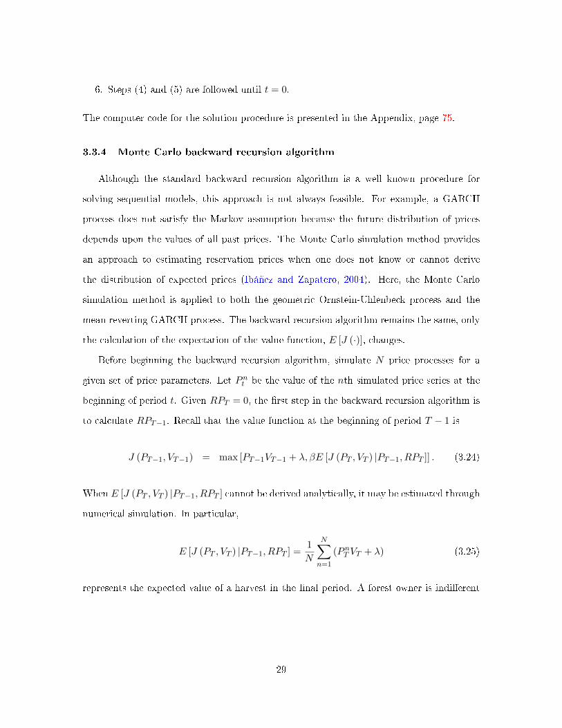
6. Steps (4) and (5) are followed until t = 0.

The computer code for the solution procedure is presented in the Appendix, page 75.

3.3.4 Monte Carlo backward recursion algorithm

Although the standard backward recursion algorithm is a well known procedure for

solving sequential models, this approach is not always feasible. For example, a GARCH

process does not satisfy the Markov assumption because the future distribution of prices

depends upon the values of all past prices. The Monte Carlo simulation method provides

an approach to estimating reservation prices when one does not know or cannot derive

the distribution of expected prices (Ibáñez and Zapatero, 2004). Here, the Monte Carlo

simulation method is applied to both the geometric Ornstein-Uhlenbeck process and the

mean reverting GARCH process. The backward recursion algorithm remains the same, only

the calculation of the expectation of the value function, E [J (·)], changes.

Before beginning the backward recursion algorithm, simulate N price processes for a

given set of price parameters. Let Pnt be the value of the nth simulated price series at the

beginning of period t. Given RPT = 0, the �rst step in the backward recursion algorithm is

to calculate RPT−1. Recall that the value function at the beginning of period T − 1 is

J (PT−1, VT−1) = max [PT−1VT−1 + λ, βE [J (PT , VT ) |PT−1, RPT ]] . (3.24)

When E [J (PT , VT ) |PT−1, RPT ] cannot be derived analytically, it may be estimated through

numerical simulation. In particular,

E [J (PT , VT ) |PT−1, RPT ] =1

N

N∑n=1

(PnT VT + λ) (3.25)

represents the expected value of a harvest in the �nal period. A forest owner is indi�erent

29

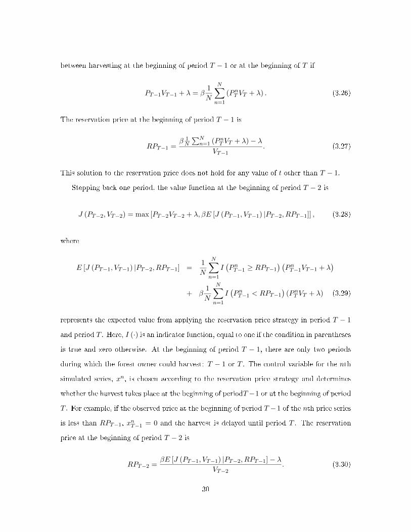
between harvesting at the beginning of period T − 1 or at the beginning of T if

PT−1VT−1 + λ = β1

N

N∑n=1

(PnT VT + λ) . (3.26)

The reservation price at the beginning of period T − 1 is

RPT−1 =β 1N

∑Nn=1 (PnT VT + λ)− λ

VT−1. (3.27)

This solution to the reservation price does not hold for any value of t other than T − 1.

Stepping back one period, the value function at the beginning of period T − 2 is

J (PT−2, VT−2) = max [PT−2VT−2 + λ, βE [J (PT−1, VT−1) |PT−2, RPT−1]] , (3.28)

where

E [J (PT−1, VT−1) |PT−2, RPT−1] =1

N

N∑n=1

I(PnT−1 ≥ RPT−1

) (PnT−1VT−1 + λ

)+ β

1

N

N∑n=1

I(PnT−1 < RPT−1

)(PnT VT + λ) (3.29)

represents the expected value from applying the reservation price strategy in period T − 1

and period T . Here, I (·) is an indicator function, equal to one if the condition in parentheses

is true and zero otherwise. At the beginning of period T − 1, there are only two periods

during which the forest owner could harvest: T − 1 or T . The control variable for the nth

simulated series, xn, is chosen according to the reservation price strategy and determines

whether the harvest takes place at the beginning of periodT−1 or at the beginning of period

T . For example, if the observed price at the beginning of period T −1 of the nth price series

is less than RPT−1, xnT−1 = 0 and the harvest is delayed until period T . The reservation

price at the beginning of period T − 2 is

RPT−2 =βE [J (PT−1, VT−1) |PT−2, RPT−1]− λ

VT−2. (3.30)

30

As t becomes smaller, the calculation of the reservation price becomes increasingly complex

because there are more future periods during which the forest owner could harvest. The

computer code for the Monte Carlo simulation procedure is presented in the Appendix, page

75.

The Monte Carlo simulation procedure was �rst applied in the forestry economics lit-

erature by Petrá�sek and Perez-Garcia (2010) to solve a �exible harvesting problem with

variability in both stumpage prices and carbon prices. The Monte Carlo method does not

require predictions of future prices or price volatility and represents a completely simulated

approach to estimating reservation prices. A drawback to the method is the computational

intensity required to run the simulations. Given that the number of simulations, N , should

be large (at least 5,000), this approach was certainly not feasible for early authors in the

reservation price literature.

3.4 Advantages of the discrete time model

In forestry, discrete time models are more appropriate than continuous time �nancial

option models for several reasons. First, forest owners do not observe prices on a continuous

time scale. Second, there is a limit to the speed of decision making; unlike trading in

�nancial options, a sealed bid auction process cannot be executed instantaneously. NIPF

owners often experience a signi�cant lag between the decision to harvest and the end of

the bidding process (Haight and Holmes, 1991). Third, the time scale can be adjusted - a

daily, monthly, or quarterly model can be derived by changing the parameters of the same

model. Fourth, unlike the binomial option pricing model used by Thomson (1992), the

backward recursion approach allows a full range of prices and a variety of price processes to

be considered. Fifth, discrete time allows a wider range of assumptions to be incorporated

in the same model. For example, di�erent price processes, stochastic discount rates, and

other variables can be considered in the same model. The binomial and Black-Scholes option

pricing models are restrictive in the sense that they both imply that prices are characterized

by geometric Brownian motion.

31

3.5 Conclusion

This study describes a method for applying a �exible harvesting strategy in forestry.

The optimal harvesting strategy is characterized by a reservation (threshold) price: if the

current stumpage price is below the current reservation price, the forest owner delays the

harvest. The sequence of reservation prices can be derived from an optimal stopping model

of the timber harvesting decision. The model implicitly assumes risk neutrality - variability

in wealth does not enter the calculation of the value equation, J (P, V ). Future work should

incorporate landowner preferences into the calculation of a reservation price or reservation

utility.

32

4 What is the value of flexibly harvested timberland?

In this essay, two harvesting strategies are compared: a �xed rotation length policy

and an �exible harvest strategy known as the �reservation price policy.� Both harvesting

strategies require forecasts of prices, costs, interest rates, and timber volumes to estimate

the value of bare land for timber production. The �xed rotation policy ignores the properties

of the stumpage price process and the ability to delay harvest when prices are low. The

�exible harvest policy allows for updating - changing decisions based on new information.

Plantinga (1998) de�ned the increase in net present value from a �exible rotation policy

relative to a �xed rotation policy as a �real option value�. Because option value can never be

negative, the expected pro�ts from a �xed rotation harvesting strategy can never be greater

than the expected pro�ts from a �exible strategy. Therefore, the Faustmann model can be

used to estimate a lower bound on the expected value of a timber investment. Additionally,

the �exible harvest approach shows why forest owners do not abandon timber management

when prices are low - they can delay unpro�table harvests in search of higher pro�ts. When

current prices are low, a �exible harvesting approach may result in a positive net present

value whereas the Faustmann model would suggest that timber management should be

abandoned (Thomson, 1992).

The aim of this study is to use a simulation model to estimate the value of applying a

�exible harvesting strategy. First, assumptions regarding prices and timber growth are pre-

sented. Three types of price processes and two volume functions will be considered. Second,

the value of the �xed rotation length strategy is simulated. Third, optimal reservation prices

are derived using the model presented in the previous essay. A numeric solution procedure

based on Monte Carlo simulation is applied when prices are represented by a geometric

Ornstein-Uhlenbeck process or a mean reverting GARCH process. Fourth, the sequence of

reservation prices is used in a simulation model to estimate the value of land devoted to

timber production. Finally, expected pro�ts from a �xed rotation length policy are com-

pared with the expected pro�ts from a reservation price harvesting strategy. The simulation

33

model indicates that by applying a �exible strategy, a forest owner may be able increase the

net present value of land devoted to timber production relative to a �xed rotation strategy.

4.1 Stochastic processes for stumpage prices

The percentage increase in land value varies greatly for each study and each price process.

The estimated increase in net present value over the Faustmann model ranges from zero

(Clarke and Reed, 1989) to more than six times the Faustmann net present value (Insley and

Rollins, 2005). The calculation of option value is heavily dependent upon the assumptions

of the model - particularly the speci�cation of the stochastic process for stumpage prices.

Manley and Niquidet (2010, page 305) argue that �the sensitivity of results to the underlying

price model is one reason why forest valuers (and their clients) have not adopted option

valuation techniques.�

4.1.1 Independent price process

Early models of stumpage price variability assumed that the stumpage prices were drawn

independently from a known price distribution (Norstrom, 1975; Brazee and Mendelsohn,

1988). Norstrom (1975) used a discrete probability distribution in which prices could move

to one of �ve states in each period. Brazee and Mendelsohn (1988) and Brazee and Bulte

(2000) are among the studies which assume that prices in each period are independent draws

from a normal distribution, Piid∼ N

(µ, σ2

). Each found that the reservation price strategy

greatly increased the value of bare land relative to a �xed rotation strategy. If stumpage

prices are independent draws from a normal distribution, the reservation price strategy

can increase the net present value of timberland by more than 100 percent relative to the

Faustmann model (Brazee and Mendelsohn, 1988). However, the simplistic price models

used by Norstrom (1975) and Brazee and Mendelsohn (1988) are no longer considered to

be reasonable approximations of the true price process. In particular, the assumption that

prices one period apart are uncorrelated is nearly always violated.

34

4.1.2 Geometric Brownian motion

Clarke and Reed (1989), Thomson (1992), Insley (2002), and Manley and Niquidet (2010)

are among the studies that have used geometric Brownian motion as a stochastic process for

prices in a �exible harvesting model. The popularity of geometric Brownian motion stems

from its analytical tractability and its use in the Black-Scholes option pricing model (Black

and Scholes, 1973). Additionally, authors often justify geometric Brownian motion using

market e�ciency arguments. Clarke and Reed (1989), Washburn and Binkley (1990), and

Thomson (1992) argue that the use of geometric Brownian motion is consistent with timber

market e�ciency. In contrast, mean reversion implies that price changes are forecastable.

However, Fama (1970) demonstrates that a price process characterized by geometric Brow-

nian motion is su�cient, but not necessary for market e�ciency. Additionally, McGough

et al. (2004) show that autocorrelated prices can exist in e�cient timber markets given sup-

ply and demand shocks. Therefore, market e�ciency provides no guidance for choosing a

stochastic process for prices.

One drawback to the use of geometric Brownian motion in a simulation study is the

property of increasing price variance over time. To keep prices from becoming zero or

excessively large, the majority of studies using geometric Brownian motion have applied

upper and lower bounds on the prices (Thomson, 1992; Paarsch and Rust, 2004; Manley

and Niquidet, 2010). However, bounding the process results in a process that is no longer

geometric Brownian motion.

Using single rotation models, Clarke and Reed (1989) and Haight and Holmes (1991)

demonstrate that the expected pro�ts from the reservation price strategy and a �xed rotation

length policy are nearly equivalent when prices are characterized by geometric Brownian

motion. In a multiple rotation model incorporating �xed land management costs, Thomson

(1992) demonstrates that the reservation price strategy increases the net present value of land

even when prices are characterized by geometric Brownian motion. According to Thomson

(1992), the increase in the value of land when prices are characterized by geometric Brownian

motion is a result of the ability to delay unpro�table harvests.

35

4.1.3 Mean reverting processes

Mean reverting prices are attractive from a simulation perspective. Unlike geometric

Brownian motion, mean reverting processes do not have the tendency to go to zero or

in�nity over time. Because the variance reaches a long-run limit and the process reverts to

a �xed value, the process stays within what most authors de�ne as a �reasonable� range of

prices - no arti�cial price bounds are required for simulation.

A wide range of studies in forestry have used mean reverting processes to model stumpage

prices. The mean reverting models have included a �rst order autoregressive process (Haight

and Holmes, 1991), the Ornstein-Uhlenbeck process (Plantinga, 1998), and the geomet-

ric Ornstein-Uhlenbeck process (Gjolberg and Guttormsen, 2002; Insley and Rollins, 2005;

Yoshimoto, 2009) to model prices. In the standard Ornstein-Uhlenbeck process, the param-

eter σ represents the absolute volatility of prices, whereas σ represents percentage volatility

in the geometric Ornstein-Uhlenbeck process.

Theoretical arguments have been presented in favor of mean reversion in commodity

prices (Schwartz, 1997). Additionally, empirical evidence has been presented to justify mean

reversion for stumpage prices. Using the variance ratio test developed by Lo and MacKinlay

(1988), Gjolberg and Guttormsen (2002) �nd evidence of mean reversion in stumpage prices

for time intervals greater than one year.

In the forest economics literature, evidence has been presented for both stationarity

(Insley and Rollins, 2005) and nonstationarity of prices (Manley and Niquidet, 2010). Second

order (covariance) stationary implies that the unconditional mean and variance of the price

series do not depend upon t: E [Pt] = µ∀t and Var (Pt) = σ2 ∀t (Hamilton, 1994, page

45). For stationary prices, the expected range and variability of prices are constant. Haight

and Holmes (1991) �nd that monthly prices are stationary and autocorrelated, rejecting the

assumptions of both Brazee and Mendelsohn (1988) (independent normal prices) and Clarke

and Reed (1989) (geometric Brownian motion). However, although stationarity implies mean

reversion, lack of stationarity does not imply that prices are not mean reverting.

Haight and Holmes (1991) were the �rst to demonstrate that the reservation price strat-

36

egy increases pro�ts when prices are mean reverting. For di�erent assumptions, the reserva-

tion price strategy increased pro�ts by 20 to 30 percent relative to a �xed rotation strategy

(Haight and Holmes, 1991). Gjolberg and Guttormsen (2002) demonstrate that the degree

of mean reversion impacts the value of land; stronger mean reversion results in lower land

values because of the reduction in price variability. In contrast with Gjolberg and Guttorm-

sen (2002), Plantinga (1998) found that an increase in mean reversion increases pro�ts from

a �exible harvesting strategy.

4.1.4 Generalized autoregressive conditional heteroskedasticity models

Both geometric Brownian motion and the geometric Ornstein-Uhlenbeck process assume

that percentage price changes are normally distributed with constant mean and variance.

Mandelbrot (1963), Peters (1994), Cont (2001), and others have pointed out the drawbacks

to using a stationary, normal distribution to characterize asset price changes. The use

of a GARCH volatility model relaxes this assumption. GARCH models imply clustering

volatility; large price changes are likely to be followed by large price changes. Additionally,

GARCH models can be used to model heavy tails in the distribution of price changes. Both

features are common to a wide range of commodity prices (Mandelbrot, 1963). GARCH

models have been widely used in �nance, but have not been applied in the forestry option

value literature.

GARCH can be applied as a volatility model for a geometric mean-reverting, or geometric

Ornstein-Uhlenbeck, process. The use of a mean reverting GARCH process allows the

variability of the process to change over time according to an autoregressive moving average

process. Saphores et al. (2002) found that ARCH e�ects were present in four di�erent

monthly time series of stumpage prices. Similarly, Insley (2002) and Insley and Rollins

(2005) found signi�cant ARCH e�ects in monthly stumpage prices and suggested the use of a

GARCH process in future research. However, the GARCH process has not been implemented

in the reservation price literature because of analytical di�culties.

37

4.2 Assumptions for numerical simulation

4.2.1 Stumpage prices

Three stochastic processes for stumpage prices are considered. Two of the processes have

been previously applied in the literature: prices characterized by independent draws from a

normal distribution (Brazee and Mendelsohn, 1988) and the geometric Ornstein-Uhlenbeck

process (Insley, 2002). The use of a mean reverting GARCH process is new to the reservation

price literature.

For pine sawtimber, the mean stumpage price from the �rst quarter of 1992 to the

fourth quarter of 2012 for the upstate region of South Carolina was $317.88 per thousand

board feet and the estimated standard deviation is σ = $74.23 (Timber Mart South, 2012).

Prices were adjusted to constant fourth quarter 2012 prices using the Consumer Price Index

(United States Department of Labor, Bureau of Labor Statistics, 2012). The iid. normal

price process is simulated as

Pt = 317.8848 + 74.23383εt, (4.1)

where εtiid.∼ N (0, 1). For the geometric Ornstein-Uhlenbeck process, stumpage prices are

expected to revert to a long run equilibrium level of $306.15 per thousand board feet. Note

that the estimated long run equilibrium price is not equal to the sample mean of stumpage

prices. The estimated level of mean reversion is η = 0.07192 and the estimated percentage

variance is σ = 0.131. The simulation equation for the geometric Ornstein-Uhlenbeck process

is

Pt = Pt−1 + 0.07192 (306.1527− Pt−1) + 0.131Pt−1εt, (4.2)

where P0 = 306.1527 and εtiid.∼ N (0, 1). The parameters of the GARCH process are

ω = 0.008007, α = 0.3508, and β = 3.44 × 10−18. The simulation equation for the mean

38

reverting GARCH process is

Pt = Pt−1 + 0.07192 (306.1527− Pt−1) + Pt−1σ2t εt, (4.3)

where P0 = 306.1527,

σ2t = 0.008007 + 0.3508ε2t−1 + 3.44× 10−18σ2t−1, (4.4)

and εtiid.∼ N (0, 1).

4.2.2 Timber volume functions

By assumption, the volume of merchantable sawtimber is a deterministic function of

time; volume in every quarter is known with certainty. The yearly volume of loblolly pine

sawtimber was modeled using the SiMS plantation simulator (ForesTech International, 2006).

Quarterly volumes were estimated from yearly simulated data using linear interpolation.

Each site index assumed a planting density of 726 stems per acre and a 90 percent initial

survival rate. For a site index of 90 (base age 25), the stand was thinned to 70 square

feet of basal area per acre at age 12. For a site index of 60 (base age 25), the stand was

thinned to 70 square feet of basal area per acre at age 15. A plot of each timber volume

function is presented in Figure 10. The points represent simulated yearly volumes and the

lines represent interpolated volumes.

4.2.3 Minimum and maximum harvest ages

Sawtimber is de�ned as timber that can be processed into lumber (Cunningham et al.,

2000). Although a tree can be commercially harvested for pulpwood at any time after it

reaches �ve inches diameter at breast height (DBH), forest owners typically delay the saw-

timber harvest until the diameter of trees in a stand are greater than fourteen inches DBH.

At this diameter, trees can be harvested as sawtimber, receiving higher stumpage prices

than timber harvested for pulpwood (Cunningham et al., 2000). Although merchantable

39

timber products exist at younger stand ages, trees cannot be harvested as sawtimber before

a certain age.

In the reservation price model, an exceptionally high price could cause a forest owner to

harvest before timber is mature. To produce sawtimber, the tree must be mature enough

to produce logs with a minimum length of eight feet (Cunningham et al., 2000). Let tmin

represent the date when timber reaches su�cient biological maturity to be harvested as

sawtimber. Before the beginning of period tmin, timber can only be harvested for pulpwood.

The value of tmin depends upon the species of tree and the productivity of the land. On a

high quality site managed for timber production, loblolly pine trees will require a minimum

of 25 years to be harvested as quality sawtimber (Cunningham et al., 2000). For a site index

of 90, tmin = 25 years (100 quarters). For a site index of 60, tmin = 30 years (120 quarters).

For t < tmin, the reservation price is set to in�nity - no stumpage price can induce a forest

owner to harvest.

Derivation of the reservation price using the backward recursion algorithm requires the

speci�cation of a maximum harvest date, tmax. Here, the maximum harvest date (the

expiration of the option) re�ects the date beyond which signi�cant decline in the timber

stock begins to occur (Gjolberg and Guttormsen, 2002). Beyond tmax, timber may lose value

from mortality. Although the volume functions used in this study do not have a region of

declining timber stock, an arti�cial boundary needs to be set. Here, the maximum harvest

age is set to 50 years (200 quarters) for a site index of 90 and 65 years (260 quarters) for a

site index of 60. Although the choice is somewhat arbitrary, the maximum harvest date can

be chosen to be su�ciently far into the future so that the probability of a harvest near tmax

is nearly zero. Although the reservation price declines sharply to zero near tmax, reservation

prices over the majority of the rotation interval are not sensitive to the speci�cation of the

maximum harvest date. Additionally, the simulation model demonstrates that forest owners

will not harvest near tmax given an optimal series of reservation prices.

40

The constraint requiring minimum and maximum harvest ages can be expressed as

xt =

0 t < tmin

0, 1 tmin ≤ t < tmax

1 t = tmax

, (4.5)

where xt = 0 represents the decision not harvest at the beginning of period t. The minimum

and maximum harvest ages de�ne the set of feasible controls, X .

4.2.4 The value of bare land

The value of bare land, λ, is a random variable that is endogenous to the calculation

of the reservation price. Applying the reservation price strategy a�ects the initial value of

land, which in turn, a�ects the calculation of reservation prices. Land should be valued not

at the constant rotation value, but at the expected value using a �exible harvesting strategy.

An iterative procedure can be used to solve for λ. The lower bound on the value of

bare land can be estimated using a discrete version of the Faustmann model. The discrete

Faustmann model speci�es that the net present value of timber land with an in�nite number

of rotation intervals, each of length t, is

NPV (t) =βtPtVt − Cp

1− βt, (4.6)

where Cp represents planting costs (assumed to be constant) (Kennedy, 1986). Equation

4.6 can be maximized by solving the equation for t = tmin, tmin+1, . . . , tmax and �nding the

maximum net present value out of all possible choices of t. The solution to Equation 4.6

provides the starting value for λ in the simulation model.

This study will assume that the expected value of bare land is equal to a long-run

expected value that does not depend upon the current price level. The forecast of a mean

reverting random variable more than 100 quarters into the future is approximately the mean

of the process. Therefore, when prices are mean reverting, λ does not depend upon the price

41

at the time of planting. For additional details in support of removing the dependence of

land value on the current stumpage price level, see Brazee and Mendelsohn (1988), Haight

and Holmes (1991), Provencher (1995a), and Plantinga (1998). Although λ is not time-

dependent, it depends upon the assumptions of the model.

4.3 Fixed rotation length strategy

The reservation price strategy will be compared relative to the value of a �xed rotation

strategy. For a �xed rotation length strategy, the forest owner chooses a rotation length to

maximize the expected net present value of land. Given constant prices and planting costs,

all rotation lengths will be the same. Harvesting at the Faustmann optimal rotation length

is one possible harvesting policy. Let t? be the rotation length that maximizes Equation 4.6

given a price equal to the mean of the process. The policy implies that

xt (t?) =

1 t = t?, 2t?, . . .

0 otherwise

. (4.7)

This rotation policy is determined according to information available in the initial time

period and without regard to the distribution of prices or the stumpage price at each harvest

date. Following a constant rotation strategy, the expected value of bare land is

E [NPV (t?)] =βt

?E [Pt? ]Vt? − Cp

1− βt?. (4.8)

The computer code for the discrete Faustmann model is presented in the Appendix, page

75.

4.4 Simulation model of land value and harvest dates

Application of the backward recursion algorithm yields a single estimate of the value

of bare land: E [λ]. To determine the variability in land values that forest owners can

expect from applying the reservation price strategy, a simulation model was developed. This

42

simulation model calculates the pro�ts from applying the reservation price strategy over a

period of 1,000 quarters (250 years). For any reasonable discount rate, timber harvest pro�ts

beyond 250 years into the future become negligible (less than 0.01%) relative to harvesting

pro�ts from earlier rotations. The simulation method is described in the following steps and

the computer code is presented in the Appendix, page 78.

1. Simulate a price series for a given set of parameters starting with the same initial

conditions: P0 = µ and V0 = 0. Start with the Faustmann model estimate of the value

of bare land, λ.

2. Solve for the set of optimal reservation prices using the backward recursion algorithm.

3. Apply the reservation price strategy to each price series. The optimal harvest date, t?,

is de�ned as the smallest value of t for which the simulated stumpage price is greater

than the reservation price:

t? = min [t|Pt ≥ RPt] . (4.9)

4. After timber is harvested, the volume function is reset to zero.

5. Repeat steps three and four until the end of 1,000 quarters. At the end of the simula-

tion, each harvest pro�t is discounted by the appropriate factor and summed, providing

a single net present value. for each simulation. The net present value for each sim-

ulation is equivalent to the discounted value of managing timber according to the

reservation price strategy for 1,000 quarters.

6. Repeat steps one through �ve 10,000 times.

7. The average value of bare land is from the 10,000 simulations is used as the new

estimate of the expected value of bare land. Repeat steps one through six using the

updated value of bare land. After λ is updated a single time, subsequent changes in

bare land are very small - less than 0.1 percent of total land value.

43

This method generates a di�erent net present value and multiple rotation lengths for each

price simulated price process. The expected outcomes are the mean of the net present value

and the mean of the simulated rotation lengths for all 10,000 simulations. The standard

deviation is used as the measure of variability for both variables. The net present value from

the simulation model represents the per acre pro�t of timberland with speci�ed character-

istics, starting with a price equal to the mean of the process. For 10,000 simulations, the

method is stable - land values change by less than a tenth of a percent when the simulation

algorithm is repeated.

4.5 Simulation results

4.5.1 Expected land value under a �xed rotation length strategy

Fixed rotation length harvest values are calculated using a simulation model presented

in the Appendix 80. All simulations used a discount rate of r = 0.05 and planting costs of

$250 per acre. If prices are draws from an independent normal distribution, the expected

value of the price at any future date is $317.8848 per thousand board feet. If prices follow a

mean reverting process, the expected long-run price is $306.1527 per thousand board feet. In

each case, the optimal constant rotation length is 124 quarters (31 years) for a site index of

90 and 174 quarters (43.5 years) for a site index of 60. Here, the rotation length re�ects the

amount of time that timber is allowed to grow for the production of sawtimber. The change

in the expected price was not large enough to a�ect the discrete rotation length. Other

timber products (pulpwood and chip and saw) would have much shorter rotation lengths.

A summary of the results for the constant rotation strategy is presented in Table 1. Ten

thousand simulations were conducted for each set of price process and volume parameters.

Here, E [NPV] represents the mean net present value of the 10,000 simulations(E[λ])

and√Var (NPV) is the standard deviation of the simulated land values. Under the constant

rotation length strategy, an increase in price variability increases the standard deviation of

simulated land values but does not change the expected land value.

44

4.5.2 Applying the reservation price harvesting strategy

Selected results for di�erent price processes and parameters are presented in Tables 2

and 3. Here, E [t?] represents the mean harvest date when applying the reservation price

strategy and√Var (t?) is the standard deviation of the simulated harvest dates.

Result 4.5.1. The reservation price strategy increases the value of timberland relative to a

�xed rotation strategy.

Applying the reservation price strategy, a forest owner would typically harvest at prices

above the mean of the price process. For all chosen parameters of each price process, the

reservation price strategy increased the value of land devoted to timber production. For the

estimated parameters of each price process, the net present value of land increased between

22.1 and 70.3 percent, depending upon the price process and site index of the land. When

prices are independent draws from a normal distribution, the reservation price strategy

increases the value of land by 48.0 percent for a site index of 90 and by 70.3 percent for

a site index of 60. When prices follow a geometric Ornstein-Uhlenbeck process with �xed

volatility, the reservation price strategy increases the value of land by 28.3 percent for a site

index of 90 and by 41.4 percent for a site index of 60. When prices follow a mean reverting

GARCH process, the reservation price strategy increases the value of land by 33.0 percent

for a site index of 90 and by 22.1 percent for a site index of 60.

Result 4.5.2. The reservation price strategy decreases the standard deviation of land values

relative to land values from a �xed rotation strategy.

For the GARCH model with estimated parameters and a site index of 90, the standard

deviation of land values decreases from 27.5 percent of the expected land value under a

�xed rotation strategy to 16.3 percent of the expected land value under the reservation price

strategy. For a site index of 60, the standard deviation of land values decreases from 45.1

percent of the expected land value under a �xed rotation strategy to 18.1 percent of the

expected land value under the reservation price strategy.

45

Result 4.5.3. As stumpage price variability increases, the gains from a �exible harvesting

strategy increase.

For the mean reverting GARCH process and a site index of 90, a 25 percent increase in

σt led to an increase in simulated land value of 30.2 percent relative to the �xed rotation

length strategy. A 25 percent decrease in σt led to an increase in simulated land value of

only 13.5 percent relative to the estimated process. For a site index of 60, a 25 percent

increase in σt led to an increase in simulated land value of 44.8 percent relative to the �xed

rotation length strategy. A 25 percent decrease in σt led to an increase in simulated land

value of only 19.8 percent relative to the estimated process.

Result 4.5.4. The reservation price strategy has a greater impact on land value for lower

quality sites.

The reservation price strategy has a greater positive impact on the value of timberland

with a lower site index. For the estimated mean reverting GARCH process, the reservation

price strategy increases the value of land by an additional 10.9 percent for a site index of 90

relative to a site index of 60.

4.6 Discussion

4.6.1 Properties of reservation prices

A number of general properties of reservation prices hold regardless of the stochastic

process of stumpage prices. First, the optimal reservation prices are not a constant over

the rotation. The value of delaying the harvest decreases over time because there are fewer

periods during which the option can be exercised. Therefore, J (P, V ) ≥ J (P ′, V ′), which

implies that reservation prices must decrease over the rotation interval. Additionally, the

decrease in the reservation price over the rotation interval re�ects the decrease in timber

growth relative to timber volume over time. The reservation price is higher for early stages

of each rotation but decreases as timber growth slows. Second, the reservation price sharply

declines to zero as t approaches tmax. At the maximum harvest age, forest owners will, by

46

assumption, sell timber at the going rate; there is little value to delaying harvest in search of

higher prices. However, harvests near tmax are extremely rare. In the model with estimated

price parameters and 10,000 simulations, no harvests occurred at t = tmax.

Changes in exogenous variables have a consistent e�ect upon reservation prices regardless

of the stochastic process of stumpage prices and the site index. First, site quality impacts

the reservation price. For a high quality site, timber growth imposes a greater penalty for

delaying harvest, resulting in lower reservation prices (Figure 12). Second, greater price

variability increases reservation prices (Figure 11).

4.6.2 Stumpage price volatility

Greater price volatility increases the value of real options because it allows the holder

of the option the ability to sell at a wider range of prices (Laughton and Jacoby, 1993;

Dixit and Pindyck, 1994). Likewise, previous studies of real option value in forestry have

found that higher levels of stumpage price volatility increase the value of �exible harvesting

strategies(Thomson, 1992; Insley, 2002). In this study, an increase in price volatility leads

to an increase in the net present value of land, implying that forest owners bene�t from

greater stumpage price volatility. An increase in price volatility also increases the variability

in simulated land values.

4.6.3 Variability in land values

Previous studies of �exible harvesting strategies in forestry have only estimated the ex-

pected net present value of land devoted to timber production. The simulation model pre-

sented in this study allows for the analysis of the variability of land values. Here, variability

refers to the standard deviation of simulated land values.

When forest owners follow a constant rotation policy, all of the variability in pro�ts from

timber harvesting comes from price volatility. Here, the volume at the optimal rotation

length is assumed to be known. Applying the reservation price strategy introduces harvest

volume variability because not all harvests occur at the same rotation length. However,

47

variability in harvest prices is greatly reduced. By choosing not harvesting at low stumpage

prices, forest owners harvest over a smaller range of prices. The overall e�ect is a reduction

in the variance of pro�ts. Although a risk neutral forest owner is not concerned with pro�t

variability, risk averse forest owners have an additional incentive to apply the reservation

price strategy. A density plot of simulated pro�ts for the �xed rotation length strategy and

reservation price strategy is presented in Figure 13. The reservation price strategy increases

simulated pro�ts and decreases the spread of simulated pro�ts relative to the �xed rotation

length strategy.

4.6.4 E�ects of GARCH volatility

The mean reverting GARCH model allows for a more �exible estimation of the volatility

parameter in the geometric Ornstein-Uhlenbeck process. The stochastic volatility compo-

nent for prices impacted the net present value of land relative to the geometric Ornstein-

Uhlenbeck process. For a site index of 90, the expected net present value of land was

5.5 percent lower than the value when prices were modeled using a geometric Ornstein-

Uhlenbeck process. For a site index of 60, the decrease in expected net present value was

5.4 percent. Additionally, the mean reverting GARCH model impacted the variability of

expected pro�ts relative to the geometric Ornstein-Uhlenbeck process. For a site index of

90, the standard deviation of expected pro�ts decreased from $509.01 under the geometric

Ornstein-Uhlenbeck process to $441.13 when prices follow a mean reverting GARCH pro-

cess. Likewise, for a site index of 60, the standard deviation of expected pro�ts decreased

from $124.56 under the geometric Ornstein-Uhlenbeck process to $112.46 when prices follow

a mean reverting GARCH process.

4.7 Barriers and limitations of �exible harvesting strategies

4.7.1 Selection and estimation of the price process

Land valuation using the reservation price strategy is sensitive to the price process and

the parameter estimates for each process. The use of an unrealistic stochastic process for

48

prices can overvalue land. In this study, modeling prices with an independent normal price

process results in a 27.1 percent greater land valuation than when prices are characterized

by a mean reverting GARCH process. If the stumpage price in the current month is cor-

related with the stumpage price in the next month, the assumption that stumpage prices

are independent draws from a normal distribution is incorrect. The correlation of stumpage

prices one quarter apart, 0.86, suggests that the independent normal price process is not

a reasonable process for stumpage prices. If prices followed an independent price process,

price autocorrelation would be nearly zero. Additionally, the parameters of the price pro-

cess could change over time, re�ecting changes in the timber market. The reservation price

strategy presented in this study relies upon a de�ned (known) stochastic process for prices.

If the mean or volatility of prices changes over time, harvest value calculations could be

misleading.

4.7.2 Costs of price monitoring and imperfect price information

Although forest owners can attempt to harvest more timber during periods of high prices

and harvest less timber during periods of low prices, a variety of barriers exist that may

limit the success of market timing. First, measuring stumpage prices is costly. Forest

owners can obtain price information through a consulting forester or through a variety of

proprietary timber market information services. Provencher (1995b) argues that a simple

rotation length model may be appropriate if price information is costly. Fixed rotation

lengths have an advantage of eliminating the costs of price monitoring (Haight and Holmes,

1991). Second, price measurement is imperfect. Regional average prices provided by timber

market services mask signi�cant variation in local prices. The stumpage price that a forest

owner actually receives can vary depending on location and quality.

4.8 Application of the model

The simulated results apply to a single timber product in the upstate region of South

Carolina, with speci�c site characteristics. For the estimated parameters of the mean re-

49

verting GARCH process, the gains from following an optimal �exible management strategy

range from 22 to 33 percent relative to the net present value under a �xed rotation strategy.

Over all assumptions tested, the range of land values is much larger: from 13 to 70 percent

larger than the value of a �xed rotation strategy. This suggests that accurate calibration of

the model is critical to the results. For each application, the model should be customized

for a speci�c plot by incorporating di�erent volume functions and a price process estimated

from local stumpage price data.

50

5 Conclusion

The �rst essay discusses an optimal simulation model for lumber futures prices. The

mean reverting GARCH process provides a model that could be used in a study concerned

with hedging the value of forest assets. Combined with the model of reservation prices in the

second essay, the simulation model presented in the third essay can be applied directly to

the valuation of timberland. The simulated results suggest that forest owners can increase

timber harvesting pro�ts and decrease the variability in pro�ts by following an optimal

strategy. The estimation of land value when stumpage prices are characterized by a mean

reverting GARCH is new to the forestry option value literature.

Each essay has broader applicability than the �eld of forestry economics. The �rst

essay highlights common characteristics of commodity prices: price volatility changes over

time and the distribution of percentage price changes has heavy tails relative to a normal

distribution. The arguments for the use of a mean reverting GARCH process applies to all

�elds where a stochastic process must be used to model uncertainty, especially �uctuations

in commodity prices. The decision model and simulation procedures in the second and third

essays have applications in all areas of natural resource management. Many types of resource

extraction problems can be viewed as an choice to extract the resource in the current period

for a certain price or delay extraction and face uncertain prices.

51

Bibliography

Alvarez, L. H. R., Koskela, E., 2006. Does risk aversion accelerate optimal forest rotationunder uncertainty? Journal of Forest Economics 12, 171�184. 4

Alvarez, L. H. R., Koskela, E., 2007. Optimal harvesting under resource stock and priceuncertainty. Journal of Economic Dynamics and Control 31, 2461�2485. 4

Andersson, H., 2007. Are commodity prices mean reverting? Applied Financial Economics17, 769�783. 17, 18

Bertsekas, D. P., 1987. Dynamic Programming: Deterministic and Stochastic Models. En-glewood Cli�s, NJ: Prentice Hall, Inc. 21, 23, 24

Binkley, C. S., Raper, C. F., Washburn, C. L., 1996. Institutional ownership of US tim-berland: History, rationale, and implications for forest management. Journal of Forestry94 (9), 21�28. 3

Black, F., Scholes, M., 1973. The pricing of options and corporate liabilities. Journal ofPolitical Economy 81, 637�659. 35

Bollerslev, T., 1986. Generalized autoregressive conditional heteroskedasticity. Journal ofEconometrics 31, 307�327. ii, 4, 11, 12

Brazee, R. J., Bulte, E., 2000. Optimal harvesting and thinning with stochastic prices. ForestScience 46(1), 23�31. 34

Brazee, R. J., Mendelsohn, R., 1988. Timber harvesting with �uctuating prices. ForestScience 34(2), 359�372. 4, 19, 24, 34, 36, 38, 42

Butler, B. J., 2008. Family forest owners of the United States, 2006. In: Newtown Square,PA: USDA Forest Service, Northern Research Station. 2

Chicago Mercantile Exchange, February 2012. Random length lumber futures. http://www.cmegroup.com. 4, 5

Clapham, C., Nicholson, J., 2009. Concise dictionary of mathematics. Oxford UniversityPress. 4

Clarke, H. R., Reed, W. J., 1989. The tree cutting problem in a stochastic environment: Thecase of age-dependent growth. Journal of Economic Dynamics and Control 13, 569�595.34, 35, 36

Cont, R., 2001. Empirical properties of asset returns: Stylized facts and statistical issues.Quantitative Finance 1, 223�236. 37

Cunningham, K., Barry, J., Walkingstick, T., 2000. Managing loblolly pine stands... from Ato Z. University of Arkansas Cooperative Extension Service, FSA5023. 39, 40

Dixit, A. K., Pindyck, R. S., 1994. Investment Under Uncertainty. Princeton, NJ: PrincetonUniversity Press. 4, 7, 9, 20, 24, 47

52

Engle, R. F., 1982. Autoregressive conditional heteroskedasticity with estimates of the vari-ance of U.K. in�ation. Econometrica 50, 987�1008. 11, 15

Fama, E. F., 1970. E�cient capital markets: A review of theory and empirical work. TheJournal of Finance 25(2), 383�417. 35

ForesTech International, 2006. SiMS 2006. Athens, GA. viii, 39, 68

Gjolberg, O., Guttormsen, A. G., 2002. Real options in the forest: What if prices are mean-reverting? Forest Policy and Economics 4, 13�20. 9, 36, 37, 40

Gorte, R. W., 1998. Federal timber harvests: Implications for U.S. timber supply. CRSReport for Congress: 98-233. 2

Gorte, R. W., 2004. Below-cost timber sales: An overview. CRS Report for Congress: 95-15.2

Haight, R. W., Holmes, T. P., 1991. Stochastic price models and optimal tree cutting:Results for Loblolly pine. Natural Resource Modeling 5, 423�443. 20, 24, 31, 35, 36, 37,42, 49

Hamilton, J. D., 1994. Time series analysis. Princeton, NJ: Princeton University Press. 36

Higgins, J. J., 2004. Introduction to modern nonparametric statistics. Thomson Learning,Inc. 14

Hughes, W. R., 2000. Valuing a forest as a call option: The sale of Forestry Corporation ofNew Zealand. Forest Science 46 (1), 32�39. 20

Ibáñez, A., Zapatero, F., 2004. Monte carlo valuation of American options trough compu-tation of the optimal exercise frontier. Journal of Financial and Quantitative Analysis39 (2), 253�257. 29

Insley, M., 2002. A real options approach to the valuation of a forestry investment. Journalof Environmental Economics and Management 44, 471�492. 20, 35, 37, 38, 47

Insley, M., Chen, S., 2012. Regime switching in stochastic models of commodity prices: Anapplication to an optimal tree harvesting problem. Journal of Economic Dynamics andControl 36(2), 201�219. 9, 18

Insley, M., Rollins, K., 2005. On solving the multirotational timber harvesting problem withstochastic prices: A linear complementarity formulation. American Journal of AgriculturalEconomics 87(3), 735�755. 9, 10, 20, 34, 36, 37

Kennedy, J. O. S., 1986. Dynamic programming: Applications to agriculture and naturalresources. New York, NY: Elsevier Applied Science Publishers. 41

Laughton, D. G., Jacoby, H. D., 1993. Reversion, timing options, and long-term decisionmaking. Financial Management 22(3), 225�240. 20, 47

53

Lo, A. W., MacKinlay, A. C., 1988. Stock market prices do not follow random walks: Evi-dence from a simple speci�cation test. Review of Financial Studies 1, 41�66. 16, 36

Lo, A. W., Mackinlay, A. C., 1999. A Non-Random Walk Down Wall Street. Princeton, NJ:Princeton University Press. 13

Lu, F., Gong, P., 2003. Optimal stocking level and �nal harvest age with stochastic prices.Journal of Forest Economics 9, 119�136. 4

Mandelbrot, B. B., 1963. The variation of certain speculative prices. The Journal of Business36(4), 394�419. 18, 37

Mandelbrot, B. B., 1971. When can price be arbitraged e�ciently? A limit to the validity ofthe random walk and martingale models. The Review of Economics and Statistics 53(3),225�236. 7

Manley, B., Niquidet, K., 2010. What is the relevance of option pricing for forest valuationin New Zealand? Forest Policy and Economics 12, 299�307. 4, 20, 34, 35, 36

McGough, B., Plantinga, A. J., Provencher, B., 2004. The dynamic behavior of e�cienttimber prices. Land Economics 80(1), 95�108. 35

Muth, J. F., 1961. Rational expectations and the theory of price movements. Econometrica29, 315�335. 5

Norstrom, C. J., 1975. A stochastic model for the growth period decision in forestry. TheSwedish Journal of Economics 77 (3), 329�337. 19, 34

Paarsch, H. J. ., Rust, J., 2004. Stochastic dynamic programming in space: An applicationto british columbia forestry. Typescript. Iowa City , IA : Department of Economics, Uni-versity of Iowa .URL http://paarsch.biz.uiowa.edu/download/dynprog.pdf 35

Peters, E. E., 1994. Fractal Market Analysis: Applying Chaos Theory to Investment andEconomics. John Wiley & Sons, Inc. 37

Petrá�sek, S., Perez-Garcia, J., 2010. A Monte Carlo methodology for solving the optimaltimber harvest problem with stochastic timber and carbon prices. Mathematical and Com-putational Forestry & Natural-Resource Sciences 2 (2), 67�77. 31

Plantinga, A. J., 1998. The optimal timber rotation: An option value approach. ForestScience 44(2), 192�202. 20, 24, 33, 36, 37, 42

Provencher, B., 1995a. An investigation of the harvest decision of timber �rms in the south-east United States. Journal of Applied Econometrics 10, 57�74. 2, 20, 42

Provencher, B., 1995b. Structural estimation of the stochastic dynamic decision problems ofresource users: An application to the timber harvest decision. Journal of EnvironmentalEconomics and Management 29, 321�338. 49

54

Rocha, K., Moreira, A. R. B., Reis, E. J., Carvalho, L., 2006. The market value of forestconcessions in the Brazilian Amazon: A real option approach. Forest Policy and Economics8, 149�160. 20

Saphores, J., Khalaf, L., Pelletier, D., 2002. On jumps and ARCH e�ects in natural re-source prices: An application to Paci�c Northwest stumpage prices. American Journal ofAgricultural Economics 84(2), 387�400. 37

Schwartz, E. S., 1997. The stochastic behavior of commodity prices: Implications for valu-ation and hedging. Journal of Finance 52, 923�973. 17, 36

Smith, W. B., Miles, P. D., Perry, C. H., Pugh, S. A., 2007. Forest resources of the unitedstates, 2007. Gen. Tech. Rep. WO-78. Washington, DC: U.S. Department of Agriculture,Forest Service, Washington O�ce. 1

Thomson, T. A., 1992. Optimal forest rotation when stumpage prices follow a di�usionprocess. Land Economics 68(3), 329�342. 4, 20, 31, 33, 35, 47

Timber Mart South, 2012. South carolina stumpage prices. Warnell School of Forest Re-sources, The University of Georgia, Athens, Georgia. 38

United States Department of Labor, Bureau of Labor Statistics, 2012. Consumer price index:All urban consumers. Washington, D.C. 5, 38

USDA, Forest Service, 2006. National woodland owner survey. Washington, D.C. 2

USDA, Forest Service, 2011. Timber product output reports. Washington, D.C. 3

Washburn, C. L., Binkley, C. S., 1990. Informational e�ciency of markets for stumpage.American Journal of Agricultural Economics 72, 394�405. 35

Yoshimoto, A., 2009. Threshold price as an economic indicator for sustainable forest man-agement under stochastic log price. Journal of Forest Resources 14, 193�202. 36

55

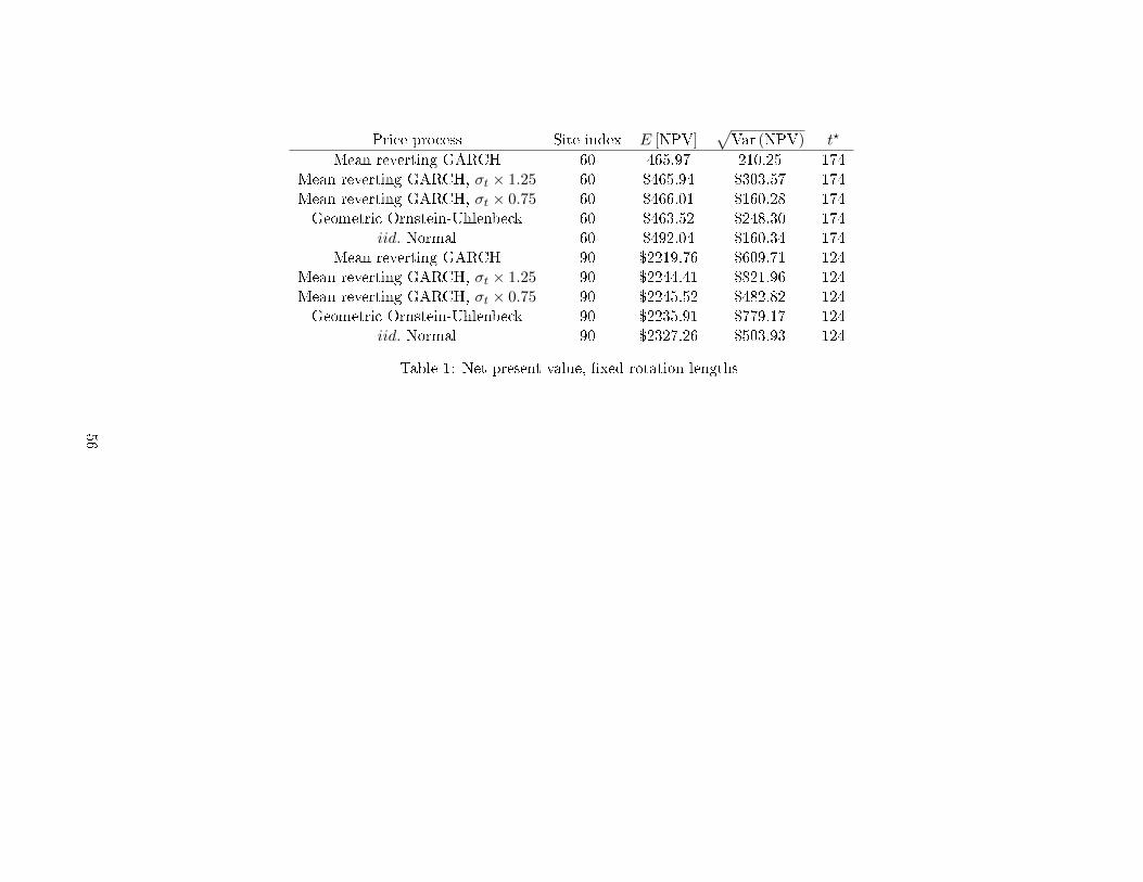
Price process Site index E [NPV]√Var (NPV) t?

Mean reverting GARCH 60 465.97 210.25 174Mean reverting GARCH, σt × 1.25 60 $465.94 $303.57 174Mean reverting GARCH, σt × 0.75 60 $466.01 $160.28 174Geometric Ornstein-Uhlenbeck 60 $463.52 $248.30 174

iid. Normal 60 $492.04 $160.34 174Mean reverting GARCH 90 $2219.76 $609.71 124

Mean reverting GARCH, σt × 1.25 90 $2244.41 $821.96 124Mean reverting GARCH, σt × 0.75 90 $2245.52 $482.82 124Geometric Ornstein-Uhlenbeck 90 $2235.91 $779.17 124

iid. Normal 90 $2327.26 $503.93 124

Table 1: Net present value, �xed rotation lengths

56

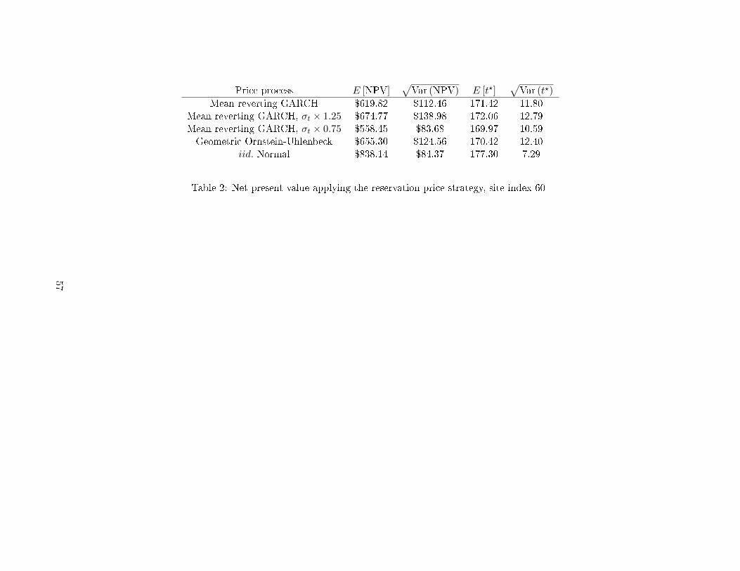
Price process E [NPV]√Var (NPV) E [t?]

√Var (t?)

Mean reverting GARCH $619.82 $112.46 171.42 11.80Mean reverting GARCH, σt × 1.25 $674.77 $138.98 172.06 12.79Mean reverting GARCH, σt × 0.75 $558.45 $83.68 169.97 10.59Geometric Ornstein-Uhlenbeck $655.30 $124.56 170.42 12.40

iid. Normal $838.14 $84.37 177.30 7.29

Table 2: Net present value applying the reservation price strategy, site index 60

57

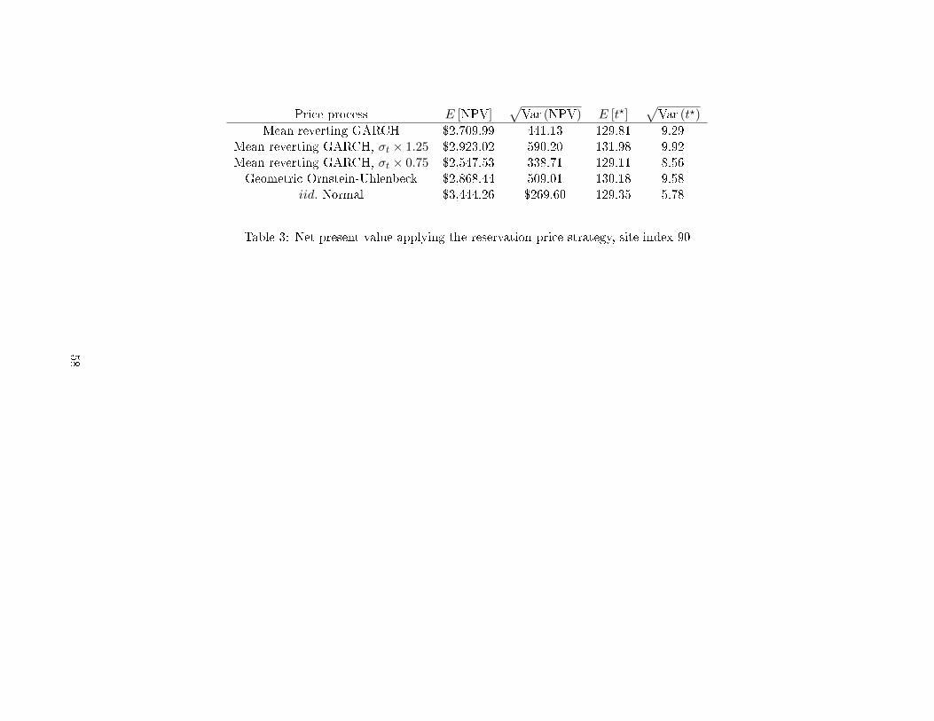
Price process E [NPV]√Var (NPV) E [t?]

√Var (t?)

Mean reverting GARCH $2,709.99 441.13 129.81 9.29Mean reverting GARCH, σt × 1.25 $2,923.02 590.20 131.98 9.92Mean reverting GARCH, σt × 0.75 $2,547.53 338.71 129.11 8.56Geometric Ornstein-Uhlenbeck $2,868.44 509.01 130.18 9.58

iid. Normal $3,444.26 $269.60 129.35 5.78

Table 3: Net present value applying the reservation price strategy, site index 90

58

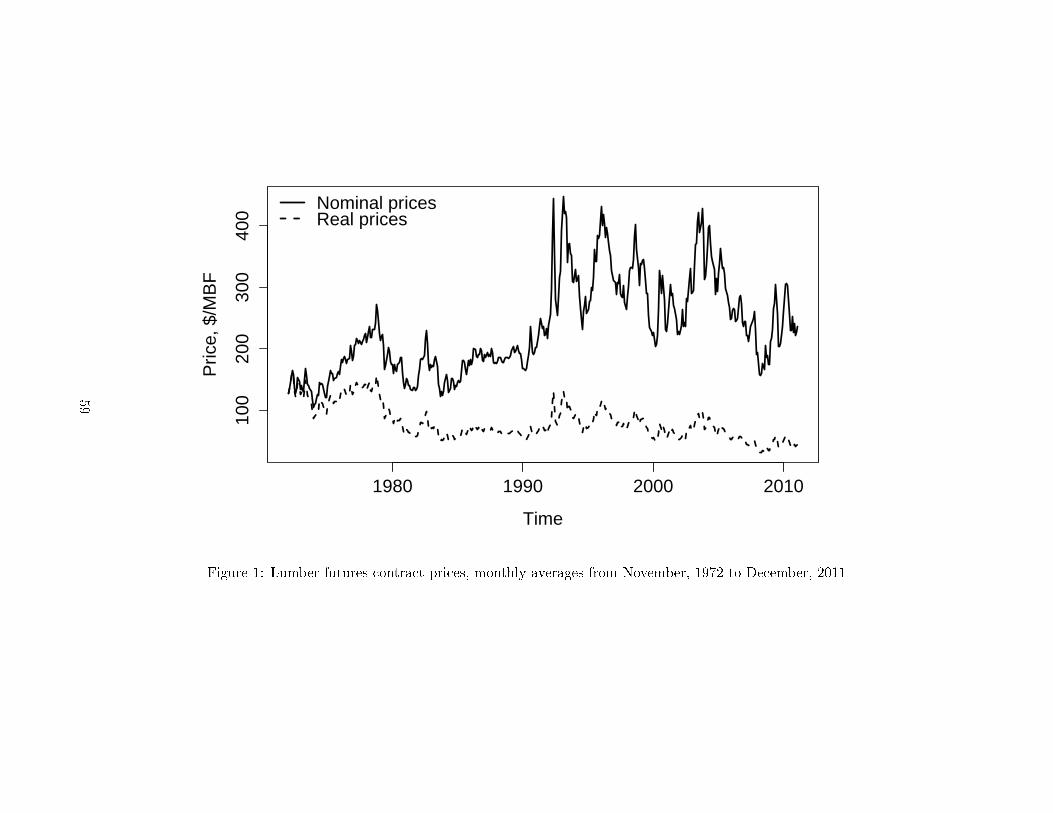
Time

Pric

e, $

/MB

F

1980 1990 2000 2010

100

200

300

400

Nominal pricesReal prices

Figure 1: Lumber futures contract prices, monthly averages from November, 1972 to December, 2011

59

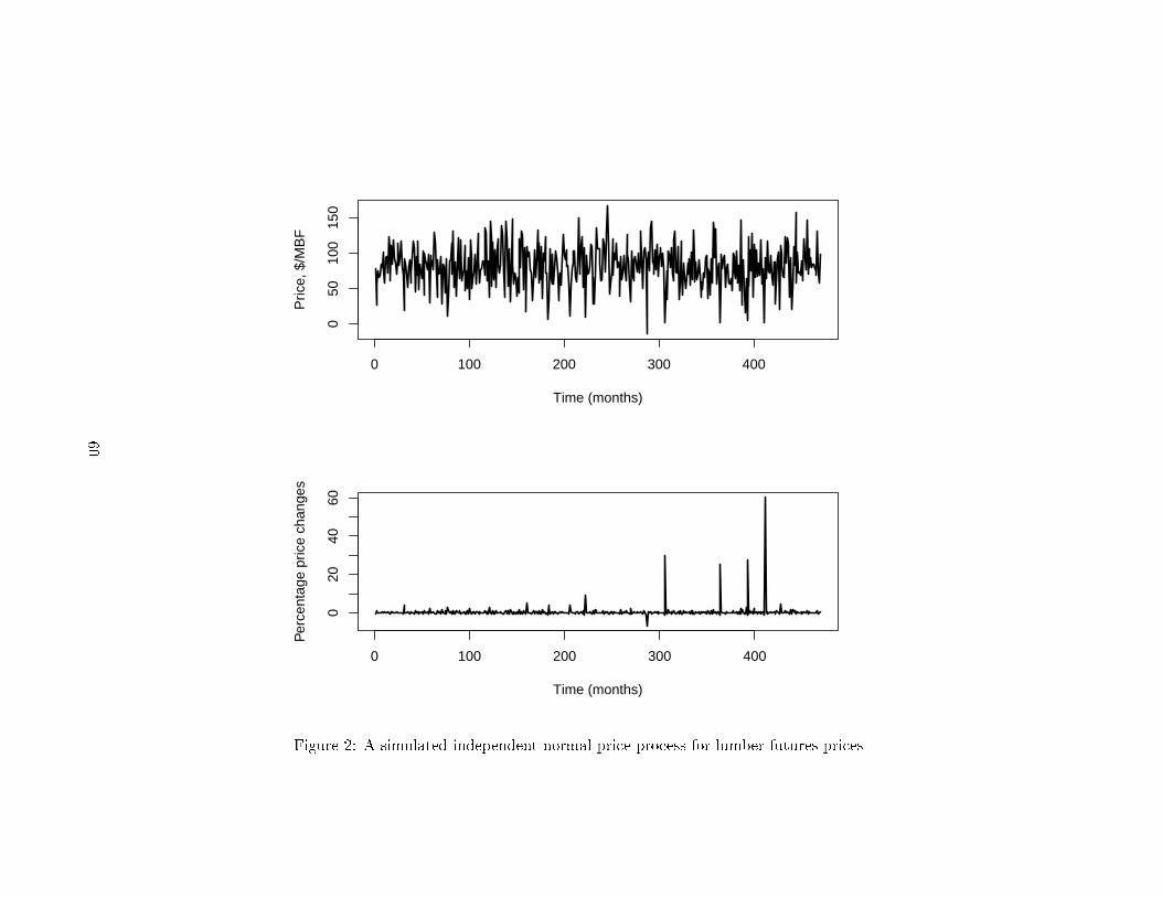
0 100 200 300 400

050

100

150

Time (months)

Pric

e, $

/MB

F

0 100 200 300 400

020

4060

Time (months)

Per

cent

age

pric

e ch

ange

s

Figure 2: A simulated independent normal price process for lumber futures prices

60

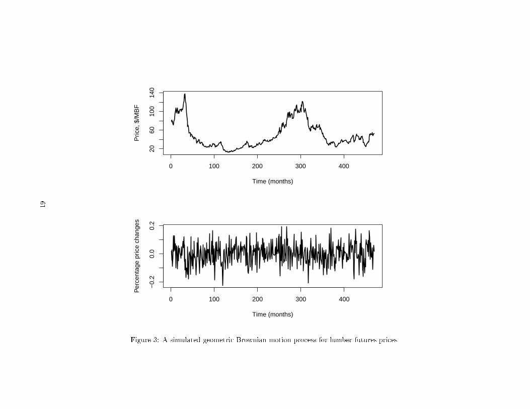
0 100 200 300 400

2060

100

140

Time (months)

Pric

e, $

/MB

F

0 100 200 300 400

−0.

20.

00.

2

Time (months)

Per

cent

age

pric

e ch

ange

s

Figure 3: A simulated geometric Brownian motion process for lumber futures prices

61

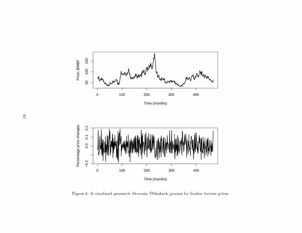
0 100 200 300 400

5010

015

0

Time (months)

Pric

e, $

/MB

F

0 100 200 300 400

−0.

20.

00.

10.

2

Time (months)

Per

cent

age

pric

e ch

ange

s

Figure 4: A simulated geometric Ornstein-Uhlenbeck process for lumber futures prices

62

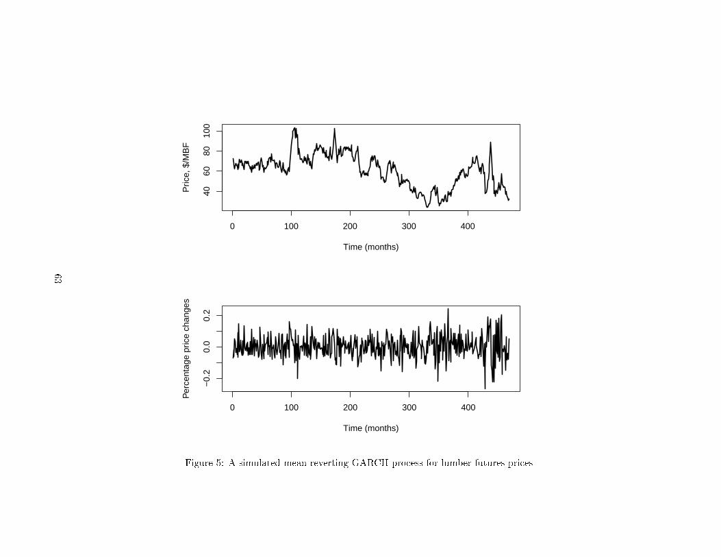
0 100 200 300 400

4060

8010

0

Time (months)

Pric

e, $

/MB

F

0 100 200 300 400

−0.

20.

00.

2

Time (months)

Per

cent

age

pric

e ch

ange

s

Figure 5: A simulated mean reverting GARCH process for lumber futures prices

63

●

●

●

●

●

●

●

●

●

●

●

●●

●

●

●

●

●●

●

●

●

●

●

●

●

●

●

●

●

●

●

●

●

●

●

●

●

●

●

●

●

●

●●

●

●

●

●

●

●

●

●

●

●

●●

●

●

●

●

●●

●

●

●

●

●●

●

●

●

●

●

●

●

●

●

●

●●

●

●

●●

●

●

●

●

●

●

●

●

●

●

●

●

●●

●

●●

●

●

●

●

●

●

●

●

●

●

●

●

●●●

●●

●

●

●

●

●

●

●

●

●

●

●●

●

●

●

●

●

●

●

●

●

●

●

●

●

●

●

●●

●●●

●

●

●

●

●

●

●

●●

●

●

●

●

●

●

●●

●●

●

●

●

●

●

●●

●

●

●

●

●●

●

●

●●

●

●●

●

●

●●

●

●

●

●

●

●

●

●

●

●

●

●

●

●

●

●

●

●

●

●

●●

●

●

●

●

●

●

●

●

●

●

●

●

●

●

●

●

●

●

●

●

●

●●

●

●

●

●

●●

●

●●

●

●

●

●

●

●●

●

●

●

●●

●

●

●

●

●

●

●

●

●

●

●

●

●

●●

●●

●

●

●

●

●

●

●

●

●

●

●

●

●

●●

●

●●

●

●

●

●

●

●●

●

●

●

●

●

●

●

●

●

●

●

●●

●

●●

●

●

●

●

●●

●

●

●

●

●

●

●

●●

●

●

●

●

●●

●●

●

●

●

●

●

●

●

●

●

●

●

●

●

●

●

●

●

●

●

●

●

●

●

●

●

●

●

●

●

●

●

●●

●

●

●

●

●

●

●

●

●

●

●

●

●

●

●

●

●

●

●

●●

●

●●

●

●

●

●

●

●

●

●

●

●

●

●

●

●

●

●

●

●

●

●●

●

●

●

●

●

●

●

●

●

●

●

●

●

●

●

●

●

●

●

●

●

●

●

●

●

●

●

●

●

●

●

●

●

●

●

●

●

●

●●

●

●

●

●

●

●

●

●

●

●

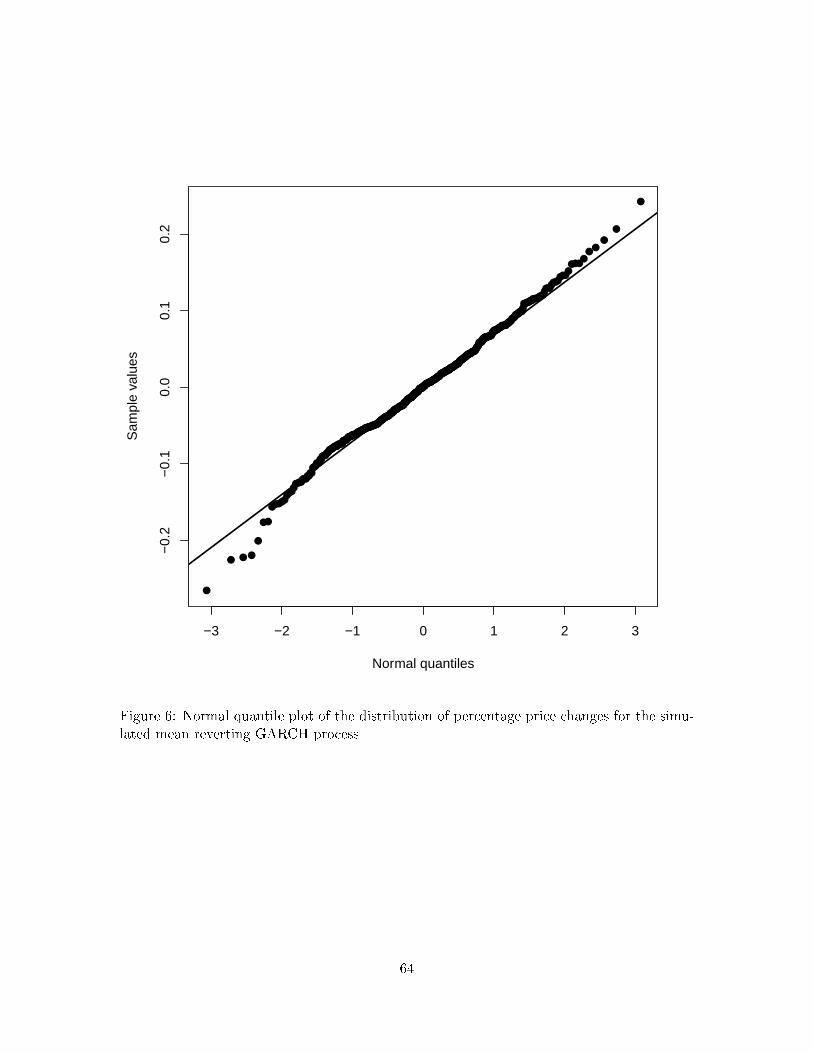
−3 −2 −1 0 1 2 3

−0.

2−

0.1

0.0

0.1

0.2

Normal quantiles

Sam

ple

valu

es

Figure 6: Normal quantile plot of the distribution of percentage price changes for the simu-lated mean reverting GARCH process

64

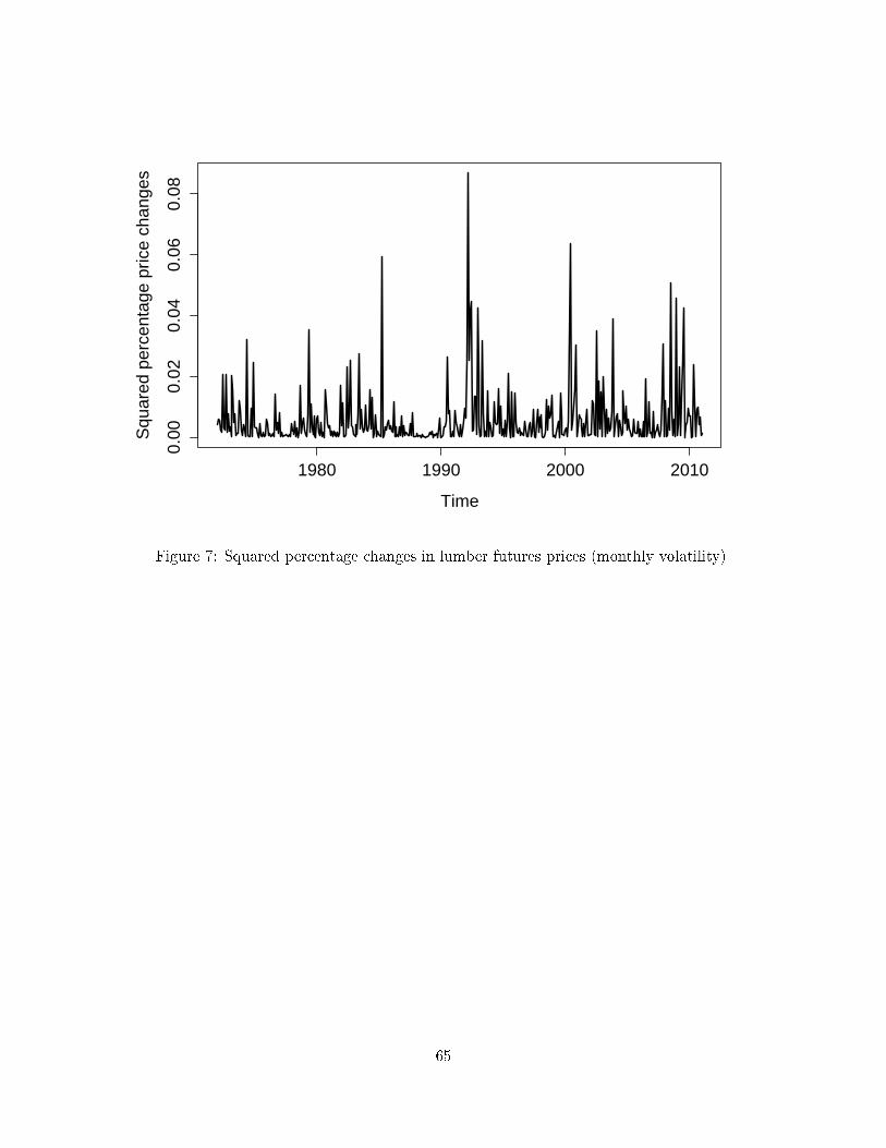
Time

Squ

ared

per

cent

age

pric

e ch

ange

s

1980 1990 2000 2010

0.00

0.02

0.04

0.06

0.08

Figure 7: Squared percentage changes in lumber futures prices (monthly volatility)

65

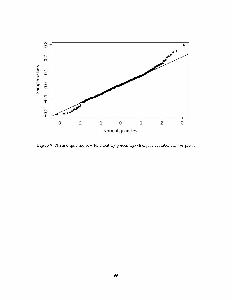
−3 −2 −1 0 1 2 3

−0.

2−

0.1

0.0

0.1

0.2

0.3

Normal quantiles

Sam

ple

valu

es

Figure 8: Normal quantile plot for monthly percentage changes in lumber futures prices

66

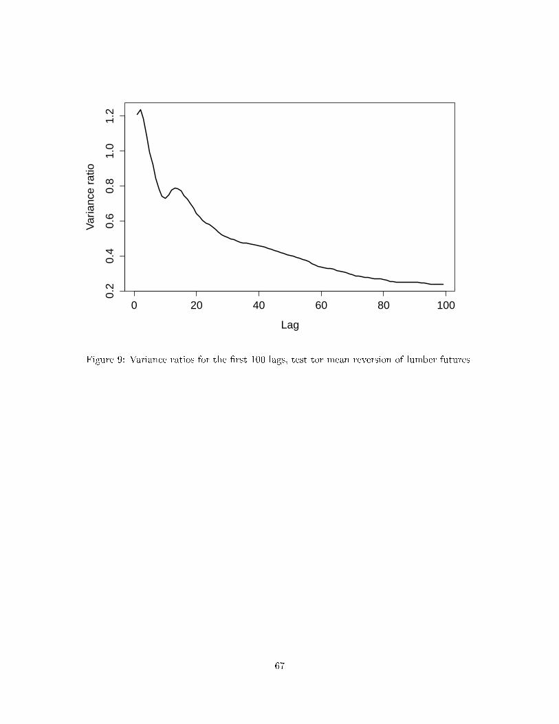
0 20 40 60 80 100

0.2

0.4

0.6

0.8

1.0

1.2

Lag

Var

ianc

e ra

tio

Figure 9: Variance ratios for the �rst 100 lags, test tor mean reversion of lumber futures

67

●●●●●●●●●●●●●●●●●●

●●

●

●

●

●

●

●

●

●

●

●

●

●

●

●

●

●

●

●●

●●

●●

●●

●●

●●

●●

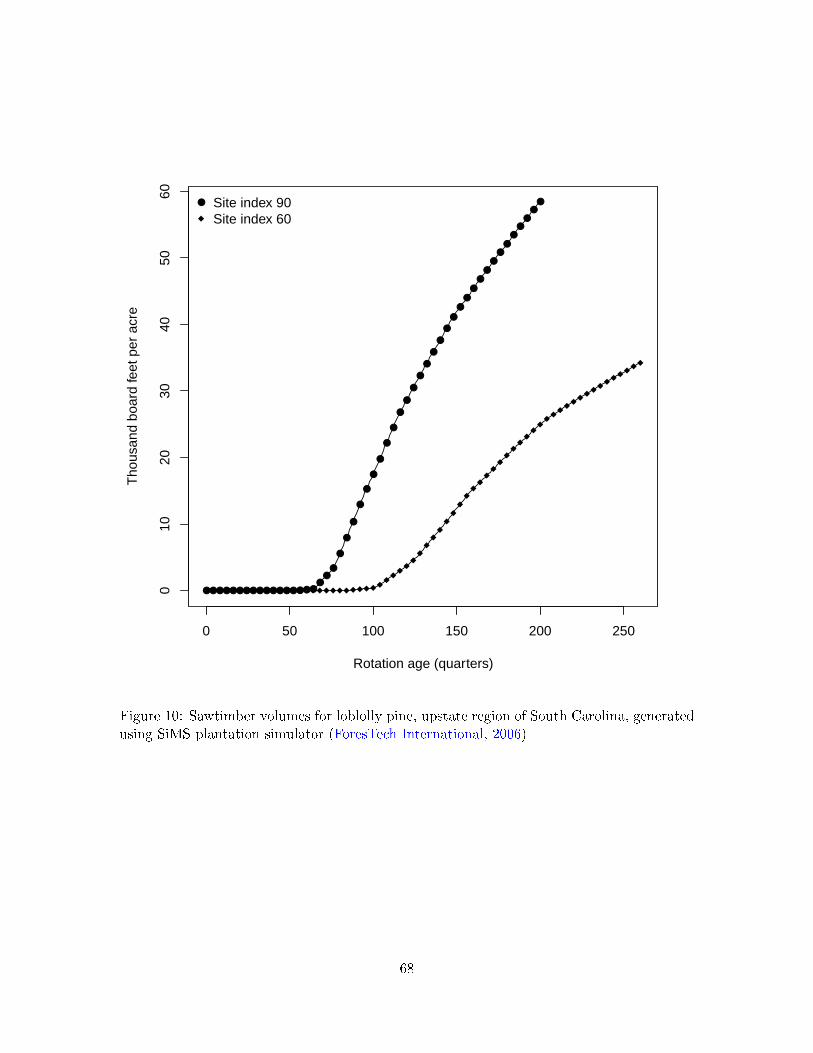
0 50 100 150 200 250

010

2030

4050

60

Rotation age (quarters)

Tho

usan

d bo

ard

feet

per

acr

e

● Site index 90Site index 60

Figure 10: Sawtimber volumes for loblolly pine, upstate region of South Carolina, generatedusing SiMS plantation simulator (ForesTech International, 2006)

68

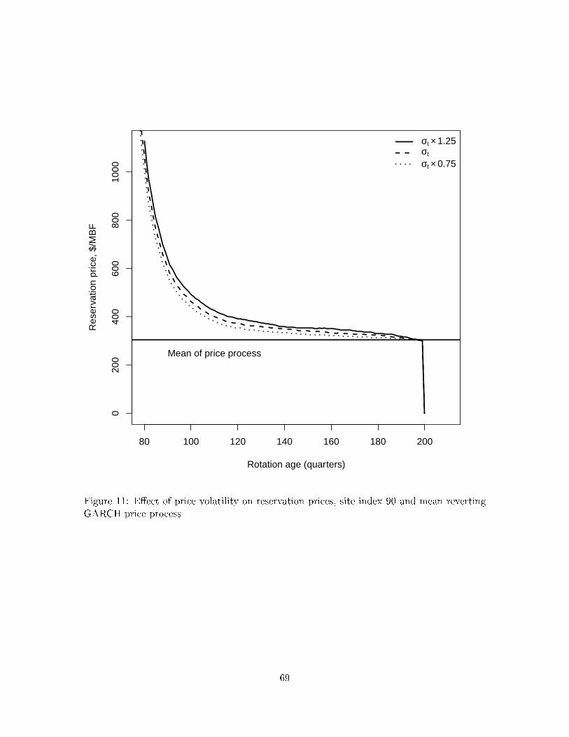
80 100 120 140 160 180 200

020

040

060

080

010

00

Rotation age (quarters)

Res

erva

tion

pric

e, $

/MB

F

σt × 1.25σt

σt × 0.75

Mean of price process

Figure 11: E�ect of price volatility on reservation prices, site index 90 and mean revertingGARCH price process

69

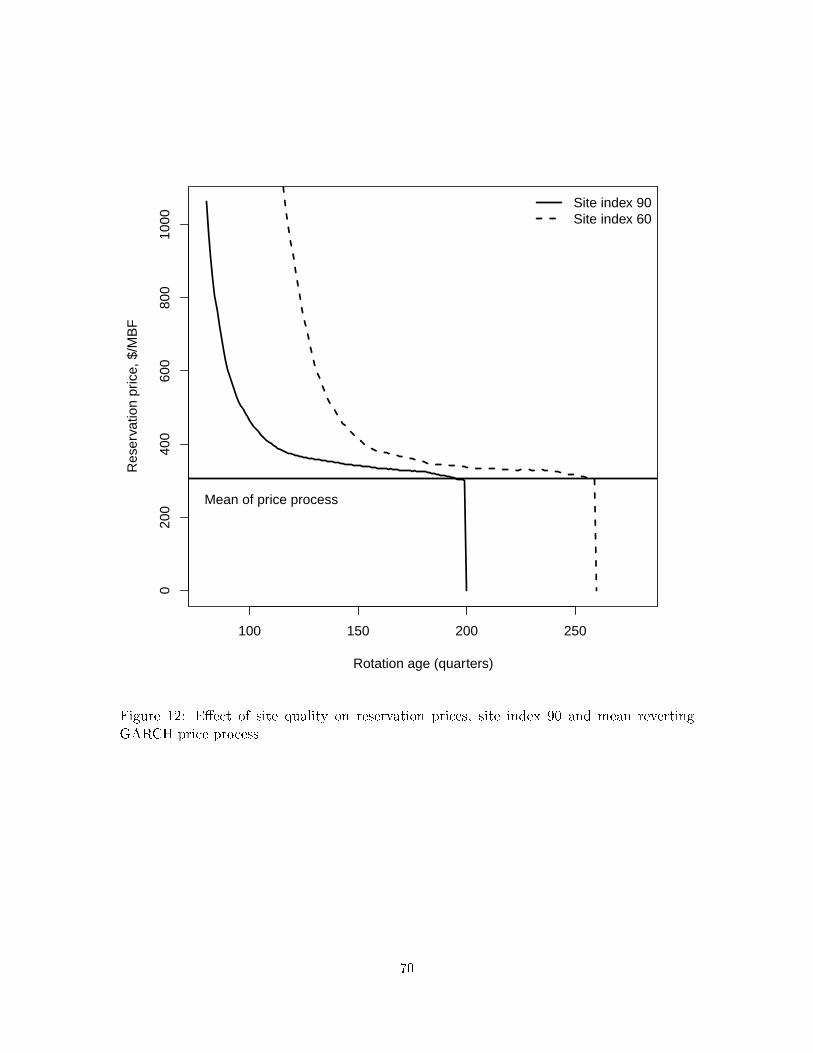
100 150 200 250

020

040

060

080

010

00

Rotation age (quarters)

Res

erva

tion

pric

e, $

/MB

F

Site index 90Site index 60

Mean of price process

Figure 12: E�ect of site quality on reservation prices, site index 90 and mean revertingGARCH price process

70

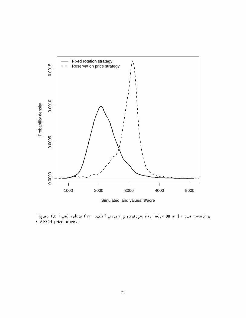
1000 2000 3000 4000 5000

0.00

000.

0005

0.00

100.

0015

Simulated land values, $/acre

Pro

babi

lity

dens

ity

Fixed rotation strategyReservation price strategy

Figure 13: Land values from each harvesting strategy, site index 90 and mean revertingGARCH price process

71

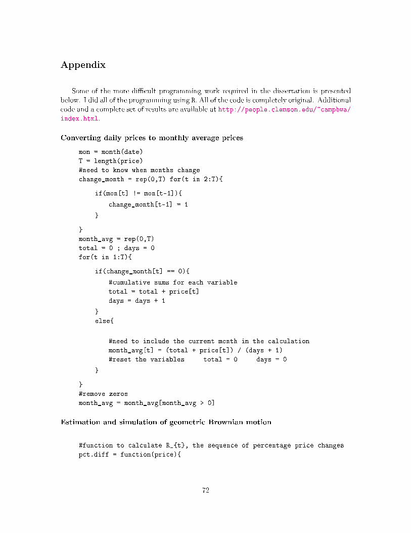
Appendix

Some of the more di�cult programming work required in the dissertation is presentedbelow. I did all of the programming using R. All of the code is completely original. Additionalcode and a complete set of results are available at http://people.clemson.edu/~campbwa/index.html.

Converting daily prices to monthly average prices

mon = month(date)

T = length(price)

#need to know when months change

change_month = rep(0,T) for(t in 2:T){

if(mon[t] != mon[t-1]){

change_month[t-1] = 1

}

}

month_avg = rep(0,T)

total = 0 ; days = 0

for(t in 1:T){

if(change_month[t] == 0){

#cumulative sums for each variable

total = total + price[t]

days = days + 1

}

else{

#need to include the current month in the calculation

month_avg[t] = (total + price[t]) / (days + 1)

#reset the variables total = 0 days = 0

}

}

#remove zeros

month_avg = month_avg[month_avg > 0]

Estimation and simulation of geometric Brownian motion

#function to calculate R_{t}, the sequence of percentage price changes

pct.diff = function(price){

72

PCT = rep(0,length(price))

d = diff(price)

for(t in 1:length(price)){

PCT[t] = d[t] / price[t]

}

PCT = PCT[-length(PCT)]

return(PCT)

}

#percentage price changes

R = pct.diff(price)

#estimation of the drift parameter

mean(R)

#estimate of the variance parameter

sd(R)

#Simulation of the price series

GBM.sim <- function(P_0 = 80, length = 2000, mu = 0.002461,

sigma = 0.09592){

P = rep(P_0, length)

epsilon = rnorm(length) #standard normal

for(i in 2:length){

P[i] = P[i-1] * (1 + mu) + sigma * P[i - 1] * epsilon[i]

}

return(P)

}

Estimation and simulation of the geometric Ornstein-Uhlenbeck process

R = pct.diff(price)

Z = 1/price[-470]

#regression equation to find the parametervalues

summary(lm(R ~ Z))

OU.sim = function(length = 2000, mu = 80.0356, eta = 0.03721,

sigma = 0.09557){

P_0 = mu #starting price is the mean

P = rep(P_0,length)

for(i in 2:length){

P[i] = P[i-1] + eta * (mu - P[i-1]) + sigma * rnorm(1) * P[i-1]

}

return(P)

}

73

Estimation and simulation of a geometric Ornstein-Uhlenbeck process with GARCH

price changes

require(fGARCH)

garch.model = garch(pct.diff(price))

#this provides the GARCH parameters

summary(garch.model)

GARCH.sim = function(mu = 80.0356, eta = 0.03721, omega = 0.000294,

alpha = 0.0949, beta = 0.855, length = 1000){

specs = garchSpec(model = list(omega = omega, alpha = alpha,

beta = beta))

sigma = garchSim(spec = specs, n = length)

P_0 = mu #starting price, known

P = rep(P_0,length)

for(i in 2:length){

P[i] = P[i-1] + eta * (mu - P[i-1]) + sigma[i] * P[i-1]

}

return(P)

}

Calculation of the expected value of a truncated normal distribution

#mu is the mean, stdev is the standard deviation, and

#a is the point of truncation:

#E[x|x>a], the function assumes positive truncation

e.normal = function(x, mean = 427.0379, stdev = 31.28014){

value = x * ((1 / (stdev * sqrt(2 * pi))) * exp((-0.5)

* ((x - mean) / stdev)^2))

return(value)

}

cond.exp.normal = function(mean = 427.0379, stdev = 31.28014, a = 0){

value = integrate(e.normal, a, Inf, mean = mean, stdev = stdev)$value

/ (1 - pnorm(a, mean = mean, sd = stdev))

return(value)

}

cond.exp.normal(a = 427.0379)

#the result is 451.9958

74

The discrete Faustmann model

#expected value of bare land with given parameter values:

faustmann = function(price = 150, r = 0.05, Cp = 250, vf = hq){

t = 1:500

beta = 1 / (1 + r/4)

t_star = which.max((beta^t * price * vf(t) - Cp)/(1 - beta^t))

NPV = (beta^t_star * price * vf(t_star) - Cp)/(1 - beta^t_star)

return(list(Optimal.rotation = t_star, NPV = NPV))

}

Backward recursion model for iid normal price process

mu = 427.0379; stdev = 151.72; r = 0.05

#monthly discount rate

beta = 1 / (1+(r/12))

#set the volume function to either hq or lq

vf = hq

#planting costs

Cp = 250

#initial estimate of the value of bare land

lambda = faustmann(price = mu, Cp = Cp, vf = vf)$NPV

#define the value function, call this function during the RP calculation

J = function(t, RP = 0){

value = (((1 - pnorm(RP, mean = mu, sd = stdev)) *

cond.exp.normal(a = RP, mean = mu, stdev = stdev) * vf(t)) +

(pnorm(RP, mean = mu, sd = stdev) * RP * vf(t))) + lambda

return(max(value, 0))

}

T = 800

RP = rep(0,T)

t = T - 1

while(t >= 1){

RP[t] = (beta * J(t + 1, RP[t + 1]) - lambda) / vf(t)

t = t - 1 #count backwards

}

Solving for reservation prices using Monte Carlo simulation, mean reverting

GARCH process

#Monte Carlo land value function

#the function assumes that harvesting decisions are made quarterly

75

#the function has two built-in volume functions: 1 for high quality plots

#and 2 for low quality plots

#prices is a vector of stumpage prices: timber price - harvest costs

land.value = function(initial.time = 1, ending.time = 200,

volume.function = "hq", r = 0.05, prices, res_price){

#discount factor

beta = 1 / (1 + r/4)

#determine the volume function and minimum and maximum harvest dates

if(volume.function == "hq"){

vf = hq

t_min = 100

t_max = 200

} else

if(volume.function == "lq"){

vf = lq

t_min = 30 * 4

t_max = 65 * 4

}

#the sequence of the control variable

harvest = rep(FALSE, ending.time)

#vector to store profits

profit = rep(0, ending.time)

current.time = initial.time

while(current.time <= ending.time && harvest[current.time] == FALSE){

#if timber is below the minimum age, there can be no harvest

if(current.time < t_min){

harvest[current.time] = FALSE

current.time = current.time + 1

}

#contract owner may choose to harvest or delay

else if(current.time >= t_min && current.time < t_max){

#don't harvest if current price is less than the current RP

if(prices[current.time] < res_price[current.time]){

harvest[current.time] = FALSE

current.time = current.time + 1

}

#otherwise, harvest

else{

harvest[current.time] = TRUE

profit[current.time] = prices[current.time] * vf(current.time)

76

* beta^(current.time - initial.time)

#store the value of the rotation length

rotation.length = current.time

}

}

#contract owner always harvests when the age of trees is t_max

else if(current.time == t_max){

harvest[current.time] = TRUE

profit[current.time] = prices[current.time] * vf(current.time)

* beta^(current.time - initial.time)

#store the value of the rotation length

rotation.length = current.time

}

}

return(list(Profits = sum(profit), Harvest.times = harvest, profit))

}

nsim = 5000 #number of simulations

N = 200 #number of periods in the model

prices = matrix(nrow = nsim, ncol = N)

for(i in 1:nsim){

prices[i,] = GARCH.sim(mu = mu, eta = eta, omega = omega,

alpha = alpha, beta = beta, length = N)

}

beta = 1 / (1 + (r / 4))

lambda = 1610.877 #337.4541 #set to Faustmann value

vf = hq

n = 0 #start at time N

value = rep(0, N)

RP = rep(0,N)

### Start the backward recursion algorithm ###

while((N - n) >= 250){

v = rep(0,nsim)

for(i in 1:nsim){

#the value for the ith simulated price

v[i] = land.value.MC(initial.time = N - n, ending.time = N,

volume.function = "hq", prices = prices[i,],

res_price = RP)$Profits

}

#the expected value function is

value[N-n] = mean(v) + lambda

77

#the reservation price at N-2 is

RP[N-n-1] = (beta * value[N-n] - lambda) / vf(N-n)

n = n + 1

}

Simulation model of the reservation price strategy

#Model inputs: price process, discount rate, volume function,

#and set of reservation prices.

#Model outputs: profits and rotation lengths from applying

#the reservation price strategy.

#duration is the length of the simulation, 1,000 quarters should be enough,

#anything beyond this will not affect discounted profits

#the function assumes that harvesting decisions are made quarterly

land.value = function(duration = 1000, volume.function = "hq", r = 0.05,

prices, res_price){

#discount factor

beta = 1 / (1 + r/4)

#set NA values of the reservation price to infinity

for(i in 1:length(res_price)){

if(is.na(res_price[i])){

res_price[i] = Inf

}

}

#store values for the volume function in the vector vf

vf = rep(0, duration)

if(volume.function == "hq"){

vf = hq

t_min = 25 * 4

t_max = 50 * 4

} else

if(volume.function == "lq"){

vf = lq

t_min = 30 * 4

t_max = 65 * 4

}

#check to make sure the length of the price vector

#matches the duration of the contract (in months)

if(length(prices) != duration){

print("Length of the price vector needs to match the duration")

stop()

78

}

#the sequence of the control variable

harvest = rep(FALSE, duration)

rotation.time = 0

#starts with planting

total.time = 1

#an object to store all of the rotation lengths

rotation.lengths = 0

#vector to store profits

profit = rep(0, duration)

while(total.time < duration){

#needs to be incremented here

rotation.time = rotation.time + 1

total.time = total.time + 1

#if timber is below the minimum age, there can be no harvest

if(rotation.time < t_min){

harvest[total.time] = FALSE

}

#contract owner may choose to harvest or delay

else if(rotation.time >= t_min && rotation.time < t_max){

#don't harvest if current price is less than the current RP

if(prices[total.time] < res_price[rotation.time]){

harvest[total.time] = FALSE

}

#otherwise, harvest

else{

harvest[total.time] = TRUE

profit[total.time] = prices[total.time] * vf(rotation.time) *

beta^total.time

#store the value of the rotation length

rotation.lengths = c(rotation.lengths, rotation.time)

#reset the time for each rotation

rotation.time = 0

}

}

#contract owner always harvests when the age of trees is t_max

else if(rotation.time == t_max){

harvest[total.time] = TRUE

profit[total.time] = prices[total.time] * vf(rotation.time) *

beta^total.time

#store the value of the rotation length

79

rotation.lengths = c(rotation.lengths, rotation.time)

#reset the time for each rotation

rotation.time = 0

}

}

return(list(Profits = sum(profit), Harvest.times = harvest,

Rotation.lengths = rotation.lengths[-1], profit))

}

Simulation model for the valuation of bare land with constant rotation lengths

r = 0.05

beta = 1 / (1 + (r/4))

#number of simulations

nsim = 10000

profit = rep(0, nsim)

t_star = faustmann(price = 317.8848, r = 0.05, Cp = 250,

vf = lq)$Optimal.rotation

#ten rotations

time = seq(from = t_star, to = t_star*10, by = t_star)

#create a matrix of prices

price = matrix(0, nrow = nsim, ncol = t_star * 10)

for(i in 1:nsim){

price[i,] = GARCH.sim(length = t_star * 10)

}

#low quality site

for(i in 1:nsim){

for(t in time){

profit[i] = sum(beta^time * price[i, time] * lq(t_star))

}

}

lq_profit = profit

#high quality site

t_star = faustmann(price = 317.8848, r = 0.05, Cp = 250,

vf = hq)$Optimal.rotation

time = seq(from = t_star, to = t_star*10, by = t_star)

for(i in 1:nsim){

for(t in time){

80

profit[i] = sum(beta^time * price[i, time] * hq(t_star))

}

}

hq_profit = profit

81