using model life tables to assess the plausibility of directly-constructed historical life tables
TRANSCRIPT
125
Using Model Life Tables to Assess the Plausibility of Directly-
Constructed Historical Life Tables
Sulaiman Bah, Prof
College of Applied Medical Sciences
University of Dammam (formally King Faisal University)
Dammam
Saudi Arabia
Email: [email protected]
ABSTRACT
This paper focuses on the historical life tables that were directly constructed, independent of
model life tables. For such life tables, the standard model life tables of Coale and Demeny and
those of United Nations can be used in assessing their quality. The paper deals with one aspect of
the quality of such life tables, namely, the extent to which the underlying mortality level is correctly
estimated. A method is developed to detect the presence of under-estimation of the underlying
mortality level. The method is used in conjunction with the output from the COMPAR program in
the United Nations MORTPAK software. The method is applied to South African life tables for
white males and females from 1921 to 1985. The key finding is that there was remarkable
underestimation of mortality in the South African published life tables for both white males and
females for the period 1921 to 1985.
Key words
Model life table, historical life table, South Africa, mortality, MORTPAK
1. Introduction
The development of model life tables has a long history dating back to the 1950s. Their uses
in demography are quite vast, especially in the sub-specialty of indirect techniques for demographic
estimation (United Nations, 1983). This paper is concerned with one specific use, that of assessing
the plausibility of a life table that was directly constructed, independent of model life tables. The
reference model life tables used for the study are nine in all, four patterns of the Coale-Demeny
(also called families) and five patterns of the United Nations (Coale and Demeny, 1966; United
Nations, 1982). The study life tables of interest are those in the recent historical period, the 1980s
and earlier, not the contemporary period of the 2000s. Because of the epidemiologic transition that
different countries are undergoing, the aforementioned model life tables are arguably more
applicable to the recent historical period than the contemporary one. For the contemporary period,
several alternative life table systems have been developed to cater for different epidemiological
regimes. These include; a) the modified Coale-Demeny life tables that cater for population at very
low levels of mortality (Coale and Guo, 1989), b) the INDEPTH model life table that caters for
African countries with relatively high mortality and high rates of infectious diseases (INDEPTH
Network, 2004), and, c) the WHO model life tables that cater for the relationship between
childhood mortality and adult mortality (Murray et al, 2003).
126
The study of historical life tables is important for several reasons like, if the historical life
tables have been used in other applications, their assessment is of relevance for all those
applications; if data are needed for mortality projections, the assessment of the historical part of the
time series data would be an important component of that projection exercise; related to afore-
mentioned point, if time series in life tables are needed for population projections, then, again, the
assessment of the historical life tables is of relevance.
The next section identifies some specific issues involved in the assessment of historical life
tables. It outlines a theoretical exposition of the problem and shows the gap that exists in addressing
the problem at hand. This is followed by the introduction of a new method to solve the problem
identified. The method is applied to South African historical life tables data and the results are
presented in the Application section. The discussion of the results and the conclusion are presented
in the last section.
2. Theoretical exposition
A standard approach for assessing the similarity between a given life table and a series of
model life tables is to compute a measure of dissimilarity, δ, based on one of the life table
parameters. The basic premise in this theoretical exposition is that this same measure of
dissimilarity, δ, can be used as a measure of quality of the study life table. If δ has the property for a
perfect fit, δ=0 and δ increases in magnitude as the two life tables become disimilar, then the trend
in δ values also attest to the quality of the series of study life tables. If, for example, the values of δ
fluctuate rapidly when in reality there was no genuine fluctuation in mortality, then this calls to
question the quality of the series of study life tables. Similarly, if δ is found to be out of the normal
expected range, then the quality of the study life tables should also be called to question.
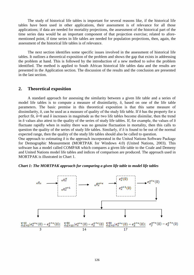
One approach to estimating δ is the approach incorporated in the United Nations Software Package
for Demographic Measurement (MORTPAK for Windows 4.0) (United Nations, 2003). This
software has a model called COMPAR which compares a given life table to the Coale and Demeny
and United Nations model life tables and indices of comparison are produced. The approach used in
MORTPAK is illustrated in Chart 1.
Chart 1: The MORTPAK approach for comparing a given life table to model life tables
127
The MORTPAK approach proceeds as follows: for each age group, the value of a study
life table is compared with model life table. When a pair of model values (at two successive
levels, α and α+1) are found to bracket the study life table value, they are used to calculate the
interpolation factor, such that, 0<ε <1. After the interpolation factor has been obtained, it is
used to interpolate between two model life expectancies at birth, and at levels α and
α+1 respectively, to obtain the ‘implied life expectancy at birth’, . From these implied life
expectancies at birth, four indices are derived: 1) For the ages below 10 years (3 age groups), the
average of the absolute deviations between the implied life expectancies at birth and the median of
the implied life expectancies at birth (AD1 for short). 2) For the ages above 10 years (14 age
groups), the average of the absolute deviations between the implied life expectancies at birth and
the median of the implied life expectancies at birth (AD2). 3) For all the ages (17 age groups), the
average of the absolute deviations between the implied life expectancies at birth and the median of
the implied life expectancies at birth (AD3). 4) The difference between the median implied life
expectancies at birth for ages 0–10 and the median implied life expectancies at birth for ages above
10 years old (AD4). For AD1, AD2 and AD3, the minimum is zero while there is no fixed
maximum. The lower the values the better the fit and a value of zero shows perfect fit. For AD4,
values could be positive or negative, and again, the lower the (absolute) values the better and
similarly, a value of zero shows perfect fit.
When the quality of life tables are good, this MORTPAK approach is very insightful in
identifying the model life table that best suits the study. With a time series of study life tables, the
MORTPAK approach allows a mapping of the underlying epidemiologic transition using model life
tables. This approach was used in historical study of high quality life tables from Mauritius (Bah
and Teklu, 1992). The aim of this study is to address the converse of this problem. The study further
aims to address the following questions: ‘is the level of mortality underestimated relative to a model
life table?’, ‘If there is underestimation of mortality, how serious is it?’. The study is not addressing
the question of the degree of completeness of death registration. In order to answer the questions
posed, we need information on the extremes (minimum and maximum) and we need to relate the
life expectancy at birth in the observed life table with the implied life expectancy at birth in the
model life table. The literature review did not discover any method addressing these questions. As
such, a new method that uses only the outputs from MORTPAK was proposed.
3. The proposed method
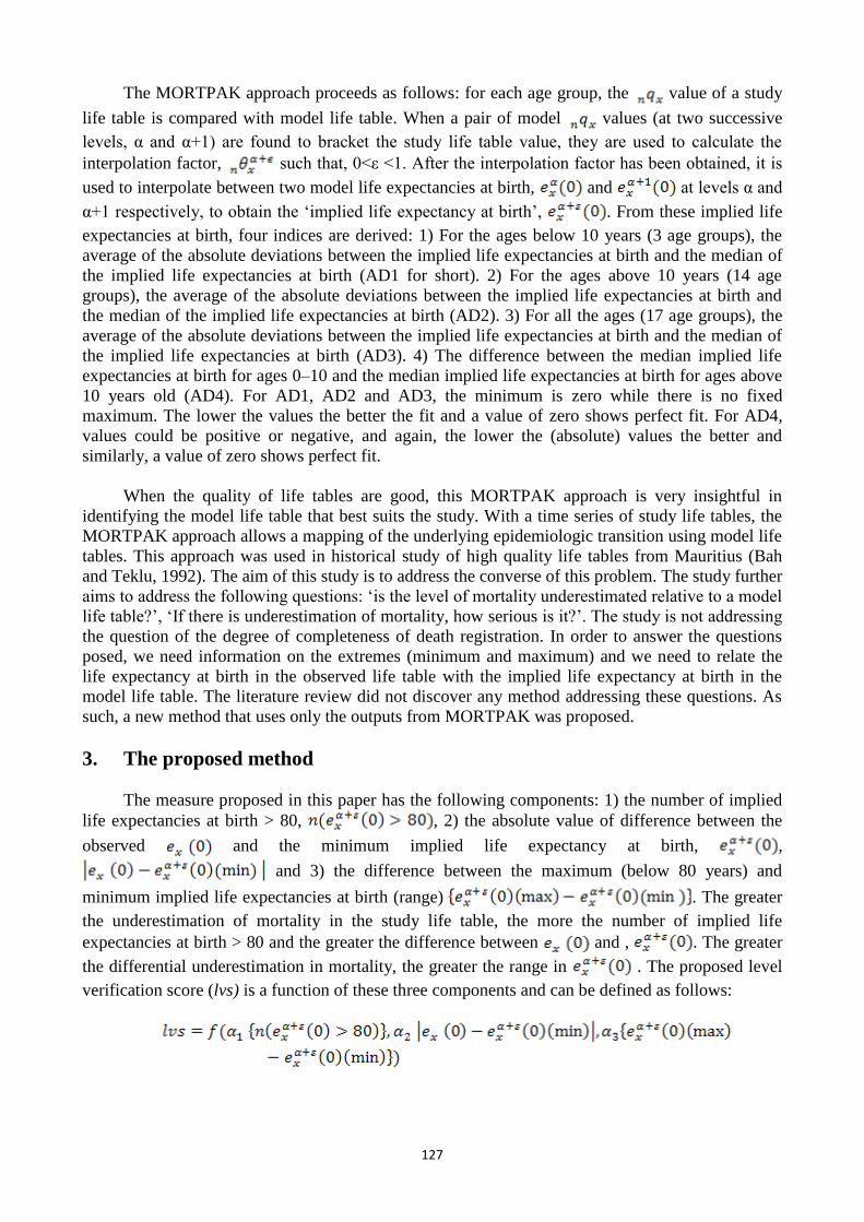
The measure proposed in this paper has the following components: 1) the number of implied
life expectancies at birth > 80, , 2) the absolute value of difference between the
observed and the minimum implied life expectancy at birth, ,
and 3) the difference between the maximum (below 80 years) and
minimum implied life expectancies at birth (range) . The greater
the underestimation of mortality in the study life table, the more the number of implied life
expectancies at birth > 80 and the greater the difference between and , . The greater
the differential underestimation in mortality, the greater the range in . The proposed level
verification score (lvs) is a function of these three components and can be defined as follows:
128
The challenge at hand is to specify the form of the function and to identify the values of the
constants, , and . This is not the case in which there are values for the outcome variable, lvs,
and for each of the independent variables. Had it been so, some form of regression model could
have been fitted to the data and the values of , and be determined. What we have is the
situation in which, for all the age groups, one life table function is fitted to the same model life table
and an implied life expectancy at birth is derived. In some cases there would be no implied life
expectancies at birth that are greater than 80 years. In other cases, for some ages, the implied life
expectancy at birth could be greater than 80 years (implying underestimation of mortality) while for
others, it would be less than 80 years. The difference between the observed life expectancy at birth
and the implied ones could be any number, for example, 0, 1, 2,5, or 2,8. The difference between
the maximum and minimum implied life expectancy at birth again could be any number, for
example, 2, 5 or 10. It is virtually impractical to try to predict the different possible outcomes.
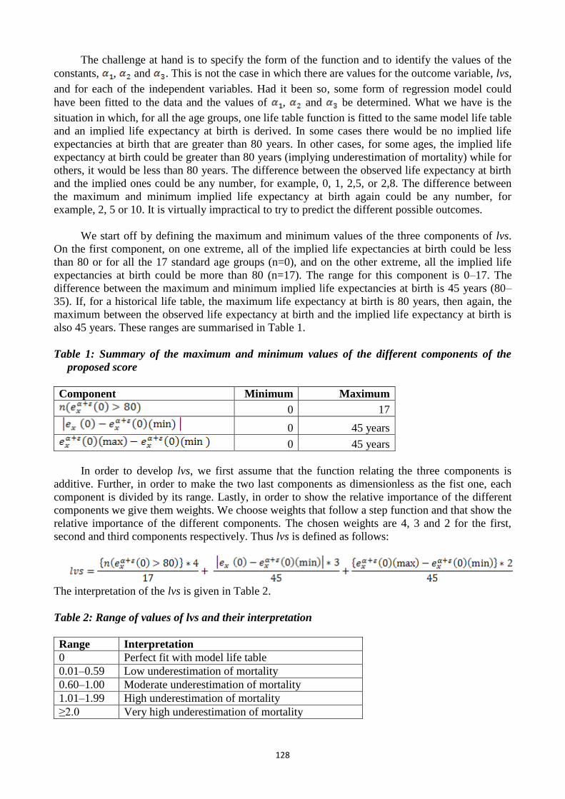
We start off by defining the maximum and minimum values of the three components of lvs.
On the first component, on one extreme, all of the implied life expectancies at birth could be less
than 80 or for all the 17 standard age groups (n=0), and on the other extreme, all the implied life
expectancies at birth could be more than 80 (n=17). The range for this component is 0–17. The
difference between the maximum and minimum implied life expectancies at birth is 45 years (80–
35). If, for a historical life table, the maximum life expectancy at birth is 80 years, then again, the
maximum between the observed life expectancy at birth and the implied life expectancy at birth is
also 45 years. These ranges are summarised in Table 1.
Table 1: Summary of the maximum and minimum values of the different components of the
proposed score
Component Minimum Maximum
0 17
0 45 years
0 45 years
In order to develop lvs, we first assume that the function relating the three components is
additive. Further, in order to make the two last components as dimensionless as the fist one, each
component is divided by its range. Lastly, in order to show the relative importance of the different
components we give them weights. We choose weights that follow a step function and that show the
relative importance of the different components. The chosen weights are 4, 3 and 2 for the first,
second and third components respectively. Thus lvs is defined as follows:
The interpretation of the lvs is given in Table 2.
Table 2: Range of values of lvs and their interpretation
Range Interpretation
0 Perfect fit with model life table
0.01–0.59 Low underestimation of mortality
0.60–1.00 Moderate underestimation of mortality
1.01–1.99 High underestimation of mortality
≥2.0 Very high underestimation of mortality
129
4. Application
The proposed method is applied to South African life tables for white males and females,
1921–1985. The published life tables were compared to the nine model life tables using the
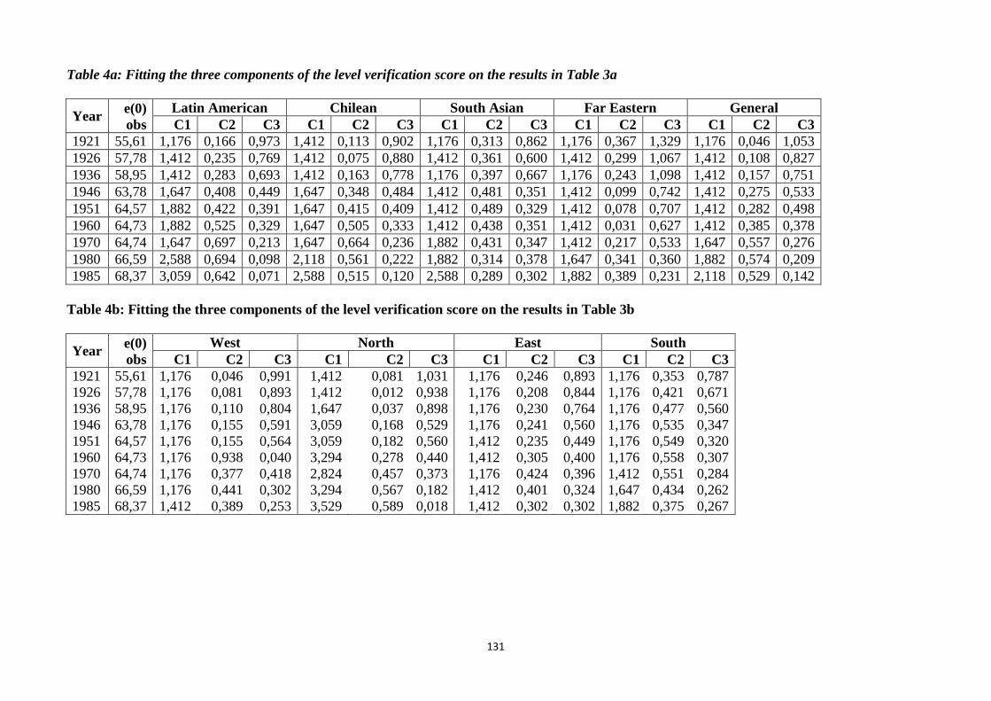
COMPAR program in MORTPAK. For males, the relevant information was extracted from the
results and are shown in Tables 3a and 3b. From these results, the first component (C1), second
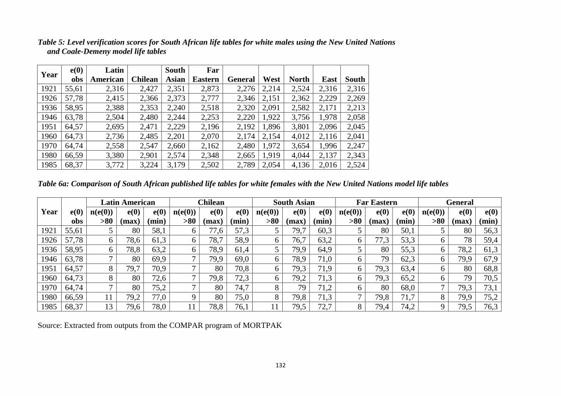
(C2) and third components (C3) were calculated and are shown in Tables 4a and 4b. The final
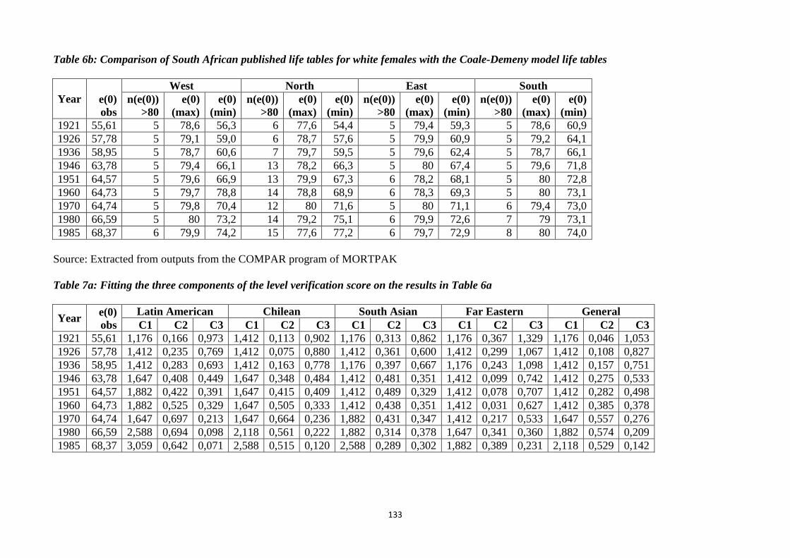
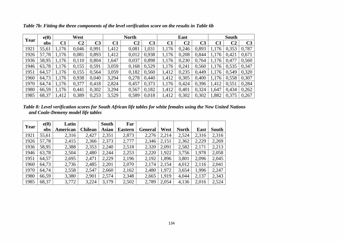
results for lvs are given in Table 5. For females, the corresponding results are shown in Table 6a
through to Table 8.
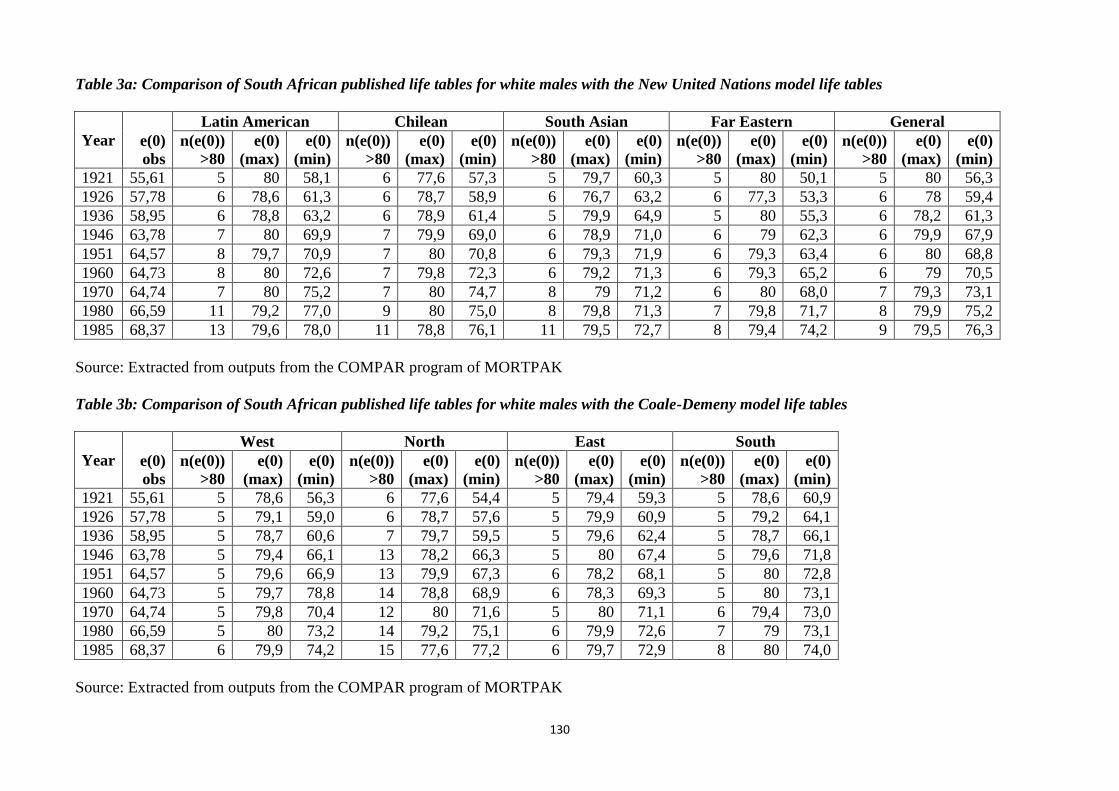
A cursory look at Tables 3a and 3b shows that there are problems with these life tables. For
each of the years, from 1921 to 1985, the fit to all the model life tables results in having some of the
implied life expectancy at birth being more than 80 years, with the numbers generally increasing
over time. The worst fit is for the North model in which, by 1985, 15 out of the 17 implied life
expectancies at birth were greater than 80 years. The lvs values in Table 3 are mostly over 2,0,
implying very high underestimation of mortality. To a very large extent these observations also hold
true for females.
130
Table 3a: Comparison of South African published life tables for white males with the New United Nations model life tables
Year e(0)
obs
Latin American Chilean South Asian Far Eastern General
n(e(0))
>80
e(0)
(max)
e(0)
(min)
n(e(0))
>80
e(0)
(max)
e(0)
(min)
n(e(0))
>80
e(0)
(max)
e(0)
(min)
n(e(0))
>80
e(0)
(max)
e(0)
(min)
n(e(0))
>80
e(0)
(max)
e(0)
(min)
1921 55,61 5 80 58,1 6 77,6 57,3 5 79,7 60,3 5 80 50,1 5 80 56,3
1926 57,78 6 78,6 61,3 6 78,7 58,9 6 76,7 63,2 6 77,3 53,3 6 78 59,4
1936 58,95 6 78,8 63,2 6 78,9 61,4 5 79,9 64,9 5 80 55,3 6 78,2 61,3
1946 63,78 7 80 69,9 7 79,9 69,0 6 78,9 71,0 6 79 62,3 6 79,9 67,9
1951 64,57 8 79,7 70,9 7 80 70,8 6 79,3 71,9 6 79,3 63,4 6 80 68,8
1960 64,73 8 80 72,6 7 79,8 72,3 6 79,2 71,3 6 79,3 65,2 6 79 70,5
1970 64,74 7 80 75,2 7 80 74,7 8 79 71,2 6 80 68,0 7 79,3 73,1
1980 66,59 11 79,2 77,0 9 80 75,0 8 79,8 71,3 7 79,8 71,7 8 79,9 75,2
1985 68,37 13 79,6 78,0 11 78,8 76,1 11 79,5 72,7 8 79,4 74,2 9 79,5 76,3
Source: Extracted from outputs from the COMPAR program of MORTPAK
Table 3b: Comparison of South African published life tables for white males with the Coale-Demeny model life tables
Year
e(0)
obs
West North East South
n(e(0))
>80
e(0)
(max)
e(0)
(min)
n(e(0))
>80
e(0)
(max)
e(0)
(min)
n(e(0))
>80
e(0)
(max)
e(0)
(min)
n(e(0))
>80
e(0)
(max)
e(0)
(min)
1921 55,61 5 78,6 56,3 6 77,6 54,4 5 79,4 59,3 5 78,6 60,9
1926 57,78 5 79,1 59,0 6 78,7 57,6 5 79,9 60,9 5 79,2 64,1
1936 58,95 5 78,7 60,6 7 79,7 59,5 5 79,6 62,4 5 78,7 66,1
1946 63,78 5 79,4 66,1 13 78,2 66,3 5 80 67,4 5 79,6 71,8
1951 64,57 5 79,6 66,9 13 79,9 67,3 6 78,2 68,1 5 80 72,8
1960 64,73 5 79,7 78,8 14 78,8 68,9 6 78,3 69,3 5 80 73,1
1970 64,74 5 79,8 70,4 12 80 71,6 5 80 71,1 6 79,4 73,0
1980 66,59 5 80 73,2 14 79,2 75,1 6 79,9 72,6 7 79 73,1
1985 68,37 6 79,9 74,2 15 77,6 77,2 6 79,7 72,9 8 80 74,0
Source: Extracted from outputs from the COMPAR program of MORTPAK
131
Table 4a: Fitting the three components of the level verification score on the results in Table 3a
Year e(0)
obs
Latin American Chilean South Asian Far Eastern General
C1 C2 C3 C1 C2 C3 C1 C2 C3 C1 C2 C3 C1 C2 C3
1921 55,61 1,176 0,166 0,973 1,412 0,113 0,902 1,176 0,313 0,862 1,176 0,367 1,329 1,176 0,046 1,053
1926 57,78 1,412 0,235 0,769 1,412 0,075 0,880 1,412 0,361 0,600 1,412 0,299 1,067 1,412 0,108 0,827
1936 58,95 1,412 0,283 0,693 1,412 0,163 0,778 1,176 0,397 0,667 1,176 0,243 1,098 1,412 0,157 0,751
1946 63,78 1,647 0,408 0,449 1,647 0,348 0,484 1,412 0,481 0,351 1,412 0,099 0,742 1,412 0,275 0,533
1951 64,57 1,882 0,422 0,391 1,647 0,415 0,409 1,412 0,489 0,329 1,412 0,078 0,707 1,412 0,282 0,498
1960 64,73 1,882 0,525 0,329 1,647 0,505 0,333 1,412 0,438 0,351 1,412 0,031 0,627 1,412 0,385 0,378
1970 64,74 1,647 0,697 0,213 1,647 0,664 0,236 1,882 0,431 0,347 1,412 0,217 0,533 1,647 0,557 0,276
1980 66,59 2,588 0,694 0,098 2,118 0,561 0,222 1,882 0,314 0,378 1,647 0,341 0,360 1,882 0,574 0,209
1985 68,37 3,059 0,642 0,071 2,588 0,515 0,120 2,588 0,289 0,302 1,882 0,389 0,231 2,118 0,529 0,142
Table 4b: Fitting the three components of the level verification score on the results in Table 3b
Year e(0)
obs
West North East South
C1 C2 C3 C1 C2 C3 C1 C2 C3 C1 C2 C3
1921 55,61 1,176 0,046 0,991 1,412 0,081 1,031 1,176 0,246 0,893 1,176 0,353 0,787
1926 57,78 1,176 0,081 0,893 1,412 0,012 0,938 1,176 0,208 0,844 1,176 0,421 0,671
1936 58,95 1,176 0,110 0,804 1,647 0,037 0,898 1,176 0,230 0,764 1,176 0,477 0,560
1946 63,78 1,176 0,155 0,591 3,059 0,168 0,529 1,176 0,241 0,560 1,176 0,535 0,347
1951 64,57 1,176 0,155 0,564 3,059 0,182 0,560 1,412 0,235 0,449 1,176 0,549 0,320
1960 64,73 1,176 0,938 0,040 3,294 0,278 0,440 1,412 0,305 0,400 1,176 0,558 0,307
1970 64,74 1,176 0,377 0,418 2,824 0,457 0,373 1,176 0,424 0,396 1,412 0,551 0,284
1980 66,59 1,176 0,441 0,302 3,294 0,567 0,182 1,412 0,401 0,324 1,647 0,434 0,262
1985 68,37 1,412 0,389 0,253 3,529 0,589 0,018 1,412 0,302 0,302 1,882 0,375 0,267
132
Table 5: Level verification scores for South African life tables for white males using the New United Nations
and Coale-Demeny model life tables
Year e(0)
obs
Latin
American Chilean
South
Asian
Far
Eastern General West North East South
1921 55,61 2,316 2,427 2,351 2,873 2,276 2,214 2,524 2,316 2,316
1926 57,78 2,415 2,366 2,373 2,777 2,346 2,151 2,362 2,229 2,269
1936 58,95 2,388 2,353 2,240 2,518 2,320 2,091 2,582 2,171 2,213
1946 63,78 2,504 2,480 2,244 2,253 2,220 1,922 3,756 1,978 2,058
1951 64,57 2,695 2,471 2,229 2,196 2,192 1,896 3,801 2,096 2,045
1960 64,73 2,736 2,485 2,201 2,070 2,174 2,154 4,012 2,116 2,041
1970 64,74 2,558 2,547 2,660 2,162 2,480 1,972 3,654 1,996 2,247
1980 66,59 3,380 2,901 2,574 2,348 2,665 1,919 4,044 2,137 2,343
1985 68,37 3,772 3,224 3,179 2,502 2,789 2,054 4,136 2,016 2,524
Table 6a: Comparison of South African published life tables for white females with the New United Nations model life tables
Year e(0)
obs
Latin American Chilean South Asian Far Eastern General
n(e(0))
>80
e(0)
(max)
e(0)
(min)
n(e(0))
>80
e(0)
(max)
e(0)
(min)
n(e(0))
>80
e(0)
(max)
e(0)
(min)
n(e(0))
>80
e(0)
(max)
e(0)
(min)
n(e(0))
>80
e(0)
(max)
e(0)
(min)
1921 55,61 5 80 58,1 6 77,6 57,3 5 79,7 60,3 5 80 50,1 5 80 56,3
1926 57,78 6 78,6 61,3 6 78,7 58,9 6 76,7 63,2 6 77,3 53,3 6 78 59,4
1936 58,95 6 78,8 63,2 6 78,9 61,4 5 79,9 64,9 5 80 55,3 6 78,2 61,3
1946 63,78 7 80 69,9 7 79,9 69,0 6 78,9 71,0 6 79 62,3 6 79,9 67,9
1951 64,57 8 79,7 70,9 7 80 70,8 6 79,3 71,9 6 79,3 63,4 6 80 68,8
1960 64,73 8 80 72,6 7 79,8 72,3 6 79,2 71,3 6 79,3 65,2 6 79 70,5
1970 64,74 7 80 75,2 7 80 74,7 8 79 71,2 6 80 68,0 7 79,3 73,1
1980 66,59 11 79,2 77,0 9 80 75,0 8 79,8 71,3 7 79,8 71,7 8 79,9 75,2
1985 68,37 13 79,6 78,0 11 78,8 76,1 11 79,5 72,7 8 79,4 74,2 9 79,5 76,3
Source: Extracted from outputs from the COMPAR program of MORTPAK
133
Table 6b: Comparison of South African published life tables for white females with the Coale-Demeny model life tables
Year e(0)
obs
West North East South
n(e(0))
>80
e(0)
(max)
e(0)
(min)
n(e(0))
>80
e(0)
(max)
e(0)
(min)
n(e(0))
>80
e(0)
(max)
e(0)
(min)
n(e(0))
>80
e(0)
(max)
e(0)
(min)
1921 55,61 5 78,6 56,3 6 77,6 54,4 5 79,4 59,3 5 78,6 60,9
1926 57,78 5 79,1 59,0 6 78,7 57,6 5 79,9 60,9 5 79,2 64,1
1936 58,95 5 78,7 60,6 7 79,7 59,5 5 79,6 62,4 5 78,7 66,1
1946 63,78 5 79,4 66,1 13 78,2 66,3 5 80 67,4 5 79,6 71,8
1951 64,57 5 79,6 66,9 13 79,9 67,3 6 78,2 68,1 5 80 72,8
1960 64,73 5 79,7 78,8 14 78,8 68,9 6 78,3 69,3 5 80 73,1
1970 64,74 5 79,8 70,4 12 80 71,6 5 80 71,1 6 79,4 73,0
1980 66,59 5 80 73,2 14 79,2 75,1 6 79,9 72,6 7 79 73,1
1985 68,37 6 79,9 74,2 15 77,6 77,2 6 79,7 72,9 8 80 74,0
Source: Extracted from outputs from the COMPAR program of MORTPAK
Table 7a: Fitting the three components of the level verification score on the results in Table 6a
Year e(0)
obs
Latin American Chilean South Asian Far Eastern General
C1 C2 C3 C1 C2 C3 C1 C2 C3 C1 C2 C3 C1 C2 C3
1921 55,61 1,176 0,166 0,973 1,412 0,113 0,902 1,176 0,313 0,862 1,176 0,367 1,329 1,176 0,046 1,053
1926 57,78 1,412 0,235 0,769 1,412 0,075 0,880 1,412 0,361 0,600 1,412 0,299 1,067 1,412 0,108 0,827
1936 58,95 1,412 0,283 0,693 1,412 0,163 0,778 1,176 0,397 0,667 1,176 0,243 1,098 1,412 0,157 0,751
1946 63,78 1,647 0,408 0,449 1,647 0,348 0,484 1,412 0,481 0,351 1,412 0,099 0,742 1,412 0,275 0,533
1951 64,57 1,882 0,422 0,391 1,647 0,415 0,409 1,412 0,489 0,329 1,412 0,078 0,707 1,412 0,282 0,498
1960 64,73 1,882 0,525 0,329 1,647 0,505 0,333 1,412 0,438 0,351 1,412 0,031 0,627 1,412 0,385 0,378
1970 64,74 1,647 0,697 0,213 1,647 0,664 0,236 1,882 0,431 0,347 1,412 0,217 0,533 1,647 0,557 0,276
1980 66,59 2,588 0,694 0,098 2,118 0,561 0,222 1,882 0,314 0,378 1,647 0,341 0,360 1,882 0,574 0,209
1985 68,37 3,059 0,642 0,071 2,588 0,515 0,120 2,588 0,289 0,302 1,882 0,389 0,231 2,118 0,529 0,142
134
Table 7b: Fitting the three components of the level verification score on the results in Table 6b
Year e(0)
obs
West North East South
C1 C2 C3 C1 C2 C3 C1 C2 C3 C1 C2 C3
1921 55,61 1,176 0,046 0,991 1,412 0,081 1,031 1,176 0,246 0,893 1,176 0,353 0,787
1926 57,78 1,176 0,081 0,893 1,412 0,012 0,938 1,176 0,208 0,844 1,176 0,421 0,671
1936 58,95 1,176 0,110 0,804 1,647 0,037 0,898 1,176 0,230 0,764 1,176 0,477 0,560
1946 63,78 1,176 0,155 0,591 3,059 0,168 0,529 1,176 0,241 0,560 1,176 0,535 0,347
1951 64,57 1,176 0,155 0,564 3,059 0,182 0,560 1,412 0,235 0,449 1,176 0,549 0,320
1960 64,73 1,176 0,938 0,040 3,294 0,278 0,440 1,412 0,305 0,400 1,176 0,558 0,307
1970 64,74 1,176 0,377 0,418 2,824 0,457 0,373 1,176 0,424 0,396 1,412 0,551 0,284
1980 66,59 1,176 0,441 0,302 3,294 0,567 0,182 1,412 0,401 0,324 1,647 0,434 0,262
1985 68,37 1,412 0,389 0,253 3,529 0,589 0,018 1,412 0,302 0,302 1,882 0,375 0,267
Table 8: Level verification scores for South African life tables for white females using the New United Nations
and Coale-Demeny model life tables
Year e(0)
obs
Latin
American Chilean
South
Asian
Far
Eastern General West North East South
1921 55,61 2,316 2,427 2,351 2,873 2,276 2,214 2,524 2,316 2,316
1926 57,78 2,415 2,366 2,373 2,777 2,346 2,151 2,362 2,229 2,269
1936 58,95 2,388 2,353 2,240 2,518 2,320 2,091 2,582 2,171 2,213
1946 63,78 2,504 2,480 2,244 2,253 2,220 1,922 3,756 1,978 2,058
1951 64,57 2,695 2,471 2,229 2,196 2,192 1,896 3,801 2,096 2,045
1960 64,73 2,736 2,485 2,201 2,070 2,174 2,154 4,012 2,116 2,041
1970 64,74 2,558 2,547 2,660 2,162 2,480 1,972 3,654 1,996 2,247
1980 66,59 3,380 2,901 2,574 2,348 2,665 1,919 4,044 2,137 2,343
1985 68,37 3,772 3,224 3,179 2,502 2,789 2,054 4,136 2,016 2,524
135
5. Discussion and Conclusion
One of the findings of this paper is that there was remarkable underestimation of mortality in
the South African published life tables for white males and females for the period 1921 to 1985.
This is not new as it confirms the earlier findings reported in the literature (Bah, 2000). As
subsequently explained elsewhere, the technical methods used in constructing these historical South
African life tables were excellent as they were some of the best methods of their time (Bah, 2005).
The main flaw in these life tables was the wrong assumption of completeness of death registration.
This resulted in the serious underestimation of mortality in the South African published life tables.
What is new in the paper is the development of a new empirical tool for detecting this
underestimation of mortality in relation to model life tables. Under normal conditions, a typical life
table published during 1980s or earlier should easily fit one of the model life tables from either the
Coale and Demeny set or from the New United Nations set (though there a few exceptions). The
COMPAR program of MORTPAK is very handy in comparing a life table with model life tables.
However, the indicators from the COMPAR program are not useful in detecting poorness of fit
resulting from underestimation of mortality. The indicators do not make any reference to cases
where the implied life expectancy at birth is more than 80 years, nor do they make reference to the
range between the different implied life expectancies at birth or even to the observed life
expectancy at birth. The measure proposed in this paper seeks to address these shortcomings.
However, more research is needed on the sensitivity of the weights given to the different
components of the lvs function. More research is also needed on the interpretation of the range of
values of lvs in relation to percentage completeness in death registration.
136
REFERENCES
Bah, S.M and Teklu T. (1992). The evolution of age patterns of mortality in Mauritius, 1969–1986.
Population Review vol. 36:50–62.
Bah, S. (2000) A critical review of South African life tables. Canadian Studies in Population
27,1:283–306.
Bah, S. M. (2005). Technical Appraisal of Official South African Life Tables In: The Demography
of South Africa. Edited by Tukufu Zuberi et al, M.E. Sharpe, Armonk, New York.
Central Statistical Service (various years). Published life tables, CSS, Pretoria.
Coale, AJ and Demeny P. (1966). Regional Model Life Tables and Stable Populations. Princeton
University Press, Princeton, New Jersey.
Coale A and Guo G (1989). Revised regional model life tables at very low levels of mortality.
Population Index. 55(4): 613–643.
INDEPTH Network (2004). INDEPTH Model Life Tables for Sub-Saharan Africa. Ashgate
Publishing, Oxon.
Murray CJL, Ferguson BD, Lopez AD, Guillot M, Salomon JA, Ahmad O (2003). Modified logit
life table system: principles, empirical validation and application. Population Studies, 2003.
57:1–18.
United Nations (1982). Model Life Tables for Developing Countries. Sales No. E81.XII.7. United
Nations, New York
United Nations (1983). Manual X: Indirect Techniques for Demographic Estimation. Sales No.
E83.XII.2. United Nations, New York
United Nations (2003). MORTPAK for Windows-Version 4.0. United Nations, New York.