J Intell Manuf (2012) 23:1893–1902DOI 10.1007/s10845-011-0506-8

Using artificial intelligence to predict surface roughness in deepdrilling of steel components

Andres Bustillo · Maritza Correa

Received: 29 July 2010 / Accepted: 17 January 2011 / Published online: 30 January 2011© Springer Science+Business Media, LLC 2011

Abstract A predictive model is presented to optimize deepdrilling operations under high speed conditions for the man-ufacture of steel components such as moulds and dies. Theinput data include cutting parameters and axial cutting forcesmeasured by sensors on the milling centres where the testsare performed. The novelty of the paper lies in the use ofBayesian Networks that consider the cooling system as aninput variable for the optimization of roughness quality indeep drilling operations. Two different coolant strategies aretested: traditional working fluid and MQL (Minimum Quan-tity Lubrication). The model is based on a machine learningclassification method known as Bayesian networks. Variousmeasures used to assess the model demonstrate its suitabilityto control this type of industrial task. Its ease of interpreta-tion is a further advantage in comparison with other artificialintelligence tools, which makes it a user-friendly applicationfor machine operators.

Keywords Deep drilling · Bayesian networks · Supervisedclassification · Minimum quantity lubrication (MQL) ·Surface roughness

A. Bustillo (B)Department of Civil Engineering, University of Burgos, Franciscode Vitoria s/n, 09006 Burgos, Spaine-mail: abustillo@ubu.es

M. CorreaCentro de Automática y Robótica (CAR) UPM-CSIC, Ctra. CampoReal km. 0.200, 28500 Arganda del Rey, Madrid, Spaine-mail: maritza.correa@car.upm-csic.es; maritza.correa@uam.es

M. CorreaEscuela Politécnica Superior, Universidad Autónoma de Madrid,Ciudad Universitaria, de Cantoblanco, 28049 Madrid, Spain

Introduction

High Speed Machining (HSM) is nowadays extensively usedin the manufacture of many different industrial tools. In gen-eral, it consists of a machining operation—milling, boring,etc.—in which there is almost no transfer of cutting heatfrom chip to tool (Abukhshim et al. 2006). To reduce theecological impact of manufacture, new lubrification systemshave been developed such as Minimum Quantity Lubrication(MQL). The industrial expansion of HSM under MQL condi-tions requires the optimization of different subprocesses, oneof the most critical of which is the deep drilling of boreholeswith high surface quality. A model that could predict bore-hole roughness would therefore contribute to the industrialdevelopment and use of this new technology.

In this paper, we have focused on high-speed deep drillingof steel components. It is an especially interesting industrialprocess, due to the broad use of steel as a base material fordifferent kinds of high-value industrial components, such asmoulds, automobile powertrains and many complex struc-tural elements in mechanical engineering (Coldwell et al.2003; Filipovic and Stephenson 1996; Biermann et al. 2009).Two of the main industrial applications of this technology arethe drilling of boreholes for ejector pins or coolant circuits inmoulds and the drilling of coolant circuits and other hydrauliccontrol circuits in complex structural elements in mechanicalengineering such as milling heads for machine-tools.

High-speed drilling of deep drill holes for industrial pur-poses requires exacting standards to achieve both productiv-ity and quality (Lorincz 2006). Firstly, the drill hole should bedrilled in one operation, thereby eliminating non-productivetool changing time. Secondly, the inner hole surface of themachining component should be controlled to guarantee theperformance of the industrial tool in which it will function.And thirdly, optimal durability of boring tools is necessary.

123

1894 J Intell Manuf (2012) 23:1893–1902

These requirements are usually depicted in a triangular rela-tionship: productivity, quality and tool life.

However, a fourth factor should now be taken into account:the ecological footprint of the manufacturing process. Hence,conventional flood cooling is being displaced by MQL(Braga et al. 2002). In these systems, a very small amountof oil (less than 30 ml/h) is pulverized into the flow of com-pressed air, in order to cool the surface, and, more impor-tantly in deep drilling, in order to assist chip evacuation fromthe tooltip to the external surface of the drill hole (Weinertet al. 2004). The ecological impact of MQL systems is clearlysmaller than traditional high pressure coolant fluid systems(Weinert et al. 2004). But there are still many doubts over pro-ductivity, tool life and quality levels that drilling tools couldachieve by using MQL as opposed to conventional flood cool-ing conditions (Baradie 1996). The model presented in thiswork evaluates the influence of cutting conditions and lubri-cation systems on the surface quality of the borehole.

The surface quality or roughness of a machined compo-nent is mainly connected with surface appearance. However,a certain surface quality is usually necessary for the func-tionality of the manufactured component. For example, ifholes for ejector pins do not have a roughness quality ofN6 or “ground” (ISO 4288:1996, ISO 1302:1992), they failto guarantee correct ejection of mould components follow-ing plastic injection. There are many parameters with whichto characterize surface roughness, but the most widely usedmeasure in the industry is the roughness average Ra, whichrepresents the arithmetic mean of the absolute ordinate valuesf (x) within a sampling length (L). The 4288 (1996) standardis the international reference for measured roughness qual-ity in machining processes, and in 1302 (1992) standard areestablish 12 roughness surface levels from 0.006 to 50 µm.

A variable that is directly related to roughness is axialcutting force. Haber et al. (2009) proposed a strategy for theoptimal tuning of a fuzzy controller in a networked controlsystem using an offline simulated annealing approach, theobjective of which was to reduce the influence of an increasein axial cutting force at larger drill depths, although it wasnot tested in deep drilling.

There is no standard definition for “deep drilling”. It isdefined by considering the length-to-diameter ratio of thedrill-hole. Whenever drill-hole length is 2–3 times largerthan its diameter, almost no cutting fluid reaches the drilltip, mainly because the drill and the counter-flow of chipsrestrict further penetration (Kubota and Tabei 1999). A drill-hole length that is 3 times larger than the drill-hole diametermay therefore be considered a near-dry cutting process withconventional flood cooling, which is the main reason whyMQL is often preferable to conventional flood cooling. MQLindustrial applications are therefore appropriate for drill-holelengths that are 4 times larger than the drill-hole diameter(4 × D). Along with other authors (Hayajneh 2001; Weinert

et al. 2004), we will therefore consider “deep drilling” as anydrill-hole length that is at least 4 times larger than the drill-hole diameter, which are the experimental conditions for thetests described in this study.

Research on MQL deep drilling has mainly focused onaluminium, because dry deep drilling is not possible onthis material, due to high adhesion of the chips to the drillflutes (Braga et al. 2002; Davim et al. 2006). With regard tosteel, experimental tests have attempted to predict tool wear(Heinemann et al. 2007) and surface quality (Zhang and Chen2009). Experimental tests under MQL cooling have soughtto optimize surface quality (Davim et al. 2006), cutting con-ditions and tool life (Heinemann et al. 2006; Filipovic andStephenson 1996). Some other studies are also trying to pre-dict chatter phenomena in deep drilling using analytic solu-tions (Mehrabadi et al. 2009).

There are many publications on modelling drilling con-ditions that use soft computing or data-mining techniques,but far fewer for deep drilling, and almost none on MQLdeep drilling where physical factors differ from standarddrilling conditions. The most recent revision of soft com-puting or data-mining techniques applied to manufacturingprocesses (Chandrasekaran et al. 2010; Choudhary et al.2009) concludes that the modelling of surface quality indrilling processes has mainly used Artificial Neural Net-works and fuzzy set theory. Fuzzy logic has been used topredict forces and surface quality in MQL deep drilling ofaluminium (Nandi and Davim 2009) and drill life (Biglariand Fang 1995; Jantunen and Vaajoensuu 2010) and bet-ter cutting conditions (Hashmi et al. 2000) in deep drillingof steel with conventional flood cooling. Artificial neu-ral networks (ANN) modelling approaches have been usedfor predicting burr size (Davim et al. 2006; Karnik et al.2008), surface quality (Grzenda et al. 2010) and drill wear(Sanjay et al. 2005) in deep drilling of steel with conventionalflood cooling. Finally, genetic algorithms have been appliedas optimization method to maximise metal removal rate in astandard drilling process (Zang et al. 2006). All these tech-niques could be used to optimize continuous variables, butRBF cannot model categorical variables, such as the coolingconcept, and therefore no comparison between different cool-ing systems can be performed with this technique. AlthoughANNs provide reasonable accuracy when predicting rough-ness quality in standard drilling, they also present a majorlimitation due to their need for extensive sets of experimen-tal data. Almost none of these works consider the coolantsystem as an input variable. Therefore the predictive modelsthey obtain do not provide information on changes that areneeded to setup the drilling process (tool, process parame-ters) in relation to the respective cooling system, which is amajor industrial requirement.

To date, Bayesian networks (BN) have only rarely beenused to model chip removal processes. Some recent examples

123

J Intell Manuf (2012) 23:1893–1902 1895

of BN implementations to predict surface roughness inHigh Speed milling (Correa et al. 2008) have given goodresults. The accuracy of these models is slighly better thanANNs (MultiLayer Perceptron) implementations (Correaet al. 2009) from the standpoint of classifier performance.Although such a slight improvement does not represent abreakthrough in terms of their accuracy, interpretation of BNmodels has real potential, which could result in substantialprogress for the end user. In conclusion, soft computing tech-niques have not been applied up until now to predict rough-ness quality in deep-drilling operations using both traditionalcoolants and MQL.

The BN model presents the advantage of providing infor-mation of a predictive nature and on the model structure.Predictively, BN models may be used to query the conse-quences of a certain line of action, such as an increase infeed per revolution. This allows the final user to predict theconsequences of future actions before they are implemented.As a structural information source, the BN provides a rela-tional model between variables that can be used to guaranteethat the BN model reflects the phenomena involved in thecutting process. For example, it is expected that a BN modelwill detect a relation between feed per revolution and axialcutting force.

Experimental procedure and data collection

Two different experimental set-ups were prepared to obtainthe experimental data: one for traditional coolant tests (Cool1) and the other for MQL tests (Cool 2). The former used anIbarmia ZV 25/U600 Extreme milling centre equipped withtraditional high-pressure coolant fluids through the spindleand a Fanuc 18I-MB5 CNC, and the latter, a Correa Euro2000milling centre equipped with a monochannel MQL system(Lubrix 750) and a Fanuc 31I CNC. In both cases the blankmaterial used for the tests was a 110 mm profile of F114steel. To assure that the measurement of axial cutting forcewas comparable between both set-ups, a drilling test was per-formed for 4 different cutting conditions, using a HOLEXtool (10 mm diameter, 8 × D drill length) under dry drillingin both machining centres. The results of this test shows thatboth measurements are comparable.

The first experiment variables to be fixed were tool diam-eter and drill-hole length. Considering standard drill-holelengths in the manufacture of moulds, two drill diameterswere chosen: 5 and 10 mm. Two drill-hole lengths will betested for each diameter: 5 times the diameter (5 × D) and8 × D, both of which are deep drilling lengths cited inthe bibliography (Hayajneh 2001; Weinert et al. 2004). Thetools were selected from two different providers to test dif-ferent geometries: HAM and Mitsubishi. The boring toolswere hard metal drills with two flutes. After the first set of

tests (with coolant fluid and 5 mm tool diameter), the HAMtools were chosen to perform the whole experiment becausethey showed better productivity. The tool references are thefollowing: for 5 × D: HAM-286 (Tool 1) and MitsubishiMPS0500-DIN-C VP15TF (Tool 3), for 8 × D: HAM-292(Tool 2) and Mitsubishi MPS0500-L8C VP15TF (Tool 4).

Experimental conditions should reproduce real industrialconditions as closely as possible and should permit an evalu-ation of the way in which the coolant system influences drill-hole roughness. Thus, the first approach is to repeat a fixedset of tests with the same tools and cutting conditions butwith different coolant systems. The best cutting conditionsfor each tool, however, may differ with different lubricationstrategies, which might provide a confusing result from theindustrial point of view. A second approach is necessary:each tool should be tested under the conditions that ensurethe highest productivity depending on the lubrication sys-tem. In this way a comparison of productivity and qualitybetween the two lubrication systems could be obtained forthe same set of tools. This work used both approaches: theinitial tests with both lubrication systems were performedunder the same conditions, followed by further tests to lookfor the best cutting conditions for each tool according to theselected lubrication strategy. In any case, all the cutting con-ditions for the tests were defined within the cutting rangesspecified by each tool’s supplier.

The experimental test should provide datasets with seveninput variables: tool type, tool diameter, drill-hole length,feed per revolution ( f ), cutting speed (vc), type of lubrica-tion system and axial cutting force and one output variable:roughness average (Ra). The experimental design includeda whole factorial of three of these variables: tool diameter,drill-hole length and coolant system. For the other variablesthat relate to the cutting conditions, the experimental designsought to achieve higher productivity, smaller cutting forcesand good surface quality (roughness lower than 1µm).

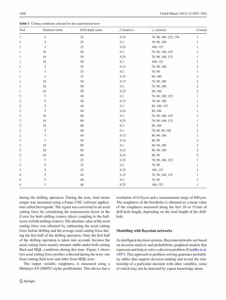
The complete experimental test included 90 different con-ditions. All the tests were repeated to increase the amount ofdata to obtain a data set of 180 records, the incomplete recordswere removed leaving a training data set of 169 records.Table 1 shows the selected values for each variable in eachtest. A further input variable, axial cutting force, is unknowna priori and is therefore not included in Table 1.

All the drill-holes were drilled in one step, without a pilothole. Each hole was drilled with a constant spindle speedand feed per revolution. The tests with working fluid wereperformed with a working fluid pressure of 23 bars, usingHoughton HOCUT B-750 cutting oil at 5%. The tests underMQL conditions were performed with air pressure at 4 barsusing LUXOL A15 cutting oil.

The tests were performed along the Z-axis of the millingcentres. The torque provided in real time by the feed motorof the Z-axis would therefore provide the axial cutting force

123

1896 J Intell Manuf (2012) 23:1893–1902

Table 1 Cutting conditions selected for the experimental tests

Tool Diameter (mm) Drill depth (mm) f (mm/rev) vc (m/min) Coolant

1 5 25 0.15 70, 90, 100, 125, 130 1

1 5 25 0.2 70, 90, 100 1

1 5 25 0.25 100, 125 1

1 10 50 0.2 70, 90, 100, 125 1

1 10 50 0.25 70, 90, 100, 125 1

1 10 50 0.3 100, 125 1

1 5 25 0.15 70, 90, 100 2

1 5 25 0.2 70, 90 2

1 5 25 0.25 90, 100 2

1 10 50 0.15 70, 90, 100 2

1 10 50 0.2 70, 90, 100 2

1 10 50 0.25 90, 100 2

2 5 40 0.1 70, 80, 100, 125 1

2 5 40 0.15 70, 80, 100 1

2 5 40 0.2 80, 100, 125 1

2 5 40 0.25 80, 100 1

2 10 80 0.2 70, 90, 100, 125 1

2 10 80 0.25 70, 90, 100, 125 1

2 10 80 0.3 90, 100 1

2 5 40 0.1 70, 80, 90, 100 2

2 5 40 0.12 80, 90, 100 2

2 5 40 0.14 80, 90 2

2 10 80 0.1 80, 90, 100 2

2 10 80 0.12 80, 90, 100 2

2 10 80 0.14 80, 90 2

3 5 25 0.15 70, 90, 100, 125 1

3 5 25 0.2 70, 90 1

3 5 25 0.25 100, 125 1

4 5 40 0.15 70, 90, 100, 125 1

4 5 40 0.2 70, 90 1

4 5 40 0.25 100, 125 1

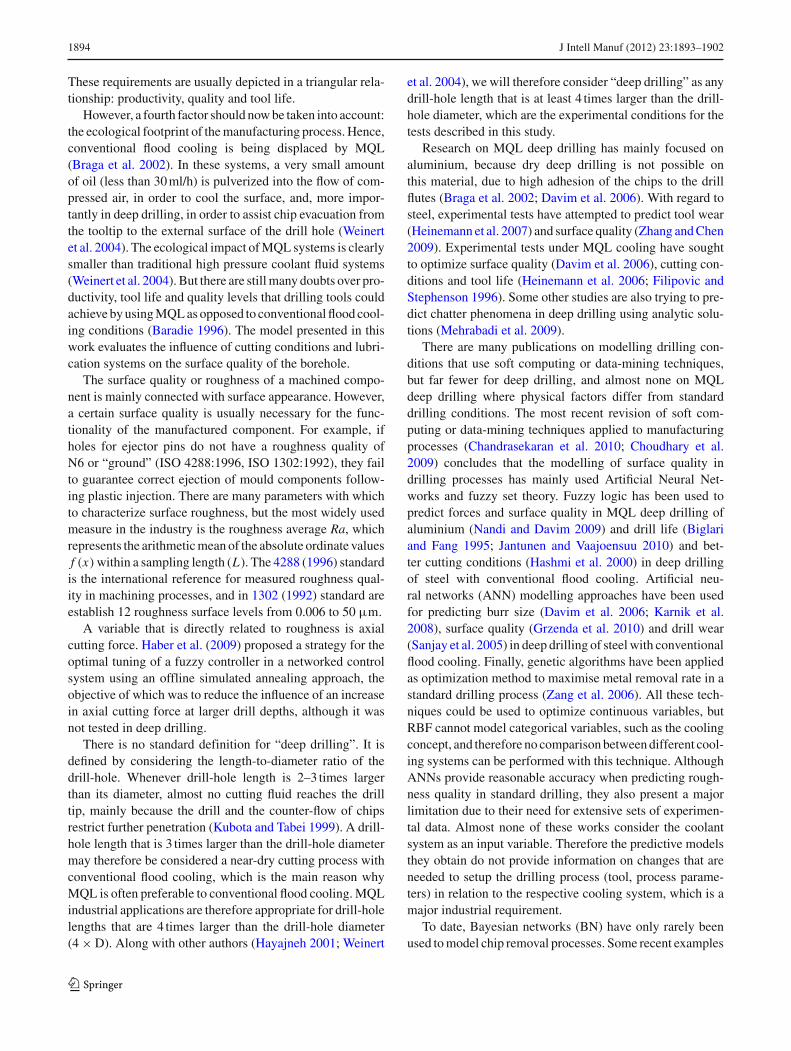
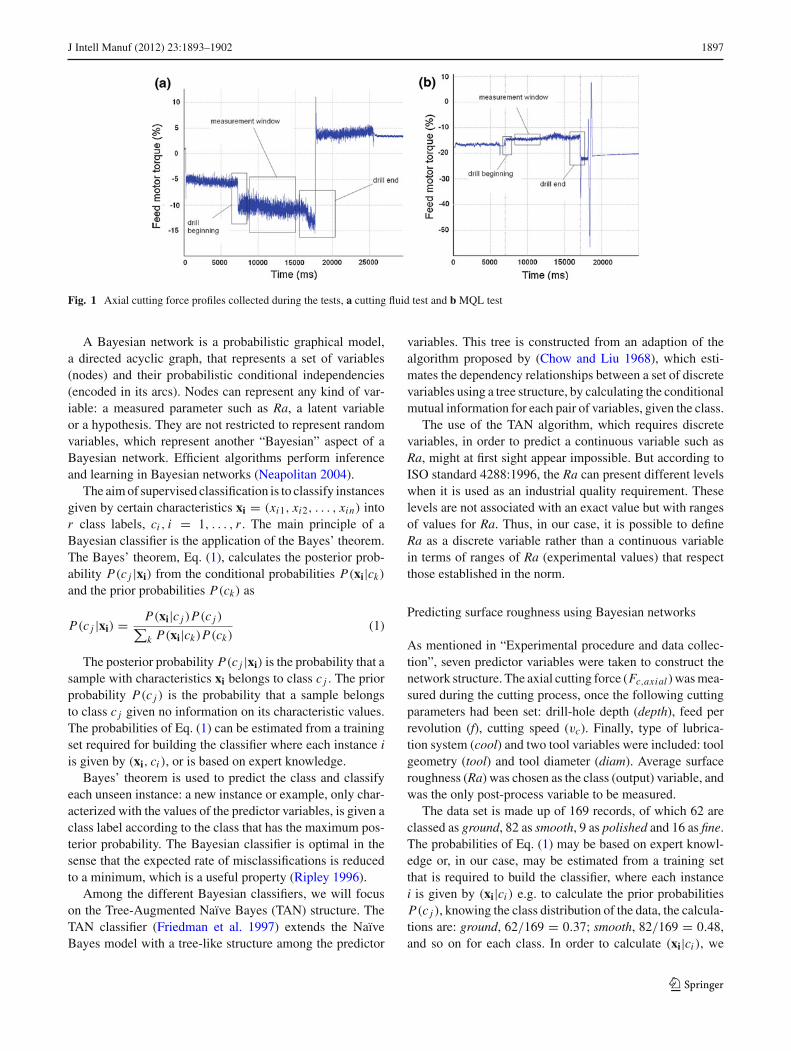
during the drilling operation. During the tests, feed motortorque was measured using a Fanuc CNC software applica-tion called Servoguide. The signal was converted to an axialcutting force by considering the transmission factor in theZ-axis for both milling centres (direct coupling to the ball-screw in both milling centres). The absolute value of the axialcutting force was obtained by subtracting the axial cuttingforce before drilling and the average axial cutting force dur-ing the first half of the drilling operation. Only the first halfof the drilling operation is taken into account, because theaxial cutting force mainly remains stable under both cuttingfluid and MQL conditions during this time. Figure 1 showstwo axial cutting force profiles collected during the tests: onefrom cutting fluid tests and other from MQL tests.

The output variable, roughness, is measured using aMitutoyo SV-2000N2 stylus profilometer. This device has a

resolution of 0.01µm and a measurement range of 800 µm.The roughness of the boreholes is obtained as a mean valueof the roughness measured along the first 10 or 15 mm ofdrill-hole length, depending on the total length of the drill-hole.

Modelling with Bayesian networks

As intelligent decision systems, Bayesian networks are basedon decision analysis and probabilistic graphical models thatrepresent and help to solve a decision problem (Castillo et al.1997). This approach to problem solving generates probabil-ity tables that support decision-making and reveal the rela-tionship of a particular decision with other variables, someof which may not be detected by expert knowledge alone.

123

J Intell Manuf (2012) 23:1893–1902 1897

Fig. 1 Axial cutting force profiles collected during the tests, a cutting fluid test and b MQL test

A Bayesian network is a probabilistic graphical model,a directed acyclic graph, that represents a set of variables(nodes) and their probabilistic conditional independencies(encoded in its arcs). Nodes can represent any kind of var-iable: a measured parameter such as Ra, a latent variableor a hypothesis. They are not restricted to represent randomvariables, which represent another “Bayesian” aspect of aBayesian network. Efficient algorithms perform inferenceand learning in Bayesian networks (Neapolitan 2004).

The aim of supervised classification is to classify instancesgiven by certain characteristics xi = (xi1, xi2, . . . , xin) intor class labels, ci , i = 1, . . . , r . The main principle of aBayesian classifier is the application of the Bayes’ theorem.The Bayes’ theorem, Eq. (1), calculates the posterior prob-ability P(c j |xi) from the conditional probabilities P(xi|ck)

and the prior probabilities P(ck) as

P(c j |xi) = P(xi|c j )P(c j )∑

k P(xi|ck)P(ck)(1)

The posterior probability P(c j |xi) is the probability that asample with characteristics xi belongs to class c j . The priorprobability P(c j ) is the probability that a sample belongsto class c j given no information on its characteristic values.The probabilities of Eq. (1) can be estimated from a trainingset required for building the classifier where each instance iis given by (xi, ci ), or is based on expert knowledge.

Bayes’ theorem is used to predict the class and classifyeach unseen instance: a new instance or example, only char-acterized with the values of the predictor variables, is given aclass label according to the class that has the maximum pos-terior probability. The Bayesian classifier is optimal in thesense that the expected rate of misclassifications is reducedto a minimum, which is a useful property (Ripley 1996).

Among the different Bayesian classifiers, we will focuson the Tree-Augmented Naïve Bayes (TAN) structure. TheTAN classifier (Friedman et al. 1997) extends the NaïveBayes model with a tree-like structure among the predictor

variables. This tree is constructed from an adaption of thealgorithm proposed by (Chow and Liu 1968), which esti-mates the dependency relationships between a set of discretevariables using a tree structure, by calculating the conditionalmutual information for each pair of variables, given the class.

The use of the TAN algorithm, which requires discretevariables, in order to predict a continuous variable such asRa, might at first sight appear impossible. But according toISO standard 4288:1996, the Ra can present different levelswhen it is used as an industrial quality requirement. Theselevels are not associated with an exact value but with rangesof values for Ra. Thus, in our case, it is possible to defineRa as a discrete variable rather than a continuous variablein terms of ranges of Ra (experimental values) that respectthose established in the norm.

Predicting surface roughness using Bayesian networks

As mentioned in “Experimental procedure and data collec-tion”, seven predictor variables were taken to construct thenetwork structure. The axial cutting force (Fc,axial ) was mea-sured during the cutting process, once the following cuttingparameters had been set: drill-hole depth (depth), feed perrevolution (f), cutting speed (vc). Finally, type of lubrica-tion system (cool) and two tool variables were included: toolgeometry (tool) and tool diameter (diam). Average surfaceroughness (Ra) was chosen as the class (output) variable, andwas the only post-process variable to be measured.

The data set is made up of 169 records, of which 62 areclassed as ground, 82 as smooth, 9 as polished and 16 as fine.The probabilities of Eq. (1) may be based on expert knowl-edge or, in our case, may be estimated from a training setthat is required to build the classifier, where each instancei is given by (xi|ci ) e.g. to calculate the prior probabilitiesP(c j ), knowing the class distribution of the data, the calcula-tions are: ground, 62/169 = 0.37; smooth, 82/169 = 0.48,and so on for each class. In order to calculate (xi|ci ), we

123

1898 J Intell Manuf (2012) 23:1893–1902

Table 2 Variables used and their respective assigned intervals

State tool diam (mm) depth (mm) f (mm/rev) Fc,axial (N) vc (m/ min) cool Ra (µm)

1 1 5 25 [0.1,0.15) [0,550) [70,80) 1 [0.25,0.35)

polished

2 2 10 40 [0.15, 0.2) [550,850) [80,90) 2 [0.35,0.75)

ground

3 3 50 [0.2, 0.25) [850,1150) [90,100) [0.75,1.4)

smooth

4 4 80 [0.25,0.3) [1150,1450) [100,110) [1.4, 2.1)

fine

5 [1450,1750) [110,120)

6 [1750,2050) [120,130)

7 [2050, 2350) [130,160)

8 [2350,2800)

continue to use ground as the class value. In this case, we shallcalculate P(depth|Ra = ground). Knowing that the dataset has 62 records classed as ground, as we wish to calculatethe probability of the variable depth, given class as ground.The amount of data at each depth is examined: in this exam-ple, for ground at depth 25: records, probability calculated as28/62 = 0.45; depth 40: 9 records, probability 9/62 = 0.15;depth 50: 18 records, probability 18/62 = 0.28 and depth80: 7 records, probability 7/62 = 0.11. This example illus-trates the method of calculating the probabilities from thetraining data.

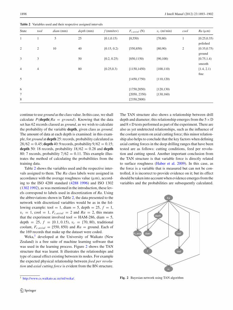
Table 2 shows the variables used and the respective inter-vals assigned to them. The Ra class labels were assigned inaccordance with the average roughness value (µm), accord-ing to the ISO 4288 standard (4288 1996) and ISO 1302(1302 1992), as was mentioned in the introduction, these lev-els correspond to labels used in discretization of Ra. Usingthe abbreviations shown in Table 2, the data presented to thenetwork with discretized variables would be as in the fol-lowing example: tool = 1, diam = 5, depth = 25, f = 1,vc = 1, cool = 1, Fc,axial = 2 and Ra = 2, this meansthat the experiment involved tool = HAM-286, diam = 5,depth = 25, f = [0.1, 0.15), vc = [70, 80), traditionalcoolant, Fc,axial = [550, 850) and Ra = ground. Each ofthe 169 records that make up the dataset were coded.

Weka,1 developed at the University of Waikato (NewZealand) is a free suite of machine learning software thatwas used in the learning process. Figure 2 shows the TANstructure that was learnt. It illustrates the relationships andtype of causal effect existing between its nodes. For examplethe expected physical relationship between feed per revolu-tion and axial cutting force is evident from the BN structure.

1 http://www.cs.waikato.ac.nz/ml/weka/.

The TAN structure also shows a relationship between drilldepth and diameter; this relationship emerges from the 5×Dand 8×D tests performed as part of the experiment. There arealso as yet undetected relationships, such as the influence ofthe coolant system on axial cutting force; this minor relation-ship also helps to conclude that the key factors when definingaxial cutting forces in the deep drilling ranges that have beentested are as follows: cutting conditions, feed per revolu-tion and cutting speed. Another important conclusion fromthe TAN structure is that variable force is directly relatedto surface roughness (Haber et al. 2009). In this case, asthe force is a variable that is measured but can not be con-trolled, it is incorrect to provide evidence on it; but its effectshould be taken into account when evidence emerges from thevariables and the probabilities are subsequently calculated.

Fig. 2 Bayesian network using TAN algorithm

123

J Intell Manuf (2012) 23:1893–1902 1899

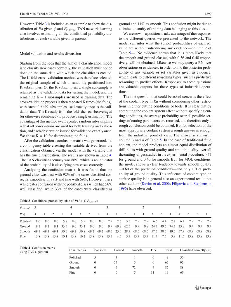
However, Table 3 is included as an example to show the dis-tribution of Ra given f and Fc,axial . TAN network learningalso involves estimating all the conditional probability dis-tributions of each variable given its parents.

Model validation and results discussion

Starting from the idea that the aim of a classification modelis to classify new cases correctly, the validation must not bedone on the same data with which the classifier is created.The K-fold cross-validation method was therefore selected,the original sample of which is randomly partitioned intoK subsamples. Of the K subsamples, a single subsample isretained as the validation data for testing the model, and theremaining K − 1 subsamples are used as training data. Thecross-validation process is then repeated K times (the folds),with each of the K subsamples used exactly once as the vali-dation data. The K results from the folds then can be averaged(or otherwise combined) to produce a single estimation. Theadvantage of this method over repeated random sub-samplingis that all observations are used for both training and valida-tion, and each observation is used for validation exactly once.We chose K = 10 for determining the folds.

After the validation a confusion matrix was generated, i.e.a contingency table crossing the variable derived from theclassification obtained via the model with the variable thathas the true classification. The results are shown in Table 4.The TAN classifier accuracy was 86%, which is an indicatorof the probability of it classifying new cases correctly.

Analyzing the confusion matrix, it was found that theground class was best with 92% of the cases classified cor-rectly, smooth with 88% and fine with 69%. However, therewas greater confusion with the polished class which had 56%well classified, while 33% of the cases were classified as

ground and 11% as smooth. This confusion might be due toa limited quantity of training data belonging to this class.

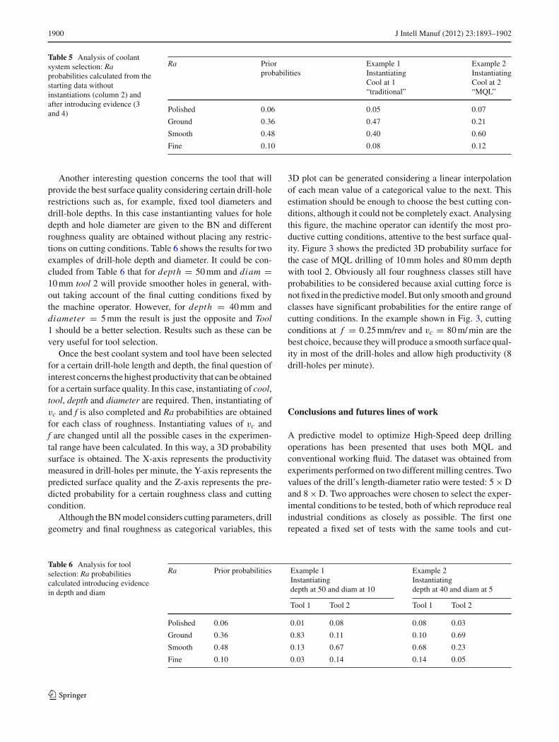
We are now in a position to take advantage of the responsesto the different queries we presented to the network. Themodel can infer what the (prior) probabilities of each Ravalue are without introducing any evidence—column 2 ofTable 5—. No evidence shows that it is more likely thatthe smooth and ground classes, with 0.36 and 0.48 respec-tively, will be obtained. Likewise we may query a BN overobservations or evidences, in order to find the posterior prob-ability of any variable or set variables given as evidence,which leads to different reasoning types, such as predictivereasoning to predict effects. Responses to these questionsare valuable outputs for these types of industrial opera-tions.

The first question that could be asked concerns the effectof the coolant type in Ra without considering other restric-tions in either cutting conditions or tools. It is clear that bycomputing the coolant system effect without specifying cut-ting conditions, the average probability over all possible set-tings of cutting parameters are returned, and therefore only arough conclusion could be obtained. But for selection of themost appropriate coolant system a rough answer is enoughfrom the industrial point of view. The answer is shown incolumn 3 and 4 of Table 5. In the case of traditional fluidcoolant, the model predicts an almost equal distribution ofdrill-holes with ground quality and smooth quality over allthe cutting ranges studied in the experimental procedure, 0.47for ground and 0.40 for smooth. But, for MQL conditions,the model shows a clear tendency towards smooth quality−0.60 of the predicted conditions—and only a 0.21 prob-ability of ground quality. This influence of coolant type onsurface quality is in general also an experimental result thatother authors (Davim et al. 2006; Filipovic and Stephenson1996) have observed.

Table 3 Conditional probability table of P(Ra| f, Fc,axial)

Fc,axial 5 4 3 2 1

Ra/f 4 3 2 1 4 3 2 1 4 3 2 1 4 3 2 1 4 3 2 1

Polished 8.0 8.0 8.0 5.8 8.0 5.9 8.0 8.0 7.9 2.6 3.3 7.9 7.9 6.6 4.4 2.2 6.7 7.9 7.9 7.9

Ground 9.1 9.1 9.1 33.5 9.0 33.1 9.0 9.0 9.9 69.8 62.3 9.9 9.8 24.7 49.6 74.7 23.8 9.4 9.4 9.4

Smooth 69.1 69.1 69.1 50.6 69.2 50.8 69.2 69.2 68.5 23.0 28.7 68.5 68.6 57.3 38.5 19.3 57.9 68.9 68.9 68.9

Fine 13.8 13.8 13.8 10.1 13.8 10.2 13.8 13.8 13.7 4.6 5.7 13.7 13.7 11.4 7.5 3.8 11.6 13.8 13.8 13.8

Table 4 Confusion matrixusing TAN algorithm Classified as Polished Ground Smooth Fine Total Classified correctly (%)

Polished 5 3 1 0 9 56

Ground 0 57 5 0 62 92

Smooth 0 6 72 4 82 88

Fine 0 0 5 11 16 69

123

1900 J Intell Manuf (2012) 23:1893–1902

Table 5 Analysis of coolantsystem selection: Raprobabilities calculated from thestarting data withoutinstantiations (column 2) andafter introducing evidence (3and 4)

Ra Prior Example 1 Example 2probabilities Instantiating Instantiating

Cool at 1 Cool at 2“traditional” “MQL”

Polished 0.06 0.05 0.07

Ground 0.36 0.47 0.21

Smooth 0.48 0.40 0.60

Fine 0.10 0.08 0.12

Another interesting question concerns the tool that willprovide the best surface quality considering certain drill-holerestrictions such as, for example, fixed tool diameters anddrill-hole depths. In this case instantianting values for holedepth and hole diameter are given to the BN and differentroughness quality are obtained without placing any restric-tions on cutting conditions. Table 6 shows the results for twoexamples of drill-hole depth and diameter. It could be con-cluded from Table 6 that for depth = 50 mm and diam =10 mm tool 2 will provide smoother holes in general, with-out taking account of the final cutting conditions fixed bythe machine operator. However, for depth = 40 mm anddiameter = 5 mm the result is just the opposite and Tool1 should be a better selection. Results such as these can bevery useful for tool selection.

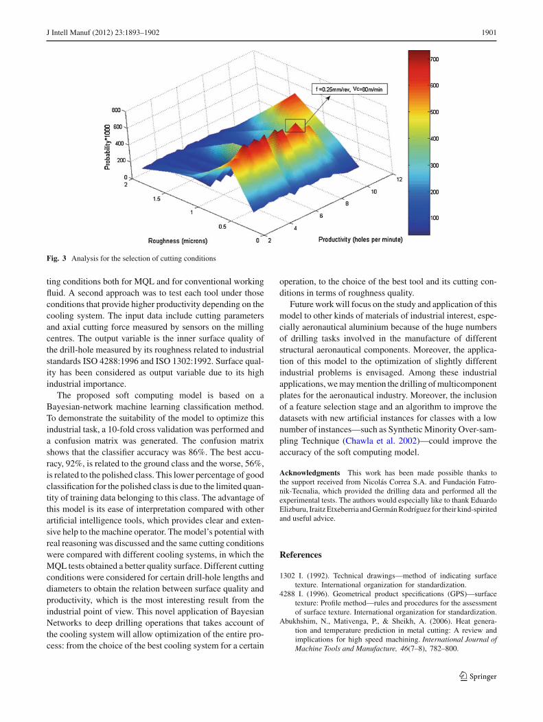
Once the best coolant system and tool have been selectedfor a certain drill-hole length and depth, the final question ofinterest concerns the highest productivity that can be obtainedfor a certain surface quality. In this case, instantiating of cool,tool, depth and diameter are required. Then, instantiating ofvc and f is also completed and Ra probabilities are obtainedfor each class of roughness. Instantiating values of vc andf are changed until all the possible cases in the experimen-tal range have been calculated. In this way, a 3D probabilitysurface is obtained. The X-axis represents the productivitymeasured in drill-holes per minute, the Y-axis represents thepredicted surface quality and the Z-axis represents the pre-dicted probability for a certain roughness class and cuttingcondition.

Although the BN model considers cutting parameters, drillgeometry and final roughness as categorical variables, this

3D plot can be generated considering a linear interpolationof each mean value of a categorical value to the next. Thisestimation should be enough to choose the best cutting con-ditions, although it could not be completely exact. Analysingthis figure, the machine operator can identify the most pro-ductive cutting conditions, attentive to the best surface qual-ity. Figure 3 shows the predicted 3D probability surface forthe case of MQL drilling of 10 mm holes and 80 mm depthwith tool 2. Obviously all four roughness classes still haveprobabilities to be considered because axial cutting force isnot fixed in the predictive model. But only smooth and groundclasses have significant probabilities for the entire range ofcutting conditions. In the example shown in Fig. 3, cuttingconditions at f = 0.25 mm/rev and vc = 80 m/ min are thebest choice, because they will produce a smooth surface qual-ity in most of the drill-holes and allow high productivity (8drill-holes per minute).

Conclusions and futures lines of work

A predictive model to optimize High-Speed deep drillingoperations has been presented that uses both MQL andconventional working fluid. The dataset was obtained fromexperiments performed on two different milling centres. Twovalues of the drill’s length-diameter ratio were tested: 5 × Dand 8 × D. Two approaches were chosen to select the exper-imental conditions to be tested, both of which reproduce realindustrial conditions as closely as possible. The first onerepeated a fixed set of tests with the same tools and cut-

Table 6 Analysis for toolselection: Ra probabilitiescalculated introducing evidencein depth and diam

Ra Prior probabilities Example 1 Example 2Instantiating Instantiatingdepth at 50 and diam at 10 depth at 40 and diam at 5

Tool 1 Tool 2 Tool 1 Tool 2

Polished 0.06 0.01 0.08 0.08 0.03

Ground 0.36 0.83 0.11 0.10 0.69

Smooth 0.48 0.13 0.67 0.68 0.23

Fine 0.10 0.03 0.14 0.14 0.05

123

J Intell Manuf (2012) 23:1893–1902 1901

Fig. 3 Analysis for the selection of cutting conditions

ting conditions both for MQL and for conventional workingfluid. A second approach was to test each tool under thoseconditions that provide higher productivity depending on thecooling system. The input data include cutting parametersand axial cutting force measured by sensors on the millingcentres. The output variable is the inner surface quality ofthe drill-hole measured by its roughness related to industrialstandards ISO 4288:1996 and ISO 1302:1992. Surface qual-ity has been considered as output variable due to its highindustrial importance.

The proposed soft computing model is based on aBayesian-network machine learning classification method.To demonstrate the suitability of the model to optimize thisindustrial task, a 10-fold cross validation was performed anda confusion matrix was generated. The confusion matrixshows that the classifier accuracy was 86%. The best accu-racy, 92%, is related to the ground class and the worse, 56%,is related to the polished class. This lower percentage of goodclassification for the polished class is due to the limited quan-tity of training data belonging to this class. The advantage ofthis model is its ease of interpretation compared with otherartificial intelligence tools, which provides clear and exten-sive help to the machine operator. The model’s potential withreal reasoning was discussed and the same cutting conditionswere compared with different cooling systems, in which theMQL tests obtained a better quality surface. Different cuttingconditions were considered for certain drill-hole lengths anddiameters to obtain the relation between surface quality andproductivity, which is the most interesting result from theindustrial point of view. This novel application of BayesianNetworks to deep drilling operations that takes account ofthe cooling system will allow optimization of the entire pro-cess: from the choice of the best cooling system for a certain

operation, to the choice of the best tool and its cutting con-ditions in terms of roughness quality.

Future work will focus on the study and application of thismodel to other kinds of materials of industrial interest, espe-cially aeronautical aluminium because of the huge numbersof drilling tasks involved in the manufacture of differentstructural aeronautical components. Moreover, the applica-tion of this model to the optimization of slightly differentindustrial problems is envisaged. Among these industrialapplications, we may mention the drilling of multicomponentplates for the aeronautical industry. Moreover, the inclusionof a feature selection stage and an algorithm to improve thedatasets with new artificial instances for classes with a lownumber of instances—such as Synthetic Minority Over-sam-pling Technique (Chawla et al. 2002)—could improve theaccuracy of the soft computing model.

Acknowledgments This work has been made possible thanks tothe support received from Nicolás Correa S.A. and Fundación Fatro-nik-Tecnalia, which provided the drilling data and performed all theexperimental tests. The authors would especially like to thank EduardoElizburu, Iraitz Etxeberria and Germán Rodríguez for their kind-spiritedand useful advice.

References

1302 I. (1992). Technical drawings—method of indicating surfacetexture. International organization for standardization.

4288 I. (1996). Geometrical product specifications (GPS)—surfacetexture: Profile method—rules and procedures for the assessmentof surface texture. International organization for standardization.

Abukhshim, N., Mativenga, P., & Sheikh, A. (2006). Heat genera-tion and temperature prediction in metal cutting: A review andimplications for high speed machining. International Journal ofMachine Tools and Manufacture, 46(7–8), 782–800.

123

1902 J Intell Manuf (2012) 23:1893–1902

Baradie, M. E. (1996). Cutting fluids: Part i. Characterisation. Journalof Materials Processing Technology, 56, 786–797.

Biermann, D., Kersting, M., & Kessler, N. (2009). Process adaptedstructure optimization of deep hole drilling tools. CIRP AnnalsManufacturing Technology, 58(1), 89–92.

Biglari, F., & Fang, X. (1995). Real-time fuzzy-logic control formaximizing the tool life of small-diameter drills. Fuzzy Sets andSystems, 72(1), 91–101.

Braga, D., Diniz, A., Miranda, G., & Coppinni, N. (2002). Usinga minimum quantity of lubrication and a diamond coated toolin drilling of aluminum-silicon alloys. Journal of Materials Pro-cessing Technology, 122, 127–138.

Castillo, E., Gutiérrez, E., & Hadi, A. (1997). Expert systems andprobabilistic network models. NY: Springer.

Chandrasekaran, M., Muralidhar, M., Krishna, C. M., & Dixit, U. S.(2010). Application of soft computing techniques in machin-

ing performance prediction and optimization: A literaturereview. International Journal of Advanced Manufacturing Tech-nologie, 46, 445–464.

Chawla, N., Bowyer, K., Hall, L., & Kegelmeyer, W. (2002). Smote:Synthetic minority over-sampling technique. Journal of ArtificialIntelligence Research, 16, 321–357.

Choudhary, A., Harding, J., & Tiwari, M. (2009). Data mining inmanufacturing: A review based on the kind of knowledge. Journalof Intelligent Manufacturing, 20(5), 501–521.

Chow, C., & Liu, C. (1968). Approximating discrete probability distri-butions. IEEE Transactions on Information Theory, 14, 462–467.

Coldwell, H., Woods, R., Paul, M., Koshy, P., Dewes, R., & Aspinwall,D. (2003). Rapid machining of hardened aisi h13 and d2 moulds,dies and press tools. Journal of Materials Processing Technol-ogy, 135, 301–311.

Correa, M., Bielza, C., de Ramirez, J. M., & Alique, J. (2008). Abayesian network model for surface roughness prediction inthe machining process. International Journal of Systems Sci-ence, 39(12), 1181–1192.

Correa, M., Bielza, C., & Pamies-Teixeira, J. (2009). Comparisonof bayesian networks and artificial neural networks for qualitydetection in a machining process. Expert Systems with Applica-tions, 36, 7270–7279.

Davim, J., Sreejith, P., Gomes, R., & Peixoto, C. (2006). Experimentalstudies on drilling of aluminium (aa1050) under dry, minimumquantity of lubricant, and flood-lubricated conditions. Proceed-ings of the Institution of Mechanical Engineers Part B-Journal ofEngineering Manufacture, 220(10), 1605–1611.

Filipovic, A., & Stephenson, D. (1996). Minimum quantity lubrication(mql) applications in automotive power-train machining. Mechan-ical Science and Technology, 10, 3–22.

Friedman, N., Geiger, D., & Goldszmit, M. (1997). Bayesian networkclassifiers. Machine Learning, 29, 131–161.

Grzenda, M., Bustillo, A., Zawistowski, P. (2010). A soft comput-ing system using intelligent imputation strategies for roughnessprediction in deep drilling. Journal of Intelligent Manufacturing,1–11. Article in Press.

Haber, R., Haber-Haber, R., Jimenez, A., & Galan, R. (2009). Anoptimal fuzzy control system in a network environment based onsimulated annealing. An application to a drilling process. AppliedSoft Computing Journal, 9(3), 889–895.

Hashmi, K., Graham, I., & Mills, B. (2000). Fuzzy logic based dataselection for the drilling process. Journal of Materials ProcessingTechnology, 108(1), 55–61.

Hayajneh, N. (2001). Hole quality in deep hole drilling source. Mate-rials and Manufacturing Processes, 16(2), 147–164.

Heinemann, R., Hinduja, S., Barrow, G., & Petuelli, G. (2006). Effect ofmql on the tool life of small twist drills in deep-hole drilling. Inter-national Journal of Machine Tools and Manufacture, 46(1), 1–6.

Heinemann, R., Hinduja, S., & Barrow, G. (2007). Use of processsignals for tool wear progression sensing in drilling small deepholes. International Journal of Advanced Manufacturing Technol-ogy, 33(3–4), 243–250.

Jantunen, E., & Vaajoensuu, E. (2010). Self adaptive diagnosis oftool wear with a microcontroller. Journal of Intelligent Manufac-turing, 21(2), 223–230.

Karnik, S. R., Gaitonde, V. N., & Davim, J. P. (2008). A comparativestudy of the ann and rsm modeling approaches for predicting burrsize in drilling. International Journal of Advanced ManufacturingTechnology, 38(9–10), 868–883.

Kubota, H., & Tabei, H. (1999). Drilling of a small and deep holeusing a twist drill. Transactions of the Japan Society of MechanicalEngineers, Part C, 62(601), 3691–3697.

Lorincz, J. (2006). Drilling to the limits: Innovative holemaking toolscan improve cycle time, reduce cost per hole. ManufacturingEngineering, 136(4), 71–75.

Mehrabadi, I., Nouri, M., & Madoliat, R. (2009). Investigating chat-ter vibration in deep drilling, including process damping andthe gyroscopic effect. International Journal of Machine Tools &Manufacture, 49(12–13), 939–946.

Nandi, A., & Davim, J. (2009). A study of drilling performances withminimum quantity of lubricant using fuzzy logic rules. Mecha-tronics, 19(2), 218–232.

Neapolitan, R. (2004). Learning bayesian networks. EnglewoodCliffs: Prentice Hall.

Ripley, B. (1996). Pattern recognition and neural networks. Cam-bridge: Cambridge University Press.

Sanjay, C., Neema, M., & Chin, C. (2005). Modeling of tool wear indrilling by statistical analysis and artificial neural network. Jour-nal of Materials Processing Technology, 170(3), 494–500.

Weinert, K., Inasaki, I., Sutherland, J., & Wakabayashi, T. (2004).Dry machining and minimum quantity lubrication. Annals CIRP,53(2), 511–537.

Zang, J., Liang, S., Yao, J., Chen, J., & Hang, J. (2006). Evolution-ary optimization of machining processes. Journal of IntelligentManufacturing, 17(2), 203–215.

Zhang, J., & Chen, J. (2009). Surface roughness optimization in adrilling operation using the taguchi design method. Materialsand Manufacturing Processes, 24(4), 459–467.

123