us grain sorghum in japan - ttu dspace home
TRANSCRIPT
US Grain Sorghum in Japan: Understanding and Measuring a Declining Market Share
by
Kazuyoshi Ishida, MA Economics
A Dissertation
In
Department of Agricultural and Applied Economics
Submitted to the Graduate Faculty of Texas Tech University in
Partial Fulfillment of the Requirements for
the Degree of Doctor of Philosophy
Approved
Jaime E. Malaga, Ph.D.
Chair of Committee
Darren Hudson, Ph.D
Benaissa Chidmi, Ph.D
Rashid Al-Hmoud, Ph D
Mark Sheridan Dean of the Graduate School
May 2017

Copyright 2017, Kazuyoshi Ishida

Texas Tech University, Kazuyoshi Ishida, May 2017
ii
ACKNOWLEDGEMENT
I would like to express the deepest appreciation to my committee chair
Professor Dr. Malaga, who are knowledgeable about my dissertation topic and give
me useful suggestions for developing my research. I would like to thank to my
committee member, Dr. Chidmi, who help me conduct an empirical analysis and
estimate the parameters of the models in this dissertation. I appreciated the suggestions
and comments from Dr. Hudson in the committee meeting and the proposal defense.
His suggestions and comments are very important in improving my dissertation. I need
to thank Dr. Al-Hmoud for participating in my dissertation and giving useful
comments for developing this dissertation.
Texas Tech University, Kazuyoshi Ishida, May 2017
iii
Table of Contents
ACKNOWLEDGEMENT ................................................................................... ii
ABSTRACT .......................................................................................................... v
LIST OF TABLES .............................................................................................. vi
LIST OF FIGURES ........................................................................................... vii
I. CHAPTER 1 AN APPROPRIATE METHODOLOGY FOR THE DEMAND ANALYSIS OF US SORGHUM IN THE JAPANESE FEEDING GRAIN MARKET ............................................................................................................... 1
Abstract ............................................................................................................. 1
Introduction ....................................................................................................... 2
The Effect of Quality Differential on Demand ................................................. 4
Identification of Appropriate Models................................................................ 9
Separability Condition ................................................................................... 17
Conclusion ...................................................................................................... 20
II. CHAPTER2 WHY THE MARKET SHARE OF US GRAIN SORGHUM HAS DECLINED IN ITS JAPANESE MARKET? ......................................... 21
Abstract ........................................................................................................... 21
Introduction ..................................................................................................... 22
Litearture Review ............................................................................................ 25
Conceptual Framework ................................................................................... 26
Empirical Framework...................................................................................... 29
Data Description........................................................................................ 30 Econometric Model ................................................................................... 31 Structure Breakpoint Identification ........................................................... 34 A Drastic Increase in Chinese Imports of Grain Sorghum ....................... 35 Quality Elasticities .................................................................................... 37 Random Estimation of Elasticities ............................................................ 38
Results ............................................................................................................. 40
Result of the AIDS Model Regression ...................................................... 40 Result of the Translog Model Regression ............................................... 44 Separability Condition .............................................................................. 46 A Drastic Increase in Chinese Imports of Grain Sorghum ....................... 47
Texas Tech University, Kazuyoshi Ishida, May 2017
iv
Quality Elasticities .................................................................................... 49 Random Estimations of Elasticities .......................................................... 50 An Analysis of the Effect of the Feed Efficiency using a Bayesian SUR 50 An Analysis of the Effect of Chinese Import of Grain Sorghum using a Bayesian SUR ........................................................................................... 52
Conclusion ...................................................................................................... 53
REFERENCE ...................................................................................................... 57
APPENDICES A. FIGURES IN THE FIRST CHAPTER ........................................................ 60
B. FIGURES IN THE SECOND CHAPTER ................................................... 61
C.THE POSTERIOR DISTRIBUTIONS ........................................................ 65
Texas Tech University, Kazuyoshi Ishida, May 2017
v
ABSTRACT
The purpose of this dissertation is to explore the causes of the market share
loss of US grain sorghum in the Japanese market. The first chapter of the dissertation
identifies the appropriate methodology for an analysis of the demand for US grain
sorghum in the Japanese market by taking into consideration recent market trends. The
second chapter conducts an empirical analysis to reveal why US grain sorghum has
been losing share in the Japanese market based on the appropriate methodology
identified in the first chapter.
Texas Tech University, Kazuyoshi Ishida, May 2017
vi
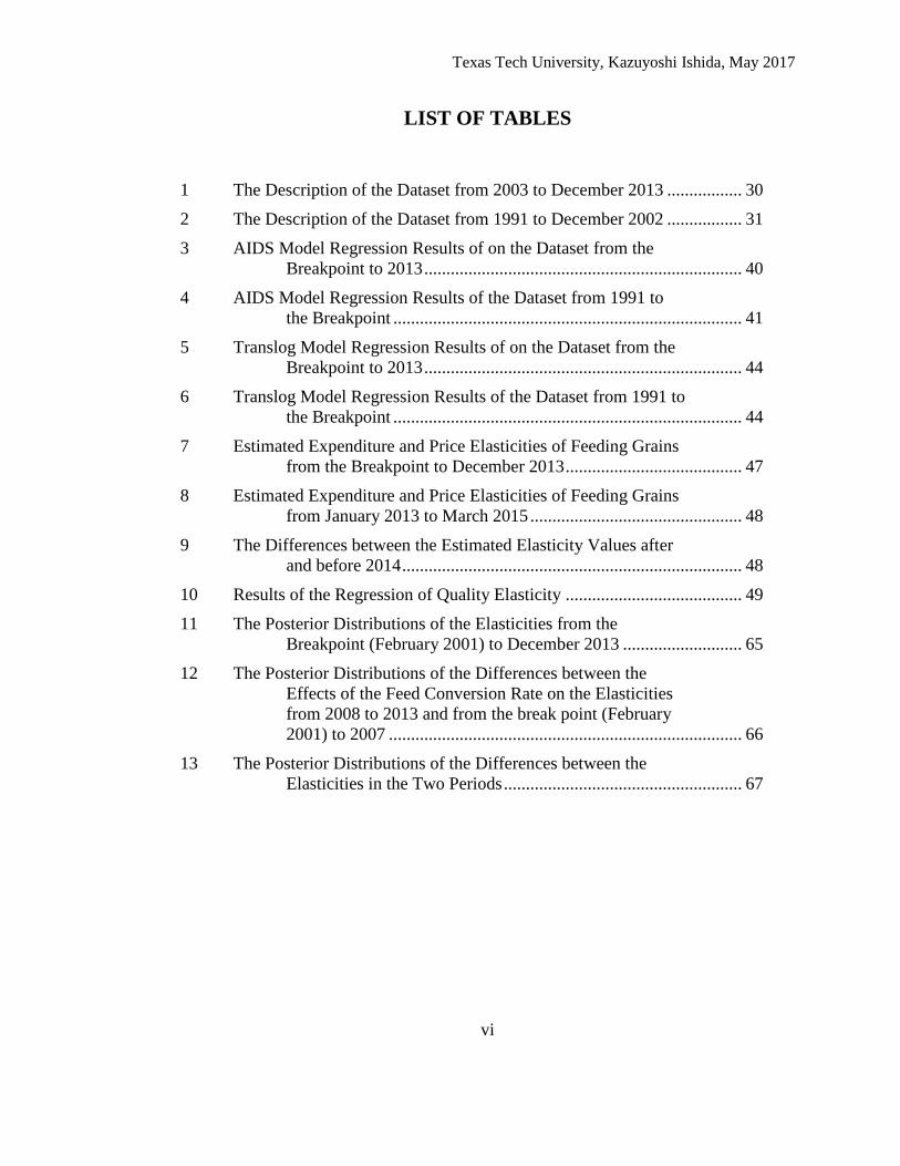
LIST OF TABLES
1 The Description of the Dataset from 2003 to December 2013 ................. 30
2 The Description of the Dataset from 1991 to December 2002 ................. 31
3 AIDS Model Regression Results of on the Dataset from the Breakpoint to 2013 ........................................................................ 40
4 AIDS Model Regression Results of the Dataset from 1991 to the Breakpoint ............................................................................... 41
5 Translog Model Regression Results of on the Dataset from the Breakpoint to 2013 ........................................................................ 44
6 Translog Model Regression Results of the Dataset from 1991 to the Breakpoint ............................................................................... 44
7 Estimated Expenditure and Price Elasticities of Feeding Grains from the Breakpoint to December 2013 ........................................ 47
8 Estimated Expenditure and Price Elasticities of Feeding Grains from January 2013 to March 2015 ................................................ 48
9 The Differences between the Estimated Elasticity Values after and before 2014 ............................................................................. 48
10 Results of the Regression of Quality Elasticity ........................................ 49
11 The Posterior Distributions of the Elasticities from the Breakpoint (February 2001) to December 2013 ........................... 65
12 The Posterior Distributions of the Differences between the Effects of the Feed Conversion Rate on the Elasticities from 2008 to 2013 and from the break point (February 2001) to 2007 ................................................................................ 66
13 The Posterior Distributions of the Differences between the Elasticities in the Two Periods ...................................................... 67
Texas Tech University, Kazuyoshi Ishida, May 2017
vii
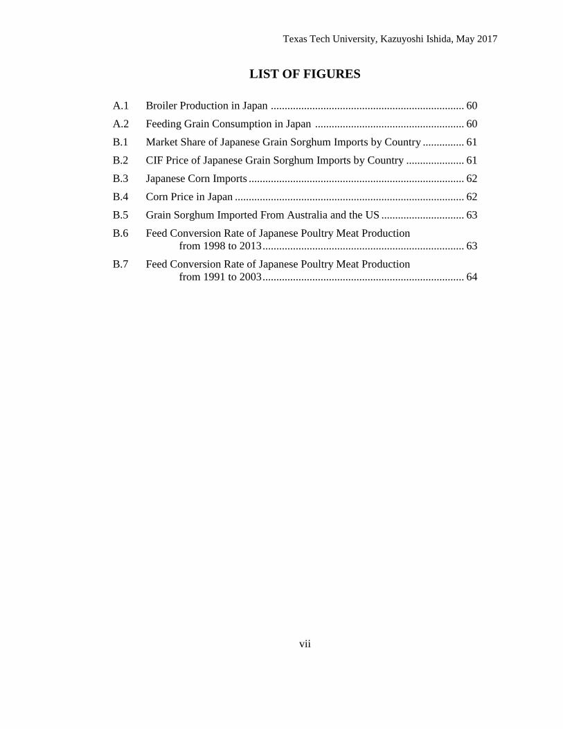
LIST OF FIGURES A.1 Broiler Production in Japan ...................................................................... 60
A.2 Feeding Grain Consumption in Japan ...................................................... 60
B.1 Market Share of Japanese Grain Sorghum Imports by Country ............... 61
B.2 CIF Price of Japanese Grain Sorghum Imports by Country ..................... 61
B.3 Japanese Corn Imports .............................................................................. 62
B.4 Corn Price in Japan ................................................................................... 62
B.5 Grain Sorghum Imported From Australia and the US .............................. 63
B.6 Feed Conversion Rate of Japanese Poultry Meat Production from 1998 to 2013 ......................................................................... 63
B.7 Feed Conversion Rate of Japanese Poultry Meat Production from 1991 to 2003 ......................................................................... 64
Texas Tech University, Kazuyoshi Ishida, May 2017
1
CHAPTER 1
AN APPROPRIATE METHODOLOGY FOR THE DEMAND ANALYSIS OF US SORGHUM IN THE JAPANESE FEEDING GRAIN MARKET
Abstract
The purpose of this paper is to identify an appropriate methodology for the
demand analysis of US grain sorghum in Japan. We have made six assumptions: 1) The
qualities of sorghum imported from different countries in Japan are not the same, 2) The
efficiency of feed in the livestock meat production has improved recently, 3) The effects
of this improved efficiency on each type of sorghum and feeding grain are not uniform, 4)
The demand for each type of feeding grain or grain sorghum has been determined by the
quantity of the final good, the production technology, and the own and the other substitute
goods prices, 5) The number of final goods using grain sorghum as an input is difficult to
be counted, and 6) The amount of feed consumption in Japanese poultry industry divided
by the quantity of its poultry meat production is used as a proxy variable for feed
efficiency. Considering these six assumptions, two models – the translog model and the
AIDS model – are appropriate for this analysis. Because a change in the consumption of
corn affects the demand for US and Australian grain sorghum differently in the Japanese
market, the separability condition between the group of sorghum imports from different
origins and other types of feeding grain may not be met. Therefore, the good’s group in
this analysis needs to include other kinds of feeding grain.
Texas Tech University, Kazuyoshi Ishida, May 2017
2
Introduction
Grain sorghum is a major feeding grain mainly used for livestock feeding.
Substitutes for grain sorghum are corn, oats, barley and other alternative grains. In Japan,
grain sorghum is used for poultry feeding, and it is imported from the US, Australia, and
Argentina. However, US grain sorghum has become less popular in the Japanese market.
One possible reason of this demand condition is that US grain sorghum is low quality,
compared to corn, or even to Australian grain sorghum. In Australia, the grain futures
market opened in 2003, and Australian grain sorghum was listed in this futures market
(Spragg, 2008). Because grain futures contracts were good tools for managing the risk of
its price volatility for Australian farmers, the traded volume of grain futures has been
increasing from the inception of this futures market (Spragg). Australian farmers who
have futures contract of grain sorghum need to deliver grain sorghum quality specified by
the Grain Trade Australia (GTA) sorghum standards (Australian Security Exchange,
2016). As a result, the quality of Australian grain sorghum has been more stable and more
reliable. On the other hand, there is no futures market for US grain sorghum. For this
reason, the quality of US grain sorghum may be still unstable and low. Thus, livestock
feeders, especially in Japan prefer corn and Australian grain sorghum for feeding grain.
However, grain sorghum production is now favorable for dryland in the
Central Plain area of the US, because its production requires less amount of water than
corn production; nowadays, the underground water in Kansas and Texas are depleting. In
order to increase US exports of grain sorghum to Japan, it is necessary to analyze its
demand in the Japanese feeding grain market. If the demand for US sorghum in Japan
Texas Tech University, Kazuyoshi Ishida, May 2017
3
expands, its total demand may increase significantly. Japan was the third largest importer
of grain sorghum, and was the second largest destination for US exports of grain sorghum
in 2014 (USDA Foreign Agriculture Service, 2016). The purpose of this dissertation is to
identify causes of the contraction of the market share of US grain sorghum in the Japanese
market.
Some researchers assume that the quality of each type of feeding grain is
uniform, and its origin does not affect its quality. Thus the Armington model, which was
developed by Armington (1969), has been used for analyzing these demands. The
assumption of this model is that the demand for a certain kind of feeding grain from some
origin is influenced only by its relative price against those of the same type of feeding
grain from other origins. The Armington model imposes strong assumptions and there is
need to examine alternative models to estimate income and price effects on the demand
for grain sorghum imported from different countries in Japan. First, we identify how the
demand for goods is affected by their quality differential, and see whether this effect has
conflict with the assumption of the Armington model. If the conflict exists, the Armington
model is not suitable for this research.
Given that grain sorghum is an input good for the production of livestock
goods, the analysis in this research is on the demand for an intermediate good. Since
efficiency of livestock feed has been improving during the last ten years in Japan, this
improvement may affect the demand for grain sorghum. Therefore, the enhancement of
livestock feed needs to be taken into consideration for the demand analysis.
Texas Tech University, Kazuyoshi Ishida, May 2017
4
For conducting demand analysis of a good from different origins, Armington
considered that every goods’ groups on the analysis were composed of the same goods
originated from different locations. It was assumed that the weak separability condition
for this good grouping was satisfied. However, in this research, if grain sorghum from a
certain country is a substitute good for other type of feeding grain, that condition may be
violated. For identifying items on the goods’ group, the weak separability condition
between the good groups of sorghum imported from different countries and other types of
feeding grains is examined
The purpose of this chapter is to identify a methodology for the demand
analysis of grain sorghum in the Japanese market, and, in the next chapter, an empirical
analysis about the loss of the market share is conducted. The chapter is composed of four
sections. In the first section, we check whether the quality differential causes a problem in
the analysis based on the Armington model. In the second section, we identify the
appropriate model for this research, and in the third section, we assess the weak
separability condition. The last section summarizes conclusions.
The Effect of Quality Differential on Demand
In this section, how the quality differential of grain sorghum imported from
different countries affects their respective demand in the Japanese market is discussed.
Next, it is explained whether the effect of this quality differential could be accommodated
into the Armington model. There are several ways for measuring the quality of sorghum
from every country. One way to do it is to run a hedonic regression, in which the price of
Texas Tech University, Kazuyoshi Ishida, May 2017
5
sorghum from different origins is regressed on its quality characteristics. The values of
quality characteristics are estimated from the parameter values of this regression, and the
quality value of these types of sorghum are calculated using the estimated values of
quality characteristics. However, it is difficult to obtain quality-related data for this
purpose. One alternative way for measuring the quality of sorghum imported from
different locations is to approximate the effect of their quality on their demand.
Cramer (1973) demonstrated the quality effect on demand by showing the
difference between income and expenditure elasticities.
𝑙𝑙𝑙𝑙 𝑥𝑥𝑖𝑖 = 𝑙𝑙𝑙𝑙 𝑝𝑝𝑖𝑖 + ln 𝑞𝑞𝑖𝑖 (1)
𝛿𝛿𝑙𝑙𝑙𝑙𝑙𝑙𝑖𝑖𝛿𝛿𝑙𝑙𝑙𝑙𝛿𝛿
= 𝛿𝛿𝑙𝑙𝑙𝑙𝑞𝑞𝑖𝑖𝛿𝛿𝑙𝑙𝑙𝑙𝛿𝛿
+ 𝛿𝛿𝑙𝑙𝑙𝑙𝑝𝑝𝑖𝑖𝛿𝛿𝑙𝑙𝑙𝑙𝛿𝛿
(2)
𝑙𝑙𝑙𝑙𝑙𝑙 = 𝑙𝑙𝑙𝑙∑𝑥𝑥𝑖𝑖 (3) Total Expenditure
In equation (1), xi is the expenditure for good i. Equation (2) is the derivative of equation
(1) with regard to income (y). The first term in the right hand side of equation (2) is
income elasticity, which is the elasticity of demand in terms of physical quantity. The
term in the left hand side of this equation is expenditure elasticity. Cramer stated that the
second term in the right hand side of the equation (2) is quality elasticity. Nelson (1991)
claimed that the use of this elasticity biases estimation, showing one example. If one buys
more Haagen-dazs ice cream and less low-quality ice cream as his or her income rises, the
income elasticity may be negative in this case. Thus, he stated that it is not appropriate to
judge that ice cream is an inferior good from this income elasticity. He concluded that an
increase on the average price of a certain group of goods purchased by consumers due to
Texas Tech University, Kazuyoshi Ishida, May 2017
6
the rise of their income, which is quality elasticity, should be taken into account for
estimating income elasticity.
Many researchers have estimated quality elasticities of goods based on this
concept. Yu and Abler (2005) estimated the quality elasticity of food consumption in eight
different regions in China. They conducted the regression of the average price of each
category of food on the average income and the values of other characteristics of
households in each region on the panel data. In this regression, the parameter of the
average household income is the quality elasticity. They concluded that the quality
elasticity of beef and sea food were high, and that of vegetables was low.
Tey et al (2008) conducted a survey of household expenditures in Malaysia,
and estimated the quality elasticity of each group of food using cross sectional data of
low- and high-income households. They performed a regression of each type of food
price on food expenditure and other relevant variables in the dataset of low-income and
high-income households, respectively. It was found out that the parameter of the food
expenditure was positively significant, and this parameter value was high in the high-
income households. Cox and Wohlgenant (1986) analyzed the cross section price
variability in food consumption in the western area of the US, and calculated the
deviations of the prices of vegetables consumed by each household from the average
prices of these goods in the area. They ran a regression of the prices on household
characteristics variables, including income and residential area characteristics.
Texas Tech University, Kazuyoshi Ishida, May 2017
7
Some researchers have a different approach for estimating quality elasticity.
Chung (2006) induced the quality elasticity from the difference between quality adjusted
price elasticity and unadjusted price elasticity.
𝑃𝑃 = 𝑝𝑝∗ ∗ 𝑃𝑃𝑃𝑃 (4)
𝑄𝑄𝑄𝑄𝑄𝑄𝑙𝑙𝑄𝑄𝑄𝑄𝑙𝑙 𝐸𝐸𝑙𝑙𝑄𝑄𝐸𝐸𝑄𝑄𝑄𝑄𝑃𝑃𝑄𝑄𝑄𝑄𝑙𝑙 = 𝛿𝛿𝛿𝛿𝛿𝛿𝛿𝛿− 𝛿𝛿𝛿𝛿
𝛿𝛿𝛿𝛿𝛿𝛿 (5)
In equation (4), P is the average price of a goods’ group, and p* is a vector of relative
prices of goods belonging to a certain goods’ group. He assumed that the relative price of
each good which is an element of a goods’ group reflects its quality, and identifies the
value of Pc in equation (4). Additionally, the derivative value of the physical quantity in
terms of Pc was calculated as quality adjusted price elasticity. Quality elasticity is found
in equation (5).
Grain sorghum quality depends on its origin. For example, the containment
level of tannin (a subsistence preventing livestock digestion) of Argentina sorghum is high
(Capehart et al, 2014). This quality differential may affect the quality elasticity of grain
sorghum produced in different places. If the demand for grain sorghum increases in Japan,
this increase would lead to the expansion of the total expenditure on grain sorghum of
Japanese livestock feeders. Since Japan is the third largest importer of grain sorghum in
the world, Japan is a price maker in its international market. Thus, this expansion of the
total expenditure may cause an increase in the average price of grain sorghum. If the
qualities of grain sorghum from all origins are the same, the price of every type of grain
sorghum should go up the same way. In this case, Japanese livestock feeders pay the
uniform price for all types of this commodity, since there is no quality differential among
Texas Tech University, Kazuyoshi Ishida, May 2017
8
them. If the qualities of grain sorghum imported from different countries are different, the
increases of their prices would not be the same. If the quality of grain sorghum from a
certain country is high, the effect of the total expenditure on the price of this type of grain
sorghum is large.
A shortage of grain sorghum supply in a country may increase the average
grain sorghum price in Japan, increasing the total sorghum expenditure. For example,
suppose a severe drought happens in Australia. The supply of grain sorghum in Australia
would decline, and this drought would raise the price of grain sorghum not only in
Australia but also in the other countries. This increased price of Australian grain sorghum
has a substitution effect on the demand for the same good from these other countries. The
total expenditure on grain sorghum would increase in Japan, because the price elasticity of
sorghum demand might be inelastic. In this case, if the qualities of grain sorghum
produced in all countries are different, the increases of their prices are not the same.
Therefore, the origin of sorghum may affect its quality elasticity, and equation (2) is
appropriate for estimations of the demands for grain sorghum from different origins in
Japan
ln(wi) = 𝛼𝛼𝑖𝑖 ∗ ( 𝑙𝑙𝑙𝑙𝛿𝛿𝑖𝑖∑𝑤𝑤𝑗𝑗𝑙𝑙𝑙𝑙𝛿𝛿𝑗𝑗
) (6)
Equation (6) is the model developed by Armington. The variable wi in this
equation is the expenditure share of good i. Equation (6) does not have the variable of the
total expenditure. The Armington model assumes that the effects of this expenditure
change on the demands for goods are the same, and that this change does not alter the
Texas Tech University, Kazuyoshi Ishida, May 2017
9
expenditure share of each good. As a result, the variable of the total expenditure is omitted
in this model.
If the demand for grain sorghum from each origin has a different quality
elasticity, the Armington model may not be fitted for this analysis. Since the variable of
the total expenditure is missed in the Armington model (equation 6), the effects of the
total expenditure on the expenditure of each good is homothetic. Therefore, the impacts of
the total expenditure on both the consumption quantity and the price of each good are also
homothetic. Hence, the Armington model cannot accommodate the effect of quality
differential on the demands, and this model cannot be chosen for the analysis of this
paper.
Identification of Appropriate Models
Because the Armington model was rejected, other models need to be used for
the demand analysis of grain sorghum. For finding out appropriate models for this
analysis, the following assumptions about Japanese demand for feeding grain are taken
into consideration.
1) The budget for feeding grain may influence feeding grain prices (quality effect),
2) The efficiency of feed has been improving in Japan,
3) The effects of this improved efficiency on the demands for grain sorghum from
different origins and different types of feeding grain are not the same,
Texas Tech University, Kazuyoshi Ishida, May 2017
10
4) The demand for each type of feeding grain or grain sorghum has been determined
by the quantity of the final good, the production technology, and the own and the
other substitute goods prices,
5) The number of final goods using grain sorghum as an input is difficult to count,
and
6) The amount of the feed consumption of Japanese poultry feeding divided by the
quantity of its poultry meat production is used for an approximate variable of the
feed efficiency.
Willems, Miller and Wood (2013) stated that the feed efficiency in the poultry
industry in the world has improved from 2008 to 2013, and this improvement is partly due
to an increase in the price of feeding grain worldwide. They conclude that this price
increase raised poultry production costs, and encouraged livestock feeders to improve feed
efficiency of their poultry production. There are three ways to improve feed efficiency.
The first one is enhancement in poultry production management, such as optimizing
temperatures (Havenstein et al, 2003). The second one is improvement in the formulation
of poultry feed (Havenstein et al, 2003). The last one is a genetic selection by choosing
birds with better-feed efficiency for poultry production (Willems, Miller and Wood).
Willems, Miller, and Wood stated that poultry nutrition research had found out precise
formulations of poultry feed, and that these formulations supplied an appropriation ratio of
nutrition for birds in order that they take a necessary amount of feeding grain.
In Japan, most of poultry feed is formula feed. Formula feed was developed
by blending nutrition components with scientific knowledge before mid-1980 (Lin et al.,
Texas Tech University, Kazuyoshi Ishida, May 2017
11
1990). The Japanese Ministry of Agriculture, Forestry, and Fishery has encouraged
improving efficiency of poultry formula corresponding to the recent increase in the price
of feeding grain (Yamauchi, 2014). Thus, Japanese feed companies have improved
formulations of formula feed so that smaller amounts of this feed is needed for poultry to
obtain specific nutrients (Yamauchi, 2014). Figure 1 in the Appendix shows the increase
of the broiler production during the past 10 years in Japan, and Figure 2 illustrates the
decrease of the feeding grain consumption over the same time. From these two figures, it
can be seen that the feed conversion rate has improved in Japanese broiler production.
Therefore, assumption (1) needs to be taken into account.
Forty-three percent of formula feed content is corn, and grain sorghum
represents seven percent (Yamauchi, 2014). Grain sorghum is a substitute input to corn for
this feed, since these two types of feeding grain are primary used for providing energy to
poultry. However, grain sorghum has the substance named tannin, which affects poultry
digestion; other types of feeding grain do not have this substance (Selle, Cadogan, and
Bryden, 2010). Rodoriguez (2007) reported that the tannin level of grain sorghum is
positively correlated with the depression of feed efficiency and body weight gain of
poultry. Australian and US grain sorghum have low levels of tannin, which is less than
1%; on the other hand, Argentina sorghum contains more than 5% level of tannin. Selle,
Cardogan, and Bryden found out that low-levels tannin grain sorghum may be acceptable
for poultry feedstuff (corn is still preferable). However, they also found out that a poultry
ration based on grain sorghum has another problem. They stated that the texture and
physical property of grain sorghum affect the amino acid digestibility of poultry, influence
Texas Tech University, Kazuyoshi Ishida, May 2017
12
the growth performance, and that these characteristics of grain sorghum have high
variability. Therefore, it is concluded that the poultry feed based on grain sorghum may
cause inconsistent poultry growth. The texture and physical property of Australian grain
sorghum might have small variation, since its futures market set the standards of these
characteristics. Hence, more amount of Australian sorghum and corn and less amount of
Argentina and US sorghum might have been used for the production of formula feed in
Japan for its improvement of feed conversion ratio. Therefore, the effects of an
improvement of poultry feed efficiency on the demand for each type of feeding grain
might be different, and assumption (2) needs to be considered.
Usually, Japanese livestock feeders decide the total heads of their livestock
based on the price of each category of input goods (for example, feeding grain, water, and
labor) in the previous period. After this decision is made, the amount of each type of
feeding grain or grain sorghum from different origin is determined. Therefore, every type
of feeding grain may be affected by the quantity of the final goods, the own and other
input goods’ prices, and the efficiency improvement of feed.
It is not easy to count the number of final goods using grain sorghum as an
input. Grain sorghum is fed to cattle, poultry, and pork. Cattle produces meat, milk, and
skin; and poultry provides meat and eggs for human consumption. Therefore, many kinds
of goods take grain sorghum as an input good. Simple counting of these final goods may
not be appropriate since the importance of grain sorghum as an input good is different for
each of the final goods. Since identifying the weight reflecting the importance of each of
the final goods is not feasible, weight-counting of the final goods is impossible. Hence,
Texas Tech University, Kazuyoshi Ishida, May 2017
13
the quantity of the final goods cannot be measured. The conditional input factor model,
which takes the variables of the own and other input goods’ price, and the quantity of final
goods, is derived from the profit function of production. Arzac and Wilkinson (1979) used
this model for analyzing the demand for corn in the US. However, it is not appropriate for
our analysis since the quantity of final goods cannot be counted.
It is impossible to find out the variable of the exact feed efficiency of Japanese
livestock feeding, since the quantity of the final product using feeding grain as an input
good cannot be measured. Therefore, an approximate variable of the feed efficiency is
used as its indicator. Since the largest portion of grain sorghum is used for poultry feeding
in Japan, the production quantity of poultry meat divided by its feeding consumption
quantity might be a best indicator of the feed efficiency in this demand analysis.
Based on the assumptions from (1) to (6), the model derived from the translog
cost function might be appropriate. The translog cost function is a flexible functional
form. Since it is difficult to be identified how to specify the production or cost function of
livestock feeding in Japan, it is appropriate to use this flexible cost function. The translog
cost function is given by
ln(𝐶𝐶) = 𝛼𝛼𝑜𝑜 + 𝛼𝛼𝑞𝑞 ∗ ln(𝑄𝑄) + 𝛼𝛼𝐴𝐴 ∗ ln(𝐴𝐴) + ∑ 𝛽𝛽𝑖𝑖 ∗ ln(𝑝𝑝𝑖𝑖)𝑖𝑖 + ∑ ∑ βijln(𝑝𝑝𝑗𝑗)𝑗𝑗 ∗ ln(𝑝𝑝𝑖𝑖)𝑖𝑖
+∑ βiQ ∗ ln (𝑝𝑝𝑖𝑖)𝑖𝑖 ∗ ln(𝑄𝑄) + ∑ βiA ∗ ln(𝑝𝑝𝑖𝑖)𝑖𝑖 ∗ ln(𝐴𝐴) + ∑ βQQ ∗ ln(𝑄𝑄)𝑖𝑖2
+ ∑ βAA ∗ ln(𝐴𝐴)𝑖𝑖2 + ∑ βQAln (Q) ∗ ln(𝐴𝐴)𝑖𝑖 (7)
The variables A and Q indicate technology and the quantity of final products,
respectively. Yuhn (1991) derived an indirect production function from equation (7).
Texas Tech University, Kazuyoshi Ishida, May 2017
14
ln(𝑄𝑄) = 𝛾𝛾𝑜𝑜 + 𝛾𝛾𝛿𝛿 ∗ ln(𝐶𝐶) + 𝛾𝛾𝐴𝐴 ∗ ln(𝐴𝐴) + ∑ 𝛾𝛾𝑖𝑖 ∗ ln(𝑝𝑝𝑖𝑖)𝑖𝑖 + ∑ ∑ γijln(𝑝𝑝𝑗𝑗)𝑗𝑗 ∗ ln(𝑝𝑝𝑖𝑖)𝑖𝑖
+∑ γiQ ∗ ln (𝑝𝑝𝑖𝑖)𝑖𝑖 ∗ ln(𝐶𝐶) + ∑ γiA ∗ ln(𝑝𝑝𝑖𝑖)𝑖𝑖 ∗ ln(𝐴𝐴) + ∑ γQQ ∗ ln(𝐶𝐶)𝑖𝑖2
+ ∑ γ ∗ ln(𝐴𝐴)𝑖𝑖2 + ∑ γQAln (C) ∗ ln(𝐴𝐴)𝑖𝑖 (8)
Equation (8) is the derived indirect production function. Yuhn derived the
equation of the expenditure share of the good i from equation (8) by using the Roy’s
identity.
𝑤𝑤𝑖𝑖 = − 𝛾𝛾𝑖𝑖+𝛾𝛾𝑖𝑖𝑖𝑖∗ln(𝐶𝐶)+∑ 𝛾𝛾𝑖𝑖𝑗𝑗𝑗𝑗 ln𝑝𝑝𝑗𝑗+𝛾𝛾𝑖𝑖𝑖𝑖 ln(𝐴𝐴)
𝛾𝛾𝑖𝑖+𝛾𝛾𝑖𝑖𝑖𝑖∗ln(𝐶𝐶)+∑ 𝛾𝛾𝑗𝑗𝑗𝑗𝑗𝑗 ln𝑝𝑝𝑗𝑗+𝛾𝛾𝑗𝑗𝑖𝑖 ln(𝐴𝐴) (9)
Equation (9) is the derived expenditure share equation. The price and income
elasticity of good i can be estimated in equation (9). In this equation, the expenditure share
of the good i is affected by the technology improvement, and therefore, the assumptions
(2) and (3) are considered.
The existence of quality elasticity has no conflict with equation (9). The
elasticity of the expenditure of good i with the total budget in equation (9) is equation
(10).1
𝛿𝛿𝑙𝑙𝑙𝑙𝛿𝛿𝑖𝑖𝛿𝛿𝑙𝑙𝑙𝑙𝐶𝐶
=
1 − 𝛾𝛾𝑖𝑖𝑖𝑖∗(𝛾𝛾𝑖𝑖+𝛾𝛾𝑖𝑖𝑖𝑖∗ln(𝐶𝐶)+∑ 𝛾𝛾𝑗𝑗𝑗𝑗𝑗𝑗 ln𝑝𝑝𝑗𝑗+𝛾𝛾𝑗𝑗𝑖𝑖 ln(𝐴𝐴))−𝛾𝛾𝑖𝑖𝑖𝑖∗(𝛾𝛾𝑖𝑖+𝛾𝛾𝑖𝑖𝑖𝑖∗ln(𝐶𝐶)+∑ 𝛾𝛾𝑖𝑖𝑗𝑗𝑗𝑗 ln𝑝𝑝𝑗𝑗+𝛾𝛾𝑖𝑖𝑖𝑖 ln(𝐴𝐴))(𝛾𝛾𝑖𝑖+𝛾𝛾𝑖𝑖𝑖𝑖∗ln(𝐶𝐶)+∑ 𝛾𝛾𝑗𝑗𝑗𝑗𝑗𝑗 ln𝑝𝑝𝑗𝑗+𝛾𝛾𝑗𝑗𝑖𝑖 ln(𝐴𝐴))2∗𝑆𝑆𝑖𝑖
(10)
1 δSi𝛿𝛿 ln𝐶𝐶
= 𝛿𝛿𝑆𝑆𝑖𝑖𝛿𝛿𝐶𝐶∗ 𝐶𝐶 = 𝛿𝛿𝛿𝛿𝑖𝑖
𝛿𝛿𝐶𝐶− 𝐸𝐸𝑖𝑖 ∗ 𝐶𝐶−1 Therefore, δSi
𝛿𝛿 ln𝐶𝐶 ∗ 𝐶𝐶𝛿𝛿𝑖𝑖
+ 1 = 𝛿𝛿𝑙𝑙𝑙𝑙𝛿𝛿𝑖𝑖𝛿𝛿𝑙𝑙𝑙𝑙𝐶𝐶
Texas Tech University, Kazuyoshi Ishida, May 2017
15
Equation (9) has no conflict with the existence of the quality effect. Unless the
second term of the right-hand side of equation (10) is one, the elasticity of this
expenditure of good i with the total budget is not zero in equation (10). The quality
elasticity of good i can be the difference between this expenditure elasticity and the
expenditure elasticity of the demand for good i (the last term of the right hand side of
equation 2).
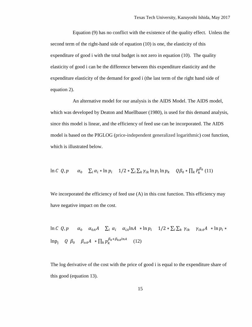
An alternative model for our analysis is the AIDS Model. The AIDS model,
which was developed by Deaton and Muellbauer (1980), is used for this demand analysis,
since this model is linear, and the efficiency of feed use can be incorporated. The AIDS
model is based on the PIGLOG (price-independent generalized logarithmic) cost function,
which is illustrated below.
ln𝐶𝐶(𝑄𝑄,𝑝𝑝) = 𝛼𝛼0 + ∑ 𝛼𝛼𝑖𝑖 ∗ ln 𝑝𝑝𝑖𝑖 + 1/2 ∗ ∑ ∑ 𝛾𝛾𝑖𝑖𝑖𝑖 ln 𝑝𝑝𝑖𝑖 ln𝑝𝑝𝑖𝑖𝑖𝑖𝑖𝑖𝑖𝑖 + 𝑄𝑄𝛽𝛽0 ∗ ∏ 𝑃𝑃𝑖𝑖𝛽𝛽𝑘𝑘
𝑖𝑖 (11)
We incorporated the efficiency of feed use (A) in this cost function. This efficiency may
have negative impact on the cost.
ln𝐶𝐶(𝑄𝑄,𝑝𝑝) = 𝛼𝛼0 + 𝛼𝛼0𝐴𝐴𝐴𝐴 + ∑ (𝛼𝛼𝑖𝑖 + 𝛼𝛼𝑖𝑖𝐴𝐴ln𝐴𝐴) ∗ ln 𝑝𝑝𝑖𝑖 + 1/2 ∗ ∑ ∑ (𝛾𝛾𝑖𝑖𝑖𝑖 + 𝛾𝛾𝑖𝑖𝑖𝑖𝐴𝐴𝐴𝐴) ∗𝑖𝑖𝑖𝑖𝑖𝑖 ln𝑝𝑝𝑖𝑖 ∗
lnpj + 𝑄𝑄(𝛽𝛽0 + 𝛽𝛽𝑜𝑜𝐴𝐴𝐴𝐴) ∗ ∏ 𝑝𝑝𝑖𝑖𝛽𝛽𝑘𝑘+𝛽𝛽𝑘𝑘𝑘𝑘𝑙𝑙𝑙𝑙𝐴𝐴
𝑖𝑖 (12)
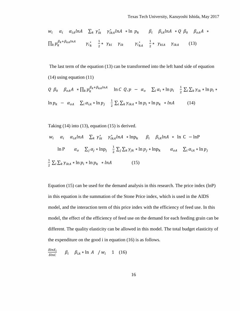
The log derivative of the cost with the price of good i is equal to the expenditure share of
this good (equation 13).
Texas Tech University, Kazuyoshi Ishida, May 2017
16
𝑤𝑤𝑖𝑖 = 𝛼𝛼𝑖𝑖 + 𝛼𝛼𝑖𝑖𝐴𝐴𝑙𝑙𝑙𝑙𝐴𝐴 + ∑ (𝛾𝛾𝑖𝑖𝑖𝑖∗ + 𝛾𝛾𝑖𝑖𝑖𝑖𝐴𝐴∗ 𝑙𝑙𝑙𝑙𝐴𝐴) ∗ ln (𝑝𝑝𝑖𝑖)𝑖𝑖 + (𝛽𝛽𝑖𝑖 + 𝛽𝛽𝑖𝑖𝐴𝐴𝑙𝑙𝑙𝑙𝐴𝐴) ∗ 𝑄𝑄(𝛽𝛽0 + 𝛽𝛽𝑜𝑜𝐴𝐴𝐴𝐴) ∗
∏ 𝑝𝑝𝑖𝑖𝛽𝛽𝑘𝑘+𝛽𝛽𝑘𝑘𝑘𝑘𝑙𝑙𝑙𝑙𝐴𝐴
𝑖𝑖 𝛾𝛾𝑖𝑖𝑖𝑖∗ = 1
2∗ (𝛾𝛾𝑖𝑖𝑖𝑖 + 𝛾𝛾𝑖𝑖𝑖𝑖) 𝛾𝛾𝑖𝑖𝑖𝑖𝐴𝐴
∗ = 12∗ (𝛾𝛾𝑖𝑖𝑖𝑖𝐴𝐴 + 𝛾𝛾𝑖𝑖𝑖𝑖𝐴𝐴) (13)
The last term of the equation (13) can be transformed into the left hand side of equation
(14) using equation (11)
𝑄𝑄(𝛽𝛽0 + 𝛽𝛽𝑜𝑜𝐴𝐴𝐴𝐴) ∗ ∏ 𝑝𝑝𝑖𝑖𝛽𝛽𝑘𝑘+𝛽𝛽𝑘𝑘𝑘𝑘𝑙𝑙𝑙𝑙𝐴𝐴
𝑖𝑖 = ln𝐶𝐶(𝑄𝑄,𝑝𝑝) − (𝛼𝛼𝑜𝑜 + ∑ 𝛼𝛼𝑖𝑖 ∗ ln 𝑝𝑝𝑖𝑖𝑖𝑖 + 12
∑ ∑ 𝛾𝛾𝑖𝑖𝑖𝑖 ∗ ln𝑝𝑝𝑖𝑖 ∗𝑖𝑖𝑖𝑖
ln 𝑝𝑝𝑖𝑖) − (𝛼𝛼𝑜𝑜𝐴𝐴 + ∑ 𝛼𝛼𝑖𝑖𝐴𝐴 ∗ ln 𝑝𝑝𝑗𝑗𝑖𝑖 + 12
∑ ∑ 𝛾𝛾𝑖𝑖𝑖𝑖𝐴𝐴 ∗ ln𝑝𝑝𝑖𝑖 ∗ ln 𝑝𝑝𝑖𝑖) ∗ 𝑙𝑙𝑙𝑙𝐴𝐴𝑖𝑖𝑖𝑖 (14)
Taking (14) into (13), equation (15) is derived.
𝑤𝑤𝑖𝑖 = 𝛼𝛼𝑖𝑖 + 𝛼𝛼𝑖𝑖𝐴𝐴𝑙𝑙𝑙𝑙𝐴𝐴 + ∑ (𝛾𝛾𝑖𝑖𝑖𝑖∗ + 𝛾𝛾𝑖𝑖𝑖𝑖𝐴𝐴∗ 𝑙𝑙𝑙𝑙𝐴𝐴) ∗ lnpk𝑖𝑖 + (𝛽𝛽𝑖𝑖 + 𝛽𝛽𝑖𝑖𝐴𝐴𝑙𝑙𝑙𝑙𝐴𝐴) ∗ (ln(C) − lnP)
ln P = (𝛼𝛼𝑜𝑜 + ∑ 𝛼𝛼𝑗𝑗 ∗ lnpj𝑗𝑗 + 12
∑ ∑ 𝛾𝛾𝑗𝑗𝑖𝑖 ∗ ln 𝑝𝑝𝑗𝑗 ∗ lnpk) + (𝛼𝛼𝑜𝑜𝐴𝐴 + ∑ 𝛼𝛼𝑖𝑖𝐴𝐴 ∗ ln 𝑝𝑝𝑗𝑗𝑖𝑖 +𝑖𝑖𝑗𝑗
12
∑ ∑ 𝛾𝛾𝑖𝑖𝑖𝑖𝐴𝐴 ∗ ln 𝑝𝑝𝑖𝑖 ∗ ln 𝑝𝑝𝑖𝑖) ∗ 𝑙𝑙𝑙𝑙𝐴𝐴𝑖𝑖𝑖𝑖 (15)
Equation (15) can be used for the demand analysis in this research. The price index (lnP)
in this equation is the summation of the Stone Price index, which is used in the AIDS
model, and the interaction term of this price index with the efficiency of feed use. In this
model, the effect of the efficiency of feed use on the demand for each feeding grain can be
different. The quality elasticity can be allowed in this model. The total budget elasticity of
the expenditure on the good i in equation (16) is as follows.
𝛿𝛿𝑙𝑙𝑙𝑙𝛿𝛿𝑖𝑖𝛿𝛿𝑙𝑙𝑙𝑙𝐶𝐶
= (𝛽𝛽𝑖𝑖 + 𝛽𝛽𝑖𝑖𝐴𝐴 ∗ ln(𝐴𝐴))/ 𝑤𝑤𝑖𝑖 + 1 (16)
Texas Tech University, Kazuyoshi Ishida, May 2017
17
Unless the first term in the right hand side of equation (16) is negative one, the value of
this derivative is nonzero. Like equation (9), the existence of quality elasticity does not
have a conflict
It is difficult to compare model (15) with model (9) in terms of appropriateness
for this demand analysis ex ante, if the regression of model (9) can estimate its parameter.
After running the regressions of these two models, the AICs and SICs of these two
regressions need to be checked.
Separability Condition
For analyzing the demand for US grain sorghum in Japan, we need to identify
items on the goods’ group on this analysis. According to the Armington’s assumption, US
sorghum is included in the goods’ group which is composed of sorghum from different
countries. However, if grain sorghum from at least one origin is a complement or
substitute good for other types of feeding grain, these types of feeing grain needed to be
included in the good group on the research. Therefore, this Armington assumption may
not be valid for this research.
Japanese livestock feeders allocate their purchase of capital, labor, feeding
grain and other intermediate goods for maximizing the profit of their production. As
mentioned earlier, at first, they decide the optimal livestock meat production quantity
based on their expected market price of livestock meats and the prices of the input goods.
Therefore, the demands for those goods depend on the quantity of livestock meat. Since it
Texas Tech University, Kazuyoshi Ishida, May 2017
18
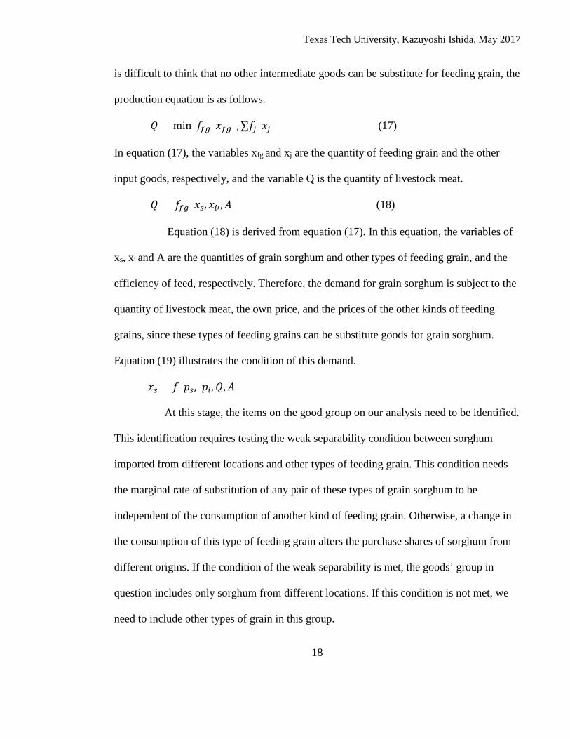
is difficult to think that no other intermediate goods can be substitute for feeding grain, the
production equation is as follows.
𝑄𝑄 = min (𝑓𝑓𝑓𝑓𝑓𝑓(𝑥𝑥𝑓𝑓𝑓𝑓),∑𝑓𝑓𝑗𝑗(𝑥𝑥𝑗𝑗)) (17)
In equation (17), the variables xfg and xj are the quantity of feeding grain and the other
input goods, respectively, and the variable Q is the quantity of livestock meat.
𝑄𝑄 = 𝑓𝑓𝑓𝑓𝑓𝑓(𝑥𝑥𝑠𝑠, 𝑥𝑥𝑖𝑖′,𝐴𝐴) (18)
Equation (18) is derived from equation (17). In this equation, the variables of
xs, xi and A are the quantities of grain sorghum and other types of feeding grain, and the
efficiency of feed, respectively. Therefore, the demand for grain sorghum is subject to the
quantity of livestock meat, the own price, and the prices of the other kinds of feeding
grains, since these types of feeding grains can be substitute goods for grain sorghum.
Equation (19) illustrates the condition of this demand.
𝑥𝑥𝑠𝑠 = 𝑓𝑓 (𝑝𝑝𝑠𝑠, 𝑝𝑝𝑖𝑖,𝑄𝑄,𝐴𝐴)
At this stage, the items on the good group on our analysis need to be identified.
This identification requires testing the weak separability condition between sorghum
imported from different locations and other types of feeding grain. This condition needs
the marginal rate of substitution of any pair of these types of grain sorghum to be
independent of the consumption of another kind of feeding grain. Otherwise, a change in
the consumption of this type of feeding grain alters the purchase shares of sorghum from
different origins. If the condition of the weak separability is met, the goods’ group in
question includes only sorghum from different locations. If this condition is not met, we
need to include other types of grain in this group.
Texas Tech University, Kazuyoshi Ishida, May 2017
19
The necessary and sufficient condition for this weak separability condition
proposed by Goldman and Uzawa (1964) is condition (20).
𝑆𝑆𝑖𝑖𝑗𝑗 = 𝜃𝜃𝑟𝑟𝑗𝑗 ∗𝛿𝛿𝑙𝑙𝑖𝑖𝛿𝛿𝛿𝛿∗ 𝛿𝛿𝑙𝑙𝑗𝑗𝛿𝛿𝛿𝛿
∀ 𝑄𝑄 ∈ 𝑟𝑟 (20)
Sij is the compensated substitution effect between sorghum from a particular origin (i) and
each type of feeding grain except sorghum (j). The goods’ group r is composed of
sorghum imported from any country to Japan. ϴrj is the degree of the substitutability
between sorghum and other types of feeding grains. Equation (21) is derived from
equation (20).
𝑆𝑆𝑘𝑘𝑗𝑗𝛿𝛿𝑥𝑥𝑘𝑘𝛿𝛿𝛿𝛿
= 𝑆𝑆𝑖𝑖𝑗𝑗𝛿𝛿𝑥𝑥𝑖𝑖𝛿𝛿𝛿𝛿
∀ 𝑄𝑄,𝑘𝑘 ∈ 𝑟𝑟 (21)
In equation (21), goods k and i belong to the grain sorghum group. If this equation holds,
the sufficient and necessary condition of the weak separability (condition [20]) is met.
As mentioned earlier, Australian grain sorghum became an input for formula
feed due to its stable quality. This trend may strengthen the degree of the substitution
between Australian grain sorghum and corn in the Japanese feeding grain market.
Therefore, the degree of the substitution between corn and Australian grain sorghum may
be different from that between US sorghum and corn, and condition (20) may be not met.
In case the weak separability condition is not satisfied, corn and other kinds of feeding
grain need to be included in the goods group of this question.
Conclusion
Taking into account quality effects of grain sorghum from different origins on
their demand, we judged that the Armington model is not appropriate for the analysis of
Texas Tech University, Kazuyoshi Ishida, May 2017
20
the demand for grain sorghum in the Japanese feeding grain market. The assumption of
this model does not take into account the quality effects. Therefore, other models are used
for the demand analysis of grain sorghum. On the other hand, given that the improvement
of feed efficiency influences the demand for each type of feeding grain in Japan, the
translog and the AIDS model, which can take the feed efficiency variable, are appropriate.
However, the variable measuring the feed efficiency of livestock feeding in Japan in these
two models is only approximated. Identification of the effect of the efficiency
improvement on the demand for US grain sorghum is important for finding out the cause
of the declining market share of US sorghum in the Japanese market. In the next chapter,
we run the regressions of these two models on the relevant data. The results of the translog
and AIDS models will and compared, using AICs (Akaike Information Criterion) in order
to find out which model is best for this demand analysis.
The separability condition between grain sorghum goods’ group, which is
composed of this commodity from different countries in Japan, and other kinds of feeding
grains may not be satisfied. Therefore, corn and other types of feeding grain might need to
be included in the goods’ group for the demand analysis of grain sorghum in Japan. In the
next chapter, we will also check this weak separability condition. We will find out the
quality elasticities of grain sorghum from different origins will be estimated based on
equation (2), and then we will examine whether these quality elasticities are not uniform.
Texas Tech University, Kazuyoshi Ishida, May 2017
21
CHAPTER 2
WHY THE MARKET SHARE OF US GRAIN SORGHUM HAS DECLINED IN THE JAPANESE MARKET?
Abstract
The market share of US grain sorghum has decreased in the Japanese market
for the last 20 years, and Australian grain sorghum has claimed the top market share. After
2008, the feed efficiency has improved in Japanese livestock feeding, and this
improvement may have affected the demand for US grain sorghum in that market. The
decline in the use of US grain sorghum may be explained by feeders avoiding US grain
sorghum because of its unstable quality. For identifying causes of the decline of the
market share of US grain sorghum, we estimated the price, expenditure and feed
efficiency (the feed conversion rate of poultry meat production) elasticities of the US and
Australian grain sorghum. The results of the analysis suggest that a change in corn price
may have positive impact on the demand for Australian grain sorghum, and may have
small effect on the demand for US grain sorghum. The recent increase in corn price might
have caused the US grain sorghum market share decline. The result of this analysis using
a Bayesian SUR indicate that the effect of the feed efficiency improvement on the own
price elasticity of US grain sorghum might become bigger from 2008 to 2013.
Texas Tech University, Kazuyoshi Ishida, May 2017
22
Introduction
Grain sorghum is mainly used for live feeding, and is a considerably good
substitute for corn. However, livestock feeders perceive that grain sorghum is inferior to
corn due to its quality. Japan produces little grain sorghum because their productivity of
grain sorghum is relatively low compared to other countries and other crops in Japan.
Nevertheless, Japan imports large volumes of grain sorghum due to the existence of a
somewhat substantial poultry livestock industry2. The United States produces and exports
a large amount of grain sorghum, mainly because its productivity of the grain is high
compared to other countries. Therefore, prices of US grain sorghum have been relatively
low in world markets allowing the US to maintain a significant market share in
international markets for long time. However, recently, the US market share has been
declining in the in foreign markets, including Japan. Figure 1 shows that the United States
held the largest share in the Japanese grain sorghum market for 20 years. However, in
recent years, Australia’s share of the same market has been constantly growing and has
now claimed the top position.
As illustrated in figure 2, the price difference between US and Australian grain
sorghum has changed a little during the past 20 years. From 1986 to 2009, US grain
sorghum was cheaper than Australian grain sorghum in the Japanese market. However,
since 2009, the former has been a little bit more expensive than the latter in Japan. If the
quality differential of these two types of grain sorghum is extremely small, they should be
almost a perfect substitute good for each other. Therefore, the small change in the price
2 The size of the livestock production in Japan (1,305 tons) is much less than that production in United States (10,568 tons), but is nearly equal to that production in Mexico (1,270 tons) in 2013
Texas Tech University, Kazuyoshi Ishida, May 2017
23
difference between US and Australian grain sorghum may flip over their market positions
in Japan. If the following hypotheses is true, this slight weakening of the price
competiveness of US grain sorghum may lead to the declining of its market share in the
Japanese market:
The cross price elasticity of Australian grain sorghum with respect to US grain
sorghum is positive and elastic.
The prices of both US and Australian grain sorghum were on the upward trend from 1998
to 2013. If this cross price elasticity is not positive, this upward trend of US grain
sorghum price might not have expanded the demand for Australian grain sorghum in the
Japanese market. In this case, this increase in US grain sorghum price may not be a cause
of the loss of its market share in the Japanese market.
There might be other causes why US grain sorghum has been losing its market
share in the Japanese market. For example, Australian grain sorghum may have become
more substitutable for corn in Japan after the opening of its futures market. As explained
in the first chapter introduction, Australian farmers have controlled the risk of the grain
sorghum price volatility by using its futures contracts. These contracts require a delivery
of grain sorghum quality specified by the futures market. As a result, the quality of
Australian grain sorghum became more reliable and more substitutable for corn than US
grain sorghum, which does not have its futures market. The recent increase in the corn
price may expand the demand for Australian grain sorghum more than that for US grain
sorghum. If the hypotheses presented below is true, the stronger substitutability of
Texas Tech University, Kazuyoshi Ishida, May 2017
24
Australian grain sorghum with corn may be a factor of the contraction of the market share
of US grain sorghum in the Japanese market:
The cross price elasticity of Australian grain sorghum with respect to corn is
larger than that of US grain sorghum.
Improvements of formulations of formula feed may also increase the demand for
Australian grain sorghum, but decrease the demand for US grain sorghum (This detail
explanation is described in the first chapter). If the following hypotheses are met, the
improvement of feed efficiency may have negative effect on the market share of US grain
sorghum in the Japanese market:
The effect of feed efficiency improvement on the demand for US grain
sorghum is negative, and
The effect of feed efficiency improvement on the demand for Australian grain
sorghum is positive
This paper investigates potential causes of the decline US grain sorghum
market share in the Japanese market by testing the four hypotheses listed. The paper is
composed of five sections. 1) Literature Review, 2) Conceptual Framework, 3) Empirical
Framework, 4) Results, and 5) Conclusion. In this empirical analysis, we checked the
quality elasticity of grain sorghum imported from each country, which is the derivative of
each respective price with the total expenditure. The purpose of this examination is
whether there are quality differentials among grain sorghum from each origin.
Texas Tech University, Kazuyoshi Ishida, May 2017
25
Literature Review
There is no study investigating the demand analysis of grain sorghum imported
from different countries into a specific country or even into the world market. However,
several previous studies have estimated price and income elasticities of similar
agricultural commodities (like rice, wheat and lumber) imported from different countries
into the markets of certain countries or the world market. As stated in the first chapter,
the Armington model has been used for the demand analysis of imported agricultural
commodities. This model has two stages. The first stage determines the quantity of each
agricultural commodity maximizing utility, and the second stage decides the quantity of
commodity from each supplier in order to minimize the expenditure. The price elasticity
of a good from each supplier is estimated from the second stage. Since this model is
based on the constant elasticity utility principle, homotheticity and single price elasticity
are assumed. Homma and Heady (1984) estimated the price elasticity of imported wheat
in several countries using the Armington model. Ito, Chen and Peterson (1986) modified
the Armington model and allowed non-homotheticity and different price elasticity for
each good in the group. Based on this modified model, they estimated the price and
expenditure elasticity of exported rice from each country in the world market. In addition,
they tested the appropriateness of the homotheticity and the single price elasticity
assumptions in the restricted model, and rejected it.
Alston, Carter and Green (1990) modified the model the same way. While Ito,
Chen, and Peterson neglected the cross price elasticity of products from different
countries, Alston, Carter, and Green added it into their modified model. They estimated
Texas Tech University, Kazuyoshi Ishida, May 2017
26
the cross price elasticity of wheat from different countries in five major importing
countries and the cross price elasticity of the cotton from different origins in these
countries.
Davis and Jasen (1994) used the Marshallian demand model derived from the
translog cost function model developed by Yuhn (1992) to estimate price and income
elasticity of lumber imported from different countries into the Japanese market. In their
research, lumber was treated as an input good. Richards et al (1997) used the AIDS model
to identify the effect of the promotion of US apple on its demand in the apple market of
Singapore and the UK. In these previous two researches, the two-stage demand model
was still assumed. The good’s group in the second stage was composed of the same goods
imported from different countries. but the demand models were not based on the CES
utility function.
Conceptual Framework
This research follows the concepts of the analyses conducted by Davis and
Jasen, and Richards et al. As is proposed by Davis and Jasen, the equation in the first stage
is a profit maximization problem. Japanese livestock feeders initially allocate their
purchase of capital, labor and intermediate goods for maximizing the profit of their
livestock production. The second stage in this analysis is not based on the constant
elasticity utility principle either. However, the good’s group in this second stage includes not
only grain sorghum imports from different countries, but also other types of feeding grain.
Texas Tech University, Kazuyoshi Ishida, May 2017
27
The profit maximization problem is equation (1).
max𝑞𝑞
π = p ∗ q(x, p) −w′x − fc (1)
δπδp
= q∗ (2)
q∗ = ffgxfgi∗ , Afg (3)
In equation (1), inputs of the livestock production, which includes feeding
grain, are x, and the prices of the inputs are w. The optimal output quantity (q) can be
determined by the Hoteling Lemma (equation (2)). Equation (3) shows the relation
between the optimal input of feeding grain and the optimal output quantity. In this
equation, the variables of xfgi and Afg are each type of feeding grain, and the feed
conversion ratio. Willems, Miller and Wood (2013) stated the feed conversion ratio of
poultry in Japan, which is the ratio of the input quantity of feeding grain to the output
weight of poultry meat, has improved for the last 10 years due to the upward trend of
prices of feeding grain worldwide. An improved formulation of formula feeds3, which is
mostly used for poultry feeding in Japan, may enhance this ratio (Yamauchi, 2014). The
effect of this improvement on each type of feeding grain may be different, and therefore,
this efficiency needed to be included.
Since Japanese livestock feeders buy each type of feeding grain to minimize
the cost of their livestock production, the equation of demand for each of these goods
3 Formula feed is made from blending feeding grain (corn, sorghum, and soybeans) based on formulation developed by nutritionist, and have every required nutrition element for livestock
Texas Tech University, Kazuyoshi Ishida, May 2017
28
(equation [4-1]) is derived from the minimizing input cost of feeding grain for this
production (equation [4]).
Min pfgi′ xfgi 𝐸𝐸𝑄𝑄 𝑞𝑞 = ffg(xfgi, Afg) (4)
𝑥𝑥𝑓𝑓𝑓𝑓𝑖𝑖 = f(q, pfg, Afg) (4-1)
Though equation (4-1) takes livestock production quantity, this variable has a
measurement problem (Its detail explanation is described in the model section in the first
chapter). Therefore, the use of this quantity variable needs to be avoided. There are two
ways to find out the equation of the expenditure share of feeding grain i which does not
take the variable of the production quantity: Roys’ identity and Shepherd’s lemma.
Christensen, Dale, and Lawrence (1975) developed the flexible translog cost
function (equation 4). Yuhn (1992) derived the equation of the quantity of a final good (q)
from this translog cost function, and found out the expenditure share of each input good
by Roy’s identity. Following their ideas, the expenditure share of feeding grain i is as
follows.
𝑤𝑤𝑖𝑖 = − 𝛾𝛾𝑖𝑖+𝛾𝛾𝑖𝑖𝑖𝑖∗ln(𝐶𝐶)+∑ 𝛾𝛾𝑖𝑖𝑗𝑗𝑗𝑗 ln𝑝𝑝𝑗𝑗+𝛾𝛾𝑖𝑖𝑖𝑖 ln(𝐴𝐴)
𝛾𝛾𝑖𝑖+𝛾𝛾𝑖𝑖𝑖𝑖∗ln(𝐶𝐶)+∑ 𝛾𝛾𝑗𝑗𝑗𝑗𝑗𝑗 ln𝑝𝑝𝑗𝑗+𝛾𝛾𝑗𝑗𝑖𝑖 ln(𝐴𝐴) (5)
Another way to find out the equation of the expenditure share of feeding grain
i which omits the quantity of a final good is based on the AIDs model. Deaton and
Muellbauer (1980) derived the AIDS model from PIGLOG cost function, and derive the
Texas Tech University, Kazuyoshi Ishida, May 2017
29
expenditure share of a good using the Shephard’s Lemma. Following their ideas, the
equation of the expenditure share of feeding grain i is the following one.
𝑤𝑤𝑖𝑖 = 𝛼𝛼𝑖𝑖 + 𝛼𝛼𝑖𝑖𝐴𝐴𝑙𝑙𝑙𝑙𝐴𝐴 + ∑ 𝛾𝛾𝑖𝑖𝑖𝑖 + 𝛾𝛾𝑖𝑖𝑖𝑖𝐴𝐴𝑙𝑙𝑙𝑙𝐴𝐴 ∗ lnpk𝑖𝑖 + (𝛽𝛽𝑖𝑖 + 𝛽𝛽𝑖𝑖𝐴𝐴𝑙𝑙𝑙𝑙𝐴𝐴) ∗ (ln(C) − lnP)
ln P = (𝛼𝛼𝑜𝑜 + ∑ 𝛼𝛼𝑗𝑗 ∗ lnpj𝑗𝑗 + 12
∑ ∑ 𝛾𝛾𝑗𝑗𝑖𝑖 ∗ ln 𝑝𝑝𝑗𝑗 ∗ lnpk) + (𝛼𝛼𝑜𝑜𝐴𝐴 + ∑ 𝛼𝛼𝑖𝑖𝐴𝐴 ∗ ln 𝑝𝑝𝑗𝑗𝑖𝑖 +𝑖𝑖𝑗𝑗
12
∑ ∑ 𝛾𝛾𝑖𝑖𝑖𝑖𝐴𝐴 ∗ ln 𝑝𝑝𝑖𝑖 ∗ ln 𝑝𝑝𝑖𝑖) ∗ 𝑙𝑙𝑙𝑙𝐴𝐴𝑖𝑖𝑖𝑖 (6)
The goods’ group on the demand analysis of grain sorghum in this research
includes grain sorghum from different origins and other types of feeding grain. The reason
of this goods’ group setting is described in the first chapter of the dissertation.
Empirical Framework
Data
Data set used in this analysis is monthly data from March in 1991 to December
in 2013 of Japanese imports of US grain sorghum, Australian grain sorghum, corn and
grain sorghum from the rest of world (ROW), and the other grain for feeding (millet, oat,
and barely). The prices of these grains here are in Japanese yen. This dataset is obtained
from the trade statistics database of the Japanese Trade Custom Agency. Some
observations miss the quantity and price of Australian grain sorghum imports. These
observations were ignored, because it is uncertain that these missing values indicate zero.
The feeding grain prices are not inflation-adjusted, because there was little change in the
general price level for the past 25 years in Japan. The feed conversion rate of poultry meat
Texas Tech University, Kazuyoshi Ishida, May 2017
30
production in Japan, which is the ratio of feeding grain consumption to meat production in
poultry feeding, was used as a measurement of feed efficiency. It should be noted that a
decrease in this ratio indicates an improvement of the feed efficiency of the poultry meat
production, since less amount of feeding grain is required for producing the same unit of
poultry meat. The source of this data is the Agriculture Livestock Industries Corporation
(Japanese Independent Administrative Institution).
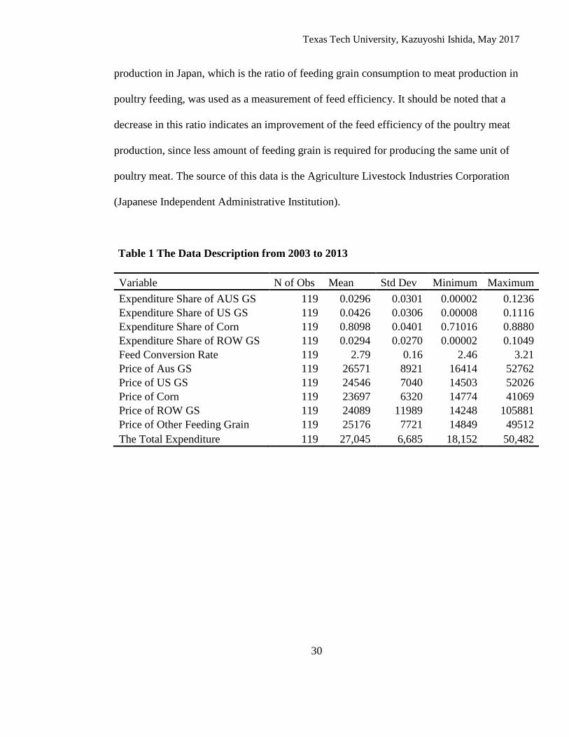
Table 1 The Data Description from 2003 to 2013
Variable N of Obs Mean Std Dev Minimum Maximum Expenditure Share of AUS GS 119 0.0296 0.0301 0.00002 0.1236 Expenditure Share of US GS 119 0.0426 0.0306 0.00008 0.1116 Expenditure Share of Corn 119 0.8098 0.0401 0.71016 0.8880 Expenditure Share of ROW GS 119 0.0294 0.0270 0.00002 0.1049 Feed Conversion Rate 119 2.79 0.16 2.46 3.21 Price of Aus GS 119 26571 8921 16414 52762 Price of US GS 119 24546 7040 14503 52026 Price of Corn 119 23697 6320 14774 41069 Price of ROW GS 119 24089 11989 14248 105881 Price of Other Feeding Grain 119 25176 7721 14849 49512 The Total Expenditure 119 27,045 6,685 18,152 50,482
Texas Tech University, Kazuyoshi Ishida, May 2017
31
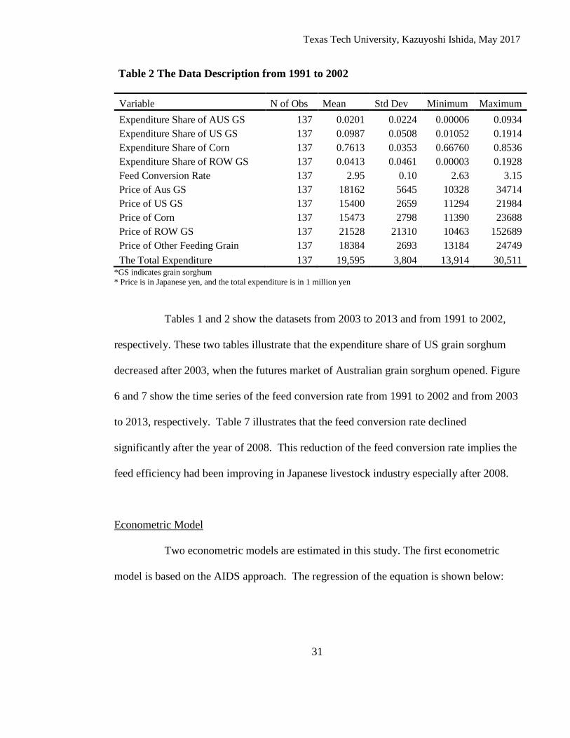
Table 2 The Data Description from 1991 to 2002
Variable N of Obs Mean Std Dev Minimum Maximum Expenditure Share of AUS GS 137 0.0201 0.0224 0.00006 0.0934 Expenditure Share of US GS 137 0.0987 0.0508 0.01052 0.1914 Expenditure Share of Corn 137 0.7613 0.0353 0.66760 0.8536 Expenditure Share of ROW GS 137 0.0413 0.0461 0.00003 0.1928 Feed Conversion Rate 137 2.95 0.10 2.63 3.15 Price of Aus GS 137 18162 5645 10328 34714 Price of US GS 137 15400 2659 11294 21984 Price of Corn 137 15473 2798 11390 23688 Price of ROW GS 137 21528 21310 10463 152689 Price of Other Feeding Grain 137 18384 2693 13184 24749 The Total Expenditure 137 19,595 3,804 13,914 30,511
*GS indicates grain sorghum * Price is in Japanese yen, and the total expenditure is in 1 million yen
Tables 1 and 2 show the datasets from 2003 to 2013 and from 1991 to 2002,
respectively. These two tables illustrate that the expenditure share of US grain sorghum
decreased after 2003, when the futures market of Australian grain sorghum opened. Figure
6 and 7 show the time series of the feed conversion rate from 1991 to 2002 and from 2003
to 2013, respectively. Table 7 illustrates that the feed conversion rate declined
significantly after the year of 2008. This reduction of the feed conversion rate implies the
feed efficiency had been improving in Japanese livestock industry especially after 2008.
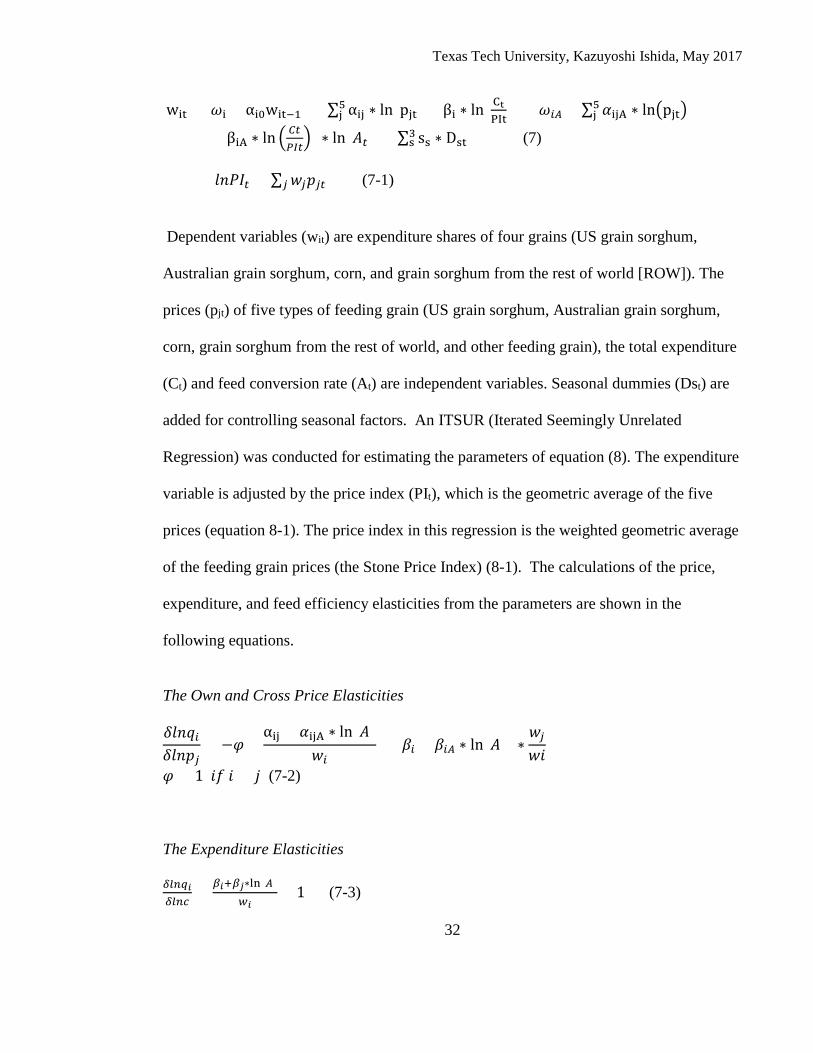
Econometric Model
Two econometric models are estimated in this study. The first econometric
model is based on the AIDS approach. The regression of the equation is shown below:
Texas Tech University, Kazuyoshi Ishida, May 2017
32
wit = 𝜔𝜔i + αi0wit−1 + ∑ αij ∗ ln(pjt) + βi ∗ ln ( CtPIt
) + (𝜔𝜔𝑖𝑖𝐴𝐴 + ∑ 𝛼𝛼ijA ∗ lnpjt5j
5j
+βiA ∗ ln 𝐶𝐶𝐶𝐶𝛿𝛿𝑃𝑃𝐶𝐶) ∗ ln (𝐴𝐴𝐶𝐶) +∑ ss ∗ Dst
3s (7)
𝑙𝑙𝑙𝑙𝑃𝑃𝑃𝑃𝐶𝐶 = ∑ 𝑤𝑤𝑗𝑗𝑝𝑝𝑗𝑗𝐶𝐶𝑗𝑗 (7-1) Dependent variables (wit) are expenditure shares of four grains (US grain sorghum,
Australian grain sorghum, corn, and grain sorghum from the rest of world [ROW]). The
prices (pjt) of five types of feeding grain (US grain sorghum, Australian grain sorghum,
corn, grain sorghum from the rest of world, and other feeding grain), the total expenditure
(Ct) and feed conversion rate (At) are independent variables. Seasonal dummies (Dst) are
added for controlling seasonal factors. An ITSUR (Iterated Seemingly Unrelated
Regression) was conducted for estimating the parameters of equation (8). The expenditure
variable is adjusted by the price index (PIt), which is the geometric average of the five
prices (equation 8-1). The price index in this regression is the weighted geometric average
of the feeding grain prices (the Stone Price Index) (8-1). The calculations of the price,
expenditure, and feed efficiency elasticities from the parameters are shown in the
following equations.
The Own and Cross Price Elasticities 𝛿𝛿𝑙𝑙𝑙𝑙𝑞𝑞𝑖𝑖𝛿𝛿𝑙𝑙𝑙𝑙𝑝𝑝𝑗𝑗
= −𝜑𝜑 +αij + 𝛼𝛼ijA ∗ ln(𝐴𝐴)
𝑤𝑤𝑖𝑖+ (𝛽𝛽𝑖𝑖 + 𝛽𝛽𝑖𝑖𝐴𝐴 ∗ ln(𝐴𝐴)) ∗
𝑤𝑤𝑗𝑗𝑤𝑤𝑄𝑄
𝜑𝜑 = 1 𝑄𝑄𝑓𝑓 𝑄𝑄 = 𝑗𝑗 (7-2) The Expenditure Elasticities 𝛿𝛿𝑙𝑙𝑙𝑙𝑞𝑞𝑖𝑖𝛿𝛿𝑙𝑙𝑙𝑙𝛿𝛿
= 𝛽𝛽𝑖𝑖+𝛽𝛽𝑗𝑗∗ln (𝐴𝐴)𝑤𝑤𝑖𝑖
+ 1 (7-3)
Texas Tech University, Kazuyoshi Ishida, May 2017
33
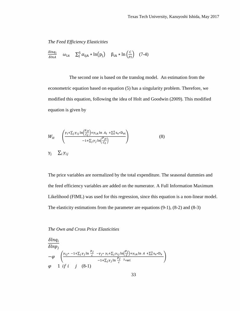
The Feed Efficiency Elasticities 𝛿𝛿𝑙𝑙𝑙𝑙𝑞𝑞𝑖𝑖𝛿𝛿𝑙𝑙𝑙𝑙𝐴𝐴
= 𝜔𝜔𝑖𝑖𝐴𝐴 + ∑ 𝛼𝛼ijA ∗ lnpj5j + βiA ∗ ln 𝐶𝐶
𝛿𝛿𝑃𝑃 (7-4)
The second one is based on the translog model. An estimation from the
econometric equation based on equation (5) has a singularity problem. Therefore, we
modified this equation, following the idea of Holt and Goodwin (2009). This modified
equation is given by
𝑊𝑊𝑖𝑖𝐶𝐶 = 𝛾𝛾𝑖𝑖+∑ 𝛾𝛾𝑖𝑖𝑗𝑗𝑗𝑗 ln
𝑝𝑝𝑗𝑗𝑗𝑗𝑗𝑗𝑗𝑗+𝛾𝛾𝑖𝑖𝑘𝑘 ln(𝐴𝐴𝑗𝑗)+∑ ss∗Dst3
s
−1+∑ 𝛾𝛾𝑗𝑗𝑗𝑗 ln𝑃𝑃𝑗𝑗𝑗𝑗𝑗𝑗𝑗𝑗
(8)
γj = ∑ 𝛾𝛾𝑖𝑖𝑗𝑗𝑖𝑖
The price variables are normalized by the total expenditure. The seasonal dummies and
the feed efficiency variables are added on the numerator. A Full Information Maximum
Likelihood (FIML) was used for this regression, since this equation is a non-linear model.
The elasticity estimations from the parameter are equations (9-1), (8-2) and (8-3)
The Own and Cross Price Elasticities
𝛿𝛿𝑙𝑙𝑙𝑙𝑞𝑞𝑖𝑖𝛿𝛿𝑙𝑙𝑙𝑙𝑝𝑝𝑗𝑗
=
−𝜑𝜑 + 𝛾𝛾𝑖𝑖𝑗𝑗∗(−1+∑ 𝛾𝛾𝑗𝑗 ln(
𝑝𝑝𝑗𝑗𝑖𝑖 )𝑗𝑗 )−𝛾𝛾𝑗𝑗∗(𝛾𝛾𝑖𝑖+∑ 𝛾𝛾𝑖𝑖𝑗𝑗𝑗𝑗 ln
𝑝𝑝𝑗𝑗𝑗𝑗 +𝛾𝛾𝑖𝑖𝑘𝑘 ln(𝐴𝐴)+∑ ss∗Ds3
s )
(−1+∑ 𝛾𝛾𝑗𝑗 ln(𝑝𝑝𝑗𝑗𝑖𝑖 )𝑗𝑗 )2∗𝑤𝑤𝑖𝑖
𝜑𝜑 = 1 𝑄𝑄𝑓𝑓 𝑄𝑄 = 𝑗𝑗 (8-1)
Texas Tech University, Kazuyoshi Ishida, May 2017
34
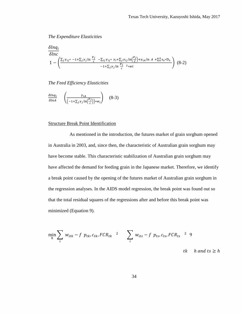
The Expenditure Elasticities 𝛿𝛿𝑙𝑙𝑙𝑙𝑞𝑞𝑖𝑖𝛿𝛿𝑙𝑙𝑙𝑙𝑃𝑃
=
1 − ∑ 𝛾𝛾𝑖𝑖𝑗𝑗∗(−1+∑ 𝛾𝛾𝑗𝑗 ln(
𝑝𝑝𝑗𝑗𝑖𝑖 )𝑗𝑗 )𝑗𝑗 −∑ 𝛾𝛾𝑖𝑖𝑗𝑗𝑖𝑖𝑗𝑗 ∗(𝛾𝛾𝑖𝑖+∑ 𝛾𝛾𝑖𝑖𝑗𝑗𝑗𝑗 ln
𝑝𝑝𝑗𝑗𝑗𝑗 +𝛾𝛾𝑖𝑖𝑘𝑘 ln(𝐴𝐴)+∑ ss∗Ds)3
s
(−1+∑ 𝛾𝛾𝑗𝑗 ln(𝑝𝑝𝑗𝑗𝑖𝑖 )𝑗𝑗 )2∗𝑤𝑤𝑖𝑖
(8-2)
The Feed Efficiency Elasticities 𝛿𝛿𝑙𝑙𝑙𝑙𝑞𝑞𝑖𝑖𝛿𝛿𝑙𝑙𝑙𝑙𝐴𝐴
= 𝛾𝛾𝑖𝑖𝑘𝑘−1+∑ 𝛾𝛾𝑗𝑗 ln
𝑝𝑝𝑗𝑗𝑖𝑖 𝑗𝑗 ∗𝑤𝑤𝑖𝑖
(8-3)
Structure Break Point Identification
As mentioned in the introduction, the futures market of grain sorghum opened
in Australia in 2003, and, since then, the characteristic of Australian grain sorghum may
have become stable. This characteristic stabilization of Australian grain sorghum may
have affected the demand for feeding grain in the Japanese market. Therefore, we identify
a break point caused by the opening of the futures market of Australian grain sorghum in
the regression analyses. In the AIDS model regression, the break point was found out so
that the total residual squares of the regressions after and before this break point was
minimized (Equation 9).
minℎ(𝑤𝑤𝑖𝑖𝐶𝐶𝑖𝑖 − 𝑓𝑓(𝑝𝑝𝐶𝐶𝑖𝑖, 𝑃𝑃𝐶𝐶𝑖𝑖,𝐹𝐹𝐶𝐶𝑅𝑅𝐶𝐶𝑖𝑖))2 𝑖𝑖
+ (𝑤𝑤𝑖𝑖𝐶𝐶𝑠𝑠 − 𝑓𝑓(𝑝𝑝𝐶𝐶𝑠𝑠, 𝑃𝑃𝐶𝐶𝑠𝑠,𝐹𝐹𝐶𝐶𝑅𝑅𝐶𝐶𝑠𝑠))2 (9) 𝑖𝑖
𝑄𝑄𝑘𝑘 < ℎ 𝑄𝑄𝑙𝑙𝑎𝑎 𝑄𝑄𝐸𝐸 ≥ ℎ
Texas Tech University, Kazuyoshi Ishida, May 2017
35
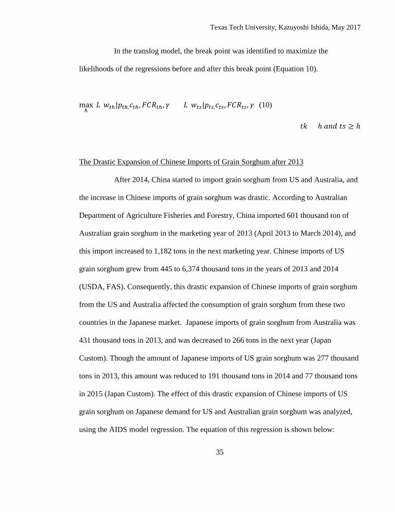
In the translog model, the break point was identified to maximize the
likelihoods of the regressions before and after this break point (Equation 10).
maxℎ
𝐿𝐿(𝑤𝑤𝐶𝐶ℎ|𝑝𝑝𝐶𝐶ℎ,𝑃𝑃𝐶𝐶ℎ,𝐹𝐹𝐶𝐶𝑅𝑅𝐶𝐶ℎ , 𝛾𝛾) + 𝐿𝐿(𝑤𝑤𝐶𝐶𝑠𝑠|𝑝𝑝𝐶𝐶𝑠𝑠,𝑃𝑃𝐶𝐶𝑠𝑠,𝐹𝐹𝐶𝐶𝑅𝑅𝐶𝐶𝑠𝑠, 𝛾𝛾) (10)
𝑄𝑄𝑘𝑘 < ℎ 𝑄𝑄𝑙𝑙𝑎𝑎 𝑄𝑄𝐸𝐸 ≥ ℎ
The Drastic Expansion of Chinese Imports of Grain Sorghum after 2013
After 2014, China started to import grain sorghum from US and Australia, and
the increase in Chinese imports of grain sorghum was drastic. According to Australian
Department of Agriculture Fisheries and Forestry, China imported 601 thousand ton of
Australian grain sorghum in the marketing year of 2013 (April 2013 to March 2014), and
this import increased to 1,182 tons in the next marketing year. Chinese imports of US
grain sorghum grew from 445 to 6,374 thousand tons in the years of 2013 and 2014
(USDA, FAS). Consequently, this drastic expansion of Chinese imports of grain sorghum
from the US and Australia affected the consumption of grain sorghum from these two
countries in the Japanese market. Japanese imports of grain sorghum from Australia was
431 thousand tons in 2013, and was decreased to 266 tons in the next year (Japan
Custom). Though the amount of Japanese imports of US grain sorghum was 277 thousand
tons in 2013, this amount was reduced to 191 thousand tons in 2014 and 77 thousand tons
in 2015 (Japan Custom). The effect of this drastic expansion of Chinese imports of US
grain sorghum on Japanese demand for US and Australian grain sorghum was analyzed,
using the AIDS model regression. The equation of this regression is shown below:
Texas Tech University, Kazuyoshi Ishida, May 2017
36
wit = 𝜔𝜔i + αi0wit−1 + ∑ αij + kij ∗ CImpt ∗ lnpjt + (βi + hi ∗ CImpt) ∗ ln (Ctpt
) +5j
(𝜔𝜔𝑖𝑖𝐴𝐴 + ∑ 𝛼𝛼ijA ∗ lnpjt5j + βiA ∗ ln 𝐶𝐶𝐶𝐶
𝛿𝛿𝑃𝑃𝐶𝐶) ∗ ln (𝐴𝐴𝐶𝐶) + ∑ ss ∗ Dst
3s (9)
𝑙𝑙𝑙𝑙𝑃𝑃𝑃𝑃𝐶𝐶 = ∑ 𝑤𝑤𝑗𝑗𝑝𝑝𝑗𝑗𝐶𝐶𝑗𝑗 (9-1) 𝐶𝐶𝑃𝑃𝐶𝐶𝑝𝑝𝐶𝐶 = 1 𝑄𝑄𝑓𝑓 𝑙𝑙𝑦𝑦𝑄𝑄𝑟𝑟 ≥ 2014, 𝑜𝑜𝑄𝑄ℎ𝑦𝑦𝑟𝑟𝑤𝑤𝑄𝑄𝐸𝐸𝑦𝑦 0 (9-2)
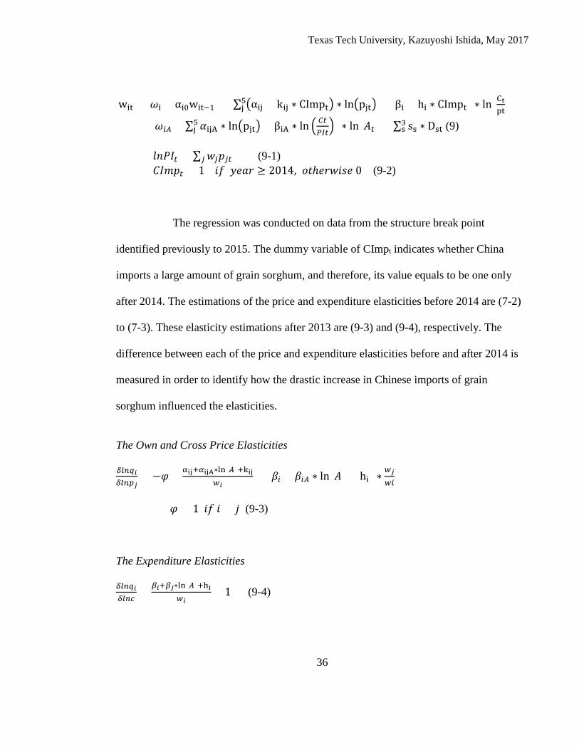
The regression was conducted on data from the structure break point
identified previously to 2015. The dummy variable of CImpt indicates whether China
imports a large amount of grain sorghum, and therefore, its value equals to be one only
after 2014. The estimations of the price and expenditure elasticities before 2014 are (7-2)
to (7-3). These elasticity estimations after 2013 are (9-3) and (9-4), respectively. The
difference between each of the price and expenditure elasticities before and after 2014 is
measured in order to identify how the drastic increase in Chinese imports of grain
sorghum influenced the elasticities.
The Own and Cross Price Elasticities 𝛿𝛿𝑙𝑙𝑙𝑙𝑞𝑞𝑖𝑖𝛿𝛿𝑙𝑙𝑙𝑙𝑝𝑝𝑗𝑗
= −𝜑𝜑 + αij+𝛼𝛼ijA∗ln(𝐴𝐴)+kij𝑤𝑤𝑖𝑖
+ (𝛽𝛽𝑖𝑖 + 𝛽𝛽𝑖𝑖𝐴𝐴 ∗ ln(𝐴𝐴) + hi) ∗𝑤𝑤𝑗𝑗
𝑤𝑤𝑖𝑖
𝜑𝜑 = 1 𝑄𝑄𝑓𝑓 𝑄𝑄 = 𝑗𝑗 (9-3) The Expenditure Elasticities 𝛿𝛿𝑙𝑙𝑙𝑙𝑞𝑞𝑖𝑖𝛿𝛿𝑙𝑙𝑙𝑙𝛿𝛿
= 𝛽𝛽𝑖𝑖+𝛽𝛽𝑗𝑗∗ln(𝐴𝐴)+hi𝑤𝑤𝑖𝑖
+ 1 (9-4)
Texas Tech University, Kazuyoshi Ishida, May 2017
37
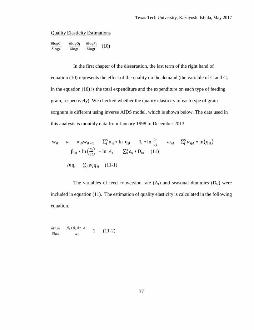
Quality Elasticity Estimations
δlogCiδlogC
= δlogQiδlogC
+ δlogPiδlogC
(10)
In the first chapter of the dissertation, the last term of the right hand of
equation (10) represents the effect of the quality on the demand (the variable of C and Ci
in the equation (10) is the total expenditure and the expenditure on each type of feeding
grain, respectively). We checked whether the quality elasticity of each type of grain
sorghum is different using inverse AIDS model, which is shown below. The data used in
this analysis is monthly data from January 1998 to December 2013.
wit = 𝜔𝜔i + αi0wit−1 + ∑ αij ∗ ln(qjt) + βi ∗ ln (ct
qt) + (𝜔𝜔𝑖𝑖𝐴𝐴 + ∑ 𝛼𝛼ijA ∗ lnqjt5
j5j
+βiA ∗ ln 𝛿𝛿𝑗𝑗𝑞𝑞𝐶𝐶) ∗ ln (𝐴𝐴𝐶𝐶) +∑ ss ∗ Dst
3s (11)
𝑙𝑙𝑙𝑙𝑞𝑞𝐶𝐶 = ∑ 𝑤𝑤𝑗𝑗𝑞𝑞𝑗𝑗𝐶𝐶𝑗𝑗 (11-1)
The variables of feed conversion rate (At) and seasonal dummies (Dst) were
included in equation (11). The estimation of quality elasticity is calculated in the following
equation.
𝛿𝛿𝑙𝑙𝑙𝑙𝑝𝑝𝑖𝑖𝛿𝛿𝑙𝑙𝑙𝑙𝛿𝛿
= 𝛽𝛽𝑖𝑖+𝛽𝛽𝑗𝑗∗ln (𝐴𝐴)𝑤𝑤𝑖𝑖
+ 1 (11-2)
Texas Tech University, Kazuyoshi Ishida, May 2017
38
Random Estimations of the Elasticities
It is difficult to assume that, in the Japanese feeding grain market, the response
of the demand of each feeding grain to changes in feeding grain prices and the total
expenditure are always the same. Therefore, the price, expenditure and feed efficiency
elasticities of each type of feeding grain may be random over certain distributions.
Consequently, the random estimations of the elasticities were conducted using the
Bayesian seemingly unrelated regression (SUR) based on the AIDS model (equation (7-
1)). A Bayesian regression was used for the demand analysis of alcoholic beverage by
Lariviere, Larue, and Chalfant (2000), and the analysis of electronic demand by Xiao,
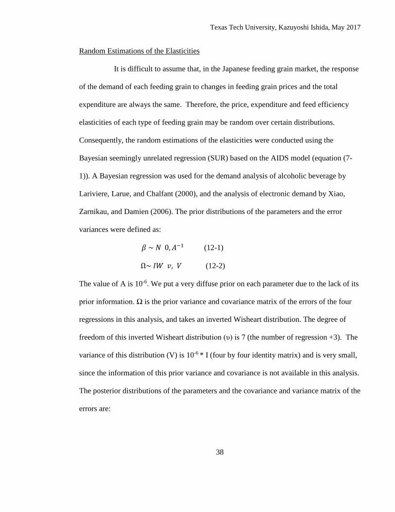
Zarnikau, and Damien (2006). The prior distributions of the parameters and the error
variances were defined as:
𝛽𝛽 ~ 𝑁𝑁(0,𝐴𝐴−1) (12-1)
Ω~ 𝑃𝑃𝑊𝑊(𝑣𝑣, 𝑉𝑉) (12-2)
The value of A is 10-6. We put a very diffuse prior on each parameter due to the lack of its
prior information. Ω is the prior variance and covariance matrix of the errors of the four
regressions in this analysis, and takes an inverted Wisheart distribution. The degree of
freedom of this inverted Wisheart distribution (υ) is 7 (the number of regression +3). The
variance of this distribution (V) is 10-6 * I (four by four identity matrix) and is very small,
since the information of this prior variance and covariance is not available in this analysis.
The posterior distributions of the parameters and the covariance and variance matrix of the
errors are:
Texas Tech University, Kazuyoshi Ishida, May 2017
39
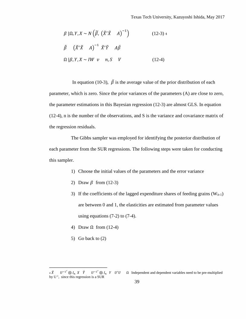
𝛽𝛽 |Ω,𝑌𝑌,𝑋𝑋 ~ 𝑁𝑁 𝛽𝛽, 𝑋𝑋′𝑋𝑋 + 𝐴𝐴−1 (12-3) 4
𝛽𝛽 = 𝑋𝑋′𝑋𝑋 + 𝐴𝐴−1
(𝑋𝑋′𝑌𝑌 + 𝐴𝐴𝛽)
Ω |𝛽𝛽,𝑌𝑌,𝑋𝑋 ~ 𝑃𝑃𝑊𝑊(𝑣𝑣 + 𝑙𝑙, 𝑆𝑆 + 𝑉𝑉) (12-4)
In equation (10-3), 𝛽 is the average value of the prior distribution of each
parameter, which is zero. Since the prior variances of the parameters (A) are close to zero,
the parameter estimations in this Bayesian regression (12-3) are almost GLS. In equation
(12-4), n is the number of the observations, and S is the variance and covariance matrix of
the regression residuals.
The Gibbs sampler was employed for identifying the posterior distribution of
each parameter from the SUR regressions. The following steps were taken for conducting
this sampler.
1) Choose the initial values of the parameters and the error variance
2) Draw 𝛽𝛽 from (12-3)
3) If the coefficients of the lagged expenditure shares of feeding grains (Wit-1)
are between 0 and 1, the elasticities are estimated from parameter values
using equations (7-2) to (7-4).
4) Draw Ω from (12-4)
5) Go back to (2)
4 𝑋𝑋 = (𝑈𝑈−1′ ⊗ 𝑃𝑃𝑙𝑙)𝑋𝑋 𝑌𝑌 = (𝑈𝑈−1′ ⊗ 𝑃𝑃𝑙𝑙) 𝑌𝑌 𝑈𝑈′𝑈𝑈 = Ω Independent and dependent variables need to be pre-multiplied by U-1, since this regression is a SUR
Texas Tech University, Kazuyoshi Ishida, May 2017
40
The steps (1) to (5) were conducted 100,000 times. As shown in step (4), restrictions were
put on the parameter values of the lagged dependent variables. The first 10,000 elasticity
estimations were discarded for deleting the effect of the initial values of the parameters
and error variance on these estimations. The posterior distributions of the elasticities were
identified from the estimations of the remaining iterations.
Results
Results of the AIDS Model Regression
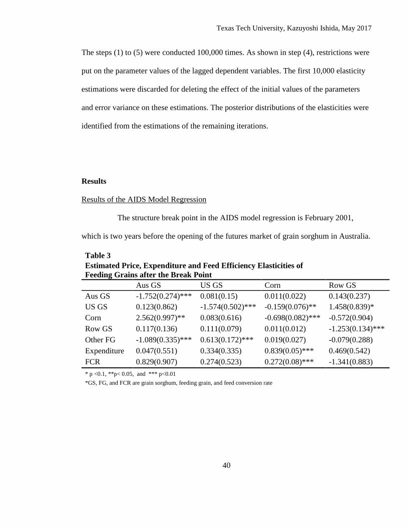
The structure break point in the AIDS model regression is February 2001,
which is two years before the opening of the futures market of grain sorghum in Australia.
Table 3 Estimated Price, Expenditure and Feed Efficiency Elasticities of Feeding Grains after the Break Point Aus GS US GS Corn Row GS Aus GS -1.752(0.274)*** 0.081(0.15) 0.011(0.022) 0.143(0.237) US GS 0.123(0.862) -1.574(0.502)*** -0.159(0.076)** 1.458(0.839)* Corn 2.562(0.997)** 0.083(0.616) -0.698(0.082)*** -0.572(0.904) Row GS 0.117(0.136) 0.111(0.079) 0.011(0.012) -1.253(0.134)*** Other FG -1.089(0.335)*** 0.613(0.172)*** 0.019(0.027) -0.079(0.288) Expenditure 0.047(0.551) 0.334(0.335) 0.839(0.05)*** 0.469(0.542) FCR 0.829(0.907) 0.274(0.523) 0.272(0.08)*** -1.341(0.883) * p <0.1, **p< 0.05, and *** p<0.01 *GS, FG, and FCR are grain sorghum, feeding grain, and feed conversion rate
Texas Tech University, Kazuyoshi Ishida, May 2017
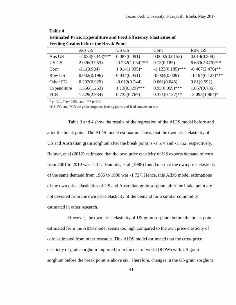
41
Table 4 Estimated Price, Expenditure and Feed Efficiency Elasticities of Feeding Grains before the Break Point Aus GS US GS Corn Row GS Aus GS -2.023(0.343)*** 0.087(0.091) 0.0002(0.0153) 0.014(0.209) US GS 2.026(3.953) -3.232(1.034)*** 0.13(0.185) 6.683(2.479)*** Corn -2.1(3.984) 1.914(1.035)* -1.123(0.185)*** -6.467(2.476)** Row GS 0.032(0.196) 0.034(0.051) -0.004(0.009) -1.194(0.127)*** Other FG 0.292(0.929) -0.012(0.244) 0.061(0.045) 0.81(0.592) Expenditure 1.566(1.263) 1.13(0.329)*** 0.95(0.059)*** 1.067(0.786) FCR 1.529(2.934) 0.732(0.767) 0.321(0.137)** -3.098(1.864)* * p <0.1, **p< 0.05, and *** p<0.01 *GS, FG, and FCR are grain sorghum, feeding grain, and feed conversion rate
Table 3 and 4 show the results of the regression of the AIDS model before and
after the break point. The AIDS model estimation shows that the own price elasticity of
US and Australian grain sorghum after the break point is -1.574 and -1.752, respectively.
Reimer, et al (2012) estimated that the own price elasticity of US exports demand of corn
from 2001 to 2010 was -1.11. Haniotis, et al (1988) found out that the own price elasticity
of the same demand from 1965 to 1986 was -1.727. Hence, this AIDS model estimations
of the own price elasticities of US and Australian grain sorghum after the brake point are
not deviated from the own price elasticity of the demand for a similar commodity
estimated in other research.
However, the own price elasticity of US grain sorghum before the break point
estimated from the AIDS model seems too high compared to the own price elasticity of
corn estimated from other research. This AIDS model estimated that the cross price
elasticity of grain sorghum imported from the rest of world (ROW) with US grain
sorghum before the break point is above six. Therefore, changes in the US grain sorghum
Texas Tech University, Kazuyoshi Ishida, May 2017
42
price might have affected the demand for US and ROW grain sorghum heavily.
Approximately 90% of grain sorghum in the Japanese market imported from US and the
rest of world before the break point (Japan Customs, 2016). This result indicates that the
quality differential of grain sorghum from each country might have been smaller
compared to that of corn before the break point, and the price differential of grain
sorghum from each country might have influenced its demand during that period.
Table 3 shows that the estimated cross price elasticity of Australian grain
sorghum with respect to US grain sorghum after the break point is not statistically
significant at 95% confidence level. This result indicates that changes in the price of US
grain sorghum might not have affected the demand for Australian grain sorghum after the
break point. Therefore, the recent increases in US grain sorghum price may not expand the
market share of Australian grain sorghum, and may not be a factor of the declining market
share of US grain sorghum in the Japanese market.
The estimated cross price elasticities of Australian and US grain sorghum with
respect to corn before the break point are not statistically significant. The estimated cross
price elasticity of Australian grain sorghum with respect to corn after the break point is
positive and statistically significant, and, on the other hand, the cross price elasticity of US
grain sorghum with corn over the same years is not significant. Therefore, the cross price
elasticity of Australian grain sorghum with respect to corn may have become larger than
that of US grain sorghum after the break point.
One reason that US grain sorghum lost its market share in the Japanese market
may be that the substitutability of Australian grain sorghum with corn may have become
Texas Tech University, Kazuyoshi Ishida, May 2017
43
stronger. This estimation indicates that an increase in the corn price may lead to a positive
change in the demand for Australian grain sorghum in the Japanese market. The trend of
the corn price has been upward due to the corn ethanol demand in the world market after
the year of 2008 (See figure 4). Hence, in order to prevent the price of their product from
rising too high, Japanese formula feed producers might have decreased their consumption
of corn (See figure 3), and purchased other kinds of feeding grain instead. Australian grain
sorghum may be a good alternative for corn, because its quality has become more stable
and reliable after the opening of its futures market in Australia. Figure 5 shows that the
consumption of US grain sorghum was on the downward trend in Japan after the break
point. On the other hand, the same figure illustrates that the demand for Australian grain
sorghum did not decrease. During these years, the prices of Australian and US grain
sorghum went up (See figure 2). From our estimation of the own price elasticity of
Australian grain sorghum, an increase in the price of Australian grain sorghum has a
negative effect on its quantity demanded. However, according to the estimated cross price
elasticity of Australian grain sorghum with respect to corn, the demand for Australian grain
sorghum may have been expanded by the upward trend of the corn price in the Japanese
market at that same time. This can explain why the quantity demanded for Australian grain
sorghum did not decrease even though its price rose up in the Japanese market after 2008.
The result of the regression after the break point suggests that the effects of a
change in the feed conversion rate on the demands for US and Australian grain sorghum are
larger than the effect on the demand for corn. However, these estimated effects are not
statistically significant due to their large standard errors. Hence, the effects of the efficiency
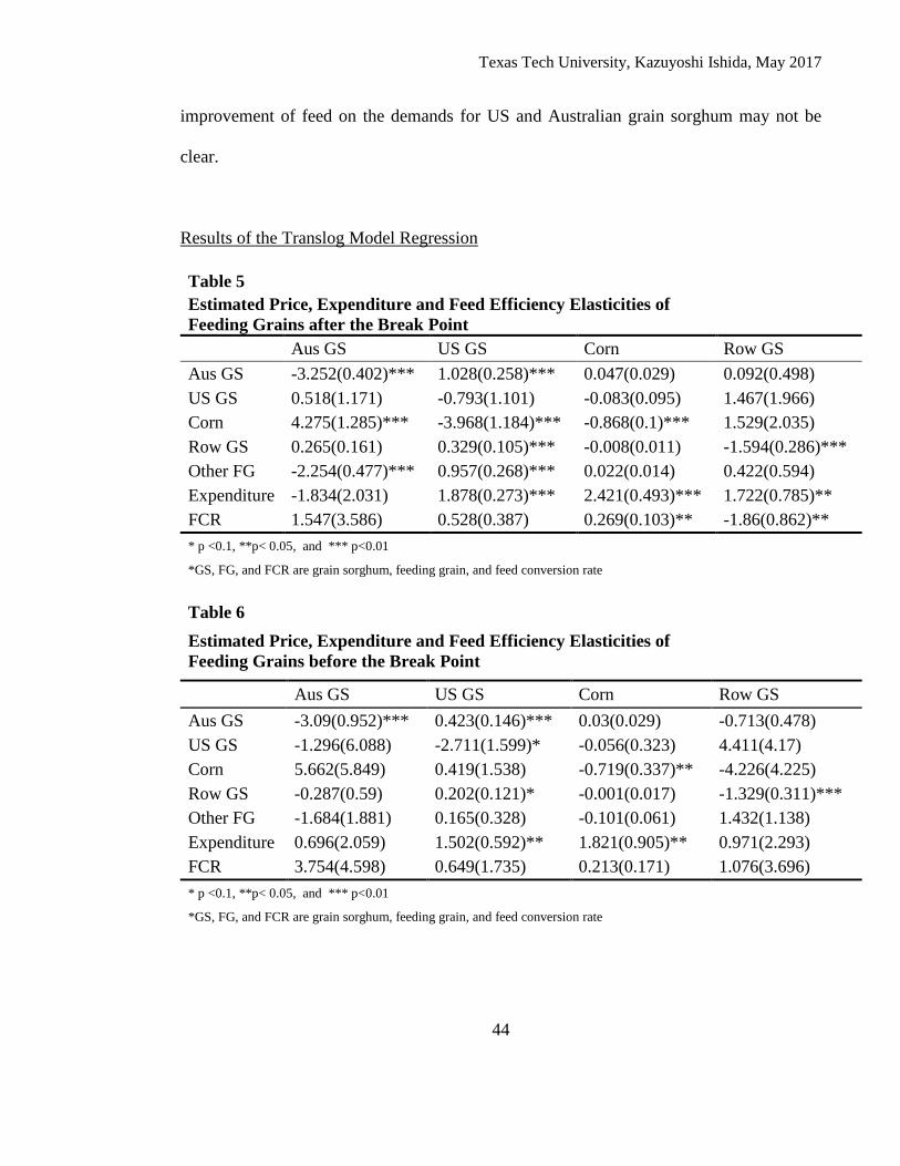
Texas Tech University, Kazuyoshi Ishida, May 2017
44
improvement of feed on the demands for US and Australian grain sorghum may not be
clear.
Results of the Translog Model Regression
Table 5 Estimated Price, Expenditure and Feed Efficiency Elasticities of Feeding Grains after the Break Point Aus GS US GS Corn Row GS Aus GS -3.252(0.402)*** 1.028(0.258)*** 0.047(0.029) 0.092(0.498) US GS 0.518(1.171) -0.793(1.101) -0.083(0.095) 1.467(1.966) Corn 4.275(1.285)*** -3.968(1.184)*** -0.868(0.1)*** 1.529(2.035) Row GS 0.265(0.161) 0.329(0.105)*** -0.008(0.011) -1.594(0.286)*** Other FG -2.254(0.477)*** 0.957(0.268)*** 0.022(0.014) 0.422(0.594) Expenditure -1.834(2.031) 1.878(0.273)*** 2.421(0.493)*** 1.722(0.785)** FCR 1.547(3.586) 0.528(0.387) 0.269(0.103)** -1.86(0.862)** * p <0.1, **p< 0.05, and *** p<0.01
*GS, FG, and FCR are grain sorghum, feeding grain, and feed conversion rate
Table 6 Estimated Price, Expenditure and Feed Efficiency Elasticities of Feeding Grains before the Break Point
Aus GS US GS Corn Row GS Aus GS -3.09(0.952)*** 0.423(0.146)*** 0.03(0.029) -0.713(0.478) US GS -1.296(6.088) -2.711(1.599)* -0.056(0.323) 4.411(4.17) Corn 5.662(5.849) 0.419(1.538) -0.719(0.337)** -4.226(4.225) Row GS -0.287(0.59) 0.202(0.121)* -0.001(0.017) -1.329(0.311)*** Other FG -1.684(1.881) 0.165(0.328) -0.101(0.061) 1.432(1.138) Expenditure 0.696(2.059) 1.502(0.592)** 1.821(0.905)** 0.971(2.293) FCR 3.754(4.598) 0.649(1.735) 0.213(0.171) 1.076(3.696) * p <0.1, **p< 0.05, and *** p<0.01
*GS, FG, and FCR are grain sorghum, feeding grain, and feed conversion rate
Texas Tech University, Kazuyoshi Ishida, May 2017
45
The break point for the translog model was May 2000. Tables 5 and 6
illustrate the price, expenditure and feed efficiency elasticities estimated from the translog
morel regression. Compared to the AIDS model estimation, the own price elasticities of
Australian grain sorghum estimated from the translog model after the break point (-3.252)
are smaller. Therefore, the price elasticity measured by this model is largely deviated
from the price elasticity estimations of a similar demand (the export demand of US corn)
conducted by other researchers.
The R-square of the AIDS model regression in both the two periods goes from
40% to 80%, and, on the other hands, the R-Squares of the translog model regression are
20% to 60%. The AIC values of the AIDS and the translog model regressions are -
6691.86 and -6769.8, respectively. Therefore, the goodness of the AIDS model on the data
is higher.
In the results of the translog model regression, the cross price elasticity of
Australian grain sorghum with corn and vice versa in the period after the break point is
statistically positively significant in the 95% confidence level. The same cross price
elasticities in the period before the break point are not significant. On the other hand, the
cross price elasticities of US sorghum with corn before and after the break point and vice
versa are not significant. The estimations of these cross price elasticities from the translog
model are the same as those from the regression analysis of the AIDS model. This result
of the translog model confirms that Australian grain sorghum has become a substitute
good for corn after the year of 1998.
Texas Tech University, Kazuyoshi Ishida, May 2017
46
The cross price elasticities of US grain sorghum with Australian grain sorghum
are statistically positively significant in the translog model regressions in the two periods,
but its vice versa is not. This model estimates that the own price elasticity of US grain
sorghum is not significant, and the own price elasticity of the Australian grain sorghum is
significant and negative. Figure 2 illustrates that the prices of US and Australian grain
sorghum were on the upward trend after the break point. The results of the translog model
regression indicate that the upward trends of these prices had a positive impact on the US
grain sorghum demand in the Japanese market, and had a negative impact on the demand
for Australian grain sorghum. The cross price elasticity of US grain sorghum with respect
to the price of Australian grain sorghum estimated in the translog model indicates that the
upward trend of the price of Australian grain sorghum might influence the demand for US
grain sorghum positively, On the other hand, the increase in the price of US grain
sorghum might not affect the demand for Australian grain sorghum.
Separability Condition
We examined the validity of the separation of the grain sorghum goods’ group.
The grain sorghum goods’ group are composed of US, Australia, and ROW sorghum. This
separability condition examination is based on the following equation.
𝑆𝑆𝑘𝑘𝑗𝑗𝛿𝛿𝑞𝑞𝑘𝑘𝛿𝛿𝑥𝑥
= 𝑆𝑆𝑖𝑖𝑗𝑗𝛿𝛿𝑞𝑞𝑖𝑖𝛿𝛿𝑥𝑥
∀ 𝑄𝑄,𝑘𝑘 ∈ 𝑟𝑟 (13)
In this equation, the variable r and j are the sorghum goods’ group and other kinds of
feeding grain respectively. Skj is defined as the Hicksian substitution between a certain
type of sorghum (k) and other type of feeding grain (j). 𝛿𝛿𝑞𝑞𝑘𝑘𝛿𝛿𝑙𝑙
is the income elasticity of this
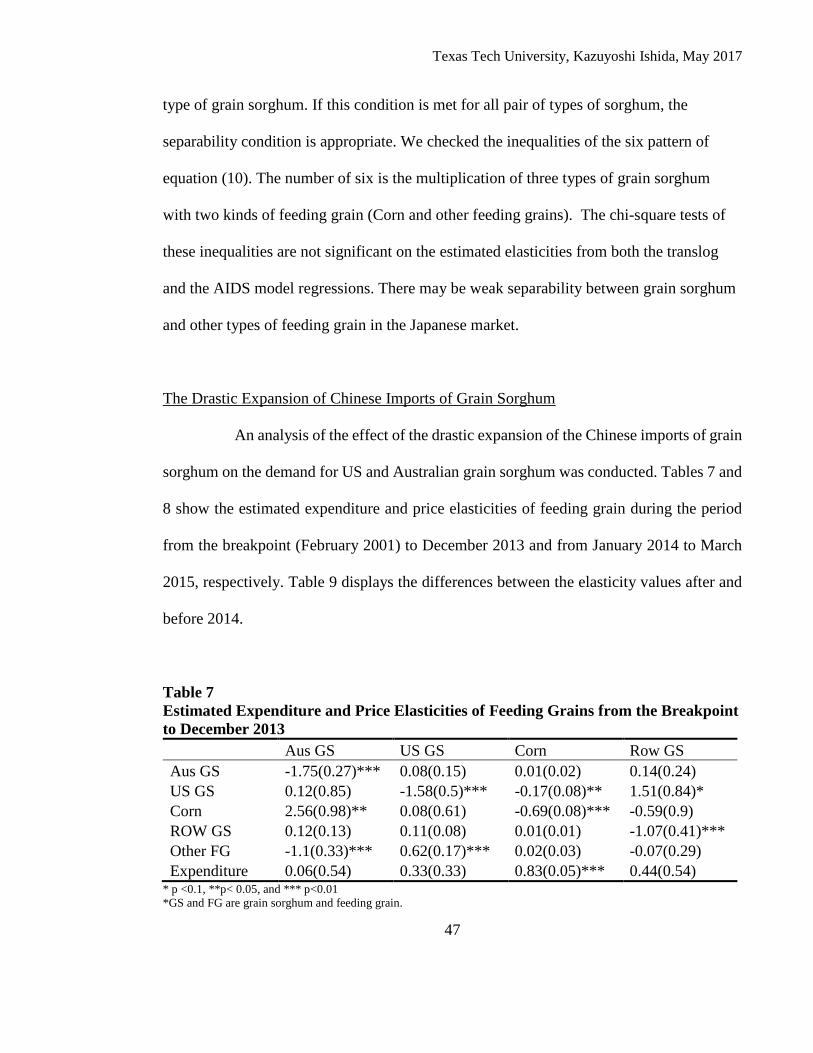
Texas Tech University, Kazuyoshi Ishida, May 2017
47
type of grain sorghum. If this condition is met for all pair of types of sorghum, the
separability condition is appropriate. We checked the inequalities of the six pattern of
equation (10). The number of six is the multiplication of three types of grain sorghum
with two kinds of feeding grain (Corn and other feeding grains). The chi-square tests of
these inequalities are not significant on the estimated elasticities from both the translog
and the AIDS model regressions. There may be weak separability between grain sorghum
and other types of feeding grain in the Japanese market.
The Drastic Expansion of Chinese Imports of Grain Sorghum
An analysis of the effect of the drastic expansion of the Chinese imports of grain
sorghum on the demand for US and Australian grain sorghum was conducted. Tables 7 and
8 show the estimated expenditure and price elasticities of feeding grain during the period
from the breakpoint (February 2001) to December 2013 and from January 2014 to March
2015, respectively. Table 9 displays the differences between the elasticity values after and
before 2014.
Table 7 Estimated Expenditure and Price Elasticities of Feeding Grains from the Breakpoint to December 2013 Aus GS US GS Corn Row GS Aus GS -1.75(0.27)*** 0.08(0.15) 0.01(0.02) 0.14(0.24) US GS 0.12(0.85) -1.58(0.5)*** -0.17(0.08)** 1.51(0.84)* Corn 2.56(0.98)** 0.08(0.61) -0.69(0.08)*** -0.59(0.9) ROW GS 0.12(0.13) 0.11(0.08) 0.01(0.01) -1.07(0.41)*** Other FG -1.1(0.33)*** 0.62(0.17)*** 0.02(0.03) -0.07(0.29) Expenditure 0.06(0.54) 0.33(0.33) 0.83(0.05)*** 0.44(0.54)
* p <0.1, **p< 0.05, and *** p<0.01 *GS and FG are grain sorghum and feeding grain.
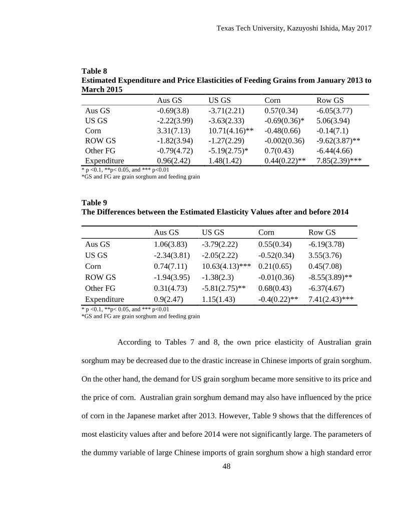
Texas Tech University, Kazuyoshi Ishida, May 2017
48
Table 8 Estimated Expenditure and Price Elasticities of Feeding Grains from January 2013 to March 2015 Aus GS US GS Corn Row GS Aus GS -0.69(3.8) -3.71(2.21) 0.57(0.34) -6.05(3.77) US GS -2.22(3.99) -3.63(2.33) -0.69(0.36)* 5.06(3.94) Corn 3.31(7.13) 10.71(4.16)** -0.48(0.66) -0.14(7.1) ROW GS -1.82(3.94) -1.27(2.29) -0.002(0.36) -9.62(3.87)** Other FG -0.79(4.72) -5.19(2.75)* 0.7(0.43) -6.44(4.66) Expenditure 0.96(2.42) 1.48(1.42) 0.44(0.22)** 7.85(2.39)***
* p <0.1, **p< 0.05, and *** p<0.01 *GS and FG are grain sorghum and feeding grain
Table 9 The Differences between the Estimated Elasticity Values after and before 2014
Aus GS US GS Corn Row GS Aus GS 1.06(3.83) -3.79(2.22) 0.55(0.34) -6.19(3.78) US GS -2.34(3.81) -2.05(2.22) -0.52(0.34) 3.55(3.76) Corn 0.74(7.11) 10.63(4.13)*** 0.21(0.65) 0.45(7.08) ROW GS -1.94(3.95) -1.38(2.3) -0.01(0.36) -8.55(3.89)** Other FG 0.31(4.73) -5.81(2.75)** 0.68(0.43) -6.37(4.67) Expenditure 0.9(2.47) 1.15(1.43) -0.4(0.22)** 7.41(2.43)***
* p <0.1, **p< 0.05, and *** p<0.01 *GS and FG are grain sorghum and feeding grain
According to Tables 7 and 8, the own price elasticity of Australian grain
sorghum may be decreased due to the drastic increase in Chinese imports of grain sorghum.
On the other hand, the demand for US grain sorghum became more sensitive to its price and
the price of corn. Australian grain sorghum demand may also have influenced by the price
of corn in the Japanese market after 2013. However, Table 9 shows that the differences of
most elasticity values after and before 2014 were not significantly large. The parameters of
the dummy variable of large Chinese imports of grain sorghum show a high standard error
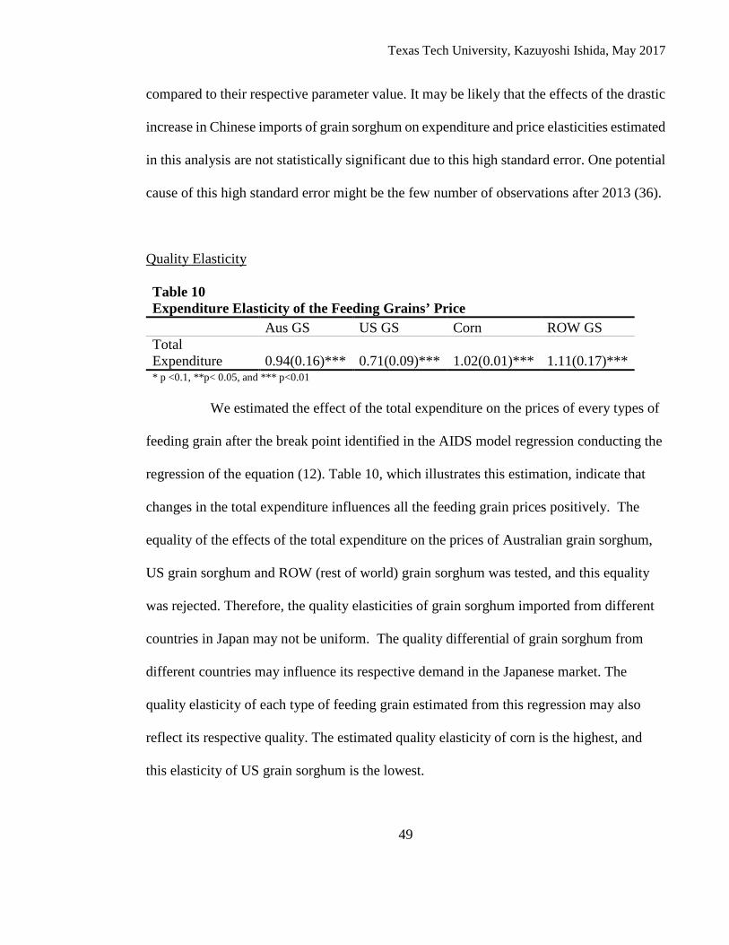
Texas Tech University, Kazuyoshi Ishida, May 2017
49
compared to their respective parameter value. It may be likely that the effects of the drastic
increase in Chinese imports of grain sorghum on expenditure and price elasticities estimated
in this analysis are not statistically significant due to this high standard error. One potential
cause of this high standard error might be the few number of observations after 2013 (36).
Quality Elasticity
Table 10 Expenditure Elasticity of the Feeding Grains’ Price Aus GS US GS Corn ROW GS Total Expenditure 0.94(0.16)*** 0.71(0.09)*** 1.02(0.01)*** 1.11(0.17)*** * p <0.1, **p< 0.05, and *** p<0.01
We estimated the effect of the total expenditure on the prices of every types of
feeding grain after the break point identified in the AIDS model regression conducting the
regression of the equation (12). Table 10, which illustrates this estimation, indicate that
changes in the total expenditure influences all the feeding grain prices positively. The
equality of the effects of the total expenditure on the prices of Australian grain sorghum,
US grain sorghum and ROW (rest of world) grain sorghum was tested, and this equality
was rejected. Therefore, the quality elasticities of grain sorghum imported from different
countries in Japan may not be uniform. The quality differential of grain sorghum from
different countries may influence its respective demand in the Japanese market. The
quality elasticity of each type of feeding grain estimated from this regression may also
reflect its respective quality. The estimated quality elasticity of corn is the highest, and
this elasticity of US grain sorghum is the lowest.
Texas Tech University, Kazuyoshi Ishida, May 2017
50
Random Estimations of the Elasticities
The estimated posterior distributions of the elasticities are displayed in Table 1
in Appendix 2. The mean values of the random estimated elasticities are close to the
elasticity values shown in Table 4. According to Table 1 in Appendix 2, the own price
elasticities of corn, Australian and ROW grain sorghum are negative over the 95% posterior
distribution (from 2.5% to 97.5%).
The posterior distributions of the own price and expenditure elasticities of corn
demand are concentrated on their mean values. This posterior distribution suggests that the
response of the demand for corn to changes in its price and the total expenditure might have
been the same in the Japanese market. On the other hand, the posterior distributions of the
own price elasticity of Australian grain sorghum and its cross price elasticity with corn are
dispersed. Thus, impacts of price changes of corn and Australian grain sorghum on the
demand for Australian grain sorghum might have variations in the Japanese market.
An Analysis of the Effect of the Feed Efficiency using a Bayesian SUR
From the result of the SUR regression using equation (6), the effects of the feed
efficiency on the demand for US and Australian grain sorghum are not clear. A Bayesian
SUR regression of equation (11) was conducted on the data from the breakpoint to 2013
using the following equation. Since the number of the parameters in this equation is large,
this SUR regression is based on the Bayesian analysis. The procedure of the Bayesian SUR
regression is the same as was described previously.
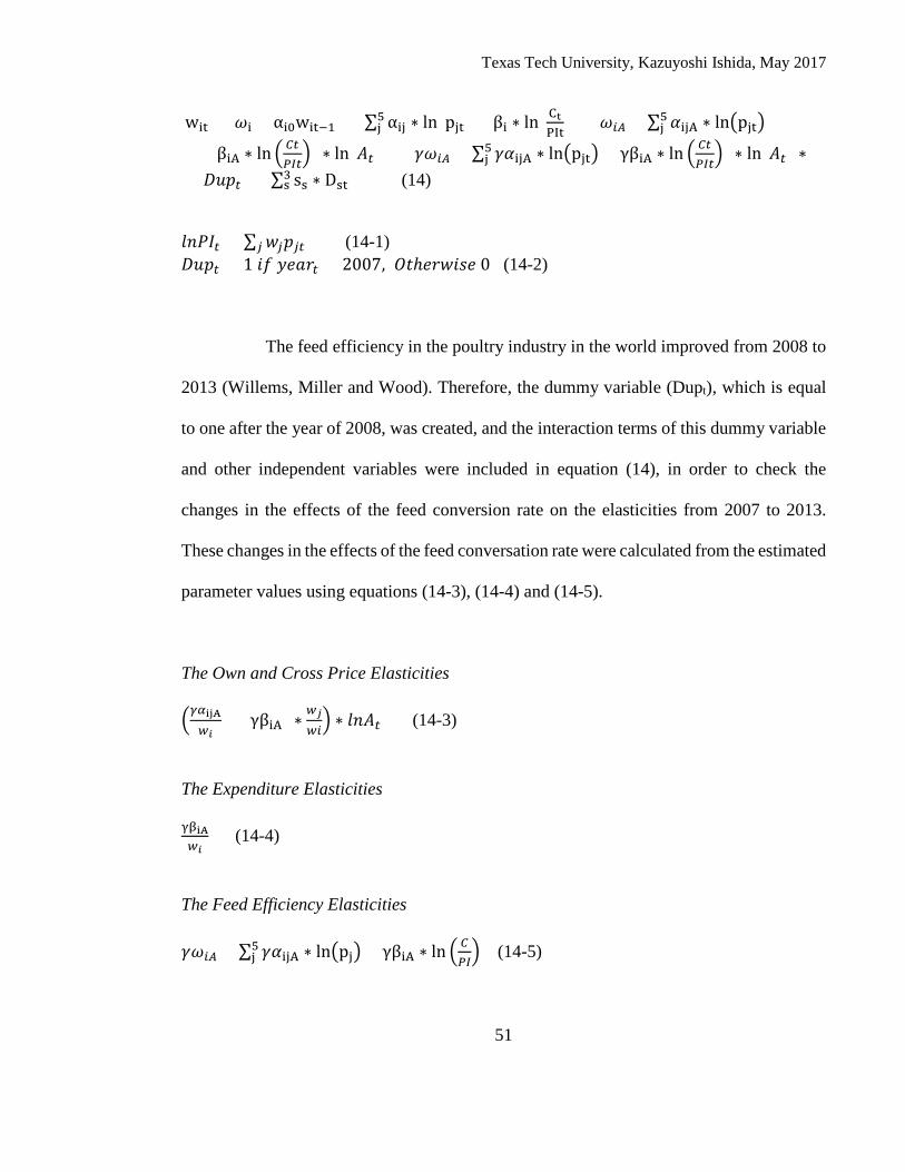
Texas Tech University, Kazuyoshi Ishida, May 2017
51
wit = 𝜔𝜔i + αi0wit−1 + ∑ αij ∗ ln(pjt) + βi ∗ ln ( CtPIt
) + (𝜔𝜔𝑖𝑖𝐴𝐴 + ∑ 𝛼𝛼ijA ∗ lnpjt5j
5j
+βiA ∗ ln 𝐶𝐶𝐶𝐶𝛿𝛿𝑃𝑃𝐶𝐶) ∗ ln (𝐴𝐴𝐶𝐶) + (𝛾𝛾𝜔𝜔𝑖𝑖𝐴𝐴 + ∑ 𝛾𝛾𝛼𝛼ijA ∗ lnpjt5
j + γβiA ∗ ln 𝐶𝐶𝐶𝐶𝛿𝛿𝑃𝑃𝐶𝐶) ∗ ln (𝐴𝐴𝐶𝐶) ∗
𝐷𝐷𝑄𝑄𝑝𝑝𝐶𝐶 + ∑ ss ∗ Dst3s (14)
𝑙𝑙𝑙𝑙𝑃𝑃𝑃𝑃𝐶𝐶 = ∑ 𝑤𝑤𝑗𝑗𝑝𝑝𝑗𝑗𝐶𝐶𝑗𝑗 (14-1) 𝐷𝐷𝑄𝑄𝑝𝑝𝐶𝐶 = 1 𝑄𝑄𝑓𝑓 𝑙𝑙𝑦𝑦𝑄𝑄𝑟𝑟𝐶𝐶 > 2007, 𝑂𝑂𝑄𝑄ℎ𝑦𝑦𝑟𝑟𝑤𝑤𝑄𝑄𝐸𝐸𝑦𝑦 0 (14-2)
The feed efficiency in the poultry industry in the world improved from 2008 to
2013 (Willems, Miller and Wood). Therefore, the dummy variable (Dupt), which is equal
to one after the year of 2008, was created, and the interaction terms of this dummy variable
and other independent variables were included in equation (14), in order to check the
changes in the effects of the feed conversion rate on the elasticities from 2007 to 2013.
These changes in the effects of the feed conversation rate were calculated from the estimated
parameter values using equations (14-3), (14-4) and (14-5).
The Own and Cross Price Elasticities 𝛾𝛾𝛼𝛼ijA
𝑤𝑤𝑖𝑖+ (γβiA) ∗ 𝑤𝑤𝑗𝑗
𝑤𝑤𝑖𝑖 ∗ 𝑙𝑙𝑙𝑙𝐴𝐴𝐶𝐶 (14-3)
The Expenditure Elasticities γβiA𝑤𝑤𝑖𝑖
(14-4) The Feed Efficiency Elasticities 𝛾𝛾𝜔𝜔𝑖𝑖𝐴𝐴 + ∑ 𝛾𝛾𝛼𝛼ijA ∗ lnpj5
j + γβiA ∗ ln 𝐶𝐶𝛿𝛿𝑃𝑃 (14-5)
Texas Tech University, Kazuyoshi Ishida, May 2017
52
Table 2 in Appendix 2 illustrates the posterior distributions of these approximated changes
in the effects of the feed efficiency on the elasticities from 2008 to 2013. According to this
table, the approximated changes in the effects of feed conversion rate on the own-price
elasticity of US grain sorghum over its 95 % posterior distribution are positive.
The upward trend of feeding grain prices might improve feed efficiency in the
Japanese livestock industry. Improvements in the feed efficiency may inflate the negative
effect of a price increase of US grain sorghum on its demand. The result of this analysis
suggests that this inflation might become stronger from 2008 to 2013. As described earlier,
the feed efficiency of poultry feeding leveled up due to increases in prices of feeding grain
in the world from 2008 to 2013. The effect of this feed efficiency improvement on the own
price elasticity of US grain sorghum might become more remarkable over these years in the
Japanese market.
An Analysis of the Effect of Chinese Import of Grain Sorghum using a Bayesian SUR
The previous analysis of the effect of Chinese imports on the demand for US
and Australian grain sorghum didn’t give us a clear result due to the large stand errors.
Therefore, the Bayesian SUR was conducted for identifying this effect. The posterior
distributions of the estimated difference between the elasticities before and after 2014 were
displayed in Table 3 in Appendix 2. This table compared with Table 9, it can be noticed that
the results of this Bayesian SUR and the previous ITSUR have little difference.
The result of this Bayesian SUR also indicates that the difference between the
cross price elasticities of US grain sorghum with corn before and after 2014 is significant
Texas Tech University, Kazuyoshi Ishida, May 2017
53
and positive (this estimated elasticity values over its 95% posterior distribution are
positive). The sudden expansion of Chinse imports of US grain sorghum increase its price
in the Japanese market. On the contrary, the corn price in the Japanese market has been on
the downward trend from January 2013 (Figure 7 in Appendix 2). Decreases in oil prices at
that time led to the contraction of the ethanol demand for corn worldwide. The result of this
regression analysis suggests that the effect of these decreases in the corn price on the
demand for US grain sorghum became large after 2014.
Conclusions
The AIC value of the AIDS model is larger than that of the translog model.
The R-Squares of the AIDS model are also bigger. Therefore, the fitness of the AIDS
model on the data is better. From the result of the regression of the inverse AIDS model,
the effect of the total expenditure on the prices of grain sorghum imported from each
country in the Japanese market is different. Hence, the quality elasticities of grain
sorghum from different countries are not uniform.
After the opening of the futures market of grain sorghum in Australia,
Australian grain sorghum might have become preferable in the Japanese market since
Australian grain sorghum had been produced following the standards specified by its
futures market, and the opening of this futures market might had affected the demand for
Australian grain sorghum and other types of feeding grain in Japan. Hence, this research
identified the structure break points in the elasticity estimations in the translog and AIDS
model. The structure break points of the AIDS and translog model regression are February
Texas Tech University, Kazuyoshi Ishida, May 2017
54
2001 and May 2000, respectively. These identifications of the structure break points
suggest that Australian farmers might have known the opening of the futures market of
grain sorghum in advance, and have started adjusting their production of grain sorghum to
the standards specified in the futures market.
According to the result of the AIDS model regression, the cross price elasticity
of Australian grain sorghum with US grain sorghum is not statistically significant. The
translog model regression estimates that the cross price elasticity of US grain sorghum
with Australian grain sorghum is not statistically significant either. Therefore, an increase
in the price of US grain sorghum may have not affected the quantity demanded of
Australian grain sorghum in the Japanese market. US grain sorghum may have not lost
the market share because this price became more expensive than the price of Australian
grain sorghum.
It might be a possible cause of the loss of this market share that the
substitutability of Australian grain sorghum for corn has become strong in the Japanese
market. Australian grain sorghum was listed in Australian commodity futures market in
2003. From that time, Australian farmers have needed to produce grain sorghum
satisfying the quality standard specified by the future market. As a result, Australian grain
sorghum must have a high standardized quality, and has become strong substitute feeding
grain for corn. Corn price in Japan has risen up recently there due to the corn ethanol
demand and corn’s increased consumption in emerging countries like China. According to
the result of the regression of the AIDS and translog model, this increase in the corn price
may have a positive effect on the demand for Australian grain sorghum. On the other
Texas Tech University, Kazuyoshi Ishida, May 2017
55
hand, the increase in the corn price may not affect the demand for US grain sorghum.
Therefore, though the price of Australian grain sorghum went up in the Japanese market
for the past 10 years, the trend of its consumption was not downward before 2014.
Japanese feed producers may decrease the use of US grain sorghum for their
production of formula feed for improving its feed efficiency, However, the result of the
research using the conventional SUR regression indicate that the effect of the feed
efficiency on the demand of US grain sorghum in the Japanese market is unclear. The feed
efficiency elasticities of US grain sorghum demand estimated from the translog and AIDS
model regressions are not significant due to their large standard error. The result of the
analysis based on the Bayesian SUR regression suggests that the effect of the feed
efficiency on the own-price elasticity of US grain sorghum became stronger after the year
of 2008. From the year of 2008, the feed efficiency of poultry feeding improved
worldwide. This result indicated that this improvement of the feed efficiency might inflate
the negative effect of US grain sorghum price on its demand more after this year.
Since 2014, Chinese demand for grain sorghum has drastically expanded. The
differences of the expenditure and price elasticities of feeding grains before and after the
year of 2014 were estimated using an ITSUR regression. These estimated differences
show that this drastic expansion of Chinese imports may have not affected most of these
elasticities. This regression analysis may be inefficient due to its large standard errors.
Therefore, the differences between the elasticities before and after 2014 were estimated
using a Bayesian SUR model. However, the difference of the estimations of these two
models are small. The estimations from these two econometric model suggest that the
Texas Tech University, Kazuyoshi Ishida, May 2017
56
demand for US grain sorghum may be much more sensitive to the corn price after 2014.
From 2013, the corn price in the Japanese market was on the downward trend, since
decreases in oil prices during that time pushed down the ethanol demand for corn
worldwide. The effect of this downward trend of the corn price have influenced the
demand for US grain sorghum more when Chinese imports of US grain sorghum
expanded drastically. One possible reason is that large amount of Chinese imports of US
grain sorghum lowered the quality of US grain sorghum available in the Japanese market.
Thus, decreases in the corn price have greater impact on the demand for US grain
sorghum in the Japanese market after 2014.
Nowadays, US grain sorghum has no futures market, and hence, US farmers
need not to produce grain sorghum based on certain rigorous specifications. Therefore, the
characteristics of US grain sorghum have a high degree of variability. In other countries
importing US grain sorghum, like Mexico and China, formula feeds may be, in the future,
the main use of livestock feeding. Because of that, it may be desirable for livestock
feeders in these countries to increase the feed efficiency of their livestock feeding. At that
time, grain sorghum with a low quality variability may be preferred, and US grain
sorghum would lose its market share in the world market.
Texas Tech University, Kazuyoshi Ishida, May 2017
57
Reference
Alston, Julian M., Colin A. Carter, Richard Green, and Daniel Pick. "Whither Armington trade models?". American Journal of Agricultural Economics 72, no. 2 (1990): 455-467. Arzac, E. R., & Wilkinson, M.. (1979). A Quarterly Econometric Model of United States Livestock and Feed Grain Markets and Some of Its Policy Implications. American Journal of Agricultural Economics, 61(2), 297–308. Retrieved from http://www.jstor.org/stable/1239734 Armington, P. S. (1969). The Geographic Pattern of Trade and the Effects of Price Changes (Structure géographique des échanges et incidences des variations de prix)(Estructura geográfica del comercio y efectos de la variación de los precios). Staff Papers-International Monetary Fund, 179-201. Australian Stock Exchange. (2016). Contract Specifications. Capehart,T., Allen,E., & Bond,J. (2014). Feed Outlook. USDA Economics Research Service. Christensen, Laurits R., Dale W. Jorgenson, and Lawrence J. Lau. "Transcendental logarithmic utility functions." The American Economic Review 65.3 (1975): 367-383. Chung, C. (2006). Quality bias in price elasticity. Applied Economics Letters, 13(4), 241-245. Cox, T. L., & Wohlgenant, M. K. (1986). Prices and quality effects in cross-sectional demand analysis. American Journal of Agricultural Economics, 68(4), 908-919. Cramer, J. S. (1973). Interaction of income and price in consumer demand. International Economic Review, 351-363. Davis, George C., and Kim L. Jensen. "Two-stage utility maximization and import demand systems revisited: Limitations and an alternative." Journal of Agricultural and resource Economics (1994): 409-424. Food and Agriculture Organization. (2015). FAO STAT. Retrieved from http://faostat3.fao.org/home/E Goldman, S. M., & Uzawa, H. (1964). A note on separability in demand analysis. Econometrica: Journal of the Econometric Society, 387-398.
Texas Tech University, Kazuyoshi Ishida, May 2017
58
Haniotis, T., Baffes, J., & Ames, G. C. (1988). The demand and supply of US agricultural exports: the case of wheat, corn, and soybeans. Southern Journal of Agricultural Economics, 20(02), 45-56. Havenstein, G. B., Ferket, P. R., & Qureshi, M. A. (2003). Growth, livability, and feed conversion of 1957 versus 2001 broilers when fed representative 1957 and 2001 broiler diets. Poultry Science, 82(10), 1500-1508. Honma, M. and Heady, E.O., (1984). An econometric model for international wheat trade: exports, imports, and trade flows. CARD Rep. 124, Ito, Shoichi, Dean T. Chen, and E. Wesley F. Peterson. "Modeling international trade flows and market shares for agricultural commodities: a modified Armington procedure for rice." Agricultural Economics 4, no. 3 (1990): 315-333. Japan Customs. (2016). “Trade Statstics”. retrived from http://www.customs.go.jp/toukei/info/index_e.htm Kazuhiko Kato (2000). "The goal of Improvement of growth of Poultry and Cattle from Japan Minisitry of Agriculture, Forestry and Fishery". Information of Domestic Livestock Industry, (129), 21-26 Lariviere, E., Larue, B., & Chalfant, J. (2000). Modeling the demand for alcoholic beverages and advertising specifications. Agricultural Economics,22(2), 147-162. Lin, W., Allen, G., Ash, M., & Barse, J. R. (1990). Livestock feeds. Seven Farm Input Industries. Agricultural Economic Report, 635, 66-78. Nelson, J. A. (1991). Quality variation and quantity aggregation in consumer demand for food. American Journal of Agricultural Economics, 73(4), 1204-1212. Noguchi, T. (2011). The Present Conditions and Problems of Agricultural Cooperatives for the Feed Grain from the United States and the Formula Feed Supply in Japan, (113), 39-52. Ooe, T. “The supply and demand of US corn and its price settlement mechanism.” Research Reports of Asian Economics Research Institute (2010). Reimer, J. J., Zheng, X., & Gehlhar, M. J. (2012). Export Demand Elasticity Estimation for Major US Crops. Journal of Agricultural and Applied Economics, 44, 501-515.
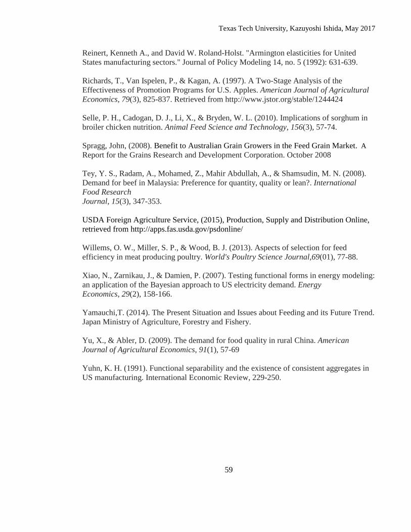
Texas Tech University, Kazuyoshi Ishida, May 2017
59
Reinert, Kenneth A., and David W. Roland-Holst. "Armington elasticities for United States manufacturing sectors." Journal of Policy Modeling 14, no. 5 (1992): 631-639. Richards, T., Van Ispelen, P., & Kagan, A. (1997). A Two-Stage Analysis of the Effectiveness of Promotion Programs for U.S. Apples. American Journal of Agricultural Economics, 79(3), 825-837. Retrieved from http://www.jstor.org/stable/1244424 Selle, P. H., Cadogan, D. J., Li, X., & Bryden, W. L. (2010). Implications of sorghum in broiler chicken nutrition. Animal Feed Science and Technology, 156(3), 57-74. Spragg, John, (2008). Benefit to Australian Grain Growers in the Feed Grain Market. A Report for the Grains Research and Development Corporation. October 2008 Tey, Y. S., Radam, A., Mohamed, Z., Mahir Abdullah, A., & Shamsudin, M. N. (2008). Demand for beef in Malaysia: Preference for quantity, quality or lean?. International Food Research Journal, 15(3), 347-353. USDA Foreign Agriculture Service, (2015), Production, Supply and Distribution Online, retrieved from http://apps.fas.usda.gov/psdonline/ Willems, O. W., Miller, S. P., & Wood, B. J. (2013). Aspects of selection for feed efficiency in meat producing poultry. World's Poultry Science Journal,69(01), 77-88. Xiao, N., Zarnikau, J., & Damien, P. (2007). Testing functional forms in energy modeling: an application of the Bayesian approach to US electricity demand. Energy Economics, 29(2), 158-166. Yamauchi,T. (2014). The Present Situation and Issues about Feeding and its Future Trend. Japan Ministry of Agriculture, Forestry and Fishery. Yu, X., & Abler, D. (2009). The demand for food quality in rural China. American Journal of Agricultural Economics, 91(1), 57-69 Yuhn, K. H. (1991). Functional separability and the existence of consistent aggregates in US manufacturing. International Economic Review, 229-250.
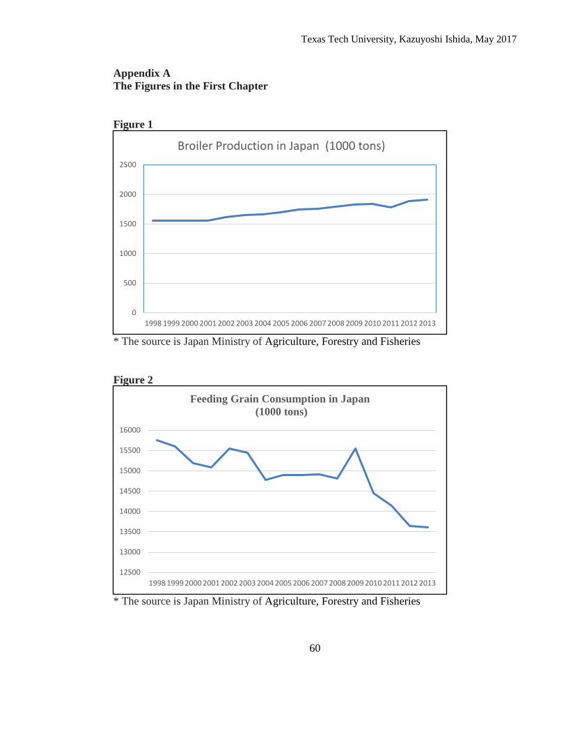
Texas Tech University, Kazuyoshi Ishida, May 2017
60
Appendix A The Figures in the First Chapter Figure 1
* The source is Japan Ministry of Agriculture, Forestry and Fisheries Figure 2
* The source is Japan Ministry of Agriculture, Forestry and Fisheries
0
500
1000
1500
2000
2500
1998 1999 2000 2001 2002 2003 2004 2005 2006 2007 2008 2009 2010 2011 2012 2013
Broiler Production in Japan (1000 tons)
12500
13000
13500
14000
14500
15000
15500
16000
1998 1999 2000 2001 2002 2003 2004 2005 2006 2007 2008 2009 2010 2011 2012 2013
Feeding Grain Consumption in Japan (1000 tons)
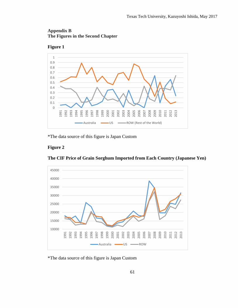
Texas Tech University, Kazuyoshi Ishida, May 2017
61
Appendix B The Figures in the Second Chapter Figure 1
*The data source of this figure is Japan Custom
Figure 2
The CIF Price of Grain Sorghum Imported from Each Country (Japanese Yen)
*The data source of this figure is Japan Custom
00.10.20.30.40.50.60.70.80.9
119
9119
9219
9319
9419
9519
9619
9719
9819
9920
0020
0120
0220
0320
0420
0520
0620
0720
0820
0920
1020
1120
1220
13
Australia US ROW (Rest of the World)
10000
15000
20000
25000
30000
35000
40000
45000
1991
1992
1993
1994
1995
1996
1997
1998
1999
2000
2001
2002
2003
2004
2005
2006
2007
2008
2009
2010
2011
2012
2013
Australia US ROW
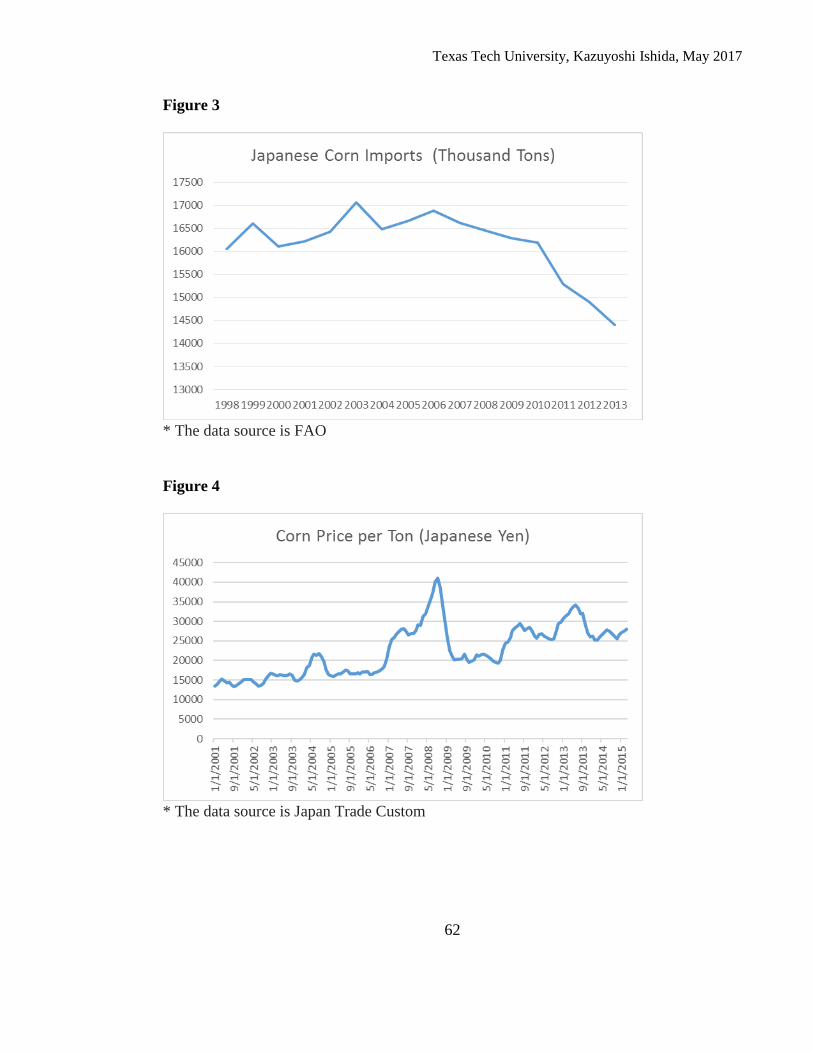
Texas Tech University, Kazuyoshi Ishida, May 2017
62
Figure 3
* The data source is FAO Figure 4
* The data source is Japan Trade Custom
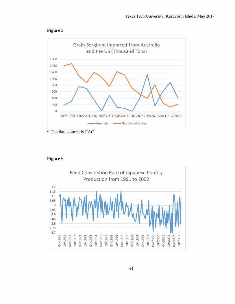
Texas Tech University, Kazuyoshi Ishida, May 2017
63
Figure 5
* The data source is FAO Figure 6
2.72.75
2.82.85
2.92.95
33.05
3.13.15
3.2
04/1
991
10/1
991
04/1
992
10/1
992
04/1
993
10/1
993
04/1
994
10/1
994
04/1
995
10/1
995
04/1
996
10/1
996
04/1
997
10/1
997
04/1
998
10/1
998
04/1
999
10/1
999
04/2
000
10/2
000
04/2
001
10/2
001
04/2
002
10/2
002
Feed Converstion Rate of Japanese Poultry Production from 1991 to 2002
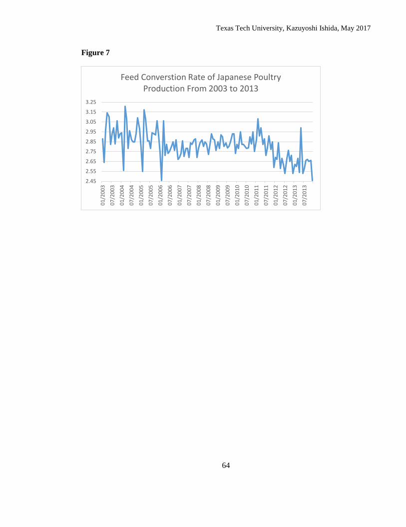
Texas Tech University, Kazuyoshi Ishida, May 2017
64
Figure 7
2.45
2.55
2.65
2.75
2.85
2.95
3.05
3.15
3.2501
/200
3
07/2
003
01/2
004
07/2
004
01/2
005
07/2
005
01/2
006
07/2
006
01/2
007
07/2
007
01/2
008
07/2
008
01/2
009
07/2
009
01/2
010
07/2
010
01/2
011
07/2
011
01/2
012
07/2
012
01/2
013
07/2
013
Feed Converstion Rate of Japanese Poultry Production From 2003 to 2013
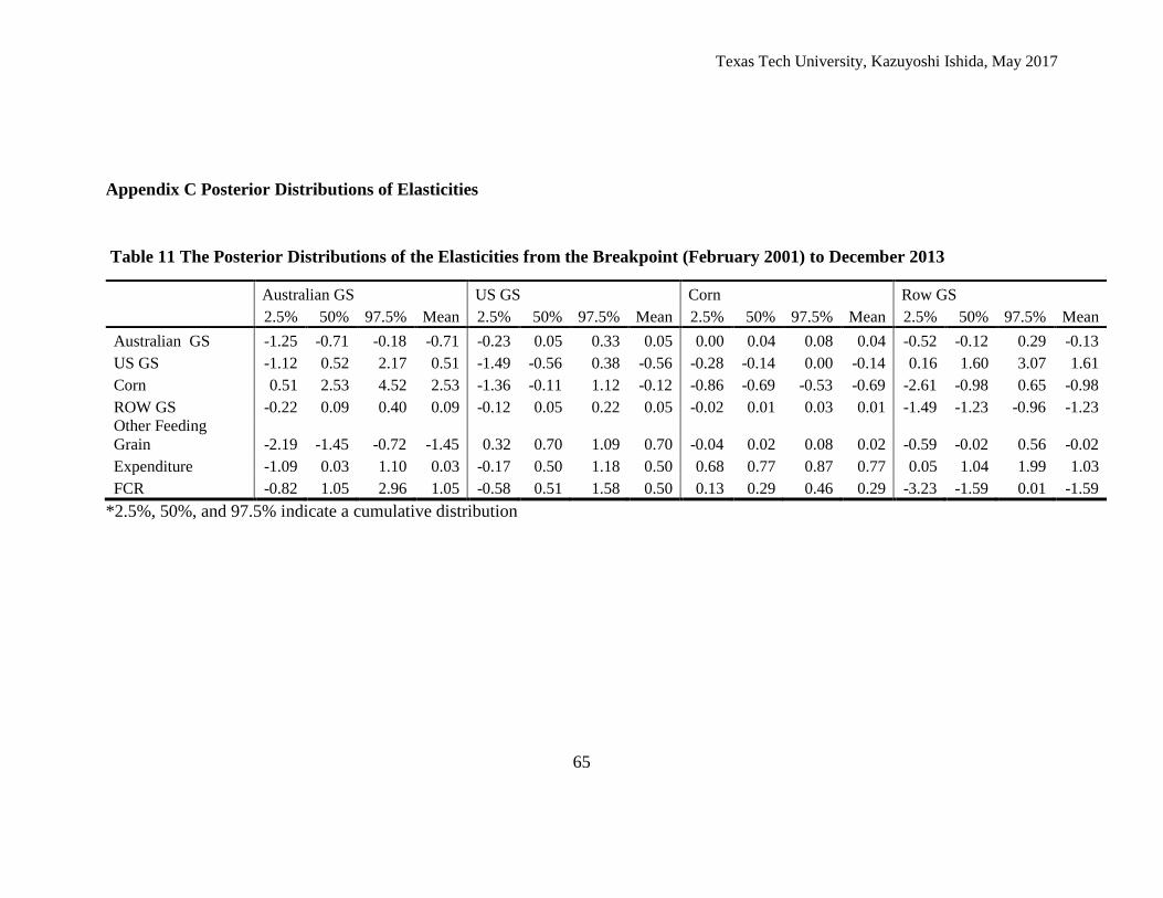
Texas Tech University, Kazuyoshi Ishida, May 2017
65
Appendix C Posterior Distributions of Elasticities
Table 11 The Posterior Distributions of the Elasticities from the Breakpoint (February 2001) to December 2013
Australian GS US GS Corn Row GS 2.5% 50% 97.5% Mean 2.5% 50% 97.5% Mean 2.5% 50% 97.5% Mean 2.5% 50% 97.5% Mean Australian GS -1.25 -0.71 -0.18 -0.71 -0.23 0.05 0.33 0.05 0.00 0.04 0.08 0.04 -0.52 -0.12 0.29 -0.13 US GS -1.12 0.52 2.17 0.51 -1.49 -0.56 0.38 -0.56 -0.28 -0.14 0.00 -0.14 0.16 1.60 3.07 1.61 Corn 0.51 2.53 4.52 2.53 -1.36 -0.11 1.12 -0.12 -0.86 -0.69 -0.53 -0.69 -2.61 -0.98 0.65 -0.98 ROW GS -0.22 0.09 0.40 0.09 -0.12 0.05 0.22 0.05 -0.02 0.01 0.03 0.01 -1.49 -1.23 -0.96 -1.23 Other Feeding Grain -2.19 -1.45 -0.72 -1.45 0.32 0.70 1.09 0.70 -0.04 0.02 0.08 0.02 -0.59 -0.02 0.56 -0.02 Expenditure -1.09 0.03 1.10 0.03 -0.17 0.50 1.18 0.50 0.68 0.77 0.87 0.77 0.05 1.04 1.99 1.03 FCR -0.82 1.05 2.96 1.05 -0.58 0.51 1.58 0.50 0.13 0.29 0.46 0.29 -3.23 -1.59 0.01 -1.59
*2.5%, 50%, and 97.5% indicate a cumulative distribution
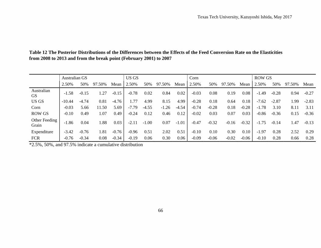
Texas Tech University, Kazuyoshi Ishida, May 2017
66
Table 12 The Posterior Distributions of the Differences between the Effects of the Feed Conversion Rate on the Elasticities from 2008 to 2013 and from the break point (February 2001) to 2007
Australian GS US GS Corn ROW GS 2.50% 50% 97.50% Mean 2.50% 50% 97.50% Mean 2.50% 50% 97.50% Mean 2.50% 50% 97.50% Mean Australian GS -1.58 -0.15 1.27 -0.15 -0.78 0.02 0.84 0.02 -0.03 0.08 0.19 0.08 -1.49 -0.28 0.94 -0.27
US GS -10.44 -4.74 0.81 -4.76 1.77 4.99 8.15 4.99 -0.28 0.18 0.64 0.18 -7.62 -2.87 1.99 -2.83 Corn -0.03 5.66 11.50 5.69 -7.79 -4.55 -1.26 -4.54 -0.74 -0.28 0.18 -0.28 -1.78 3.10 8.11 3.11 ROW GS -0.10 0.49 1.07 0.49 -0.24 0.12 0.46 0.12 -0.02 0.03 0.07 0.03 -0.86 -0.36 0.15 -0.36 Other Feeding Grain -1.86 0.04 1.88 0.03 -2.11 -1.00 0.07 -1.01 -0.47 -0.32 -0.16 -0.32 -1.75 -0.14 1.47 -0.13
Expenditure -3.42 -0.76 1.81 -0.76 -0.96 0.51 2.02 0.51 -0.10 0.10 0.30 0.10 -1.97 0.28 2.52 0.29 FCR -0.76 -0.34 0.08 -0.34 -0.19 0.06 0.30 0.06 -0.09 -0.06 -0.02 -0.06 -0.10 0.28 0.66 0.28
*2.5%, 50%, and 97.5% indicate a cumulative distribution
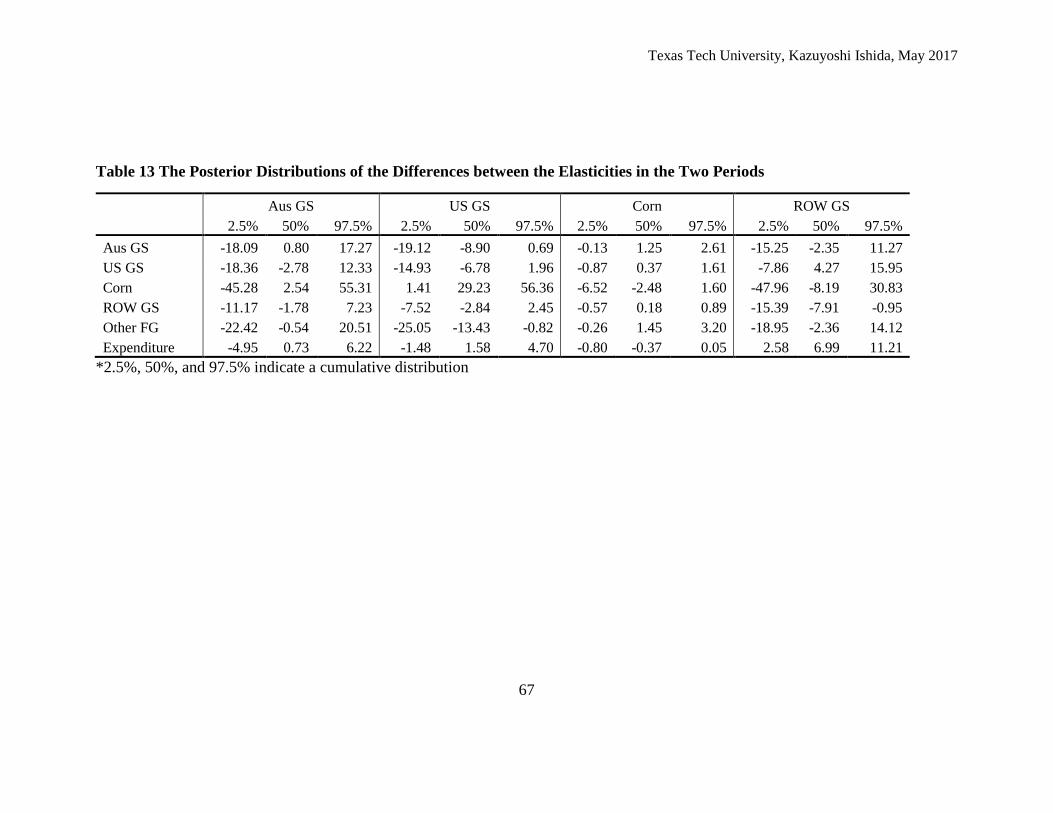
Texas Tech University, Kazuyoshi Ishida, May 2017
67
Table 13 The Posterior Distributions of the Differences between the Elasticities in the Two Periods
Aus GS US GS Corn ROW GS 2.5% 50% 97.5% 2.5% 50% 97.5% 2.5% 50% 97.5% 2.5% 50% 97.5% Aus GS -18.09 0.80 17.27 -19.12 -8.90 0.69 -0.13 1.25 2.61 -15.25 -2.35 11.27 US GS -18.36 -2.78 12.33 -14.93 -6.78 1.96 -0.87 0.37 1.61 -7.86 4.27 15.95 Corn -45.28 2.54 55.31 1.41 29.23 56.36 -6.52 -2.48 1.60 -47.96 -8.19 30.83 ROW GS -11.17 -1.78 7.23 -7.52 -2.84 2.45 -0.57 0.18 0.89 -15.39 -7.91 -0.95 Other FG -22.42 -0.54 20.51 -25.05 -13.43 -0.82 -0.26 1.45 3.20 -18.95 -2.36 14.12 Expenditure -4.95 0.73 6.22 -1.48 1.58 4.70 -0.80 -0.37 0.05 2.58 6.99 11.21
*2.5%, 50%, and 97.5% indicate a cumulative distribution