JID:TCS AID:9587 /FLA Doctopic: Algorithms, automata, complexity and games [m3G; v 1.123; Prn:27/01/2014; 16:27] P.1 (1-15)

Theoretical Computer Science ••• (••••) •••–•••

Contents lists available at ScienceDirect

Theoretical Computer Science

www.elsevier.com/locate/tcs

Upward and quasi-upward planarity testing of embeddedmixed graphs ✩

Carla Binucci a, Walter Didimo a,∗, Maurizio Patrignani b

a Dipartimento di Ingegneria, Università degli Studi di Perugia, Italyb Dipartimento di Ingegneria, Università Roma Tre, Italy

a r t i c l e i n f o a b s t r a c t

Article history:Received 3 April 2012Received in revised form 12 July 2013Accepted 14 January 2014Communicated by J. Kratochvil

Keywords:Graph drawingMixed graphsUpward planarityQuasi-upward planarity

Mixed graphs have both directed and undirected edges and have received considerableattention in the literature. We study two upward planarity testing problems for embeddedmixed graphs, give some NP-hardness results, and describe Integer Linear Programmingtechniques to solve them. Experiments show the efficiency of our approach.

© 2014 Elsevier B.V. All rights reserved.

1. Introduction

1.1. Upward and quasi-upward planarity of directed graphs

An upward drawing of a digraph G is such that all the edges are drawn as curves monotonically increasing in the verticaldirection, according to their orientation. Upward drawings are quite effective to visually convey hierarchical structures, andseveral cognitive experiments demonstrate that the presence of edge crossings in a drawing negatively affects its readabil-ity [31–33]. This scenario has motivated lots of research in the study of the so-called upward planarity testing problem, thatis, the problem of deciding whether a planar digraph admits an upward drawing without edge crossings, also called anupward planar drawing. Figs. 1(a) and 1(b) show a planar digraph G and an upward planar drawing of G .

Bertolazzi et al. [6] proved that if a digraph G with n vertices has a fixed planar embedding, then testing whether Gadmits an upward planar drawing that preserves its embedding can be done in O (n2) time (Fig. 1(b) is a drawing thatpreserves the planar embedding of the digraph in Fig. 1(a)). On the other side, Garg and Tamassia [23] proved that theupward planarity testing problem in the variable embedding setting (i.e., over all planar embeddings of the input digraph) isNP-complete. Several polynomial-time upward planarity testing algorithms have been described in the literature for specificsub-families of planar digraphs [7,18,26,29], and exponential-time upward planarity testing algorithms for more generalcases can be found in [5,13,15,24]. Upward planar drawings with additional properties, called switch-regular, have been alsostudied in [8,17].

We recall that an embedded planar digraph is upward planar only if it is acyclic and bimodal, i.e., for each vertex v allits incoming edges (as well as all its outgoing edges) are consecutive around v . However, acyclicity and bimodality are not

✩ Research supported in part by the MIUR project AMANDA: Algorithmics for MAssive and Networked DAta, prot. 2012C4E3KT_001. An extended abstractof this paper appeared in the proceedings of the 19th International Symposium on Graph Drawing, GD 2011 [9].

* Corresponding author.E-mail addresses: carla.binucci@unipg.it (C. Binucci), walter.didimo@unipg.it (W. Didimo), patrigna@dia.uniroma3.it (M. Patrignani).

0304-3975/$ – see front matter © 2014 Elsevier B.V. All rights reserved.http://dx.doi.org/10.1016/j.tcs.2014.01.015

JID:TCS AID:9587 /FLA Doctopic: Algorithms, automata, complexity and games [m3G; v 1.123; Prn:27/01/2014; 16:27] P.2 (1-15)

2 C. Binucci et al. / Theoretical Computer Science ••• (••••) •••–•••

Fig. 1. (a) A planar digraph G and (b) an upward planar drawing of G . (c) A planar digraph G ′ that is not upward planar and (d) a quasi-upward planardrawing of G ′; edge (5,8) breaks the monotonicity, but still leaves its source from above and enters its target from below.

Fig. 2. (a) A planar embedded mixed graph G . (b) An embedding-preserving planar drawing of G , where the directed edges are drawn upward; the drawingis quasi-upward planar, but not upward planar. (c) An embedding-preserving planar drawing of G where the directed edges are upward and the undirectededges are vertically monotone; the drawing is upward planar.

sufficient conditions for the existence of an upward planar drawing. When a planar digraph has no upward planar drawing,relaxations of the model can be conceived. Bertolazzi et al. introduced the quasi-upward planar drawing convention [5]. In aquasi-upward planar drawing, directed edges are allowed to turn (i.e., to break the vertical monotonicity), but they shouldstill enter vertices from below and leave vertices from above (see Figs. 1(c) and 1(d) for an example). In [5] Bertolazzi et al.prove that a planar embedded digraph admits a quasi-upward planar drawing if and only if it is bimodal (not necessarilyacyclic), and describe a polynomial-time algorithm to compute quasi-upward planar drawings with the minimum numberof edge turns (also called bends) when the planar embedding of the digraph is fixed.

1.2. Upward and quasi-upward planarity of mixed graphs

Many graphs arising from real applications have both directed and undirected edges. These types of graphs are calledmixed graphs and have received considerable attention in the literature (see, e.g., [4,12,14,20,21,28]). Fig. 2(a) shows a mixedgraph whose nodes represent employees of a company; the directed edges describe hierarchical relationships while theundirected edges describe collaborations. In a visual representation of a mixed graph it is still desirable that directed edgesflow upward, as in Fig. 2(b). Additionally, in order to increase the readability of the layout, one may want that even theundirected edges are drawn as vertically monotone curves when possible, as in Fig. 2(c). Indeed, monotone curves have abetter “geodesic tendency”, which is important in comprehending the graph represented by the drawing, as confirmed byhuman cognitive studies [25] and by the interest in a recent visualization paradigm for undirected graphs, called monotonedrawing [1–3].

An upward drawing of a mixed graph G is such that all the directed edges of G are drawn upward and all the undirectededges of G are drawn monotone in the vertical direction.

We address the following main question: Given an embedded planar mixed graph G, does G admit an upward planar drawingthat preserves its planar embedding? The drawing in Fig. 2(c) is an embedding-preserving upward planar drawing of the graphin Fig. 2(a), while the drawing in Fig. 2(b) is not an upward drawing, because edge (Mary, Kate) is not vertically monotone(this edge has two turns). We observe that this problem is equivalent to deciding if there exists an orientation of theundirected edges of G such that the resulting embedded digraph has an upward planar drawing. If such an orientation does

JID:TCS AID:9587 /FLA Doctopic: Algorithms, automata, complexity and games [m3G; v 1.123; Prn:27/01/2014; 16:27] P.3 (1-15)

C. Binucci et al. / Theoretical Computer Science ••• (••••) •••–••• 3

not exist, one can wonder whether the undirected edges can be oriented such that the resulting digraph has a quasi-upwardplanar drawing. In other words, one can search for a quasi-upward planar drawing of the mixed graph, i.e., a drawing suchthat every directed edge (u, v) leaves u from above and enters v from below, and each undirected edge is incident to oneof its end-vertices from below and to the other from above. Fig. 2(b) is an example of a quasi-upward planar drawing ofa mixed graph. Notice that as for digraphs, an upward planar drawing of a mixed graph G is also a quasi-upward planardrawing of G; namely, it can be regarded as a quasi-upward planar drawing with no edge turn.

1.3. Results and structure of the paper

In this paper we study both the upward planarity and the quasi-upward planarity testing problem of mixed graphs, andwe refer to them as the mixed upward planarity and the mixed quasi-upward planarity testing problem, respectively. For theseproblems we describe NP-hardness results, Integer Linear Programming Algorithms, and an experimental analysis of thosealgorithms. More precisely:

• We prove that the mixed quasi-upward planarity testing problem is NP-complete, both in the fixed and in the vari-able embedding setting. We remark that, the quasi-upward planarity testing problem for directed graphs is solvable inpolynomial time in both settings [5].

• We describe ILP (Integer Linear Programming) models both for the mixed quasi-upward planarity testing problem andfor the mixed upward planarity testing problem, in the fixed embedding setting. The latter model is obtained by ex-tending the former; if an upward planar drawing exists, the model allows us to construct one. The number of variablesand constraints of both models is linear in the size of the input graph.

• We present an experimental study that shows how the proposed models can be solved efficiently in practice. Indeed, forall instances of our test suite the computation of a solution takes a few seconds, even for graphs with several hundredsof nodes.

We remark that upward drawings of mixed graphs have been previously addressed by Eiglsperger et al. [20]. Differentlyfrom our results, they describe a heuristic that attempts to compute an upward drawing with few edge crossings. Hence,they do not start from an embedded planar graph, and the final drawing may contain crossings even if the original graphadmits an upward planar drawing according to our definition. We also mention that a relaxation of the quasi-upward planardrawing model for mixed graphs studied here has been recently proposed in [10]; for this alternative model, polynomial-time testing and drawing algorithms are given.

The remainder of the paper is structured as follows. In Section 2 we recall some basic definitions and results aboutupward planar and quasi-upward planar drawings. The NP-hardness results are presented in Section 3. Our ILP models forplanar embedded mixed graphs are described in Section 4. The experimental results are presented in Section 5. Conclusionsand open problems are in Section 6.

2. Definitions and notation

2.1. Bimodal embedded digraphs

Let G be an embedded planar digraph. A source vertex (resp. a sink vertex) of G is a vertex with only outgoing edges(resp. incoming edges). A source vertex or a sink vertex of G is also called a switch vertex of G . A vertex v of G is bimodalif all its incoming edges are consecutive around v (and thus also the outgoing edges are consecutive around v). If allvertices of G are bimodal then G and its embedding are called bimodal. Fig. 3(a) shows an embedded bimodal digraph G .Acyclicity and bimodality are necessary but not sufficient conditions for the upward planar drawability of an embeddedplanar digraph [6]. Note that if G is bimodal, the circular list of edges incident to any vertex v of G can be split into twolinear lists, one consisting of the incoming edges of v and the other consisting of the outgoing edges of v . Namely, thelinear list of the outgoing edges is obtained by scanning them clockwise around v , while the linear list of the incomingedges is obtained by scanning them counterclockwise around v . The first and the last edge in the linear list of incomingedges of v are also called the first incoming edge and the last incoming edge of v , respectively. Similarly, the first outgoing edgeand the last outgoing edge of v refer to the first and to the last edge in the linear list containing the outgoing edges of v .

Let f be a face of G and suppose that the boundary of f is visited clockwise if f is internal, and counterclockwise if fis external. Let a = (e1, v, e2) be a triplet such that v is a vertex of the boundary of f and e1, e2 are two edges incident tov that are consecutive on the boundary of f (e1 and e2 may coincide if G is not biconnected). Triplet a is called an angle atv in face f , or simply an angle of f (see also Fig. 3(a) for an example). An angle a = (e1, v, e2) of a face f is a switch angle off if e1 and e2 are both incoming edges or both outgoing edges of v; otherwise a is a non-switch angle. Angle (e1, v, e2) inFig. 3(a) is a switch angle of f . If v is a switch vertex, all the angles at v are switch angles in the faces incident to v . Wedenote by deg(v) the number of angles at v and by deg( f ) the number of angles in f .

JID:TCS AID:9587 /FLA Doctopic: Algorithms, automata, complexity and games [m3G; v 1.123; Prn:27/01/2014; 16:27] P.4 (1-15)

4 C. Binucci et al. / Theoretical Computer Science ••• (••••) •••–•••

Fig. 3. (a) A planar embedded bimodal digraph G . (b) An angle labeling L of G that is an upward planar embedding of G . (c) An upward planar drawingof G that induces L.

2.2. Upward planar drawings and embeddings

An upward planar drawing of a planar digraph G is a planar drawing of G such that all the edges are drawn as curvesmonotonically increasing in the vertical direction, according to their orientation. Let Γ be an upward planar drawing of anembedded planar digraph G . Assign to each angle a of G a label S , F , or L, according to the following rules: a is labeled Lif it is a switch angle that corresponds to a geometric angle larger than π in Γ ; a is labeled F if it is a non-switch angle;a is labeled S otherwise. Note that an angle is labeled S if it is a switch angle corresponding to a geometric angle smallerthan π in Γ . We call this labeling the upward labeling induced by Γ . Given an embedded bimodal planar digraph G , anassignment L of labels S , F , and L to the angles of G is called an upward planar embedding of G if there exists an upwardplanar drawing Γ of G such that the upward labeling induced by Γ coincides with L. Fig. 3(b) shows an angle labelingL of the embedded digraph in Fig. 3(a): L is an upward planar embedding and Fig. 3(c) shows an upward drawing thatinduces L. For a given angle labeling L and for a given vertex v of G , we denote by L(v), S(v), and F (v) the number ofangles at v that are labeled L, S , and F , respectively; also, if f is a face of G , L( f ), S( f ), and F ( f ) denote the number ofangles of f that are labeled L, S , and F , respectively.

The next theorem characterizes the upward planar embeddings of an embedded bimodal planar digraph G . It is a con-sequence of the results in [18,19].

Theorem 1. Let G be an embedded bimodal planar digraph and let L be an assignment of labels S, F , and L to the angles of G. L is anupward planar embedding of G if and only if the following properties hold:

(a) deg( f ) − 2 = 2L( f ) + F ( f ), for each internal face f of G;(b) deg( f ) + 2 = 2L( f ) + F ( f ), for the external face f of G;(c) Switch angles are labeled either S or L, and non-switch angles are labeled F ;(d) If v is a switch vertex of G then: L(v) = 1, S(v) = deg(v) − 1, F (v) = 0;(e) If v is a non-switch vertex of G then: L(v) = 0, S(v) = deg(v) − 2, F (v) = 2.

Proof. If L is an upward planar embedding of G , then by Theorem 3.2 of [18], properties (c), (d), and (e) are satisfied,in addition to the following: (i) L( f ) = S( f ) − 2 if f is internal; (ii) L( f ) = S( f ) + 2 if f is external. However, sincedeg( f ) = L( f ) + S( f ) + F ( f ), properties (i) and (ii) are equivalent to (a) and (b), as also observed in [19].

Conversely, suppose that L verifies properties (a)–(e). Theorem 3.2 of [18] proves that L is an upward planar embeddingof G , if G is acyclic. In fact, it can be easily proved that G cannot contain directed cycles. Namely, let G ′ be any connectedembedding preserving subgraph of G . Define from L a labeling L′ of the angles of G ′ as follows (see also [18]). Let a =(e1, v, e2) be any angle of G ′ , and let A be the counterclockwise sequence of angles of G at v between e1 and e2. Then:

• a is labeled L if A contains either one angle labeled L or two angles labeled F .• a is labeled F if A contains exactly one angle labeled F .• a is labeled S otherwise.

Lemma 3.3 of [18] shows that L′ still verifies properties (a)–(e), always using the fact that (a) and (b) are equivalent to (i)and (ii). This implies that G cannot contain a directed cycle C , because otherwise letting G ′ = C , and denoted by f theunique internal face of G ′ , it would be L( f ) = S( f ) = 0 in L′ , a contradiction. �

JID:TCS AID:9587 /FLA Doctopic: Algorithms, automata, complexity and games [m3G; v 1.123; Prn:27/01/2014; 16:27] P.5 (1-15)

C. Binucci et al. / Theoretical Computer Science ••• (••••) •••–••• 5

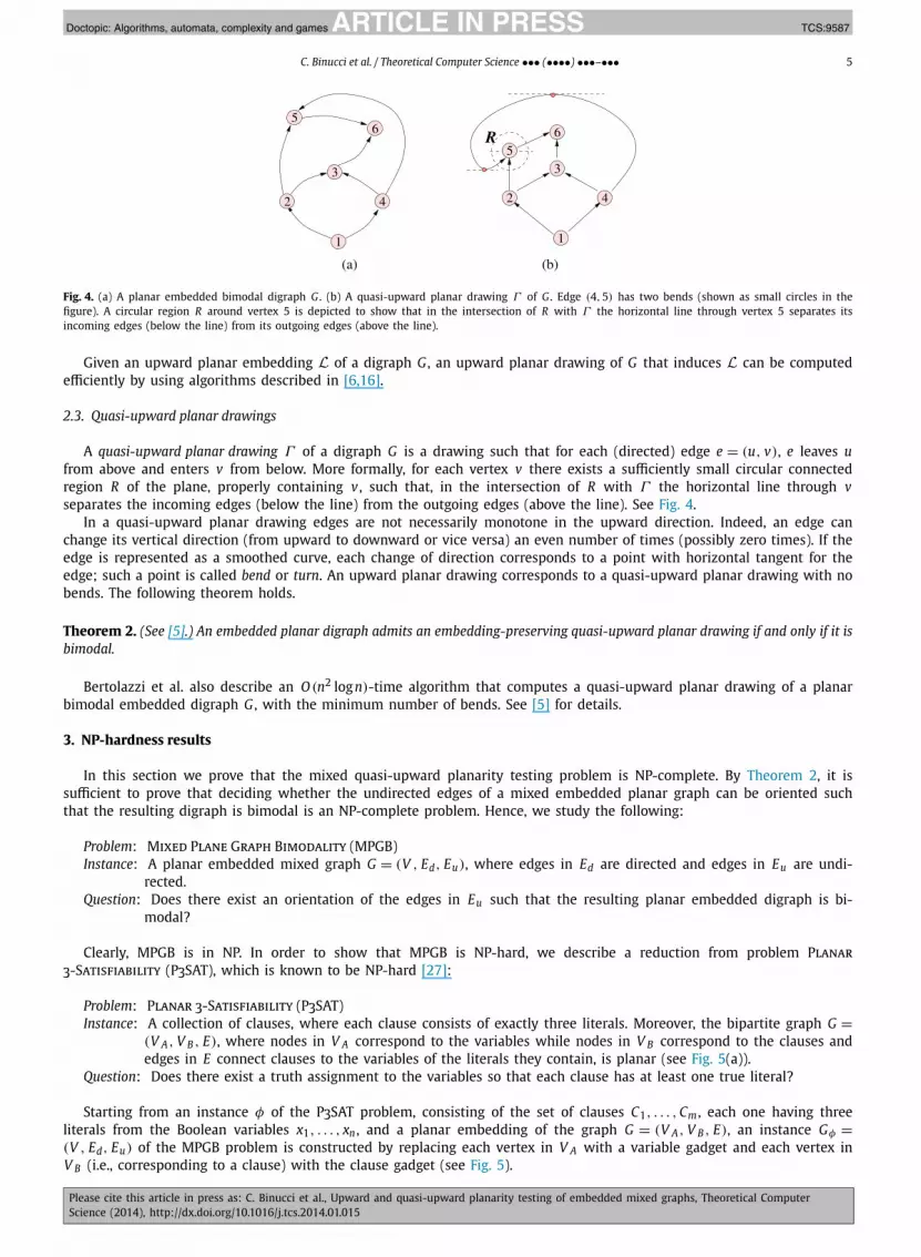
Fig. 4. (a) A planar embedded bimodal digraph G . (b) A quasi-upward planar drawing Γ of G . Edge (4,5) has two bends (shown as small circles in thefigure). A circular region R around vertex 5 is depicted to show that in the intersection of R with Γ the horizontal line through vertex 5 separates itsincoming edges (below the line) from its outgoing edges (above the line).

Given an upward planar embedding L of a digraph G , an upward planar drawing of G that induces L can be computedefficiently by using algorithms described in [6,16].

2.3. Quasi-upward planar drawings

A quasi-upward planar drawing Γ of a digraph G is a drawing such that for each (directed) edge e = (u, v), e leaves ufrom above and enters v from below. More formally, for each vertex v there exists a sufficiently small circular connectedregion R of the plane, properly containing v , such that, in the intersection of R with Γ the horizontal line through vseparates the incoming edges (below the line) from the outgoing edges (above the line). See Fig. 4.

In a quasi-upward planar drawing edges are not necessarily monotone in the upward direction. Indeed, an edge canchange its vertical direction (from upward to downward or vice versa) an even number of times (possibly zero times). If theedge is represented as a smoothed curve, each change of direction corresponds to a point with horizontal tangent for theedge; such a point is called bend or turn. An upward planar drawing corresponds to a quasi-upward planar drawing with nobends. The following theorem holds.

Theorem 2. (See [5].) An embedded planar digraph admits an embedding-preserving quasi-upward planar drawing if and only if it isbimodal.

Bertolazzi et al. also describe an O (n2 log n)-time algorithm that computes a quasi-upward planar drawing of a planarbimodal embedded digraph G , with the minimum number of bends. See [5] for details.

3. NP-hardness results

In this section we prove that the mixed quasi-upward planarity testing problem is NP-complete. By Theorem 2, it issufficient to prove that deciding whether the undirected edges of a mixed embedded planar graph can be oriented suchthat the resulting digraph is bimodal is an NP-complete problem. Hence, we study the following:

Problem: Mixed Plane Graph Bimodality (MPGB)

Instance: A planar embedded mixed graph G = (V , Ed, Eu), where edges in Ed are directed and edges in Eu are undi-rected.

Question: Does there exist an orientation of the edges in Eu such that the resulting planar embedded digraph is bi-modal?

Clearly, MPGB is in NP. In order to show that MPGB is NP-hard, we describe a reduction from problem Planar

3-Satisfiability (P3SAT), which is known to be NP-hard [27]:

Problem: Planar 3-Satisfiability (P3SAT)

Instance: A collection of clauses, where each clause consists of exactly three literals. Moreover, the bipartite graph G =(V A, V B , E), where nodes in V A correspond to the variables while nodes in V B correspond to the clauses andedges in E connect clauses to the variables of the literals they contain, is planar (see Fig. 5(a)).

Question: Does there exist a truth assignment to the variables so that each clause has at least one true literal?

Starting from an instance φ of the P3SAT problem, consisting of the set of clauses C1, . . . , Cm , each one having threeliterals from the Boolean variables x1, . . . , xn , and a planar embedding of the graph G = (V A, V B , E), an instance Gφ =(V , Ed, Eu) of the MPGB problem is constructed by replacing each vertex in V A with a variable gadget and each vertex inV B (i.e., corresponding to a clause) with the clause gadget (see Fig. 5).

JID:TCS AID:9587 /FLA Doctopic: Algorithms, automata, complexity and games [m3G; v 1.123; Prn:27/01/2014; 16:27] P.6 (1-15)

6 C. Binucci et al. / Theoretical Computer Science ••• (••••) •••–•••

Fig. 5. (a) A planar embedding of graph G = (V A , V B , E) for the P3SAT instance φ = (x1 ∨ ¬x2 ∨ x3) ∧ (x2 ∨ ¬x3 ∨ ¬x4) ∧ (¬x1 ∨ x3 ∨ ¬x4) ∧ (x1 ∨ ¬x4 ∨x5) ∧ (x1 ∨ x2 ∨ ¬x5). The black vertices correspond to the clauses. (b) The same instance where variables and clauses are replaced with gadgets.

Fig. 6. (a) A variable gadget. Dashed edges are undirected edges in the input graph. Thick edges are directed edges in the input graph. (b) The variablegadget is true if the edges of the cycle are oriented counter-clockwise in correspondence to sinks (black vertices) and clockwise in correspondence tosources (gray vertices). (c) A false variable gadget.

Namely, for each variable xi of the P3SAT instance we build a variable gadget as depicted in Fig. 6(a). The variable gadgetis composed of a cycle with 2k vertices v0, v1, . . . , v2k−1, where k is the number of occurrences of variable xi in φ, joinedby undirected edges. Also, for each undirected edge ei = (vi, v(i+1) mod k), with i even (odd, respectively), a vertex wi isplaced in the internal portion of the plane and connected with two directed edges (vi, w) and (v(i+1) mod k, w) ((w, vi)

and (w, v(i+1) mod k), respectively). Hence, vertices wi are alternatively sinks (even i) and sources (odd i) in the mixedgraph Gφ . Given an orientation for the undirected edges of Gφ , we say that a variable gadget is true (false, respectively) ifeach edge ei is directed counter-clockwise for even i and clockwise for odd i (clockwise for even i and counter-clockwisefor odd i, respectively). See Figs. 6(b) and 6(c) for examples of true and false variable gadgets.

We have the following lemma.

Lemma 3. In any bimodal orientation of the undirected edges of Gφ , a variable gadget is either true or false.

Proof. Consider edge e0 = (v0, v1) of the variable gadget for a variable x (see Fig. 6(a)). Suppose that in the bimodalorientation e0 is directed counter-clockwise from v0 to v1 as in Fig. 6(b). The direction of the three edges (v0, v1), (v1, w0),and (w1, v1) which are adjacent in the circular list of v1 forces edge e1 to be directed clockwise from v2 to v1 in order forthe orientation to be bimodal. Analogously, the clockwise orientation of e1 and the bimodality of v2 forces edge e2 to bedirected counter-clockwise from v2 to v3. It follows that each ei is directed counter-clockwise when i is even and clockwisewhen i is odd, i.e., the variable gadget is true.

Conversely, suppose that in the bimodal orientation e0 is directed clockwise from v1 to v0 as in Fig. 6(c). Analogousconsiderations allow us to establish that e7 is directed counter-clockwise. In turn, this implies that e6 is directed clockwise,and so on. Hence, in this second case each ei is directed clockwise when i is even and counter-clockwise when i is odd, i.e.,the variable gadget is false. �

JID:TCS AID:9587 /FLA Doctopic: Algorithms, automata, complexity and games [m3G; v 1.123; Prn:27/01/2014; 16:27] P.7 (1-15)

C. Binucci et al. / Theoretical Computer Science ••• (••••) •••–••• 7

Fig. 7. The 2SAT-gadget. If edges e4 and e5 are exiting the 2SAT-gadget, edge e8 is entering it.

A variable gadget is connected to the rest of the graph by attaching undirected edges to the vertices on the externalboundary of it. Regarding the possible orientations of such edges the following lemma holds.

Lemma 4. Consider any bimodal orientation of the undirected edges of Gφ and suppose that the variable gadget for variable x is true.Any edge attached to a vertex vi on the external boundary of the variable gadget is forced to be exiting vi (entering vi , respectively) ifi is even (i is odd, respectively). Conversely, suppose that the variable gadget is false. Any edge attached to a vertex vi on the externalboundary of the variable gadget is forced to be entering vi (exiting vi , respectively) if i is even (i is odd, respectively).

Proof. If the variable gadget is true the edges on its external boundary (thin solid edges of Fig. 6(b)) are directed exitingvertices with even index and entering vertices with odd index. Since each vertex vi is also incident to two internal edgeswhich are directed one entering and one exiting vi (thick solid edges of Fig. 6(b)), in any orientation in which vi is bimodalall additional edges possibly attaching to vi on the external boundary of the variable gadget has to be directed accordingto the direction of the edges of the boundary incident to vi . Analogous considerations hold for the case of a false variablegadget (see Fig. 6(c)), where the vertices of the boundary with odd index play the role of the vertices with even index andvice versa. �

Lemma 4 allows us to associate the truth value encoded by a variable gadget with the direction of the edges attachedto it. Namely, an edge e attached to a vertex vi represents a true value (false value, respectively) if e is oriented exiting vi

(entering vi , respectively). We say that in the two above cases e is true or false. Observe that, if i is even, e encodes thetruth value of a direct literal, whereas if i is odd e encodes the truth value of a negated literal. The edges attached to thevariable gadget for variable x transport the truth values of the literals of x to the clause gadgets.

In order to describe the clause gadget, we first introduce the 2SAT-gadget shown in Fig. 7. The 2SAT-gadget is attachedto the rest of the graph through three edges e4, e5, and e8. Intuitively, the purpose of the 2SAT-gadget is to check if thetruth values encoded in the directions of e4 and e5 are both false, and encode the result in the direction of e8. The maincomponent of the 2SAT-gadget is a cycle of four edges e0, . . . , e3, which forms a construction analogous to that of thevariable gadget (actually, it is a small variable gadget with k = 2). Analogously to the case of the variable gadget, we saythat the 2SAT-gadget is true (false, respectively) if each edge ei is directed counter-clockwise for even i and clockwise forodd i (clockwise for even i and counter-clockwise for odd i, respectively). By Lemma 3, in any bimodal orientation of theundirected edges of Gφ the 2SAT-gadget is either true or false and, consequently, by Lemma 4 edges e6, e7 and e8 are eitherall entering v1 and v3 or all exiting v1 and v3. Edges e4 and e5 are not directly attached to v1. The purpose of vertices z1and z2 and of the edge between them is stated by the following lemma.

Lemma 5. In all bimodal orientations of the undirected edges of the 2SAT-gadget such that edges e4 and e5 are directed exiting z1and z2 , edge e8 is directed entering v3 . Otherwise (e4 and e5 are not both exiting z1 and z2), there exist bimodal orientations of the2SAT-gadget in which e8 has either orientation.

Proof. Suppose that e4 and e5 are directed exiting z1 and z2 (see Fig. 8(a)). Without loss of generality suppose that edge(z1, z2) is directed towards z2. From the bimodality of z2, it follows that e7 is directed entering v1. Lemma 4 implies thate6 is directed entering v1 and e8 is directed entering v3.

Otherwise, suppose that e4 and e5 are directed both entering z1 and z2 (see Fig. 8(b)). Whatever is the orientation ofedge (z1, z2), edges e6 and e7 may be oriented both entering or exiting v1 and, correspondingly, e8 may be oriented exitingor entering v3.

Finally, suppose that e4 and e5 are directed one entering and one exiting z1 and z2 (see Fig. 8(c)). Direct edge (z1, z2)

towards z1. Both the orientations for e6 and e7 are compatible with a bimodal orientation of the 2SAT-gadget and, again,edge e8 may have either orientation. �

JID:TCS AID:9587 /FLA Doctopic: Algorithms, automata, complexity and games [m3G; v 1.123; Prn:27/01/2014; 16:27] P.8 (1-15)

8 C. Binucci et al. / Theoretical Computer Science ••• (••••) •••–•••

Fig. 8. (a) The orientation of the 2SAT-gadget when edges e4 and e5 are exiting the gadget; (b)–(c) any orientation is possible for edge e8 when eitheredges e4 and e5 are oriented entering the gadget or one is entering and one is exiting.

Fig. 9. The clause gadget for MPGB.

The clause gadget is depicted in Fig. 9 and is composed of two 2SAT-gadgets connected together. Observe that edge eTRUEis a directed edge of instance Gφ and that, in particular, it is directed exiting the clause gadget.

The following lemma trivially follows from Lemma 5.

Lemma 6. In any bimodal orientation of the undirected edges of the clause gadget of Fig. 9, at least one among the edges ea, eb , and ec

is directed entering the clause gadget.

Regarding the connections among gadgets, consider the clause gadget for clause C = la ∨ lb ∨ lc and the variable gadgetsfor the corresponding variables xa , xb , and xc . If la is the direct (negated, respectively) literal of variable xa , we attach edgeea of the clause gadget to a vertex v p , with p even (odd, respectively), of the variable gadget for xa . We attach edges eb andec to the variable gadgets of xb and xc in an analogous way.

JID:TCS AID:9587 /FLA Doctopic: Algorithms, automata, complexity and games [m3G; v 1.123; Prn:27/01/2014; 16:27] P.9 (1-15)

C. Binucci et al. / Theoretical Computer Science ••• (••••) •••–••• 9

Lemma 7. The MPGB problem is NP-hard.

Proof. Suppose that the P3SAT instance φ admits a truth assignment such that each clause has at least one true literal.A bimodal orientation for the edges of Gφ can be found as follows. Give to each variable gadget the true or false orientationdepending on the truth value of the corresponding variable. Give to the edges attaching to the variable gadgets the orienta-tion prescribed by Lemma 4. Select one true literal for each clause and orient the corresponding edge of the clause gadgetentering the gadget. It can be seen that the orientation is bimodal.

Conversely, suppose that there exists a bimodal orientation of the edges of Gφ . An assignment of truth values to thevariables x1, x2, . . . , xn satisfying the corresponding P3SAT instance φ can be found as follows. From the orientation of eachvariable gadget a truth value for the corresponding variable can be obtained. The true literal of each clause can be obtainedby observing the direction of the edges of the corresponding clause gadget.

As the construction of the MPGB instance Gφ corresponding to φ can be done in polynomial time, the statement fol-lows. �

We remark that the fixed embedding hypothesis is not strictly needed for the statement of Lemma 7 to hold. In par-ticular, some edges and vertices can be suitably added to Gφ in order to obtain a graph G ′

φ that admits a single planarembedding (up to a flip), implying the NP-hardness of MPGB also in the variable embedding setting. Namely, for each facef of G with more than three vertices, we insert into f a vertex v f and join each vertex vi on the boundary of f to v fwith a path of length two composed by one undirected edge (vi, v ′

i) and one directed edge (v ′i, v f ). Since the obtained

graph G ′φ is a subdivision of a triconnected graph, it admits a single embedding. Further, G ′

φ admits a bimodal orientationif and only if Gφ does. In fact, a bimodal orientation of G ′

φ implies a bimodal orientation of its subgraph Gφ . Conversely,a bimodal orientation of Gφ can be extended to a bimodal orientation of G ′

φ by orienting the undirected edges (vi, v ′i) in

such a way to maintain vi bimodal. Details can be found in [30].From Theorem 2, Lemma 7, and from the fact that MPGB is in NP, the following holds.

Theorem 8. The mixed quasi-upward planarity testing problem is NP-complete.

4. Integer Linear Programming models

Let G be an embedded planar mixed graph. In this section we describe Integer Linear Programming (ILP) models for themixed quasi-upward planarity testing problem and for the mixed upward planarity testing problem, in the fixed embeddingsetting. The second model is obtained by suitably extending the first one.

4.1. ILP model for the mixed quasi-upward planarity testing problem

By Theorem 2, a quasi-upward planar drawing of G exists if and only if we are able to find an orientation of theundirected edges of G such that the resulting digraph G ′ is a bimodal embedded digraph. If G ′ is found, an embeddingpreserving quasi-upward planar drawing of G ′ can be computed with the polynomial-time algorithm described in [5]. Todecide whether G ′ exists we define an ILP model, whose sets, variables, and constraints are described below. Clearly, weassume that the embedded digraph obtained from G by removing all the undirected edges is bimodal, otherwise we canimmediately conclude that G ′ does not exist.

4.1.1. Sets and variablesLet V denote the set of vertices of G and E the set of edges of G . Set E is partitioned into two subsets Ed and Eu ,

containing the directed and the undirected edges of G , respectively. For each vertex v ∈ V , the set of angles at v is denotedas A(v). The set of all angles is denoted by A.

We associate a binary variable �a with each angle a = (e1, v, e2). If �a = 0, angle a will be a switch angle (i.e., e1 and e2will be both outgoing or both incoming edges of v). If �a = 1, angle a will be a non-switch angle.

For each edge e = (u, v) we define two binary variables, ouv and ovu , which describe the orientation of e in G ′; if ouv = 1edge e is oriented from u to v , otherwise it is oriented from v to u.

Finally, for each angle a = (e1, v, e2), we define a binary variable ca . This variable is used to guarantee consistencybetween the orientations of e1, e2 and the value of �a , as explained later.

4.1.2. ConstraintsConsistency about the orientations of the edges is ensured by Constraint (1): The first constraint forces the directed

edges of G to keep their orientation in G ′ , and the second avoids that an edge could receive two distinct orientations at thesame time.

ouv = 1, ∀(u, v) ∈ E D , ouv + ovu = 1, ∀(u, v) ∈ E. (1)

JID:TCS AID:9587 /FLA Doctopic: Algorithms, automata, complexity and games [m3G; v 1.123; Prn:27/01/2014; 16:27] P.10 (1-15)

10 C. Binucci et al. / Theoretical Computer Science ••• (••••) •••–•••

The next constraint guarantees consistency between the value of a variable �a and the type of angle a (switch or non-switch), according to our convention. In the constraint v1 denotes the end-vertex of e1 other than v and v2 denotes theend-vertex of e2 other than v .

ov v1 + ov v2 = �a + 2ca, ∀a = (e1, v, e2) ∈ A. (2)

Indeed, if e1 and e2 are both incoming edges of v , then ov v1 + ov v2 = 0, which implies ca = 0 and �a = 0. If e1 and e2are both outgoing edges of v , then ov v1 + ov v2 = 2, which implies ca = 1 and �a = 0. Finally, if e1 and e2 are one incomingand one outgoing, then ov v1 + ov v2 = 1, which implies ca = 0 and �a = 1. Hence, Constraint (2) implies that �a = 0 if a is aswitch angle and �a = 1 if a is a non-switch angle.

Finally, an embedded digraph is bimodal if and only if the number of non-switch angles at each vertex is either 0or 2. Indeed, in any embedded planar digraph the number of non-switch angles at any vertex is an even number (possiblyzero), and if a vertex is not bimodal it has at least 4 non-switch angles. Hence, we add the following further constraint toguarantee bimodality.

∑

a∈A(v)

�a � 2, ∀v ∈ V . (3)

Note that Constraint (3) by itself does not avoid that∑

a∈A(v) �a = 1. However, since the number of non-switch angles atany vertex is an even number, and since, by Constraint (2), �a = 1 iff a is a non-switch angle, this situation cannot happen.

We observe that the total number of variables and constraints of our model is linear in the number of angles and edgesof G; therefore, since G is planar, it is linear in the number of vertices of G . The following lemma holds.

Lemma 9. There exists an ILP model to decide if a planar embedded mixed graph admits an orientation for its undirected edges suchthat the resulting embedded digraph is bimodal. The number of variables and constraints of the model is linear in the number of verticesof the graph.

By Lemma 9 and by Theorem 2, we have the following theorem.

Theorem 10. There exists an ILP model to decide if a planar embedded mixed graph admits a quasi-upward planar drawing. Thenumber of variables and constraints of the model is linear in the number of vertices of the graph.

4.2. ILP model for the mixed upward planarity testing problem

In order to decide whether an embedded planar mixed graph G admits an upward planar drawing, we use the charac-terization of Theorem 1. Namely, we want to find an orientation for the undirected edges of G and a labeling L for theangles of G such that the resulting digraph is bimodal and L is an upward planar embedding of this embedded digraph.G ′ will denote the digraph obtained from G by orienting its undirected edges. To decide whether G ′ and L exist we definean ILP model that enhances that of Section 4.1 with additional sets, variables, and constraints, as described below. For anillustration of the ILP model, see also Fig. 10. Again, we assume that the embedded digraph obtained from G by removing allthe undirected edges is bimodal, otherwise we can immediately conclude that G does not have an upward planar drawing.

4.2.1. Sets and variablesLet V , E , F , and A denote the set of vertices, edges, faces, and angles of G , respectively.We still partition E into two subsets Ed and Eu , containing the directed and the undirected edges of G , respectively.Set V is partitioned into two subsets V NS and V PS . Each vertex in V NS has both incoming and outgoing edges, and

therefore it cannot be a switch vertex of G ′ . Subset V PS contains the remaining vertices of V ; each element in V PS is apotential switch vertex of G ′ .

Set A is partitioned into two subsets ANS and APS , which contain the angles of G at vertices in V NS and in V PS , respec-tively. For a vertex v and for a face f , A(v) and A( f ) denote all angles at v and all angles in f , respectively. For a vertexv ∈ V NS , ANS(v) is the set of angles at v . For a vertex v ∈ V PS , APS(v) is the set of angles at v . If v ∈ V NS , we denote by e′

outand e′′

out the first and the last outgoing edge of v , respectively (e′out and e′′

out may coincide). Analogously, e′in and e′′

in are thefirst and the last incoming edges of v . The set of angles at v formed by the edges between e′

in and e′out in clockwise order

is denoted by AlNS(v). The set of angles at v formed by the edges between e′′

in and e′′out in counterclockwise order is denoted

by ArNS(v). The set of the remaining angles at v is denoted by Am

NS(v).We associate a variable �a with each angle a = (e1, v, e2). Variable �a takes values 0, 1, or 2, which correspond to the

labels S , F , or L for a, respectively.For each edge e = (u, v) we still define the two binary variables ouv and ovu , which define the orientation of e in G ′; if

ouv = 1 edge e is oriented from u to v , otherwise it is oriented from v to u.Finally, for each angle a = (e1, v, e2), we define a variable ca that takes values in the set {−1,0,1}. This variable is used

to guarantee consistency between the orientations of e1, e2 and the value of �a , as explained later.

JID:TCS AID:9587 /FLA Doctopic: Algorithms, automata, complexity and games [m3G; v 1.123; Prn:27/01/2014; 16:27] P.11 (1-15)

C. Binucci et al. / Theoretical Computer Science ••• (••••) •••–••• 11

Fig. 10. (a) A mixed graph G = (V , E). Set V PS = {0,1,2,4,6,7,8,9,10,11,12,13,14}, set V NS = {3,5}. Set E D = {1,2,3,4,7,10,13,15,16,17,20,23,25},set EU = {5,6,8,9,11,12,14,18,19,21,22,24,26}. Consider, for example, vertex 0 ∈ V PS: APS(0) = {(4,0,24), (24,0,25), (25,0,4)} and adj(v) ={1,2,14}. For vertex 3 ∈ V NS , we have e′

out = e′′out = 20, e′

in = 17, e′′in = 15, Al

NS(3) = {(21,3,17), (20,3,21)}, ArNS(3) = {(15,3,5), (5,3,20)}

and AmNS(3) = {(7,3,15), (18,3,7), (17,3,18)}. For vertex 5 ∈ V NS , e′

out = e′′out = 10, e′

in = e′′in = 13, Al

NS(5) = {(13,5,11), (10,5,11)}, ArNS(5) =

{(13,5,6), (6,5,14), (14,5,10)} and AmNS(3) = ∅. Consider, for example, the internal face f . Then A( f ) = {(18,3,7), (7,4,6), (6,5,14), (14,9,18)} and

cap( f ) = 2. (b) An orientation for the undirected edges of G and an upward planar embedding L of G computed by the ILP model. (c) An upward planardrawing of G that induces L.

4.2.2. ConstraintsWe must guarantee bimodality and the properties of Theorem 1. As for the model presented in Section 4.1, consistency

about the orientation of the edges is ensured by the following constraints.

ouv = 1, ∀(u, v) ∈ E D , ouv + ovu = 1, ∀(u, v) ∈ E. (4)

Also, for each angle a = (e1, v, e2) we have to guarantee consistency between its label and the orientation of the edgese1 and e2. Namely, denote by v1 the vertex of e1 other than v , and denote by v2 the vertex of e2 other than v . If ov v1 andov v2 have the same value (which means that e1 and e2 are both incoming or both outgoing v) then �a must take a value in{0,2}. Otherwise, �a must take value 1. This property is forced by the following constraint:

ov v1 + ov v2 = �a + 2ca, ∀a = (e1, v, e2) ∈ A. (5)

Indeed, as for Constraint (2), if ov v1 + ov v2 is 0 or 2, then �a must be an even number, hence it equals 0 or 2; namely,�a = 0 for ca = 0 or ca = 1, while �a = 2 for ca = −1 or ca = 0. Conversely, �a must be equal to 1 if ov v1 + ov v2 = 1, whichimplies ca = 0.

For an internal face (resp. the external face) f of G , denote by cap( f ) the number of angles in f minus 2 (resp. plus 2).Properties (a) and (b) are guaranteed by the following constraints:

∑

a∈A( f )

�a = cap( f ), ∀ f ∈ F . (6)

Properties (c)–(e) and bimodality are guaranteed by Constraints (7) and (8).∑

a∈APS(v)

�a = 2, ∀v ∈ V PS, (7)

∑

a∈AlNS(v)

�a = 1,∑

a∈ArNS(v)

�a = 1,∑

a∈AmNS(v)

�a = 0, ∀v ∈ V NS. (8)

We finally observe that Constraint (5) and the integrality constraints on variables ouv and ca , imply that variables �a

always assume integer values. Hence, we can relax the integrality constraints on �a , by simply requiring that 0 � �a � 2.The total number of variables and constraints of this model is still linear in the number of angles and edges of G;

therefore, since G is planar, it is linear in the number of vertices of G . The next theorem summarizes the main contributionof this section.

Theorem 11. There exists an ILP model to decide if a planar embedded mixed graph admits an upward planar embedding, and to findone in the positive case. The number of variables and constraints of the model is linear in the number of vertices of the graph.

JID:TCS AID:9587 /FLA Doctopic: Algorithms, automata, complexity and games [m3G; v 1.123; Prn:27/01/2014; 16:27] P.12 (1-15)

12 C. Binucci et al. / Theoretical Computer Science ••• (••••) •••–•••

5. Experimental study

We implemented our ILP models using the AMPL mathematical language1 and ran the computations with the CPLEXsolver,2 using its default setting. We experimented the ILP computations on a large set of mixed graphs in order to under-stand if they are computationally feasible in practice. We focused on two major issues:

Issue 1: What is the time required to find an upward (resp. a quasi-upward) planar embedding of an embedded mixedgraph, if one exists?

Issue 2: What is the time required to decide whether a mixed graph admits an upward (resp. a quasi-upward) planarembedding?

To this aim, we ran the experiments on two different test suites of mixed graphs, which we refer to as MixedPositive

and MixedGeneral. MixedPositive contains mixed embedded planar graphs that always admit an embedding-preservingupward planar drawing. Hence, for these graphs the computation of any of the two ILP models never rejects the instance,and we can measure the time required to find an upward (resp. a quasi-upward) planar embedding. MixedGeneral containsmixed embedded planar graphs for which an upward or a quasi-upward planar drawing may or may not exist. From theexperiments we expect that:

Hypothesis 1: The computation of both ILP models is reasonably fast, as the number of variables and constraints is linearin the size of the graph and most constraints can be also translated into a network flow model.

Hypothesis 2: The computation is faster on those instances that do not admit a solution; indeed, in these cases we expectthat the solver is able to verify, within an initial short time, that some constraints cannot be respected, and as aconsequence that the instance is “quickly” rejected.

Hypothesis 3: On the positive instances the time required to find an embedding increases not only with the size (verticesand density) of the graph, but also when the number of undirected edges increases. This is because for all theseedges a consistent orientation must be found.

Each graph G in MixedPositive was generated by first generating an upward planar embedded digraph G ′ with thealgorithm described in [16], and then removing the orientation on a certain percentage of edges of G ′ . The edges that aremade undirected were selected randomly with a uniform probability distribution. Each graph was generated independentlyof the others.

Each graph G in MixedGeneral was generated with the following procedure: Again, we first generated an upward pla-nar embedded digraph G ′ with the algorithm in [16]. Then a planar embedded mixed graph was computed from G ′ byrepeating the following steps until the desired percentage of undirected edges was reached: Randomly choose a face f ofG ′ and add an edge in f randomly selecting its end-vertices (multiple edges are avoided); then randomly remove from G ′ adirected edge, while maintaining the connectivity. Every random choice followed a uniform probability distribution. As forthe MixedPositive graphs, each graph in MixedGeneral was generated independently of the others.

Set MixedPositive contains 3 graphs for each distinct triple 〈n,d, p〉, where n ∈ {100,200, . . . ,800} is the number ofvertices, d ∈ {1.4,1.6,1.8,2} is the density, and p ∈ {20,50,80} is the percentage of undirected edges of the graph. Hence,MixedPositive contains 288 graphs in total. Set MixedGeneral contains 10 graphs for each distinct triple 〈n,d, p〉, where n,d, and p take the same values as before. Thus, it contains 960 graphs in total.

The experiments were performed under the Windows Vista OS on a PC with an Intel Core-Duo 2.2 GHz processor and2 GB of RAM. These experiments confirmed all our hypotheses. Namely:

• The computations were rather fast and, as expected, the CPU time for the graphs in MixedPositive increased when thesize of the graphs and the percentage of undirected edges increased. This behavior is reported in the charts of Fig. 11,where we show separately the average values on two groups of density, 1.4–1.6 and 1.8–2. The small peaks in fewsamples (e.g., the samples with 600 vertices and 80% of undirected edges) are caused by few instances that made thesolver computation slightly harder. In particular, for the upward planarity testing there was a graph with 600 vertices,80% of undirected edges, and density 2 for which the computation required 12 seconds; for almost all other instancesthe computations took less than 4 seconds.

• Concerning the upward planarity testing of graphs in MixedGeneral, the percentage of negative instances (i.e., thepercentage of graphs for which an upward planar embedding does not exist) is close to 100% for most graphs with 20%or 50% of undirected edges. For the instances with 80% of undirected edges, the number of those that admit a solutiondecreases with the size of the graph (vertices and density): about 88% of the instances with density 1.4–1.6 admit asolution, while this percentage is reduced to 40% for the instances with density 1.8–2 (see Figs. 12(a) and 12(b)). Asexpected, the computation is very fast on the negative instances (each of these instances was rejected within 1 second),

1 http://www.ampl.com/.2 http://www.cplex.com/.

JID:TCS AID:9587 /FLA Doctopic: Algorithms, automata, complexity and games [m3G; v 1.123; Prn:27/01/2014; 16:27] P.13 (1-15)

C. Binucci et al. / Theoretical Computer Science ••• (••••) •••–••• 13

Fig. 11. CPU time for the graphs in MixedPositive: (a)–(b) the values for the computations of the ILP model for upward planarity testing; (c)–(d) the valuesfor the computations of the ILP model for quasi-upward planarity testing. For each of the two groups of density, the values are averaged over all graphswith the same number of vertices and with the same percentage of undirected edges.

Fig. 12. Results for the upward planarity testing computations on the MixedGeneral graphs: (a)–(b) percentage of negative instances. (c)–(d) CPU time. Foreach of the two groups of density, the values are averaged over all graphs with the same number of vertices and with the same percentage of undirectededges.

while the behavior on the positive instances reflects the one for the graphs in MixedPositive (see Figs. 12(c) and 12(d)).In particular, observe the behavior of the running time on the instances with 80% of undirected edges. This timebecomes close to zero for the graphs with 800 vertices and densities 1.8–2, due to a significant increase of the negativeinstances. On the other side, the running time for the graphs with 800 vertices and densities 1.4–1.6 tends to increase

JID:TCS AID:9587 /FLA Doctopic: Algorithms, automata, complexity and games [m3G; v 1.123; Prn:27/01/2014; 16:27] P.14 (1-15)

14 C. Binucci et al. / Theoretical Computer Science ••• (••••) •••–•••

Fig. 13. Results for the quasi-upward planarity testing computations on the MixedGeneral graphs: (a)–(b) percentage of negative instances. (c)–(d) CPUtime. For each of the two groups of density, the values are averaged over all graphs with the same number of vertices and with the same percentage ofundirected edges.

with respect to instances with 600 and 700 vertices, because the number of negative instances remains constant. Finally,observe that the computations on the graphs with 80% of undirected edges are faster on the graphs with higher density(1.8–2); this is still motivated by the fact that most of these graphs are negative instances, which are quickly rejectedby the solver.

• For the quasi-upward planarity testing of graphs in MixedGeneral, the percentage of negative instances (i.e., the per-centage of graphs for which a bimodal embedding does not exist) is clearly much smaller than for the upward planaritytesting. In particular, almost all graphs with 80% of undirected edges are quasi-upward planar (see Figs. 13(a) and 13(b)).Again, the behavior of the running time on the positive instances reflects the one for the graphs in MixedPositive (seeFigs. 13(c) and 13(d)).

6. Conclusions and open problems

We introduced new upward and quasi-upward planarity testing problems for embedded mixed graphs and we ex-perimentally showed that these problems can be efficiently solved using Integer Linear Programming. We conclude bymentioning two main open problems that are concerned with our results:

• What is the theoretical computational complexity of the upward planarity testing problem for planar embedded mixedgraphs? Frati et al. recently proved that this problem is polynomially-time solvable for restricted classes of graphs [22],and we were only able to show that the mixed quasi-upward planarity testing problem in the fixed embedding settingis NP-hard. It is also worth recalling that the upward planarity testing problem for embedded digraphs is polynomi-ally solvable [6] and that polynomial-time algorithms exist for finding upward embeddings of embedded undirectedgraphs [19].

• The design of algorithms for computing the maximum upward planar subgraph of embedded mixed graphs is also aninteresting research direction. We recall that the problem of computing a maximum upward planar subgraph of a planarembedded digraph is NP-hard [11].

Acknowledgements

We wish to thank the anonymous reviewers for their valuable comments, which helped us to improve the quality of thepaper.

JID:TCS AID:9587 /FLA Doctopic: Algorithms, automata, complexity and games [m3G; v 1.123; Prn:27/01/2014; 16:27] P.15 (1-15)

C. Binucci et al. / Theoretical Computer Science ••• (••••) •••–••• 15

References

[1] P. Angelini, E. Colasante, G.D. Battista, F. Frati, M. Patrignani, Monotone drawings of graphs, J. Graph Algorithms Appl. 16 (1) (2012) 5–35.[2] P. Angelini, W. Didimo, S. Kobourov, T. Mchedlidze, V. Roselli, A. Symvonis, S. Wismath, Monotone drawings of graphs with fixed embedding, Algorith-

mica (2013), http://dx.doi.org/10.1007/s00453-013-9790-3.[3] P. Angelini, W. Didimo, S.G. Kobourov, T. Mchedlidze, V. Roselli, A. Symvonis, S.K. Wismath, Monotone drawings of graphs with fixed embedding, in:

Graph Drawing, in: Lect. Notes Comput. Sci., vol. 7034, Springer, 2011, pp. 379–390.[4] J. Bang-Jensen, G. Gutin, Digraphs: Theory, Algorithms and Applications, 2nd edition, Springer, 2009.[5] P. Bertolazzi, G. Di Battista, W. Didimo, Quasi-upward planarity, Algorithmica 32 (3) (2002) 474–506.[6] P. Bertolazzi, G. Di Battista, G. Liotta, C. Mannino, Upward drawings of triconnected digraphs, Algorithmica 6 (12) (1994) 476–497.[7] P. Bertolazzi, G. Di Battista, C. Mannino, R. Tamassia, Optimal upward planarity testing of single-source digraphs, SIAM J. Comput. 27 (1998) 132–169.[8] C. Binucci, E. Di Giacomo, W. Didimo, A. Rextin, Switch-regular upward planar embeddings of directed trees, J. Graph Algorithms Appl. 15 (5) (2011)

587–629.[9] C. Binucci, W. Didimo, Upward planarity testing of embedded mixed graphs, in: Graph Drawing, in: Lect. Notes Comput. Sci., vol. 7034, 2012,

pp. 427–432.[10] C. Binucci, W. Didimo, Quasi-upward planar drawings of mixed graphs with few bends: Heuristics and exact methods, in: WALCOM, in: Lect. Notes

Comput. Sci., vol. 8344, Springer, 2014, pp. 291–302.[11] C. Binucci, W. Didimo, F. Giordano, Maximum upward planar subgraphs of embedded planar digraphs, Comput. Geom.: Theory Appl. 41 (3) (2008)

230–246.[12] F. Boesch, R. Tindell, Robbins’s theorem for mixed multigraphs, Am. Math. Mon. 87 (9) (1980) 716–719.[13] H. Chan, A parameterized algorithm for upward planarity testing, in: Proc. ESA ’04, in: Lect. Notes Comput. Sci., vol. 3221, 2004, pp. 157–168.[14] G. Chartrand, F. Harary, M. Schultz, C.E. Wall, Forced orientation numbers of a graph, Congr. Numer. 100 (1994) 183–191.[15] M. Chimani, R. Zeranski, Upward planarity testing via sat, in: Graph Drawing, in: Lect. Notes Comput. Sci., vol. 7704, Springer, 2012, pp. 248–259.[16] W. Didimo, Upward planar drawings and switch-regularity heuristics, J. Graph Algorithms Appl. 10 (2) (2006) 259–285.[17] W. Didimo, Switch-regular upward planar drawings with low-degree faces, in: EuroCG’11, 2011, pp. 147–150.[18] W. Didimo, F. Giordano, G. Liotta, Upward spirality and upward planarity testing, SIAM J. Discrete Math. 23 (4) (2009) 1842–1899.[19] W. Didimo, M. Pizzonia, Upward embeddings and orientations of undirected planar graphs, J. Graph Algorithms Appl. 7 (2) (2003) 221–241.[20] M. Eiglsperger, F. Eppinger, M. Kaufmann, An approach for mixed upward planarization, J. Graph Algorithms Appl. 7 (2) (2003) 203–220.[21] B. Farzad, M. Mahdian, E. Mahmoudian, A. Saberi, B. Sadri, Forced orientation of graphs, Bull. Iran. Math. Soc. 32 (1) (2006) 78–89.[22] F. Frati, M. Kaufmann, J. Pach, C. Toth, D.R. Wood, On the upward planarity of mixed plane graphs, in: Graph Drawing, in: Lect. Notes Comput. Sci.,

vol. 8242, Springer, 2013, pp. 1–12.[23] A. Garg, R. Tamassia, On the computational complexity of upward and rectilinear planarity testing, SIAM J. Comput. 31 (2) (2001) 601–625.[24] P. Healy, K. Lynch, Fixed-parameter tractable algorithms for testing upward planarity, Int. J. Found. Comput. Sci. 17 (5) (2006) 1095–1114.[25] W. Huang, P. Eades, S.-H. Hong, A graph reading behavior: Geodesic-path tendency, in: PacificVis, IEEE Computer Society, 2009, pp. 137–144.[26] M.D. Hutton, A. Lubiw, Upward planarity testing of single-source acyclic digraphs, SIAM J. Comput. 25 (2) (1996) 291–311.[27] D. Lichtenstein, Planar formulae and their uses, SIAM J. Comput. 11 (1982) 185–225.[28] T. Mchedlidze, A. Symvonis, Unilateral orientation of mixed graphs, in: SOFSEM 2010, in: Lect. Notes Comput. Sci., vol. 5901, 2010, pp. 588–599.[29] A. Papakostas, Upward planarity testing of outerplanar dags, in: Proc. GD’94, in: Lect. Notes Comput. Sci., vol. 894, 1995, pp. 298–306.[30] M. Patrignani, Finding bimodal and acyclic orientations of mixed planar graphs is NP-complete, Tech. Report RT-DIA-188-2011, Dept. of Computer

Science and Automation, Roma Tre University, 2011.[31] H.C. Purchase, Effective information visualisation: a study of graph drawing aesthetics and algorithms, Interact. Comput. 13 (2) (2000) 147–162.[32] H.C. Purchase, D.A. Carrington, J.-A. Allder, Empirical evaluation of aesthetics-based graph layout, Empir. Softw. Eng. 7 (3) (2002) 233–255.[33] C. Ware, H.C. Purchase, L. Colpoys, M. McGill, Cognitive measurements of graph aesthetics, Inf. Vis. 1 (2) (2002) 103–110.