arX

iv:1

403.

7386

v1 [

hep-

ph]

28

Mar

201

4ICCUB-14-048

Unitarity and causality constraints in composite Higgs models

Domenec Espriu1 and Federico Mescia1

1Departament d’Estructura i Constituents de la Materia,

Institut de Ciencies del Cosmos (ICCUB),

Universitat de Barcelona, Martı Franques 1, 08028 Barcelona, Spain

Abstract

We study the scattering of longitudinally polarized W bosons in extensions of the Standard

Model (SM) where anomalous Higgs couplings to gauge sector and higher order O(p4) operators

are considered. These new couplings with respect to the Standard Model should be thought as

the low energy remnants of some new dynamics involving the electroweak symmetry breaking

sector. By imposing unitarity and causality constraints on the WW scattering amplitudes we find

relevant restrictions on the possible values of the new couplings and the presence of new resonances

above 300 GeV. We investigate the properties of these new resonances and their experimental

detectability. Custodial symmetry is assumed to be exact throughout and the calculation avoids

using the Equivalence Theorem as much as possible.

1

I. INTRODUCTION

Providing tools to assess the nature of the Higgs-like boson discovered at the LHC [1, 2]

is probably the most urgent task that theorist face in our time. New runs will in due time

clarify whether the Higgs particle is truly elementary or there is a new scale of compositeness

associated to it. In the latter case there should be a new strongly interacting sector, an ex-

tension of the Standard Model (SM) that conventionally is termed the extended electroweak

symmetry breaking sector (EWSBS). All evidence suggests that the scale possibly associ-

ated to the EWSBS may be substantially larger than the electroweak scale v = 246 GeV,

but it should not go beyond a few TeV. Otherwise the mass of its lightest scalar resonance

becomes unnatural and very difficult to sustain [3].

Of course the Higgs could be elementary and the Minimal Standard Model (MSM) realized

in nature but then some fundamental questions of elementary particle physics would remain

unanswered: there would be no natural dark matter candidate —not even an axion, no hope

of understanding the flavour puzzle and perhaps even the vacuum of the theory be unstable

and jeopardize our whole picture of the universe (see [4] for updated results).

Effective Lagrangians of Higgs and gauge bosons have already extensively used to study

current LHC data [5, 6] combining also in some case LEP and flavour data. This approach

has the advantage to be model-independent but the drawback is that number of operators

is usually large and the choice of a convenient basis is subject of intense debate [7]. Here

we are only interested in WW scattering and work in the custodial limit. Therefore, only a

restrict number of operators have to be considered. The effective Lagrangian is

L = −1

2TrWµνW

µν − 1

4TrBµνB

µν +1

2∂µh∂

µh− M2H

2h2 − d3(λv)h

3 − d4λ

4h4 (1)

+v2

4

(

1 + 2a

(

h

v

)

+ b

(

h

v

)2

+ ...

)

TrDµU†DµU +

13∑

i=0

aiOi .

where

U = exp(

iw · τv

)

and, DµU = ∂µU +1

2igW i

µτiU − 1

2ig′Bi

µUτ 3. (2)

Here the w are the three Goldstone of the global group SU(2)L × SU(2)R → SU(2)V . This

symmetry breaking is the minimal pattern to provide the longitudinal components to theW±

and Z and emerging from phenomenology. Here, the Higgs field h is a gauge and SU(2)L ×SU(2)R singlet. Larger symmetry group could be adopted [8] and consequently further

2

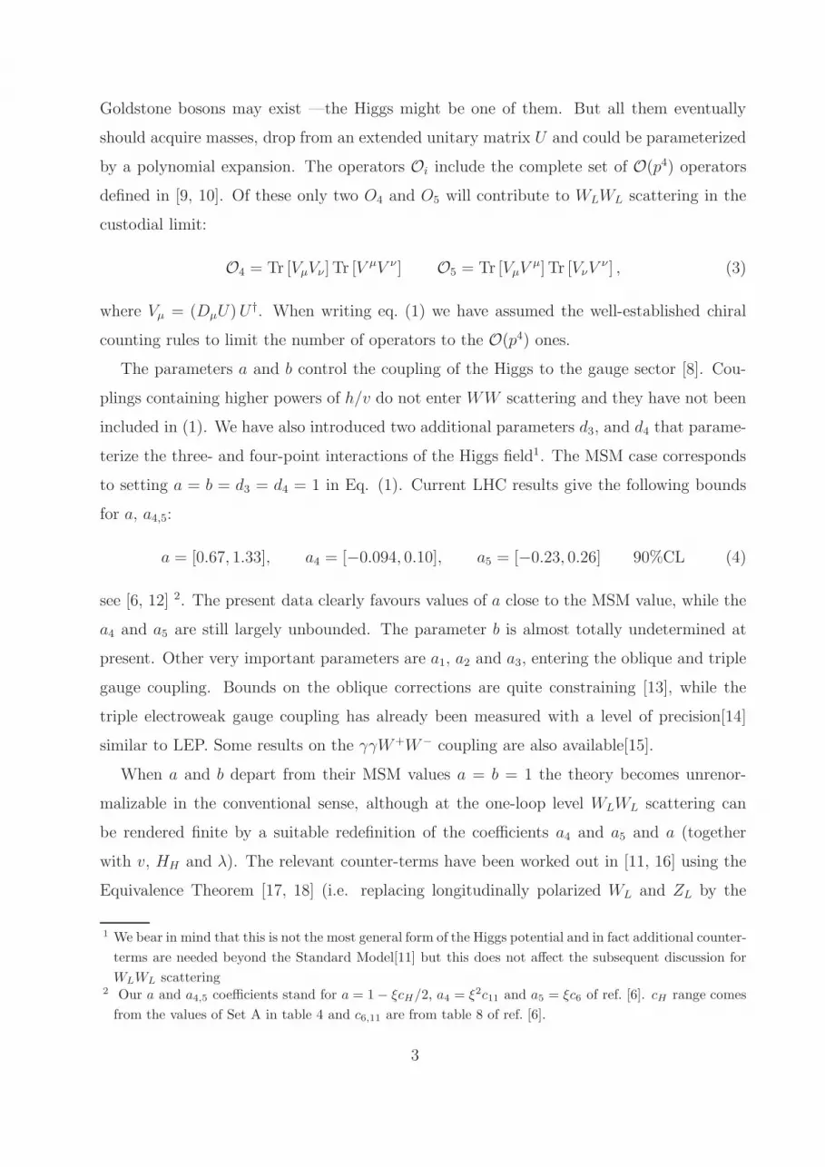
Goldstone bosons may exist —the Higgs might be one of them. But all them eventually

should acquire masses, drop from an extended unitary matrix U and could be parameterized

by a polynomial expansion. The operators Oi include the complete set of O(p4) operators

defined in [9, 10]. Of these only two O4 and O5 will contribute to WLWL scattering in the

custodial limit:

O4 = Tr [VµVν ] Tr [VµV ν ] O5 = Tr [VµV

µ] Tr [VνVν ] , (3)

where Vµ = (DµU)U †. When writing eq. (1) we have assumed the well-established chiral

counting rules to limit the number of operators to the O(p4) ones.

The parameters a and b control the coupling of the Higgs to the gauge sector [8]. Cou-

plings containing higher powers of h/v do not enter WW scattering and they have not been

included in (1). We have also introduced two additional parameters d3, and d4 that parame-

terize the three- and four-point interactions of the Higgs field1. The MSM case corresponds

to setting a = b = d3 = d4 = 1 in Eq. (1). Current LHC results give the following bounds

for a, a4,5:

a = [0.67, 1.33], a4 = [−0.094, 0.10], a5 = [−0.23, 0.26] 90%CL (4)

see [6, 12] 2. The present data clearly favours values of a close to the MSM value, while the

a4 and a5 are still largely unbounded. The parameter b is almost totally undetermined at

present. Other very important parameters are a1, a2 and a3, entering the oblique and triple

gauge coupling. Bounds on the oblique corrections are quite constraining [13], while the

triple electroweak gauge coupling has already been measured with a level of precision[14]

similar to LEP. Some results on the γγW+W− coupling are also available[15].

When a and b depart from their MSM values a = b = 1 the theory becomes unrenor-

malizable in the conventional sense, although at the one-loop level WLWL scattering can

be rendered finite by a suitable redefinition of the coefficients a4 and a5 and a (together

with v, HH and λ). The relevant counter-terms have been worked out in [11, 16] using the

Equivalence Theorem [17, 18] (i.e. replacing longitudinally polarized WL and ZL by the

1 We bear in mind that this is not the most general form of the Higgs potential and in fact additional counter-

terms are needed beyond the Standard Model[11] but this does not affect the subsequent discussion for

WLWL scattering2 Our a and a4,5 coefficients stand for a = 1− ξcH/2, a4 = ξ2c11 and a5 = ξc6 of ref. [6]. cH range comes

from the values of Set A in table 4 and c6,11 are from table 8 of ref. [6].

3

corresponding Goldstone bosons w and z). This approximation is appropriate to obtain

the relevant counter-terms for WLWL scattering and in [19] the renormalization is being

extended to the remaining ai counter-terms (i 6= 4, 5).

In this work we extend the previous analysis [10] of unitarized WLWL scattering to the

case a 6= 1 and b 6= 1, namely anomalous Higgs couplings to the gauge sector are now

considered. More specifically, we will vary a, b as well as the a4,5 parameters within the

experimental bounds of eq. (4). We use the Inverse Amplitude Method (IAM) [20] to enforce

the unitarity of longitudinally polarized WW amplitudes up to the O(p4). The calculation

of the amplitude is done avoiding the use of the Equivalence Theorem as much as possible.

The reason for this is that at the relatively low energies we are considering, the replacement

of the WL and ZL by w and z is problematic in order to make accurate predictions. In the

next sections, we will give examples of how misleading the ET can be if the right kinematical

conditions are not met.

As in the previous work [10], we found that new resonances can appear in the parameter

space of a4,5 for given values of a and b even though for values of a > 1 the allowed region

is drastically reduced by the causality constraint. More specifically, for a ≤ 1 and b free,

the overall picture is very similar to one in [10] where the case a = b = 1 (experimentally

favoured so far) was studied. In the scalar channel for example, new resonances go from

masses as low as 300 GeV to nearly as high as the cutoff of the method of 4πv ≃ 3 TeV,

with rather narrow widths typically from 10 to 100 GeV. In the vector channel the lowest

achievable masses range from about 600 GeV up to the cutoff, with widths going from 5 to

about 50 GeV. For a > 1, the picture is drastically different with respect the one in [10],

since for a large portion of the a4,5 parameter space many resonances have negative widths

breaking causality.

It is usually expected that a new strongly interacting sector would lead to resonances in

different channels but what turned out to be a bit of a surprise in our previous work [10]

and in the present for a < 1 is that these resonances are typically narrow and very hard

to detect. This appears to be directly related to the unitarization of the WLWL scattering

in the presence of light Higgs. Searching for these resonances at LHC will be however very

important because if none of them reveals itself below ∼ 3 TeV virtually all a4,5 parameter

space of the anomalous couplings could be excluded. This can be an indirect way of assessing

these quartic electroweak boson couplings. Actually, no direct information on a4 and a5

4

exists at present from direct measurements of the quartic electroweak boson couplings.

Unfortunately the actual signal strength of the new resonances predicted is such that

they are not currently being probed in LHC Higgs search data and consequently no relevant

bounds on a4 and a5 can be derived at present from the existing data —a situation that may

change soon. The previous considerations emphasize the importance of indirect measures

of the couplings a4 and a5 by searching for the additional resonances coming out from our

study of WLWL scattering. Measuring these anomalous couplings will be one of the main

tasks of the LHC run starting in 2015.

II. ISOSPIN AND PARTIAL WAVE AMPLITUDES

Here we introduce the basic definition of our observables. We shall consistently assume

our treatment that custodial symmetry is exactly preserved. This implies taking g′ = 0 and

ignoring all the Oi operators that can contribute to WW scattering but O4 and O5. This

approximation also allows for a neat usage of the isospin formalism and for the convergence

of the partial wave amplitudes. We also disregard operators that contain matter fields as

they are totally irrelevant for the present discussion.

As emphasized in [10] when dealing with longitudinally polarized amplitudes, as opposed

to using the ET approximation, caution must be exercised to account for an ambiguity

introduced by the longitudinal polarization vectors that do not transform under Lorentz

transformations as 4-vectors. Expressions involving the polarization vector ǫµL can not be

cast in terms of the Mandlestam variables s, t, and u until an explicit reference frame has

been chosen, as they can not themselves be written solely in terms of covariant quantities.

Obviously amplitudes still satisfy crossing symmetries when they remain expressed in terms

of the external 4-momenta. A short discussion on this point is placed in appendix B.

A general amplitude, A(W a(pa) + W b(pb) → W c(pc) + W d(pd)), can be written using

isospin and Bose symmetries as

Aabcd(pa, pb, pc, pd) = δabδcdA(pa, pb, pc, pd) + δacδbdA(pa,−pc,−pb, pd) (5)

+ δadδbcA(pa,−pd, pc,−pb),

5

with

A+−00 = A(pa, pb, pc, pd) (6)

A+−+− = A(pa, pb, pc, pd) + A(pa,−pc,−pb, pd)

A++++ = A(pa,−pc,−pb, pd) + A(pa,−pd, pc,−pb).

The fixed-isospin amplitudes are given by

T0(s, t, u) = 〈00|S|00〉 = 3A+−00 + A++++ (7)

T1(s, t, u) = 〈10|S|10〉 = 2A+−+− − 2A+−00 − A++++

T2(s, t, u) = 〈20|S|20〉 = A++++ .

We shall also need the amplitude for the process W+W− → hh. Taking into account that

the final state is an isospin singlet and defining

A+− = A(W+(p+) +W−(p−) → h(pc) + h(pd)) , (8)

the projection of this amplitude to the I = 0 channel gives

TH,0(s, t, u) =√3A+−. (9)

The partial wave amplitudes for fixed isospin I and total angular momentum J are

tIJ(s) =1

64π

∫ 1

−1

d(cos θ)PJ(cos θ)TI(s, t, u) , (10)

where the PJ(x) are the Legendre polynomials and t = (1 − cos θ)(4M2 − s)/2, u = (1 +

cos θ)(4M2−s)/2 with M being the W mass. We will concern ourselves with only the lowest

non-zero partial wave amplitude in each isospin channel: t00(s), t11(s), and t20(s), namely the

scalar/isoscalar, vector/isovector, and isotensor amplitudes respectively. Unitarity directly

implies that |tIJ(s)| < 1. For further implications of unitarity on tIJ(s) the interested reader

may see ref. [21].

In this work, the partial wave amplitude tIJ(s) are studied up to O(p4), namely

tIJ(s) = t(0)IJ (s) + t

(2)IJ (s) . (11)

Here t(0),(2)IJ (s) are tree-level and O(p4) contributions, respectively. t

(0)IJ (s) can be constructed

from eq. (10) by using crossing and isospin relation for the tree level contributions of A+−00

6

(Figure 1). The analytic results of A+−00 at tree-level are in appendix A. t(0)IJ (s) contains the

anomalous coupling a but b does not enter at tree-level. t(4)IJ (s) includes tree-level contribu-

tions from ai counter-terms (see appendix A for analytic result) and the one-loop corrections

to the diagrams in Figure 1. At one-loop level, the b parameters enters t(4)IJ (s) by the one-loop

expression of A+−00 calculated in ref. [16].

W+

W−

Z

Z

W+

W+

W−

Z

Z

W+

W+

W−

Z

Z

H

W+

W−

Z

Z

FIG. 1: Diagrams contributing to A(s, t, u) at tree level.

III. SCRUTINY OF THE TREE-LEVEL AMPLITUDES t(0)00 , t

(0)20 AND t

(0)11

For values of a different from 1, the WLWL scattering amplitudes exhibit rather different

behaviour with respect to the MSM case a = 1. The most important difference is that

the |tIJ | < 1 unitarity bound is violated at tree-level pretty quickly. We shall see later

how to restore unitarity with the help of higher loops and counter-terms but in this section

we concentrate on the peculiarities of the tree level amplitudes t(0)00 , t

(0)20 and t

(0)11 . Here

the partial wave amplitudes are studied in the complete theory, namely away from the ET

approximation. This is a key point since there are interesting kinematical features of t(0)IJ

that are totally missed in the ET approximation, such as the presence of sub-threshold

singularities and zeroes of t(0)IJ absent in ET approximation. Some of these features will be

crucial in our analysis.

In order to study the behaviour of t(0)IJ , we will establish three different regions according

to the range of the values of a = 1, a > 1 and a < 1.

7

A. Case a = 1

In Figure 2 we plot the tree-level isoscalar partial wave amplitude t(0)00 (s) for WLWL →

ZLZL as a function of s. The external W legs are taken on-shell (p2 = M2 = M2W = M2

Z). As

we see from Figure 2 the partial wave amplitude has a rather rich analytic structure. It has

one pole at s = M2H but also a second singularity can be seen at the value s = 3M2. A closer

examination reveals also a third singularity at s = 4M2 −M2H , invisible in the Figure 2 as

it happens to be multiplied by a very small number. These singularities correspond to poles

of the t and u channel diagrams in Figure 1 that after the angular integration of eq. (10) to

obtain the partial wave amplitudes behave as logarithmic divergences. The t and u channels

are absent in the ET approximation. Note that both singularities are below the physical

threshold at s = 4M2. Beyond the s = 3M2 singularity the amplitude for a = 1 is always

positive as can be seen in Figure 2.

In Figure 2 we also plot the tree-level partial wave amplitude t(0)11 (s). Here, a pole at

s = M2 is visible, as expected, along with the two kinematical sub-threshold singularities

already mentioned. In Figure 2 the t(0)00 and t

(0)11 amplitudes are also compared with the

respective amplitudes obtained in ET approximation. As can be seen the ET is grossly

inadequate at low energies. In particular it fails in reproducing the rich analytic structure of

the amplitudes. The non-analyticity at s = 3M2 and s = 4M2 −M2H due to sub-threshold

singularities is actually also present in the t(0)20 partial wave amplitude (not depicted), corre-

sponding like in the other two cases to a (zero width) logarithmic pole. In t(0)20 there are no

other singularities as no I = 2 particle is exchanged in the s-channel. These sub-threshold

singularities are genuine effects in the WLWL → ZZ amplitudes and are independent from

the value of a. These features are conspicuously absent in the analogous amplitude computed

in the ET.

WLWL → ZLZL scattering can be accessible at LHC by the studying the process pp →WWjj. Then, these sub-threshold singularities should be hardly visible mostly due to the

off-shellness of the WLWL → ZLZL amplitude on pp → WWjj. The experimental process

spreads the logarithmic poles over a range of invariant masses. For instance, the singularity

at s = M2 appears actually at s =∑

q2i −M2 if W legs are off-shell. In addition cuts in pT

8

ET

Exact

0 200 400 600 800 1000 1200 1400

-0.15

-0.10

-0.05

0.00

0.05

0.10

0.15

s

Re@

t 00D

Tree-Level: SM Ha=1L

ET

Exact

60 80 100 120 140 160 180 200-0.15

-0.10

-0.05

0.00

0.05

0.10

0.15

s

Re@

t 00D

Zoom HSML

H4M2-MH

2 L1�2

ET

Exact

0 200 400 600 800 1000 1200 1400

-0.15

-0.10

-0.05

0.00

0.05

0.10

0.15

s

Re@

t 11D

Tree-Level: SM Ha=1L

ET

Exact

60 80 100 120 140 160 180 200-0.15

-0.10

-0.05

0.00

0.05

0.10

0.15

s

Re@

t 11D

Zoom HSML

H4M2-MH

2 L1�2

FIG. 2: Plot of t(0)00 (above) and t11 (below) for a = 1. In both cases a zoom on the lowest values

of s to show the complete analytic structure is presented. The arrow indicates the position of one

of the sub-threshold singularities that is invisible at the scale of the plot.

should render the partial wave amplitude actually non-singular 3.

B. Case a > 1

The three sub-threshold singularities appearing at a = 1 are also present in this case.

However, for a > 1 the partial wave amplitudes also show a new features. First of all, as

shown in Figure 3 for a = 1.1 and amplitudes t(0)00 (s) and t

(0)11 (s), the tree-level partial wave

amplitude for t(0)IJ (s) show clear non-unitary behaviours as it goes to −∞ as s increases.

In addition, for a > 1 the tree-level partial wave amplitudes for t(0)IJ (s) have zeroes for

values of s above threshold and well below well below the cut-off scale (3 TeV) of our

3 We thank D. D’Enterria and X. Planells for discussions on these points.

9

effective Lagrangian. Setting for example the value a = 1.1 compatible with the experimental

constraint in eq. (4) the t(0)00 (s) amplitudes vanishes at two values of

√s around 216 and 445

GeV (see Figure 3 for a = 1.1), the t(0)11 (s) at a value around 1 TeV as well as t

(0)20 (s) at

about 800 GeV (not shown). For a > 1.125, the tree-level amplitude t(0)00 has no zeroes

(Figure 4 for a = 1.3), whereas the t(0)11 (s) and t

(0)20 (s)amplitudes for values of a compatible

with bounds in eq. (4) still vanish at specific values of√s. For example for a = 1.3, the

zeroes of t(0)11 (s) and t

(0)20 (s) are at

√s around 450 GeV. The presence of zeroes for the tree-

level amplitudes at low values of√s is interesting point as it means that around these zeroes

the WLWL → ZLZL amplitudes are strongly suppressed. It may be relevant to note that

ET

Exact

0 200 400 600 800 1000 1200 1400

-0.15

-0.10

-0.05

0.00

0.05

0.10

0.15

s

Re@

t 00D

Tree-Level: a=1.1

ET

Exact

60 80 100 120 140 160 180 200-0.15

-0.10

-0.05

0.00

0.05

0.10

0.15

s

Re@

t 00D

Zoom Ha=1.1L

H4M2-MH

2 L1�2

ET

Exact

0 200 400 600 800 1000 1200 1400

-0.15

-0.10

-0.05

0.00

0.05

0.10

0.15

s

Re@

t 11D

Tree-Level: a=1.1

ET

Exact

60 80 100 120 140 160 180 200-0.15

-0.10

-0.05

0.00

0.05

0.10

0.15

s

Re@

t 11D

Zoom Ha=1.1L

H4M2-MH

2 L1�2

FIG. 3: Plot of t(0)00 and t

(0)11 for a = 1.1 and a zoom on the low s region where the amplitude is

very small. Several additional zeroes appear above threshold and is not unitary. The ET result is

shown by (red) a dotted line.

the t(0)00 and t

(0)11 amplitudes are very small over a fairly extended range of values of s for a

range of values of a > 1 (particularly so in the isovector channel). These facts could perhaps

be used to set rather direct bounds on this particular coupling. This issue deserves further

10

phenomenological study.

ET

Exact

0 200 400 600 800 1000 1200 1400-0.3

-0.2

-0.1

0.0

0.1

0.2

0.3

s

Re@

t 00D

Tree-Level: a=1.3

ET

Exact

60 80 100 120 140 160 180 200-0.15

-0.10

-0.05

0.00

0.05

0.10

0.15

s

Re@

t 00D

Zoom Ha=1.3L

H4M2-MH

2 L1�2

ET

Exact

0 200 400 600 800 1000 1200 1400

-0.15

-0.10

-0.05

0.00

0.05

0.10

0.15

s

Re@

t 11D

Tree-Level: a=1.3

ET

Exact

60 80 100 120 140 160 180 200-0.15

-0.10

-0.05

0.00

0.05

0.10

0.15

s

Re@

t 11D

Zoom

H4M2-MH

2 L1�2

FIG. 4: Plot of t(0)00 and t

(0)11 for a = 1.3. Only the three usual singularities appear in each channel

and is non-unitary (recall that one of the singularities is not visible and their position is indicated

explicitly). There are no additional zeroes all the way up to the upper range of validity of the

effective Lagrangian. The ET results are indicated by a dotted line.

C. Case a < 1

For a < 1, the t(0)IJ amplitude still present the two sub-threshold singularities at s = 3M2

and s = 4M2 − M2H . Beyond them however, no additional zeroes appear, amplitudes are

positive and go to ∞ as s increases. This clearly reflects the non-unitary character of t(0)IJ

amplitudes for a 6= 1. In Figure 5, we show as an example the t(0)11 (s) and t

(0)20 (s) amplitudes

in the case a = 0.9. The equivalent amplitudes computed by making use of the ET are also

shown in Figure 5. Both in this a < 1 case and in the a > 1 one we see that the ET works

reasonably well for large values of s, but again fails at low and moderate values.

11

ET

Exact

0 200 400 600 800 1000 1200 1400

-0.15

-0.10

-0.05

0.00

0.05

0.10

0.15

s

Re@

t 00D

Tree-Level: a=0.9

ET

Exact

60 80 100 120 140 160 180 200-0.15

-0.10

-0.05

0.00

0.05

0.10

0.15

s

Re@

t 00D

Zoom Ha=0.9L

H4M2-MH

2 L1�2

ET

Exact

0 200 400 600 800 1000 1200 1400

-0.15

-0.10

-0.05

0.00

0.05

0.10

0.15

s

Re@

t 11D

Tree-Level: a=0.9

ET

Exact

60 80 100 120 140 160 180 200-0.15

-0.10

-0.05

0.00

0.05

0.10

0.15

s

Re@

t 11D

Zoom Ha=0.9L

H4M2-MH

2 L1�2

FIG. 5: Plots of t(0)00 and t

(0)11 for a = 0.9 and a zoom of the region at low s where the amplitudes

are very small. No additional zero appear and the amplitudes also show a non-unitary behaviour

at large s. The nearly invisible logarithmic singularity at s = 4M2 −M2H is indicated. The results

in the ET approximation are also indicated by a dotted line.

IV. UNITARITY CORRECTIONS

In the case of Higgs anomalous couplings to gauge sector (a 6= 1 and b 6= 1) the tree-level

amplitudes t(0)IJ are not-unitarity and we are forced to include additional operators in the

theory, such as the ai counter-terms in eq. (1). At one-loop level, the ai will cancel the

divergences of the Lagrangian in eq. (1) and finite couplings renormalized at some UV scale

will remain [11, 16], namely

a4|finite ≃1

(4π)2−1

12(1− a2)2 log

v2

f 2(12)

a5|finite ≃1

(4π)2−1

24

[

(1− a2)2 +3

2((1− a2)− (1− b))2

]

logv2

f 2, (13)

where f is the scale of the new interactions, and possibly other finite pieces.

12

Up to now, the calculation of the one-loop t(2)IJ (s) contribution in eq. (11) is not available

for a and b arbitrary and longitudinally polarized W and Z. This would require the evalua-

tion of over one thousand diagrams. A numerical calculation is only available in [22] for the

case a = b = 1 but it is not very useful for our purposes.

For this reason, to estimate the t(2)IJ (s) contribution in eq. (11) we proceed in the following

way. The analytic contribution from a4,5 terms are calculated exactly with longitudinally

polarized W and Z (appendix A) like the tree-level contribution t(2)IJ (s) . The real part of

t(2)IJ (s) will however be determined using the ET [17, 18]; i.e. we replace this loop amplitude

by the corresponding process w+w− → zz. For this part of the calculation we take q2 =

0 for external legs and set M = 0 but the Higgs mass is kept. The relevant diagrams

of A(ww → zz) entering t(4)IJ (s) were calculated in [16] where explicit expressions for the

different diagrams for arbitrary values of the couplings a and b can be found. This calculation

has been checked and extended in [11], albeit setting MH = 0. As to the imaginary part of

t(2)IJ (s) we can take advantage of the optical theorem to circumvent the problem of using the

ET approximation. In the I = 1, J = 1 and I = 2, J = 0 cases we can use the relations

Im t(2)IJ (s) = σ(s)|t(0)IJ (s)|2 , (14)

While for the I = 0 amplitude we also have a contribution from a two-Higgs intermediate

state. Then

Im t00(s) = σ(s)|t00(s)|2 + σH(s)|tH,0(s)|2 , (15)

with

σ(s) =

√

1− 4M2

s, σH(s) =

√

1− 4M2H

s. (16)

We believe that for the purpose of identifying dynamical resonances, normally occurring at

s ≫ M2H the approximation of relying on the ET for the real part of the loops is fine. Note

that the dominant contribution to the real part for large s, of order s2, is controlled by the

contribution coming from couplings a4,5. We have also actually checked that, unless a4 and

a5 are both very small, the contribution from the real part of the loop amounts only to a

small correction to t(2)IJ .

The final ingredient we need is a procedure to construct an unitary amplitude that per-

turbatively coincides with the tree plus one-loop result but incorporates the principle of

unitarity. To this purpose, we use the Inverse Amplitude Method (IAM) [20] to the ampli-

13

tude in eq.(11), namely

tIJ ≈ t(0)IJ

1− t(2)IJ /t

(0)IJ

, (17)

which is identical to the [1,1] Pade approximant to tIJ derived from (11). The above expres-

sion obviously reproduces the first two orders of the perturbative expansion (eq. 11)and, in

addition, satisfies the necessary unitarity constraints, namely |tIJ | < 1 at high energies and

Im tIJ(s) = σ(s)|tIJ(s)|2, (18)

when the perturbative ingredients satisfy

Im t(2)IJ (s) = σ(s)|t(0)IJ (s)|2 , (19)

as they must from the optical theorem. We refer to [10] and references therein for a more

detailed discussion. We also recommend to read the recent article [23] for a rather complete

review. In what follows we shall adhere to the procedure outlined in [10].

There is no really unambiguous way of applying the IAM to the case where there are

coupled channels with different thresholds. This will be relevant to us only in the t00 case as

there is an intermediate state consisting in two Higgs particles. Here we shall adhere to the

simplest choice that consists in assuming (17) to remain valid also in this case. In addition,

there is decoupling of the two I = 0 channels in the case a2 = b, as also discussed in [23] in

the context of the ET approximation. We have checked our results for different values of b,

in particular we see that setting b = a2 does not give for the resonances that are eventually

found results that are noticeably different from those obtained for other values of b. Finally,

we have also checked explicitly the unitarity of our results.

V. LOOKING FOR RESONANCES IN a4 AND a5 PARAMETER SPACE

Non-renormalizable models such as the effective theory described by the Lagrangian (1)

typically produce scattering amplitudes that grow too fast with the scattering energy break-

ing the unitarity bounds [21] at some point or other.

Chiral descriptions of QCD [24] are archetypal examples of this behavior and unitarization

techniques have to be used to recover unitarity. The IAM [20], described in the previous

section, is a convenient way of doing so. In QCD when the physical value of the pion decay

constant fπ and the O(p4) low energy terms Li (as defined e.g. in [24], the counterpart of

14

the ai in strong interactions) are inserted in the chiral Lagrangian and the IAM method

is used, the validity of the chiral expansion is considerably extended and one is able to

reproduce the ρ meson pole as well as many other properties of low energy QCD [20]. The

limitations of the method derive to a large extent from the accuracy in our knowledge of

the different amplitudes entering the game. Different unitarization methods (such as e.g.

N/D expansions or the Roy equations) always give very similar results as far as the first

resonances is concerned.

Any strongly interacting theory should exhibit an infinite number of resonances. This

is what hopefully one would get if all the terms in the effective expansion were included,

including all loop corrections and counter-terms. Including contributions up to O(p4), our

expression of tIJ(s) are to large extent polynomials up to order s2 (module logs). Therefore,

we can find one or two resonances—the lowest lying ones in each channel. However this

is already providing us precious information on the dynamics of the strongly interacting

theory. In the present case, the mere presence of higher resonances signals gives interesting

information on the higher order coefficients of the effective Lagrangian (1) and therefore on

WW scattering.

If instead of a new strongly interacting sector the EWSBS is perturbative, with point-

like fields (a possibility could be an extended scalar sector or two Higgs-doublet models),

integrating them out would yield no-vanishing values for the coefficients a4 and a5 [25]. The

unitarization method then reproduces approximately the masses of the particles that were

originally integrated out which is still valid information for physics beyond the SM.

To find resonances, we perform a scan for the values |a4| < 0.01 and |a5| < 0.01 and a

and b fixed looking for the presence or otherwise of resonances in the different channels. We

will consider the different cases for a 6= 1 since the case a = 1 was discussed in detail in [10].

When looking for resonances we use two different methods. First we look for a zero

of the real part of the denominator in (17) and use the optical theorem to determine the

imaginary part —i.e. the width— at that location. A second method consists in searching

directly for a pole in the complex plane. In our case both methods give very similar results,

the reason being that the widths are typically quite small. It should be stated right away

that because of the way we compute the full amplitude, with separate derivations of the

real and the imaginary parts, the analytic continuation to the whole complex plane for s

is somewhat ambiguous. Had we found large imaginary parts some doubts could be cast

15

on the results but fortunately this is not the case in virtually all of parameter space. Of

course, a mathematical zero in the denominator (i.e. a genuine pole in the amplitude tIJ) is

sometimes very difficult to get numerically, but proper resonances tend to reveal themselves

in a rather clear way nevertheless. Some difficult cases present themselves for a > 1 when

the putative resonance is close to one of the zeroes of the tree-level amplitude that appear

in this case and we had to study these situations carefully.

Physical resonances must have a positive width and are only accepted as genuine res-

onances if Γ < M/4. Theories with resonances having a negative width violate causality

and the corresponding values of the low energy constants in the effective theory are to be

rejected as leading to unphysical theories. No meaningful microscopic theory could possibly

lead to these values for the effective couplings.

A. Case a < 1

We start by considering this case where the unitarized amplitudes t(0)00 , t

(0)11 and t

(0)20 share

some properties with the ones from reference [10] for a = 1, namely the tree-level amplitude

has no zeros beyond the kinematical singularity existing at s = 3M2. In this case the sign

of the tree-level amplitude as s → ∞ is always positive in our conventions.

First of all we look for the existence of resonances. We set b = 1 and consider two

values 4 a = 0.9 and a = 0.95 compatible with experimental bound and indeed we easily

find resonances in various channels. Most of them have the right causality properties that

make the theory acceptable. However, in the I = 2, J = 0 channel we see that there is

a region in the a4 − a5 plane where causality is violated. This corresponds to the shaded

region in the lower part of Figs. 6,7 and 8 and the theories corresponding to these values

for the parameters a4, a5 are therefore not acceptable. The presence of this excluded region

is in exact correspondence with was found for the a = 1 case in [10] (and also with a similar

situation in pion physics[20]).

In Fig. 6 we show the region of parameter space in a4, a5 where isoscalar and isovector

resonances exist for the value a = 0.9 along with the isotensor exclusion region. The pattern

here has some analogies with the case a = 1 studied in [10] but proper5 resonances are

4 Other values of a have also been studied but we here present results only for these two.5 Recall that resonances are required to have, in addition to the correct causal properties, Γ < M/4.

16

-0.01

-0.005

0

0.005

0.01

-0.01 -0.005 0 0.005 0.01

a 4

a5

IAM: a =0.90, b =1.0

IsoscalarIsovectorExcluded

(a)

-0.01

-0.005

0

0.005

0.01

-0.01 -0.005 0 0.005 0.01

a 4

a5

IAM: a =0.90, b =1.0

IsoscalarExcluded

(b)

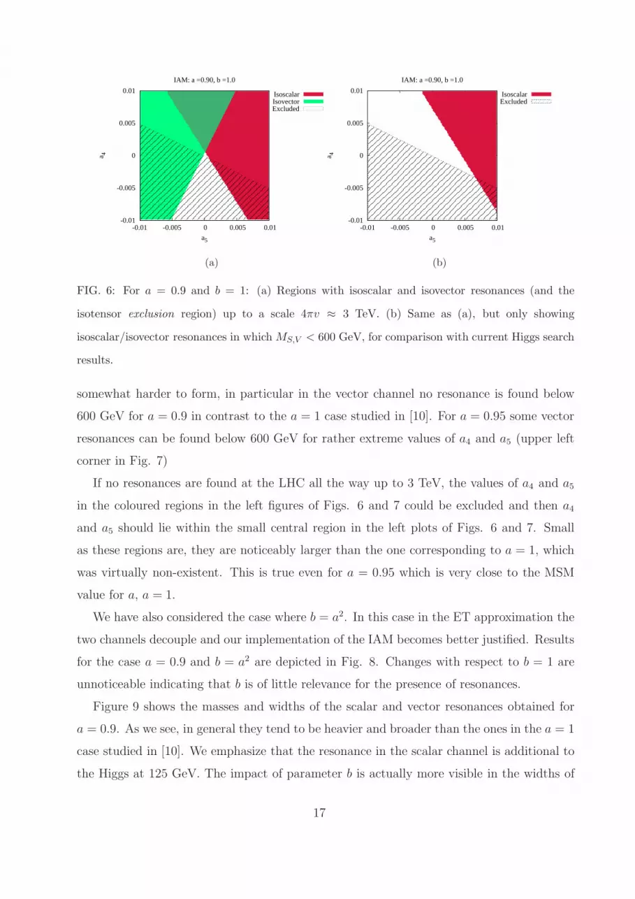
FIG. 6: For a = 0.9 and b = 1: (a) Regions with isoscalar and isovector resonances (and the

isotensor exclusion region) up to a scale 4πv ≈ 3 TeV. (b) Same as (a), but only showing

isoscalar/isovector resonances in which MS,V < 600 GeV, for comparison with current Higgs search

results.

somewhat harder to form, in particular in the vector channel no resonance is found below

600 GeV for a = 0.9 in contrast to the a = 1 case studied in [10]. For a = 0.95 some vector

resonances can be found below 600 GeV for rather extreme values of a4 and a5 (upper left

corner in Fig. 7)

If no resonances are found at the LHC all the way up to 3 TeV, the values of a4 and a5

in the coloured regions in the left figures of Figs. 6 and 7 could be excluded and then a4

and a5 should lie within the small central region in the left plots of Figs. 6 and 7. Small

as these regions are, they are noticeably larger than the one corresponding to a = 1, which

was virtually non-existent. This is true even for a = 0.95 which is very close to the MSM

value for a, a = 1.

We have also considered the case where b = a2. In this case in the ET approximation the

two channels decouple and our implementation of the IAM becomes better justified. Results

for the case a = 0.9 and b = a2 are depicted in Fig. 8. Changes with respect to b = 1 are

unnoticeable indicating that b is of little relevance for the presence of resonances.

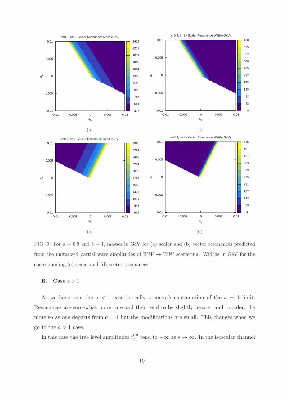
Figure 9 shows the masses and widths of the scalar and vector resonances obtained for

a = 0.9. As we see, in general they tend to be heavier and broader than the ones in the a = 1

case studied in [10]. We emphasize that the resonance in the scalar channel is additional to

the Higgs at 125 GeV. The impact of parameter b is actually more visible in the widths of

17

-0.01

-0.005

0

0.005

0.01

-0.01 -0.005 0 0.005 0.01

a 4

a5

IAM: a =0.95, b =1.0

IsoscalarIsovectorExcluded

(a)

-0.01

-0.005

0

0.005

0.01

-0.01 -0.005 0 0.005 0.01

a 4

a5

IAM: a =0.95, b =1.0

IsoscalarIsovectorExcluded

(b)

FIG. 7: For a = 0.95 and b = 1: (a) Regions with isoscalar and isovector resonances (and

the isotensor exclusion region) up to a scale 4πv ≈ 3 TeV. (b) Same as (a), but only show-

ing isoscalar/isovector resonances in which MS,V < 600 GeV, for comparison with current Higgs

search results.

-0.01

-0.005

0

0.005

0.01

-0.01 -0.005 0 0.005 0.01

a 4

a5

IAM: a =0.90, b =a2

IsoscalarIsovectorExcluded

(a)

-0.01

-0.005

0

0.005

0.01

-0.01 -0.005 0 0.005 0.01

a 4

a5

IAM: a =0.90, b =a2

IsoscalarExcluded

(b)

FIG. 8: For a = 0.9 and b = a2: (a) Regions with isoscalar and isovector resonances (and

the isotensor exclusion region) up to a scale 4πv ≈ 3 TeV. (b) Same as (a), but only showing

isoscalar/isovector resonances in which MS,V < 600 GeV. This can be compared with Fig. 6 to

conclude that b has very little relevance here.

the different resonances. In Fig. 10 we depict the widths obtained in the scalar and vector

channels for b = a2 when a = 0.9

18

a=0.9, b=1 - Scalar Resonance Mass (GeV)

-0.01 -0.005 0 0.005 0.01a5

-0.01

-0.005

0

0.005

0.01a 4

377

581

786

990

1195

1399

1604

1808

2013

2217

2422

(a)

a=0.9, b=1 - Scalar Resonance Width (GeV)

-0.01 -0.005 0 0.005 0.01a5

-0.01

-0.005

0

0.005

0.01

a 4

5

48

92

135

178

222

265

308

352

395

438

(b)

a=0.9, b=1 - Vector Resonance Mass (GeV)

-0.01 -0.005 0 0.005 0.01a5

-0.01

-0.005

0

0.005

0.01

a 4

608

843

1078

1313

1549

1784

2019

2254

2489

2724

2960

(c)

a=0.9, b=1 - Vector Resonance Width (GeV)

-0.01 -0.005 0 0.005 0.01a5

-0.01

-0.005

0

0.005

0.01

a 4

5

59

113

167

221

275

329

383

437

491

545

(d)

FIG. 9: For a = 0.9 and b = 1, masses in GeV for (a) scalar and (b) vector resonances predicted

from the unitarized partial wave amplitudes of WW → WW scattering. Widths in GeV for the

corresponding (c) scalar and (d) vector resonances.

B. Case a > 1

As we have seen the a < 1 case is really a smooth continuation of the a = 1 limit.

Resonances are somewhat more rare and they tend to be slightly heavier and broader, the

more so as one departs from a = 1 but the modifications are small. This changes when we

go to the a > 1 case.

In this case the tree level amplitudes t(0)IJ tend to −∞ as s → ∞. In the isoscalar channel

19

a=0.9, b=a2 - Scalar Resonance Width (GeV)

-0.01 -0.005 0 0.005 0.01a5

-0.01

-0.005

0

0.005

0.01a 4

6

64

121

179

237

295

352

410

468

525

583

(a)

a=0.9, b=a2 - Vector Resonance Width (GeV)

-0.01 -0.005 0 0.005 0.01a5

-0.01

-0.005

0

0.005

0.01

a 4

5

27

50

72

94

116

139

161

183

208

228

(b)

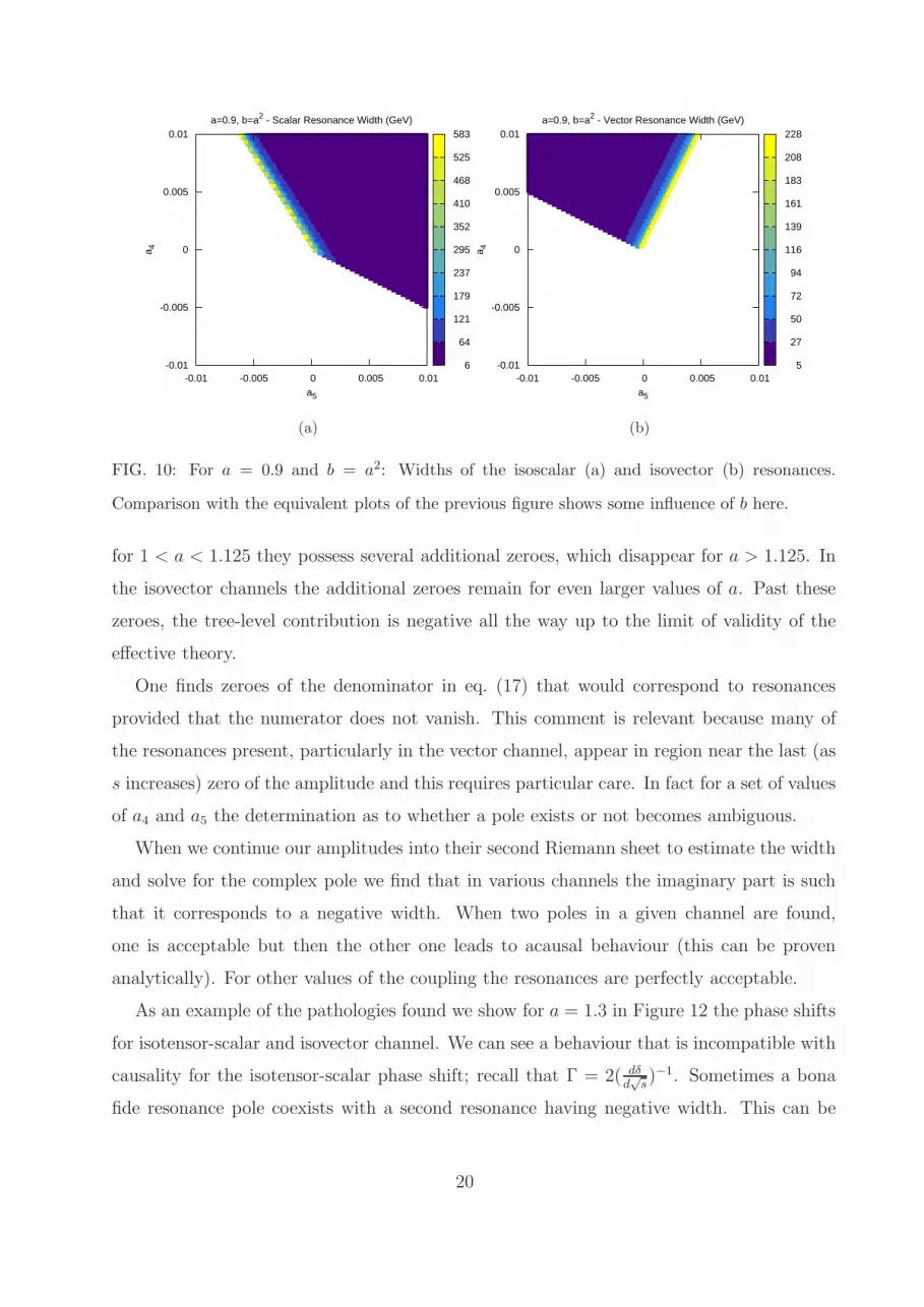
FIG. 10: For a = 0.9 and b = a2: Widths of the isoscalar (a) and isovector (b) resonances.

Comparison with the equivalent plots of the previous figure shows some influence of b here.

for 1 < a < 1.125 they possess several additional zeroes, which disappear for a > 1.125. In

the isovector channels the additional zeroes remain for even larger values of a. Past these

zeroes, the tree-level contribution is negative all the way up to the limit of validity of the

effective theory.

One finds zeroes of the denominator in eq. (17) that would correspond to resonances

provided that the numerator does not vanish. This comment is relevant because many of

the resonances present, particularly in the vector channel, appear in region near the last (as

s increases) zero of the amplitude and this requires particular care. In fact for a set of values

of a4 and a5 the determination as to whether a pole exists or not becomes ambiguous.

When we continue our amplitudes into their second Riemann sheet to estimate the width

and solve for the complex pole we find that in various channels the imaginary part is such

that it corresponds to a negative width. When two poles in a given channel are found,

one is acceptable but then the other one leads to acausal behaviour (this can be proven

analytically). For other values of the coupling the resonances are perfectly acceptable.

As an example of the pathologies found we show for a = 1.3 in Figure 12 the phase shifts

for isotensor-scalar and isovector channel. We can see a behaviour that is incompatible with

causality for the isotensor-scalar phase shift; recall that Γ = 2( dδd√s)−1. Sometimes a bona

fide resonance pole coexists with a second resonance having negative width. This can be

20

(a) (b)

FIG. 11: (a) The two resonances that appear in the scalar channel are shown in a 3D plot. The

larger one has a large negative width. The corresponding contour plot in shown in (b) where the

physical one is nearly invisible being extremely narrow.

seen for instance in Fig. 11 in the scalar channel for a = 1.1. We see that one genuine looking

resonance coexists with a huge singularity having a large negative width. The corresponding

effective theory is unacceptable.

The net result is that a very sizeable part of the space of parameters is ruled out. For

instance in Fig. 13 we show the excluded areas for a = 1.1, Fig. 13(a) and a = 1.3, Fig. 13(b).

We have seen that pathologies abound in the a > 1 case. In particular we have been

unable to find a bona fide I = 2 resonance for a = 1.1 and a = 1.3 and this seems to be the

generic situation for a > 1. This result is at odds with a recent dispersion relation analysis

[26] claiming that theories having a > 1 must show a dominance of the I = 2 channel and

even a model with a I = 2 resonance is suggested. An explanation for the discrepancy is

given in appendix D.

VI. EXPERIMENTAL VISIBILITY OF THE RESONANCES

One thing is having a resonance and a very different one is being able to detect it. In

particular the statistics so far available from the LHC experiments is limited. Searching

for new particles in the LHC environment is extremely challenging. Yet a particle with the

properties of the Higgs has been found with only limited statistics. This has been possible

21

500 600 700 800 900 1000

-Π

2

-Π

4

0

Π

4

Π

2

s

∆00HsL

a=1.3, b=1: a4= 0.001 & a5=-0.001

(a)

379.0 379.2 379.4 379.6 379.8 380.0-Π

2

-Π

4

0

Π

4

Π

2

s

∆11HsL

a=1.3, b=1: a4= 0.001 & a5=-0.001

(b)

500 550 600 650 700 750 800

-Π

2

-Π

4

0

Π

4

Π

2

s

∆20HsL

a=1.3, b=1: a4= 0.001 & a5=-0.001

(c)

FIG. 12: Phase shifts for a4 = 0.001 and a5 = −0.001 and the values a = 1.3 and b = 1. The

plots shows wrong resonances for isoscalar (≃ 760 GeV) and tensor (≃ 570 GeV) since the shift

is from −π/2, whereas isovector has a good resoances (≃ 380 GeV). Moreover, the second tensor

resonances (≃ 665 GeV) with positive width is also shown.

in part because of a fortunate upwards statistical fluctuation but also because the couplings

and other properties of the Higgs were well known in the MSM. This is not necessarily the

case for new resonances they may exist in the EWSBS. Fortunately the IAM method is

able not only of predicting masses and widths but also their couplings to the WLWL and

ZLZL channels. In [10], where the case a = 1 was considered, the experimental signal of the

different resonances was compared to that of a MSM Higgs with an identical mass. Because

the decay modes are similar (in the vector boson channels that is) and limits on different

Higgs masses are well studied this is a practical way of presenting the results.

Therefore in order to gain some intuition as to whether any of the predicted resonances

22

(a) (b)

FIG. 13: (a) Search for resonances for a = 1.1 up to the scale 4πv ≈ 3 TeV. The lower part of

parameter space is excluded due to the isotensor resonance becoming acausal. In addition there

is an exclusion area due to unphysical poles in the I = 0 channel. Some isovector and isoscalar

resonances are possible. In the white area in the upper left corner the scalar resonances are very

broad and are not considered as such by the Γ < M/4 condition. (b) Same as (a) for a = 1.3. The

areas excluded due to resonances developing negative widths are now even larger. No resonance

satisfying our criteria exists in the scalar channel, the apparent poles have all negative widths for

I = 0. In a sizeable area vector resonances develop a second unphysical resonance. As for the

isotensor channel, most of the parameter space has one pole with negative width. Then a second

exclusion band (similar to the isovector one for a = 1.1) exist due to isotensor channels having one

valid resonance together with a second acausal one. Only a small set of values present one valid

resonance in the isovector channel. Note that a4 = a5 = 0 is unphysical for a = 1.3.

for a < 1 should have been seen by now at the LHC we compare their signal (the size

of the corresponding Breit-Wigner resonance) with the one of the Higgs at an equivalent

mass. Just to gain some intuition on this we have used the easy-to-implement Effective

W Approximation, or EWA [27]. The results are depicted in Fig. 14 for the WLWL and

ZLZL vector fusion channels. Note that both production modes are sub-dominant at the

LHC with respect to gluon production mediated by a top-quark loop and also note that the

decay modes of the resonances can be predicted with the technology presented here only for

WLWL and ZLZL final states.

What can be seen in these figures is that the signal is always lower than the one for

a Higgs boson of an equivalent mass. However, the ratio σresonance/σHiggs seems to depend

substantially on the value of a. For instance, for a = 1 it was found that in the scalar channel

23

a=0.9, b=1 - WW Scalar Resonance Fraction σ/σSM

-0.01 -0.005 0 0.005 0.01a5

-0.01

-0.005

0

0.005

0.01

a 4

0.002

0.051

0.100

0.149

0.198

0.247

0.296

0.345

0.394

0.443

0.492

(a)

a=0.9, b=1 - WW Vector Resonance Fraction σ/σSM

-0.01 -0.005 0 0.005 0.01a5

-0.01

-0.005

0

0.005

0.01

a 4

0.0004

0.0389

0.0774

0.1160

0.1545

0.1930

0.2315

0.2700

0.3086

0.3471

0.3856

(b)

a=0.9, b=1 - ZZ Scalar Resonance Fraction σ/σSM

-0.01 -0.005 0 0.005 0.01a5

-0.01

-0.005

0

0.005

0.01

a 4

0.100

0.126

0.152

0.178

0.203

0.229

0.255

0.281

0.307

0.333

0.359

(c)

FIG. 14: For a = 0.9 and b = 1: Ratios of WLWL scattering cross section due to dynamical

resonances with that of the SM with a Higgs boson of the same mass for (a) scalar and (b) vector

resonances, taken in the peak region as defined in [10]. Ratio of the ZLZL scattering cross section

due to dynamical resonances with that of the SM with a Higgs boson of the same mass for a

scalar resonance (c). The LHC energy has been taken to be 8 TeV and the EWA approximation is

assumed.

this ratio was typically lower than 0.1 and only in some very limited sector of parameter

space could be as large as 0.3. It was even lower for ZZ production. Now for a = 0.9 we

see that 0.2 is a more typical value for σresonance/σHiggs and in some areas of parameter space

can go up to ∼ 0.4 or even close to 0.5. Again the signal is somewhat lower in the ZLZL

production channel. For the vector channel and again normalizing to the Higgs signal we

get ratios for σresonance/σHiggs the signal ranges from 0.03 to 0.3.

24

VII. CONCLUSIONS

In this paper we have extended the analysis of [10] to the case a 6= 1 and b 6= 1 imposing

the require of unitarity on the fixed isospin amplitudes contributing to longitudinal W

scattering. The method chosen to unitarize the partial waves is the Inverse Amplitude

Method. The simplicity of this method makes it suitable to analyze the problem being

considered, while its validity has been well tested in strong interactions in the past.

We have seen that even in the presence of a light Higgs, it can help constrain anomalous

couplings by helping predict heavier resonances, present in an extended EWSBS. The results

for a 6= 1 presented here turn out to be partly in line with the results for a = 1 previously

obtained if a < 1 and partly qualitatively different if a > 1 . If a < 1 for a large subset of

values of the higher dimensional coefficients resonances are present. Typically they tend to

be heavier and broader than in the a = 1 case. but only moderately so. They are never

like the broad resonances that were entertained in the past in Higgsless models and this is

undoubtedly a consequence of the unitarization that the presence of the Higgs brings about.

There is a smaller room for new states once unitarity is required. The properties of the

resonance are therefore radically different from the initial expectations concerning WLWL

scattering

Current LHC Higgs search results do not yet probe the IAM resonances, but it may be

possible in the near future, this is particularly true if a departs from its Standard Model

value a = 1 because the resonances become higher and broader in this case with values

for the ratio to the experimental signal that a Higgs with an equivalent mass would give

σresonance/σHiggs can get close to 0.5 (recall that this applies only to the longitudinal vector

gauge boson fusion channel). In any case it seems that LHC@14 TeV will be able to probe

a reasonable part of the possible parameter space for resonances.

If resonances are found with the properties predicted here this discovery would immedi-

ately indicate that there is an extended EWSBS and that this is likely described by some

strongly interacting theory, giving credit to the hypothesis of the Higgs being a composite

state —most likely a pseudo-Goldstone boson. It would also provide immediate information

on the value of some of the higher dimensional coefficients in the effective theory, probably

much earlier that direct WLWL scattering would allow for a determination of the quartic

gauge boson coupling.

25

We have also found another interesting result, namely that in the present framework

theories with a > 1 are nearly excluded as the IAM predicts that they lead to resonances

that violate causality in a large part of parameter space, the more so as one departs more

from a = 1..

Acknowledgements

We thank A. Dobado, J. Gonzalez-Fraile, M.J. Herrero, J.R. Pelaez, B. Yencho for discus-

sions concerning different aspects of unitarization and effective lagrangians. We acknowledge

the financial support from projects FPA2010-20807, 2009SGR502 and CPAN (Consolider

CSD2007-00042).

[1] G. Aad et al. [The ATLAS collaboration], Phys. Lett. B 716 (2012) 1.

[2] S. Chatrchyan et al. [The CMS collaboration], Phys. Lett. B 716 (2012) 30.

[3] M. Redi and A. Tesi, JHEP 1210 (2012) 166; G. Panico, M. Redi, A. Tesi and A. Wulzer,

JHEP 1303 (2013) 051

[4] D. Buttazzo, G. Degrassi, P. P. Giardino, G. F. Giudice, F. Sala, A. Salvio and A. Strumia,

JHEP 1312 (2013) 089.

[5] A. Pomarol and F. Riva, JHEP 1401, 151 (2014) [arXiv:1308.2803 [hep-ph]]; M. Montull,

F. Riva, E. Salvioni and R. Torre, Phys. Rev. D 88, 095006 (2013) [arXiv:1308.0559 [hep-ph]];

P. P. Giardino, K. Kannike, I. Masina, M. Raidal and A. Strumia, arXiv:1303.3570 [hep-ph];

T. Alanne, S. Di Chiara and K. Tuominen, JHEP 1401, 041 (2014) [arXiv:1303.3615 [hep-ph]].

[6] I. Brivio, T. Corbett, O. J. P. Eboli, M. B. Gavela, J. Gonzalez-Fraile, M. C. Gonzalez-Garcia,

L. Merlo and S. Rigolin, JHEP 1403, 024 (2014) [arXiv:1311.1823 [hep-ph]].

[7] J. Elias-Miro, J. R. Espinosa, E. Masso and A. Pomarol, JHEP 1311, 066 (2013)

[arXiv:1308.1879 [hep-ph]]; JHEP 1308, 033 (2013) [arXiv:1302.5661 [hep-ph]]; E. E. Jenk-

ins, A. V. Manohar and M. Trott, JHEP 1310, 087 (2013) [arXiv:1308.2627 [hep-ph]]; JHEP

1310, 087 (2013) [arXiv:1308.2627 [hep-ph]]; G. Buchalla, O. Cat and C. Krause, Nucl. Phys.

B 880, 552 (2014) [arXiv:1307.5017 [hep-ph]].

[8] G. F. Giudice, C. Grojean, A. Pomarol and R. Rattazzi, JHEP 0706, 045 (2007)

26

[hep-ph/0703164]; R. Contino, M. Ghezzi, C. Grojean, M. Muhlleitner and M. Spira,

arXiv:1303.3876 [hep-ph]; R. Alonso, M. B. Gavela, L. Merlo, S. Rigolin and J. Yepes, Phys.

Lett. B 722, 330 (2013) [arXiv:1212.3305 [hep-ph]].

[9] A. Dobado, D. Espriu and M.J. Herrero, Phys.Lett. B255 (1991) 405; D. Espriu and M.J.

Herrero, Nucl.Phys. B373 (1992) 117; M.J. Herrero and E. Ruiz-Morales, Nucl.Phys. B418

(1994) 431; Nucl. Phys. B 437 (1995) 319; D. Espriu and J. Matias, Phys.Lett. B341 (1995)

332; A. Dobado, M.J. Herrero, J.R. Pelaez and E. Ruiz-Morales, Phys. Rev. D 62 (2000) 05501;

R. Foadi, M. Jarvinen and F. Sannino, Phys. Rev. D 79, 035010 (2009) [arXiv:0811.3719 [hep-

ph]].

[10] D. Espriu and B. Yencho, Phys. Rev. D 87, no. 5, 055017 (2013).

[11] R. Delgado, A. Dobado and F. Llanes, arXiv:1311.5993.

[12] A. Falkowski, F. Riva and A.Urbano, JHEP 1311, 111 (2013);

[13] A. Pich, I. Rosell, J.J. Sanz-Cillero, Phys.Rev.Lett. 110 (2013) 181801; A. Pich, I. Rosell and

J.J. Sanz-Cillero, JHEP 1401 (2014) 157.

[14] S. Chatrchyan et al. [The CMS collaboration], CMS-PAS-SMP-13-005; G. Aad et al. [The

ATLAS collaboration], ATLAS-CONF-2013-020.

[15] S. Chatrchyan et al. [The CMS collaboration], JHEP 1307, 116 (2013).

[16] D. Espriu, F. Mescia and B. Yencho, Phys. Rev. D 88, 055002 (2013).

[17] J.M. Cornwall, D.N. Levin and G.Tiktopoulos, Phys. Rev. D10 (1974) 1145; C. E. Vayonakis,

Lett. Nuovo Cim. 17, 383 (1976).; B.W. Lee, C. Quigg and H. B. Thacker, Phys. Rev. D16

(1977) 1519; G.J. Gounaris, R. Kogerler and H. Neufeld, Phys. Rev. D34 (1986) 3257; M.S.

Chanowitz and M.K. Gaillard, Nucl. Phys. B261 (1985) 379; A. Dobado and J.R. Pelaez,

Nucl.Phys. B425 (1994) 110; Phys. Lett. B329 (1994) 469; C. Grosse-Knetter and I.Kuss,

Z.Phys. C66 (1995) 95; H.J.He,Y.P.Kuang and X.Li, Phys. Lett. B329 (1994) 278.

[18] D. Espriu and J. Matias, Phys. Rev. D 52 (1995) 6530.

[19] R. Delgado, A. Dobado and M.J. Herrero, in preparation (private communication, 2014)

[20] T.N. Truong, Phys. Rev. Lett. 61 (1988) 2526; A. Dobado, M.J. Herrero and T.N. Truong,

Phys.Lett. B235 (1990) 134; A. Dobado and J.R. Pelaez, Phys. Rev. D 47 (1993) 4883; Phys.

Rev. D 56 (1997) 3057; J.A. Oller, E. Oset and J.R. Pelaez, Phys. Rev. Lett. 80 (1998) 3452;

Phys. Rev. D 59 (1999) 0740001; 60 (1999) 099906(E); F. Guerrero and J.A. Oller, Nucl. Phys.

B 537 (1999) 459; A. Dobado and J.R. Pelaez, Phys. Rev D 65 (2002) 077502.

27

[21] A.D. Martin and T.D. Spearman, Elementary Particle Theory, North Holland (1970).

[22] A. Denner, S. Dittmaier, T. Hahn, Phys.Rev. D56 (1997) 117; A. Denner and T. Hahn,

Nucl.Phys. B525 (1998) 27.

[23] R. Delgado, A. Dobado and F. Llanes, J.Phys. G 41,025002 (2014).

[24] J. Gasser and H. Leutwyler, Annals Phys. 158 (1984) 142; Nucl.Phys. B250 (1985) 465;

Nucl.Phys. B250 (1985) 517.

[25] D. Espriu and P. Ciafaloni, Phys. Rev. D. 56, 1752 (1997).

[26] A. Falkowski, S. Rychkov and A. Urbano, JHEP 1204 (2012) 073; A. Urbano, arXiv:1310.5733

[hep-ph].

[27] G. L. Kane, W. W. Repko and W. B. Rolnick, Phys. Lett. B 148, 367 (1984); S. Dawson,

Phys. B 249, 42 (1985); M. S. Chanowitz and M. K. Gaillard, Nucl. Phys. B 261, 379 (1985).

Appendix A: Tree-level WLWL scattering amplitudes

In the isospin limit, M = MZ = MW , and with massive W , the tree-level and a4,5-dependent

amplitude for W+L W−

L → ZLZL scattering is given by

Atree+aiW+W−→ZZ

(p1, p2, p3, p4) = −2g2(1− g2a5)(ǫ1 · ǫ2)(ǫ3 · ǫ4) (A1)

+g2(1 + g2a4)[

(ǫ1 · ǫ4)(ǫ2 · ǫ3) + (ǫ1 · ǫ3)(ǫ2 · ǫ4)]

+g2

{

(

1

(p1 − p3)2 −M2

)

[

−4(

(ǫ1 · ǫ2)(p1 · ǫ3)(p2 · ǫ4) + (ǫ1 · ǫ4)(p1 · ǫ3)(p4 · ǫ2) +

(ǫ2 · ǫ3)(p3 · ǫ1)(p2 · ǫ4) + (ǫ3 · ǫ4)(p3 · ǫ1)(p4 · ǫ2))

+2(

(ǫ2 · ǫ4)(

(p1 · ǫ3)(p2 + p4) · ǫ1 + (p3 · ǫ1)(p2 + p4) · ǫ3)

+

(ǫ1 · ǫ3)(

(p2 · ǫ4)(p1 + p3) · ǫ2 + (p4 · ǫ2)(p1 + p3) · ǫ4))

−(ǫ1 · ǫ3)(ǫ2 · ǫ4)(

(p1 + p3) · p2 + (p2 + p4) · p1)

]

+ (p3 ↔ p4)

}

− g2M2

(

(ǫ1 · ǫ2)(ǫ3 · ǫ4)(p1 + p2)2 −M2

H

)

,

where ǫi = ǫL(pi). The analogous expression in the ET approximation is much simpler

Atree+ aiw+w−→zz

(s) = −( s

v2

)

(

(a2 − 1)s+M2H

s−M2H

− 2( s

v2

)

(

a4(1 + cos2 θ) + 4a5)

)

(A2)

28

For completeness, we also give the amplitude for the W+L W−

L → hh scattering

AtreeW+W−→hh(p1, p1, q3, q4) = g2

(

b

2(ǫ1 · ǫ2)−

3aM2H

2(M2H − (p1 + p2)2)

(ǫ1 · ǫ2) (A3)

+a2g2v2

4M2

(

(ǫ1 · (q3 − p1))(ǫ2 · (q3 − p1))−M2(ǫ1 · ǫ2)M2 − (q3 − p1)2

+ (q3 ↔ q4)

))

,

In the CM reference frame the expression for Atree+aiW+W−→ZZ

(s, t, u) becomes

Atree+ aiW+W−→ZZ

(s, t, u) =a2 (s− 2M2)

2

v2 (M2H − s)

(A4)

+768M10 − 128M8(5s+ 4t) + 32M6 (7s2 + 8st+ 4t2)

v2 (s− 4M2)2 (M2 − t) (−3M2 + s+ t)

− 8M4s (5s2 + 11st+ 4t2) +M2s2 (3s2 + 18st+ 14t2)− s3t(s+ t)

v2 (s− 4M2)2 (M2 − t) (−3M2 + s+ t)

+8a5(s− 2M2)2 + 2a4(16M

4 − 8M2s+ (1 + cos2 θ)s2))

v4

Recall that Atree+ aiW+W−→ZZ

(s, t, u) for the scattering of longitudinally polarizedW is not Lorentz

invariant. The expression above is valid in CM frame only.

Appendix B: The issue of crossing symmetry

We would like to clarify the issue of crossing symmetry of amplitudes with external WL’s.

To this end let us consider just the tree-level contribution in the MSM to the processes

W+L W−

L → W+L W−

L and W+L W+

L → W+L W+

L , respectively.

To keep the formulae simple while making the point let us consider the limit s → ∞,

−t → ∞ in the first process, which is consistent except for cos θ ≃ 1, and expand in M2/s

and M2/t. We borrow the results from [18]. The resulting amplitude is

− g2(

M2H

4M2

[

t

t−M2H

+s

s−M2H

]

+s2 + t2 + st

2st− M2

H

s

2M2Ht− s(s+ t)

(M2H − s)(M2

H − t)

)

+ . . . . (B1)

In the second process we expand in powers of M2/u and M2/t. One then gets

−g2(

M2H

4M2

[

t

t−M2H

+u

u−M2H

]

+u2 + t2 + ut

2ut+

M2H

t + u

(t− u)2

(M2H − u)(M2

H − t)

)

+ . . . . (B2)

The two processes are related by crossing and one would naively think that the two am-

plitudes can be related by simply exchanging s and u. While this is correct for the first

two terms in both equations, it fails for the third. If the reader is worried about the ap-

proximations made, more lengthy complete results are given in [18] and they show the same

features.

29

The reason is that while crossing certainly holds when exchanging the external four

vectors, the reference frame in which the two above amplitudes are expressed are different. In

both cases they correspond to center-of-mass amplitudes, but after the exchange of momenta

the two systems are boosted one with respect to the other. Writing the amplitudes in terms

of s, t, u gives the false impresion that these expressions hold in any reference system but

this is not correct because the polarization vectors are no true four-vectors.

On the contrary, the amplitudes computed via the ET are manifestly crossing symmetric

because they amount to replacing ǫµL → kµ, which is obviously a covariant 4-vector. We

insist once more that crossing does hold in any case but is not manifest for the scattering of

longitudinal W bosons at the level of Mandelstam variables.

Appendix C: The origin of the logarithmic poles

Here we discuss the origins of the 3 singularities at s0 = M2H , s1 = 4M2 − M2

H and

s2 = 3M2) entering the tIJ(s) amplitudes. These singularities can be tracked back from the

terms 1/(s−M2H), 1/(t−M2) and 1/(u−M2) in the W+

L W−L → ZLZL amplitude in eq. A4.

The origin of the pole at s0 is fairly obvious and needs no justification.

As for the other two singularities, the term 1/(t − M2) = 1/((−1 + cos θ)(−4M2 +

s)/2 − M2) has a pole at s3 for cos θ = −1 which under integration in cos θ to derive

the partial wave amplitude tIJ(s) becomes a logarithmic pole as well as for 1/(u −M2) =

1/((1 + cos θ)(−4M2 + s)/2−M2) at cos θ = −1. This explains the presence of s2 pole for

tIJ(s) amplitudes.

The origin of the pole at s1 for tIJ(s) amplitudes is more complicated to see. First of all,

let us notice that the fixed-isospin amplitudes TI in eq. 7 are combinations of the A++00 =

A(W+L W−

L → ZLZL) in eq. A4 and its crossed amplitude A++++ = A(W+L W+

L → W+L W+

L ).

At this point, the term 1/(s −M2H) in A++00, eq. A4, trasforms for the crossed amplitude

A++++ into 1/(t −M2H) = (1/(−1 + cos θ)(−4M2 + s)/2 −M2

H). Then, for cos θ = −1 we

have a pole at s1 and under integration on cos θ the amplitude tIJ(s) gets a logarithmic pole

at s1.

Note that these singularities are all below threshold. Note too that except for s0 they are

absent in the ET treatment. For the LHC they appear at values of s corresponding to the

replacement 4M2 →∑

i q2i as the external W are typically off-shell.

30

Appendix D: Sum rule

In [26] the following sum rule was derived

1− a2

v2=

1

6π

∫ ∞

0

ds

s

(

2σI=0(s)tot + 3σI=1(s)

tot − 5σI=2(s)tot)

, (D1)

where σtotI is the total cross section in the isospin channel I. This interesting result was

derived making full use of the Equivalence Theorem and setting M = 0. As we have seen, at

low s there are some relevant deviations with respect to the ET predictions when using the

proper longitudinal vector boson amplitudes and they affect the analytic properties of the

amplitude. We would like to see how this sum rule could be affected by these deviations.

The technique used in [26] to derive the previous result was to define the function

F (s, t, u) = AtreeW+W−→ZZ(s, t, u)/s

2, consider the case t = 0, corrresponding to the forward

amplitude, and compute the integral

∮

dsF (s, t, u) (D2)

using two different circuits: one around the origin and another one along the cuts in the

real axis and closing at infinity (this last contribution actually drops if the amplitudes are

assumed to grow slower than s).

Applying the strict ET, each order in perturbation theory contributes to a given order in

an expansion in powers of s, t, u. Therefore if the integral is done in a small circle around

the origin only the tree-level amplitude eq. (A2) contributes and taking both contributions

into account results in the result on the left hand side of equ. (D1). On the other hand, the

integral along the left cut can be related using crossing symmetry to the one on the right

cut and eventually leads to the right hand side of equation (D1).

Formulae (A1) and (A2) show clearly that the analytic structure of the full result and

the ET one are quite different at low values of s. In the exact case and for the tree-level

amplitude we have four poles for F (s, t, u). We assume that s and t are independent variables

31

and to make this visible we replace t → t

s0 = 0 → Res(F (s0, t, u)) =4a2M2(M2 −M2

H)

M4Hv

2+

2t (8M4 − 7M2t+ t2)

v2 (M2 − t) (t− 3M2)2

s1 = M2H → Res(F (s1, t, u)) = −a2 (M2

H − 2M2)2

M4Hv

2

s2 = 3M2 − t → Res(F (s2, t, u)) = −−27M8 + 52M6t +M4t2 + 2M2t3

v2 (t− 3M2)2 (M2 + t)2

s3 = 4M2 → Res(F (s3, t, u)) = t10M4 − 3M2t− 3t2

(M2 − t)(M2 + t)2v2(D3)

∑

i=0,3

Res(F (si, t, u)) =(3− a2)M2 − (1− a2)t

(M2 − t)v2(D4)

Note however that for s = s3 = 4M2, the t variable is always zero, being t = −(1 −cos θ)(s−4M2)/2, and u = −(1+cos θ)(s−4M2)/2. This shows that s and t are dependent

for some exceptional kinematical points, for example when the inicial states are at rest

(s = s3 = 4M2). Therefore when s → s3, t → 0. If we set t = 0 at the outset the sum of

residues leads to∑

i=0,3

Res(F (si, t = 0, u)) =(3− a2)

v2. (D5)

which differs from the result quoted in [26]. The reason is clear when looking at eq. (D4):

if we take the limit M → 0 at the outset as is done in the strict ET approximation, we get

one result, while if t is set to zero with M 6= 0, we get a different one.

In addition, in a complete calculation (as opposed to the simpler ET treatment) it is

not true that a given order in the chiral expansion corresponds to a definite power of s.

Therefore, when M is not neglected the order s contribution will have corrections from all

orders in perturbation theory. The contribution to the left hand side of the integral, obtained

after circumnavigating all the poles will then be of the form

3− a2 +O(g2)

v2. (D6)

Actually, the right cut changes too when M is taken to be non-zero; it starts at s = 4M2

(which is not a pole as we have just discussed because it has a vanishing residue). The left

cut is not changed as for t = 0 the u channel has a cut for s < 0 corresponding to u > 4M2.

Finally, as we have seen, crossing symmetry is not manifest (see appendix B) for the full

amplitudes and it is not possible to relate exactly the contribution along the left cut to the

analogous integral along the right one.

32