Unclassified STD/DOC(2012)5 Organisation de Coopération et de Développement Économiques Organisation for Economic Co-operation and Development 16-Jan-2013 ___________________________________________________________________________________________

English - Or. English STATISTICS DIRECTORATE

OECD COMPOSITE LEADING INDICATORS FOR G7 COUNTRIES: A COMPARISON OF THE HODRICK-PRESCOTT FILTER AND THE MULTIVARIATE DIRECT FILTER APPROACH STATISTICS DIRECTORATE

WORKING PAPER No 49

This paper has been prepared by Gyorgy Gyomai (OECD/STD) and Marc Wildi (IDP, Zurich University of Applied Sciences)

For further information please contact: Gyorgy Gyomai: gyorgy.gyomai@oecd.org Marc Wildi: Marc.Wildi@zhaw.ch

JT03333359

Complete document available on OLIS in its original format This document and any map included herein are without prejudice to the status of or sovereignty over any territory, to the delimitation of international frontiers and boundaries and to the name of any territory, city or area.

STD/D

OC

(2012)5 U

nclassified

English - O

r. English

STD/DOC(2012)5

OECD STATISTICS WORKING PAPER SERIES

The OECD Statistics Working Paper Series - managed by the OECD Statistics Directorate – is designed to make available in a timely fashion and to a wider readership selected studies prepared by OECD staff or by outside consultants working on OECD projects. The papers included are of a technical, methodological or statistical policy nature and relate to statistical work relevant to the Organisation.

The Working Papers are generally available only in their original language - English or French - with a summary in the other. Comments on the papers are welcome and should be communicated to the authors or to the OECD Statistics Directorate, 2 rue André Pascal, 75775 Paris Cedex 16, France.

The opinions expressed in these papers are the sole responsibility of the authors and do not necessarily reflect those of the OECD or of the governments of its Member countries.

This document and any map included herein are without prejudice to the status of or sovereignty over any territory, to the delimitation of international frontiers and boundaries and to the name of any territory, city or area.

________________________________________________________

www.oecd.org/std/publicationsdocuments/workingpapers/

________________________________________________________

© OECD/OCDE, 2012 Applications for permission to reproduce or translate all or part of this material should be made to: OECD Publications, 2 rue André-Pascal, 75775 Paris, Cedex 16, France; e-mail: rights@oecd.org

STD/DOC(2012)5

3

ABSTRACT

We estimate the business-cycles of G7 countries, as defined by an ideal 2-10 year bandpass filter applied to country-specific GDP target series (GDP-BP). Since this target series cannot be observed in real-time, due to the symmetry of the bandpass filter, we analyze and compare the leading performances of the well-known HP-filter, as currently implemented in the OECD CLI’s, as well as of the Multivariate Direct Filter Approach (MDFA) relying on explanatory time series, as selected for current CLIs. The paper shows that efficiency gains by MDFA over HP are substantial along the full revision-sequence and they are consistent across countries as well as over time, when referenced against GDP-BP.

RÉSUMÉ

Nous estimons les cycles économiques des pays du G7, définis par un filtre passe-bande idéal de 2 - 10 ans appliqué à des séries du PIB spécifiques à chaque pays. Comme cette série cible ne peut être observée en temps réel, en raison de la symétrie du filtre passe-bande, nous analysons et comparons les caractéristiques avancées du filtre HP bien connu, tel qu'il est actuellement implémenté pour le calcul des indicateurs composites avancés de l’OCDE, ainsi que l’approche par le filtre direct multivarié (MDFA), en s’appuyant sur les séries temporelles actuellement utilisées pour les indicateurs composites avancés. Ce document montre que des gains d'efficacité du filtre direct multivarié par rapport au filtre HP sont considérables au cours de la séquence complète de révision et qu’ils sont cohérents entre les pays ainsi que dans le temps, lorsqu'ils se réfèrent à la série du PIB.

STD/DOC(2012)5

4

TABLE OF CONTENTS

1. INTRODUCTION ............................................................................................................................... 5 2. THE TARGET SIGNAL AND MDFA ............................................................................................... 6

2.1 Target Signal ............................................................................................................................... 6 2.2 DFA............................................................................................................................................. 7 2.3 Shift of Perspective ..................................................................................................................... 8 2.4 Multivariate Direct Filter Approach (MDFA) .......................................................................... 10

3. EMPIRICAL RESULTS: A LOOK ACROSS COUNTRIES ........................................................... 11 3.1 MDFA: Stability-Analysis and Out-of-Sample Performances.................................................. 11 3.2 MDFA vs. HP ........................................................................................................................... 12 3.3 Final Releases ........................................................................................................................... 13 3.4 Origins of Efficiency Gains ...................................................................................................... 13

4. EMPIRICAL RESULTS: A DETAILED COUNTRY-SPECIFIC ANALYSIS ............................... 15 4.1 Stability-Analysis: Structural-Shifts in MDFA’s Filter Coefficients ........................................ 15 4.2 Revision Sequence .................................................................................................................... 18

5. MDFA TO REPLICATE THE HP-BASED CLI ............................................................................... 21 6. SUMMARY ....................................................................................................................................... 24

ANNEX ........................................................................................................................................................ 25

SMOOTHING, CUSTOMIZATION, REGULARIZATION, OPTIMIZATION CRITERIA FOR MDFA AND REPLICATION OF HP ................................................................................................................... 25

A1. Optimization Criterion .............................................................................................................. 25 A2. Filtering, Smoothing and Forecasting ....................................................................................... 26 A3. Regularization ........................................................................................................................... 26 A4. MDFA and the Hodrick-Prescott Filter..................................................................................... 28 A5. Assessing Timeliness, Smoothness and Accuracy Terms for the HP-Filter ............................. 28

REFERENCES ............................................................................................................................................. 30

STD/DOC(2012)5

5

1. INTRODUCTION

The OECD Composite Leading Indicators (CLIs) are designed to provide early signals of turning points in business cycles - fluctuations of economic activity around long-term potential levels. The approach, focusing on turning points (peaks and troughs), results in CLIs that provide qualitative rather than quantitative information on short-term economic movements. This information is of prime importance for economists, businesses and policy makers to enable timely analysis of the current and short-term economic situation, see Gyomai-Guidetti (2012).

Traditionally, overall economic activity is grasped by a single broad measure of economic activity: gross domestic product (GDP), or a set of indicators that are summarized in a composite coincident indicator (typically including indicators of production, employment and income). At the outset of the OECD CLI system in the 1970’s the focus was on GDP, but, as GDP was only available quarterly or annually, the CLIs were tuned to a close proxy of the GDP, namely the Index of Industrial Production (IIP). The rationale for this choice was that the IIP was timely, available on a monthly frequency for most OECD countries, represented a substantial share of GDP, and its significance pointed beyond its share in value added (GDP) - many service activities were and still are tied to industrial production. Up till March 2012, the OECD system of composite leading indicators used the index of industrial production (IIP) as a reference series. However its share in GDP has continued to decrease and recent studies have shown that co-movements with GDP were not sufficiently strong for the entire sample, see Fulop and Gyomai (2012). This study and the increased availability of quarterly GDP data led the OECD to switch to using quarterly GDP as the reference from April 2012, ceasing to rely on the IIP as an intermediate target.

In the current OECD CLI system the business cycle estimate is based on quarterly GDP indices. The signal is estimated with a double Hodrick Prescott-filter (HP) with 1-10 years passbands. Arguably a 2-10 years filter may be closer to the business-cycles of interest for policy makers, as the response-delay of economic policies is relatively large, certainly beyond one year. Therefore, by increasing the minimum length of cyclical components in the business-cycle it is more likely that the identified peaks and troughs are fewer, but more robust, and more suitable for policy-making. Accordingly, the new target-signal under scrutiny here will be the output of an ideal bandpass-filter with cutoffs two and ten years, applied to GDP, to which we will refer by the acronym GDP-BP (see Section 2.1 for details).

In this study we build composite leading indicators to predict the above characterized business cycles 6-months ahead. As the purpose of this study is to compare methods and not identifying the best set of components, we rely on the OECD Composite Leading Indicators - as information base we use the same set of variables as the OECD CLIs (at the end of 2011) for the G7 countries. The OECD CLIs are constructed of a small number (5-12) of high frequency economic time series that, individually, have synchronized cycles with the business cycle and have a tendency to lead the chosen reference series. Beyond the information base, we also borrow the pre-treatment of the component series from the OECD CLI system (seasonal adjustment, outlier detection, additive/multiplicative model selection), thus allowing to focus on the band-pass filtering part and to a certain degree the aggregation part of the composite indicator construction.

In the current study we benchmark the Multivariate Direct filter approach - MDFA - against the HP-filter. In contrast to traditional model-based approaches, MDFA is able to target complex forecasting problems (real-time signal extraction) ‘directly’ and it provides a flexible user-interface which allows the analyst to optimize filter performances with respect to universal research priorities (timeliness/smoothness

STD/DOC(2012)5

6

requirements), see McElroy and Wildi (2012) for reference. The original (univariate) Direct Filter Approach (DFA), proposed in Wildi (1998) was developed in Wildi (2005) and (2008). A multivariate extension - MDFA - was first proposed in Wildi (2008-m). Analytically tractable solutions (I-DFA and I-MDFA) were presented in Wildi (2010). An extension to data-revisions (vintages) was proposed in Wildi (2011). Finally, Wildi (2012) presents novel regularization features which alleviate potential overfitting in (possibly high-dimensional) multivariate applications. McElroy and Wildi (2012) provide a formal framework linking traditional model-based approaches and (univariate) DFA.

We here emphasize mean-square performances of HP and MDFA based CLIs and report MSEs (mean-square error) of k-th releases (k=1, 2, ...) against, as well as correlations with, GDP-BP (for G7-countries). We analyze revision-sequences by highlighting the ‘morphism’ linking first and ‘final’ releases1. For this purpose, we report MSEs as well as correlations of all releases along the complete revision sequence and we analyze the rate of convergence towards final estimates. In order to check pertinence of results we provide extensive out-of-sample and stability analysis. Finally, we analyse efficiency gains by relying on frequency- and time-domain decompositions of the mean-square error norm: the former emphasize accuracy, smoothness and timeliness characteristics of concurrent real-time filters whereas the latter enable to disentangle and to quantify longitudinal and cross-sectional (multivariate) contributions to overall efficiency-gains.

The paper is organized as follows: Section 2 specifies the target signal and introduces the generic estimation paradigm; Section 3 reviews performances in a cross-country perspective (G7); Section 4 presents more detailed country-specific results; an alternative comparison of revision sequences is proposed in Section 5; finally, Section 6 summarizes our findings.

2. THE TARGET SIGNAL AND MDFA

2.1 Target Signal

The target signal: GDP-BP (band-pass) is specified as the output of a (bi-infinite) ideal bandpass filter with cutoffs of two and ten years ( radians) applied to country-specific linearly interpolated GDP series2. The transfer function of the ideal bandpass is:

(1)

Its (bi-infinite) sequence of filter weights is obtained by inverse Fourier transformation:

(2)

1 In general, the ‘true’ final release is the output of a bi-infinite symmetric filter and therefore it cannot be

observed in finite samples. Instead, we consider releases to be ‘final’ if subsequent revisions are negligible. In our case (GDP-BP for G7-countries) we observe that releases settle-in after a revision-span of approximately 3 years.

2 The linear interpolation transforms the quarterly GDP figures to monthly, and a similar linear interpolation is performed for quarterly components data and thus the MDFA and HP filters are only applied on monthly data. As the filter retains cycles between 2 and 10 year of cycle-length the interpolation technique does not have a measurable impact on the estimated business cycle.

STD/DOC(2012)5

7

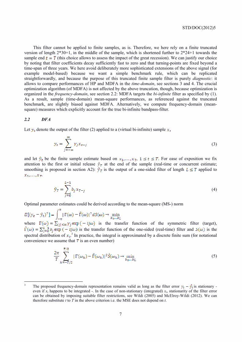
This filter cannot be applied to finite samples, as is. Therefore, we here rely on a finite truncated version of length 2*30+1, in the middle of the sample, which is shortened further to 2*24+1 towards the sample end (this choice allows to assess the impact of the great recession). We can justify our choice by noting that filter coefficients decay sufficiently fast to zero and that turning-points are fixed beyond a time-span of three years. We here avoid deliberately more sophisticated extensions of the above signal (for example model-based) because we want a simple benchmark rule, which can be replicated straightforwardly, and because the purpose of this truncated finite sample filter is purely diagnostic: it allows to compare performances of HP and MDFA in the time-domain, see sections 3 and 4. The crucial optimization algorithm (of MDFA) is not affected by the above truncation, though, because optimization is organized in the frequency-domain, see section 2.2: MDFA targets the bi-infinite filter as specified by (1). As a result, sample (time-domain) mean-square performances, as referenced against the truncated benchmark, are slightly biased against MDFA. Alternatively, we compute frequency-domain (mean-square) measures which explicitly account for the true bi-infinite bandpass-filter.

2.2 DFA

Let denote the output of the filter (2) applied to a (virtual bi-infinite) sample

(3)

and let be the finite sample estimate based on , . For ease of exposition we fix attention to the first or initial release at the end of the sample (real-time or concurrent estimate; smoothing is proposed in section A2): is the output of a one-sided filter of length applied to

.

(4)

Optimal parameter estimates could be derived according to the mean-square (MS-) norm

where is the transfer function of the symmetric filter (target),

is the transfer function of the one-sided (real-time) filter and is the spectral distribution of .3 In practice, the integral is approximated by a discrete finite sum (for notational convenience we assume that is an even number)

(5)

3 The proposed frequency-domain representation remains valid as long as the filter error is stationary -

even if xt happens to be integrated -. In the case of non-stationary (integrated) xt, stationarity of the filter error can be obtained by imposing suitable filter restrictions, see Wildi (2005) and McElroy-Wildi (2012). We can therefore substitute t to T in the above criterion i.e. the MSE does not depend on t.

STD/DOC(2012)5

8

where is an equidistant discrete frequency-grid and is an estimate of the (unknown) spectrum: possible candidates are model-based spectral densities (as obtained by TRAMO or X-12-ARIMA or STAMP, for example) or implicit densities (as assumed implicitly by HP-, CF- or BK-filters, see annex A4) or non-parametric estimates such as the periodogram , see Wildi (2008):

(6)

In this expression, denotes the Discrete Fourier Transform (DFT) of the data :

In contrast to classical maximum likelihood approaches, criterion (5) emphasizes the filter error - not a model residual - and it addresses filter coefficients - not model parameters.

2.3 Shift of Perspective

Before extending the above results to a multivariate framework we briefly emphasize the scope and the shift of perspective entailed by the DFA-criterion (5).

2.3.1 A Generic Approach

Criterion (5) is generic in the sense that the target signal as well as the spectral estimate are neither fixed nor specified in advance by some ‘rule’. In its generic form, the criterion can thus replicate performances of traditional (one-step ahead mean-square) model-based approaches: equate with the model-based spectral density and set (i.e. the target signal becomes a one-step ahead ‘allpass’ filter). A replication of the TRAMO-SEATS4 real-time filter is proposed in McElroy-Wildi (2012), section 6; a replication of TRAMO/SEATS seasonal adjustment filters is proposed in Wildi (2011-e). The generic DFA can also replicate (real-time) performances of classical filters such as HP, see section 4. Whereas simple replication is of no added-value per se, its potential mainly resides in customization, in its ability to modify a particular (replicated) approach, within the generic DFA-framework. We now briefly review this strategy.

2.3.2 Timeliness, Smoothness and Accuracy

This section summarizes results in Wildi (2005), (2008) and Wildi/McElroy (2012). A straightforward application of the law of cosines from trigonometry leads to the following decomposition of the squared transfer function error in (5):

(7)

4 Bank of Spain: http://www.bde.es/webbde/es/secciones/servicio/software/econom.html

STD/DOC(2012)5

9

where and are the amplitude functions (the lengths of the transfer functions in the complex plane) and is the angle between and in the complex plane. Note that for a symmetric strictly positive filter and for the anticipative one-step ahead allpass filter (one-step ahead mean-square optimization). We can now reformulate criterion (5) by inserting (7):

In addition, we can discriminate stopband and passband: the passband PB in our application is and the stopband SB is the difference or complement in :

(8)

(9)

(10)

(11)

The first term (8) is called ‘Accuracy’: it measures the fit of the signal by the asymmetric filter in the passband, irrespective of the induced time- or phase-shift and irrespective of the noise suppression in the stopband. The second term (9) is called ‘Smoothness’: it measures noise suppression by the asymmetric filter in the stop-band. Smaller Smoothness-terms are associated to less noisy - smoother - filter outputs. The third term (10) is called ‘Timeliness’: it measures the contribution of phase-shifts to total MSE in the passband. A larger Timeliness-term is associated with a somehow fuzzy turning-point detection (often turning-points are delayed). The last term (11) is the ‘Residual’: it measures that part of the total MSE which cannot be assigned to the previous three terms. It is generally small because tends to be small in the stopband. In our case it vanishes exactly because the ideal bandpass filter is equal to zero in the stopband.

Measuring the contributions of Timeliness and/or Smoothness terms to total MSE is informative about the quality of the estimate: a large Timeliness-term signifies that turning-points appear systematically shifted (in the filter-output) whereas a large Smoothness term is indicative for unreliable (noisy) detection

STD/DOC(2012)5

10

of turning-points. Therefore, we can rely on this decomposition for diagnostic purposes when evaluating performances of HP and of MDFA, see Sections 3 and 4.

2.3.3 Customization

The above decomposition of ‘total MSE’ into Accuracy, Timeliness and Smoothness terms (plus an irrelevant residual) leads to a natural definition of a trilemma, see McElroy and Wildi (2012).Formally, this three-dimensional tradeoff is obtained by generalizing the MSE-norm to a Customized Criterion:

(12)

where and are initials of the four terms in the above MSE-decomposition and and . For all terms are equally-weighted and the Customized Criterion (12)

replicates the MSE-norm (5). Timeliness could be improved by emphasizing - increasing -, which generally results in ‘faster’ (real-time) filters. Smoothness could be improved by emphasizing - increasing - which results in stronger noise suppression (more reliable real time signals). Obviously, both terms and could be improved simultaneously, at the expense of (and possibly ). Let us emphasize this ‘unorthodox’ outcome by stating that customized (real-time) filters can improve upon traditional mean-square designs in terms of Smoothness as well as Timeliness, simultaneously, see McElroy and Wildi (2012)5, Section 6, for illustration. For diagnostic purposes we shall refer to the decomposition (12) by the alternative denomination AST-trilemma.

2.3.4 Matching DFA and Objectives of the Study

Given the extended scope and the flexibility of the DFA we are in a position to target specific objectives of the study: we here emphasize mean-square performances, we target GDP-BP ‘directly’ (instead of one-step ahead forecasting) and we mark our personal long-term preference for the DFT (instead of model-based or HP-based spectra). Since we want to address full revision sequences, starting in the first release and going all the way up to the final release, the MSE-norm offers a natural and consistent framework for evaluating and assessing performances of competing designs.

2.4 Multivariate Direct Filter Approach (MDFA)

Wildi (2008-m) extends the above results to a multivariate framework, the so-called Multivariate Direct Filter Approach (MDFA). We summarize briefly the main results by considering the stationary case (the case of integrated and/or cointegrated time series is discussed in Wildi (2008-m) and (2011)). Let be the target signal (3) and assume the existence of additional explanatory variables , . We then consider

(13)

5 The authors design a monthly real-time economic indicator for the US. For this purpose they first replicate

signal extraction (trend-) filters of TRAMO/SEATS. In a second step, they customize the replicated model-based real-time filter by augmenting and . They show that the resulting customized filter is both faster (by almost one quarter) and smoother (smaller mean-square curvature) than the original model-based design.

STD/DOC(2012)5

11

where

are the (one-sided) transfer functions applying to the explanatory variables and , are the corresponding DFT’s. Theorem 7.1 in Wildi (2008-m) establishes that the (generalized) criterion

(14)

inherits all efficiency properties of the univariate DFA. The columns of the matrix collect filter-coefficients by series.

Given the extended scope of our generic approach we conclude that MDFA generalizes HP in various crucial aspects: it can target arbitrary signals ‘directly’ (here: GDP-BP), it is data-dependent (by relying on the DFT of the data) and it is truly multivariate (by sensing cross-spectra). We now review performances of the approach when benchmarked against HP and we attempt to decompose and to assign MSE-gains to specific methodological extensions, as offered by MDFA.

We refer to the appendix for a short discussion of smoothing (estimation of for ), filter-constraints and regularization. We also provide closed-form optimization criteria and links to freely available R-code.

3. EMPIRICAL RESULTS: A LOOK ACROSS COUNTRIES

The G7-data used in this study ends in October 2011. Start-dates (sample lengths) depend on the country under scrutiny as well as on the set of selected indicators. In the shortest case (France) we still have approximately 23 years of observations available, when including all relevant indicators, see Gyomai-Wildi (2012). We present here the baseline scenarios, more refined country-specific decompositions of the MSE-norm (AST-trilemma and longitudinal vs. cross-sectional contributions) and an analysis of structural-shifts of filter-coefficients will follow in Section 4. It is important to emphasize that all MDFA results are based on a ‘one-size-fits-all’ (push-the-button) design, as defined in Gyomai and Wildi (2012), section 7.1: MDFA as set-up in this study requires neither country-specific adjustments nor user-interactions of any kind.

3.1 MDFA: Stability-Analysis and Out-of-Sample Performances

In order to verify consistency and stability of MDFA over time, as recessions ‘come and go’, we analyse and compare full-sample as well as out-of-sample mean-square performances. Table (1) summarizes MSEs of concurrent filters (initial releases) against GDP-BP, shifted by the target CLI-lead of 6 months, for full-sample (first column) as well as 4, 10 and 20 years out-of-sample designs (columns 2-4) , across G-7 countries6. A comparison of columns 1 and 2 informs about the effect by the great recession;

6 Two years of data have to be discarded towards the sample end in the implementation of the signal, recall

STD/DOC(2012)5

12

columns 2 and 3 can be used to assess the stability of MDFA during a longer episode without extraordinary events (recessions); the fourth column is mainly intended as a stress-test since estimation samples tend to be very short (less than three years of data available in the case of France, for example).

Table 1. Out-of sample performances: MSEs (and their standard deviation in parenthesis) of concurrent MDFA-filter with respect to GDP-BP shifted by 6 months

2011-10 2007-10 2001-10 1991-10 DEU 0.59 (0.039) 0.63 (0.047) 0.64 (0.05) 0.67 (0.052) FRA 0.36 (0.042) 0.57 (0.081) 0.94 (0.115) 1.1 (0.077) USA 0.41 (0.03) 0.51 (0.036) 0.52 (0.046) 0.55 (0.033) GBR 0.68 (0.107) 0.87 (0.161) 0.86 (0.154) 1.04 (0.175) ITA 0.52 (0.048) 0.69 (0.072) 0.77 (0.081) 1.15 (0.086) CAN 0.59 (0.041) 0.62 (0.038) 0.59 (0.036) 0.7 (0.041) JPN 0.74 (0.059) 0.82 (0.087) 0.83 (0.088) 1.01 (0.077)

Standard deviations, in parentheses, suggest that the effect by the great recession is not significant for Germany, Great-Britain, Canada and Japan. Also, columns 2 and 3 are almost at a tie, except for France and Italy. In column 4 we can see that the performance deteriorates for most countries, but the 20 years out of sample scenario is pushed to extremes and has excessively short estimation samples. Nonetheless, the deterioration in performance is not extreme, and, as we shall see in the coming subsection, it compares well to the overall HP-performance, marking the robustness of MDFA. Based on the out of sample results we conclude that MDFA-performances are stable over longer time spans, at least in the absence of ‘extraordinary’ events, and assuming sufficiently long estimation samples (15 years or more). Extreme events of the magnitude of the great recession appear to have an impact, although statistical significance could not be firmly established for a majority of countries (4 out of 7). We infer that filter coefficients don’t have to be updated frequently. In the absence of extraordinary events, a re-estimation every five years would be sufficient and could be coupled to the regular component reviews of the CLIs, which have similar recurrence. Methodologically, the observed consistency of performances across countries and along the time axis is sustained by regularization7, see Annex A3.

3.2 MDFA vs. HP

MSEs and correlations of initial releases by MDFA and HP are compared in Table (2). All MDFA results refer to the 4-years out-of-sample design whose performances were reported in the second column of Table (1). The comparison of MDFA-performances in the last column of Table (1) with HP-performances reported in Table (2), below, shows that the former still outperforms the latter for most countries.

Section 1. Since the ‘great recession’ ended in the summer of 2009 for the G7 countries (June 2009 for the US; source: NBER dating committee) it is fully embedded in the evaluation sample and its impact can be assessed.

7 The number of effective degrees of freedom is tightly controlled in order to avoid overfitting: for each country, MDFA ‘burns’ only 2-3 degrees of freedom, per series, see Gyomai and Wildi (2012).

STD/DOC(2012)5

13

Table 2. Concurrent filters MDFA vs. HP: MSE’s and correlations when targeting GDP-BP (shifted by 6 months)

MDFA-cor HP-cor MDFA-MSE HP-MSE DEU 0.63 0.12 0.63 1.16 FRA 0.76 0.28 0.57 1.00 USA 0.56 0.12 0.51 0.88 GBR 0.45 0.09 0.87 1.25 ITA 0.64 0.21 0.69 1.15 CAN 0.60 -0.21 0.62 1.13 JPN 0.59 0.09 0.82 1.42

We can observe that MSE efficiency gains by the MDFA are substantial - comprised between and - and that they are consistent over countries which confirms, once again, that performances are stable/robust. In contrast, correlations of initial HP-releases in the second column are often close to zero; in the case of Canada it is even negative.

3.3 Final Releases

Table (3) reviews MSEs and correlations of ‘final releases’ of MDFA and HP. We observe that the ‘final release’ of MDFA is generally much closer to GDP-BP than HP and, accordingly, its correlation is closer to 1, too. Thus the MDFA is not only capable to provide better first estimates of the GDP-BP but also settles closer in the long run to the true target signal. Note that a ‘perfect’ replication of the signal by MDFA could be obtained by including GDP into the set of explanatory data (we currently use the original CLI-data). We notice a considerable improvement from first release to the final release in the case of both methods, but, since final releases of the two approaches markedly differ, a direct comparison of their revision-sequences may be misleading. We defer the analysis of revisions paths to Section 5, where we tune the MDFA estimates to converge to the final HP-CLI outcomes rather than the GDP-BP, thus allowing consistent direct comparisons.

Table 3. Final Release MDFA vs. HP: MSE’s and correlations when targeting GDP-BP (shifted by 6 months)

MDFA-cor HP-cor MDFA-MSE HP-MSE DEU 0.95 0.72 0.18 0.50 FRA 0.96 0.80 0.17 0.41 USA 0.93 0.84 0.19 0.39 GBR 0.86 0.68 0.43 0.56 ITA 0.88 0.71 0.23 0.51 CAN 0.95 0.52 0.13 0.63 JPN 0.93 0.74 0.17 0.49

3.4 Origins of Efficiency Gains

To analyze the origins of efficiency gains first we construct a new filter, called MDFA-uniform, whose coefficients are fixed across time series8 - like the HP-filter’s are by design. This enables us to allocate filter improvements brought by the MDFA to longitudinal and cross-sectional elements. A comparison of HP and MDFA-uniform informs about efficiency gains attributable to better longitudinal (fixed-coefficient) filtering whereas a comparison of MDFA-uniform and MDFA quantifies partial benefits obtained by relaxing the fixed-coefficient restriction. The effectiveness of the approach is illustrated for Germany in Fig.5: filter-coefficients and spectral outputs are now virtually indistinguishable across time series, in contrast to Figs.1-4 for the unrestricted design.

8 MDFA uniform is obtained by setting in the Regularization-Troika 28, see Gyomai-Wildi (2012)

for reference.

STD/DOC(2012)5

14

Table 4. First release values performance with the HP-filter, the MDFA, and the constrained MDFA (forcing uniform weights across series, only allowing longitudinal effects)

Correlation MSE MDFA MDFA

uniform HP MDFA MDFA

uniform HP

DEU 0.63 0.35 0.12 0.63 0.84 1.16 USA 0.56 0.44 0.12 0.51 0.53 0.88 FRA 0.76 0.43 0.28 0.57 0.83 1.00 GBR 0.45 0.22 0.09 0.87 1.00 1.25 ITA 0.64 0.33 0.21 0.69 0.90 1.15 CAN 0.60 0.44 -0.21 0.62 0.69 1.13 JPN 0.59 0.51 0.09 0.82 0.92 1.42

A decomposition of total MSEs and correlations into longitudinal and cross-sectional components, through MDFA-uniform, suggests that for the majority of the countries the longitudinal improvements dominate (more than 70% of MSE improvement is attributable to longitudinal effects). Nonetheless for a few countries the cross-sectional improvements are equally important. See Table 4 above.

In a second step origins of efficiency gains are assessed in the frequency-domain, according to the MSE-decomposition presented in Section 2.3.2, see Annex A5 for further details.

Table 5. Frequency domain MSE components by (A) Accuracy, (S) Smoothness, (T) Timeliness.

MDFA HP A S T Total A S T Total DEU 0.26 0.01 0.20 0.46 0.09 0.03 0.86 0.99 FRA 0.17 0.00 0.04 0.22 0.05 0.02 0.78 0.85 USA 0.31 0.01 0.20 0.53 0.14 0.03 1.07 1.24 GBR 0.05 0.00 0.04 0.10 0.08 0.03 0.74 0.85 ITA 0.34 0.00 0.13 0.47 0.15 0.02 1.11 1.28 CAN 0.34 0.01 0.16 0.51 0.17 0.04 1.46 1.68 JPN 0.27 0.00 0.10 0.37 0.23 0.01 1.01 1.26

Please note that frequency-domain MSEs differ from their time-domain counterparts.

The results are shown for the 4-years out-of-sample MDFA-design and the HP-filter. We note that (frequency-domain) MSEs of MDFA and of HP differ somewhat from the corresponding sample MSEs reported in Table (2) which is attributable, in part, to the fact that the sample-period in Table (5) ends in Oct-2007 and does not cover the great recession (whereas sample MSEs in Table (2) do). The magnitude of MDFA efficiency-gains in the frequency-domain ranges between - whereas the time-domain efficiency-gains range - , and although the ranges are different, they both signal substantial efficiency-gains achievable with the MDFA compared to the HP-filter. Further scrutiny of the AST breakdowns shows that the MDFA ‘splits’ mean-square contributions more or less evenly across Accuracy and Timeliness terms, with slightly higher share falling on the Accuracy term. In contrast, the HP-filter often performs better in terms of Accuracy at the expense of Timeliness: the poorer Timeliness properties determine entirely the loss in efficiency by the HP-filter’s real-time performance. This result is relevant in the sense that the Timeliness-component of the MSE-norm is closely related to the dating of turning-points. This means that initial turning-point reading from the HP-filter should be handled cautiously, and Fig. 7 suggests that the final release by HP may still have timeliness related errors and cannot always track turning-points of GDP-BP well.

STD/DOC(2012)5

15

4. EMPIRICAL RESULTS: A DETAILED COUNTRY-SPECIFIC ANALYSIS

As we could see, the results are fairly consistent across countries. In this section we have chosen one country to present further in-depth analysis that we have carried out, but that would be difficult to summarize for all G7 countries. For illustration we have selected Germany; nonetheless results for the remaining G7 countries can be found in a more complete report: Gyomai and Wildi (2012), Chapter 4. In this section we provide additional out-of-sample (stability) analysis and we investigate the full revision-sequence for Germany.

4.1 Stability-Analysis: Structural-Shifts in MDFA’s Filter Coefficients

Figures 1-4 complement the out-sample results reported in Table (1) by an analysis of filter coefficients (bottom graphs) and filter-outputs (top graphs)9 for full-sample as well as 4, 10 and 20-years out-of-sample MDFA-designs. A graphical analysis of systematic structural shifts in coefficients and/or in spectra can be useful when monitoring a CLI dynamically, as time evolves, or when assessing the importance of current data or of new potentially interesting candidates.

The CLI for Germany consists of 6 components, coded as follows in Figures 1-5. • LOCOBDOR – Orders Inflow – tendency, (red) • LOCOBFOR – Finished Good Stocks – tendency (yellow) • LOCOBSOR – Business Climate Indicator (green) • LOCOBXOR – Export Order Books – tendency (light-blue) • LOCOODOR – New Orders in manufacturing (dark-blue) • LOCOSIOR – Spread of Interest Rates (violet)

9 We plot for each series the periodogram of the output of the corresponding (MDFA) sub-filter: ideally, we

expect the spectral content to be ‘large’ (in relative terms) in the assigned passband (2-10 years, or between frequencies π/60 and π/12) and to be ‘small’ in the stop-band (assuming that components in the stop-band are not perfectly cross-correlated). Dominant spectral power of a particular series signifies that it contributes substantially to the (aggregated) MDFA estimate.

STD/DOC(2012)5

16

Figure 1. Germany - MDFA based on a sample period from 1969-01 to 2011-10. Spectral power of series-specific filter outputs (top) and filter coefficients (bottom): filter length (per series) is 61.

Figure 2. Germany - MDFA based on a sample period from 1969-01 to 2007-10. Spectral power of series-specific filter outputs (top) and filter coefficients (bottom): filter length (per series) is 61.

STD/DOC(2012)5

17

Figure 3. Germany - MDFA based on sample period from 1969-01 to 2001-10. Spectral power of series-specific filter outputs (top) and filter coefficients (bottom): filter length (per series) is 61.

Figure 4. Germany - MDFA based on sample period from 1969-01 to 1991-10. Spectral power of series-specific filter outputs (top) and filter coefficients (bottom): filter length (per series) is 61.

STD/DOC(2012)5

18

Figure 5. Germany - MDFA constrained to have the same filter coefficients across components. Spectral power of series specific filter outputs (top) and filter coefficients (bottom).

The most notable development over the years is that Export order books (series LOCOBXOR) gradually gains in importance and the spread of interest rates (LOCOSIOR) gradually looses in importance over time. The footprint by the great recession is heftier and less gradual but it is in-line with the historical tendency. The negative filter coefficients observed in the case of the spread of interest rate components, suggests a countercyclical behavior – this information is automatically picked up by the MDFA, whereas it has to be specified in the case of the HP-filter. Finally, Fig. 5 above illustrates the impact of constraining the filter weights to be alike across components, i.e. demonstrating the MDFA-uniform’s filter coefficients and filter outputs.

4.2 Revision Sequence

Fig.7 compares final releases of HP and MDFA with GDP-BP. The latter tracks turning-points of the signal better, which was rewarded by a larger correlation ( ) in Table (3). The strong final correlation of the MDFA suggests, in turn, that the morphism along its revision sequence could be marked, i.e. individual revisions may be larger as the filtered series adjusts to get closer and closer to the target, see Fig.810. At the same time the HP-filter revisions sweep a narrower range, but this comes together with HP’s inability to closely follow the GDP-BP target, its final correlation with GDP-BP being only ( ). Columns 2 and 4 in Table (7) try to capture the difference in morphism through presenting correlations to own final estimates of consecutive HP and MDFA filtered values. However as final releases of the two approaches differ substantially, we refer to Section 5 for a formally consistent, direct comparison of revision-paths and a discussion of convergence issues.

Tables (6) and (7) report MSEs and correlations along the full revision-sequence (we report results for filter-variants between 6 months lead and 23 months lag because at 23 months lag in the current framework 10 The filtered time series start with a lag of 5 years because we imposed a filter length of 61 (months).

STD/DOC(2012)5

19

the HP-filters become fully symmetric and their values are regarded as final after 30 months). Fig. 6 provides a convenient graphical summary of the two tables. The MSE-numbers collected in Table (6) are organized according to three different designs: ordinary MSEs (as reported in all previous tables), ‘scaled’ measures (we divided MSEs by the variance of the signal) and ‘standardized’ measures (MSEs are computed between standardized estimates and standardized signal). The last two measures are easy to interpret: if the MSE exceeds one, then the filter would be outperformed by a constant. Also, the last (standardized) measure allows disentangling bias and variance contributions to total MSE.

Correlations tend to augment and MSEs tend to decay with decreasing lead or increasing lag. We expect a monotonic pattern because higher-lag estimates can rely on ‘future’ information which is hidden to smaller-lag/higher-lead filters: remarkably, this progression is not always perfectly monotonic in the case of HP, and is attributable to the non-optimizing nature of the filter, as filter misspecifications are not eliminated in the calibration phase and can manifest themselves in non-monotonic behaviour; see Gyomai and Wildi (2012) for further discussion11. Even disregarding the minor monotony flaw of the HP-filter, Fig.6 confirms the uniformly better performance by MDFA; in particular, HP cannot provide better estimates than the initial release of MDFA before a lag-time of 9 months (the blue lines in both the MSE- and correlation-graphs cross the black horizontal lines in lag=9). This means that the initial release of MDFA has a comparable performance to the 16th vintage of the HP-filtered estimate (note that in the current exercise the first, real-time vintage is providing a 6 months lead, so the value at 9 months lag corresponds to the 16th vintage). This remarkable result is fairly consistent across countries; see Gyomai-Wildi (2012).

Figure 6. Germany - MSEs (top) and correlations (bottom) of MDFA (blue) and HP (red) as a function of leads/lags when targeting GDP-BP

11 The HP-filter is subject to a severe unit-root misspecification since it is inherently designed for I(2)-series. In

contrast, MDFA assumes stationarity, see McElroy and Wildi (2012) section 6 for a similar unit-root conflict opposing (univariate) DFA to TRAMO/SEATS (with a similar outcome).

STD/DOC(2012)5

20

Figure 7. Germany - Final estimates of the MDFA (green) and HP-based CLI (violet) vs. target GDP-BP (red)

Figure 8. Germany - Revision sequence of MDFA: GDP-BP is targeted

STD/DOC(2012)5

21

Table 6. Germany: MSE’s of successive releases of MDFA and HP referenced against GDP-BP. No transformation (columns 1 and 4), scaling of previous MSE by inverse of variance of signal (columns 2 and 5),

MSE between standardized signals (columns 3 and 6)

MDFA MDFA scaled MDFA stand. HP HP scaled HP stand. Lag -6 0.63 0.67 0.74 1.16 1.24 1.76 Lag -5 0.62 0.66 0.72 1.18 1.26 1.79 Lag -4 0.61 0.65 0.71 1.19 1.28 1.81 Lag -3 0.60 0.64 0.70 1.21 1.29 1.83 Lag -2 0.60 0.64 0.70 1.21 1.29 1.83 Lag -1 0.59 0.63 0.69 1.21 1.28 1.82 Lag 0 0.59 0.62 0.69 1.18 1.24 1.77 Lag 1 0.58 0.61 0.67 1.13 1.19 1.69 Lag 2 0.57 0.59 0.65 1.08 1.12 1.58 Lag 3 0.55 0.57 0.63 1.01 1.04 1.45 Lag 4 0.53 0.54 0.60 0.95 0.97 1.32 Lag 5 0.51 0.51 0.56 0.88 0.89 1.20 Lag 6 0.48 0.48 0.52 0.82 0.82 1.09

… Lag 22 0.18 0.18 0.10 0.49 0.49 0.56 Lag 23 0.18 0.18 0.10 0.50 0.49 0.57

Table 7. Germany: Correlation of successive releases of MDFA and HP referenced against GDP-BP (columns

1 and 3) and final releases (columns 2 and 4)

MDFA/GDP-BP MDFA/final release HP/GDP-BP HP/final release Lag -6 0.63 0.67 0.12 0.71 Lag -5 0.64 0.68 0.10 0.70 Lag -4 0.64 0.69 0.09 0.68 Lag -3 0.65 0.69 0.08 0.67 Lag -2 0.65 0.70 0.08 0.66 Lag -1 0.65 0.70 0.09 0.68 Lag 0 0.66 0.71 0.11 0.70 Lag 1 0.66 0.72 0.15 0.74 Lag 2 0.67 0.73 0.21 0.78 Lag 3 0.68 0.75 0.27 0.81 Lag 4 0.70 0.76 0.34 0.84 Lag 5 0.72 0.78 0.40 0.86 Lag 6 0.74 0.81 0.46 0.88

… Lag 22 0.95 1.00 0.72 1.00 Lag 23 0.95 1.00 0.72 1.00

5. MDFA TO REPLICATE THE HP-BASED CLI

In contrast to the previous sections we propose here to target the final release of HP by MDFA: the resulting design is called MDFA-CLI. It can be obtained very easily by inserting the DFT (Discrete Fourier Transform) of the final HP-based release into (5) or (14)12. For the moment, in this scenario, we drop the GDP-BP as a target to concentrate on revision patterns. Our motivation here is twofold:

1. In contrast to the previous MDFA, the new MDFA-CLI and HP share a common target, namely the (aggregated) output of the symmetric HP-filter. Therefore convergence of revision-sequences

12 is identified with the DFT of the CLI’s.

STD/DOC(2012)5

22

- towards final estimates - and consistency or stability of early turning-point signals can be compared directly.

2. Final-HP is ‘easier’ to approximate than GDP-BP (the information base for the target and the MDFA is the same) and therefore revisions of MDFA-CLI are smaller when referenced against the new target. This advantage of the new MDFA-CLI over the previous MDFA could be appealing to analysts prioritizing small revisions and stable real-time figures over tight GDP-BP approximation. Suitable linear combinations of both designs could lead to some ‘optimal’ compromise between these conflicting requirements.

Table (8) compares MSEs and correlations of MDFA-CLI and HP when referenced against HP-final: Fig.9 provides a convenient graphical summary of these numbers13. We notice, once again, a non-monotonic pattern in successive HP-releases up to lag 4. The table reveals a strong correlation of the initial release of MDFA-CLI ( ) with the new target and a gain in efficiency, over HP, of

whose magnitude is remarkable given that HP is referenced against its own final release. Revisions of MDFA-CLI are smaller and convergence is faster 14. Please note that comparisons towards the sample-end in these figures are more or less strongly biased in favor of HP because the target signal (HP-final) becomes more and more asymmetric i.e. real-time HP and final-HP coincide towards . Fig. 11, as compared to Fig 8., shows how much the revisions decrease when the target series is constructed from a similar information set to the, and this suggests that the inclusion of the historical GDP series could further improve the MDFA design.

Figure 9. Germany - MSEs (top) and correlations (bottom) of MDFA (blue) and HP (red) as a function of leads/lags when targeting the CLI

13 Since HP-final is already leading we do not impose an extra-lead i.e. the table ‘starts’ with Lag 0 (instead of

Lag -6 in the case of GDP-BP). 14 The lag(24) MSE for MDFA-CLI (0.02) is slightly larger than HP (0.01) because of arbitrary filter-length

settings and finite-sample scaling issues. These differences are negligible by all practical means.

STD/DOC(2012)5

23

Figure 11. Germany - Revision sequence MDFA-CLI: HP-final is targeted

Figure 10. Germany - Real-time (Lag 0) MDFA-CLI vs. real-time HP targeting HP-final

STD/DOC(2012)5

24

Table 8. Germany MSEs and correlations of successive releases of MDFA and HP referenced against HP-final

MDFA: MSE HP: MSE MDFA: corr HP: corr Lag 0 0.10 0.28 0.94 0.71 Lag 1 0.09 0.29 0.94 0.70 Lag 2 0.08 0.31 0.95 0.68 Lag 3 0.08 0.32 0.95 0.67 Lag 4 0.08 0.32 0.95 0.66 Lag 5 0.08 0.31 0.95 0.68 Lag 6 0.08 0.28 0.95 0.70

… Lag 21 0.02 0.02 0.99 0.98 Lag 22 0.02 0.01 0.99 0.99 Lag 23 0.02 0.01 0.99 0.99 Lag 24 0.02 0.01 0.99 1.00

6. SUMMARY

We benchmarked real-time performances and convergence of revision-sequences of a MDFA-design against HP, when referenced to GDP-BP for G7-countries. Efficiency gains of MDFA are substantial across G7 countries and they are consistent over time: we observe a reduction of MSEs of initial release by MDFA (over HP) comprised between and if estimation samples are sufficiently long (15-20 years of data depending on the country under scrutiny), or otherwise put, the real-time MDFA results are as good as HP-filter based estimated after 15 months. MDFA does not require frequent updating of filter coefficients because absolute and relative out-of-sample performances are stable over long time spans in the absence of extreme recessions. We have found that extraordinary events of the caliber of the great recession can have significant impacts at least for three out of seven countries - USA, France and Italy - and our results also suggest that MDFA-performances for France needed some time to settle-in. For these countries we recommend a regular monitoring of performances and a graphical analysis of potential structural-shifts of coefficients across time series. The recommended 5-annual frequency for filter reviews coincides with the frequency of component reviews in the current OECD CLI system, therefore would not induce excess volatility and revisions compared to the current operations.

HP mainly looses in terms of Timeliness which suggests that real-time ‘dating’ of turning-points by HP is subject to biases, when referenced against GDP-BP. A larger part efficiency gains by MDFA can be attributed to better longitudinal filtering whereas the remaining part is obtained by effective multivariate filtering. These results vary somewhat from country to country, but in general the study demonstrates, that MDFA can efficiently utilize both the longitudinal and multivariate information of the components of the CLI.

The MDFA is more versatile than the HP-filter, the extra flexibilities allow envisaging various scenarios that would be difficult or impossible to implement with the HP-filter. We have seen how it can better replicate the final HP-filter signal than the HP-filter itself. This could lead to a system in which the departure from the current HP-filtered CLIs towards the pure MDFA-based is gradual, by mixing the two MDFA signals with different targets. But the scope is even wider: the GDP figures (with their typical lags) could also be added to the MDFA information base, and the filter would gradually increase the weight of GDP until perfect convergence, or the filter optimization could be fine tuned to a different balance between accuracy, timing-errors, and smoothness.

STD/DOC(2012)5

25

ANNEX

SMOOTHING, CUSTOMIZATION, REGULARIZATION, OPTIMIZATION CRITERIA FOR MDFA AND REPLICATION OF HP

A1. Optimization Criterion

We first rewrite the MDFA-optimization criterion proposed in section 2.4

(15)

in a more convenient way. Let be the sample-size, be the filter length and be the number of explaining series: as well as , . We then define a -dimensional design-matrix whose -th row is obtained from appending the rows in the following matrix to a (possibly very long) row-vector:

(16)

The -operator appends rows (we use this notation in order to avoid margin-overflow). The dimension of is : the -row corresponds to frequency , in 1 (negative frequencies can be ignored due to symmetry15). Define as the vector of (stacked) filter coefficients

The operator in this expression stacks columns. Finally, define the vector of ‘dependent’ variables by

By neglecting the constant in (15), we can now express the optimization criterion in the more familiar form

15 For notational simplicity we ignored the fact that frequency zero appears once only, whereas all other

frequencies are mirrored and thus appear twice. Indeed, we can ignore this issue because transfer functions of bandpass-filters vanish in frequency zero such that the potential error is avoided, anyway. Exact expressions are proposed in Wildi (2012).

STD/DOC(2012)5

26

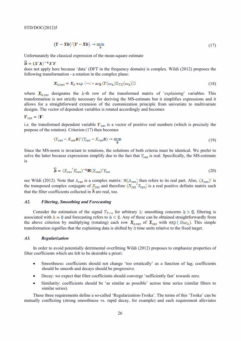
(17)

Unfortunately the classical expression of the mean-square estimate

does not apply here because ‘data’ (DFT in the frequency domain) is complex. Wildi (2012) proposes the following transformation - a rotation in the complex plane:

(18)

where designates the -th row of the transformed matrix of ‘explaining’ variables. This transformation is not strictly necessary for deriving the MS-estimate but it simplifies expressions and it allows for a straightforward extension of the customization principle from univariate to multivariate designs. The vector of dependent variables is rotated accordingly and becomes

i.e. the transformed dependent variable is a vector of positive real numbers (which is precisely the purpose of the rotation). Criterion (17) then becomes

(19)

Since the MS-norm is invariant to rotations, the solutions of both criteria must be identical. We prefer to solve the latter because expressions simplify due to the fact that is real. Specifically, the MS-estimate is

(20)

see Wildi (2012). Note that is a complex matrix: then refers to its real part. Also, is the transposed complex conjugate of and therefore is a real positive definite matrix such that the filter coefficients collected in are real, too.

A2. Filtering, Smoothing and Forecasting

Consider the estimation of the signal for arbitrary : smoothing concerns , filtering is associated with and forecasting refers to . Any of these can be obtained straightforwardly from the above criterion by multiplying (rotating) each row of with . This simple transformation signifies that the explaining data is shifted by time units relative to the fixed target.

A3. Regularization

In order to avoid potentially detrimental overfitting Wildi (2012) proposes to emphasize properties of filter coefficients which are felt to be desirable a priori:

• Smoothness: coefficients should not change ‘too erratically’ as a function of lag; coefficients should be smooth and decays should be progressive.

• Decay: we expect that filter coefficients should converge ‘sufficiently fast’ towards zero. • Similarity: coefficients should be ‘as similar as possible’ across time series (similar filters to

similar series). These three requirements define a so-called ‘Regularization-Troika’. The terms of this ‘Troika’ can be

mutually conflicting (strong smoothness vs. rapid decay, for example) and each requirement alleviates

STD/DOC(2012)5

27

overfitting by highlighting desirable coefficient patterns. Wildi (2012) collects the three terms of the Troika into a single optimization criterion which generalizes (19):

(21)

The matrices , and define positive definite bilinear forms. We here briefly review the ‘smoothing’-part and refer the interested reader to Wildi (2012) and Gyomai-Wildi (2012) for a definition of and .

where is a matrix. It is not difficult (but cumbersome) to show that

(22)

where denote second-order differences. Therefore is a measure for the quadratic curvature - smoothness - of filter coefficients: if coefficients decay linearly, as a function of the lag, then this term vanishes. Increasing in (21) will assign preference to MDFA solutions whose coefficients evolve smoothly as a function of lag: in the limit, when , filter coefficients mustbe linear (as a function of the lag). The solution of the regularized criterion (21) is given by:

(23)

where the super-script ‘Reg’ signifies regularization, see Wildi (2012) for details of this derivation. Note that (23) simplifies to (20) if no regularization is imposed: . Our ‘push-the-button’ MDFA-design is based on empirically approved settings for these parameters16:

and . The number of effectively estimated ‘parameters’ shrinks from 61 (which corresponds to the filter length ), in the absence of regularization, to below 3, per series. MDFA-cross, whose coefficients are fixed across countries, is obtained by imposing a ‘large’

in (23), instead of in the case of MDFA17

16 The regularization-setting is borrowed from the EURI (http://www.idp.zhaw.ch/euri) without additional

adjustments i.e. it is truly ‘out-of-sample’. 17 The interested reader can find a tutorial with R-code and exercises illustrating the various effects of the

STD/DOC(2012)5

28

A4. MDFA and the Hodrick-Prescott Filter

As stated in section 2.2 MDFA is a generic approach. To illustrate the topic we can replicate HP by DFA (univariate MDFA). For this purpose we rely on McElroy (2008), Maravall-Kaiser (1999) and Mise et al. (2003). Specifically, these authors derive the HP-filter by postulating an IMA(2,2)-process for in (3):

The MA-coefficients are determined by the smoothing parameter of the HP-design: McElroy (2008) derives exact formulas

where . Under this IMA(2,2)-specification for the HP-filter solves a classical Wiener-Kolmogorov (mean-square) signal-extraction problem, see Maravall-Kaiser (1999) and McElroy (2008). In the generic DFA-framework this problem can be replicated by plugging the (bi-infinite) symmetric HP-trend filter

(see McElroy (2008), section 2) and the pseudo-spectral density of the implicit IMA(2,2)-representation of the data

into (5). In order to avoid singularities, due to the double unit-root of the hypothetical IMA(2,2)-assumption, one has to impose first and second order filter constraints in frequency zero: these constraints ensure that the signal and the real-time estimate are cointegrated or, equivalently, that the revision error variance is finite. The interested reader is referred to a tutorial on SEFBlog18 which covers the topic.

A5. Assessing Timeliness, Smoothness and Accuracy Terms for the HP-Filter

Consider the (equally-weighted) decomposition of the mean-square filter error presented in section 2.3.3:

where and and are initials for Accuracy, Smoothness, Timeliness and Residual terms introduced in section 2.3.2 (note that in our case because the amplitude function of the ideal bandpass filter vanishes in the stop-band). The equally-weighted scheme emphasizes that we are interested in tracking mean-square performances. and can be inferred

Regularization Troika on SEFBlog: http://blog.zhaw.ch/idp/sefblog/index.php?/archives/246-Live-Tutorial-Round-2-What-is-Regularization-A-Follow-UP.html

18 R-Code, for replicating HP, and instructions, for replicating the example, are provided: http://blog.zhaw.ch/idp/sefblog/index.php?/archives/261-Replication-of-the-Hodrick-Prescott-Filter-by-I-MDFA.html

STD/DOC(2012)5

29

straightforwardly for MDFA, as a natural outcome of the optimization procedure. But the above universal decomposition - trilemma - applies naturally to alternative approaches too. To illustrate the topic, we assume that denotes the transfunction of the concurrent HP-filter ( ). We then plug

and into (8), (9) and (10) to obtain and , say. Note that the target has been specified in (1): since the filter is symmetric and positive

everywhere and . Last but not least, the frequency-domain -estimate is the sum of these three terms (since theresidual vanishes). These numbers - diagnostics - for the HP-filter were reported in Table (5).

STD/DOC(2012)5

30

REFERENCES

[1] McElroy, T. (2008). Exact Formulas for the Hodrick-Prescott Filter. Econometrics Journal , 1–9.

[2] McElroy, T. and Wildi, M. (2010). Signal Extraction Revision Variances as a Goodness-of-Fit Measure. Journal of Time Series Econometrics , Iss. 1, Article 4.

[3] McElroy, T. and Wildi, M. (2012) Multi-Step Ahead Estimation of Time Series Models. Submitted to International Journal of Forecasting.

http://blog.zhaw.ch/idp/sefblog/index.php?/archives/169-Multi-Step-Ahead-Forecasting-Work-with-Tucker-McElroy-Recent-2010-Publication-and-Work-in-Progress.html

[4] McElroy, T. and Wildi, M. (2012) On a Trilemma Between Accuracy, Timeliness and Smoothness in Real-Time Forecasting and Signal Extraction. Submitted to International Journal of Forecasting.

http://blog.zhaw.ch/idp/sefblog/index.php?/archives/263-On-a-Trilemma-Between-Accuracy,-Timeliness-and-Smoothness-in-Real-Time-Forecasting-and-Signal-Extraction.html

[5] Mise E. and Kim T.H. and Newbold P. (2003).On suboptimality of the Hodrick-Prescott filter at time series endpoints. Journal of Macroeconomics 27 (2005) 53-67.

[6] Nilsson R. and Gyomai G. (2011). Cycle Extraction: A Comparison of the Phase-Average Trend Method, the Hodrick-Prescott and Christiano-Fitzgerald Filters. OECD Statistics Working Papers 2011/4, OECD Publishing.

[7] Gyomai G. and Guidetti E. (2012). OECD System of Composite Leading Indicators. methodological manual: http://www.oecd.org/dataoecd/26/39/41629509.pdf

[8] Fulop G. and Gyomai G. (2012). Transition of the OECD CLI system to a GDP-based business cycle target. report: http://www.oecd.org/dataoecd/35/27/49985449.pdf

[9] Gyomai G. and Wildi M. (2012). Report on the Comparison of the Hodrick-Prescott Filter and the Multivariate Direct Filter Approach in Composite Leading Indicators Construction. A case for G7 Countries. OECD research-report,

http://www.oecd.org/std/leadingindicatorsandtendencysurveys/Wildi-Gyomai%20CLI%20report%202012.pdf

[10] Orphanides A. and van Norden S. (2002). The unreliability of output-gap estimates in real time. The Review of Economics and Statistics, Vol. 84(4), pp. 569-583.

[11] Wildi, M. (1998) Detection of Compatible Turning Points and Signal Extraction for Non- Stationary Time Series. Operation Research Proceedings, Springer.

[12] Wildi, M. (2005) Signal Extraction: Efficient Estimation, Unit-Root Tests and Early detection of Turning Points. Lecture Notes in Economics and Mathematical Systems, 547: Springer.

STD/DOC(2012)5

31

[13] Wildi, M. (2008) Real-Time Signal Extraction: Beyond Maximum Likelihood Principles. Berlin: Springer. http://blog.zhaw.ch/idp/sefblog/index.php?/archives/168-RTSE-My-Good-Old-Book.html

[14] Wildi, M. (2008-m). Efficient multivariate real-time filtering and cointegration. Idp-working paper, idp-wp-08sep- 01, Institute of Data Analysis and Process Design, ZHAW. http://www.idp.zhaw.ch/fileadmin/user upload/engineering/ Institute und Zentren/IDP/forschungsschwerpunkte/FRME/sef/signalextraction/papers/IDP-WP-08Sep-01.pdf

[15] Wildi, M. (2010) Real-Time Signal Extraction: a Shift of Perspective. Estudios de Economia Aplicada, vol. 28, num. 3, 2010, pp. 497-518

http://redalyc.uaemex.mx/redalyc/pdf/301/30120334001.pdf

[16] Wildi, M. (2011) A Unified Framework to Real-Time Signal Extraction and Data Revisions. http://blog.zhaw.ch/idp/sefblog/index.php?/archives/163-A-Unified-Framework-to-Real-Time-Signal-Extraction-RTSE-and-Data-Revisions.html

[17] Wildi, M. (2011-e) Real Time Trend Extraction and Seasonal Adjustment: a Generalized Direct Filter Approach. Principal European Economic Indicators (PEEIs) - Lot 2: Advanced statistical and econometric techniques for PEEIs.

[18] Wildi, M. (2012) Elements of Forecasting and Signal Extraction. http://blog.zhaw.ch/idp/sefblog/index.php?/archives/259-Elements-of-Forecasting-and-Signal-

Extraction.html