qual doc spil-1 2012
TRANSCRIPT
Quality Documentation
May 2021
Proficiency test SPIL-1 (2021) Organic matter, phosphorus, chloride, sulphate and suspended matter in wastewater (effluent)
Proficiency test SPIL-1 (2021) Quality Documentation May 2021
Eurofins Miljø A/S Smedeskovvej 38 DK-8464 Galten Denmark Tlf: +45 7022 4266
e-mail: [email protected]
Web: www.eurofins.dk
Client
Environmental laboratories
Client’s representative
Project
Proficiency test SPIL-1 (2021)
Project No
20405-11
Authors
Rikke Mikkelsen
Date 2021-05-20
Approved by Peter Rerup
1 Quality Documentation Report FYE3 PRE PRE 2021-05-25
Revision Description By Checked Approved Date
Key words
Analytical quality, assigned value, precision, trueness, homogeneity, stability, CODCr, BOD5 (w. ATU), BOD7 (w. ATU), NVOC/TOC, total phosphorus, chloride, sulphate, suspended matter, wastewater
Classification
Open
Internal
Proprietary
Distribution
Available online: Eurofins:
www.eurofins.dk Rikke Mikkelsen, Peter Rerup
CONTENTS
1 INTRODUCTION ........................................................................................................... 1
2 FEATURES OF THE PROFICIENCY TEST .................................................................. 2
2.1 Sample preparation ....................................................................................................... 2
2.2 Statistical analysis of participants’ data ......................................................................... 2 2.3 Assigned and spike value .............................................................................................. 2
2.3.1 Assigned and spike values ............................................................................................ 3
2.3.2 Test of spike values ...................................................................................................... 3 2.3.3 Test of assigned values ................................................................................................. 4
3 HOMOGENEITY AND STABILITY OF SAMPLES ......................................................... 5
4 CONCLUSION .............................................................................................................. 6
5 REFERENCES ............................................................................................................. 7
ANNEX A LIST OF PARTICIPANTS ..................................................................................... 9
ANNEX B SAMPLE PREPARATION .................................................................................. 11
ANNEX C CONTROL OF SPIKE VALUES ......................................................................... 13
ANNEX D CONTROL OF RECOVERY ............................................................................... 21
ANNEX E CONCENTRATION LEVEL ................................................................................ 29
ANNEX F HOMOGENEITY AND STABILITY ..................................................................... 30
Page 1 of 32
1 INTRODUCTION
A proficiency test on the analysis of organic matter, phosphorus, chloride, sulphate and suspended matter in wastewater was conducted on 11 Marts 2021. The proficiency test was organised by Eurofins Miljø A/S.
The present report contains Eurofins’ documentation for the quality of the proficiency test. Results of the proficiency test including data from participating laboratories and sta-tistical analysis of these data were issued in a report to all participants /1/ on 13 April 2021.
Page 2 of 32
2 FEATURES OF THE PROFICIENCY TEST
Participants in the proficiency test were a total of 54 laboratories from Denmark, Ger-many, Norway and Sweden. A list of participants is shown in Appendix A.
The closing date for submission of results was 26 March 2021. All participants had sub-mitted their results before the dead-line.
2.1 Sample preparation
The parameters covered in the proficiency test are listed in Table 2 as are the abbrevia-tions used in this report.
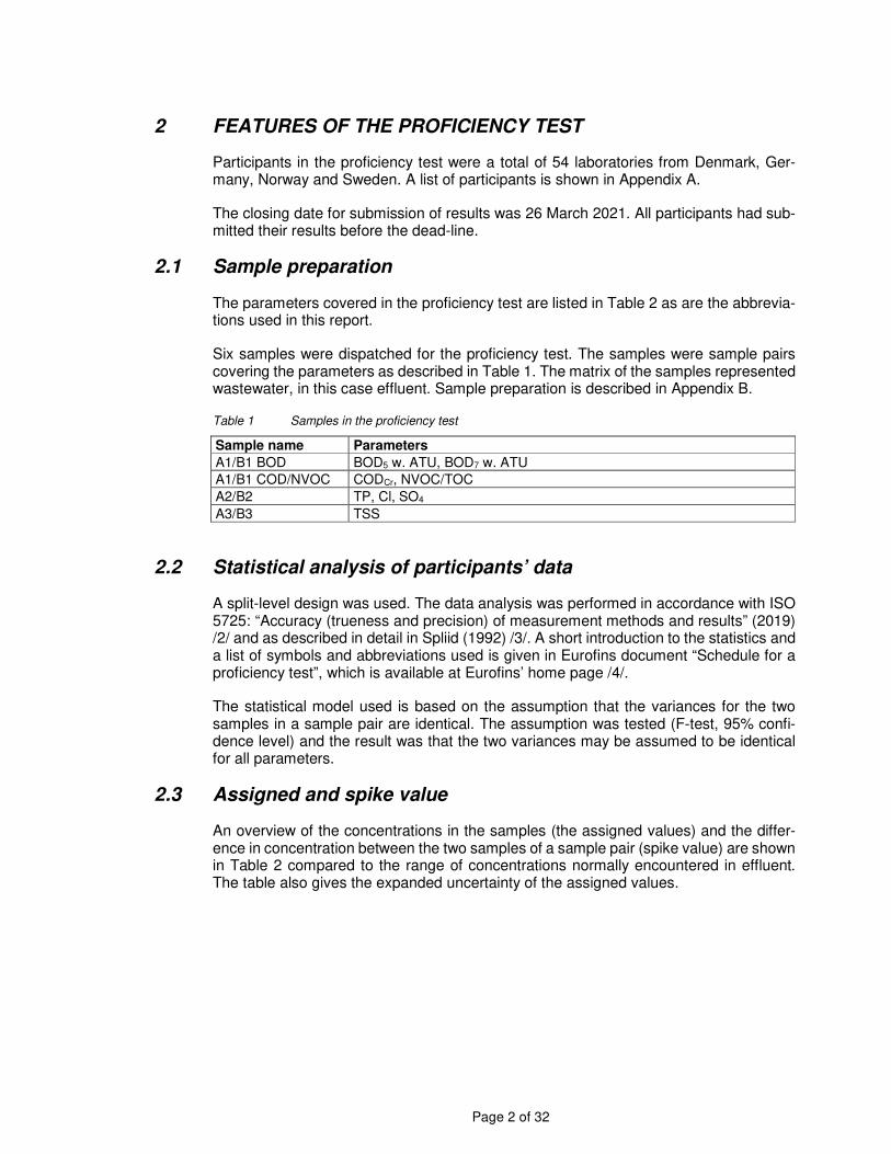
Six samples were dispatched for the proficiency test. The samples were sample pairs covering the parameters as described in Table 1. The matrix of the samples represented wastewater, in this case effluent. Sample preparation is described in Appendix B.
Table 1 Samples in the proficiency test
Sample name Parameters
A1/B1 BOD BOD5 w. ATU, BOD7 w. ATU A1/B1 COD/NVOC CODCr, NVOC/TOC A2/B2 TP, Cl, SO4 A3/B3 TSS
2.2 Statistical analysis of participants’ data
A split-level design was used. The data analysis was performed in accordance with ISO 5725: “Accuracy (trueness and precision) of measurement methods and results” (2019) /2/ and as described in detail in Spliid (1992) /3/. A short introduction to the statistics and a list of symbols and abbreviations used is given in Eurofins document “Schedule for a proficiency test”, which is available at Eurofins’ home page /4/.
The statistical model used is based on the assumption that the variances for the two samples in a sample pair are identical. The assumption was tested (F-test, 95% confi-dence level) and the result was that the two variances may be assumed to be identical for all parameters.
2.3 Assigned and spike value
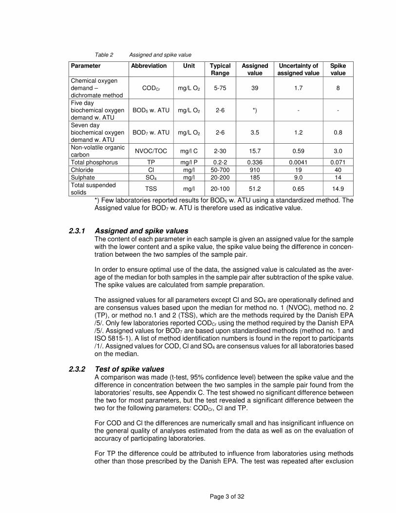
An overview of the concentrations in the samples (the assigned values) and the differ-ence in concentration between the two samples of a sample pair (spike value) are shown in Table 2 compared to the range of concentrations normally encountered in effluent. The table also gives the expanded uncertainty of the assigned values.
Page 3 of 32
Table 2 Assigned and spike value
Parameter Abbreviation Unit Typical
Range
Assigned
value
Uncertainty of
assigned value
Spike
value
Chemical oxygen demand – dichromate method
CODCr mg/L O2 5-75 39 1.7 8
Five day biochemical oxygen demand w. ATU
BOD5 w. ATU mg/L O2 2-6 *) - -
Seven day biochemical oxygen demand w. ATU
BOD7 w. ATU mg/L O2 2-6 3.5 1.2 0.8
Non-volatile organic carbon
NVOC/TOC mg/l C 2-30 15.7 0.59 3.0
Total phosphorus TP mg/l P 0.2-2 0.336 0.0041 0.071 Chloride Cl mg/l 50-700 910 19 40 Sulphate SO4 mg/l 20-200 185 9.0 14 Total suspended solids
TSS mg/l 20-100 51.2 0.65 14.9
*) Few laboratories reported results for BOD5 w. ATU using a standardized method. The Assigned value for BOD7 w. ATU is therefore used as indicative value.
2.3.1 Assigned and spike values The content of each parameter in each sample is given an assigned value for the sample with the lower content and a spike value, the spike value being the difference in concen-tration between the two samples of the sample pair.
In order to ensure optimal use of the data, the assigned value is calculated as the aver-age of the median for both samples in the sample pair after subtraction of the spike value. The spike values are calculated from sample preparation.
The assigned values for all parameters except Cl and SO4 are operationally defined and are consensus values based upon the median for method no. 1 (NVOC), method no. 2 (TP), or method no.1 and 2 (TSS), which are the methods required by the Danish EPA /5/. Only few laboratories reported CODCr using the method required by the Danish EPA /5/. Assigned values for BOD7 are based upon standardised methods (method no. 1 and ISO 5815-1). A list of method identification numbers is found in the report to participants /1/. Assigned values for COD, Cl and SO4 are consensus values for all laboratories based on the median.
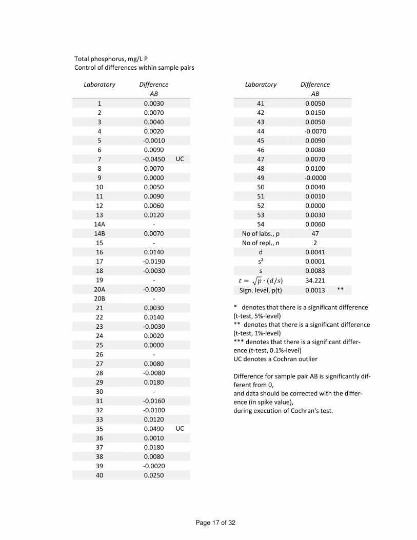
2.3.2 Test of spike values A comparison was made (t-test, 95% confidence level) between the spike value and the difference in concentration between the two samples in the sample pair found from the laboratories’ results, see Appendix C. The test showed no significant difference between the two for most parameters, but the test revealed a significant difference between the two for the following parameters: CODCr, Cl and TP.
For COD and Cl the differences are numerically small and has insignificant influence on the general quality of analyses estimated from the data as well as on the evaluation of accuracy of participating laboratories.
For TP the difference could be attributed to influence from laboratories using methods other than those prescribed by the Danish EPA. The test was repeated after exclusion
Page 4 of 32
of the results for method no. 9, 42, 42A, 42B and 71 and now showed no significant difference.
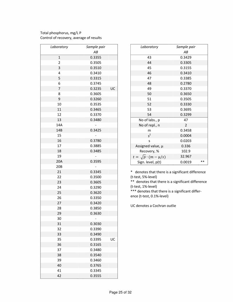
2.3.3 Test of assigned values The assigned value and the average of the results obtained from all laboratories were also compared (t-test, 95% confidence level), see Appendix D. The test showed for most parameters no significant difference between the two and the control of assigned value at Eurofins confirmed the value (Appendix E).
The test revealed a significant difference between the two for TP. Average recovery was 102.9 %. The difference could be attributed to influence from laboratories using methods other than those prescribed by the Danish EPA. The test was repeated after exclusion of the results for method no. 9, 42, 42A, 42B and 71 and now showed no significant difference. Furthermore, the results of control measurements at Eurofins confirmed the assigned value (Appendix E). The assigned value is therefore kept unchanged.
Page 5 of 32
3 HOMOGENEITY AND STABILITY OF SAMPLES
The homogeneity and stability of samples were tested using the following parameters as indicators:
CODCr Combined homogeneity and stability test
TP Combined homogeneity and stability test
TSS Combined homogeneity and stability test
The results of control measurements are shown in Appendix F. The appendix also gives the results of the statistical evaluation of the control data. The data are analysed by analysis of variance (ANOVA) giving:
1. the standard deviation/variance for replicates (the contribution from analytical varia-bility),
2. the between bottle standard deviation/variance (the contribution from heterogeneity) and
3. the between days concentration difference (the contribution from instability).
Homogeneity is evaluated by comparing the between bottle variance to 0.3 * the stand-ard deviation for evaluation of participants’ performance (0.3 ∙ σ�) specified by the Danish EPA /5/, whereas the stability is evaluated by comparing the concentration change of the samples to 0.3 ∙ σ�. This test ensures that heterogeneity and instability will not have neg-ative influence on the evaluation of participant performance /6/.
The appendix also shows the standard deviation within and between laboratories from the proficiency test to allow comparison between tests performed and average quality from participating laboratories.
The tests for stability and homogeneity show that the samples are stable and homoge-neous. However, the test for TP indicated instability. The standard deviation between days (sb) for the method used in the test was taken into account and the difference be-tween /x-y/ and (0.3 ∙ σ�) is found to be marginal.
Page 6 of 32
4 CONCLUSION
The quality control performed, including test of sample stability and homogeneity as well as test of recovery of spike and assigned values, shows that the samples and their as-signed values are suitable for testing the proficiency of the participating laboratories for all parameters. The results are also suitable for estimation of the general quality of anal-yses among all participating laboratories.
For CODCr and Cl the participants could not recover the spike value. The difference be-tween the calculated spike value and that found by the participants is small and the in-fluence on evaluation of participant performance or estimation of general quality of anal-yses is insignificant.
For TP the participants did not recover the spike value or the assigned value. Eurofins’ scrutiny of the combined evidence gave the conclusion that the assigned value is correct. The assigned value is therefore kept unchanged and it is recommended as the basis for evaluation of participating laboratories.
The value given for BOD5 w. ATU is only indicative because the number of participants reporting a results is small. The assigned value is therefore uncertain.
Page 7 of 32
5 REFERENCES
/1/ Eurofins A/S, Proficiency test SPIL-1 (2021), Report to participants, April 2021.
/2/ ISO 5725-2, Accuracy (trueness and precision) of measurement methods and re-sults – Part 2: Basic method for the determination of repeatability and reproducibil-ity of a standard measurement method, 2019.
/3/ Spliid, H., Procedure and analysis of data for proficiency tests and environmental analyses, Report to Danish Environmental Protection Agency, 1994 (in Danish).
/4/ Eurofins A/S, Schedule for a proficiency test, document may be downloaded from www.eurofins.dk/proficiencytest.
/5/ Ministry of Environment regulation no. 1770 on quality criteria for environmental measurements, 28 October 2020 (in Danish).
/6/ ISO 13528, Statistical methods for use in proficiency testing by interlaboratory comparison, 2015.
8
A N N E X E S
Page 9 of 32
ANNEX A LIST OF PARTICIPANTS
Laboratory Town Country
AquaDjurs A/S Grenaa Denmark Biofos A/S København K Denmark Bjergmarken RA, Fors Spildevand Roskilde Roskilde Denmark BlueKolding A/S Kolding Denmark Bornholms Spildevand A/S Rønne Denmark CP Kelco, QC Analyselab. Ll. Skensved Denmark Eurofins Miljø A/S Vejen Denmark Hillerød Spildevand Hillerød Denmark Holbæk RA, Fors Spildevand Holbæk Holbæk Denmark Holstebro Renseanlæg, Vestforsyning Spildevand Holstebro Denmark Kerteminde Forsyning - Spildevand A/S Kerteminde Denmark Klarforsyning, Køge-Egnens Renseanlæg Køge Denmark NK-Forsyning A/S Næstved Denmark Nyborg Forsyning & Service Nyborg Denmark Provas - Haderslev Forsyningsservice A/S Haderslev Denmark Rensningsanlæg Øst, Spildevandslaboratoriet Esbjerg Denmark RGS Nordic A/S Skælskør Denmark Ringkøbing-Skjern Forsyning A/S Skjern Denmark Svendborg Spildevand A/S, Svenborg Centralrenseanlæg
Skårup Fyn Denmark
Vandmiljø Randers A/S Randers SØ Denmark Vejle Spildevand Vejle Denmark Eurofins Umwelt West GmbH Wesseling Germany SYNLAB Analytics AS Norway (Hamar) Hamar Norway AB Borlänge Energi, Borlänge Reningsverk Borlänge Sweden AB Lennart Månsson International Helsingborg Sweden Arctic Paper Munkedals AB Munkedal Sweden Ernemar Laboratorium Oskarshamn Sweden Fiskeby Board AB Norrköping Sweden GRYAAB AB Göteborg Sweden Hallsta Pappersbruk Hallstavik Sweden Hammargårds ARV, Kungsbacka kommun (2 participants)
Kungsbacka Sweden
Holmen Paper AB, Bravikens Pappersbruk Norrköping Sweden INOVYN Sverige AB Stenungsund Sweden Kalmar Vatten AB, VA-lab Kalmar Sweden Klippans Reningsverk Klippan Sweden Kristianstad Kommun Kristianstad Sweden Käppalaverket Lidingö Sweden Laboratoriet Fillanverket, MittSverige Vatten och Av-fall AB
Sundsvall Sweden
Laboratoriet vid Smedjeholms avloppsreningsverk Falkenberg Sweden Ljungby Kommun, Avloppsreningsverket, VA-labb Ljungby Sweden Mjölby Kommun Mjölby Sweden
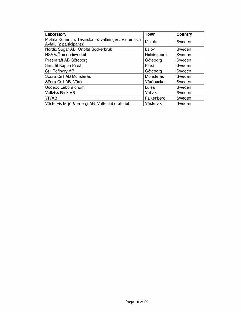
Page 10 of 32
Laboratory Town Country
Motala Kommun, Tekniska Förvaltningen, Vatten och Avfall, (2 participants)
Motala Sweden
Nordic Sugar AB, Örtofta Sockerbruk Eslöv Sweden NSVA/Öresundsverket Helsingborg Sweden Preemraff AB Göteborg Göteborg Sweden Smurfit Kappa Piteå Piteå Sweden St1 Refinery AB Göteborg Sweden Södra Cell AB Mönsterås Mönsterås Sweden Södra Cell AB, Värö Väröbacka Sweden Uddebo Laboratorium Luleå Sweden Vallviks Bruk AB Vallvik Sweden VIVAB Falkenberg Sweden Västervik Miljö & Energi AB, Vattenlaboratoriet Västervik Sweden
Page 11 of 32
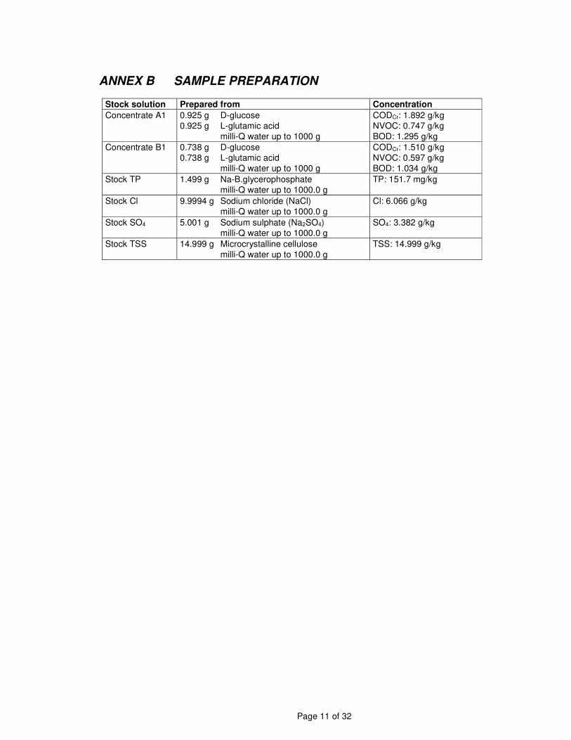
ANNEX B SAMPLE PREPARATION
Stock solution Prepared from Concentration
Concentrate A1 0.925 g D-glucose 0.925 g L-glutamic acid milli-Q water up to 1000 g
CODCr: 1.892 g/kg NVOC: 0.747 g/kg BOD: 1.295 g/kg
Concentrate B1 0.738 g D-glucose 0.738 g L-glutamic acid milli-Q water up to 1000 g
CODCr: 1.510 g/kg NVOC: 0.597 g/kg BOD: 1.034 g/kg
Stock TP 1.499 g Na-B.glycerophosphate milli-Q water up to 1000.0 g
TP: 151.7 mg/kg
Stock Cl 9.9994 g Sodium chloride (NaCl) milli-Q water up to 1000.0 g
Cl: 6.066 g/kg
Stock SO4 5.001 g Sodium sulphate (Na2SO4) milli-Q water up to 1000.0 g
SO4: 3.382 g/kg
Stock TSS 14.999 g Microcrystalline cellulose milli-Q water up to 1000.0 g
TSS: 14.999 g/kg
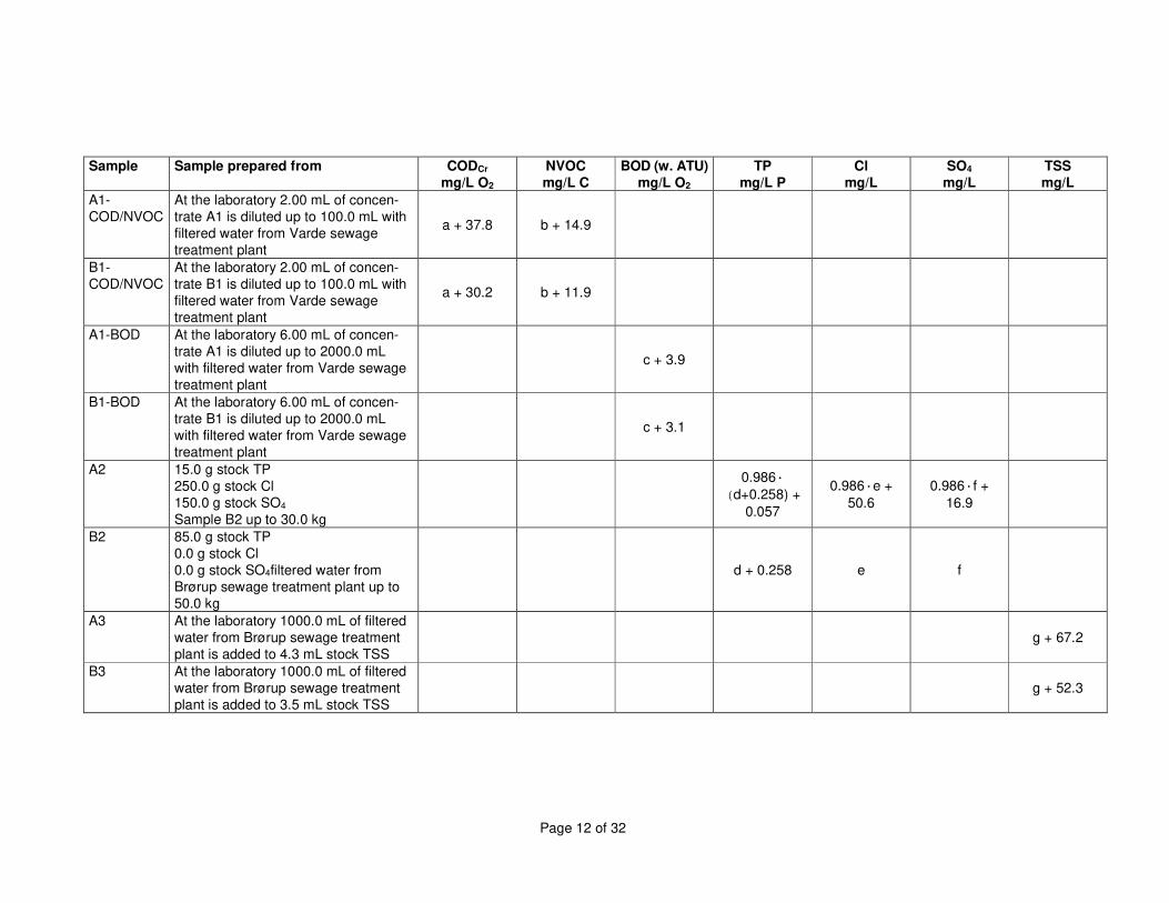
Page 12 of 32
Sample Sample prepared from CODCr
mg/L O2
NVOC
mg/L C
BOD (w. ATU)
mg/L O2
TP
mg/L P
Cl
mg/L
SO4
mg/L
TSS
mg/L
A1-COD/NVOC
At the laboratory 2.00 mL of concen-trate A1 is diluted up to 100.0 mL with filtered water from Varde sewage treatment plant
a + 37.8 b + 14.9
B1-COD/NVOC
At the laboratory 2.00 mL of concen-trate B1 is diluted up to 100.0 mL with filtered water from Varde sewage treatment plant
a + 30.2 b + 11.9
A1-BOD At the laboratory 6.00 mL of concen-trate A1 is diluted up to 2000.0 mL with filtered water from Varde sewage treatment plant
c + 3.9
B1-BOD At the laboratory 6.00 mL of concen-trate B1 is diluted up to 2000.0 mL with filtered water from Varde sewage treatment plant
c + 3.1
A2 15.0 g stock TP 250.0 g stock Cl 150.0 g stock SO4 Sample B2 up to 30.0 kg
0.986·(d+0.258) +
0.057
0.986·e + 50.6
0.986·f + 16.9
B2 85.0 g stock TP 0.0 g stock Cl 0.0 g stock SO4filtered water from Brørup sewage treatment plant up to 50.0 kg
d + 0.258 e f
A3 At the laboratory 1000.0 mL of filtered water from Brørup sewage treatment plant is added to 4.3 mL stock TSS
g + 67.2
B3 At the laboratory 1000.0 mL of filtered water from Brørup sewage treatment plant is added to 3.5 mL stock TSS
g + 52.3
Page 13 of 32
ANNEX C CONTROL OF SPIKE VALUES
CODCr, mg/L O2
Control of differences within sample pairs
Laboratory Difference
AB
1 -
2 -0.40
3 -2.10
4 1.10
5 -
6 -5.00
7 -
8 -3.60
9 -3.60
10 -0.50
11 -
12 -0.90
13 -1.40
14A -
14B 2.00
15 6.60
16 1.46
17 -3.00
18 -2.30
19 -
20A -1.90
20B -2.00
21 2.70
22 -
23 -0.70
24 -
25 -1.10
26 -17.70 UC
27 0.40
28 -0.50
29 -1.60
30 0.70
31 -
32 -
33 0.60
35 -0.60
36 -
37 -2.50
38 -
Laboratory Difference
AB
39 -
40 -
41 -2.90
42 -2.10
43 -5.05
44 -1.60
45 -
46 -6.70
47 0.50
48 -3.00
49 -
50 9.00
51 -2.80
52 -
53 -2.10
54 -3.70
No of labs., p 37
No of repl., n 2
d -1.04
s² 8.68
s 2.95
� = ∙ (�/�) -21.535
Sign. level, p(t) 0.0381 *
* denotes that there is a significant difference
(t-test, 5%-level)
** denotes that there is a significant difference
(t-test, 1%-level)
*** denotes that there is a significant differ-
ence (t-test, 0.1%-level)
UC denotes a Cochran outlier
Difference for sample pair AB is significantly
different from 0,
and data should be corrected with the differ-
ence (in spike value),
during execution of Cochran's test.
Page 14 of 32
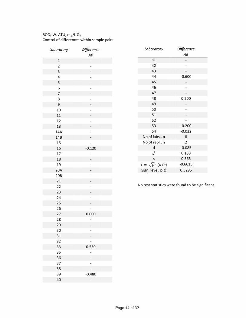
BOD5 W. ATU, mg/L O2
Control of differences within sample pairs
Laboratory Difference
AB
1 -
2 -
3 -
4 -
5 -
6 -
7 -
8 -
9 -
10 -
11 -
12 -
13 -
14A -
14B -
15 -
16 -0.120
17 -
18 -
19 -
20A -
20B -
21 -
22 -
23 -
24 -
25 -
26 -
27 0.000
28 -
29 -
30 -
31 -
32 -
33 0.550
35 -
36 -
37 -
38 -
39 -0.480
40 -
Laboratory Difference
AB
41 -
42 -
43 -
44 -0.600
45 -
46 -
47 -
48 0.200
49 -
50 -
51 -
52 -
53 -0.200
54 -0.032
No of labs., p 8
No of repl., n 2
d -0.085
s2 0.133
s 0.365
� = ∙ (�/�) -0.6615
Sign. level, p(t) 0.5295
No test statistics were found to be significant
Page 15 of 32
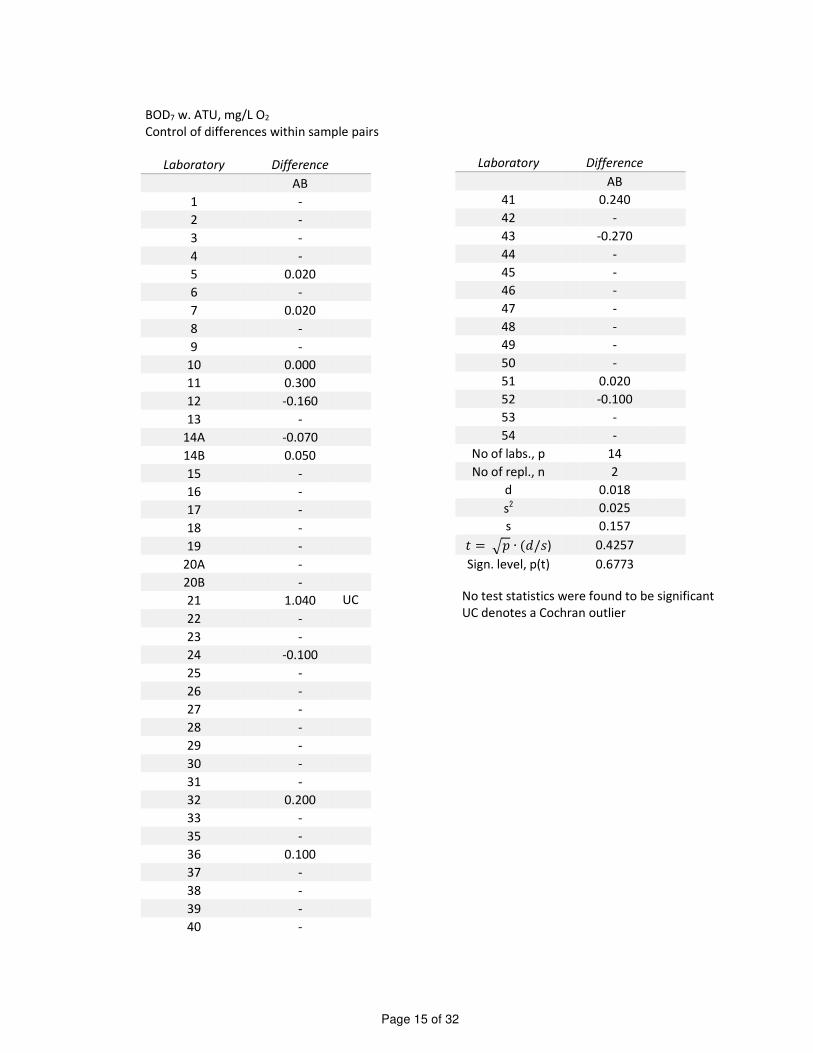
BOD7 w. ATU, mg/L O2
Control of differences within sample pairs
Laboratory Difference
AB
1 -
2 -
3 -
4 -
5 0.020
6 -
7 0.020
8 -
9 -
10 0.000
11 0.300
12 -0.160
13 -
14A -0.070
14B 0.050
15 -
16 -
17 -
18 -
19 -
20A -
20B -
21 1.040 UC
22 -
23 -
24 -0.100
25 -
26 -
27 -
28 -
29 -
30 -
31 -
32 0.200
33 -
35 -
36 0.100
37 -
38 -
39 -
40 -
Laboratory Difference
AB
41 0.240
42 -
43 -0.270
44 -
45 -
46 -
47 -
48 -
49 -
50 -
51 0.020
52 -0.100
53 -
54 -
No of labs., p 14
No of repl., n 2
d 0.018
s2 0.025
s 0.157
� = ∙ (�/�) 0.4257
Sign. level, p(t) 0.6773
No test statistics were found to be significant
UC denotes a Cochran outlier
Page 16 of 32
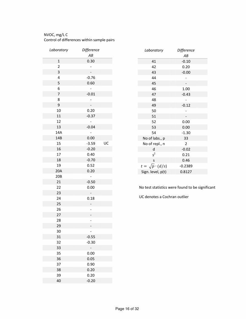
NVOC, mg/L C
Control of differences within sample pairs
Laboratory Difference
AB
1 0.30
2 -
3 -
4 -0.76
5 0.60
6 -
7 -0.01
8 -
9 -
10 0.20
11 -0.37
12 -
13 -0.04
14A -
14B 0.00
15 -3.59 UC
16 -0.20
17 0.40
18 -0.70
19 0.52
20A 0.20
20B -
21 -0.50
22 0.00
23 -
24 0.18
25 -
26 -
27 -
28 -
29 -
30 -
31 -0.55
32 -0.30
33 -
35 0.00
36 0.05
37 0.90
38 0.20
39 0.20
40 -0.20
Laboratory Difference
AB
41 -0.10
42 0.20
43 -0.00
44 -
45 -
46 1.00
47 -0.43
48 -
49 -0.12
50 -
51 -
52 0.00
53 0.00
54 -1.30
No of labs., p 33
No of repl., n 2
d -0.02
s2 0.21
s 0.46
� = ∙ (�/�) -0.2389
Sign. level, p(t) 0.8127
No test statistics were found to be significant
UC denotes a Cochran outlier
Page 17 of 32
Total phosphorus, mg/L P
Control of differences within sample pairs
Laboratory Difference
AB
1 0.0030
2 0.0070
3 0.0040
4 0.0020
5 -0.0010
6 0.0090
7 -0.0450 UC
8 0.0070
9 0.0000
10 0.0050
11 0.0090
12 0.0060
13 0.0120
14A -
14B 0.0070
15 -
16 0.0140
17 -0.0190
18 -0.0030
19 -
20A -0.0030
20B -
21 0.0030
22 0.0140
23 -0.0030
24 0.0020
25 0.0000
26 -
27 0.0080
28 -0.0080
29 0.0180
30 -
31 -0.0160
32 -0.0100
33 0.0120
35 0.0490 UC
36 0.0010
37 0.0180
38 0.0080
39 -0.0020
40 0.0250
Laboratory Difference
AB
41 0.0050
42 0.0150
43 0.0050
44 -0.0070
45 0.0090
46 0.0080
47 0.0070
48 0.0100
49 -0.0000
50 0.0040
51 0.0010
52 0.0000
53 0.0030
54 0.0060
No of labs., p 47
No of repl., n 2
d 0.0041
s² 0.0001
s 0.0083
� = ∙ (�/�) 34.221
Sign. level, p(t) 0.0013 **
* denotes that there is a significant difference
(t-test, 5%-level)
** denotes that there is a significant difference
(t-test, 1%-level)
*** denotes that there is a significant differ-
ence (t-test, 0.1%-level)
UC denotes a Cochran outlier
Difference for sample pair AB is significantly dif-
ferent from 0,
and data should be corrected with the differ-
ence (in spike value),
during execution of Cochran's test.
Page 18 of 32
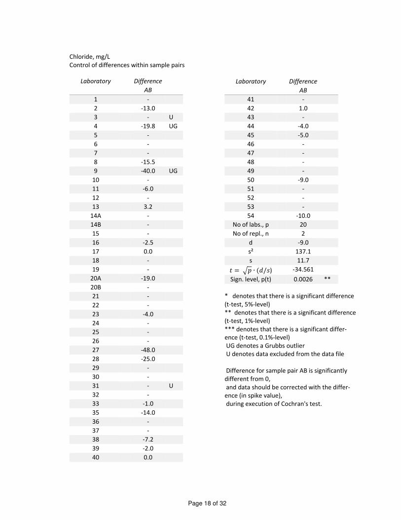
Chloride, mg/L
Control of differences within sample pairs
Laboratory Difference
AB
1 -
2 -13.0
3 - U
4 -19.8 UG
5 -
6 -
7 -
8 -15.5
9 -40.0 UG
10 -
11 -6.0
12 -
13 3.2
14A -
14B -
15 -
16 -2.5
17 0.0
18 -
19 -
20A -19.0
20B -
21 -
22 -
23 -4.0
24 -
25 -
26 -
27 -48.0
28 -25.0
29 -
30 -
31 - U
32 -
33 -1.0
35 -14.0
36 -
37 -
38 -7.2
39 -2.0
40 0.0
Laboratory Difference
AB
41 -
42 1.0
43 -
44 -4.0
45 -5.0
46 -
47 -
48 -
49 -
50 -9.0
51 -
52 -
53 -
54 -10.0
No of labs., p 20
No of repl., n 2
d -9.0
s² 137.1
s 11.7
� = ∙ (�/�) -34.561
Sign. level, p(t) 0.0026 **
* denotes that there is a significant difference
(t-test, 5%-level)
** denotes that there is a significant difference
(t-test, 1%-level)
*** denotes that there is a significant differ-
ence (t-test, 0.1%-level)
UG denotes a Grubbs outlier
U denotes data excluded from the data file
Difference for sample pair AB is significantly
different from 0,
and data should be corrected with the differ-
ence (in spike value),
during execution of Cochran's test.
Page 19 of 32
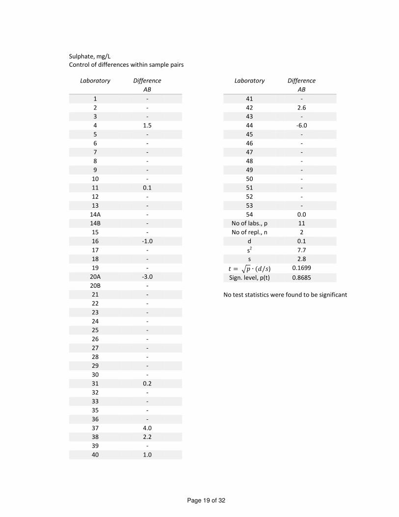
Sulphate, mg/L
Control of differences within sample pairs
Laboratory Difference
AB
1 -
2 -
3 -
4 1.5
5 -
6 -
7 -
8 -
9 -
10 -
11 0.1
12 -
13 -
14A -
14B -
15 -
16 -1.0
17 -
18 -
19 -
20A -3.0
20B -
21 -
22 -
23 -
24 -
25 -
26 -
27 -
28 -
29 -
30 -
31 0.2
32 -
33 -
35 -
36 -
37 4.0
38 2.2
39 -
40 1.0
Laboratory Difference
AB
41 -
42 2.6
43 -
44 -6.0
45 -
46 -
47 -
48 -
49 -
50 -
51 -
52 -
53 -
54 0.0
No of labs., p 11
No of repl., n 2
d 0.1
s2 7.7
s 2.8
� = ∙ (�/�) 0.1699
Sign. level, p(t) 0.8685
No test statistics were found to be significant
Page 20 of 32
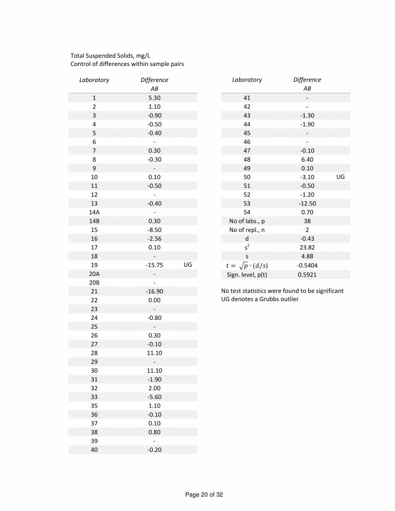
Total Suspended Solids, mg/L
Control of differences within sample pairs
Laboratory Difference
AB
1 5.30
2 1.10
3 -0.90
4 -0.50
5 -0.40
6 -
7 0.30
8 -0.30
9 -
10 0.10
11 -0.50
12 -
13 -0.40
14A -
14B 0.30
15 -8.50
16 -2.56
17 0.10
18 -
19 -15.75 UG
20A -
20B -
21 -16.90
22 0.00
23 -
24 -0.80
25 -
26 0.30
27 -0.10
28 11.10
29 -
30 11.10
31 -1.90
32 2.00
33 -5.60
35 1.10
36 -0.10
37 0.10
38 0.80
39 -
40 -0.20
Laboratory Difference
AB
41 -
42 -
43 -1.30
44 -1.90
45 -
46 -
47 -0.10
48 6.40
49 0.10
50 -3.10 UG
51 -0.50
52 -1.20
53 -12.50
54 0.70
No of labs., p 38
No of repl., n 2
d -0.43
s2 23.82
s 4.88
� = ∙ (�/�) -0.5404
Sign. level, p(t) 0.5921
No test statistics were found to be significant
UG denotes a Grubbs outlier
Page 21 of 32
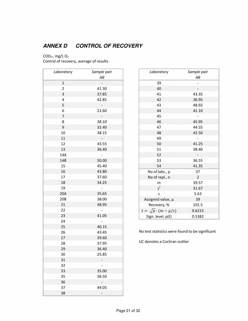
ANNEX D CONTROL OF RECOVERY
CODCr, mg/L O2
Control of recovery, average of results
Laboratory Sample pair
AB
1 -
2 41.30
3 37.85
4 42.85
5 -
6 22.60
7 -
8 38.10
9 32.40
10 38.15
11 -
12 43.55
13 36.40
14A -
14B 50.00
15 45.40
16 43.80
17 37.60
18 34.25
19 -
20A 35.65
20B 38.00
21 48.95
22 -
23 41.05
24 -
25 40.15
26 43.45
27 39.60
28 37.95
29 36.40
30 25.85
31 -
32 -
33 35.00
35 36.50
36 -
37 44.05
38 -
Laboratory Sample pair
AB
39 -
40 -
41 43.35
42 36.95
43 48.92
44 41.10
45 -
46 45.95
47 44.55
48 42.50
49 -
50 41.25
51 38.40
52 -
53 36.55
54 41.35
No of labs., p 37
No of repl., n 2
m 39.57
s2 31.67
s 5.63
Assigned value, µ 39
Recovery, % 101.5
� = ∙ (� − µ/�) 0.6215
Sign. level, p(t) 0.5382
No test statistics were found to be significant
UC denotes a Cochran outlier
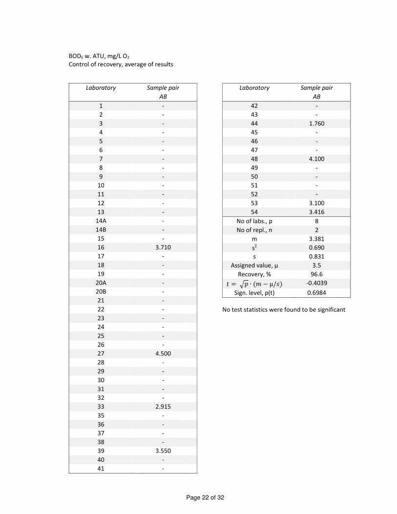
Page 22 of 32
BOD5 w. ATU, mg/L O2
Control of recovery, average of results
Laboratory Sample pair
AB
1 -
2 -
3 -
4 -
5 -
6 -
7 -
8 -
9 -
10 -
11 -
12 -
13 -
14A -
14B -
15 -
16 3.710
17 -
18 -
19 -
20A -
20B -
21 -
22 -
23 -
24 -
25 -
26 -
27 4.500
28 -
29 -
30 -
31 -
32 -
33 2.915
35 -
36 -
37 -
38 -
39 3.550
40 -
41 -
Laboratory Sample pair
AB
42 -
43 -
44 1.760
45 -
46 -
47 -
48 4.100
49 -
50 -
51 -
52 -
53 3.100
54 3.416
No of labs., p 8
No of repl., n 2
m 3.381
s2 0.690
s 0.831
Assigned value, µ 3.5
Recovery, % 96.6
� = ∙ (� − µ/�) -0.4039
Sign. level, p(t) 0.6984
No test statistics were found to be significant
Page 23 of 32
BOD7 w. ATU, mg/L O2
Control of recovery, average of results
Laboratory Sample pair
AB
1 -
2 -
3 -
4 -
5 4.820
6 -
7 4.580
8 -
9 -
10 4.100
11 4.550
12 4.990
13 -
14A 4.585
14B 4.525
15 -
16 -
17 -
18 -
19 -
20A -
20B -
21 3.850 UC
22 -
23 -
24 4.350
25 -
26 -
27 -
28 -
29 -
30 -
31 -
32 5.000
33 -
35 -
36 4.280
37 -
38 -
39 -
40 -
41 4.690
42 -
Laboratory Sample pair
AB
43 4.255
44 -
45 -
46 -
47 -
48 -
49 -
50 -
51 4.340
52 4.850
53 -
54 -
No of labs., p 14
No of repl., n 2
m 4.565
s2 0.079
s 0.281
Assigned value, µ 4.5
Recovery, % 101.5
� = ∙ (� − µ/�) 0.8711
Sign. level, p(t) 0.3995
No test statistics were found to be significant
UC denotes a Cochran outlier
Page 24 of 32
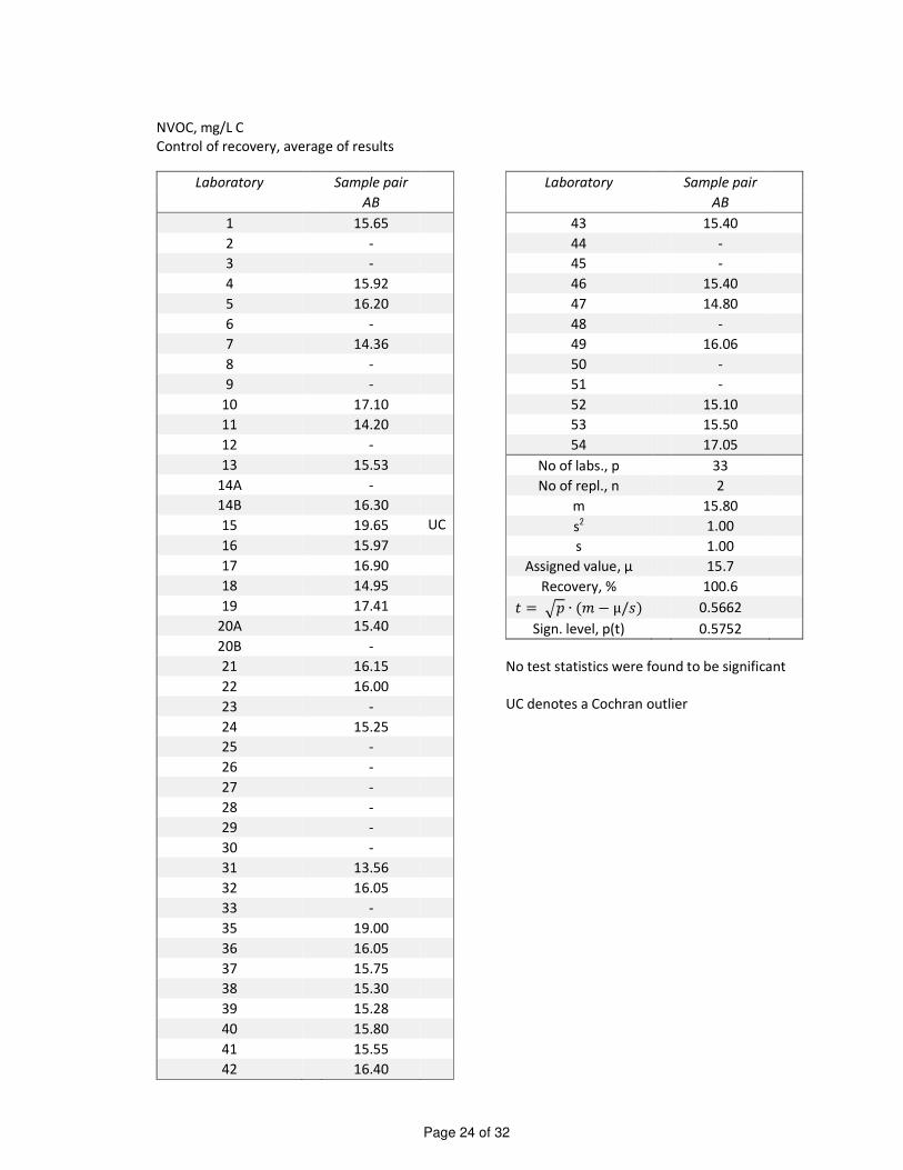
NVOC, mg/L C
Control of recovery, average of results
Laboratory Sample pair
AB
1 15.65
2 -
3 -
4 15.92
5 16.20
6 -
7 14.36
8 -
9 -
10 17.10
11 14.20
12 -
13 15.53
14A -
14B 16.30
15 19.65 UC
16 15.97
17 16.90
18 14.95
19 17.41
20A 15.40
20B -
21 16.15
22 16.00
23 -
24 15.25
25 -
26 -
27 -
28 -
29 -
30 -
31 13.56
32 16.05
33 -
35 19.00
36 16.05
37 15.75
38 15.30
39 15.28
40 15.80
41 15.55
42 16.40
Laboratory Sample pair
AB
43 15.40
44 -
45 -
46 15.40
47 14.80
48 -
49 16.06
50 -
51 -
52 15.10
53 15.50
54 17.05
No of labs., p 33
No of repl., n 2
m 15.80
s2 1.00
s 1.00
Assigned value, µ 15.7
Recovery, % 100.6
� = ∙ (� − µ/�) 0.5662
Sign. level, p(t) 0.5752
No test statistics were found to be significant
UC denotes a Cochran outlier
Page 25 of 32
Total phosphorus, mg/L P
Control of recovery, average of results
Laboratory Sample pair
AB
1 0.3355
2 0.3505
3 0.3510
4 0.3410
5 0.3315
6 0.3745
7 0.3235 UC
8 0.3605
9 0.3260
10 0.3535
11 0.3465
12 0.3370
13 0.3480
14A -
14B 0.3425
15 -
16 0.3780
17 0.3885
18 0.3485
19 -
20A 0.3595
20B -
21 0.3345
22 0.3500
23 0.3605
24 0.3290
25 0.3620
26 0.3350
27 0.3420
28 0.3850
29 0.3630
30 -
31 0.3030
32 0.3390
33 0.3490
35 0.3395 UC
36 0.3165
37 0.3480
38 0.3540
39 0.3460
40 0.3765
41 0.3345
42 0.3555
Laboratory Sample pair
AB
43 0.3429
44 0.3305
45 0.3155
46 0.3410
47 0.3385
48 0.2780
49 0.3370
50 0.3650
51 0.3505
52 0.3330
53 0.3695
54 0.3299
No of labs., p 47
No of repl., n 2
m 0.3458
s2 0.0004
s 0.0203
Assigned value, µ 0.336
Recovery, % 102.9
� = ∙ (� − µ/�) 32.967
Sign. level, p(t) 0.0019 **
* denotes that there is a significant difference
(t-test, 5%-level)
** denotes that there is a significant difference
(t-test, 1%-level)
*** denotes that there is a significant differ-
ence (t-test, 0.1%-level)
UC denotes a Cochran outlie
Page 26 of 32
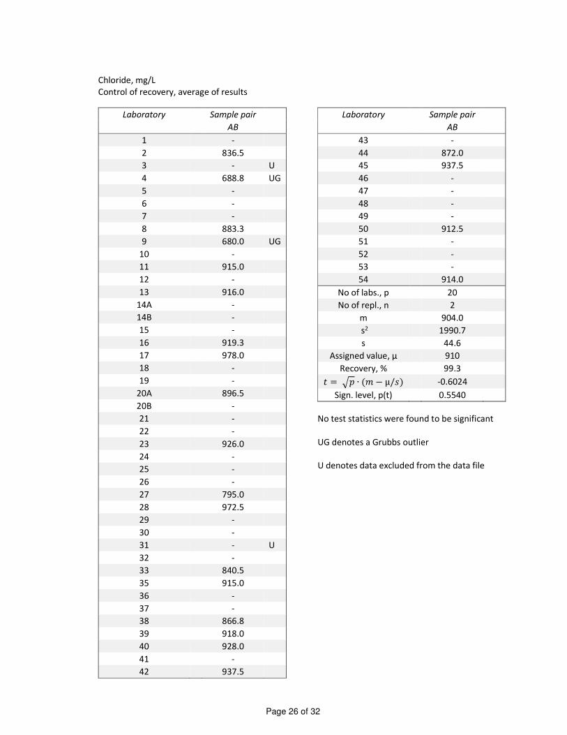
Chloride, mg/L
Control of recovery, average of results
Laboratory Sample pair
AB
1 -
2 836.5
3 - U
4 688.8 UG
5 -
6 -
7 -
8 883.3
9 680.0 UG
10 -
11 915.0
12 -
13 916.0
14A -
14B -
15 -
16 919.3
17 978.0
18 -
19 -
20A 896.5
20B -
21 -
22 -
23 926.0
24 -
25 -
26 -
27 795.0
28 972.5
29 -
30 -
31 - U
32 -
33 840.5
35 915.0
36 -
37 -
38 866.8
39 918.0
40 928.0
41 -
42 937.5
Laboratory Sample pair
AB
43 -
44 872.0
45 937.5
46 -
47 -
48 -
49 -
50 912.5
51 -
52 -
53 -
54 914.0
No of labs., p 20
No of repl., n 2
m 904.0
s2 1990.7
s 44.6
Assigned value, µ 910
Recovery, % 99.3
� = ∙ (� − µ/�) -0.6024
Sign. level, p(t) 0.5540
No test statistics were found to be significant
UG denotes a Grubbs outlier
U denotes data excluded from the data file
Page 27 of 32
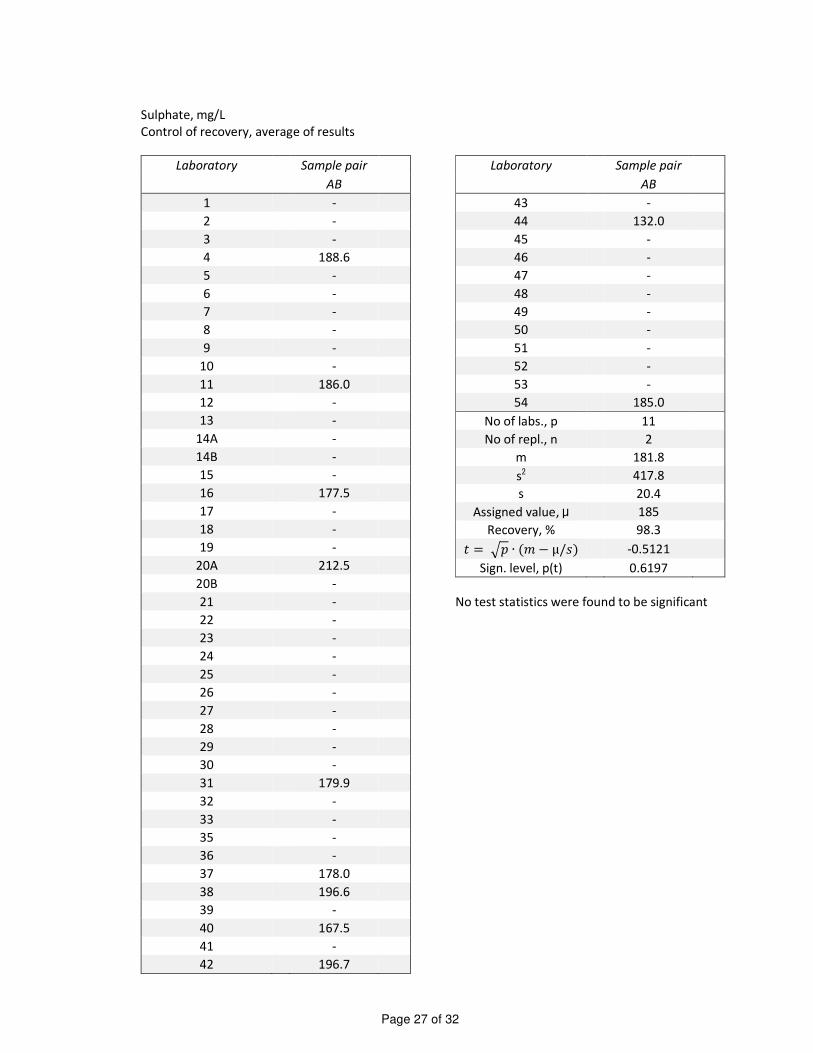
Sulphate, mg/L
Control of recovery, average of results
Laboratory Sample pair
AB
1 -
2 -
3 -
4 188.6
5 -
6 -
7 -
8 -
9 -
10 -
11 186.0
12 -
13 -
14A -
14B -
15 -
16 177.5
17 -
18 -
19 -
20A 212.5
20B -
21 -
22 -
23 -
24 -
25 -
26 -
27 -
28 -
29 -
30 -
31 179.9
32 -
33 -
35 -
36 -
37 178.0
38 196.6
39 -
40 167.5
41 -
42 196.7
Laboratory Sample pair
AB
43 -
44 132.0
45 -
46 -
47 -
48 -
49 -
50 -
51 -
52 -
53 -
54 185.0
No of labs., p 11
No of repl., n 2
m 181.8
s2 417.8
s 20.4
Assigned value, µ 185
Recovery, % 98.3
� = ∙ (� − µ/�) -0.5121
Sign. level, p(t) 0.6197
No test statistics were found to be significant
Page 28 of 32
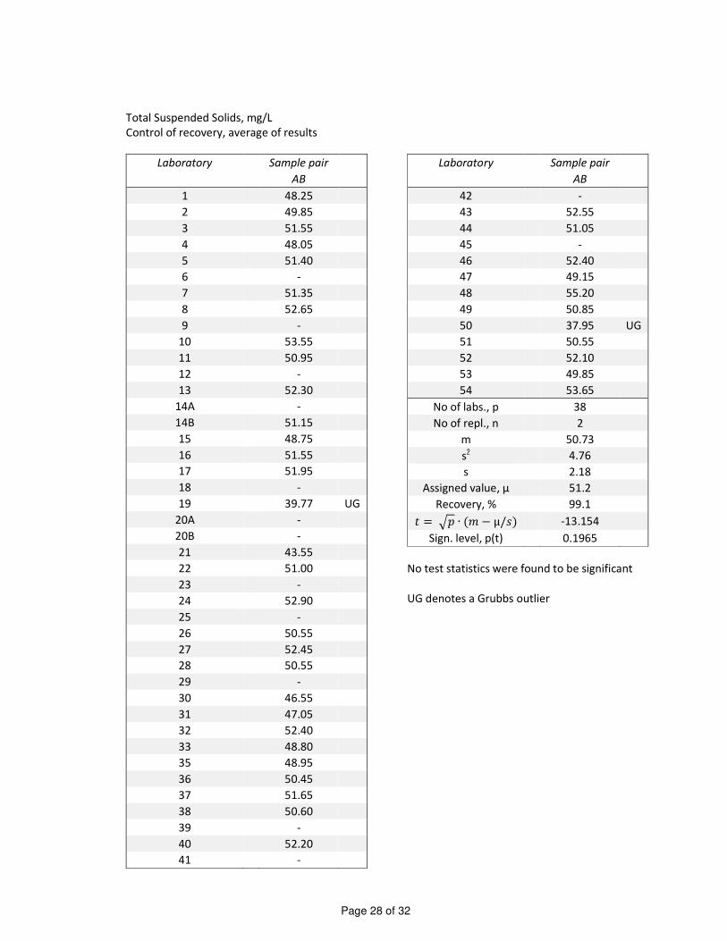
Total Suspended Solids, mg/L
Control of recovery, average of results
Laboratory Sample pair
AB
1 48.25
2 49.85
3 51.55
4 48.05
5 51.40
6 -
7 51.35
8 52.65
9 -
10 53.55
11 50.95
12 -
13 52.30
14A -
14B 51.15
15 48.75
16 51.55
17 51.95
18 -
19 39.77 UG
20A -
20B -
21 43.55
22 51.00
23 -
24 52.90
25 -
26 50.55
27 52.45
28 50.55
29 -
30 46.55
31 47.05
32 52.40
33 48.80
35 48.95
36 50.45
37 51.65
38 50.60
39 -
40 52.20
41 -
Laboratory Sample pair
AB
42 -
43 52.55
44 51.05
45 -
46 52.40
47 49.15
48 55.20
49 50.85
50 37.95 UG
51 50.55
52 52.10
53 49.85
54 53.65
No of labs., p 38
No of repl., n 2
m 50.73
s2 4.76
s 2.18
Assigned value, µ 51.2
Recovery, % 99.1
� = ∙ (� − µ/�) -13.154
Sign. level, p(t) 0.1965
No test statistics were found to be significant
UG denotes a Grubbs outlier
Page 29 of 32
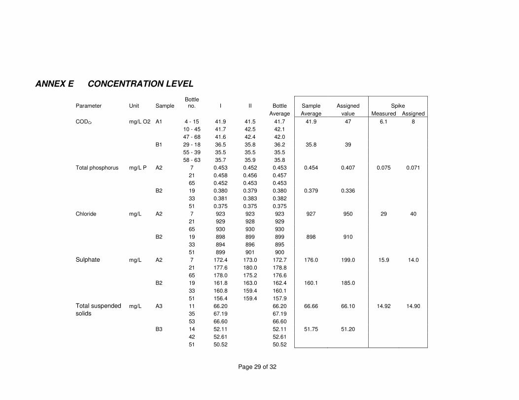
ANNEX E CONCENTRATION LEVEL
Parameter Unit Sample Bottle
no. I II Bottle Sample Assigned Spike Average Average value Measured Assigned
CODCr mg/L O2 A1 4 - 15 41.9 41.5 41.7 41.9 47 6.1 8 10 - 45 41.7 42.5 42.1 47 - 68 41.6 42.4 42.0
B1 29 - 18 36.5 35.8 36.2 35.8 39 55 - 39 35.5 35.5 35.5 58 - 63 35.7 35.9 35.8
Total phosphorus mg/L P A2 7 0.453 0.452 0.453 0.454 0.407 0.075 0.071 21 0.458 0.456 0.457 65 0.452 0.453 0.453
B2 19 0.380 0.379 0.380 0.379 0.336 33 0.381 0.383 0.382 51 0.375 0.375 0.375
Chloride mg/L A2 7 923 923 923 927 950 29 40 21 929 928 929 65 930 930 930
B2 19 898 899 899 898 910 33 894 896 895 51 899 901 900
Sulphate mg/L A2 7 172.4 173.0 172.7 176.0 199.0 15.9 14.0 21 177.6 180.0 178.8 65 178.0 175.2 176.6
B2 19 161.8 163.0 162.4 160.1 185.0 33 160.8 159.4 160.1 51 156.4 159.4 157.9
Total suspended mg/L A3 11 66.20 66.20 66.66 66.10 14.92 14.90 solids 35 67.19 67.19
53 66.60 66.60 B3 14 52.11 52.11 51.75 51.20
42 52.61 52.61 51 50.52 50.52
Page 30 of 32
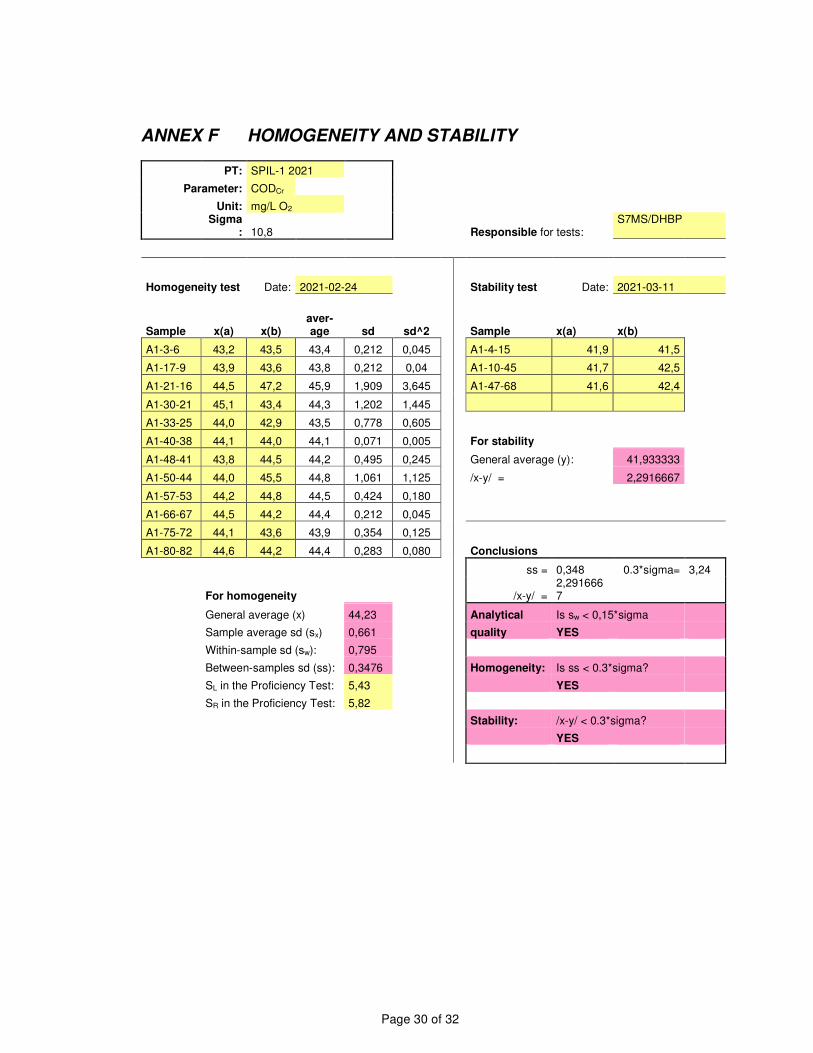
ANNEX F HOMOGENEITY AND STABILITY
PT: SPIL-1 2021
Parameter: CODCr
Unit: mg/L O2
Sigma
: 10,8 Responsible for tests: S7MS/DHBP
Homogeneity test Date: 2021-02-24 Stability test Date: 2021-03-11
Sample x(a) x(b) aver-age sd sd^2 Sample x(a) x(b)
A1-3-6 43,2 43,5 43,4 0,212 0,045 A1-4-15 41,9 41,5 A1-17-9 43,9 43,6 43,8 0,212 0,04 A1-10-45 41,7 42,5 A1-21-16 44,5 47,2 45,9 1,909 3,645 A1-47-68 41,6 42,4 A1-30-21 45,1 43,4 44,3 1,202 1,445 A1-33-25 44,0 42,9 43,5 0,778 0,605
A1-40-38 44,1 44,0 44,1 0,071 0,005 For stability
A1-48-41 43,8 44,5 44,2 0,495 0,245 General average (y): 41,933333 A1-50-44 44,0 45,5 44,8 1,061 1,125 /x-y/ = 2,2916667 A1-57-53 44,2 44,8 44,5 0,424 0,180
A1-66-67 44,5 44,2 44,4 0,212 0,045
A1-75-72 44,1 43,6 43,9 0,354 0,125
A1-80-82 44,6 44,2 44,4 0,283 0,080 Conclusions
ss = 0,348 0.3*sigma= 3,24
For homogeneity /x-y/ = 2,2916667
General average (x) 44,23 Analytical Is sw < 0,15*sigma
Sample average sd (sx) 0,661 quality YES
Within-sample sd (sw): 0,795
Between-samples sd (ss): 0,3476 Homogeneity: Is ss < 0.3*sigma?
SL in the Proficiency Test: 5,43 YES
SR in the Proficiency Test: 5,82
Stability: /x-y/ < 0.3*sigma?
YES
Page 31 of 32
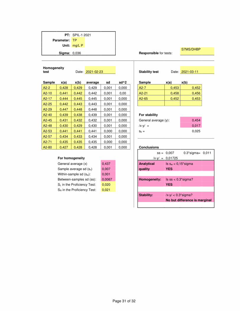
PT: SPIL-1 2021
Parameter: TP
Unit: mg/L P
Sigma: 0,036 Responsible for tests: S7MS/DHBP
Homogeneity test Date: 2021-02-23 Stability test Date: 2021-03-11
Sample x(a) x(b) average sd sd^2 Sample x(a) x(b)
A2-2 0,428 0,429 0,429 0,001 0,000 A2-7 0,453 0,452 A2-10 0,441 0,442 0,442 0,001 0,00 A2-21 0,458 0,456 A2-17 0,444 0,445 0,445 0,001 0,000 A2-65 0,452 0,453 A2-25 0,442 0,443 0,443 0,001 0,000 A2-29 0,447 0,448 0,448 0,001 0,000
A2-40 0,439 0,438 0,439 0,001 0,000 For stability
A2-45 0,431 0,432 0,432 0,001 0,000 General average (y): 0,454 A2-48 0,430 0,429 0,430 0,001 0,000 /x-y/ = 0,017 A2-53 0,441 0,441 0,441 0,000 0,000 sb = 0,025 A2-57 0,434 0,433 0,434 0,001 0,000
A2-71 0,435 0,435 0,435 0,000 0,000
A2-80 0,427 0,428 0,428 0,001 0,000 Conclusions
ss = 0,007 0.3*sigma= 0,011
For homogeneity /x-y/ = 0,01725
General average (x) 0,437 Analytical Is sw < 0,15*sigma
Sample average sd (sx) 0,007 quality YES
Within-sample sd (sw): 0,001
Between-samples sd (ss): 0,0067 Homogeneity: Is ss < 0.3*sigma?
SL in the Proficiency Test: 0,020 YES
SR in the Proficiency Test: 0,021
Stability: /x-y/ < 0.3*sigma?
No but difference is marginal
Page 32 of 32
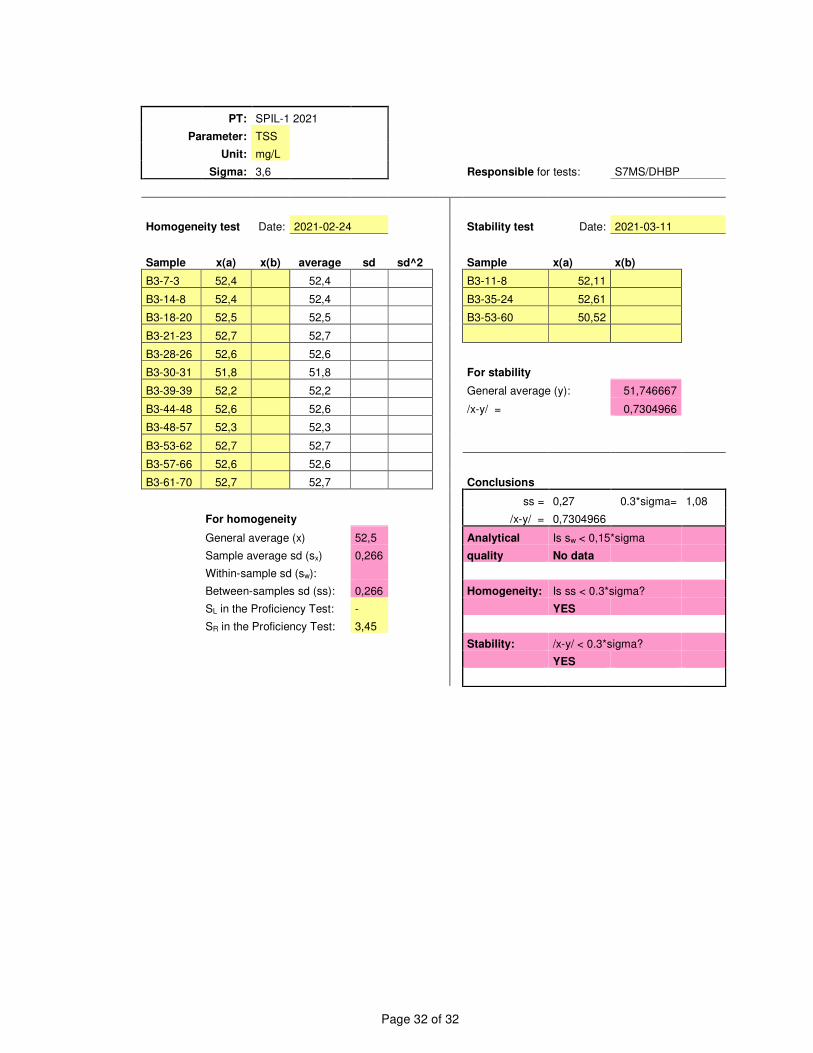
PT: SPIL-1 2021
Parameter: TSS
Unit: mg/L
S7MS/DHBP Sigma: 3,6 Responsible for tests:
Homogeneity test Date: 2021-02-24 Stability test Date: 2021-03-11
Sample x(a) x(b) average sd sd^2 Sample x(a) x(b)
B3-7-3 52,4 52,4 B3-11-8 52,11 B3-14-8 52,4 52,4 B3-35-24 52,61 B3-18-20 52,5 52,5 B3-53-60 50,52 B3-21-23 52,7 52,7 B3-28-26 52,6 52,6
B3-30-31 51,8 51,8 For stability
B3-39-39 52,2 52,2 General average (y): 51,746667 B3-44-48 52,6 52,6 /x-y/ = 0,7304966 B3-48-57 52,3 52,3
B3-53-62 52,7 52,7
B3-57-66 52,6 52,6
B3-61-70 52,7 52,7 Conclusions
ss = 0,27 0.3*sigma= 1,08
For homogeneity /x-y/ = 0,7304966
General average (x) 52,5 Analytical Is sw < 0,15*sigma
Sample average sd (sx) 0,266 quality No data
Within-sample sd (sw):
Between-samples sd (ss): 0,266 Homogeneity: Is ss < 0.3*sigma?
SL in the Proficiency Test: - YES
SR in the Proficiency Test: 3,45
Stability: /x-y/ < 0.3*sigma?
YES