uncertainty analysis in rock mass - colorado school of mines
TRANSCRIPT
ii
UNCERTAINTY ANALYSIS IN ROCK MASS CLASSIFICATION AND ITS APPLICATION TO RELIABILITY
EVALUATION IN TUNNEL CONSTRUCTION
FINAL PROJECT REPORT
by Dr. Hui Lu1
Dr. Marte Gutierrez1
1 Colorado School of Mines
Sponsorship UUTC-UTI and cost matching external sponsors)
For University Transportation Center for
Underground Transportation Infrastructure (UTC-UTI)
October 30, 2020

iii
Disclaimer
The contents of this report reflect the views of the authors, who are responsible
for the facts and the accuracy of the information presented herein. This document is
disseminated in the interest of information exchange. The report is funded, partially or
entirely, by a grant from the U.S. Department of Transportation’s University
Transportation Centers Program. However, the U.S. Government assumes no liability
for the contents or use thereof.

iv
1. Report No. UTC-UTI 004 2. Government Accession
No.
3. Recipient's Catalog No.
4. Title and Subtitle UNCERTAINTY ANALYSIS IN ROCK
MASS CLASSIFICATION AND ITS APPLICATION TO
RELIABILITY EVALUATION IN TUNNEL
CONSTRUCTION
5.October 30, 2020
6. Performing Organization
Code
7. Authors:
Hui Lu (Orcid.org/ 0000-0001-5180-5114)
Marte Gutierrez (Orcid.org/0000-0001-5070-8726)
8. Performing Organization
Report No. UTC-UTI 004
9. Performing Organization Name and Address
University Transportation Center for Underground
Transportation Infrastructure (UTC-UTI)
Tier 1 University Transportation Center
Colorado School of Mines
Coolbaugh 308, 1012 14th St., Golden, CO 80401
10. Work Unit No. (TRAIS)
11. Contract or Grant No.
69A355174711
12. Sponsoring Agency Name and Address
United States of America
Department of Transportation
Research and Innovative Technology Administration
13. Type of Report and Period
Covered
Final Project Report
14. Sponsoring Agency Code
15. Supplementary Notes
Report also available at: https://zenodo.org/communities/utc-uti
16. Abstract
With the increasing demand for tunnels in sensitive urban environments, pressure balance
mechanized tunneling is employed in most soft ground tunnel construction projects. Segmental
tunnel lining is used in pressure balance mechanized tunneling as temporary and final support. With
common service life requirements of 100 and even 150 years, efficient design of pre-cast concrete
segments can have considerable serviceability and economic importance. The aim of this thesis is to
improve the understanding of ground-structure interaction of segmental lining in soft ground
mechanized tunneling both in the main running tunnels and at cross-passage openings. Incorporating
rare field data collected from the Northgate Link project in Seattle together with advanced three-
dimensional (3D) finite-difference modeling (FDM), this research seeks to provide insight into
segmental lining ground-structure interaction.
As part of the effort to reduce surface settlement, pressure outside the TBM shield plays an important
role in pressure balance mechanized tunneling. An advanced 3D FDM model is presented for
pressure balanced tunneling, where the annulus between the shield and ground is full of pressurized
material, simplifying the modeling of the shield. The FDM results show that the final lining loads
are controlled by the shield and chamber pressure, and the modeling of the TBM shield is not
required, as the ground convergence is smaller than the annulus gap size. Extending the 3D FDM
model for cross-passages, an advanced 3D ground-structure interaction model is proposed for cross-
passages connecting segmentally lined tunnels. Validated using field data, the results show the
difference between the loading processes of the break-in and break-out. At the break-out opening,
the loading process is controlled by the cross-passage opening formation, while at the break-in
opening, the loading is controlled by the advance of the cross-passage excavation, as the ground
confining the break-in area is gradually removed. The most critical points with regards to the load
capacity of the cross-passage opening support elements were found to be the segmental lining above
and below the openings, and the bicone dowel shear capacity. In addition, this thesis investigates the
ground response of a tunnel excavated by pressure balance mechanized TBMs in soft ground
characterized by the hardening-soil small-strain (HSS) model. A comprehensive parametric analysis
using a series of 3D and axisymmetric FDM modeling is employed. The results show that
longitudinal displacement profiles (LDP) assuming linear-elastic or elastic perfectly plastic (EPP)
soil behavior compared to the more realistic HSS model can result in overestimation of pre-
convergence prior to liner installation. This over-estimation of the pre-convergence by EPP MC is

v
shown to be as much as 20%. A new LDP solution for HSS is proposed for application in pressure
balance TBM tunneling in soft ground, and the practical application of the new HSS LDP solution
is described.
17. Underground transportation tunnels, safety and reliability,
Rock mass quality prediction; Rock mass classification Q-
system; Markov chain; Monte Carlo simulations; probabilistic
analysis.
18. Distribution Statement
No restrictions.
19. Security Classification (of
this report)
Unclassified
20. Security Classification
(of this page)
Unclassified
21. No of Pages
224
22. Price
NA
vi
ABSTRACT
Creation of underground infrastructures and facilities provides a viable solution
to rapid urbanization and population growth with the limited and increasingly
congested space on the surface, which has posed a critical challenge to urban
population’s demands on the living environment. This includes road and rail transport
systems, utility tunnels, water and sewage, parking, storage, and even living quarters.
These underground structures are constructed in rock and soil materials, which are not
precisely known before excavation. This means that there is intrinsic uncertainty due to
the inherently heterogeneous nature of the ground, which can have adverse effects on
the design and construction of underground works. Traditional deterministic design
methods are based on a limited understanding of this inherent uncertainty, which may
result in over- or under- design of underground structures. To address this issue, a
systematic assessment of uncertainties in rock mass classification systems has been
conducted in this study, in conjunction with a reliability-based approach, to evaluate
the stability of underground openings. The rock mass quality Q-system has been used
as an example of rock mass classification systems in this study, but the approach can
also be applied to other rock mass classifications such as rock mass rating (RMR) and
geological strength index (GSI).
First, a Markovian prediction model based on the rock mass classification Q-
system has been proposed to provide the probabilistic distribution of the rock mass
quality Q for unexcavated tunnel sections using the Monte Carlo Simulation (MCS)
technique. In addition, an analytical approximation approach has been proposed to
derive the statistics (mean, standard deviation, and coefficient of variation) of the Q
value based on statistics of Q-parameters (input parameters in the Q-system). The
proposed prediction model and analytical approach were applied to a case study of a
water tunnel and have been validated by the recorded Q data during tunnel construction.
Next, an MCS-based uncertainty analysis framework has also been developed
to probabilistically characterize the uncertainty in the rock mass quality Q-system and
vii
its propagation to rock mass characterization and ground response evaluation. The
Shimizu highway tunnel was used as the case study for validation. The probabilistic
distribution of the Q value was obtained using the MCS technique based on relative
frequency histograms of the Q-parameters. Similarly, probabilistic estimates of rock
mass parameters were also derived with Q-based empirical correlations, which were
subsequently used as inputs in numerical models for the evaluation of excavation
response. In addition, the probabilistic sensitivity analysis was also conducted in the
MCS process to identify the most influential Q-parameters. The effects of the
correlation and distribution types of uncertain Q-parameters on the Q value and
associated rock mass parameters were also examined.
Finally, a reliability assessment with a strain-based failure criterion has been
performed using the First Order Reliability Method (FORM) algorithm. The
probabilistic critical strain and Q-based empirically estimated tunnel strain were
incorporated in the performance function. The Shimizu tunnel case study was also
utilized to perform reliability analysis as a basis for the evaluation of tunnel excavation
stability. Reliability analysis was also performed using the MCS technique for
comparison. In addition, the effects of correlation, distribution types and coefficient of
variation in input parameters on the reliability (reliability index and probability of
failure) have also been studied. The reliability assessment results show that the Shimizu
tunnel was not expected to experience instability after excavation. The excavation
stability has also been evaluated using analytical and numerical approaches, and results
were consistent with those derived from the reliability approach.
Uncertainty and reliability assessment using rock mass classification systems,
as presented in this report, can probabilistically characterize uncertainties and risks and
provide an improved rock mass characterization and excavation response evaluation as
compared to traditional use of safety factor. It can also offer insightful information and
valuable input for the probabilistic analysis and design of excavation and support
strategies as we as construction time and cost estimation for underground structures.
viii
TABLE OF CONTENTS
ABSTRACT .................................................................................................................. vi
LIST OF FIGURES ..................................................................................................... xii
LIST OF TABLES ...................................................................................................... xvi
CHAPTER 1 INTRODUCTION ................................................................................. 1
1.1 Background and motivation ............................................................................ 1
1.2 Research objectives ......................................................................................... 2
1.3 Report outline .................................................................................................. 3
CHAPTER 2 LITERATURE SURVEY ...................................................................... 5
2.1 Uncertainty analysis in rock mass classification systems ............................... 5
2.1.1 Rock mass classification system .............................................................. 5
2.1.2 Sources of uncertainty in rock mass classification system ...................... 8
2.1.3 Dealing with uncertainty in rock mass classification system ................ 10
2.2 Reliability-based assessment in underground construction .......................... 12
2.2.1 Factor of safety and reliability concept .................................................. 12
2.2.2 Overview of reliability theory ................................................................ 13
2.2.3 Reliability-based methods ...................................................................... 16
2.2.4 Reliability evaluation in underground construction ............................... 20
CHAPTER 3 A STUDY OF A PROBABILISTIC Q-SYSTEM USING A MARKOV
CHAIN MODEL TO PREDICT ROCK MASS QUALITY IN TUNNELING.......... 23
3.1 Abstract ......................................................................................................... 23
3.2 Introduction ................................................................................................... 24
3.3 Methodology ................................................................................................. 26
3.3.1 The Markovian prediction approach ...................................................... 26
3.3.2 Probabilistic rock mass classification based on Q-system ..................... 29
3.3.3 Implementation procedures of the proposed model ............................... 30
3.3.4 Application to a case study .................................................................... 31
ix
3.4 Results and discussion ................................................................................... 33
3.4.1 Probabilistic profiles of Q-system ......................................................... 33
3.4.2 Comparison between predicted results and field observations .............. 38
3.4.3 Sensitivity analysis................................................................................. 44
3.4.4 Analytical calculation approach to deriving statistics of Q value .......... 49
3.4.5 Effects of the correlation between Q-parameters on Q value ................ 54
3.4.6 Effects of distribution types of Q-parameters on Q value ..................... 55
3.4.7 Perspective of the study ......................................................................... 59
3.5 Conclusions ................................................................................................... 60
CHAPTER 4 MONTE CARLO SIMULATION (MCS)-BASED UNCERTAINTY
ANALYSIS OF ROCK MASS QUALITY Q IN UNDERGROUND
CONSTRUCTION ....................................................................................................... 62
4.1 Abstract ......................................................................................................... 62
4.2 Introduction ................................................................................................... 63
4.3 Methodology ................................................................................................. 65
4.3.1 Stochastic modeling of the rock mass quality........................................ 65
4.3.2 Uncertainty analysis in the Q-system .................................................... 69
4.3.3 Application to a case study of the Shimizu tunnel ................................. 72
4.4 Results and Discussion .................................................................................. 74
4.4.1 Probabilistic analysis in the Q-system ................................................... 74
4.4.2 Probabilistic analysis in numerical modeling ........................................ 83
4.4.3 Probabilistic sensitivity analysis ............................................................ 93
4.4.4 Effects of the correlation between the RQD and Jn ............................... 96
4.4.5 Effects of distribution types of Q-parameters ........................................ 98
4.5 Conclusions ................................................................................................. 101
x
CHAPTER 5 RELIABILITY EVALUATION OF STABILITY FOR
UNDERGROUND EXCAVATIONS USING AN EMPIRICAL APPROACH ...... 104
5.1 Abstract ....................................................................................................... 104
5.2 Introduction ................................................................................................. 104
5.3 Methodology ............................................................................................... 108
5.3.1 Reliability index ................................................................................... 108
5.3.2 Reliability analysis with the critical strain-based limit state function . 110
5.4 Reliability analysis with deterministic critical strain .................................. 111
5.4.1 The concept of critical strain ................................................................ 111
5.4.2 Critical strain for intact rock and rock mass ........................................ 114
5.4.3 Effects of deterministic critical strains on the reliability ..................... 116
5.4.4 Sensitivity analysis with deterministic critical strain........................... 117
5.4.5 Probability density function of the estimated strain ............................ 119
5.4.6 Effects of correlation between RQD and Jn on the reliability .............. 121
5.5 Reliability analysis with probabilistic critical strain ................................... 122
5.5.1 Performance function based on probabilistic critical strain ................. 122
5.5.2 Sensitivity analysis with probabilistic critical strain ........................... 125
5.5.3 Effects of correlation between intact UCS and elastic modulus .......... 126
5.5.4 Effects of distribution types for intact UCS and elastic modulus ........ 128
5.5.5 Effects of COV of intact UCS and elastic modulus ............................. 131
5.5.6 Reliability evaluation on the excavation stability ................................ 135
5.6 Conclusions ................................................................................................. 142
CHAPTER 6 CONCLUSIONS AND RECOMMENDATIONS ............................ 144
6.1 Specific conclusions from each chapter ...................................................... 144
6.1.1 Probabilistic prediction of rock mass quality....................................... 144
xi
6.1.2 Uncertainty analysis in probabilistic Q-system ................................... 145
6.1.3 Reliability evaluation on tunnel excavation stability ........................... 146
6.2 Recommendations for future research......................................................... 147
ACKNOWLEDGEMENTS ....................................................................................... 149
REFERENCES .......................................................................................................... 150
APPENDIX A - DEFINITIONS AND RATINGS FOR STATES OF Q-
PARAMETERS (MODIFIED FROM BARTON 2002) ........................................... 164
APPENDIX B - TRANSITION PROBABILITY AND TRANSITION INTENSITY
COEFFICIENT OF Q-PARAMETERS .................................................................... 166
APPENDIX C - LIKELIHOOD MATRIX FOR EACH STATE OF Q-PARAMETERS
.................................................................................................................................... 169
APPENDIX D - ACCURACY PLOTS OF PROBABILISTIC PREDICTION MODEL
USING INPUT DATA FROM SUBSECTION 1 WITH 200M AND 300M ........... 172
APPENDIX E - APPROXIMATE CALCULATION APPROACH FOR STATISTICS
OF Q VALUE ............................................................................................................ 179
APPENDIX F - INPUT AND OUTPUT OF PROBABILISTIC PREDICTION
MODEL ..................................................................................................................... 182
APPENDIX G - TECHNOLOGY TRANSFER ACTIVITIES……………………224
xii
LIST OF FIGURES
Figure 3.1 Interpolation of the parameter state probability at an unknown location. .. 29
Figure 3.2 Geological profile of the tunnel project. ..................................................... 32
Figure 3.3 Layout of observation cells in this tunnel section. ..................................... 33
Figure 3.4 Predicted probabilistic state profiles of Q-parameters in Subsection 2: (A)
RQD; (B) Jn; (C) Jr; (D) Ja; (E) Jw; (F) SRF ................................................................. 36
Figure 3.5 An example of the statistical distribution of MCS-simulated Q value at OC
3 (distance 100-105 m). ............................................................................................... 37
Figure 3.6 Predicted probability profile of Q-based rock classes in Subsection 2. ..... 38
Figure 3.7 Accuracy plot for predicted RQD............................................................... 40
Figure 3.8 Accuracy plot for predicted Jn .................................................................... 40
Figure 3.9 Accuracy plot for predicted Q value .......................................................... 41
Figure 3.10 Accuracy plot for predicted Q-based rock class ....................................... 42
Figure 3.11 Accuracy plot for predicted ground classes: (A) GC1; (B) GC2 ............. 43
Figure 3.12 Rank of relative importance of Q-parameters at OC 3. (A) ranked by effect
on output mean; (B) ranked by regression coefficient; (C) ranked by Spearman
correlation coefficient; (D) ranked by contribution to variance .................................. 45
Figure 3.13 Relative frequency histogram collected in Subsection 2: (A) RQD; (B) Jn;
(C) Jr; (D) Ja; (E) Jw; (F) SRF....................................................................................... 46
Figure 3.14 Statistical distribution of MCS-derived Q value in Subsection 2. ............ 47
Figure 3.15 Statistical distribution of actually recorded Q value in Subsection 2. ...... 47
Figure 3.16 Comparison of rock class distribution between simulated and actual results
in Subsection 2. ............................................................................................................ 47
Figure 3.17 Rank of relative importance of Q-parameters in Subsection 2: (A) ranked
by effect on output mean; (B) ranked by regression coefficient; (C) ranked by Spearman
correlation efficient; (D) ranked by contribution to variance ...................................... 48
Figure 3.18 Comparison of the mean and standard deviation of Q values between
analytical and simulated results along Subsection 2. ................................................... 52
xiii
Figure 3.19 Comparison of COV of Q values between analytical and simulated results
along Subsection 2. ...................................................................................................... 52
Figure 3.20 Relative difference of Q statistics between analytical and simulated results
along Subsection 2 ....................................................................................................... 53
Figure 3.21 Statistical distribution of actually recorded RQD data in Subsection 2 and
normal distribution fit .................................................................................................. 58
Figure 4.1 Block diagram of the proposed framework. ............................................... 72
Figure 4.2 The longitudinal geologic section in the western and central sector tunnel.
BH1 and BV2-2 are locations of two boreholes (Vardakos et al., 2007) .................... 73
Figure 4.3 Relative frequency histograms of Q-parameters: (A) RQD; (B); Jn; (C) Jr;
(D) Ja; (E) Jw; (F) SRF ................................................................................................. 75
Figure 4.4 Statistical distribution of Monte Carlo simulated Q value and distribution fit.
(A) Q value; (B) logarithm of Q value on the base of 10 ............................................ 77
Figure 4.5 Statistical distributions of estimated rock mass properties. (A) UCS; (B)
deformation modulus; (C) cohesion; (D) friction angle .............................................. 82
Figure 4.6 Probability distribution of tunnel displacement estimated using the Barton
approach ....................................................................................................................... 83
Figure 4.7 Comparison of rock properties between intact rock and rock mass: (A) UCS;
(B) elastic modulus; (C) cohesion ................................................................................ 84
Figure 4.8 FEM mesh and total displacement contour (without support) in RS2: (A)
FEM mesh; (B) displacement contour after top heading excavation ........................... 88
Figure 4.9 The support scheme and PEM-based displacement contour of the supported
tunnel............................................................................................................................ 91
Figure 4.10 Distribution of displacements at the tunnel crown. (A) at Crown C point;
(B) at Crown D point ................................................................................................... 92
Figure 4.11 Rank of the relative importance of Q-parameters based on different ranking
criteria: (A) ranked by regression coefficient; (B) ranked by Spearman’s correlation
coefficient; (C) ranked by contribution to variance; (D) ranked by effect on output mean
...................................................................................................................................... 93

xiv
Figure 4.12 Spider graph of the mean of the Q value across the range of the input
parameters. ................................................................................................................... 94
Figure 5.1 Design point and equivalent ellipsoids (modified from Low and Tang, 2004)
.................................................................................................................................... 109
Figure 5.2 Relationship between critical strain and rock properties (Sakurai, 2017;
Sakurai, 1997): (A) critical strain vs. UCS; (B) critical strain vs. elastic modulus ... 115
Figure 5.3 FORM spreadsheet with deterministic critical strain. .............................. 117
Figure 5.4 Effects of the critical strain on the reliability: (A) reliability index; (B)
probability of failure .................................................................................................. 118
Figure 5.5 The rank of relative importance of input parameters: (A) ranked by
regression coefficient; (B) ranked by the contribution to variance ............................ 119
Figure 5.6 Comparison of PDFs of estimated strain. ................................................. 120
Figure 5.7 Effects of correlation between RQD and Jn on reliability: (A) reliability index;
(B) probability of failure ............................................................................................ 122
Figure 5.8 FORM spreadsheet with probabilistic critical strain. ............................... 123
Figure 5.9 The positive correlation between UCS and elastic modulus of intact rock:
(A) original data set; (B) normalized data set ............................................................ 124
Figure 5.10 The distribution of critical strain. ........................................................... 125
Figure 5.11 The rank of relative importance of input parameters: (A) ranked by
regression coefficient; (B) ranked by the contribution to variance ............................ 126
Figure 5.12 Effects of the correlation coefficient between UCS and elastic modulus on
reliability .................................................................................................................... 127
Figure 5.13 Effects of correlation on sensitivity: (A) ranked by regression coefficient;
(B) ranked by the contrition to variance .................................................................... 129
Figure 5.14 Comparison of PDFs of elastic modulus with different distribution
assignments: (A) UCS; (B) elastic modulus .............................................................. 131
Figure 5.15 Effects of distribution types on the probability of failure: (A) reliability
index; (B) probability of failure. ................................................................................ 132
xv
Figure 5.16 Effects of COV on the probability of failure: (A) reliability index; (B)
probability of failure. ................................................................................................. 133
Figure 5.17 The effects of distribution types on the influences of COV on the
probability of failure. ................................................................................................. 135
Figure 5.18 Comparison of PDFs of estimated strain and critical strain. .................. 137
Figure 5.19 Displacement contour of the unsupported tunnel. .................................. 138
Figure 5.20 Ground reaction curves using mean and low bound rock mass properties
.................................................................................................................................... 138
Figure 5.21 The strength factor contour of the unsupported tunnel. ......................... 139
Figure 5.22 The displacement contour of the supported tunnel ................................. 139
Figure 5.23 Distribution comparison of estimated strain between unsupported and
supported tunnel cases ............................................................................................... 141
Figure 5.24 Temporary support based on the Q-support chart (NGI, 2015) ............. 141

xvi
LIST OF TABLES
Table 3.1 Observation cell locations and observed states. ........................................... 34
Table 3.2 Comparison of Q statistics among analytical, simulated and actual results.50
Table 3.3 Effect of correlation between RQD and Jn on statistics of Q value. ............ 55
Table 3.4 Summary of distribution of Q-parameters. .................................................. 56
Table 3.5 Comparison of Q value between simulated and actual results with different
RQD distributions. ....................................................................................................... 57
Table 4.1 Empirical correlations based on the Q value for estimating rock mass
properties...................................................................................................................... 67
Table 4.2 Empirical correlations based on the Q value for estimating rock mass
responses. ..................................................................................................................... 67
Table 4.3 Comparison of the Q value statistics calculated by different methods. ....... 75
Table 4.4 Comparison of the estimated rock mass properties and displacement values
using different empirical correlations. ......................................................................... 80
Table 4.5 Input in the FEM RS2 model for probabilistic analysis .............................. 87
Table 4.6 Summary of tunnel crown displacement in different scenarios ................... 90
Table 4.7 Standard support system used in the section STA 913+65 .......................... 91
Table 4.8 Sensitivity analysis results using different ranking methods. ...................... 95
Table 4.9 Effect of the correlation between the RQD and Jn on the Q value, rock mass
properties and displacement. ........................................................................................ 97
Table 4.10 Effect of the distribution types of the Q-parameters on the Q value, rock
mass properties and displacement. ............................................................................... 99
Table 5.1 Summary of statistics of parameters in the Shimizu tunnel case study. .... 113
Table 5.2 Summarized critical strain estimated using different approaches. ............ 113
Table 5.3 Comparison of critical strain estimated using intact and rock mass properties.
.................................................................................................................................... 116
Table 5.4 Summary of distribution types for the UCS and elastic modulus of rocks.
.................................................................................................................................... 130
Table 5.5 Target reliability indices (USACE, 1997) ................................................. 136

xvii
Table 5.6 Comparison of tunnel displacement before and after the support installation
.................................................................................................................................... 140
1
CHAPTER 1
INTRODUCTION
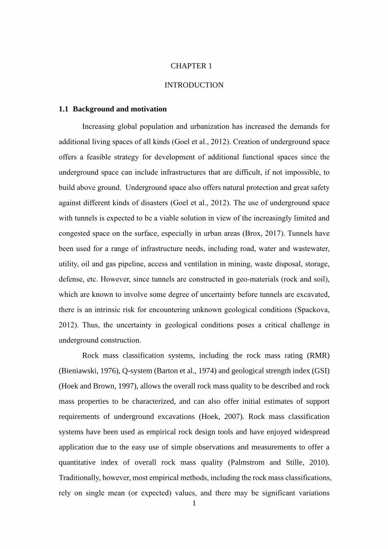
1.1 Background and motivation
Increasing global population and urbanization has increased the demands for
additional living spaces of all kinds (Goel et al., 2012). Creation of underground space
offers a feasible strategy for development of additional functional spaces since the
underground space can include infrastructures that are difficult, if not impossible, to
build above ground. Underground space also offers natural protection and great safety
against different kinds of disasters (Goel et al., 2012). The use of underground space
with tunnels is expected to be a viable solution in view of the increasingly limited and
congested space on the surface, especially in urban areas (Brox, 2017). Tunnels have
been used for a range of infrastructure needs, including road, water and wastewater,
utility, oil and gas pipeline, access and ventilation in mining, waste disposal, storage,
defense, etc. However, since tunnels are constructed in geo-materials (rock and soil),
which are known to involve some degree of uncertainty before tunnels are excavated,
there is an intrinsic risk for encountering unknown geological conditions (Spackova,
2012). Thus, the uncertainty in geological conditions poses a critical challenge in
underground construction.
Rock mass classification systems, including the rock mass rating (RMR)
(Bieniawski, 1976), Q-system (Barton et al., 1974) and geological strength index (GSI)
(Hoek and Brown, 1997), allows the overall rock mass quality to be described and rock
mass properties to be characterized, and can also offer initial estimates of support
requirements of underground excavations (Hoek, 2007). Rock mass classification
systems have been used as empirical rock design tools and have enjoyed widespread
application due to the easy use of simple observations and measurements to offer a
quantitative index of overall rock mass quality (Palmstrom and Stille, 2010).
Traditionally, however, most empirical methods, including the rock mass classifications,
rely on single mean (or expected) values, and there may be significant variations
2
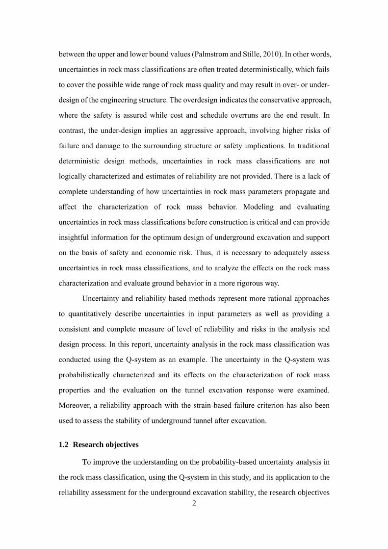
between the upper and lower bound values (Palmstrom and Stille, 2010). In other words,
uncertainties in rock mass classifications are often treated deterministically, which fails
to cover the possible wide range of rock mass quality and may result in over- or under-
design of the engineering structure. The overdesign indicates the conservative approach,
where the safety is assured while cost and schedule overruns are the end result. In
contrast, the under-design implies an aggressive approach, involving higher risks of
failure and damage to the surrounding structure or safety implications. In traditional
deterministic design methods, uncertainties in rock mass classifications are not
logically characterized and estimates of reliability are not provided. There is a lack of
complete understanding of how uncertainties in rock mass parameters propagate and
affect the characterization of rock mass behavior. Modeling and evaluating
uncertainties in rock mass classifications before construction is critical and can provide
insightful information for the optimum design of underground excavation and support
on the basis of safety and economic risk. Thus, it is necessary to adequately assess
uncertainties in rock mass classifications, and to analyze the effects on the rock mass
characterization and evaluate ground behavior in a more rigorous way.
Uncertainty and reliability based methods represent more rational approaches
to quantitatively describe uncertainties in input parameters as well as providing a
consistent and complete measure of level of reliability and risks in the analysis and
design process. In this report, uncertainty analysis in the rock mass classification was
conducted using the Q-system as an example. The uncertainty in the Q-system was
probabilistically characterized and its effects on the characterization of rock mass
properties and the evaluation on the tunnel excavation response were examined.
Moreover, a reliability approach with the strain-based failure criterion has also been
used to assess the stability of underground tunnel after excavation.
1.2 Research objectives
To improve the understanding on the probability-based uncertainty analysis in
the rock mass classification, using the Q-system in this study, and its application to the
reliability assessment for the underground excavation stability, the research objectives
3
in this report are as follows:
(1) Probabilistically characterize and predict uncertainties in rock mass classification
Q-system before tunnel excavation and validate the predicted results with rock mass
quality data collected during tunnel construction.
(2) Investigate the effects of uncertainties in input parameters in the Q-system on the
overall Q value and associated rock mass characterization and ground response
evaluation for underground structures.
(3) Perform reliability analysis with probabilistic Q-system on the basis of a strain-
based failure criterion to evaluate the tunnel excavation stability.
1.3 Report outline
This report is composed of six chapters, which are outlined below. All references
are placed at the end of the report.
Chapter 1 presents the general background, the motivation for this research,
research objectives and report outline.
Chapter 2 presents the literature review in the report. The commonly used
modern rock mass classification systems, sources of uncertainties in rock mass
classifications and treatment approaches are introduced. In addition, reliability-based
methods and the application in underground construction are also described.
Chapter 3 presents a rock mass classification Q-system-based prediction model
using the Markov Chain technique to probabilistically assess rock mass quality before
tunnel excavation. Based on the proposed prediction model, the probability distribution
of the overall Q value can be derived at arbitrary locations along the tunnel alignment
using Monte Carlo simulations. In addition, an analytical approximation approach to
deriving statistics (mean, standard deviation, and coefficient of variation) of the Q value
has also been developed given statistics of input parameters in the Q-system. The
proposed prediction model and analytical approach have been applied to a case study
of a water tunnel and validated by the actual Q value recorded during tunnel
construction.
Chapter 4 presents a paper titled “Monte Carlo simulation (MCS)-based
4
uncertainty analysis of rock mass quality Q in underground construction” This paper
has been published in The Journal of Tunneling and Underground Space Technology.
An MCS-based uncertainty analysis framework has been proposed to probabilistically
quantify the uncertainty in the rock mass classification Q-system. The proposed
framework has been implemented in the Shimizu highway tunnel case study. Based on
relative frequency histograms of Q-parameters (input parameters in the Q-system), the
probability distribution of the Q value is obtained using the MCS technique, which is
then used to probabilistically estimate rock mass properties and responses with
appropriate empirical correlations. The probabilistic estimates of rock mass properties
are also adopted as inputs in a finite element model for the probabilistic evaluation of
the excavation-induced tunnel displacement. In addition, the probabilistic sensitivity
analysis is conducted in the MCS process to identify the most important Q-parameters
in the Q-system based on several ranking criteria. The effects of correlation and
distribution types of input parameters in the probabilistic Q-system on the Q value and
associated rock mass parameters have also been investigated.
Chapter 5 presents a reliability assessment using the Q-based empirical
approach for the preliminary evaluation of the excavation stability using the FORM
algorithm. The probabilistic critical strain and the Q-based empirically estimated tunnel
strain are incorporated in the limit state function for reliability analysis. Reliability
analysis is also conducted using the MCS technique for comparison. The Shimizu
tunnel case study is also utilized as an example to perform reliability assessment on the
excavation stability. The effects of the correlation, distribution types and coefficient of
variation in input parameters on the reliability have also been investigated. The
reliability results on the stability evaluation of the excavated tunnel have been
compared to those derived using analytical and numerical approaches.
Chapter 6 is the final chapter of this report. Major findings and conclusions are
summarized, and directions for future work are also presented.
5
CHAPTER 2
LITERATURE SURVEY
This chapter presents the literature review for this research, which mainly includes
uncertainty analysis in rock mass classification systems and reliability-based
assessment in underground construction. The commonly used rock mass classification
systems, involved uncertainties and treatment approaches have been introduced.
Reliability-based methods, the comparison with factor of safety and reliability
assessment in underground construction are also presented.
2.1 Uncertainty analysis in rock mass classification systems
2.1.1 Rock mass classification system
Rock mass classification involves the process of placing rock masses into groups
or classes based on defined relationships and has played an indispensable part in
engineering design and practice (Bieniawski, 1989). Rock mass classification systems
provide a basis for understanding the characteristics and behavior or rock mass, serving
as the basis of the empirical design and relating to experiences obtained in rock mass
conditions at one site to another. The objectives of the rock mass classification are
proposed (Bieniawski, 1989):
(1) Identify the most important parameters impacting the rock mass behavior.
(2) Subdivide a particular rock mass formation into groups or classes of similar
behavior.
(3) Provide a basis for understanding the characteristics of each rock mass class.
(4) Relate the experience of rock mass conditions at one site to the conditions and
experience gained at another.
(5) Derive quantitative data and guidelines for rock engineering design, e.g. support
guidance for underground excavations.
(6) Provide a common basis for communication between engineers and geologists
The advantages of rock mass classifications have also been summarized(Bieniawski,
1989):

6
(1) Rock mass classification systems can provide a checklist for the ground parameters
to be collected, thus improving the quality of site investigation
(2) Classification systems can provide quantitative information for engineering design
purposes
(3) These quantitative classifications enable better engineering judgement and more
effective communication on a project.
Problems in the application of rock mass classifications arise when (Bieniawski,
1993):
(1) Using rock mass classification as the ultimate design solution, i.e. neglecting the
analytical, numerical and observational methods;
(2) Using on rock mass classification only without cross-checking with other
classification systems
(3) Using rock mass classification without sufficient input data
(4) Using rock mass classifications without realizing the conservatism and limits arising
from the databases on which they are based.
Commonly used rock mass classification systems are briefly introduced below,
namely the RMR system, Q-system and the GSI system.
RMR system
The Geomechanics Classification or the RMR system was developed by
Bieniawski (1976) to evaluate the excavation stability and support requirements of
tunnels. Since then it has been improved based on more collected case histories, and
the 1989 version of the classification is introduced herein. The RMR system has six
input parameters, i.e. uniaxial compressive strength (UCS) of rock material, rock
quality designation (RQD), the spacing of discontinuities, condition of discontinuities,
groundwater conditions and the orientation of discontinuities (Bieniawski, 1989).
Ratings are given to each input parameter, and the summation of these ratings is the
overall RMR value.
In applying the RMR system, the rock mass is subdivided into a number of
structural zones (Bieniawski, 1989). Each zone is relatively geologically homogeneous
7
and classified separately. A major structural feature such as a fault or the change of
rock types may be considered as the boundary of structural zones (Hoek, 2007). In
terms of the application of the RMR system, it provides a set of guidelines for
excavation and support of 10 m span rock tunnels constructed using drill and blast
methods (Hoek, 2007). The RMR is also applied to estimate the unsupported span and
stand-up time for excavated tunnels. In addition, the RMR system can also be used to
estimate rock mass properties based on some empirical correlations (Bieniawski, 1989).
Q-system
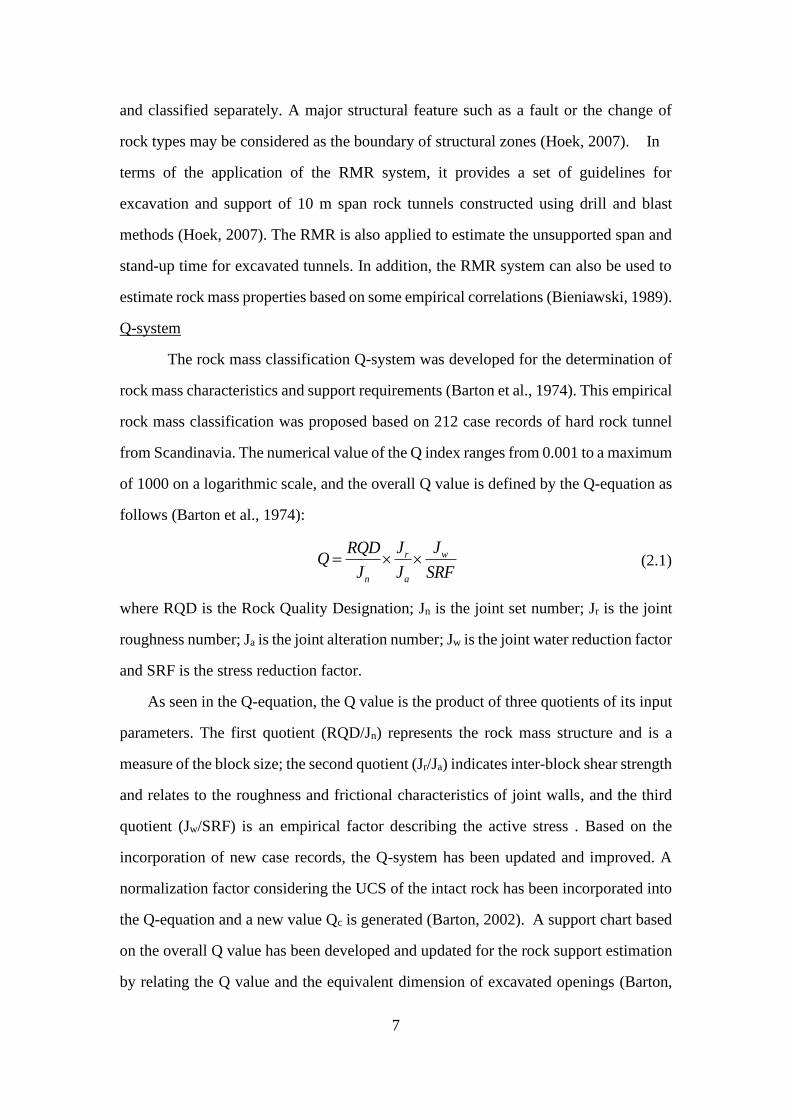
The rock mass classification Q-system was developed for the determination of
rock mass characteristics and support requirements (Barton et al., 1974). This empirical
rock mass classification was proposed based on 212 case records of hard rock tunnel
from Scandinavia. The numerical value of the Q index ranges from 0.001 to a maximum
of 1000 on a logarithmic scale, and the overall Q value is defined by the Q-equation as
follows (Barton et al., 1974):
wr
n a
JJRQDQ
J J SRF= (2.1)
where RQD is the Rock Quality Designation; Jn is the joint set number; Jr is the joint
roughness number; Ja is the joint alteration number; Jw is the joint water reduction factor
and SRF is the stress reduction factor.
As seen in the Q-equation, the Q value is the product of three quotients of its input
parameters. The first quotient (RQD/Jn) represents the rock mass structure and is a
measure of the block size; the second quotient (Jr/Ja) indicates inter-block shear strength
and relates to the roughness and frictional characteristics of joint walls, and the third
quotient (Jw/SRF) is an empirical factor describing the active stress . Based on the
incorporation of new case records, the Q-system has been updated and improved. A
normalization factor considering the UCS of the intact rock has been incorporated into
the Q-equation and a new value Qc is generated (Barton, 2002). A support chart based
on the overall Q value has been developed and updated for the rock support estimation
by relating the Q value and the equivalent dimension of excavated openings (Barton,
8
2002; Barton et al., 1974; Grimstad, 1993). Relationships between the Q value and the
seismic velocity, depth, deformation modulus of rock mass, required support pressure,
have been developed, and these parameters can be roughly estimated using the
empirical correlations based on obtained Q value (Barton, 2002).
GSI system
The GSI system was introduced to estimate the reduction in rock mass strength
under different geological conditions (Hoek and Brown, 1997). The GSI can be
estimated based on field observation and geological descriptions by combing the rock
mass structure (block size) and the rock discontinuity surface conditions (roughness
and alteration). It is also recommended to use a range of GSI values rather than single
number or value (Hoek, 1998a). The GSI has been modified to cover more complex
geological conditions, such as shear zones or heterogeneous rock masses, and the GSI
chart are updated to incorporate these categories (Hoek and Marinos, 2000a; Hoek et
al., 1998). In addition, the GSI system has been interpreted in a more quantitative
manner by many authors (Cai et al., 2004; Hoek et al., 2013; Hoek et al., 1998; Marinos
et al., 2005).
In terms of the application, the GSI system has been used to estimate the rock
mass properties in rock engineering (Hoek et al., 2002; Marinos and Hoek, 2000). It
also serves as a tool to estimate the parameters in the Hoek-Brown criterion of rock
masses (Hoek and Brown, 1997; Hoek et al., 2002).
2.1.2 Sources of uncertainty in rock mass classification system
Uncertainty can be categorized as aleatory or epistemic uncertainty (Baecher
and Christian, 2003). Aleatory uncertainty relates with the natural, intrinsic randomness
which may be dealt with probabilistic or statistical analysis. In contrast, the epistemic
uncertainty results from incomplete knowledge and can be reduced when additional
information is available. Einstein and Baecher (1983) also divided the sources of
uncertainty in geotechnical engineering as: (1) inherent spatial and temporal variability;
(2) measurement errors; (3) model uncertainty; (4) load uncertainty; and (5) omissions.
9
Rock mass classification systems are based on experience and thus have similar
inherent uncertainties (Stille and Palmström, 2003). Input parameters in the rock mass
classification have inherent uncertainties due to the spatial variability and heterogeneity
of rock mass itself. The determination of the ratings for input parameters in the rock
mass classification systems also involves uncertainty. For example, RQD can often lead
to a sampling bias due to a preferential distribution of joints (Grenon and Hadjigeorgiou,
2003). In addition, uncertainties also take place in observing and recording joint
characteristics. The mapping results for the joint location for different observers along
the same scanline are very different (Ewan et al., 1983). Some input parameters relating
to joint features in the rock mass classifications are prone to mischaracterization
(Palmstrom and Broch, 2006).
Hadjigeorgiou and Harrison (2011) also noted that rock mass classification
systems have uncertainties and not considering them may lead to statistical errors. Two
groups of errors can be generated in the use of rock mass classifications. The first group
relates with the intrinsic errors in the rock mass classifications, such as the errors of
omission, errors of superfluousness, and errors of taxonomy. The omission means the
failure to consider pertinent characteristics in rock mass classifications, such as the
absence of UCS in the Q-system and the in-situ stress condition in the RMR system.
The consideration of rock mass anisotropy is also omitted in both RMR and the Q-
system. With regard to the superfluousness, the RQD and discontinuity spacing are a
good example since these two parameters are not mutually independent, indicating that
either can be estimated from the other. The errors of taxonomy are due to the
requirement to pick a number or rating value for a geomechanical property. For
example, for the joint water reduction factor Jw in the Q-system, it is not clear how to
classify “medium inflow with significant outwash of joint fillings”. In contrast to the
first group of error types, the second group is associated with implementation, such as
the errors of human error and errors of ignoring variability or uncertainty. The
assignment of only one value, instead of a range of distribution, ignores the
heterogeneous and random nature of rock mass properties. The risk analysis for a
10
certain rock engineering project also depends on the level of confidence in known
relevant parameters, which is dependent on the amount of available information, the
variation of input parameters in rock mass classifications and its impact on the probable
rock mass quality index and the required minimum rock mass quality for compatibility
with proposed excavation requirements (Carter, 1992).
2.1.3 Dealing with uncertainty in rock mass classification system
Empirical assessment methods, including those based on rock mass
classification systems, are essentially deterministic approaches (Carter, 1992).
However, the use of only one subjectively assigned value cannot consider the wide
range of actual rock mass characteristics that are often encountered in engineering
practice. It is appropriate to provide a range of values, instead of a single value, to each
input parameter in rock mass classification systems and to assess the significance of the
final result (Hoek, 2007). The obtained mean value can be used in choosing the basic
rock support while the range can provide an indication of the possible adjustments that
may be required to meet different conditions encountered during tunnel excavation. It
is also recommended by Hoek (1998a) that a range of values of GSI should be used in
preference to a deterministic value. Barton et al. (1994) have used the Q-histogram
logging approach to collect the histogram of input parameters in the Q-system, and
statistics (min, max, mean, and mode) of the Q value can be obtained using the interval
analysis. However, Panthi (2006) pointed out that the mean and range values have poor
statistical properties and are sensitive to extreme values. Similarly, Bedi (2013) also
stated that the possible wide range of Q value intervals lacks sufficient information and
may cause difficulty in decision-making. Carter (1992) suggested that it is
advantageous to replace the subjectivity associated with a selecting single value with
the use of probabilistic sampling approaches accounting for the uncertain and variable
nature of rock masses. These probabilistic approaches can provide some insights into
the degree of uncertainty in the input parameters in the rock mass classifications. Carter
(1992) also stated that geological-geomechanical factors, such as rock strength and rock
structure, are particularly amenable to the probabilistic treatment and that it is
11
advocated to evaluate the collected geotechnical site investigation data for rock
engineering projects from a probabilistic point of view. The probabilistic approach in
evaluating rock mass classifications, rather than straightforward use of deterministic
assessment, can provide the designer not only with a better understanding on the
sensitivity of the output to variations in the input parameters, it also reflect the basic
uncertainties inherent in the rock mass parameter data on which the design is predicated
(Carter, 1992). If the uncertainty and variability in the rock mass classifications are not
sufficiently characterized, they might propagate through the analysis and design
process and adversely impact the ground response and support performance (Langford,
2013).
Fortunately, probabilistic evaluation on the rock mass classification, which
enables the description of the complete probability distribution function (PDF) of rock
mass parameters, is capable of quantifying the uncertainty and its effect on the design
performance. Cai (2011) presented that both the intrinsic and subjective uncertainties
in rock mass classifications can be captured in the probabilistic evaluation and the
probabilistic design can be accordingly conducted. Bedi (2013) derived the probability
density function of the Q value in the Gjovik cavern using the Monte Carlo simulation
(MCS) method based on the assumed triangular distributions of Q-parameters. Carter
(1992) also performed similar simulations to derive the distribution of the Q value and
suggested that simple triangular distributions often provide sufficient accuracy. Panthi
(2006) assumed the normal or lognormal distributions for RQD, Jr and Ja parameters
while the triangular distributions for Jn, Jw and SRF parameters in the Q-system, and
the PDF of the Q value was obtained using the MCS technique for the Himalayan
mountainous tunnels. Analogously, the distribution of GSI was also estimated from the
statistical distributions of joint characteristics in field mapping, which was then used as
the input in the numerical model for probabilistically evaluating the excavation
response and stability of underground construction (Cai, 2011; Idris et al., 2015; Tiwari
et al., 2017). The probability distributions of RMR and GSI were derived based on the
probabilistic descriptions of discontinuities and intact rock properties using the MCS
12
technique, and the strength and deformability properties of rock mass were also
probabilistically estimated based on some empirical relationships (Sari, 2009; Sari et
al., 2010).
However, few researchers have investigated the contributions of input
parameters in the rock mass classification systems within a probabilistic framework. In
addition, the majority of studies fail to consider the interdependency between uncertain
input parameters and its impact in rock mass classifications. Further, although rock
mass parameters are amenable to probabilistic treatment, few studies have examined
the effects of distribution types of input parameters in rock mass classifications on the
overall rock mass quality and associated rock mass characterization and response.
2.2 Reliability-based assessment in underground construction
2.2.1 Factor of safety and reliability concept
Traditionally, the deterministic factor of safety (FS) is applied to deal with the
uncertainties in the geotechnical engineering. The factor of safety is calculated as the
ratio of characteristic resistance over the characteristic load. The characteristic
resistance and load are conservative estimates of resistance and load in the system
(Fenton and Griffiths, 2008). When the characteristic values are equal to the means,
then the factor of safety can be defined in terms of the mean resistance and mean load:
R
Q
FS
= (2.2)
where FS is the factor of safety, R is the mean resistance, Q is the mean load.
Griffiths and Fenton (2007) stated that all uncertainty is lumped into the single
factor of safety, and the factor of safety does not provide information on the level of
safety in the design. The same factor of safety can generate two designs that have
different levels of safety. This may be due to factors of safety agreed on in design codes
or standards not being calibrated to each other. It is also common to apply the same
factor of safety for a given type of geo-structures, such as long-term slope stability,
without considering the uncertainties involved in the calculation (Duncan, 2000).
13
Fenton and Griffiths (2008) stated an example of three geotechnical designs, having the
same mean factor of safety, can have considerably different probabilities of failure. The
actual design safety is not adequately reflected in the mean factor of safety. Tapia et al.
(2007) also showed an example of slope design A and B, in which the FSA (1.35) is
smaller than the FSB (1.50). However, the greater uncertainty in design B, indicated by
larger spread, results in higher probability of failure despite the larger FS value in
design B in comparison to design A. This is an example for the slope design, however,
it can be equally applicable to underground construction.
The factor of safety in the conventional geotechnical engineering is generally
determined heuristically, based on experiences of similar projects. However, as
questioned by Griffiths and Fenton (2007), what if we do not have experience, such as
using new construction materials or in a new environment? What if the experience that
we have is not positive? The traditional factor of safety approach cannot answer the
above questions. Griffiths and Fenton (2007) also suggested that it is difficult to pick
an optimum factor of safety since the FS has no real meaning in terms of reliability.
The ambiguous nature of the factor of safety has also been reported by Low and
Einstein (2013), and two different definitions on the factor of safety against the wedge
falling were discussed. Each definition has its rationale while the values of FS can differ
by an order of magnitude. Lilly and Li (2000) also stated that the factor of safety, by
definition, is a binary criterion. Either the excavation is stable (FS>1) or fails (FS<1)
due to the fact that excavations at limit equilibrium (FS=1) are very rare in practice.
Zhang and Goh (2012) also pointed out that failure in underground excavation may
occur even when the FS is larger than 1.0.
To overcome these issues, reliability-based approaches have been developed to
provide a more consistent and complete measure of the safety level considering the
uncertainties involved. The subsection below will briefly introduce the reliability
theory.
2.2.2 Overview of reliability theory
(1) The general case
14
The performance function G(X) is used to describe the performance of
geotechnical structures, which also defines the acceptance criterion for the system in
terms of the limit state function (where X is the collection of all relevant input random
variables).The resistance R(X) and the load acting on the system Q(X) can be used to
construct the performance function, and the relationship can be expressed as follows:
( ) ( ) ( )G X R X Q X= − (2.3)
The critical limit state, indicated by G(X) = 0, defines the boundary between
safe and unsafe regions. G(X) > 0 means stable conditions are expected while G(X) <0
indicates the system has failed to meet the acceptance criterion.
Note that in underground construction, the resistance and load can rarely be
separated since the ground response depends on the support type and installation
sequence. The performance function can therefore be expressed with respect to a
limiting value for the ground response parameter (e.g. displacement, strain, plastic
radius) (Langford, 2013).
The probability of failure, or the probability of unsatisfactory performance, can
be defined as:
( ) 0[ ( ) 0] ... ( )f X
G Xp P G X f x dx
= = (2.4)
where ( )Xf x is the joint probability density function of the collection of random
variables X. This integral is generally non-tractable or impossible to solve analytically
when many random variables are involved. Thus, approximate methods, including First
Order Second Method (FOSM), First Order Reliability Method (FORM), Point
Estimate Method (PEM) and Monte Carlo Simulation (MCS), are used to evaluate the
integral.
(2) Reliability index
In geotechnical engineering, the safety margin M is defined as the difference
between the resistance R and the load Q (Baecher and Christian, 2003).
M R Q= − (2.5)
15
The mean value of the safety margin M is
M R Q = − (2.6)
where M , R , Q are the mean value of safety margin M, the resistance R, and the
load Q, respectively.
The variance of the safety margin M is
2 2 2 2M R Q RQ R Q = + − (2.7)
where M , R , Q are the standard deviation (SD) of the safety margin M, the
resistance R and the load Q, respectively; RQ is the correlation coefficient between R
and Q.
The reliability index is defined as:
2 2 2
R QM
M R Q RQ R Q
−= =
+ − (2.8)
The probability of failure pf can be given according to the following equation
based on the assumption that the safety margin M is normally distributed.
( 0) ( ) 1 ( )fp P M = − = − (2.9)
where pf is the probability of failure, ( ) is the cumulative distribution function of the
standard normal variable, is the reliability index.
Unlike the factor of safety, the reliability approach enables the consideration of
uncertainties in the input parameters and the level of safety and reliability can be
quantified. Based on this, consistent levels of reliability can be achieved among
different designs. In addition, different to the experience-based factor of safety, the
reliability-based approach can provide the ability to develop new designs which achieve
a specified reliability target. Moreover, by quantifying the reliability, the cost-benefit
analysis can also be carried out to balance the construction costs against the risk of
failure (Griffiths and Fenton, 2007).
16
However, despite the advantages of the reliability approach over the traditional
factor of safety, reliability approaches have not yet gained widespread application in
geotechnical practice. There are two main reasons (Duncan, 2000): first, reliability
theory contains some statistical terms that may not be very familiar to geotechnical
engineers; second, there is misconception that the application of the reliability approach
requires more data, time and effort than the traditional geotechnical analysis. Duncan
(2000) stated that simple reliability analyses, which require neither complex theory nor
unfamiliar statistical terms, require minimal additional effort compared to the
conventional analyses and should be used in geotechnical practice. Several example
applications were used to illustrate the simplicity and practicality of the reliability
approach. It has also been advocated that the reliability approach should complement,
instead of replacing, the factor of safety analyses in providing measures of acceptable
geotechnical design (Duncan, 2000).
2.2.3 Reliability-based methods
The following subsections describe the reliability methods that are commonly
used in reliability analysis and reliability-based design in underground structures. These
reliability methods can account for the effects of the variability of input parameters on
the resulting output variable, including the First Order Second Moment (FOSM), the
First Order Reliability Method (FORM), the Point Estimate Method (PEM) and the
Monte Carlo simulation (MCS).
FOSM
The FOSM method uses the first terms of a Taylor series expansion of the
performance function to evaluate the mean value and variance of the performance
function (Baecher and Christian, 2003). The Taylor expansion is truncated after the
linear term, and this is called the first order. The first two moments of the output
variable are to be estimated, in which the variance is a form of the second moment and
the highest order statistics in the analysis, and this is termed as second moment (Fenton
and Griffiths, 2008). If the number of the random variable is N, this method needs either
17
estimating N partial derivatives of the performance function or performing a numerical
approximation with evaluations at 2N+1 points (Baecher and Christian, 2003).
The FOSM method is relatively simple and widely used since it requires the
evaluation of a minimal number of terms and only the first statistic moments are needed.
The evaluation points in the FOSM method are similar to those that are used in
parametric sensitivity analysis, thus the contributions of each input parameter can also
be revealed (Langford, 2013). However, it should be noted that the accuracy of the
FOSM method deteriorates caused by the truncation of the Taylor expansion series after
the linear terms if the second and higher derivatives of the performance function are
significant, e.g. in situations where the performance functions are highly non-linear
(Fenton and Griffiths, 2008). In addition, the probability distribution functions are not
taken into account for input parameters, and only the mean and standard deviation are
used, which may also result in the approximation errors. Moreover, different values for
the probability of failure are obtained using different performance functions for the
same problem, indicating the non-uniqueness and inconsistency of reliability evaluation
using FOSM (Baecher and Christian, 2003).
FORM
To overcome the problems in the FOSM method, the FORM method was
developed by Hasofer and Lind (1974) based on a geometric interpretation of the
reliability index as a measure of the distance in dimensionless space between the mean
point of the multivariate distribution of input parameters to the boundary of limit state
surface. The point where the reliability index ellipsoid touches the limit state surface is
termed the design point. A spreadsheet method using the SOLVER add-in with the
optimization routine for the Excel can be efficiently used to determine the reliability
index in the reliability analysis (Low and Tang, 1997). The distribution types for the
input random variables can be defined, and the correlation structure between variables
can be captured by the correlation coefficient matrix. The probability of failure can also
be approximated based on the assumption that the performance function is normally
distributed.

18
The design point in the FORM spreadsheet, i.e. the x* value, indicates the most
likely failure point on the limit state surface. The distance between the design point and
the mean value point of each input parameter reflects the sensitivity of the performance
function to that input variable. The ratio of the mean value to the design point value (x*)
is also similar to the partial factor in limit state design in Eurocode 7. However, the
partial factors are specified in Eurocode 7 while the design point values are determined
automatically in the FORM spreadsheet. The design point values can reflect
sensitivities, correlation structures, standard deviations, and probability distributions in
a fashion that the prescribed partial factors cannot reflect (Low, 2008b).
PEM
The PEM method was proposed by Rosenblueth (1975) to approximate the
mean and standard deviation of the performance function. It is used to obtain the
statistical moments of the performance function by evaluating at a set of selected points.
The PEM method is a weighted average method, and solutions at different evaluation
points are combined with proper weights to get an approximation of the statistic
moments of the output variable. The two-point estimate method for the first two
moments of uncorrelated random variables is commonly used, and sampling points are
selected at one standard deviation above and below the mean value of each random
variable. If the performance function has N random variables, then there will be 2N
sampling points considering all combinations of evaluation points (Fenton and Griffiths,
2008). If all random variables are uncorrelated, then the weight value is simply 1/2N for
each random variable (Langford, 2013).
The PEM method is preferable to other methods for cases with five or fewer
random variables in terms of computation efficiency. However, the number of 2N
evaluations can be a very large number if many random variables are involved. In
addition, as with FOSM method, it does not account for the probability distribution off
the performance function. Generally the normal distribution is assumed both for the
input and output variable. Further, little information is known about the low probability
conditions since the performance function is only evaluated at one standard deviation
19
above and below the mean value. In other words, values beyond the bounds are not
considered and these low probability events outside of the bounds may lead to high
consequences, thus posing a great risk to the design (Langford, 2013). It is also noted
that the PEM method does not perform well in capturing mixed behavior or mode
switches since the abrupt change in behavior will not be detected in the PEM (Valley
et al., 2010).
MCS
In situations where the performance function is complicated and difficult to
assess, the probability of failure can be evaluated directly using the MCS simulation
technique. The distributions of the input parameters should be assigned first, and then
single values of the input variables are randomly sampled in one iteration according to
their respective distributions. This set of sampled input values are then used to calculate
a value of the output parameter. With a number of iterations, more input values are
sampled and accordingly a number of output values are generated. The statistical
moments of the output can be estimated and an appropriate distribution function can be
determined for the output variable. Based on the obtained distribution of the
performance function, the probability of failure can be calculated as the probability that
the performance function is less than or equal to zero.
The MCS technique is straightforward and has the advantage of conceptual
simplicity. The distributions for the input parameters can be specified based on the
collected information, and the correlation structure between input variables can also be
captured. The major disadvantage is that it is computationally expensive and time
consuming. The computation efforts are extremely high if adequate accuracy of
calculation is to be satisfied especially when the estimated probability of failure is very
low (Baecher and Christian, 2003). The considerable computational effort can be
reduced using variance reduction techniques in which the accuracy level is sustained
while the required number of computations is reduced. The MCS simulation can be
used as a complement to discrete sampling methods to ensure an accurate evaluation of
the system performance especially for complex problems (Langford, 2013).
20
2.2.4 Reliability evaluation in underground construction
Uncertainties are unavoidable in geotechnical engineering, including
underground construction, and they stem from loads, geotechnical properties,
measurement errors, calculation models etc. (Ang and Tang, 2007; Baecher and
Christian, 2003). The limitations of the FS-based design approach, which has been
traditionally used in the geotechnical practice, have been pointed out, and alternatives
including the partial factor design in Eurocode 7 and the load and resistance factor
design (LRFD) approach in United States, which is equivalent to limit state design
(LSD) in Canada, have been developed (Ang and Tang, 2007; Baecher and Christian,
2003; Fenton and Griffiths, 2008). The LRFD, LSD and partial factor approaches, are
philosophically similar and the focus is the re-distribution of the factor of safety into
separate load and resistance factors or partial factors for ground parameters (Phoon et
al., 2003).
The LRFD approach subjectively incorporates uncertainties of load and
resistance into the design process by assigning separate factors to each. The LRFD
approach has been used extensively in North America for geotechnical structures, in
which the prescribed limit state in LRFD should yield a constructed system having a
target reliability or an acceptable probability of failure (Fenton and Griffiths, 2008).
The LRFD is used relatively straightforward in gravity-driven structures, such as the
foundation and retaining wall design, as the loads and resistances can be considered
separately in the design (Langford, 2013). However, the LRFD approach is more
complicated in underground structures. The system performance is defined by the
relationship between deformations, loads that have been induced by rock mass stresses,
and the capacity of support elements, thus limiting its applicability in the underground
works (Langford, 2013). Fortunately, reliability methods are capable of assessing how
uncertainty in rock mass parameters propagates through the analysis and design to
obtain a measure of uncertainty in the system performance. The reliability-based
approach provides a more consistent and complete measure of risk since it not only
defines the expected case (as with a deterministic analysis) but it also provides a
21
measure of design performance based on the probability of failure (Langford, 2013).
The reliability-based approach using the FORM spreadsheet with an expanding
ellipsoid has the ability to seek the most-probable design point without presuming any
partial factors and to automatically reflect sensitivities from case to case (Low, 2008b).
The superiority of reliability-based methods to approaches including the traditional
factor of safety, LRFD and the partial factor approach is summarized in (Phoon et al.,
2003).
Despite its benefits, the reliability analysis in the geotechnical engineering has
been focused on surface geotechnical projects and has not yet achieved widespread in
the design of underground construction (Langford 2013). While some productive
research has been done on the reliability analysis in underground construction
(Bjureland et al., 2017; Langford and Diederichs, 2013; Liu and Low, 2017; Low and
Einstein, 2013; Mollon et al., 2009a, b, 2010), more attention should be paid to some
issues in this area. To start with, the reliability analyses in the current research are
mostly based on analytical solutions or numerical procedures. However, in the
analytical solutions, the ground-support interaction is often used to establish the
performance function, and this is always based on some simplistic assumptions that are
rarely met in practice (Li and Low, 2010; Su et al., 2011). For example, the
convergence-confinement method (Carranza-Torres and Fairhurst, 2000; Panet and
Guenot, 1983) was adopted by Li and Low (2010) to construct the performance function
of tunnel response for reliability analysis, in which a circular tunnel was assumed to be
subjected to hydrostatic stresses with uniform internal pressure around the tunnel
perimeter. Due to the implicit characteristics of the performance function in
underground construction, numerical procedures with finite element or finite difference
models using different algorithms have been used to construct the limit state function,
including the response surface method (Hamrouni et al., 2017; Lü et al., 2011; Mollon
et al., 2010), regression methods (Basarir, 2008; Zhang and Goh, 2015; Zhu et al., 2008),
artificial neural networks (Adoko et al., 2013; Lü et al., 2012; Mahdevari and Torabi,
2012), support vector machines (Tan et al., 2011; Zhao, 2008; Zhao et al., 2014) and

22
radial basis functions (Bai et al., 2012; Fang et al., 2005; Wang et al., 2016). However,
the numerical procedures are generally computationally expensive, which requires a
great deal of computational effort. In addition to the analytical and numerical
procedures, some empirical relationships or evidences with regard to tunnel response
(e.g. displacement, strain, and plastic radius) have also been developed to evaluate the
excavation stability (Barton, 2002; Barton et al., 1994; Marinos and Hoek, 2000;
Sakurai, 1983). However, no current research has adopted such empirical correlations
in reliability evaluation to preliminarily assess the stability of underground excavations.
In addition, the focus of the majority of the research is the illustration of the newly
proposed reliability analysis approaches or algorithms, and hypothetical examples are
generally used with assumed statistical data of rock mass parameters, indicating few
case studies with real rock mass parameter data have been adopted to validate proposed
approaches or algorithms. Moreover, previous work has focused only on the
deterministic critical strain using the strain-based limit state function in the reliability
assessment on underground construction. In other words, the previous work failed to
consider the uncertainty in the critical strain itself.
23
CHAPTER 3
A STUDY OF A PROBABILISTIC Q-SYSTEM USING A MARKOV CHAIN
MODEL TO PREDICT ROCK MASS QUALITY IN TUNNELING
3.1 Abstract
Uncertainties in rock mass conditions are mainly caused by the inherently
inhomogeneous nature of rock masses. Assessment of rock mass quality without
accounting for inherent uncertainty often leads to excessive conservatism in design and
construction, resulting in a negative effect on overall design and construction processes;
thus, accurate prediction of rock mass quality is critical to save project cost and time.
In this study, to advance rock mass quality assessment, a Q-based prediction model to
assess probabilistic rock mass quality has been proposed using the Markov chain
technique with quantitatively characterized uncertainties. Based on the Markovian
prediction model, the statistical distribution of the Q value has been derived from
arbitrary locations along a tunnel alignment using Monte Carlo simulations. The
predicted results derived using the proposed probabilistic prediction model have also
been compared to those obtained using the deterministic prediction approach. In
addition, an analytical approximation approach to deriving the statistics (mean,
standard deviation, and coefficient of variation) of the Q value given statistics of Q-
parameters has also been developed. In this study, the proposed prediction model and
analytical calculation approach were applied to a case study of a water tunnel and have
been validated by the actual Q values recorded during construction. The proposed Q-
based prediction model is capable of assessing the rock mass quality of unexcavated
tunnel sections using a probabilistic approach, thus serving as a supplement to geologic
exploration and prospecting in planning and preliminary design stage. The proposed Q-
based model is also useful in evaluating excavation support strategies as well as
construction time and cost, providing decision support for the optimization of tunnel
design and construction.
24
3.2 Introduction
Accurate prediction of rock mass conditions is a main focus in the underground
construction and tunneling industry (Haas and Einstein, 2002). However, most
subsurface rock mass conditions are not sufficiently known before construction. In
general, rock mass conditions have been mostly evaluated for the worst-case scenario
in traditional deterministic analyses, leading to biased conclusions since the inherent
uncertainty of the rock mass conditions is not considered, resulting in serious
construction delays and cost overruns of projects (Langford, 2013; Sousa and Einstein,
2012). In contrast, if this uncertainty is well modeled and analyzed before construction
start, it can help significantly reduce risks as well as project costs, providing proper
decision support for excavation-support strategies (Spackova, 2012).
Many geologic prediction techniques, such as geostatistical approaches and
Markov models, have been developed to assess geological uncertainty in tunneling and
underground construction (Chan, 1981; Chen et al., 2017; Ferrari et al., 2014; Ioannou,
1987; You and Lee, 2006). The Markov process approach is of particular interest
because geological processes can be well addressed by the Markov process (Chan, 1981;
Guan et al., 2012; Ioannou, 1987). Chan (1981) has shown that geological parameters
can be probabilistically predicted using the Markov Chain technique. In addition, the
Markov process approach has some advantages over semivariogram and
autocovariance-based geostatistical methods because a Markov chain model can be
implemented with limited data (less than ten boreholes) to simulate geological
uncertainty, whereas variograms or autovariance functions require a great amount of
data, e.g. more than tens of boreholes (Qi et al., 2016). Additionally, the transitional
probability used in the Markov process approach can be geologically interpreted more
easily than the variogram or autocovariance function, contributing to the popularity of
the Markov model (Carle, 2000; Elfeki and Dekking, 2001; Elfeki and Dekking, 2005;
Guan et al., 2012; Park et al., 2005; Ye and Khaleel, 2008). For these reasons, the
Markov process has been widely used for geologic predictions in diverse fields in
25
geotechnical engineering (Bi et al., 2015; Elfeki and Dekking, 2001; Felletti and Beretta,
2009; Haas and Einstein, 2002; Min et al., 2008; Ruwanpura et al., 2004).
In the field of underground construction, the ground is often described behaviorally
and allocated a ground class based on the field observations (Stille and Palmström,
2003). However, as a descriptive and behavioral system, the documentation of ground
conditions in some ground classifications based on field observations does not seem to
be very clear since the ground classifications rely largely on subjective observations
(Palmstrom and Stille, 2007). The rock mass is subjectively classified without a
numerical quality rating; in other words, the ground conditions are described
qualitatively (Bieniawski, 1989). In addition, a limited number of geologic parameters
and parameter states are generally used to characterize the ground conditions, which
may lead to inadequate evaluation of the overall rock mass conditions. For instance,
only two parameters (the N value in the standard penetration test and the percentage of
clay content) were used to describe geologic classes (Leu and Adi, 2011), and only two
fuzzy states (severe and not severe) were adopted to characterize weathering grades
(Ioannou, 1987). Thus, the importance of some geological input parameters in ground
classification seems to be ignored in current research and practice. Additionally,
interdependency or correlation among geological input parameters in ground
classifications is disregarded (Leu and Adi, 2011). Often, a ground classification is
determined by several case-dependent geologic parameters based on a specific
individual project. However, most of the aforementioned limitations of ground
classification can be overcome using a probabilistic Q-system.
The Q-system — proposed by (Barton et al., 1974) in the Norwegian Geotechnical
Institute (NGI) for the design of support in underground excavations — is a quantitative
rock mass classification system. As an empirical method, the Q-system has been
developed based and updated on a large number of case histories and updates of global
tunneling projects and contains six parameters that are critical during underground
construction (Hoek, 2007). Each input parameter of the Q-system has several states
with different numerical values, which provides relatively complete descriptions of
26
ground conditions (Hoek, 2007); thus, the Q-system as a quantitative rock mass
classification system has an advantage relative to the qualitative ground classifications.
In the Q-system, the numerical Q value can be calculated with individual ratings
assigned to each input parameter within its range according to the Q-equation (Barton
et al., 1974). Consequently, sensitivity analyses can be performed by investigating the
effect of each Q-parameter on the overall Q value by changing one parameter while
keeping the other parameters constant. The correlation among the Q-parameters can be
quantitatively characterized in the Q-equation. Furthermore, in the Q-based support
chart, several rock classes and possible support patterns have been defined with
extensive case histories and updates (Barton, 2002; Barton et al., 1974; Grimstad, 1993),
and a support pattern can be determined from the obtained Q value. Empirical rock
mass classification systems, including the rock mass rating (RMR), the Q-system and
the geological strength index (GSI), have inherent uncertainties (Palmstrom and Stille,
2007; Palmstrom and Stille, 2010). However, it is possible to probabilistically
characterize the uncertainties in the Q-system and to specify the excavation support
strategies using the Q-based rock classes in a probabilistic way.
The Q-system is advantageous over the ground classification in quantitatively
characterizing the rock mass conditions, which accounts for the inherent uncertainty
involved. Thus, in this chapter, a Q-based prediction model for rock mass quality is
proposed with the Markov process prediction approach by considering the uncertainties
in the Q-system. We have demonstrated that the proposed Q-based prediction model is
capable of the quantitative prediction of rock mass quality before tunnel excavations
with a probabilistic method, providing useful information not only for assessing
excavation support strategies but also for saving project time and cost in underground
construction and tunneling.
3.3 Methodology
3.3.1 The Markovian prediction approach
Markov process and Markov chain
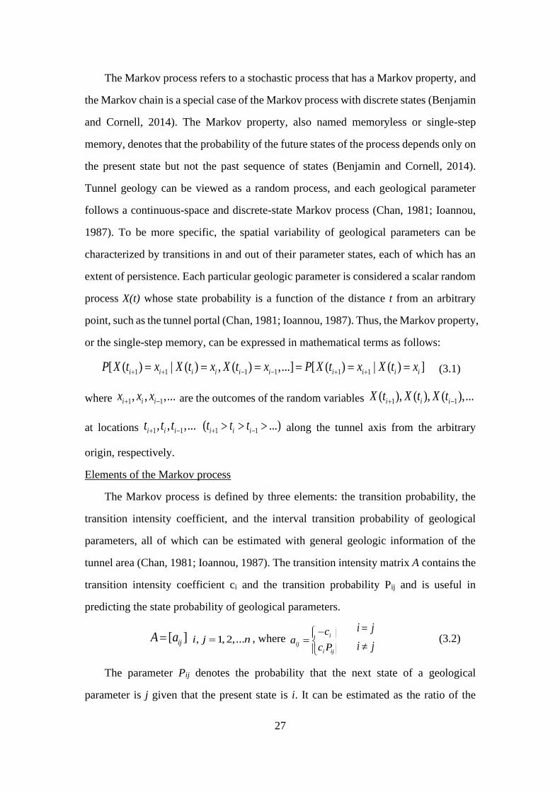
27
The Markov process refers to a stochastic process that has a Markov property, and
the Markov chain is a special case of the Markov process with discrete states (Benjamin
and Cornell, 2014). The Markov property, also named memoryless or single-step
memory, denotes that the probability of the future states of the process depends only on
the present state but not the past sequence of states (Benjamin and Cornell, 2014).
Tunnel geology can be viewed as a random process, and each geological parameter
follows a continuous-space and discrete-state Markov process (Chan, 1981; Ioannou,
1987). To be more specific, the spatial variability of geological parameters can be
characterized by transitions in and out of their parameter states, each of which has an
extent of persistence. Each particular geologic parameter is considered a scalar random
process X(t) whose state probability is a function of the distance t from an arbitrary
point, such as the tunnel portal (Chan, 1981; Ioannou, 1987). Thus, the Markov property,
or the single-step memory, can be expressed in mathematical terms as follows:
1 1 1 1 1 1[ ( ) | ( ) , ( ) ,...] [ ( ) | ( ) ]i i i i i i i i i iP X t x X t x X t x P X t x X t x+ + − − + += = = = = = (3.1)
where 1 1, , ,...i i ix x x+ − are the outcomes of the random variables 1 1( ), ( ), ( ),...i i iX t X t X t+ −
at locations 1 1, , ,...i i it t t+ − 1 1( ...)i i it t t+ − along the tunnel axis from the arbitrary
origin, respectively.
Elements of the Markov process
The Markov process is defined by three elements: the transition probability, the
transition intensity coefficient, and the interval transition probability of geological
parameters, all of which can be estimated with general geologic information of the
tunnel area (Chan, 1981; Ioannou, 1987). The transition intensity matrix A contains the
transition intensity coefficient ci and the transition probability Pij and is useful in
predicting the state probability of geological parameters.
[ ]ijA a= , 1,2,...i j n= , where i
ij
i ij
ca
c P
− =
i j
i j
=
(3.2)
The parameter Pij denotes the probability that the next state of a geological
parameter is j given that the present state is i. It can be estimated as the ratio of the
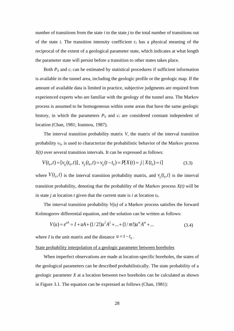
28
number of transitions from the state i to the state j to the total number of transitions out
of the state i. The transition intensity coefficient ci has a physical meaning of the
reciprocal of the extent of a geological parameter state, which indicates at what length
the parameter state will persist before a transition to other states takes place.
Both Pij and ci can be estimated by statistical procedures if sufficient information
is available in the tunnel area, including the geologic profile or the geologic map. If the
amount of available data is limited in practice, subjective judgments are required from
experienced experts who are familiar with the geology of the tunnel area. The Markov
process is assumed to be homogeneous within some areas that have the same geologic
history, in which the parameters Pij and ci are considered constant independent of
location (Chan, 1981; Ioannou, 1987).
The interval transition probability matrix V, the matrix of the interval transition
probability vij, is used to characterize the probabilistic behavior of the Markov process
X(t) over several transition intervals. It can be expressed as follows:
0 0( , ) [ ( , )]ijV t t v t t= , 0 0 0( , ) ( ) [ ( ) | ( ) ]ij ijv t t v t t P X t j X t i= − = = = (3.3)
where 0( , )V t t is the interval transition probability matrix, and 0( , )ijv t t is the interval
transition probability, denoting that the probability of the Markov process X(t) will be
in state j at location t given that the current state is i at location t0.
The interval transition probability V(u) of a Markov process satisfies the forward
Kolmogorov differential equation, and the solution can be written as follows:
2 2( ) (1/ 2!) ... (1/ !) ...uA m mV u e I uA u A m u A= = + + + + + (3.4)
where I is the unit matrix and the distance 0u t t= − .
State probability interpolation of a geologic parameter between boreholes
When imperfect observations are made at location-specific boreholes, the states of
the geological parameters can be described probabilistically. The state probability of a
geologic parameter X at a location between two boreholes can be calculated as shown
in Figure 3.1. The equation can be expressed as follows (Chan, 1981):
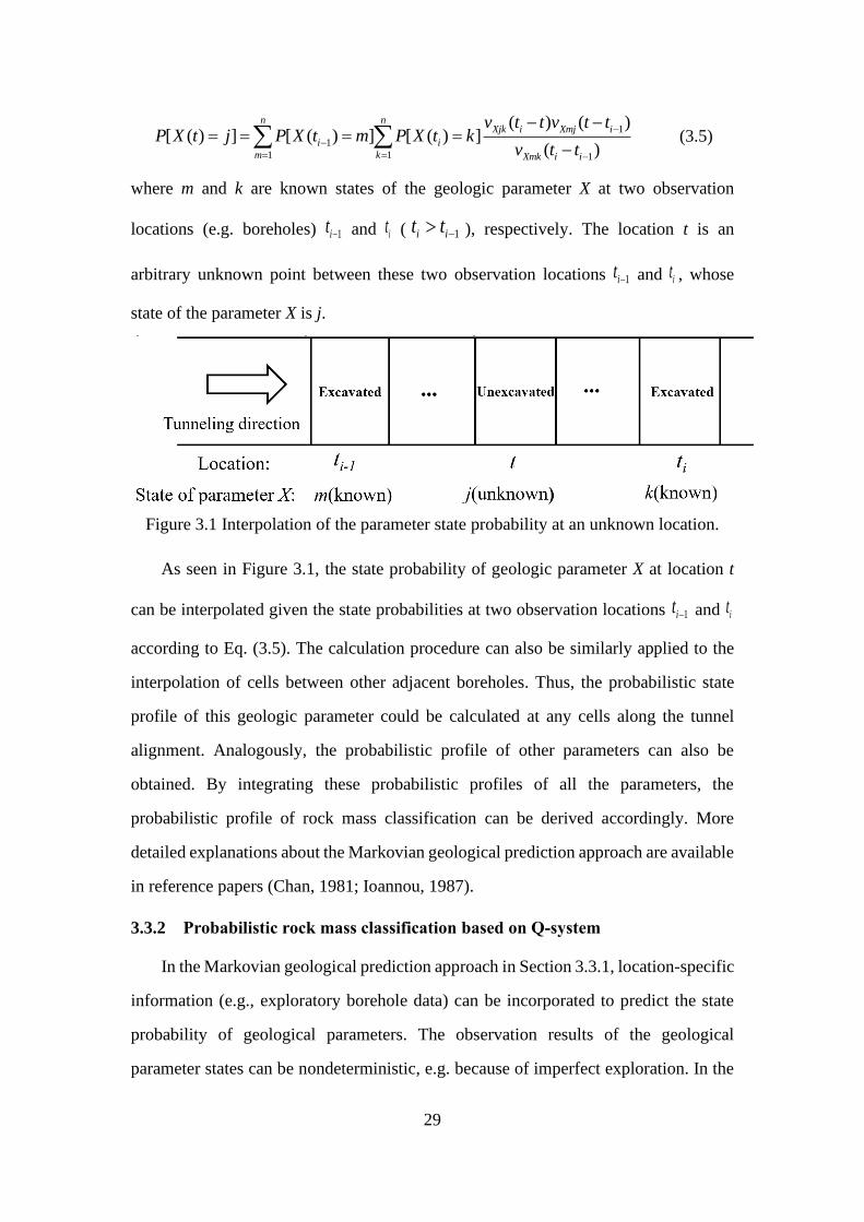
29
1
1
1 1 1
( ) ( )[ ( ) ] [ ( ) ] [ ( ) ]
( )
n nXjk i Xmj i
i i
m k Xmk i i
v t t v t tP X t j P X t m P X t k
v t t
−
−
= = −
− −= = = =
− (3.5)
where m and k are known states of the geologic parameter X at two observation
locations (e.g. boreholes) 1it − and it ( 1i it t − ), respectively. The location t is an
arbitrary unknown point between these two observation locations 1it − and it , whose
state of the parameter X is j.
Figure 3.1 Interpolation of the parameter state probability at an unknown location.
As seen in Figure 3.1, the state probability of geologic parameter X at location t
can be interpolated given the state probabilities at two observation locations 1it − and it
according to Eq. (3.5). The calculation procedure can also be similarly applied to the
interpolation of cells between other adjacent boreholes. Thus, the probabilistic state
profile of this geologic parameter could be calculated at any cells along the tunnel
alignment. Analogously, the probabilistic profile of other parameters can also be
obtained. By integrating these probabilistic profiles of all the parameters, the
probabilistic profile of rock mass classification can be derived accordingly. More
detailed explanations about the Markovian geological prediction approach are available
in reference papers (Chan, 1981; Ioannou, 1987).
3.3.2 Probabilistic rock mass classification based on Q-system
In the Markovian geological prediction approach in Section 3.3.1, location-specific
information (e.g., exploratory borehole data) can be incorporated to predict the state
probability of geological parameters. The observation results of the geological
parameter states can be nondeterministic, e.g. because of imperfect exploration. In the
30
Q-system, the likelihood matrix of Q-parameters using a particular exploration method
(e.g., subsurface borehole and face logging) at a certain location can be defined as:
( ) [ ( )];jk b jk bL t l t= ( ) [ ( ) | ( ) ]jk b b bl t P Y t k X t j= = = (3.6)
where Y(tb) is the observation result of a Q-parameter state at location tb; X(tb) is the
true state of a Q-parameter at location tb; ( )jk bl t is the likelihood (or reliability) of the
observation result k given that the true state of a Q-parameter is j at location tb, and
( )jk bL t is the likelihood matrix of a Q-parameter at location tb.
The likelihood matrix of each Q-parameter is estimated by on-site engineering
geologists, which relies on the reliability of the exploration data or the experts’
judgment. In practice, the likelihood matrix can vary due to the particular combination
of exploration methods and geologic parameters. The likelihood matrix is also a
function of location; however, for the purpose of simplicity, it is often assumed to be
constant.
3.3.3 Implementation procedures of the proposed model
The implementation procedures of the proposed model can be described as follows:
(1) Adapt state definitions, descriptions and ratings of Q-parameters to an individual
project.
The state definitions, descriptions and ratings of the Q-parameters have been
modified from Barton (2002) to individual project characteristics to establish transition
matrices of input parameters, as shown in Appendix A. For example, in cases where
squeezing and swelling are not expected to occur, SRF states characterizing these two
categorical features might not be included in the transition matrix for the parameter
SRF.
(2) Estimate the transition probability Pij and transition intensity coefficient ci.
The transition probability Pij and transition intensity coefficient ci of each Q-
parameter state are used to construct the transition matrix, which was the input for the
Markovian prediction model. These parameters could be determined by the statistical
frequency calculation if sufficient geologic data is available in the project area, by
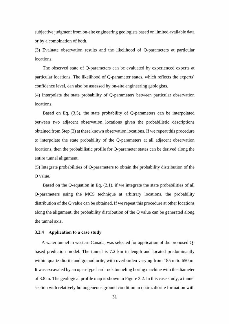
31
subjective judgment from on-site engineering geologists based on limited available data
or by a combination of both.
(3) Evaluate observation results and the likelihood of Q-parameters at particular
locations.
The observed state of Q-parameters can be evaluated by experienced experts at
particular locations. The likelihood of Q-parameter states, which reflects the experts’
confidence level, can also be assessed by on-site engineering geologists.
(4) Interpolate the state probability of Q-parameters between particular observation
locations.
Based on Eq. (3.5), the state probability of Q-parameters can be interpolated
between two adjacent observation locations given the probabilistic descriptions
obtained from Step (3) at these known observation locations. If we repeat this procedure
to interpolate the state probability of the Q-parameters at all adjacent observation
locations, then the probabilistic profile for Q-parameter states can be derived along the
entire tunnel alignment.
(5) Integrate probabilities of Q-parameters to obtain the probability distribution of the
Q value.
Based on the Q-equation in Eq. (2.1), if we integrate the state probabilities of all
Q-parameters using the MCS technique at arbitrary locations, the probability
distribution of the Q value can be obtained. If we repeat this procedure at other locations
along the alignment, the probability distribution of the Q value can be generated along
the tunnel axis.
3.3.4 Application to a case study
A water tunnel in western Canada, was selected for application of the proposed Q-
based prediction model. The tunnel is 7.2 km in length and located predominantly
within quartz diorite and granodiorite, with overburden varying from 185 m to 650 m.
It was excavated by an open-type hard rock tunneling boring machine with the diameter
of 3.8 m. The geological profile map is shown in Figure 3.2. In this case study, a tunnel
section with relatively homogeneous ground condition in quartz diorite formation with
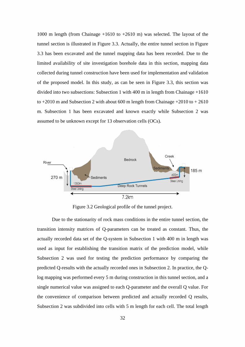
32
1000 m length (from Chainage +1610 to +2610 m) was selected. The layout of the
tunnel section is illustrated in Figure 3.3. Actually, the entire tunnel section in Figure
3.3 has been excavated and the tunnel mapping data has been recorded. Due to the
limited availability of site investigation borehole data in this section, mapping data
collected during tunnel construction have been used for implementation and validation
of the proposed model. In this study, as can be seen in Figure 3.3, this section was
divided into two subsections: Subsection 1 with 400 m in length from Chainage +1610
to +2010 m and Subsection 2 with about 600 m length from Chainage +2010 to + 2610
m. Subsection 1 has been excavated and known exactly while Subsection 2 was
assumed to be unknown except for 13 observation cells (OCs).
Figure 3.2 Geological profile of the tunnel project.
Due to the stationarity of rock mass conditions in the entire tunnel section, the
transition intensity matrices of Q-parameters can be treated as constant. Thus, the
actually recorded data set of the Q-system in Subsection 1 with 400 m in length was
used as input for establishing the transition matrix of the prediction model, while
Subsection 2 was used for testing the prediction performance by comparing the
predicted Q-results with the actually recorded ones in Subsection 2. In practice, the Q-
log mapping was performed every 5 m during construction in this tunnel section, and a
single numerical value was assigned to each Q-parameter and the overall Q value. For
the convenience of comparison between predicted and actually recorded Q results,
Subsection 2 was subdivided into cells with 5 m length for each cell. The total length
33
of Subsection 2 is 605 m and thus 121 cells are obtained with 13 OCs. The OC 1 is at
Chainage +2010~2015 m, which is the starting cell in Subsection 2. This cell was
considered as the reference starting point for the subsequent prediction. In other words,
OC 1 is the starting Cell 1 while OC 13 is Cell 61 in Subsection 2.
To investigate the effects of the input data, i.e. Q data in Subsection 1, on the
prediction performance, two additional scenarios, including the Subsection 1 with 200
m (Chainage +1610~1810 m) and 300 m (Chainage +1610~1910 m), have also been
conducted. The Subsection 2 with 600 m (Chainage +2010~2610) is used as the test
subsection to verify the prediction performance with input data obtained from
Subsection 1 with different length (200 m, 300 m and 400 m). The following section in
this chapter focuses on the results derived from the scenario with Subsection 1 of 400
m. The main results for the other two scenarios with Subsection 1 of 200 m and 300 m
are listed in Appendix D.
Figure 3.3 Layout of observation cells in this tunnel section.
3.4 Results and discussion
3.4.1 Probabilistic profiles of Q-system
Probabilistic Profile of States of Q-parameters
The state definitions, descriptions and ratings for Q-parameters in this case
study are shown in Appendix A. Note that SRF states for squeezing and swelling rocks
are not included in Appendix A since these scenarios are not expected to be encountered
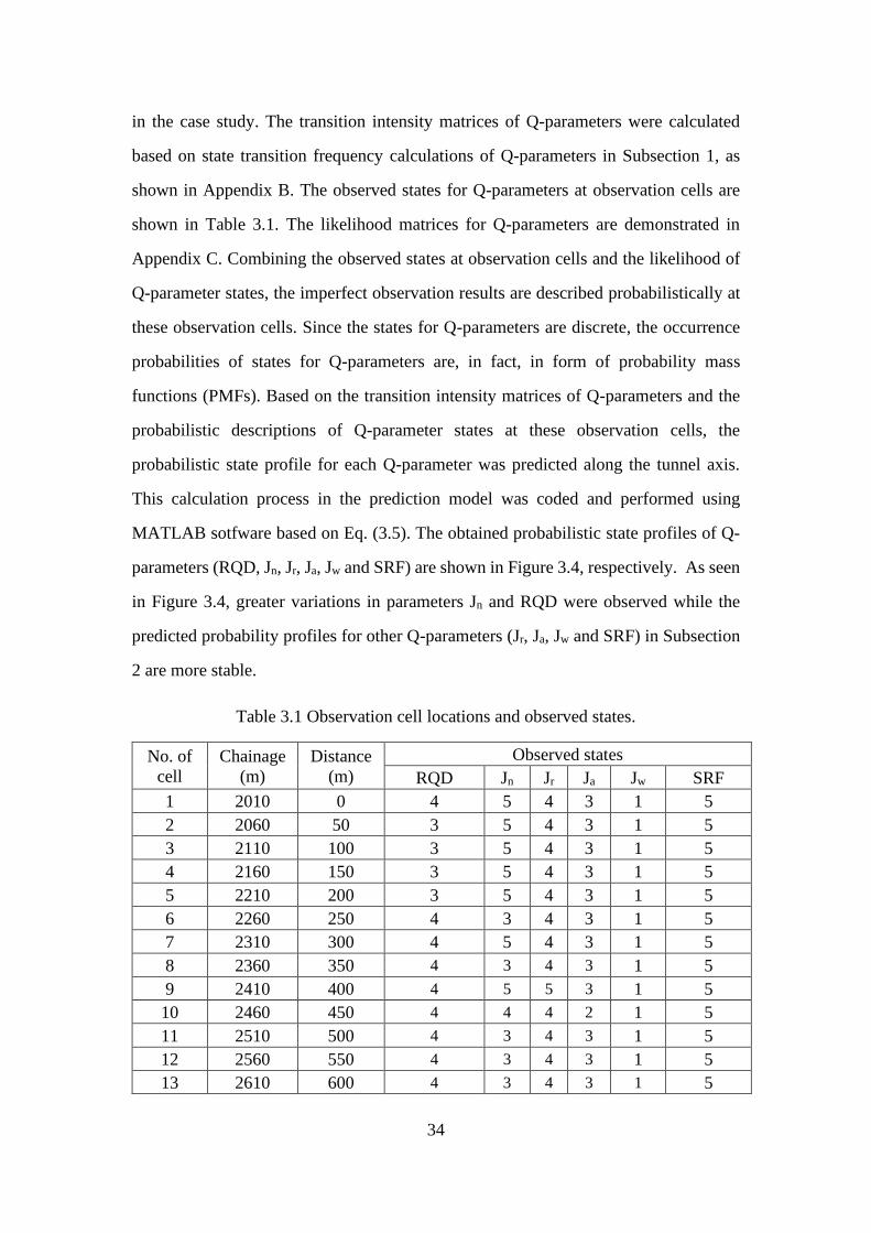
34
in the case study. The transition intensity matrices of Q-parameters were calculated
based on state transition frequency calculations of Q-parameters in Subsection 1, as
shown in Appendix B. The observed states for Q-parameters at observation cells are
shown in Table 3.1. The likelihood matrices for Q-parameters are demonstrated in
Appendix C. Combining the observed states at observation cells and the likelihood of
Q-parameter states, the imperfect observation results are described probabilistically at
these observation cells. Since the states for Q-parameters are discrete, the occurrence
probabilities of states for Q-parameters are, in fact, in form of probability mass
functions (PMFs). Based on the transition intensity matrices of Q-parameters and the
probabilistic descriptions of Q-parameter states at these observation cells, the
probabilistic state profile for each Q-parameter was predicted along the tunnel axis.
This calculation process in the prediction model was coded and performed using
MATLAB sotfware based on Eq. (3.5). The obtained probabilistic state profiles of Q-
parameters (RQD, Jn, Jr, Ja, Jw and SRF) are shown in Figure 3.4, respectively. As seen
in Figure 3.4, greater variations in parameters Jn and RQD were observed while the
predicted probability profiles for other Q-parameters (Jr, Ja, Jw and SRF) in Subsection
2 are more stable.
Table 3.1 Observation cell locations and observed states.
No. of
cell
Chainage
(m)
Distance
(m)
Observed states
RQD Jn Jr Ja Jw SRF
1 2010 0 4 5 4 3 1 5
2 2060 50 3 5 4 3 1 5
3 2110 100 3 5 4 3 1 5
4 2160 150 3 5 4 3 1 5
5 2210 200 3 5 4 3 1 5
6 2260 250 4 3 4 3 1 5
7 2310 300 4 5 4 3 1 5
8 2360 350 4 3 4 3 1 5
9 2410 400 4 5 5 3 1 5
10 2460 450 4 4 4 2 1 5
11 2510 500 4 3 4 3 1 5
12 2560 550 4 3 4 3 1 5
13 2610 600 4 3 4 3 1 5
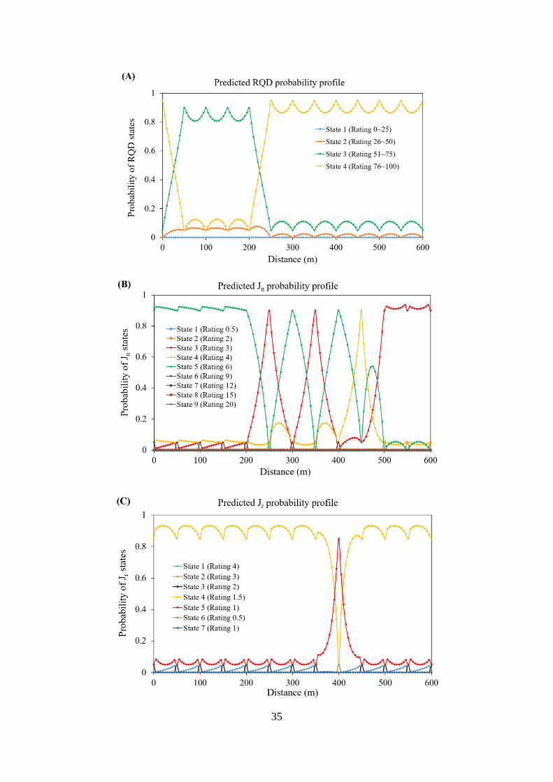
35
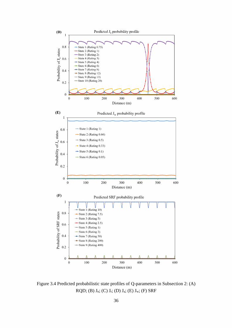
36
Figure 3.4 Predicted probabilistic state profiles of Q-parameters in Subsection 2: (A)
RQD; (B) Jn; (C) Jr; (D) Ja; (E) Jw; (F) SRF
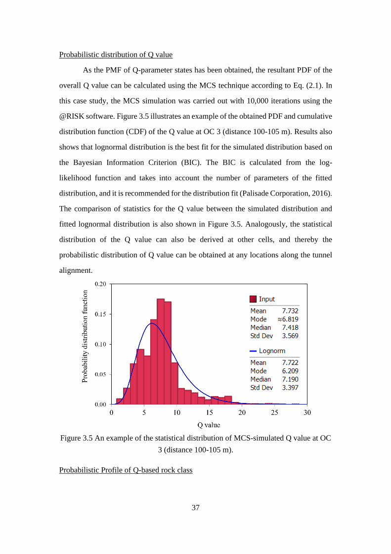
37
Probabilistic distribution of Q value
As the PMF of Q-parameter states has been obtained, the resultant PDF of the
overall Q value can be calculated using the MCS technique according to Eq. (2.1). In
this case study, the MCS simulation was carried out with 10,000 iterations using the
@RISK software. Figure 3.5 illustrates an example of the obtained PDF and cumulative
distribution function (CDF) of the Q value at OC 3 (distance 100-105 m). Results also
shows that lognormal distribution is the best fit for the simulated distribution based on
the Bayesian Information Criterion (BIC). The BIC is calculated from the log-
likelihood function and takes into account the number of parameters of the fitted
distribution, and it is recommended for the distribution fit (Palisade Corporation, 2016).
The comparison of statistics for the Q value between the simulated distribution and
fitted lognormal distribution is also shown in Figure 3.5. Analogously, the statistical
distribution of the Q value can also be derived at other cells, and thereby the
probabilistic distribution of Q value can be obtained at any locations along the tunnel
alignment.
Figure 3.5 An example of the statistical distribution of MCS-simulated Q value at OC
3 (distance 100-105 m).
Probabilistic Profile of Q-based rock class
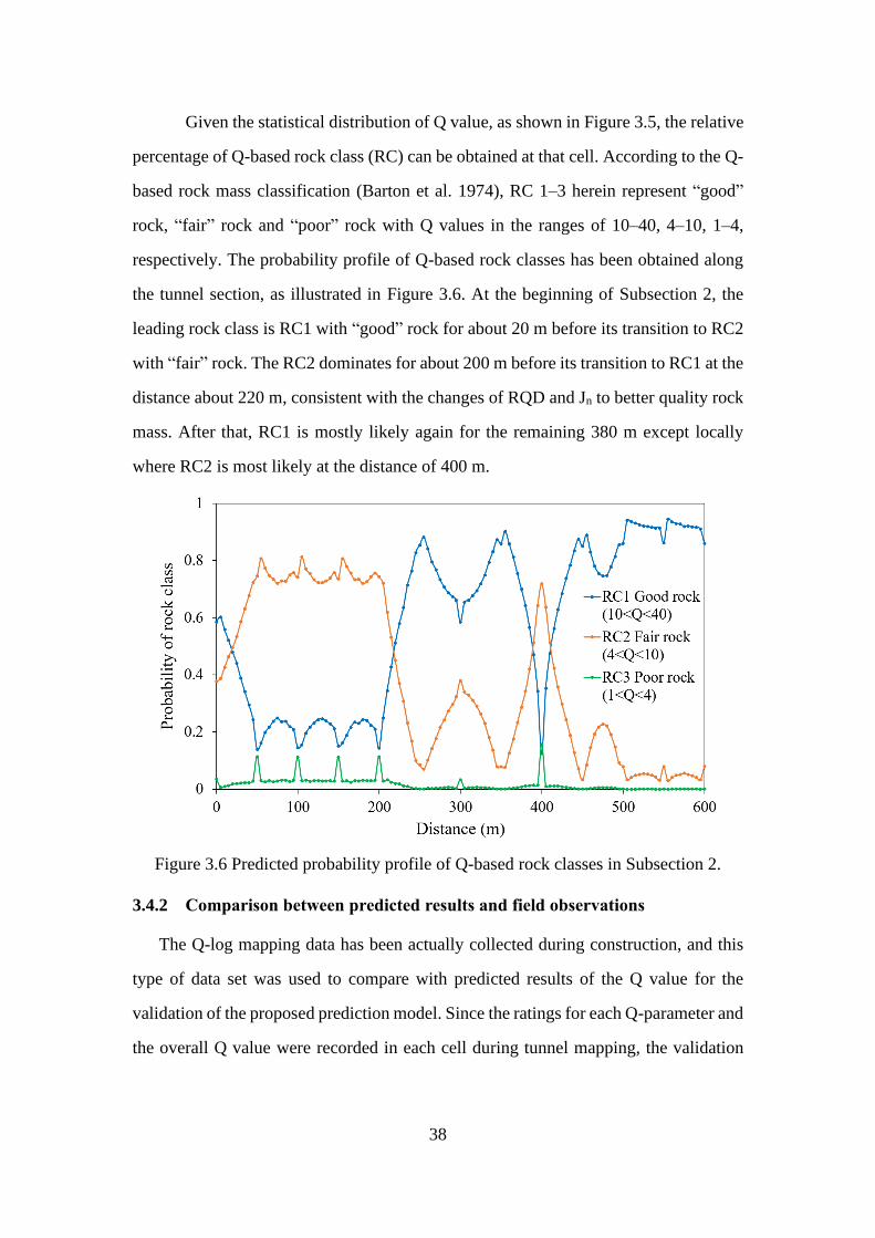
38
Given the statistical distribution of Q value, as shown in Figure 3.5, the relative
percentage of Q-based rock class (RC) can be obtained at that cell. According to the Q-
based rock mass classification (Barton et al. 1974), RC 1–3 herein represent “good”
rock, “fair” rock and “poor” rock with Q values in the ranges of 10–40, 4–10, 1–4,
respectively. The probability profile of Q-based rock classes has been obtained along
the tunnel section, as illustrated in Figure 3.6. At the beginning of Subsection 2, the
leading rock class is RC1 with “good” rock for about 20 m before its transition to RC2
with “fair” rock. The RC2 dominates for about 200 m before its transition to RC1 at the
distance about 220 m, consistent with the changes of RQD and Jn to better quality rock
mass. After that, RC1 is mostly likely again for the remaining 380 m except locally
where RC2 is most likely at the distance of 400 m.
Figure 3.6 Predicted probability profile of Q-based rock classes in Subsection 2.
3.4.2 Comparison between predicted results and field observations
The Q-log mapping data has been actually collected during construction, and this
type of data set was used to compare with predicted results of the Q value for the
validation of the proposed prediction model. Since the ratings for each Q-parameter and
the overall Q value were recorded in each cell during tunnel mapping, the validation

39
can be performed by comparing predicted Q-parameter states, Q values and Q-based
rock classes with those actually collected during tunnel construction.
Comparison criterion of Q-parameter states
To test predicted results of Q-parameter states, the accuracy plot has been used.
In the accuracy plot for predicted Q-parameter states, the horizontal axis indicates the
probability interval of predicted mostly likely outcome for each Q-parameter, which
can be obtained in Figure 3.4. The vertical axis means the proportion of the actually
recorded results in this interval in all cells of the Subsection 2. A perfect prediction
corresponds to the 1:1 line in the accuracy plot. Figure 3.7 and Figure 3.8 illustrate the
accuracy plots for the predicted RQD and Jn in Subsection 2, respectively. The
probability interval is in unit of 10% in this case. Take the accuracy plot of RQD as an
example, in the interval of 0.8~0.9, the middle value of 0.85 is used. The number of
cells in which the predicted modal probabilities are in this interval of 0.8~0.9 is 79 in
Subsection, as obtained in the predicted probability profile of RQD in Figure 3.4. Based
on the actually recorded RQD states in Subsection 2, there are 66 out of 79 cells where
the predicted modal outcomes correspond to the actually mapped states, giving the
proportion of true states about 84% in this interval of 0.8~0.9. The calculated proportion
value in certain probability interval reflects the actual prediction correctness in this
probability interval. Similarly, the proportion values in other probability intervals for
the predicted RQD and for other Q-parameters were also derived and the accuracy plots
have been obtained for Q-parameters.
The measures of prediction accuracy, including the RMSE (Root Mean Square
Error) and R2 (coefficient of determination), have also been derived in the accuracy
plots. It can be seen in Figure 3.7 and Figure 3.8 that R2 values for both predicted RQD
and Jn are above 0.8 and RMSE values are around 0.1, indicating the relatively good
prediction performance. As can be seen in Figure 3.4, there are greater variations in the
predicted probability profiles for RQD and Jn while a certain state is dominant in the
majority of Subsection 2 for other Q-parameters (Jr, Ja, Jw and SRF). Actually recorded
results also reveal that the mapped state results for RQD and Jn are more variable than
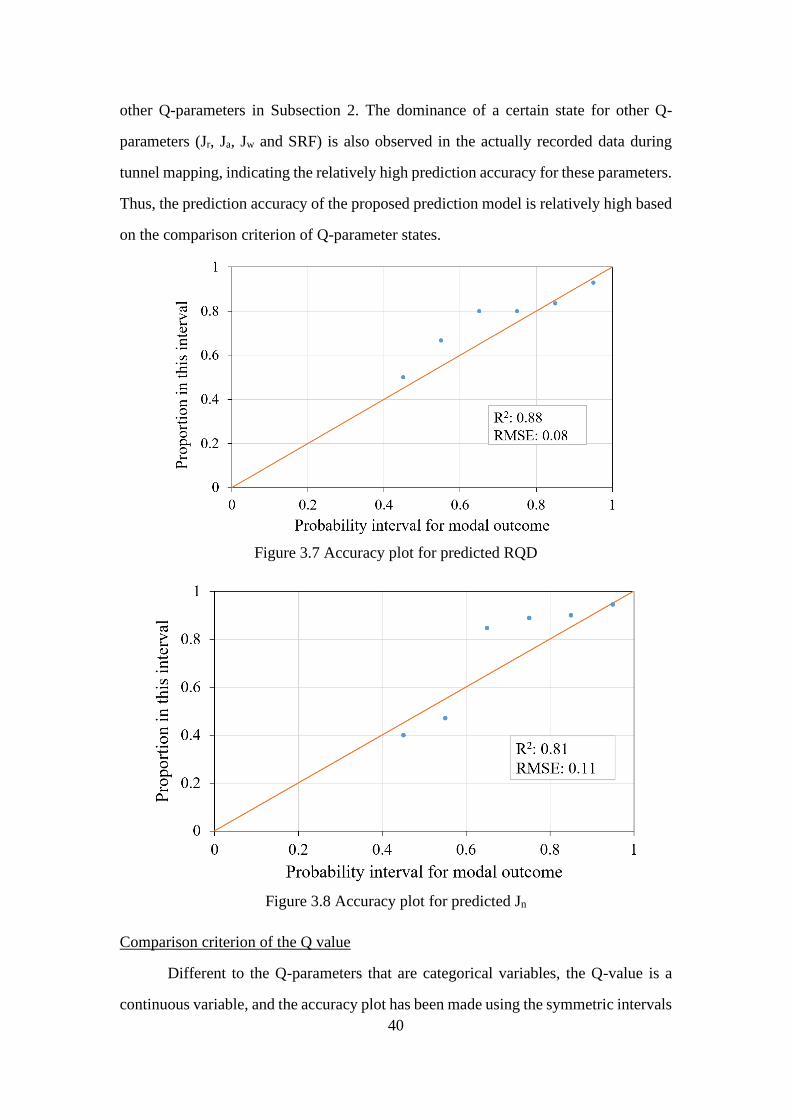
40
other Q-parameters in Subsection 2. The dominance of a certain state for other Q-
parameters (Jr, Ja, Jw and SRF) is also observed in the actually recorded data during
tunnel mapping, indicating the relatively high prediction accuracy for these parameters.
Thus, the prediction accuracy of the proposed prediction model is relatively high based
on the comparison criterion of Q-parameter states.
Figure 3.7 Accuracy plot for predicted RQD
Figure 3.8 Accuracy plot for predicted Jn
Comparison criterion of the Q value
Different to the Q-parameters that are categorical variables, the Q-value is a
continuous variable, and the accuracy plot has been made using the symmetric intervals
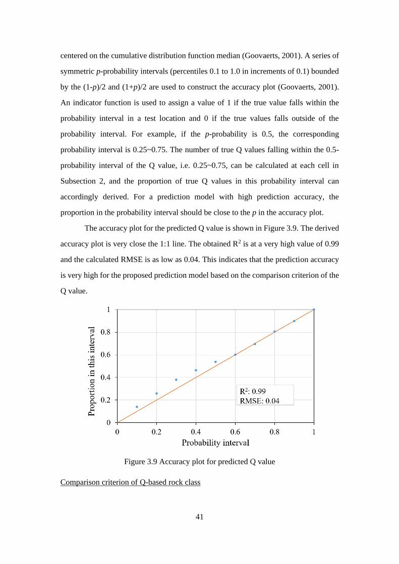
41
centered on the cumulative distribution function median (Goovaerts, 2001). A series of
symmetric p-probability intervals (percentiles 0.1 to 1.0 in increments of 0.1) bounded
by the (1-p)/2 and (1+p)/2 are used to construct the accuracy plot (Goovaerts, 2001).
An indicator function is used to assign a value of 1 if the true value falls within the
probability interval in a test location and 0 if the true values falls outside of the
probability interval. For example, if the p-probability is 0.5, the corresponding
probability interval is 0.25~0.75. The number of true Q values falling within the 0.5-
probability interval of the Q value, i.e. 0.25~0.75, can be calculated at each cell in
Subsection 2, and the proportion of true Q values in this probability interval can
accordingly derived. For a prediction model with high prediction accuracy, the
proportion in the probability interval should be close to the p in the accuracy plot.
The accuracy plot for the predicted Q value is shown in Figure 3.9. The derived
accuracy plot is very close the 1:1 line. The obtained R2 is at a very high value of 0.99
and the calculated RMSE is as low as 0.04. This indicates that the prediction accuracy
is very high for the proposed prediction model based on the comparison criterion of the
Q value.
Figure 3.9 Accuracy plot for predicted Q value
Comparison criterion of Q-based rock class
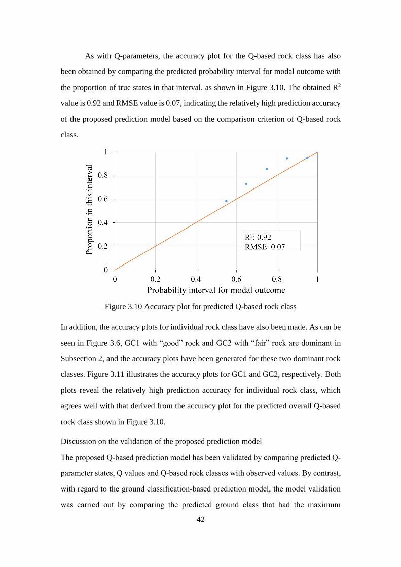
42
As with Q-parameters, the accuracy plot for the Q-based rock class has also
been obtained by comparing the predicted probability interval for modal outcome with
the proportion of true states in that interval, as shown in Figure 3.10. The obtained R2
value is 0.92 and RMSE value is 0.07, indicating the relatively high prediction accuracy
of the proposed prediction model based on the comparison criterion of Q-based rock
class.
Figure 3.10 Accuracy plot for predicted Q-based rock class
In addition, the accuracy plots for individual rock class have also been made. As can be
seen in Figure 3.6, GC1 with “good” rock and GC2 with “fair” rock are dominant in
Subsection 2, and the accuracy plots have been generated for these two dominant rock
classes. Figure 3.11 illustrates the accuracy plots for GC1 and GC2, respectively. Both
plots reveal the relatively high prediction accuracy for individual rock class, which
agrees well with that derived from the accuracy plot for the predicted overall Q-based
rock class shown in Figure 3.10.
Discussion on the validation of the proposed prediction model
The proposed Q-based prediction model has been validated by comparing predicted Q-
parameter states, Q values and Q-based rock classes with observed values. By contrast,
with regard to the ground classification-based prediction model, the model validation
was carried out by comparing the predicted ground class that had the maximum
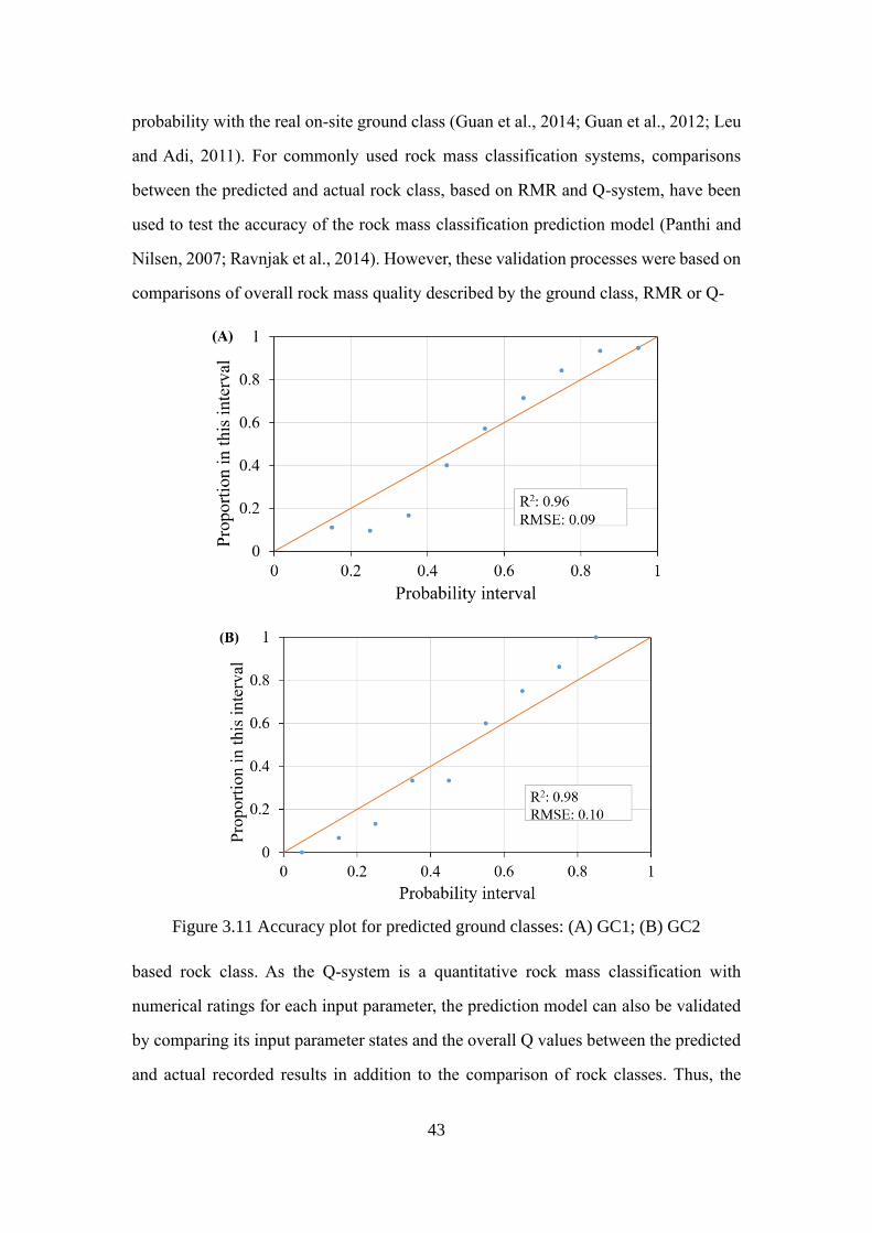
43
probability with the real on-site ground class (Guan et al., 2014; Guan et al., 2012; Leu
and Adi, 2011). For commonly used rock mass classification systems, comparisons
between the predicted and actual rock class, based on RMR and Q-system, have been
used to test the accuracy of the rock mass classification prediction model (Panthi and
Nilsen, 2007; Ravnjak et al., 2014). However, these validation processes were based on
comparisons of overall rock mass quality described by the ground class, RMR or Q-
Figure 3.11 Accuracy plot for predicted ground classes: (A) GC1; (B) GC2
based rock class. As the Q-system is a quantitative rock mass classification with
numerical ratings for each input parameter, the prediction model can also be validated
by comparing its input parameter states and the overall Q values between the predicted
and actual recorded results in addition to the comparison of rock classes. Thus, the
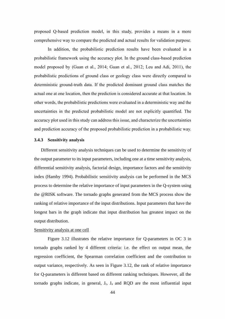
44
proposed Q-based prediction model, in this study, provides a means in a more
comprehensive way to compare the predicted and actual results for validation purpose.
In addition, the probabilistic prediction results have been evaluated in a
probabilistic framework using the accuracy plot. In the ground class-based prediction
model proposed by (Guan et al., 2014; Guan et al., 2012; Leu and Adi, 2011), the
probabilistic predictions of ground class or geology class were directly compared to
deterministic ground-truth data. If the predicted dominant ground class matches the
actual one at one location, then the prediction is considered accurate at that location. In
other words, the probabilistic predictions were evaluated in a deterministic way and the
uncertainties in the predicted probabilistic model are not explicitly quantified. The
accuracy plot used in this study can address this issue, and characterize the uncertainties
and prediction accuracy of the proposed probabilistic prediction in a probabilistic way.
3.4.3 Sensitivity analysis
Different sensitivity analysis techniques can be used to determine the sensitivity of
the output parameter to its input parameters, including one at a time sensitivity analysis,
differential sensitivity analysis, factorial design, importance factors and the sensitivity
index (Hamby 1994). Probabilistic sensitivity analysis can be performed in the MCS
process to determine the relative importance of input parameters in the Q-system using
the @RISK software. The tornado graphs generated from the MCS process show the
ranking of relative importance of the input distributions. Input parameters that have the
longest bars in the graph indicate that input distribution has greatest impact on the
output distribution.
Sensitivity analysis at one cell
Figure 3.12 illustrates the relative importance for Q-parameters in OC 3 in
tornado graphs ranked by 4 different criteria: i.e. the effect on output mean, the
regression coefficient, the Spearman correlation coefficient and the contribution to
output variance, respectively. As seen in Figure 3.12, the rank of relative importance
for Q-parameters is different based on different ranking techniques. However, all the
tornado graphs indicate, in general, Jr, Ja and RQD are the most influential input
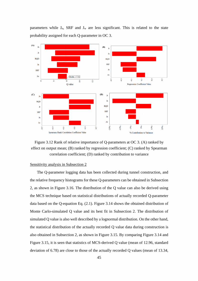
45
parameters while Jn, SRF and Jw are less significant. This is related to the state
probability assigned for each Q-parameter in OC 3.
Figure 3.12 Rank of relative importance of Q-parameters at OC 3. (A) ranked by
effect on output mean; (B) ranked by regression coefficient; (C) ranked by Spearman
correlation coefficient; (D) ranked by contribution to variance
Sensitivity analysis in Subsection 2
The Q-parameter logging data has been collected during tunnel construction, and
the relative frequency histograms for these Q-parameters can be obtained in Subsection
2, as shown in Figure 3.16. The distribution of the Q value can also be derived using
the MCS technique based on statistical distributions of actually recorded Q-parameter
data based on the Q-equation Eq. (2.1). Figure 3.14 shows the obtained distribution of
Monte Carlo-simulated Q value and its best fit in Subsection 2. The distribution of
simulated Q value is also well described by a lognormal distribution. On the other hand,
the statistical distribution of the actually recorded Q value data during construction is
also obtained in Subsection 2, as shown in Figure 3.15. By comparing Figure 3.14 and
Figure 3.15, it is seen that statistics of MCS-derived Q value (mean of 12.96, standard
deviation of 6.78) are close to those of the actually recorded Q values (mean of 13.34,
46
standard deviation of 7.10), indicating the effectiveness of the MCS technique in
characterizing uncertainty propagation from input parameters to the output. In addition,
the relative percentage of Q-based rock class was also compared for simulated and
actually recorded results, as illustrated in Figure 3.16. In general, the simulated and
actually recorded Q-based rock class results agree well with each other. It is also found
that “good” and “fair” rocks are dominant, covering more than 95% in total, for both
simulated and actually recorded Q-based rock classes. Thus, the MCS-derived rock
class percentage can also provide preliminary estimation of the overall rock mass
quality in the tunnel section before excavation.
Figure 3.13 Relative frequency histogram collected in Subsection 2: (A) RQD; (B) Jn;
(C) Jr; (D) Ja; (E) Jw; (F) SRF
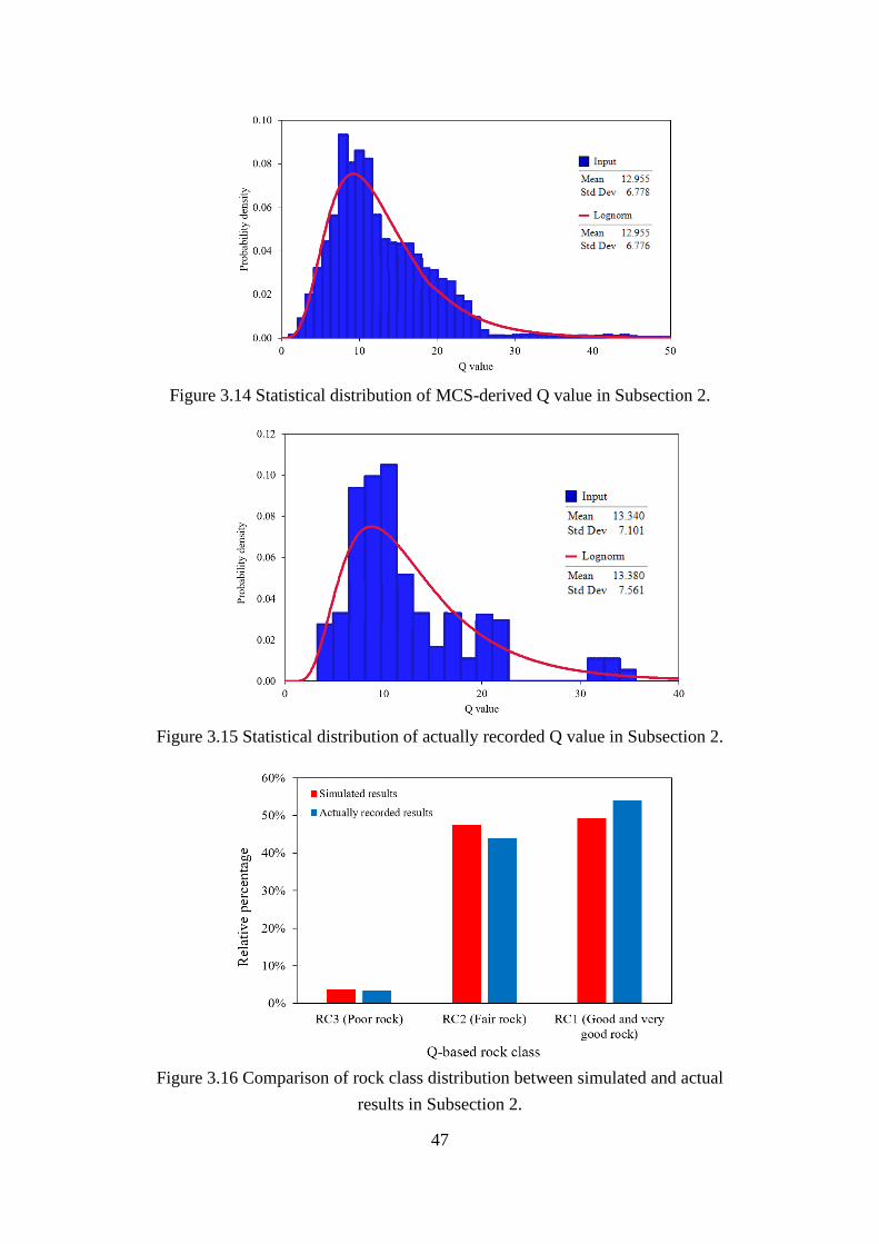
47
Figure 3.14 Statistical distribution of MCS-derived Q value in Subsection 2.
Figure 3.15 Statistical distribution of actually recorded Q value in Subsection 2.
Figure 3.16 Comparison of rock class distribution between simulated and actual
results in Subsection 2.
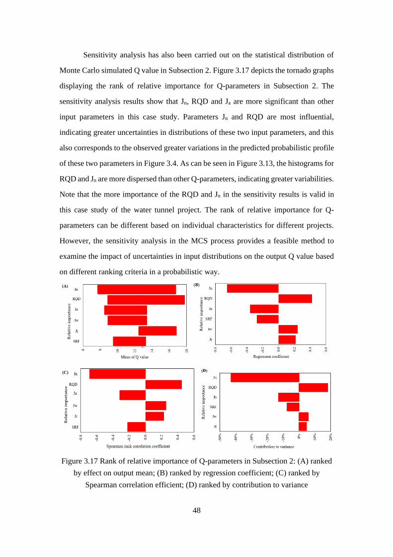
48
Sensitivity analysis has also been carried out on the statistical distribution of
Monte Carlo simulated Q value in Subsection 2. Figure 3.17 depicts the tornado graphs
displaying the rank of relative importance for Q-parameters in Subsection 2. The
sensitivity analysis results show that Jn, RQD and Ja are more significant than other
input parameters in this case study. Parameters Jn and RQD are most influential,
indicating greater uncertainties in distributions of these two input parameters, and this
also corresponds to the observed greater variations in the predicted probabilistic profile
of these two parameters in Figure 3.4. As can be seen in Figure 3.13, the histograms for
RQD and Jn are more dispersed than other Q-parameters, indicating greater variabilities.
Note that the more importance of the RQD and Jn in the sensitivity results is valid in
this case study of the water tunnel project. The rank of relative importance for Q-
parameters can be different based on individual characteristics for different projects.
However, the sensitivity analysis in the MCS process provides a feasible method to
examine the impact of uncertainties in input distributions on the output Q value based
on different ranking criteria in a probabilistic way.
Figure 3.17 Rank of relative importance of Q-parameters in Subsection 2: (A) ranked
by effect on output mean; (B) ranked by regression coefficient; (C) ranked by
Spearman correlation efficient; (D) ranked by contribution to variance

49
3.4.4 Analytical calculation approach to deriving statistics of Q value
Analytical approximation on statistics of Q value
The statistics of a product of several input parameters, including the mean,
standard deviation and coefficient of variation (COV), can be approximated using
Taylor expansions given those statistics of input parameters (Elandt-Johnson and
Johnson, 1980). Since the Q value is the product of three quotients as shown in the Q-
equation in Eq. (2.1), statistics of the Q value can be accordingly calculated given
statistics of Q-parameters. In this section, an analytical approximate calculation
approach to deriving statistics of the Q value is proposed accounting for the
uncertainties in Q-parameters, and the derivation procedures are shown in Appendix E
in detail. It should be noted that for the derivation COV of Q value, it can either be
calculated as the ratio of standard deviation to the mean of obtained Q value by
definition, or derived through the COV of Q-parameters. For the simplicity of
calculation, all the Q-parameters are assumed to be independent in this derivation
process.
Comparison between analytical and simulated Q value
The relative frequency histogram for each Q-parameter has been obtained at
each cell in the tunnel section, and statistics for each Q-parameter has also been
obtained using the @RISK software. Given the statistics of Q-parameters, the statistics
of the Q value can be approximated using the developed analytical calculation approach.
Table 3.2 compares statistics of the Q value among analytical, Monte Carlo-simulated
and actually recorded results in OC 3 and Subsection 2, respectively. The Q-equation
approach in the analytical solution is also included, in which the mean of Q value was
calculated directly based on the Q-equation in Eq. (2.1) with the mean of each Q-
parameter as the only input. In this Q-equation approach, only the mean value rather
than the standard deviation and COV of the Q value is calculated since the dispersion
(e.g. SD and COV) of Q-parameters is not considered. In contrast, in the proposed
calculation approach, the standard deviation and COV of Q-parameters are taken into
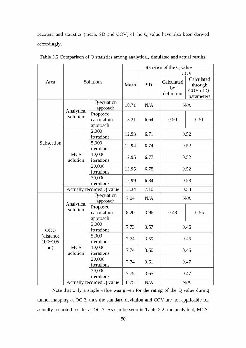
50
account, and statistics (mean, SD and COV) of the Q value have also been derived
accordingly.
Table 3.2 Comparison of Q statistics among analytical, simulated and actual results.
Area Solutions
Statistics of the Q value
Mean SD
COV
Calculated
by
definition
Calculated
through
COV of Q-
parameters
Subsection
2
Analytical
solution
Q-equation
approach 10.71 N/A N/A
Proposed
calculation
approach
13.21 6.64 0.50 0.51
MCS
solution
2,000
iterations 12.93 6.71 0.52
5,000
iterations 12.94 6.74 0.52
10,000
iterations 12.95 6.77 0.52
20,000
iterations 12.95 6.78 0.52
30,000
iterations 12.99 6.84 0.53
Actually recorded Q value 13.34 7.10 0.53
OC 3
(distance
100~105
m)
Analytical
solution
Q-equation
approach 7.04 N/A N/A
Proposed
calculation
approach
8.20 3.96 0.48 0.55
MCS
solution
3,000
iterations 7.73 3.57 0.46
5,000
iterations 7.74 3.59 0.46
10,000
iterations 7.74 3.60 0.46
20,000
iterations 7.74 3.61 0.47
30,000
iterations 7.75 3.65 0.47
Actually recorded Q value 8.75 N/A N/A
Note that only a single value was given for the rating of the Q value during
tunnel mapping at OC 3, thus the standard deviation and COV are not applicable for
actually recorded results at OC 3. As can be seen in Table 3.2, the analytical, MCS-
51
simulated and actually recorded results in terms of the mean, standard deviation and
COV of the Q value are, in general, close in both OC 3 and Subsection 2. The generated
statistics in analytical and simulated solutions are smaller than that in actually recorded
results, but the differences are insignificant. With regard to the analytical solution, the
obtained mean value in the proposed calculation approach (13.21) is closer to the
recorded value (13.34) than that derived from the Q-equation approach (10.71) in
Subsection 2. In addition, the measure of variations (SD and COV) for the estimated Q
value can also be obtained in the proposed calculation approach, as shown in Table 3.2.
In terms of the MCS solution, it is seen that greater mean and dispersion of the Q value
are obtained with increased iterations. However, the differences are also limited,
meaning the effect of iteration runs on simulated results is insignificant in this case
study.
As mentioned above, the results derived from the proposed calculation approach
were close to MCS-simulated and actually recorded results in OC 3. This analytical
approximation procedures can also be performed at other cells in Subsection 2. The
analytical approximation process has been carried out at all cells in Subsection 2.
Figure 3.18 shows the comparison of derived mean and standard deviation of Q
values between analytical and simulated results (3,000 iterations) in Subsection 2. The
comparison of COV for Q values is illustrated in Figure 3.19. It is shown that the
analytical means of Q values are very close to those of simulated ones along the section.
Compared to the mean values, the standard deviation and COV have greater variations
between analytical and simulated results. The analytical calculation results reveal less
dispersion in the Q value than the MCS-derived results. The relative difference of
statistics of the Q value between analytical and simulated results along Subsection 2 is
demonstrated in Figure 3.20. The relative difference is calculated as the absolute
difference between the analytical and simulated Q statistics divided by the analytical
values. It is seen that the relative difference of the mean is low between the analytical
and simulated results along Subsection 2 with the maximum value around 5%. In
contrast, the relative difference values for SD and COV are higher with the majority of
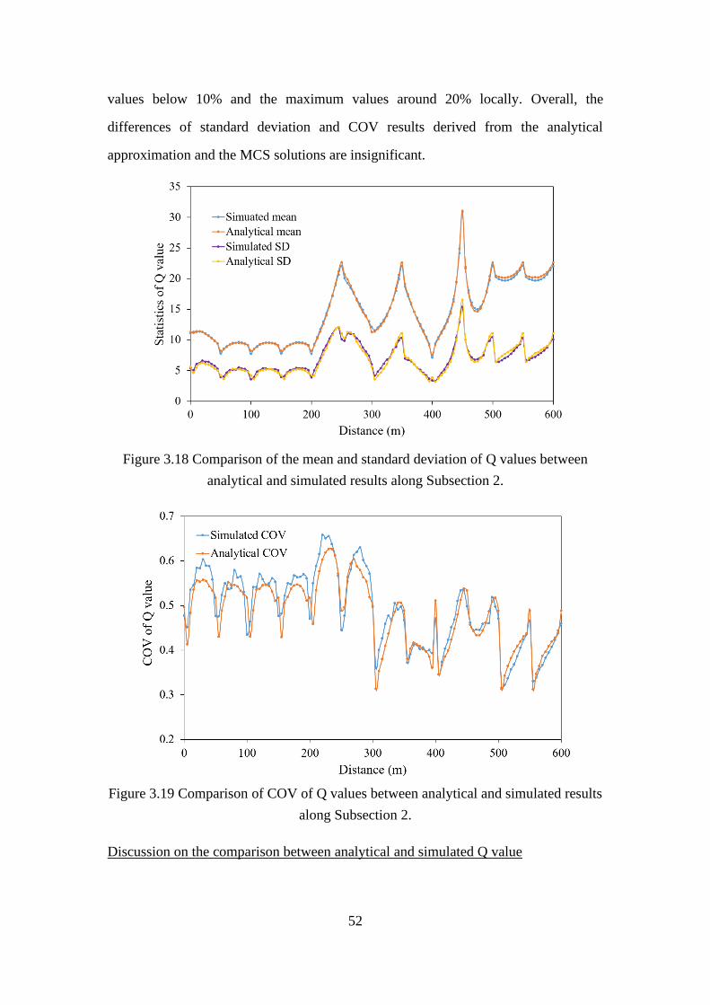
52
values below 10% and the maximum values around 20% locally. Overall, the
differences of standard deviation and COV results derived from the analytical
approximation and the MCS solutions are insignificant.
Figure 3.18 Comparison of the mean and standard deviation of Q values between
analytical and simulated results along Subsection 2.
Figure 3.19 Comparison of COV of Q values between analytical and simulated results
along Subsection 2.
Discussion on the comparison between analytical and simulated Q value
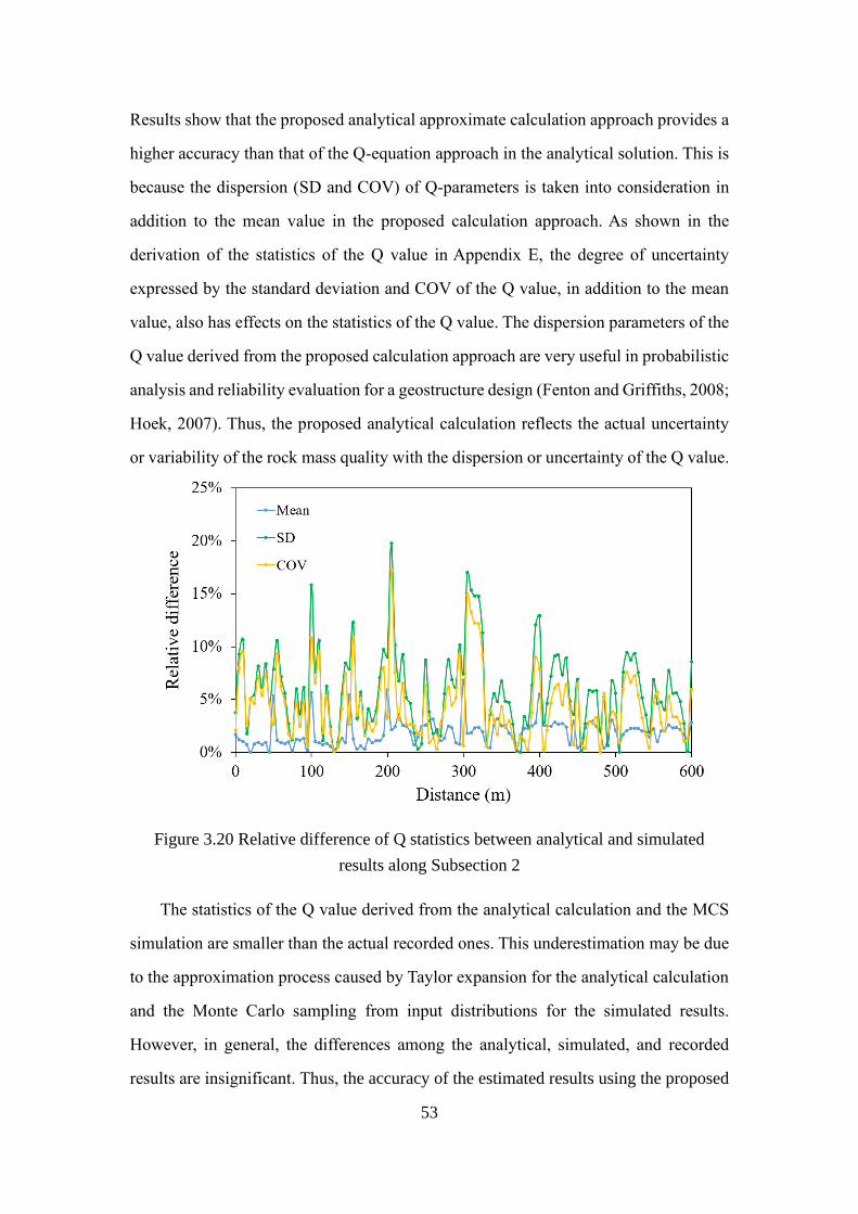
53
Results show that the proposed analytical approximate calculation approach provides a
higher accuracy than that of the Q-equation approach in the analytical solution. This is
because the dispersion (SD and COV) of Q-parameters is taken into consideration in
addition to the mean value in the proposed calculation approach. As shown in the
derivation of the statistics of the Q value in Appendix E, the degree of uncertainty
expressed by the standard deviation and COV of the Q value, in addition to the mean
value, also has effects on the statistics of the Q value. The dispersion parameters of the
Q value derived from the proposed calculation approach are very useful in probabilistic
analysis and reliability evaluation for a geostructure design (Fenton and Griffiths, 2008;
Hoek, 2007). Thus, the proposed analytical calculation reflects the actual uncertainty
or variability of the rock mass quality with the dispersion or uncertainty of the Q value.
Figure 3.20 Relative difference of Q statistics between analytical and simulated
results along Subsection 2
The statistics of the Q value derived from the analytical calculation and the MCS
simulation are smaller than the actual recorded ones. This underestimation may be due
to the approximation process caused by Taylor expansion for the analytical calculation
and the Monte Carlo sampling from input distributions for the simulated results.
However, in general, the differences among the analytical, simulated, and recorded
results are insignificant. Thus, the accuracy of the estimated results using the proposed
54
analytical calculation approach and the MCS technique has been validated by the
actually recorded Q value. The MCS technique is capable of providing a complete
probability distribution of the estimated Q value and associated statistics, and its
advantage in describing the uncertainty propagation in rock mass classifications has
also been reported in literature (Bedi, 2014; Cai, 2011; Panthi, 2006; Sari, 2009; Sari et
al., 2010). Thus, the MCS technique can be helpful in providing good estimates of the
actual rock mass quality and associated uncertainties in the tunnel section before
construction.
3.4.5 Effects of the correlation between Q-parameters on Q value
Correlation between RQD and Jn
A correlation between RQD and volumetric joint frequency v was reported by
Palmstrom (2005), and can be described as:
110 2.5RQD v= − (4 44)v (3.7)
The volumetric joint frequency v can be expressed as (Palmstrom and Stille, 2010):
1
1( )
5
Nr
i i
Nv
s
=
= + (3.8)
where si is the mean joint set spacing in meters of the ith joint set; N is the total number
of joint sets; and Nr is the number of random joints.
It is seen that RQD is negatively correlated to the volumetric joint frequency v
from Eq. (3.7) and that v is positively correlated to the total number of joint sets N
from Eq. (3.8). Combining these two equations, it is obtained that RQD is negatively
correlated to the number of joint sets N, which is consistent with the rating of Jn in Q-
system. Therefore, it is concluded that RQD is negatively correlated to Jn.
Effects of correlation between RQD and Jn on Q value
The effects of correlation coefficients between RQD and Jn on the Q value in OC
3 and Subsection 2 are shown in Table 3.3. It is shown that the stronger the negative
correlation between RQD and Jn, the larger the statistics (mean, standard deviation and
COV) of the Q value. This reveals that the variation in the Q value may be under-
estimated if the correlation is not modeled. The statistics of actually recorded Q value
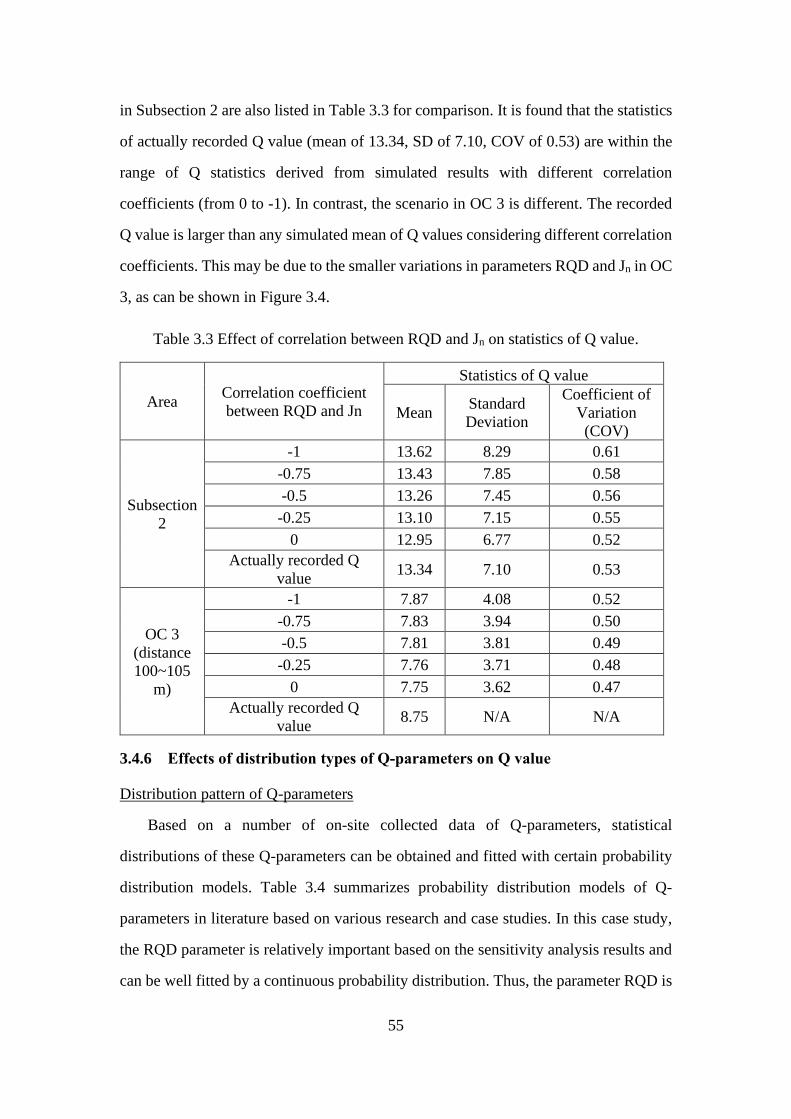
55
in Subsection 2 are also listed in Table 3.3 for comparison. It is found that the statistics
of actually recorded Q value (mean of 13.34, SD of 7.10, COV of 0.53) are within the
range of Q statistics derived from simulated results with different correlation
coefficients (from 0 to -1). In contrast, the scenario in OC 3 is different. The recorded
Q value is larger than any simulated mean of Q values considering different correlation
coefficients. This may be due to the smaller variations in parameters RQD and Jn in OC
3, as can be shown in Figure 3.4.
Table 3.3 Effect of correlation between RQD and Jn on statistics of Q value.
Area Correlation coefficient
between RQD and Jn
Statistics of Q value
Mean Standard
Deviation
Coefficient of
Variation
(COV)
Subsection
2
-1 13.62 8.29 0.61
-0.75 13.43 7.85 0.58
-0.5 13.26 7.45 0.56
-0.25 13.10 7.15 0.55
0 12.95 6.77 0.52
Actually recorded Q
value 13.34 7.10 0.53
OC 3
(distance
100~105
m)
-1 7.87 4.08 0.52
-0.75 7.83 3.94 0.50
-0.5 7.81 3.81 0.49
-0.25 7.76 3.71 0.48
0 7.75 3.62 0.47
Actually recorded Q
value 8.75 N/A N/A
3.4.6 Effects of distribution types of Q-parameters on Q value
Distribution pattern of Q-parameters
Based on a number of on-site collected data of Q-parameters, statistical
distributions of these Q-parameters can be obtained and fitted with certain probability
distribution models. Table 3.4 summarizes probability distribution models of Q-
parameters in literature based on various research and case studies. In this case study,
the RQD parameter is relatively important based on the sensitivity analysis results and
can be well fitted by a continuous probability distribution. Thus, the parameter RQD is
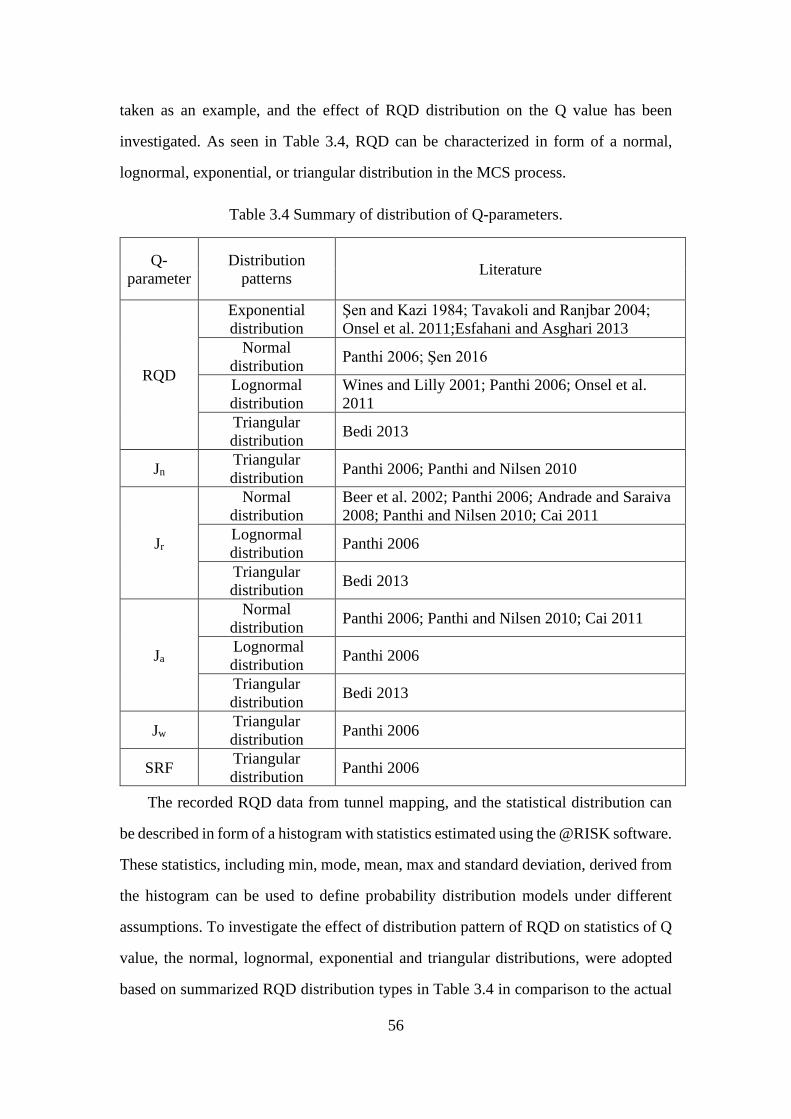
56
taken as an example, and the effect of RQD distribution on the Q value has been
investigated. As seen in Table 3.4, RQD can be characterized in form of a normal,
lognormal, exponential, or triangular distribution in the MCS process.
Table 3.4 Summary of distribution of Q-parameters.
Q-
parameter
Distribution
patterns Literature
RQD
Exponential
distribution
Şen and Kazi 1984; Tavakoli and Ranjbar 2004;
Onsel et al. 2011;Esfahani and Asghari 2013
Normal
distribution Panthi 2006; Şen 2016
Lognormal
distribution
Wines and Lilly 2001; Panthi 2006; Onsel et al.
2011
Triangular
distribution Bedi 2013
Jn Triangular
distribution Panthi 2006; Panthi and Nilsen 2010
Jr
Normal
distribution
Beer et al. 2002; Panthi 2006; Andrade and Saraiva
2008; Panthi and Nilsen 2010; Cai 2011
Lognormal
distribution Panthi 2006
Triangular
distribution Bedi 2013
Ja
Normal
distribution Panthi 2006; Panthi and Nilsen 2010; Cai 2011
Lognormal
distribution Panthi 2006
Triangular
distribution Bedi 2013
Jw Triangular
distribution Panthi 2006
SRF Triangular
distribution Panthi 2006
The recorded RQD data from tunnel mapping, and the statistical distribution can
be described in form of a histogram with statistics estimated using the @RISK software.
These statistics, including min, mode, mean, max and standard deviation, derived from
the histogram can be used to define probability distribution models under different
assumptions. To investigate the effect of distribution pattern of RQD on statistics of Q
value, the normal, lognormal, exponential and triangular distributions, were adopted
based on summarized RQD distribution types in Table 3.4 in comparison to the actual
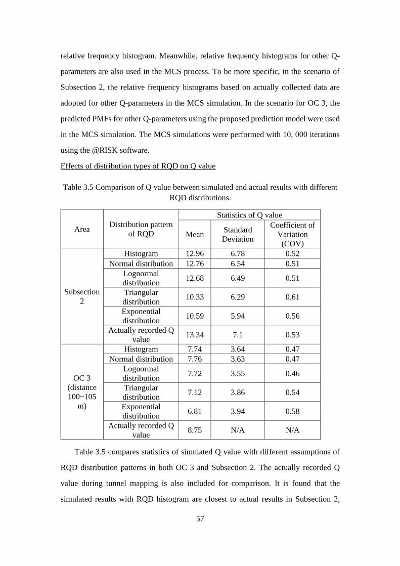
57
relative frequency histogram. Meanwhile, relative frequency histograms for other Q-
parameters are also used in the MCS process. To be more specific, in the scenario of
Subsection 2, the relative frequency histograms based on actually collected data are
adopted for other Q-parameters in the MCS simulation. In the scenario for OC 3, the
predicted PMFs for other Q-parameters using the proposed prediction model were used
in the MCS simulation. The MCS simulations were performed with 10, 000 iterations
using the @RISK software.
Effects of distribution types of RQD on Q value
Table 3.5 Comparison of Q value between simulated and actual results with different
RQD distributions.
Area Distribution pattern
of RQD
Statistics of Q value
Mean Standard
Deviation
Coefficient of
Variation
(COV)
Subsection
2
Histogram 12.96 6.78 0.52
Normal distribution 12.76 6.54 0.51
Lognormal
distribution 12.68 6.49 0.51
Triangular
distribution 10.33 6.29 0.61
Exponential
distribution 10.59 5.94 0.56
Actually recorded Q
value 13.34 7.1 0.53
OC 3
(distance
100~105
m)
Histogram 7.74 3.64 0.47
Normal distribution 7.76 3.63 0.47
Lognormal
distribution 7.72 3.55 0.46
Triangular
distribution 7.12 3.86 0.54
Exponential
distribution 6.81 3.94 0.58
Actually recorded Q
value 8.75 N/A N/A
Table 3.5 compares statistics of simulated Q value with different assumptions of
RQD distribution patterns in both OC 3 and Subsection 2. The actually recorded Q
value during tunnel mapping is also included for comparison. It is found that the
simulated results with RQD histogram are closest to actual results in Subsection 2,
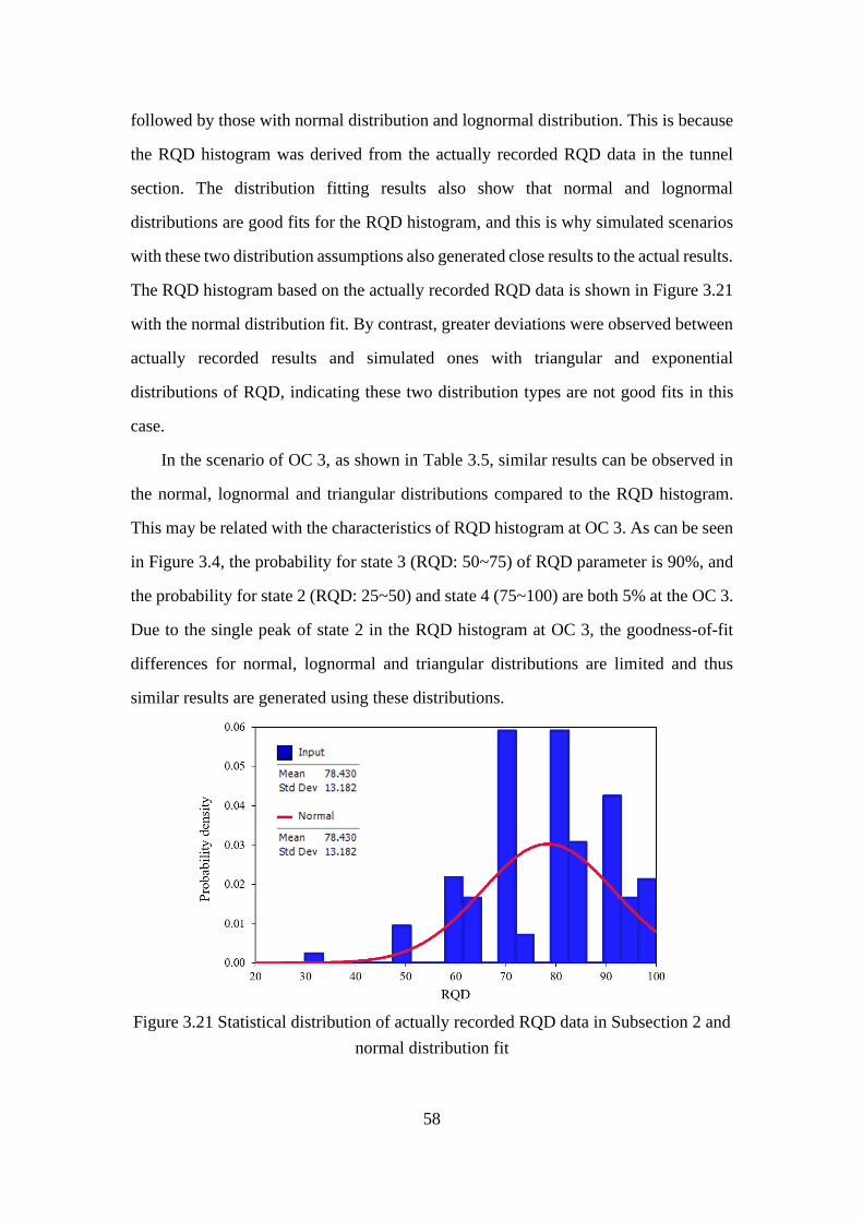
58
followed by those with normal distribution and lognormal distribution. This is because
the RQD histogram was derived from the actually recorded RQD data in the tunnel
section. The distribution fitting results also show that normal and lognormal
distributions are good fits for the RQD histogram, and this is why simulated scenarios
with these two distribution assumptions also generated close results to the actual results.
The RQD histogram based on the actually recorded RQD data is shown in Figure 3.21
with the normal distribution fit. By contrast, greater deviations were observed between
actually recorded results and simulated ones with triangular and exponential
distributions of RQD, indicating these two distribution types are not good fits in this
case.
In the scenario of OC 3, as shown in Table 3.5, similar results can be observed in
the normal, lognormal and triangular distributions compared to the RQD histogram.
This may be related with the characteristics of RQD histogram at OC 3. As can be seen
in Figure 3.4, the probability for state 3 (RQD: 50~75) of RQD parameter is 90%, and
the probability for state 2 (RQD: 25~50) and state 4 (75~100) are both 5% at the OC 3.
Due to the single peak of state 2 in the RQD histogram at OC 3, the goodness-of-fit
differences for normal, lognormal and triangular distributions are limited and thus
similar results are generated using these distributions.
Figure 3.21 Statistical distribution of actually recorded RQD data in Subsection 2 and
normal distribution fit
59
3.4.7 Perspective of the study
The proposed Q-based prediction model provides a framework for predicting rock
mass quality using the Markov Chain technique in the planning and preliminary design
stage of underground construction. The probability distributions of rock mass quality
can be predicted along the tunnel alignment before tunnel excavation based on site
investigation data, including the rock mass quality data in the regional area and
location-specific exploration boreholes. Note that the availability of Q data in the tunnel
area and boreholes are limited in this case study. In view of this, the Q data collected in
Subsection 1 of the excavated tunnel section was used as the input for the prediction
model, and Subsection 2 of the excavated tunnel section has been used as the test section,
considering the ground stationarity of the selected tunnel section. The proposed
probabilistic prediction model should also be applied to tunnel cases with Q data
available from the tunnel area and boreholes in the site investigation stage to test
prediction robustness. In addition, as reported by some researchers (Bieniawski, 1989;
Palmstrom and Stille, 2010), it is recommended to use more than one rock mass
classification (e.g. RMR, Q-system, GSI) in tunnel design for comparison. Thus, the
extension of the probabilistic Q-based prediction model to other rock mass
classification systems such as RMR and GSI should be incorporated into future work.
Further, the proposed prediction model should be updated based on new rock mass
quality data available during tunnel construction, and Bayesian updating technique or
equivalent can be used. It should also be noted that the selected tunnel section from the
water tunnel case study is in relatively stationary ground conditions. In a tunnel with
heterogeneous and complex geologic conditions, the tunnel section can be divided into
several relatively stationary subsections, and the Markov Chain-based prediction model
can be implemented in relatively stationary subsections. The proposed prediction model
should be applied to tunnel cases with more variable geologic conditions to test its
prediction performance for further study. Nevertheless, the proposed prediction model
enables the prediction of probabilistic distributions of rock mass quality along the
tunnel alignment before construction with a relative high prediction accuracy in this
60
case study, thus providing a supplement to the geology exploration and prospecting in
the planning and preliminary design stage of underground excavations.
3.5 Conclusions
The probabilistic distribution of rock mass quality Q index in the unexcavated
tunnel sections has been predicted before excavation by a Q-based prediction model
using the Markov chain technique. The proposed prediction model has been applied to
selected sections of a water tunnel for the purpose of validation. The predicted
probabilistic results of Q-parameter states, Q values and Q-based rock classes were
compared with those recorded during tunnel construction. The average prediction
accuracy for the predicted results was relatively high based on the accuracy plots in
comparison to the actually recorded Q data, indicating the effectiveness of the proposed
prediction model.
In addition to Monte Carlo-simulated results, an analytical calculation approach
for approximating the statistics of the Q value has also been developed given the
statistics of Q-parameters. The statistics of Q values estimated from the analytical
calculation approach were also compared to the MCS-derived and actually recorded Q
results, and the comparability among these results was confirmed.
Probabilistic sensitivity analysis was also carried out in the MCS process and
the relative importance of Q-parameters was ranked in tornado graphs based on four
different ranking criteria. All the ranking criteria show similar sensitivity results with
Jn and RQD being most influential, in consistent with the greater variations in the
predicted probabilistic profile of Jn and RQD compared to other Q-parameters.
Moreover, the negative correlation between RQD and Jn has been presented,
and the estimated mean and dispersion of the Q value would be underestimated if the
correlation was neglected. The effects of distribution for RQD on the Q value have also
been examined. The normal distribution was a good fit for the actually recorded RQD
data in this case study, and the generated Q value under this normal assumption of RQD
agreed well with the actually recorded Q results during tunnel construction.

61
The proposed Q-based prediction model is capable of quantitatively predicting
rock mass quality in the unexcavated tunnel section using a probabilistic approach and
can be used to complement geology exploration in the planning and preliminary design
stages of tunnel projects. It can also be helpful in probabilistically evaluating excavation
support strategies as well as the construction time and cost, thus contributing greatly to
decision support for the tunnel design and construction.
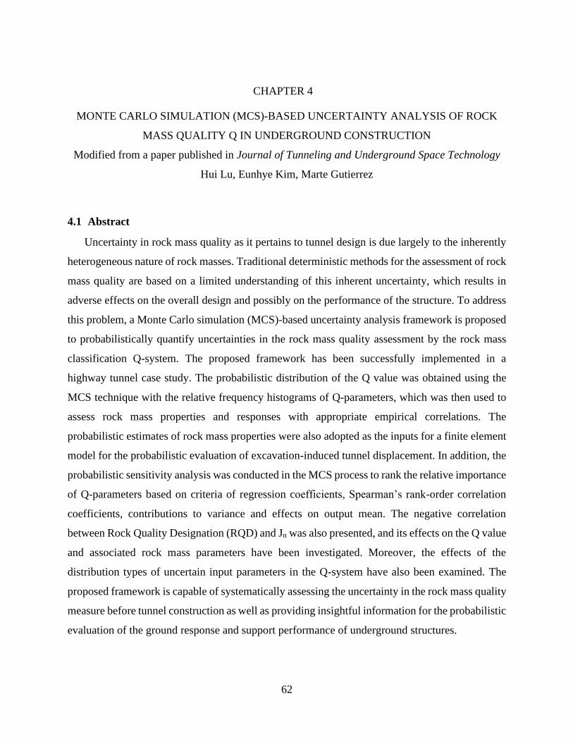
62
CHAPTER 4
MONTE CARLO SIMULATION (MCS)-BASED UNCERTAINTY ANALYSIS OF ROCK
MASS QUALITY Q IN UNDERGROUND CONSTRUCTION
Modified from a paper published in Journal of Tunneling and Underground Space Technology
Hui Lu, Eunhye Kim, Marte Gutierrez
4.1 Abstract
Uncertainty in rock mass quality as it pertains to tunnel design is due largely to the inherently
heterogeneous nature of rock masses. Traditional deterministic methods for the assessment of rock
mass quality are based on a limited understanding of this inherent uncertainty, which results in
adverse effects on the overall design and possibly on the performance of the structure. To address
this problem, a Monte Carlo simulation (MCS)-based uncertainty analysis framework is proposed
to probabilistically quantify uncertainties in the rock mass quality assessment by the rock mass
classification Q-system. The proposed framework has been successfully implemented in a
highway tunnel case study. The probabilistic distribution of the Q value was obtained using the
MCS technique with the relative frequency histograms of Q-parameters, which was then used to
assess rock mass properties and responses with appropriate empirical correlations. The
probabilistic estimates of rock mass properties were also adopted as the inputs for a finite element
model for the probabilistic evaluation of excavation-induced tunnel displacement. In addition, the
probabilistic sensitivity analysis was conducted in the MCS process to rank the relative importance
of Q-parameters based on criteria of regression coefficients, Spearman’s rank-order correlation
coefficients, contributions to variance and effects on output mean. The negative correlation
between Rock Quality Designation (RQD) and Jn was also presented, and its effects on the Q value
and associated rock mass parameters have been investigated. Moreover, the effects of the
distribution types of uncertain input parameters in the Q-system have also been examined. The
proposed framework is capable of systematically assessing the uncertainty in the rock mass quality
measure before tunnel construction as well as providing insightful information for the probabilistic
evaluation of the ground response and support performance of underground structures.
63
4.2 Introduction
Rock mass classification systems have been widely used to provide a quantitative assessment
of rock mass quality and guidelines for engineering design (Palmstrom and Stille, 2010). Empirical
rock mass classification systems, including the rock mass rating (RMR), rock mass quality Q-
system, and geological strength index (GSI), have inherent uncertainties (Palmstrom and Stille,
2007; Stille and Palmström, 2003). For example, in the Q-system, the joint characteristics, Jr, Ja
and especially Jn, in addition to the RQD, are prone to mischaracterization (Palmstrom and Broch,
2006). The traditional deterministic analysis methods, which are based on ground characterization
and rock mass classification, disregard the inherent uncertainties in the rock mass itself and thus
may cause conservative estimates to be used in the design and construction phases that inflate the
costs of underground construction (Guan et al., 2014; Ioannou, 1987).
The Q-log chart is commonly used to record the statistics of all the input parameters in the Q-
system for the field mapping of surface exposures, core logging or underground excavation
logging (Barton, 2002). The mean, mode and the range interval of each input parameter are
estimated based on the collected Q-log data, and these statistics for the overall Q value could be
calculated using an interval analysis. However, Panthi (2006) reported that the mean and range
values have poor statistical properties and are sensitive to extreme values. A Q-log example from
a case study showed that the typical Q value range was 0.008–100 with a mean value of 4.44
(Morelli, 2015). This cautious estimate of the range covers several rock classes, from exceptionally
“poor” to “extremely good”, and the mean value indicates that the rock mass is “fair” on average.
Bedi (2013) also reported that the lack of information on intervals could cause difficulty in
decision-making, as exemplified by the wide range of the calculated Q interval. In addition, if the
uncertainties and variabilities in the rock mass classifications are insufficiently characterized, they
may propagate through the design process and have an adverse impact on the ground response and
tunnel support performance (Baecher and Christian, 2003; Langford, 2013).
However, probabilistic analysis, which encompasses the complete probability distribution of
the rock mass parameters, is capable of adequately characterizing the uncertainties in rock mass
conditions. The probabilistic rock mass quality can capture the intrinsic and subjective variability
of the rock mass conditions and has a significant influence on the probabilistic design in
underground construction (Cai, 2011). Once uncertainties in the Q-system are quantified
probabilistically, probabilistic estimates of the rock mass properties can be made through a forward
64
uncertainty analysis based on the empirical relationships. The derived probabilistic rock mass
properties can be used as the inputs for a probabilistic analyses using numerical modeling, in which
the rock mass response and design performance can also be evaluated probabilistically. Sari (2009)
developed the probability distributions of the RMR and GSI based on probabilistic descriptions of
the discontinuities and intact rock properties using Monte Carlo simulation (MCS) and derived a
probabilistic estimate of the rock mass strength and deformability properties. Cai (2011) analyzed
GSI from probabilistic evaluations of the joint characteristics in field mapping and performed a
probabilistic analysis of tunnel and cavern stability which considered the variability of the rock
mass parameters and in situ stress.
Similarly, Tiwari et al. (2017) estimated the rock mass parameters from the GSI in tunnel case
studies and used them to assess the uncertainty in the yield zone and tunnel displacement. Idris et
al. (2015) quantified the deformation modulus of a rock mass at the Laisvall mine based on the
probabilistic distribution of GSI and adopted it to evaluate the pillar stability using numerical
simulations. Bedi (2013) developed the probability density distribution (PDF) of the Q value in
the Gjovik cavern using the MCS technique based on triangular PDFs of Q-parameters.
However, no attempts in the past research have been made to consider the relative importance
of the input parameters in the probabilistic Q-system. Additionally, the majority of studies fail to
take into account the interdependencies between uncertain Q-parameters and the effects of the
distribution types of the Q-parameters. In this chapter, an MCS-based uncertainty analysis
framework for the Q-system has been proposed. By conducting the MCS, the probabilistic
sensitivity analysis has been used to investigate the impact of the input parameters on the Q-system
and associated rock mass parameters. The effects of the correlations between input parameters and
the effects of the input parameter distribution types on the Q value and associated rock mass
properties and responses have also been examined. The proposed MCS-based uncertainty analysis
framework for the Q-system is described in detail in Section 4.3, in which the MCS-based
stochastic model of the rock mass quality Q and the uncertainty analysis of the probabilistic Q-
system are introduced. The framework has been implemented in a case study of the Shimizu
highway tunnel in Japan for illustrative purposes. The results and discussion on the case study are
in Section 4.4, followed by the major conclusions in Section 4.5.
65
4.3 Methodology
4.3.1 Stochastic modeling of the rock mass quality
Probabilistic Q value from Monte Carlo simulation
The MCS is a stochastic simulation method where the distribution of possible outcomes is
produced from different randomly sampled sets of values from the probability distributions of the
input parameters. The probability distribution is specified for each input parameter, and the
randomly selected input values are used to simulate a wide range of possible output values
(Palisade Corporation, 2016). The disadvantages of MCS are that it requires substantial
computational resources, along with explicit probability distribution functions for the input
variables (Cai, 2011). For a more comprehensive description of MCS, the reader can refer to the
literature (Gentle, 2013; Law et al., 1991; Vose, 2008).
The Excel add-in program @RISK is an advanced statistical risk analysis system that
implements MCS in a standard spreadsheet package, in which the uncertainty in the input
parameters can be explicitly characterized to produce outputs that describe all the possible
outcomes (Palisade Corporation, 2016). It allows the definition of different types of continuous
and discrete probability distributions for the input parameters in the spreadsheet, and it is capable
of making a best-fit for the available data as well as generating statistics for the data and the fit
curve. The @RISK program enables stochastic simulation using both Monte Carlo and Latin
hypercube sampling techniques for any number of iterations per simulation and any number of
simulations in a single analysis (Palisade Corporation, 2016). For the Monte Carlo sampling,
samples are more likely to be drawn from the areas of the distribution that have a higher probability
of occurrence due to its entirely random feature. Clustering becomes an issue when a distribution
includes low probability outcomes, which could have a major impact on the results, especially
when a small number of iterations are carried out.
In contrast, the Latin Hypercube sampling requires fewer iterations due to the use of stratified
sampling from the input probability distributions. Stratification divides the cumulative density
function (CDF) of the input parameter into equal intervals, and a sample is then randomly selected
from each interval or stratification of the input probability distribution. Sampling thus draws
representative samples from each interval, which then recreates and more accurately reflects the
input probability distribution. Compared with traditional Monte Carlo sampling, Latin hypercube
sampling provides increased sampling efficiency and faster runtimes due to fewer iterations. The
66
Latin hypercube sampling also aids the analysis in situations where low probability outcomes are
represented in the input probability distributions (Palisade Corporation, 2016).
In the Q-system, all the input parameters can be regarded as random variables. The
variability of the input parameters can be described by their relative frequency histograms, which
can be accessed from the Q-histogram logging data by drilled core logging, exposed outcrop
mapping, and tunnel mapping. When the statistical distributions are developed for the six input
parameters, the distribution of the Q value can be calculated according to Eq. (2.1) using MCS
with Latin hypercube sampling in the @RISK program. The Q-input parameter values are
randomly sampled from their distributions, and the probability distribution of the Q value is
generated from the simulation runs. A statistical analysis can be performed on the probability
distribution of the Q value that is produced, and the statistics for rock mass quality can be derived.
Probabilistic evaluation of the rock mass properties and responses
Once the probability distributions of the Q value and other input parameters have been
determined, the rock mass properties and responses can be similarly characterized probabilistically
according to empirical equations using the MCS with the @RISK program.
parameters (e.g., the tunnel wall displacement or the radius of the plastic zone), either an MCS or
the point estimate method (PEM) (Rosenblueth, 1981) can be used for the numerical analysis. The
RS2 FEM program is capable of performing probabilistic analysis using MCS with both Monte
Carlo and Latin Hypercube sampling as well as PEM techniques. The MCS and PEM techniques
can be used to probabilistically characterize the uncertainties in the input parameters of the
numerical model.
Table 4.1 and Table 4.2 list the empirical correlations between the Q value and the rock mass
properties and responses, respectively. The parameters that must be calculated for the rock mass
responses include the displacement and plastic zone radius of the underground opening; based on
Hoek and Marinos (2000b), the Duncan Fama (1993), and the Barton (2002) approach, are
introduced. Note that the Q-based empirical correlations for evaluating the rock mass responses
only serve as a preliminary estimation. These empirical correlations were either derived using
several simplified theoretical assumptions or obtained from the databases of different case histories.
For a more reliable and accurate assessment of the rock mass responses of underground
excavations, a numerical analysis should be conducted.
Probabilistic analysis of the rock mass response with numerical modeling
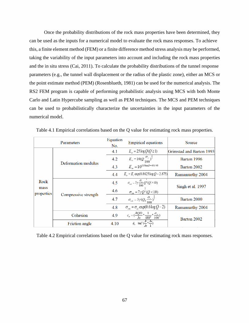
67
Once the probability distributions of the rock mass properties have been determined, they
can be used as the inputs for a numerical model to evaluate the rock mass responses. To achieve
this, a finite element method (FEM) or a finite difference method stress analysis may be performed,
taking the variability of the input parameters into account and including the rock mass properties
and the in situ stress (Cai, 2011). To calculate the probability distributions of the tunnel response
parameters (e.g., the tunnel wall displacement or the radius of the plastic zone), either an MCS or
the point estimate method (PEM) (Rosenblueth, 1981) can be used for the numerical analysis. The
RS2 FEM program is capable of performing probabilistic analysis using MCS with both Monte
Carlo and Latin Hypercube sampling as well as PEM techniques. The MCS and PEM techniques
can be used to probabilistically characterize the uncertainties in the input parameters of the
numerical model.
Table 4.1 Empirical correlations based on the Q value for estimating rock mass properties.
Table 4.2 Empirical correlations based on the Q value for estimating rock mass responses.
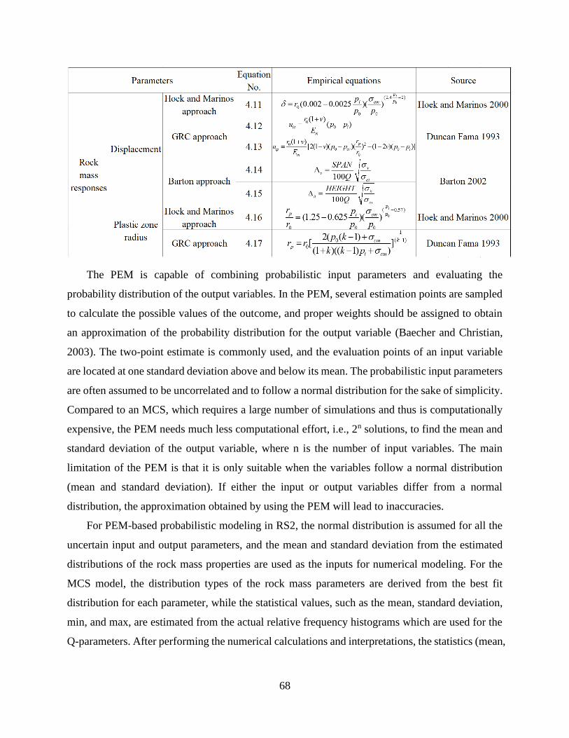
68
The PEM is capable of combining probabilistic input parameters and evaluating the
probability distribution of the output variables. In the PEM, several estimation points are sampled
to calculate the possible values of the outcome, and proper weights should be assigned to obtain
an approximation of the probability distribution for the output variable (Baecher and Christian,
2003). The two-point estimate is commonly used, and the evaluation points of an input variable
are located at one standard deviation above and below its mean. The probabilistic input parameters
are often assumed to be uncorrelated and to follow a normal distribution for the sake of simplicity.
Compared to an MCS, which requires a large number of simulations and thus is computationally
expensive, the PEM needs much less computational effort, i.e., 2n solutions, to find the mean and
standard deviation of the output variable, where n is the number of input variables. The main
limitation of the PEM is that it is only suitable when the variables follow a normal distribution
(mean and standard deviation). If either the input or output variables differ from a normal
distribution, the approximation obtained by using the PEM will lead to inaccuracies.
For PEM-based probabilistic modeling in RS2, the normal distribution is assumed for all the
uncertain input and output parameters, and the mean and standard deviation from the estimated
distributions of the rock mass properties are used as the inputs for numerical modeling. For the
MCS model, the distribution types of the rock mass parameters are derived from the best fit
distribution for each parameter, while the statistical values, such as the mean, standard deviation,
min, and max, are estimated from the actual relative frequency histograms which are used for the
Q-parameters. After performing the numerical calculations and interpretations, the statistics (mean,

69
standard deviation) of the rock mass response parameters can be obtained at arbitrary points in the
model based on a certain number of iterations.
4.3.2 Uncertainty analysis in the Q-system
Probabilistic sensitivity analysis in the Q-system
The sensitivity analysis of the Q value to its input parameters can be conducted in the @RISK
program. The sensitivity analysis results are shown using tornado graphs that display the rank of
the input distributions relative to the impact on the output distribution. Inputs with the largest
impact on the output distribution have the longest (and topmost) bars in the graph (Palisade
Corporation, 2016). Four tornado graphs in @RISK are commonly used for ranking the relative
importance of input parameters: the regression coefficients, the Spearman correlation coefficients,
the contribution to output variance, and the effect on output mean. For the tornado graphs showing
regression coefficients or Spearman correlation coefficients, the length of the bar shown for each
input distribution is based on the coefficient value calculated between the output and the input
parameter. It should be noted that the regression coefficient describes the size of the effect each
input has on the output. In contrast, the correlation coefficient indicates whether increasing the
input generally increases or decreases the output and how consistent that trend is, but it tells
nothing about the strength of the influence. In the @RISK program, the regression coefficient for
an input variable shown on a tornado graph is the scaled value normalized by its standard deviation
and the standard deviation of the output, which also reflects the impact of the input parameters on
the output. For tornado graphs showing the contribution to variance, the length of the bar is the
amount of change in the output attributable to each input. These values are calculated during the
regression analysis. Unlike a regression coefficient, this measurement is unaffected by the
magnitude of the input. In the tornado graph, to visualize the effect on the output mean, the double-
sided tornado has one bar for each selected input. The output means are calculated for the output
values in each iteration as the input varies over its range.
In the tornado graphs, the numbers shown at the two ends of a bar graph describe the calculated
values for the different ranking techniques used during the simulation process. Note that the
numbers at the two ends of the double-sided tornado, showing the effect on the output mean, are
the means of the output variable from the iterations with the lowest and highest 10% of input
values, respectively. The rank of the input parameters is based on the range between the highest
and the lowest mean value caused by that input parameter, i.e., the length of the bar. The regression
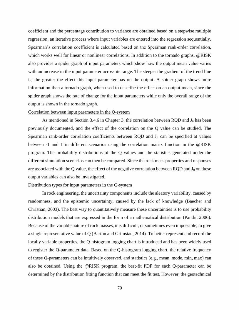
70
coefficient and the percentage contribution to variance are obtained based on a stepwise multiple
regression, an iterative process where input variables are entered into the regression sequentially.
Spearman’s correlation coefficient is calculated based on the Spearman rank-order correlation,
which works well for linear or nonlinear correlations. In addition to the tornado graphs, @RISK
also provides a spider graph of input parameters which show how the output mean value varies
with an increase in the input parameter across its range. The steeper the gradient of the trend line
is, the greater the effect this input parameter has on the output. A spider graph shows more
information than a tornado graph, when used to describe the effect on an output mean, since the
spider graph shows the rate of change for the input parameters while only the overall range of the
output is shown in the tornado graph.
Correlation between input parameters in the Q-system
As mentioned in Section 3.4.6 in Chapter 3, the correlation between RQD and Jn has been
previously documented, and the effect of the correlation on the Q value can be studied. The
Spearman rank-order correlation coefficients between RQD and Jn can be specified at values
between -1 and 1 in different scenarios using the correlation matrix function in the @RISK
program. The probability distributions of the Q values and the statistics generated under the
different simulation scenarios can then be compared. Since the rock mass properties and responses
are associated with the Q value, the effect of the negative correlation between RQD and Jn on these
output variables can also be investigated.
Distribution types for input parameters in the Q-system
In rock engineering, the uncertainty components include the aleatory variability, caused by
randomness, and the epistemic uncertainty, caused by the lack of knowledge (Baecher and
Christian, 2003). The best way to quantitatively measure these uncertainties is to use probability
distribution models that are expressed in the form of a mathematical distribution (Panthi, 2006).
Because of the variable nature of rock masses, it is difficult, or sometimes even impossible, to give
a single representative value of Q (Barton and Grimstad, 2014). To better represent and record the
locally variable properties, the Q-histogram logging chart is introduced and has been widely used
to register the Q-parameter data. Based on the Q-histogram logging chart, the relative frequency
of these Q-parameters can be intuitively observed, and statistics (e.g., mean, mode, min, max) can
also be obtained. Using the @RISK program, the best-fit PDF for each Q-parameter can be
determined by the distribution fitting function that can meet the fit test. However, the geotechnical
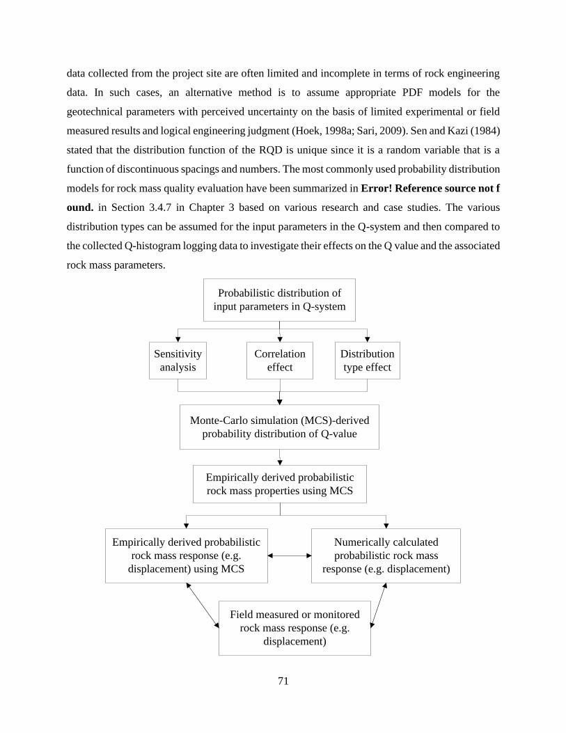
71
data collected from the project site are often limited and incomplete in terms of rock engineering
data. In such cases, an alternative method is to assume appropriate PDF models for the
geotechnical parameters with perceived uncertainty on the basis of limited experimental or field
measured results and logical engineering judgment (Hoek, 1998a; Sari, 2009). Sen and Kazi (1984)
stated that the distribution function of the RQD is unique since it is a random variable that is a
function of discontinuous spacings and numbers. The most commonly used probability distribution
models for rock mass quality evaluation have been summarized in Error! Reference source not f
ound. in Section 3.4.7 in Chapter 3 based on various research and case studies. The various
distribution types can be assumed for the input parameters in the Q-system and then compared to
the collected Q-histogram logging data to investigate their effects on the Q value and the associated
rock mass parameters.
Probabilistic distribution of
input parameters in Q-system
Monte-Carlo simulation (MCS)-derived
probability distribution of Q-value
Empirically derived probabilistic
rock mass properties using MCS
Empirically derived probabilistic
rock mass response (e.g.
displacement) using MCS
Numerically calculated
probabilistic rock mass
response (e.g. displacement)
Field measured or monitored
rock mass response (e.g.
displacement)
Sensitivity
analysis
Correlation
effect
Distribution
type effect
72
Figure 4.1 Block diagram of the proposed framework.
The proposed framework is illustrated in Figure 4.1. The uncertainty in the rock mass is
characterized by the probability distribution of input parameters in the Q-system. Using the MCS
technique, the probability distribution of the Q value, rock mass properties and responses (e.g.
displacement, plastic radius) can be obtained based on the Q-derived empirical relationships. In
this process, the uncertainty is propagated from the Q-parameters to the Q value and to the Q-
based rock mass parameters. To quantitatively characterize the process, the sensitivity analysis,
the effects of the correlation, and the effects of distribution types among the input parameters in
the Q-system can be performed. On one hand, the empirically derived probabilistic rock mass
properties can be used to evaluate the rock mass responses empirically using the MCS technique;
on the other hand, these probabilistic rock mass properties can also serve as the input in numerical
modeling to estimate the probabilistic distribution of rock mass responses. The empirically and
numerically derived probabilistic distribution of rock mass responses can be compared with each
other and should be validated in comparison to the field measured or monitored rock mass response
data.
4.3.3 Application to a case study of the Shimizu tunnel
The Shimizu tunnel No. 3, located in the city of Shimizu in Japan, is an important section
of Japan’s Tomei-Meishin Expressway project. It is a research tunnel with a length of 1.12 km
(height 12 m, width 18 m). The depth varies from 30 m to 190 m with an average of approximately
83 m. The average in-situ stresses are 2 MPa and 1.73 MPa in the vertical and horizontal directions,
respectively, giving a stress ratio of 0.83 (Vardakos, 2003). Figure 4.2 shows the longitudinal
geologic section along the western and central sector tunnel. Field investigations showed that the
ground was composed of soft sedimentary rock formations, including weathered soft sandstone
(Wss) and interbedded mudstone-sandstone (Walt 1 and Walt 2). The tunnel was excavated mainly
through the Wss sandstone formation with a density of 2.5 g/cm3. Three major joint sets were
recognized in the weathered soft sandstone. The geotechnical data are collected by the Norwegian
Geotechnical Institute by inspecting drilled cores, field mapping, geophysical investigations and
laboratory tests on intact rock samples, and a detailed Q logging was made (Barton et al., 1995).
Core logging was carried out for a total of four selected drill cores in the western and central sector
from the Shimizu tunnel site. Two horizontal borings were drilled in the western portals with about
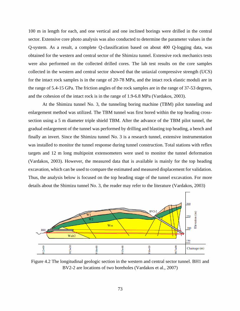
73
100 m in length for each, and one vertical and one inclined borings were drilled in the central
sector. Extensive core photo analysis was also conducted to determine the parameter values in the
Q-system. As a result, a complete Q-classification based on about 400 Q-logging data, was
obtained for the western and central sector of the Shimizu tunnel. Extensive rock mechanics tests
were also performed on the collected drilled cores. The lab test results on the core samples
collected in the western and central sector showed that the uniaxial compressive strength (UCS)
for the intact rock samples is in the range of 20-78 MPa, and the intact rock elastic moduli are in
the range of 5.4-15 GPa. The friction angles of the rock samples are in the range of 37-53 degrees,
and the cohesion of the intact rock is in the range of 1.9-6.8 MPa (Vardakos, 2003).
At the Shimizu tunnel No. 3, the tunneling boring machine (TBM) pilot tunneling and
enlargement method was utilized. The TBM tunnel was first bored within the top heading cross-
section using a 5 m diameter triple shield TBM. After the advance of the TBM pilot tunnel, the
gradual enlargement of the tunnel was performed by drilling and blasting top heading, a bench and
finally an invert. Since the Shimizu tunnel No. 3 is a research tunnel, extensive instrumentation
was installed to monitor the tunnel response during tunnel construction. Total stations with reflex
targets and 12 m long multipoint extensometers were used to monitor the tunnel deformation
(Vardakos, 2003). However, the measured data that is available is mainly for the top heading
excavation, which can be used to compare the estimated and measured displacement for validation.
Thus, the analysis below is focused on the top heading stage of the tunnel excavation. For more
details about the Shimizu tunnel No. 3, the reader may refer to the literature (Vardakos, 2003)
Figure 4.2 The longitudinal geologic section in the western and central sector tunnel. BH1 and
BV2-2 are locations of two boreholes (Vardakos et al., 2007)
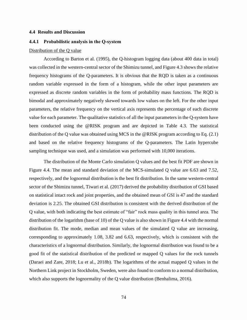
74
4.4 Results and Discussion
4.4.1 Probabilistic analysis in the Q-system
Distribution of the Q value
According to Barton et al. (1995), the Q-histogram logging data (about 400 data in total)
was collected in the western-central sector of the Shimizu tunnel, and Figure 4.3 shows the relative
frequency histograms of the Q-parameters. It is obvious that the RQD is taken as a continuous
random variable expressed in the form of a histogram, while the other input parameters are
expressed as discrete random variables in the form of probability mass functions. The RQD is
bimodal and approximately negatively skewed towards low values on the left. For the other input
parameters, the relative frequency on the vertical axis represents the percentage of each discrete
value for each parameter. The qualitative statistics of all the input parameters in the Q-system have
been conducted using the @RISK program and are depicted in Table 4.3. The statistical
distribution of the Q value was obtained using MCS in the @RISK program according to Eq. (2.1)
and based on the relative frequency histograms of the Q-parameters. The Latin hypercube
sampling technique was used, and a simulation was performed with 10,000 iterations.
The distribution of the Monte Carlo simulation Q values and the best fit PDF are shown in
Figure 4.4. The mean and standard deviation of the MCS-simulated Q value are 6.63 and 7.52,
respectively, and the lognormal distribution is the best fit distribution. In the same western-central
sector of the Shimizu tunnel, Tiwari et al. (2017) derived the probability distribution of GSI based
on statistical intact rock and joint properties, and the obtained mean of GSI is 47 and the standard
deviation is 2.25. The obtained GSI distribution is consistent with the derived distribution of the
Q value, with both indicating the best estimate of “fair” rock mass quality in this tunnel area. The
distribution of the logarithm (base of 10) of the Q value is also shown in Figure 4.4 with the normal
distribution fit. The mode, median and mean values of the simulated Q value are increasing,
corresponding to approximately 1.08, 3.82 and 6.63, respectively, which is consistent with the
characteristics of a lognormal distribution. Similarly, the lognormal distribution was found to be a
good fit of the statistical distribution of the predicted or mapped Q values for the rock tunnels
(Daraei and Zare, 2018; Lu et al., 2018b). The logarithms of the actual mapped Q values in the
Northern Link project in Stockholm, Sweden, were also found to conform to a normal distribution,
which also supports the lognormality of the Q value distribution (Benhalima, 2016).
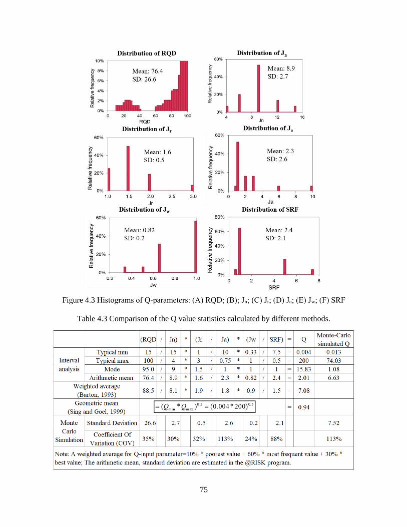
75
Figure 4.3 Histograms of Q-parameters: (A) RQD; (B); Jn; (C) Jr; (D) Ja; (E) Jw; (F) SRF
Table 4.3 Comparison of the Q value statistics calculated by different methods.

76
Traditionally, an interval analysis based on the statistics obtained from the Q-histogram
logging in the site investigation stage is used to estimate the Q value. Table 4.3 compares the
statistics of the Q value calculated from different methods. The interval analysis results show that
the Q value is in the range of 0.004-200, from “exceptionally poor” to “exceptionally good”, based
on the rock mass classification. The arithmetic mean and mode (most frequent value) of the Q
value is also calculated directly by substituting the mean and mode of all the Q-parameters into
Eq. (2.1), giving mean and mode values of 2.01 and 15.83, respectively. For the derivation of the
typical min and max of the output Q value, the extreme values are selected for input parameters,
and it is based on the assumption that the numerators for all the input parameters are achieved at
the maximum (or minimum) values while at the same time the denominators are achieved at the
minimum (or maximum) values. In other words, all the numerators (or denominators) are assumed
perfectly positively correlated while perfectly negative correlations are assumed between
numerators and denominators. Similarly, for the derivation of mode and mean of the Q value, the
respective mode and mean values for each input Q-parameter are used. This is assumed that the
mode and mean values for all the Q-parameters take place simultaneously. These idealized
assumptions are not logical and rarely met in practice. Clearly, these derivation processes using
the interval analysis do not realistically reflect the relationship among the input parameters in the
Q-system and the derived range is relatively large.
By contrast, the Monte Carlo simulated Q value has a much narrower range (0.013-74.03)
with a mean and mode of 6.63 and 1.08, respectively, as shown in Figure 4.4. The standard
deviation and the arithmetic mean were obtained for each Q-parameter and the overall Q value in
the @RISK program. The coefficient of variation (COV), a dimensionless measure of uncertainty
and defined as the quotient between the standard deviation and the mean, was also obtained for
the Q-parameters and the Q value in Table 4.3. To ensure the selection of representative values for
the Q-parameters, Barton (1993) proposed a method to calculate the weighted average value for
each Q-parameter. First, the weighted average value, calculated by adding the 10% poorest, 60%
most typical and 30% best values, is obtained for each Q-parameter. Then, the weighted average
Q value is obtained by substituting the weighted average values of all the Q-parameters into Eq.
(2.1). The calculated weighted average Q value is 7.08, which is close to the mean (6.63) of the
Monte Carlo simulation Q value. Singh and Goel (1999) also suggested that a geometric mean
obtained from the minimum and maximum values can be considered as a representative Q value,
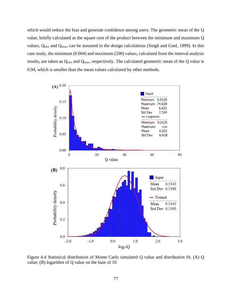
77
which would reduce the bias and generate confidence among users. The geometric mean of the Q
value, briefly calculated as the square root of the product between the minimum and maximum Q
values, Qmin and Qmax, can be assumed in the design calculations (Singh and Goel, 1999). In this
case study, the minimum (0.004) and maximum (200) values, calculated from the interval analysis
results, are taken as Qmin and Qmax, respectively. The calculated geometric mean of the Q value is
0.94, which is smaller than the mean values calculated by other methods.
Figure 4.4 Statistical distribution of Monte Carlo simulated Q value and distribution fit. (A) Q
value; (B) logarithm of Q value on the base of 10
78
From the results, the Monte Carlo simulation is superior to the interval analysis in
estimating the statistics of the Q value. The MCS technique can more realistically account for the
correlations, e.g. RQD and Jn, among input parameters and provides the full probability
distribution and a much narrower range for the Q value compared with the interval analysis method.
The probability that the Q value would be less than a certain value or in a certain interval could be
determined from the PDF or CDF of the Monte Carlo-simulated Q value. By contrast, the interval
analysis only produces an interval that provides little information with which to make an
engineering design decision, and the uncertainty is too large to make a subjective judgment (Bedi,
2013). In addition, the statistics of the Q value calculated using the MCS are more reliable than
those from the interval analysis. The statistics (min, max, arithmetic mean, standard deviation,
mode, and median) of the Monte Carlo simulation Q value were obtained based on a larger number
(10,000 in this case) of generated samples during the MCS process. In contrast, in the interval
analysis the mean and mode of the Q value are directly calculated from the mean and mode of all
the input parameters. In the calculation of the mean Q value during the MCS process, the effect of
the standard deviations of the Q-parameters has been taken into account. By contrast, this effect is
neglected in the interval analysis and may lead to some inaccuracies. Table 4.3 also shows that the
calculated mode (15.83) is much larger than the arithmetic mean (2.01) in the interval analysis,
while the mode (1.08) is smaller than the mean (6.63) in the Monte Carlo simulation results.
According to the lognormality of the Q value distribution, the mode should be smaller than the
arithmetic mean. In this sense, the Monte Carlo simulation results reflect the characteristics of a
lognormal distribution for the Q value. Furthermore, the standard deviation, a measure of spread,
can be obtained for each input parameter and the generated Q value in the MCS process.
Consequently, the COV can be calculated for each input parameter and enables the quantitative
characterization of uncertainty in the input parameters and the effects on the overall Q value.
In addition to the interval analysis, both the geometric mean and the weighted average
calculations are deterministic approaches to obtaining a representative value of the Q index. By
definition, the geometric mean is calculated as the nth root of the product of n (nonnegative) random
variables (Fenton and Griffiths, 2008). However, in the geometric mean calculation method used
by Barton (1993), only the extreme values, i.e., the minimum and maximum, are included in the
calculation for the geometric mean of the Q value. The result is highly sensitive to the extreme
values, and the role that other Q values in the Q value range play in the geometric mean value has
79
been overlooked. A geometric mean Q value of 0.94 was generated, which greatly underestimated
the actual rock mass quality. In comparison to the geometric mean, the weighted average method
(Barton, 1993) accounts for the effect of the mode in addition to the extreme values in the input
parameters. As a result, the weighted average (7.08) is closer to the mean (6.63) of the Monte Carlo
simulation Q value. However, both the geometric mean and weighted average methods do not
provide the full probability distribution of the Q value and do not reflect the uncertainties involved.
Thus, it is also inferior to the MCS method in probabilistically estimating the Q value.
Probability distributions of the rock mass properties and responses
Table 4.4 lists the Q-based empirical relationships for estimating the rock mass properties
and responses for the Shimizu tunnel case study. There are two approaches for estimating the rock
mass properties from the Q value, i.e., the independent and normalized estimation approaches
(Vásárhelyi and Kovács, 2017; Zhang, 2017). In the independent approach the rock mass
properties can be calculated independently of the intact rock properties, and thus Eqs. (2-4) and (7)
belong to this approach. By contrast, the normalized estimation approach indicates the dependence
of the rock mass properties on the intact rock properties, and Eqs. (5) and (9) are examples of this
approach. The intact rock properties are also included in Table 4.4 for comparison. The UCS and
the elastic modulus of the intact rock samples are assumed to follow a normal and a lognormal
distribution, respectively, which is based on published data from the literature (Hoek, 1998a; Li
and Low, 2010; Sari, 2009; Tiwari et al., 2017). The means and standard deviations of the
distributions for the intact rock parameters are estimated using the three sigma rule. The
independent estimating approach does not work well in this case study since the estimated elastic
modulus values of the rock mass are even larger than those of the intact rock as seen by comparing
the mean (10.2) of the intact rock with the mean values calculated by Eqs. (2-4). This is not
reasonable and should be discarded. Additionally, the rock mass elastic modulus calculated from
Eq. (4.1) shows the minimum value as negative, which is not physically possible. This is because
there is approximately an 18% probability that the Q value is smaller than 1, as can be estimated
from Figure 4.4, and the logarithms of values less than 1 yield negative results. Recall that Eq.
(4.1) in
parameters (e.g., the tunnel wall displacement or the radius of the plastic zone), either an MCS or
the point estimate method (PEM) (Rosenblueth, 1981) can be used for the numerical analysis. The
RS2 FEM program is capable of performing probabilistic analysis using MCS with both Monte
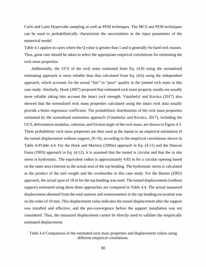
80
Carlo and Latin Hypercube sampling as well as PEM techniques. The MCS and PEM techniques
can be used to probabilistically characterize the uncertainties in the input parameters of the
numerical model.
Table 4.1 applies to cases where the Q value is greater than 1 and is generally for hard rock masses.
Thus, great care should be taken to select the appropriate empirical correlations for estimating the
rock mass properties.
Additionally, the UCS of the rock mass estimated from Eq. (4.8) using the normalized
estimating approach is more reliable than that calculated from Eq. (4.6) using the independent
approach, which accounts for the actual “fair” to “poor” quality in the jointed rock mass in this
case study. Similarly, Hoek (2007) proposed that estimated rock mass property results are usually
more reliable taking into account the intact rock strength. Vásárhelyi and Kovács (2017) also
showed that the normalized rock mass properties calculated using the intact rock data usually
provide a better regression coefficient. The probabilistic distributions of the rock mass properties
estimated by the normalized estimation approach (Vásárhelyi and Kovács, 2017), including the
UCS, deformation modulus, cohesion, and friction angle of the rock mass, are shown in Figure 4.5.
These probabilistic rock mass properties are then used as the inputs to an empirical estimation of
the tunnel displacement without support, (Pi=0), according to the empirical correlations shown in
Table 4.4Table 4.4. For the Hoek and Marinos (2000a) approach in Eq. (4.11) and the Duncan
Fama (1993) approach in Eq. (4.12), it is assumed that the tunnel is circular and that the in situ
stress is hydrostatic. The equivalent radius is approximately 4.83 m for a circular opening based
on the same area criterion as the actual area of the top heading. The hydrostatic stress is calculated
as the product of the unit weight and the overburden in this case study. For the Barton (2002)
approach, the actual span of 18 m for the top heading was used. The tunnel displacements (without
support) estimated using these three approaches are compared in Table 4.4. The actual measured
displacement obtained from the total stations and extensometers in the top heading excavation was
on the order of 10 mm. This displacement value indicates the tunnel displacement after the support
was installed and effective, and the pre-convergence before the support installation was not
considered. Thus, the measured displacement cannot be directly used to validate the empirically
estimated displacement.
Table 4.4 Comparison of the estimated rock mass properties and displacement values using
different empirical correlations.
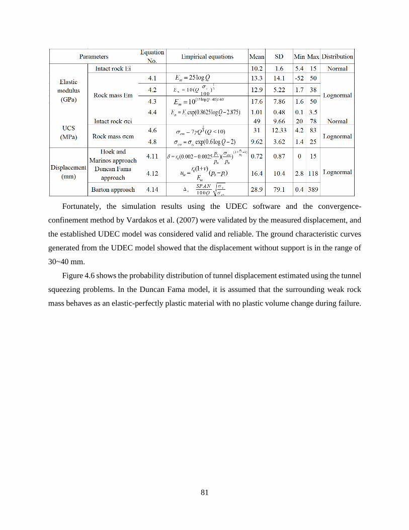
81
Fortunately, the simulation results using the UDEC software and the convergence-
confinement method by Vardakos et al. (2007) were validated by the measured displacement, and
the established UDEC model was considered valid and reliable. The ground characteristic curves
generated from the UDEC model showed that the displacement without support is in the range of
30~40 mm.
Figure 4.6 shows the probability distribution of tunnel displacement estimated using the tunnel
squeezing problems. In the Duncan Fama model, it is assumed that the surrounding weak rock
mass behaves as an elastic-perfectly plastic material with no plastic volume change during failure.
82
Figure 4.5 Statistical distributions of estimated rock mass properties. (A) UCS; (B) deformation
modulus; (C) cohesion; (D) friction angle
According to the derived Q value and rock mass properties, this approach does not fit the case of
the Shimizu tunnel. Thus, the Hoek and Marinos approach and the Duncan Fama approach, which
work best for weak and very weak rock masses with assumptions of a circular tunnel and
hydrostatic stress, are not suitable for estimating tunnel displacement in the current case study. In
contrast, the Barton approach, empirically derived from hundreds of case records, uses the actual
tunnel span and does not restrict the stress conditions, thus providing a more reliable estimate of
tunnel displacement. Therefore, for this case study, the Barton approach performs better for
empirically deriving the preliminary estimate of the tunnel displacement, which can be compared
with the displacement generated from the detailed analysis using the FEM numerical modeling
program.
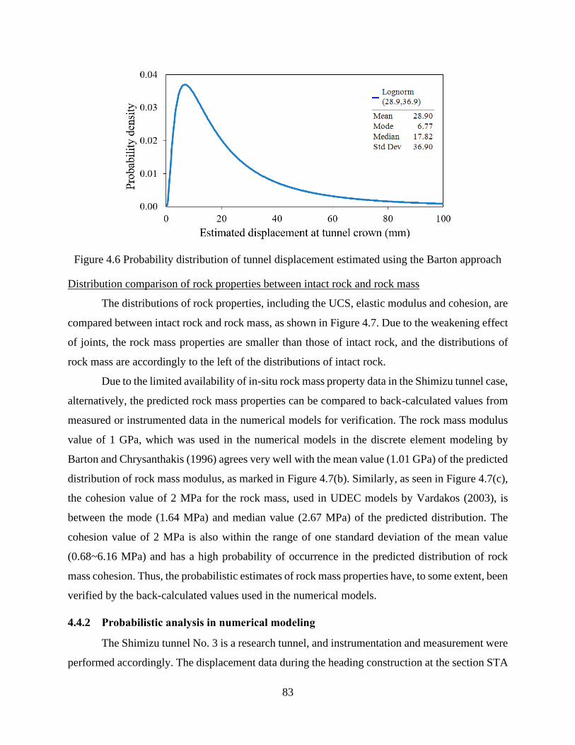
83
Figure 4.6 Probability distribution of tunnel displacement estimated using the Barton approach
Distribution comparison of rock properties between intact rock and rock mass
The distributions of rock properties, including the UCS, elastic modulus and cohesion, are
compared between intact rock and rock mass, as shown in Figure 4.7. Due to the weakening effect
of joints, the rock mass properties are smaller than those of intact rock, and the distributions of
rock mass are accordingly to the left of the distributions of intact rock.
Due to the limited availability of in-situ rock mass property data in the Shimizu tunnel case,
alternatively, the predicted rock mass properties can be compared to back-calculated values from
measured or instrumented data in the numerical models for verification. The rock mass modulus
value of 1 GPa, which was used in the numerical models in the discrete element modeling by
Barton and Chrysanthakis (1996) agrees very well with the mean value (1.01 GPa) of the predicted
distribution of rock mass modulus, as marked in Figure 4.7(b). Similarly, as seen in Figure 4.7(c),
the cohesion value of 2 MPa for the rock mass, used in UDEC models by Vardakos (2003), is
between the mode (1.64 MPa) and median value (2.67 MPa) of the predicted distribution. The
cohesion value of 2 MPa is also within the range of one standard deviation of the mean value
(0.68~6.16 MPa) and has a high probability of occurrence in the predicted distribution of rock
mass cohesion. Thus, the probabilistic estimates of rock mass properties have, to some extent, been
verified by the back-calculated values used in the numerical models.
4.4.2 Probabilistic analysis in numerical modeling
The Shimizu tunnel No. 3 is a research tunnel, and instrumentation and measurement were
performed accordingly. The displacement data during the heading construction at the section STA
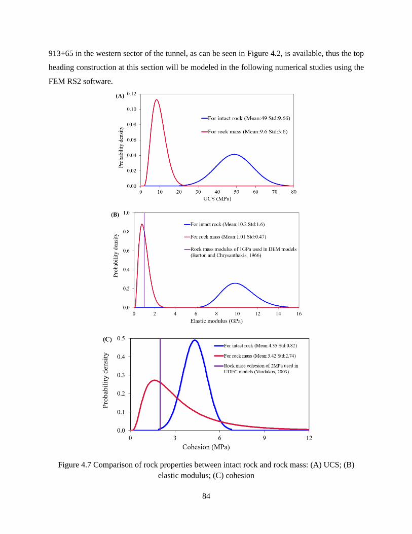
84
913+65 in the western sector of the tunnel, as can be seen in Figure 4.2, is available, thus the top
heading construction at this section will be modeled in the following numerical studies using the
FEM RS2 software.
Figure 4.7 Comparison of rock properties between intact rock and rock mass: (A) UCS; (B)
elastic modulus; (C) cohesion
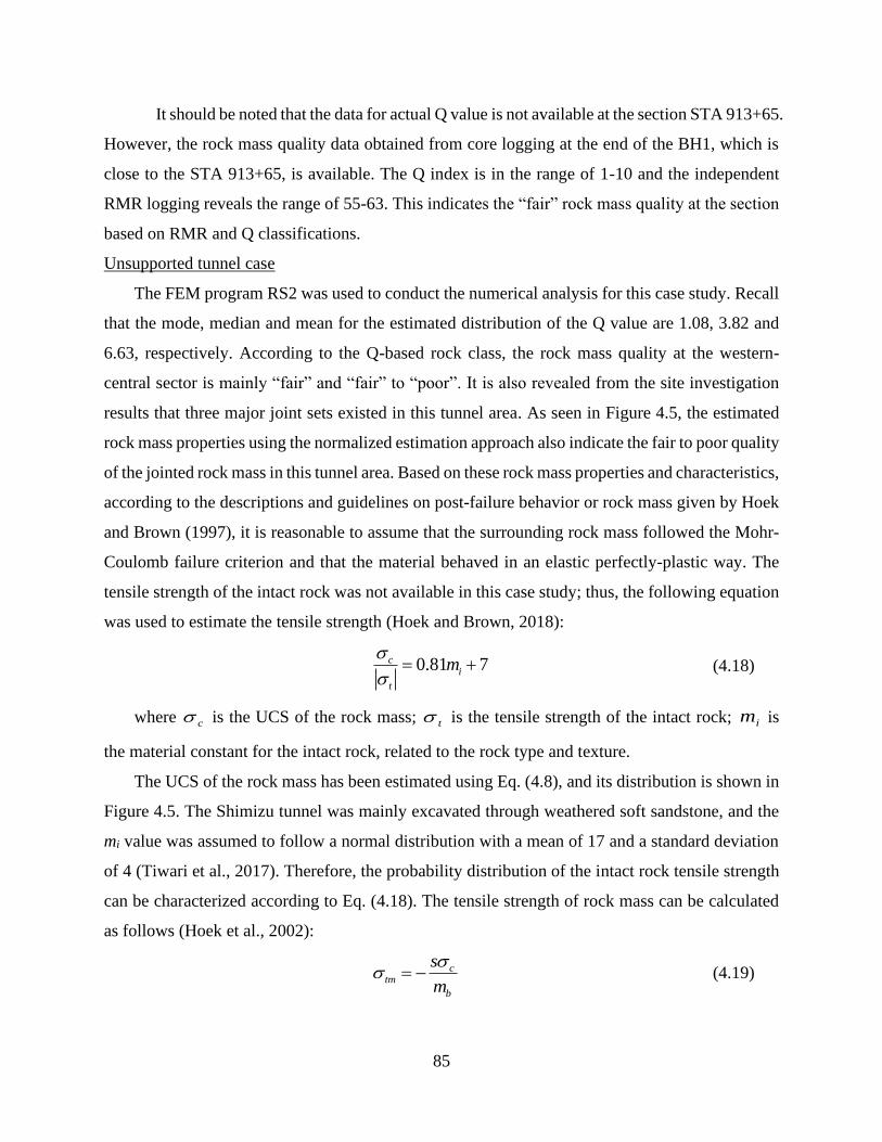
85
It should be noted that the data for actual Q value is not available at the section STA 913+65.
However, the rock mass quality data obtained from core logging at the end of the BH1, which is
close to the STA 913+65, is available. The Q index is in the range of 1-10 and the independent
RMR logging reveals the range of 55-63. This indicates the “fair” rock mass quality at the section
based on RMR and Q classifications.
Unsupported tunnel case
The FEM program RS2 was used to conduct the numerical analysis for this case study. Recall
that the mode, median and mean for the estimated distribution of the Q value are 1.08, 3.82 and
6.63, respectively. According to the Q-based rock class, the rock mass quality at the western-
central sector is mainly “fair” and “fair” to “poor”. It is also revealed from the site investigation
results that three major joint sets existed in this tunnel area. As seen in Figure 4.5, the estimated
rock mass properties using the normalized estimation approach also indicate the fair to poor quality
of the jointed rock mass in this tunnel area. Based on these rock mass properties and characteristics,
according to the descriptions and guidelines on post-failure behavior or rock mass given by Hoek
and Brown (1997), it is reasonable to assume that the surrounding rock mass followed the Mohr-
Coulomb failure criterion and that the material behaved in an elastic perfectly-plastic way. The
tensile strength of the intact rock was not available in this case study; thus, the following equation
was used to estimate the tensile strength (Hoek and Brown, 2018):
0.81 7ci
t
m
= + (4.18)
where c is the UCS of the rock mass; t is the tensile strength of the intact rock; im is
the material constant for the intact rock, related to the rock type and texture.
The UCS of the rock mass has been estimated using Eq. (4.8), and its distribution is shown in
Figure 4.5. The Shimizu tunnel was mainly excavated through weathered soft sandstone, and the
mi value was assumed to follow a normal distribution with a mean of 17 and a standard deviation
of 4 (Tiwari et al., 2017). Therefore, the probability distribution of the intact rock tensile strength
can be characterized according to Eq. (4.18). The tensile strength of rock mass can be calculated
as follows (Hoek et al., 2002):
ctm
b
s
m
= − (4.19)
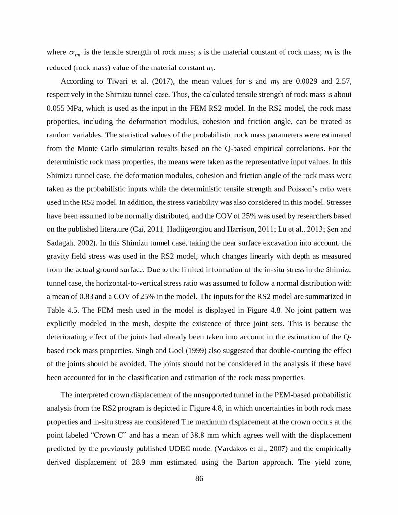
86
where tm is the tensile strength of rock mass; s is the material constant of rock mass; mb is the
reduced (rock mass) value of the material constant mi.
According to Tiwari et al. (2017), the mean values for s and mb are 0.0029 and 2.57,
respectively in the Shimizu tunnel case. Thus, the calculated tensile strength of rock mass is about
0.055 MPa, which is used as the input in the FEM RS2 model. In the RS2 model, the rock mass
properties, including the deformation modulus, cohesion and friction angle, can be treated as
random variables. The statistical values of the probabilistic rock mass parameters were estimated
from the Monte Carlo simulation results based on the Q-based empirical correlations. For the
deterministic rock mass properties, the means were taken as the representative input values. In this
Shimizu tunnel case, the deformation modulus, cohesion and friction angle of the rock mass were
taken as the probabilistic inputs while the deterministic tensile strength and Poisson’s ratio were
used in the RS2 model. In addition, the stress variability was also considered in this model. Stresses
have been assumed to be normally distributed, and the COV of 25% was used by researchers based
on the published literature (Cai, 2011; Hadjigeorgiou and Harrison, 2011; Lü et al., 2013; Şen and
Sadagah, 2002). In this Shimizu tunnel case, taking the near surface excavation into account, the
gravity field stress was used in the RS2 model, which changes linearly with depth as measured
from the actual ground surface. Due to the limited information of the in-situ stress in the Shimizu
tunnel case, the horizontal-to-vertical stress ratio was assumed to follow a normal distribution with
a mean of 0.83 and a COV of 25% in the model. The inputs for the RS2 model are summarized in
Table 4.5. The FEM mesh used in the model is displayed in Figure 4.8. No joint pattern was
explicitly modeled in the mesh, despite the existence of three joint sets. This is because the
deteriorating effect of the joints had already been taken into account in the estimation of the Q-
based rock mass properties. Singh and Goel (1999) also suggested that double-counting the effect
of the joints should be avoided. The joints should not be considered in the analysis if these have
been accounted for in the classification and estimation of the rock mass properties.
The interpreted crown displacement of the unsupported tunnel in the PEM-based probabilistic
analysis from the RS2 program is depicted in Figure 4.8, in which uncertainties in both rock mass
properties and in-situ stress are considered The maximum displacement at the crown occurs at the
point labeled “Crown C” and has a mean of 38.8 mm which agrees well with the displacement
predicted by the previously published UDEC model (Vardakos et al., 2007) and the empirically
derived displacement of 28.9 mm estimated using the Barton approach. The yield zone,
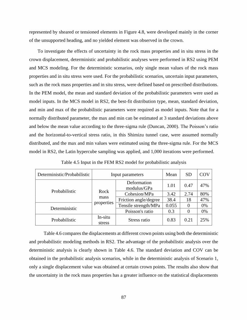
87
represented by sheared or tensioned elements in Figure 4.8, were developed mainly in the corner
of the unsupported heading, and no yielded element was observed in the crown.
To investigate the effects of uncertainty in the rock mass properties and in situ stress in the
crown displacement, deterministic and probabilistic analyses were performed in RS2 using PEM
and MCS modeling. For the deterministic scenarios, only single mean values of the rock mass
properties and in situ stress were used. For the probabilistic scenarios, uncertain input parameters,
such as the rock mass properties and in situ stress, were defined based on prescribed distributions.
In the PEM model, the mean and standard deviation of the probabilistic parameters were used as
model inputs. In the MCS model in RS2, the best-fit distribution type, mean, standard deviation,
and min and max of the probabilistic parameters were required as model inputs. Note that for a
normally distributed parameter, the max and min can be estimated at 3 standard deviations above
and below the mean value according to the three-sigma rule (Duncan, 2000). The Poisson’s ratio
and the horizontal-to-vertical stress ratio, in this Shimizu tunnel case, were assumed normally
distributed, and the max and min values were estimated using the three-sigma rule. For the MCS
model in RS2, the Latin hypercube sampling was applied, and 1,000 iterations were performed.
Table 4.5 Input in the FEM RS2 model for probabilistic analysis
Deterministic/Probabilistic Input parameters Mean SD COV
Probabilistic Rock
mass
properties
Deformation
modulus/GPa 1.01 0.47 47%
Cohesion/MPa 3.42 2.74 80%
Friction angle/degree 38.4 18 47%
Deterministic Tensile strength/MPa 0.055 0 0%
Poisson's ratio 0.3 0 0%
Probabilistic In-situ
stress Stress ratio 0.83 0.21 25%
Table 4.6 compares the displacements at different crown points using both the deterministic
and probabilistic modeling methods in RS2. The advantage of the probabilistic analysis over the
deterministic analysis is clearly shown in Table 4.6. The standard deviation and COV can be
obtained in the probabilistic analysis scenarios, while in the deterministic analysis of Scenario 1,
only a single displacement value was obtained at certain crown points. The results also show that
the uncertainty in the rock mass properties has a greater influence on the statistical displacements
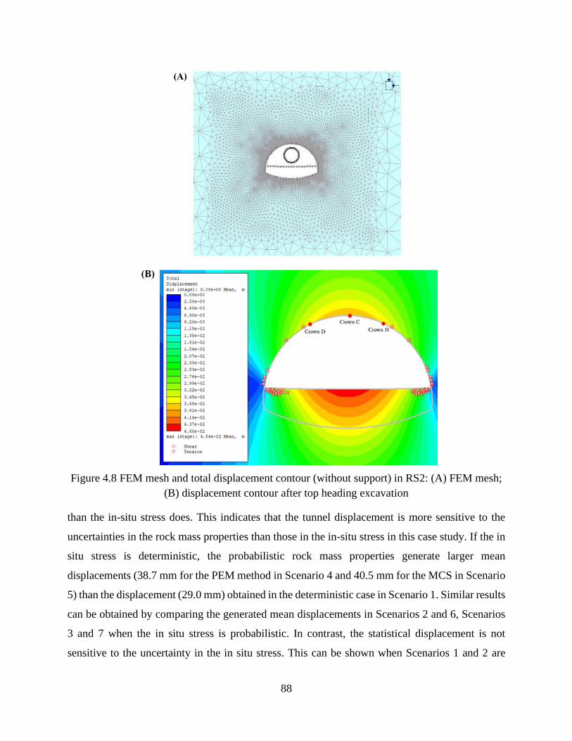
88
Figure 4.8 FEM mesh and total displacement contour (without support) in RS2: (A) FEM mesh;
(B) displacement contour after top heading excavation
than the in-situ stress does. This indicates that the tunnel displacement is more sensitive to the
uncertainties in the rock mass properties than those in the in-situ stress in this case study. If the in
situ stress is deterministic, the probabilistic rock mass properties generate larger mean
displacements (38.7 mm for the PEM method in Scenario 4 and 40.5 mm for the MCS in Scenario
5) than the displacement (29.0 mm) obtained in the deterministic case in Scenario 1. Similar results
can be obtained by comparing the generated mean displacements in Scenarios 2 and 6, Scenarios
3 and 7 when the in situ stress is probabilistic. In contrast, the statistical displacement is not
sensitive to the uncertainty in the in situ stress. This can be shown when Scenarios 1 and 2 are
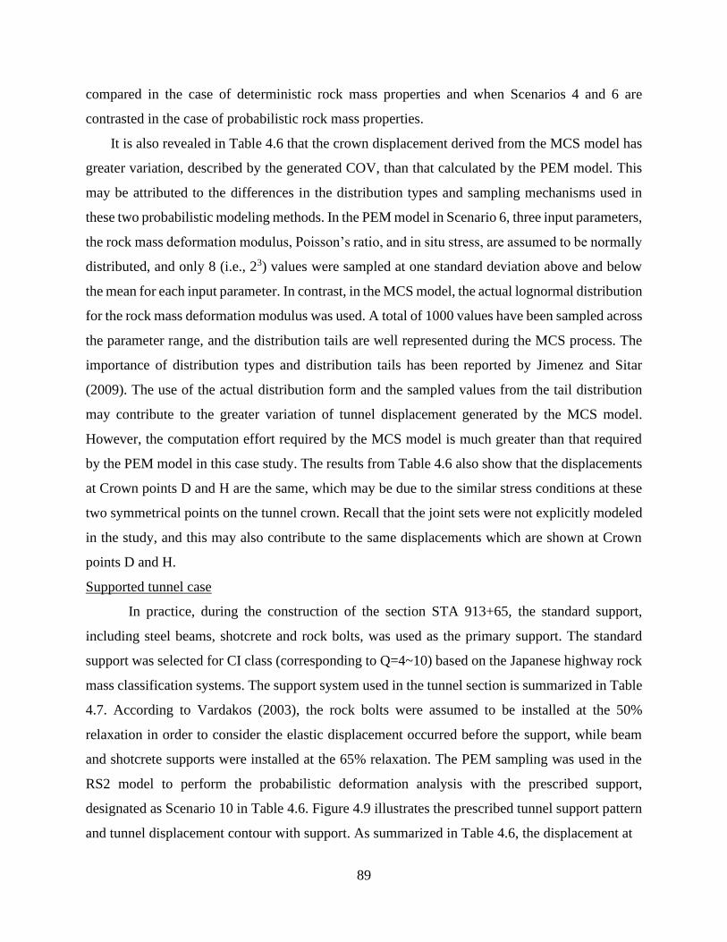
89
compared in the case of deterministic rock mass properties and when Scenarios 4 and 6 are
contrasted in the case of probabilistic rock mass properties.
It is also revealed in Table 4.6 that the crown displacement derived from the MCS model has
greater variation, described by the generated COV, than that calculated by the PEM model. This
may be attributed to the differences in the distribution types and sampling mechanisms used in
these two probabilistic modeling methods. In the PEM model in Scenario 6, three input parameters,
the rock mass deformation modulus, Poisson’s ratio, and in situ stress, are assumed to be normally
distributed, and only 8 (i.e., 23) values were sampled at one standard deviation above and below
the mean for each input parameter. In contrast, in the MCS model, the actual lognormal distribution
for the rock mass deformation modulus was used. A total of 1000 values have been sampled across
the parameter range, and the distribution tails are well represented during the MCS process. The
importance of distribution types and distribution tails has been reported by Jimenez and Sitar
(2009). The use of the actual distribution form and the sampled values from the tail distribution
may contribute to the greater variation of tunnel displacement generated by the MCS model.
However, the computation effort required by the MCS model is much greater than that required
by the PEM model in this case study. The results from Table 4.6 also show that the displacements
at Crown points D and H are the same, which may be due to the similar stress conditions at these
two symmetrical points on the tunnel crown. Recall that the joint sets were not explicitly modeled
in the study, and this may also contribute to the same displacements which are shown at Crown
points D and H.
Supported tunnel case
In practice, during the construction of the section STA 913+65, the standard support,
including steel beams, shotcrete and rock bolts, was used as the primary support. The standard
support was selected for CI class (corresponding to Q=4~10) based on the Japanese highway rock
mass classification systems. The support system used in the tunnel section is summarized in Table
4.7. According to Vardakos (2003), the rock bolts were assumed to be installed at the 50%
relaxation in order to consider the elastic displacement occurred before the support, while beam
and shotcrete supports were installed at the 65% relaxation. The PEM sampling was used in the
RS2 model to perform the probabilistic deformation analysis with the prescribed support,
designated as Scenario 10 in Table 4.6. Figure 4.9 illustrates the prescribed tunnel support pattern
and tunnel displacement contour with support. As summarized in Table 4.6, the displacement at

90
Table 4.6 Summary of tunnel crown displacement in different scenarios
Support
scheme Input parameters
Modeling
Method Scenario
Displacement (mm)
Point C Point D Point H
Numerical
calculation
without
support
Rock mass
properties In-situ stress Mean SD COV Mean SD COV Mean SD COV
Deterministic
Deterministic Deterministic 1 29 0 0 25.1 0 0 25.1 0 0
Probabilistic PEM 2 29 0.98 3% 25.2 0.1 0.4% 25.2 0.1 0.4%
MCS 3 29 0.689 2% 25.2 0.11 0.4% 25.2 0.11 0.4%
Probabilistic
Deterministic PEM 4 38.7 19.6 51% 33.9 17.4 51% 33.9 17.4 51%
MCS 5 40.5 25.1 62% 35.4 21.9 62% 35.4 22.0 62%
Probabilistic PEM 6 38.8 19 49% 34.1 16.9 50% 34.1 16.9 50%
MCS 7 40.5 24.8 61% 35.6 21.9 62% 35.6 21.9 62%
UDEC calculation results by Vardakos et al.,
(2007) 8 30~40 N/A
Empirical results from the Barton approach (Eq. 4.14) 9 28.9 36.9 128% N/A
With
support
Probabilistic Probabilistic PEM 10 19.1 9.08 48% 15.7 7.44 47% 15.7 7.44 47%
Actually measured value 11 11.5 N/A 13 N/A 12 N/A
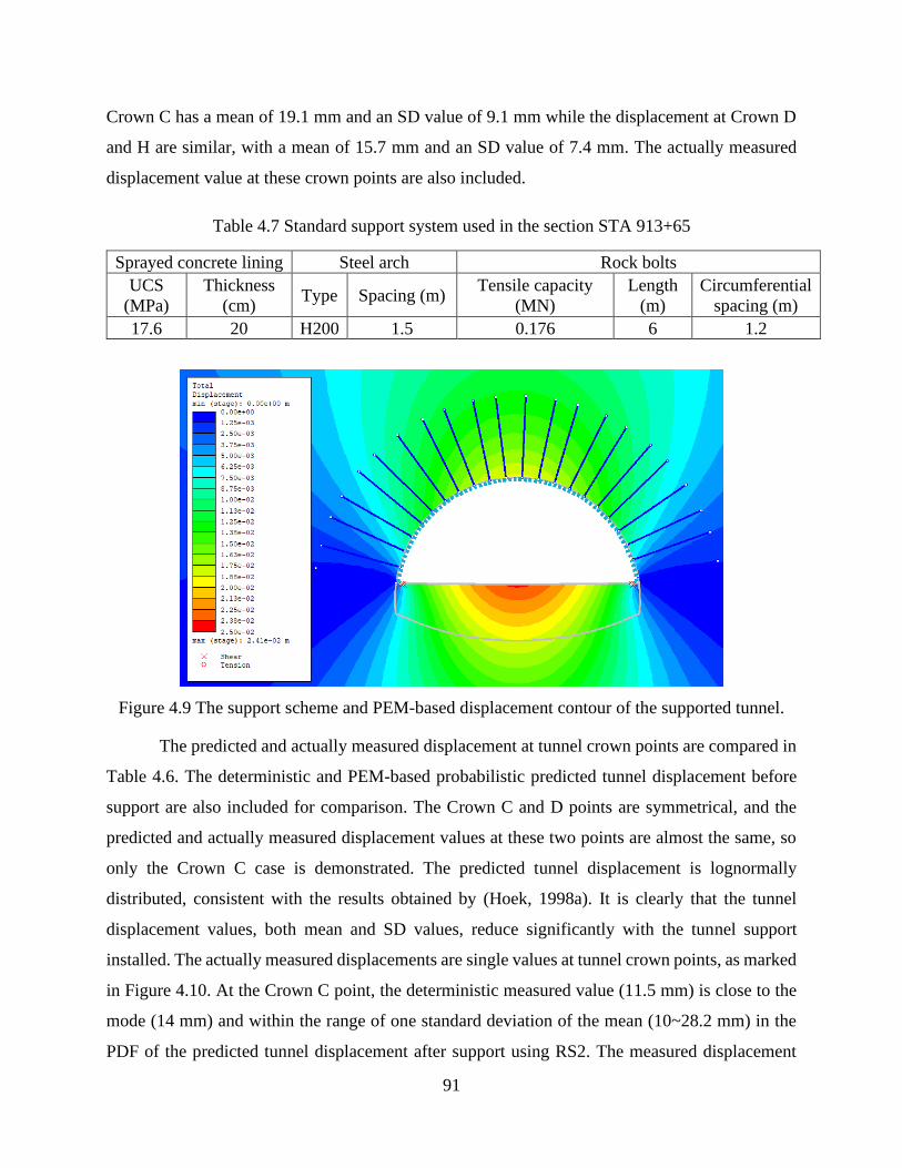
91
Crown C has a mean of 19.1 mm and an SD value of 9.1 mm while the displacement at Crown D
and H are similar, with a mean of 15.7 mm and an SD value of 7.4 mm. The actually measured
displacement value at these crown points are also included.
Table 4.7 Standard support system used in the section STA 913+65
Sprayed concrete lining Steel arch Rock bolts
UCS
(MPa)
Thickness
(cm) Type Spacing (m)
Tensile capacity
(MN)
Length
(m)
Circumferential
spacing (m)
17.6 20 H200 1.5 0.176 6 1.2
Figure 4.9 The support scheme and PEM-based displacement contour of the supported tunnel.
The predicted and actually measured displacement at tunnel crown points are compared in
Table 4.6. The deterministic and PEM-based probabilistic predicted tunnel displacement before
support are also included for comparison. The Crown C and D points are symmetrical, and the
predicted and actually measured displacement values at these two points are almost the same, so
only the Crown C case is demonstrated. The predicted tunnel displacement is lognormally
distributed, consistent with the results obtained by (Hoek, 1998a). It is clearly that the tunnel
displacement values, both mean and SD values, reduce significantly with the tunnel support
installed. The actually measured displacements are single values at tunnel crown points, as marked
in Figure 4.10. At the Crown C point, the deterministic measured value (11.5 mm) is close to the
mode (14 mm) and within the range of one standard deviation of the mean (10~28.2 mm) in the
PDF of the predicted tunnel displacement after support using RS2. The measured displacement
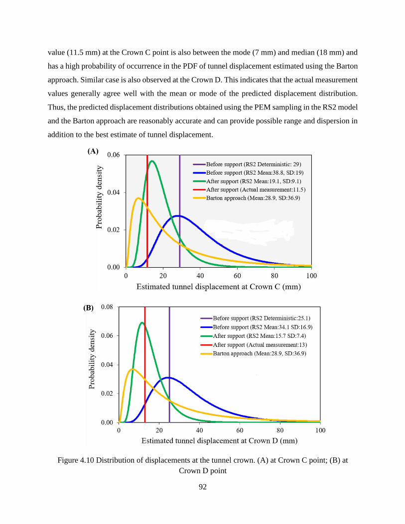
92
value (11.5 mm) at the Crown C point is also between the mode (7 mm) and median (18 mm) and
has a high probability of occurrence in the PDF of tunnel displacement estimated using the Barton
approach. Similar case is also observed at the Crown D. This indicates that the actual measurement
values generally agree well with the mean or mode of the predicted displacement distribution.
Thus, the predicted displacement distributions obtained using the PEM sampling in the RS2 model
and the Barton approach are reasonably accurate and can provide possible range and dispersion in
addition to the best estimate of tunnel displacement.
Figure 4.10 Distribution of displacements at the tunnel crown. (A) at Crown C point; (B) at
Crown D point
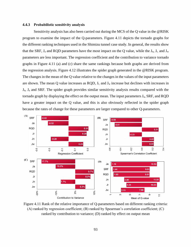
93
4.4.3 Probabilistic sensitivity analysis
Sensitivity analysis has also been carried out during the MCS of the Q value in the @RISK
program to examine the impact of the Q-parameters. Figure 4.11 depicts the tornado graphs for
the different ranking techniques used in the Shimizu tunnel case study. In general, the results show
that the SRF, Ja and RQD parameters have the most impact on the Q value, while the Jn, Jr, and Jw
parameters are less important. The regression coefficient and the contribution to variance tornado
graphs in Figure 4.11 (a) and (c) share the same rankings because both graphs are derived from
the regression analysis. Figure 4.12 illustrates the spider graph generated in the @RISK program.
The changes in the mean of the Q value relative to the changes in the values of the input parameters
are shown. The mean Q value increases as RQD, Jr, and Jw increase but declines with increases in
Jn, Ja and SRF. The spider graph provides similar sensitivity analysis results compared with the
tornado graph by displaying the effect on the output mean. The input parameters Ja, SRF, and RQD
have a greater impact on the Q value, and this is also obviously reflected in the spider graph
because the rates of change for these parameters are larger compared to other Q-parameters.
Figure 4.11 Rank of the relative importance of Q-parameters based on different ranking criteria:
(A) ranked by regression coefficient; (B) ranked by Spearman’s correlation coefficient; (C)
ranked by contribution to variance; (D) ranked by effect on output mean
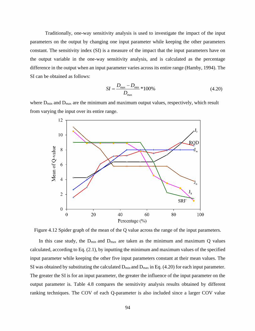
94
Traditionally, one-way sensitivity analysis is used to investigate the impact of the input
parameters on the output by changing one input parameter while keeping the other parameters
constant. The sensitivity index (SI) is a measure of the impact that the input parameters have on
the output variable in the one-way sensitivity analysis, and is calculated as the percentage
difference in the output when an input parameter varies across its entire range (Hamby, 1994). The
SI can be obtained as follows:
max min
max
*100%D D
SID
−= (4.20)
where Dmin and Dmax are the minimum and maximum output values, respectively, which result
from varying the input over its entire range.
Figure 4.12 Spider graph of the mean of the Q value across the range of the input parameters.
In this case study, the Dmin and Dmax are taken as the minimum and maximum Q values
calculated, according to Eq. (2.1), by inputting the minimum and maximum values of the specified
input parameter while keeping the other five input parameters constant at their mean values. The
SI was obtained by substituting the calculated Dmin and Dmax in Eq. (4.20) for each input parameter.
The greater the SI is for an input parameter, the greater the influence of the input parameter on the
output parameter is. Table 4.8 compares the sensitivity analysis results obtained by different
ranking techniques. The COV of each Q-parameter is also included since a larger COV value
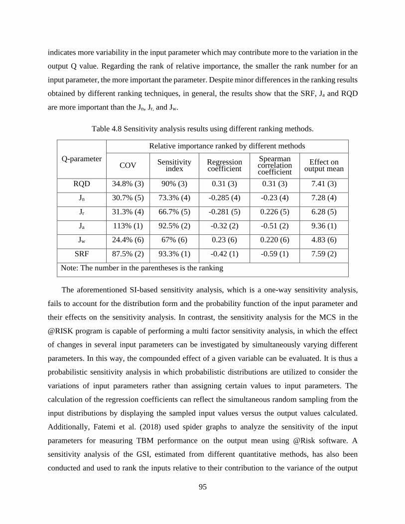
95
indicates more variability in the input parameter which may contribute more to the variation in the
output Q value. Regarding the rank of relative importance, the smaller the rank number for an
input parameter, the more important the parameter. Despite minor differences in the ranking results
obtained by different ranking techniques, in general, the results show that the SRF, Ja and RQD
are more important than the Jn, Jr, and Jw.
Table 4.8 Sensitivity analysis results using different ranking methods.
Q-parameter
Relative importance ranked by different methods
COV Sensitivity index
Regression coefficient
Spearman correlation coefficient
Effect on output mean
RQD 34.8% (3) 90% (3) 0.31 (3) 0.31 (3) 7.41 (3)
Jn 30.7% (5) 73.3% (4) -0.285 (4) -0.23 (4) 7.28 (4)
Jr 31.3% (4) 66.7% (5) -0.281 (5) 0.226 (5) 6.28 (5)
Ja 113% (1) 92.5% (2) -0.32 (2) -0.51 (2) 9.36 (1)
Jw 24.4% (6) 67% (6) 0.23 (6) 0.220 (6) 4.83 (6)
SRF 87.5% (2) 93.3% (1) -0.42 (1) -0.59 (1) 7.59 (2)
Note: The number in the parentheses is the ranking
The aforementioned SI-based sensitivity analysis, which is a one-way sensitivity analysis,
fails to account for the distribution form and the probability function of the input parameter and
their effects on the sensitivity analysis. In contrast, the sensitivity analysis for the MCS in the
@RISK program is capable of performing a multi factor sensitivity analysis, in which the effect
of changes in several input parameters can be investigated by simultaneously varying different
parameters. In this way, the compounded effect of a given variable can be evaluated. It is thus a
probabilistic sensitivity analysis in which probabilistic distributions are utilized to consider the
variations of input parameters rather than assigning certain values to input parameters. The
calculation of the regression coefficients can reflect the simultaneous random sampling from the
input distributions by displaying the sampled input values versus the output values calculated.
Additionally, Fatemi et al. (2018) used spider graphs to analyze the sensitivity of the input
parameters for measuring TBM performance on the output mean using @Risk software. A
sensitivity analysis of the GSI, estimated from different quantitative methods, has also been
conducted and used to rank the inputs relative to their contribution to the variance of the output
96
(Morelli, 2015). In a rock tunnel case study, the probabilistic input parameters in the Q-system
were also ranked by their effect on the output mean, regression coefficient, Spearman correlation
coefficient and contribution to variance using the @RISK program (Lu et al., 2018a).
A sensitivity analysis is a useful tool to characterize the relationship between the input
parameters and the output parameters as well as identify the most influential input parameters.
However, in ground characterization and rock mass classification, sensitivity analyses of
geological parameters are not adequately conducted. Instead, it is often assumed that all the
geological parameters are equally important, which obviously fails to realistically assess the
different impact that input parameters have on output parameters. Thus, it is essential to perform
sensitivity analyses on ground parameters in the site investigation stage, especially for complex
and challenging ground conditions. It is also beneficial to know which input parameter is the most
influential overall to the rock mass quality, so that precautionary measures (e.g., dewatering,
grouting, freezing, pre-blasting) can be taken in advance to improve the rock mass quality before
excavation. The different ranking techniques in the sensitivity analysis can be used for comparative
and checking purposes.
4.4.4 Effects of the correlation between the RQD and Jn
The effect of the negative correlation between the RQD and Jn on the Q value, rock mass
properties and the displacement estimated by the Barton approach is shown in Table 4.9. In general,
the stronger the negative correlation is between the RQD and Jn, the greater the mean and the
variation are, as described by the calculated COV of the output parameters. Wang and Akeju (2016)
also reported that the output would be affected to a greater degree by the combination of correlated
input parameters. The mean and range of the Q value, rock mass properties and displacement may
be underestimated if the negative correlation is not taken into account. The SI was also calculated
according to Eq. (4.20) to investigate the sensitivity of the mean and COV of the output parameters
to the correlation coefficient, as displayed in the last row in Table 4.9. Regarding the sensitivity
indices for all the output parameters, the SI for the displacement is the largest, followed by the SI
for cohesion and the Q value, with the smallest SI being that for the deformation modulus and the
UCS. This demonstrates that the negative correlation between the RQD and Jn has a greater impact
on the displacement, cohesion and the Q value than on the deformation modulus and the UCS.
This is related to the empirical correlations on which the output parameters are calculated, as
shown in Table 4.1. For example, the displacement estimated by the Barton approach is associated
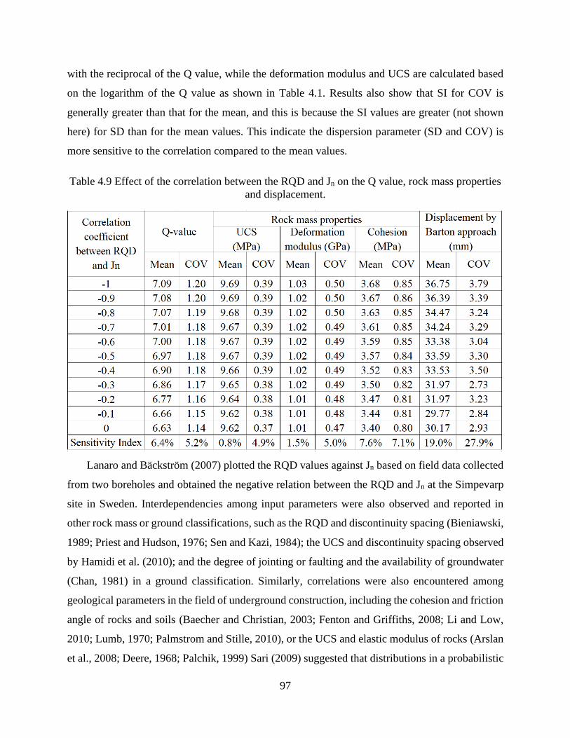
97
with the reciprocal of the Q value, while the deformation modulus and UCS are calculated based
on the logarithm of the Q value as shown in Table 4.1. Results also show that SI for COV is
generally greater than that for the mean, and this is because the SI values are greater (not shown
here) for SD than for the mean values. This indicate the dispersion parameter (SD and COV) is
more sensitive to the correlation compared to the mean values.
Table 4.9 Effect of the correlation between the RQD and Jn on the Q value, rock mass properties
and displacement.
Lanaro and Bäckström (2007) plotted the RQD values against Jn based on field data collected
from two boreholes and obtained the negative relation between the RQD and Jn at the Simpevarp
site in Sweden. Interdependencies among input parameters were also observed and reported in
other rock mass or ground classifications, such as the RQD and discontinuity spacing (Bieniawski,
1989; Priest and Hudson, 1976; Sen and Kazi, 1984); the UCS and discontinuity spacing observed
by Hamidi et al. (2010); and the degree of jointing or faulting and the availability of groundwater
(Chan, 1981) in a ground classification. Similarly, correlations were also encountered among
geological parameters in the field of underground construction, including the cohesion and friction
angle of rocks and soils (Baecher and Christian, 2003; Fenton and Griffiths, 2008; Li and Low,
2010; Lumb, 1970; Palmstrom and Stille, 2010), or the UCS and elastic modulus of rocks (Arslan
et al., 2008; Deere, 1968; Palchik, 1999) Sari (2009) suggested that distributions in a probabilistic
98
model will often have to be correlated to ensure that only meaningful scenarios are generated
during the model’s iterations. For example, a weathered discontinuity may have a wider opening,
while a strong rock is expected to have a narrower aperture (Sari, 2009). Leu and Adi (2011) also
proposed that it is more realistic to correlate geological parameters in ground classification because
one parameter may depend on the status of the other parameters.
Unfortunately, few studies have focused on the correlation among input parameters in rock
mass or ground classification. The interdependencies among ground parameters are mostly
overlooked, and it is assumed that all the input parameters are independent. However,
dependencies among ground parameters can be critical to obtaining proper numerical results in
engineering practice, particularly in probabilistic assessments and reliability analyses of
geotechnical structures (Baecher and Christian, 2003; Wang and Akeju, 2016; Wang and Aladejare,
2016). The significant effect of correlations between ground parameters on a reliability analysis
and probabilistic design in underground construction has been highlighted (Li and Low, 2010; Lü
and Low, 2011; Lü et al., 2011). If the correlation between input parameters in a probabilistic
analysis is neglected, the estimated probability of failure may be severely underestimated or
overestimated and might differ by orders of magnitude (Lü et al., 2012; Wang and Aladejare, 2016).
Therefore, it is advisable to account for and appropriately quantify the negative correlation
between the RQD and Jn in estimating the probability distribution of the Q value.
4.4.5 Effects of distribution types of Q-parameters
To investigate the effect of the Q-parameters distribution types on the Q value and
associated output parameters, different commonly used distribution types have been assigned,
based on the relative frequency histogram in Scenario 1, to each Q-parameter. The uniform
distribution in Scenario 2, also called the “noninformative priors” distribution, is commonly used
when the available information is vague and only the bounds of the parameter are given. This
distribution was also used to model all the input parameters in this case. The truncated triangular
distribution, for which the typical range definition is adopted from Barton et al. (1974), is used in
Scenario 15 and was also used to model each Q-parameter. The minimum and maximum values
of the actual histogram data were used as the truncated values. Panthi (2006) used the truncated
triangular distribution for the Q-parameters to simulate the rock mass quality Q in tunnels in
regions of the Himalayas. In Scenario 16, the best fitting distributions relative to the histogram
data for all the Q-parameters were obtained using the distribution fit function in the @RISK
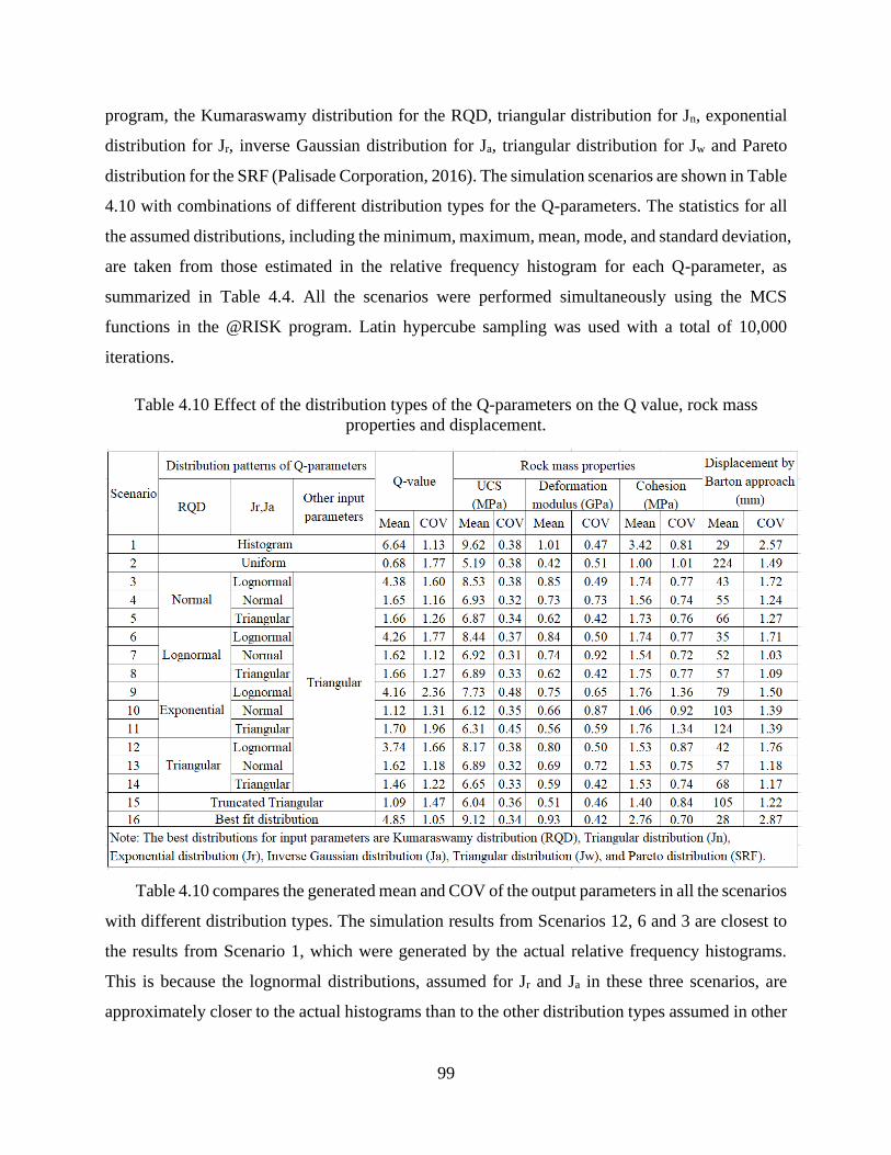
99
program, the Kumaraswamy distribution for the RQD, triangular distribution for Jn, exponential
distribution for Jr, inverse Gaussian distribution for Ja, triangular distribution for Jw and Pareto
distribution for the SRF (Palisade Corporation, 2016). The simulation scenarios are shown in Table
4.10 with combinations of different distribution types for the Q-parameters. The statistics for all
the assumed distributions, including the minimum, maximum, mean, mode, and standard deviation,
are taken from those estimated in the relative frequency histogram for each Q-parameter, as
summarized in Table 4.4. All the scenarios were performed simultaneously using the MCS
functions in the @RISK program. Latin hypercube sampling was used with a total of 10,000
iterations.
Table 4.10 Effect of the distribution types of the Q-parameters on the Q value, rock mass
properties and displacement.
Table 4.10 compares the generated mean and COV of the output parameters in all the scenarios
with different distribution types. The simulation results from Scenarios 12, 6 and 3 are closest to
the results from Scenario 1, which were generated by the actual relative frequency histograms.
This is because the lognormal distributions, assumed for Jr and Ja in these three scenarios, are
approximately closer to the actual histograms than to the other distribution types assumed in other
100
simulation scenarios. Although the best fit for Jr and Ja is an exponential distribution and an inverse
Gaussian distribution, respectively, the lognormal distribution also captures the distribution
characteristics of Jr and Ja, as shown in Figure 4.3 (c) and (d). Comparing the results generated in
Scenarios 3, 6, 9 and 12, in which Jr and Ja are assumed to be lognormally distributed, the triangular
distribution assumption for RQD in Scenario 12 performed best. This is because the distribution
of the RQD is negatively skewed, as shown in Figure 4.3 (a), and the negatively skewed triangular
distribution can better capture this type of data than the normal or lognormal distribution can.
Barton and Grimstad (2014) stated that a lognormally distributed RQD with positive skewness is
commonly found in “very poor” rock masses with a Q-range of 0.1−1, while a normally distributed
RQD is found in “poor” rock masses with a Q-range of 1−4 and a negatively skewed RQD
distribution is found in “fair” to “good” rock masses with a Q-range of 4−40. In the Shimizu case
study, the average rock mass quality is “fair” with a mean value of 6.63, and the negatively skewed
triangular RQD distribution in Scenario 12 matches better with the actual relative frequency
histogram in Figure 4.3(a) than does the positively skewed lognormal distribution in Scenario 6 or
the normal distribution in Scenario 3. It is also shown that in Scenario 2, in which all the input
parameters are assumed to be uniformly distributed, a much smaller mean and a larger COV is
generated than in Scenario 1. This demonstrates that Scenario 2, with a uniform distribution
assumption, provides a greatly underestimated mean value with a larger variation. The triangular
distribution without truncation in Scenario 14 achieves better results than the triangular
distribution with truncations in Scenario 15. The best fit distribution used in Scenario 16 generates
results closest to those generated from the actual relative frequency histograms of all the simulation
scenarios used in Scenario 1. Thus, it is desirable to assign an appropriate distribution (e.g., best
fit distribution) to each input parameter to generate more realistic results for the output parameters.
If a theoretical distribution is well fitted to the empirical frequency data (e.g., the relative
frequency histogram), then random samples can be drawn from the fitted distribution in the MCS
(Fenton and Griffiths, 2008). A continuous probability distribution function, which has a scientific
rationale and is mathematically or computationally tractable, is a useful tool in probabilistic risk
analysis for addressing uncertainties and making informed decisions. The advantages of a
probability distribution function over a relative frequency histogram are summarized by Fenton
and Griffiths (2008): first, the irregularities, commonly encountered in the histogram due to a finite
amount of sampled data, are smoothed by fitting a continuous distribution; second, the fitted
101
distribution can produce values outside the range of the finite sampled data, meaning that the
effects of extreme values can also be taken into account; third, the fitted distribution has descriptive
statistical parameters while the detailed fluctuations in a histogram will change if the interval sizes
are changed; most notably, the fitted distribution also enables making estimations of stochastic
model parameters and drawing inferences, which allows one to make probabilistic inferential
statements for an entire site where data are limited or not available.
If sufficient data are available, the distribution that best fits the histogram of the data should
be selected. However, in rock engineering the subsurface information is often scarce, and only a
limited number of samples in limited regions are used for estimating the rock mass quality in the
site investigation stage (Fenton and Griffiths, 2008; Langford, 2013). Thus, it may be difficult or
inappropriate to obtain the best fit distribution for such insufficient and incomplete frequency data.
Fortunately, certain probability distribution models are found to be suitable for explicitly modeling
the uncertainty or variability in some geological parameters, as reported by previous studies in the
geotechnical literature (Adoko et al., 2013). For example, probabilistic models such as the normal,
lognormal and beta distributions have been successfully utilized to describe the variability in rock
and soil properties, including the UCS, elastic modulus, cohesion and friction angle based on an
extensive literature review and case studies (Ang and Tang, 2007; Baecher and Christian, 2003;
Fenton and Griffiths, 2008; Hoek, 1998a; Lacasse and Nadim, 1996; Lumb, 1970; Phoon and
Kulhawy, 1999). Therefore, it is advisable to properly assume certain probability distribution types
for the input parameters in the Q-system to realistically estimate the probability distribution of the
Q value based on published literature and empirical experience. Additionally, the selected
distributions should be as simple as possible while still reflecting the basic nature of the variability
(Fenton and Griffiths, 2008). In the Shimizu study, the best fit for the RQD is the Kumaraswamy
distribution, a Beta-like distribution, but it is not commonly used in geotechnical engineering.
Instead, a negatively skewed triangular distribution, despite not being the best fit, matches the
histogram data of the RQD well and can be used as an alternative. The triangular distribution of
the RQD also generates similar results those of the best fit distribution.
4.5 Conclusions
An MCS-based uncertainty analysis framework for the Q-system has been developed to
probabilistically assess the uncertainty in the Q-parameters and its effect on the Q value and
102
associated rock mass parameters. A case study of the Shimizu highway tunnel was adopted to
implement the proposed framework. Based on the analysis and discussion of the obtained results,
it is concluded that the MCS-based probabilistic analysis allows for the quantitative
characterization of uncertainty and variability in the input parameters and its impact on the output
parameters. The probabilistic distribution of the Q value was obtained with the MCS technique
based on relative frequency histograms of the input parameters. The MCS-derived Q statistics are
more reasonable than the conventional estimation results using the interval analysis. The former
can more realistically take into account the correlations in input parameters in the estimation as
well as providing the full probabilistic distribution of the Q value, while the estimation in the latter
approach is based on assumptions of perfect correlations which are rarely met in practice. Based
on the empirical correlations between rock mass parameters and the Q value, probabilistic
estimates of the rock mass parameters can be obtained, which can also be used as inputs to
numerical models for stress analysis and stability assessment. Caution should be exercised when
selecting appropriate empirical correlations during the probabilistic calculation process. In this
case study, the empirically estimated probabilistic tunnel displacement, obtained by the Barton
approach, generally agreed well with that generated from the probabilistic analysis of the FEM
RS2 numerical model with the PEM and MCS sampling techniques.
In addition, the results of the uncertainty analysis of the probabilistic Q-system suggest that
the probabilistic sensitivity analysis provides a quantitative ranking of the impact of the input
distributions of Q-parameters on the Q value. Different from traditional one-way sensitivity
analysis, the probabilistic sensitivity analysis is a multi-factor analysis technique, in which the
distributions of input parameters are taken into account and simultaneous variations of all the input
parameters are allowed. Probabilistic sensitivity analysis results obtained in the MCS process
generally agreed well with those derived from other sensitivity analysis techniques in this case
study; the mean and variation of the Q value and the associated rock mass parameters have been
underestimated if the negative correlation is not modeled in this case study. For the probabilistic
assessment of the Q value and associated rock mass parameters, it is advisable to select appropriate
distribution types for uncertain Q-parameters when insufficient input parameter data are available.
The selection of proper distributions for input parameters is vital and should be conducted by
combining site knowledge, local experience, and professional judgment.

103
The proposed framework of the MCS-based uncertainty analysis in the probabilistic Q-system
provides an approach for systematically assessing the uncertainty in the rock mass quality and its
propagation to rock mass characterization and ground response evaluation by applying the MCS
technique with appropriate empirical correlations. The probabilistic sensitivity analysis in the
MCS process can also be performed to identify the most influential input parameters in conjunction
with traditional one-way sensitivity analysis techniques. The framework are helpful in providing
insightful information for the probabilistic evaluation of ground responses and rock support
performance of underground structures.
104
CHAPTER 5
RELIABILITY EVALUATION OF STABILITY FOR UNDERGROUND EXCAVATIONS
USING AN EMPIRICAL APPROACH
5.1 Abstract
The critical strain concept has been widely used in analytical or numerical approaches to
evaluate the stability of underground excavations with a strain-based failure criterion. However,
analytical solutions are often based on simplistic assumptions and numerical procedures are
generally computationally expensive, in which deterministic critical strain values are often used.
To address this issue, reliability assessment using an empirical approach has been performed for
the preliminary evaluation on the excavation stability with the First Order Reliability Method
(FORM) algorithm. The probabilistic critical strain, which takes into account uncertainties in rock
mass parameters, and the tunnel strain empirically estimated based on the rock mass classification
Q index were incorporated in the limit state function for reliability evaluation. Monte Carlo
simulation was also conducted for comparing the reliability analysis results with that derived from
the FORM algorithm. A highway tunnel case study was utilized as an example to perform
reliability evaluation on the excavation stability. The probabilistic sensitivity analysis has been
carried out to identify the most influential parameter. The effects of the correlation, distribution
types and coefficient of variation in input parameters on the reliability have also been investigated.
The reliability analysis results show that the tunnel is not expected to experience instability after
excavation. The excavation stability has also been evaluated using analytical and numerical
approaches, and obtained results were consistent with that derived from the reliability assessment,
which has also verified the effectiveness of the reliability-based evaluation on excavation stability
using the empirical approach. Thus, reliability assessment using the FORM algorithm with the Q-
based empirical approach can be used as a complement to analytical and numerical approaches for
the preliminary evaluation of the stability of underground excavations.
5.2 Introduction
Uncertainty is inevitable in engineering geology, and inherent uncertainty in geologic
conditions and geotechnical parameters plays a key role in the field of geotechnical engineering,
including the construction of underground structures. Evaluation and consideration of uncertainty
105
have becoming an increasingly important part in the engineering design and construction (Einstein
and Baecher, 1982). However, traditional deterministic design methods inadequately deal with the
inherent uncertainty and variability, and this may result in over- or under-design of underground
structures and associated risks. For example, in the traditional allowable stress design (ASD)
approach, only the expected case is discussed and an overall margin of safety is applied. The ASD
also does not consider the effects of actual variabilities in load and strength and insufficiently
provides the level of site understanding on the probability of failure (Fenton and Griffiths, 2008).
Fortunately, a more quantitative and systemic approach with the use of probability, statistics and
reliability can provide rational analysis of uncertainty and complement the traditional deterministic
approaches (Einstein and Baecher, 1982).
Reliability assessment represents a rational method to describe design risks by directly
quantifying uncertainties in input parameters in the design process (Langford, 2013). It is capable
of systematically quantifying safety risks and is regarded as a useful tool in solving challenging
geotechnical engineering problems subjected to inherent uncertainty and variability (Zhang and
Goh, 2018). Reliability approaches also provide a more consistent and complete measure of the
risk level since they not only consider the expected case but also offer a measure of design
performance based on the reliability index or probability of failure (Langford, 2013). Reliability-
based design approaches, including the load resistance factor design within a probabilistic
framework, have been widely used in evaluating the reliability and risk level in geotechnical
engineering. Despite its benefits, the reliability analysis in the geotechnical engineering field has
been focused on surface and gravity-driven geotechnical projects where loads and resistances can
be dealt with separately. It has not yet achieved widespread use in the design of underground
construction, and this is attributed to the complex ground-support interaction since the system
performance is dependent on interdependency among rock loads, deformation and support
resistance (Langford, 2013). The load and resistance are difficult to differentiate in underground
construction since the rock mass itself both acts both as the load and support resistance. Thus, it is
not appropriate to independently separate the loads and resistances in underground construction in
a performance function, which is often used to define the acceptance criterion for the system
performance. Instead, the limit state function that is defined with respect to a limiting value for
rock mass response is generally taken as the performance function. Accordingly, the probability
106
of failure, which refers to the violation of the limit state, can be calculated as the likelihood of
exceeding of a prescribed limit state.
The limit states with regard to the stability evaluation of underground structures can be mainly
described by the stress-based failure criteria and strain-based failure criteria. As for the stress-
based failure criteria, Li (1990) stated that the in-situ stresses are generally not directly measurable
and are converted from the displacement or strain through behavior equations. It was also pointed
out that the conversion is normally based on assumptions such as the plane stress condition and
Hooke’s law, which rarely represents actual in-situ conditions and rock mass properties. In
addition, the strength parameters of rock masses in the stress-based failure criteria are often
difficult to obtain since the in-situ tests are expensive and time-consuming (Hoek, 2007). Moreover,
Sakurai (2017) presented that the stress-based yielding criteria, which are used in elasto-plastic
analysis for stability assessment of geo-structures, lead to calculated stress levels that never go
beyond the yield point. As a result, the stress keeps constant while the strain increase beyond the
yielding point till failure, which implies the failure criteria to some extent should be defined in
terms of strain. It is also stated that the apparent factor of safety, defined in terms of stress, will
always be one as the stress state in a plastic zone cannot exceed the yield stress point. In these
scenarios, however, tunnels may still be adequately stable as the plastic zone or failure region is
always surrounded by stable elastic zone (Sakurai, 2017). In contrast, the advantages of strain-
based failure criteria have been summarized over the stress-based failure criteria (Gaede et al.,
2014): the consideration of both elastic and inelastic strain, the direct and observable effects
instead of inferred effects, and the ability of modeling complete stress-strain curves. The
displacement or percent strain is also more practical and easier to measure in underground
construction. Based on these reasons, strain-based failure criteria are of particular interests and
have been widely applied in the underground design and construction (Daraei and Zare, 2018; Fujii
et al., 1998; Hoek, 1998b; Li and Villaescusa, 2005; Li et al., 2000; Li, 1990; Sakurai, 1981; Singh
et al., 2007; Stacey, 1981).
In recent decades, numerous researchers have employed limit state functions with strain-based
failure criteria using the First Order Reliability Method (FORM) or Monte Carlo simulation (MCS)
techniques to evaluate the reliability of underground excavations, and productive results have been
achieved (Li and Low, 2010; Liu and Low, 2017; Lü et al., 2012; Lü and Low, 2011; Lü et al.,
2011; Song et al., 2016). Among these reliability evaluations, analytical expressions based on the
107
ground-support interaction in circular tunnels were used to construct the performance function (Li
and Low, 2010; Su et al., 2011). However, the analytical solution was basically derived with
assumptions of a circular tunnel in isotropic and homogeneous ground subjected to hydrostatic
stress with uniform internal support pressure. These assumed conditions in the analytical solution
are ideal and seldom met in the practice of underground excavation. Alternatively, numerical
procedures with finite element or finite difference models using different algorithms were
developed to implicitly approximate the strain-based performance function for the tunnel
reliability assessment, including the response surface method (RSM) (Hamrouni et al., 2017; Lü
and Low, 2011; Lü et al., 2011; Mollon et al., 2009b, 2010), Regression Method (Basarir, 2008;
Goh and Zhang, 2012; Zhang and Goh, 2015; Zhang and Goh, 2012; Zhu et al., 2008), Artificial
Neural Network (Adoko et al., 2013; Goh and Zhang, 2012; Lü et al., 2012; Mahdevari and Torabi,
2012; Rafiai and Moosavi, 2012), Support Vector Machine (Tan et al., 2011; Zhao, 2008; Zhao et
al., 2014) and Augmented Radial Basis Function (Bai et al., 2012; Fang et al., 2005; Wang et al.,
2016). Reliability approaches, including the First Order Second Moment method, Point Estimate
Method, FORM and MCS techniques, have been used to perform reliability analysis based on
these implicitly constructed performance functions with satisfactory results achieved. It should be
noted, however, that the numerical procedures are generally computationally expensive, which
requires a great number of numerical experimentations or iterations. Actually, in addition to the
analytically or numerically derived performance functions, there are some empirical correlations
related to the displacement or percent strain based on collected case histories of underground
excavations (Barton, 2002; Barton et al., 1994; Chern et al., 1998a; Chern et al., 1998b; Hoek,
1999; Hoek, 2001; Sakurai, 1983) which are useful in the preliminary evaluation of excavation
stability. Nevertheless, few attempts have been made to adopt the empirically derived performance
function with the strain-based failure criterion to assess the reliability and risk levels of
underground excavations. In addition, in regard to reliability evaluations using both the simplistic
analytical solution and sophisticated numerical procedures, as mentioned above, the focus was
primarily the illustration of proposed analysis approaches or numerical algorithms, and
hypothetical examples with assumed statistical moments of rock mass parameters were mostly
used. In other words, few case studies with real statistical data of rock mass properties have been
utilized to verify the validity of proposed approaches or algorithms. Moreover, single deterministic
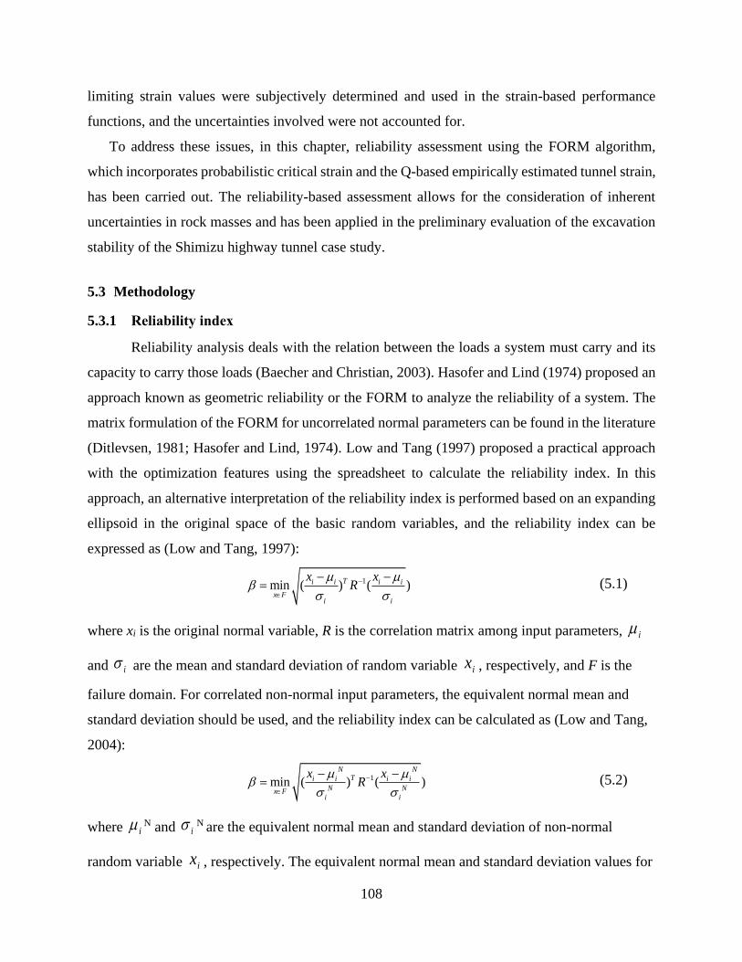
108
limiting strain values were subjectively determined and used in the strain-based performance
functions, and the uncertainties involved were not accounted for.
To address these issues, in this chapter, reliability assessment using the FORM algorithm,
which incorporates probabilistic critical strain and the Q-based empirically estimated tunnel strain,
has been carried out. The reliability-based assessment allows for the consideration of inherent
uncertainties in rock masses and has been applied in the preliminary evaluation of the excavation
stability of the Shimizu highway tunnel case study.
5.3 Methodology
5.3.1 Reliability index
Reliability analysis deals with the relation between the loads a system must carry and its
capacity to carry those loads (Baecher and Christian, 2003). Hasofer and Lind (1974) proposed an
approach known as geometric reliability or the FORM to analyze the reliability of a system. The
matrix formulation of the FORM for uncorrelated normal parameters can be found in the literature
(Ditlevsen, 1981; Hasofer and Lind, 1974). Low and Tang (1997) proposed a practical approach
with the optimization features using the spreadsheet to calculate the reliability index. In this
approach, an alternative interpretation of the reliability index is performed based on an expanding
ellipsoid in the original space of the basic random variables, and the reliability index can be
expressed as (Low and Tang, 1997):
1min ( ) ( )Ti i i i
x Fi i
x xR
−
− −= (5.1)
where xi is the original normal variable, R is the correlation matrix among input parameters, i
and i are the mean and standard deviation of random variable ix , respectively, and F is the
failure domain. For correlated non-normal input parameters, the equivalent normal mean and
standard deviation should be used, and the reliability index can be calculated as (Low and Tang,
2004):
1min ( ) ( )N N
Ti i i i
N Nx Fi i
x xR
−
− −= (5.2)
where i N and i N are the equivalent normal mean and standard deviation of non-normal
random variable ix , respectively. The equivalent normal mean and standard deviation values for

109
non-normal random variables can be computed using the Rackwitz and Flessler (1978) two-
parameter equivalent normal transformation or other transformation techniques.
In the framework of the FORM algorithm using the spreadsheet, the design point is a point
on the boundary (the limit state surface) that separates safe combinations of parametric values from
the unsafe combinations. The design point is the most probable failure combination of parametric
values (Low, 2008b). In reliability analysis using FORM, the uncertainties and correlation
structure of the parameters are represented by a one-standard deviation dispersion ellipsoid
centered at the mean-value point, as shown in Figure 5.1. The safety is expressed by a reliability
index which is the shortest distance (measured in units of directional standard deviations, R/r) from
the mean-value point to the most probable failure combination of parameters (“the design point”)
on the limit state surface (Low, 2018; Low, 2008b). For more information about the constrained
optimization approach from the ellipsoidal perspective, the literature (Low, 2018; Low and Tang,
1997, 2007; Low, 2008b; Low and Tang, 2004) can be referred to. Based on the reliability index,
the probability of failure can be evaluated by (Baecher and Christian, 2003):
1 ( )fp − (5.3)
where fp is the probability of failure, ( ) is the cumulative distribution function of the standard
normal variable.
Figure 5.1 Design point and equivalent ellipsoids (modified from Low and Tang, 2004)
110
A new efficient spreadsheet algorithm for the FORM was proposed and expressed as
follows (Low and Tang, 2007):
1min [ ] [ ]T
x Fn R n −
= (5.4)
1[ ( )]N
i ii iN
i
xn F x
−−= = (5.5)
where n is a column vector of ni; when the value of ni is varied during the constrained optimization,
the corresponding value of xi is automatically calculated; F is the non-normal cumulative
probability distribution at xi; ( in ) is the cumulative distribution function of the standard normal
variable ni.
The reliability index as expressed in Eq. (5.4) can be calculated using the FORM algorithm
by the Excel’s built-in optimization routine “Solver”, subjected to the constraint that the
performance function G(X)=0, where the x values are calculated from Eq. (5.4), and by
automatically changing the values of ni.
5.3.2 Reliability analysis with the critical strain-based limit state function
The implementation procedures of the critical strain-based reliability analysis of the tunnel
using the FORM algorithm are shown as follows:
(1) Establish critical strain-based limit state function
The estimated strain is a function of the Q value using the Barton (2002) estimation
approach. Thus, the limit state function can be expressed as follows:
( ) ( )CG X Q = − (5.6)
0( ) C vG X R= − (5.7)
100
vv
ci
SPAN
Q
= (5.8)
0( )100
vC
ci
SPANG X R
Q
= − (5.9)
where G(X) is the performance function of the system, C is the critical strain; v is the vertical
displacement (in units of mm); SPAN is the tunnel span (in units of mm); v is the vertical stress;
ci is the uniaxial compressive strength of intact rock; R0 is the tunnel radius.
111
In terms of the critical strain, it can be treated as a deterministic value or a random variable.
In the case of deterministic critical strain, the critical strain is set to certain single value (e.g. 0.5%,
1%). If the critical strain is viewed as a random variable, it can be calculated, according to the
critical strain concept proposed by Sakurai (1981), as the ratio of the UCS over the elastic modulus
of rock mass, which is as follows:
cmC
mE
= (5.10)
exp(0.6log 2)( )
100 100exp(0.8625log 2.875)
cm cv v
c cm i
QSPAN SPANG X Ro Ro
Q QE E Q
−= − = −
− (5.11)
where cm is the UCS of rock mass, mE is the elastic modulus of rock mass. c is the uniaxial
compressive strength of intact rock; Ei is the elastic modulus of intact rock.
(2) Reliability analysis using the FORM spreadsheet
Once the critical strain-based limit state function is determined, the reliability analysis can be
performed using the FORM spreadsheet, and the reliability index and the probability of failure can
be obtained.
5.4 Reliability analysis with deterministic critical strain
5.4.1 The concept of critical strain
In underground excavations, there are mainly two failure mechanisms, i.e. stress-controlled
failure mechanism due to the excavation-induced stresses and structurally-controlled failure
mechanism caused by intersecting discontinuities (Li and Low, 2010). In this study, the stress-
induced failure mechanism is investigated. The critical strain is normally required to evaluate the
tunnel deformation before excavation. The concept of critical strain was introduced by Sakurai
(1981) and is defined as the ratio of strength to the Young’s modulus of rock. It can be used as the
limiting strain and is interpreted as the strain value above which instability problems are likely to
occur. The critical strain is always smaller than the failure strain or the peak strain on the stress-
strain curve, thus it may be used as a warning strain level which can guarantee the structural safety
(Sakurai, 1981). This also implies that if the predicted tunnel strain is below the critical strain, then
the tunnel will be stable during the excavation process. The concept of critical strain has been
extensively reviewed by Li (2004) based on laboratory tests on intact rock samples, and the critical
strain is re-evaluated considering three typical stress-strain relationships of rocks, i.e. elastic
112
behavior, elastic-plastic behavior and plastic-elastic-plastic behavior. With regard to rocks with
the plastic-elastic-plastic behavior, the modified tangential modulus is used using the axis
translation technique instead of the initial tangential modulus considering the initial plastic
deformation at the beginning of loading. This can greatly reduce the conservativeness caused by
the use of the initial tangential modulus and more realistically reflect the deformational behavior
of rocks (Daraei and Zare, 2018; Li, 2004).
Based on field observations and measurements, Sakurai (1983) suggested the critical strain
value of 1% since the onset of tunnel instability with support problems took place when the tunnel
strain was larger than approximately 1%. Field observations by Chern et al. (1998b) and Hoek
(2001) confirmed the critical strain value of 1%. Hoek (1999) also defined the critical strain value
of 2% as the boundary between stable tunnels requiring minimal support and unstable tunnels
necessitating special support. However, it should be noted that some tunnels which have
experienced strains as high as 5% did not show stability problems (Hoek, 2001). Hoek (2001) also
presented that it is allowable for tunnels within squeezing conditions to suffer strains as much as
5% before the activation of the tunnel support. Thus, there is no universally accepted critical strain
value and the critical strain is dependent on the ground characteristics and in-situ stress levels in
different cases.
In this study, a critical strain-based performance function is empirically established, and
the Shimizu highway tunnel case is illustrated as an example to perform the reliability analysis.
Table 5.1 summarizes the statistical moments of relevant parameters for the Shimizu tunnel. Table
5.2 compares the estimates of the mean critical strain value using different calculations
summarized from literatures. Eq. (5.10) is the definition of the critical strain. Other equations are
the extension of the critical strain concept based on results obtained from laboratory tests, physical
modeling tests, empirical correlations, and field observations or measurements. The mean values
are also given for the tunnel strain at the tunnel crown derived from the numerical calculation with
RS2 modeling and from the empirical Barton approach (Barton, 2002) in Table 5.2 for comparison
purpose. The obtained critical strain values are different, varying from about 0.3% to 2%. This
may be due to the fact that these equations, based on which the critical values are calculated, are
derived from case histories or numerical studies with different ground characteristics. Thus, the
determination of the single critical strain value of rock mass is not an easy task and caution should
be exercised. The site knowledge, local experience, and engineering judgement should be
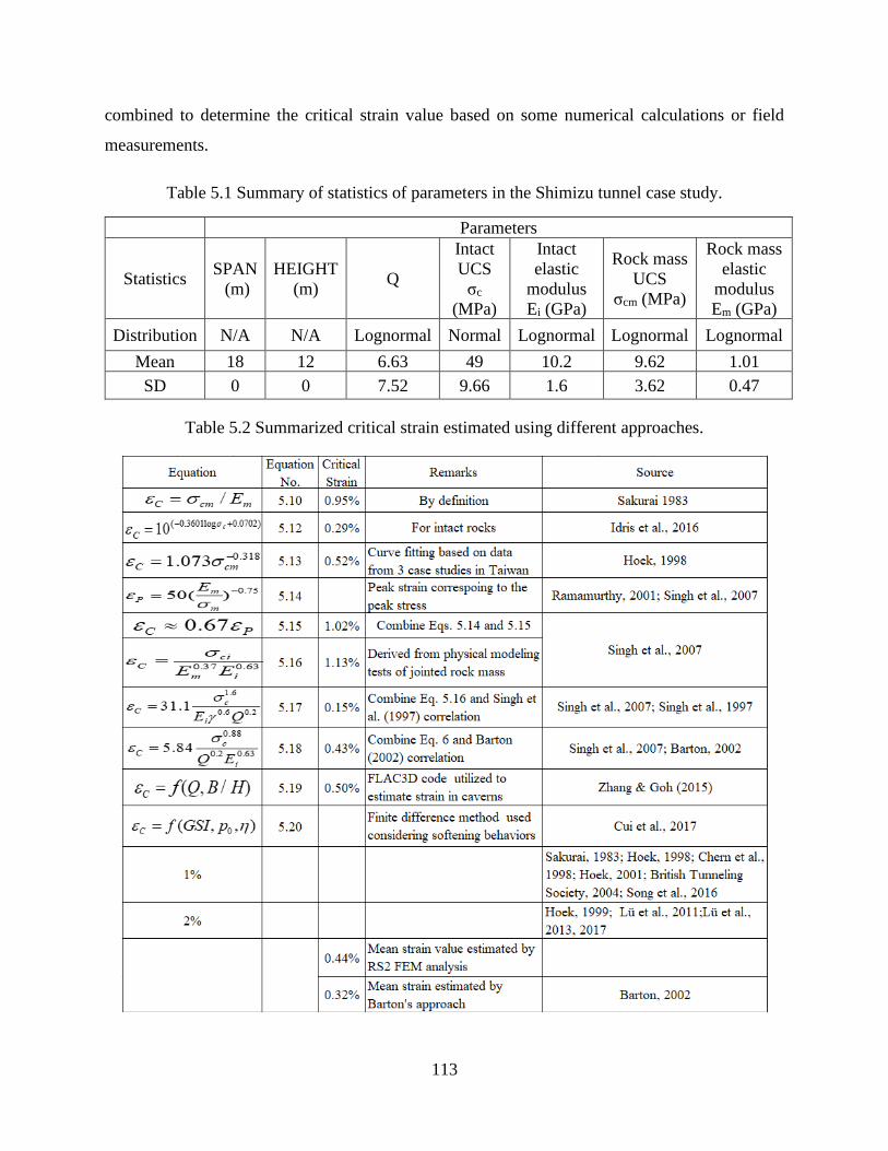
113
combined to determine the critical strain value based on some numerical calculations or field
measurements.
Table 5.1 Summary of statistics of parameters in the Shimizu tunnel case study.
Parameters
Statistics SPAN
(m)
HEIGHT
(m) Q
Intact
UCS
σc
(MPa)
Intact
elastic
modulus
Ei (GPa)
Rock mass
UCS
σcm (MPa)
Rock mass
elastic
modulus
Em (GPa)
Distribution N/A N/A Lognormal Normal Lognormal Lognormal Lognormal
Mean 18 12 6.63 49 10.2 9.62 1.01
SD 0 0 7.52 9.66 1.6 3.62 0.47
Table 5.2 Summarized critical strain estimated using different approaches.
114
5.4.2 Critical strain for intact rock and rock mass
The relationships between critical strain and uniaxial compressive strength (UCS) as well
as Young’s modulus of rocks and soils are summarized by (Sakurai, 2017), as seen in Figure 5.2.
Note that these relationships were established originally based on laboratory tests on rocks and
soils, however, Sakurai (1983) pointed out that the critical strain of in-situ rock mass is almost the
same order of magnitude as that of intact rocks based on in-situ tests (plate bearing tests and direct
shear tests) and back-calculations in rock masses. The critical strain for rock masses also falls
within the bounds shown in Figure 5.2 since the effects of joins are canceled out by taking the ratio
of the strength to the elastic modulus of rock mass (Sakurai, 1997). The hazard waring levels were
also proposed in the critical strain chart for preliminary evaluation of the stability of tunnels prior
to the start of tunnel excavation, which have three stages depending on the degree of stability. As
can be seen in Table 5.2 (A), the warning level III is the upper bound of the strain, above which
many different types of excavation problems are likely to occur; the warning level I is the lower
bound, below which tunnels are stable without excavation problems; and the warning level II in
between is the centerline between warning level I (lower bound) and warning level III (upper
bound). The upper bound and lower bound are also shown in Table 5.2 (B) in terms of the
relationship between critical strain and elastic modulus.
Based on the relationships shown in Figure 5.2, the hazard warning levels were estimated
using the strength and elastic moduli of intact rocks and rock mass in the Shimizu tunnel case, as
marked in Figure 5.2. The obtained hazard warning levels of critical strain are summarized in
Table 5.3. The critical strain values for intact rocks vary from about 0.1% to 0.8% based on the
intact UCS and elastic modulus according to Figure 5.2. In contrast, the critical strain values for
the rock mass are in the range of about 0.2% to about 1.5% based on the rock mass UCS and elastic
modulus values. Thus, it reveals that the critical strain values estimated for the rock mass are about
2 times that for intact rocks in this case study.
Sakurai (1997) stated that the critical strain of the rock mass is always greater (1 to 3 times
more) than that for intact rocks. Based on this, it is also suggested that the critical strain obtained
from intact rocks can be used as the permissible strain for rock mass since a certain amount of
safety allowance can be guaranteed. However, Daraei and Zare (2019) pointed out that the use of
critical strain derived from intact rocks is too conservative due to the following reasons: first, there
is a scale effect between rock mass and intact rocks and the critical strain for rock mass is about 1
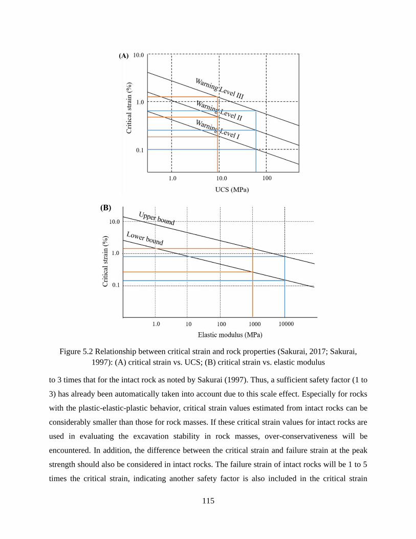
115
Figure 5.2 Relationship between critical strain and rock properties (Sakurai, 2017; Sakurai,
1997): (A) critical strain vs. UCS; (B) critical strain vs. elastic modulus
to 3 times that for the intact rock as noted by Sakurai (1997). Thus, a sufficient safety factor (1 to
3) has already been automatically taken into account due to this scale effect. Especially for rocks
with the plastic-elastic-plastic behavior, critical strain values estimated from intact rocks can be
considerably smaller than those for rock masses. If these critical strain values for intact rocks are
used in evaluating the excavation stability in rock masses, over-conservativeness will be
encountered. In addition, the difference between the critical strain and failure strain at the peak
strength should also be considered in intact rocks. The failure strain of intact rocks will be 1 to 5
times the critical strain, indicating another safety factor is also included in the critical strain
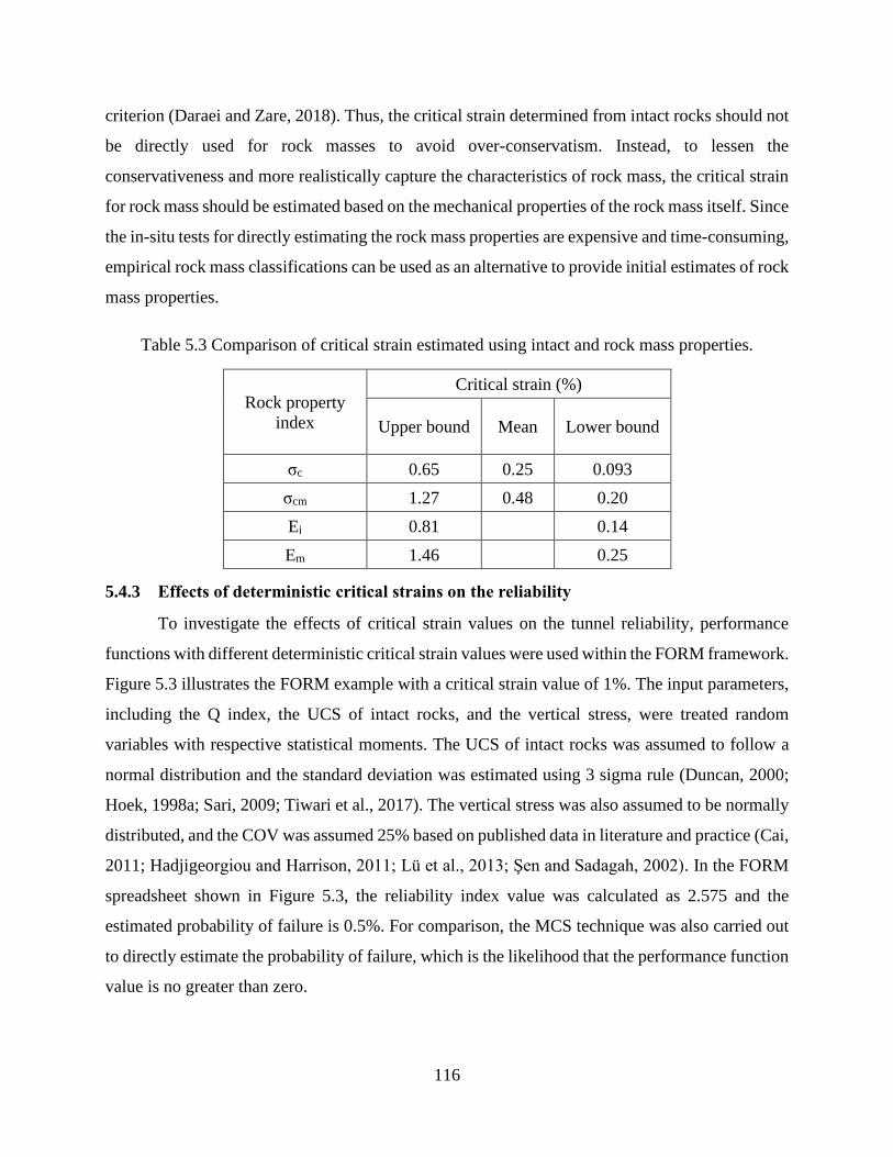
116
criterion (Daraei and Zare, 2018). Thus, the critical strain determined from intact rocks should not
be directly used for rock masses to avoid over-conservatism. Instead, to lessen the
conservativeness and more realistically capture the characteristics of rock mass, the critical strain
for rock mass should be estimated based on the mechanical properties of the rock mass itself. Since
the in-situ tests for directly estimating the rock mass properties are expensive and time-consuming,
empirical rock mass classifications can be used as an alternative to provide initial estimates of rock
mass properties.
Table 5.3 Comparison of critical strain estimated using intact and rock mass properties.
Rock property
index
Critical strain (%)
Upper bound Mean Lower bound
σc 0.65 0.25 0.093
σcm 1.27 0.48 0.20
Ei 0.81 0.14
Em 1.46 0.25
5.4.3 Effects of deterministic critical strains on the reliability
To investigate the effects of critical strain values on the tunnel reliability, performance
functions with different deterministic critical strain values were used within the FORM framework.
Figure 5.3 illustrates the FORM example with a critical strain value of 1%. The input parameters,
including the Q index, the UCS of intact rocks, and the vertical stress, were treated random
variables with respective statistical moments. The UCS of intact rocks was assumed to follow a
normal distribution and the standard deviation was estimated using 3 sigma rule (Duncan, 2000;
Hoek, 1998a; Sari, 2009; Tiwari et al., 2017). The vertical stress was also assumed to be normally
distributed, and the COV was assumed 25% based on published data in literature and practice (Cai,
2011; Hadjigeorgiou and Harrison, 2011; Lü et al., 2013; Şen and Sadagah, 2002). In the FORM
spreadsheet shown in Figure 5.3, the reliability index value was calculated as 2.575 and the
estimated probability of failure is 0.5%. For comparison, the MCS technique was also carried out
to directly estimate the probability of failure, which is the likelihood that the performance function
value is no greater than zero.
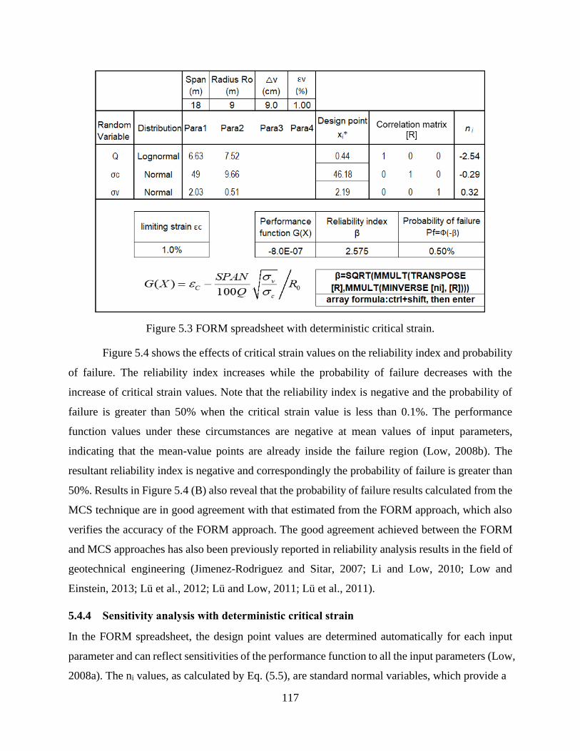
117
Figure 5.3 FORM spreadsheet with deterministic critical strain.
Figure 5.4 shows the effects of critical strain values on the reliability index and probability
of failure. The reliability index increases while the probability of failure decreases with the
increase of critical strain values. Note that the reliability index is negative and the probability of
failure is greater than 50% when the critical strain value is less than 0.1%. The performance
function values under these circumstances are negative at mean values of input parameters,
indicating that the mean-value points are already inside the failure region (Low, 2008b). The
resultant reliability index is negative and correspondingly the probability of failure is greater than
50%. Results in Figure 5.4 (B) also reveal that the probability of failure results calculated from the
MCS technique are in good agreement with that estimated from the FORM approach, which also
verifies the accuracy of the FORM approach. The good agreement achieved between the FORM
and MCS approaches has also been previously reported in reliability analysis results in the field of
geotechnical engineering (Jimenez-Rodriguez and Sitar, 2007; Li and Low, 2010; Low and
Einstein, 2013; Lü et al., 2012; Lü and Low, 2011; Lü et al., 2011).
5.4.4 Sensitivity analysis with deterministic critical strain
In the FORM spreadsheet, the design point values are determined automatically for each input
parameter and can reflect sensitivities of the performance function to all the input parameters (Low,
2008a). The ni values, as calculated by Eq. (5.5), are standard normal variables, which provide a

118
Figure 5.4 Effects of the critical strain on the reliability: (A) reliability index; (B) probability of
failure
measure of relative parametric sensitivity. The greater the ni value for an input parameter is, the
farther the design point is from the mean value point, and thus the more significant the input
parameter is. It is clearly seen in the ni column in Figure 5.3 that the ni value for the Q index is the
largest, followed by the vertical stress and the UCS. Using the MCS technique, the sensitivities of
input distributions can also be obtained with tornado graphs. Figure 5.5 illustrates the rank of
relative importance of input parameters in tornado graphs derived from the regression analysis in
the MCS process. The input parameter Q index is the most important, followed by the verticalstress
and the UCS, which is consistent with the sensitivity results derived from ni values in the FORM
spreadsheet.
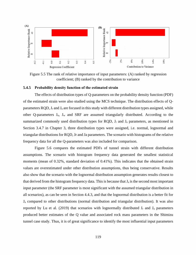
119
Figure 5.5 The rank of relative importance of input parameters: (A) ranked by regression
coefficient; (B) ranked by the contribution to variance
5.4.5 Probability density function of the estimated strain
The effects of distribution types of Q-parameters on the probability density function (PDF)
of the estimated strain were also studied using the MCS technique. The distribution effects of Q-
parameters RQD, Jr and Ja are focused in this study with different distribution types assigned, while
other Q-parameters Jn, Jw and SRF are assumed triangularly distributed. According to the
summarized commonly used distribution types for RQD, Jr and Ja parameters, as mentioned in
Section 3.4.7 in Chapter 3, three distribution types were assigned, i.e. normal, lognormal and
triangular distributions for RQD, Jr and Ja parameters. The scenario with histograms of the relative
frequency data for all the Q-parameters was also included for comparison.
Figure 5.6 compares the estimated PDFs of tunnel strain with different distribution
assumptions. The scenario with histogram frequency data generated the smallest statistical
moments (mean of 0.32%, standard deviation of 0.41%). This indicates that the obtained strain
values are overestimated under other distribution assumptions, thus being conservative. Results
also show that the scenario with the lognormal distribution assumption generates results closest to
that derived from the histogram frequency data. This is because that Ja is the second most important
input parameter (the SRF parameter is most significant with the assumed triangular distribution in
all scenarios), as can be seen in Section 4.4.3, and that the lognormal distribution is a better fit for
Ja compared to other distributions (normal distribution and triangular distribution). It was also
reported by Lu et al. (2019) that scenarios with lognormally distributed Jr and Ja parameters
produced better estimates of the Q value and associated rock mass parameters in the Shimizu
tunnel case study. Thus, it is of great significance to identify the most influential input parameters
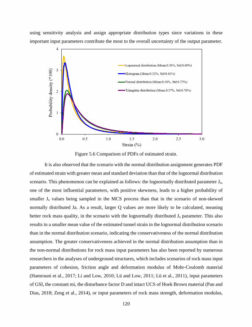
120
using sensitivity analysis and assign appropriate distribution types since variations in these
important input parameters contribute the most to the overall uncertainty of the output parameter.
Figure 5.6 Comparison of PDFs of estimated strain.
It is also observed that the scenario with the normal distribution assignment generates PDF
of estimated strain with greater mean and standard deviation than that of the lognormal distribution
scenario. This phenomenon can be explained as follows: the lognormally distributed parameter Ja,
one of the most influential parameters, with positive skewness, leads to a higher probability of
smaller Ja values being sampled in the MCS process than that in the scenario of non-skewed
normally distributed Ja. As a result, larger Q values are more likely to be calculated, meaning
better rock mass quality, in the scenario with the lognormally distributed Ja parameter. This also
results in a smaller mean value of the estimated tunnel strain in the lognormal distribution scenario
than in the normal distribution scenario, indicating the conservativeness of the normal distribution
assumption. The greater conservativeness achieved in the normal distribution assumption than in
the non-normal distributions for rock mass input parameters has also been reported by numerous
researchers in the analyses of underground structures, which includes scenarios of rock mass input
parameters of cohesion, friction angle and deformation modulus of Mohr-Coulomb material
(Hamrouni et al., 2017; Li and Low, 2010; Lü and Low, 2011; Lü et al., 2011), input parameters
of GSI, the constant mi, the disturbance factor D and intact UCS of Hoek Brown material (Pan and
Dias, 2018; Zeng et al., 2014), or input parameters of rock mass strength, deformation modulus,

121
Hoek-Brown criterion parameter m and dilation angle (Song et al., 2016). It is also found in Figure
5.6 that the scenario with triangular distribution assignment has the largest statistics of estimated
strain, generating the greatest differences compared to the results obtained from the histogram
scenario. This implies that the triangular distribution might not be suggested for use despite the
relative ease and simplicity in defining the distribution (min, most likely and max).
5.4.6 Effects of correlation between RQD and Jn on the reliability
The effects of the negative correlation between RQD and Jn on the reliability were also
studied. Figure 5.7 describes the variation of the reliability index and the probability of failure with
the changes of correlation coefficient between RQD and Jn. Results show that the lower safety
levels are achieved, represented by lower reliability index and higher probability of failure, with
stronger correlation between RQD and Jn. This indicates that the level of safety and reliability is
overestimated if the negative correlation is neglected. Recall that the greater mean of the Q value
is achieved with the stronger correlation between RQD and Jn, as mentioned in Section 3.4.6 in
Chapter 3 and Section 4.4.5 in Chapter 4, and this may lead to better rock mass quality as well as
higher reliability level. It should be noted, however, that the standard deviation and the COV which
are the measure of variation also become greater with stronger correlation between RQD and Jn.
As mentioned in Section 4.4.5 in Chapter 4, the standard deviation and COV are more sensitive to
the correlation between RQD and Jn compared to the mean values. Thus, it is indicated that the
dispersion in the derived distribution of the Q value may have greater effects on the overall level
of safety and reliability than the mean value.
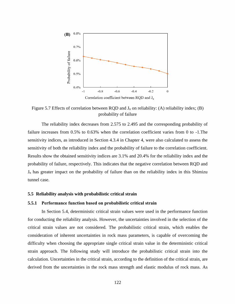
122
Figure 5.7 Effects of correlation between RQD and Jn on reliability: (A) reliability index; (B)
probability of failure
The reliability index decreases from 2.575 to 2.495 and the corresponding probability of
failure increases from 0.5% to 0.63% when the correlation coefficient varies from 0 to -1.The
sensitivity indices, as introduced in Section 4.3.4 in Chapter 4, were also calculated to assess the
sensitivity of both the reliability index and the probability of failure to the correlation coefficient.
Results show the obtained sensitivity indices are 3.1% and 20.4% for the reliability index and the
probability of failure, respectively. This indicates that the negative correlation between RQD and
Jn has greater impact on the probability of failure than on the reliability index in this Shimizu
tunnel case.
5.5 Reliability analysis with probabilistic critical strain
5.5.1 Performance function based on probabilistic critical strain
In Section 5.4, deterministic critical strain values were used in the performance function
for conducting the reliability analysis. However, the uncertainties involved in the selection of the
critical strain values are not considered. The probabilistic critical strain, which enables the
consideration of inherent uncertainties in rock mass parameters, is capable of overcoming the
difficulty when choosing the appropriate single critical strain value in the deterministic critical
strain approach. The following study will introduce the probabilistic critical strain into the
calculation. Uncertainties in the critical strain, according to the definition of the critical strain, are
derived from the uncertainties in the rock mass strength and elastic modulus of rock mass. As
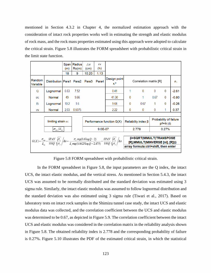
123
mentioned in Section 4.3.2 in Chapter 4, the normalized estimation approach with the
consideration of intact rock properties works well in estimating the strength and elastic modulus
of rock mass, and the rock mass properties estimated using this approach were adopted to calculate
the critical strain. Figure 5.8 illustrates the FORM spreadsheet with probabilistic critical strain in
the limit state function.
Figure 5.8 FORM spreadsheet with probabilistic critical strain.
In the FORM spreadsheet in Figure 5.8, the input parameters are the Q index, the intact
UCS, the intact elastic modulus, and the vertical stress. As mentioned in Section 5.4.3, the intact
UCS was assumed to be normally distributed and the standard deviation was estimated using 3
sigma rule. Similarly, the intact elastic modulus was assumed to follow lognormal distribution and
the standard deviation was also estimated using 3 sigma rule (Tiwari et al., 2017). Based on
laboratory tests on intact rock samples in the Shimizu tunnel case study, the intact UCS and elastic
modulus data was collected, and the correlation coefficient between the UCS and elastic modulus
was determined to be 0.67, as depicted in Figure 5.9. The correlation coefficient between the intact
UCS and elastic modulus was considered in the correlation matrix in the reliability analysis shown
in Figure 5.8. The obtained reliability index is 2.778 and the corresponding probability of failure
is 0.27%. Figure 5.10 illustrates the PDF of the estimated critical strain, in which the statistical
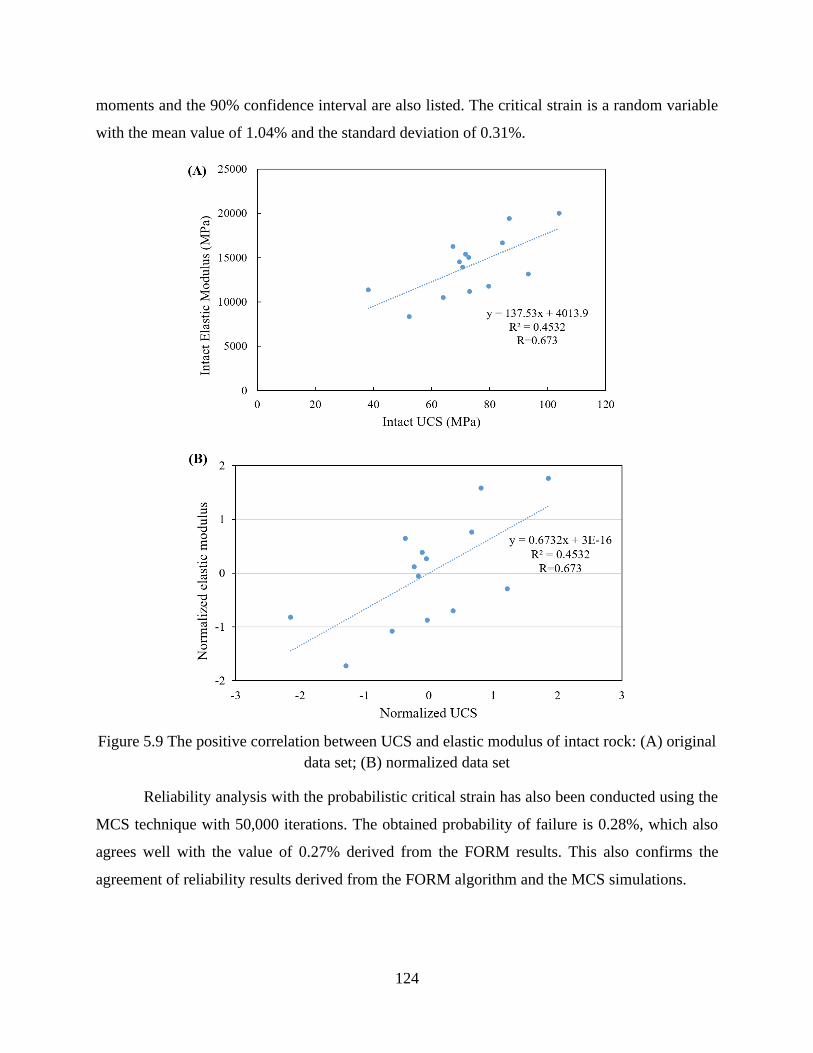
124
moments and the 90% confidence interval are also listed. The critical strain is a random variable
with the mean value of 1.04% and the standard deviation of 0.31%.
Figure 5.9 The positive correlation between UCS and elastic modulus of intact rock: (A) original
data set; (B) normalized data set
Reliability analysis with the probabilistic critical strain has also been conducted using the
MCS technique with 50,000 iterations. The obtained probability of failure is 0.28%, which also
agrees well with the value of 0.27% derived from the FORM results. This also confirms the
agreement of reliability results derived from the FORM algorithm and the MCS simulations.
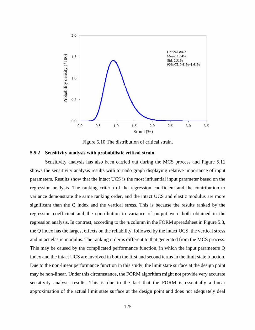
125
Figure 5.10 The distribution of critical strain.
5.5.2 Sensitivity analysis with probabilistic critical strain
Sensitivity analysis has also been carried out during the MCS process and Figure 5.11
shows the sensitivity analysis results with tornado graph displaying relative importance of input
parameters. Results show that the intact UCS is the most influential input parameter based on the
regression analysis. The ranking criteria of the regression coefficient and the contribution to
variance demonstrate the same ranking order, and the intact UCS and elastic modulus are more
significant than the Q index and the vertical stress. This is because the results ranked by the
regression coefficient and the contribution to variance of output were both obtained in the
regression analysis. In contrast, according to the ni column in the FORM spreadsheet in Figure 5.8,
the Q index has the largest effects on the reliability, followed by the intact UCS, the vertical stress
and intact elastic modulus. The ranking order is different to that generated from the MCS process.
This may be caused by the complicated performance function, in which the input parameters Q
index and the intact UCS are involved in both the first and second terms in the limit state function.
Due to the non-linear performance function in this study, the limit state surface at the design point
may be non-linear. Under this circumstance, the FORM algorithm might not provide very accurate
sensitivity analysis results. This is due to the fact that the FORM is essentially a linear
approximation of the actual limit state surface at the design point and does not adequately deal
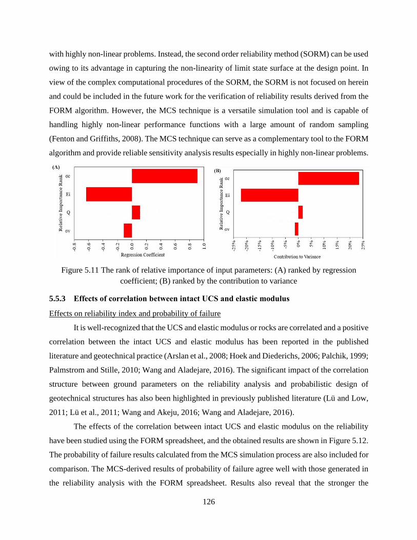
126
with highly non-linear problems. Instead, the second order reliability method (SORM) can be used
owing to its advantage in capturing the non-linearity of limit state surface at the design point. In
view of the complex computational procedures of the SORM, the SORM is not focused on herein
and could be included in the future work for the verification of reliability results derived from the
FORM algorithm. However, the MCS technique is a versatile simulation tool and is capable of
handling highly non-linear performance functions with a large amount of random sampling
(Fenton and Griffiths, 2008). The MCS technique can serve as a complementary tool to the FORM
algorithm and provide reliable sensitivity analysis results especially in highly non-linear problems.
Figure 5.11 The rank of relative importance of input parameters: (A) ranked by regression
coefficient; (B) ranked by the contribution to variance
5.5.3 Effects of correlation between intact UCS and elastic modulus
Effects on reliability index and probability of failure
It is well-recognized that the UCS and elastic modulus or rocks are correlated and a positive
correlation between the intact UCS and elastic modulus has been reported in the published
literature and geotechnical practice (Arslan et al., 2008; Hoek and Diederichs, 2006; Palchik, 1999;
Palmstrom and Stille, 2010; Wang and Aladejare, 2016). The significant impact of the correlation
structure between ground parameters on the reliability analysis and probabilistic design of
geotechnical structures has also been highlighted in previously published literature (Lü and Low,
2011; Lü et al., 2011; Wang and Akeju, 2016; Wang and Aladejare, 2016).
The effects of the correlation between intact UCS and elastic modulus on the reliability
have been studied using the FORM spreadsheet, and the obtained results are shown in Figure 5.12.
The probability of failure results calculated from the MCS simulation process are also included for
comparison. The MCS-derived results of probability of failure agree well with those generated in
the reliability analysis with the FORM spreadsheet. Results also reveal that the stronger the
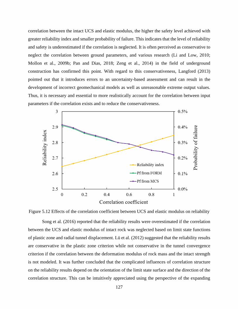
127
correlation between the intact UCS and elastic modulus, the higher the safety level achieved with
greater reliability index and smaller probability of failure. This indicates that the level of reliability
and safety is underestimated if the correlation is neglected. It is often perceived as conservative to
neglect the correlation between ground parameters, and various research (Li and Low, 2010;
Mollon et al., 2009b; Pan and Dias, 2018; Zeng et al., 2014) in the field of underground
construction has confirmed this point. With regard to this conservativeness, Langford (2013)
pointed out that it introduces errors to an uncertainty-based assessment and can result in the
development of incorrect geomechanical models as well as unreasonable extreme output values.
Thus, it is necessary and essential to more realistically account for the correlation between input
parameters if the correlation exists and to reduce the conservativeness.
Figure 5.12 Effects of the correlation coefficient between UCS and elastic modulus on reliability
Song et al. (2016) reported that the reliability results were overestimated if the correlation
between the UCS and elastic modulus of intact rock was neglected based on limit state functions
of plastic zone and radial tunnel displacement. Lü et al. (2012) suggested that the reliability results
are conservative in the plastic zone criterion while not conservative in the tunnel convergence
criterion if the correlation between the deformation modulus of rock mass and the intact strength
is not modeled. It was further concluded that the complicated influences of correlation structure
on the reliability results depend on the orientation of the limit state surface and the direction of the
correlation structure. This can be intuitively appreciated using the perspective of the expanding
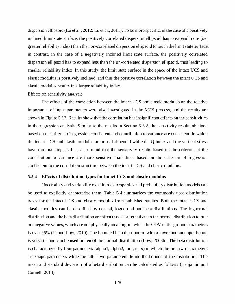
128
dispersion ellipsoid (Lü et al., 2012; Lü et al., 2011). To be more specific, in the case of a positively
inclined limit state surface, the positively correlated dispersion ellipsoid has to expand more (i.e.
greater reliability index) than the non-correlated dispersion ellipsoid to touch the limit state surface;
in contrast, in the case of a negatively inclined limit state surface, the positively correlated
dispersion ellipsoid has to expand less than the un-correlated dispersion ellipsoid, thus leading to
smaller reliability index. In this study, the limit state surface in the space of the intact UCS and
elastic modulus is positively inclined, and thus the positive correlation between the intact UCS and
elastic modulus results in a larger reliability index.
Effects on sensitivity analysis
The effects of the correlation between the intact UCS and elastic modulus on the relative
importance of input parameters were also investigated in the MCS process, and the results are
shown in Figure 5.13. Results show that the correlation has insignificant effects on the sensitivities
in the regression analysis. Similar to the results in Section 5.5.2, the sensitivity results obtained
based on the criteria of regression coefficient and contribution to variance are consistent, in which
the intact UCS and elastic modulus are most influential while the Q index and the vertical stress
have minimal impact. It is also found that the sensitivity results based on the criterion of the
contribution to variance are more sensitive than those based on the criterion of regression
coefficient to the correlation structure between the intact UCS and elastic modulus.
5.5.4 Effects of distribution types for intact UCS and elastic modulus
Uncertainty and variability exist in rock properties and probability distribution models can
be used to explicitly characterize them. Table 5.4 summarizes the commonly used distribution
types for the intact UCS and elastic modulus from published studies. Both the intact UCS and
elastic modulus can be described by normal, lognormal and beta distributions. The lognormal
distribution and the beta distribution are often used as alternatives to the normal distribution to rule
out negative values, which are not physically meaningful, when the COV of the ground parameters
is over 25% (Li and Low, 2010). The bounded beta distribution with a lower and an upper bound
is versatile and can be used in lieu of the normal distribution (Low, 2008b). The beta distribution
is characterized by four parameters (alpha1, alpha2, min, max) in which the first two parameters
are shape parameters while the latter two parameters define the bounds of the distribution. The
mean and standard deviation of a beta distribution can be calculated as follows (Benjamin and
Cornell, 2014):
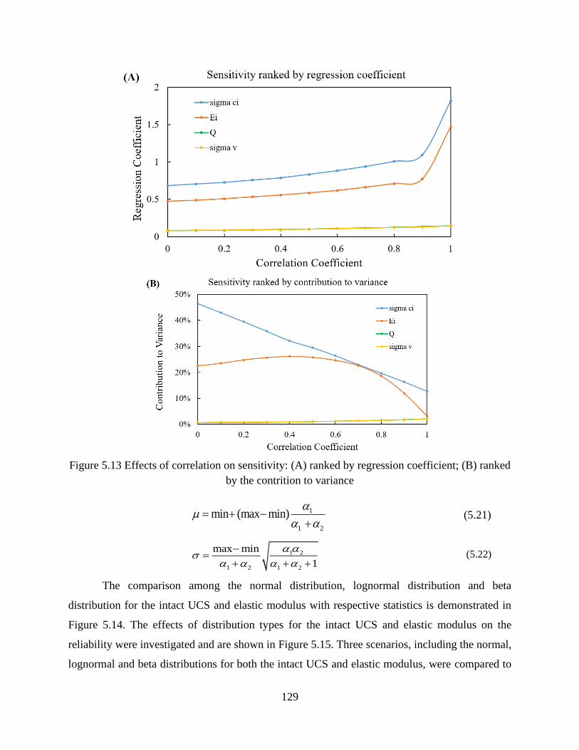
129
Figure 5.13 Effects of correlation on sensitivity: (A) ranked by regression coefficient; (B) ranked
by the contrition to variance
1
1 2
min (max min)
= + −+
(5.21)
1 2
1 2 1 2
max min
1
−=
+ + + (5.22)
The comparison among the normal distribution, lognormal distribution and beta
distribution for the intact UCS and elastic modulus with respective statistics is demonstrated in
Figure 5.14. The effects of distribution types for the intact UCS and elastic modulus on the
reliability were investigated and are shown in Figure 5.15. Three scenarios, including the normal,
lognormal and beta distributions for both the intact UCS and elastic modulus, were compared to
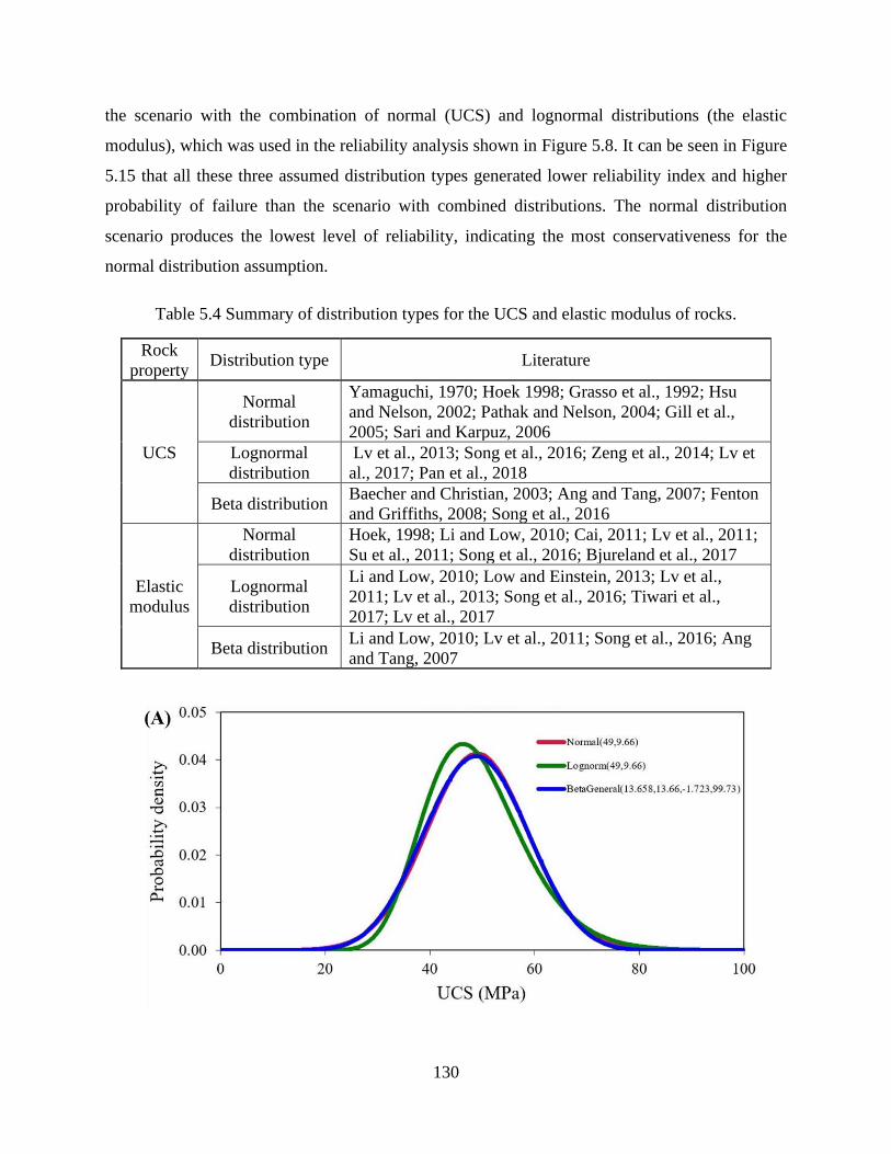
130
the scenario with the combination of normal (UCS) and lognormal distributions (the elastic
modulus), which was used in the reliability analysis shown in Figure 5.8. It can be seen in Figure
5.15 that all these three assumed distribution types generated lower reliability index and higher
probability of failure than the scenario with combined distributions. The normal distribution
scenario produces the lowest level of reliability, indicating the most conservativeness for the
normal distribution assumption.
Table 5.4 Summary of distribution types for the UCS and elastic modulus of rocks.
Rock
property Distribution type Literature
UCS
Normal
distribution
Yamaguchi, 1970; Hoek 1998; Grasso et al., 1992; Hsu
and Nelson, 2002; Pathak and Nelson, 2004; Gill et al.,
2005; Sari and Karpuz, 2006
Lognormal
distribution
Lv et al., 2013; Song et al., 2016; Zeng et al., 2014; Lv et
al., 2017; Pan et al., 2018
Beta distribution Baecher and Christian, 2003; Ang and Tang, 2007; Fenton
and Griffiths, 2008; Song et al., 2016
Elastic
modulus
Normal
distribution
Hoek, 1998; Li and Low, 2010; Cai, 2011; Lv et al., 2011;
Su et al., 2011; Song et al., 2016; Bjureland et al., 2017
Lognormal
distribution
Li and Low, 2010; Low and Einstein, 2013; Lv et al.,
2011; Lv et al., 2013; Song et al., 2016; Tiwari et al.,
2017; Lv et al., 2017
Beta distribution Li and Low, 2010; Lv et al., 2011; Song et al., 2016; Ang
and Tang, 2007
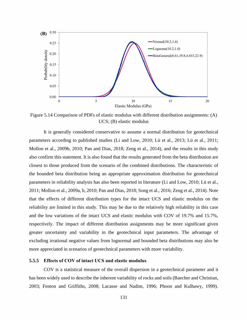
131
Figure 5.14 Comparison of PDFs of elastic modulus with different distribution assignments: (A)
UCS; (B) elastic modulus
It is generally considered conservative to assume a normal distribution for geotechnical
parameters according to published studies (Li and Low, 2010; Lü et al., 2013; Lü et al., 2011;
Mollon et al., 2009b, 2010; Pan and Dias, 2018; Zeng et al., 2014), and the results in this study
also confirm this statement. It is also found that the results generated from the beta distribution are
closest to those produced from the scenario of the combined distributions. The characteristic of
the bounded beta distribution being an appropriate approximation distribution for geotechnical
parameters in reliability analysis has also been reported in literature (Li and Low, 2010; Lü et al.,
2011; Mollon et al., 2009a, b, 2010; Pan and Dias, 2018; Song et al., 2016; Zeng et al., 2014). Note
that the effects of different distribution types for the intact UCS and elastic modulus on the
reliability are limited in this study. This may be due to the relatively high reliability in this case
and the low variations of the intact UCS and elastic modulus with COV of 19.7% and 15.7%,
respectively. The impact of different distribution assignments may be more significant given
greater uncertainty and variability in the geotechnical input parameters. The advantage of
excluding irrational negative values from lognormal and bounded beta distributions may also be
more appreciated in scenarios of geotechnical parameters with more variability.
5.5.5 Effects of COV of intact UCS and elastic modulus
COV is a statistical measure of the overall dispersion in a geotechnical parameter and it
has been widely used to describe the inherent variability of rocks and soils (Baecher and Christian,
2003; Fenton and Griffiths, 2008; Lacasse and Nadim, 1996; Phoon and Kulhawy, 1999).
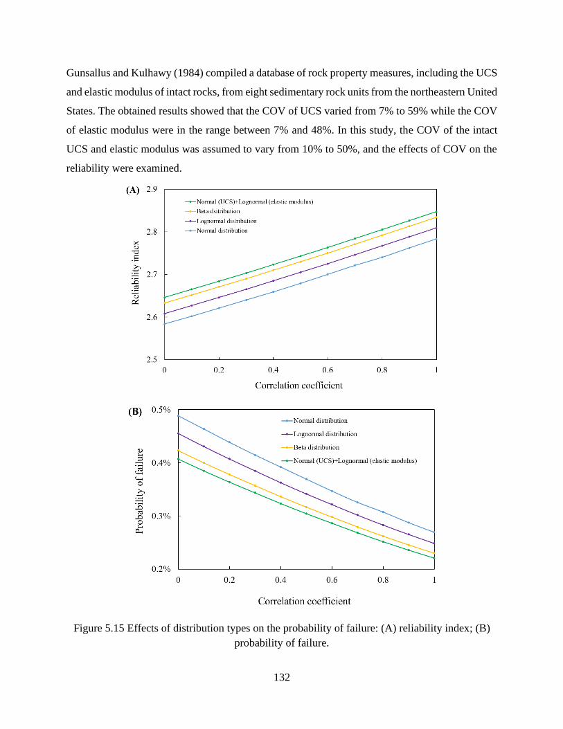
132
Gunsallus and Kulhawy (1984) compiled a database of rock property measures, including the UCS
and elastic modulus of intact rocks, from eight sedimentary rock units from the northeastern United
States. The obtained results showed that the COV of UCS varied from 7% to 59% while the COV
of elastic modulus were in the range between 7% and 48%. In this study, the COV of the intact
UCS and elastic modulus was assumed to vary from 10% to 50%, and the effects of COV on the
reliability were examined.
Figure 5.15 Effects of distribution types on the probability of failure: (A) reliability index; (B)
probability of failure.
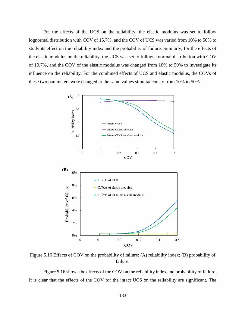
133
For the effects of the UCS on the reliability, the elastic modulus was set to follow
lognormal distribution with COV of 15.7%, and the COV of UCS was varied from 10% to 50% to
study its effect on the reliability index and the probability of failure. Similarly, for the effects of
the elastic modulus on the reliability, the UCS was set to follow a normal distribution with COV
of 19.7%, and the COV of the elastic modulus was changed from 10% to 50% to investigate its
influence on the reliability. For the combined effects of UCS and elastic modulus, the COVs of
these two parameters were changed to the same values simultaneously from 10% to 50%.
Figure 5.16 Effects of COV on the probability of failure: (A) reliability index; (B) probability of
failure.
Figure 5.16 shows the effects of the COV on the reliability index and probability of failure.
It is clear that the effects of the COV for the intact UCS on the reliability are significant. The
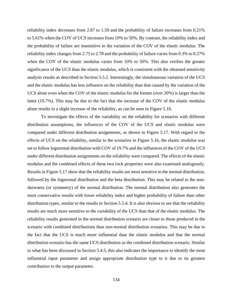
134
reliability index decreases from 2.87 to 1.59 and the probability of failure increases from 0.21%
to 5.61% when the COV of UCS increases from 10% to 50%. By contrast, the reliability index and
the probability of failure are insensitive to the variation of the COV of the elastic modulus. The
reliability index changes from 2.75 to 2.78 and the probability of failure varies from 0.3% to 0.27%
when the COV of the elastic modulus varies from 10% to 50%. This also verifies the greater
significance of the UCS than the elastic modulus, which is consistent with the obtained sensitivity
analysis results as described in Section 5.5.2. Interestingly, the simultaneous variation of the UCS
and the elastic modulus has less influence on the reliability than that caused by the variation of the
UCS alone even when the COV of the elastic modulus for the former (over 20%) is larger than the
latter (19.7%). This may be due to the fact that the increase of the COV of the elastic modulus
alone results in a slight increase of the reliability, as can be seen in Figure 5.16.
To investigate the effects of the variability on the reliability for scenarios with different
distribution assumptions, the influences of the COV of the UCS and elastic modulus were
compared under different distribution assignments, as shown in Figure 5.17. With regard to the
effects of UCS on the reliability, similar to the scenarios in Figure 5.16, the elastic modulus was
set to follow lognormal distribution with COV of 19.7% and the influences of the COV of the UCS
under different distribution assignments on the reliability were compared. The effects of the elastic
modulus and the combined effects of these two rock properties were also examined analogously.
Results in Figure 5.17 show that the reliability results are most sensitive to the normal distribution,
followed by the lognormal distribution and the beta distribution. This may be related to the non-
skewness (or symmetry) of the normal distribution. The normal distribution also generates the
most conservative results with lower reliability index and higher probability of failure than other
distribution types, similar to the results in Section 5.5.4. It is also obvious to see that the reliability
results are much more sensitive to the variability of the UCS than that of the elastic modulus. The
reliability results generated in the normal distribution scenario are closer to those produced in the
scenario with combined distributions than non-normal distribution scenarios. This may be due to
the fact that the UCS is much more influential than the elastic modulus and that the normal
distribution scenario has the same UCS distribution as the combined distribution scenario. Similar
to what has been discussed in Section 5.4.5, this also indicates the importance to identify the most
influential input parameter and assign appropriate distribution type to it due to its greatest
contribution to the output parameter.

135
Figure 5.17 The effects of distribution types on the influences of COV on the probability of
failure.
5.5.6 Reliability evaluation on the excavation stability
Excavation stability evaluation using different approaches
Recall that the obtained reliability index is 2.778 and the probability of failure is 0.27%
with the probabilistic critical strain in the performance function, as shown in Figure 5.8. The target
reliability indices and corresponding probability of failure are summarized by USACE (1997) for
general structures in the geotechnical engineering field, as shown in Table 5.5. The probability of
failure value for the excavated Shimizu tunnel is 0.27%. The expected performance level is worse
than “above average” and better than “below average”.
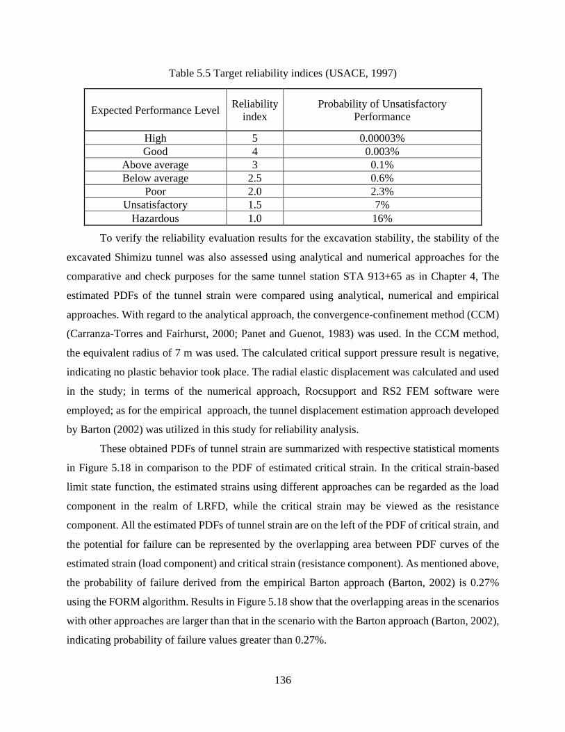
136
Table 5.5 Target reliability indices (USACE, 1997)
Expected Performance Level Reliability
index
Probability of Unsatisfactory
Performance
High 5 0.00003%
Good 4 0.003%
Above average 3 0.1%
Below average 2.5 0.6%
Poor 2.0 2.3%
Unsatisfactory 1.5 7%
Hazardous 1.0 16%
To verify the reliability evaluation results for the excavation stability, the stability of the
excavated Shimizu tunnel was also assessed using analytical and numerical approaches for the
comparative and check purposes for the same tunnel station STA 913+65 as in Chapter 4, The
estimated PDFs of the tunnel strain were compared using analytical, numerical and empirical
approaches. With regard to the analytical approach, the convergence-confinement method (CCM)
(Carranza-Torres and Fairhurst, 2000; Panet and Guenot, 1983) was used. In the CCM method,
the equivalent radius of 7 m was used. The calculated critical support pressure result is negative,
indicating no plastic behavior took place. The radial elastic displacement was calculated and used
in the study; in terms of the numerical approach, Rocsupport and RS2 FEM software were
employed; as for the empirical approach, the tunnel displacement estimation approach developed
by Barton (2002) was utilized in this study for reliability analysis.
These obtained PDFs of tunnel strain are summarized with respective statistical moments
in Figure 5.18 in comparison to the PDF of estimated critical strain. In the critical strain-based
limit state function, the estimated strains using different approaches can be regarded as the load
component in the realm of LRFD, while the critical strain may be viewed as the resistance
component. All the estimated PDFs of tunnel strain are on the left of the PDF of critical strain, and
the potential for failure can be represented by the overlapping area between PDF curves of the
estimated strain (load component) and critical strain (resistance component). As mentioned above,
the probability of failure derived from the empirical Barton approach (Barton, 2002) is 0.27%
using the FORM algorithm. Results in Figure 5.18 show that the overlapping areas in the scenarios
with other approaches are larger than that in the scenario with the Barton approach (Barton, 2002),
indicating probability of failure values greater than 0.27%.
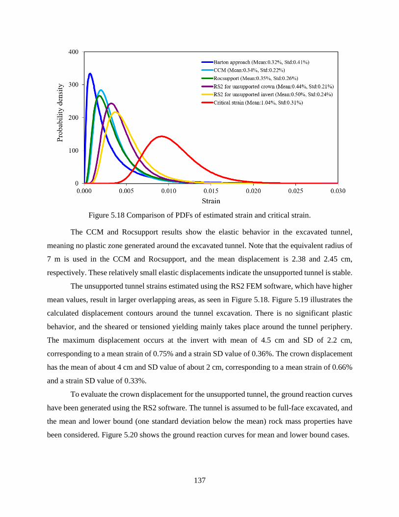
137
Figure 5.18 Comparison of PDFs of estimated strain and critical strain.
The CCM and Rocsupport results show the elastic behavior in the excavated tunnel,
meaning no plastic zone generated around the excavated tunnel. Note that the equivalent radius of
7 m is used in the CCM and Rocsupport, and the mean displacement is 2.38 and 2.45 cm,
respectively. These relatively small elastic displacements indicate the unsupported tunnel is stable.
The unsupported tunnel strains estimated using the RS2 FEM software, which have higher
mean values, result in larger overlapping areas, as seen in Figure 5.18. Figure 5.19 illustrates the
calculated displacement contours around the tunnel excavation. There is no significant plastic
behavior, and the sheared or tensioned yielding mainly takes place around the tunnel periphery.
The maximum displacement occurs at the invert with mean of 4.5 cm and SD of 2.2 cm,
corresponding to a mean strain of 0.75% and a strain SD value of 0.36%. The crown displacement
has the mean of about 4 cm and SD value of about 2 cm, corresponding to a mean strain of 0.66%
and a strain SD value of 0.33%.
To evaluate the crown displacement for the unsupported tunnel, the ground reaction curves
have been generated using the RS2 software. The tunnel is assumed to be full-face excavated, and
the mean and lower bound (one standard deviation below the mean) rock mass properties have
been considered. Figure 5.20 shows the ground reaction curves for mean and lower bound cases.
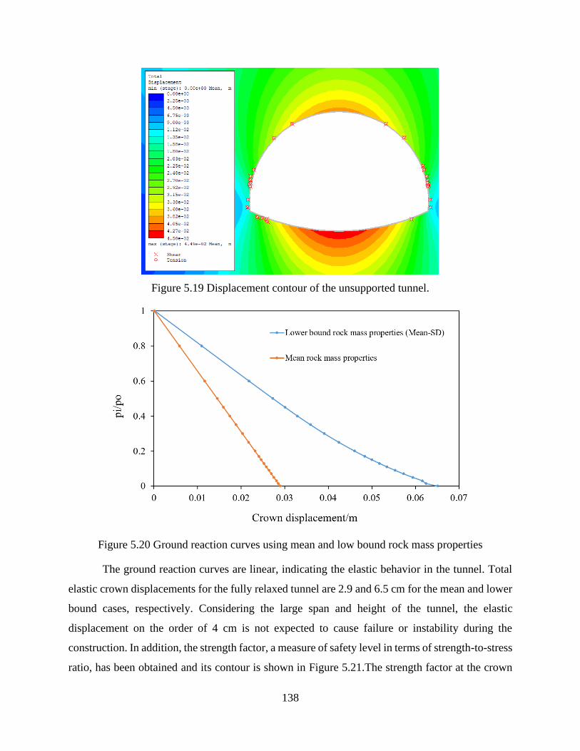
138
Figure 5.19 Displacement contour of the unsupported tunnel.
Figure 5.20 Ground reaction curves using mean and low bound rock mass properties
The ground reaction curves are linear, indicating the elastic behavior in the tunnel. Total
elastic crown displacements for the fully relaxed tunnel are 2.9 and 6.5 cm for the mean and lower
bound cases, respectively. Considering the large span and height of the tunnel, the elastic
displacement on the order of 4 cm is not expected to cause failure or instability during the
construction. In addition, the strength factor, a measure of safety level in terms of strength-to-stress
ratio, has been obtained and its contour is shown in Figure 5.21.The strength factor at the crown
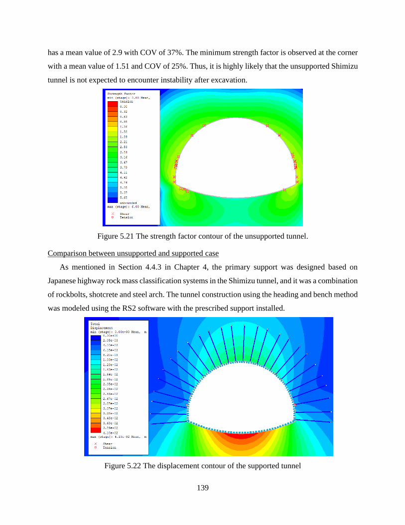
139
has a mean value of 2.9 with COV of 37%. The minimum strength factor is observed at the corner
with a mean value of 1.51 and COV of 25%. Thus, it is highly likely that the unsupported Shimizu
tunnel is not expected to encounter instability after excavation.
Figure 5.21 The strength factor contour of the unsupported tunnel.
Comparison between unsupported and supported case
As mentioned in Section 4.4.3 in Chapter 4, the primary support was designed based on
Japanese highway rock mass classification systems in the Shimizu tunnel, and it was a combination
of rockbolts, shotcrete and steel arch. The tunnel construction using the heading and bench method
was modeled using the RS2 software with the prescribed support installed.
Figure 5.22 The displacement contour of the supported tunnel
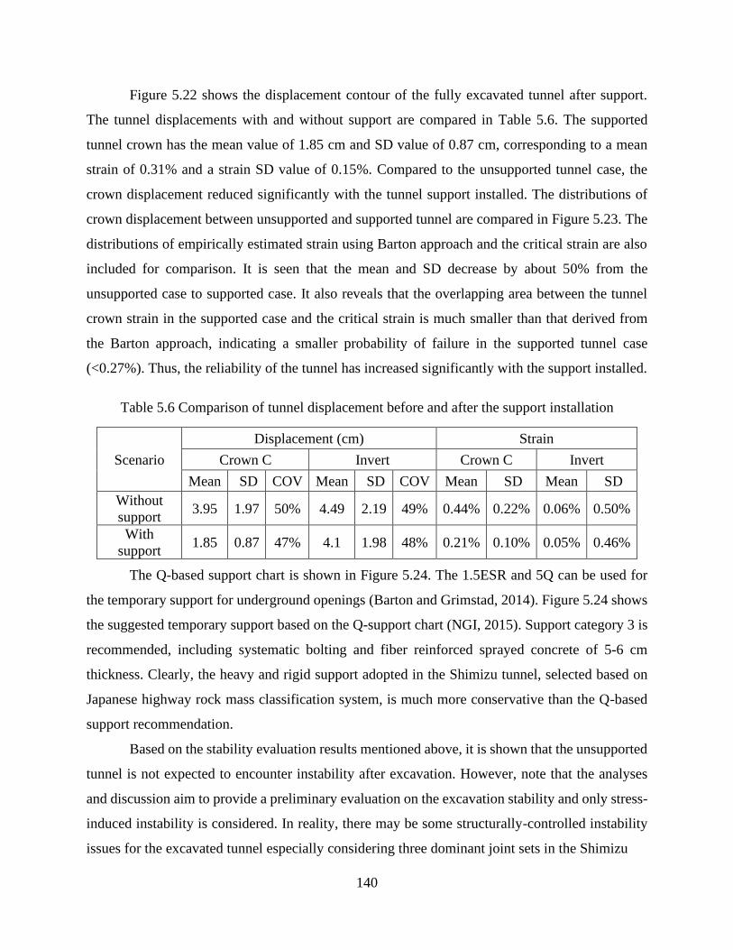
140
Figure 5.22 shows the displacement contour of the fully excavated tunnel after support.
The tunnel displacements with and without support are compared in Table 5.6. The supported
tunnel crown has the mean value of 1.85 cm and SD value of 0.87 cm, corresponding to a mean
strain of 0.31% and a strain SD value of 0.15%. Compared to the unsupported tunnel case, the
crown displacement reduced significantly with the tunnel support installed. The distributions of
crown displacement between unsupported and supported tunnel are compared in Figure 5.23. The
distributions of empirically estimated strain using Barton approach and the critical strain are also
included for comparison. It is seen that the mean and SD decrease by about 50% from the
unsupported case to supported case. It also reveals that the overlapping area between the tunnel
crown strain in the supported case and the critical strain is much smaller than that derived from
the Barton approach, indicating a smaller probability of failure in the supported tunnel case
(<0.27%). Thus, the reliability of the tunnel has increased significantly with the support installed.
Table 5.6 Comparison of tunnel displacement before and after the support installation
Scenario
Displacement (cm) Strain
Crown C Invert Crown C Invert
Mean SD COV Mean SD COV Mean SD Mean SD
Without
support 3.95 1.97 50% 4.49 2.19 49% 0.44% 0.22% 0.06% 0.50%
With
support 1.85 0.87 47% 4.1 1.98 48% 0.21% 0.10% 0.05% 0.46%
The Q-based support chart is shown in Figure 5.24. The 1.5ESR and 5Q can be used for
the temporary support for underground openings (Barton and Grimstad, 2014). Figure 5.24 shows
the suggested temporary support based on the Q-support chart (NGI, 2015). Support category 3 is
recommended, including systematic bolting and fiber reinforced sprayed concrete of 5-6 cm
thickness. Clearly, the heavy and rigid support adopted in the Shimizu tunnel, selected based on
Japanese highway rock mass classification system, is much more conservative than the Q-based
support recommendation.
Based on the stability evaluation results mentioned above, it is shown that the unsupported
tunnel is not expected to encounter instability after excavation. However, note that the analyses
and discussion aim to provide a preliminary evaluation on the excavation stability and only stress-
induced instability is considered. In reality, there may be some structurally-controlled instability
issues for the excavated tunnel especially considering three dominant joint sets in the Shimizu
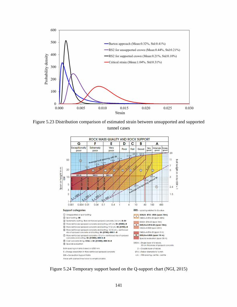
141
Figure 5.23 Distribution comparison of estimated strain between unsupported and supported
tunnel cases
Figure 5.24 Temporary support based on the Q-support chart (NGI, 2015)
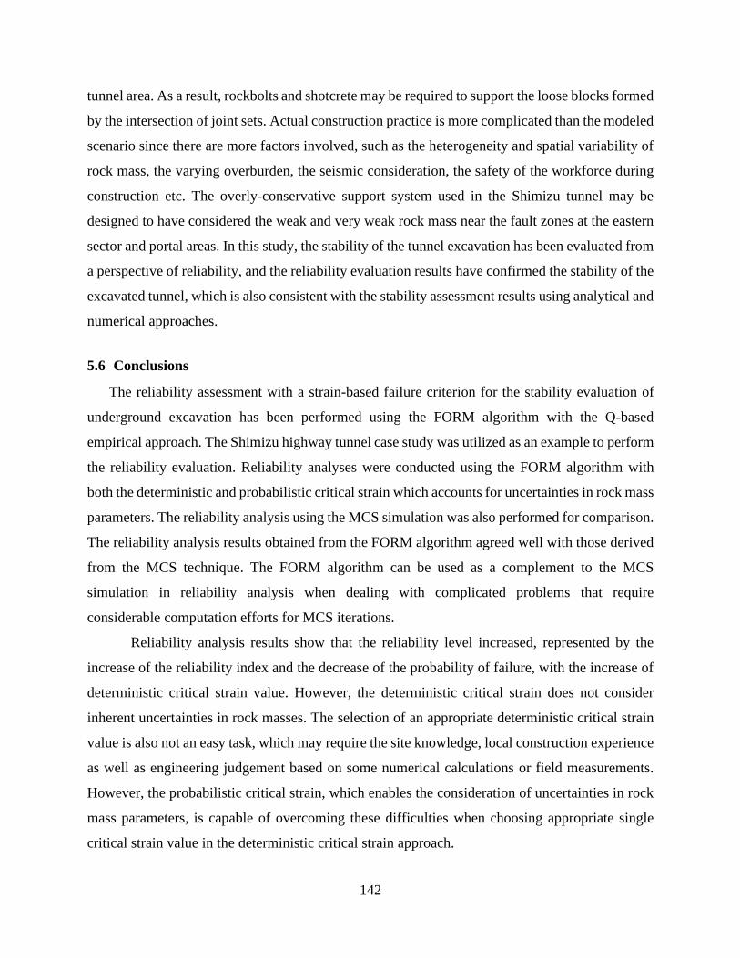
142
tunnel area. As a result, rockbolts and shotcrete may be required to support the loose blocks formed
by the intersection of joint sets. Actual construction practice is more complicated than the modeled
scenario since there are more factors involved, such as the heterogeneity and spatial variability of
rock mass, the varying overburden, the seismic consideration, the safety of the workforce during
construction etc. The overly-conservative support system used in the Shimizu tunnel may be
designed to have considered the weak and very weak rock mass near the fault zones at the eastern
sector and portal areas. In this study, the stability of the tunnel excavation has been evaluated from
a perspective of reliability, and the reliability evaluation results have confirmed the stability of the
excavated tunnel, which is also consistent with the stability assessment results using analytical and
numerical approaches.
5.6 Conclusions
The reliability assessment with a strain-based failure criterion for the stability evaluation of
underground excavation has been performed using the FORM algorithm with the Q-based
empirical approach. The Shimizu highway tunnel case study was utilized as an example to perform
the reliability evaluation. Reliability analyses were conducted using the FORM algorithm with
both the deterministic and probabilistic critical strain which accounts for uncertainties in rock mass
parameters. The reliability analysis using the MCS simulation was also performed for comparison.
The reliability analysis results obtained from the FORM algorithm agreed well with those derived
from the MCS technique. The FORM algorithm can be used as a complement to the MCS
simulation in reliability analysis when dealing with complicated problems that require
considerable computation efforts for MCS iterations.
Reliability analysis results show that the reliability level increased, represented by the
increase of the reliability index and the decrease of the probability of failure, with the increase of
deterministic critical strain value. However, the deterministic critical strain does not consider
inherent uncertainties in rock masses. The selection of an appropriate deterministic critical strain
value is also not an easy task, which may require the site knowledge, local construction experience
as well as engineering judgement based on some numerical calculations or field measurements.
However, the probabilistic critical strain, which enables the consideration of uncertainties in rock
mass parameters, is capable of overcoming these difficulties when choosing appropriate single
critical strain value in the deterministic critical strain approach.
143
The effects of correlation in input parameters on the reliability were investigated. Results
show that the negative correlation between RQD and Jn had limited influence on the reliability.
The positive correlation between the intact UCS and elastic modulus was also examined, and it
was found that the reliability results would be conservative if the positive correlation between the
intact UCS and elastic modulus is overlooked. In addition, the effects of distribution types for the
intact UCS and elastic modulus were also studied. The normal distribution assignment generated
the most conservative reliability results. Thus, the assumption of uncorrelated and normally
distributed input parameters (intact UCS and elastic modulus) has generated more conservative
reliability results in this case study.
The influence of COV in input parameters on the reliability has also been examined.
Results show that its effect on the reliability was dependent on the relative importance of the input
parameter. Probabilistic sensitivity analysis indicates the intact UCS was the most influential input
parameter while the elastic modulus had limited influence. The variations in COV for the intact
UCS had a great effect on the reliability while the reliability results were insensitive to variations
in COV for the intact elastic modulus.
The reliability analysis results show that the Shimizu tunnel had a relatively high reliability
(reliability index of 2.78 and probability of failure of 0.27%) and was not expected to experience
instability after excavation. The excavation stability has also been evaluated using analytical and
numerical approaches, and the obtained results were consistent with reliability assessment results,
which has also verified the effectiveness of the reliability-based excavation stability evaluation.
The reliability of the supported tunnel with the actually installed support system has also been
examined, and results show that the reliability has greatly improved compared to the unsupported
tunnel case. The reliability assessment using the FORM algorithm with the Q-based empirical
approach can be used as a complement to analytical and numerical approaches in the preliminary
evaluation of the stability of underground excavations.
144
CHAPTER 6
CONCLUSIONS AND RECOMMENDATIONS
The research presented in this report attempts to improve the understanding of the inherent
uncertainties in rock mass classifications and investigate the uncertainty propagation into the
analysis and design process of underground construction. A systematic assessment of uncertainties
in rock mass classification systems, using the Q-system as an example in this study, was performed.
The Markov Chain technique has been incorporated in the Q-based prediction model to provide
the probabilistic distribution of the Q value in unexcavated tunnel sections. The results can be used
to complement geology exploration in planning and preliminary stages of tunnel projects. In
addition, an MCS-based uncertainty analysis framework of the probabilistic Q-system has also
been developed to characterize the uncertainty in input parameters of the Q-system and investigate
its effects on the rock mass property characterization and ground response evaluation in tunneling.
The developed framework can be helpful in providing insightful information for the probabilistic
evaluation of excavation-induced ground behavior and the probabilistic tunnel design. Moreover,
the research performed reliability analysis using the Q-based empirical approach, which
incorporates probabilistic critical strain and Q-based empirically estimated strain, to preliminarily
evaluate the stability of underground opening. The reliability analysis using the Q-based empirical
approach can supplement analytical and numerical approaches in the preliminary evaluation of
tunnel excavation stability. The chapter summarizes major findings and conclusions from each
chapter of the report, and some recommendations for future research are also presented.
6.1 Specific conclusions from each chapter
6.1.1 Probabilistic prediction of rock mass quality
In Chapter 3, a Markovian Q-based prediction model has been proposed using the MCS
technique to provide the probability distribution of rock mass quality along the tunnel alignment
before construction. In addition to the MCS-based predicted results, an analytical approximation
approach to deriving the statistics (mean, standard deviation, COV) of the Q value has also been
developed given the statistics of input parameters in the Q-system. The proposed probabilistic
prediction model and the developed analytical approach have been applied to a water tunnel section
for the purpose of validation. The MCS-derived and analytically calculated Q values were
145
comparable to the actually recorded Q results, which has also proved the validity of the proposed
prediction model and developed analytical approach.
Probabilistic sensitivity analysis was also carried out in the MCS process and the most
influential input parameters in the Q-system are Jn and RQD in the tornado graphs in this case
study, consistent with the greater variations in the predicted probabilistic profile of Q-parameters
Jn and RQD. In addition, the negative correlation between RQD and Jn was presented, and the
mean and dispersion of the Q value were found to be underestimated if the correlation was
neglected. The effects of distribution type for RQD on the Q value have also been examined. The
normal distribution was a good fit for the actually recorded RQD data in this case study, and the
simulated statistics of the Q value under this normal distribution assumption agreed well with the
actually recorded Q results.
The proposed Q-based prediction model is helpful in reducing uncertainties and risks
involved in rock mass classifications and can serve as a complement to geology exploration in the
planning and preliminary design stage of underground construction. It can also provide insights
into the decision support for the design of excavation sequence and support schemes for the
underground structures.
6.1.2 Uncertainty analysis in probabilistic Q-system
In Chapter 4, an MCS-based uncertainty analysis framework in the Q-system has been
developed to probabilistically characterize the uncertainty in input parameter of Q-system and its
effects on rock mass characterization and ground response by applying the MCS technique with
appropriate empirical correlations. A case study of the Shimizu highway tunnel was adopted to
implement the developed framework. The probabilistic distribution of the Q value was obtained
using the MCS technique based on relative frequency histograms of the Q-parameters. The MCS-
derived Q statistics are more reasonable than the conventional estimation results using the interval
analysis. The MCS technique can more realistically take into account the correlations in input
parameters in the estimation as well as providing the full probabilistic distribution of the Q value,
while the estimation using the conventional approach is based on assumptions of perfect
correlations which are rarely met in practice. Similarly, based on appropriate Q-based empirical
correlations, probabilistic estimates of rock mass properties were obtained, which were
subsequently used as inputs in numerical models for excavation response evaluation. The
empirically estimated probabilistic tunnel displacement, obtained by the Barton approach,
146
generally agreed with that derived from the probability analysis in the FEM RS2 numerical models
with the PEM and MCS sampling techniques.
The advantage of probabilistic sensitivity analysis in the MCS process has been pointed
out over the traditional one-way sensitivity analysis. The probabilistic sensitivity analysis takes
the input distributions into account and enables simultaneous variations of all the input parameters
based on their respective distributions. The probabilistic sensitivity analysis results agreed well
with those obtained from other sensitivity analysis techniques in the probabilistic Q-system in this
case study. The use of different sensitivity analysis methods is suggested for comparative and
checking purposes.
The effects of the negative correlation between RQD and Jn have also been examined. The
mean and dispersion of the Q value and associated rock mass parameters would be underestimated
if the negative correlation was not modeled in this case study. The effects of the distribution types
of Q-parameters on the Q value and associated rock mass parameters were significant. Caution
should be exercised when selecting appropriate distribution types for Q-parameters when only
limited site investigation data are available, and a combination of site knowledge, local experience
and professional engineering judgement should be used.
The proposed framework of the MCS-based uncertainty analysis in the probabilistic Q-
system provides an approach for systematically characterizing the uncertainty in the rock mass
classification and its propagation to associated rock mass parameters. The framework can also
serve as a useful tool to obtain insightful information for the probabilistic evaluation of ground
responses and support performance of underground structures.
6.1.3 Reliability evaluation on tunnel excavation stability
In Chapter 5, reliability assessment with the strain-based failure criterion has been performed
using the FORM algorithm. The probabilistic critical strain and Q-based empirically estimated
tunnel strain were incorporated in the limit state function. The Shimizu highway tunnel case study
was also utilized as an example to perform the reliability evaluation on the excavation stability.
Reliability analysis using the MCS technique was also performed for comparison. The reliability
analysis results obtained from the FORM algorithm agreed well with those derived from the MCS
technique.
The effects of correlation in the input parameters on the reliability have also been investigated.
The negative correlation between RQD and Jn had limited influence on the reliability in this
147
Shimizu tunnel case study. The positive correlation between the UCS and elastic modulus of intact
rocks was also presented based on available data. The impact of the positive correlation on the
reliability was significant, and the reliability would be conservative if the positive correlation is
overlooked. In addition, the effects of distribution types for the UCS and elastic modulus of intact
rocks were also studied. The normal distribution assignment generated the most conservative
reliability results than other distributions. Thus, the assumption of uncorrelated and normally
distributed input parameters (intact UCS and elastic modulus) generated more conservative
reliability results in this case study.
The influence of COV in input parameters on the reliability has also been examined. Results
show that its effect on the reliability was dependent on the relative importance of the input
parameters. Probabilistic sensitivity analysis indicated the intact UCS was the most influential
input parameter while the elastic modulus has limited influence in this case study. The variations
in COV for the intact UCS had great effects on the reliability while the reliability results were
insensitive to variations in COV for the intact elastic modulus.
The reliability analysis results show that the Shimizu tunnel had a relatively high reliability
(reliability index of 2.78 and probability of failure of 0.27%) and was not expected to experience
instability after excavation. The excavation stability has also been evaluated using analytical and
numerical approaches, and the obtained results were consistent with reliability assessment results,
which has verified the effectiveness of the reliability-based evaluation on tunnel excavation
stability. Thus, the reliability assessment using the Q-based empirical approach can be used as a
complement to analytical and numerical approaches in the preliminary evaluation of the stability
of underground excavations.
6.2 Recommendations for future research
The aim of this research is to advance understanding of uncertainty analysis in rock mass
classification systems in the current research, using the rock mass classification Q-system in this
study, and apply it to the reliability-based evaluation on the stability of underground excavations.
Due to the limited availability of rock mass classification data, only two tunnel cases with available
Q data have been used. Thus, the research presented in this report should be applied to more case
studies with Q data to test the performance of the prediction model and to verify the validity of the
developed uncertainty analysis framework. In addition, the extension of the research should also

148
be made to other rock mass classification systems such as RMR and GSI. With regard to the
proposed probabilistic prediction model, the predicted Q values for the unexcavated tunnel
sections have been validated by the actually recorded Q results during construction. However, the
probabilistic prediction model has not been incorporated and updated based on newly available
data during tunnel construction. Moreover, in terms of the reliability-based analysis, the focus in
this research was the preliminary evaluation on the tunnel excavation stability. The performance
of the actually installed support was verified, but the reliability-based design for the underground
excavations, e.g. the design for the required support systems, has not been conducted.
In view of the needs of this research mentioned above, the following future research can be
performed to have an improved understanding of the uncertainty in rock mass classifications and
its effect on the tunnel design aspect:
• Implementation of the research to more tunnel case studies with Q data should be
performed. Tunnel case examples with Q data should be used to test the performance of
the proposed probabilistic prediction model and to verify the validity of the developed
uncertainty analysis framework in this study.
• Extension of the research to other rock mass classifications (RMR, GSI) should be
conducted. Different rock mass classification (RMR, GSI) data available from various
tunnel projects should be collected and utilized to verify the proposed prediction model
and developed uncertainty analysis framework.
• Incorporation of the proposed probabilistic prediction model using the Bayesian updating
technique or equivalent should be conducted based on the newly available data during
construction. Newly available rock mass classification data or tunnel response data
(displacement, strain, load, pressure etc.), observed or measured during tunnel construction,
can be used to update the previous predictions.
• Reliability-based design should be performed to optimize tunnel support. For example, the
required tunnel support can be estimated according to prescribed target reliability index or
maximum allowable probability of failure within the framework of reliability-based design.
Support design parameters, such as the shotcrete thickness or the distance of the support
installation behind the tunnel face, can be evaluated and optimized to achieve the desired
reliability level for the tunnel support design.

149
ACKNOWLEDGEMENTS
Support from the University Transportation Center for Underground Transportation
Infrastructure (UTC-UTI) at the Colorado School of Mines for funding this research under Grant
No. 69A3551747118 from the U.S. Department of Transportation (DOT) is gratefully
acknowledged.
150
REFERENCES
Adoko, A.-C., Jiao, Y.-Y., Wu, L., Wang, H., Wang, Z.-H., 2013. Predicting tunnel convergence
using multivariate adaptive regression spline and artificial neural network. Tunnelling and
Underground Space Technology 38, 368-376.
Andrade, P.S., Saraiva, A.A., 2008. Estimating the joint roughness coefficient of discontinuities
found in metamorphic rocks. Bulletin of Engineering Geology and the Environment 67, 425-434.
Ang, A.H.-S., Tang, W.H., 2007. Probability concepts in engineering: emphasis on applications
in civil & environmental engineering. Wiley New York.
Arslan, A., Koca, M., Aydogmus, T., Klapperich, H., Yılmaz, H., 2008. Correlation of
unconfined compressive strength with young’s modulus and poisson’s ratio in gypsum from
Sivas (Turkey). Rock mechanics and rock engineering 41, 941-950.
Baecher, G.B., Christian, J.T., 2003. Reliability and statistics in geotechnical engineering. John
Wiley & Sons, New York.
Bai, Y., Han, X., Jiang, C., Liu, J., 2012. Comparative study of metamodeling techniques for
reliability analysis using evidence theory. Advances in Engineering Software 53, 61-71.
Barton, 1993. Application of Q-System and Index Tests to Estimate Shear Strength and
Deformability of Rock Masses. Workshop on Norwegian Method of Tunneling.
Barton, 2002. Some new Q-value correlations to assist in site characterisation and tunnel design.
International journal of rock mechanics and mining sciences 39, 185-216.
Barton, Grimstad, E., 2014. Forty years with the Q-system in Norway and abroad.
Fjellsprengningsteknikk, NFF: Olso, Norway.
Barton, Gutierrez, M., Løset, F., 1995. Shimizu Tunnel No. 3–Tomei II Highway Project.
Application of Q system, UDEC-BB and NMT principles to Shimizu No. 3 tunnel design–Phase
I, 951024-951021.
Barton, N., 1996. Estimating rock mass deformation modulus for excavation disturbed zone
studies, Proc. of excavation disturbed zone workshop, eds. JB Montino & CD Martin, pp. 133-
144.
Barton, N., By, T., Chryssanthakis, P., Tunbridge, L., Kristiansen, J., Løset, F., Bhasin, R.,
Westerdahl, H., Vik, G., 1994. Predicted and measured performance of the 62 m span Norwegian
Olympic Ice Hockey Cavern at Gjøvik, International Journal of Rock Mechanics and Mining
Sciences & Geomechanics Abstracts. Elsevier, pp. 617-641.
151
Barton, N., Chrysanthakis, P., 1996. Shimizu Tunnel No. 3–Tomei II Highways Project.
Preliminary NMT modeling using UDEC-BB, UDEC-S (fr) and 3DEC, with M= 1 GPa and M=
2 GPa deformation moduli. Norwegian Geotechnical Institute Report, 1.
Barton, N., Lien, R., Lunde, J., 1974. Engineering classification of rock masses for the design of
tunnel support. Rock mechanics 6, 189-236.
Basarir, H., 2008. Analysis of rock–support interaction using numerical and multiple regression
modeling. Canadian Geotechnical Journal 45, 1-13.
Bedi, A., 2013. A proposed framework for characterising uncertainty and variability in rock
mechanics and rock engineering. Imperial College London, London, United Kingdom.
Bedi, A., 2014. A proposed framework for characterising uncertainty and variability in rock
mechanics and rock engineering. Imperial College London.
Beer, A., Stead, D., Coggan, J., 2002. Technical note estimation of the joint roughness
coefficient (JRC) by visual comparison. Rock mechanics and rock engineering 35, 65-74.
Benhalima, M., 2016. Evaluation of the differences in characterization and classification of the
rock mass quality: A comparison between pre-investigation, engineering geological forecast and
tunnel mapping in the Northern Link project and the Cityline project.
Benjamin, J.R., Cornell, C.A., 2014. Probability, statistics, and decision for civil engineers.
Courier Corporation.
Bi, L., Ren, B., Zhong, D., Hu, L., 2015. Real-Time Construction Schedule Analysis of Long-
Distance Diversion Tunnels Based on Lithological Predictions Using a Markov Process. J Constr
Eng Manag 141, 04014076.
Bieniawski, Z., 1976. Rock mass classification in rock engineering applications, Proceedings of
a Symposium on Exploration for Rock Engineering, 1976, pp. 97-106.
Bieniawski, Z., 1989. Engineering rock mass classifications: a complete manual for engineers
and geologists in mining, civil, and petroleum engineering. John Wiley & Sons, New York.
Bieniawski, Z., 1993. Classification of rock masses for engineering: the RMR system and future
trends, Rock Testing and Site Characterization. Elsevier, pp. 553-573.
Bjureland, W., Spross, J., Johansson, F., Prästings, A., Larsson, S., 2017. Reliability aspects of
rock tunnel design with the observational method. International Journal of Rock Mechanics and
Mining Sciences 98, 102-110.
Brox, D., 2017. Practical Guide to Rock Tunneling. CRC Press.
Cai, M., 2011. Rock mass characterization and rock property variability considerations for tunnel
and cavern design. Rock mechanics and rock engineering 44, 379-399.
152
Cai, M., Kaiser, P., Uno, H., Tasaka, Y., Minami, M., 2004. Estimation of rock mass
deformation modulus and strength of jointed hard rock masses using the GSI system.
International Journal of Rock Mechanics and Mining Sciences 41, 3-19.
Carle, S., 2000. Use of a transition probability/Markov approach to improve geostatistical
simulation of facies architecture, Hedberg symposium: applied reservoir characterization using
geostatistics. American association of petroleum geologists (AAPG), The Woodlands, TX, pp. 3-
6.
Carranza-Torres, C., Fairhurst, C., 2000. Application of the convergence-confinement method of
tunnel design to rock masses that satisfy the Hoek-Brown failure criterion. Tunnelling and
Underground Space Technology 15, 187-213.
Carter, T., 1992. Prediction and uncertainties in geological engineering and rock mass
characterization assessments, Proc. 4th. int. rock mechanics and rock engineering conf.
Chan, M.H.C., 1981. A geological prediction and updating model in tunneling. Massachusetts
Institute of Technology.
Chen, J., Li, X., Zhu, H., Rubin, Y., 2017. Geostatistical method for inferring RMR ahead of
tunnel face excavation using dynamically exposed geological information. Eng Geol 228, 214-
223.
Chern, J., Shiao, F., Yu, C., 1998a. An empirical safety criterion for tunnel construction,
Proceedings of the regional symposium on sedimentary rock engineering, Taipei, Taiwan, pp.
222-227.
Chern, J., Yu, C., Shiao, F., 1998b. Tunnelling in squeezing ground and support estimation, Proc.
Regional Symposium on Sedimentary Rock Engineering, Taipei, pp. 192-202.
Daraei, A., Zare, S., 2018. A new strain-based criterion for evaluating tunnel stability.
Geomechanics and Engineering 16, 205-215.
Daraei, A., Zare, S., 2019. Modifying Tunnel’s Hazard Warning Levels based on the Laboratory
Studies on Different Rock Types. KSCE Journal of Civil Engineering 23, 2384-2390.
Deere, D., 1968. Geological considerations. Rock Mechanics in Engineering Practice, Stagg and
Zienkiewicz. John Wiley, London.
Ditlevsen, O., 1981. Uncertainty modeling with applications to multidimensional civil
engineering systems. McGraw-Hill New York.
Duncan Fama, 1993. Numerical modeling of yield zones in weak rock, Analysis and design
methods. Elsevier, pp. 49-75.
Duncan, J.M., 2000. Factors of safety and reliability in geotechnical engineering. Journal of
geotechnical and geoenvironmental engineering 126, 307-316.
153
Einstein, H., Baecher, G., 1982. Probabilistic and statistical methods in engineering geology I.
Problem statement and introduction to solution, Ingenieurgeologie und Geomechanik als
Grundlagen des Felsbaues/Engineering Geology and Geomechanics as Fundamentals of Rock
Engineering. Springer, pp. 47-61.
Einstein, H.H., Baecher, G.B., 1983. Probabilistic and statistical methods in engineering
geology. Rock mechanics and rock engineering 16, 39-72.
Elandt-Johnson, R.C., Johnson, N.L., 1980. Survival Models and Data Analysis. John Wiley &
Sons, New York.
Elfeki, A., Dekking, M., 2001. A Markov chain model for subsurface characterization: theory
and applications. Math Geol 33, 569-589.
Elfeki, A.M.M., Dekking, F.M., 2005. Modelling Subsurface Heterogeneity by Coupled Markov
Chains: Directional Dependency, Walther’s Law and Entropy. Geotech Geol Eng 23, 721-756.
Esfahani, N.M., Asghari, O., 2013. Fault detection in 3D by sequential Gaussian simulation of
Rock Quality Designation (RQD). Arabian Journal of Geosciences 6, 3737-3747.
Ewan, V., West, G., Temporal, J., 1983. Variation in measuring rock joints for tunnelling.
Tunnels & Tunnelling International 15.
Fang, H., Rais-Rohani, M., Liu, Z., Horstemeyer, M., 2005. A comparative study of
metamodeling methods for multiobjective crashworthiness optimization. Computers &
Structures 83, 2121-2136.
Fatemi, S.A., Ahmadi, M., Rostami, J., 2018. Evaluation of TBM performance prediction models
and sensitivity analysis of input parameters. Bulletin of Engineering Geology and the
Environment 77, 501-513.
Felletti, F., Beretta, G.P., 2009. Expectation of boulder frequency when tunneling in glacial till:
A statistical approach based on transition probability. Eng Geol 108, 43-53.
Fenton, G., Griffiths, V., 2008. Risk assessment in geotechnical engineering. John Wiley &
Sons, New York.
Ferrari, F., Apuani, T., Giani, G.P., 2014. Rock Mass Rating spatial estimation by geostatistical
analysis. Int J Rock Mech Min Sci 70, 162-176.
Fujii, Y., Kiyama, T., Ishijima, Y., Kodama, J., 1998. Examination of a rock failure criterion
based on circumferential tensile strain. pure and applied geophysics 152, 551-577.
Gaede, O., Schrank, C., Canbulat, I., Karrech, A., 2014. A strain-based failure criterion for pillar
stability analysis, Proceedings AusRock 2014: Third Australasian Ground Control in Mining
Conference. The Australasian Institute of Mining and Metallurgy, pp. 393-398.
154
Gentle, J.E., 2013. Random number generation and Monte Carlo methods. Springer Science &
Business Media.
Goel, R.K., Singh, B., Zhao, J., 2012. Underground infrastructures: planning, design, and
construction. butterworth-heinemann.
Goh, A.T.C., Zhang, W., 2012. Reliability assessment of stability of underground rock caverns.
International Journal of Rock Mechanics and Mining Sciences 55, 157-163.
Goovaerts, P., 2001. Geostatistical modelling of uncertainty in soil science. Geoderma 103, 3-26.
Grenon, M., Hadjigeorgiou, J., 2003. Evaluating discontinuity network characterization tools
through mining case studies. Soil Rock America 1, 13.
Griffiths, D.V., Fenton, G.A., 2007. Probabilistic methods in geotechnical engineering. Springer
Science & Business Media.
Grimstad, E., 1993. Updating the Q-system for NMT, Proceedings of the International
Symposium on Sprayed Concrete-Modern use of wet mix sprayed concrete for underground
support, Fagemes, Oslo, Norwegian Concrete Association, 1993.
Guan et al., 2014. Probabilistic estimation of ground condition and construction cost for
mountain tunnels. Tunnelling and Underground Space Technology 42, 175-183.
Guan, Z., Deng, T., Du, S., Li, B., Jiang, Y., 2012. Markovian geology prediction approach and
its application in mountain tunnels. Tunn Undergr Sp Technol 31, 61-67.
Gunsallus, K.t., Kulhawy, F., 1984. A comparative evaluation of rock strength measures,
International Journal of Rock Mechanics and Mining Sciences & Geomechanics Abstracts.
Elsevier, pp. 233-248.
Haas, C., Einstein, H.H., 2002. Updating the decision aids for tunneling. J Constr Eng Manag
128, 40-48.
Hadjigeorgiou, J., Harrison, J., 2011. Uncertainty and sources of error in rock engineering, 12th
ISRM Congress. International Society for Rock Mechanics and Rock Engineering.
Hamby, D., 1994. A review of techniques for parameter sensitivity analysis of environmental
models. Environmental monitoring and assessment 32, 135-154.
Hamidi, J.K., Shahriar, K., Rezai, B., Rostami, J., 2010. Performance prediction of hard rock
TBM using Rock Mass Rating (RMR) system. Tunnelling and Underground Space Technology
25, 333-345.
Hamrouni, A., Dias, D., Sbartai, B., 2017. Reliability analysis of shallow tunnels using the
response surface methodology. Underground Space 2, 246-258.

155
Hasofer, A.M., Lind, N.C., 1974. Exact and invariant second-moment code format. Journal of
the Engineering Mechanics division 100, 111-121.
Hoek, Brown, 2018. The Hoek-Brown failure criterion and GSI–2018 edition. Journal of Rock
Mechanics and Geotechnical Engineering.
Hoek, Marinos, 2000a. Predicting tunnel squeezing problems in weak heterogeneous rock
masses. Tunnels and tunnelling international 32, 45-51.
Hoek, E., 1998a. Reliability of Hoek-Brown estimates of rock mass properties and their impact
on design. International Journal of Rock Mechanics and Mining Sciences 35, 63-68.
Hoek, E., 1998b. Tunnel support in weak rock, Keynote address, Symposium of Sedimentary
Rock Engineering, Taipei, Taiwan.
Hoek, E., 1999. Support for very weak rock associated with faults and shear zones. Rock Support
and Reinforcement Practice in Mining. Villaescusa, Windsor and Thompson (eds), Rotterdam:
Balkema.
Hoek, E., 2001. Big tunnels in bad rock. Journal of Geotechnical and Geoenvironmental
Engineering 127, 726-740.
Hoek, E., 2007. Practical rock engineering. 2007, Online. ed. Rocscience.
Hoek, E., Brown, E.T., 1997. Practical estimates of rock mass strength. International journal of
rock mechanics and mining sciences 34, 1165-1186.
Hoek, E., Carranza-Torres, C., Corkum, B., 2002. Hoek-Brown failure criterion-2002 edition.
Proceedings of NARMS-Tac 1, 267-273.
Hoek, E., Carter, T., Diederichs, M., 2013. Quantification of the geological strength index chart,
47th US rock mechanics/geomechanics symposium. American Rock Mechanics Association.
Hoek, E., Diederichs, M., 2006. Empirical estimation of rock mass modulus. International
journal of rock mechanics and mining sciences 43, 203-215.
Hoek, E., Marinos, P., 2000b. Predicting tunnel squeezing problems in weak heterogeneous rock
masses. Tunnels and tunnelling international 32, 45-51.
Hoek, E., Marinos, P., Benissi, M., 1998. Applicability of the Geological Strength Index (GSI)
classification for very weak and sheared rock masses. The case of the Athens Schist Formation.
Bulletin of Engineering Geology and the Environment 57, 151-160.
Idris, M.A., Saiang, D., Nordlund, E., 2015. Stochastic assessment of pillar stability at Laisvall
mine using Artificial Neural Network. Tunnelling and Underground Space Technology 49, 307-
319.
156
Ioannou, P.G., 1987. Geologic prediction model for tunneling. J Constr Eng Manag 113, 569-
590.
Jimenez-Rodriguez, R., Sitar, N., 2007. Rock wedge stability analysis using system reliability
methods. Rock Mechanics and Rock Engineering 40, 419-427.
Jimenez, R., Sitar, N., 2009. The importance of distribution types on finite element analyses of
foundation settlement. Computers and Geotechnics 36, 474-483.
Lacasse, S., Nadim, F., 1996. Uncertainties in characterising soil properties, Uncertainty in the
geologic environment: From theory to practice. ASCE, pp. 49-75.
Lanaro, F., Bäckström, A., 2007. Empirical characterisation of the rock mass along borehole
KBH02 and comparison with the results of the EXPECT project.
Langford, J.C., 2013. Application of reliability methods to the design of underground structures.
Queen’s University
Langford, J.C., Diederichs, M., 2013. Reliability based approach to tunnel lining design using a
modified point estimate method. International Journal of Rock Mechanics and Mining Sciences
60, 263-276.
Law, A.M., Kelton, W.D., Kelton, W.D., 1991. Simulation modeling and analysis. McGraw-Hill
New York.
Leu, S.-S., Adi, T.J.W., 2011. Probabilistic prediction of tunnel geology using a Hybrid Neural-
HMM. Eng Appl Artif Intell 24, 658-665.
Li, H.-Z., Low, B.K., 2010. Reliability analysis of circular tunnel under hydrostatic stress field.
Computers and Geotechnics 37, 50-58.
Li, J., 2004. Critical strain of intact rock and rock masses. Curtin University of Technology.
Li, J., Villaescusa, E., 2005. Determination of rock mass compressive strength using critical
strain theory, Proc. 40th US Symposium on Rock Mechanics, p. 663.
Li, X., Wu, Z., Takahashi, M., Yasuhara, K., 2000. An experimental study on strain-based failure
criteria of brittle materials. Journal of applied mechanics 3, 387-394.
Li, Z., 1990. A new approach to rock failure: Criterion of failure in plastical strain space.
Engineering Fracture Mechanics 35, 739-742.
Lilly, P., Li, J., 2000. Estimating excavation reliability from displacement modelling.
International Journal of Rock Mechanics and Mining Sciences 37, 1261-1265.
Liu, H., Low, B.K., 2017. System reliability analysis of tunnels reinforced by rockbolts.
Tunnelling and Underground Space Technology 65, 155-166.
157
Low, B.-K., 2018. Reliability-based design: practical procedures, geotechnical examples, and
insights, Risk and Reliability in Geotechnical Engineering. CRC Press, pp. 385-424.
Low, B., 2008a. Efficient probabilistic algorithm illustrated for a rock slope. Rock Mechanics
and Rock Engineering 41, 715-734.
Low, B., Tang, W.H., 1997. Efficient reliability evaluation using spreadsheet. Journal of
Engineering Mechanics 123, 749-752.
Low, B., Tang, W.H., 2007. Efficient spreadsheet algorithm for first-order reliability method.
Journal of engineering mechanics 133, 1378-1387.
Low, B.K., 2008b. Practical reliability approach using spreadsheet. Reliability-based design in
geotechnical engineering: Computations and applications, 134-168.
Low, B.K., Einstein, H., 2013. Reliability analysis of roof wedges and rockbolt forces in tunnels.
Tunnelling and Underground Space Technology 38, 1-10.
Low, B.K., Tang, W.H., 2004. Reliability analysis using object-oriented constrained
optimization. Structural Safety 26, 69-89.
Lu, H., Kim, E., Gutierrez, M., 2018a. A Markovian Rock Mass Quality Q-based Prediction
Model for Tunneling, 52nd US Rock Mechanics/Geomechanics Symposium. American Rock
Mechanics Association.
Lu, H., Kim, E., Gutierrez, M., 2018b. A study of a probabilistic Q-system using a Markov chain
model to predict rock mass quality in tunneling Rock Mechanics and rock engineering
(Submitted).
Lu, H., Kim, E., Gutierrez, M., 2019. Monte Carlo simulation (MCS)-based uncertainty analysis
of rock mass quality Q in underground construction. Tunnelling and Underground Space
Technology 94, 103089.
Lü, Q., Chan, C.L., Low, B.K., 2012. Probabilistic evaluation of ground-support interaction for
deep rock excavation using artificial neural network and uniform design. Tunnelling and
Underground Space Technology 32, 1-18.
Lü, Q., Chan, C.L., Low, B.K., 2013. System reliability assessment for a rock tunnel with
multiple failure modes. Rock mechanics and rock engineering 46, 821-833.
Lü, Q., Low, B.K., 2011. Probabilistic analysis of underground rock excavations using response
surface method and SORM. Computers and Geotechnics 38, 1008-1021.
Lü, Q., Sun, H.-Y., Low, B.K., 2011. Reliability analysis of ground–support interaction in
circular tunnels using the response surface method. International Journal of Rock Mechanics and
Mining Sciences 48, 1329-1343.
158
Lumb, P., 1970. Safety factors and the probability distribution of soil strength. Canadian
Geotechnical Journal 7, 225-242.
Mahdevari, S., Torabi, S.R., 2012. Prediction of tunnel convergence using artificial neural
networks. Tunnelling and Underground Space Technology 28, 218-228.
Marinos, P., Hoek, E., 2000. GSI: a geologically friendly tool for rock mass strength estimation,
ISRM international symposium. International Society for Rock Mechanics and Rock
Engineering.
Marinos, V., Marinos, P., Hoek, E., 2005. The geological strength index: applications and
limitations. Bulletin of Engineering Geology and the Environment 64, 55-65.
Min, S., Kim, T., Lee, J., Einstein, H., 2008. Design and construction of a road tunnel in Korea
including application of the decision aids for tunneling–a case study. Tunn Undergr Sp Technol
23, 91-102.
Mollon, G., Dias, D., Soubra, A.-H., 2009a. Probabilistic analysis and design of circular tunnels
against face stability. International Journal of Geomechanics 9, 237-249.
Mollon, G., Dias, D., Soubra, A.-H., 2009b. Probabilistic analysis of circular tunnels in
homogeneous soil using response surface methodology. Journal of Geotechnical and
Geoenvironmental Engineering 135, 1314-1325.
Mollon, G., Dias, D., Soubra, A.-H., 2010. Probabilistic analysis of pressurized tunnels against
face stability using collocation-based stochastic response surface method. Journal of
Geotechnical and Geoenvironmental Engineering 137, 385-397.
Morelli, G.L., 2015. Variability of the GSI index estimated from different quantitative methods.
Geotechnical and Geological Engineering 33, 983-995.
NGI, 2015. Using the Q system: Rock mass classification and support design (handbook).
Norwegian Geotechnical Institute.
Onsel, I.E., Ozturk, C.A., Ozkan, M., Nasuf, S.E., 2011. Software for RQD and rock mass
evaluation.
Palchik, V., 1999. Influence of porosity and elastic modulus on uniaxial compressive strength in
soft brittle porous sandstones. Rock Mechanics and Rock Engineering 32, 303-309.
Palisade Corporation, 2016. @RISK program and user manual. Palisade Corporation, New York.
Palmstrom, A., 2005. Measurements of and correlations between block size and rock quality
designation (RQD). Tunnelling and Underground Space Technology 20, 362-377.
Palmstrom, A., Broch, E., 2006. Use and misuse of rock mass classification systems with
particular reference to the Q-system. Tunnelling and underground space technology 21, 575-593.
159
Palmstrom, A., Stille, H., 2007. Ground behaviour and rock engineering tools for underground
excavations. Tunn Undergr Sp Technol 22, 363-376.
Palmstrom, A., Stille, H., 2010. Rock engineering. Thomas Telford, London.
Pan, Q., Dias, D., 2018. Probabilistic Analysis of a Rock Tunnel Face Using Polynomial Chaos
Expansion Method. International Journal of Geomechanics 18, 04018013.
Panet, M., Guenot, A., 1983. Analysis of convergence behind the face of a tunnel: Tunnelling 82,
proceedings of the 3rd international symposium, Brighton, 7–11 June 1982, P197–204. Publ
London: IMM, 1982, International Journal of Rock Mechanics and Mining Sciences &
Geomechanics Abstracts. Pergamon, p. A16.
Panthi, K.K., 2006. Analysis of engineering geological uncertainties related to tunnelling in
Himalayan rock mass conditions. Norwegian University of Science and Technology.
Panthi, K.K., Nilsen, B., 2007. Predicted versus actual rock mass conditions: A review of four
tunnel projects in Nepal Himalaya. Tunn Undergr Sp Technol 22, 173-184.
Panthi, K.K., Nilsen, B., 2010. Uncertainty analysis for assessing leakage through water tunnels:
A case from Nepal Himalaya. Rock mechanics and rock engineering 43, 629-639.
Park, E., Elfeki, A., Dekking, M., 2005. Characterization Of Subsurface Heterogeneity:
Integration of Soft and Hard Information using Multidimensional Coupled Markov Chain
Approach, Developments in water science, pp. 193-202.
Phoon, K.-K., Kulhawy, F.H., 1999. Characterization of geotechnical variability. Canadian
geotechnical journal 36, 612-624.
Phoon, K., Becker, D., Kulhawy, F., Honjo, Y., Ovesen, N., Lo, S., 2003. Why consider
reliability analysis for geotechnical limit state design?, Limit State Design In Geotechnical
Engineering Practice: (With CD-ROM). World Scientific.
Priest, S.D., Hudson, J.A., 1976. Discontinuity spacings in Rock.
Qi, X.-H., Li, D.-Q., Phoon, K.-K., Cao, Z.-J., Tang, X.-S., 2016. Simulation of geologic
uncertainty using coupled Markov chain. Eng Geol 207, 129-140.
Rackwitz, R., Flessler, B., 1978. Structural reliability under combined random load sequences.
Computers & Structures 9, 489-494.
Rafiai, H., Moosavi, M., 2012. An approximate ANN-based solution for convergence of lined
circular tunnels in elasto-plastic rock masses with anisotropic stresses. Tunnelling and
Underground Space Technology 27, 52-59.
Ramamurthy, T., 2004. A geo-engineering classification for rocks and rock masses. International
Journal of Rock Mechanics and Mining Sciences 41, 89-101.
160
Ravnjak, K., Grget, G., Kovacevic, M., 2014. Comparison of predicted and actual conditions of
the rock mass in the Tunnel Stražina, ISRM Regional Symposium-EUROCK 2014. International
Society for Rock Mechanics.
Rosenblueth, E., 1975. Point estimates for probability moments. Proceedings of the National
Academy of Sciences 72, 3812-3814.
Rosenblueth, E., 1981. Two-point estimates in probabilities. Appl. Math. Modeling 5, 329-335.
Ruwanpura, J.Y., AbouRizk, S.M., Allouche, M., 2004. Analytical methods to reduce
uncertainty in tunnel construction projects. Can J Civ Eng 31, 345-360.
Sakurai, 2017. Back analysis in rock engineering. CRC Press.
Sakurai, S., 1981. Direct strain evaluation technique in construction of underground opening,
The 22nd US Symposium on Rock Mechanics (USRMS). American Rock Mechanics
Association.
Sakurai, S., 1983. Displacement measurements associated with the design of underground
openings. Proc. Int. Sympo. Field Measurements in Geomechanics 2, 1163-1178.
Sakurai, S., 1997. Lessons learned from field measurements in tunnelling. Tunnelling and
underground space technology 12, 453-460.
Sari, M., 2009. The stochastic assessment of strength and deformability characteristics for a
pyroclastic rock mass. International Journal of Rock Mechanics and Mining Sciences 46, 613-
626.
Sari, M., Karpuz, C., Ayday, C., 2010. Estimating rock mass properties using Monte Carlo
simulation: Ankara andesites. Computers & Geosciences 36, 959-969.
Sen, Z., 2016. Spatial modeling principles in earth sciences. Springer.
Sen, Z., Kazi, A., 1984. Discontinuity spacing and RQD estimates from finite length scanlines,
International Journal of Rock Mechanics and Mining Sciences & Geomechanics Abstracts.
Elsevier, pp. 203-212.
Şen, Z., Sadagah, B.H., 2002. Probabilistic horizontal stress ratios in rock. Mathematical geology
34, 845-855.
Singh, B., Goel, R.K., 1999. Rock mass classification: a practical approach in civil engineering.
Elsevier.
Singh, B., Villadkar, M., Samadhiya, N., Mehrotra, V., 1997. Rock mass strength parameters
mobilised in tunnels. Tunnelling and Underground Space Technology 12, 47-54.
Singh, M., Singh, B., Choudhari, J., 2007. Critical strain and squeezing of rock mass in tunnels.
Tunnelling and underground space technology 22, 343-350.

161
Song, L., Li, H.-Z., Chan, C.L., Low, B.K., 2016. Reliability analysis of underground excavation
in elastic-strain-softening rock mass. Tunnelling and Underground Space Technology 60, 66-79.
Sousa, R.L., Einstein, H.H., 2012. Risk analysis during tunnel construction using Bayesian
Networks: Porto Metro case study. Tunn Undergr Sp Technol 27, 86-100.
Spackova, O., 2012. Risk management of tunnel construction projects. Czech technical
University, p. 180.
Stacey, T., 1981. A simple extension strain criterion for fracture of brittle rock, International
Journal of Rock Mechanics and Mining Sciences & Geomechanics Abstracts. Elsevier, pp. 469-
474.
Stille, H., Palmström, A., 2003. Classification as a tool in rock engineering. Tunnelling and
underground space technology 18, 331-345.
Su, Y.-H., Li, X., Xie, Z.-Y., 2011. Probabilistic evaluation for the implicit limit-state function of
stability of a highway tunnel in China. Tunnelling and Underground Space Technology 26, 422-
434.
Tan, X.-h., Bi, W.-h., Hou, X.-l., Wang, W., 2011. Reliability analysis using radial basis function
networks and support vector machines. Computers and Geotechnics 38, 178-186.
Tapia, A., Contreras, L., Jefferies, M., Steffen, O., 2007. Risk evaluation of slope failure at the
Chuquicamata Mine, Proceedings of the 2007 international symposium on rock slope stability in
open pit mining and civil engineering. Australian Centre for Geomechanics, pp. 477-495.
Tavakoli, H., Ranjbar, H., 2004. Statistical analysis of discontinuities, with a special reference to
Rock Quality Designation, Mining Science and Technology: Proceedings of the 5th International
Symposium on Mining Science and Technology, Xuzhou, China 20-22 October 2004. CRC
Press, p. 415.
Tiwari, G., Pandit, B., Latha, G.M., Babu, G.S., 2017. Probabilistic analysis of tunnels
considering uncertainty in peak and post-peak strength parameters. Tunnelling and Underground
Space Technology 70, 375-387.
USACE, 1997. Engineering and Design: Introduction to Probability and Reliability Methods for
Use in Geotechnical Engineering. CORPS OF ENGINEERS WASHINGTON DC.
Valley, B., Kaiser, P., Duff, D., 2010. Consideration of uncertainty in modelling the behaviour of
underground excavations, Proceedings Fifth International Seminar on Deep and High Stress
Mining (Deep Mining 2010), M. Van Sint Jan and Y. Potvin (eds), pp. 6-8.
Vardakos, 2003. Distinct Element Modeling of the Shimizu Tunnel No. 3 in Japan. Virginia
Tech.
Vardakos, Gutierrez, M.S., Barton, N.R., 2007. Back-analysis of Shimizu Tunnel No. 3 by
distinct element modeling. Tunnelling and Underground Space Technology 22, 401-413.
162
Vásárhelyi, B., Kovács, D., 2017. Empirical methods of calculating the mechanical parameters
of the rock mass. Periodica Polytechnica Civil Engineering 61, 39-50.
Vose, D., 2008. Risk analysis: a quantitative guide. John Wiley & Sons.
Wang, Q., Fang, H., Shen, L., 2016. Reliability analysis of tunnels using a metamodeling
technique based on augmented radial basis functions. Tunnelling and Underground Space
Technology 56, 45-53.
Wang, Y., Akeju, O.V., 2016. Quantifying the cross-correlation between effective cohesion and
friction angle of soil from limited site-specific data. Soils and Foundations 56, 1055-1070.
Wang, Y., Aladejare, A.E., 2016. Bayesian characterization of correlation between uniaxial
compressive strength and Young's modulus of rock. International Journal of Rock Mechanics
and Mining Sciences 85, 10-19.
Wines, D.R., Lilly, P.A., 2001. A comparative analysis of rock mass classification schemes in
part of the Fimiston Open Pit Operation in Kalgoorlie, Western Australia. Australian
Geomechanics 36, 59-72.
Ye, M., Khaleel, R., 2008. A Markov chain model for characterizing medium heterogeneity and
sediment layering structure. Water Resour Res 44.
You, K., Lee, J.S., 2006. Estimation of rock mass classes using the 3-dimensional multiple
indicator kriging technique. Tunn Undergr Sp Technol 21, 3-4.
Zeng, P., Senent, S., Jimenez, R., 2014. Reliability analysis of circular tunnel face stability
obeying Hoek–Brown failure criterion considering different distribution types and correlation
structures. Journal of Computing in Civil Engineering 30, 04014126.
Zhang, L., 2017. Evaluation of rock mass deformability using empirical methods–A review.
Underground Space 2, 1-15.
Zhang, W., Goh, A., 2015. Regression models for estimating ultimate and serviceability limit
states of underground rock caverns. Engineering geology 188, 68-76.
Zhang, W., Goh, A.T., 2012. Reliability assessment on ultimate and serviceability limit states
and determination of critical factor of safety for underground rock caverns. Tunnelling and
Underground Space Technology 32, 221-230.
Zhang, W., Goh, A.T.C., 2018. Reliability analysis of geotechnical infrastructures: Introduction.
Zhao, H.-b., 2008. Slope reliability analysis using a support vector machine. Computers and
Geotechnics 35, 459-467.
Zhao, H., Ru, Z., Chang, X., Yin, S., Li, S., 2014. Reliability analysis of tunnel using least
square support vector machine. Tunnelling and Underground Space Technology 41, 14-23.

163
Zhu, W., Sui, B., Li, X., Li, S., Wang, W., 2008. A methodology for studying the high wall
displacement of large scale underground cavern complexes and it’s applications. Tunnelling and
Underground Space Technology 23, 651-664.
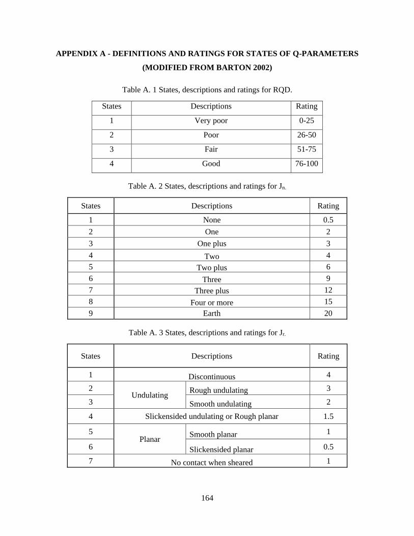
164
APPENDIX A - DEFINITIONS AND RATINGS FOR STATES OF Q-PARAMETERS
(MODIFIED FROM BARTON 2002)
Table A. 1 States, descriptions and ratings for RQD.
States Descriptions Rating
1 Very poor 0-25
2 Poor 26-50
3 Fair 51-75
4 Good 76-100
Table A. 2 States, descriptions and ratings for Jn.
States Descriptions Rating
1 None 0.5
2 One 2
3 One plus 3
4 Two 4
5 Two plus 6
6 Three 9
7 Three plus 12
8 Four or more 15
9 Earth 20
Table A. 3 States, descriptions and ratings for Jr.
States Descriptions Rating
1 Discontinuous 4
2 Undulating
Rough undulating 3
3 Smooth undulating 2
4 Slickensided undulating or Rough planar 1.5
5 Planar
Smooth planar 1
6 Slickensided planar 0.5
7 No contact when sheared 1

165
Table A. 4 States, descriptions and ratings for Ja.
States Descriptions Rating
1
No fills
Healed 0.75
2 Unaltered joint wall 1
3 Slightly altered wall 2
4 Coated non-softening 3
5 Coated softening or disintegrated sandy particles 4
6 Thin
fills
Thin non-softening clay fillings 6
7 Thin softening clay fillings 8
8 Thin swelling clays 12
9 Thick
fills
Thick, continuous; clay band; medium to low over-
consolidated 13
10 Thick, continuous; clay band; swelling clay 20
Table A. 5 States, descriptions and ratings for Jw.
States Descriptions Approx. water
press. (kg/cm2) Rating
1 Dry <1 1
2 Wet 1~2.5 0.66
3 High pressure in unfilled joints 2.5~10 0.5
4 High pressure with fillings outwash 2.5~10 0.33
5 Exc. inflows with decay >10 0.1
6 Exc. inflows without decay >10 0.05
Table A. 6 States, descriptions and ratings for SRF.
States Descriptions Sigma c/Sigma 1 Rating
1 Multiple clay zones 10
2 Multiple non-clay zones 7.5
3 Single weak zone (Depth<50m) or heavily jointed 5
4 Single weak zone (Depth>50m) or low stress(>200) 2.5
5 Medium stress 200-10 1
6 High stress with tight structure 10~5 2
7 Moderate slabbing 5~3 50
8 Slabbing and rock burst 3~2 200
9 Heavy rock burst <2 400
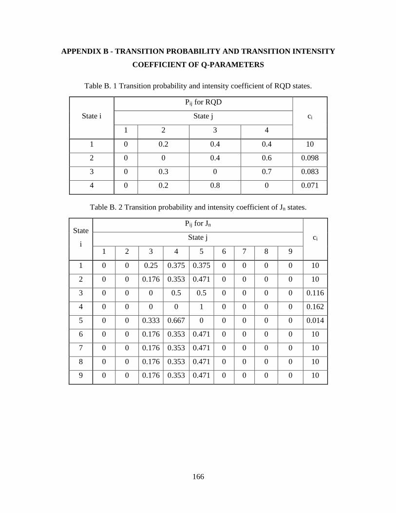
166
APPENDIX B - TRANSITION PROBABILITY AND TRANSITION INTENSITY
COEFFICIENT OF Q-PARAMETERS
Table B. 1 Transition probability and intensity coefficient of RQD states.
State i
Pij for RQD
ci State j
1 2 3 4
1 0 0.2 0.4 0.4 10
2 0 0 0.4 0.6 0.098
3 0 0.3 0 0.7 0.083
4 0 0.2 0.8 0 0.071
Table B. 2 Transition probability and intensity coefficient of Jn states.
State
i
Pij for Jn
ci State j
1 2 3 4 5 6 7 8 9
1 0 0 0.25 0.375 0.375 0 0 0 0 10
2 0 0 0.176 0.353 0.471 0 0 0 0 10
3 0 0 0 0.5 0.5 0 0 0 0 0.116
4 0 0 0 0 1 0 0 0 0 0.162
5 0 0 0.333 0.667 0 0 0 0 0 0.014
6 0 0 0.176 0.353 0.471 0 0 0 0 10
7 0 0 0.176 0.353 0.471 0 0 0 0 10
8 0 0 0.176 0.353 0.471 0 0 0 0 10
9 0 0 0.176 0.353 0.471 0 0 0 0 10
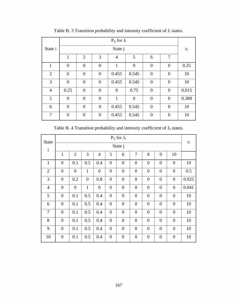
167
Table B. 3 Transition probability and intensity coefficient of Jr states.
State i
Pij for Jr
ci State j
1 2 3 4 5 6 7
1 0 0 0 1 0 0 0 0.25
2 0 0 0 0.455 0.545 0 0 10
3 0 0 0 0.455 0.545 0 0 10
4 0.25 0 0 0 0.75 0 0 0.015
5 0 0 0 1 0 0 0 0.389
6 0 0 0 0.455 0.545 0 0 10
7 0 0 0 0.455 0.545 0 0 10
Table B. 4 Transition probability and intensity coefficient of Ja states.
State
i
Pij for Ja ci
State j
1 2 3 4 5 6 7 8 9 10
1 0 0.1 0.5 0.4 0 0 0 0 0 0 10
2 0 0 1 0 0 0 0 0 0 0 0.5
3 0 0.2 0 0.8 0 0 0 0 0 0 0.025
4 0 0 1 0 0 0 0 0 0 0 0.041
5 0 0.1 0.5 0.4 0 0 0 0 0 0 10
6 0 0.1 0.5 0.4 0 0 0 0 0 0 10
7 0 0.1 0.5 0.4 0 0 0 0 0 0 10
8 0 0.1 0.5 0.4 0 0 0 0 0 0 10
9 0 0.1 0.5 0.4 0 0 0 0 0 0 10
10 0 0.1 0.5 0.4 0 0 0 0 0 0 10
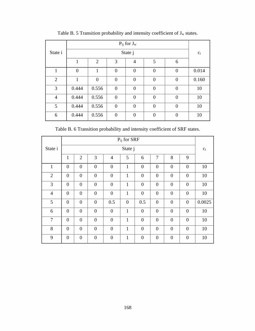
168
Table B. 5 Transition probability and intensity coefficient of Jw states.
State i
Pij for Jw
ci State j
1 2 3 4 5 6
1 0 1 0 0 0 0 0.014
2 1 0 0 0 0 0 0.160
3 0.444 0.556 0 0 0 0 10
4 0.444 0.556 0 0 0 0 10
5 0.444 0.556 0 0 0 0 10
6 0.444 0.556 0 0 0 0 10
Table B. 6 Transition probability and intensity coefficient of SRF states.
State i
Pij for SRF
ci State j
1 2 3 4 5 6 7 8 9
1 0 0 0 0 1 0 0 0 0 10
2 0 0 0 0 1 0 0 0 0 10
3 0 0 0 0 1 0 0 0 0 10
4 0 0 0 0 1 0 0 0 0 10
5 0 0 0 0.5 0 0.5 0 0 0 0.0025
6 0 0 0 0 1 0 0 0 0 10
7 0 0 0 0 1 0 0 0 0 10
8 0 0 0 0 1 0 0 0 0 10
9 0 0 0 0 1 0 0 0 0 10
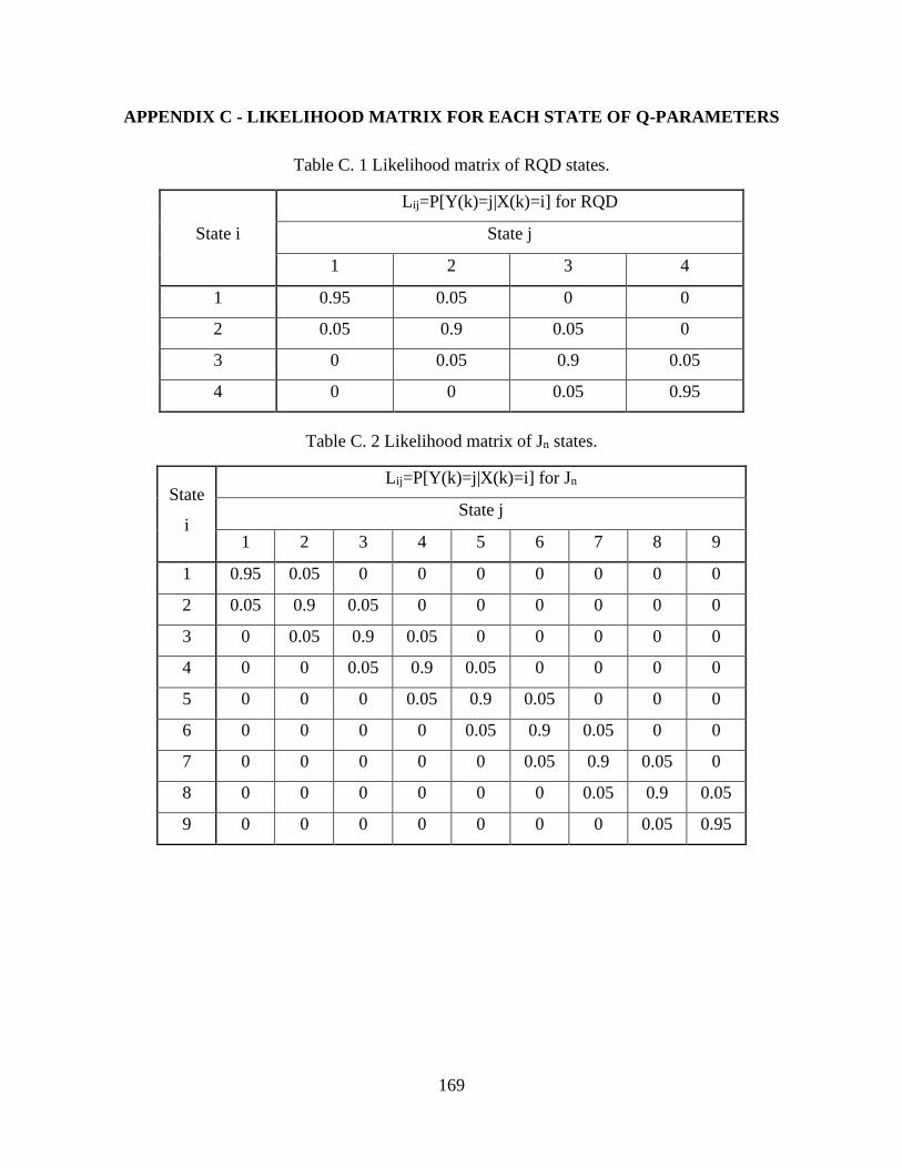
169
APPENDIX C - LIKELIHOOD MATRIX FOR EACH STATE OF Q-PARAMETERS
Table C. 1 Likelihood matrix of RQD states.
State i
Lij=P[Y(k)=j|X(k)=i] for RQD
State j
1 2 3 4
1 0.95 0.05 0 0
2 0.05 0.9 0.05 0
3 0 0.05 0.9 0.05
4 0 0 0.05 0.95
Table C. 2 Likelihood matrix of Jn states.
State
i
Lij=P[Y(k)=j|X(k)=i] for Jn
State j
1 2 3 4 5 6 7 8 9
1 0.95 0.05 0 0 0 0 0 0 0
2 0.05 0.9 0.05 0 0 0 0 0 0
3 0 0.05 0.9 0.05 0 0 0 0 0
4 0 0 0.05 0.9 0.05 0 0 0 0
5 0 0 0 0.05 0.9 0.05 0 0 0
6 0 0 0 0 0.05 0.9 0.05 0 0
7 0 0 0 0 0 0.05 0.9 0.05 0
8 0 0 0 0 0 0 0.05 0.9 0.05
9 0 0 0 0 0 0 0 0.05 0.95
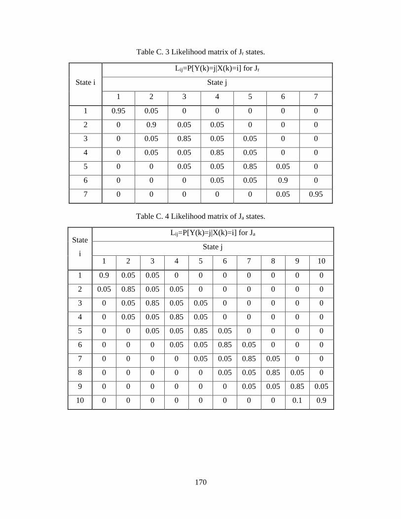
170
Table C. 3 Likelihood matrix of Jr states.
State i
Lij=P[Y(k)=j|X(k)=i] for Jr
State j
1 2 3 4 5 6 7
1 0.95 0.05 0 0 0 0 0
2 0 0.9 0.05 0.05 0 0 0
3 0 0.05 0.85 0.05 0.05 0 0
4 0 0.05 0.05 0.85 0.05 0 0
5 0 0 0.05 0.05 0.85 0.05 0
6 0 0 0 0.05 0.05 0.9 0
7 0 0 0 0 0 0.05 0.95
Table C. 4 Likelihood matrix of Ja states.
State
i
Lij=P[Y(k)=j|X(k)=i] for Ja
State j
1 2 3 4 5 6 7 8 9 10
1 0.9 0.05 0.05 0 0 0 0 0 0 0
2 0.05 0.85 0.05 0.05 0 0 0 0 0 0
3 0 0.05 0.85 0.05 0.05 0 0 0 0 0
4 0 0.05 0.05 0.85 0.05 0 0 0 0 0
5 0 0 0.05 0.05 0.85 0.05 0 0 0 0
6 0 0 0 0.05 0.05 0.85 0.05 0 0 0
7 0 0 0 0 0.05 0.05 0.85 0.05 0 0
8 0 0 0 0 0 0.05 0.05 0.85 0.05 0
9 0 0 0 0 0 0 0.05 0.05 0.85 0.05
10 0 0 0 0 0 0 0 0 0.1 0.9
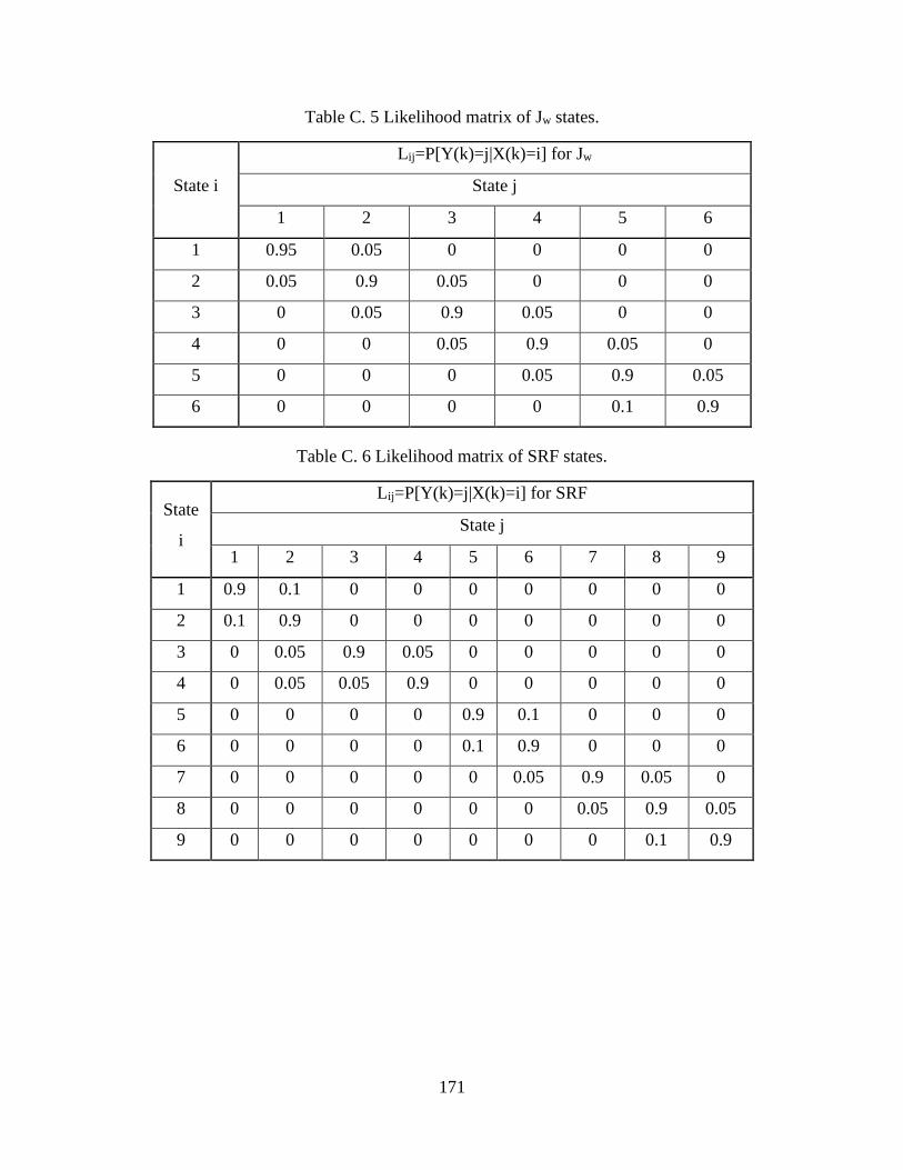
171
Table C. 5 Likelihood matrix of Jw states.
State i
Lij=P[Y(k)=j|X(k)=i] for Jw
State j
1 2 3 4 5 6
1 0.95 0.05 0 0 0 0
2 0.05 0.9 0.05 0 0 0
3 0 0.05 0.9 0.05 0 0
4 0 0 0.05 0.9 0.05 0
5 0 0 0 0.05 0.9 0.05
6 0 0 0 0 0.1 0.9
Table C. 6 Likelihood matrix of SRF states.
State
i
Lij=P[Y(k)=j|X(k)=i] for SRF
State j
1 2 3 4 5 6 7 8 9
1 0.9 0.1 0 0 0 0 0 0 0
2 0.1 0.9 0 0 0 0 0 0 0
3 0 0.05 0.9 0.05 0 0 0 0 0
4 0 0.05 0.05 0.9 0 0 0 0 0
5 0 0 0 0 0.9 0.1 0 0 0
6 0 0 0 0 0.1 0.9 0 0 0
7 0 0 0 0 0 0.05 0.9 0.05 0
8 0 0 0 0 0 0 0.05 0.9 0.05
9 0 0 0 0 0 0 0 0.1 0.9
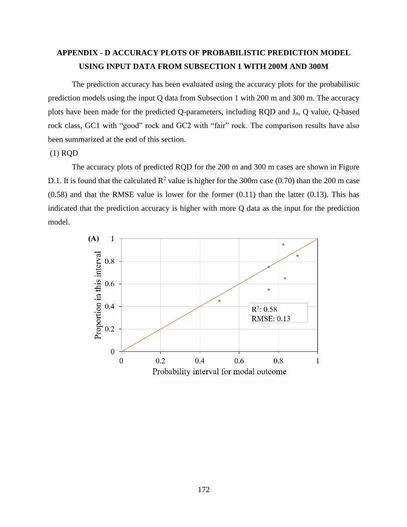
172
APPENDIX - D ACCURACY PLOTS OF PROBABILISTIC PREDICTION MODEL
USING INPUT DATA FROM SUBSECTION 1 WITH 200M AND 300M
The prediction accuracy has been evaluated using the accuracy plots for the probabilistic
prediction models using the input Q data from Subsection 1 with 200 m and 300 m. The accuracy
plots have been made for the predicted Q-parameters, including RQD and Jn, Q value, Q-based
rock class, GC1 with “good” rock and GC2 with “fair” rock. The comparison results have also
been summarized at the end of this section.
(1) RQD
The accuracy plots of predicted RQD for the 200 m and 300 m cases are shown in Figure
D.1. It is found that the calculated R2 value is higher for the 300m case (0.70) than the 200 m case
(0.58) and that the RMSE value is lower for the former (0.11) than the latter (0.13). This has
indicated that the prediction accuracy is higher with more Q data as the input for the prediction
model.

173
Figure D. 1 Accuracy plots for predicted RQD: (A): the 200 m case; (B): the 300 m case
(2) Jn
The accuracy plots for the predicted Jn are demonstrated in Figure D.2. Similar to the
predicted results for RQD, the prediction accuracy is higher for the 300 m case than the 200 m
case. However, it is seen that the R2 values for the predicted Jn are lower than those for the RQD
and the RMSE values are higher for the former compared to the latter. This reveals the predicted
RQD has higher prediction accuracy than the predicted Jn results, which is consistent with the
results derived from the 400 m case.
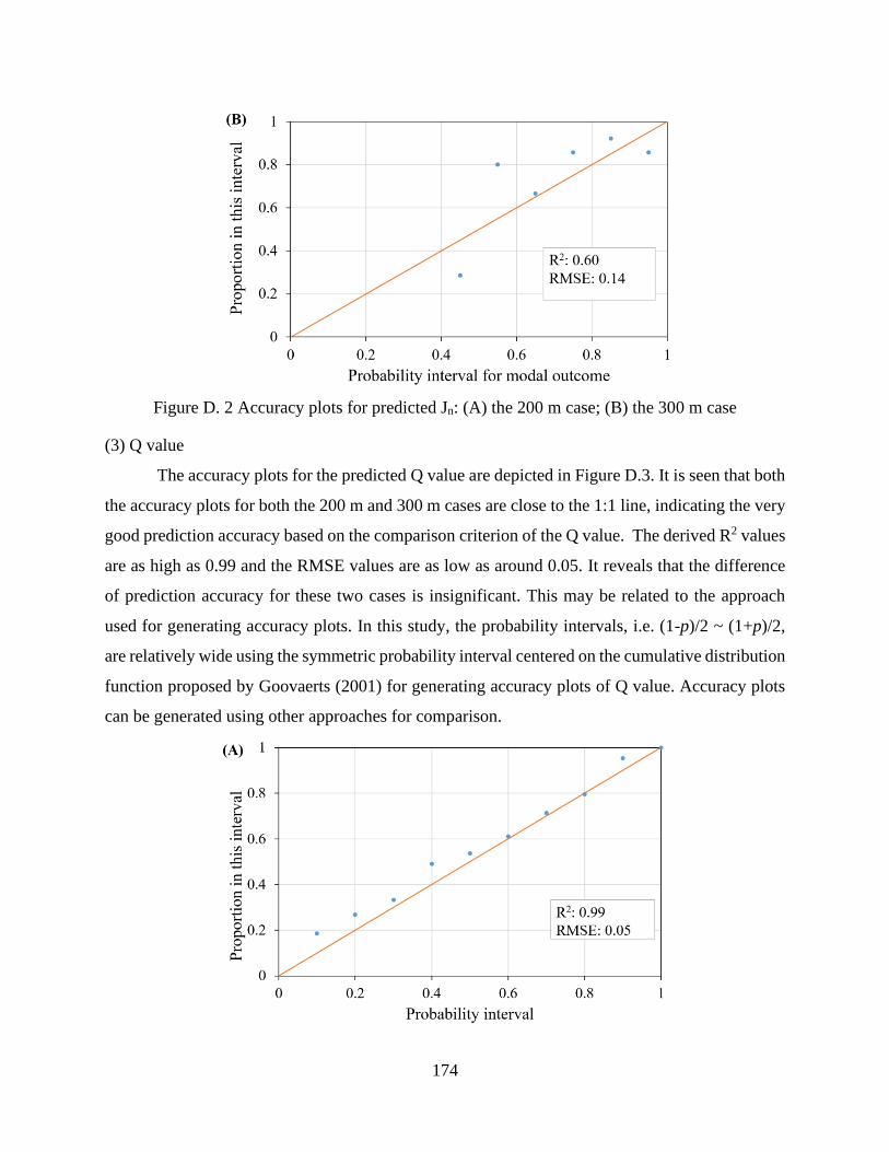
174
Figure D. 2 Accuracy plots for predicted Jn: (A) the 200 m case; (B) the 300 m case
(3) Q value
The accuracy plots for the predicted Q value are depicted in Figure D.3. It is seen that both
the accuracy plots for both the 200 m and 300 m cases are close to the 1:1 line, indicating the very
good prediction accuracy based on the comparison criterion of the Q value. The derived R2 values
are as high as 0.99 and the RMSE values are as low as around 0.05. It reveals that the difference
of prediction accuracy for these two cases is insignificant. This may be related to the approach
used for generating accuracy plots. In this study, the probability intervals, i.e. (1-p)/2 ~ (1+p)/2,
are relatively wide using the symmetric probability interval centered on the cumulative distribution
function proposed by Goovaerts (2001) for generating accuracy plots of Q value. Accuracy plots
can be generated using other approaches for comparison.
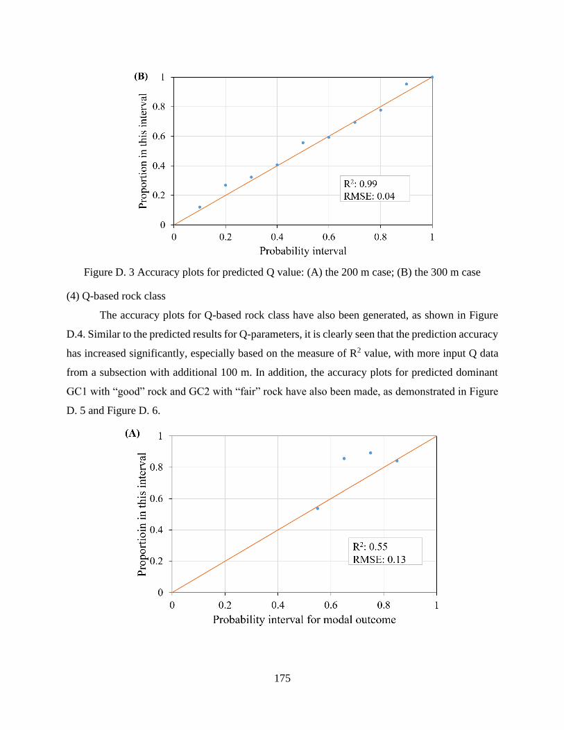
175
Figure D. 3 Accuracy plots for predicted Q value: (A) the 200 m case; (B) the 300 m case
(4) Q-based rock class
The accuracy plots for Q-based rock class have also been generated, as shown in Figure
D.4. Similar to the predicted results for Q-parameters, it is clearly seen that the prediction accuracy
has increased significantly, especially based on the measure of R2 value, with more input Q data
from a subsection with additional 100 m. In addition, the accuracy plots for predicted dominant
GC1 with “good” rock and GC2 with “fair” rock have also been made, as demonstrated in Figure
D. 5 and Figure D. 6.
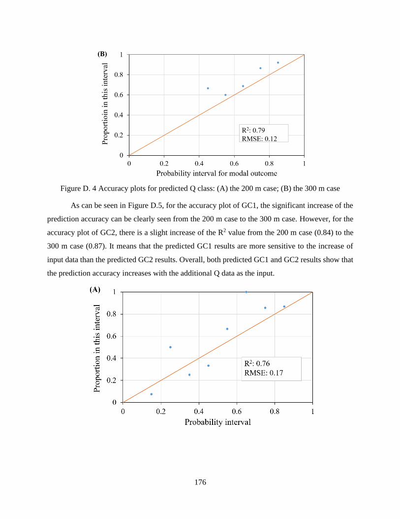
176
Figure D. 4 Accuracy plots for predicted Q class: (A) the 200 m case; (B) the 300 m case
As can be seen in Figure D.5, for the accuracy plot of GC1, the significant increase of the
prediction accuracy can be clearly seen from the 200 m case to the 300 m case. However, for the
accuracy plot of GC2, there is a slight increase of the R2 value from the 200 m case (0.84) to the
300 m case (0.87). It means that the predicted GC1 results are more sensitive to the increase of
input data than the predicted GC2 results. Overall, both predicted GC1 and GC2 results show that
the prediction accuracy increases with the additional Q data as the input.
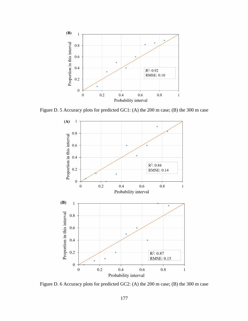
177
Figure D. 5 Accuracy plots for predicted GC1: (A) the 200 m case; (B) the 300 m case
Figure D. 6 Accuracy plots for predicted GC2: (A) the 200 m case; (B) the 300 m case
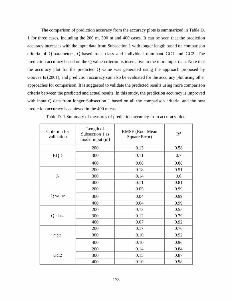
178
The comparison of prediction accuracy from the accuracy plots is summarized in Table D.
1 for three cases, including the 200 m, 300 m and 400 cases. It can be seen that the prediction
accuracy increases with the input data from Subsection 1 with longer length based on comparison
criteria of Q-parameters, Q-based rock class and individual dominant GC1 and GC2. The
prediction accuracy based on the Q value criterion is insensitive to the more input data. Note that
the accuracy plot for the predicted Q value was generated using the approach proposed by
Goovaerts (2001), and prediction accuracy can also be evaluated for the accuracy plot using other
approaches for comparison. It is suggested to validate the predicted results using more comparison
criteria between the predicted and actual results. In this study, the prediction accuracy is improved
with input Q data from longer Subsection 1 based on all the comparison criteria, and the best
prediction accuracy is achieved in the 400 m case.
Table D. 1 Summary of measures of prediction accuracy from accuracy plots
Criterion for
validation
Length of
Subsection 1 as
model input (m)
RMSE (Root Mean
Square Error) R2
RQD
200 0.13 0.58
300 0.11 0.7
400 0.08 0.88
Jn
200 0.18 0.51
300 0.14 0.6
400 0.11 0.81
Q value
200 0.05 0.99
300 0.04 0.99
400 0.04 0.99
Q class
200 0.13 0.55
300 0.12 0.79
400 0.07 0.92
GC1
200 0.17 0.76
300 0.10 0.92
400 0.10 0.96
GC2
200 0.14 0.84
300 0.15 0.87
400 0.10 0.98
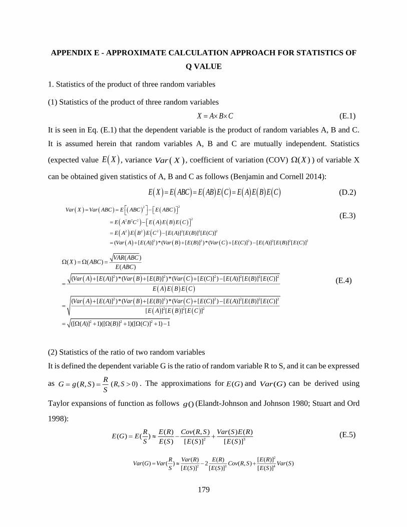
179
APPENDIX E - APPROXIMATE CALCULATION APPROACH FOR STATISTICS OF
Q VALUE
1. Statistics of the product of three random variables
(1) Statistics of the product of three random variables
X A B C= (E.1)
It is seen in Eq. (E.1) that the dependent variable is the product of random variables A, B and C.
It is assumed herein that random variables A, B and C are mutually independent. Statistics
(expected value ( )E X , variance ( )Var X , coefficient of variation (COV) ( )X ) of variable X
can be obtained given statistics of A, B and C as follows (Benjamin and Cornell 2014):
( ) ( ) ( ) ( ) ( ) ( ) ( )E X E ABC E AB E C E A E B E C= = = (D.2)
( ) ( ) ( ) ( )
( ) ( ) ( ) ( )
( ) ( ) ( )( ) ( )
22
22 2 2
2 2 2 2 2 2
2
] [ ( )
(
[ ( )] [ ( )
[ ( )] )*(
]
Var X Var ABC E ABC E ABC
E A B C E A E B E C
E A E B E C E A
Var A E
E E
A Var
B
B
C
= = −
= −
= −
= + ( ) 22 22 2[ ( )] )*( [ ( )] ) ] [ ( )] [ ( )[ ( ) ]E B Var EC E B EC E A C+ + −
(E.3)
( ) ( ) ( )
( ) ( ) ( )
( ) ( ) ( )
( ) ( ) ( )
2 2 2 2
2 2
2 2
2 2
2 2
2 2
2
2
( [ ( )] )*( [ ( )] )*( [ ( )] ) [ ( )
( [ ( )] )
( )( ) ( )
( )
] [ ( )] [ ( )]
] [ ( )] [ ( )]
] [ ] [ ]
([ (
*( [ ( )] )*(
)] 1)([ (
[ ( )] ) [ ( )
[
)]
Var A E A Var B E B Var E C E A
E A E B E C
Var A E A V
VAR ABCX ABC
E ABC
C E B E C
C E B E Car B E B Var E C E A
E A E B E C
A B
+ + + −
+ + +
= =
=
=
=
−
+ 2 21)([ ( )] 1) 1C+ + −
(E.4)
(2) Statistics of the ratio of two random variables
It is defined the dependent variable G is the ratio of random variable R to S, and it can be expressed
as ( , )R
G g R SS
= = ( , 0)R S . The approximations for ( )E G and ( )Var G can be derived using
Taylor expansions of function as follows ()g (Elandt-Johnson and Johnson 1980; Stuart and Ord
1998):
2 3
( ) ( , ) ( ) ( )( ) ( )
( ) [ ( )] [ ( )]
R E R Cov R S Var S E RE G E
S E S E S E S= − + (E.5)
2
2 3 4
( ) ( ) [ ( )]( ) ( ) 2 ( , ) ( )
[ ( )] [ ( )] [ ( )]
R Var R E R E RVar G Var Cov R S Var S
S E S E S E S= − +
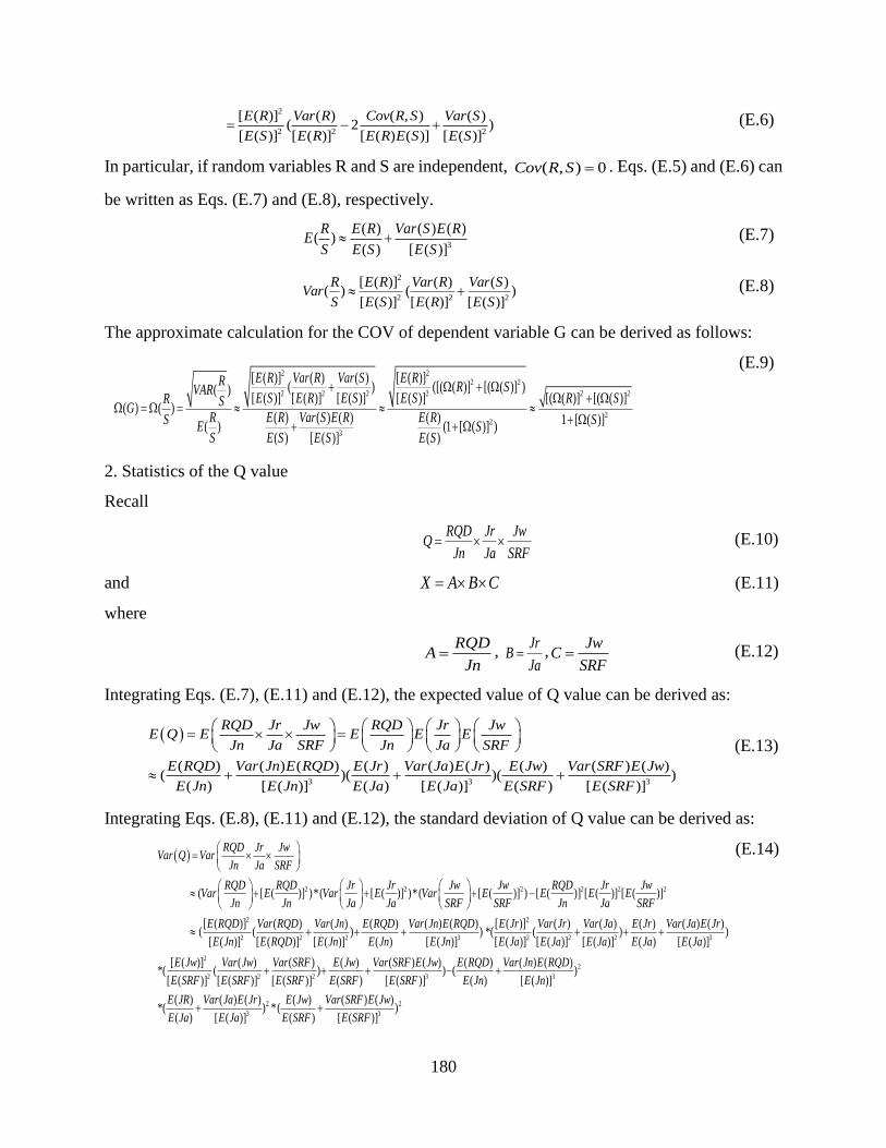
180
2
2 2 2
[ ( )] ( ) ( , ) ( )( 2 )
[ ( )] [ ( )] [ ( ) ( )] [ ( )]
E R Var R Cov R S Var S
E S E R E R E S E S= − + (E.6)
In particular, if random variables R and S are independent, ( , ) 0Cov R S = . Eqs. (E.5) and (E.6) can
be written as Eqs. (E.7) and (E.8), respectively.
3
( ) ( ) ( )( )
( ) [ ( )]
R E R Var S E RE
S E S E S + (E.7)
2
2 2 2
[ ( )] ( ) ( )( ) ( )
[ ( )] [ ( )] [ ( )]
R E R Var R Var SVar
S E S E R E S + (E.8)
The approximate calculation for the COV of dependent variable G can be derived as follows:
2 22 2
2 2 2 2 2 2
22
3
[ ( )] ( ) ( ) [ ( )]( ) ([( ( )] [( ( )] )( )
[ ( )] [ ( )] [ ( )] [ ( )] [( ( )] [( ( )]( ) ( )
( ) ( ) ( ) ( ) 1 [ ( )]( ) (1 [ ( )] )
( ) [ ( )] ( )
E R Var R Var S E RR R SVARE S E R E S E S R SR S
GR E R Var S E R E RS S
E SS E S E S E S
+ + +
= = +
+ +
(E.9)
2. Statistics of the Q value
Recall
RQD Jr JwQ
Jn Ja SRF= (E.10)
and X A B C= (E.11)
where
RQDA
Jn= ,
JrB
Ja= ,
JwC
SRF= (E.12)
Integrating Eqs. (E.7), (E.11) and (E.12), the expected value of Q value can be derived as:
( )
3 3 3
( ) ( ) ( ) ( ) ( ) ( ) ( ) ( ) ( )( )( )( )
( ) [ ( )] ( ) [ ( )] ( ) [ ( )]
RQD Jr Jw RQD Jr Jw
Jn Ja SRF Jn Ja SRF
E RQD Var Jn E RQD E Jr Var Ja E Jr E Jw Var SRF E Jw
E Jn E Jn E Ja E Ja E SRF E SR
E E E E
F
Q E
+ + +
= = (E.13)
Integrating Eqs. (E.8), (E.11) and (E.12), the standard deviation of Q value can be derived as:
( )
2 2 2 2 2
2
2
2 ( [ ( )] )*( [ ( )] )*( [ ( )] ) [ ( )
] [ ( )] [ ( )]
[ ( )
] ((
[ ((
)]
RQD Jr Jw
Jn Ja SRF
RQD RQD Jr Jr Jw Jw RQD Jr JwE E
Jn Jn Ja Ja SRF SRF Jn Ja SR
Var Q Var
Var E Var E Var EF
E RQD r
E n
E
Va
J
=
+ + + −
2
2 2 3 2 2 2 3
2
2 2
) ( ) ( ) ( ) ( ) [ ( )] ( ) ( ) ( ) ( ) ( )) ) ( ) )
[ ( )] [ ( )] ( ) [ ( )] [ ( )] [ ( )] [ ( )] ( )
[ ( )]
[ ( )] ( ) ( )(
[ ( )] [ ( )]
*(
*( [
RQD Var Jn E RQD Var Jn E RQD E Jr Var Jr Var Ja E Jr Var Ja E Jr
E RQD E Jn E Jn E Jn E Ja E Ja E Ja E Ja E Ja
E Jw Var Jw Var SRF
E SRF E SRF
+ + +
+
++ +
2
2 3 3
2 2
3 3
(( ) ( ) ( ) ( ) ( ) ( )
) ) )( )] ( ) [ ( )] ( ) [ ( )]
( ) ( ) ( ) ( ) ( ) ( )* ) * )
( ) [ ( )]( (
]
( ) [ ( )
E Jw Var SRF E Jw E RQD Var Jn E RQD
E SRF E SRF E SRF E Jn E Jn
E JR Var Ja E Jr E Jw Var SRF E Jw
E Ja E Ja E SRF E SRF
+ +
+ +
+ −
(E.14)
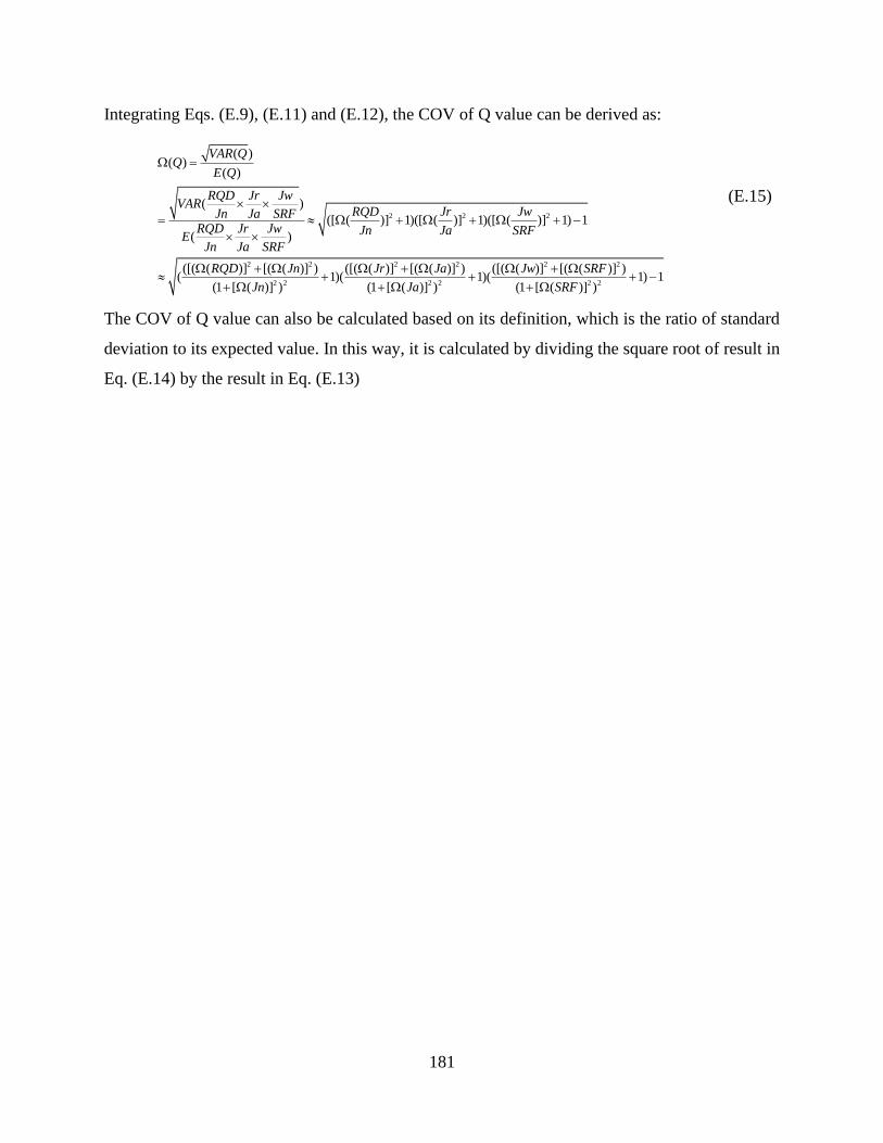
181
Integrating Eqs. (E.9), (E.11) and (E.12), the COV of Q value can be derived as:
2 2 2
2 2 2 2 2
2 2 2 2
( )( )
( )
( )
([ ( )] 1)([ ( )] 1)([ ( )] 1) 1
( )
([( ( )] [( ( )] ) ([( ( )] [( ( )] ) ([( ( )] [( (( 1)( 1)(
(1 [ ( )] ) (1 [ ( )] )
VAR QQ
E Q
RQD Jr JwVAR
RQD Jr JwJn Ja SRFRQD Jr Jw Jn Ja SRF
EJn Ja SRF
RQD Jn Jr Ja Jw SRF
Jn Ja
=
= + + + −
+ + + + +
+ +
2
2 2
)] )1) 1
(1 [ ( )] )SRF+ −
+
(E.15)
The COV of Q value can also be calculated based on its definition, which is the ratio of standard
deviation to its expected value. In this way, it is calculated by dividing the square root of result in
Eq. (E.14) by the result in Eq. (E.13)
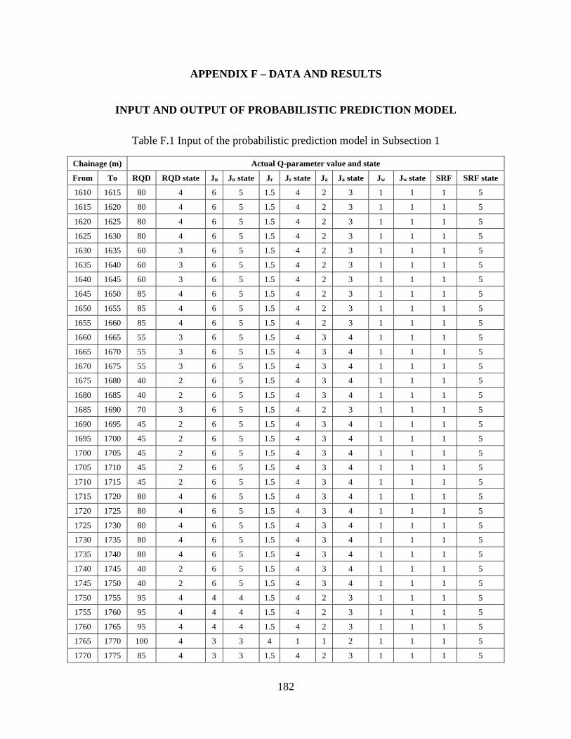
182
APPENDIX F – DATA AND RESULTS
INPUT AND OUTPUT OF PROBABILISTIC PREDICTION MODEL
Table F.1 Input of the probabilistic prediction model in Subsection 1
Chainage (m) Actual Q-parameter value and state
From To RQD RQD state Jn Jn state Jr Jr state Ja Ja state Jw Jw state SRF SRF state
1610 1615 80 4 6 5 1.5 4 2 3 1 1 1 5
1615 1620 80 4 6 5 1.5 4 2 3 1 1 1 5
1620 1625 80 4 6 5 1.5 4 2 3 1 1 1 5
1625 1630 80 4 6 5 1.5 4 2 3 1 1 1 5
1630 1635 60 3 6 5 1.5 4 2 3 1 1 1 5
1635 1640 60 3 6 5 1.5 4 2 3 1 1 1 5
1640 1645 60 3 6 5 1.5 4 2 3 1 1 1 5
1645 1650 85 4 6 5 1.5 4 2 3 1 1 1 5
1650 1655 85 4 6 5 1.5 4 2 3 1 1 1 5
1655 1660 85 4 6 5 1.5 4 2 3 1 1 1 5
1660 1665 55 3 6 5 1.5 4 3 4 1 1 1 5
1665 1670 55 3 6 5 1.5 4 3 4 1 1 1 5
1670 1675 55 3 6 5 1.5 4 3 4 1 1 1 5
1675 1680 40 2 6 5 1.5 4 3 4 1 1 1 5
1680 1685 40 2 6 5 1.5 4 3 4 1 1 1 5
1685 1690 70 3 6 5 1.5 4 2 3 1 1 1 5
1690 1695 45 2 6 5 1.5 4 3 4 1 1 1 5
1695 1700 45 2 6 5 1.5 4 3 4 1 1 1 5
1700 1705 45 2 6 5 1.5 4 3 4 1 1 1 5
1705 1710 45 2 6 5 1.5 4 3 4 1 1 1 5
1710 1715 45 2 6 5 1.5 4 3 4 1 1 1 5
1715 1720 80 4 6 5 1.5 4 3 4 1 1 1 5
1720 1725 80 4 6 5 1.5 4 3 4 1 1 1 5
1725 1730 80 4 6 5 1.5 4 3 4 1 1 1 5
1730 1735 80 4 6 5 1.5 4 3 4 1 1 1 5
1735 1740 80 4 6 5 1.5 4 3 4 1 1 1 5
1740 1745 40 2 6 5 1.5 4 3 4 1 1 1 5
1745 1750 40 2 6 5 1.5 4 3 4 1 1 1 5
1750 1755 95 4 4 4 1.5 4 2 3 1 1 1 5
1755 1760 95 4 4 4 1.5 4 2 3 1 1 1 5
1760 1765 95 4 4 4 1.5 4 2 3 1 1 1 5
1765 1770 100 4 3 3 4 1 1 2 1 1 1 5
1770 1775 85 4 3 3 1.5 4 2 3 1 1 1 5
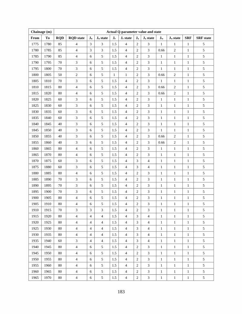
183
Chainage (m) Actual Q-parameter value and state
From To RQD RQD state Jn Jn state Jr Jr state Ja Ja state Jw Jw state SRF SRF state
1775 1780 85 4 3 3 1.5 4 2 3 1 1 1 5
1780 1785 85 4 3 3 1.5 4 2 3 0.66 2 1 5
1785 1790 85 4 6 5 1.5 4 2 3 1 1 1 5
1790 1795 70 3 6 5 1.5 4 2 3 1 1 1 5
1795 1800 70 3 6 5 1.5 4 2 3 1 1 1 5
1800 1805 50 2 6 5 1 1 2 3 0.66 2 1 5
1805 1810 70 3 6 5 1.5 4 2 3 1 1 1 5
1810 1815 80 4 6 5 1.5 4 2 3 0.66 2 1 5
1815 1820 80 4 6 5 1.5 4 2 3 0.66 2 1 5
1820 1825 60 3 6 5 1.5 4 2 3 1 1 1 5
1825 1830 60 3 6 5 1.5 4 2 3 1 1 1 5
1830 1835 60 3 6 5 1.5 4 2 3 1 1 1 5
1835 1840 60 3 6 5 1.5 4 2 3 1 1 1 5
1840 1845 40 3 6 5 1.5 4 2 3 1 1 1 5
1845 1850 40 3 6 5 1.5 4 2 3 1 1 1 5
1850 1855 40 3 6 5 1.5 4 2 3 0.66 2 1 5
1855 1860 40 3 6 5 1.5 4 2 3 0.66 2 1 5
1860 1865 80 4 6 5 1.5 4 2 3 1 1 1 5
1865 1870 80 4 6 5 1.5 4 2 3 1 1 1 5
1870 1875 60 3 6 5 1.5 4 3 4 1 1 1 5
1875 1880 60 3 6 5 1.5 4 3 4 1 1 1 5
1880 1885 80 4 6 5 1.5 4 2 3 1 1 1 5
1885 1890 70 3 6 5 1.5 4 2 3 1 1 1 5
1890 1895 70 3 6 5 1.5 4 2 3 1 1 1 5
1895 1900 70 3 6 5 1.5 4 2 3 1 1 1 5
1900 1905 80 4 6 5 1.5 4 2 3 1 1 1 5
1905 1910 80 4 6 5 1.5 4 2 3 1 1 1 5
1910 1915 70 3 3 3 1.5 4 2 3 1 1 1 5
1915 1920 80 4 4 4 1.5 4 3 4 1 1 1 5
1920 1925 80 4 4 4 1.5 4 3 4 1 1 1 5
1925 1930 80 4 4 4 1.5 4 3 4 1 1 1 5
1930 1935 80 4 4 4 1.5 4 3 4 1 1 1 5
1935 1940 60 3 4 4 1.5 4 3 4 1 1 1 5
1940 1945 80 4 6 5 1.5 4 2 3 1 1 1 5
1945 1950 80 4 6 5 1.5 4 2 3 1 1 1 5
1950 1955 80 4 6 5 1.5 4 2 3 1 1 1 5
1955 1960 80 4 6 5 1.5 4 2 3 1 1 1 5
1960 1965 80 4 6 5 1.5 4 2 3 1 1 1 5
1965 1970 80 4 6 5 1.5 4 2 3 1 1 1 5
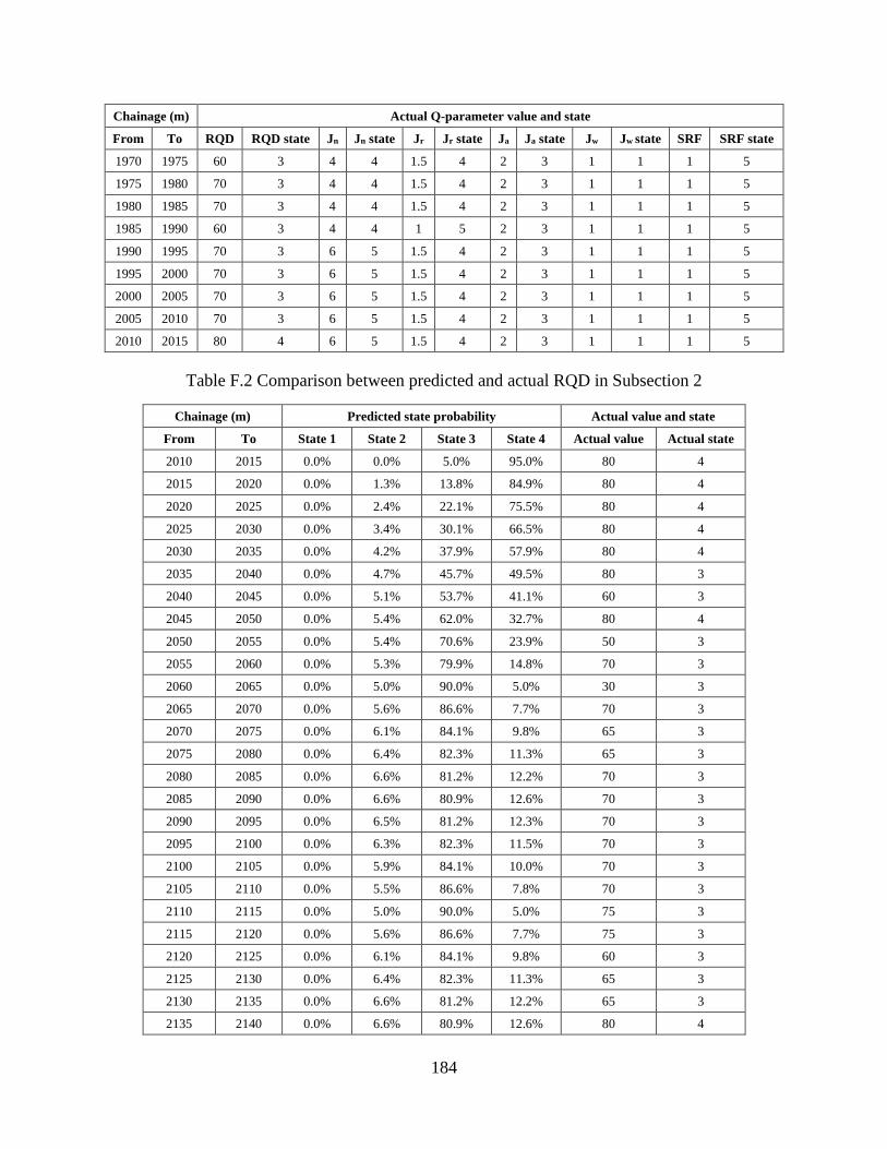
184
Chainage (m) Actual Q-parameter value and state
From To RQD RQD state Jn Jn state Jr Jr state Ja Ja state Jw Jw state SRF SRF state
1970 1975 60 3 4 4 1.5 4 2 3 1 1 1 5
1975 1980 70 3 4 4 1.5 4 2 3 1 1 1 5
1980 1985 70 3 4 4 1.5 4 2 3 1 1 1 5
1985 1990 60 3 4 4 1 5 2 3 1 1 1 5
1990 1995 70 3 6 5 1.5 4 2 3 1 1 1 5
1995 2000 70 3 6 5 1.5 4 2 3 1 1 1 5
2000 2005 70 3 6 5 1.5 4 2 3 1 1 1 5
2005 2010 70 3 6 5 1.5 4 2 3 1 1 1 5
2010 2015 80 4 6 5 1.5 4 2 3 1 1 1 5
Table F.2 Comparison between predicted and actual RQD in Subsection 2
Chainage (m) Predicted state probability Actual value and state
From To State 1 State 2 State 3 State 4 Actual value Actual state
2010 2015 0.0% 0.0% 5.0% 95.0% 80 4
2015 2020 0.0% 1.3% 13.8% 84.9% 80 4
2020 2025 0.0% 2.4% 22.1% 75.5% 80 4
2025 2030 0.0% 3.4% 30.1% 66.5% 80 4
2030 2035 0.0% 4.2% 37.9% 57.9% 80 4
2035 2040 0.0% 4.7% 45.7% 49.5% 80 3
2040 2045 0.0% 5.1% 53.7% 41.1% 60 3
2045 2050 0.0% 5.4% 62.0% 32.7% 80 4
2050 2055 0.0% 5.4% 70.6% 23.9% 50 3
2055 2060 0.0% 5.3% 79.9% 14.8% 70 3
2060 2065 0.0% 5.0% 90.0% 5.0% 30 3
2065 2070 0.0% 5.6% 86.6% 7.7% 70 3
2070 2075 0.0% 6.1% 84.1% 9.8% 65 3
2075 2080 0.0% 6.4% 82.3% 11.3% 65 3
2080 2085 0.0% 6.6% 81.2% 12.2% 70 3
2085 2090 0.0% 6.6% 80.9% 12.6% 70 3
2090 2095 0.0% 6.5% 81.2% 12.3% 70 3
2095 2100 0.0% 6.3% 82.3% 11.5% 70 3
2100 2105 0.0% 5.9% 84.1% 10.0% 70 3
2105 2110 0.0% 5.5% 86.6% 7.8% 70 3
2110 2115 0.0% 5.0% 90.0% 5.0% 75 3
2115 2120 0.0% 5.6% 86.6% 7.7% 75 3
2120 2125 0.0% 6.1% 84.1% 9.8% 60 3
2125 2130 0.0% 6.4% 82.3% 11.3% 65 3
2130 2135 0.0% 6.6% 81.2% 12.2% 65 3
2135 2140 0.0% 6.6% 80.9% 12.6% 80 4
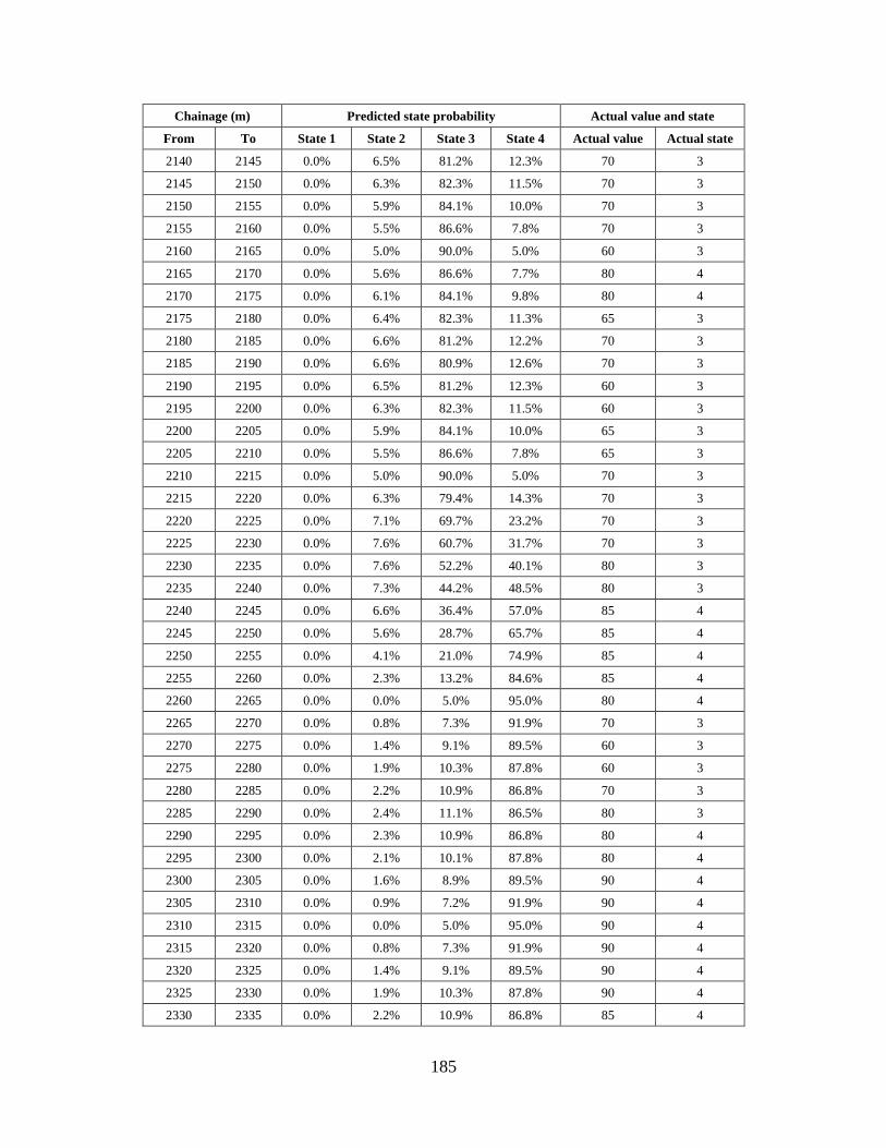
185
Chainage (m) Predicted state probability Actual value and state
From To State 1 State 2 State 3 State 4 Actual value Actual state
2140 2145 0.0% 6.5% 81.2% 12.3% 70 3
2145 2150 0.0% 6.3% 82.3% 11.5% 70 3
2150 2155 0.0% 5.9% 84.1% 10.0% 70 3
2155 2160 0.0% 5.5% 86.6% 7.8% 70 3
2160 2165 0.0% 5.0% 90.0% 5.0% 60 3
2165 2170 0.0% 5.6% 86.6% 7.7% 80 4
2170 2175 0.0% 6.1% 84.1% 9.8% 80 4
2175 2180 0.0% 6.4% 82.3% 11.3% 65 3
2180 2185 0.0% 6.6% 81.2% 12.2% 70 3
2185 2190 0.0% 6.6% 80.9% 12.6% 70 3
2190 2195 0.0% 6.5% 81.2% 12.3% 60 3
2195 2200 0.0% 6.3% 82.3% 11.5% 60 3
2200 2205 0.0% 5.9% 84.1% 10.0% 65 3
2205 2210 0.0% 5.5% 86.6% 7.8% 65 3
2210 2215 0.0% 5.0% 90.0% 5.0% 70 3
2215 2220 0.0% 6.3% 79.4% 14.3% 70 3
2220 2225 0.0% 7.1% 69.7% 23.2% 70 3
2225 2230 0.0% 7.6% 60.7% 31.7% 70 3
2230 2235 0.0% 7.6% 52.2% 40.1% 80 3
2235 2240 0.0% 7.3% 44.2% 48.5% 80 3
2240 2245 0.0% 6.6% 36.4% 57.0% 85 4
2245 2250 0.0% 5.6% 28.7% 65.7% 85 4
2250 2255 0.0% 4.1% 21.0% 74.9% 85 4
2255 2260 0.0% 2.3% 13.2% 84.6% 85 4
2260 2265 0.0% 0.0% 5.0% 95.0% 80 4
2265 2270 0.0% 0.8% 7.3% 91.9% 70 3
2270 2275 0.0% 1.4% 9.1% 89.5% 60 3
2275 2280 0.0% 1.9% 10.3% 87.8% 60 3
2280 2285 0.0% 2.2% 10.9% 86.8% 70 3
2285 2290 0.0% 2.4% 11.1% 86.5% 80 3
2290 2295 0.0% 2.3% 10.9% 86.8% 80 4
2295 2300 0.0% 2.1% 10.1% 87.8% 80 4
2300 2305 0.0% 1.6% 8.9% 89.5% 90 4
2305 2310 0.0% 0.9% 7.2% 91.9% 90 4
2310 2315 0.0% 0.0% 5.0% 95.0% 90 4
2315 2320 0.0% 0.8% 7.3% 91.9% 90 4
2320 2325 0.0% 1.4% 9.1% 89.5% 90 4
2325 2330 0.0% 1.9% 10.3% 87.8% 90 4
2330 2335 0.0% 2.2% 10.9% 86.8% 85 4
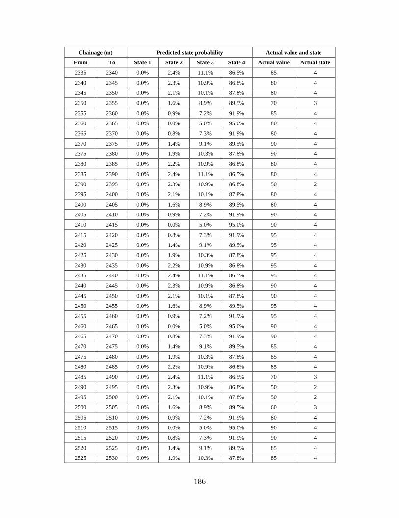
186
Chainage (m) Predicted state probability Actual value and state
From To State 1 State 2 State 3 State 4 Actual value Actual state
2335 2340 0.0% 2.4% 11.1% 86.5% 85 4
2340 2345 0.0% 2.3% 10.9% 86.8% 80 4
2345 2350 0.0% 2.1% 10.1% 87.8% 80 4
2350 2355 0.0% 1.6% 8.9% 89.5% 70 3
2355 2360 0.0% 0.9% 7.2% 91.9% 85 4
2360 2365 0.0% 0.0% 5.0% 95.0% 80 4
2365 2370 0.0% 0.8% 7.3% 91.9% 80 4
2370 2375 0.0% 1.4% 9.1% 89.5% 90 4
2375 2380 0.0% 1.9% 10.3% 87.8% 90 4
2380 2385 0.0% 2.2% 10.9% 86.8% 80 4
2385 2390 0.0% 2.4% 11.1% 86.5% 80 4
2390 2395 0.0% 2.3% 10.9% 86.8% 50 2
2395 2400 0.0% 2.1% 10.1% 87.8% 80 4
2400 2405 0.0% 1.6% 8.9% 89.5% 80 4
2405 2410 0.0% 0.9% 7.2% 91.9% 90 4
2410 2415 0.0% 0.0% 5.0% 95.0% 90 4
2415 2420 0.0% 0.8% 7.3% 91.9% 95 4
2420 2425 0.0% 1.4% 9.1% 89.5% 95 4
2425 2430 0.0% 1.9% 10.3% 87.8% 95 4
2430 2435 0.0% 2.2% 10.9% 86.8% 95 4
2435 2440 0.0% 2.4% 11.1% 86.5% 95 4
2440 2445 0.0% 2.3% 10.9% 86.8% 90 4
2445 2450 0.0% 2.1% 10.1% 87.8% 90 4
2450 2455 0.0% 1.6% 8.9% 89.5% 95 4
2455 2460 0.0% 0.9% 7.2% 91.9% 95 4
2460 2465 0.0% 0.0% 5.0% 95.0% 90 4
2465 2470 0.0% 0.8% 7.3% 91.9% 90 4
2470 2475 0.0% 1.4% 9.1% 89.5% 85 4
2475 2480 0.0% 1.9% 10.3% 87.8% 85 4
2480 2485 0.0% 2.2% 10.9% 86.8% 85 4
2485 2490 0.0% 2.4% 11.1% 86.5% 70 3
2490 2495 0.0% 2.3% 10.9% 86.8% 50 2
2495 2500 0.0% 2.1% 10.1% 87.8% 50 2
2500 2505 0.0% 1.6% 8.9% 89.5% 60 3
2505 2510 0.0% 0.9% 7.2% 91.9% 80 4
2510 2515 0.0% 0.0% 5.0% 95.0% 90 4
2515 2520 0.0% 0.8% 7.3% 91.9% 90 4
2520 2525 0.0% 1.4% 9.1% 89.5% 85 4
2525 2530 0.0% 1.9% 10.3% 87.8% 85 4
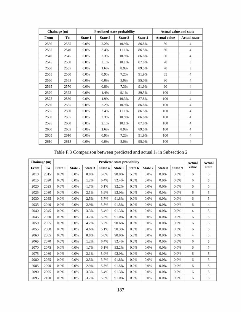
187
Chainage (m) Predicted state probability Actual value and state
From To State 1 State 2 State 3 State 4 Actual value Actual state
2530 2535 0.0% 2.2% 10.9% 86.8% 80 4
2535 2540 0.0% 2.4% 11.1% 86.5% 80 4
2540 2545 0.0% 2.3% 10.9% 86.8% 80 4
2545 2550 0.0% 2.1% 10.1% 87.8% 70 3
2550 2555 0.0% 1.6% 8.9% 89.5% 70 3
2555 2560 0.0% 0.9% 7.2% 91.9% 85 4
2560 2565 0.0% 0.0% 5.0% 95.0% 90 4
2565 2570 0.0% 0.8% 7.3% 91.9% 90 4
2570 2575 0.0% 1.4% 9.1% 89.5% 100 4
2575 2580 0.0% 1.9% 10.3% 87.8% 100 4
2580 2585 0.0% 2.2% 10.9% 86.8% 100 4
2585 2590 0.0% 2.4% 11.1% 86.5% 100 4
2590 2595 0.0% 2.3% 10.9% 86.8% 100 4
2595 2600 0.0% 2.1% 10.1% 87.8% 100 4
2600 2605 0.0% 1.6% 8.9% 89.5% 100 4
2605 2610 0.0% 0.9% 7.2% 91.9% 100 4
2610 2615 0.0% 0.0% 5.0% 95.0% 100 4
Table F.3 Comparison between predicted and actual Jn in Subsection 2
Chainage (m) Predicted state probability Actual
value
Actual
state From To State 1 State 2 State 3 State 4 State 5 State 6 State 7 State 8 State 9
2010 2015 0.0% 0.0% 0.0% 5.0% 90.0% 5.0% 0.0% 0.0% 0.0% 6 5
2015 2020 0.0% 0.0% 1.2% 6.4% 92.4% 0.0% 0.0% 0.0% 0.0% 6 5
2020 2025 0.0% 0.0% 1.7% 6.1% 92.2% 0.0% 0.0% 0.0% 0.0% 6 5
2025 2030 0.0% 0.0% 2.1% 5.9% 92.0% 0.0% 0.0% 0.0% 0.0% 6 5
2030 2035 0.0% 0.0% 2.5% 5.7% 91.8% 0.0% 0.0% 0.0% 0.0% 6 5
2035 2040 0.0% 0.0% 2.9% 5.5% 91.5% 0.0% 0.0% 0.0% 0.0% 6 4
2040 2045 0.0% 0.0% 3.3% 5.4% 91.3% 0.0% 0.0% 0.0% 0.0% 4 5
2045 2050 0.0% 0.0% 3.7% 5.3% 91.0% 0.0% 0.0% 0.0% 0.0% 6 5
2050 2055 0.0% 0.0% 4.2% 5.2% 90.6% 0.0% 0.0% 0.0% 0.0% 6 5
2055 2060 0.0% 0.0% 4.6% 5.1% 90.3% 0.0% 0.0% 0.0% 0.0% 6 5
2060 2065 0.0% 0.0% 0.0% 5.0% 90.0% 5.0% 0.0% 0.0% 0.0% 4 5
2065 2070 0.0% 0.0% 1.2% 6.4% 92.4% 0.0% 0.0% 0.0% 0.0% 6 5
2070 2075 0.0% 0.0% 1.7% 6.1% 92.2% 0.0% 0.0% 0.0% 0.0% 6 5
2075 2080 0.0% 0.0% 2.1% 5.9% 92.0% 0.0% 0.0% 0.0% 0.0% 6 5
2080 2085 0.0% 0.0% 2.5% 5.7% 91.8% 0.0% 0.0% 0.0% 0.0% 6 5
2085 2090 0.0% 0.0% 2.9% 5.5% 91.5% 0.0% 0.0% 0.0% 0.0% 6 5
2090 2095 0.0% 0.0% 3.3% 5.4% 91.3% 0.0% 0.0% 0.0% 0.0% 6 5
2095 2100 0.0% 0.0% 3.7% 5.3% 91.0% 0.0% 0.0% 0.0% 0.0% 6 5
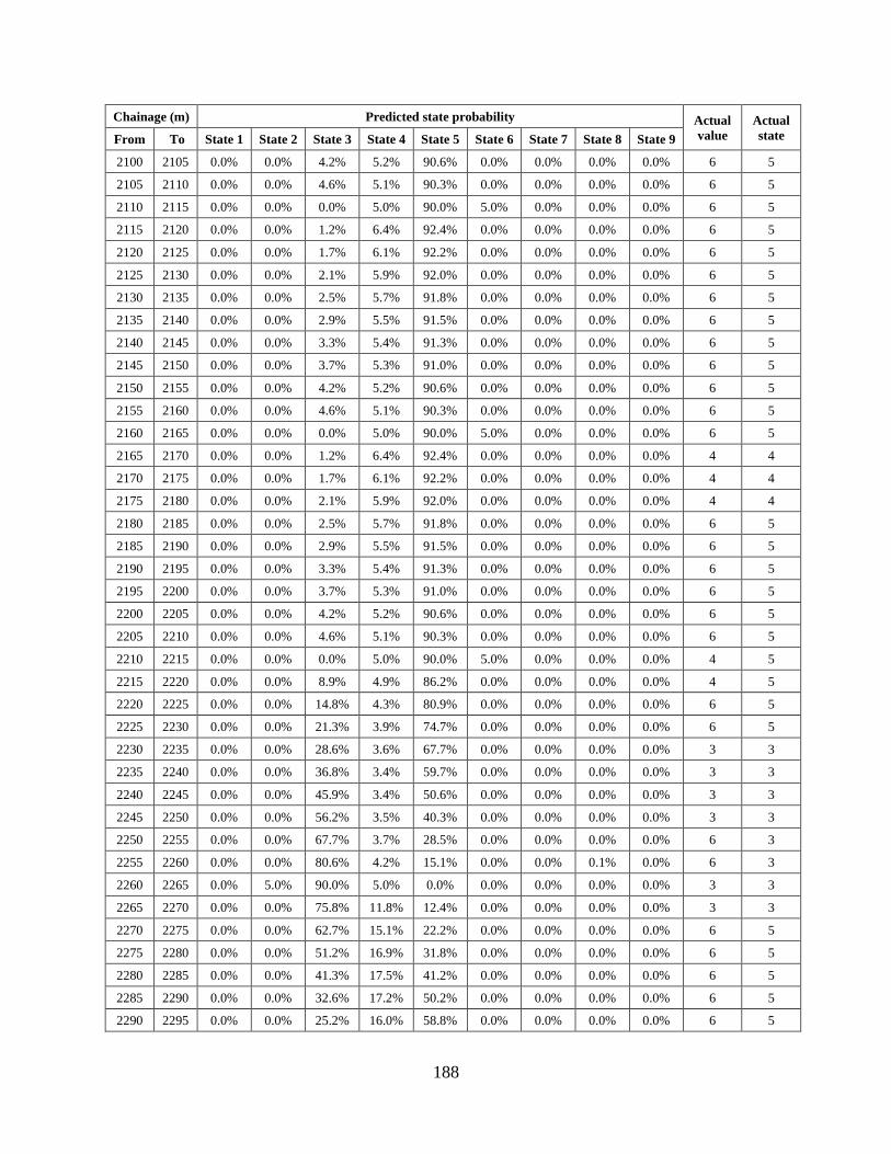
188
Chainage (m) Predicted state probability Actual
value
Actual
state From To State 1 State 2 State 3 State 4 State 5 State 6 State 7 State 8 State 9
2100 2105 0.0% 0.0% 4.2% 5.2% 90.6% 0.0% 0.0% 0.0% 0.0% 6 5
2105 2110 0.0% 0.0% 4.6% 5.1% 90.3% 0.0% 0.0% 0.0% 0.0% 6 5
2110 2115 0.0% 0.0% 0.0% 5.0% 90.0% 5.0% 0.0% 0.0% 0.0% 6 5
2115 2120 0.0% 0.0% 1.2% 6.4% 92.4% 0.0% 0.0% 0.0% 0.0% 6 5
2120 2125 0.0% 0.0% 1.7% 6.1% 92.2% 0.0% 0.0% 0.0% 0.0% 6 5
2125 2130 0.0% 0.0% 2.1% 5.9% 92.0% 0.0% 0.0% 0.0% 0.0% 6 5
2130 2135 0.0% 0.0% 2.5% 5.7% 91.8% 0.0% 0.0% 0.0% 0.0% 6 5
2135 2140 0.0% 0.0% 2.9% 5.5% 91.5% 0.0% 0.0% 0.0% 0.0% 6 5
2140 2145 0.0% 0.0% 3.3% 5.4% 91.3% 0.0% 0.0% 0.0% 0.0% 6 5
2145 2150 0.0% 0.0% 3.7% 5.3% 91.0% 0.0% 0.0% 0.0% 0.0% 6 5
2150 2155 0.0% 0.0% 4.2% 5.2% 90.6% 0.0% 0.0% 0.0% 0.0% 6 5
2155 2160 0.0% 0.0% 4.6% 5.1% 90.3% 0.0% 0.0% 0.0% 0.0% 6 5
2160 2165 0.0% 0.0% 0.0% 5.0% 90.0% 5.0% 0.0% 0.0% 0.0% 6 5
2165 2170 0.0% 0.0% 1.2% 6.4% 92.4% 0.0% 0.0% 0.0% 0.0% 4 4
2170 2175 0.0% 0.0% 1.7% 6.1% 92.2% 0.0% 0.0% 0.0% 0.0% 4 4
2175 2180 0.0% 0.0% 2.1% 5.9% 92.0% 0.0% 0.0% 0.0% 0.0% 4 4
2180 2185 0.0% 0.0% 2.5% 5.7% 91.8% 0.0% 0.0% 0.0% 0.0% 6 5
2185 2190 0.0% 0.0% 2.9% 5.5% 91.5% 0.0% 0.0% 0.0% 0.0% 6 5
2190 2195 0.0% 0.0% 3.3% 5.4% 91.3% 0.0% 0.0% 0.0% 0.0% 6 5
2195 2200 0.0% 0.0% 3.7% 5.3% 91.0% 0.0% 0.0% 0.0% 0.0% 6 5
2200 2205 0.0% 0.0% 4.2% 5.2% 90.6% 0.0% 0.0% 0.0% 0.0% 6 5
2205 2210 0.0% 0.0% 4.6% 5.1% 90.3% 0.0% 0.0% 0.0% 0.0% 6 5
2210 2215 0.0% 0.0% 0.0% 5.0% 90.0% 5.0% 0.0% 0.0% 0.0% 4 5
2215 2220 0.0% 0.0% 8.9% 4.9% 86.2% 0.0% 0.0% 0.0% 0.0% 4 5
2220 2225 0.0% 0.0% 14.8% 4.3% 80.9% 0.0% 0.0% 0.0% 0.0% 6 5
2225 2230 0.0% 0.0% 21.3% 3.9% 74.7% 0.0% 0.0% 0.0% 0.0% 6 5
2230 2235 0.0% 0.0% 28.6% 3.6% 67.7% 0.0% 0.0% 0.0% 0.0% 3 3
2235 2240 0.0% 0.0% 36.8% 3.4% 59.7% 0.0% 0.0% 0.0% 0.0% 3 3
2240 2245 0.0% 0.0% 45.9% 3.4% 50.6% 0.0% 0.0% 0.0% 0.0% 3 3
2245 2250 0.0% 0.0% 56.2% 3.5% 40.3% 0.0% 0.0% 0.0% 0.0% 3 3
2250 2255 0.0% 0.0% 67.7% 3.7% 28.5% 0.0% 0.0% 0.0% 0.0% 6 3
2255 2260 0.0% 0.0% 80.6% 4.2% 15.1% 0.0% 0.0% 0.1% 0.0% 6 3
2260 2265 0.0% 5.0% 90.0% 5.0% 0.0% 0.0% 0.0% 0.0% 0.0% 3 3
2265 2270 0.0% 0.0% 75.8% 11.8% 12.4% 0.0% 0.0% 0.0% 0.0% 3 3
2270 2275 0.0% 0.0% 62.7% 15.1% 22.2% 0.0% 0.0% 0.0% 0.0% 6 5
2275 2280 0.0% 0.0% 51.2% 16.9% 31.8% 0.0% 0.0% 0.0% 0.0% 6 5
2280 2285 0.0% 0.0% 41.3% 17.5% 41.2% 0.0% 0.0% 0.0% 0.0% 6 5
2285 2290 0.0% 0.0% 32.6% 17.2% 50.2% 0.0% 0.0% 0.0% 0.0% 6 5
2290 2295 0.0% 0.0% 25.2% 16.0% 58.8% 0.0% 0.0% 0.0% 0.0% 6 5
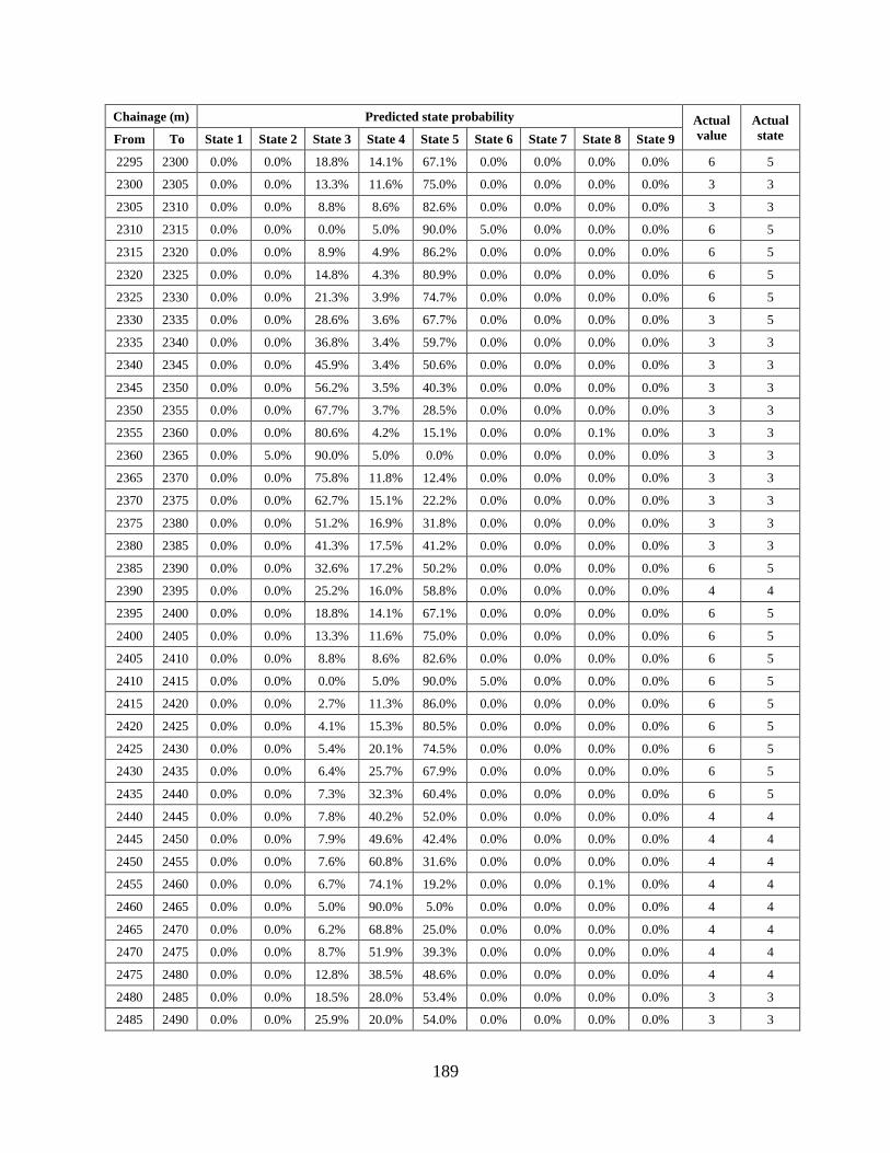
189
Chainage (m) Predicted state probability Actual
value
Actual
state From To State 1 State 2 State 3 State 4 State 5 State 6 State 7 State 8 State 9
2295 2300 0.0% 0.0% 18.8% 14.1% 67.1% 0.0% 0.0% 0.0% 0.0% 6 5
2300 2305 0.0% 0.0% 13.3% 11.6% 75.0% 0.0% 0.0% 0.0% 0.0% 3 3
2305 2310 0.0% 0.0% 8.8% 8.6% 82.6% 0.0% 0.0% 0.0% 0.0% 3 3
2310 2315 0.0% 0.0% 0.0% 5.0% 90.0% 5.0% 0.0% 0.0% 0.0% 6 5
2315 2320 0.0% 0.0% 8.9% 4.9% 86.2% 0.0% 0.0% 0.0% 0.0% 6 5
2320 2325 0.0% 0.0% 14.8% 4.3% 80.9% 0.0% 0.0% 0.0% 0.0% 6 5
2325 2330 0.0% 0.0% 21.3% 3.9% 74.7% 0.0% 0.0% 0.0% 0.0% 6 5
2330 2335 0.0% 0.0% 28.6% 3.6% 67.7% 0.0% 0.0% 0.0% 0.0% 3 5
2335 2340 0.0% 0.0% 36.8% 3.4% 59.7% 0.0% 0.0% 0.0% 0.0% 3 3
2340 2345 0.0% 0.0% 45.9% 3.4% 50.6% 0.0% 0.0% 0.0% 0.0% 3 3
2345 2350 0.0% 0.0% 56.2% 3.5% 40.3% 0.0% 0.0% 0.0% 0.0% 3 3
2350 2355 0.0% 0.0% 67.7% 3.7% 28.5% 0.0% 0.0% 0.0% 0.0% 3 3
2355 2360 0.0% 0.0% 80.6% 4.2% 15.1% 0.0% 0.0% 0.1% 0.0% 3 3
2360 2365 0.0% 5.0% 90.0% 5.0% 0.0% 0.0% 0.0% 0.0% 0.0% 3 3
2365 2370 0.0% 0.0% 75.8% 11.8% 12.4% 0.0% 0.0% 0.0% 0.0% 3 3
2370 2375 0.0% 0.0% 62.7% 15.1% 22.2% 0.0% 0.0% 0.0% 0.0% 3 3
2375 2380 0.0% 0.0% 51.2% 16.9% 31.8% 0.0% 0.0% 0.0% 0.0% 3 3
2380 2385 0.0% 0.0% 41.3% 17.5% 41.2% 0.0% 0.0% 0.0% 0.0% 3 3
2385 2390 0.0% 0.0% 32.6% 17.2% 50.2% 0.0% 0.0% 0.0% 0.0% 6 5
2390 2395 0.0% 0.0% 25.2% 16.0% 58.8% 0.0% 0.0% 0.0% 0.0% 4 4
2395 2400 0.0% 0.0% 18.8% 14.1% 67.1% 0.0% 0.0% 0.0% 0.0% 6 5
2400 2405 0.0% 0.0% 13.3% 11.6% 75.0% 0.0% 0.0% 0.0% 0.0% 6 5
2405 2410 0.0% 0.0% 8.8% 8.6% 82.6% 0.0% 0.0% 0.0% 0.0% 6 5
2410 2415 0.0% 0.0% 0.0% 5.0% 90.0% 5.0% 0.0% 0.0% 0.0% 6 5
2415 2420 0.0% 0.0% 2.7% 11.3% 86.0% 0.0% 0.0% 0.0% 0.0% 6 5
2420 2425 0.0% 0.0% 4.1% 15.3% 80.5% 0.0% 0.0% 0.0% 0.0% 6 5
2425 2430 0.0% 0.0% 5.4% 20.1% 74.5% 0.0% 0.0% 0.0% 0.0% 6 5
2430 2435 0.0% 0.0% 6.4% 25.7% 67.9% 0.0% 0.0% 0.0% 0.0% 6 5
2435 2440 0.0% 0.0% 7.3% 32.3% 60.4% 0.0% 0.0% 0.0% 0.0% 6 5
2440 2445 0.0% 0.0% 7.8% 40.2% 52.0% 0.0% 0.0% 0.0% 0.0% 4 4
2445 2450 0.0% 0.0% 7.9% 49.6% 42.4% 0.0% 0.0% 0.0% 0.0% 4 4
2450 2455 0.0% 0.0% 7.6% 60.8% 31.6% 0.0% 0.0% 0.0% 0.0% 4 4
2455 2460 0.0% 0.0% 6.7% 74.1% 19.2% 0.0% 0.0% 0.1% 0.0% 4 4
2460 2465 0.0% 0.0% 5.0% 90.0% 5.0% 0.0% 0.0% 0.0% 0.0% 4 4
2465 2470 0.0% 0.0% 6.2% 68.8% 25.0% 0.0% 0.0% 0.0% 0.0% 4 4
2470 2475 0.0% 0.0% 8.7% 51.9% 39.3% 0.0% 0.0% 0.0% 0.0% 4 4
2475 2480 0.0% 0.0% 12.8% 38.5% 48.6% 0.0% 0.0% 0.0% 0.0% 4 4
2480 2485 0.0% 0.0% 18.5% 28.0% 53.4% 0.0% 0.0% 0.0% 0.0% 3 3
2485 2490 0.0% 0.0% 25.9% 20.0% 54.0% 0.0% 0.0% 0.0% 0.0% 3 3

190
Chainage (m) Predicted state probability Actual
value
Actual
state From To State 1 State 2 State 3 State 4 State 5 State 6 State 7 State 8 State 9
2490 2495 0.0% 0.0% 35.2% 14.1% 50.7% 0.0% 0.0% 0.0% 0.0% 3 3
2495 2500 0.0% 0.0% 46.6% 9.8% 43.6% 0.0% 0.0% 0.0% 0.0% 3 3
2500 2505 0.0% 0.0% 60.2% 7.0% 32.8% 0.0% 0.0% 0.1% 0.0% 3 3
2505 2510 0.0% 0.0% 76.3% 5.4% 18.2% 0.0% 0.0% 0.1% 0.0% 3 3
2510 2515 0.0% 5.0% 90.0% 5.0% 0.0% 0.0% 0.0% 0.0% 0.0% 3 3
2515 2520 0.0% 0.0% 92.6% 4.8% 2.6% 0.0% 0.0% 0.0% 0.0% 3 3
2520 2525 0.0% 0.0% 91.8% 4.3% 3.9% 0.0% 0.0% 0.0% 0.0% 3 3
2525 2530 0.0% 0.0% 91.3% 3.9% 4.7% 0.0% 0.0% 0.0% 0.0% 3 3
2530 2535 0.0% 0.0% 91.1% 3.7% 5.3% 0.0% 0.0% 0.0% 0.0% 3 3
2535 2540 0.0% 0.0% 91.1% 3.5% 5.4% 0.0% 0.0% 0.0% 0.0% 3 3
2540 2545 0.0% 0.0% 91.3% 3.6% 5.1% 0.0% 0.0% 0.0% 0.0% 3 3
2545 2550 0.0% 0.0% 91.8% 3.7% 4.5% 0.0% 0.0% 0.0% 0.0% 3 3
2550 2555 0.0% 0.0% 92.6% 4.0% 3.4% 0.0% 0.0% 0.0% 0.0% 3 3
2555 2560 0.0% 0.0% 93.6% 4.4% 1.9% 0.0% 0.0% 0.0% 0.0% 3 3
2560 2565 0.0% 5.0% 90.0% 5.0% 0.0% 0.0% 0.0% 0.0% 0.0% 3 3
2565 2570 0.0% 0.0% 92.6% 4.8% 2.6% 0.0% 0.0% 0.0% 0.0% 3 3
2570 2575 0.0% 0.0% 91.8% 4.3% 3.9% 0.0% 0.0% 0.0% 0.0% 3 3
2575 2580 0.0% 0.0% 91.3% 3.9% 4.7% 0.0% 0.0% 0.0% 0.0% 3 3
2580 2585 0.0% 0.0% 91.1% 3.7% 5.3% 0.0% 0.0% 0.0% 0.0% 3 3
2585 2590 0.0% 0.0% 91.1% 3.5% 5.4% 0.0% 0.0% 0.0% 0.0% 3 3
2590 2595 0.0% 0.0% 91.3% 3.6% 5.1% 0.0% 0.0% 0.0% 0.0% 3 3
2595 2600 0.0% 0.0% 91.8% 3.7% 4.5% 0.0% 0.0% 0.0% 0.0% 3 3
2600 2605 0.0% 0.0% 92.6% 4.0% 3.4% 0.0% 0.0% 0.0% 0.0% 3 3
2605 2610 0.0% 0.0% 93.6% 4.4% 1.9% 0.0% 0.0% 0.0% 0.0% 3 3
2610 2615 0.0% 5.0% 90.0% 5.0% 0.0% 0.0% 0.0% 0.0% 0.0% 3 3
Table F.4 Comparison between predicted and actual Jr in Subsection 2
Chainage (m) Predicted state probability Actual
value
Actual
state From To State 1 State 2 State 3 State 4 State 5 State 6 State 7
2010 2015 0.0% 5.0% 5.0% 85.0% 5.0% 0.0% 0.0% 1.5 4
2015 2020 0.4% 0.0% 0.0% 91.3% 8.3% 0.0% 0.0% 1.5 4
2020 2025 0.8% 0.0% 0.0% 92.5% 6.7% 0.0% 0.0% 1.5 4
2025 2030 1.1% 0.0% 0.0% 93.1% 5.8% 0.0% 0.0% 1.5 4
2030 2035 1.4% 0.0% 0.0% 93.3% 5.2% 0.0% 0.0% 1.5 4
2035 2040 1.8% 0.0% 0.0% 93.2% 5.0% 0.0% 0.0% 1.5 4
2040 2045 2.3% 0.0% 0.0% 92.6% 5.1% 0.0% 0.0% 1.5 4
2045 2050 2.8% 0.0% 0.0% 91.6% 5.6% 0.0% 0.0% 1.5 4
2050 2055 3.4% 0.0% 0.0% 90.1% 6.5% 0.0% 0.0% 1.5 4
2055 2060 4.2% 0.0% 0.0% 87.9% 7.9% 0.0% 0.0% 1.5 4
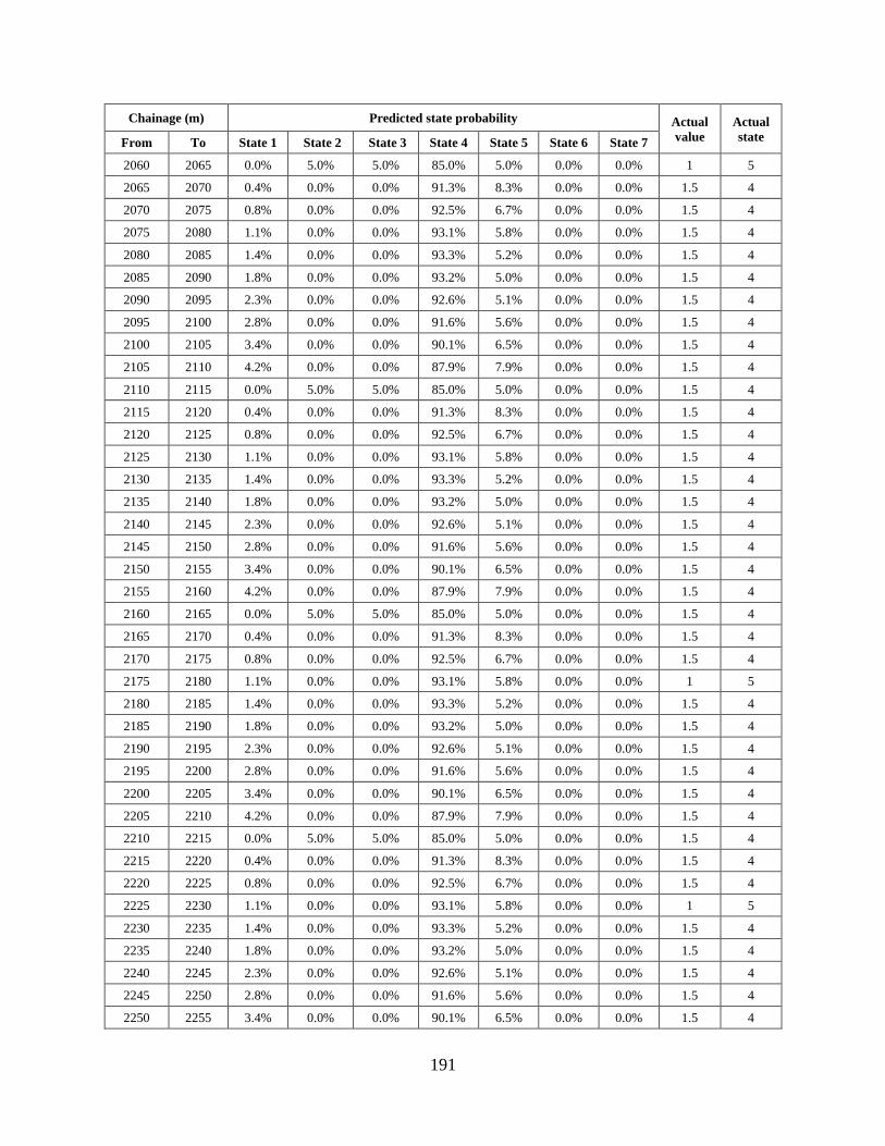
191
Chainage (m) Predicted state probability Actual
value
Actual
state From To State 1 State 2 State 3 State 4 State 5 State 6 State 7
2060 2065 0.0% 5.0% 5.0% 85.0% 5.0% 0.0% 0.0% 1 5
2065 2070 0.4% 0.0% 0.0% 91.3% 8.3% 0.0% 0.0% 1.5 4
2070 2075 0.8% 0.0% 0.0% 92.5% 6.7% 0.0% 0.0% 1.5 4
2075 2080 1.1% 0.0% 0.0% 93.1% 5.8% 0.0% 0.0% 1.5 4
2080 2085 1.4% 0.0% 0.0% 93.3% 5.2% 0.0% 0.0% 1.5 4
2085 2090 1.8% 0.0% 0.0% 93.2% 5.0% 0.0% 0.0% 1.5 4
2090 2095 2.3% 0.0% 0.0% 92.6% 5.1% 0.0% 0.0% 1.5 4
2095 2100 2.8% 0.0% 0.0% 91.6% 5.6% 0.0% 0.0% 1.5 4
2100 2105 3.4% 0.0% 0.0% 90.1% 6.5% 0.0% 0.0% 1.5 4
2105 2110 4.2% 0.0% 0.0% 87.9% 7.9% 0.0% 0.0% 1.5 4
2110 2115 0.0% 5.0% 5.0% 85.0% 5.0% 0.0% 0.0% 1.5 4
2115 2120 0.4% 0.0% 0.0% 91.3% 8.3% 0.0% 0.0% 1.5 4
2120 2125 0.8% 0.0% 0.0% 92.5% 6.7% 0.0% 0.0% 1.5 4
2125 2130 1.1% 0.0% 0.0% 93.1% 5.8% 0.0% 0.0% 1.5 4
2130 2135 1.4% 0.0% 0.0% 93.3% 5.2% 0.0% 0.0% 1.5 4
2135 2140 1.8% 0.0% 0.0% 93.2% 5.0% 0.0% 0.0% 1.5 4
2140 2145 2.3% 0.0% 0.0% 92.6% 5.1% 0.0% 0.0% 1.5 4
2145 2150 2.8% 0.0% 0.0% 91.6% 5.6% 0.0% 0.0% 1.5 4
2150 2155 3.4% 0.0% 0.0% 90.1% 6.5% 0.0% 0.0% 1.5 4
2155 2160 4.2% 0.0% 0.0% 87.9% 7.9% 0.0% 0.0% 1.5 4
2160 2165 0.0% 5.0% 5.0% 85.0% 5.0% 0.0% 0.0% 1.5 4
2165 2170 0.4% 0.0% 0.0% 91.3% 8.3% 0.0% 0.0% 1.5 4
2170 2175 0.8% 0.0% 0.0% 92.5% 6.7% 0.0% 0.0% 1.5 4
2175 2180 1.1% 0.0% 0.0% 93.1% 5.8% 0.0% 0.0% 1 5
2180 2185 1.4% 0.0% 0.0% 93.3% 5.2% 0.0% 0.0% 1.5 4
2185 2190 1.8% 0.0% 0.0% 93.2% 5.0% 0.0% 0.0% 1.5 4
2190 2195 2.3% 0.0% 0.0% 92.6% 5.1% 0.0% 0.0% 1.5 4
2195 2200 2.8% 0.0% 0.0% 91.6% 5.6% 0.0% 0.0% 1.5 4
2200 2205 3.4% 0.0% 0.0% 90.1% 6.5% 0.0% 0.0% 1.5 4
2205 2210 4.2% 0.0% 0.0% 87.9% 7.9% 0.0% 0.0% 1.5 4
2210 2215 0.0% 5.0% 5.0% 85.0% 5.0% 0.0% 0.0% 1.5 4
2215 2220 0.4% 0.0% 0.0% 91.3% 8.3% 0.0% 0.0% 1.5 4
2220 2225 0.8% 0.0% 0.0% 92.5% 6.7% 0.0% 0.0% 1.5 4
2225 2230 1.1% 0.0% 0.0% 93.1% 5.8% 0.0% 0.0% 1 5
2230 2235 1.4% 0.0% 0.0% 93.3% 5.2% 0.0% 0.0% 1.5 4
2235 2240 1.8% 0.0% 0.0% 93.2% 5.0% 0.0% 0.0% 1.5 4
2240 2245 2.3% 0.0% 0.0% 92.6% 5.1% 0.0% 0.0% 1.5 4
2245 2250 2.8% 0.0% 0.0% 91.6% 5.6% 0.0% 0.0% 1.5 4
2250 2255 3.4% 0.0% 0.0% 90.1% 6.5% 0.0% 0.0% 1.5 4
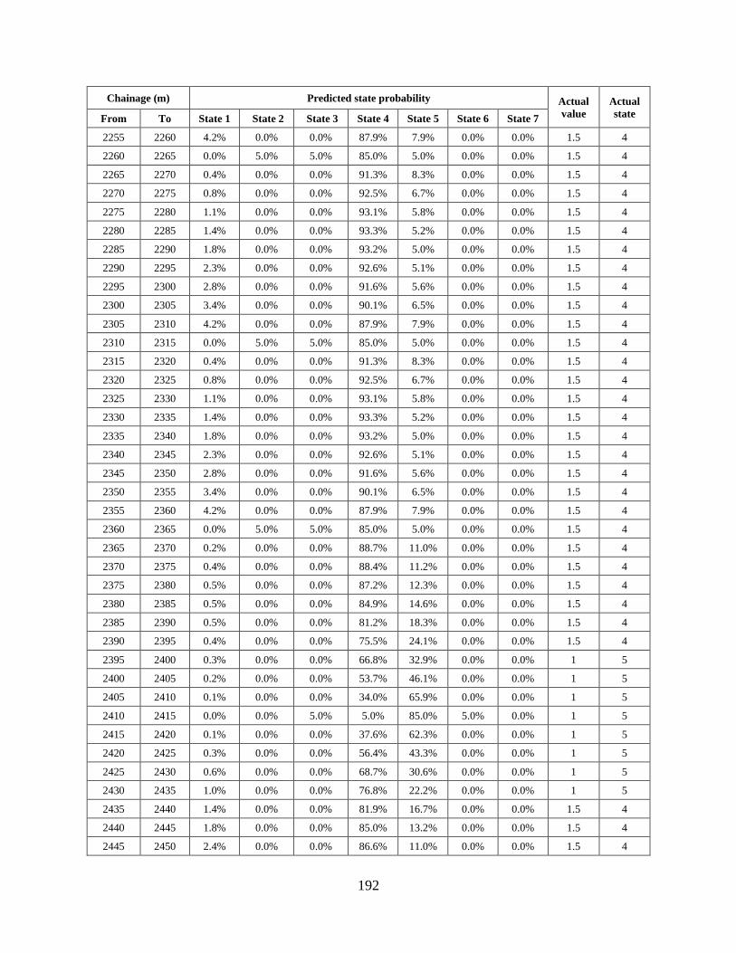
192
Chainage (m) Predicted state probability Actual
value
Actual
state From To State 1 State 2 State 3 State 4 State 5 State 6 State 7
2255 2260 4.2% 0.0% 0.0% 87.9% 7.9% 0.0% 0.0% 1.5 4
2260 2265 0.0% 5.0% 5.0% 85.0% 5.0% 0.0% 0.0% 1.5 4
2265 2270 0.4% 0.0% 0.0% 91.3% 8.3% 0.0% 0.0% 1.5 4
2270 2275 0.8% 0.0% 0.0% 92.5% 6.7% 0.0% 0.0% 1.5 4
2275 2280 1.1% 0.0% 0.0% 93.1% 5.8% 0.0% 0.0% 1.5 4
2280 2285 1.4% 0.0% 0.0% 93.3% 5.2% 0.0% 0.0% 1.5 4
2285 2290 1.8% 0.0% 0.0% 93.2% 5.0% 0.0% 0.0% 1.5 4
2290 2295 2.3% 0.0% 0.0% 92.6% 5.1% 0.0% 0.0% 1.5 4
2295 2300 2.8% 0.0% 0.0% 91.6% 5.6% 0.0% 0.0% 1.5 4
2300 2305 3.4% 0.0% 0.0% 90.1% 6.5% 0.0% 0.0% 1.5 4
2305 2310 4.2% 0.0% 0.0% 87.9% 7.9% 0.0% 0.0% 1.5 4
2310 2315 0.0% 5.0% 5.0% 85.0% 5.0% 0.0% 0.0% 1.5 4
2315 2320 0.4% 0.0% 0.0% 91.3% 8.3% 0.0% 0.0% 1.5 4
2320 2325 0.8% 0.0% 0.0% 92.5% 6.7% 0.0% 0.0% 1.5 4
2325 2330 1.1% 0.0% 0.0% 93.1% 5.8% 0.0% 0.0% 1.5 4
2330 2335 1.4% 0.0% 0.0% 93.3% 5.2% 0.0% 0.0% 1.5 4
2335 2340 1.8% 0.0% 0.0% 93.2% 5.0% 0.0% 0.0% 1.5 4
2340 2345 2.3% 0.0% 0.0% 92.6% 5.1% 0.0% 0.0% 1.5 4
2345 2350 2.8% 0.0% 0.0% 91.6% 5.6% 0.0% 0.0% 1.5 4
2350 2355 3.4% 0.0% 0.0% 90.1% 6.5% 0.0% 0.0% 1.5 4
2355 2360 4.2% 0.0% 0.0% 87.9% 7.9% 0.0% 0.0% 1.5 4
2360 2365 0.0% 5.0% 5.0% 85.0% 5.0% 0.0% 0.0% 1.5 4
2365 2370 0.2% 0.0% 0.0% 88.7% 11.0% 0.0% 0.0% 1.5 4
2370 2375 0.4% 0.0% 0.0% 88.4% 11.2% 0.0% 0.0% 1.5 4
2375 2380 0.5% 0.0% 0.0% 87.2% 12.3% 0.0% 0.0% 1.5 4
2380 2385 0.5% 0.0% 0.0% 84.9% 14.6% 0.0% 0.0% 1.5 4
2385 2390 0.5% 0.0% 0.0% 81.2% 18.3% 0.0% 0.0% 1.5 4
2390 2395 0.4% 0.0% 0.0% 75.5% 24.1% 0.0% 0.0% 1.5 4
2395 2400 0.3% 0.0% 0.0% 66.8% 32.9% 0.0% 0.0% 1 5
2400 2405 0.2% 0.0% 0.0% 53.7% 46.1% 0.0% 0.0% 1 5
2405 2410 0.1% 0.0% 0.0% 34.0% 65.9% 0.0% 0.0% 1 5
2410 2415 0.0% 0.0% 5.0% 5.0% 85.0% 5.0% 0.0% 1 5
2415 2420 0.1% 0.0% 0.0% 37.6% 62.3% 0.0% 0.0% 1 5
2420 2425 0.3% 0.0% 0.0% 56.4% 43.3% 0.0% 0.0% 1 5
2425 2430 0.6% 0.0% 0.0% 68.7% 30.6% 0.0% 0.0% 1 5
2430 2435 1.0% 0.0% 0.0% 76.8% 22.2% 0.0% 0.0% 1 5
2435 2440 1.4% 0.0% 0.0% 81.9% 16.7% 0.0% 0.0% 1.5 4
2440 2445 1.8% 0.0% 0.0% 85.0% 13.2% 0.0% 0.0% 1.5 4
2445 2450 2.4% 0.0% 0.0% 86.6% 11.0% 0.0% 0.0% 1.5 4
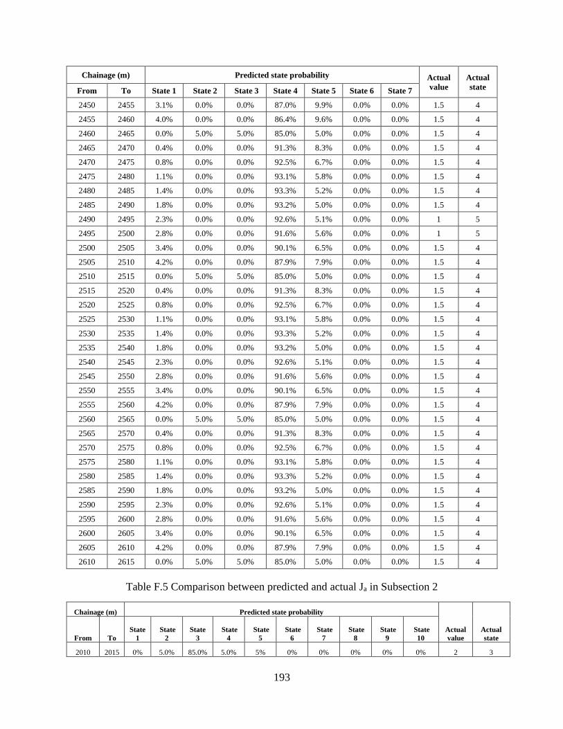
193
Chainage (m) Predicted state probability Actual
value
Actual
state From To State 1 State 2 State 3 State 4 State 5 State 6 State 7
2450 2455 3.1% 0.0% 0.0% 87.0% 9.9% 0.0% 0.0% 1.5 4
2455 2460 4.0% 0.0% 0.0% 86.4% 9.6% 0.0% 0.0% 1.5 4
2460 2465 0.0% 5.0% 5.0% 85.0% 5.0% 0.0% 0.0% 1.5 4
2465 2470 0.4% 0.0% 0.0% 91.3% 8.3% 0.0% 0.0% 1.5 4
2470 2475 0.8% 0.0% 0.0% 92.5% 6.7% 0.0% 0.0% 1.5 4
2475 2480 1.1% 0.0% 0.0% 93.1% 5.8% 0.0% 0.0% 1.5 4
2480 2485 1.4% 0.0% 0.0% 93.3% 5.2% 0.0% 0.0% 1.5 4
2485 2490 1.8% 0.0% 0.0% 93.2% 5.0% 0.0% 0.0% 1.5 4
2490 2495 2.3% 0.0% 0.0% 92.6% 5.1% 0.0% 0.0% 1 5
2495 2500 2.8% 0.0% 0.0% 91.6% 5.6% 0.0% 0.0% 1 5
2500 2505 3.4% 0.0% 0.0% 90.1% 6.5% 0.0% 0.0% 1.5 4
2505 2510 4.2% 0.0% 0.0% 87.9% 7.9% 0.0% 0.0% 1.5 4
2510 2515 0.0% 5.0% 5.0% 85.0% 5.0% 0.0% 0.0% 1.5 4
2515 2520 0.4% 0.0% 0.0% 91.3% 8.3% 0.0% 0.0% 1.5 4
2520 2525 0.8% 0.0% 0.0% 92.5% 6.7% 0.0% 0.0% 1.5 4
2525 2530 1.1% 0.0% 0.0% 93.1% 5.8% 0.0% 0.0% 1.5 4
2530 2535 1.4% 0.0% 0.0% 93.3% 5.2% 0.0% 0.0% 1.5 4
2535 2540 1.8% 0.0% 0.0% 93.2% 5.0% 0.0% 0.0% 1.5 4
2540 2545 2.3% 0.0% 0.0% 92.6% 5.1% 0.0% 0.0% 1.5 4
2545 2550 2.8% 0.0% 0.0% 91.6% 5.6% 0.0% 0.0% 1.5 4
2550 2555 3.4% 0.0% 0.0% 90.1% 6.5% 0.0% 0.0% 1.5 4
2555 2560 4.2% 0.0% 0.0% 87.9% 7.9% 0.0% 0.0% 1.5 4
2560 2565 0.0% 5.0% 5.0% 85.0% 5.0% 0.0% 0.0% 1.5 4
2565 2570 0.4% 0.0% 0.0% 91.3% 8.3% 0.0% 0.0% 1.5 4
2570 2575 0.8% 0.0% 0.0% 92.5% 6.7% 0.0% 0.0% 1.5 4
2575 2580 1.1% 0.0% 0.0% 93.1% 5.8% 0.0% 0.0% 1.5 4
2580 2585 1.4% 0.0% 0.0% 93.3% 5.2% 0.0% 0.0% 1.5 4
2585 2590 1.8% 0.0% 0.0% 93.2% 5.0% 0.0% 0.0% 1.5 4
2590 2595 2.3% 0.0% 0.0% 92.6% 5.1% 0.0% 0.0% 1.5 4
2595 2600 2.8% 0.0% 0.0% 91.6% 5.6% 0.0% 0.0% 1.5 4
2600 2605 3.4% 0.0% 0.0% 90.1% 6.5% 0.0% 0.0% 1.5 4
2605 2610 4.2% 0.0% 0.0% 87.9% 7.9% 0.0% 0.0% 1.5 4
2610 2615 0.0% 5.0% 5.0% 85.0% 5.0% 0.0% 0.0% 1.5 4
Table F.5 Comparison between predicted and actual Ja in Subsection 2
Chainage (m) Predicted state probability
Actual
value
Actual
state From To
State
1
State
2
State
3
State
4
State
5
State
6
State
7
State
8
State
9
State
10
2010 2015 0% 5.0% 85.0% 5.0% 5% 0% 0% 0% 0% 0% 2 3
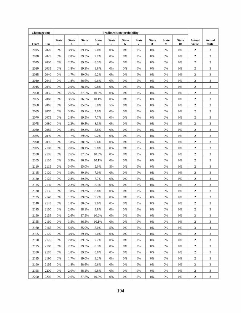
194
Chainage (m) Predicted state probability
Actual
value
Actual
state From To
State
1
State
2
State
3
State
4
State
5
State
6
State
7
State
8
State
9
State
10
2015 2020 0% 3.9% 89.1% 7.0% 0% 0% 0% 0% 0% 0% 2 3
2020 2025 0% 2.8% 89.5% 7.7% 0% 0% 0% 0% 0% 0% 2 3
2025 2030 0% 2.2% 89.5% 8.3% 0% 0% 0% 0% 0% 0% 2 3
2030 2035 0% 1.8% 89.3% 8.8% 0% 0% 0% 0% 0% 0% 2 3
2035 2040 0% 1.7% 89.0% 9.2% 0% 0% 0% 0% 0% 0% 2 3
2040 2045 0% 1.8% 88.6% 9.6% 0% 0% 0% 0% 0% 0% 2 3
2045 2050 0% 2.0% 88.1% 9.8% 0% 0% 0% 0% 0% 0% 2 3
2050 2055 0% 2.6% 87.5% 10.0% 0% 0% 0% 0% 0% 0% 2 3
2055 2060 0% 3.5% 86.5% 10.1% 0% 0% 0% 0% 0% 0% 2 3
2060 2065 0% 5.0% 85.0% 5.0% 5% 0% 0% 0% 0% 0% 2 3
2065 2070 0% 3.9% 89.1% 7.0% 0% 0% 0% 0% 0% 0% 2 3
2070 2075 0% 2.8% 89.5% 7.7% 0% 0% 0% 0% 0% 0% 2 3
2075 2080 0% 2.2% 89.5% 8.3% 0% 0% 0% 0% 0% 0% 2 3
2080 2085 0% 1.8% 89.3% 8.8% 0% 0% 0% 0% 0% 0% 2 3
2085 2090 0% 1.7% 89.0% 9.2% 0% 0% 0% 0% 0% 0% 2 3
2090 2095 0% 1.8% 88.6% 9.6% 0% 0% 0% 0% 0% 0% 2 3
2095 2100 0% 2.0% 88.1% 9.8% 0% 0% 0% 0% 0% 0% 2 3
2100 2105 0% 2.6% 87.5% 10.0% 0% 0% 0% 0% 0% 0% 2 3
2105 2110 0% 3.5% 86.5% 10.1% 0% 0% 0% 0% 0% 0% 2 3
2110 2115 0% 5.0% 85.0% 5.0% 5% 0% 0% 0% 0% 0% 2 3
2115 2120 0% 3.9% 89.1% 7.0% 0% 0% 0% 0% 0% 0% 2 3
2120 2125 0% 2.8% 89.5% 7.7% 0% 0% 0% 0% 0% 0% 2 3
2125 2130 0% 2.2% 89.5% 8.3% 0% 0% 0% 0% 0% 0% 2 3
2130 2135 0% 1.8% 89.3% 8.8% 0% 0% 0% 0% 0% 0% 2 3
2135 2140 0% 1.7% 89.0% 9.2% 0% 0% 0% 0% 0% 0% 2 3
2140 2145 0% 1.8% 88.6% 9.6% 0% 0% 0% 0% 0% 0% 2 3
2145 2150 0% 2.0% 88.1% 9.8% 0% 0% 0% 0% 0% 0% 2 3
2150 2155 0% 2.6% 87.5% 10.0% 0% 0% 0% 0% 0% 0% 2 3
2155 2160 0% 3.5% 86.5% 10.1% 0% 0% 0% 0% 0% 0% 2 3
2160 2165 0% 5.0% 85.0% 5.0% 5% 0% 0% 0% 0% 0% 3 4
2165 2170 0% 3.9% 89.1% 7.0% 0% 0% 0% 0% 0% 0% 2 3
2170 2175 0% 2.8% 89.5% 7.7% 0% 0% 0% 0% 0% 0% 2 3
2175 2180 0% 2.2% 89.5% 8.3% 0% 0% 0% 0% 0% 0% 2 3
2180 2185 0% 1.8% 89.3% 8.8% 0% 0% 0% 0% 0% 0% 2 3
2185 2190 0% 1.7% 89.0% 9.2% 0% 0% 0% 0% 0% 0% 2 3
2190 2195 0% 1.8% 88.6% 9.6% 0% 0% 0% 0% 0% 0% 2 3
2195 2200 0% 2.0% 88.1% 9.8% 0% 0% 0% 0% 0% 0% 2 3
2200 2205 0% 2.6% 87.5% 10.0% 0% 0% 0% 0% 0% 0% 2 3
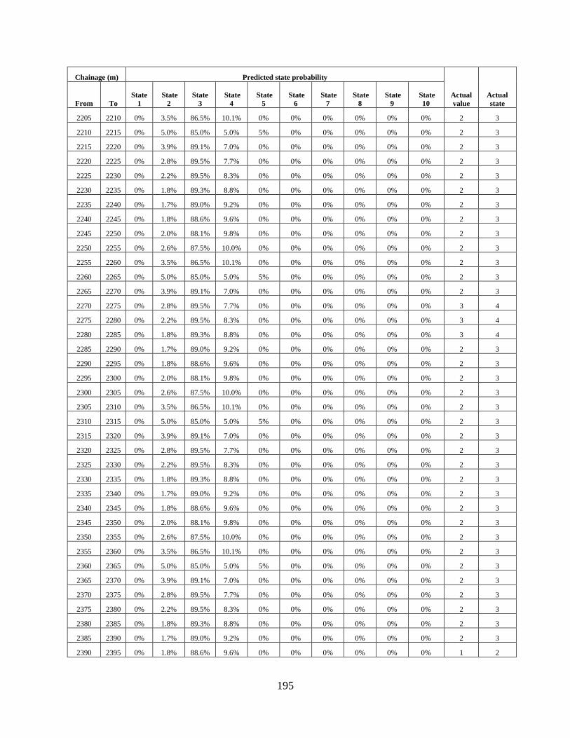
195
Chainage (m) Predicted state probability
Actual
value
Actual
state From To
State
1
State
2
State
3
State
4
State
5
State
6
State
7
State
8
State
9
State
10
2205 2210 0% 3.5% 86.5% 10.1% 0% 0% 0% 0% 0% 0% 2 3
2210 2215 0% 5.0% 85.0% 5.0% 5% 0% 0% 0% 0% 0% 2 3
2215 2220 0% 3.9% 89.1% 7.0% 0% 0% 0% 0% 0% 0% 2 3
2220 2225 0% 2.8% 89.5% 7.7% 0% 0% 0% 0% 0% 0% 2 3
2225 2230 0% 2.2% 89.5% 8.3% 0% 0% 0% 0% 0% 0% 2 3
2230 2235 0% 1.8% 89.3% 8.8% 0% 0% 0% 0% 0% 0% 2 3
2235 2240 0% 1.7% 89.0% 9.2% 0% 0% 0% 0% 0% 0% 2 3
2240 2245 0% 1.8% 88.6% 9.6% 0% 0% 0% 0% 0% 0% 2 3
2245 2250 0% 2.0% 88.1% 9.8% 0% 0% 0% 0% 0% 0% 2 3
2250 2255 0% 2.6% 87.5% 10.0% 0% 0% 0% 0% 0% 0% 2 3
2255 2260 0% 3.5% 86.5% 10.1% 0% 0% 0% 0% 0% 0% 2 3
2260 2265 0% 5.0% 85.0% 5.0% 5% 0% 0% 0% 0% 0% 2 3
2265 2270 0% 3.9% 89.1% 7.0% 0% 0% 0% 0% 0% 0% 2 3
2270 2275 0% 2.8% 89.5% 7.7% 0% 0% 0% 0% 0% 0% 3 4
2275 2280 0% 2.2% 89.5% 8.3% 0% 0% 0% 0% 0% 0% 3 4
2280 2285 0% 1.8% 89.3% 8.8% 0% 0% 0% 0% 0% 0% 3 4
2285 2290 0% 1.7% 89.0% 9.2% 0% 0% 0% 0% 0% 0% 2 3
2290 2295 0% 1.8% 88.6% 9.6% 0% 0% 0% 0% 0% 0% 2 3
2295 2300 0% 2.0% 88.1% 9.8% 0% 0% 0% 0% 0% 0% 2 3
2300 2305 0% 2.6% 87.5% 10.0% 0% 0% 0% 0% 0% 0% 2 3
2305 2310 0% 3.5% 86.5% 10.1% 0% 0% 0% 0% 0% 0% 2 3
2310 2315 0% 5.0% 85.0% 5.0% 5% 0% 0% 0% 0% 0% 2 3
2315 2320 0% 3.9% 89.1% 7.0% 0% 0% 0% 0% 0% 0% 2 3
2320 2325 0% 2.8% 89.5% 7.7% 0% 0% 0% 0% 0% 0% 2 3
2325 2330 0% 2.2% 89.5% 8.3% 0% 0% 0% 0% 0% 0% 2 3
2330 2335 0% 1.8% 89.3% 8.8% 0% 0% 0% 0% 0% 0% 2 3
2335 2340 0% 1.7% 89.0% 9.2% 0% 0% 0% 0% 0% 0% 2 3
2340 2345 0% 1.8% 88.6% 9.6% 0% 0% 0% 0% 0% 0% 2 3
2345 2350 0% 2.0% 88.1% 9.8% 0% 0% 0% 0% 0% 0% 2 3
2350 2355 0% 2.6% 87.5% 10.0% 0% 0% 0% 0% 0% 0% 2 3
2355 2360 0% 3.5% 86.5% 10.1% 0% 0% 0% 0% 0% 0% 2 3
2360 2365 0% 5.0% 85.0% 5.0% 5% 0% 0% 0% 0% 0% 2 3
2365 2370 0% 3.9% 89.1% 7.0% 0% 0% 0% 0% 0% 0% 2 3
2370 2375 0% 2.8% 89.5% 7.7% 0% 0% 0% 0% 0% 0% 2 3
2375 2380 0% 2.2% 89.5% 8.3% 0% 0% 0% 0% 0% 0% 2 3
2380 2385 0% 1.8% 89.3% 8.8% 0% 0% 0% 0% 0% 0% 2 3
2385 2390 0% 1.7% 89.0% 9.2% 0% 0% 0% 0% 0% 0% 2 3
2390 2395 0% 1.8% 88.6% 9.6% 0% 0% 0% 0% 0% 0% 1 2
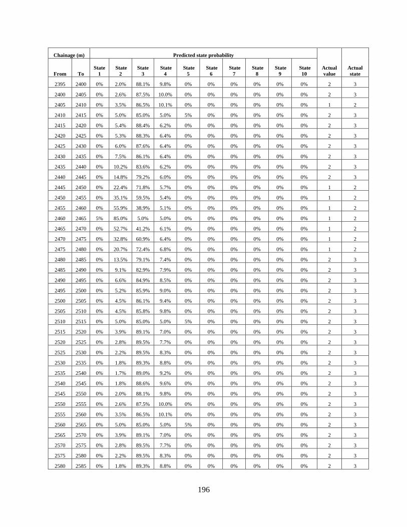
196
Chainage (m) Predicted state probability
Actual
value
Actual
state From To
State
1
State
2
State
3
State
4
State
5
State
6
State
7
State
8
State
9
State
10
2395 2400 0% 2.0% 88.1% 9.8% 0% 0% 0% 0% 0% 0% 2 3
2400 2405 0% 2.6% 87.5% 10.0% 0% 0% 0% 0% 0% 0% 2 3
2405 2410 0% 3.5% 86.5% 10.1% 0% 0% 0% 0% 0% 0% 1 2
2410 2415 0% 5.0% 85.0% 5.0% 5% 0% 0% 0% 0% 0% 2 3
2415 2420 0% 5.4% 88.4% 6.2% 0% 0% 0% 0% 0% 0% 2 3
2420 2425 0% 5.3% 88.3% 6.4% 0% 0% 0% 0% 0% 0% 2 3
2425 2430 0% 6.0% 87.6% 6.4% 0% 0% 0% 0% 0% 0% 2 3
2430 2435 0% 7.5% 86.1% 6.4% 0% 0% 0% 0% 0% 0% 2 3
2435 2440 0% 10.2% 83.6% 6.2% 0% 0% 0% 0% 0% 0% 2 3
2440 2445 0% 14.8% 79.2% 6.0% 0% 0% 0% 0% 0% 0% 2 3
2445 2450 0% 22.4% 71.8% 5.7% 0% 0% 0% 0% 0% 0% 1 2
2450 2455 0% 35.1% 59.5% 5.4% 0% 0% 0% 0% 0% 0% 1 2
2455 2460 0% 55.9% 38.9% 5.1% 0% 0% 0% 0% 0% 0% 1 2
2460 2465 5% 85.0% 5.0% 5.0% 0% 0% 0% 0% 0% 0% 1 2
2465 2470 0% 52.7% 41.2% 6.1% 0% 0% 0% 0% 0% 0% 1 2
2470 2475 0% 32.8% 60.9% 6.4% 0% 0% 0% 0% 0% 0% 1 2
2475 2480 0% 20.7% 72.4% 6.8% 0% 0% 0% 0% 0% 0% 1 2
2480 2485 0% 13.5% 79.1% 7.4% 0% 0% 0% 0% 0% 0% 2 3
2485 2490 0% 9.1% 82.9% 7.9% 0% 0% 0% 0% 0% 0% 2 3
2490 2495 0% 6.6% 84.9% 8.5% 0% 0% 0% 0% 0% 0% 2 3
2495 2500 0% 5.2% 85.9% 9.0% 0% 0% 0% 0% 0% 0% 2 3
2500 2505 0% 4.5% 86.1% 9.4% 0% 0% 0% 0% 0% 0% 2 3
2505 2510 0% 4.5% 85.8% 9.8% 0% 0% 0% 0% 0% 0% 2 3
2510 2515 0% 5.0% 85.0% 5.0% 5% 0% 0% 0% 0% 0% 2 3
2515 2520 0% 3.9% 89.1% 7.0% 0% 0% 0% 0% 0% 0% 2 3
2520 2525 0% 2.8% 89.5% 7.7% 0% 0% 0% 0% 0% 0% 2 3
2525 2530 0% 2.2% 89.5% 8.3% 0% 0% 0% 0% 0% 0% 2 3
2530 2535 0% 1.8% 89.3% 8.8% 0% 0% 0% 0% 0% 0% 2 3
2535 2540 0% 1.7% 89.0% 9.2% 0% 0% 0% 0% 0% 0% 2 3
2540 2545 0% 1.8% 88.6% 9.6% 0% 0% 0% 0% 0% 0% 2 3
2545 2550 0% 2.0% 88.1% 9.8% 0% 0% 0% 0% 0% 0% 2 3
2550 2555 0% 2.6% 87.5% 10.0% 0% 0% 0% 0% 0% 0% 2 3
2555 2560 0% 3.5% 86.5% 10.1% 0% 0% 0% 0% 0% 0% 2 3
2560 2565 0% 5.0% 85.0% 5.0% 5% 0% 0% 0% 0% 0% 2 3
2565 2570 0% 3.9% 89.1% 7.0% 0% 0% 0% 0% 0% 0% 2 3
2570 2575 0% 2.8% 89.5% 7.7% 0% 0% 0% 0% 0% 0% 2 3
2575 2580 0% 2.2% 89.5% 8.3% 0% 0% 0% 0% 0% 0% 2 3
2580 2585 0% 1.8% 89.3% 8.8% 0% 0% 0% 0% 0% 0% 2 3

197
Chainage (m) Predicted state probability
Actual
value
Actual
state From To
State
1
State
2
State
3
State
4
State
5
State
6
State
7
State
8
State
9
State
10
2585 2590 0% 1.7% 89.0% 9.2% 0% 0% 0% 0% 0% 0% 2 3
2590 2595 0% 1.8% 88.6% 9.6% 0% 0% 0% 0% 0% 0% 2 3
2595 2600 0% 2.0% 88.1% 9.8% 0% 0% 0% 0% 0% 0% 2 3
2600 2605 0% 2.6% 87.5% 10.0% 0% 0% 0% 0% 0% 0% 2 3
2605 2610 0% 3.5% 86.5% 10.1% 0% 0% 0% 0% 0% 0% 2 3
2610 2615 0% 5.0% 85.0% 5.0% 5% 0% 0% 0% 0% 0% 2 3
Table F.6 Comparison between predicted and actual Jw in Subsection 2
Chainage (m) Predicted state probability Actual
value
Actual
state From To State 1 State 2 State 3 State 4 State 5 State 6
2010 2015 95% 5% 0% 0% 0% 0% 1 1
2015 2020 95% 5% 0% 0% 0% 0% 1 1
2020 2025 95% 5% 0% 0% 0% 0% 1 1
2025 2030 94% 6% 0% 0% 0% 0% 1 1
2030 2035 94% 6% 0% 0% 0% 0% 1 1
2035 2040 94% 6% 0% 0% 0% 0% 1 1
2040 2045 94% 6% 0% 0% 0% 0% 1 1
2045 2050 94% 6% 0% 0% 0% 0% 1 1
2050 2055 95% 5% 0% 0% 0% 0% 1 1
2055 2060 95% 5% 0% 0% 0% 0% 1 1
2060 2065 95% 5% 0% 0% 0% 0% 1 1
2065 2070 95% 5% 0% 0% 0% 0% 1 1
2070 2075 95% 5% 0% 0% 0% 0% 1 1
2075 2080 94% 6% 0% 0% 0% 0% 1 1
2080 2085 94% 6% 0% 0% 0% 0% 1 1
2085 2090 94% 6% 0% 0% 0% 0% 1 1
2090 2095 94% 6% 0% 0% 0% 0% 1 1
2095 2100 94% 6% 0% 0% 0% 0% 1 1
2100 2105 95% 5% 0% 0% 0% 0% 1 1
2105 2110 95% 5% 0% 0% 0% 0% 1 1
2110 2115 95% 5% 0% 0% 0% 0% 1 1
2115 2120 95% 5% 0% 0% 0% 0% 1 1
2120 2125 95% 5% 0% 0% 0% 0% 1 1
2125 2130 94% 6% 0% 0% 0% 0% 1 1
2130 2135 94% 6% 0% 0% 0% 0% 1 1
2135 2140 94% 6% 0% 0% 0% 0% 1 1
2140 2145 94% 6% 0% 0% 0% 0% 1 1
2145 2150 94% 6% 0% 0% 0% 0% 1 1
2150 2155 95% 5% 0% 0% 0% 0% 1 1
2155 2160 95% 5% 0% 0% 0% 0% 1 1
2160 2165 95% 5% 0% 0% 0% 0% 1 1
2165 2170 95% 5% 0% 0% 0% 0% 1 1
2170 2175 95% 5% 0% 0% 0% 0% 0.66 2
2175 2180 94% 6% 0% 0% 0% 0% 0.5 3
2180 2185 94% 6% 0% 0% 0% 0% 0.66 2
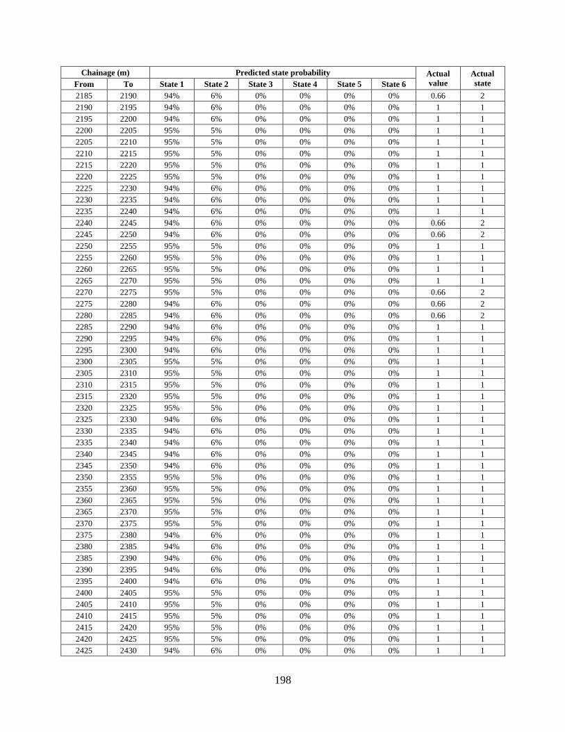
198
Chainage (m) Predicted state probability Actual
value
Actual
state From To State 1 State 2 State 3 State 4 State 5 State 6
2185 2190 94% 6% 0% 0% 0% 0% 0.66 2
2190 2195 94% 6% 0% 0% 0% 0% 1 1
2195 2200 94% 6% 0% 0% 0% 0% 1 1
2200 2205 95% 5% 0% 0% 0% 0% 1 1
2205 2210 95% 5% 0% 0% 0% 0% 1 1
2210 2215 95% 5% 0% 0% 0% 0% 1 1
2215 2220 95% 5% 0% 0% 0% 0% 1 1
2220 2225 95% 5% 0% 0% 0% 0% 1 1
2225 2230 94% 6% 0% 0% 0% 0% 1 1
2230 2235 94% 6% 0% 0% 0% 0% 1 1
2235 2240 94% 6% 0% 0% 0% 0% 1 1
2240 2245 94% 6% 0% 0% 0% 0% 0.66 2
2245 2250 94% 6% 0% 0% 0% 0% 0.66 2
2250 2255 95% 5% 0% 0% 0% 0% 1 1
2255 2260 95% 5% 0% 0% 0% 0% 1 1
2260 2265 95% 5% 0% 0% 0% 0% 1 1
2265 2270 95% 5% 0% 0% 0% 0% 1 1
2270 2275 95% 5% 0% 0% 0% 0% 0.66 2
2275 2280 94% 6% 0% 0% 0% 0% 0.66 2
2280 2285 94% 6% 0% 0% 0% 0% 0.66 2
2285 2290 94% 6% 0% 0% 0% 0% 1 1
2290 2295 94% 6% 0% 0% 0% 0% 1 1
2295 2300 94% 6% 0% 0% 0% 0% 1 1
2300 2305 95% 5% 0% 0% 0% 0% 1 1
2305 2310 95% 5% 0% 0% 0% 0% 1 1
2310 2315 95% 5% 0% 0% 0% 0% 1 1
2315 2320 95% 5% 0% 0% 0% 0% 1 1
2320 2325 95% 5% 0% 0% 0% 0% 1 1
2325 2330 94% 6% 0% 0% 0% 0% 1 1
2330 2335 94% 6% 0% 0% 0% 0% 1 1
2335 2340 94% 6% 0% 0% 0% 0% 1 1
2340 2345 94% 6% 0% 0% 0% 0% 1 1
2345 2350 94% 6% 0% 0% 0% 0% 1 1
2350 2355 95% 5% 0% 0% 0% 0% 1 1
2355 2360 95% 5% 0% 0% 0% 0% 1 1
2360 2365 95% 5% 0% 0% 0% 0% 1 1
2365 2370 95% 5% 0% 0% 0% 0% 1 1
2370 2375 95% 5% 0% 0% 0% 0% 1 1
2375 2380 94% 6% 0% 0% 0% 0% 1 1
2380 2385 94% 6% 0% 0% 0% 0% 1 1
2385 2390 94% 6% 0% 0% 0% 0% 1 1
2390 2395 94% 6% 0% 0% 0% 0% 1 1
2395 2400 94% 6% 0% 0% 0% 0% 1 1
2400 2405 95% 5% 0% 0% 0% 0% 1 1
2405 2410 95% 5% 0% 0% 0% 0% 1 1
2410 2415 95% 5% 0% 0% 0% 0% 1 1
2415 2420 95% 5% 0% 0% 0% 0% 1 1
2420 2425 95% 5% 0% 0% 0% 0% 1 1
2425 2430 94% 6% 0% 0% 0% 0% 1 1
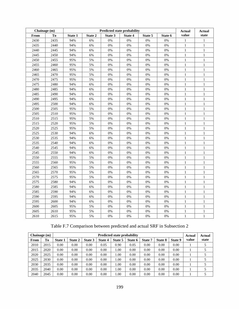
199
Chainage (m) Predicted state probability Actual
value
Actual
state From To State 1 State 2 State 3 State 4 State 5 State 6
2430 2435 94% 6% 0% 0% 0% 0% 1 1
2435 2440 94% 6% 0% 0% 0% 0% 1 1
2440 2445 94% 6% 0% 0% 0% 0% 1 1
2445 2450 94% 6% 0% 0% 0% 0% 1 1
2450 2455 95% 5% 0% 0% 0% 0% 1 1
2455 2460 95% 5% 0% 0% 0% 0% 1 1
2460 2465 95% 5% 0% 0% 0% 0% 1 1
2465 2470 95% 5% 0% 0% 0% 0% 1 1
2470 2475 95% 5% 0% 0% 0% 0% 1 1
2475 2480 94% 6% 0% 0% 0% 0% 1 1
2480 2485 94% 6% 0% 0% 0% 0% 1 1
2485 2490 94% 6% 0% 0% 0% 0% 1 1
2490 2495 94% 6% 0% 0% 0% 0% 1 1
2495 2500 94% 6% 0% 0% 0% 0% 1 1
2500 2505 95% 5% 0% 0% 0% 0% 1 1
2505 2510 95% 5% 0% 0% 0% 0% 1 1
2510 2515 95% 5% 0% 0% 0% 0% 1 1
2515 2520 95% 5% 0% 0% 0% 0% 1 1
2520 2525 95% 5% 0% 0% 0% 0% 1 1
2525 2530 94% 6% 0% 0% 0% 0% 1 1
2530 2535 94% 6% 0% 0% 0% 0% 1 1
2535 2540 94% 6% 0% 0% 0% 0% 1 1
2540 2545 94% 6% 0% 0% 0% 0% 1 1
2545 2550 94% 6% 0% 0% 0% 0% 1 1
2550 2555 95% 5% 0% 0% 0% 0% 1 1
2555 2560 95% 5% 0% 0% 0% 0% 1 1
2560 2565 95% 5% 0% 0% 0% 0% 1 1
2565 2570 95% 5% 0% 0% 0% 0% 1 1
2570 2575 95% 5% 0% 0% 0% 0% 1 1
2575 2580 94% 6% 0% 0% 0% 0% 1 1
2580 2585 94% 6% 0% 0% 0% 0% 1 1
2585 2590 94% 6% 0% 0% 0% 0% 1 1
2590 2595 94% 6% 0% 0% 0% 0% 1 1
2595 2600 94% 6% 0% 0% 0% 0% 1 1
2600 2605 95% 5% 0% 0% 0% 0% 1 1
2605 2610 95% 5% 0% 0% 0% 0% 1 1
2610 2615 95% 5% 0% 0% 0% 0% 1 1
Table F.7 Comparison between predicted and actual SRF in Subsection 2
Chainage (m) Predicted state probability Actual
value
Actual
state From To State 1 State 2 State 3 State 4 State 5 State 6 State 7 State 8 State 9
2010 2015 0.00 0.00 0.00 0.05 0.90 0.05 0.00 0.00 0.00 1 5
2015 2020 0.00 0.00 0.00 0.00 1.00 0.00 0.00 0.00 0.00 1 5
2020 2025 0.00 0.00 0.00 0.00 1.00 0.00 0.00 0.00 0.00 1 5
2025 2030 0.00 0.00 0.00 0.00 1.00 0.00 0.00 0.00 0.00 1 5
2030 2035 0.00 0.00 0.00 0.00 1.00 0.00 0.00 0.00 0.00 1 5
2035 2040 0.00 0.00 0.00 0.00 1.00 0.00 0.00 0.00 0.00 1 5
2040 2045 0.00 0.00 0.00 0.00 1.00 0.00 0.00 0.00 0.00 1 5
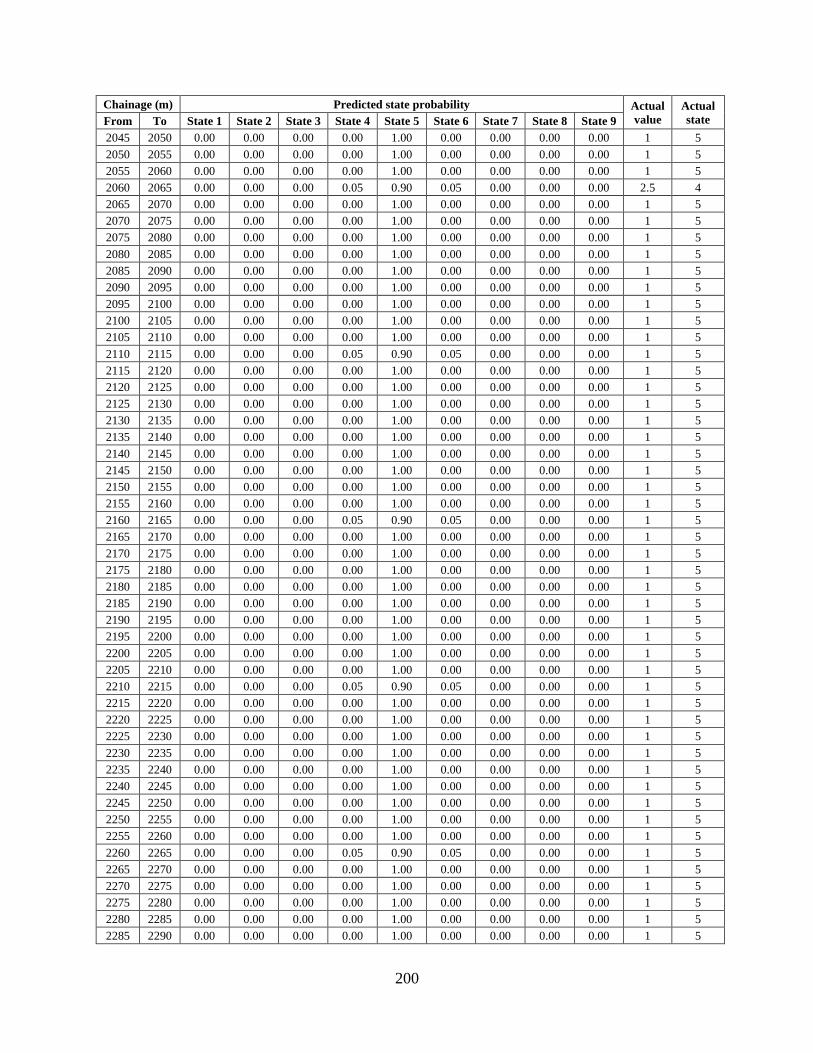
200
Chainage (m) Predicted state probability Actual
value
Actual
state From To State 1 State 2 State 3 State 4 State 5 State 6 State 7 State 8 State 9
2045 2050 0.00 0.00 0.00 0.00 1.00 0.00 0.00 0.00 0.00 1 5
2050 2055 0.00 0.00 0.00 0.00 1.00 0.00 0.00 0.00 0.00 1 5
2055 2060 0.00 0.00 0.00 0.00 1.00 0.00 0.00 0.00 0.00 1 5
2060 2065 0.00 0.00 0.00 0.05 0.90 0.05 0.00 0.00 0.00 2.5 4
2065 2070 0.00 0.00 0.00 0.00 1.00 0.00 0.00 0.00 0.00 1 5
2070 2075 0.00 0.00 0.00 0.00 1.00 0.00 0.00 0.00 0.00 1 5
2075 2080 0.00 0.00 0.00 0.00 1.00 0.00 0.00 0.00 0.00 1 5
2080 2085 0.00 0.00 0.00 0.00 1.00 0.00 0.00 0.00 0.00 1 5
2085 2090 0.00 0.00 0.00 0.00 1.00 0.00 0.00 0.00 0.00 1 5
2090 2095 0.00 0.00 0.00 0.00 1.00 0.00 0.00 0.00 0.00 1 5
2095 2100 0.00 0.00 0.00 0.00 1.00 0.00 0.00 0.00 0.00 1 5
2100 2105 0.00 0.00 0.00 0.00 1.00 0.00 0.00 0.00 0.00 1 5
2105 2110 0.00 0.00 0.00 0.00 1.00 0.00 0.00 0.00 0.00 1 5
2110 2115 0.00 0.00 0.00 0.05 0.90 0.05 0.00 0.00 0.00 1 5
2115 2120 0.00 0.00 0.00 0.00 1.00 0.00 0.00 0.00 0.00 1 5
2120 2125 0.00 0.00 0.00 0.00 1.00 0.00 0.00 0.00 0.00 1 5
2125 2130 0.00 0.00 0.00 0.00 1.00 0.00 0.00 0.00 0.00 1 5
2130 2135 0.00 0.00 0.00 0.00 1.00 0.00 0.00 0.00 0.00 1 5
2135 2140 0.00 0.00 0.00 0.00 1.00 0.00 0.00 0.00 0.00 1 5
2140 2145 0.00 0.00 0.00 0.00 1.00 0.00 0.00 0.00 0.00 1 5
2145 2150 0.00 0.00 0.00 0.00 1.00 0.00 0.00 0.00 0.00 1 5
2150 2155 0.00 0.00 0.00 0.00 1.00 0.00 0.00 0.00 0.00 1 5
2155 2160 0.00 0.00 0.00 0.00 1.00 0.00 0.00 0.00 0.00 1 5
2160 2165 0.00 0.00 0.00 0.05 0.90 0.05 0.00 0.00 0.00 1 5
2165 2170 0.00 0.00 0.00 0.00 1.00 0.00 0.00 0.00 0.00 1 5
2170 2175 0.00 0.00 0.00 0.00 1.00 0.00 0.00 0.00 0.00 1 5
2175 2180 0.00 0.00 0.00 0.00 1.00 0.00 0.00 0.00 0.00 1 5
2180 2185 0.00 0.00 0.00 0.00 1.00 0.00 0.00 0.00 0.00 1 5
2185 2190 0.00 0.00 0.00 0.00 1.00 0.00 0.00 0.00 0.00 1 5
2190 2195 0.00 0.00 0.00 0.00 1.00 0.00 0.00 0.00 0.00 1 5
2195 2200 0.00 0.00 0.00 0.00 1.00 0.00 0.00 0.00 0.00 1 5
2200 2205 0.00 0.00 0.00 0.00 1.00 0.00 0.00 0.00 0.00 1 5
2205 2210 0.00 0.00 0.00 0.00 1.00 0.00 0.00 0.00 0.00 1 5
2210 2215 0.00 0.00 0.00 0.05 0.90 0.05 0.00 0.00 0.00 1 5
2215 2220 0.00 0.00 0.00 0.00 1.00 0.00 0.00 0.00 0.00 1 5
2220 2225 0.00 0.00 0.00 0.00 1.00 0.00 0.00 0.00 0.00 1 5
2225 2230 0.00 0.00 0.00 0.00 1.00 0.00 0.00 0.00 0.00 1 5
2230 2235 0.00 0.00 0.00 0.00 1.00 0.00 0.00 0.00 0.00 1 5
2235 2240 0.00 0.00 0.00 0.00 1.00 0.00 0.00 0.00 0.00 1 5
2240 2245 0.00 0.00 0.00 0.00 1.00 0.00 0.00 0.00 0.00 1 5
2245 2250 0.00 0.00 0.00 0.00 1.00 0.00 0.00 0.00 0.00 1 5
2250 2255 0.00 0.00 0.00 0.00 1.00 0.00 0.00 0.00 0.00 1 5
2255 2260 0.00 0.00 0.00 0.00 1.00 0.00 0.00 0.00 0.00 1 5
2260 2265 0.00 0.00 0.00 0.05 0.90 0.05 0.00 0.00 0.00 1 5
2265 2270 0.00 0.00 0.00 0.00 1.00 0.00 0.00 0.00 0.00 1 5
2270 2275 0.00 0.00 0.00 0.00 1.00 0.00 0.00 0.00 0.00 1 5
2275 2280 0.00 0.00 0.00 0.00 1.00 0.00 0.00 0.00 0.00 1 5
2280 2285 0.00 0.00 0.00 0.00 1.00 0.00 0.00 0.00 0.00 1 5
2285 2290 0.00 0.00 0.00 0.00 1.00 0.00 0.00 0.00 0.00 1 5
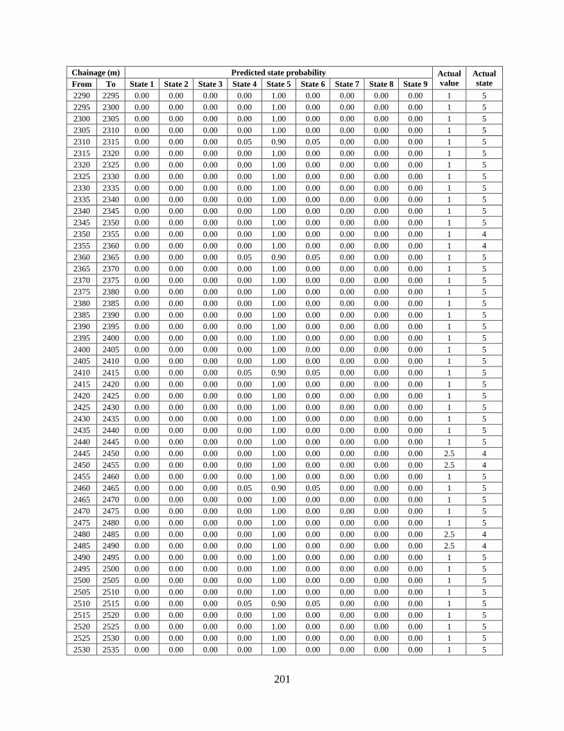
201
Chainage (m) Predicted state probability Actual
value
Actual
state From To State 1 State 2 State 3 State 4 State 5 State 6 State 7 State 8 State 9
2290 2295 0.00 0.00 0.00 0.00 1.00 0.00 0.00 0.00 0.00 1 5
2295 2300 0.00 0.00 0.00 0.00 1.00 0.00 0.00 0.00 0.00 1 5
2300 2305 0.00 0.00 0.00 0.00 1.00 0.00 0.00 0.00 0.00 1 5
2305 2310 0.00 0.00 0.00 0.00 1.00 0.00 0.00 0.00 0.00 1 5
2310 2315 0.00 0.00 0.00 0.05 0.90 0.05 0.00 0.00 0.00 1 5
2315 2320 0.00 0.00 0.00 0.00 1.00 0.00 0.00 0.00 0.00 1 5
2320 2325 0.00 0.00 0.00 0.00 1.00 0.00 0.00 0.00 0.00 1 5
2325 2330 0.00 0.00 0.00 0.00 1.00 0.00 0.00 0.00 0.00 1 5
2330 2335 0.00 0.00 0.00 0.00 1.00 0.00 0.00 0.00 0.00 1 5
2335 2340 0.00 0.00 0.00 0.00 1.00 0.00 0.00 0.00 0.00 1 5
2340 2345 0.00 0.00 0.00 0.00 1.00 0.00 0.00 0.00 0.00 1 5
2345 2350 0.00 0.00 0.00 0.00 1.00 0.00 0.00 0.00 0.00 1 5
2350 2355 0.00 0.00 0.00 0.00 1.00 0.00 0.00 0.00 0.00 1 4
2355 2360 0.00 0.00 0.00 0.00 1.00 0.00 0.00 0.00 0.00 1 4
2360 2365 0.00 0.00 0.00 0.05 0.90 0.05 0.00 0.00 0.00 1 5
2365 2370 0.00 0.00 0.00 0.00 1.00 0.00 0.00 0.00 0.00 1 5
2370 2375 0.00 0.00 0.00 0.00 1.00 0.00 0.00 0.00 0.00 1 5
2375 2380 0.00 0.00 0.00 0.00 1.00 0.00 0.00 0.00 0.00 1 5
2380 2385 0.00 0.00 0.00 0.00 1.00 0.00 0.00 0.00 0.00 1 5
2385 2390 0.00 0.00 0.00 0.00 1.00 0.00 0.00 0.00 0.00 1 5
2390 2395 0.00 0.00 0.00 0.00 1.00 0.00 0.00 0.00 0.00 1 5
2395 2400 0.00 0.00 0.00 0.00 1.00 0.00 0.00 0.00 0.00 1 5
2400 2405 0.00 0.00 0.00 0.00 1.00 0.00 0.00 0.00 0.00 1 5
2405 2410 0.00 0.00 0.00 0.00 1.00 0.00 0.00 0.00 0.00 1 5
2410 2415 0.00 0.00 0.00 0.05 0.90 0.05 0.00 0.00 0.00 1 5
2415 2420 0.00 0.00 0.00 0.00 1.00 0.00 0.00 0.00 0.00 1 5
2420 2425 0.00 0.00 0.00 0.00 1.00 0.00 0.00 0.00 0.00 1 5
2425 2430 0.00 0.00 0.00 0.00 1.00 0.00 0.00 0.00 0.00 1 5
2430 2435 0.00 0.00 0.00 0.00 1.00 0.00 0.00 0.00 0.00 1 5
2435 2440 0.00 0.00 0.00 0.00 1.00 0.00 0.00 0.00 0.00 1 5
2440 2445 0.00 0.00 0.00 0.00 1.00 0.00 0.00 0.00 0.00 1 5
2445 2450 0.00 0.00 0.00 0.00 1.00 0.00 0.00 0.00 0.00 2.5 4
2450 2455 0.00 0.00 0.00 0.00 1.00 0.00 0.00 0.00 0.00 2.5 4
2455 2460 0.00 0.00 0.00 0.00 1.00 0.00 0.00 0.00 0.00 1 5
2460 2465 0.00 0.00 0.00 0.05 0.90 0.05 0.00 0.00 0.00 1 5
2465 2470 0.00 0.00 0.00 0.00 1.00 0.00 0.00 0.00 0.00 1 5
2470 2475 0.00 0.00 0.00 0.00 1.00 0.00 0.00 0.00 0.00 1 5
2475 2480 0.00 0.00 0.00 0.00 1.00 0.00 0.00 0.00 0.00 1 5
2480 2485 0.00 0.00 0.00 0.00 1.00 0.00 0.00 0.00 0.00 2.5 4
2485 2490 0.00 0.00 0.00 0.00 1.00 0.00 0.00 0.00 0.00 2.5 4
2490 2495 0.00 0.00 0.00 0.00 1.00 0.00 0.00 0.00 0.00 1 5
2495 2500 0.00 0.00 0.00 0.00 1.00 0.00 0.00 0.00 0.00 1 5
2500 2505 0.00 0.00 0.00 0.00 1.00 0.00 0.00 0.00 0.00 1 5
2505 2510 0.00 0.00 0.00 0.00 1.00 0.00 0.00 0.00 0.00 1 5
2510 2515 0.00 0.00 0.00 0.05 0.90 0.05 0.00 0.00 0.00 1 5
2515 2520 0.00 0.00 0.00 0.00 1.00 0.00 0.00 0.00 0.00 1 5
2520 2525 0.00 0.00 0.00 0.00 1.00 0.00 0.00 0.00 0.00 1 5
2525 2530 0.00 0.00 0.00 0.00 1.00 0.00 0.00 0.00 0.00 1 5
2530 2535 0.00 0.00 0.00 0.00 1.00 0.00 0.00 0.00 0.00 1 5
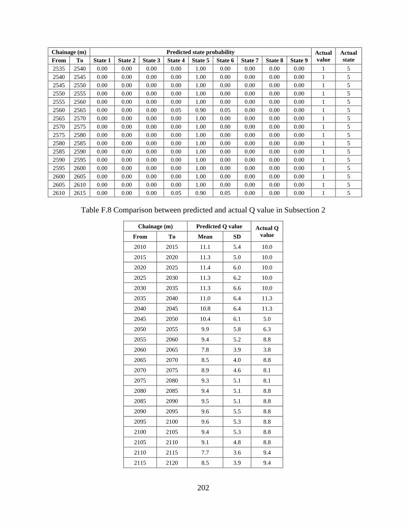
202
Chainage (m) Predicted state probability Actual
value
Actual
state From To State 1 State 2 State 3 State 4 State 5 State 6 State 7 State 8 State 9
2535 2540 0.00 0.00 0.00 0.00 1.00 0.00 0.00 0.00 0.00 1 5
2540 2545 0.00 0.00 0.00 0.00 1.00 0.00 0.00 0.00 0.00 1 5
2545 2550 0.00 0.00 0.00 0.00 1.00 0.00 0.00 0.00 0.00 1 5
2550 2555 0.00 0.00 0.00 0.00 1.00 0.00 0.00 0.00 0.00 1 5
2555 2560 0.00 0.00 0.00 0.00 1.00 0.00 0.00 0.00 0.00 1 5
2560 2565 0.00 0.00 0.00 0.05 0.90 0.05 0.00 0.00 0.00 1 5
2565 2570 0.00 0.00 0.00 0.00 1.00 0.00 0.00 0.00 0.00 1 5
2570 2575 0.00 0.00 0.00 0.00 1.00 0.00 0.00 0.00 0.00 1 5
2575 2580 0.00 0.00 0.00 0.00 1.00 0.00 0.00 0.00 0.00 1 5
2580 2585 0.00 0.00 0.00 0.00 1.00 0.00 0.00 0.00 0.00 1 5
2585 2590 0.00 0.00 0.00 0.00 1.00 0.00 0.00 0.00 0.00 1 5
2590 2595 0.00 0.00 0.00 0.00 1.00 0.00 0.00 0.00 0.00 1 5
2595 2600 0.00 0.00 0.00 0.00 1.00 0.00 0.00 0.00 0.00 1 5
2600 2605 0.00 0.00 0.00 0.00 1.00 0.00 0.00 0.00 0.00 1 5
2605 2610 0.00 0.00 0.00 0.00 1.00 0.00 0.00 0.00 0.00 1 5
2610 2615 0.00 0.00 0.00 0.05 0.90 0.05 0.00 0.00 0.00 1 5
Table F.8 Comparison between predicted and actual Q value in Subsection 2
Chainage (m) Predicted Q value Actual Q
value From To Mean SD
2010 2015 11.1 5.4 10.0
2015 2020 11.3 5.0 10.0
2020 2025 11.4 6.0 10.0
2025 2030 11.3 6.2 10.0
2030 2035 11.3 6.6 10.0
2035 2040 11.0 6.4 11.3
2040 2045 10.8 6.4 11.3
2045 2050 10.4 6.1 5.0
2050 2055 9.9 5.8 6.3
2055 2060 9.4 5.2 8.8
2060 2065 7.8 3.9 3.8
2065 2070 8.5 4.0 8.8
2070 2075 8.9 4.6 8.1
2075 2080 9.3 5.1 8.1
2080 2085 9.4 5.1 8.8
2085 2090 9.5 5.1 8.8
2090 2095 9.6 5.5 8.8
2095 2100 9.6 5.3 8.8
2100 2105 9.4 5.3 8.8
2105 2110 9.1 4.8 8.8
2110 2115 7.7 3.6 9.4
2115 2120 8.5 3.9 9.4
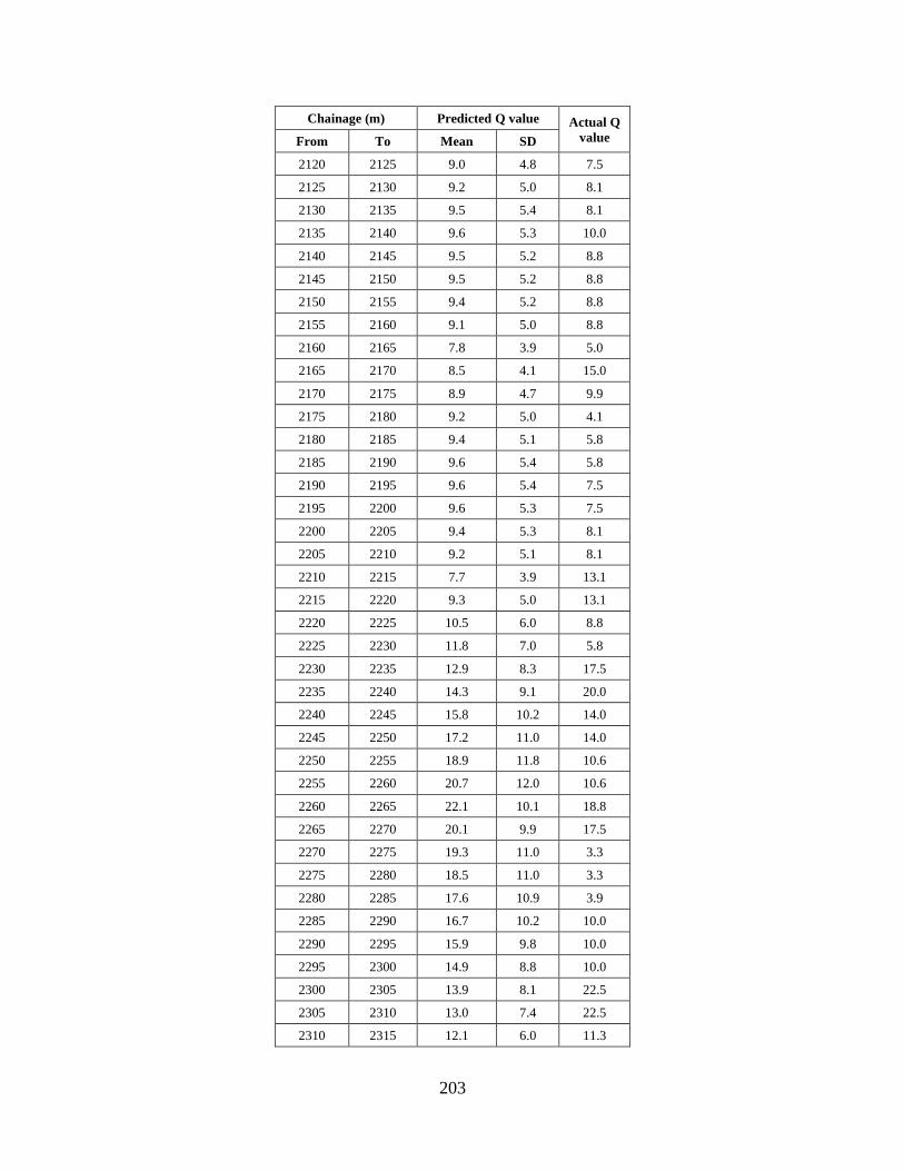
203
Chainage (m) Predicted Q value Actual Q
value From To Mean SD
2120 2125 9.0 4.8 7.5
2125 2130 9.2 5.0 8.1
2130 2135 9.5 5.4 8.1
2135 2140 9.6 5.3 10.0
2140 2145 9.5 5.2 8.8
2145 2150 9.5 5.2 8.8
2150 2155 9.4 5.2 8.8
2155 2160 9.1 5.0 8.8
2160 2165 7.8 3.9 5.0
2165 2170 8.5 4.1 15.0
2170 2175 8.9 4.7 9.9
2175 2180 9.2 5.0 4.1
2180 2185 9.4 5.1 5.8
2185 2190 9.6 5.4 5.8
2190 2195 9.6 5.4 7.5
2195 2200 9.6 5.3 7.5
2200 2205 9.4 5.3 8.1
2205 2210 9.2 5.1 8.1
2210 2215 7.7 3.9 13.1
2215 2220 9.3 5.0 13.1
2220 2225 10.5 6.0 8.8
2225 2230 11.8 7.0 5.8
2230 2235 12.9 8.3 17.5
2235 2240 14.3 9.1 20.0
2240 2245 15.8 10.2 14.0
2245 2250 17.2 11.0 14.0
2250 2255 18.9 11.8 10.6
2255 2260 20.7 12.0 10.6
2260 2265 22.1 10.1 18.8
2265 2270 20.1 9.9 17.5
2270 2275 19.3 11.0 3.3
2275 2280 18.5 11.0 3.3
2280 2285 17.6 10.9 3.9
2285 2290 16.7 10.2 10.0
2290 2295 15.9 9.8 10.0
2295 2300 14.9 8.8 10.0
2300 2305 13.9 8.1 22.5
2305 2310 13.0 7.4 22.5
2310 2315 12.1 6.0 11.3
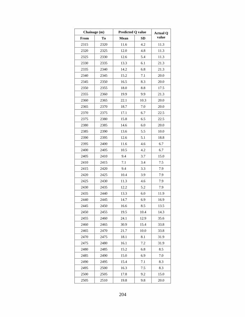
204
Chainage (m) Predicted Q value Actual Q
value From To Mean SD
2315 2320 11.6 4.2 11.3
2320 2325 12.0 4.8 11.3
2325 2330 12.6 5.4 11.3
2330 2335 13.3 6.1 21.3
2335 2340 14.2 6.8 21.3
2340 2345 15.2 7.1 20.0
2345 2350 16.5 8.3 20.0
2350 2355 18.0 8.8 17.5
2355 2360 19.9 9.9 21.3
2360 2365 22.1 10.3 20.0
2365 2370 18.7 7.0 20.0
2370 2375 17.1 6.7 22.5
2375 2380 15.8 6.5 22.5
2380 2385 14.6 6.0 20.0
2385 2390 13.6 5.5 10.0
2390 2395 12.6 5.1 18.8
2395 2400 11.6 4.6 6.7
2400 2405 10.5 4.2 6.7
2405 2410 9.4 3.7 15.0
2410 2415 7.1 3.4 7.5
2415 2420 9.4 3.3 7.9
2420 2425 10.4 3.9 7.9
2425 2430 11.3 4.6 7.9
2430 2435 12.2 5.2 7.9
2435 2440 13.3 6.0 11.9
2440 2445 14.7 6.9 16.9
2445 2450 16.6 8.5 13.5
2450 2455 19.5 10.4 14.3
2455 2460 24.1 12.9 35.6
2460 2465 30.9 15.4 33.8
2465 2470 21.7 10.0 33.8
2470 2475 18.1 8.1 31.9
2475 2480 16.1 7.2 31.9
2480 2485 15.2 6.8 8.5
2485 2490 15.0 6.9 7.0
2490 2495 15.4 7.1 8.3
2495 2500 16.3 7.5 8.3
2500 2505 17.8 9.2 15.0
2505 2510 19.8 9.8 20.0
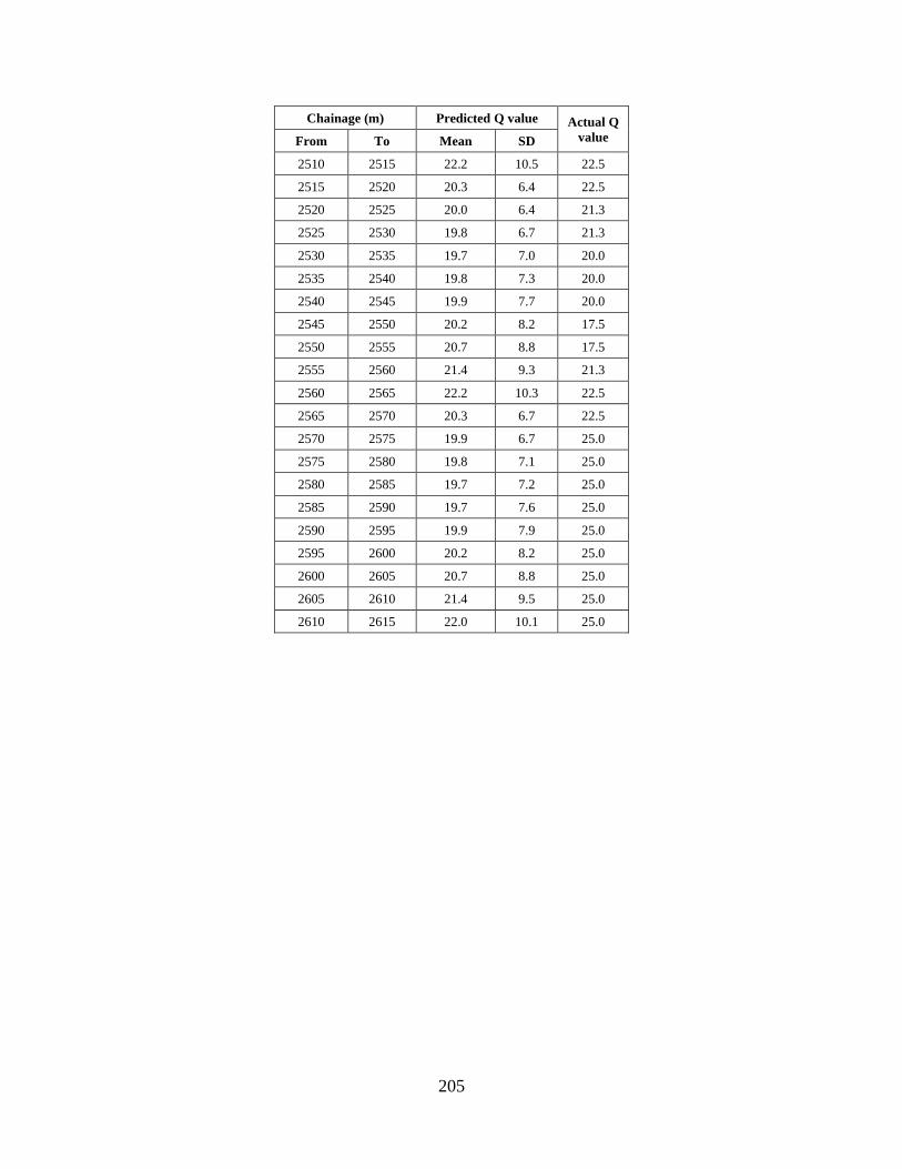
205
Chainage (m) Predicted Q value Actual Q
value From To Mean SD
2510 2515 22.2 10.5 22.5
2515 2520 20.3 6.4 22.5
2520 2525 20.0 6.4 21.3
2525 2530 19.8 6.7 21.3
2530 2535 19.7 7.0 20.0
2535 2540 19.8 7.3 20.0
2540 2545 19.9 7.7 20.0
2545 2550 20.2 8.2 17.5
2550 2555 20.7 8.8 17.5
2555 2560 21.4 9.3 21.3
2560 2565 22.2 10.3 22.5
2565 2570 20.3 6.7 22.5
2570 2575 19.9 6.7 25.0
2575 2580 19.8 7.1 25.0
2580 2585 19.7 7.2 25.0
2585 2590 19.7 7.6 25.0
2590 2595 19.9 7.9 25.0
2595 2600 20.2 8.2 25.0
2600 2605 20.7 8.8 25.0
2605 2610 21.4 9.5 25.0
2610 2615 22.0 10.1 25.0

206
APPENDIX G
Technology Transfer Activities
by
Hui Lu1
Dr. Marte Gutierrez1
1 Colorado School of Mines
Sponsorship
(UTC-UTI and cost matching external sponsors)
For
University Transportation Center for
Underground Transportation Infrastructure
(UTC-UTI)
October 30, 2020

207
G.1 Accomplishments
G.1.1 What was done? What was learned?
• A Markovian Q-based prediction model has been proposed using the MCS technique to
provide the probability distribution of rock mass quality along the tunnel alignment before
construction.
• An MCS-based uncertainty analysis framework in the Q-system has been developed to
probabilistically characterize the uncertainty in input parameter of Q-system and its effects
on rock mass characterization and ground response by applying the MCS technique with
appropriate empirical correlations.
• A reliability assessment with the strain-based failure criterion has been performed using the
FORM (First-Order Reliability Model) algorithm.
• The reliability evaluation procedures were applied on the excavation stability The Shimizu
Highway Tunnel in Japan and the engineering feasibility study of the future extension of the
Eisenhower-Johnson Tunnel in Colorado.
G.2 How have the results been disseminated?
• The results were presented at the 2019 Society of Mining Engineers Annual Meeting, Denver,
Colorado, Feb. 26, 2019.
• One journal paper has been accepted and published in a journal.
• A second journal paper was submitted and reviewed in a journal and is under revision.
• A third journal paper is completed and is under review in a journal.
• The results were presented at UTC-UTI workshops.
G.3 Participants and Collaborating Organizations
Colorado Department of Transportation.
G.4 Outputs
Journal publications
Lu, H., Kim, E, and Gutierrez, M. (2020). “Monte Carlo Simulation (MCS)-Based Uncertainty
Analysis of Rock Mass Quality Q in Underground Construction,” Tunnelling and Underground
Space Technology, 10.1016/j.tust.2019.103089.

208
Conference presentations and proceedings
Lu, H., Kim, E. and Gutierrez. M. (2019). “Probability-based uncertainty analysis of rock mass
quality in underground excavations.” SME 2019 Annual Meeting, Denver, Colorado, Feb. 26,
2019.
G.4 Outcomes
• The proposed Q-based prediction model was shown to be valuable in reducing
uncertainties and risks involved in rock mass classifications and can serve as a
complement to geology exploration in the planning and preliminary design stage of
underground construction. It can also provide insights into the decision support for the
design of excavation sequence and support schemes for the underground structures.
• The proposed framework of the MCS-based uncertainty analysis in the probabilistic Q-
system can provide an approach for systematically characterizing the uncertainty in the
rock mass classification and its propagation to associated rock mass parameters. The
framework can also serve as a useful tool to obtain insightful information for the
probabilistic evaluation of ground responses and support performance of underground
structures.
• The reliability assessment using the Q-based empirical approach can be used as a
complement to analytical and numerical approaches in the preliminary evaluation of the
stability of underground excavations.
G.6 Impacts
• Using the improved tool developed in this research project, tunnel lining design can be
more efficient resulting in more cost-effective, safer and more reliable tunnel structures.