two-stroke cycle outboard engine emissions

%

à«:

»tt.» » REPORT NO. CG-D-122-75

U.S. COASTGUARD POLLUTION ABATEME PROGRAM - TWO-STROKE CYCLE OUTBOARD ENGINE EMISSIONS

a»T %)

T M

R. A. Walter

OOCUMCNT I« AVAILABLE TO THE PUBLIC THROUGH THE NATIONAL TECHNICAL INFORMATION SERVICE, SPRINGFIELD, VIRGINIA »1S1

.4

Prepared for

U.S, DEPARTMENT OF TRANSPORTATION UNITED STATES COAST 6UARD

Office of Research and Development Washington DC 20590

1.1 ,4> ¿mi iAidfeá

L

«i*

«aaMiiiMMiiü»

NOTICE

This docunent is disseminated under the sponsorship of the Department of Transportation in the interest of information exchange. The United States Govern¬ ment assumes no liability for its contents or use thereof.

NOTICE

The United States Government does not endorse pro ducts or manufacturers. Trade or manufacturers' names appear herein solely because they are con¬ sidered essential to the object of this report.

í.

f

ni, %y;

H - H

Technical Report Documentation Page

/c,.

L Author't) - -----

filOjR. A,/ Walter j

2. Cov*fnm*nr Accession No. 3 Recipient • Catalog No

and Subtitle

U . 3. CÜÄ5T GUARD J>OL LUT ION J\B ATEMHNT...PROG RAM tWO-STROKE CYCLE OUTBOARD ENGINE EMISSIONS if. î / < ?

9. Performing Organisation Nome and Address

U.S Department of Transportation Transportation Systems Center w—' Kendall Square Cambridge MA 02142

Î1. Con troc t or G\jdnt No.

CG607/R6^01

12. Sponsoring Agency Nome ond Address

U.S. Department of Transportation United States Coast Guard Office of Research and Development Washington DC 20590

^J^j^ype of Report ajjà Pe nod Covered

Jeeeilsii74^^J * 1^75 i

GDET-1

15. Suppl*m»ntory Not«*

16. XpUract

•^Thii s report documents the results of emissions tests performed on three old and two new outboard engines. Tests of the emissions were made before and after water contact. Older engines were tested in as-received condition, tuned to factory specifications and retested. After being tuned, these engines showed improvements in emissions and fuel consumption. The new engines with improved ignition and combus¬ tion chamber design and crankcase drainage recycling showed less emis¬ sion and better fuel consumption characteristics than the older engines. The results of these tests were used to calculate the emissions impact of the United States Coast Guard outboard fleet for comparison with the emissions impact of other Coast Guard vessels and vessels in general. f*

K

./Cx

S'

j'—. <' i

V

17. Kpy Wardt

Gaseous Emissions, Coast Guard, Ail Pollution, Outboard Engines

19. Security CUttif. («f fhi*

Unclassified

IS. Dittributian Statammt xxxsy

DOCUMENT IS AVAILABLE TO THE PUBLIC THROUGH THE NATIONAL TECHNICAL INFORMATION SERVICE, SPRINGFIELD. VIRGINIA 22161

V . '■\>)

30. St cur I ly Clattil. (af thit pt»P>

Unclassified

21. No. al Ptgtt

136

22. Prlta

Form DOT F 1700.7 (8-72) Rap reduction al complatad papa author! tad

« r L t

/07 0

-.-.-....

PREFACE

The U.S. Coast Guard is engaged in a continuing effort to

minimize exhaust emissions from Coast Guard power plants. This

effort includes investigation of the following related factors:

1. Extent of exhaust emissions to the air from two-stroke

outboard engines as a function of age and operating

condition.

2. Determination of the effect of tune-up on exhaust emis¬

sion and fuel consumption of older engines.

3. Effect of water/exhaust mixing on exhaust emissions to

the air.

This report, sponsored by the U.S. Coast Guard, Office of

Research and Development, describes and analyzes the work per¬

formed and the results obtained during this investigation by the

U.S. Department of Transportation, Transportation Systems Center

(TSC) .

The author is pleased to acknowledge the valuable cooperation

provided through the duration of the project by Cdr. Robert J.

Ketchel, Lt. Roswell W. Ard, and Lt. Cdr. James R. Sherrard, Coast

Guard Project Officers for 1972-1973, 1974, and 1975 respectively.

In addition, grateful acknowlegement is given for the significant

contributions provided by Earl C. Klaubert, Richard A. Roberts, and

Charles R. Hoppen of TSC.

The author would also like to thank James Kelley, Raytheon

Service Company, for his help in preparing and organizing this

report.

PRECEDI Mí PJWI BLANK-NOT FIIWED

TABLE OF CONTENTS

Section

1. INTRODUCTION

Page

1

2. TEST PREPARATION AND PROCEDURE...

2.1 Test Engines. 2.2 Test Cycles. 2.3 Test Cell.

2.3.1 Engine Test Mount. .. 2.3.2 Engine Cooling. 2.3.3 Drive Shaft Assembly 2.3.4 Dynamometer.

2.4 Ancillary Equipment 17

2.4.1 Crankshaft and Propeller Shaft Speed 2.4.2 Fuel Consumption. 2.4.3 Temperature Readouts. 2.4.4 Engine Control Panel.

i 4

2.5 Gas Sampling System...

2.5.1 Gas Sample Probe.••• 2.5.2 Heated Sample Probe Extension 2.5.3 External Sampling Lines.

2.6 Emissions Measurement Instrumentation 30

2.6.1 Specific Instrumentation........ 2.6.2 Exhaust Gas Sampling Conditioning. 2.6.3 Emission Measurement Operation.

2.7 Exhaust/Water Contact System. 2.8 Engine Tests.

2.8.1 Engine Fuel and Lubricating Oils 2.8.2 Engine Preparation. 2.8.3 Emissions Testing.......... 2.8.4 Operating Mode Stabilization.... 2.8.5 Engine Tune-Ups.

2.9 Data Handling and Reduction...

35 37

37 39 41 44 46

46

2.9.1 Computer Data Reduction........... 2.9.2 Water/Exhaust Mixing Data Reduction.

47 53

TABLE OF CONTENTS (CONTINUED)

Section Page

3. RESULTS. 54

3.1 1959 Johnson, 50 HP. 54 3.2 1964 Mercury, 65 HP. 61 3.3 1962 Mercury, 70 HP... 68 3.4 1974 Evinrude, 40 HP. 69 3.5 1972 Mercury, 40 HP. 99 3.6 Water/Exhaust Mixing Results... 99

4. DISCUSSION OF TEST RESULTS. 106

4.1 General. 106 4.2 Engine Tune-Ups. 103 4.3 Water/Exhaust Mixing. 110 4.4 Old Versus New Engines. 110 4.5 Reproducibility of Results. 114

5. EMISSIONS IMPACT. 116

5.1 Outboard Engines in CG Fleet... 116 5.2 Outboard Engine Operating Modes. 117 5.3 Emissions Impact Calculations. 117

6. CONCLUSIONS. 122

7. REFERENCES. 123

vi

aam lÜÉfjAÉ

LIST OF ILLUSTRATIONS

Figure Page

1. Exterior View of Test Cell and Ancillary Equipment... 5

2. Outboard Engine Test Stand. 6

3. Outboard Engine and Lower Unit Enclosure.

4. View of Lower Unit Tank. 8

5. Outboard Engine Water Circulation Layout. 9

6. View of Lower Unit Tank and Drive Shaft. 11

7. Side View of Drive Train. 13

8. Water Brake Dynamometer, Test Cell Interior. 14

9. Performance Envelope of Dual-Rotor Dynamometer. 15

10. Typical Torque Meter Calibration Curve. 16

11. Opto-Electronic Engine Tachometer. 18

12. Fuel Flow Meter Set-Up. 19

13. Engine and Dynamometer Control Panel. 21

14. Exhaust Sample Probe with Major Components. 23

15. X-Ray of Mercury Engine (Side View). 24

16. Heated Sample Probe Extension.. 26

17. Emissions Sampling Line Layout. 28

18. View of Sample Line System. 29

19. Exhaust Emissions Measurement Instruments. 31

20. Flow Schematic for Emission-Measuring Instrumentation 33

21. Water/F.xhaust Mixing Flow Schematic. 36

22. Exhaust Emission Bubble and Level Control Tanks. 38

23. Fuel Storage and Preparation Room. 40

24. Typical Strip-Chart Recording for CO and CO2 at One Power Setting... 4 2

vu

,

""Si

'■i

Î

,, .. . : Ai^iiáfiídââkiHife ----- —..,. . ¡ííMíéiIiíéMb auburn

LIST OP ILLUSTRATIONS (CONTINUED)

Figure ZM®.

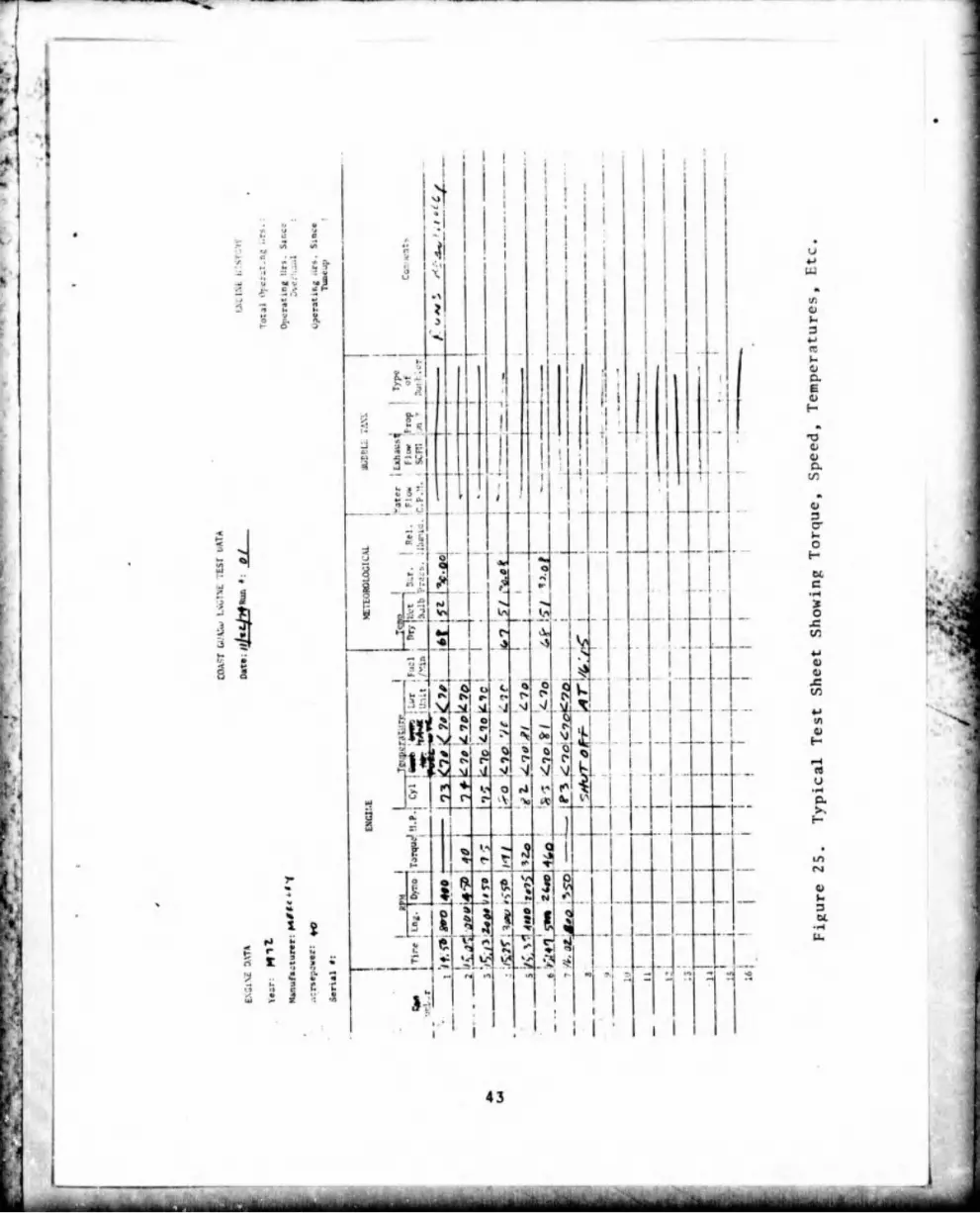
25. Typical Test Sheet Showing Torque, Speed, Temperatures,

Etc. 43

26. Typical Strip-Chart Recording for CO and CO2 after Scrubbing. 4

27. Computer Program Flow Diagram. 51

28. Average CO Emissions Before and After Tune-up (1959 Johnson, 50 HP). 55

29. Average COo Emissions Before and After Tune-up (1959 Johnson, 50 HP). 56

30. Average NOx Emissions Before and After Tune-up (1959 Johnson, 50 HP). 57

31. Average THC Mass Emissions Before and After Tune-up (1959 Johnson, 50 HP). 58

32. Average Percent Fuel Unburned Before and After Tune-up (1959 Johnson, 50 HP). 59

33. Brake Specific Fuel Consumption Before and After Tune-up (1959 Johnson, 50 HP). 60

34. Average CO Emissions Before and After Tune-up (1964 Mercury, 6 5 HP). 62

35. Average CO, Emissions Before and After Tune-up (1964 Mercury, 65 HP). 63

36. Average NOx Emissions Before and After Tune-up (1964 Mercury, 65 HP). 64

37. Average THC Mass Emissions Before and After Tune-up (1964 Mercury, 65 HP). 65

38. Average Percent Fuel Unburned Before and After Tune-up (1964 Mercury, 65 HP). 66

39. Brake Specific Fuel Consumption Before and Aftet Tune-up (1964 Mercury, 65 HP). 67

40. Average CO Emission Rates Before and After Tune-up (1962 Mercury, 70 HP). 70

41. Average CO2 Emissions Before and After Tune-up (1962 Mercury, 70 HP).

viii

LIST OF ILLUSTRATIONS (CONTINUED)

Figure Pag

42.

43.

44.

45.

46.

47.

48.

49.

50.

Average NOx Emissions Before and After Tune-up (1962 Mercury, 70 HP)...

Average THC Mass Emissions Before and After Tune-up (1962 Mercury, 70 HP).

Average Percent Fuel Unburned Before and After Tune-up (1962 Mercury, 70 HP).

Brake Specific Fuel Consumption Before and After Tune-up (1962 Mercury, 70 HP)...

Effect of Tune-up on Fuel Consumption (1962 Mercury. 70 HP)...

Average Mass Emissions (1974 Evinrude, 40 HP).

Average NOx Emissions (1974 Evinrude, 40 HP).

Average Percent Fuel Unburned (1974 Evinrude, 40 HP)..

Brake Specific Fuel Consumption (1974 Evinrude. 40 HP)....

72

73

74

75

76

77

78

79

80

51. Average CO Emissions--Rich Versus Lean Carburetion (1974 Evinrude, 40 HP)... 81

52. Average CO2 Emissions--Rich Versus Lean Carburetion (1974 Evinrude, 40 HP). 82

53. Average NOx Emissions--Rich Versus Lean Carburetion (1974 Evinrude, 40 HP). 8j

54. Average THC Emissions--Rich Versus Lean Carburetion (1974 Evinrude, 40 HP). 84

55. Average Percent Fuel Unburned--Rich Versus Lean Carburetion (1974 Evinrude, 40 HP).. 85

56. Average Mass Emissions (1972 Mercury, 40 HP). 100

57. Average NOx Emissions (1972 Mercury, 40 HP). 101

58. Average Percent Fuel Unburned (1972 Mercury, 40 HP)... 102

59. Brake Specific Fuel Consumption (1972 Mercury, 40 HP). 103

ix

. ■■■>" .--- -,,

t

LIST OF ILLUSTRATIONS (CONTINUED)

Figure Page

60. Comparison of Mass Emissions (3600 HP Diesel - 65 HP .. 107

61. Effect of Tune-up on Mass Emissions (1962 Mercury, 70 HP)...109

62. CO Emission Losses in Water. 111

63. N0X Emission Losses in Water. 112

64. THC Emission Losses in Water... H3

.

LIST OF TABLES

Table

1. 2. 3. 4.

5.

6. 7.

8. 9.

10.

11.

12.

13.

14.

15.

16.

17.

18.

Page

OUTBOARD ENGINES TESTED. 2

APPLIED HP FOR TEST ENGINES. 3

SAMPLE PRINT-OUT. 52

MASS EMISSIONS DATA FOR 1974 EVINRUDE AT MID-CARBURETOR SETTING (LBS/HR). 86

CONFIDENCE LEVEL (901, TWO-SIDED TEST) DATA FOR 1974 EVINRUDE (LBS/HR). 88

MERCURY ENGINE BREAK-IN SCHEDULE. 99

WATER/EXHAUST MIXING RESULTS. 104

EMISSION LOSS IN WATER. 105

OUTBOARD MOTOR EXHAUST EMISSIONS COMPARED TO AUTO EMISSIONS. 106

FUEL SAVINGS BY TUNING-UP 1962 MERCURY, 70 HP, OUTBOARD ENGINE. uo

CRANKCASE DRAINAGE FROM TEST ENGINES IN WEIGHT OF FUEL CONSUMED FOR ENGINE GROUPS OF INTEREST. 114

AVERAGE PERCENTAGE OF UNBURNED FUEL. 115

TIME-WEIGHTED EMISSION FACTORS FOR TEST ENGINES.118

COMPOSITE TEST CYCLE EMISSIONS. 119

BRAKE SPECIFIC MASS EMISSION RATES - COMPOSITE. 120

AVERAGE BRAKE SPECIFIC COMPOSITE MASS EMISSIONS.120

AVERAGE YEARLY EMISSIONS PER TYPICAL DISTRICT FOR USCG OE ENGINE CATEGORIES. 121

YEARLY EMISSIONS FOR USCG FLEET AND OUTBOARDS--121

XI

-

PRECE DI tO Píos blank. ÎSPOT EILMED

1, INTRODUCTION

This report describes the results of exhaust emission tests

performed on two-stroke cycle outboard engines at the Marine

Engine Test Facility located at the Army Materials and Mechanics

Research Center (AMMRC), Watertown, Massachusetts. These tests

provided for analysis of new engines and older engines of the type

commonly used on privately-owned craft. The existing literature on

outboard engine testing has been almost totally directed toward

testing of new engines (see References 1 and 2). Little data has

been available on emissions from older engines which are still pre¬

sent in significant numbers. The test results described in this

report detail the potential for emission improvement of older

engines resulting from engine tune-up. Also, because outboard

engines exhaust below water level, additional engine tests were

included to determine the relative distribution of exhaust pro¬

ducts above and below the water.

Although the results reported apply to a relatively limited

statistical sampling, the data obtained will serve as a data base

for the Coast Guard and other interested agencies.

2, TEST PREPARATION AND PROCEDURE

2.1 TEST ENGINES

The test program involved analysis of five outboard engines,

whose nominal characteristics are indicated in Table 1.

TABLE 1. OUTBOARD ENGINES TESTED

MAKE YEAR RATED HP

Johnson

Mercury

Mercury

Evinrude

Mercury

1959

1964

1962

1974

1972

50

65

70

40

40

Three of these engines were older models, ranging in age from

10 to 15 years. Although total engine hours of use and total

operating hours since the last tune-up were not known, the engines

functioned adequately during performance tests. Information made

available by the former owners of these engines indicated that,

except for winterizing, maintenance procedures, such as engine

tune-up, were rarely performed, and that starting readily and con¬

tinuous operation were the sole criteria for satisfactory engine

performance. Operation under the conditions described is common

for many privately-owned outboard engines; thus, although the

present sampling is limited in quantity, the assumption that these

maintenance conditions are typical for older engines is considered

valid in this discussion.

The exhaust emission tests on these older models provided test

data for two conditions as a basis for comparison: first, for the

original existing condition of the engines at the time of their

procurement; and secondly, for their performance after a tune-up

in accordance with factory specifications.

Two new engines were also tested (after break-in) to compare

these results with the results obtained from older engines in the

untuned and tuned condition.

2.2 TEST CYCLES

The load horsepower applied to the engines tested in this

program followed the generally accepted power curve for planing

hull boats:

P = KfS)2,5

where

P = horsepower

K * a constant

S => engine speed (rpm).

émíMéém

The factor K, which was calculated for each engine at its

rated speed and horsepower, was then used to calculate the load

to be applied at the engine speeds of interest (usually increments

of 1000 rpm). Table 2 gives the conditions of speed and load for

each engine tested. These loads and crankshaft rpm were con¬

tinuously monitored throughout the test runs.

TABLE 2. APPLIED HP FOR TEST ENGINES

SPEED RPM

1959 Johnson

1965 Mercury

1962 Mercury

1974 Evinrude

1972 Mercury

700-800 1000 2000 3000 4000 4500 5000 5200 5500

1.16 6.58 18.14 37.25 50.00

1.05 5.96

16.43 33.73

58.93 65.00

0.937 5.58

15.38 31.57

55.16

70.00

0.93 5.27

14.51 29.80 40.00

0.715 4 .05 11.15 22.89

40.00

uaotiHÈu* UÉÜ

2.3 TEST CELL

The engines were tested in the specially constructed Engine

Exhaust Emissions Test Cell (Figure 1) located in Watertown,

Massachusetts. It is operated by tne Transportation Systems Center

unde the auspices of the USCG >:o test USCG diesels and outboard

engines. The cell was designed to attenuate engine noise and

satisfy the safety requirements associated with operating gasoline-

fueled engines. The cell and its associated instrumentation was

described in a previous report (Reference 3). However, those

aspects of the cell and its associated equipment considered im¬

portant for the understanding of this study will be described

briefly herein.

2.3.1 Engine Test Mount

The outboard engines (OE's) under test were rigidly attached

to a universal support structure or test mount weighing nearly

1000 pounds (Figure 2). This mount provides precise positioning

of OE's with short (15”) or long (20”) shaft engines so that their

propeller shafts are precisely in axial alignment with the dynamo¬

meter drive shaft.

The test mount also contains the lower unit enclosure, fuel

system, and electric start panel. The lower unit enclosure

(Figure 3) contains the water tank which is equipped with adjustable

jack screws for engine alignment. The two-piece tank cover is

attached to the exhaust duct and serves to confine the water

splashed up by the drive shaft and engine exhaust. Figure 4 is

a view of the lower unit tank including the lower unit restraint

plate. Each restraint plate is specially molded to fit the lower

unit of the particular engine under test. Also seen in Figure 4

is part of the recirculation system which pumps tank water past

the OE's lower unit for cooling and to simulate an engine's normal

motion through the water.

2.3.2 Engine Cooling

Figure 5 shows the outboard engine cooling and water cir¬

culation layout. The tank water is constantly resupplied by

. . .«...JuL.«.*... .._... ^-- 1*1. ..

4

ÉÉ

1/ ' 1

i T\J 1 I ! —h ÉÊ in 1 h ! 1 *-1

_:____:-,. ■.: ,■■■■;. ■ .■ -. . ... ....:.........;.. ...... .. .i «. I1. '«.•■ -, -. ■ i.'■ - ■

FUEL FLOWMETER

Figure 2. Outboard Engine Test Stand

LOWER UNIT .ENCLOSURE

Figure 3. Outboard Engine and Lower Unit Enclosure

.....i.;SL.. i '■siinr1

EXHAUST

VENT %

SHROUD

F*:,owi.RM ¡IUNIT■ r.Ncu.osuiu.

RESTJUI

JaCkING SCRLWS

View of Lower Unit Tank Figure 4

fresh water introduced into the recirculation system. Waste water

is drained from the tank at the water surface by a vertical two-

inch standpipe. This standpipe also maintains the water level at

a sufficient height to allow pickup by the engine cooling water

inlet.

Recirculated water flows via a pump, around the engine lower

unit. This serves two purposes: to cool the lower unit and to

assure an adequate water supply for engine cooling at the engine's

water inlet. This feature was found to be especially important for

the new engines where the water inlet was located near the trim-tab

at the aft end of the engine. In this case the engine exhaust

created a vortex in the tank water (more prevalent at high rpm)

so that an insufficient water supply was reaching the OE water

inlet. It was necessary then to extend the recirculated water-

supply inlet by flexible tubing to close proximity with the OE

water inlet.

Because of mechanical condition and deposits in the cooling

system of the older engines, it was necessary to introduce low-

pressure fresh water via the OF. water-flush fitting. This water

flow could be easily adjusted to assure adequate cooling to the

OE cylinder head.

The tank water, lower unit and cylinder head temperatures

were continuously monitored and recorded to verify adequate OE

cooling at all times.

2.3.3 Drive Shaft Assembly

The OE propeller drive shaft was connected, using the

appropriate shear-pin (OMC*) or spline fitting (Mercury), to an

axial-dri^e shaft extension. The female spline fittings were

obtained from a local propeller repair company and machined

adaptors were used to connect the spline fitting to the axial

drive shaft (Figure 6) . These adaptors were keyed into an

aluminum drive shaft extension. This extension was available in

♦Outboard Marine Corp.

10

three lengths to accommodate the different sizes of lower units

encountered in this study. The extensions were fitted and keyed

into the stainless steel axial drive shaft. This drive shaft

passed through a water-cooled shaft seal in the lower unit en¬

closure tank to an axially sliding drive shaft adapter and double

universal joint (Figure 7). The double universal joint drive shaft

protected the dynamometer from angular forces caused by shaft mis¬

alignment.

2.3.4 Dynamometer

The dynamometer (Figure 8) used for power absorption when

testing the OE in this project was a dual-rotor waterbrake device

manufactured by Kahn Industries. Variations in applied torque at

constant rpm were obtained by varying the water flow to the dynamo¬

meter; that is, by changing the depth of the water in the rotor

housing. These changes are possible within the control limits of

the performance envelope given in Figure 9.

The applied torque was sensed by a hydraulic load cell

attached at floor level to a vertical strut on the torque arm of

the dynamometer housing. The hydraulic load cell converted the

dynamometer rotational braking torque to pressure for subsequent

readout on pressure (Bourdon) type gages located external to the

test cell. Two gages were available to indicate dyno torque in

two ranges, 0-900 in-lbs. and 0-9000 in-lbs. The hydraulic load

cell and readouts were calibrated at least daily during OE testing.

Calibration was accomplished by hanging the appropriate weights on

a vertical holder on the dynamometer torque arm. A typical calibra¬

tion curve for the 0-900 in-lb. gage is shown in Figure 10. The

torque readings taken during a test run were corrected by means of

calibration curves.

800

Actual Torque (in.-lbs.)

Figure 10. Typical Torque Meter Calibration Curve

16

2.4 ANCILLARY EQUIPMENT

Ot er ancillary equipment to monitor the operating parameters

of the engine and its working environment will be briefly

described.

2.4.1 Crankshaft and Propeller Shaft Speed

A universal crankshaft rpm monitor (tachometer) was developed

for this program. This universal tachometer was used to monitor

the speed of each engine tested in this program. A chopper disc

of alternately reflective and non-reflective segments was mounted

on the flywheel (or auxiliary accessory at the same rpm) of the

test OE (Figure 11). An opto-electronic sensing head composed of

an infrared emitting diode (IRED) and a photo transistor generated

and detected the light signal. As the flywheel rotated, alternate

reflective and non-reflective segments of the disc were seen by the

light source and its detector, thus producing a pulsed output which

was made compatible with a standard magnetic sensing tachometer

readout. This tachometer has an adjustable overspeed and under¬

speed ignition cut-off to assure engine operation only within the

speed capabilities of the test OE. A momentary switch was provided

to bypass the low speed cut-off when starting the engine.

The propeller shaft rpm was continuously monitored by a

magnetic-type tachometer that was supplied as part of the

dynamometer.

Both tachometers were periodically calibrated against two

stroboscopes at speeds varying from idle (600-800 rpm) to high

speed (5000 rpm). The tachometer readings never varied by more

than +5% from the stroboscope readings and generally were within

♦2%. The propeller-shaft tachometer had a tendency to "zero drift"

and it was necessary to reset the zero at least daily.

2.4.2 Fuel Consumption

Fuel flow to the engine was continuously measured using a

positive displacement-type fuel flowmeter (Figure 12). The fuel

was supplied from one of two standard six-gallon fuel tanks

17

!

r; < ,.:.

Ttf

giiiüM.

., ... ..... . . . . «.J ..J..., . .. ___ .J» ...... .

. __-, ___-¡.I. ■ r __Jiaiiaii^__ ___ ¡■i.tri iiÍM^)tiiti]*ll!útijillÍkíÜiiilliliÍfl!^ÍHÍiÉiiilii£ii3iliiií¡i:ii¿i¿fííii¿iiiiliilÍM¡LÍÍifciiiiilffll¿2Í¿iiiiiBi¿¿tlíiÜSliii

[Figure 2) mounted approximately 20 inches above the fuel flow

meter to compensate for the pressure drop across the meter. The

fuel flow meter has an integrating-type dial readout capable of

reading fuel consumed within 0.001 gallons (^0.068 lbs.) with a

rated accuracy of + 1 percent. To assure accurate fuel flow

readings, the fuel tanks were periodically weighed before and

after each run series and compared with the flow meter readings.

Periodic checks were also made of the weighed fuel versus

the flow meter measured fuel at one of the test engines operating

modes. This assured accuracy over the complete operating

capability of the OE. Generally, weighed and flow meter fuel

consumption readings agreed within _+ 2 percent.

2.4.3 Temperature Readouts

In addition to the tank water, lower unit and cylinder head

temperatures, other temperatures were continuously monitored and

recorded. These included carburetor inlet air, fuel temperature

at the fuel meter, and dynamometer drain water. All temperatures

were measured by thermistor probes that were calibrated daily.

The dry and wet bulb temperatures, as well as the barometric

pressure inside the test cell, were recorded during each test run.

2.4.4 Engine Control Panel

The engine control panel (Figure 13) was located external

to the test cell and contained all the necessary gages and hardware

for monitoring and controlling the engine performance. Readouts

of engine load, speed and operating temperatures were provided.

Water flow meters and valves controlled the applied load to the

dynamometer. An engine throttle control with turn-key engine

starting (for engines with electric start) was located on the

right side of the control panel, as well as an emergency ignition

cut-off switch for rapid shut-down of the engine.

20

1...,,ca»

2.5 GAS SAMPLING SYSTEM

Since gas sampling and conditioning is important to assure

a representative gas sample, each section of the gas sampling

system and its associated instrumentation will be described in

detail.

2.5.1 Gas Sample Probe

The engines tested in this effort were borrowed from private

sources or the Coast Guard; therefore, only a minimum of modifca-

tions to the engines could be accomplished. As drilling into the

exhaust pipe to extract a gas sample would be too drastic a

modification, two types of sample probes were used to extract

a gas sample from the engine by going up through the engine exhaust

outlet.

Figure 14 shows the probe originally developed for this pur¬

pose. This probe was constructed of a thin-wall stainless steel

bellows with minor and major diameters, 0.25 inches and 0.38 inches

that fits inside a similar bellows of 0.40 inches and 0,60 inches

inner and outer diameters. The exhaust sample flowed only through

the small flexible tube while the outer flexible tube insulated

the exhaust sample from ambient conditions. The sample was ex¬

tracted from the exhaust pipe at a point above the introduction of

engine cooling into the exhaust stream by the sample probe-tip

with four radial holes. The sample probe and tip were oven-brazed

to withstand temperatures to 1400° F. The lower part of the probe

was further insulated from the engine cooling water by fiberglass,

asbestos and teflon tapes.

Using mirrors, lights and much patience, this flexible sample

line was inserted through the exhaust outlet to a point where the

exhaust sample could be extracted without being mixed with engine

cooling water. This point varied from a few inches to a foot

below the OE power head depending on the test engine. Correct

probe placement was verified by x-ray examination (Figure 15).

22

Figure 14.

Exhaust Sample Probe with Major Components

Probe

Vertical

Drive Shaft Horizontal

Drive Shaft

Figure IS. X-Ray of Mercury Engine (Side View)

Probe 1 ip

Some heavy hydrocarbons are present in the two-cycle lub¬

ricating oil mixed at a ratio of 50 to 1 with gasoline. The dead

space between the inner a.id outer flexible bellows in conjunction

with the insulating materials kept the sample probe at a suf¬

ficiently high temperature to minimize the possibility of con¬

densation of hydrocarbons on the inner walls of the probe and

thus affecting results. Probe temperature measurements were

performed on the 1959 Johnson 50 HP OE, using four thermocuples,

each spaced 2 inches apart. These thermocouples gave a temperature

gradient from 1100° F at the tip to 600° F at a point 8 inches

below the tip.

Because of the difficulty of probe placement (especially with

through-the-hub exhaust) and x-ray verification, and a tendency of

the thin-wall bellows sampling tube to develop pin-hole leaks due

to thermal stresses, another type of sampling probe was used later

in the program. This second sample probe was 1/4-inch stainless

steel tubing with the exhaust sample inlet end bent at right angles

to the exhaust flow. The probe end had holes drilled into it to

assure a representative gas sample if stratification was present.

In order to position this probe, the OE power head was removed

(a relatively simple procedure) and the probe inserted from the

top of the exhaust pipe. The probe pick-up was approximately

1 inch to 2 inches below the power head exhaust outlet. As was

the case with the flexible probe, asbestos, fiberglass, and teflon

tape insulated the lower half of the probe from the cooling water.

However, since no double wall construction was used, this lower

part of the probe was also resistance-heated using the technique

described in the next section.

2.5.2 Heated Sample Probe Extension

Both of the previously described sample probes were connected

to a sample probe extension (Figure 16) of the same double-wall

flexible-bellows construction. This extension carried the gas

sample from approximately the engine exhaust outlet, through the

tank water, to an external connecting point of the main sampling

system. The extension was wrapped with asbestos, fiberglass, and

25

teflon tape with a final outer layer of shrinkable tubing for

water-resistance proofing. To counteract the cooling effect

of the tank water, the probe extension was heated by current from

a 40 amp, 6.3 v.a.c. variable transformer. A thermocouple sensor

was "teed" into the center of the extension and its output measured

by a temperature controller that switched the heated line on and

off to maintain a minimum temperature of 250° F. When the 1/4-inch

stainless steel sample probe was used, the portion of the line that

was resistance-heated was extended at least one foot up the exhaust

outlet of the OF.

2.5.3 External Sampling Lines

From the exhaust sample probe extension (Section 2.4.2), the

sample line system (Figures 17 and 18) is divided through appropriate

valving to either the water/exhaust mixing bubble tank (Section

2.7), or directly to the emissions measurement instrumentation.

For direct sampling, valves V2 and V5 are closed, allowing the gas

sample to pass through where the sample is divided between the

heated and unheated sections (350° F). The heated section passes

the sample through a particulate filter to a heated line and directly

to the total hydrocarbon (THC) analyzer. The unheated section

carries the gas sample through the proper conditioning elements

to the carbon monoxide (CO), carbon dioxide (CO2) , oxides of

nitrogen (N0X) and oxygen (02) analyzers. (See Section 2.6).

To direct the gas sample through the bubble tank, valve is

closed and valves V2 and V5 are opened. (Valve V3 was open at all

times except when filter F was being changed. V4 was opened when

the exhaust sample flow was directly to the emissions measurement

instrumentation and it was necessary to maintain a flow on the

bubble tank system.) The exhaust sample then flowed through valve

V2 to the particulate filter F-l. This filter protected the stain¬

less steel bellows pump. Filter F-2 was a water trap used in case

excess water of combustion was present in the exhaust sample. How¬

ever, preliminary tests indicated that water was not present in quan¬

tities sufficient to affect the other elements of the system and this

27

,.-. , ....- • . , . . w-.-y ,. r.. ; , . ; .

.. mm h

, ,¾ ï'*' *, I* !|

-¾¾ ■» i-" ** .

* water trap was not used. This minimized the possibility of any of 1 f ' ï *. ',

..v'* the exhaust gases (especially N02) being lost to the water. The

gas sample then passed through a flow meter (FM-1) to the flow

control valve.

A check valve was installed in the system to prevent the

bubble tank water from flowing back into the system. The gas

sample was then bubbled through the tank water (the bubble tank

is described in Section 2.7), and the scrubbed gas sample was

drawn from the top of the tank. The sample then passed through

a flow control valve and flow meter FM-2 and returned to the main

sampling system for subsequent analysis. The sampling line was

heated to assure that the hydrocarbons were removed only in the

bubble tank.

A preliminary test with the 1959 Johnson 50 HP OE and cold

sample probe and lines produced a total hydrocarbon (THC) con¬

centration 10 percent less than that obtained when all lines were

heated. The sample lines and valves that contact the gas sample

(except for the various elements of the bubble tank) were made of

stainless steel or teflon. A purge line that provided processed air

for rapid clean-up of the exhaust sample was also provided.

2.6 EMISSIONS MEASUREMENT INSTRUMENTATION

The exhaust emissions measurement instrumentation is located

external to the test cell in a caster-mounted cabinet (Figure 19).

The theory of operation of this equipment has been described in a

previous report (Reference 3). The measurement techniques, sampling

conditioning, and specific problems encountered when measuring

exhaust emissions from two-cycle OE's will be enumerated, however.

2.6.1 Specific Instrumentation

The gas species that were measured and the instrumentation

contained in the cabinet are listed below:

Exhaust Emissions Measurement Instruments

Gas Species Inst rumentation

Carbon Monoxide (CO)

Non-disnersive infrared analyzer (NDIR)

Carbon Dioxide (co2)

Non-dispersive infrared analyzer (NDIR)

Oxides of Nitrogen (NO a N0X)

Chemiluminescence analyzer with converter

Oxygen Paramagnetic analyzer

(o2) Total Hydrocarbons (THC)

Flame ionization detector (FID) (totally heated)

The instruments listed above provided data on a real-time

basis. The exhaust emissions cabinet also contained all the

necessary plumbing and fixtures to assure proper test sample

conditioning and handling.

2.6.2 Exhaust Gas Sampling Conditioning

Figure 20 is a flow schematic of the emissions measurement

system. The heated sample line goes directly to the totally

heated Flame Ionization Detector (FID). The cold sample line

passes through a pre-filter to a two-coil refrigerator maintained

at 32° F. The refrigerator removes all condensables, especially

water vapor, that may interfere with the subsequent analysis. One

coil of the refrigerator removes the condensables from the NO

sample; the other coil treates the CO, CO2 and O2 samples. If

NOx is to be measured, the gas sample flows through a stainless

steel converter prior to the refrigerator.

The converter was held at a temperature of 1400° F to reduce

all N0X to NO for subsequent analysis by the chemiluminescence

analyzer. The gas sample then flows through particulate filters

to stainless steel bellows pumps. The flow rate is set by

appropriate flow meters and valves prior to analysis by the

appropriate instrumentation. Both the CO and CO2 NDIR analyzers

are heated to approximately 130°F to eliminate the possibility of

water vapor condensing on the NDIR optics.

ar k* t

33

_r; I..,!:...■ ' . ■■J, . . / „ 11 ,___^ li

c o

c (U 6 3 U

IA c

esc c I* 3 i/í rt <L) as c o IA IA

£ w

u o

<4-1

u

rt £ <D X U

S/3

O

O (VI

0)

3 W)

Uh

■ ^ — ■ -»

The system also provides the capability of introducing zero

and span gases to the appropriate instrumentation for ease of

calibration.

Emission Measurement Operation

In general, the instrumentation performed adequately for

the testing of the OE's reported here. However, major problem

areas are considered unique to the two-stroke cycle spark-igni¬

tion engine because of its high hydrocarbon output. The first

problem encountered involved the operation of the FID for

total hydrocarbon analysis. Because of the high hydrocarbon

concentrations it was necessary to remove and clean the FID burner

and sintered metal prefilters more often than normally required.

Also, in some cases, the THC concentration exceeded the upper range

of the instrument; that is, a measured hydrocarbon concentration

greater than 10 percent. In this case it was necessary to respan the

instrument using at least two different concentrations of calibration

gases (normally propane), reset the 10 percent to about mid-range

and draw a new calibration curve for the instrument. This technique

seemed to work satisfactorily.

The second major problem area involved the use of the NOx con¬

verter. Again, due primarily to the high HC concentrations, the

converter had a tendency to "coke up" (excess hydrocarbons are

burned off at high temperatures). This partial burning off was

verified by the water vapor (water of combustion) and the smell of

burned fuel at the outlet of the converter.

The exposure of the converter to this heavily reducing

atmosphere (and possible combustion) had a detrimental effect on

the converter and subsequent NOx readings. It was necessary to

replace the stainless steel converter coil twice during these tests.

Varying the converter temperature from 1200° F to 1600° F had a

marginal effect on this problem. The technique that was eventually

developed to minimize the coking effect was to keep the NOx measure¬

ment time to a minimum and between measurements flush the converter

ütftf Utitt ■ ift.iÉiüiiÜ «Md

34

with air and periodically with pure 02. A periodic calibration

of the converter was performed. However, even with these pre¬

cautions, if the time between sample runs was not adequate for

the converter to recover, inaccurate N0X readings were obtained.

It should be emphasized that this converter problem did not affect

the accuracy of the NO readings. Generally, enough test runs were

made with each engine so that at least one accurate N0X reading

was obtained in each operating mode.

2.7 EXHAUST/WATER CONTACT SYSTEM

As previously mentioned, since the exhaust of an outboard

engine is released below water level, a system was designed and

built to study the effects of water scrubbing on the exhaust

emissions from these engines. The system that was built is

similar to that used by Southwest Research Institute (SWRI)

(Reference 1) with some modifications that contributed to ease

of operation. It was decided to maintain this basic similarity

to compare results. It is not claimed (SWRI agrees) that this

system simulates exactly the real-world conditions encountered

by OE exhaust. However, it did offer a systematic approach in

which many of the variables could affect the scrubbing process,

such as mixing ratesj water temperature and PH, water pressure,

and flow rates could be controlled or measured.

A flow schematic of the exhaust/water contact system is

shown in Figure 21. Supply water was introduced into the system

through a flow control valve and a water flow meter FM-1.

Water flowed through a float controlled by valve V2 into a level

control tank T. The level control tank consisted of a 12" x 24"

plexiglass tank whose long axis was parallel to the floor. The

water from this tank fed the bubble tank where it was mixed with

the exhaust gas. The bubble tank was also plexiglass and similar

in dimensions to the level control tank. However, the bubble

tank had its long axis perpendicular to the floor. A 15-inch high

plexiglass divider in the middle of the tank acted as a weir to

assure that the water through which the gas sample was bubbled did

not recontaminate the incoming fresh water. The exhaust sample and

35

' , ■,,,.- -.. 1..---1 •,, , , , jr .n.;. •• i, ¡¿hjV-».' • •• *•- - -.-- !- i ' •'>

:.. . ft

fresh water sample were mixed on one side of the weir, and the now

contaminated water flowed off the top of that side over the weir

to the opposite side. The water flowed up a 65-inch stand pipe

that, in conjunction with a variable pressure regulator relief

valve V3, maintained a pressure head on both tanks of 65 inches.

The raw exhaust sample entered the bubble tank through the

exhaust system previously described (Section 2.5). Additional

mixing of the exhaust sample was achieved by an engine-driven

propeller (1800 rpm) located at the base of the tank. The exhaust

sample, after water scrubbing, was extracted from the top of the

bubble tank to the emissions measurement instrumentation. Figure 22

shows an exhaust sample being introduced through the water/exhaust

scrubbing system.

2.8 ENGINE TESTS

The experimental procedures followed in the OE test program

are described in detail in this section.

2.8.1 Engine Fuel and Lubricating Oils

The gasoline used in these tests was the controlled standard

fuel Indolene 30 and conformed to Federal emission test fuel

specifications.

The lubricating oil mixed with the test fuel was the OE

manufacturers product recommended for these engines and conformed

to BIA (Boating Industry of America) standards for TCW service.

The oil was mixed at a 50:1 gasolineroil ratio for all tests as

this ratio is now recommended by the manufacturers for use in

all OE's. The only exception to this was during the break-in

period of the new 40 HP Mercury engine. Per manufacturers recom¬

mendations, the lubricating oil was mixed with the gasoline at a

ratio of 25:1. (No emissions measurements were performed during

this period.)

Fuel temperatures were recorded and density measurements were

corrected, if necessary. However, it was found that the fuel, as

it was stored inside, was normally at constant ambient temperatures.

37

The fuel was measured out by volume and weight in the fuel prepara¬

tion room (Figure 23) and the correct amount of lubricating oil

added and thoroughly mixed. The fuel/lube-oil mixture was then

poured into the 6-gallon fuel tank and carried into the test cell.

The fuel tank was primed and the air was bled from the system by a

valve provided for that purpose (Figure 12).

For long tests, a second fuel tank was provided that could be

primed and cut in (by the use of a two-way valve) without engine

shut-down. Small amounts of leftover fuel were drained from the

boat tanks and discarded before a fresh supply of fuel/oil was

mixed into the tank.

2.8.2 Engine Preparation

When an engine was received for testing, it was thoroughly in¬

spected for broken or disconnected mechanical and electrical parts.

On older OE's, the lower unit gear-case oil was drained and re¬

placed with the manufacturers*specified oil. All grease fittings

were lubricated per factory specifications.

For the last three engines tested, the power head was removed

for gas sample line-probe placement. After the power head was

replaced, the probe position was verified by x-ray if necessary.

The engine was again given a thorough visual inspection. The

powerhead shroud was left off so that the tachometer chopper could

be applied to the flywheel. The engine was then mounted on the

test stand and all electrical, fuel line, and diagnostic con¬

nections were made while the OE propeller shaft was aligned with

the dynamometer drive shaft.

The engine was then started in neutral and allowed to idle

until the engine operating temperature was stabilized. During this

time all equipment was checked and a preliminary emissions test was

made to assure that all emissions instrumentation was operating

properly and no leaks were present in the sample lines. (Leaks

were indicated by lower than normal CO, CO2 and NO and higher than

normal O2.) The OE was slowly accelerated in neutral to check

engine performance and operating parameters. OE’s generally are

SCALE

STORAGE DRUM

' FUEL CONTAINER

BOAT TANK

Fuel Storage and Preparation Room Figure 23

.. .

equipped with a shift detent interconnected with the throttle so

that the engine speed in neutral cannot exceed 1500-2000 rpm.

This feature assures that engine speed cannot exceed rated speed I *

(in neutral, no load) and do permanent damage to the engine.

Upon completion of these preliminary tests, the engine was

shut down, the tank water drained and the engine alignment checked

to assure that the OE had not moved because of vibration, mechanical

stresses, etc. All jack-screws and connections were tightened, if

necessary.

2.8.3 Emissions Testing

Upon successful completion of the preliminary tests, initial

emissions test runs were made. The OE under test was run in

neutral at idle speed (normally 600-800 rpm) until stabilized

engine operating conditions were obtained. The engine was then

put in gear and the necessary loads (as per Table 2) applied for

the particular engine under test. The engine speed and load were

slowly increased until these requirements were met. While changes

in engine power setting were being made, the emissions instru¬

mentation were zeroed and calibrated using the appropriate gases.

The engine was allowed to stabilize at the particular power

setting under test for at least five minutes. Simultaneous

emissions and fuel consumption were taken. The emissions data

were recorded continuously on strip-chart recorders (along with

zero and calibration data). Each power mode was held at least

ten minutes (more often 15-20 minutes) after stabilization. During

this time, emissions and fuel consumption were continuously measured.

Fuel-flow data were integrated over time intervals of five or ten

minutes during the emissions tests. Multiple readings of fuel

consumption were taken to assure consistency. The emission measure¬

ments at a power setting were closely monitored to assure stable

operation and reproducible results. A typical strip-chart record¬

ing for CO and CO2 at one power setting is given in Figure 24.

Other important engine-operating parameters, such as torque, speed,

temperatures, etc., were recorded on test sheets (Figure 25).

41

Each engine-power setting was called a mode. The test runs

were usually performed in sequence from idle to full power. For

example, on the 1962, 70 hp Mercury, mode 1 was idle, 700 rpm;

mode 2 was approximately 1 hp at 1000 rpm, etc. Some initial

tests were taken to assure that the sequence of the test runs had

no effect on the test results. That is, the same results should

be obtained if the test run was from low to high power or high to

low power.

When test runs were performed using the exhaust/water contact

system, the runs through the bubble tank were designated "A" runs

and were performed sequentially with the runs measuring the exhaust

products straight from the engine. In other words, the sequence

of tests would be: mode 1 idle, mode 1A idle through bubble tank

and generally briefly back to mode 1, then mode 2, mode 2A, etc.

In this way the effects of the exhaust/water scrubbing would be

compared only with the untreated exhaust measurements taken in the

same test run. It was noted that when a test run was taken through

the bubble tank, it required at least 5 to 15 minutes for the

readings of the exhaust emissions instrumentation to stabilize.

This was caused by the bubbled exhaust products displacing the air

trapped at the top of the bubble tank. The exhaust emissions were

monitored continuously during this time and measurements were taken

only after the emissions stabilized. A typical CO and C02 strip-

chart recording after water scrubbing is shown in Figure 26. Each

test run required 1-1/2 to 2-1/2 hours of engine operating time.

2.8.4 Operating Mode Stabilization

As previously mentioned, the OE under test was allowed to

stabilize for at least five minutes at each operating mode before

emissions measurements commenced. In general, there was very

little drift in engine speed or load once the OE stabilized.

However with the majority of OE's, there was a midspeed range

(approximately 3000 rpm) at which stabilization was extremely

difficult. In the cases where the speed-load drift was such that

valid emission measurements could not be taken, the engine

speed was varied approximately 100 to 200 rpm until stable

44

i

VI operation could be maintained. These changes will be evident in

Section 3 for each individual engine. A minimum of at least six

test runs (most OE's had many more) were taken with each engine.

Each engine then had a minimum of at least three test runs through

the water/exhaust contact system. In the case of the older engines,

the OE was retuned and again tested for a minimum of six runs.

These runs were compared for consistency, and, if necessary,

additional test runs were performed.

2.8.5 Engine Tune-Ups

The old engines (1959 Johnson, 1962 Mercury, and 1965 Mercury)

were emissions-tested in the as-received condition. The engines

were then tuned and retested. The 1959 Johnson was retuned by

TSC personnel as per OMC factory authorized specifications. The

two Mercury OE's were tuned by a factory-authorized Mercury

dealer. The tune-up consisted of the following:

Cylinder compression check;

New spark plugs;

New points and condenser;

Check and replace, if necessary, ignition wiring;

New fuel-pump diaphragm;

New fuel filters;

Check and, if necessary, adjust carburetor;

Check and, if necessary, reset timing.

The engines were tuned-up on the test stand. After the tune-

up, the engine speed was slowly increased while engine operating

parameters and performance were monitored without load. The engine

was then placed in gear and the load slowly applied while emissions,

operating parameters, and performance were monitored. If the

engine performance was acceptable, emissions testing proceeded

as described in Section 2.8.3.

1. 2. 3.

4.

5.

6. 7.

8.

2.9 DATA HANDLING AND REDUCTION

As previously mentioned in Section 2.8, all raw emissions

concentration data was recorded on strip-charts; other pertinent

46

•... .. ..

were engine data of speeds, load, temperatures, fuel flow, etc.,

recorded on separate log sheets. These data were then manually

combined on a work sheet. Emission concentration levels as a

function of speed and load were extracted from the strip-charts

and corrected for zero or calibration variations. For the CO and

C02 NDIR analyzers, the response was not linear over the full

scale operating range of the instrument. In this case, correction

curves were used to change the strip-chart raw data to actual

concentration data. Torque readings were corrected with the

torque calibration curve (Figure 10) and actual engine horsepower

calculated. The fuel-flow readings were converted from gal/hr to

Ib/hr using the correct density values. The brake specific fuel

consumption (BSFC) in lb/bhp/hr was also usually calculated at

this time. AH emissions, fuel consumption, and engine operating

parameters were tabulated with engine test number and operating

mode. These working sheets were used for input of the data into

the computer for final data reduction.

2.9.1 Computer Data Reduction

Computer data reduction converts the raw emissions concentra¬

tion information to mass emission information using standard

equations based on the carbon balance technique.

2.9.1.1 Carbon Balance Technique - The carbon balance technique

computes the mass emissions from the raw concentration data based

on the fact that a mole of hydrocarbons in the exhaust measured as

carbon must have originated from one mole of fuel of formula CxHy.

Therefore, the prerequisites for using this technique are that all

carbon-bearing constituents of the exhaust must be measured and

the hydrogen-to-carbon mass ratio of the fuel must be known.

To use the carbon balance technique all concentration measure

meats must be reported on either a "wet" or a "dry" basis. All

corrected concentration measurements include intake air humidity

and water of combustion. The basis of measurement must be con¬

sistent for all species.

As previously mentioned in Section 2.8, a refrigerator was

used to remove all water vapor for the CO, CO2, NO, N0X and 02

measurements. This water vapor was replaced so that all emissions

concentrations were on a "wet" basis (THC are measured on a "wet"

basis). Equations that performed this correction were developed.

It was necessary to measure the dry bulb/wet bulb temperatures and

determine the water content of the air (percent by volume). The

correction equations are:

200-y(2.055) Cw = cd 200-6 + cdii.üss)(1-LUwru'üy

where Cw - wet concentration and Cd * dry concentration.

(1)

Cd 100 (2) 100 + i.u5!>(C(n + cu2fy

y - % volume of water vapor in the intake air.

These corrected "wet" concentrations were then used in the

following carbon balance equations to obtain the fuel specific

mass emissions (M) in lbs/hr. F is the fuel rate in lbs/hr.

Total carbon (TC) - C0% + C02% + HCI

M(CO) (lbs/hr) * 1.98 (CO%)F/TC

M(C02)(lbs/hr) * 3.11 (C02%)F/TC (3)

M(NOx)(lbs/hr)

M(THC)(lbs/hr)

3.26 (NO xjajm

10

(HC%) F/TC

) F/TC

The constants (1.98, 3.11, 3.26) are based on the atomic

weights of hydrogen, carbon, the components of the exhaust being

calculated, and the hydrogen-carbon ratio of the test fuel.

The fuel-to-air ratio (F/A) may also be calculated using similar equations:

F/A TC W- 2(C0%) - CÖ. (4)

48

It should be realized that the calculated F/A ratio for a

two-cycle engine with large amounts of unburned fuel is not exact,

but is given here for comparison and trend purposes only. Brake

specific mass emissions can then be calculated by dividing each of

the fuel specific mass emissions by the hp at that operating mode.

2.9.1.2 Computer Program - A computer program was developed that

performed the calculations in the previous section and presented

the results in a usable format. A flow diagram for this program is

given in Figure 27.

A data set was stored in the memory by number. The run number

was then coded by month, date, year, and the sequential run of that

day. For instance. Run Number 01-01-75-1 was the first run on

January 1, 1975. After entering the run number, the computer

searches the memory for a similar run number. If the run number

is unique, the program progresses to the data input. If the run

number is already stored in memory, a copy of the data may be

obtained, a new file started, or new data may be entered on the

old file.

Engine information was thèn typed into the program. This in¬

formation included manufacturer, model number, year, hp, serial

number, etc. This data and other important engine operating

parameters were then entered into the program. The data was

corrected from "dry" to "wet" and the fuel/air and air/fuel ratios

calculated and printed-out. The emissions were then calculated and

printed out for mass (Ib/hr, kg/hr) , brake hp (lb/hp/hr, kg/hp/hr) ,

and fuel specific emissions (lb/1000 lb of fuel). Also calculated

and printed out are the kg/TM (mass emission rate/turned mile based

on the propeller pitch) and the percent of fuel unburned. The

percent of fuel unburned is the mass emission rate (Ib/hr) of the

THC divided by the fuel rate (Ib/hr) x 100 percent. After printout,

all data was stored by run number in the computer memory for sub¬

sequent analysis or comparison. Table 3 is a sample print-out for

one run.

49

Figure 27

TABLE 3 SAMPLE PRINT-OUT

Ef ITC P P1JM MO. FOUND TT' . .

11 .; ¿741 . VOU MOUT fi I'I'lPV Of INT fi

TO ST OPT f€ll FILE TO If ♦PUT NEW D

MF P MOrCL

MEPC 40.

vf r#*MOM HF-*riff)iNLE:-. ‘■»‘SEPIOL NO*PE.IUCTIOM POT TC

:344860

mm. rrrPftTioN hoto Ir no rro:

r r-i i Ff ti

. GO

. SG

' .V • . c .00 • u OG .00 5.37 : '• .o* 4.10 . i‘i0 .00 4.10 41- .00 50.00 4.18 315.00 .00

: .00 11.7

14.04 18. It

T IMF

1450 1505 1513 1585

nr, PFT1

80© 1 GOO SHOO

lift TO TEMP

. lO

.71 4. 1 3

1547 1608

000 10. *5 4000 88.86 SfuiU 40, »30

"OO . 10

13 1 3 1 }: I 3 13 13

• fPF c TED C or r EUT FftT I Of ♦ DftT ft ci£ no no:: ft r

3.015 t.. Oc'c

6.03 4.68 . 00

.00

.71

13,1 1 £. 8

i !

r; i :. 4

EMIS LI HP MftSS EMISSION riftTft

LI-: HP-HP PC-HP ML HP-HP LI IOOOLB G TM ‘.FUEL Ml IB

COc 2

1 ?.£E+0O 185E♦GO 386E+0O O44E+O0 O8CE+01 S85E •* Ofi 08IE+00 8438+00 85'3€ +130 484E+00 .:85e +01 6t,3E+01 876E+01 O33E+00 147E-Õ4 153E-04 815E-03 4£4E-03 153E-0£ 85OE-0Ê

1871E-04 000E-01 000E-01 0Ö0E-01 O00E-01 360E-0C' 000E-01 686E-04 575E-01 i££lE-0l 713E+00 632E+00 ¿¿1E+00

,055E+00 ,500E-01

1.13E+01 5. 1.67E+O0 5. 7.86E-O1 1. £.78E-01 1. 4.73E-01 4. 2,41E~01 4. 1.08E+01 4. 2.85E +01 1. 4.14E+00 1. t.8IE+00 3. 1.c'lE+00 6. 7.28E-01 7. 7.18E-01 1. 3.03E+01 1. 4.1ÏC-03 1. 5. ScE-04 l, 4.64E-04 3. 6.78E-04 3. 5.07E-O4 5. 8.37E-04 I. 3,37E-03 1, 0.00E-01 0. 0.00C-01 0. O.O0E-01 Õ. 0.00C-01 0. 5.5IE-04 5. 0.O0E-01 0. 5.69E-03 £. 9.57E+00 4. 1.£8E+00 4. 4.15E-01 7. 1.49E-01 7. 1.41E-01 1. 1.01E-01 1. 8.51E+00 4.

134E-01 4cOE-Ol 480E+00 38IE+00 8O8E+O0 366E+O0 948E-01 337E+00 342E+00 395E+00 011E+00 545E+00 304E+01 376E+00 38 IE-04 384E-04 685E-04 367E-03 £57E-03 792E-08 756E-04 0O0E-01 0O0E-01 000E-01 O00E-01 714E-03 000E-01 578E-04 343E-01 183E-01 771E-01 402C-01 461E+00 838C+0O 313E-01

5.13C40Í 7.58E-01 3. ¢1( -O I l.ttC-M £. 15E-01 1.OSE-01 4.95E+00 1. 34E+01 1.88E+00 8.23E-01 5.48E-01 3.30E-01 3.26E-01 1.38E+01 1.88E-03 C.64E-04 £.10E-04 3.08E-04 £.30E-04 4.48E-04 1.76E-03 0.00E-01 0.O0E-01 0.O0E-01 0.00C-01 c.50E-O4 L1.00E-01 2.58E-03 4.34E+00 5.36E-01 1.88E-01 6.76E-08 6. 38E-08 4.60E-0C' 4.31E+00

4.57E+0C' 4 88E+0C- 5.68€+0£ 4. 1 OE +0C-

. 71E +0c' 5.30E+O8 4.4OE+0C' 1.19E+03 1.18E+03 1.89E+03 1.78E+03 1.18E+03 1.561+03 1.£2E+03 1.671-01 1.68E-01 3.31E-01 9.99E-01 3.£61-01 £. 17E+€*0 1.561-01 0.00E-01 0.00C-01 0.00E-01 0.00C-01 8.97E-01 0.O0E-01 £.301-01 3.87E+08 3.7£t+0c’ £.86E+08 c'.£0E+0£ £.:OE+0£ £.£3E+0£ 3.84E+02

1.O4E-01 :-v81E-0£ 1.21E-01 7.48E-08 1.981- 01 1.48E-01 1.O0E-01 £.-£E-01 £. 181-01 £.761-01 3« £6E - Ol .Otf 01

4. £41-01 £.791-61 3.881-05 3.061-05 7.05E-05 1.8£E-04 £.141-04 5.8£E-04 3.571-05. 0.001-01 0.001-01 0. ¢101-01 0.001-01 c.321-04 0.001-01 5. £41-05 8.821 -02 6.801-02 6.311-02 4.011 - 0£ 5.9.-1-02 5.981- 02 8.761-02

3.601+01 3.441+01 2.691+01 1.951+01 £.031+01 1.981+01 3.571+01 3.601+01 3.441+01 2.691+01 1.951+01 2.011+01 1.961+01 3.571+01 3.601+01 3.441+01 2.691+01 1.951+01 £. 03F +01 1.981+01 9.571+01 3.601+01 3.441+01 2.691+01 1.951+01 2.031 +01 1.981+01 3.571+01 3.601+01 3.441+01 £.691+01 1.951+01 £.031+01 1.981+01 3.571+01

PUN ftGftIN (Y OP N1 ? M END

CPU TIME: 55 SECS. TERMINAL TIME: 0:34*33

52

äaMüi

2.9.2 Water/Exhaust Mixing Data Reduction

The data reduction for the water/exhaust mixing was performed

manually. Following the procedures adopted in the SWRI study

(Reference 1), the mass emissions were calculated on the basis of

a nitrogen balance. This assumes that the total nitrogen mass flow

is conserved through the water/exhaust mixing system. The nitrogen

concentrations before and after water contact are calculable by

subtracting the mole percentages of the known exhaust constituents

from 100 percent. This approach directs that the ratios of

the nitrogen concentration before and after water contact are equal

to the ratios of the total exhaust on a mole basis before and after

contact. The percent loss of each constituent (XL) on a mass

basis can be calculated by:

I X, = 100

(N2 B)(X )

VqxT -Tt 'B

(5)

where : Xg = X concentration before

X^ * X concentration after

N2B * N2 concentration before

N2A = N2 concentration after.

This loss when subtracted from 100 percent and multiplied by the

total mass of constituent X emitted (from carbon balance) will give

the total mass emitted to the air after water contact. That is,

(1001 - I XL) MxB « Mxa where X - CO, C02, 02, NOx, or THC. The

gases can be corrected for pressure by using Henry's law: The

mass of a soluble gas that dissolves in a liquid at a given

temperature is proportional to the partial pressure of that gas

(where molecular dissociation is not involved).

53

IMüdUaaúailtt tá»*.... J

3, RESULTS

This section will summarize the results and present the data

on an engine-by-engine basis.

3.1 1959 JOHNSON, 50 HP

This engine was used as the preliminary "work horse" to check

out and set up the equipment and instrumentation. No data was

available on the total engine hours or the hours since last tune-up.

The engine had a well-used appearance and evidently had had one bank

of cylinder heads replaced recently, indicating a major repair

effort. Late in the test program, an overheating problem was en¬

countered because of a faulty water pump. It was difficult to

maintain the cylinder head temperature below the recommended 135° F,

especially at high loads. However, temperatures up to 150° F were

tolerated with no apparent change in emissions or fuel economy.

It was difficult to hold the set speed with this engine at

2000 rpm. It was also noted that this point gave high emission

rates. This was later attributed to improper magneto-to-carburetor

linkage adjustment. In the as-received condition the maximum

horsepower that could be attained at the rated speed was 44 hp.

Figures 28 through 33 give the average mass emission rates,

percentage fuel unburned, and the BSFC of this engine before and

after tune-up. The higher levels of CO2 and N0X indicated that

the engine was performing more satisfactorily after tune-up.

Also, the engine was now capable of 50 hp at its rated speed.

Although there was no significant change in the levels of CO

and THC (in fact at some speeds they increased), the percentage

of fuel passing through the engine as unburned hydrocarbons de¬

creased due to the improvement in fuel economy as can be noted in

Figure 33. The improvement in fuel economy varied from approxi¬

mately 30 percent at 2000 rpm to a few percent at 4000 rpm.

54

1 ■

..

25

20

43

CC M 15

e w

o u

10

X X X X X 1000 2000 3000 4000

RPM 5000

Figure 29. Average CO2 Emissions Before and After Tune-up (1959 Johnson, 50 HP)

56

—]—¡--—x ■ -----

MÊÊÊÊÊÊÊËÊÊÊÊÊÊÊm - ; .1 ■ ■■''IV 'j'li^!' ’ "lit ’ ' u¡r '' ''"'iia i ,... ..- ,. .. , . ■. .. ; ^,.:1 .i-1, .-,-.---.- -,,,,.. .,.

Figure 31. Average THC Mass Emissions Before and After Tune-up (1959 Johnson, 50 HP)

58

Fuel Unburned

60

50

40

30

20

10

O Before tune-up

A After tune-up

Figure 32. Average Percent Fuel Unburned Before and After Tune-up (1959 Johnson, 50 HP)

± X JL

2000 3000 4000

RPM

5000

59

*

r

"'S*

Figure 33. Brake Specific Fuel Consumption Before and After Tune-up (1959 Johnson, 50 HP)

60

I

3.2 1964 MERCURY, 65 HP

This engine appeared to have had limited use for an engine

of its age. The spark plugs had been changed at the end of the

previous boating season. The engine started and ran reasonably

well, with some roughness noted at low speeds. This engine,

however, would not hold the speed and load at 3000 rpm and it

was usually necessary to cut back the throttle to approximately

2600 rpm to obtain stable operation.

After tune-up, the engine ran smoothly at all speeds (the

original ignition points were in poor condition) and rated horse¬

power and speed were easily obtained. Figures 34 through 39 show

the average mass emission rates, percent fuel burned, and the bSFC

for this engine before and after tune-up. A considerable improve¬

ment in emissions and fuel economy were noted.

61

j-j¿ |||jÿtt'rjirtjiijnhllfMi|j|l¡|tií1|iiÍff! ’ ii’iifíiUltfiiíili I mi 11II n.. .

i. ..

Figure 34. Average CO Emissions Before and After Tune-up (1964 Mercury, 65 HP)

62

____■ -. .._/ a. .

CO, Mass Emissions (kg/hr)

> 4-’

* %

, ■! Ä. ; "> .^. , ; ,,■ V ,,, ■__ .. ;, ', Íí¡|¿¡¿|S

Q Before tune-up

¿\ After tune-up

1000 2000 3000 4000 5000 - 6000

RPM

Figure 36. Average NOx Emissions Before and After Tune-up (1964 Mercury, 65 HP)

o Before tune-up

A After tune-up

_-L. 1000 3000 4000

RPM

Figure 37. Average THC Mass Emissions Before and After Tune-up (1964 Mercury, 65 HP)

2000 _L_ 5000

% Fuel Unburned

80

70

60

50

40

30

20

O Before tune-up

A After tune-up

JL X 1000 2000 3000 4000

RPM

5000

Figur« 38. Average Percent Fuel Unburned Before and After Tune-up

K ¢1964 Mercury, 65 HP)

66

m

il*

f '1

U x: (X x:

Xi

in X)

U. ID m

1000 2000 3000 4000

RPM

5000

Figure 39. Brake Specific Fuel Consumption Before and After Tune-up (1964 Mercury, 65 HP)

67

atfü

3.3 1962 MERCURY, 70 HP

This engine appeared to have had extensive use and had been

run in salt water from the appearances of the cooling system and

lower unit. The only problem noted with the engine was a plugged-

up engine tell-tale for the cooling water. Repeated efforts to

clean out the tell-tale (even with the power head removed) were

not successful. However, with the engine cylinder head temperature

being constantly monitored, this feature was not deemed necessary

for these tests. Initially the engine ran roughly, but seemed to

improve after approximately one hour of operating time. Before

tune-up, the maximum horsepower and speed that could be attained

was 56 hp, at 5000-5100 rpm. From the condition of the emission

instrumentation sample line filters, it was evident that this

engine emitted higher levels of particulate matter than previous

engines tested. As noted with the other engines, the mid-speed

rpm's and loads were difficult to hold and at times it was necessary

to bad off or increase the speeds slightly until stable operation

was attained. At this mid-power range, the THC levels exceeded the

upper range capability (10 percent) of the FID analyzer. In this

case, the instrument was calibrated at a higher range with two

different HC calibration gases and linearity assumed. The FID

was recalibrated to its correct range when the THC dropped below

10 percent.

The engine was tuned (spark plugs and points were in poor

condition) and emissions tests were performed again. Figures 40

through 45 give the mass emission rates, the percent fuel unburned

and BSFC before and after tune-up. The rated speed and power were

now obtained (5500 rpm, 70 hp). The engine performance and fuel

economy were considerably improved. The improved fuel economy is

evident in Figure 46 where the fuel consumption before and after

tune-up is given in mi/gal and gal/hr (a 14-pitch propeller was

assumed).

68

ft ¡iiiiiiiiitii - ■ mil,

3.4 1974 EVINRUDE, 40 HP

The 1974 Evinrude 40 hp was a new engine on loan from the

U.S. Coast Guard. The engine was initially "run-in" on the dynamo¬

meter test stand for approximately 6 hours at varying speeds and

loads prior to emission measurements. The engine seemed to run

rough at low speeds and loads (up to 2000 rpm) but smoothed out

at higher speeds. A check of engine ignition, carburetion and

timing indicated that all was in order. This engine has an ex¬

ternal lean/rich carburetor adjustment and emissions tests were

run with lean mixtures, rich mixtures and the adjustment set at

mid-point (recommended for normal operation). Figures 47 through

50 give the average mass emission rates, percentage of fuel un¬

burned, and the BSFC for this engine at mid-carburetor setting.

Since this engine was new, no tune-up was performed. The results

are plotted in Figures 51 through 55 of the mass emission rates

for rich and lean settings for CO, C02, NOx, THC, and the per¬

centage fuel unburned.

The run-to-run variations in the emission rates of the engines

tested appeared to be excessive. To examine these fluctuations

more closely, statistical analysis was performed on the test

results. Table 4 gives the mean, standard deviation, standard

error, maximum, minimum, and range of the mass emission rates for

the four runs performed on the Evinrude engine at mid-carburetor

setting.

Table 5 gives the results of the two-sided 90 percent con¬

fidence level test.

18

'

I

;

16 - O Before tune-up

Züi After tune-up

14

u X 04 M

12 -

t/> G

ï •H £ ui

a) (A C« X O u

8 “

A

, ! 1.1-1_I I_|_ 1000 2000 3000 4000 5000 6000

RPM

Figure 40, Average CO Emission Rates Before and After Tune-up (1962 Mercury, 70 HP)

70

'■nniiMii

■ u . ¡AiÙMÏÔIm tt •'IrP 1 Ht.Mfcra.'îMiua [.aw

Figure 41 Average C02 Emissions Before and After Tune-up (1962 Mercury, 70 HP)

71

■ÉHi ■.¿ijnr *"'"7"***' itiiMifeiiÉiiàiüiB- ■■ .*..; ..._u_.. d,,. ^hb^^^iÉá.tiráaiiiihMik^^

Mass Emissions (g/hr)

35

30

O Before tune-up

A After tune-up

20

19

18

17

16

15

14

13

12

11

10

9

1000 2000 3000 4000 5000

RPM

Figure 42. Average N0„ Emissions Before and After Tune-up (1962 Mercury, 70 HP)

72

i y.

i * . ÊÊmmSmà

9

8 O Before tune-up

A After tune-up

. 1..I_I_I_» 1

1000 2000 3000 4000 5000 6000

RPM

Figure 43. Average THC Mass Emissions Before and After Tune-up (1962 Mercury, 70 HP)

73

90

JL J_ X X 1000 2000 3000 4000

RPM

5000

Figure 44. Average Percent Fuel Unburned Before and After Tune-up (1962 Mercury, 70 HP)

74

tittidglani L ..■■ --- ..ïAXfa XW ikai --

r 4* , J

«fí.-» ff». ,.1 :,-1 i

ÉÜâfea

10

7 -

i» x: a X £> IA

u u. in co

2 -

1 -

_l_ X 1000 2000 3000 4000 5000 6000

RPM

Figure 45. Brake Specific Fuel Consumption Before and After Tune-up (1962 Mercury, 70 HP)

75

site . ini.I mini rum , -mi....

Based on P ~ S2'® (planing hull) and 14-pitch propeller

Q Before tune-up

A After tune-up

Figure 46. Effect of Tune-up on Fuel Consumption (1962 Mercury, 70 HP)

76

11 .. mi -m mi mirlliltewi ttttiia ÉMdÉki,

"'■1

âiUüÉta

Mass Emissions (g/Hr)

Figure 48. Average N0X Emissions (1974 Evinrude, 40 HP)

78

Fuel Unburned

50

40

30

20

10

J_I_I_L 1000 2000 3000

RPM

4000 5000

Figure 49. Average Percent Fuel Unburned (1974 Evinrude, 40 HP)

79

.. .„-.„.i- - ■■ **~ —JMBmmhUn iiiíi»^M^a^É¿^¿áiflaB;i»a

;4][*‘4

f“

, P* %' tu

3

Figure 50. Brake Specific Fuel Consumption (1974 Evinrude, 40 HP)

0 1000 2000 3000 4000 5000

RPM

CO Mass Emissions (kg/hr)

5000

Figure 51. Average CO Emissions--Rich Versus Lean Carburetion (1974 Evinrude, 40 HP)

81

16

i ;

Figure 52, Average CO2 Emissions--Rich Versus Lean Carburetion (1974 Evinrude, 40 HP)

Figure 54. Average THC Emissions--Rich Versus Lean Carburetion (1974 Evinrude, 40 HP)

xX

O Rich

X Lean

1000 2000 3000

RPM 4000 5000

Æ

't;

0) c >-> 3 X) a 3

V 3 u.

Figure 55. Average Percent Fuel Unburned--Rich Versus Lean Carburetion (1974 Evinrude, 40 HP)

85

::

,1 L^l. lil-úS'aiikli iii »ÉS

!■> .1 .•íífcJtiftlíl&lT -Li.:: ¡K.: .' tííí!iK.)i,.L.. .«,'.1' . iif.-liiríli J,

TABLE 4. MASS EMISSIONS DATA FOR 1974 EVINRUDE AT MID-CARBURETOR SETTING (LBS/HR)

«

i

'ï

VARIABLE MEAN

700 rpm

STD DEV STD ERR MAXIMUM MINIMUM RANGE

CO C02 NOx THC FUEL

1.916 2.689

. 944 E-03 1.987

49 . S 25

. 705E-01 .155

. 687E-04 .186

2.545

.352E-01

.774E-01

.343E-04

.931E-01 1.272

2.010 2.883

. 1OOE-O 2 2.248

52.100

1.844 2.504

. 8 6 0 E - 0 3 1.822

46.400

. 166

.379 . 14 2E-03

.426 5.700

34 >LOAD EV7410

35>ELE

VARIABLE

1000 rpm

MEAN STD DEV STD ERR MAXIMUM MINIMUM RANGE

CO CO? NOv THC FUEL

2.075 4.463

, 129E-02 1.692 37.125

.492E-01 .182

. 878E-04 .138

1.215

. 246E-01

.912E-01

.439E-04

.600E-01 .607

2.141 4.680

.139E-02 1.894

37.600

2.035 4.294

.118E-02 1.593

35.900

.106

.386 . 211E-03

.301 2.700

36>LOAD EV7420

37>ELE

VARIABLE

2000 rpm

MEAN STD DEV STD ERR MAXIMUM MINIMUM RANGE

CO C02 NOx THC FUEL

1.562 12.777

.812E-02 2.119

27.725

.520

.815 . 564E-03

.149

.465

.260

.407 .282E-03 . 74 7E-01

.232

2.249 13.620

. 879E-02 2.220

28.300

1.036 11.700

. 744E-02 1.903

27.300

1.213 1.920

. 135E-0 2 .317

1.000

38>AD EV7430

.-«,C In, . till la. llilteliilllulillllilöllli

86

-..1.1- ..4. tad_

TABLE 4 MASS EMISSIONS DATA FOR 1974 EVINRUDE AT MID-CARBURETOR SETTING (LBS/HR) (CONTINUED)

3 9 > E LE

VARIABLE MEAN

CO C02 NOy T UC FUEL

3.848 20.555

138E-01 2.378

19.375

40>LOAD EV7440

41>ELE

VARIABLE MEAN

CO CO 2 NO, X THC FUEL

12.662 26.877

249E-01 4.362 19.950

42>LOS-AD EV7445

ELE

43>

VARIABLE MEAN

CO C02

NOy THC FUEL

13.787 38.420

.4 26E-01 6.069 21.250

3000 rpm

STD DEV STD ERR

.632 1.361

14 7 E - 0 2 , 795E-01

. 236

.316

.680 . 735E-03 .398E-01

.118

4000 rpm

STD DEV STD ERR

.891 1.570

.623E-03 .395

1.396

.446

.785 312E-03

.197

.698

4500 rpm

STD DEV STD ERR

1.404 1.424

, 117E-02 .565

1.207

MAXIMUM MINIMUM RANGE

4.523 21.830

.154E-01 2.491

19.700

3.013 18.800

124E-01 2.319

19.200

1.510 3.030

, 2 9 5 E - 0 2 .172 . 50 0


13.590 27.800

.257E-01 4.938 21.300

11.860 24.530

243E-01 4.054

18.600

1.730 3.270

144E-02 .8 84

2.700


.702

.712 586E-03

.283

.603

14.990 40.150

.442E-01 6.681 22.600

12.160 36.780

.415E-01 5.315

19.700

2.830 3.370

. 2 74E-0 2 1.366 2.900

87

ÈàâÀM

TABLE 5 CONFIDENCE LEVEL (90¾. TWO-SIDED TEST) DATA FOR 1974 EVINRUDE (LBS/HR)

19 > SAVE EV74AV

OLD FILE - OK? Y

20>LOAD EV7470

21>CONF

VARIABLE: CO

MEAN: 1.91575 STANDARD DEVIATION: 7.J46690E-02 STANDARD ERROR OF MEAN: 3.523345E-02

ONE-SIDED OR TWO-SIDED TEST: TWO

CONFIDENCE LEVEL(S) (¾):90,90

CONFIDENCE LEVEL 90.00%, TWO-SIDED TEST LOWER BOUND: 1.83283 UPPER BOUND: 1.99867

2 2 >CONF C02

MEAN: 2.68875 STANDARD DEVIATION: .154832 STANDARD ERROR OF MEAN : 7.741595E-02


CONFIDENCE LEVEL(S) (1):90,90

CONFIDENCE LEVEL 90.00%, TWO-SIDED TEST LOWER BOUND: 2.50656 UPPER BOUND 2.87094


23>CONF NOx

■Cila

TABLE 5. CONFIDENCE LEVEL (90%, TWO-SIDED TEST) DATA FOR 1974 EVINRUDE (LBS/HR)(CONTINUED)

MEAN: 9.4 36500E-04 STANDARD DEVIATION: 6.B69379E-05 STANDARD ERROR OF MEAN: 3.434689E-05


CONFIDENCE LEVEL(S) (%):90,90

CONFIDENCE LEVEL 90.00%, TWO-SIDED TEST LOWER BOUND: 8.628190E-04 UPPER BOUND: 1.024481E-03

CONFIDENCE LEVEL 90.00%, TWO-SIDED TEST LOWER BOUND 8.628190E-04 UPPER BOUND: 1.024481E-03

24 >CONF THC

MEAN: 1.98700 STANDARD DEVIATION: .186193 STANDARD ERROR OF MEAN: 9.309672E-02

ONE-SIDED OR TWO-SIDED TEST; TWO

CONFIDENCE LEVEL(S) (%) :90,90



25>CONF FUEL

MEAN: 49.5250 STANDARD DEVIATION: 2.54477 STANDARD ERROR OF MEAN: 1.27238



CONFIDENCE LEVEL 90.001, TWO-SIDED TEST LOWER BOUND: 46.5306 UPPER BOUND: 52.5194

89



26>LQAD EV7410

27>CONF CO

MEAN: 2.07500 STANDARD DEVIATION: 4.920027E-02 STANDARD ERROR OF MEAN: 2.460014E-02




CONFIDENCE LEVEL 90.00%, TWO-SIDED TEST LOWER BOUND: .2.01711 UPPER BOUND: 2.13289

28>CONF C02

MEAN: 4 .6300 STANDARD DEVIATION: .182300 STANDARD ERROR OF MEAN: 9.115006E-02





90

.


29>CONF NOx

TWO MEAN: 1 . 287250E-03 STANDARD DEVIATION: 8.778145E-0S STANDARD ERROR OF MEAN: 4.389073E-05

ONE-SIDED OR TWO-SIDED TEST:


CONFIDENCE LEVEL 90.00%, TWO-SIDED TEST LOWER BOUND: 1.I83959E-03 UPPER BOUND: 1.390541E-03

CONFIDENCE LEVEL 90.00%, TWO-SIDED TEST LOWER BOUND: 1.183959E-03 UPPER BOUND: 1.390S41E-03

30>CC<-ONF THC

T MEAN: 1.69225 STANDARD DEVIATION: .137909 STANDARD ERROR OF MEAN: 6.895454E-02





31>CONF + LOAD EV7420

TABLE 5. CONFIDENCE LEVEL (901, TWO-SIDED TEST) DATA FOR 1974 EVTNRUDE (LBS/HR)(CONTINUED)

72>CONF CO

MEAN: 1.56200 STANDARD DEVIATION: .520412 STANDARD ERROR OF MEAN: .260206

ONE-SIDED OR TWO-SIDED TEST: TWO,90,90


CONFIDENCE LEVEL 90.00%, TWO-SIDED TEST LOWER BOUND: .949639 UPPER BOUND: 2.17436

CONFIDENCE LEVEL 90.00%, TWO-SIDED TEST LOWER BOUND: .949639 UPPER BOUND: 2.17436

33>CONF C02






34 >CONF NOx

MEAN: 8.121250E-03 STANDARD DEVIATION: 5.640877E-04 STANDARD ERROR OF MEAN: 2.820438E-04



fggg ¡tata tonto totoeto

92




35>CONF THC

MFAN• 7 11Q 2 S STANDARD*DEVIATION: .149384 STANDARD ERROR OF MEAN: 7.469201E-02





36>CONF+ LOAD EV73-430

37 >CONF CO

NOT A VARIABLE NAME.

VARIABLE: WO


VARIABLE: CONF CO


VARIABLE: CO


'S'

93

.. .

llffi

B, I f

I.lrli

f IM

lilÉ

Üi UM

TABLE 5. CONFIDENCE LEVEL (90î , TWO-SIDED TEST) DATA FOR 1974 EVINRUDE (LBS/HR)(CONTINUED)

VARIABLE: LIST


VARIABLE: CO:

MEAN: 20.5550 STANDARD DEVIATION: 1.36050 STANDARD ERROR OF MEAN: .680251





38 >CONF CO






39>CONF NOx


94

nnm 4 . V iVj. '

r . .1 - V8l;-“n

.

j ! j

Jd

Éüri .

TABLE 5 CONFIDENCE LEVEL (90%, TWO-SIDED TEST) DATA FOR 1974 EVINRUDE (LBS/HR)(CONTINUED)



CONFIDENCE LEVEL 90.001, TWO-SIDED TEST LOWER BOUND: 1.211831E-02 UPPER BOUND: 1.557669E-0 2

CONFIDENCE LEVEL 90.00%, TWO SIDED TEST LOWER BOUND: 1.211831E-02 UPPER BOUND: 1.557669E-02

4 0 >CONF THC

MEAN: 2.37775 STANDARD DEVIATION: 7.950419E-02 STANDARD ERROR OF MEAN: 3.975210E-02





41>LOAD EV7440

42 >CONF CO





''i -'j

95

,. ÉMüÉtti

TABLE 5. CONFIDENCE LEVEL (90*, TWO-SIDED TEST) DATA FOR 1974 EVINRUDE (LBS/HR)(CONTINUED)


43>CONF C02






44 >CONF NO,






45>CONF THC

MF AN * 4 250 STANDARD’DEVIATION: .394726 STANDARD ERROR OF MEAN: .197363

96

It,?:

;», r,.





CONFIDENCE LEVEL 90.00%, TWO-SIDED TEST LOWER BOUND: 3.89803 UPPER BOUND: 4,82697

46>CONF f LOAD EV7445

47 >CONF CO






4 8>CONF C02




97

■ . -m, rAi Ll V ¡árf'- '"V

TABLE 5. CONFIDENCE LEVEL (90%, TWO-SIDED TEST) DATA FOR 1974 EVTNRUDE (LBS/HR)(CONTINUED)



4 9 >CONF NOx




CONFIDENCE LEVEL 90.00%, TWO-SIDED TEST LOWER BOUND; 4.118954E-02 UPPER BOUND: 4.394546E-02

CONFIDENCE LEVEL 90.001, TWO-SIDED TEST LOWER BOUND: 4.118954E-02 UPPER BOUND: 4.394546E-02

50>CONF THC

MEAN; 6.06950 STANDARD DEVIATION: .565163 STANDARD ERROR OF MEAN: .282582



CONFIDENCE LEVEL 901, TWO-SIDED TEST LOWER BOUND: 5.40448 UPPER BOUND: 6.73452


98

lü . i.

3.5 1972 MERCURY, 40 HP

The 1972 Mercury engine was new and required break-in as per

Mercury specifications. The engine break-in schedule is given in

Table 6.

TABLE 6. MERCURY ENGINE BREAK-IN SCHEDULE

Speed (rpm) Load fhp) Time (hr)

1000 2000 2500 1000 2000 3000 4000 5000

0 .00 0.00 0.00 0.75 4 .00

11.00 22.00 40.00

1 1 1 1.5 1.5 2

. 25

.25

Speeds above 3000 rpm were maintained for as short periods as

possible.

This engine ran smoothly over all power ranges. As with the

new 1974 Evinrude, no tune-up was performed on this engine. The

mass emission rates, percent of fuel unburned and the BSFC are

given in Figures 56 through 59.

3.6 WATER/EXHAUST MIXING RESULTS

Using the equations given in Sections 2.9.2 and 2.9.3, along

with temperature, pressure and corrections for water content of the

gases, the average losses by mass to the water of CO, CO2, N0X, and

THC were calculated. These loss percentages were then multiplied

by the previously calculated mass emission rates (g/hr) to obtain

the emissions retained in the water. The remainder of the emis¬

sions were discharged to the air. All the water mixing experiments

were conducted with tuned engines, and a four-hole bubbler in the

mixing tank. The water/exhaust mixing ratio was held constant at

4.45. The results of these experiments are given in Table 7. Table

8 shows the percent loss to the water for each of the emissions.

99

Figure 56. Average Mass Emissions (1972 Mercury. 40 HP)

100

,4? ■ * *'

% <.»

1000 2000 3000

RPM

40000 5000

Fu

el

Unburn

ed

50 _

40

30

20

10

1000 2000 3000

RPM

1 4000 5000

Figure 58. Average Percent Fuel Unburned (1972 Mercury, 40 HP)

102

MKtr

U

eu

x> I/) x¡

U U» (/5 03

5

1000 2000 3000

RPM

4000 5000

Figure 59. Brake Specific Fuel Consumption (1972 Mercury, 40 HP)

103

r.u. ki-U <U;.> u,: «»4

TABLE 7.

WATER/EXHAUST MIXING RESULTS

dH Of '3¿6I ahnoahw

dH Of ‘f¿6t HQÍIHNIAH

dH 0¿ ‘J961 AHODHHW

dH S9 ‘f96I AHHDHHW

dH OS ‘6S6I NOSNHOr

dH Of *Z¿6I AHÍIDHHW

dH Of ‘f¿6l HCIflHN ! AH

dH 0¿ ‘?96T AHflSHHW

dH S9 ‘f961 AHnOHHW

dH OS ‘6S6X

NOSNHOf

dH Of ‘e¿6l AHHDHHW

dH Of ‘f¿61 3Gf)HNIA3

dH 0¿ ‘Z961 AHnOHHW

dH S 9 ‘f961 Aanoasw

dH OS '6S6I

NOSNHOf

o cr. oc o cr> i"- o T

00 1^- Ov ««T •t O ^ rsi CTi i<0 •

dD r tn o-. rO O O O 00 LO . K1

-C rr l O 40 l^-. 00 CTi CTi cr. r. • tn

O'. OO r-- ro o «* • r- o o o ro r- j

af) m* so at) io oc «*r ch lO O-. • ■»f

sO f'J -O Oí r- Tt a. Oï «et <7v

•T dD • »—• «-T r« j r—«

■ LO O i rO OA

O 'pf lo cr. en r- i lo oo

•T i-O lO LO LO «t *r r— lo ro • o

r-< OO TT Oa r-> rsi oc r j lo • d3 O r- i ro r-.

lo oo io f r- o * lo r j . X oo ro ao *

O LO r—1 f 00 sO í

•t »-« *t >£) f- OO • f-* rO rO O vC

r -'j ro r-- OJ ro 'tí- «rt ro lo • t-^

cr. ro *t a. rsi OA LO O f' ■*» .o

en o ro --r f'- .lo o r-- r— »T

sO r - lo r - lO o í o lo r-1 t—l «LO *rr f'.-i o 1

r- lo -f en r- c lo o ao —i • «t- lo rg rsi «y

r^- lo lo io rg r-- en r-i 04 sC •.O 00 rg r>~- ^y

ro 00 cg oo LO «rr LO 00 oe en . ro lo ro «y

rvi rg rg io rH dD rH rO

O •--< rg o V© rg i-t

rg ro © sO O ro ro r- j lo en • *y

rg o

«y ro lo i-h .-H en r^- ^y •y «y •

«y © o lo © r-» © LO © 00 .00 r-« © rg

rH rg r-. r-' en lo . r^ -4 n- o o

© lo ro -y ^y O rg c- rg O • »y

rH ©

lo lo ^y rg ^y rg lo rg r- • ro

O

rg en «y rg ^y © rg lo .-11--. • »y

«y ©

*y co "y ro lO rg r-. 00 lo en • ^y

r- —r

rg en © © © © r- en © o • © rH O ro

r- © rg oa ro O 00 O 00 r- . ro —< «y © —<

© ro ^y O © 00 • rg ro «y o OA

O © LO , rg n- lo » lo © . .

04 © ,

© r- - lo lo -y O © ro 00 LO • rH

tO rg rg

© © rg © © rg rg rg cg oo • —• _g co rg rg

LO rg lo en rg en © rg © rg •ft © rg rg

gy lo en oo r- rg to © gy oo • ro

gy lo -g

© gy © rf oo gy • ro ro r- © en

c- ro h- ro rg © r- ro gy © . ©

ro © rg

«y © © gy rg lo ro r-- © o- . rg

LO rg rg

rg rg © —< rg ro © ro rg pg . © pg OA rg rg

C- © rg oc © O 'O o fO oo • LO 00 lO LO rg

rg O rg r- O ro • © rg rg rg io

gy oo lo ro «y © ro gy ro © • © © rg

tO lo © rg rg gy © gy rg rg . ©

ro lo lo lo r- rg © rg

r- rg oo rg gy LO © rg r- O • «y rH © rH

O © rg © lo • © lo rg o lo

© © rg © lo © . © lo gy © ro

O O LO LO O 00 O gy ro • lo r-g ro O r-.

O © 00 LO o . o rg O ro lo rg © r-

LO O O © LO LO © © . gy © © LO rH

O © 00 © O © » LO rg oo o © gy ro rg rg

O O gy O © © • O © rg © ©

© © © © LO © . © © rg o r-

© © r- o © LO .LO r-. r-. rg ©

© © rg lo lo o . r- f- LO © O

© © rg © LO © . LO r- rg rg © LO rg rH rg

O O ro © LO O . © rg gy © lo © r- rg rg

© © lo © ©©•-.© rg © • r- rH rg rg

O O rH © © © « © © © rg ro rg rg rg

© © LO © O LO • LO gy oo rg r-.

© O LO © © o . © lo gy gy oo n- oo ro

O O oo O O © .LO LO LO O © © ro rg ro

O © © O O CD . CD © rg rH r- tg O rg ro

A rg

O lo O © © rg . to r— rH rH LO

© LO rg © lo rg .oo r- ©> rH r-

ro rH

O O lo © LO LO «LO ro r- rg rg rH © rg

© LO LO © LO rg .o © © gy r- gy O rg

© O © O LO O .LO © © rg rg © 00 rH IO

O o . O

fx. LO

o o © © LO © .LO 00 © rg © rg r-- to

O LO O O O rg . © •o rH ro rg gy © ro

O O LO O O LO .LO O rg gy O r- © fx.

o © © © © © .LO O LO 00 fH O rg ©

© © LO O © © . o © © 00 00 fx- © rH LO

LO I ©

rg

rg XJ OOOI U U 2 H

rg XJ O O O X U U 2 H



rg XJ O OO X U U 2 H


'g

104

__ MÜÚi íÉlãiflHÉÉÉilt

105

a, ac

>* Oí o aa ^ u Q¿ * tu rvj T. r-

CTí

{X r:

tu Q O CD «=r

5?: - H-t > w en

Cu aa

>- oc o D r^- U fy* •> tu rs| S o

cr.

cu X

>* Di LO aa o u Di •* yj X vo

Oí

Da X

X O O tO un z X “ O 0¾ »-5 un

en

oo 1-- o un <rt CT\ hO r-U

O \0 tO r-í rM f-u ro

un on r-« o O 00 r^n 00

o un »-H to r-4 IT) t—i <X

00 en en r-n o oc en

un ro r a tO rH *rf Un

«rt O fNJ fM O0 sO un

o% r- en to r 4 00 un un

OO 04 ro 0C "rf un

ro r-H o 00 fO en Tt un

'O en \D oo to 00 «T un

00 un 00 «ni 0-4 00 un

O 04 ru O ro o- en r-

sO 04 00 00 sO O 04

to «rf rf 04 CTí 00 un

r- un \0 ro \D o en

o Tf un i— on o 00 o

O 04 ro un Tf un ro 10

o- to » 04 04 00 LO LO

un I-H o o 04 00 rf

o 04 to r- 04 00 r—< yf

•--t to 00 '■er 10 00 04 rf

00 04 to r-a 04 00 to LO

on Tf un 04 04 00 to un

O O- IO 04 un f-H o un

o en un un un o to

to r-i O- 04 04 ro on

04 on o 00 rH tO 04 vO

Tf Tf tO Tf r- 04 o un

O Tf VO LO O- fO vO IO

O Tf 00 ro to r- Tf un

LO rH O rH 04 r- un o

en 04 04 43 f-H O- Tf un

so en o- un r-i O 04 un

en o en o O- rH Tf

ro ro un un o- 04 ro

\0 O 04 tT rH 00 On 04

o 04 r- so en ro 00 o

ro 04 on rH O 4 ro Tf 4D

r-. un 04 rH 00 Ci vO Tf

LO P*» rH O LO 00 SO O

vO un ro 00 LO 00 SO LO

VO LO Tf sO Tt 00 un un

Tf un ro o Tt 00 Tf

lo ro rH en rH 00 00 rO

00 0- VÛ VO un 00 Tt Tf

LO rH O LO r-l 00 (N tO

rO 00 rH O sO 00 LO O

r- rH 00 00 o r- un un

vO un en Tf o 'O \0 r-i r~4

Tf Tt 43 4D O CvJ LO Tf

en <*4 O 00 00

vO LO O 00 4D en Tf on <m rvj ro

r- Tf o en Tt rH

r- 43 un o r- Tf rg

'O r- ro o- rH l"» Tf ro

o- oo en rH r- (M

04 o un Tt 04 00 04

04 t-* Is- 00 o un

Tf rH Tf 00 \0 I

04 04 XJ oooi oooæ UUZH UUZH

XJ (NI XJ (NJ XJ (N KJ OOOX OOOX O O O X O O O X UUZH UOZH UUZH UUZH

DISCUSSION OF TEST RESULTS

4.1 GENERAL

The emissions observed here are characteristic of over-

scavanged, two-stroke cycle OE and the results are in generally good

agreement with those reported by others (the older engines tested

had crankcase exhaust drainage). In order to develop a better per¬

spective on the mass emission rates from these engines, the CO,

THC, and NOx from the 1964 Mercury 65 hp engines are plotted

against the emissions from a Fairbanks-Morse turbocharged 3600 hp

diesel engine in the U.S Coast Guard service (Figure 60).

The CO and THC mass emission rates (kg/hr) of the 65 hp OE

were approximately twice as high as the CO and THC from the 3600

hp diesel engine. The N0X from the diesel engine, however, greatly

exceeded that from the OE (diesel = kg, OE = g). These high NOx

levels from the diesel are indicative of the high flame temperatures

in the combustion process.

Table 9 compares the exhaust emissions from the OE's to an

average automotive gasoline-powered light duty vehicle. The pre-

1968 automotive emissions are compared to the 1964, 65 hp

Mercury and the 73-74 automotive emissions to the 1974, 40 hp

Evinrude. Units are in grams per mile (g/mi) .

TABLE 9. OUTBOARD MOTOR EXHAUST EMISSIONS COMPARED TO AUTO EMISSIONS

Pollutant Auto(pre-1968)

g/mi

1964 Mercury 65 hp (range) g/mi

Auto(1973-74) g/mi

1974 Evinrude 40 hp (range) g/mi

CO

THC

NOx

88.3

7.82

3.33

80 - 210

210 - 97

0.1 - 0.4

19

2.7

2.3

170 - 219

183 - 98

.08 - .65

I»

Mr' ' ® I . i,"’'’

■ ^ ; %■

Figure 60. Comparison of Mass Emissions (3600 HP Diesel - 65 HP OE)

107

ti

. ..

à '¡'î jyjajfe i, ü

As with the diesel engine, the OE exceeded automotive engines

in mass emission rates for CO and THC, but was considerably less in

N0X. These emission comparisons, however, do not take into account

losses to the water for the OF.

4.2 ENGINE TUNE-UPS

The results of the engine tune-ups on the older OE's tested

were positive. All older engines showed varying improvements in

emissions (except C02 and NOx) and fuel consumption after tune-up.

The increase in the levels of C02 and NOx after tune-up are in¬

dicative of improved combustion efficiency. The improvements varied

from a few percent to 20 percent. The mass emission rates for the

1962, 70 hp Mercury before and after tune-up are given in Figure 61.

The improvement in fuel economy is given in Figure 46. The pol¬

lutant showing the most improvement is THC (25 percent - 40 percent) .

CO shows an improvement generally less than 10 percent. The levels

of N0X increased 50 percent to 100 percent. However, it should be

emphasized that on an absolute basis, as the levels of N0X are ex¬

ceedingly low compared to CO and THC, tune-ups are effective in

lowering emissions.

There is no dramatic decrease in the brake specific fuel con¬

sumption (BSFC), as shown in Figure 45. However, the fuel savings

are more evident in Table 10, where fuel consumption (gal/hr) j.

shown at various rpm and loads before and after tune-up. It should

also be remembered that this engine could not attain rated speed

and load prior to the tune-up.

Further tests should be performed to isolate the particular

elements of the ignition-fuel system that contribute to increased

emissions and fuel consumption and the degradation of these elements

with time. However, it is evident that periodic tune-ups, are cost-

effective in fuel savings and improvement in emissions and environ¬

mental quality.

108

♦if,'] r #

' *•

: % -Í..M ; %• i

"’ursaaihr.-i

20

18

16

14

12

10

Figure 61. Effect of Tune-up on Mass Emissions (1962 Mercury, 70 HP)

109

s

Wi,iiin<[lniàitlttéH!tlMÍWlàJhll'»i[iM*i¡ ir, ul..MtttUliiyiiÉÉ

NO

Mass Emissions (g/hr)

«».■....

i km

* t TABLE 10, FUEL SAVINGS BY TUNING UP 1962 MERCURY, 70 HP, OUTBOARD ENGINE

RPM FUEL CONSUMPTION Before tune-up After tune-up

(gal/hr) (gal/hr)

05 IMPROVEMENT

1000 2000 3000 4000 5000 5500

1.62 2.80 3.46 4.25 5.32

1 .35 2.45 3.29 3.92 5.32 6.47

20.0 14.3 5.2 8.4 0

4.3 WATER/EXHAUST MIXING

Large variations were noted in the engine-to-engine results in

the water mixing experiment. Some of these variations were ex¬

pected as the initial concentrations introduced into the water

tank varied by factors of 20 or more. Figures 62 through 64 show

the emissions in kg/hr lost to the water for each engine tested.

Except for the 1964 Mercury 65 hp engine for CO, the results show

larger losses to the water with older engines which have higher

total emissions.

A review of the results with the Mercury 65 hp indicated that

problems were encountered with the CO NDIR analyzer at the time the

water mixing experiments were performed. This could account for

the lower readings of CO concentrations after water mixing with the

subsequent apparent increase in CO losses to the water. In

general 20 percent - 30 percent of the CO is lost to the water,

80 percent of the C02, and 30 percent - 60 percent of the THC.

Although these water losses are higher than expected, the

general trends agree with the expected solubilities of these gases

in water.

4.4 OLD VERSUS NEW ENGINES

Considerably lower emissions were evident from the new

engines tested in this study. This can be attributed, in part,

to improved combustion chamber design and ignition systems, and

crankcase drainage recycling.

110

f. '-r‘‘j±v" • . - .JßfeUi'V ■" j . ; ,

.'.

:;*ÍH

It

Figure 62. CO Emission Losses in Water

111

h

V ' M

Í

nil.lliiiiliMilliililiill

2000 1000 3000 4000 5000

RPM

Figure 64. THC Emission Losses in Water

113

A recent study conducted by SWRI for EPA (Reference 4) gave

the crankcase drainage from older test engines in weight percent

of fuel consumed by groups according to manufacturer and horse¬

power range. The average results for the older engines of in¬

terest here (1959 Johnson V-4, 1965 Mercury 4 cylinder and 1962

Mercury 6 cylinder) are given in Table 11.

TABLE 11. CRANKCASE DRAINAGE FROM TEST ENGINES IN WEIGHT OF FUEL CONSUMED FOR ENGINE GROUPS OF INTEREST

Group Description

Drainage in Weight Percent of Fuel Consumed

Idle Low Speed

Low Mid

High Mid

High Speed

OMC V-4

4 and 6 cyl. Mercury

31.2

2.16

26.9

1.48

6.48

0.512

4.39

0.126

4.84

0.053

The higher emissions from the older engines could be due, in

part, to worn piston rings or valves. In this regard, compression

checks performed prior to testing of these engines gave readings

well within acceptable limits. The improvement noted with new

engines is demonstrated in Table 12 which gives the percentage of

fuel measured as unburned hydrocarbons for the three older engines

(averaged before tune-up) and the two new engines.

The improvement ranged from 110 percent at 5000 rpm to 23

percent at 700 rpm (idle). Similar improvements were noted in

the CO levels. However, as with tuned older engines, the N0X

levels increased because of more efficient combustion.

4.5 REPRODUCIBILITY OF RESULTS

As previously mentioned, the run-to-run reproducibility did

vary from engine to engine. The 1962 Mercury results had the best

run-to-run reproducibility and the 1959 Johnson had the worst

114

- ■ -.. ■■ ■ -.

' J . LiOjV II , , Jj

TABLE 12 AVERAGE PERCENTAGE OF UNRURNED FUEL

RPM Old Engines New Engines %

Improvement

700 1000 2000 3000 4000 5000

54.0 50.5 51.6 41.0 29.5 27.0

44.0 35.5 27.5 19.5 20.0 21.5

23.0 42.0 87.0

110.0 47.5 25.5

reproducibility. The statistics presented in Section 3.4 on the

1974 Evinrude were typical and proved to be much better than ex¬

pected. These tests seem to indicate confidence in the results

reported herein.

115

..... ik ï Ü à if hiiiilAiiiiiifl un w -¾ r . -■ ..J... ,.-...=

5, EMISSIONS IMPACT

It should be emphasized that any emissions impact based on the

results of this study are estimates only and are based on assumptions

where hard data is lacking.

In order to evaluate the emissions impact of the Coast Guard

outboard engines, the following information was needed:

1. Outboard emissions as a function of speed and load;

2. Numbers and sizes of engines in the Coast Guard fleet;

3. Coast Guard outboard engine operating modes, i.e., time

vs. speed and load;

4. Total operating hours.

Using the data presented in the preceding chapters on out¬

board emissions, a systematic approach was developed to evaluate

the Coast Guard outboard fleet emissions.

5.1 OUTBOARD ENGINES IN CG FLEET

Through conversations with district personnel, it was de¬

termined that each district has approximately 100 outboard engines.

These engines vary in size from 10 hp to 85 hp. The population mix

as a function of hp is approximated as follows:

HP

10 20 40 65

>65

% of Engines at Given HP

10 15 10 60 5

The widely used 65 hp engine powers the popular Boston Whaler.

Assuming the same distribution in each district, about 1000

outboard engines exist in the Coast Guard fleet.

S.2 OUTBOARD ENGINE OPERATING MODES

f*.

I *

§

Data was developed by OMC (as reported in Reference 1) on

outboard engine usage that shows percent of time in rpm intervals

as a function of engine size, boat length, and type (runabout,

cruiser, fishing, etc.). The data for cruiser/runabouts with

50 hp engines will be used in this study as they more closely

approximate the average Coast Guard usage and engine size. These

data were further regrouped for this study into rpm intervals that

correspond to those of the engines tested here. These results are

given below:

RPM % of Time in Mode

idle 12 1000 12 2000 17 3000 12 4000 36 5000 5 5500 6

These percentages, expressed in decimal form, are used to

develop time-weighted emissions and power for Coast Guard

outboard engines.

5.3 EMISSIONS IMPACT CALCULATIONS

Table 13 gives the weighted emissions for each engine tested

as a function of rpm and load. In the case of the older engines,

these weighted emissions are after tune-up. Using these weighted

emission factors, the composite emissions for each engine over

this cycle can be found by summing as given in Table 14, This

table gives the emissions in grams per hour if the engine was

I . operated for the percent of time in the rpm modes listed in the

previous section.

Composite test cycle hp ratings are obtained by summing the hp

vs. rpm weighted test modes. For greater than 65 hp, the 70 hp

engine was used. As with the emissions, the hp at each rpm are

•

> i ■

’ t* ..¾ %* * >:|H

TABLE 13. TIME-WEIGHTED EMISSION FACTORS FOR TEST ENGINES

TABLE 14. COMPOSITE TEST CYCLE EMISSIONS*

Engine CO (g/hr)

NOx (g/hr)

THC (g/hr)

1959 Johnson 50 hp 1964 Mercury 65 hp 1962 Mercury 70 hp

1974 Evinrude 40 hp 1972 Mercury 40 hp

5319 4447 6922

2903 2388

11.1 8.7 8.58

6.8 3.9

5053 2771 3156

1316 931

*Engines operated at idle, 1000, 2000, 3000, 4000, SOOO, 5500 rpm.

multiplied by the percentage of time in each mode and summed to

obtain a composite cycle hp. The results are:

Engine Composite Cycle HP

10 hp 20 hp 4 0 hp 65 hp

>6 5 hp

3.68 7.36

16.6 22.1 21.3

For those categories not tested, the hp was calculated from the

equation that relates speed and power:

P * K S2,5

A composite brake specific mass emission rate was developed

for the test engines by dividing the composite mass emission rates

in g/hr given in Table 14 by the composite hp above. The results

are given in Table 15.

It is interesting to note the fairly good agreement in test

results by engine age group. In light of, and to simplify the

preceding calculations, the old and new engine composite-cycle

brake specific emissions are averaged and the results given in

Table 16.

119

,. IIWII.—m . 1- ________

TABLE 15. BRAKE SPECIFIC MASS EMISSION RATES - COMPOSITE

Engine CO

(g/bhp/hr) N0X

(g/bhp/hr) THC

(g/bhp/hr)

1959 Johnson 50 hp 1964 Mercury 65 hp 1962 Mercury 70 hp

1974 Evinrude 40 hp 1972 Mercury 40 hp

238.2 201.3 325.0

168.3 162.2

0.5 0.4 0.4

0.4 0.26

226.3 125.5 148.2

76.3 1 63.2

TABLE 16. AVERAGE BRAKE SPECIFIC COMPOSITE MASS EMISSIONS

CO (g/bph/hr)

NO* (g/bph/ ̂hr)

THC (g/bhp/hr)

Old Engines

New Engines

254.70

165.25

.43

.33

166.0

69.8

This again points out the improvement evident with newer

engines. Further conversations with district personnel indicate

that approximately 50 percent of the outboard engines in the fleet

may be classified as "old". It was further concluded that the

typical outboard engine in the Coast Guard fleet is operated for

about 100 hours per year.

The total yearly emissions per typical district for each

class of outboards (assuming 50 percent old and 50 percent new)

can be calculated by:

(Brake Spec. Emis, g/bhp/hr (Table 15)) x (composite cycle hp) x

(hrs/yr(100)) = Total yearly emissions (g/yr)

The average yearly emissions per district are given in Table 17.

The yearly emissions for the rest of the Coast Guard cutters

and boats for each district and the fleet totals are compared to

the outboard engine emissions in Table 18. When compared to the

other cutter and boat emissions estimated for the First District,

120 ;

-gjg . ttâuttUi

ï ^ ; .. ... . ,

ÉÉÉMÉÜ Mi-—.—^

OE's represent 75 percent of the CO emissions, .09 percent of

the NOx emissions, and 77.5 percent of the THC emissions.

On a fleet basis OE's represent 15 percent of the CO,

.008 percent of the N0X, and 29 percent of the THC.

TABLE 17. AVERAGE YEARLY EMISSIONS PER TYPICAL DISTRICT FOR USCG OE ENGINE CATEGORIES

OLD

CO NOx THC HP (g/yr) (g/yr) (g/yr)

NEW

CO NOx THC (g/yr) (g/yr) (g/yr)

10 hp 4.7xl05 7.9xl02 3.05xl05

20 hp 1.4xl06 2.4xl03 9.2xl05

30 hp 2.1x106 3.5xl03 1.4xl06

65 hp 1.7xl07 1.9xl04 l.lxlO7

>65 hp 1.35xl04 2.3xl03 8.8xl05

3.04x105 6.IxlO2 1.3xl05

9.12xl05 1.8xl03 3.8xl05

1.3xl03 2.7xl03 5.7xl05

l.lxlO7 2.2xl04 4.6xl06

8.8xlOS 1.8xl03 3.7xlOS

Totals 2.3xl07 2.8xl04 1.45xl07 1.44xl07 2.89xl04 6.05xl06

TABLE 18. YEARLY EMISSIONS FOR USCG FLEET AND OUTBOARDS

Vessels OE's

CO (lbs/yr)

2.8xl04 8.3xl04

Vessels OE's

CO (lbs/yr)

6.33X106

FIRST DISTRICT EMISSIONS

CO (lbs/yr)

5.5xl06 .8 3xl06

Vessels OE's

NOx (lbs/yr)

1.3xl05 1.2x10'

FLEET TOTAL

Vessels OE's

NOx (lbs/yr)

1.45xl07 .12xl04

OVERALL TOTAL

Cutters and OE's

NOx (lbs/yr)

1.4 5xl07

Vessels OE's

THC (lbs/yr)

1.3xl04 4.5xl04

Vessels OE's

THC (lbs/yr)

l.OSxlO6 ,45xl06

THC (lbs/yr)

1.53xl06

121

SWäBtm'

6, CONCLUSIONS

Based on the results of this study, the following conclusions

can be drawn:

• The two-stroke cycle outboard engine emits high quantities

of carbon monoxide (CO) and hydrocarbons (HC) .

• The approximately 1000 outboard engines in use by the Coast

Guard are responsible for a substantial portion of the CO and THC

in the Coast Guard fleet emissions.

• On a national or regional basis, Coast Guard outboard

engines are an insignificant contributor of CO, NOx, and THC

when compared to that emitted by the over 8 million outboards

used in the pleasure fleet, other marine sources, and mobile

sources in general.

• Periodic maintenance in the form of tune-ups should be

performed on the Coast Guard's outboard engines to conserve fuel

and minimize emissions. In this regard the Mercury service manual

tates: "An engine tune-up is a service to put the maximum

capability of economy, power and performance back into the engine

and, at the same time, assure the operator of a complete check

and more lasting results in efficiency and trouble-free operation".

Each year, with the improved power and performance of the

modern outboard engine, tune-ups have become increasingly im¬

portant. Today, this increase in power and performance has meant

higher compression ratios and new and improved electrical systems

among other advances in design.

• Older engines should be replaced with more efficient,

newer models.

122

—«AiU iw«!.; L lá iiMiU ildiifeliSounul^! £ «siiyi'tfcïù .- ■ ...... .. ,.^..,.,,,>.,1^^

7, RF.FF.RRMCES

'\*n *

1L_

Charles T. Hare and Karl J. Springer, "Exhaust Emissions from

Uncontrolled Vehicles and Related Equipment Using Internal

Combustion Engines," Final Report, Pt. 2: Outboard Motors,

Southwest Research Institute, San Antonio IX, Report No. AR-850,

January 1973.

2. 92nd Congress, 1st Session, U.S. Senate (S. 2096), "Outboard

Motor Pollution Control Act of 1971."

3. Earl C. Klaubert and Robert A. Walter, "U.S. Coast Guard

Pollution Abatement Program: "Marine Engine-Exhaust Emissions

Test Cell," Transportation Systems Center, Cambridge MA, Report

No. DOT-TSC-USCG-74-4/CG-D-27-75, November 1974.

Charles T. Hare and Karl J. Springer, "Crankcase Drainage from

In-Service Outboard Engines," Southwest Research Institute,

San Antonio TX, Report EPA-670/2-74-092, December 1974.

123

' Í !

.J .‘•''•■i»» mm MttÜ

Biy mm

two-stroke cycle outboard engine emissions

Documents