76

Two-stage Stochastic Programming Formulation for Ship Design Optimization under Uncertainty

Matteo Diez, INSEAN, Rome/Italy, m.diez@insean.it Daniele Peri, INSEAN, Rome/Italy, d.peri@insean.it

Abstract The paper presents a two-stage approach for ship design optimization under uncertainty. The uncertainties considered in the present work are related to those stochastic parameters that cannot be controlled by the designer, with emphasis on probabilistic environmental and operating conditions. In order to formulate the decision problem under uncertain environmental and operating conditions, the designer decision is partitioned into two sets. The first decision set contains the so-called first-stage variables. The latter have to be decided before the onset of any uncertain condition and, generally, have to be decided once and forever. The second decision set involves the so-called second-stage or recourse variables that may be decided once the random events have presented themselves. The aim of the present approach is to choose the first stage variables such that the sum of the first-stage cost and the expectation of the second-stage cost is minimized. The implementation of the latter decision problem reduces to a two-nested-loops minimization problem and the final solution is able to combine robustness (of the first-stage decision) with flexibility (of the second-stage decision). The uncertainties involved in the optimization process are addressed and taken in to account by means of their probabilistic distribution. The expectation of the overall cost function is assessed and taken as the optimization objective, whereas the design constraints are evaluated in the worst-case scenario. Specifically, the paper presents numerical applications to a bulk carrier conceptual design optimization, subject to uncertain operating conditions (such as fuel price, port handling rate, and round trip distance). 1. Introduction The paper presents an approach for ship design optimization under uncertainty. Managing uncertainty represents a typical need in the context of ship design, since the operative conditions of the ship depend on a number of uncertain parameters, like payload, sea state, fuel price, etc. Under this perspective, a firm selection of usage, environmental and other external conditions (deterministic approach) may be inadequate and lead to a specialized solution, unable to satisfactorily face any onset of random events. To overcome this limitation, the optimization problem may be solved under a probabilistic standpoint. In general, the expected value and the variance of the original cost function may be used as objectives of the optimization problem, aiming at the identification of a ship configuration having satisfactory performance under a probabilistic variety of different conditions (robust solution). The drawback of this approach is a larger computational effort needed for the evaluation of expected value and variance of the cost function. In the standard robust design optimization the original (deterministic) cost function is replaced by its expectation with respect to the stochastic variation of the uncertain parameters addressed in the analysis. In addition, the standard deviation of the original (deterministic) objective can be included in the optimization, and the problem may be solved as a two-objectives minimization procedure (see, e.g., Diez and Peri, 2010). The latter standard approach gives the best solution in terms of minimum cost expectation (or standard deviation). The optimal variables set represents the best choice the designer can make, within the stochastic operating scenario considered. A limitation of the standard robust approach to optimal design is that the variables are all considered as design-level variables and has to be decided once and forever. There is not a differentiation between design-level and operational-level decisions, resulting in a single-stage decision problem, in which further operational corrections or recourses against any onset of uncertainty realization are not considered nor allowed. To overcome the latter limitation, the formulation presented here takes advantage of the two-stage stochastic programming paradigm (see, e.g., Sahinidis, 2004). Specifically, the designer decision is

77

partitioned into two sets as follows. The first decision set contains the so-called first-stage variables. The first-stage variables have to be decided once and forever and before the onset of any uncertain condition. The second decision set contains the so-called second-stage or recourse variables that can be decided once the random events have presented themselves. Generally, the second stage variables pertain corrective measures or recourses against the actual realization of the uncertain parameters, and may be interpreted as operational-level decisions. In other words, the second stage decision problem may be seen as an operational-level decision problem following a first-stage decision and the uncertainty realization. The aim of the present approach is to choose the first stage variables such that the sum of the first-stage cost and the expectation of the second-stage cost is minimized. The implementation of the latter problem reduces to a two-nested-loops minimization problem and the final solution is able to combine the robustness of the first-stage decision with the flexibility of the second-stage decision. The drawback, again, is an increase in the computational effort due to the nesting of the two optimization problems, combined with the evaluation of the cost expectation. The uncertainties involved in the optimization process are taken into account by means of their probabilistic distribution and the expectation of the overall cost function is assessed and taken as the only optimization objective. The design constraints are evaluated in the worst case, following a conservative approach. The paper is organized as follows. Section 2 presents an overview on optimization problems subject to uncertainty. In Section 3, the reader is provided with the formulation of the two-stage stochastic programming algorithm for robust design optimization, whereas numerical results are given in Section 4. Section 5 presents concluding remarks on the present work. Finally, Appendix A provides an overview of the analysis tool used for the bulk carrier conceptual design. 2. Optimization under uncertainty Depending on the application, different kind of uncertainties may be addressed. A comprehensive overview of optimization under uncertainties may be found in Beyer and Sendhoff (2007), Park et al. (2006), Zang et al. (2005). In order to define the context of the present work, we may define an optimization problem of the type,

!

minimize w.r.t. x " A, f (x,y) for y = ˆ y " B

subject to gn (x,y) # 0 for n =1,...,N

and to hm (x,y) = 0 for m =1,...,M

where x ∈ A is the design variables vector (which represents the designer choice), y ∈ B is the design parameters vector (which collects those parameters independent of the designer choice, like, e.g., environmental or usage conditions defining the operating point), and f, gn, hm: Rk→R, are respectively the optimization objective, the inequality and equality constraints functions. In the latter problem the following uncertainties may occur (the interested reader is referred to Diez and Peri, 2010). a) Uncertain design variable vector. When translating the designer choice into the “real world,” the design variables may be affected by uncertainties due to manufacturing tolerances or actuators precision. Assume a specific designer choice x* and define ξ ∈ Ξ the error or tolerance related to this choice.1 Assume then ξ as a stochastic process with probability density function p(ξ). The expected value of x* is, by definition,

!

x *:= µ(x *+") = x *+"( )p(")d"#

$

It is apparent that, if the stochastic process ξ has zero expectation, i.e. 1 The symbol * is used in the present formulation to denote a specific designer choice. While x represents all the possible choices in A, x* defines a specific one.

78

!

" := µ(") = " p(")d"#

$ = 0

we obtain

!

x * = x *. In general, the probability density function p(ξ) depends on the specific designer choice x*. b) Uncertain environmental and usage conditions. In real life applications, environmental and operational parameters may differ from the design conditions

!

ˆ y (see the minimization problem above). The design parameters vector may be assumed as a stochastic process with probability density function p(y) and expected value or mean

!

y := µ(y) = y p(y)dy

B

"

In this formulation, the uncertainty on the usage conditions is not related to the definition of a specific design point. Environmental and operating conditions are treated as “intrinsic” stochastic processes in the whole domain of variation B, and the designer is not requested to pick a specific design point in the usage parameters space. For this reason, we do not define an “error” in the definition of the usage conditions, preferring the present approach which identifies the environmental and operational parameters in terms of their probabilistic distributions in the whole domain of variation. c) Uncertain evaluation of the function of interest. The evaluation of the functions of interest (objectives and constraints) may by affected by uncertainty due to inaccuracy in computing. Collect objective function and constraints in a vector ϕ := [f,g1,…,gN,h1, …,hM]T, and assume the assessment of ϕ for a specific “deterministic” design point, ϕ* := ϕ(x*,

!

ˆ y ), be affected by a stochastic error ω ∈ Ω. Accordingly, the expected value of ϕ* is

!

" *:= µ(" *+#) = " *+#( )p(#)d#$

%

In general, the probability density function of ω, p(ω), depends on ϕ* and, therefore, on the design point (x*,

!

ˆ y ). Combining the above uncertainties, we may define the expected value of ϕ as

!

" := µ(" ) = " (x *+# ,y) +$[ ] p(# ,y,$)d#dyd$%B&

''' (1)

where p(ξ,y,ω) is the joint probability density function associated to ξ, y, and ω. It is apparent that

!

" =" (x*) ; in other words, the expectation of ϕ is a function of the only designer choice. Moreover, the variance of ϕ with respect to the variation of ξ, y, and ω, is

!

V (" ) :=# 2(" ) = " (x *+$ ,y) +%[ ] &" (x*){ }

2

p($ ,y,%)d$dyd%'B(

))) (2)

resulting, again, a function of the only designer choice x*. Equations 1 and 2 give the general framework of the present work. Specifically, in the following we will concentrate on the stochastic variation of the operating and environmental conditions, thus referring to uncertainties of the b type. The expectation and the standard deviation of the relevant functions reduce, in this case, to

!

" := µ(" ) = " (x,y) p(y)dyB

#

!

V (" ) :=# 2(" ) = " (x,y) $" (x)[ ]

2p(y)dy

B

% .

79

3. Two-stage stochastic programming for robust design optimization According to the standard two-stage stochastic programming paradigm, the designer decisions (design variables) are partitioned into two sets (the interested reader is referred to, e.g., Sahinidis, 2004). The first-stage variables are those that have to be decided before the actual realization of the uncertain parameter, and, generally, once and forever. Once the random events have presented themselves, further design or operational policy improvements can be made by properly selecting the second-stage or recourse variables. Accordingly, the second-stage variables are related to corrective measures or recourses (operational-level decisions) against the onset of the uncertain conditions. Specifically, the second stage decision problem may be interpreted as an operational-level decision problem, having as an input the first-stage decision and the uncertainty realization. Within the stochastic programming approach, the aim is that of choosing the first stage variables such that the expectation of the overall cost is minimized. Specifically, if we denote with u the first-stage variables and with w the second-stage variables (it is x = [u,w]T ), and with y the uncertainty related to environmental or operating conditions as introduced in the previous section, the decision problem may be formulated as

!

minimize w.r.t. u "U , µ f (u, ˆ w ,y)[ ]y"B

, with ˆ w = argmin f (u,w,y)[ ]w"W

subject to sup gn (u, ˆ w ,y)[ ]y"B

# 0 for n =1,...,N

and to µ hm (u, ˆ w ,y)[ ]y"B

= 0 for m =1,...,M

where µ[f] is the expectation of the overall cost function, and the constraints are evaluated in the worst case (following a conservative approach). The implementation of the latter problem reduces to a two-nested-loops minimization problem, as summarized in Fig. 1.

Optimization of the first-stage decision on U Do until

!

µ f (u*, ˆ w ,y)[ ]y"B

# µ f (u, ˆ w ,y)[ ]y"B

,$u "U :

Select u* ∈ U Integration of over the uncertain parameter domain B

Evaluate

!

µ f (u*, ˆ w ,y)[ ]y"B

doing, until integral convergence:

Select y Optimization of the second-stage decision on W

Do until

!

f (u*, ˆ w ,y) " f (u*,w,y),#w $ W : Select

!

ˆ w ∈ W Evaluate

!

f (u*, ˆ w ,y) End do

End do End do

Fig. 1: Scheme of the two-stage stochastic programming algorithm for robust design optimization.

Along with the two-nested loops for the first and second stage decisions u and w, an integration scheme over the uncertainty domain is required (in order to evaluate the expectation of the overall cost). In the present work, we use a Gauss-Legendre quadrature scheme with seven abscissas along the uncertainty axis (a one-dimensional assessing of the uncertainty domain is assumed). 4. Numerical application to a bulk carrier conceptual design In this section we provide the reader with numerical applications of the two-stage stochastic programming formulation to the optimization of a bulk carrier conceptual design subject to uncertain usage and operating conditions. Specifically, uncertain fuel price, port handling rate and round trip

80

distance are taken into account as independent and separate stochastic parameters, Table I. The analysis tool used for the bulk carrier conceptual design is that introduced by Sen and Yang (1998) and used by Parsons and Scott (2004), slightly modified to take in to account the mortgage cost. Specifically, a loan model has been included in the original analysis tool. More details may be found in Appendix A. Accordingly to the formulation presented in the previous section, the designer choice is partitioned into two sets. The optimization variables used respectively as first- and second-stage decisions are shown in Table II. As a design requirement, the maximum speed is set to 20 knots. The expectation of the unit transportation cost is taken as the only optimization objective and a particle swarm optimization algorithm (Kennedy and Eberhart, 1995, Campana et al., 2006 and 2009) is applied for the first- and second-stage minimization problem, Fig. 1.

Table I: Uncertainties distribution. Uncertain parameter Unit Distribution type Lower bound Upper bound

Fuel price GBP/ton Uniform 100.00 900.00 Port handling rate ton/day Uniform 1,000.00 15,000.00

Round trip nm Uniform 5,000.00 15,000.00

Table II: Optimization variables. Variable Unit Decision stage Lower bound Upper bound Lenght m First 100.00 600.00 Beam m First 10.00 90.00 Deep m First 5.00 30.00 Draft m First 5.00 30.00

Block coefficient First 0.50 0.90 Cruise speed kn Second 5.00 20.00

The idea behind the partition of the variables set is that of taking as first-stage variables all those decisions that have to be defined once and forever, like, for instance, the variables related to the architectural elements. Conversely, the second-stage or recourse set includes all those decisions that can vary upon the uncertainty realization, like, as an example, operational variables. The idea behind the two-stage approach is that the optimal second-stage or recourse variables vary significantly, depending on the uncertainty realization. The framework considered is that in which the operator is able of choosing the best operating point, depending on the specific uncertain condition; the best design is then chosen taking into account the above flexibility of the final product. As shown in the following, the greater is the variation of the optimal second-stage decisions with respect to the stochastic parameters variation, the greater is the advantage to approach the robust design optimization task as a two-stage stochastic programming problem. Within the application presented here, we will show how the greatest advantages in using the present formulation arise when considering fuel price variations. Conversely, when considering the stochastic variations of port handling rate (per ship) and round trip distance, the advantages of the two-stage approach do not emerge. As shown in the following, this is due to the fact that, in the latter cases, the optimal second-stage decision is almost independent of the stochastic parameter. In this case the problem reduces to a standard single-stage robust optimization problem (as presented in Diez and Peri, 2009 and 2010). The first example shown here deals with an optimization procedure subject to uncertain fuel price. In order to have a preliminary idea of the problem at hand, a parametric analysis is performed, showing the unit transportation cost as a function of the cruise speed (used later as a second-stage decision), for different values of the fuel price, Fig. 2. Moreover, Fig. 3 shows the optimal cruise speed as a function of the fuel price. Within the range of variation of the fuel price considered, the minimum-cost cruise speed varies (significantly) from almost 17 kn to almost 9 kn. When considering the latter variation in the optimization procedure as proposed in the scheme of Fig. 1, the transportation cost

81

drops and the two-stage stochastic programming paradigm is exploited. Figure 4 shows a parametric analysis for the optimal configurations obtained using a deterministic standard approach (uncertainties are assumed equal to their expectations), a standard robust approach (the variables set is not partitioned, resulting in a single-stage decision problem), and finally a two-stage approach, varying the fuel price. The benefits of approaching the problem according to the two-stage procedure are visible. A careful discussion has to be made on the optimal first-stage variables shown in Fig. 5. As apparent, they almost coincide. This is due the fact that (i) the dependence of the cost on the fuel price is linear, and (ii) the minima of the single- and two-stage stochastic approach coincide. Sentence (i) implies that the deterministic and the single-stage stochastic solutions are the same. According to (ii), the three solutions collapse in the same point. Therefore, here the advantage of using the two-stage stochastic approach resides only in addressing the cruise speed as a second-level decision variable, chosen according to the minimum-cost criterion. In other words, while in the standard deterministic and robust approaches all the variables are chosen once and forever and can not vary upon the uncertainty realization, in the two-stage paradigm a set of variables are flexible about uncertainties and are chosen according to optimality criteria. This leads to a lower value of the overall cost expectation as shown in Fig. 4 (see also Table III).

Fig. 2: Unit transportation cost as a function of cruise speed, for different values of the fuel price.

Fig. 3: Optimal cruise speed as a function of fuel price.

82

Fig. 4: Unit transportation cost as a function of fuel price for optimal configurations.

Fig. 5: Non-dimensional first-stage variables for optimal configurations with uncertain fuel price.

In the second numerical example presented here, we take into account the stochastic variation of the port handling rate per ship. As in the previous case, a preliminary parametric analysis has been conducted and the results are shown in Figs. 6 and 7. It is evident how, in this case, the optimal cruise speed may be assumed constant with respect to the stochastic parameter variation. Figures 8 and 9, showing respectively the optimal configurations performances and the optimal non-dimensional first-stage variables, reveal how, in the present case, single- and two-stage approaches coincide. In the present problem, indeed, there is no need for a second stage decision, being the optimal second stage variable (cruise speed) independent of the uncertain parameter. In this case, the two-stage approach reduces to a standard single-stage robust formulation, as confirmed by the numerical results.

83

Fig. 6: Unit transportation cost as a function of cruise speed, for different values of port handling rate.

Fig. 7: Optimal cruise speed as a function of port handling rate.

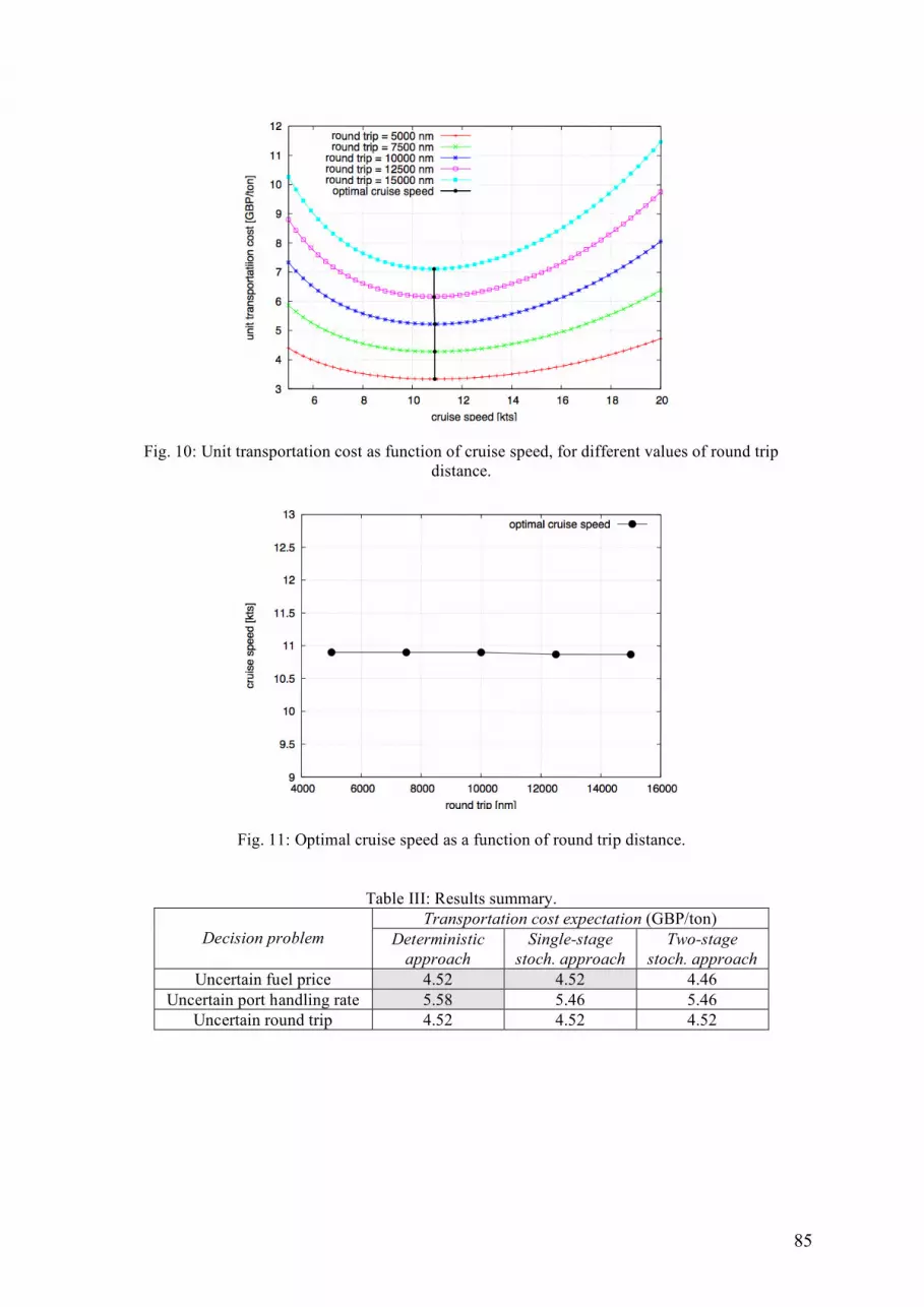
The last example shows the result of an optimization procedure aimed at minimum transportation cost when the round trip distance is an uncertain parameter. Again, a preliminary parametric analysis has been performed and the results are shown in Figs. 10 and 11. In this case as well, the optimal cruise speed does not vary with the round trip distance. Therefore, also in this case, the two-stage approach reduces to a standard single-stage stochastic approach. According to the fact that the dependence of the transportation cost on the round trip measure is linear, the latter procedure coincides with a standard deterministic optimization where the uncertain parameter is taken equal to its expectation. Figs. 12 and 13 confirm that, for the present problem, the three approaches coincide.

84

Fig. 8: Unit transportation cost as a function of port handling rate for optimal configurations.

Fig. 9: Non-dimensional first-stage variables for optimal configurations (uncertain port handling rate).

Table III summarized the above results in terms of transportation cost expectation, for the different optimization approaches. The results related to coincident approaches (as emerging in the specific cases considered) are displayed with the same background colour. As already pointed out, the advantage in approaching the design optimization as a two-stage decision problem, emerges in the uncertain-fuel-price case, with sensitive variation of the optimal second-stage decision with respect to the uncertain parameter. The two-stage stochastic approach reduces to a single-stage stochastic problem for the uncertain port-handling-rate case, in which no significant variation of the optimal second-stage decision is observed. When considering uncertain round trip, deterministic, single- and second-stage stochastic approaches all coincides, due to the fact that the second-stage optimal decision is constant with respect to the stochastic parameter and the dependence of the cost on the latter parameter is linear.

85

Fig. 10: Unit transportation cost as function of cruise speed, for different values of round trip distance.

Fig. 11: Optimal cruise speed as a function of round trip distance.

Table III: Results summary. Transportation cost expectation (GBP/ton)

Decision problem Deterministic approach

Single-stage stoch. approach

Two-stage stoch. approach

Uncertain fuel price 4.52 4.52 4.46 Uncertain port handling rate 5.58 5.46 5.46

Uncertain round trip 4.52 4.52 4.52

86

Fig. 12: Unit transportation cost as a function of round trip distance for optimal configurations.

Fig. 13: Non-dimensional first-stage variables for optimal configurations (uncertain round trip).

5. Concluding remarks A formulation for two-stage stochastic programming robust optimization of ship design has been presented and applied to the conceptual design of a bulk carrier under uncertain operating conditions. The numerical results confirm that the two-stage approach can be successfully exploited if the optimal second-stage decisions vary significantly upon uncertainty realizations. In this case, the present formulation gives lower values of the overall costs expectation. Some further remarks can be made in order to better clarify the impact of such an approach on the robust design optimization. The advantage in applying the two-stage stochastic paradigm is conditional on the dependence of the second-stage decision on the uncertainties variation. Specifically, the greater is the variation of the optimal second-stage decision with respect to the stochastic parameters variation, the greater is the advantage to approach the robust design optimization task as a two-stage stochastic programming problem. Conversely, if the optimal second-stage decision is constant with respect to the uncertainty realizations, then a standard single-stage stochastic approach is more convenient (because saving computational time).

87

Acknowledgements This work has been partially supported by the U.S. Office of Naval Research, NICOP grant no. N00014-08-1-0491, through Dr. Ki-Han Kim. References BEYER, H.G.; SENDHOFF, B. (2007), Robust optimization - a comprehensive survey, Computational Methods in Applied Mechanics and Engineering, 196 CAMPANA, E.F.; FASANO, G.; PERI, D.; PINTO, A. (2006), Particle Swarm Optimization: efficient globally convergent modifications, 3rd European Conf. on Computational Mechanics - Solids, Structures and Coupled Problems in Engineering, Lisbon. CAMPANA E.F.; LIUZZI G.; LUCIDI S.; PERI D.; PICCIALLI V.; PINTO A. (2009), New global optimization methods for ship design problems, Optimization and Engineering, 10 (4). DE GROOT, M.H. (1970), Optimal Statistical Decisions, McGraw Hill, New York. DIEZ, M.; PERI D. (2009), Global optimization algorithms for robust optimization in naval design, 8th Int. Conf. on Computer Applications and Information Technology in the Maritime Industries, (COMPIT), Budapest. DIEZ, M.; PERI D. (2010), Robust optimization for ship conceptual design, submitted to Ocean Engineering. KENNEDY, J; EBERHARD R., (1995), Particle Swarm Optimization, IEEE Int. Conf. on Neural Networks, Perth. PARK G.J.; LEE T.H.; WANG K.H. (2006), Robust Design: an overview, AIAA Journal, 44 (1). PARSONS, M.G.; SCOTT, R.L. (2004), Formulation of multicriterion design optimization problems for solution with scalar numerical optimization methods, J. Ship Research 48, pp.61-76. SAHINIDIS, N.V. (2004), Optimization under uncertainty: state-of-the-art and opportunities, Computers and Chemical Engineering 28, pp. 971-983. SEN, P.; YANG, J.B. (1998), Multiple Criteria Decision Support in Engineering Design, Springer, London. ZANG, C.; FRISWELL, M.I.; MOTTERSHEAD, J.E. (2005), A review of robust optimal design and its application in dynamics, Computers and Structures 83.

88

Appendix A: Bulk carrier conceptual design tool In this Appendix, the bulk carrier conceptual design tool used by Parsons and Scott (2004) is briefly recalled. In the present work, we extend the analysis, including a loan model in order to take into account the mortgage cost. Independent variables:

L = length [m] B = beam [m] D = depth [m] T = draft [m] CB = block coefficient Vk = cruise speed [knots] Vk,max = maximum cruise speed [knots]

Analysis tool:

capital costs = 0.2 ship cost ship cost = 1.3 (2,000 Ws0.85 + 3,500 Wo + 2,400 P0.8) steel weight = Ws = 0.034 L1.7 B0.7 D0.4 CB

0.5 outfit weight = Wo = L0.8 B0.6 D0.3 CB

0.1 machinery weight = Wm = 0.17 Pmax

0.9 displacement = 1.025 L B T CB power = P = displacement2/3 Vk

3/(a + b Fn) power max. = Pmax = displacement2/3 Vk,max

3/(a + b Fn) Froude number = Fn = V/(gL)0.5 Froude number max. = Fnmax = Vmax/(gL)0.5 V = 0.5144 Vk m/s Vmax = 0.5144 Vk,max m/s g = 9.8065 m/s2 a = 4,977.06 CB

2 - 8,105.61 CB + 4,456.51 b = - 10,847.2 CB

2 + 12,817 CB - 6,960.32 running costs = 40,000 DWT0.3 deadweight = DWT = displacement - light ship weight light ship weight = Ws + Wo + Wm voyage costs = (fuel cost + port cost) RTPA fuel cost = 1.05 daily consumption * sea days * fuel price daily consumption = 0.19 P 24/1,000 + 0.2 sea days = round trip miles/24 Vk round trip miles = 5,000 (nm) fuel price = 100 (£/t) port cost = 6.3 DWT0.8 round trips per year = RTPA = 350/(sea days + port days) port days = 2[(cargo deadweight/handling rate) + 0.5] cargo deadweight = DWT - fuel carried - miscellaneous DWT fuel carried = daily consumption (sea days + 5) miscellaneous DWT = 2.0 DWT0.5 handling rate = 8,000 (t/day) vertical center of buoyancy = KB = 0.53 T metacentric radius = BMT =(0.085 CB - 0.002) B2/(T CB) vertical center of gravity = KG = 1.0 + 0.52 D

89

Loan model:

loan = 0.8 ship cost rate of return = Rr = 0.100 rate of interest = Ri = 0.075 number of repayments per year = Py = 1 number of years = Ny = 20

annual repayment =

!

loan 1 + Ri/Py( )Py Ny

Ri/Py

1 + Ri/Py( )Py Ny

"1

net present value = capital cost +

!

voyage cost +running cost +annual repayment

1 + Rr( )k

k=1

Ny

"

annual transportation cost = net present value / Ny annual cargo capacity = DWT * RTPA unit transportation cost = annual transportation cost / annual cargo capacity

Constraints:

L/B ≥ 6 L/D ≤ 15 L/T ≤ 19 T ≤ 0.45 DWT0.31 T ≤ 0.7 D + 0.7 25,000 ≤ DWT ≤ 500,000 Fnmax ≤ 0.32 GMT = KB + BMT – KG ≥ 0.07 B Vk ≤ Vk,max