tutorial examine 2d - baixardoc

Quick Start Tutorial 1-1

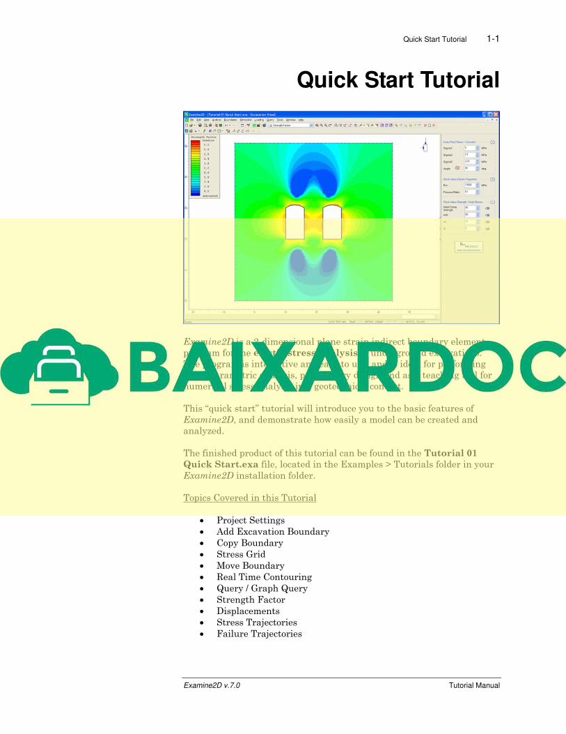
Quick Start Tutorial

Examine2D is a 2-dimensional plane strain indirect boundary element

program for the elastic stress analysis of underground excavations.

The program is interactive and easy to use, and is ideal for performing

quick parametric analysis, preliminary design and as a teaching tool for

numerical stress analysis in a geotechnical context.

This “quick start” tutorial will introduce you to the basic features of

Examine2D, and demonstrate how easily a model can be created and

analyzed.

The finished product of this tutorial can be found in the Tutorial 01

Quick Start.exa file, located in the Examples > Tutorials folder in your

Examine2D installation folder.

Topics Covered in this Tutorial

• Project Settings

• Add Excavation Boundary

• Copy Boundary

• Stress Grid

• Move Boundary

• Real Time Contouring

• Query / Graph Query

• Strength Factor

• Displacements

• Stress Trajectories

• Failure Trajectories

Examine2D v.7.0 Tutorial Manual


Introduction

Before launching into an analysis with Examine2D, it is important to

stop and consider the developmental philosophy of the program, the

assumptions inherent in the analysis and the resultant limitations.

Examine2D is designed to be a quick and simple-to-use parametric

analysis tool for investigating the influence of geometry and in-situ stress

variability on the stress changes in rock due to excavations. The induced

stresses in the plane of the analysis can be viewed by means of stress

contour patterns in the region surrounding the excavations. As a tool for

interpreting the amount of deviatoric overstress (principal stress

difference) around openings, strength factor contours give a quantitative

measure of (strength)/(induced stress) according to a user defined failure

criterion for the rock mass.

Some important limitations of the program which should be considered

when interpreting Examine2D output are described below.

The assumption of plane strain means that the modeled excavation is of

infinite length normal to the plane section of the analysis. In practice, as

the out-of-plane excavation length becomes less than five times the

largest cross-sectional dimension, the stress changes calculated by

Examine2D begin to show some exaggeration since the real stress flow

around the ‘ends’ of the excavation is not taken into account. All of the

stress is ‘forced’ to flow around the excavation parallel to the analysis

plane. This exaggeration becomes more pronounced as the out-of-plane

length approaches the same magnitude as the in-plane dimensions. As

long as this effect is kept in mind, the analysis may still yield useful

insight into behavioral trends in these cases.

The elastic boundary element analysis used in Examine2D dictates that

the material being modeled is assumed to be:

• homogenous

• isotropic or transversely isotropic

• linearly elastic

Obviously, most of the rock masses which will be modeled possess none of

these properties. The degree to which the actual rock mass being modeled

deviates from these assumed properties should be kept in mind when

interpreting Examine2D output. Nevertheless, the induced stresses

calculated and displayed by Examine2D can usually prove useful, for

example, when optimizing excavation geometry and/or sequencing to

avoid overstress and undesirable de-stressing.



The displacements shown by Examine2D are meant to qualitatively

illustrate regional deformation trends only. The actual values of the

displacements calculated by Examine2D include only the elastic

displacements due to the excavation. This, in reality, may constitute a

very small component of the actual measured displacements in the field.

In weak broken rock, the actual magnitude of displacements may be

several orders of magnitude greater than the calculated elastic values. In

addition, the calculated displacements depend directly on the value of the

Deformation (Young's) Modulus for the rock mass, a value difficult to

estimate.

The practice of performing multiple analysis runs using a range of stress

and material properties to study the effect of each parameter is a prudent

one in all cases.

In short, Examine2D is a powerful but, nevertheless, limited tool. Like all

numerical models, it should be used to enhance and supplement, but

never to replace, common sense and good engineering judgement.

New File

Start the Examine2D program by double-clicking on the Examine2D icon

in your installation folder. Or from the Start menu, select Programs →

Rocscience → Examine2D 7.0 → Examine2D.

If the Examine2D application window is not already maximized,

maximize it now, so that the full screen is available for viewing the

model.

Note that when Examine2D is started, a new blank document is already

opened, allowing you to begin creating a model immediately.



Project Settings

The Project Settings option is used to configure the main analysis

parameters for your model (e.g. Units, Field Stress Type, Strength

Criterion etc). Select Project Settings from the toolbar or the Analysis

menu.

Select: Analysis → Project Settings

You will see the Project Settings dialog.

Under the General tab in Project Settings, make sure the following

options are selected:

• Units = Metric, stress as MPa

• Field Stress Type = Constant

• Elastic Properties = Isotropic

• Strength Criterion = Generalized Hoek-Brown, with the Use

GSI, mi, D checkbox selected

Select the Analysis tab in Project Settings. We will use the default

options, which should be as follows:

• Number of Boundary Elements = 100



• Boundary Element Type = Constant

• Analysis Type = Plane Strain

• Matrix Solver Type = Jacobi Bi-Conjugate Gradient

Note: see the Examine2D Help topics for information about these options.

Select the Project Summary tab in Project Settings.

Enter Examine2D Quick Start Tutorial as the Project Title.

TIPS:

• The Project Summary information can be displayed on printouts

of analysis results, by using the Page Setup option in the File

menu and defining a Header and/or Footer.

• You can specify the Author and Company in the Preferences

dialog in the File menu, so that this information always appears

by default in the Project Summary in Project Settings, for new

files.

Select OK to close the Project Settings dialog, and save the selections you

have made.



Add Excavation Boundary

Now let’s add an Excavation Boundary. Select Add Excavation from the

toolbar or the Boundaries menu.

Select: Boundaries → Add Excavation

Enter the following coordinates in the prompt line at the bottom right of

the screen. Note: press Enter at the end of each line, to enter each

coordinate pair, or single letter text command (e.g. “a” for arc or “c” for

close).

Enter vertex [t=table,i=circle,esc=cancel]: 10 10

Enter vertex [...]: 16 10

Enter vertex [...]: 16 20

Enter vertex [...]: a

You will see the Arc Options dialog. Use Arc Definition Method = 3

points on arc, and set the Number of Segments = 8. Select OK. Now

you can enter the second and third points defining the arc.

Enter second arc point [u=undo,esc=cancel]: 13 21

Enter third arc point [...]: 10 20

Enter vertex [...]: c

By entering “c” at the last prompt, the boundary is automatically closed

(i.e. the last vertex is joined to the first vertex). Note that arcs in

Examine2D are actually made up of a series of straight line segments.

The Arc option and other useful shortcuts are also available in the right-

click menu, while you are defining a boundary.



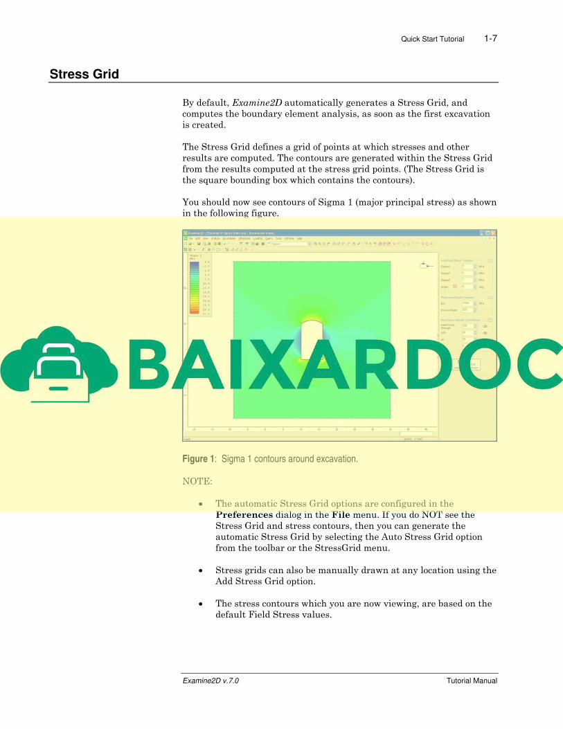
Stress Grid

By default, Examine2D automatically generates a Stress Grid, and

computes the boundary element analysis, as soon as the first excavation

is created.

The Stress Grid defines a grid of points at which stresses and other

results are computed. The contours are generated within the Stress Grid

from the results computed at the stress grid points. (The Stress Grid is

the square bounding box which contains the contours).

You should now see contours of Sigma 1 (major principal stress) as shown

in the following figure.

Figure 1: Sigma 1 contours around excavation.

NOTE:

• The automatic Stress Grid options are configured in the

Preferences dialog in the File menu. If you do NOT see the

Stress Grid and stress contours, then you can generate the

automatic Stress Grid by selecting the Auto Stress Grid option

from the toolbar or the StressGrid menu.

• Stress grids can also be manually drawn at any location using the

Add Stress Grid option.

• The stress contours which you are now viewing, are based on the

default Field Stress values.



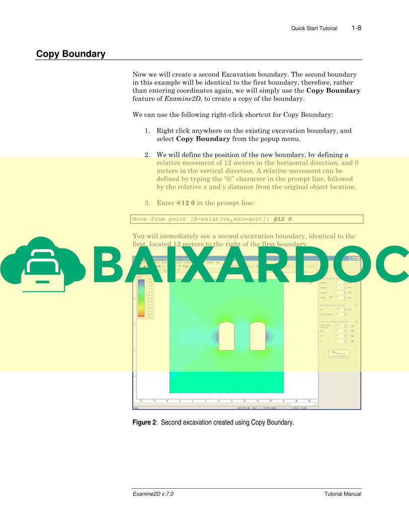
Copy Boundary

Now we will create a second Excavation boundary. The second boundary

in this example will be identical to the first boundary, therefore, rather

than entering coordinates again, we will simply use the Copy Boundary

feature of Examine2D, to create a copy of the boundary.

We can use the following right-click shortcut for Copy Boundary:

1. Right click anywhere on the existing excavation boundary, and

select Copy Boundary from the popup menu.

2. We will define the position of the new boundary, by defining a

relative movement of 12 meters in the horizontal direction, and 0

meters in the vertical direction. A relative movement can be

defined by typing the “@” character in the prompt line, followed

by the relative x and y distance from the original object location.

3. Enter @12 0 in the prompt line:

Move from point [@=relative,esc=quit]: @12 0

You will immediately see a second excavation boundary, identical to the

first, located 12 meters to the right of the first boundary.

Figure 2: Second excavation created using Copy Boundary.



Auto Stress Grid

Notice that the Stress Grid is NOT automatically re-generated, when you

add a new boundary. Therefore, let’s re-generate the Auto Stress Grid, so

that the two excavations are at the center of the contours.

Select: StressGrid → Auto Stress Grid

You will see the Grid Spacing dialog.

We will use the default spacing of 40 x 40, so just select OK in the dialog.

The Stress Grid and stress contours will be re-generated, and your screen

should appear as follows.

Figure 3: Stress grid re-generated using Auto Stress Grid.



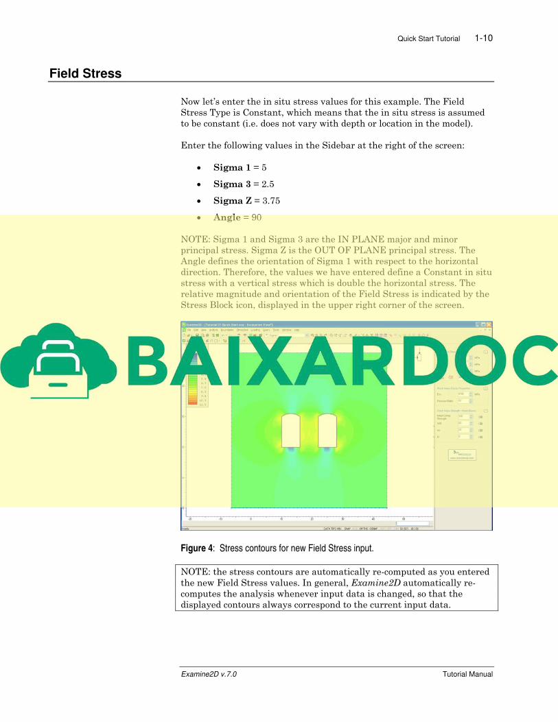
Field Stress

Now let’s enter the in situ stress values for this example. The Field

Stress Type is Constant, which means that the in situ stress is assumed

to be constant (i.e. does not vary with depth or location in the model).

Enter the following values in the Sidebar at the right of the screen:

• Sigma 1 = 5

• Sigma 3 = 2.5

• Sigma Z = 3.75

• Angle = 90

NOTE: Sigma 1 and Sigma 3 are the IN PLANE major and minor

principal stress. Sigma Z is the OUT OF PLANE principal stress. The

Angle defines the orientation of Sigma 1 with respect to the horizontal

direction. Therefore, the values we have entered define a Constant in situ

stress with a vertical stress which is double the horizontal stress. The

relative magnitude and orientation of the Field Stress is indicated by the

Stress Block icon, displayed in the upper right corner of the screen.

Figure 4: Stress contours for new Field Stress input.

NOTE: the stress contours are automatically re-computed as you entered

the new Field Stress values. In general, Examine2D automatically re-

computes the analysis whenever input data is changed, so that the

displayed contours always correspond to the current input data.


tutorial examine 2d - baixardoc

Documents