tuning status

Hendrik HoethLund University

Tuning Status

MCnet Meeting, Durham, 15 January 2009 1

Intro – for the new people in the room

Updates – what’s happened recently

Plans – where we are going

Overview

Overview MCnet Meeting, Durham, 15 January 2009 2

Physics Validation and Global Comparisons

Systematic global validation is essential when testing models ordeveloping general-purpose tunings.

Rivet is a validation/comparison framework for generators, basedon the HepMC event record. It is used to

• ensure that generators describe a wide range of data

• regression-test generators between releases

• provide input for tunings

Used by us and being introduced in ATLAS, maybe CMS . . . .

Introduction MCnet Meeting, Durham, 15 January 2009 3

RivetRivet is a library of tools (event shape calculators, jet algorithms,final state definitions, . . . ) and so far about 40 analysis routineswhich use them.

• Command line tools for running generators, analysing events,making comparison plots

• Histograms can be auto-booked from reference data files

• Observables are automatically cached

• User analyses loaded as plugins

• Reference data is included in the Rivet release

Documentation, download etc:http://projects.hepforge.org/rivet/


ProfessorProfessor is a tuning tool developed within MCnet.It extends the tuning strategy used by Delphi.

• Sample N random points in parameter spaceand run the generator with those settings

• For each bin of each distribution use the N MC runs to fit aninterpolation function in order to parametrise the MC output

• Construct overall χ2 comparing this parametrisation with dataand minimise

• Use different combinations of observables, weights etc. to get afeeling for stability, systematics . . .

http://projects.hepforge.org/professor/


Some Results – Pythia 6

First production tune, shown in Perugia: Pythia 6

• Flavour parameters tuned to LEP/SLD identified particlemultiplicity ratios (normalized to π±).

• Fragmentation, hadronization (Q2 and pT ordered showers)tuned to LEP event shapes, b-frag., multiplicities, momentumspectra

• UE/MPI (only with Q2 shower and old MPI model yet) tuned toTevatron data: minbias, Drell-Yan, jet correlations, . . .

We see many improvements. Even just the LEP tuning improvedthe agreement with Tevatron data!

Paper is mostly finished.

Updates MCnet Meeting, Durham, 15 January 2009 6

b

b b

b

b

b

b

b

b

b

DELPHIb

Pythia 6.418, Q2 new tune

Pythia 6.418, default

0

0.5

1

1.5

2

2.5

3

3.5b quark fragmentation function f (xweak

B )

0.1 0.2 0.3 0.4 0.5 0.6 0.7 0.8 0.9 1.0

0.6

0.8

1

1.2

1.4

f (xB)

MC

/d

ata

b bbbbbbb b bbbbbbb

b

b

b

b

b

b

b

DELPHIb

Pythia 6.418, Q2 new tune

Pythia 6.418, default

10−1

1

10 1

10 2

Scaled momentum, xp = |p|/|pbeam|

0 0.2 0.4 0.6 0.8 1

0.6

0.8

1

1.2

1.4

xp

MC

/d

ata

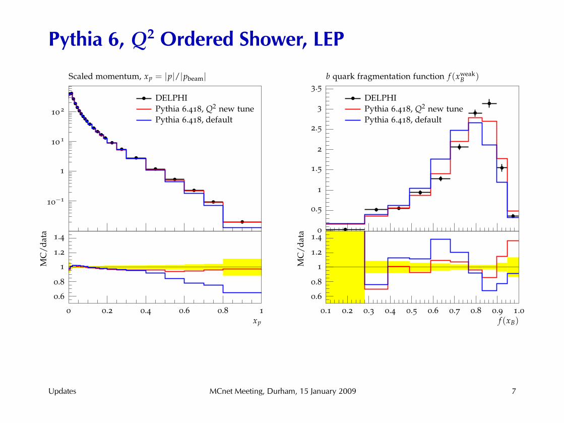
Pythia 6, Q2 Ordered Shower, LEP


b

DELPHIb

Pythia 6.418, pT new tune

Pythia 6.418, pT Λ = 0.23

Pythia 6.418, pT default

20.5

21

21.5

22

22.5

23

23.5

24Mean charged multiplicity

Nch

0.9

0.95

1.0

1.05

MC

/d

ata

b bbbbbbb b bbbbbbb

b

b

b

b

b

b

b

DELPHIb


Pythia 6.418, pT Λ = 0.23


10−1

1

10 1

10 2

Scaled momentum, xp = |p|/|pbeam| (charged)

0 0.2 0.4 0.6 0.8 1

0.6

0.8

1

1.2

1.4

xp

MC

/d

ata

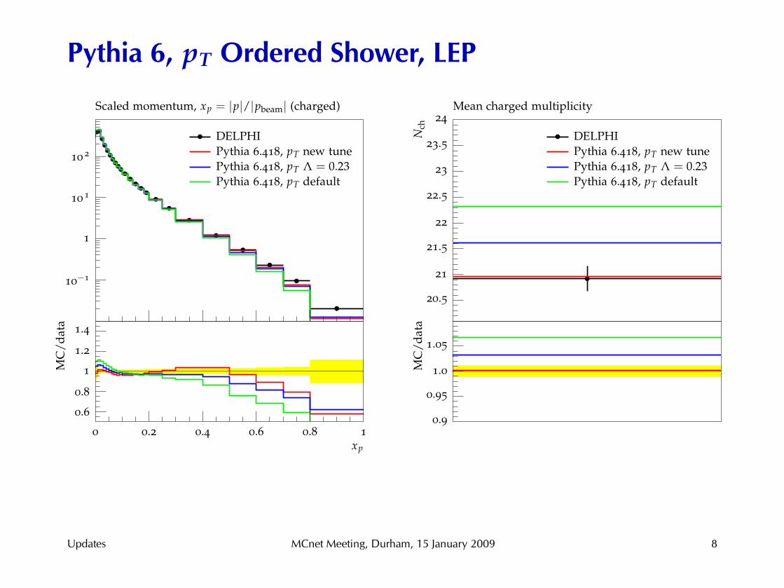
Pythia 6, pT Ordered Shower, LEP


b

b b bbbbbbbb

bb

bb

b

b

b

b

b

DELPHIb


Pythia 6.418, pT Λ = 0.23


10−2

10−1

1

10 1

1− Thrust

0 0.1 0.2 0.3 0.4 0.5

0.6

0.8

1

1.2

1.4

1− T

MC

/d

ata

b b b b b b b b b b bb

bb

b

b

b

b

b

b

b

DELPHIb


Pythia 6.418, pT Λ = 0.23

Pythia 6.418, pT default10−2

10−1

1

10 1

Rapidity w.r.t. Thrust axis

0 1 2 3 4 5 6

0.70.80.91.01.11.21.3

yT

MC

/d

ata

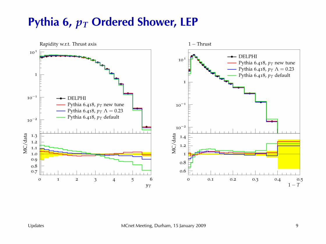
Pythia 6, pT Ordered Shower, LEP


bbbbbbbb b b b b b b b b b b b b b b b b b b b b b b b b b b b b b b

b bb

CDF Run-IIb

Pythia 6, new tune

Pythia 6, AW

0.7

0.8

0.9

1.0

1.1

1.2

1.3

1.4Mean track pT vs multiplicity – Minimum Bias

〈pT〉

5 10 15 20 25 30 35

0.8

0.9

1.0

1.1

1.2

Nch

MC

/d

ata

b

b

b

bb

b bb

bb

b b

b bb b

b

bb

bbb b b b

b

b bb b

bb b

b b b b b b b b b b b b b b b b b

CDF Run-Ib

Pythia 6, new tune

Pythia 6, AW

0

5

10

15

20

25

Z pT – Drell Yan

0 5 10 15 20

0.6

0.8

1

1.2

1.4

pT/GeV

MC

/d

ata

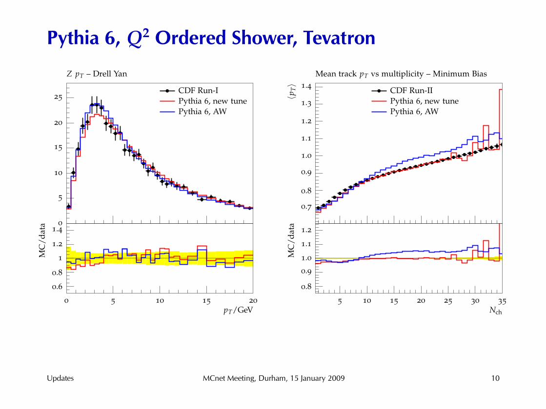
Pythia 6, Q2 Ordered Shower, Tevatron


b bbbb b

b b b b bb b b b b

bb b b

b b b

bb

b b

b b

b

CDF Run-IIb

Pythia 6, new tune

Pythia 6, AW

1

1.5

2

2.5

〈pT〉 versus Nch – Drell Yan

〈pT〉/

GeV

5 10 15 20 25 30

0.6

0.8

1

1.2

1.4

Nch

MC

/d

ata

b

b

b

b b bbb b b b b

b b b bb b b b

b b b b b bb

bb b b

bb

b

CDF Run-IIb

Pythia 6, new tune

Pythia 6, AW

0

0.2

0.4

0.6

0.8

1

Transverse Particle Density – Leading Jet Analysis

0 50 100 150 200 250 300 350 400

0.6

0.8

1

1.2

1.4

pT(jet 1)

MC

/d

ata

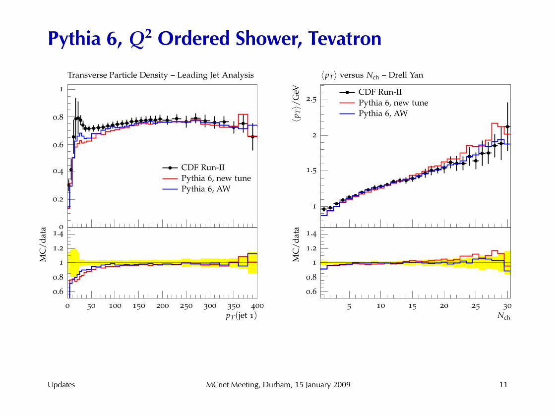
Pythia 6, Q2 Ordered Shower, Tevatron


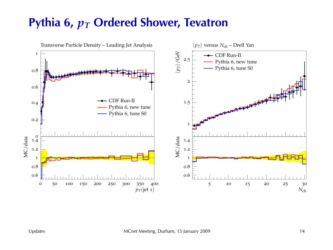
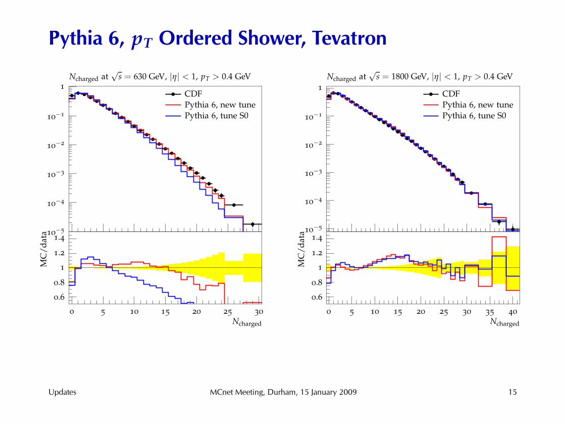
Hot of the Presses – Pythia 6

Tuning of the Pythia 6 pT ordered shower and new MPI model toTevatron data.

Will be finalized next week (Professor collaboration meeting inLund).

More data available for this tune than for the Q2 ordered tune –the Rivet development is always ongoing and largely driven by thetuning necessities.

Here’s a first peek on the results . . .


bbbbbbbb b b b b b b b b b b b b b b b b b b b b b b b b b b b b b b

b bb

CDF Run-IIb

Pythia 6, new tune

Pythia 6, tune S0

0.7

0.8

0.9

1.0

1.1

1.2

1.3

1.4Mean track pT vs multiplicity – Minimum Bias

〈pT〉

5 10 15 20 25 30 35

0.8

0.9

1.0

1.1

1.2

Nch

MC

/d

ata

b

b

b

bb

b bb

bb

b b

b bb b

b

bb

b

bb b b b

b

b bb b

bb b

b b b b b b b b b b b b b b b b b

CDF Run-Ib

Pythia 6, new tune

Pythia 6, tune S0

0

5

10

15

20

25

Z pT – Drell Yan

0 5 10 15 20

0.6

0.8

1

1.2

1.4

pT/GeV

MC

/d

ata

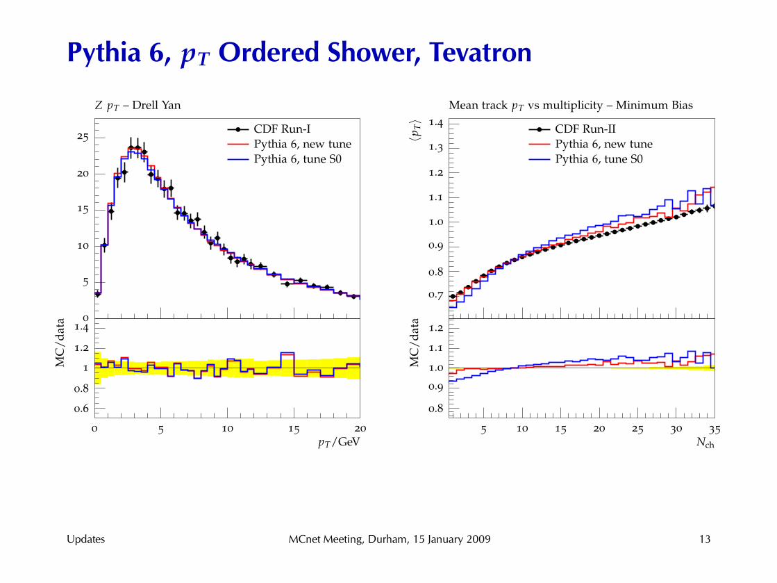
Pythia 6, pT Ordered Shower, Tevatron


b bbbb b

b b b b bb b b b b

bb b b

b b b

bb

b b

b b

b

CDF Run-IIb

Pythia 6, new tune

Pythia 6, tune S0

1

1.5

2

2.5

〈pT〉 versus Nch – Drell Yan

〈pT〉/

GeV

5 10 15 20 25 30

0.6

0.8

1

1.2

1.4

Nch

MC

/d

ata

b

b

b

b b bbb b b b b

b b b bb b b b

b b b b b bb

bb b b

bb

b

CDF Run-IIb

Pythia 6, new tune

Pythia 6, tune S0

0

0.2

0.4

0.6

0.8

1

Transverse Particle Density – Leading Jet Analysis

0 50 100 150 200 250 300 350 400

0.6

0.8

1

1.2

1.4

pT(jet 1)

MC

/d

ata



bb b b

bbbbbbbbbbbbbbbbbbbbbbbbbb

b

b

b

b

CDFb

Pythia 6, new tune

Pythia 6, tune S0

10−5

10−4

10−3

10−2

10−1

1Ncharged at

√s = 1800 GeV, |η| < 1, pT > 0.4 GeV

0 5 10 15 20 25 30 35 40

0.6

0.8

1

1.2

1.4

Ncharged

MC

/d

ata

b b bbbbbbbbbbbbbbbbbbbbb

bb

b

b

CDFb

Pythia 6, new tune

Pythia 6, tune S0

10−5

10−4

10−3

10−2

10−1

1Ncharged at

√s = 630 GeV, |η| < 1, pT > 0.4 GeV

0 5 10 15 20 25 30

0.6

0.8

1

1.2

1.4

Ncharged

MC

/d

ata



Summary and Outlook

• Pythia 6 successfully tuned (well, next week)

• Publications in progress

• Machinery works mostly smooth now

• Lots of additions/improvements in Rivet

• Coarse tune of what-will-be Sherpa-2.2 initiated

• Pythia 8 and Herwig in the queue

Summary and Outlook MCnet Meeting, Durham, 15 January 2009 16

Backup Slides

Backup Slides MCnet Meeting, Durham, 15 January 2009 17

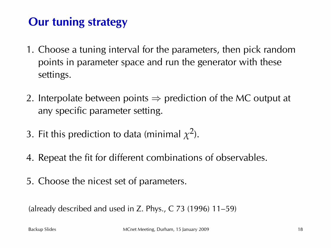
Our tuning strategy

1. Choose a tuning interval for the parameters, then pick randompoints in parameter space and run the generator with thesesettings.

2. Interpolate between points⇒ prediction of the MC output atany specific parameter setting.

3. Fit this prediction to data (minimal χ2).

4. Repeat the fit for different combinations of observables.

5. Choose the nicest set of parameters.

(already described and used in Z. Phys., C 73 (1996) 11–59)


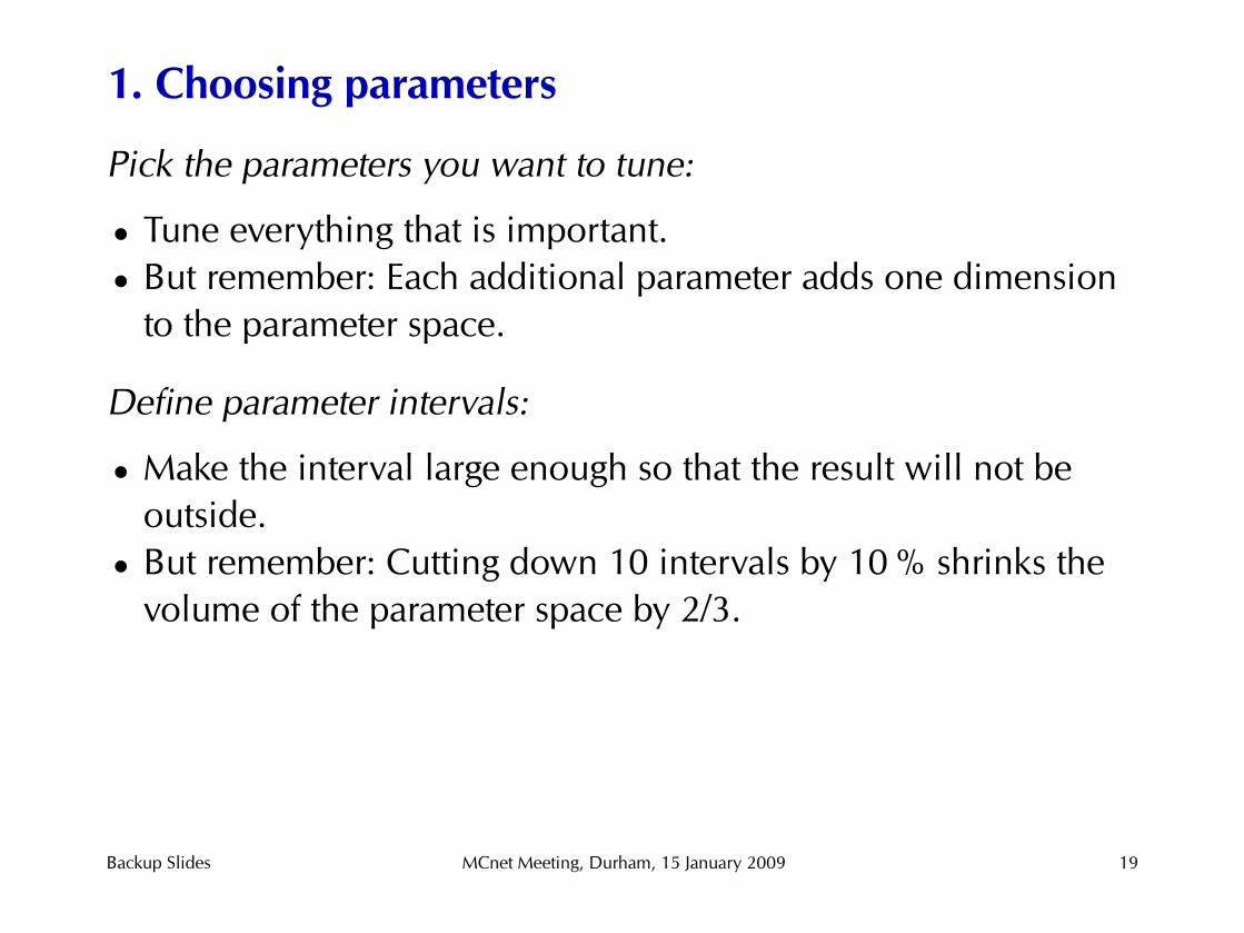
1. Choosing parameters

Pick the parameters you want to tune:

• Tune everything that is important.• But remember: Each additional parameter adds one dimension

to the parameter space.

Define parameter intervals:

• Make the interval large enough so that the result will not beoutside.• But remember: Cutting down 10 intervals by 10 % shrinks the

volume of the parameter space by 2/3.


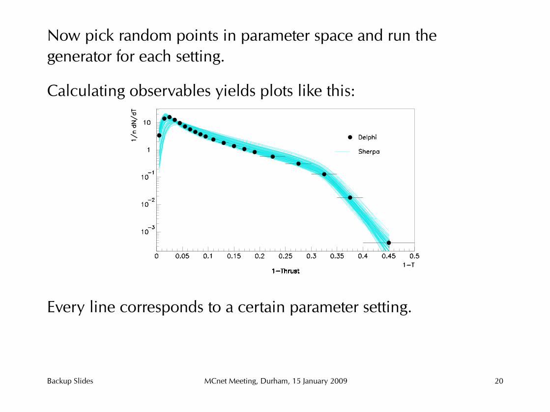
Now pick random points in parameter space and run thegenerator for each setting.

Calculating observables yields plots like this:

Every line corresponds to a certain parameter setting.


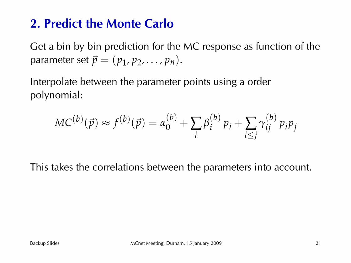
2. Predict the Monte Carlo

Get a bin by bin prediction for the MC response as function of theparameter set ~p = (p1, p2, . . . , pn).

Interpolate between the parameter points using a orderpolynomial:

MC(b)(~p) ≈ f (b)(~p) = α(b)0 + ∑

iβ(b)i pi + ∑

i≤jγ

(b)ij pipj

This takes the correlations between the parameters into account.


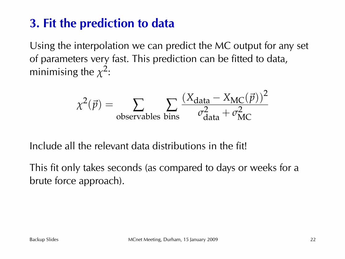
3. Fit the prediction to data

Using the interpolation we can predict the MC output for any setof parameters very fast. This prediction can be fitted to data,minimising the χ2:

χ2(~p) = ∑observables

∑bins

(Xdata− XMC(~p))2

σ2data + σ2

MC

Include all the relevant data distributions in the fit!

This fit only takes seconds (as compared to days or weeks for abrute force approach).


4.+5. Use different data sets, pick nicest tune

Now we approach the artistic part:

• Use different combinations of observables.

• Put different weights on the observables.

• Learn something about correlations and stability of the tuning.

• Interpret the results in the model’s context.

• Maybe adjust / fix parameters by hand.

• Pick the nicest result.


0.1 0.5 0.910 0

10 1

χ2/N

df

p̃

quadratic interpolation(s)

scan MC datamin(χ2/Ndf) = 3.9

10

40

∆N

∆p̃

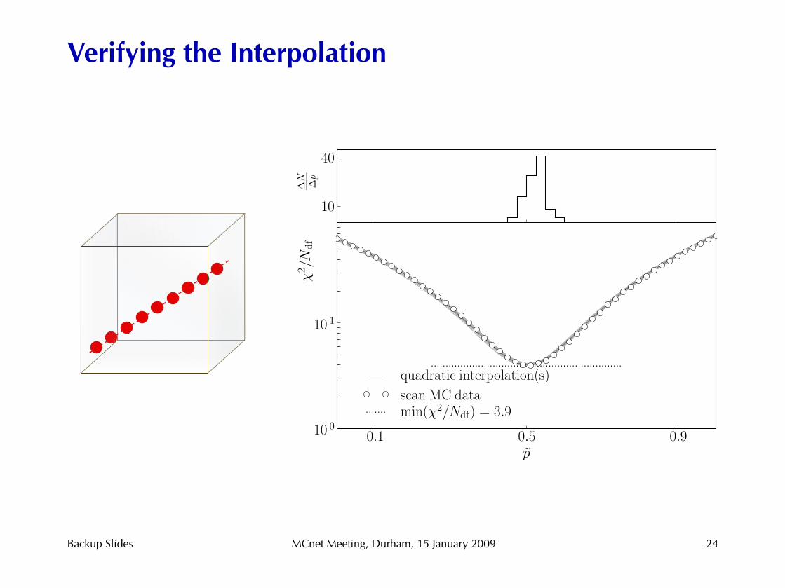
Verifying the Interpolation


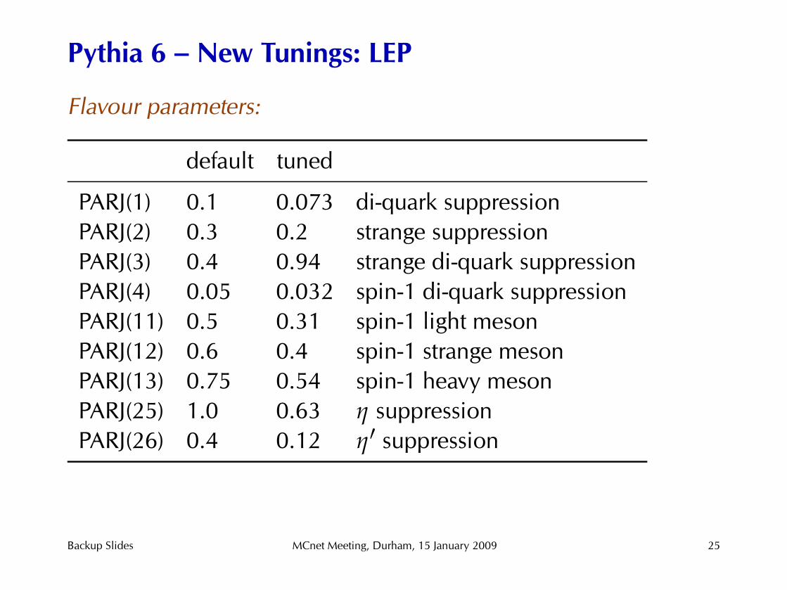
Flavour parameters:

default tuned

PARJ(1) 0.1 0.073 di-quark suppressionPARJ(2) 0.3 0.2 strange suppressionPARJ(3) 0.4 0.94 strange di-quark suppressionPARJ(4) 0.05 0.032 spin-1 di-quark suppressionPARJ(11) 0.5 0.31 spin-1 light mesonPARJ(12) 0.6 0.4 spin-1 strange mesonPARJ(13) 0.75 0.54 spin-1 heavy mesonPARJ(25) 1.0 0.63 η suppressionPARJ(26) 0.4 0.12 η′ suppression

Pythia 6 – New Tunings: LEP


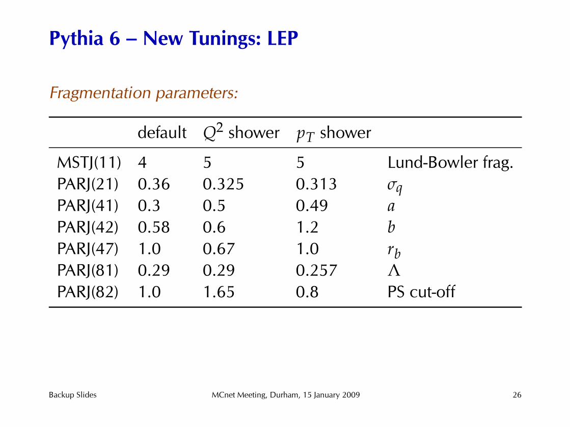
Fragmentation parameters:

default Q2 shower pT shower

MSTJ(11) 4 5 5 Lund-Bowler frag.PARJ(21) 0.36 0.325 0.313 σqPARJ(41) 0.3 0.5 0.49 aPARJ(42) 0.58 0.6 1.2 bPARJ(47) 1.0 0.67 1.0 rbPARJ(81) 0.29 0.29 0.257 ΛPARJ(82) 1.0 1.65 0.8 PS cut-off

Pythia 6 – New Tunings: LEP


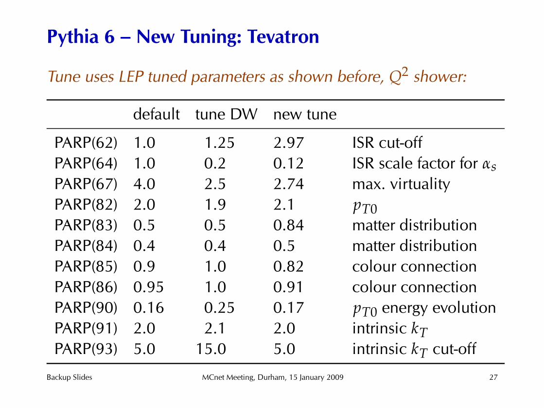
Tune uses LEP tuned parameters as shown before, Q2 shower:

default tune DW new tune

PARP(62) 1.0 1.25 2.97 ISR cut-offPARP(64) 1.0 0.2 0.12 ISR scale factor for αsPARP(67) 4.0 2.5 2.74 max. virtualityPARP(82) 2.0 1.9 2.1 pT0PARP(83) 0.5 0.5 0.84 matter distributionPARP(84) 0.4 0.4 0.5 matter distributionPARP(85) 0.9 1.0 0.82 colour connectionPARP(86) 0.95 1.0 0.91 colour connectionPARP(90) 0.16 0.25 0.17 pT0 energy evolutionPARP(91) 2.0 2.1 2.0 intrinsic kTPARP(93) 5.0 15.0 5.0 intrinsic kT cut-off

Pythia 6 – New Tuning: Tevatron


tuning status

Documents