automatic tuning algorithms for active filters

448 IEEE TRANSACTIONS ON CIRCUITS AND SYSTEMS, VOL. CAS-29, NO. 7, JULY 1982

Automatic Tuning Algorithms for Active Filters

DALE E. HOCEVAR, STUDENT MEMBER, IEEE, AND TIMOTHY N. TRICK, FELLOW, IEEE

Abstract-To meet filter response specifications active filters usually must be tuned or adjusted, preferably by computer automation if the production level is high. In this paper, three generalized tuning algorithms which have appeared in recent literature are comparatively reviewed on the basis of their architecture, computational complexity, and effectiveness. Furthermore, a new method is presented for the tuning resistor and frequency selection problem, a problem relevant to all three methods. Two Monte Carlo simulation examples enhance the comparison and provide a demonstration.

I. INTRODUCTION

T HE THEORY of active filters has grown into an immense body of knowledge encompassing many

aspects of synthesis, analysis, and design. These filters have found their place in many system realizations, usually in the form of hybrid integrated circuits. However, one of the practical problems in manufacturing such filters is that of achieving the desired response in view of random component variations and parasitic effects. The tuning problem is concerned with devising algorithms to correct for this by adjusting the components after production. Complicating the issue are the complex nonlinear equations involved; the need for efficient, computer implementable routines; and the restriction that only a subset of the components are adjustable. In particular it is usually only possible to trim the resistors and only in an irreversible, increasing manner.

In the past many methods have been devised for tuning active filters [ l]-[ 131 and these can be categorized as functional methods, deterministic methods, or as combinations of the two. Functional tuning means adjusting the components while applying an excitation to the circuit, on the other hand, deterministic tuning means analytically computing the necessary adjustments from a set of parameter measurements. Some of the deterministic methods [7]-[ lo] approach the problem with more mathematical and computational generality so that they can handle higher order filters and model parasitic and nonideal effects, and they require minimal preproduction effort for different filter types.

The intent of this paper is fourfold. The first is for this paper to be somewhat tutorial by incorporating compre- hensive reviews of two general automatic tuning methods [7]-[lo] and also by presenting comparative discussions.

Manuscript received June 22, 1981; revised February 11, 1981. This work was suouorted by the National Science Fomidation under Grant ENG 78-l 17% -

The authors are with the Department of Electrical Engineering and the Coordinated Science Laboratory, University of Illinois, Urbana, IL 6 1801.

The second intention is to present a new tuning method [ Ill, [ 121 which utilizes large-change-sensitivity information. The discussion is broadened by a section on the computational complexity of the algorithms. The third intention is to present and theoretically justify a new method for the selection and ordering of tuning resistors and frequencies. This selection problem is relevant to each tuning method, although manifested differently in each method. Lastly, new results from statistical simulations of the tuning process will be presented which will provide a comparison and demonstration of the practical effectiveness of these tuning methods on a common simulation basis.

II. DISCUSSION OF METHODS

In this section the three methods are presented and discussed in mutual setting. For more details and background the reader can see the references for the original presentations. The active filter circuits of interest can be described by their transfer function f(w,u, b) where w is a radian frequency, (I is the vector of tuning resistors, and b is the vector of remaining components. The general tuning problem is to find Au such that

f(.,a,+A~,b~+Ab)=f(.,u,,bo) 0)

where u0 and b,, are nominal values and Ab is the unde- sired but measurable change in the untuned components. However, since f is a rational function in o whose coefficients are algebraic functions of u and 6, equality above is guaranteed if it holds for a particular finite number of frequencies. The methods that follow can be interpreted as techniques for solving this equation at a finite number of frequencies.

A. Least Squares Method The least squares method is due to Antreich et al. [7], [8].

Let the general response function

F: R’XR’+R” (2)

F(u,b)=[F,(w,,u,b),-.,Fn(w,,a,b)]T (3)

be composed of n real valued response functions I;;’ at q different frequencies with w, u, and b the same as before. Logical choices for the functions 4 are the real and imaginary parts of the transfer function or the magnitude and/or

0098-4094/82/0700-0448$00.75 01982 IEEE

HOCEVAR AND TRICK: AUTOMATIC TUNING ALGORITHMS 449

phase of the transfer function. Denote the Jacobian of F as as an optimal control problem which was to m inimize

s = [s, :sb] (4) which is computed at the nominal values a0 and 6,. In the i=l

tuning procedure the response F(u,, 6, + Ab) is computed’ subject to at the q frequencies and the error vector Xk+l=Xk+hkUk (9b)

c=F(u,,b,+Ab)-F(u,,‘b,,) (5)

is calculated. It is desired to find a correction Au to be made to the tuning resistors which will m inimize the error E. This is formulated as

tin IIf’(x, 4, + Ab)- F(a,, &,)I], (6) x which can be identified as a nonlinear least squares problem [15]. One procedure for solving this problem is the Gauss-Newton method [ 161. The quantity within the norm is lineaiized and the resulting linear least squares problem is solved. Additional iterationi may be used in an attempt to further reduce the error. Antreich uses a simplification of this method. On ly the nominal point derivatives are used so that the solution or tuning element correction vector can be computed as

Au- -[S$S=]-‘S:e= -Sic. (7)

Here SJ is the pseudoinverse’ of S, and can be precom- puted and stored. The actual tuning procedure is to compute E from (5) and then to compute the nece?sary Adjustment from (7). If F is sufficiently linear with respect to the tuning resistor vector a, this method should work well. Antreich used one iteration of this procedure in his example, but suggested using more if necessary. However, one should proceed cautiously since nominal point derivatives are used and the iterates may not converge.

B. Sequential Tuning Algorithm The second method is called sequential tuning and was

proposed by Lopresti [9], [lo]. Let F be as before and define the quantities

1 @a) 3F

hk = GkaG, @b)

Here the Ci’s are capacitances; the Gci’s are shunt conductances across the capacitors which mode l dissipation effects of the capacitors. The nominal values of these conductances are usually assumed to be zero; the G ,‘s are the tuning conductances; furthermore, all derivatives above are computed at the nominal value. Lopresti cast the problem

Xl =x,7 k=l;..,r (94 where x,+, = dF, the differential of F. The yi’s must be positive and are usually chosen as lo-“; Q must be positive semidefinite and is usually chosen to be diagonal in such a way to have a normalizing effect. The solution to this quadratic problem is given as

uk =Hkxk, k=l;..,r 00) where the sequence of row vectors Hk are given in closed form in terms of the known parameters and are computed and stored in the preproduction stage. Hence, the algorithm is to measure the .components and compute xc, and then sequentially compute the uk’s. The best results are achieved if the resistor corresponding to ui is adjusted, then measured, and then the measured value is used to compute the actual achieved tii, which is then used to compute the new xi+,. This improvement is because there is always trimming error and this procedure uses that extra feedback beneficially. One can also choose F to be the vector of transfer function coefficients as was the case in the original presentation [9].

C. The Large-Change-Sensitivity Method A new large-change-sensitivity method was recently pro-

posed by Alajajian and Trick [ 111, [ 121. The foundation of the derivation is the differential form of Tel legen’s theorem, which is

i (AVklkik-AIkfk)= - i (AV,i,j-Alp,~~). k=l j=1

01) The terms on the right-hand side of (11) represent independent source branch voltages and currents including output port branch constraints, while the voltages and currents on the left-hand side of the equation represent the remaining branch constraints. Equation (11) was derived under the assumption that there are three topologically identical networks, N, N, and NA. The component values in the NA network have been perturbed from those in N such that the voltages and currents in the NA network are V, + AV,, and Ik + AI,, respectively. Equation (11) relates changes in voltages and currents in the N network to the voltages and currents in the fi network.

Next we consider the branch constraints. The conduc- tance branch constraints in the manufactured network N are

Ik = GkVk (12)

’ The response can also be measured, al though the following discussion and in the tuned network N,

must be altered slightly. Ik + AIk = (G, + AG,)(V, + AV,). (13)


Subtracting (12) from (13) gives AIk=G,AVk+GG,(Vk+AVk). (14)

If the branch constraints of l’? are chosen such that fi is the adjoint circuit of the network N, for example,

ik = Gkfk (15) then the substitution of these adjoint network branch constraints and the differential branch constraints into (11) give

k=l j=l

(16)

where r is the number of tuning elements and where a single input port and a single output port is assumed on the right-hand side of (16). Let port 1 denote the input port and port 2 denote the output port, and assume that the input port has a voltage source connected across its termi- nal pair. Since the purpose of tuning is to correct for deviations in response at the output port (to within a constant), the quantities of interest are the output voltage I$, or its change AV,. On this basis, choose pP, = 0 V and

Ip2 = 1 A so that (16) becomes

i (V-k+AVk)fkAGk=Av,,. 07) k=l

Requiring the output voltage of the tuned filter to be within a constant of the nominal value over the frequency spectrum results in

where V,, and V,, are the output voltages of the manufactured and nominal design circuits, respectively, the super- script j denotes the frequency at which the deviation is computed, and c is an unknown constant. Let q represent the number of critical frequencies at which the measurements are made. Then (17) becomes

Y” (4 (214

where a is the vector of tuning conductances. The key to the large-change-sensitivity method is a different assumption about the AV’s which works much better than the Newton step. Since the tuned circuit will have essentially the same poles as the nominal circuit, and the zeros of the transfer functions for the internal branches will typically lie outside of the passband of the filter, the branch voltages in the tuned circuit may be approximated as

(V, + AV,)‘= V,, (22)

where the vkd’s are nominal circuit branch voltages. Hence the tuning method becomes an iterative algorithm where in each iteration the adjoint and manufactured voltages are computed and the solution update AG ‘s are computed from (19).* Convergence can be checked at each iteration by stopping when the voltages on the right-hand side of (19) are within specified tolerances of their nominal values. Usually only one to three iterations are necessary with the greatest improvement occurring in the first step.

Some similarities and differences between these methods can be seen more easily now. The least squares and large- change-sensitivity methods are similar in that they can be viewed as direct methods for solving a nonlinear equation. In particular, the least squares method uses the Gauss- Newton method with nominal point derivatives for solving the problem in a least squares fashion. The large-change- sensitivity method employs the Newton method with a so called large-change Jacobian instead of the standard Jacobian and this enhances its performance. The major computational difference between these two methods is that the large-change-sensitivity method updates its solution matrix while this matrix is kept constant in the least squares method. This large-change Jacobian could also be used to replace the Jacobian in the least squares method to

(V,+AV,)‘f,’ .a. (v,+Av,)‘~’

(19)

In order to linearize this equation one must make an assumption about the AV’s. If they are neglected the consequence is that

and the result is a Newton step for solving the equation

G(y)=0 (214

G(Y) A [v,t~,~,),...~~(~,~q,]T

-#&Q>,*-- Y v,,(~,>] * W-J)

produce a quickly convergent algorithm which would be able to use more frequencies than the large-change-sensitivity method. Another point to be made about the least squares and large-change-sensitivity methods is that they both require matrix inversions and can only use a subset of the resistors. Hence a resistor selection procedure is necessary for these two methods. The least squares and sequential methods both minimize a weighted sum of squares of

2Since the AC’s and c are real this equation is solved by decomposing each row into real and imaginary parts which allows one to use approxi- mately one-half as many frequencies as tuning resistors.


the error and linearize nonlinearities with nominal point derivatives. Both also represent an application of known numerical techniques to the problem while the large- change-sensitivity method uses a circuit theoretic approach to derive the large-change Jacobian. All three methods do attempt to solve (1) at a set of discrete frequency points.

III. TUNINGRESISTORAND FREQUENCYSELECTION

A fundamental requirement common to all the algorithms is a tuning resistor and frequency selection procedure which insures good performance of the algorithm. The performance is directly related to this choice, and it is not immediately obvious how to make this selection when considering the interplay between the different facets involved. For example, our experience [14] has shown that for many well reasoned choices of tuning resistors, the least squares and large-change-sensitivity algorithms did not converge, or the convergence was very poor in that many iterations were necessary or negative element values were generated. In our work we have found that the resistor selection problem is more critical than the frequency selection problem. These two problems are discussed separately below.

A. Tuning Resistor Choice Since the tuning methods are attempting to solve a

nonlinear equation, and since there is flexibility in the choice of parameters, it is logical to choose those individual parameters which have a strong effect on the function behavior. However, it is more reasonable to choose a set of parameters which as a group has a strong effect. This becomes clearer if one lets F be the function describing the equation and x the set of possible tuning parameters. For instance, let F be the composite function of the magn itude of the function in (1) taken at a set of frequency points. The linearization of F about x,, is

F(x)=F’(x,)(x-x,,)+F(x,). (23) Hence, the translated range space of F(x,) approximates the range space of Fin a small region about x,,, or in other words, the behavior of F’(x,) approximates the behavior of F ignoring translation. Observe that each component of x corresponds to a column of F’(x,) and that the number of resistors comprising x will almost always be larger than the rank of F’(x) regardless of the number of component functions in F. This is because F is composed of a rational function and typically the nature of RC active filters is such that the number of components exceeds the number of coefficients in the transfer function and obviously the maximum possible rank is the number of coefficients. Thus one can reason that it is desirable to determine a set of “strong” linearly independent columns of F’(xo) whose span approximates the span of F’(x,). These columns correspond to a set of resistors which should facilitate good movement in a region about F(x,).

Complementary to this concept is the following reason- ing. Observe that the least squares and large-change-sensi-

tivity methods involve the solution of a linear equation, hence the need arises to insure that the matrices are not ill condit ioned so that the algorithm will be numerically sta- ble. In the large-change-sensitivity method if one approximates the matrix in (19) by setting the AV ‘s to zero the matrix becomes a Jacobian. Hence, the desire to determine a set of strong linearly independent columns can also be interpreted as a means of insuring against ill conditioning of the particular matrices.

In the past others [l], [7], [8], [lo], and [13] have employed derivative information for the selection of tuning components, but their selection procedures do not neces- sarily lead to a well-conditioned set of columns. W e present a theoretical basis as well as a method which solves this problem in the following.

The subtending problem is: given a matrix determine a set of strong linearly independent columns within that matrix whose span approximates the span of the matrix. This is similar to the problem of rank degeneracy in linear least squares problems for which a useful technique has recently been developed [17]. The form of this technique that uses QR factorization with column pivoting was found to be effective in the problem at hand and the reasons for this are developed next; helpful background can be found in [ 17]-[20].

Every n X r matrix A, where, we assume that n 2 r throughout this section (without loss of generality), has r singular values which are arranged as

a,(A)k~,(A)a.. h,(A)>O. (24)

The rank of A is given by the index of the last nonzero singular value. More importantly there is a strong relation between the number of relatively large singular values and the number of strong linearly independent columns. For example, if A is a noisy version of another matrix of rank p < r then A will probably have rank r, but will have “strong” rank p, or p relatively large singular values. This is the concept of numerical rank which determines if A is close to another matrix of defective rank and provides tolerances for the degree of closeness. In [ 171 this is defined precisely and it is shown that the singular values can be used directly to determine the numerical rank and tolerances. The number of relatively large singular values can be used to estimate the number of tuning components to be used.

The QR factorization is used to order the components in such a fashion that the ones ordered first form an independent set. This factorization is of the form

A=QR (2%

and can always be computed where Q is orthogonal and R is upper triangular. If column pivoting is used (that is, interchanging the columns such that at every step the one being pivoted on has the largest norm) then the factorization is actually of the matrix a = AP where P is a square permutation matrix. The consequence of this is that for


a = QR, {rii} = R one has

rika Z r,:, Vj>k,k=l;..,r (26) i=l

1r111~132*1~~** al’rrl. (27) The reason for this lies in the column interchange and the special orthonormal properties of the matrix which premul- tiplies the factorization at each step in its computation. Recalling that R is zero below the diagonal, it is observed that a strong set of linearly independent columns are formed at the front of R. To see the importance of this, partition a = QR .as

1 (28) then

A1,Q,EIRnXk, R,,EUPk

A, =Q,R,, = [Q,rQzl ‘;’ . [ 1 (29)

The goal was to find a set of strong linearly independent columns of A and these usually can be found in A,, for the proper choice of k, because the singular values of A, and R,, are identical and because of (26) and (27).

One can also use the values Irii I to estimate the conditioning of A since in practice 1 rii I = a,( A). In fact, an upper and lower bound [20] can be given as

3(4’+6i - 1)-l’* Irii(Gai(A)G(r+i+l)“*[rii].

(30) However, of primary interest is the conditioning of A, (equivalently R, , ) which can be- determined from its largest and smallest singular values.3 Rather than compute these for several values of k they can be approximated by the diagonal elements of R , , ; using (30) one has the bounds

lr11l~~1~~,~~~~+2~“*1~11I (31) and

.3(4k +6k - 1)-l’* IrkkI~ok(A1)6(2k+1)“*~rkk~.

(32) Actually, in the numerous examples that have been done in this work the singular values have been computed at each step and were always found to be in close agreement with the values I rr: I.

The above discussion explains why the QR method works. It has been applied to numerous examples [14], mostly in conjunction with the large-change-sensitivity method. The results have shown that these selections con- sistently outperformed others that were tried. Furthermore, the best results were obtained when the particular matrices were row and column scaled in such a manner that the

3For a square matrix its condition number can be expressed as the first singular value divided by the last.

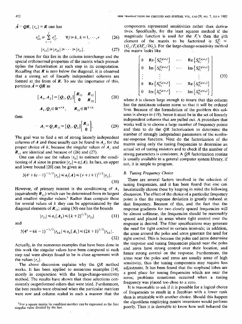
components represented sensitivities rather than derivatives. Specifically, for the least squares method if the magnitude function is used for the E;.‘s then the ijth element of the matrix to be factorized is S$ = ( Gj /&)( Cl& / aG,>. For the large-change-sensitivity method the matrix looks like

b Re{Sz(“l)} ... Re{$‘$“l)}

0 Im(s$(“I)) ... Im(s$(“I))

b Re(S$(“n)} ..+ Re(s:(“n)}

0 Im(~~cUn)] ..a Irn(Sz(-n))

(33)

where b is chosen large enough to insure that this column has the maximum column norm so that it will be ordered first. Because of the formulation of the problem this column is always in (19), hence it must be in the set of linearly independent columns that are pulled out. A procedure that works well is to choose a large number of frequency points and then to do the QR factorization to determine the number of strongly independent parameters of the nonlinear-response function. Next do the factorization of the matrix using only the tuning frequencies to determine an actual set of tuning resistors and to check if the number of strong parameters is consistent. A QR factorization routine is usually available in a general computer system library, if not, it is simple to program.

B. Tuning Frequency Choice There are several factors involved in the selection of

tuning frequencies, and it has been found that one can heuristically choose these by keeping in mind the following discussion. The effect of the choice of a particular frequency point is that the response deviation is greatly reduced at that frequency. Because of this, and the fact that the response gradients for two closely spaced frequencies will be almost collinear, the frequencies should be reasonably spaced and placed in areas where tight control over the response is desired. The filter specifications may generate the need for tight control in certain intervals; in addition, the areas around the poles and zeros generate the need for tight control. This is because the poles and zeros determine the response and tuning frequencies placed near the poles and zeros have strong control over their location, and hence strong control on the response. Furthermore, the areas near the poles and zeros are usually areas of high sensitivity, thus the tuning components may require less adjustment. It has been found that the stopband lobes are a good place for tuning frequencies which are near the zeros; problems sometimes occurred when a tuning frequency was placed too close to a zero.

It is reasonable to ask if it is possible for a logical choice of frequencies to result in a Jacobian with a lower rank than is attainable with another choice. Should this happen the algorithms employing matrix inversions would perform poorly. Thus it is desirable to know how well behaved the


rank of the particular Jacobian is with respect to the choice of frequencies. The Appendix discusses this issue and presents results which indicate that the rank of the Jacobian is not defective for logical frequency choices.

To conclude, many examples [14] have shown that the use of these heuristic guidelines for frequency selection in conjunction with the QR factorization for tuning element selection provide well-conditioned matrices for the algorithms and yield excellent results. At this point some comments about the number of tuning frequency points are in order. For the least squares method using magn itude functions the number of frequencies must be greater than or equal to the number of tuning resistors if the function is set up as in [7] because S,‘s, must be nonsingular in (7). One chooses only as many as are necessary because of the increased computational complexity. The large-change- sensitivity method requires that the number of frequencies be equal to r/2 or (r + 1)/2 where r is the number of tuning resistors. For the sequential method there is no real restriction other than the final performance, so one selects as few as will provide good results.

IV. COMPUTATIONALCOMPARISON

In this section the computational requirements of the tuning methods are discussed. Keep in m ind that these algorithms are to operate on a small computer system within a computer-aided-manufacturing environment. The assumptions are made that resistor and capacitor values are known from measurement when needed and that re- sponses are then simulated not measured.

In the preproduction stage each method requires a different set up procedure for a particular filter, however the effort is about the same for each method. Derivative information and Monte Carlo simulations are necessary in this setup procedure, hence a circuit simulation routine is es- sential. The derivative information is used to compute the various matrices and vectors needed in the implemen- tations, also for choosing the tuning frequencies, and especially for selecting a subset of tuning resistors for the least squares and large-change-sensitivity methods. Much of this was discussed in Section III.

In the production stage the computational complexity is quite different for each method. The sequential tuning method requires only a few vector operations for each resistor; specifically, a vector inner product (10) to compute the tuning correction, a scalar by vector product and vector sum (9b) to update the differential approximation, and a few trivial operations. Also, initially for each manufactured circuit the linear combination of vectors in (8a) must be computed to get the initial differential approximation. The least squares method is more complex requiring a set of linear circuit simulations to get the response error vector (5), then a matrix by vector product (7) to compute the tuning correction vector for each iteration. F inally, to check circuit acceptability a final set of simulations or alternately a matrix by vector product [7] must be done. The large-change-sensitivity method is slightly more complex. The large-change Jacobian in (19) must be updated at

each iteration which requires a set of linear circuit simulations to determine the necessary voltages and some mu lti- plications as indicated within the matrix. Then the small set of linear equations in (19) must be solved in order to compute the tuning corrections. A final set of simulations is used to determine circuit acceptability.

In summary, the preproduction effort and necessary software is about the same for each method; however, the production effort is m inimal for the sequential tuning method, but greater for the least squares and large- change-sensitivity methods. This is relative though, in abso- lute terms the computational effort is not very great for any of the methods since the circuit simulations are simply sparse linear equations.

V. MONTE CARLO EXAMPLES

In the following, two Monte Carlo simulation examples are presented, but first the simulation set up procedures are discussed. The statistical and parasitic mode ling is as follows. The random parameter deviations that are used are all generated from triangular density functions. Trimming tolerances are specified separately for the tuning and non- tuning resistors. Capacitor dissipation effects are mode led using shunt conductances, and the dissipation factor is defined as d = I/oRC where we choose a m idband frequency for the computation. The density of d is centered at 0.002 with widths of % O .OOl. For,each manufactured circuit a 2 l-percent deviation is generated and random capacitor values are computed by adding this first deviation to a *Cpercent deviation generated for each capacitor. This amounts to a f5-percent tolerance with the capacitor tracking mode led for thin film hybrid circuits; actually the tracking effect is usually stronger. The simulation for the sequential method emp loyed the feedback of the actual random values of the previously tr immed resistors at each step. The other two methods assumed that the untuned resistors were tr immed to nominal within the specified tolerance and that these values were available for the simulation.

Example 1. This example is an elliptic fifth-order low- pass filter taken from [7] and shown in F ig. 1. The nominal response is shown in F ig. 2, while the tuning resistor and frequency information is given in Table I. The tuning resistors used for the least squares method are the same as specified in [7] and are almost the same as those specified by ‘our QR method. Transfer function magn itude was chosen to be the response function in (3). The tuning resistors for the large-change-sensitivity method came from the QR method. The resistor ordering for the sequential method was done as suggested in [lo]; that is, the response magn itude error was ordered from greatest to least at 3400 Hz when individual l-percent changes were made in the resistors. Again the response function was transfer function magn itude and the performance index (9a) was chosen exactly as for the example in [lo]. Capacitor dissipation was calculated at 3400 Hz.

For this example. 100 sample circuits were used and the trimming error for all resistors was set to 20.2 percent.

454 IEEE TRANSACTIONS O N CIRCUITS AND SYSTEMS,VOL. CAS-29,NO.7,JULY 1982

TABLE I TUNINGFREQUENCYAND RESISTORINFORMATION

Method Example 1 Example 2

tuning frequencies tuning resistors or tuning resistors or order tuning frequencies order

Least 1000, 2500, 3400, Squares 3600, 3800, 4000, 8,11,1,20,3,17

5500 (Hz) : Large- 1000, 3400, 4000, 980, 1000,

Change- 5500 (HZ) 8,11,17,12,4,20.3 1020 (Hz) 10,9,4,5,8 Sensitivity

1000, 2500, 3400, 985, 995, (full order) 9,12, 3600, 3800, 4000, 8,9,10,17,20,12,11 1005, 1015 (,HZ) 11,3,6,10,5,4,2,8,

Sequential 5500 (Hz) 1,4,18,19,5,3,13,15 1,15,16,7,17,14,13

(QR) 10,9,4,5,8

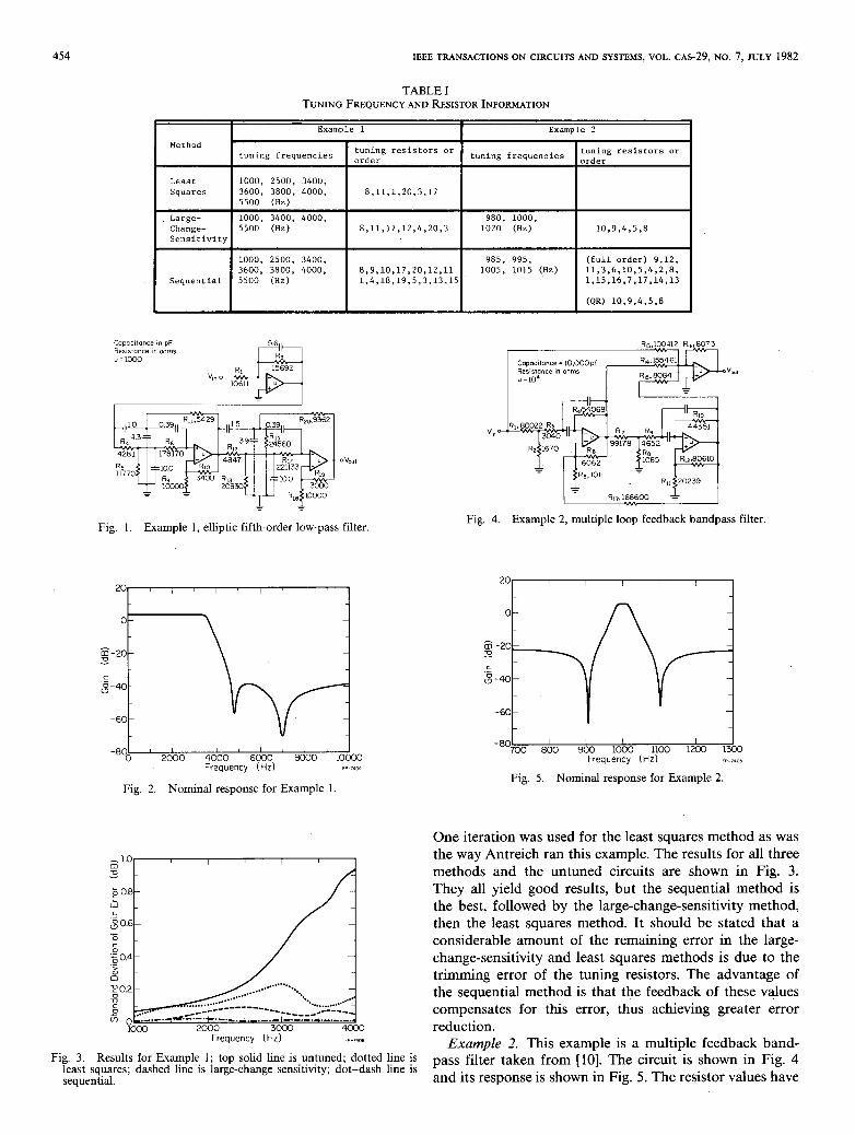
Fig. 1. Example 1, elliptic fifth-order low-pass filter.

-801 ’ ’ ’ 1 ’ 0 2000 4000 6000 8000 1oOxI Frequency (Hz) FP-,am

Fig. 2. Nominal response for Example 1

Frequency (Hz)

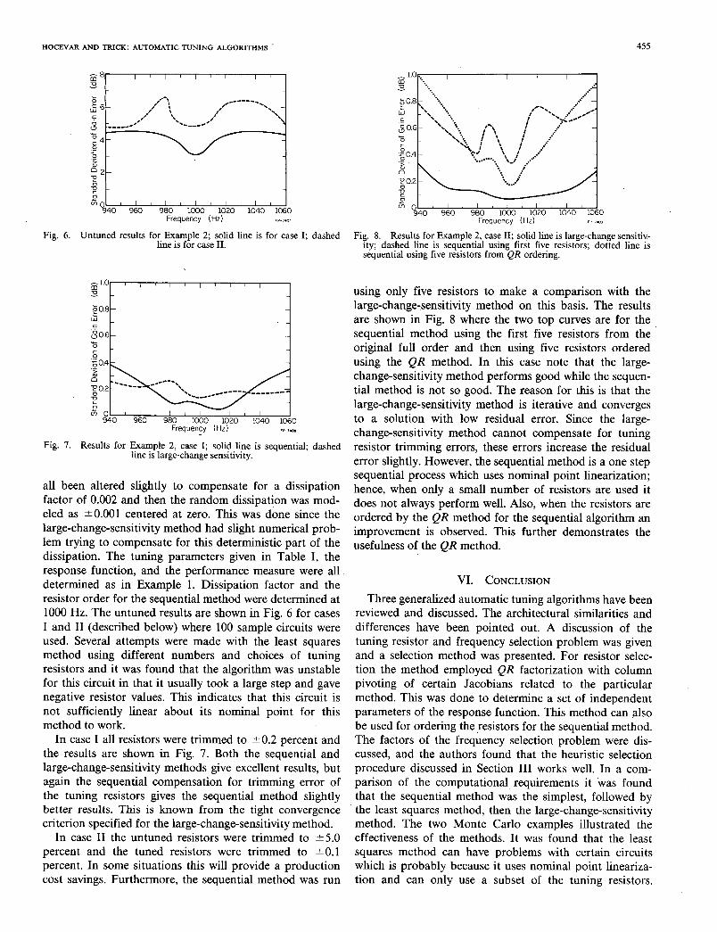
Fig. 3. Results for Example 1; top solid line is untuned; dotted line is least squares; dashed line is large-change sensitivity; dot-dash line is sequential.

Fig. 4. Example 2, multiple loop feedback bandpass filter.

-801 I / , I I I 700 800 900 1000 1100 1200 lx)0

Frequency (Hz) FP-iaos

Fig. 5. Nominal response for Example 2.

One iteration was used for the least squares method as was the way Antreich ran this example. The results for all three methods and the untuned circuits are shown in Fig. 3. They all yield good results, but the sequential method is the best, followed by the large-change-sensitivity method, then the least squares method. It should be stated that a considerable amount of the remaining error in the large- change-sensitivity and least squares methods is due to the trimming error of the tuning resistors. The advantage of the sequential method is that the feedback of these values compensates for this error, thus achieving greater error reduction.

Example 2. This example is a multiple feedback bandpass filter taken from [lo]. The circuit is shown in Fig. 4 and its response is shown in Fig. 5. The resistor values have

HOCEVAR AND TRICK: AUTOMATIC TUNING ALGORITHMS - 455

'"0 8 " " ' 4 " " 940 960 980 loo0 1020 1040 1060

Frequency (Hz) 10~1Ac3

Fig. 6. Untuned results for Example 2; solid line is for case I; dashed line is for case II.

Fig. 8. Results for Example 2, case II; solid line is large-change sensitivity; dashed line is sequential using first five resistors; dotted line is sequential using five resistors from QR ordering.

940 960 980 1000 1020 1040 1060 Frequency (Hz) re~,acE

Fig. 7. Results for Example 2, case I; solid line is sequential; dashed line is large-change sensitivity.

all been altered slightly to compensate for a dissipation factor of 0.002 and then the random dissipation was mod- eled as ?O.OOl centered at zero. This was done since the large-change-sensitivity method had slight numerical problem trying to compensate for this deterministic part of the dissipation. The tuning parameters given in Table I, the response function, and the performance measure were all determined as in Example 1. Dissipation factor and the resistor order for the sequential method were determined at 1000 Hz. The untuned results are shown in F ig. 6 for cases I and II (described below) where 100 sample circuits were used. Several attempts were made with the least squares method using different numbers and choices of tuning resistors and it was found that the algorithm was unstable for this circuit in that it usually took a large step and gave negative resistor values. This indicates that this circuit is not sufficiently linear about its nominal point for this method to work.

In case I all resistors were tr immed to 50.2 percent and the results are shown in F ig. 7. Both the sequential and large-change-sensitivity methods give excellent results, but again the sequential compensat ion for trimming error of the tuning resistors gives the sequential method slightly better results. This is known from the tight convergence criterion specified for the large-change-sensitivity method.

In case II the untuned resistors were tr immed to k5.0 percent and the tuned resistors were tr immed to *O. 1 percent. In some situations this will provide a production cost savings. Furthermore, the sequential method was run

using only five resistors to make a comparison with the large-change-sensitivity method on this basis. The results are shown in F ig. 8 where the two top curves are for the sequential method using the first five resistors from the original full order and then using five resistors ordered using the QR method. In this case note that the large- change-sensitivity method performs good while the sequential method is not so good. The reason for this is that the large-change-sensitivity method is iterative and converges to a solution with low residual error. Since the large- change-sensitivity method cannot compensate for tuning resistor trimming errors, these errors increase the residual error slightly. However, the sequential method is a one step sequential process which uses nominal point linearization; hence, when only a small number of resistors are used it does not always perform well. Also, when the resistors are ordered by the QR method for the sequential algorithm an improvement is observed. This further demonstrates the usefulness of the QR method.

VI. CONCLUSION

Three general ized automatic tuning algorithms have been reviewed and discussed. The architectural similarities and differences have been pointed out. A discussion of the tuning resistor and frequency selection problem was given and a selection method was presented. For resistor selection the method emp loyed QR factorization with column pivoting of certain Jacobians related to the particular method. This was done to determine a set of independent parameters of the response function. This method can also be used for ordering the resistors for the sequential method. The factors of the frequency selection problem were discussed, and the authors found that the heuristic selection procedure discussed in Section III works well. In a comparison of the computational, requirements it tias found that the sequential method was the simplest, followed by the least squares method, then the large-change-sensitivity method. The two Monte Carlo examples illustrated the effectiveness of the methods. It was found that the least squares method can have problems with certain circuits which is probably because it uses nominal point linearization and can only use a subset of the tuning resistors.

APPENDIX

In this Appendix the behavior of the response Jacobian is discussed and it is seen that under certain conditions the rank will not be defective for logical frequency choices. Suppose F = R o G is the function of interest where G(X) E 03 P is the vector of rational function coefficients as a function of the vector of components x E lR ‘, and where R: 03 P + R” is composed of n simple functions of the rational function at various frequencies. Assume that n 2 p, r 2 p, and let p denote the rank function. Then, in general

F’(x) = R’(G(x))G’(x)

and it is known that

dR’(G(x))) + ~{G’t-d) -P

~~{F’(x)}~~n[p{R’(G(x))},p(G’(x)}].

Of interest is the rank of F’(x) and its stability in relation to the frequency choice. Note that the rank of G’(x) is determined by x and the topology of the circuit, hence is constant for this discussion. The rank of R’( G( x)) depends upon the frequency choice and affects the rank of F’(x) as seen in (Al); in particular, when G’(x) is of full rankp the rank of F’(x) and R’(G(x)) are equal. For the large- change-sensitivity method, and the least squares method if one chooses the 6’s to be the real and imaginary parts of the transfer function, the following theorem gives the conditions for maximal rank of R’(G(x)) and shows that this

is differentiable at z and the derivative is invertible. The proof to the Theorem is given next, but first a

uniqueness property of rational functions is needed. Proposition. Assume the conditions of the Theorem. If

R(z) = R(f), then z =z^. Proof: Assume R(z) = R(F), then one has that

q(z)y(i) = q(i)y(z) 642)

for 1 <iG q. Examine the polynomials Up and OV to determine that UP= fiV.4 This is true since the coefficients (of the product polynomials) are equal which can be shown by decomposing (A2) into real and imaginary parts (after multiplication), then expressmg each side as a matrix times the vector of coefficients and noting that the matrices are nonsingular. Since U # 0, V# 0, and fiV = Ut one can write

and by recalling that U and V have no common factors it can be seen that V divides f; in fact, V = f, thus U= I? Hence z = i. 0

Proof of Theorem: Assume the conditions stated then choose an open set A in IWP such that, U(z) # 0, U(z) and V(z) have no common factors when considered as poly-

4Notationally U = U(z) denotes-the polynomial not its evaluation at a point which is (1,(z); also fJ((i) = U.


Under the conditions simulated the sequential method rank is well behaved with respect to the frequency choice. overall performed the best when all resistors were used. It It is felt that a similar theorem can also be proved for the is conjectured that this is because it can effectively make least squares method when the magnitude function is cho- use of all the resistors and in such a manner so as to sen. minimize the secondary problem of response error due to Theorem. Suppose U, and y are polynomials with real resistor trimming errors. The large-change-sensitivity coefficients, no common factors, and are of the form method also performed well. It converged reliably and quickly to the solution, but is computationally more costly. ?I&) = b,,&” + . . . + b,si + b, It is advantageous when one only wants to trim to tight rqz)=s;+a,-,s/-‘+ ... +a,s;+uo tolerances a small subset of the resistors.

A topic of further research might be to investigate tun- Z=(a,-,;..,u,,b,;..,b,)EIWP

ability at higher frequencies. This would involve modeling operational amplifier dynamics and parasitic circuit effects.

where m>O, nal, bi#O, and uj#O for some i and j,

It is felt that it probably will become necessary to make p = m + n + 1, and assume p is even. Set q = p/2 and

certain functional measurements to determine enough in- si = jw, for wi in the arbitrary set

formation about the operational amplifier dynamics to {~jEIR~wi>O,oi#uj fori#j,~(z)#O,lGiGq}. facilitate effective tuning. Then the function

J-1 RWl/V F-2 Imv4/v,)

R=:= :


nomials, and F(z) # OVz E A; Vi. This can be done since U and V are continuous functions of the coefficients. Thus R: A -+ R(A) as defined in the Theorem is one to one and onto by the Proposition and is differentiable since all the partial derivatives ar,,Gz, exist and are continuous.

Now set (r,(z),- . -,r,(z>) = (y,; - -,y,) = y and ck = ~~~~-,+jy~~, l<k<q and note that

- c,sl” I ! - c&l 1 =

[6] T. D. Shockley and C. F. Morris, “Computerized design and tuning of active filters,” IEEE Trans. Circuii Theory, vol. CT-20, pp. 438-441, July 1973.

[7] K. Antreich, E. Gleissner, and G. Mtiller, “Computer aided tuning of electrical circuits,” Nachrichtentech. Z., vol. 28, Heft 6, pp. 200-206, June 1975.

[S] E. Gleissner, “Some aspects on the computer aided tuning of networks,” in Proc. IEEE Int. Symp. Circuits Syst., pp. 726-729, Apr. 1976.

Separating each equation into real and imaginary parts yields a square p X p matrix which must be nonsingular. This is true because it can be shown, al though omitted here, that the solution of the above linear equation is unique. The elements of this matrix are all of the form t y,wi or t L$ and when this set of equations is solved analytically each coefficient zi (some a, or b;) is of the form 7Vi( y)/Q( y) where Nj( y) and Q(y) are mu ltivariable polynomials in { y, , . . . ,y,}; in fact, Q(y) is the determi- nate of the matrix. Now define a function G = (g,, . . . ,g,) as the inverse mapp ing; that is, gi( y) = A$( y)/Q( y). Hence, G is continuous and differentiable for all y such that Q(y) # 0, this follows since all the partials

Q(y) w Y) ay,- N.i y) aQ( y) I\ aYj

Q’(Y) exist and are continuous.

Next choose an open set B in R p such that G : B --) R P and R(A) C B. This can be done by choosing an open neighborhood about each YE R( A) such that G is defined on this neighborhood and then take the union of these. Note that G = R-’ on R(A) and is differentiable on B. Hence, Go R = id on A, where &i is the identity map on R P. Then for any z E A one has that D(Go R)(z) = DG( R(z)) 0 DR(z) = Did(z) = id; therefore, DG( R(z)) = DG( Y> = [DR(z)l-‘, where DR(z) denotes the derivative of R at z. 0

REFERENCES [I] G. S. Moschytz, “Functional and deterministic tuning of hybrid

integrated active filters,” Electrocomponent Sci. and Technol., (GB), vol. 5, no. 2, pp. 79-89, June 1978.

[2] K. Mossberg and D. Akerberg, “Accurate trimming of active RC filters by means of phase measurements,” Electron. Lett., vol. 5, pp. 520-521, 1969.

[3] W . Rupp, E. Schmidt, and W . Ulbrich, “Deterministic and functional tuning of thick film active RC-filters using a minicomputer controlled laser trimming system,” NTG-Fachberichte, no. 60, pp. 110-I 14, 1977.

[4] E. Lueder and B. Kaiser, “Precision tuning of miniaturized circuits,”

[5] in Proc. IEEE Int. Symp. Circuits Syst., pp. 722-725, Apr. 1976. E. Lueder and G. Malek, “Measure-predict tuning of hybrid thin- film filters,” IEEE Trans. Circuits Syst., vol. CAS-23, pp. 461-466, July 1976.

[91

[lO I

[Ill L1.4

[I61 1171

1 b. 1

P. V. Lopresti, “Opt imum design of linear tuning algorithms,” IEEE Trans. Circuits Syst., vol. CAS-24, pp. 144-151, Mar. 1977. P. V. Lopresti and K. R. Laker, “Optimum tuning of multiple-loop feedback active-RC filters,” in Proc. IEEE Int. Symp. Circuits Syst., pp. 812-815, Apr. 1980. C. J. Alajajian, T. N. Trick, and E. I. El-Masry, “On the design of an efficient tuning algorithm,” Syst., pp. 807-811, Apr. 1980.

m Proc. IEEE Int. Symp. Circuits

C. J. Alajajian, “A new algorithm for the tuning of analog filters,” Report R-854, Coordinated Science Lab., Univ. Illinois, Urbana- Champaign, Aug. 1979. J. F. Pinel, “Computer-aided network tuning,” IEEE Trans. Circuit Theoty, vol. CT-17, pp. 192-194, Jan. 1971. D. E. Hocevar, “Automatic tuning algorithms and statistical circuit design,” Ph.D. dissertation, Univ. Illinois, Urbana-Champaign, 1982. D. W . Marquardt, “An algorithm for least-squares estimation of nonlinear parameters,” J. Sot. Indust. Appl. Math., vol. 11, no. 2, pp. 431-441, June 1963. J. M. Ortega and W . C. Rheinboldt, Iterative Solution of Nonlinear Equations in Several Variables. New York: Academic, 1970. G. Goulb, V. Klema, and G. W . Stewart, “Rank degeneracy and least squares problems,” Stanford Univ., Computer Sci. Dep., Stan- ford, CA, Rep. STAN-CS-76-559, Aug. 1976. G. W . Stewart, Introduction to Matrix Computations. New York: Academic, 1973. C. L. Lawson and R. J. Hanson, Solving Least Squares Problems. Englewood Cliffs, NJ: Prentice-Hall, 1974. A. Bjiirck and G. H. Goulb, “Numerical methods for computing angles between linear subspaces,” Math. Comp., vol. 27, no. 123, pp. 579-594, July 1973.

Dale E. Hocevar (S’77) was born in Cleveland, OH, on May 2, 1956. He received the B.S. degree in electrical engineering from the University of Tulsa, OK, in 1978, and the M.S. degree from the University of Illinois, Urbana-Champaign, in

3:” 1980. Currently he is nearing completion of the Ph.D. degree from the University of Illinois.

While studying at the University of Illinois he held a teaching assistantship through the Depart- ment of Electrical Engineering and a research assistantship through the Coordinated Science

Laboratory. During the summer of 1978 he was employed by the Atlantic Richfield Company in the Exploration Research Section located in Plano, TX. His present interests are in the areas of simulation, optimization and numerical methods, signal processing, and statistical circuit design.

Mr. Hocevar is a member of Tau Beta Pi, Eta Kappa Nu, and Phi Kappa Gamma.


Timothy N. Trick (s’63-h4’65-SM’73-F’77) was born in Dayton, OH, on July 14, 1939. He received the B.S. degree in electrical engineering from the University of Dayton, Dayton, OH, 1961, and the M.S. and Ph.D. degrees from Purdue University, West Lafayette, IN, in 1962 and 1966, respectively.

Since 1965 he has been with the University of Illinois, Urbana-Champaign, where he is currently Professor of Electrical Engineering and

* Research Professor at the Coordinated Science Laboratory. In the summers of 1970 and 1971 he was an ASEE-NASA Summer Faculty Fellow at the Marshall Space Flight Center, Huntsville, AL. In 1973-1974 he was Visiting Associate Professor with the Depart- ment of Electrical Engineering and Computer Sciences, University of

California, Berkeley. He was Visiting Lecturer at the National Institute of Astrophysics, Optics, and Electronics in Puebla, Mexico, in the summer of 1975. His research interests are computational methods for circuit analysis and design, integrated circuits, and analog and digital signal processing. In 1976, he received the Guillemin-Cauer Award for best paper published in the IEEE TRANSACTIONS ON CIRCUITS AND SYSTEMS.

Dr. Trick was Associate Editor of the IEEE TRANSACTIONS ON CIRCUIT THEORY from 1971 to 1973. He was a member of the Administrative Committee of the IEEE Circuits and Systems Society from 1973 to 1976, Secretary/Treasurer from 1976 to 1978, President-Elect in 1978, and President of the Society in 1979. He was Technical Program Chairman for the 1977 and 1981 IEEE International Symposiums on Circuits and Systems. In 1981 he served as Division I representative to the IEEE Technical Activities Board Finance Committee. He is a member of Sigma Xi, Tau Beta Pi, Pi Mu Epsilon, and Eta Kappa Nu.

Analysis and Synthesis of Switched-Capacitor Circuits Using

Switched-Capacitor Immittance Converters TAKAHIRO INOUE AND FUMIO UENO

Ahstrac~ -Switched-capacitor immittance converters (SCIc’s) which are the switched-capacitor (SC) counterparts of GIG’s are proposed. In this paper the definition and analysis of the SCIC’s are given. Their fundamental properties are derived from the definition. Three methods for LC ladder simulation using the concept of SCIC’s are presented. In the proposed bottom-plate stray-insensitive SCIC filter structure, only one operational amplifier is needed per node (excluding the grounded node) in the passive ladder network. This saving in the number of active elements is an advantage of this method especially in caSe of bandpass filter simulation.

I. INTRODUCTION

R ECENT ADVANCES in MOS integrated-circuit tech- nology have proved that the switched-capacitor (SC)

technique is one of the practical methods for realizing high precision filters in monolithic form [l]-[29]. In order to retain the low-sensitivity property of LC ladders, various approaches have been proposed for the design of switched-capacitor filters (SCF’s) [3]-[22]. The most typical SCF’s based on LC ladder simulation are the SC leapfrog

Manuscript received July 8, 1981; revised November 30, 1981 and February 17, 1982. This work was supported by Grant-in-Aid for Scien- tific Research, The Ministry of Education,Science, and Culture, Japan.

The authors are with the Department of Information Engineering, Kumamoto University, Kumamoto, 860 Japan.

filters (or the SC ladder filters) [3], [21]. The number of operational amplifiers required for this type of SCF is the same as the degree of the analog reference filter (ARF), so that many amplifiers are needed especially in case of bandpass filter simulation. In case of active RC filters, it is well known that generalized immittance converters (GIG’s) can reduce the number of operational amplifiers consider- ably when compared with leapfrog filters [30]. Hence, the SC counterpart of the GIC is desirable. SC immittance converters (SCIc’s) proposed in this paper can play the role of GIG’s in the design of SCF’s. The important feature of the most promising SCIC filter structure is that only one operational amplifier is needed per node (excluding the grounded node) in the passive ladder network [ 181. This saving in the number of active elements is an advantage of the proposed SCF structure. In addition, this structure is insensitive to the bottom-plate stray capacitances of MOS capacitors. The effects from the top-plate stray capacitances of MOS capacitors can be partly compensated by predistorting the capacitor values. The purpose of this paper is to first give the definition of SCIC’s, second, to show their fundamental properties, and third, to give the SCF structures based on these new SC building blocks. In

0098-4094/82/0700-0458$00.75 01982 IEEE

automatic tuning algorithms for active filters

Documents